KIPMUSet 4: Power Spectra

Wayne Hu

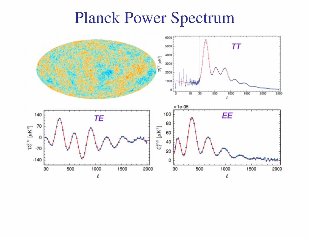
Planck Power Spectrum

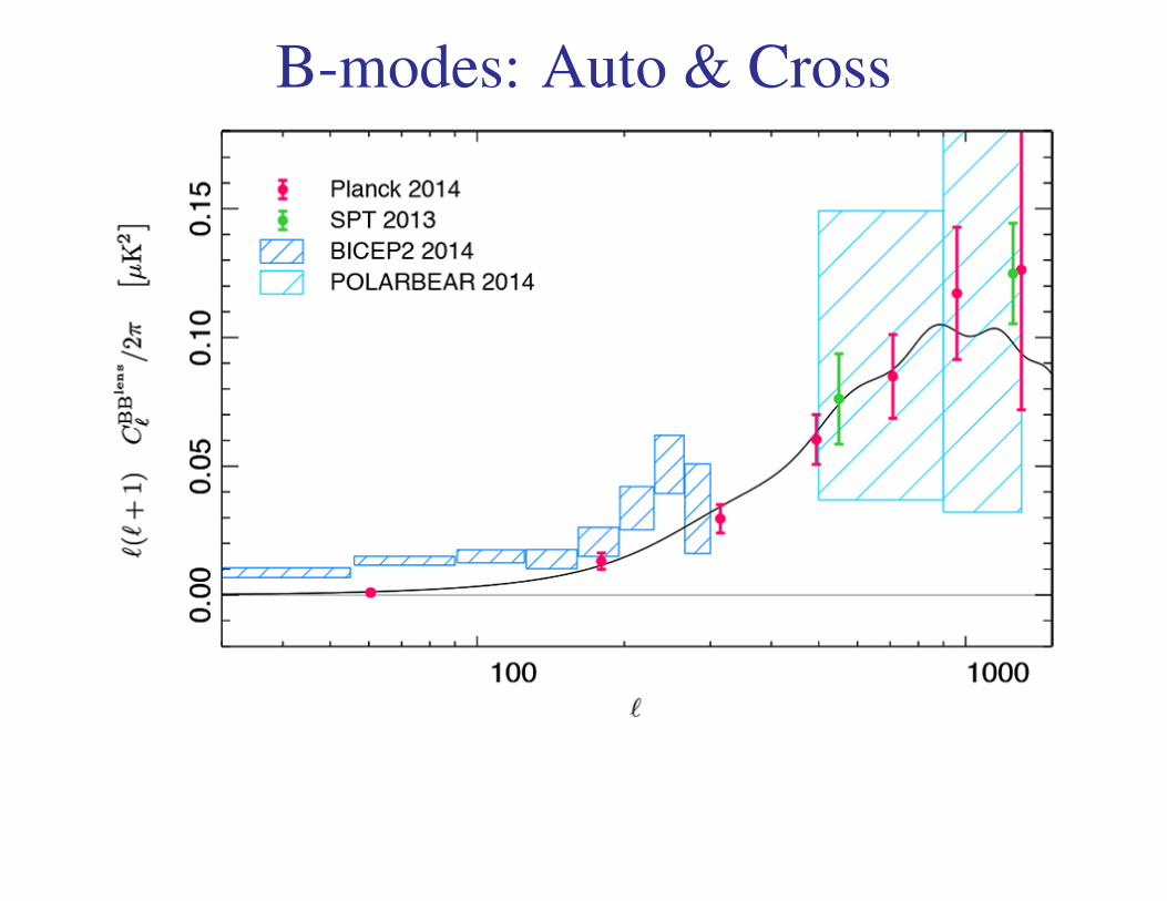
B-modes: Auto & Cross

Scalar Primary Power Spectrum

100

10-1

10-2

101

101 102 103

102

103

reion.τ=0.1

l

Pow

er (

µK2 )

temperature

cross

E-pol.

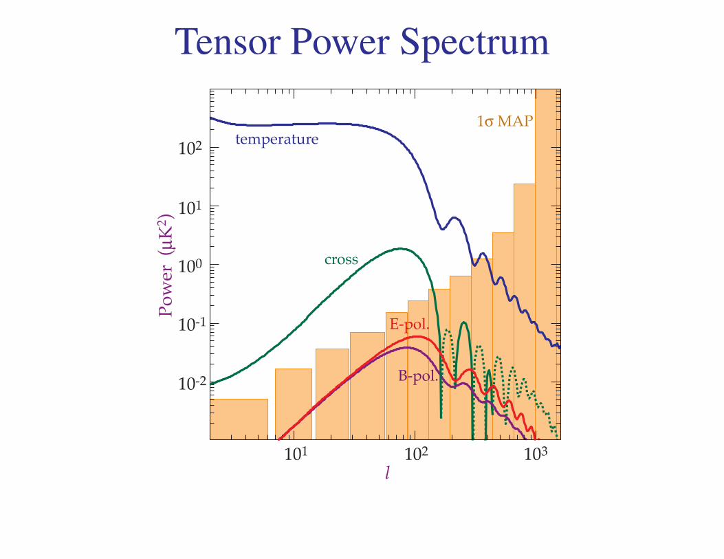
Tensor Power Spectrum

101 102 103

100

10-1

10-2

101

102Po

wer

(µK

2 )

l

temperature

cross

E-pol.

B-pol.

1σ MAP

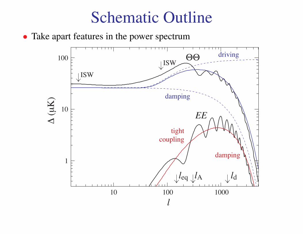
Schematic Outline• Take apart features in the power spectrum

Δ (μK)

10

100

1

10 100 1000

l

leq lA ld

ΘΘ

EE

damping

damping

tightcoupling

drivingISW

ISW

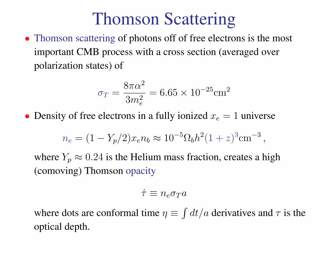
Thomson Scattering• Thomson scattering of photons off of free electrons is the most

important CMB process with a cross section (averaged overpolarization states) of

σT =8πα2

3m2e

= 6.65× 10−25cm2

• Density of free electrons in a fully ionized xe = 1 universe

ne = (1− Yp/2)xenb ≈ 10−5Ωbh2(1 + z)3cm−3 ,

where Yp ≈ 0.24 is the Helium mass fraction, creates a high(comoving) Thomson opacity

τ ≡ neσTa

where dots are conformal time η ≡∫dt/a derivatives and τ is the

optical depth.

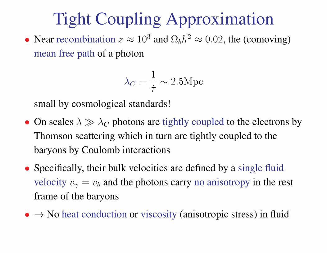
Tight Coupling Approximation• Near recombination z ≈ 103 and Ωbh

2 ≈ 0.02, the (comoving)mean free path of a photon

λC ≡1

τ∼ 2.5Mpc

small by cosmological standards!

• On scales λ λC photons are tightly coupled to the electrons byThomson scattering which in turn are tightly coupled to thebaryons by Coulomb interactions

• Specifically, their bulk velocities are defined by a single fluidvelocity vγ = vb and the photons carry no anisotropy in the restframe of the baryons

• → No heat conduction or viscosity (anisotropic stress) in fluid

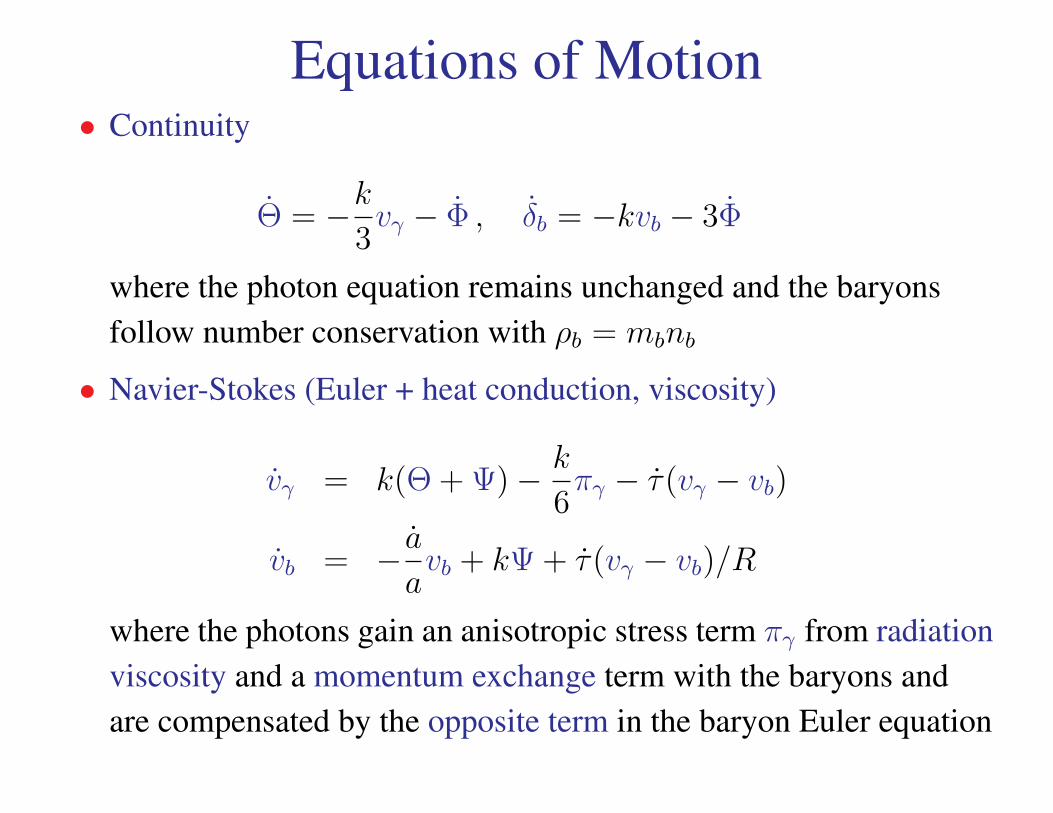
Equations of Motion• Continuity

Θ = −k3vγ − Φ , δb = −kvb − 3Φ

where the photon equation remains unchanged and the baryonsfollow number conservation with ρb = mbnb

• Navier-Stokes (Euler + heat conduction, viscosity)

vγ = k(Θ + Ψ)− k

6πγ − τ(vγ − vb)

vb = − aavb + kΨ + τ(vγ − vb)/R

where the photons gain an anisotropic stress term πγ from radiationviscosity and a momentum exchange term with the baryons andare compensated by the opposite term in the baryon Euler equation

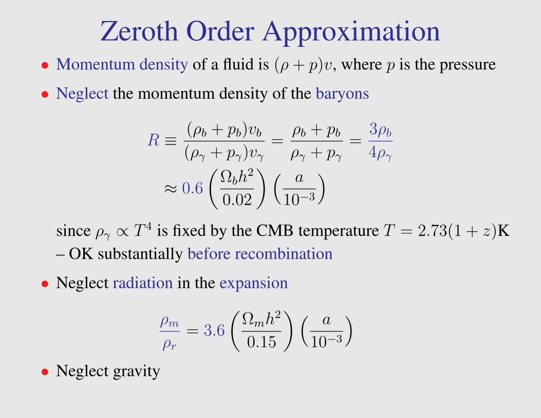
Zeroth Order Approximation• Momentum density of a fluid is (ρ+ p)v, where p is the pressure

• Neglect the momentum density of the baryons

R ≡ (ρb + pb)vb(ργ + pγ)vγ

=ρb + pbργ + pγ

=3ρb4ργ

≈ 0.6

(Ωbh

2

0.02

)( a

10−3

)since ργ ∝ T 4 is fixed by the CMB temperature T = 2.73(1 + z)K– OK substantially before recombination

• Neglect radiation in the expansion

ρmρr

= 3.6

(Ωmh

2

0.15

)( a

10−3

)• Neglect gravity

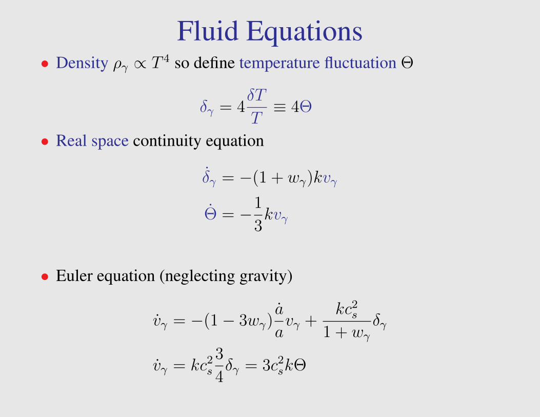
Fluid Equations• Density ργ ∝ T 4 so define temperature fluctuation Θ

δγ = 4δT

T≡ 4Θ

• Real space continuity equation

δγ = −(1 + wγ)kvγ

Θ = −1

3kvγ

• Euler equation (neglecting gravity)

vγ = −(1− 3wγ)a

avγ +

kc2s

1 + wγδγ

vγ = kc2s

3

4δγ = 3c2

skΘ

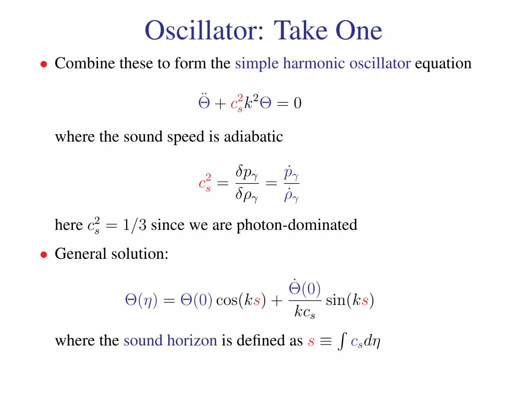
Oscillator: Take One• Combine these to form the simple harmonic oscillator equation

Θ + c2sk

2Θ = 0

where the sound speed is adiabatic

c2s =

δpγδργ

=pγργ

here c2s = 1/3 since we are photon-dominated

• General solution:

Θ(η) = Θ(0) cos(ks) +Θ(0)

kcssin(ks)

where the sound horizon is defined as s ≡∫csdη

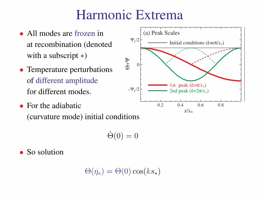
Harmonic Extrema.

Ψi /2

0

–Ψi /2

Θ+Ψ

0.2 0.4 0.6 0.8s/s*

0.2 0.4 0.6 0.8s/s*

1st peak (k=π/s*)

Initial conditions (k<<π/s*)

2nd peak (k=2π/s*)R=1/6

(a) Peak Scales (b) Baryons• All modes are frozen inat recombination (denotedwith a subscript ∗)

• Temperature perturbationsof different amplitudefor different modes.

• For the adiabatic(curvature mode) initial conditions

Θ(0) = 0

• So solution

Θ(η∗) = Θ(0) cos(ks∗)

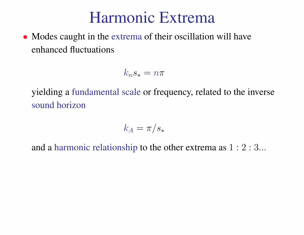
Harmonic Extrema• Modes caught in the extrema of their oscillation will have

enhanced fluctuations

kns∗ = nπ

yielding a fundamental scale or frequency, related to the inversesound horizon

kA = π/s∗

and a harmonic relationship to the other extrema as 1 : 2 : 3...

Peak Location• The fundmental physical scale is translated into a fundamental

angular scale by simple projection according to the angulardiameter distance DA

θA = λA/DA

`A = kADA

• In a flat universe, the distance is simply DA = D ≡ η0 − η∗ ≈ η0,the horizon distance, and kA = π/s∗ =

√3π/η∗ so

θA ≈η∗η0

• In a matter-dominated universe η ∝ a1/2 so θA ≈ 1/30 ≈ 2 or

`A ≈ 200

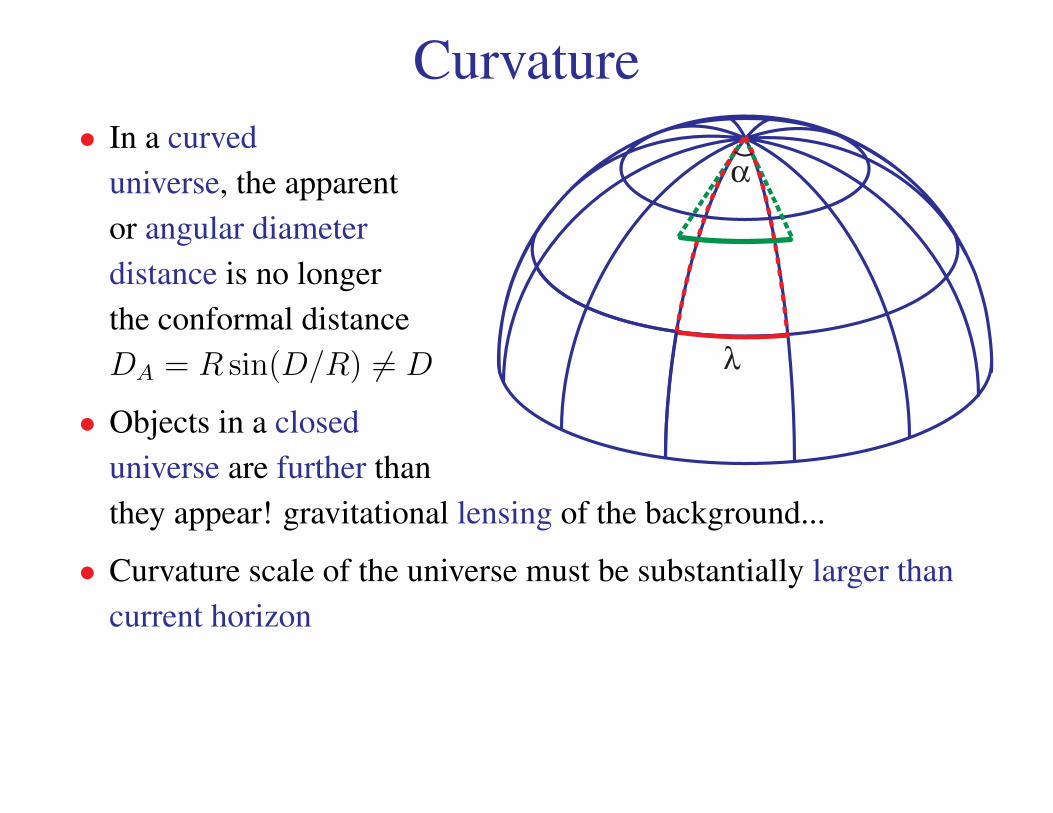
Curvature.

λ

α• In a curved

universe, the apparentor angular diameterdistance is no longerthe conformal distanceDA = R sin(D/R) 6= D

• Objects in a closeduniverse are further thanthey appear! gravitational lensing of the background...

• Curvature scale of the universe must be substantially larger thancurrent horizon

Curvature.

10 100 1000

20

40

60

80

100

l

ΔT

(μK)

Ωtot

0.2 0.4 0.6 0.8 1.0

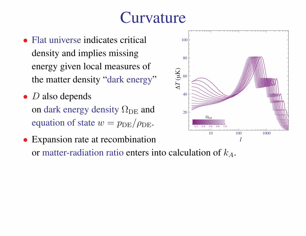
• Flat universe indicates criticaldensity and implies missingenergy given local measures ofthe matter density “dark energy”

• D also dependson dark energy density ΩDE andequation of state w = pDE/ρDE.

• Expansion rate at recombinationor matter-radiation ratio enters into calculation of kA.

Fixed Deceleration Epoch• CMB determination of matter density controls all determinations

in the deceleration (matter dominated) epoch

• Planck: Ωmh2 = 0.1426± 0.0025→ 1.7%

• Distance to recombination D∗ determined to 141.7% ≈ 0.43%

(ΛCDM result 0.46%; ∆h/h ≈ −∆Ωmh2/Ωmh

2)[more general: −0.11∆w − 0.48∆ lnh− 0.15∆ ln Ωm − 1.4∆ ln Ωtot = 0 ]

• Expansion rate during any redshift in the deceleration epochdetermined to 1

21.7%

• Distance to any redshift in the deceleration epoch determined as

D(z) = D∗ −∫ z∗

z

dz

H(z)

• Volumes determined by a combination dV = D2AdΩdz/H(z)

• Structure also determined by growth of fluctuations from z∗

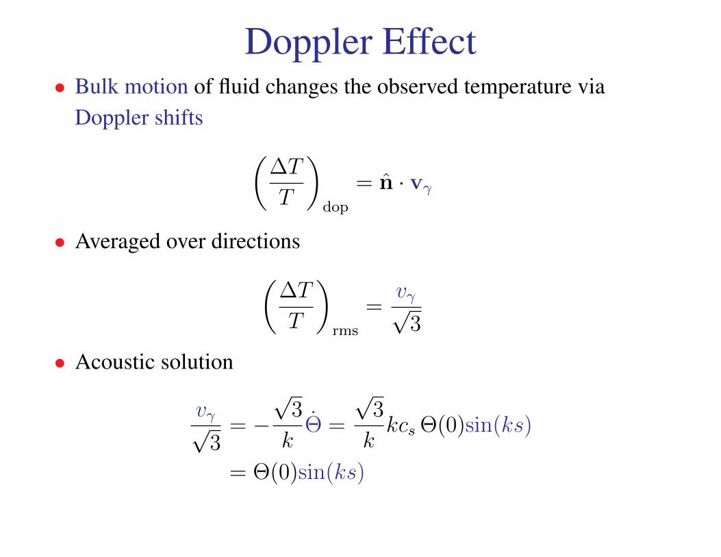
Doppler Effect• Bulk motion of fluid changes the observed temperature via

Doppler shifts (∆T

T

)dop

= n · vγ

• Averaged over directions(∆T

T

)rms

=vγ√

3

• Acoustic solution

vγ√3

= −√

3

kΘ =

√3

kkcs Θ(0)sin(ks)

= Θ(0)sin(ks)

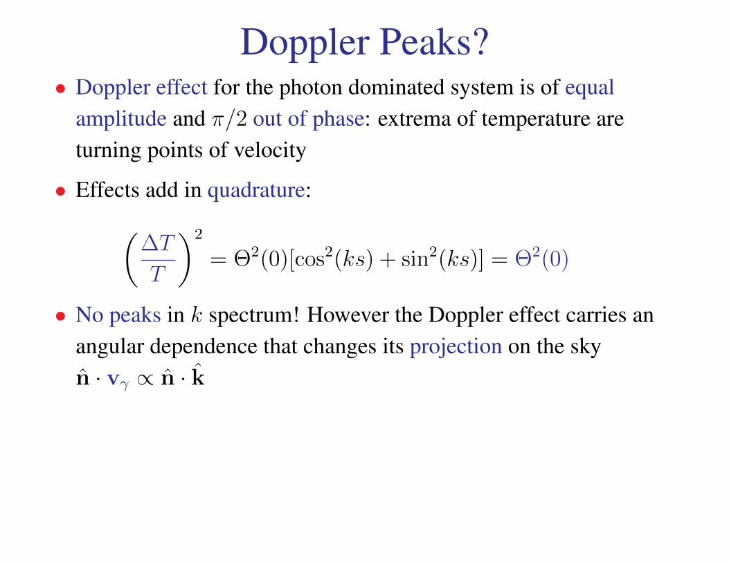
Doppler Peaks?• Doppler effect for the photon dominated system is of equal

amplitude and π/2 out of phase: extrema of temperature areturning points of velocity

• Effects add in quadrature:(∆T

T

)2

= Θ2(0)[cos2(ks) + sin2(ks)] = Θ2(0)

• No peaks in k spectrum! However the Doppler effect carries anangular dependence that changes its projection on the skyn · vγ ∝ n · k

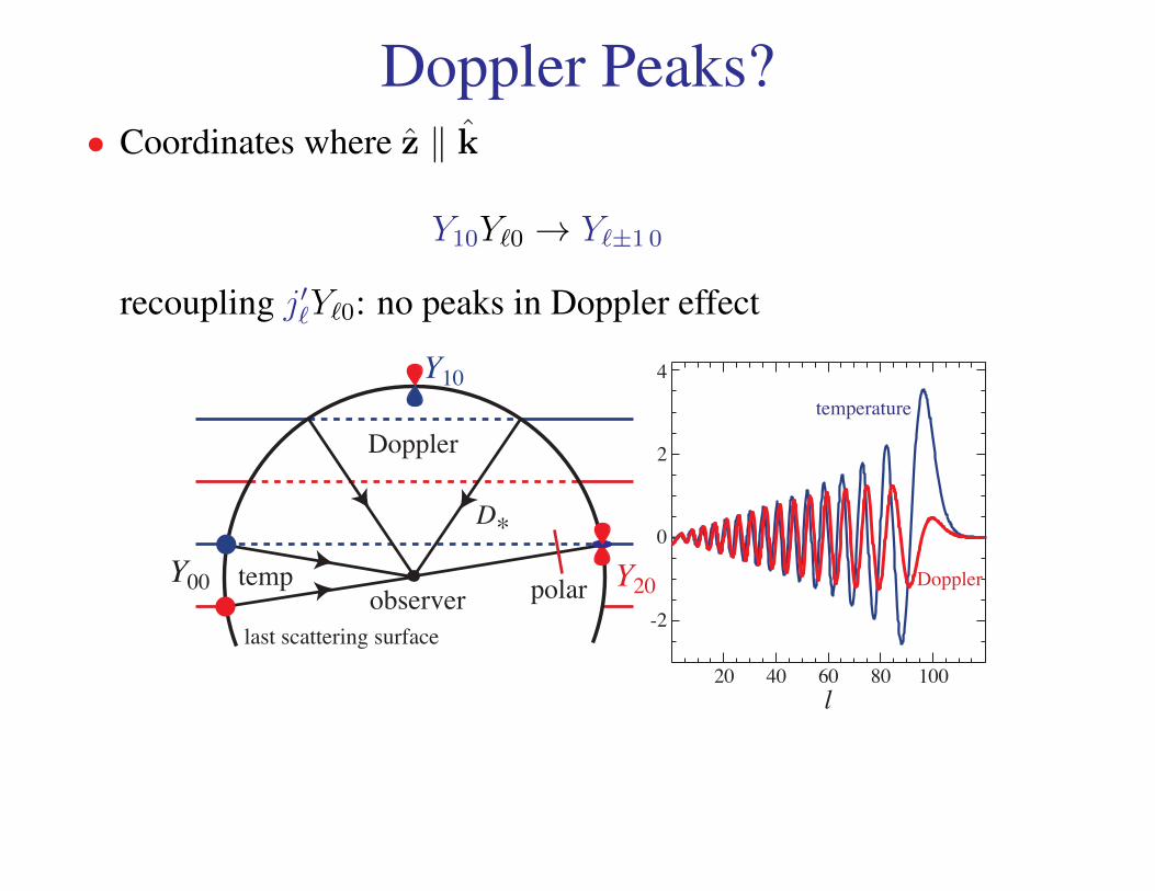
Doppler Peaks?• Coordinates where z ‖ k

Y10Y`0 → Y`±1 0

recoupling j′`Y`0: no peaks in Doppler effect

l20 40

4

2

0

-2

60 80 100

observerY20Y00

Y10

temp

Doppler

polar

D*

last scattering surface

temperature

Doppler

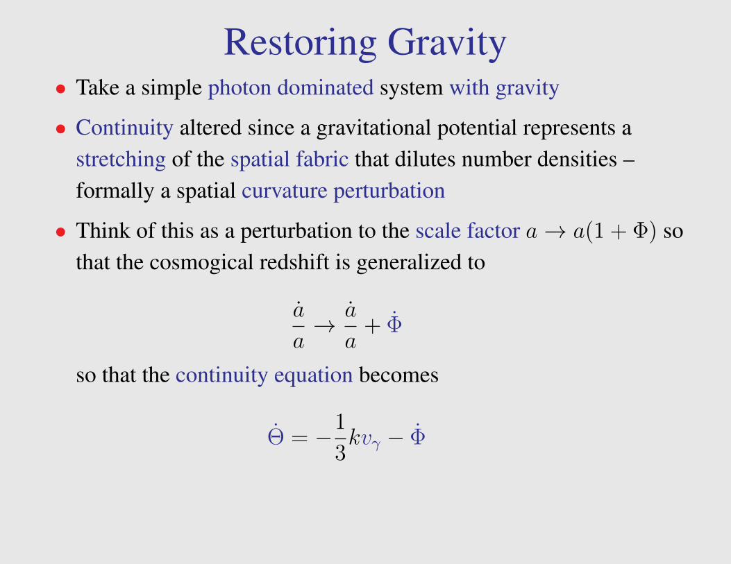
Restoring Gravity• Take a simple photon dominated system with gravity

• Continuity altered since a gravitational potential represents astretching of the spatial fabric that dilutes number densities –formally a spatial curvature perturbation

• Think of this as a perturbation to the scale factor a→ a(1 + Φ) sothat the cosmogical redshift is generalized to

a

a→ a

a+ Φ

so that the continuity equation becomes

Θ = −1

3kvγ − Φ

Restoring Gravity• Gravitational force in momentum conservation F = −m∇Ψ

generalized to momentum density modifies the Euler equation to

vγ = k(Θ + Ψ)

• General relativity says that Φ and Ψ are the relativistic analoguesof the Newtonian potential and that Φ ≈ −Ψ.

• In our matter-dominated approximation, Φ represents matterdensity fluctuations through the cosmological Poisson equation

k2Φ = 4πGa2ρm∆m

where the difference comes from the use of comoving coordinatesfor k (a2 factor), the removal of the background density into thebackground expansion (ρ∆m) and finally a coordinate subtlety thatenters into the definition of ∆m

Constant Potentials• In the matter dominated epoch potentials are constant because

infall generates velocities as vm ∼ kηΨ

• Velocity divergence generates density perturbations as∆m ∼ −kηvm ∼ −(kη)2Ψ

• And density perturbations generate potential fluctuations

Φ =4πGa2ρ∆

k2≈ 3

2

H2a2

k2∆ ∼ ∆

(kη)2∼ −Ψ

keeping them constant. Note that because of the expansion, densityperturbations must grow to keep potentials constant.

Constant Potentials• More generally, if stress perturbations are negligible compared

with density perturbations ( δp δρ ) then potential will remainroughly constant

• More specifically a variant called the Bardeen or comovingcurvature is strictly constant

R = const ≈ 5 + 3w

3 + 3wΦ

where the approximation holds when w ≈const.

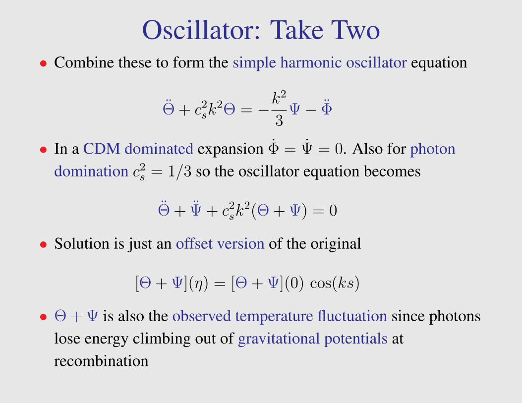
Oscillator: Take Two• Combine these to form the simple harmonic oscillator equation

Θ + c2sk

2Θ = −k2

3Ψ− Φ

• In a CDM dominated expansion Φ = Ψ = 0. Also for photondomination c2

s = 1/3 so the oscillator equation becomes

Θ + Ψ + c2sk

2(Θ + Ψ) = 0

• Solution is just an offset version of the original

[Θ + Ψ](η) = [Θ + Ψ](0) cos(ks)

• Θ + Ψ is also the observed temperature fluctuation since photonslose energy climbing out of gravitational potentials atrecombination

Effective Temperature• Photons climb out of potential wells at last scattering

• Lose energy to gravitational redshifts

• Observed or effective temperature

Θ + Ψ

• Effective temperature oscillates around zero with amplitude givenby the initial conditions

• Note: initial conditions are set when the perturbation is outside ofhorizon, need inflation or other modification to matter-radiationFRW universe.

• GR says that initial temperature is given by initial potential

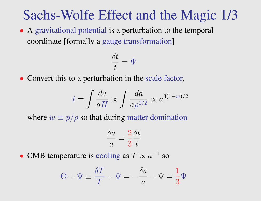
Sachs-Wolfe Effect and the Magic 1/3• A gravitational potential is a perturbation to the temporal

coordinate [formally a gauge transformation]

δt

t= Ψ

• Convert this to a perturbation in the scale factor,

t =

∫da

aH∝∫

da

aρ1/2∝ a3(1+w)/2

where w ≡ p/ρ so that during matter domination

δa

a=

2

3

δt

t

• CMB temperature is cooling as T ∝ a−1 so

Θ + Ψ ≡ δT

T+ Ψ = −δa

a+ Ψ =

1

3Ψ

Sachs-Wolfe Normalization• Use measurements of ∆T/T ≈ 10−5 in the Sachs-Wolfe effect to

infer ∆2R

• Recall in matter domination Ψ = −3R/5

`(`+ 1)C`2π

≈ ∆2T ≈

1

25∆2R

• So that the amplitude of initial curvature fluctuations is∆R ≈ 5× 10−5

• Modern usage: WMAP’s measurement of 1st peak plus knownradiation transfer function is used to convert ∆T/T to ∆R.

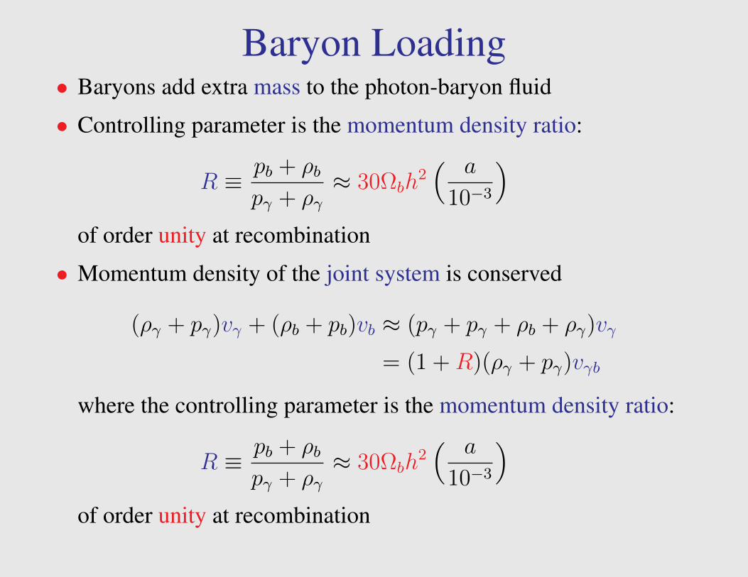
Baryon Loading• Baryons add extra mass to the photon-baryon fluid

• Controlling parameter is the momentum density ratio:

R ≡ pb + ρbpγ + ργ

≈ 30Ωbh2( a

10−3

)of order unity at recombination

• Momentum density of the joint system is conserved

(ργ + pγ)vγ + (ρb + pb)vb ≈ (pγ + pγ + ρb + ργ)vγ

= (1 +R)(ργ + pγ)vγb

where the controlling parameter is the momentum density ratio:

R ≡ pb + ρbpγ + ργ

≈ 30Ωbh2( a

10−3

)of order unity at recombination

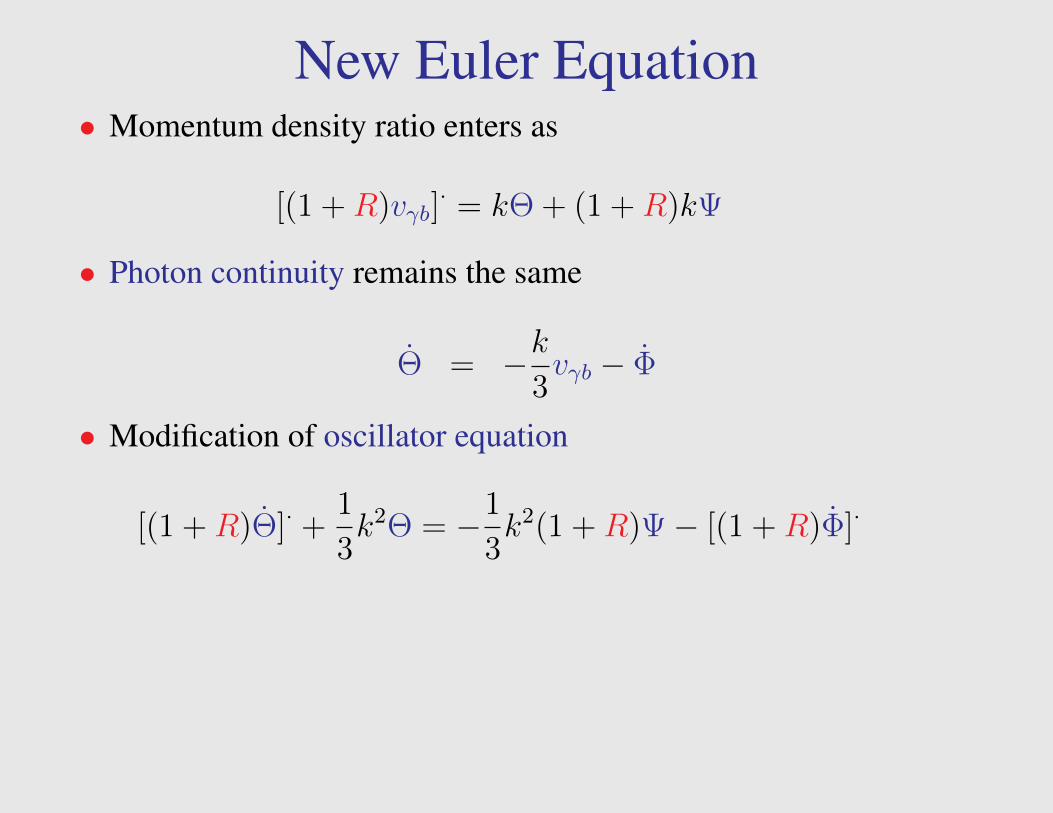
New Euler Equation• Momentum density ratio enters as

[(1 +R)vγb]· = kΘ + (1 +R)kΨ

• Photon continuity remains the same

Θ = −k3vγb − Φ

• Modification of oscillator equation

[(1 +R)Θ]· +1

3k2Θ = −1

3k2(1 +R)Ψ− [(1 +R)Φ]·

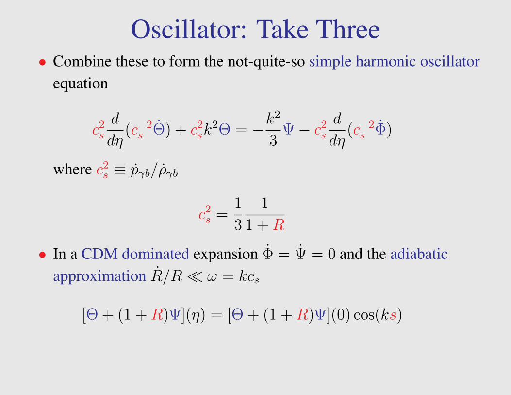
Oscillator: Take Three• Combine these to form the not-quite-so simple harmonic oscillator

equation

c2s

d

dη(c−2s Θ) + c2

sk2Θ = −k

2

3Ψ− c2

s

d

dη(c−2s Φ)

where c2s ≡ pγb/ργb

c2s =

1

3

1

1 +R

• In a CDM dominated expansion Φ = Ψ = 0 and the adiabaticapproximation R/R ω = kcs

[Θ + (1 +R)Ψ](η) = [Θ + (1 +R)Ψ](0) cos(ks)

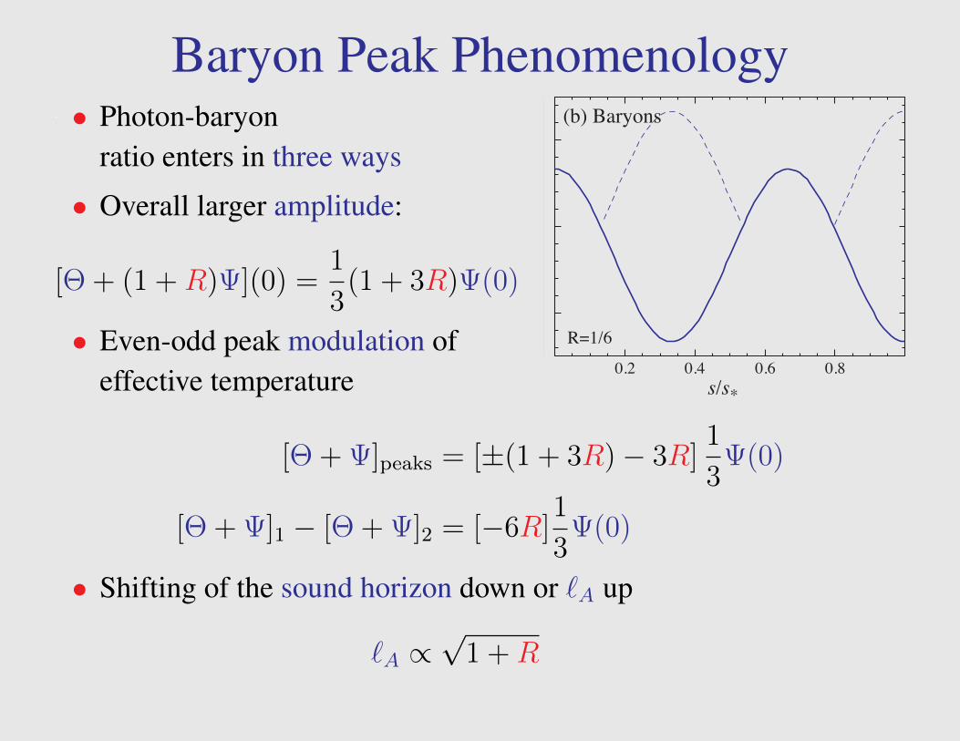
Baryon Peak Phenomenology.

Ψi /2

0

–Ψi /2

Θ+Ψ

0.2 0.4 0.6 0.8s/s*

0.2 0.4 0.6 0.8s/s*

1st peak (k=π/s*)

Initial conditions (k<<π/s*)

2nd peak (k=2π/s*)R=1/6

(a) Peak Scales (b) Baryons• Photon-baryonratio enters in three ways

• Overall larger amplitude:

[Θ + (1 +R)Ψ](0) =1

3(1 + 3R)Ψ(0)

• Even-odd peak modulation ofeffective temperature

[Θ + Ψ]peaks = [±(1 + 3R)− 3R]1

3Ψ(0)

[Θ + Ψ]1 − [Θ + Ψ]2 = [−6R]1

3Ψ(0)

• Shifting of the sound horizon down or `A up

`A ∝√

1 +R

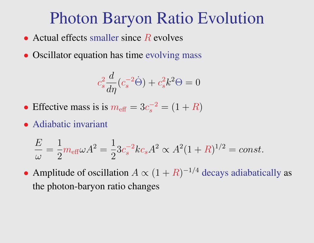
Photon Baryon Ratio Evolution• Actual effects smaller since R evolves

• Oscillator equation has time evolving mass

c2s

d

dη(c−2s Θ) + c2

sk2Θ = 0

• Effective mass is is meff = 3c−2s = (1 +R)

• Adiabatic invariant

E

ω=

1

2meffωA

2 =1

23c−2s kcsA

2 ∝ A2(1 +R)1/2 = const.

• Amplitude of oscillation A ∝ (1 +R)−1/4 decays adiabatically asthe photon-baryon ratio changes

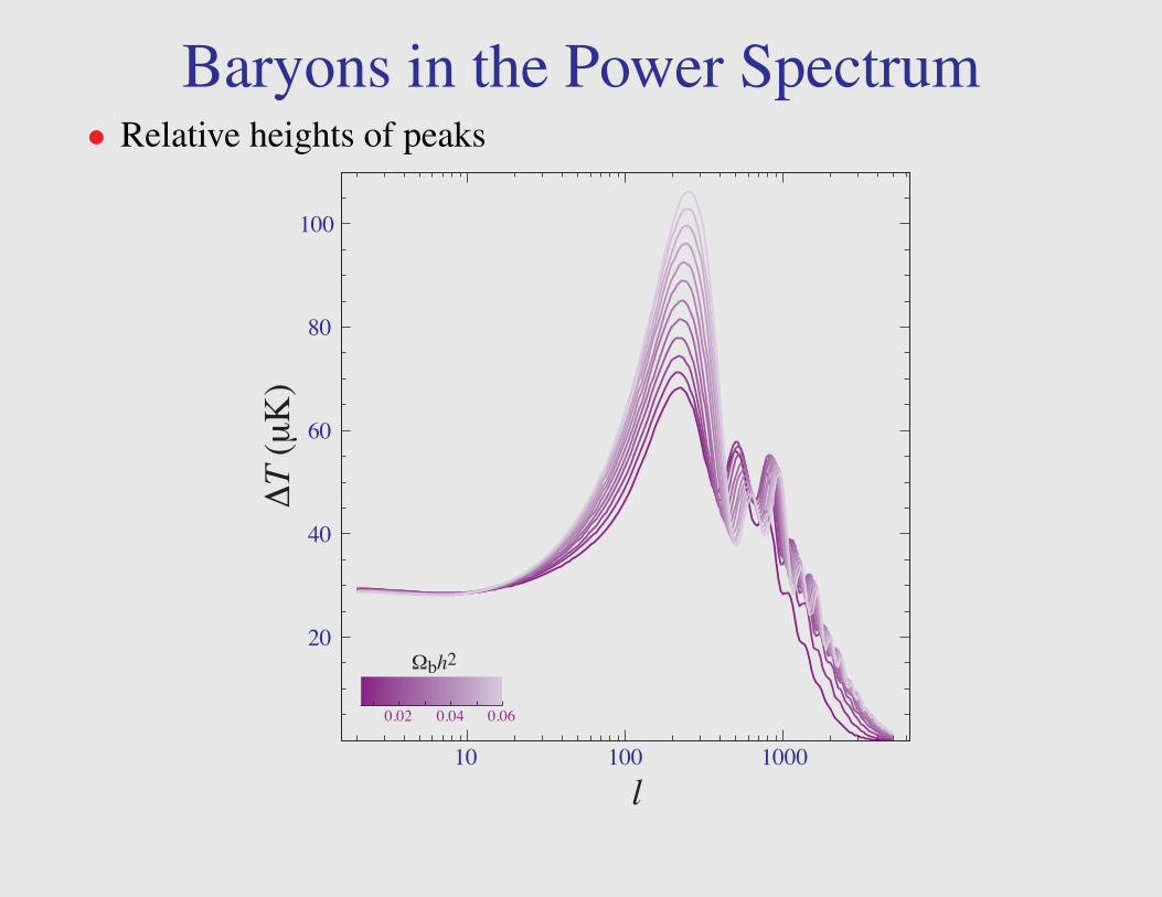
Baryons in the Power Spectrum• Relative heights of peaks

Ωbh2

10

0.02 0.04 0.06

100 1000

20

40

60

80

100

l

ΔT

(μK)

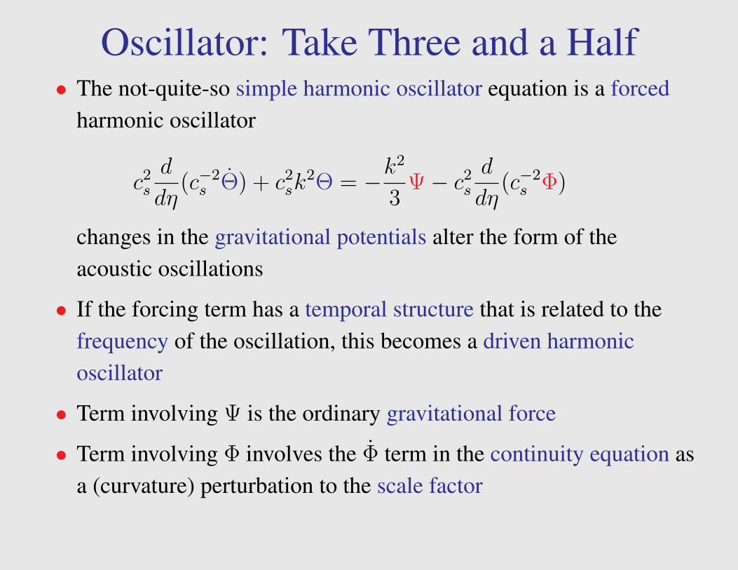
Oscillator: Take Three and a Half• The not-quite-so simple harmonic oscillator equation is a forced

harmonic oscillator

c2s

d

dη(c−2s Θ) + c2

sk2Θ = −k

2

3Ψ− c2

s

d

dη(c−2s Φ)

changes in the gravitational potentials alter the form of theacoustic oscillations

• If the forcing term has a temporal structure that is related to thefrequency of the oscillation, this becomes a driven harmonicoscillator

• Term involving Ψ is the ordinary gravitational force

• Term involving Φ involves the Φ term in the continuity equation asa (curvature) perturbation to the scale factor

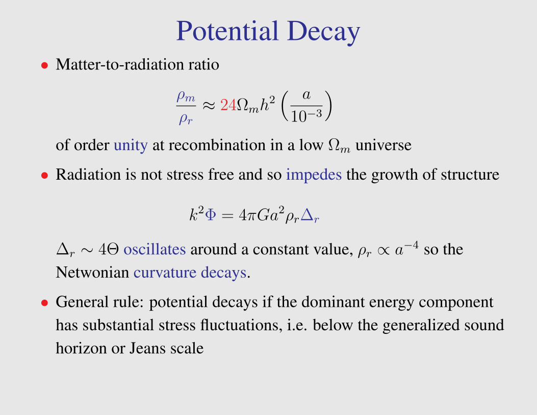
Potential Decay• Matter-to-radiation ratio

ρmρr≈ 24Ωmh

2( a

10−3

)of order unity at recombination in a low Ωm universe

• Radiation is not stress free and so impedes the growth of structure

k2Φ = 4πGa2ρr∆r

∆r ∼ 4Θ oscillates around a constant value, ρr ∝ a−4 so theNetwonian curvature decays.

• General rule: potential decays if the dominant energy componenthas substantial stress fluctuations, i.e. below the generalized soundhorizon or Jeans scale

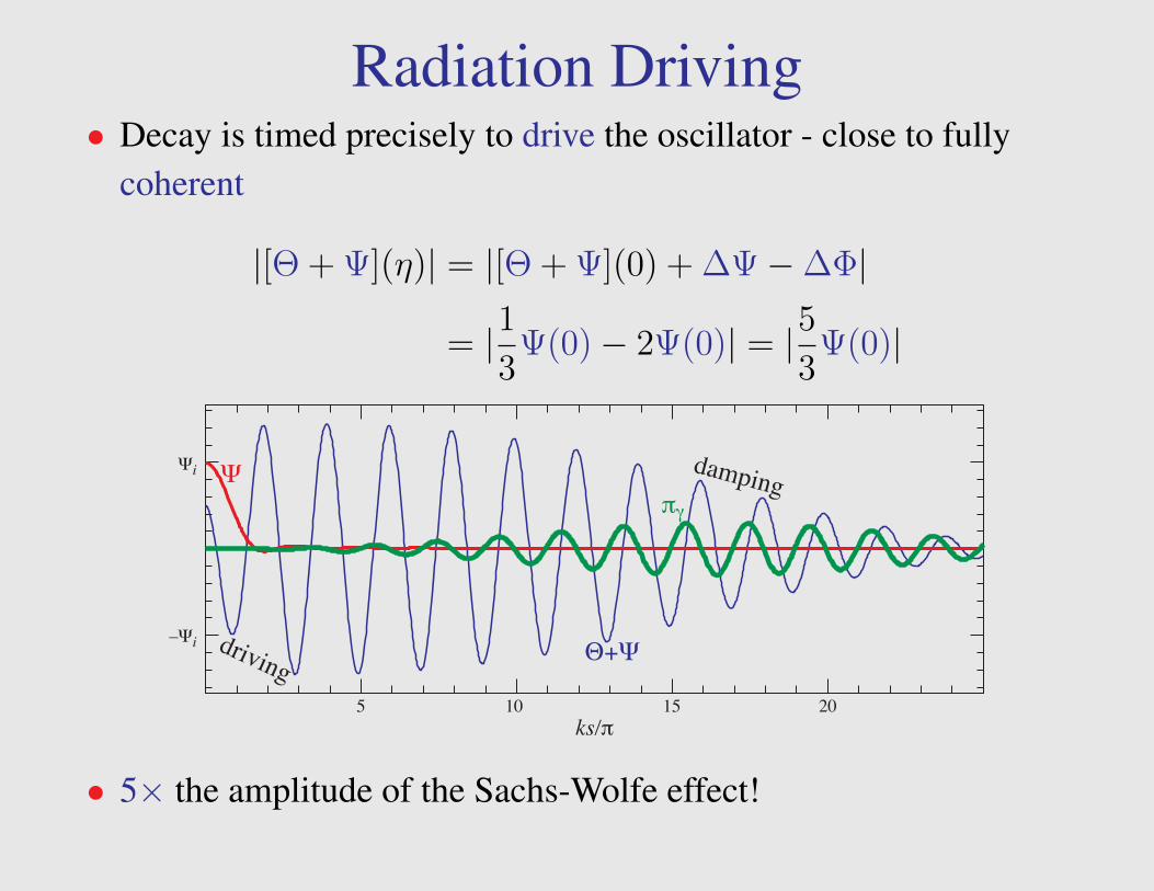
Radiation Driving• Decay is timed precisely to drive the oscillator - close to fully

coherent

|[Θ + Ψ](η)| = |[Θ + Ψ](0) + ∆Ψ−∆Φ|

= |13

Ψ(0)− 2Ψ(0)| = |53

Ψ(0)|

105 15 20

Ψi

–Ψi

Ψ

Θ+Ψ

πγ

ks/π

damping

driving

• 5× the amplitude of the Sachs-Wolfe effect!

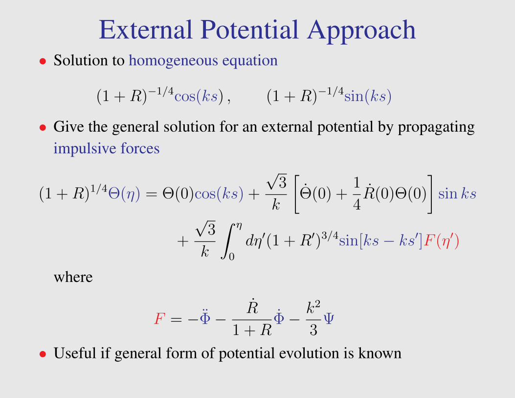
External Potential Approach• Solution to homogeneous equation

(1 +R)−1/4cos(ks) , (1 +R)−1/4sin(ks)

• Give the general solution for an external potential by propagatingimpulsive forces

(1 +R)1/4Θ(η) = Θ(0)cos(ks) +

√3

k

[Θ(0) +

1

4R(0)Θ(0)

]sin ks

+

√3

k

∫ η

0

dη′(1 +R′)3/4sin[ks− ks′]F (η′)

where

F = −Φ− R

1 +RΦ− k2

3Ψ

• Useful if general form of potential evolution is known

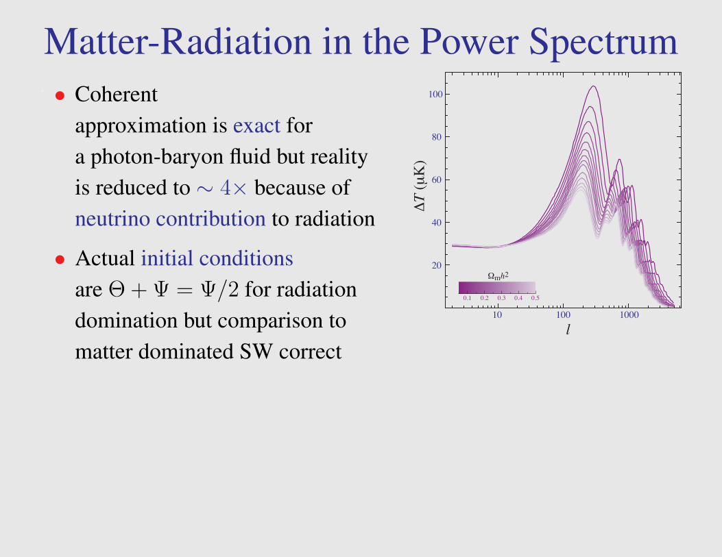
Matter-Radiation in the Power Spectrum.

10 100 1000

20

40

60

80

100

l

ΔT

(μK)

Ωmh2

0.1 0.2 0.3 0.4 0.5

• Coherentapproximation is exact fora photon-baryon fluid but realityis reduced to ∼ 4× because ofneutrino contribution to radiation

• Actual initial conditionsare Θ + Ψ = Ψ/2 for radiationdomination but comparison tomatter dominated SW correct

Damping• Tight coupling equations assume a perfect fluid: no viscosity, no

heat conduction

• Fluid imperfections are related to the mean free path of thephotons in the baryons

λC = τ−1 where τ = neσTa

is the conformal opacity to Thomson scattering

• Dissipation related to diffusion length: random walk approx

λD =√NλC =

√η/λC λC =

√ηλC

the geometric mean between the horizon and mean free path

• λD/η∗ ∼ few %, so expect peaks > 3 to be affected by dissipation

• √η enters here and η in the acoustic scale→ expansion rate andextra relativistic species

Equations of Motion• Continuity

Θ = −k3vγ − Φ , δb = −kvb − 3Φ

where the photon equation remains unchanged and the baryonsfollow number conservation with ρb = mbnb

• Navier-Stokes (Euler + heat conduction, viscosity)

vγ = k(Θ + Ψ)− k

6πγ − τ(vγ − vb)

vb = − aavb + kΨ + τ(vγ − vb)/R

where the photons gain an anisotropic stress term πγ from radiationviscosity and a momentum exchange term with the baryons andare compensated by the opposite term in the baryon Euler equation

Viscosity• Viscosity is generated from radiation streaming from hot to cold

regions

• Expect

πγ ∼ vγk

τ

generated by streaming, suppressed by scattering in a wavelengthof the fluctuation. Radiative transfer says

πγ ≈ 2Avvγk

τ

where Av = 16/15

vγ = k(Θ + Ψ)− k

3Avk

τvγ

Oscillator: Penultimate Take• Adiabatic approximation ( ω a/a)

Θ ≈ −k3vγ

• Oscillator equation contains a Θ damping term

c2s

d

dη(c−2s Θ) +

k2c2s

τAvΘ + k2c2

sΘ = −k2

3Ψ− c2

s

d

dη(c−2s Φ)

• Heat conduction term similar in that it is proportional to vγ and issuppressed by scattering k/τ . Expansion of Euler equations toleading order in kτ gives

Ah =R2

1 +R

since the effects are only significant if the baryons are dynamicallyimportant

Oscillator: Final Take• Final oscillator equation

c2s

d

dη(c−2s Θ) +

k2c2s

τ[Av + Ah]Θ + k2c2

sΘ = −k2

3Ψ− c2

s

d

dη(c−2s Φ)

• Solve in the adiabatic approximation

Θ ∝ exp(i

∫ωdη)

−ω2 +k2c2

s

τ(Av + Ah)iω + k2c2

s = 0

Dispersion Relation• Solve

ω2 = k2c2s

[1 + i

ω

τ(Av + Ah)

]ω = ±kcs

[1 +

i

2

ω

τ(Av + Ah)

]= ±kcs

[1± i

2

kcsτ

(Av + Ah)

]• Exponentiate

exp(i

∫ωdη) = e±iks exp[−k2

∫dη

1

2

c2s

τ(Av + Ah)]

= e±iks exp[−(k/kD)2]

• Damping is exponential under the scale kD

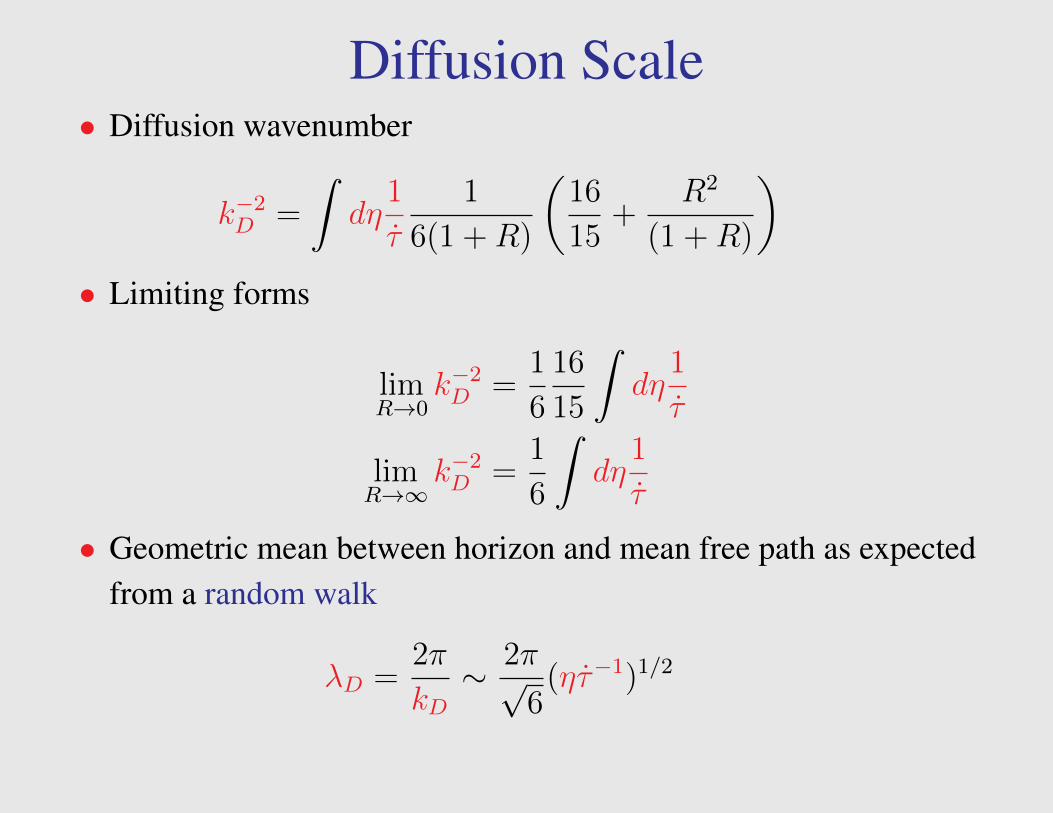
Diffusion Scale• Diffusion wavenumber

k−2D =

∫dη

1

τ

1

6(1 +R)

(16

15+

R2

(1 +R)

)• Limiting forms

limR→0

k−2D =

1

6

16

15

∫dη

1

τ

limR→∞

k−2D =

1

6

∫dη

1

τ

• Geometric mean between horizon and mean free path as expectedfrom a random walk

λD =2π

kD∼ 2π√

6(ητ−1)1/2

Thomson Scattering• Polarization state of radiation in direction n described by the

intensity matrix⟨Ei(n)E∗j (n)

⟩, where E is the electric field vector

and the brackets denote time averaging.

• Differential cross section

dσ

dΩ=

3

8π|E′ · E|2σT ,

where σT = 8πα2/3me is the Thomson cross section, E′ and E

denote the incoming and outgoing directions of the electric field orpolarization vector.

• Summed over angle and incoming polarization∑i=1,2

∫dn′

dσ

dΩ= σT

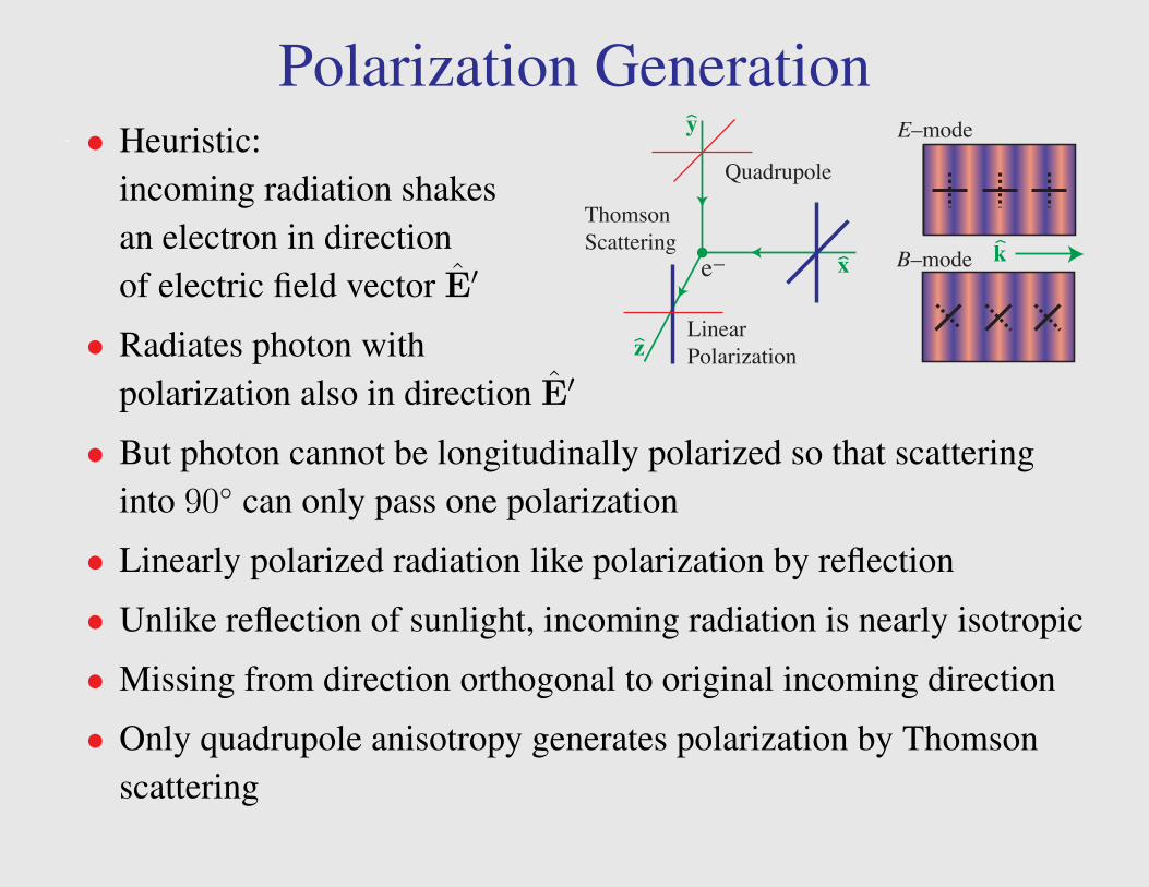
Polarization Generation. E–mode

B–modee–

LinearPolarization

ThomsonScattering

Quadrupole

x k

y

z

• Heuristic:incoming radiation shakesan electron in directionof electric field vector E′

• Radiates photon withpolarization also in direction E′

• But photon cannot be longitudinally polarized so that scatteringinto 90 can only pass one polarization

• Linearly polarized radiation like polarization by reflection

• Unlike reflection of sunlight, incoming radiation is nearly isotropic

• Missing from direction orthogonal to original incoming direction

• Only quadrupole anisotropy generates polarization by Thomsonscattering

Acoustic Polarization• Break down of tight-coupling leads to quadrupole anisotropy of

πγ ≈k

τvγ

• Scaling kD = (τ /η∗)1/2 → τ = k2

Dη∗

• Know: kDs∗ ≈ kDη∗ ≈ 10

• So:

πγ ≈k

kD

1

10vγ

∆P ≈`

`D

1

10∆T

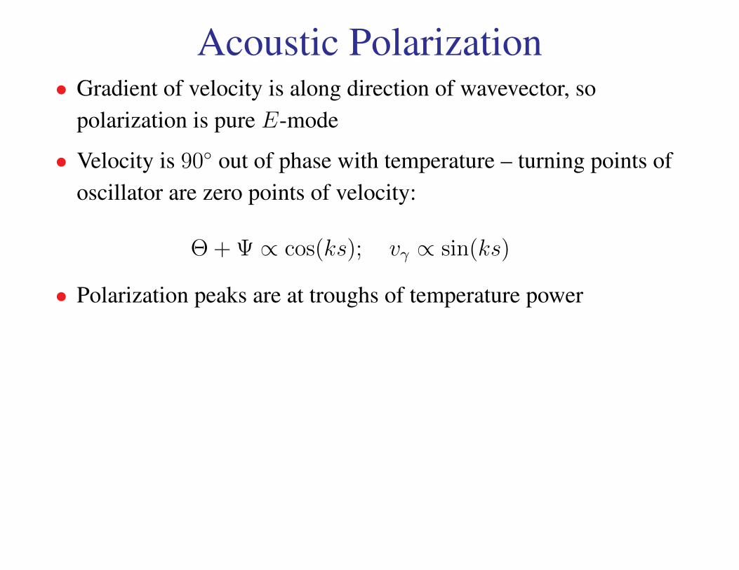
Acoustic Polarization• Gradient of velocity is along direction of wavevector, so

polarization is pure E-mode

• Velocity is 90 out of phase with temperature – turning points ofoscillator are zero points of velocity:

Θ + Ψ ∝ cos(ks); vγ ∝ sin(ks)

• Polarization peaks are at troughs of temperature power

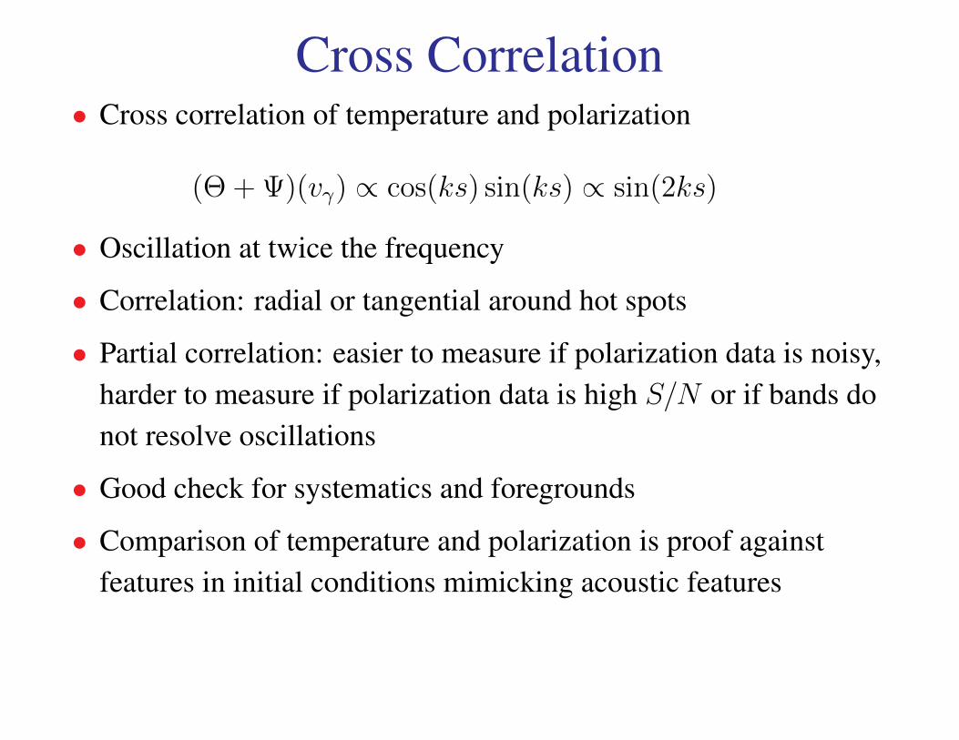
Cross Correlation• Cross correlation of temperature and polarization

(Θ + Ψ)(vγ) ∝ cos(ks) sin(ks) ∝ sin(2ks)

• Oscillation at twice the frequency

• Correlation: radial or tangential around hot spots

• Partial correlation: easier to measure if polarization data is noisy,harder to measure if polarization data is high S/N or if bands donot resolve oscillations

• Good check for systematics and foregrounds

• Comparison of temperature and polarization is proof againstfeatures in initial conditions mimicking acoustic features

Reionization. • Reionization causes

rescattering of radiation

• Suppresses temperature anisotopyas e−τ and changes interpretationof amplitude to Ase−2τ

• Electron sees temperatureanisotropy on its recombinationsurface

• For wavelengths that are comparable to the horizon at reionization,a quadrupole moment

• Rescatters to a linear polarization that is correlated with theSachs-Wolfe temperature anisotropy

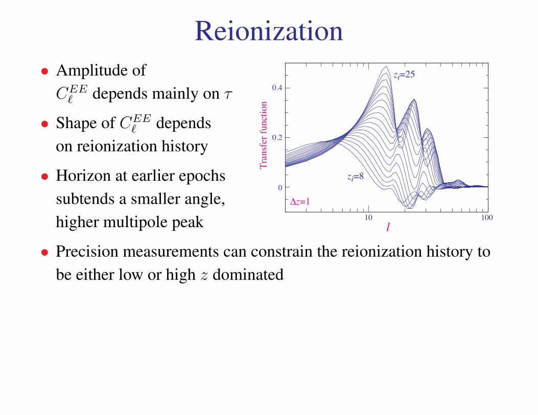
Reionization.

zi=25

zi=8

∆z=1

l

Tran

sfer

func

tion

10 100

0

0.2

0.4

• Amplitude ofCEE` depends mainly on τ

• Shape of CEE` depends

on reionization history

• Horizon at earlier epochssubtends a smaller angle,higher multipole peak

• Precision measurements can constrain the reionization history tobe either low or high z dominated

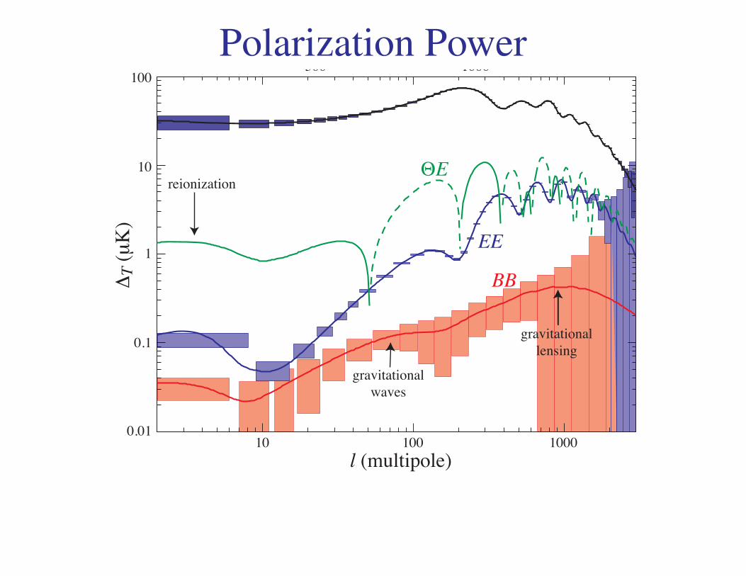
Polarization Power

P OVRO

IAIABIA

SPSSPS

B MBAAAMB MMBB

RI

ViperV

BBABABABBBBBBBAABABB

ING

WDWD

I

SSSSSSSS

CCATC

TTTOTT OOOOOOOOOOOOCOOCOOCOCCOCOOOO OOOOOOOaskSaa

CBI

500 1000

20

40

60

80

ΔT (μK)

Booom98o

DASI00D

Maxxima1x

100

10

10 100 1000

1

0.1

0.01

l (multipole)

ΔT (μK)

reionization

gravitationalwaves

gravitationallensing

ΘE

EE

BB

10 20 30 40

10

20

30

40

50

COBEEE

Ten

FIRSFIRSFIRS

SP

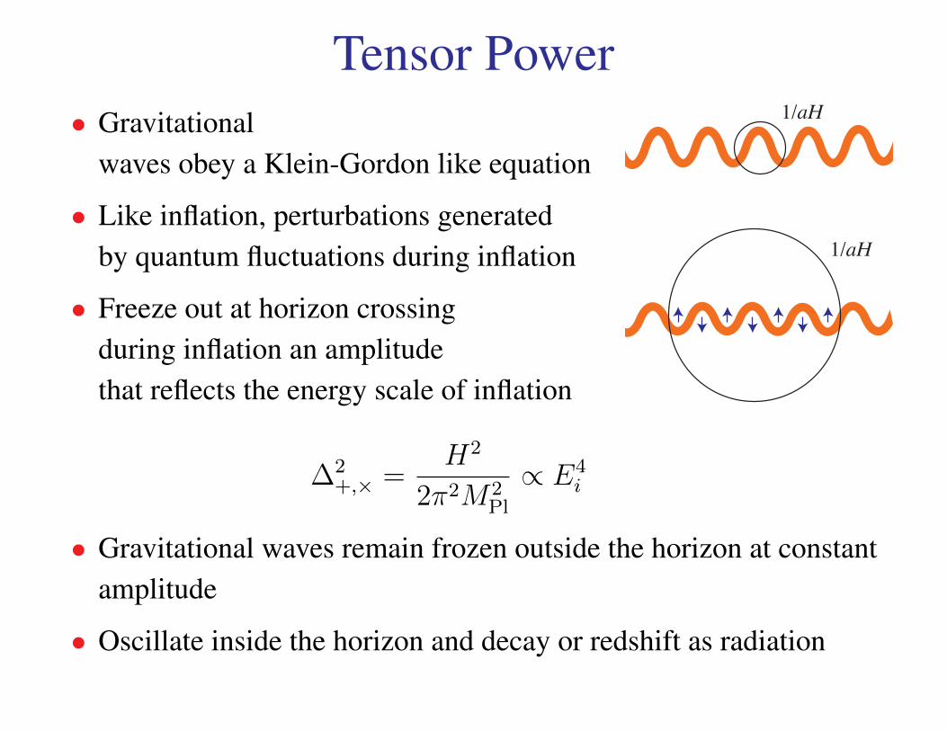
Tensor Power.

1/aH

1/aH• Gravitationalwaves obey a Klein-Gordon like equation

• Like inflation, perturbations generatedby quantum fluctuations during inflation

• Freeze out at horizon crossingduring inflation an amplitudethat reflects the energy scale of inflation

∆2+,× =

H2

2π2M2Pl

∝ E4i

• Gravitational waves remain frozen outside the horizon at constantamplitude

• Oscillate inside the horizon and decay or redshift as radiation

Tensor Quadrupoles.

crest

trough

trough

m=2

Tensors(Gravity Waves)

• Changing transverse-tracelessdistortion of space creates aquadrupole CMB anisotropymuch like the distortionof test ring of particles

• As the tensor mode enters thehorizon it imprints a quadrupoletemperature distortion: H±2

T is source to S±22

• Modes that cross before recombination: effect erased byrescattering e−τ in the integral solution

• Modes that cross after recombination: integrate contributionsalong the line of sight - tensor ISW effect

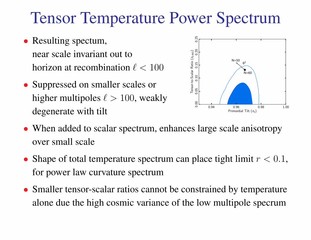
Tensor Temperature Power Spectrum.

0.94 0.96 0.98 1.00Primordial Tilt (ns)

0.00

0.05

0.10

0.15

0.20

0.25

Tensor-to-ScalarRatio

(r0.002)

N=60

N=50φ2

• Resulting spectum,near scale invariant out tohorizon at recombination ` < 100

• Suppressed on smaller scales orhigher multipoles ` > 100, weaklydegenerate with tilt

• When added to scalar spectrum, enhances large scale anisotropyover small scale

• Shape of total temperature spectrum can place tight limit r < 0.1,for power law curvature spectrum

• Smaller tensor-scalar ratios cannot be constrained by temperaturealone due the high cosmic variance of the low multipole specrum

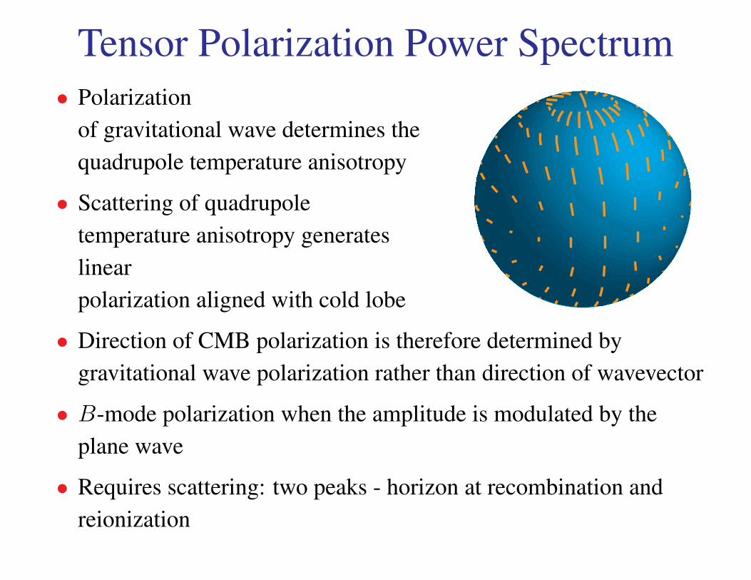
Tensor Polarization Power Spectrum. • Polarization

of gravitational wave determines thequadrupole temperature anisotropy

• Scattering of quadrupoletemperature anisotropy generateslinearpolarization aligned with cold lobe

• Direction of CMB polarization is therefore determined bygravitational wave polarization rather than direction of wavevector

• B-mode polarization when the amplitude is modulated by theplane wave

• Requires scattering: two peaks - horizon at recombination andreionization

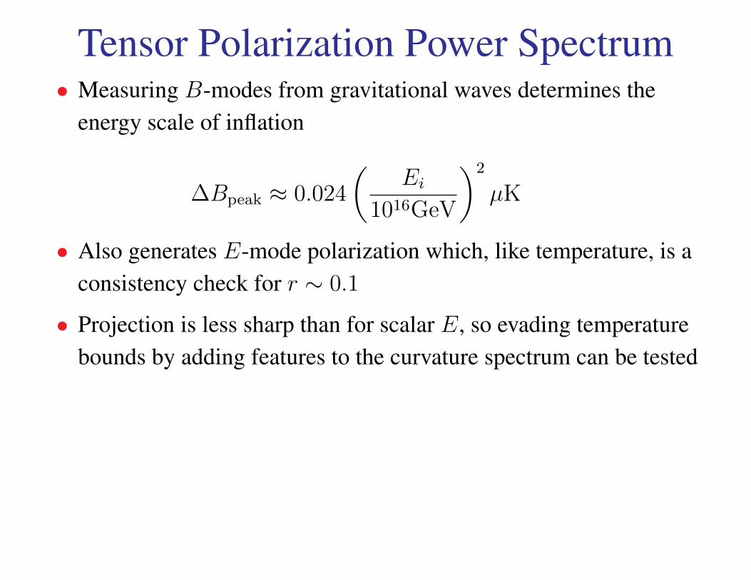
Tensor Polarization Power Spectrum• Measuring B-modes from gravitational waves determines the

energy scale of inflation

∆Bpeak ≈ 0.024

(Ei

1016GeV

)2

µK

• Also generates E-mode polarization which, like temperature, is aconsistency check for r ∼ 0.1

• Projection is less sharp than for scalar E, so evading temperaturebounds by adding features to the curvature spectrum can be tested

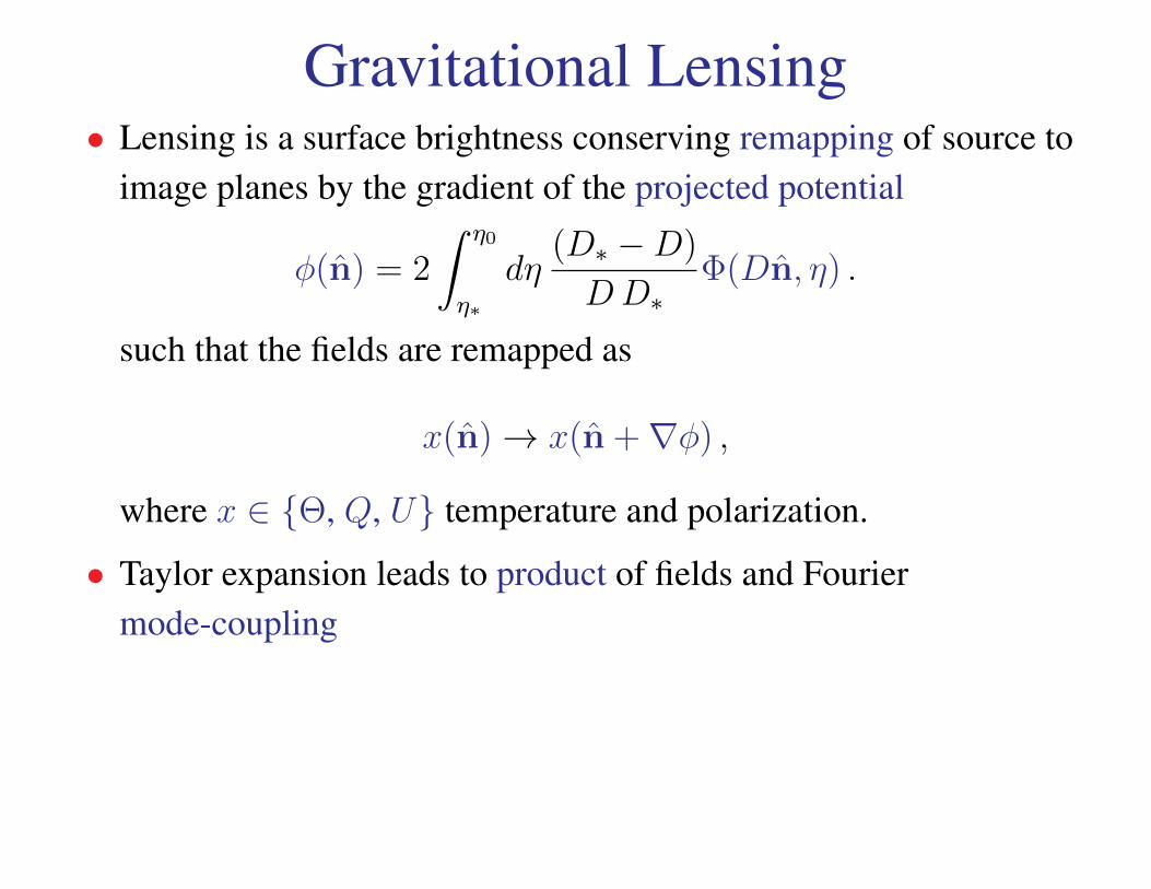
Gravitational Lensing• Lensing is a surface brightness conserving remapping of source to

image planes by the gradient of the projected potential

φ(n) = 2

∫ η0

η∗

dη(D∗ −D)

DD∗Φ(Dn, η) .

such that the fields are remapped as

x(n)→ x(n +∇φ) ,

where x ∈ Θ, Q, U temperature and polarization.

• Taylor expansion leads to product of fields and Fouriermode-coupling

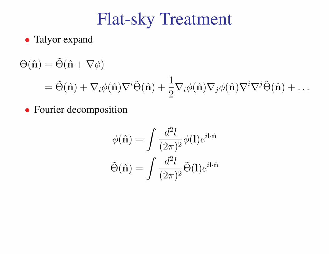
Flat-sky Treatment• Talyor expand

Θ(n) = Θ(n +∇φ)

= Θ(n) +∇iφ(n)∇iΘ(n) +1

2∇iφ(n)∇jφ(n)∇i∇jΘ(n) + . . .

• Fourier decomposition

φ(n) =

∫d2l

(2π)2φ(l)eil·n

Θ(n) =

∫d2l

(2π)2Θ(l)eil·n

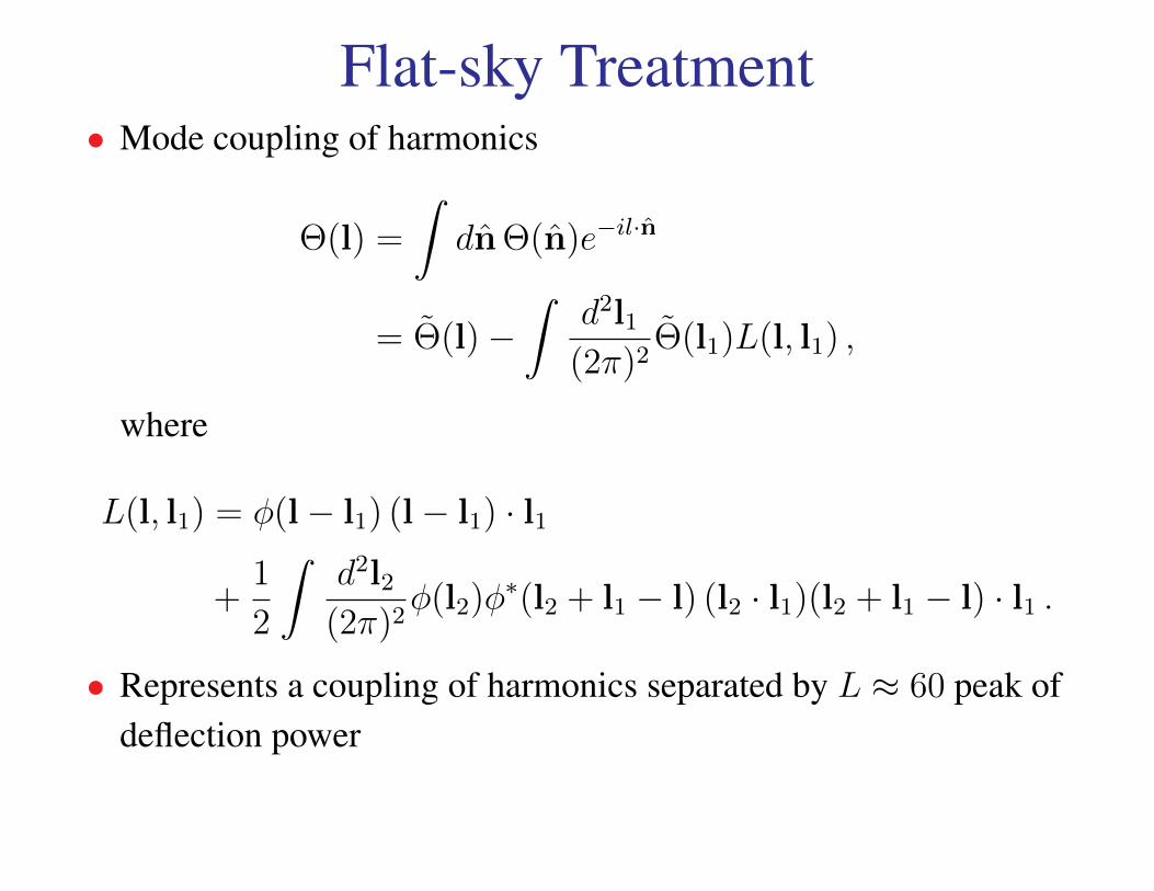
Flat-sky Treatment• Mode coupling of harmonics

Θ(l) =

∫dnΘ(n)e−il·n

= Θ(l)−∫

d2l1(2π)2

Θ(l1)L(l, l1) ,

where

L(l, l1) = φ(l− l1) (l− l1) · l1

+1

2

∫d2l2

(2π)2φ(l2)φ∗(l2 + l1 − l) (l2 · l1)(l2 + l1 − l) · l1 .

• Represents a coupling of harmonics separated by L ≈ 60 peak ofdeflection power

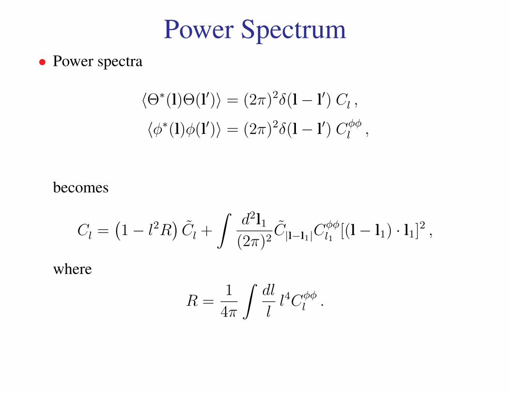
Power Spectrum• Power spectra

〈Θ∗(l)Θ(l′)〉 = (2π)2δ(l− l′) Cl ,

〈φ∗(l)φ(l′)〉 = (2π)2δ(l− l′) Cφφl ,

becomes

Cl =(1− l2R

)Cl +

∫d2l1

(2π)2C|l−l1|C

φφl1

[(l− l1) · l1]2 ,

where

R =1

4π

∫dl

ll4Cφφ

l .

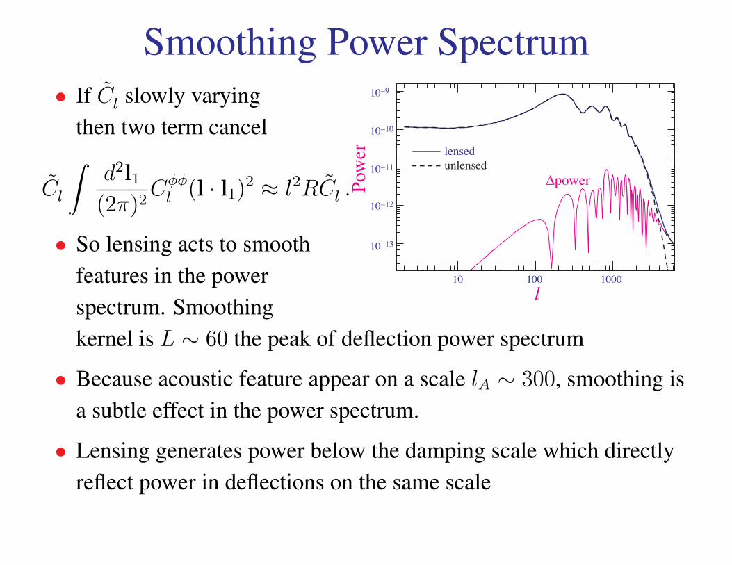
Smoothing Power Spectrum.

Pow

er

10–9

10–10

10–11

10–12

10–13

lensedunlensed

∆power

l10 100 1000

• If Cl slowly varyingthen two term cancel

Cl

∫d2l1

(2π)2Cφφl (l · l1)2 ≈ l2RCl .

• So lensing acts to smoothfeatures in the powerspectrum. Smoothingkernel is L ∼ 60 the peak of deflection power spectrum

• Because acoustic feature appear on a scale lA ∼ 300, smoothing isa subtle effect in the power spectrum.

• Lensing generates power below the damping scale which directlyreflect power in deflections on the same scale

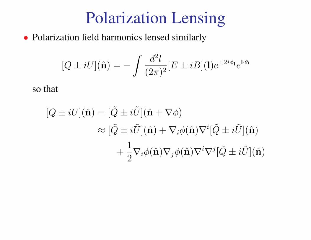
Polarization Lensing• Polarization field harmonics lensed similarly

[Q± iU ](n) = −∫

d2l

(2π)2[E ± iB](l)e±2iφlel·n

so that

[Q± iU ](n) = [Q± iU ](n +∇φ)

≈ [Q± iU ](n) +∇iφ(n)∇i[Q± iU ](n)

+1

2∇iφ(n)∇jφ(n)∇i∇j[Q± iU ](n)

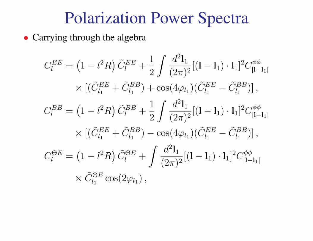
Polarization Power Spectra• Carrying through the algebra

CEEl =

(1− l2R

)CEEl +

1

2

∫d2l1

(2π)2[(l− l1) · l1]2Cφφ

|l−l1|

× [(CEEl1

+ CBBl1

) + cos(4ϕl1)(CEEl1− CBB

l1)] ,

CBBl =

(1− l2R

)CBBl +

1

2

∫d2l1

(2π)2[(l− l1) · l1]2Cφφ

|l−l1|

× [(CEEl1

+ CBBl1

)− cos(4ϕl1)(CEEl1− CBB

l1)] ,

CΘEl =

(1− l2R

)CΘEl +

∫d2l1

(2π)2[(l− l1) · l1]2Cφφ

|l−l1|

× CΘEl1

cos(2ϕl1) ,

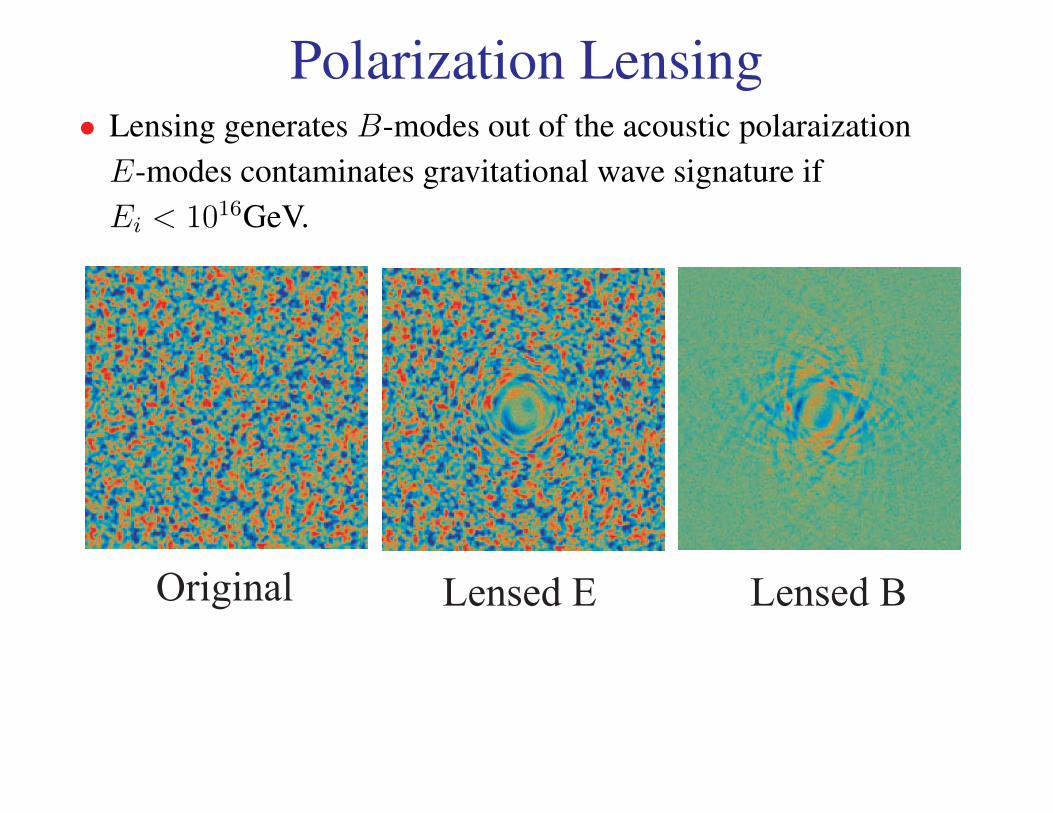
Polarization Lensing• Lensing generates B-modes out of the acoustic polaraizationE-modes contaminates gravitational wave signature ifEi < 1016GeV.

Original Lensed BLensed E

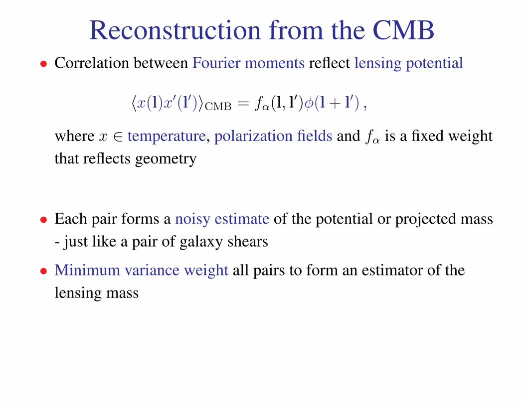
Reconstruction from the CMB• Correlation between Fourier moments reflect lensing potential

〈x(l)x′(l′)〉CMB = fα(l, l′)φ(l + l′) ,

where x ∈ temperature, polarization fields and fα is a fixed weightthat reflects geometry

• Each pair forms a noisy estimate of the potential or projected mass- just like a pair of galaxy shears

• Minimum variance weight all pairs to form an estimator of thelensing mass