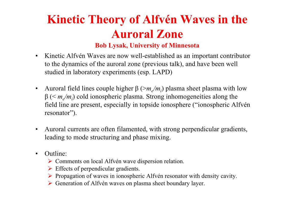
Kinetic Theory of Alfvén Waves in theAuroral Zone

Bob Lysak, University of Minnesota• Kinetic Alfvén Waves are now well-established as an important contributor

to the dynamics of the auroral zone (previous talk), and have been wellstudied in laboratory experiments (esp. LAPD)

• Auroral field lines couple higher β (>me/mi) plasma sheet plasma with lowβ (< me/mi) cold ionospheric plasma. Strong inhomogeneities along thefield line are present, especially in topside ionosphere (“ionospheric Alfvénresonator”).

• Auroral currents are often filamented, with strong perpendicular gradients,leading to mode structuring and phase mixing.

• Outline: Comments on local Alfvén wave dispersion relation. Effects of perpendicular gradients. Propagation of waves in ionospheric Alfvén resonator with density cavity. Generation of Alfvén waves on plasma sheet boundary layer.

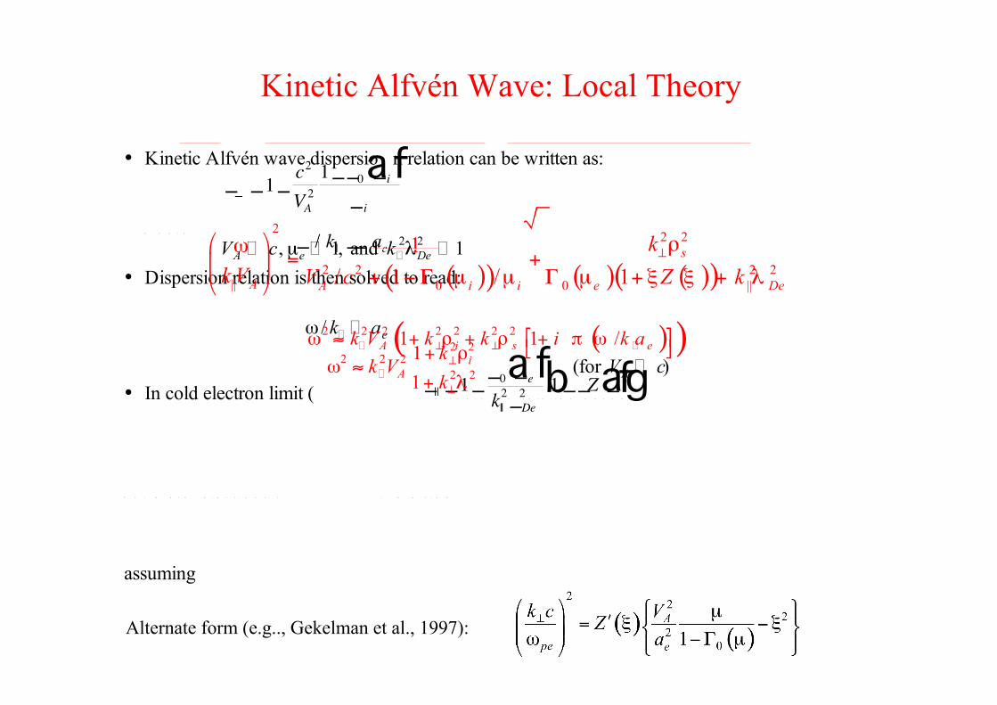
Kinetic Alfvén Wave: Local Theory

• Kinetic Alfvén wave dispersio n relation can be written as:

2

|| ||

2

|| ||

det 0! !

! !

" #$ %=& '

$ %( )

n n n

n n n

w h e r e

__

__ _ _

_1

12

2

0c

VA

i

i

_ af

__

__ _

||

||

_ _ _1 10

2 2

_e

Dek

Za f afb g

• Dispersion relation is then solved to read:

( )( ) ( ) ( )( )

22 2

2 2 2 2|| 0 0 ||

1

/ 1 / 1

!" # *+

= +& '+ % , µ µ , µ + - - + .( )

s

A A i i e De

k

k V V c Z k

• In cold electron limit (

_ /||k a

e__

) , d i s p e r s i o n r e l a t i o n b e c o m e s :

2 22 2 2

2 2

1

1(for )!

!

+ *+ /

+ .�

�A A

ik

k Vk

cV

F o r w a r m e l e c t r o n s (

/e

k a+��

) , w e f i n d

( )( )2 2 2 2 2 2 21 1 /! !

0 1+ / + * + * + 2 +3 4� �A i s ek V k k i k a

assuming

2 2, 1, and 1

A e DeV c kµ .

�� � �

.

Alternate form (e.g.., Gekelman et al., 1997):

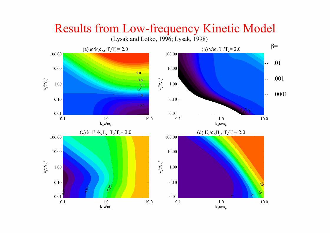
Results from Low-frequency Kinetic Model(Lysak and Lotko, 1996; Lysak, 1998)

β=

-- .01

-- .001

-- .0001

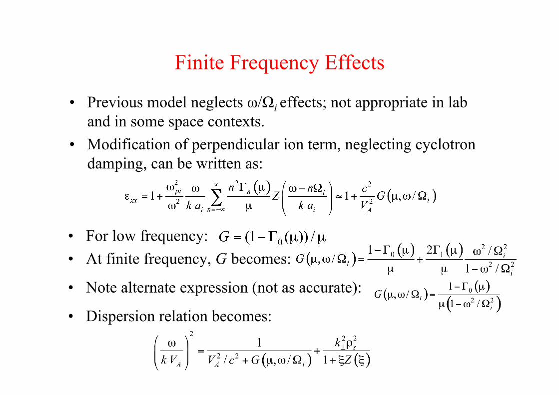
Finite Frequency Effects

• Previous model neglects ω/Ωi effects; not appropriate in laband in some space contexts.

• Modification of perpendicular ion term, neglecting cyclotrondamping, can be written as:

• For low frequency:• At finite frequency, G becomes:

• Note alternate expression (not as accurate):

• Dispersion relation becomes:

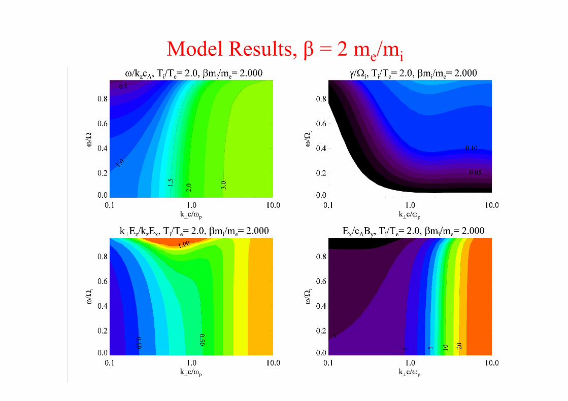
Model Results, β = 2 me/mi

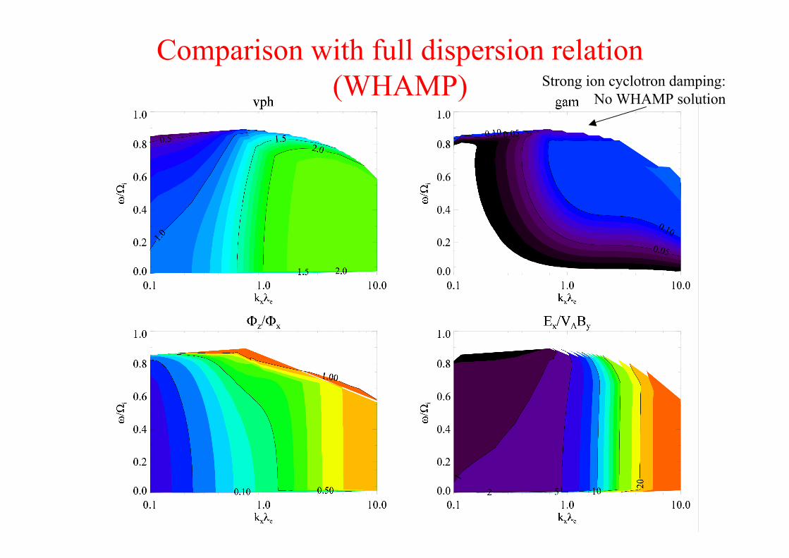
Comparison with full dispersion relation(WHAMP) Strong ion cyclotron damping:

No WHAMP solution

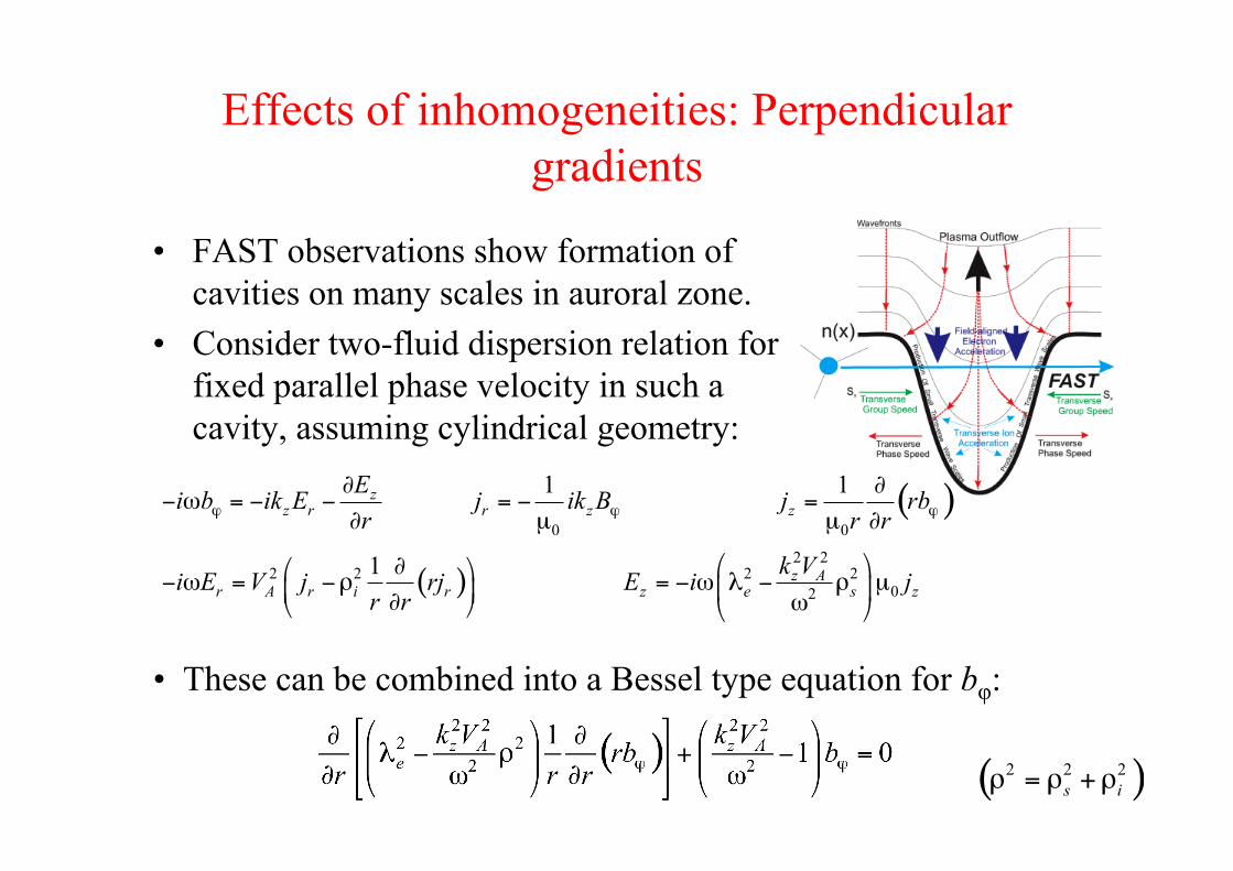
Effects of inhomogeneities: Perpendiculargradients

• FAST observations show formation ofcavities on many scales in auroral zone.

• Consider two-fluid dispersion relation forfixed parallel phase velocity in such acavity, assuming cylindrical geometry:

( )

( )

0 0

2 2

2 2 2 2

02

1 1

1

zz r r z z

z Ar A r i r z e s z

Ei b ik E j ik B j rb

r r r

k Vi E V j rj E i j

r r

! ! !

" "# $ = # # = # =

" µ µ "

% &"% &# $ = #' = # $ ( # ' µ) *) *" $+ , + ,

• These can be combined into a Bessel type equation for bφ:

( )2 2 2

s i! = ! +!

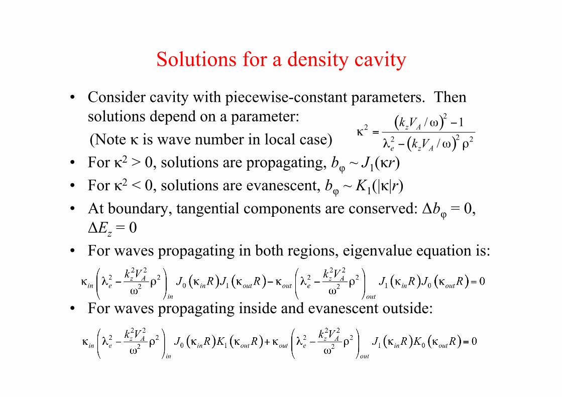
Solutions for a density cavity

• Consider cavity with piecewise-constant parameters. Thensolutions depend on a parameter:

(Note κ is wave number in local case)• For κ2 > 0, solutions are propagating, bφ ~ J1(κr)• For κ2 < 0, solutions are evanescent, bφ ~ K1(|κ|r)• At boundary, tangential components are conserved: Δbφ = 0,ΔEz = 0

• For waves propagating in both regions, eigenvalue equation is:

• For waves propagating inside and evanescent outside:

( )

( )

2

2

22 2

/ 1

/

z A

e z A

k V

k V

! "# =

$ " ! %

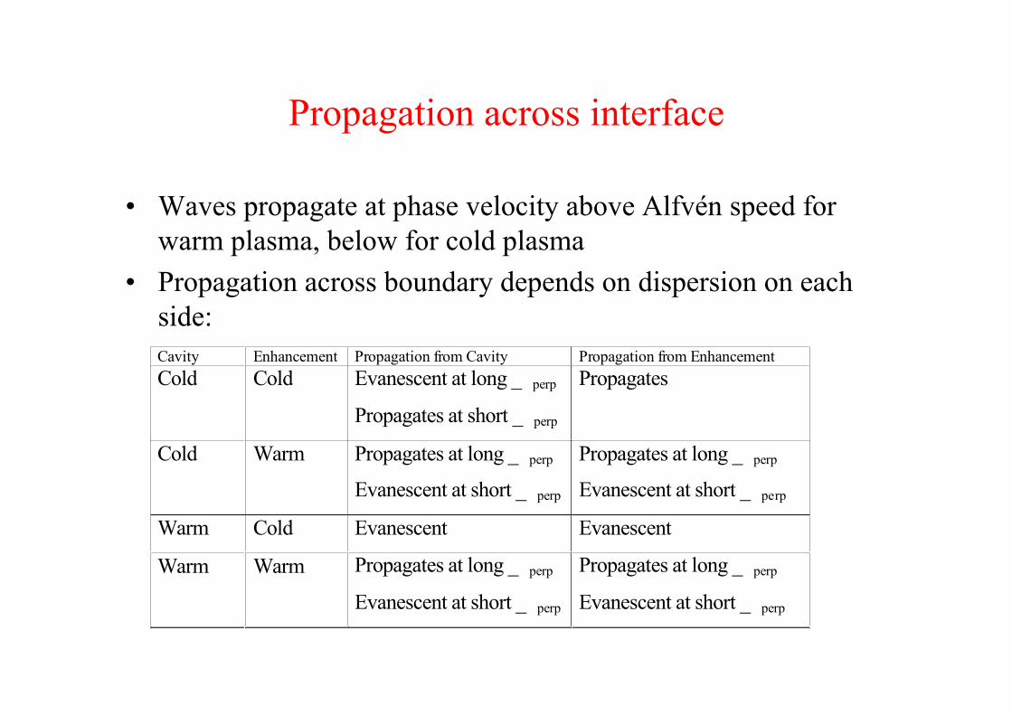
Propagation across interface

• Waves propagate at phase velocity above Alfvén speed forwarm plasma, below for cold plasma

• Propagation across boundary depends on dispersion on eachside:Cavity Enhancement Propagation from Cavity Propagation from Enhancement

Cold Cold Evanescent at long _ perp

Propagates at short _ perp

Propagates

Cold Warm Propagates at long _ perp

Evanescent at short _ perp

Propagates at long _ perp

Evanescent at short _ perp

Warm Cold Evanescent Evanescent

Warm Warm Propagates at long _ perp

Evanescent at short _ perp

Propagates at long _ perp

Evanescent at short _ perp

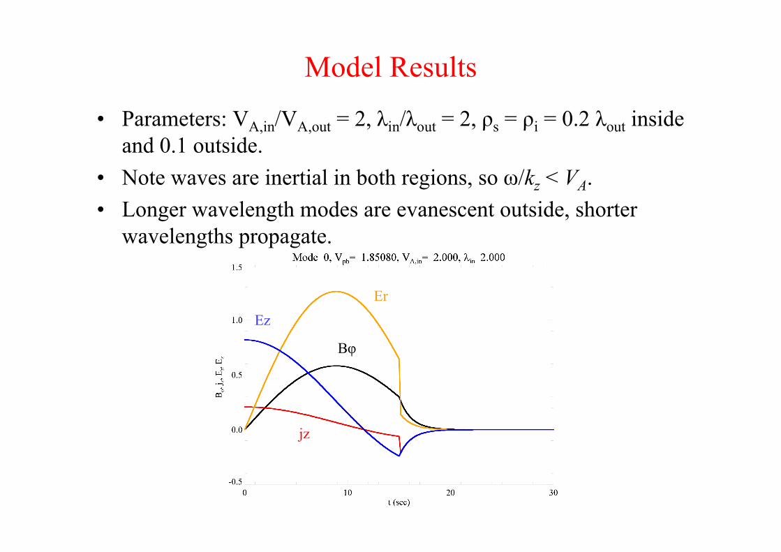
Model Results

• Parameters: VA,in/VA,out = 2, λin/λout = 2, ρs = ρi = 0.2 λout insideand 0.1 outside.

• Note waves are inertial in both regions, so ω/kz < VA.• Longer wavelength modes are evanescent outside, shorter

wavelengths propagate.

Bφ

jz

ErEz

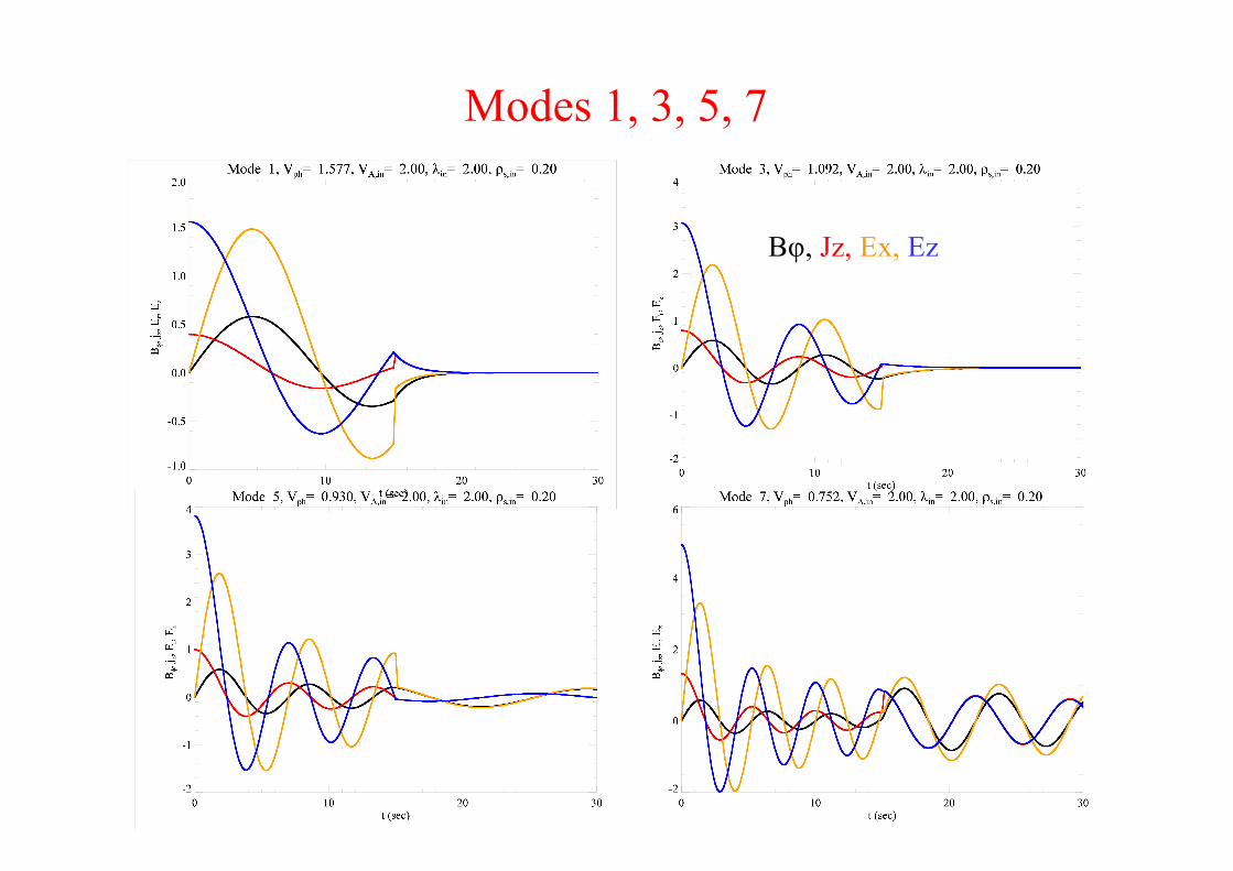
Modes 1, 3, 5, 7

Bφ, Jz, Ex, Ez

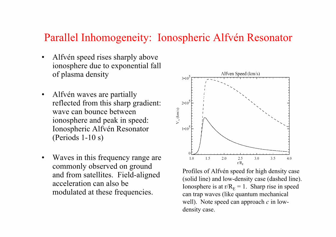
Parallel Inhomogeneity: Ionospheric Alfvén Resonator

• Alfvén speed rises sharply aboveionosphere due to exponential fallof plasma density

• Alfvén waves are partiallyreflected from this sharp gradient:wave can bounce betweenionosphere and peak in speed:Ionospheric Alfvén Resonator(Periods 1-10 s)

• Waves in this frequency range arecommonly observed on groundand from satellites. Field-alignedacceleration can also bemodulated at these frequencies.

Profiles of Alfvén speed for high density case(solid line) and low-density case (dashed line).Ionosphere is at r/RE = 1. Sharp rise in speedcan trap waves (like quantum mechanicalwell). Note speed can approach c in low-density case.

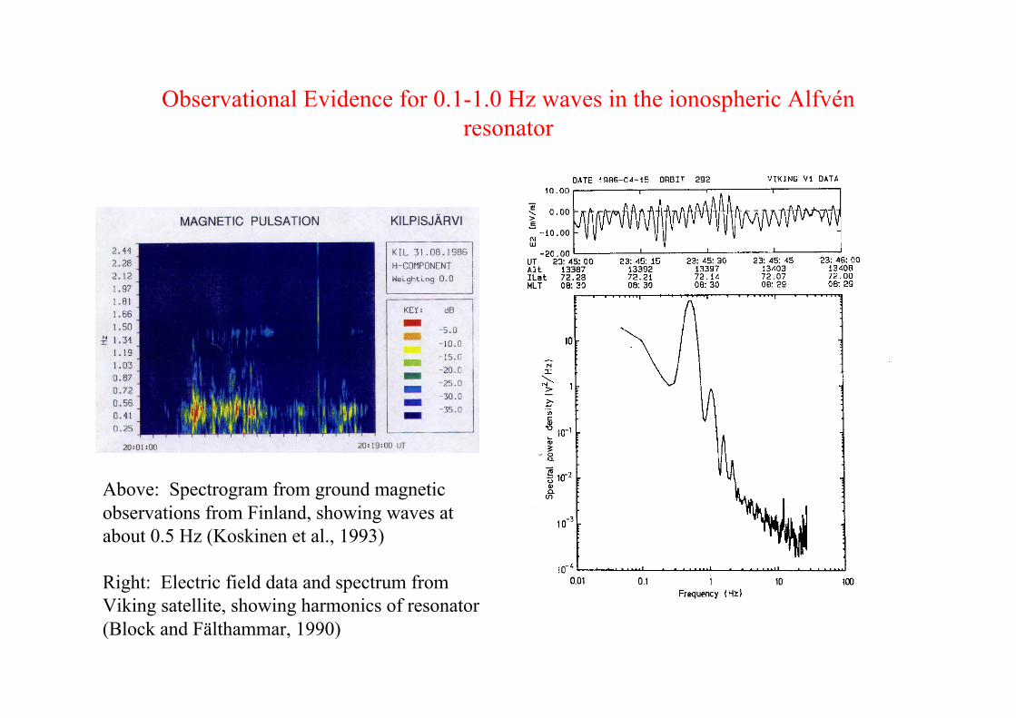
Observational Evidence for 0.1-1.0 Hz waves in the ionospheric Alfvénresonator

Above: Spectrogram from ground magneticobservations from Finland, showing waves atabout 0.5 Hz (Koskinen et al., 1993)

Right: Electric field data and spectrum fromViking satellite, showing harmonics of resonator(Block and Fälthammar, 1990)

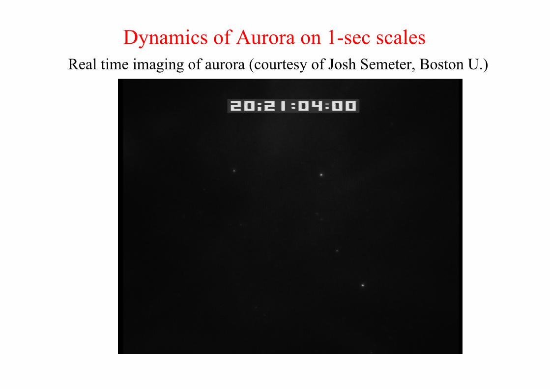
Dynamics of Aurora on 1-sec scalesReal time imaging of aurora (courtesy of Josh Semeter, Boston U.)

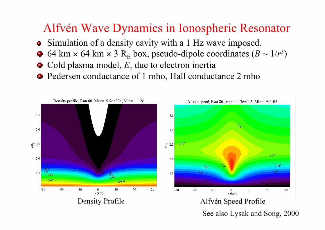
Alfvén Wave Dynamics in Ionospheric Resonator Simulation of a density cavity with a 1 Hz wave imposed. 64 km × 64 km × 3 RE box, pseudo-dipole coordinates (B ~ 1/r3) Cold plasma model, Ez due to electron inertia Pedersen conductance of 1 mho, Hall conductance 2 mho

See also Lysak and Song, 2000Density Profile Alfvén Speed Profile

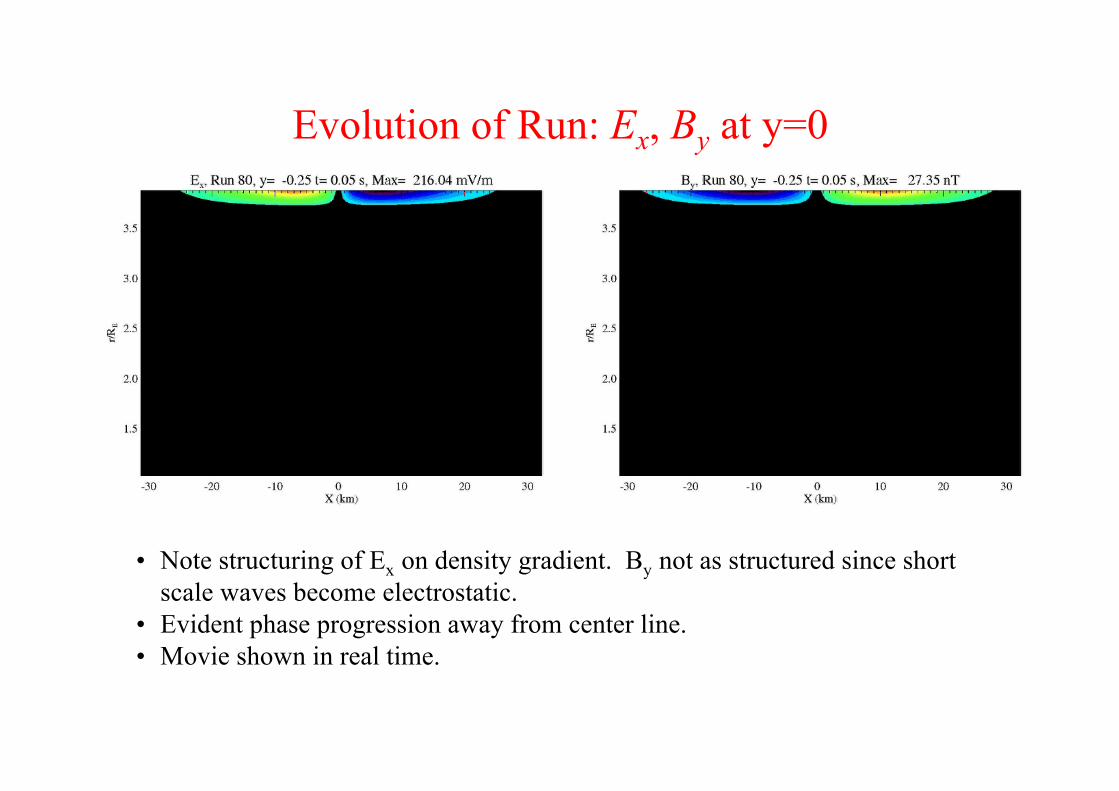
Evolution of Run: Ex, By at y=0

• Note structuring of Ex on density gradient. By not as structured since shortscale waves become electrostatic.

• Evident phase progression away from center line.• Movie shown in real time.

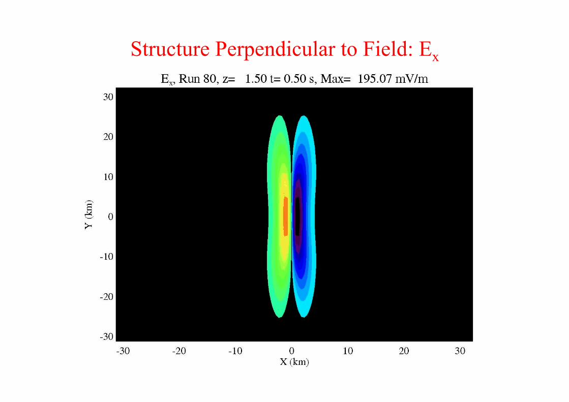
Structure Perpendicular to Field: Ex

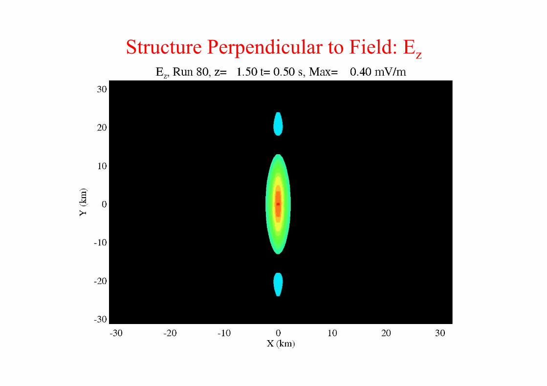
Structure Perpendicular to Field: Ez

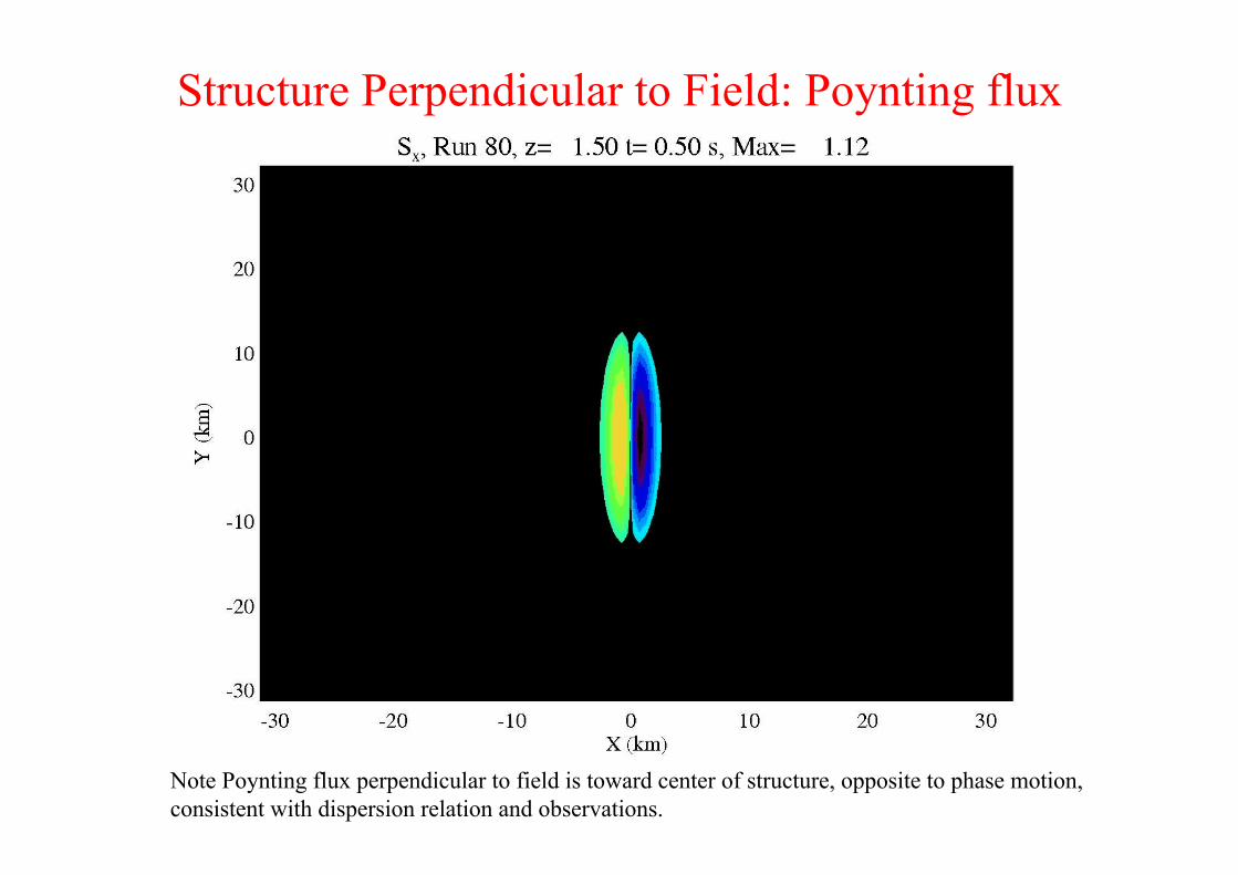
Structure Perpendicular to Field: Poynting flux

Note Poynting flux perpendicular to field is toward center of structure, opposite to phase motion,consistent with dispersion relation and observations.

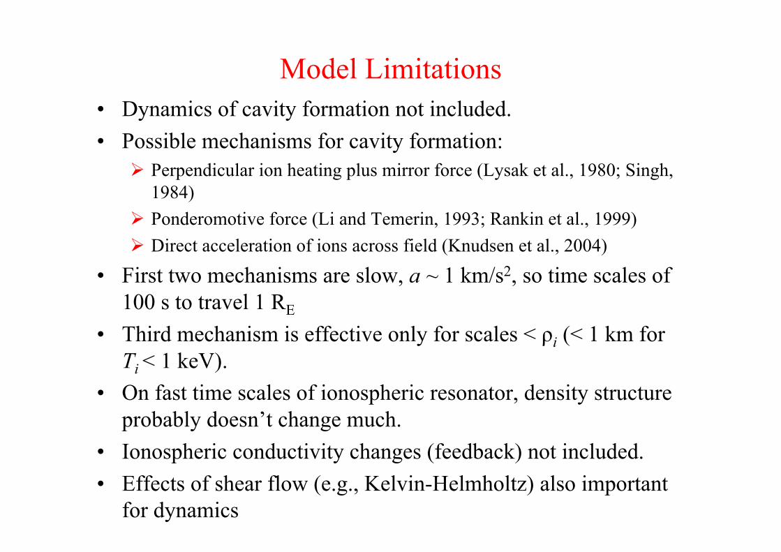
Model Limitations• Dynamics of cavity formation not included.• Possible mechanisms for cavity formation:

Perpendicular ion heating plus mirror force (Lysak et al., 1980; Singh,1984)

Ponderomotive force (Li and Temerin, 1993; Rankin et al., 1999) Direct acceleration of ions across field (Knudsen et al., 2004)

• First two mechanisms are slow, a ~ 1 km/s2, so time scales of100 s to travel 1 RE

• Third mechanism is effective only for scales < ρi (< 1 km forTi < 1 keV).

• On fast time scales of ionospheric resonator, density structureprobably doesn’t change much.

• Ionospheric conductivity changes (feedback) not included.• Effects of shear flow (e.g., Kelvin-Helmholtz) also important

for dynamics

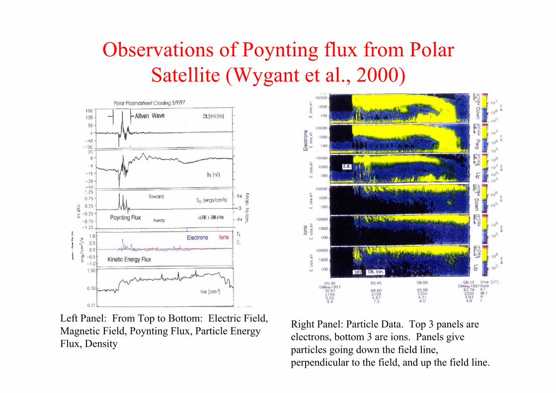
Observations of Poynting flux from PolarSatellite (Wygant et al., 2000)

Left Panel: From Top to Bottom: Electric Field,Magnetic Field, Poynting Flux, Particle EnergyFlux, Density

Right Panel: Particle Data. Top 3 panels areelectrons, bottom 3 are ions. Panels giveparticles going down the field line,perpendicular to the field, and up the field line.

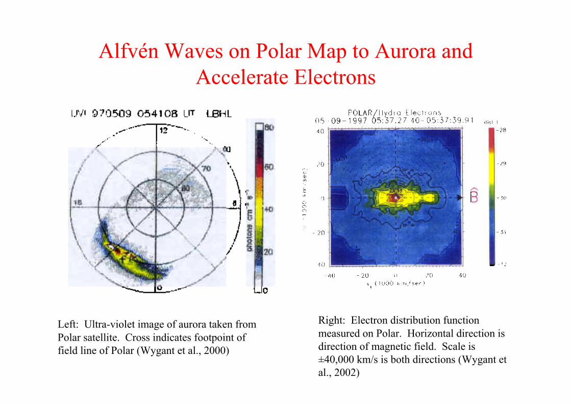
Alfvén Waves on Polar Map to Aurora andAccelerate Electrons

Left: Ultra-violet image of aurora taken fromPolar satellite. Cross indicates footpoint offield line of Polar (Wygant et al., 2000)

Right: Electron distribution functionmeasured on Polar. Horizontal direction isdirection of magnetic field. Scale is±40,000 km/s is both directions (Wygant etal., 2002)

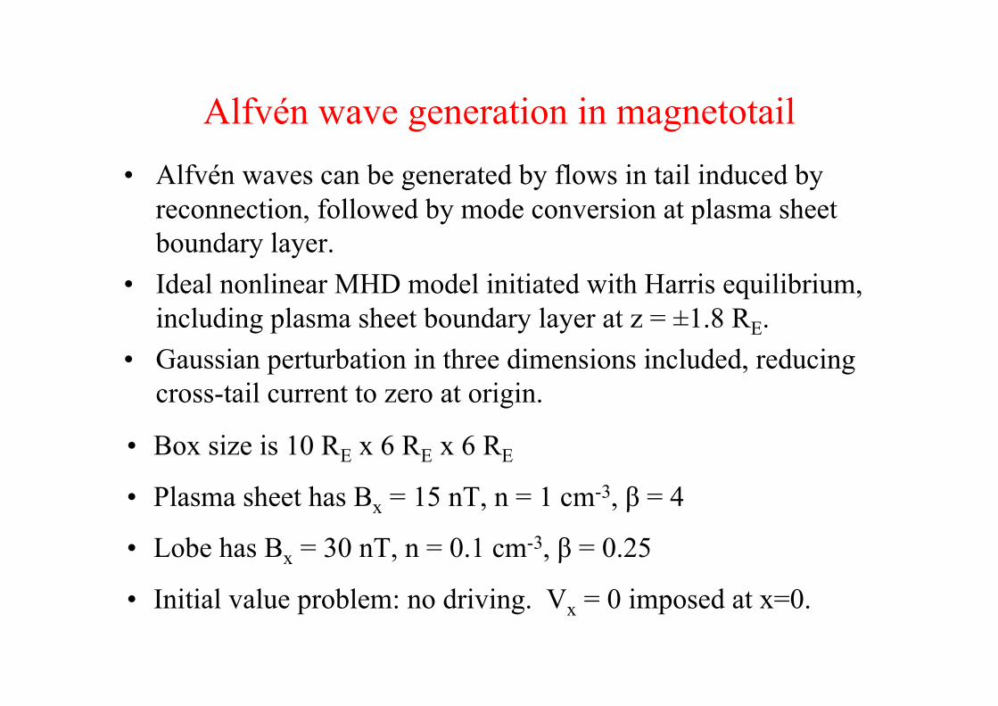
Alfvén wave generation in magnetotail• Alfvén waves can be generated by flows in tail induced by

reconnection, followed by mode conversion at plasma sheetboundary layer.

• Ideal nonlinear MHD model initiated with Harris equilibrium,including plasma sheet boundary layer at z = ±1.8 RE.

• Gaussian perturbation in three dimensions included, reducingcross-tail current to zero at origin.

• Box size is 10 RE x 6 RE x 6 RE

• Plasma sheet has Bx = 15 nT, n = 1 cm-3, β = 4

• Lobe has Bx = 30 nT, n = 0.1 cm-3, β = 0.25

• Initial value problem: no driving. Vx = 0 imposed at x=0.

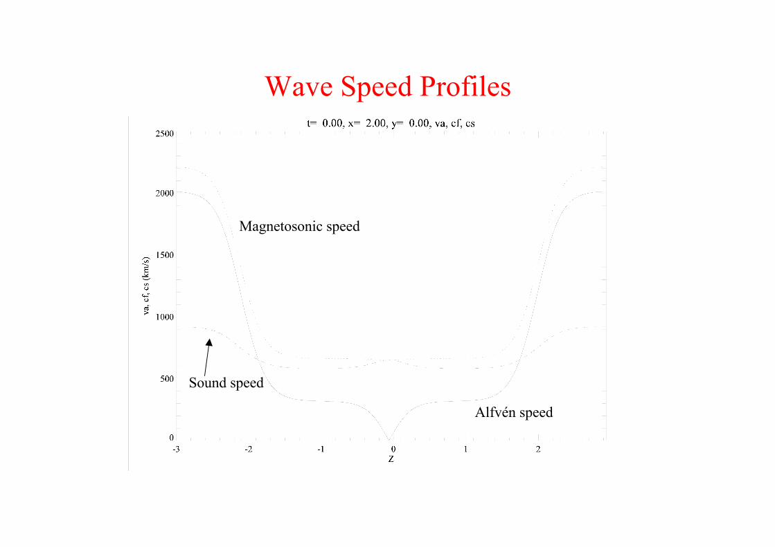
Wave Speed Profiles

Alfvén speed

Magnetosonic speed

Sound speed

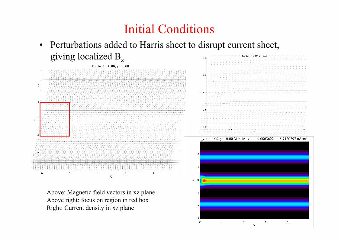
Initial Conditions• Perturbations added to Harris sheet to disrupt current sheet,

giving localized Bz

Above: Magnetic field vectors in xz planeAbove right: focus on region in red boxRight: Current density in xz plane

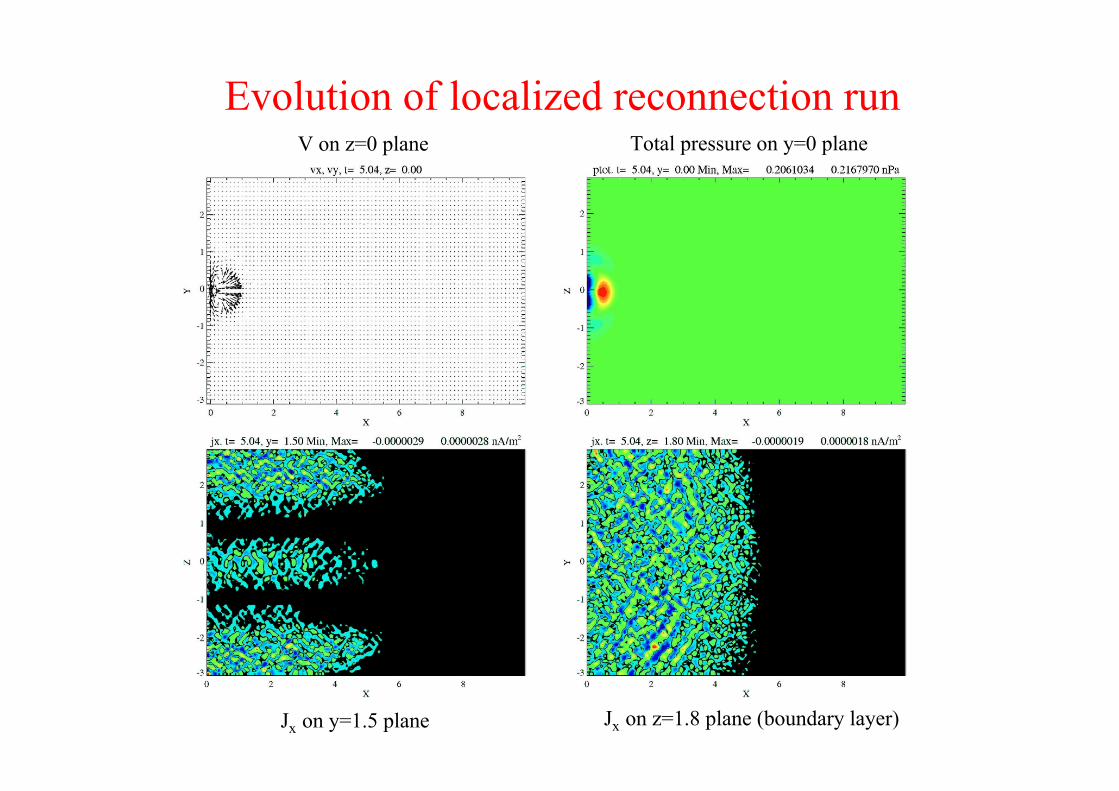
Evolution of localized reconnection runV on z=0 plane Total pressure on y=0 plane

Jx on y=1.5 plane Jx on z=1.8 plane (boundary layer)

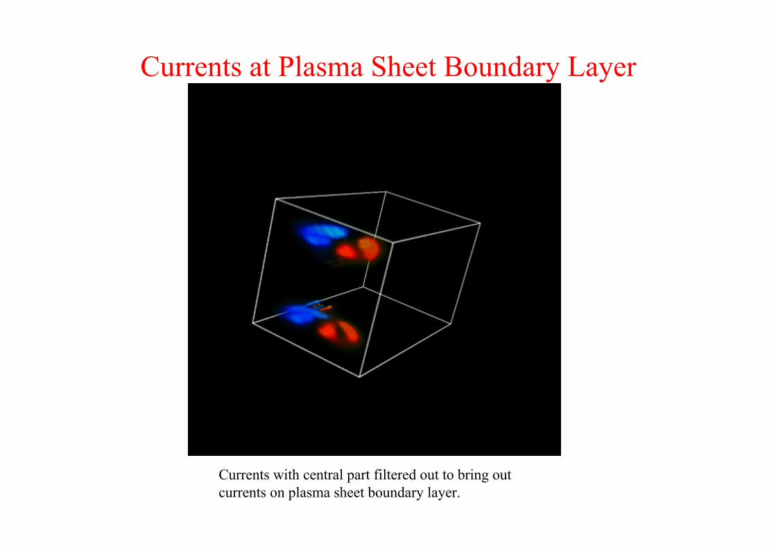
Currents at Plasma Sheet Boundary Layer

Currents with central part filtered out to bring outcurrents on plasma sheet boundary layer.

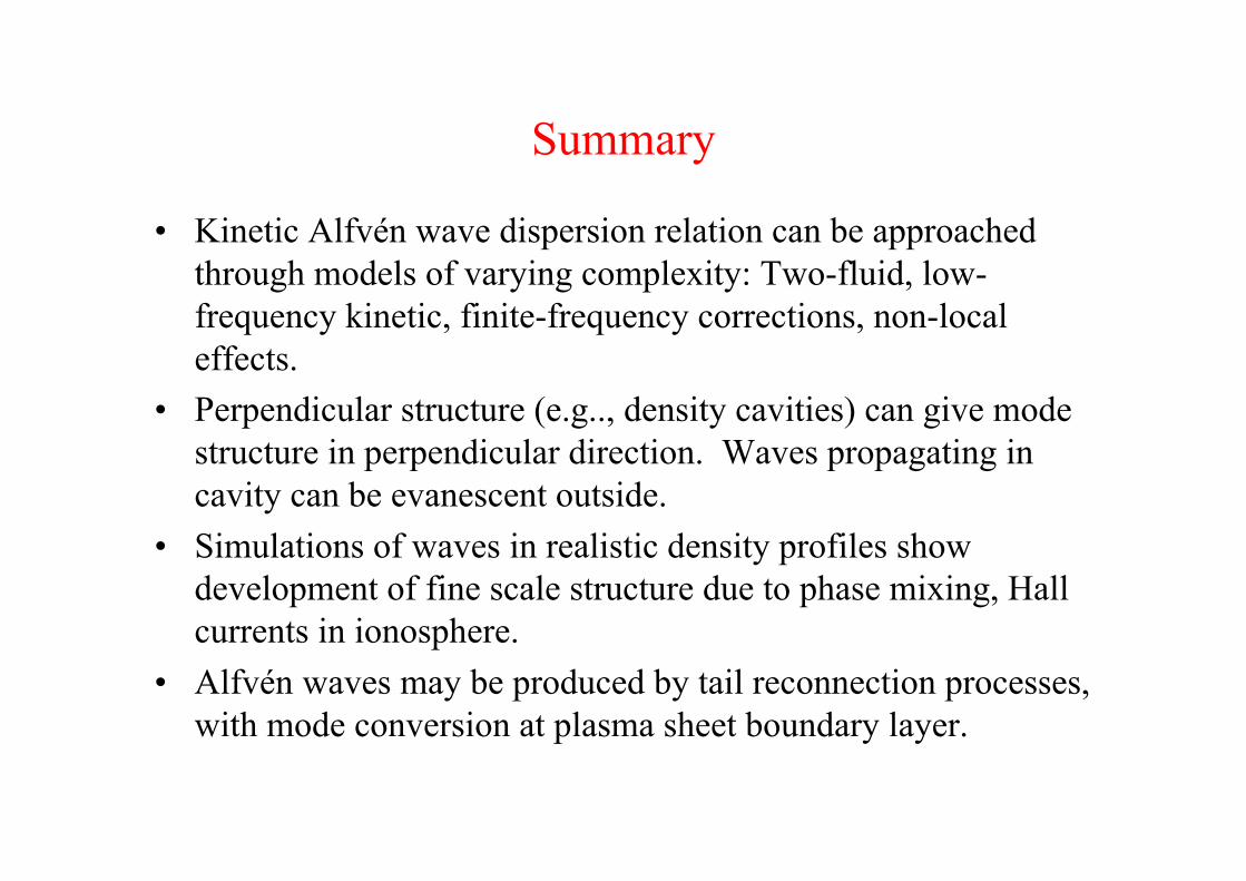
Summary

• Kinetic Alfvén wave dispersion relation can be approachedthrough models of varying complexity: Two-fluid, low-frequency kinetic, finite-frequency corrections, non-localeffects.

• Perpendicular structure (e.g.., density cavities) can give modestructure in perpendicular direction. Waves propagating incavity can be evanescent outside.

• Simulations of waves in realistic density profiles showdevelopment of fine scale structure due to phase mixing, Hallcurrents in ionosphere.

• Alfvén waves may be produced by tail reconnection processes,with mode conversion at plasma sheet boundary layer.

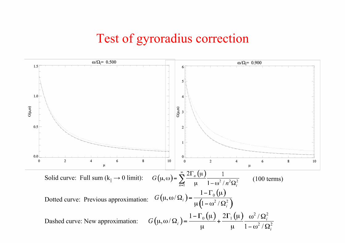
Test of gyroradius correction

Solid curve: Full sum (k|| → 0 limit):

Dotted curve: Previous approximation:

Dashed curve: New approximation:

(100 terms)

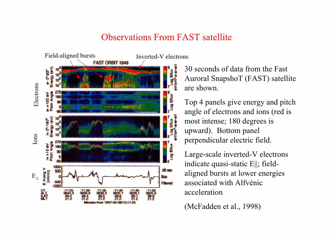
Observations From FAST satellite

30 seconds of data from the FastAuroral SnapshoT (FAST) satelliteare shown.

Top 4 panels give energy and pitchangle of electrons and ions (red ismost intense; 180 degrees isupward). Bottom panelperpendicular electric field.

Large-scale inverted-V electronsindicate quasi-static E||; field-aligned bursts at lower energiesassociated with Alfvénicacceleration

(McFadden et al., 1998)

Inverted-V electronsField-aligned bursts

Elec

trons

Ions

E⊥

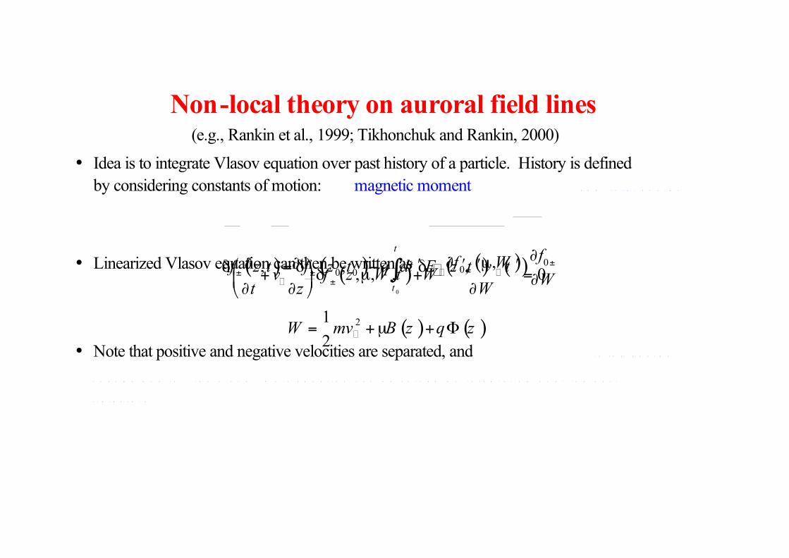
Non-local theory on auroral field lines (e.g., Rankin et al., 1999; Tikhonchuk and Rankin, 2000)

• Idea is to integrate Vlasov equation over past history of a particle. History is defined

by considering constants of motion: magnetic moment

2/ 2mv B!µ =

a n d t o t a l e n e r g y

( ) ( )21

2W mv B z q z= +µ + "

�

• Linearized Vlasov equation can then be written as

( )( )0

,, , , 0

f Wv f z W t W

t z W

±

±

# µ# #$ %+ & µ + =' (

# # #) *�

�

• Note that positive and negative velocities are separated, and

W qE v=� �

�

i s t h e e n e r g y

c h a n g e d u e t o t h e w a v e . T h i s e q u a t i o n c a n b e s o l v e d b y i n t e g r a t i n g o v e r t h e p a s t

t r a j e c t o r y

( ) ( ) ( ) ( )0

00 0, , ,

t

t

ff z t f z t q dt E z t v t

W±

± ±

#+ + + +& = & , &

#- � �

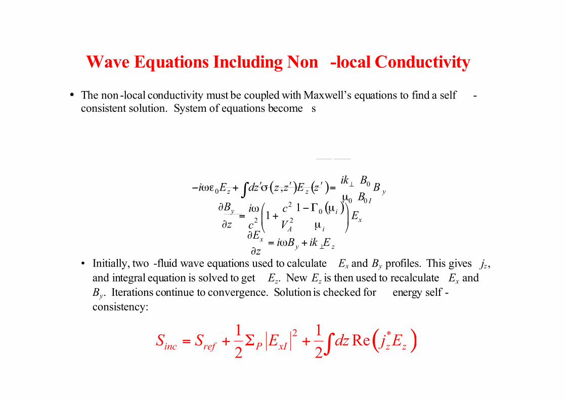
Wave Equations Including Non -local Conductivity

• The non -local conductivity must be coupled with Maxwell’s equations to find a self -consistent solution. System of equations become s

xy z

Ei B ik E

z!

"= # +

"

( )20

2 2

11

y ix

iA

B i cE

z c V

" $ %&' µ#= +( )" µ* +

( ) ( ) 00

0 0

,z z y

I

Biki E dz z z E z B

B

!, , ,& #- + . =µ/

• Initially, two -fluid wave equations used to calculate Ex and By profiles. This gives jz,

and integral equation is solved to get Ez. New Ez is then used to recalculate Ex and

By. Iterations continue to convergence. Solution is checked for energy self -

consistency:

( )2 *1 1Re

2 2inc ref P xI z zS S E dz j E= + ! + "

Non-local conductivity kernel• Integration of Vlasov equation leads to the conductivity:

Upgoing ionosphere elec.

Downgoing magnetospheric elec.

Mirroring magnetospheric elec.

Note here

( )( )

( ) ( )

( ) ( ) ( ) ( ) ( )( )

( ) ( )

( ) ( ) ( ) ( ) ( )( )

1

1

0

0

0

0

1

2,0

2

0

, , ,0

,0

0

, , ,0

2,

I

m m

m m

i z zI

e

i z z i z z i z zIm

i z zM

e

i z z i z z i z zMm

q B z fz z dW z z d e

Wm

fd z z e z z e

W

fdW z z d e

W

fd z z e z z e

W

µ!"#$

% &

µ" "#$ + #$ #$

µ

µ!"#$

% &

µ" "#$ + #$ #$

µ

' () *+" ", = % - % µ./

*.+ 01

2*"% µ- % %- % 3

* 34

( *"+ - % µ.

*.0

2*"% µ- % %- %

*

5 5

5

5 5

5

( ) ( )max max

min min

2sin sin

W

T B

n BW

f idW d n z n z

W n

µ !

=%!µ

334

6* # +"+ µ 7 7 8

) * #% # +9:5 5

Reflected ionospheric elec.

Trapped electrons

( )( )

( )( )0 1min , min

z z z z

W U z W U z

B z B z! !> <

! !" "µ = µ =

! !

and Wmin,, Wmax, µmin and µmax give boundary of trapped region

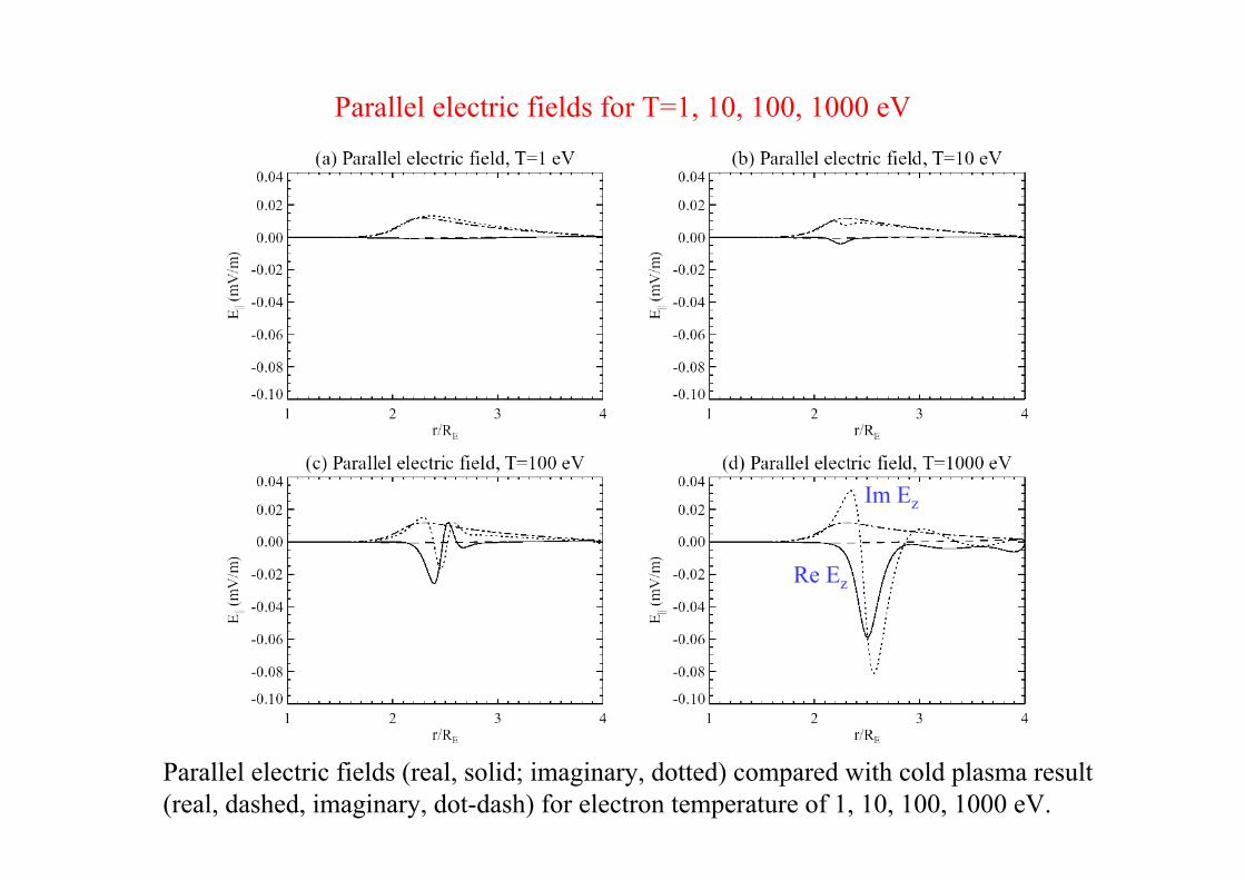
Parallel electric fields for T=1, 10, 100, 1000 eV

Parallel electric fields (real, solid; imaginary, dotted) compared with cold plasma result(real, dashed, imaginary, dot-dash) for electron temperature of 1, 10, 100, 1000 eV.

Re Ez

Im Ez