Kinetic Magneto-Hydro-Dynamics (MHD) · Kinetic Magneto-Hydro-Dynamics (MHD) 3 2.4. Perpendicular...
18
DRAFT 1 Kinetic Magneto-Hydro-Dynamics (MHD) Felix I. Parra Rudolf Peierls Centre for Theoretical Physics, University of Oxford, Oxford OX1 3NP, UK (This version is of 1 March 2019) 1. Introduction In these notes, we consider a magnetized plasma (ρ s* 1 and ω/Ω s 1 for all species s) with magnetic energy of the order of the thermal energy, β = 2μ 0 p B 2 ∼ 1. (1.1) Thus, the plasma has sufficient energy to modify the background magnetic field. To simplify the derivation as much as possible, we know consider the high flow regime, where E ⊥ ∼ v ti B ∼ 1 ρ i* T eL (1.2) and E k ∼ T eL . (1.3) In this regime, we will obtain a model that is the kinetic equivalent of Magneto-Hydro- Dynamics (MHD). 2. Kinetic Magneto-Hydro-Dynamics To determine the state of the plasma, we need to evolve in time the distribution functions f s (r, v,t) for all species s, the magnetic field B(r,t) and the electric field E(r,t). To evolve the electric field, we split it into its parallel component, E k , small by a factor of ρ i* 1, and E ⊥ . The perpendicular component E ⊥ determines the E × B drift, v E = 1 B E × ˆ b, (2.1) so instead of E ⊥ , we can evolve in time v E . Thus, we look for equations to determine f s , B, E k and v E . These equations are • the high flow drift kinetic equation for f s , • Faraday’s induction law for B, • the quasineutrality equation for E k , and • the perpendicular momentum conservation equation for v E . 2.1. High flow drift kinetic equation For f s (r, v,t) we can use the drift kinetic equation. To lowest order in the expansion in ρ s* 1, we know that the distribution function is approximately independent of gy- rophase, f s (r,v k , μ, ϕ, t) ’hf s i ϕ (r,v k , μ, t). The equation for the gyrophase independent
Transcript of Kinetic Magneto-Hydro-Dynamics (MHD) · Kinetic Magneto-Hydro-Dynamics (MHD) 3 2.4. Perpendicular...
DRAFT 1
Kinetic Magneto-Hydro-Dynamics (MHD)
Felix I. Parra
Rudolf Peierls Centre for Theoretical Physics, University of Oxford, Oxford OX1 3NP, UK
(This version is of 1 March 2019)
1. Introduction
In these notes, we consider a magnetized plasma (ρs∗ 1 and ω/Ωs 1 for all speciess) with magnetic energy of the order of the thermal energy,
β =2µ0p
B2∼ 1. (1.1)
Thus, the plasma has sufficient energy to modify the background magnetic field.To simplify the derivation as much as possible, we know consider the high flow regime,
where
E⊥ ∼ vtiB ∼1
ρi∗
T
eL(1.2)
and
E‖ ∼T
eL. (1.3)
In this regime, we will obtain a model that is the kinetic equivalent of Magneto-Hydro-Dynamics (MHD).
2. Kinetic Magneto-Hydro-Dynamics
To determine the state of the plasma, we need to evolve in time the distributionfunctions fs(r,v, t) for all species s, the magnetic field B(r, t) and the electric fieldE(r, t). To evolve the electric field, we split it into its parallel component, E‖, small bya factor of ρi∗ 1, and E⊥. The perpendicular component E⊥ determines the E × Bdrift,
vE =1
BE× b, (2.1)
so instead of E⊥, we can evolve in time vE . Thus, we look for equations to determine fs,B, E‖ and vE . These equations are• the high flow drift kinetic equation for fs,• Faraday’s induction law for B,• the quasineutrality equation for E‖, and• the perpendicular momentum conservation equation for vE .
2.1. High flow drift kinetic equation
For fs(r,v, t) we can use the drift kinetic equation. To lowest order in the expansion inρs∗ 1, we know that the distribution function is approximately independent of gy-rophase, fs(r, v‖, µ, ϕ, t) ' 〈fs〉ϕ(r, v‖, µ, t). The equation for the gyrophase independent
2 Felix I. Parra
piece of the distribution function is
∂〈fs〉ϕ∂t
+ (v‖b + vE) · ∇〈fs〉ϕ +
[Zse
ms
(b +
1
Ωsb× Db
Dt
)·E− µb · ∇B
]∂〈fs〉ϕ∂v‖
= 0,
(2.2)where we have defined the operator
D
Dt=
∂
∂t+ (v‖b + vE) · ∇. (2.3)
We can rewrite equation (2.2) such that E‖ and vE appear instead of E,
∂〈fs〉ϕ∂t
+ (v‖b + vE) · ∇〈fs〉ϕ +
(Zse
msE‖ +
Db
Dt· vE − µb · ∇B
)∂〈fs〉ϕ∂v‖
= 0. (2.4)
We will use this equation instead of (2.2).The approximation fs(r, v‖, µ, ϕ, t) ' 〈fs〉ϕ(r, v‖, µ, t) implies that the average flow is
us ' us‖b + vE , (2.5)
where
us‖ =1
ns
∫fsv‖ d3v =
2π
ns
∫B〈fs〉ϕv‖ dv‖ dµ. (2.6)
2.2. Faraday’s induction law
Due to the orderings (1.2) and (1.3), we find that
E + vE ×B = E‖b ' 0. (2.7)
Note that according to (2.5), this equation is equivalent to E+us×B ' 0, which is oneof the MHD equations.
Taking the curl of (2.7) and using Faraday’s induction law ∇×E = −∂B/∂t, we obtain
∂B
∂t= ∇× (vE ×B). (2.8)
The initial condition for B, B(r, t = 0) = B0(r), must satisfy ∇ ·B0 = 0. Equation (2.8)ensures that if ∇ ·B = 0 is satisfied at t = 0, it is satisfied at all times.
2.3. Quasineutrality equation
We start from Gauss’ law
ε0∇ ·E =∑
s
Zsens. (2.9)
Using (1.2), we find that the electric field term is of order
ε0∇ ·Eene
∼ vti
c√β
λDL, (2.10)
where λD =√ε0Te/e2ne is the Debye length. Thus, the electric field term is negligible
if the Debye length is smaller than L and the velocity vti/√β is not relativistic (we will
see that the Alfven speed vA ∼ vti/√β is the speed of propagation of perturbation in the
magnetic field). With these assumptions, we finally obtain the quasineutrality equation
∑
s
Zsens =∑
s
Zse
∫2πB〈fs〉ϕ dv‖ dµ = 0. (2.11)
Kinetic Magneto-Hydro-Dynamics (MHD) 3
2.4. Perpendicular momentum conservation equation
According to (2.5), the perpendicular component of the average velocity of species s isvE . Thus, all species move at the same perpendicular velocity vE . We can calculate thatvelocity using the perpendicular momentum equation. We multiply the Vlasov equation
∂fs∂t
+ v · ∇fs +Zse
ms(E + v ×B) · ∇vfs = 0 (2.12)
by msv and we integrate over velocity space to find the momentum conservation equationfor species s,
nsms
(∂us∂t
+ us · ∇us)
= −∇ ·Ps + ZsensE + Zsensus ×B. (2.13)
Here the pressure tensor is
Ps =
∫fsms(v − us)(v − us) d3v. (2.14)
So far, we have not used the assumption ρs∗ 1. We use it to simplify Ps. Since usis given by (2.5) to lowest order, and fs ' 〈fs〉ϕ, we can write
Ps '∫B〈fs〉ϕms[(v‖ − us‖)b + w⊥][(v‖ − us‖)b + w⊥] dv‖ dµdϕ, (2.15)
where
w⊥ =√
2µB(cosϕ e1 − sinϕ e2). (2.16)
Integrating first over ϕ, we obtain
Ps ' 2π
∫B〈fs〉ϕms[(v‖ − us‖)2bb + µB(I− bb)] = ps‖bb + ps⊥(I− bb), (2.17)
where we have used that e1e1 + e2e2 = I− bb. The quantities ps‖ =∫
2πB〈fs〉ϕms(v‖−us‖)2 dv‖ dµ and ps⊥ =
∫2πB2〈fs〉ϕmsµdv‖ dµ are known as parallel and perpendicular
pressures.Using the result for Ps in (2.17), and employing
∇ ·Ps = ∇ · [ps⊥I + (ps‖ − ps⊥)bb] = ∇ps⊥ + bb · ∇(ps‖ − ps⊥)
+(ps‖ − ps⊥)(∇ · b)b + (ps‖ − ps⊥)b · ∇b, (2.18)
we find that the parallel and perpendicular components of (2.13) are
nsms
(∂us∂t
+ us · ∇us)· b = −b · ∇ps‖ + (ps⊥ − ps‖)∇ · b + ZsensE‖ (2.19)
and
nsms
(∂us∂t
+ us · ∇us)
⊥= −∇⊥ps⊥+(ps⊥−ps‖)κ+ZsensE⊥+Zsensus×B. (2.20)
Equation (2.19) is an identity because it can be deduced from the conservative form of thedrift kinetic equation (2.4), as we showed in the notes about the drift kinetic equation.Thus, only (2.20) contains new information. In fact, the sum over all species of (2.20)gives the equation for vE . Summing over species, we obtain
∑
s
nsms
(∂us∂t
+ us · ∇us)
⊥=
*
0 due to quasineutrality∑
s
ZsensE⊥ −∇⊥P⊥ + (P⊥ − P‖)κ + J×B, (2.21)
4 Felix I. Parra
where P‖ =∑s ps‖, P⊥ =
∑s ps⊥ and J =
∑s Zsensus is the current density. To
see that equation (2.21) gives the time evolution of vE , we use us ' us‖b + vE and
b · ∂vE/∂t+ vE · ∂b/∂t = 0 = ∇vE · b +∇b · vE to write
(∂us∂t
+ us · ∇us)
⊥=∂vE∂t
+ us · ∇vE + vE ·(∂b
∂t+ us · ∇b
)b
+ us‖
(∂b
∂t+ us · ∇b
), (2.22)
Equation (2.21) for the total perpendicular momentum of the plasma can also beobtained using the drift kinetic formalism. Equation (2.21) can be understood as anequation for the perpendicular component of the current density,
J⊥ =1
Bb×
[∑
s
nsms
(∂us∂t
+ us · ∇us)]
+1
Bb×∇P⊥ +
P‖ − P⊥B
b× κ. (2.23)
This same result could be obtained from drift kinetics,
J⊥ =∑
s
Zse
∫fsv⊥ d3v =
∑
s
Zse
∫Bfs(w⊥ + vE) dv‖ dµdϕ
=∑
s
Zse
∫Bfsw⊥ dv‖ dµdϕ+
∑
s
:0 due to quasineutrality
ZsensvE
=∑
s
Zse
∫2πB〈fsw⊥〉ϕ dv‖ dµ '
∑
s
Zse
∫2πB〈fs,1w⊥〉ϕ dv‖ dµ. (2.24)
Using the lowest order gyrophase dependent piece fs,1, we find (2.23).
We need to close (2.21) by finding an equation for J. We use Ampere’s law,
∇×B = µ0
(J + ε0
∂E
∂t
). (2.25)
Here ε0 is the vacuum permittivity and µ0 is the vacuum permeability. From Ampere’slaw we can solve for J, J = (∇×B)/µ0−ε0(∂E/∂t). Using this expression for J in (2.21),and employing the usual manipulation to find Maxwell’s stress,
(∇×B)×B = B · ∇B−∇B ·B = B2κ−∇⊥(B2
2
), (2.26)
we finally obtain
∑
s
nsms
(∂us∂t
+ us · ∇us)
⊥︸ ︷︷ ︸∼ pL
= −∇⊥(B2
2µ0+ P⊥
)+
(B2
µ0+ P⊥ − P‖
)κ
︸ ︷︷ ︸∼ B2
µ0L∼ pL
+ ε0B×∂E
∂t︸ ︷︷ ︸∼ v
2tic2
B2
µ0L
. (2.27)
For the order of magnitude estimates, we have used β ∼ 1. Note that for non-relativistic
Kinetic Magneto-Hydro-Dynamics (MHD) 5
plasmas (vti/c 1), equation (2.27) becomes
∑
s
nsms
(∂us∂t
+ us · ∇us)
⊥= −∇⊥
(B2
2µ0+ P⊥
)+
(B2
µ0+ P⊥ − P‖
)κ, (2.28)
where the term in the left side of the equation can be evaluated using equation (2.22).Note that the pressure force due to the plasma takes the same form as the J×B force:
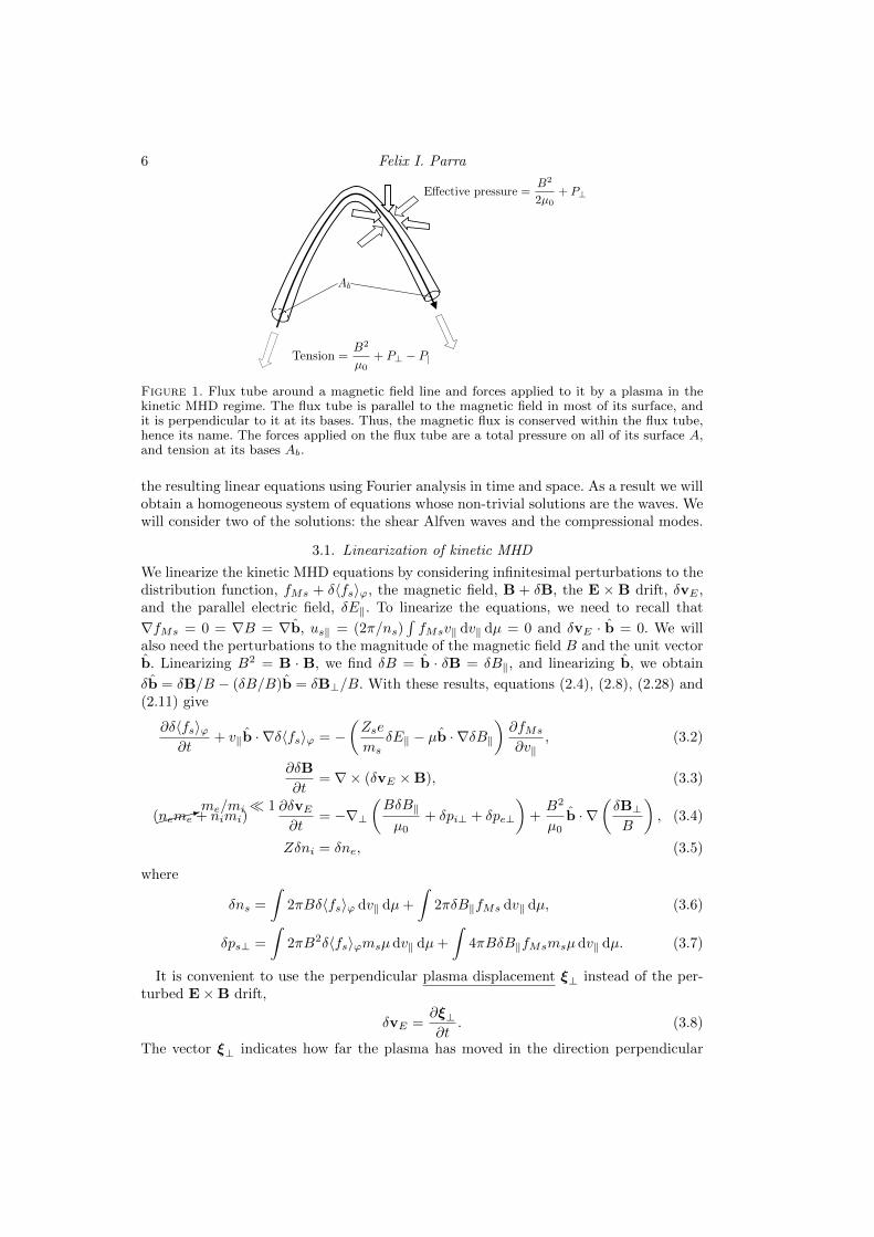
part of it is in the direction of a perpendicular gradient, and the other is in the directionof the curvature κ. In figure 1 we consider a flux tube around a magnetic field line. Theflux tube is parallel to the magnetic field in most of its surface, and it is perpendicular toit at its bases. Integrating equation (2.13) over the volume of the flux tube and summingover all species, we find
∂
∂t
(∑
s
∫
V
nsmsus d3r
)+∑
s
∫
A
nsms(us · n)us d2A =
−∑
s
∫
A
Ps · nd2A+
∫
V
J×B d3r, (2.29)
where V is the volume of the flux tube, A is the area of its boundary surface, and n isthe normal to that surface pointing outwards of the flux tube. The left side of equation(2.29) is the change of total momentum in the flux tube, and the right side is the force
on the flux tube, F. We use (2.17) and (2.26) to write∑sPs = P⊥I+ (P‖ −P⊥)bb and
J×B = ∇ · [(B2/µ0)bb− (B2/2µ0)I]. We use these results and the fact that the bases
of the flux tube, Ab, are perpendicular to the magnetic field, (b · n)b = n, to rewrite theright side of equation (2.29) as
F =
∫
A
(B2
2µ0+ P⊥
︸ ︷︷ ︸Effective pressure
)(−n) d2A+
∫
Ab
(B2
µ0+ P⊥ − P‖
︸ ︷︷ ︸Tension
)nd2A. (2.30)
Thus, we find that the forces are the ones depicted in figure 1: an effective pressure againstthe whole of the surface of the flux tube, and a tension at the bases. In the limit of theflux tube becoming infinitely short, the tension force becomes the term proportional toκ in (2.28).
3. Alfven waves and compressional modes in kinetic MHD
Low frequency (ω Ωs) perturbations to the magnetic field (generated, for example,by an antenna) propagate as Alfven waves and compressional modes. We study thispropagation in a simple system: a uniform, constant plasma composed of an ion speciesof charge Ze and mass mi and electrons of charge −e and mass me in a uniform, constantmagnetic field B = Bz. The gyroaveraged distribution function of both ions and electronsis assumed to be a Maxwellian,
〈fs〉ϕ(v‖, µ,B) = fMs(v‖, µ) ≡ ns(ms
2πTs
)3/2
exp
(−ms(v
2‖/2 + µB)
Ts
), (3.1)
where the densities ns and the temperatures Ts are constants. The densities satisfyquasineutrality, Zni = ne. We assume the equilibrium electric field to be negligible, thatis, vE = 0 and E‖ = 0.
To study the waves that propagate in this system, we first linearize and we then solve
6 Felix I. Parra
E↵ective pressure =B2
2µ0+ P?
Tension =B2
µ0+ P? Pk
Ab
Figure 1. Flux tube around a magnetic field line and forces applied to it by a plasma in thekinetic MHD regime. The flux tube is parallel to the magnetic field in most of its surface, andit is perpendicular to it at its bases. Thus, the magnetic flux is conserved within the flux tube,hence its name. The forces applied on the flux tube are a total pressure on all of its surface A,and tension at its bases Ab.
the resulting linear equations using Fourier analysis in time and space. As a result we willobtain a homogeneous system of equations whose non-trivial solutions are the waves. Wewill consider two of the solutions: the shear Alfven waves and the compressional modes.
3.1. Linearization of kinetic MHD
We linearize the kinetic MHD equations by considering infinitesimal perturbations to thedistribution function, fMs + δ〈fs〉ϕ, the magnetic field, B + δB, the E × B drift, δvE ,and the parallel electric field, δE‖. To linearize the equations, we need to recall that
∇fMs = 0 = ∇B = ∇b, us‖ = (2π/ns)∫fMsv‖ dv‖ dµ = 0 and δvE · b = 0. We will
also need the perturbations to the magnitude of the magnetic field B and the unit vectorb. Linearizing B2 = B · B, we find δB = b · δB = δB‖, and linearizing b, we obtain
δb = δB/B − (δB/B)b = δB⊥/B. With these results, equations (2.4), (2.8), (2.28) and(2.11) give
∂δ〈fs〉ϕ∂t
+ v‖b · ∇δ〈fs〉ϕ = −(Zse
msδE‖ − µb · ∇δB‖
)∂fMs
∂v‖, (3.2)
∂δB
∂t= ∇× (δvE ×B), (3.3)
(:me/mi 1
neme + nimi)∂δvE∂t
= −∇⊥(BδB‖µ0
+ δpi⊥ + δpe⊥
)+B2
µ0b · ∇
(δB⊥B
), (3.4)
Zδni = δne, (3.5)
where
δns =
∫2πBδ〈fs〉ϕ dv‖ dµ+
∫2πδB‖fMs dv‖ dµ, (3.6)
δps⊥ =
∫2πB2δ〈fs〉ϕmsµdv‖ dµ+
∫4πBδB‖fMsmsµdv‖ dµ. (3.7)
It is convenient to use the perpendicular plasma displacement ξ⊥ instead of the per-turbed E×B drift,
δvE =∂ξ⊥∂t
. (3.8)
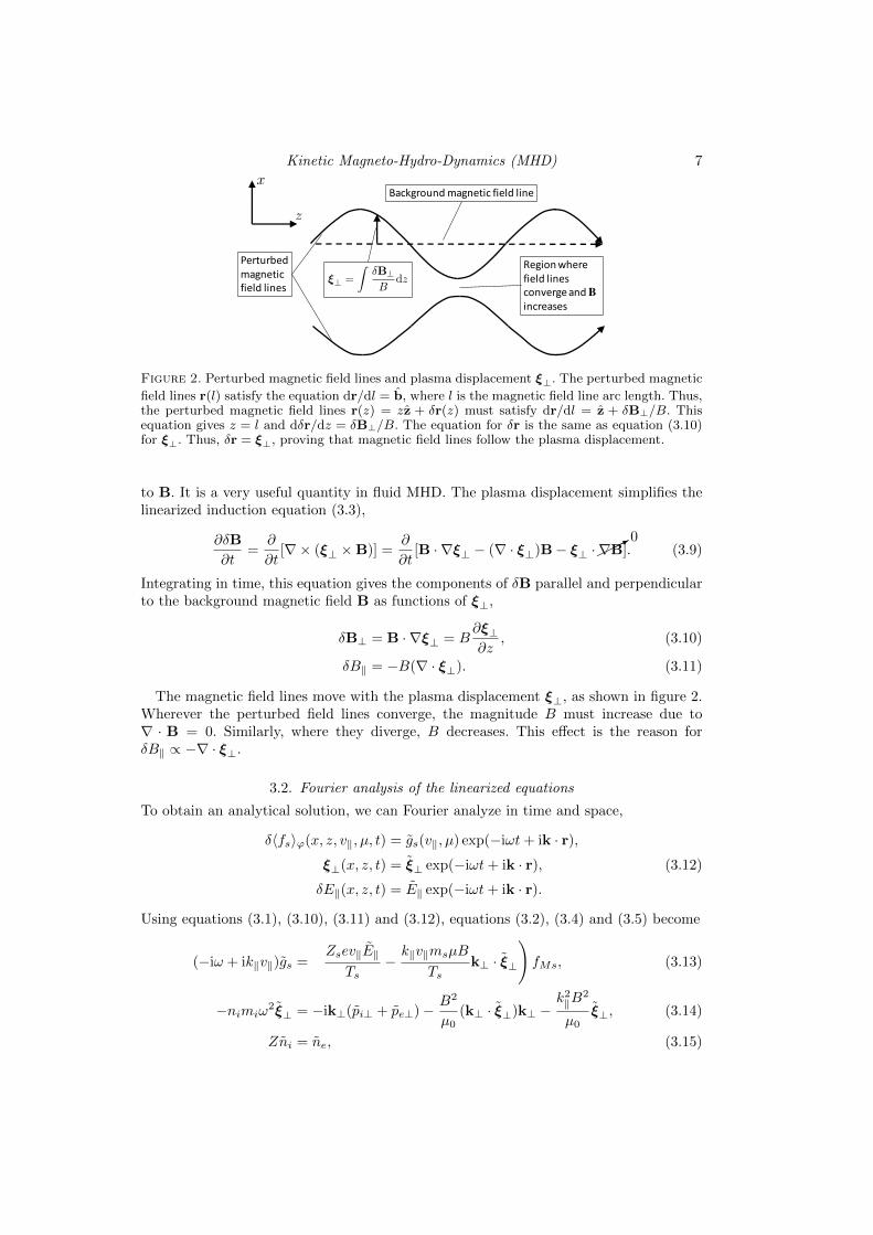
The vector ξ⊥ indicates how far the plasma has moved in the direction perpendicular
Kinetic Magneto-Hydro-Dynamics (MHD) 7
? =
ZB?B
dz
Backgroundmagneticfieldline
Perturbedmagneticfieldlines
RegionwherefieldlinesconvergeandBincreases
z
x
Figure 2. Perturbed magnetic field lines and plasma displacement ξ⊥. The perturbed magnetic
field lines r(l) satisfy the equation dr/dl = b, where l is the magnetic field line arc length. Thus,the perturbed magnetic field lines r(z) = zz + δr(z) must satisfy dr/dl = z + δB⊥/B. Thisequation gives z = l and dδr/dz = δB⊥/B. The equation for δr is the same as equation (3.10)for ξ⊥. Thus, δr = ξ⊥, proving that magnetic field lines follow the plasma displacement.
to B. It is a very useful quantity in fluid MHD. The plasma displacement simplifies thelinearized induction equation (3.3),
∂δB
∂t=
∂
∂t[∇× (ξ⊥ ×B)] =
∂
∂t[B · ∇ξ⊥ − (∇ · ξ⊥)B− ξ⊥ ·*
0∇B]. (3.9)
Integrating in time, this equation gives the components of δB parallel and perpendicularto the background magnetic field B as functions of ξ⊥,
δB⊥ = B · ∇ξ⊥ = B∂ξ⊥∂z
, (3.10)
δB‖ = −B(∇ · ξ⊥). (3.11)
The magnetic field lines move with the plasma displacement ξ⊥, as shown in figure 2.Wherever the perturbed field lines converge, the magnitude B must increase due to∇ · B = 0. Similarly, where they diverge, B decreases. This effect is the reason forδB‖ ∝ −∇ · ξ⊥.
3.2. Fourier analysis of the linearized equations
To obtain an analytical solution, we can Fourier analyze in time and space,
δ〈fs〉ϕ(x, z, v‖, µ, t) = gs(v‖, µ) exp(−iωt+ ik · r),
ξ⊥(x, z, t) = ξ⊥ exp(−iωt+ ik · r), (3.12)
δE‖(x, z, t) = E‖ exp(−iωt+ ik · r).
Using equations (3.1), (3.10), (3.11) and (3.12), equations (3.2), (3.4) and (3.5) become
(−iω + ik‖v‖)gs =
(Zsev‖E‖
Ts− k‖v‖msµB
Tsk⊥ · ξ⊥
)fMs, (3.13)
−nimiω2ξ⊥ = −ik⊥(pi⊥ + pe⊥)− B2
µ0(k⊥ · ξ⊥)k⊥ −
k2‖B
2
µ0ξ⊥, (3.14)
Zni = ne, (3.15)
8 Felix I. Parra
where
ns =
∫2πBgs dv‖ dµ− i(k⊥ · ξ⊥)ns, (3.16)
ps⊥ =
∫2πB2gsmsµdv‖ dµ− 2i(k⊥ · ξ⊥)nsTs. (3.17)
To find non-trivial solutions, we first solve for gs using equation (3.13),
gs = − ik‖v‖k‖v‖ − ω
(ZseE‖k‖Ts
− msµB
Tsk⊥ · ξ⊥
)fMs. (3.18)
The distribution function gs is then used to calculate the ion and electron densities,and the ion and electron perpendicular pressures. The part of the integral over µ isstraightforward. For the integral over v‖, we change to the variable u = (k‖/|k‖|)(v‖/vts),where vts =
√2Ts/ms, and we recall that we need to use the Landau contour for the
integral over u (Schekochihin 2015). Using the plasma dispersion function
Z(ζs) =1√π
∫
CL
exp(−u2)
u− ζsdu (3.19)
and
1√π
∫
CL
u exp(−u2)
u− ζsdu = 1 + ζsZ(ζs), (3.20)
the perturbed densities and pressures become
ns = −i[1 + ζsZ(ζs)]ZseE‖k‖Ts
ns + iζsZ(ζs)(k⊥ · ξ⊥)ns, (3.21)
ps⊥ = −i[1 + ζsZ(ζs)]ZseE‖k‖Ts
nsTs + 2iζsZ(ζs)(k⊥ · ξ⊥)nsTs. (3.22)
Using (3.21) and (3.22) in (3.14) and (3.15), we find
(k2‖B
2
µ0neTe− miω
2
ZTe
)ξ⊥ + [ζiZ(ζi)− ζeZ(ζe)]
eE‖k‖Te
k⊥
+
[B2
µ0neTe− 2TiZTe
ζiZ(ζi)− 2ζeZ(ζe)
](k⊥ · ξ⊥)k⊥ = 0, (3.23)
ZTeTi
[1 + ζiZ(ζi)] + 1 + ζeZ(ζe)
eE‖k‖Te
+ [ζeZ(ζe)− ζiZ(ζi)]k⊥ · ξ⊥ = 0. (3.24)
The solutions to equations (3.23) and (3.24) become clearer if we project the vector
equation (3.23) onto the directions k⊥ × b and k⊥. Then, we find
W11 0 00 W22 W23
0 −W23 W33
ξ⊥ · (k⊥ × b)
k⊥ · ξ⊥eE‖/k‖Te
=
000
, (3.25)
Kinetic Magneto-Hydro-Dynamics (MHD) 9
where
W11 =B2
µ0neTe− miω
2
ZTek2‖, (3.26)
W22 =B2
µ0neTe
k2
k2⊥− miω
2
ZTek2⊥− 2TiZTe
ζiZ(ζi)− 2ζeZ(ζe), (3.27)
W23 = ζiZ(ζi)− ζeZ(ζe), (3.28)
W33 =ZTeTi
[1 + ζiZ(ζi)] + 1 + ζeZ(ζe). (3.29)
We proceed to find solutions to (3.25).
3.3. Shear Alfven waves
One obvious solution to (3.25) is k⊥ ·ξ⊥ = 0 = E‖. Then, the wave has to satisfy W11 = 0,giving
ω = k‖vA, (3.30)
where
vA =
√B2
µ0nimi(3.31)
is the Alfven speed. This solution is known as the shear Alfven wave. One of its strikingfeatures is that it is not damped. The reason for this lack of damping is that the Alfvenwave does not induce a parallel electric field or a perturbation to the magnitude of themagnetic field, B‖ = −iB(k⊥ · ξ⊥) = 0.
3.4. Compressional modes
The other solutions to equation (3.25) satisfy ξ⊥ · (k⊥ × b) = 0. The equations for thesemode are (
W22 W23
−W23 W33
)(k⊥ · ξ⊥eE‖/k‖Te
)=
(00
). (3.32)
Since the matrix must be singular, the frequency is determined by setting the determinantof the matrix to zero, that is,
W22W33 +W 223 = 0. (3.33)
The least damped solutions of equation (3.33) are known with various names. Here wecall them non-propagating modes and magnetosonic waves.
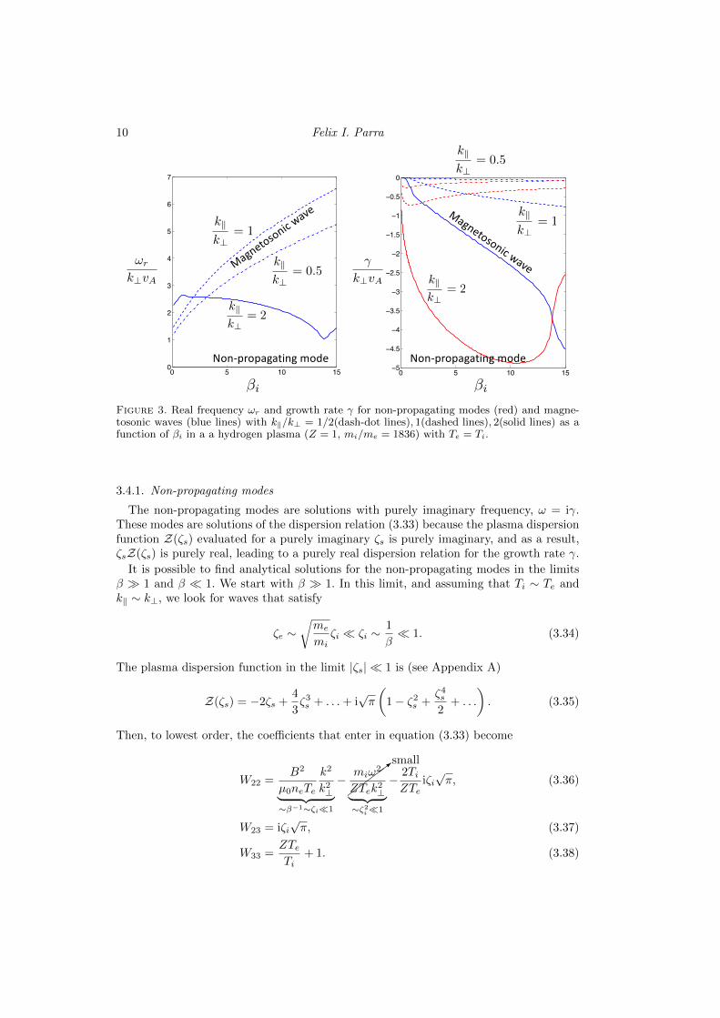
We can solve the dispersion relation (3.33) numerically. In figure 3, for a hydrogenplasma (Z = 1, mi/me = 1836) with Te = Ti, we plot the complex frequency ω = ωr +iγof non-propagating modes and magnetosonic waves as a function of βi = 2µ0niTi/B
2
for several values of k‖/k⊥. The real frequency of the non-propagating mode is zero,that is, the fluctuations due to this mode damp without oscillating. These modes arenon-propagating because their phase velocity ωr/k is zero. The magnetosonic wave is adamped wave that is the equivalent of a sound wave in hydrodynamics. In kinetic MHD,sound waves are due to compressions and expansions of both the plasma and the magneticfield. Note that the damping rate of the non-propagating modes and the magnetosonicwaves increases with the size of k‖.
We proceed to obtain analytical solutions for both modes in some interesting limits.
10 Felix I. Parra
0 5 10 150
1
2
3
4
5
6
7
0 5 10 15−5
−4.5
−4
−3.5
−3
−2.5
−2
−1.5
−1
−0.5
0
0 5 10 150
1
2
3
4
5
6
7
0 5 10 15−5
−4.5
−4
−3.5
−3
−2.5
−2
−1.5
−1
−0.5
0
!r
k?vA<latexit sha1_base64="buFwXgLsQ/8yry7FJdkZVRUVlpg=">AAACBXicbZDLSsNAFIYn9VbrLepSF4NFcFUSEXRZdeOygr1AE8JketIOnSTDzKRQQjdufBU3LhRx6zu4822ctllo6w8DH/85hzPnDwVnSjvOt1VaWV1b3yhvVra2d3b37P2DlkozSaFJU57KTkgUcJZAUzPNoSMkkDjk0A6Ht9N6ewRSsTR50GMBfkz6CYsYJdpYgX3sRZLQ3Etj6JNATvJh4AmQAo+C60lgV52aMxNeBreAKirUCOwvr5fSLIZEU06U6rqO0H5OpGaUw6TiZQoEoUPSh67BhMSg/Hx2xQSfGqeHo1Sal2g8c39P5CRWahyHpjMmeqAWa1Pzv1o309GVn7NEZBoSOl8UZRzrFE8jwT0mgWo+NkCoZOavmA6IiUWb4ComBHfx5GVonddcw/cX1fpNEUcZHaETdIZcdInq6A41UBNR9Iie0St6s56sF+vd+pi3lqxi5hD9kfX5AyGBmPQ=</latexit><latexit sha1_base64="buFwXgLsQ/8yry7FJdkZVRUVlpg=">AAACBXicbZDLSsNAFIYn9VbrLepSF4NFcFUSEXRZdeOygr1AE8JketIOnSTDzKRQQjdufBU3LhRx6zu4822ctllo6w8DH/85hzPnDwVnSjvOt1VaWV1b3yhvVra2d3b37P2DlkozSaFJU57KTkgUcJZAUzPNoSMkkDjk0A6Ht9N6ewRSsTR50GMBfkz6CYsYJdpYgX3sRZLQ3Etj6JNATvJh4AmQAo+C60lgV52aMxNeBreAKirUCOwvr5fSLIZEU06U6rqO0H5OpGaUw6TiZQoEoUPSh67BhMSg/Hx2xQSfGqeHo1Sal2g8c39P5CRWahyHpjMmeqAWa1Pzv1o309GVn7NEZBoSOl8UZRzrFE8jwT0mgWo+NkCoZOavmA6IiUWb4ComBHfx5GVonddcw/cX1fpNEUcZHaETdIZcdInq6A41UBNR9Iie0St6s56sF+vd+pi3lqxi5hD9kfX5AyGBmPQ=</latexit><latexit sha1_base64="buFwXgLsQ/8yry7FJdkZVRUVlpg=">AAACBXicbZDLSsNAFIYn9VbrLepSF4NFcFUSEXRZdeOygr1AE8JketIOnSTDzKRQQjdufBU3LhRx6zu4822ctllo6w8DH/85hzPnDwVnSjvOt1VaWV1b3yhvVra2d3b37P2DlkozSaFJU57KTkgUcJZAUzPNoSMkkDjk0A6Ht9N6ewRSsTR50GMBfkz6CYsYJdpYgX3sRZLQ3Etj6JNATvJh4AmQAo+C60lgV52aMxNeBreAKirUCOwvr5fSLIZEU06U6rqO0H5OpGaUw6TiZQoEoUPSh67BhMSg/Hx2xQSfGqeHo1Sal2g8c39P5CRWahyHpjMmeqAWa1Pzv1o309GVn7NEZBoSOl8UZRzrFE8jwT0mgWo+NkCoZOavmA6IiUWb4ComBHfx5GVonddcw/cX1fpNEUcZHaETdIZcdInq6A41UBNR9Iie0St6s56sF+vd+pi3lqxi5hD9kfX5AyGBmPQ=</latexit><latexit sha1_base64="buFwXgLsQ/8yry7FJdkZVRUVlpg=">AAACBXicbZDLSsNAFIYn9VbrLepSF4NFcFUSEXRZdeOygr1AE8JketIOnSTDzKRQQjdufBU3LhRx6zu4822ctllo6w8DH/85hzPnDwVnSjvOt1VaWV1b3yhvVra2d3b37P2DlkozSaFJU57KTkgUcJZAUzPNoSMkkDjk0A6Ht9N6ewRSsTR50GMBfkz6CYsYJdpYgX3sRZLQ3Etj6JNATvJh4AmQAo+C60lgV52aMxNeBreAKirUCOwvr5fSLIZEU06U6rqO0H5OpGaUw6TiZQoEoUPSh67BhMSg/Hx2xQSfGqeHo1Sal2g8c39P5CRWahyHpjMmeqAWa1Pzv1o309GVn7NEZBoSOl8UZRzrFE8jwT0mgWo+NkCoZOavmA6IiUWb4ComBHfx5GVonddcw/cX1fpNEUcZHaETdIZcdInq6A41UBNR9Iie0St6s56sF+vd+pi3lqxi5hD9kfX5AyGBmPQ=</latexit>
k?vA<latexit sha1_base64="rOK7DogCKUG+hIGsU59kMt3pk04=">AAACA3icbZDLSgMxFIYz9VbrbdSdboJFcFVmRNBl1Y3LCvYCnWHIpJk2NMmEJFMoQ8GNr+LGhSJufQl3vo1pOwtt/SHw8Z9zODl/LBnVxvO+ndLK6tr6RnmzsrW9s7vn7h+0dJopTJo4ZanqxEgTRgVpGmoY6UhFEI8ZacfD22m9PSJK01Q8mLEkIUd9QROKkbFW5B4FiUI4D/qIczTJh1EgiZJwFF1PIrfq1byZ4DL4BVRBoUbkfgW9FGecCIMZ0rrre9KEOVKGYkYmlSDTRCI8RH3StSgQJzrMZzdM4Kl1ejBJlX3CwJn7eyJHXOsxj20nR2agF2tT879aNzPJVZhTITNDBJ4vSjIGTQqngcAeVQQbNraAsKL2rxAPkA3F2NgqNgR/8eRlaJ3XfMv3F9X6TRFHGRyDE3AGfHAJ6uAONEATYPAInsEreHOenBfn3fmYt5acYuYQ/JHz+QN7HJgJ</latexit><latexit sha1_base64="rOK7DogCKUG+hIGsU59kMt3pk04=">AAACA3icbZDLSgMxFIYz9VbrbdSdboJFcFVmRNBl1Y3LCvYCnWHIpJk2NMmEJFMoQ8GNr+LGhSJufQl3vo1pOwtt/SHw8Z9zODl/LBnVxvO+ndLK6tr6RnmzsrW9s7vn7h+0dJopTJo4ZanqxEgTRgVpGmoY6UhFEI8ZacfD22m9PSJK01Q8mLEkIUd9QROKkbFW5B4FiUI4D/qIczTJh1EgiZJwFF1PIrfq1byZ4DL4BVRBoUbkfgW9FGecCIMZ0rrre9KEOVKGYkYmlSDTRCI8RH3StSgQJzrMZzdM4Kl1ejBJlX3CwJn7eyJHXOsxj20nR2agF2tT879aNzPJVZhTITNDBJ4vSjIGTQqngcAeVQQbNraAsKL2rxAPkA3F2NgqNgR/8eRlaJ3XfMv3F9X6TRFHGRyDE3AGfHAJ6uAONEATYPAInsEreHOenBfn3fmYt5acYuYQ/JHz+QN7HJgJ</latexit><latexit sha1_base64="rOK7DogCKUG+hIGsU59kMt3pk04=">AAACA3icbZDLSgMxFIYz9VbrbdSdboJFcFVmRNBl1Y3LCvYCnWHIpJk2NMmEJFMoQ8GNr+LGhSJufQl3vo1pOwtt/SHw8Z9zODl/LBnVxvO+ndLK6tr6RnmzsrW9s7vn7h+0dJopTJo4ZanqxEgTRgVpGmoY6UhFEI8ZacfD22m9PSJK01Q8mLEkIUd9QROKkbFW5B4FiUI4D/qIczTJh1EgiZJwFF1PIrfq1byZ4DL4BVRBoUbkfgW9FGecCIMZ0rrre9KEOVKGYkYmlSDTRCI8RH3StSgQJzrMZzdM4Kl1ejBJlX3CwJn7eyJHXOsxj20nR2agF2tT879aNzPJVZhTITNDBJ4vSjIGTQqngcAeVQQbNraAsKL2rxAPkA3F2NgqNgR/8eRlaJ3XfMv3F9X6TRFHGRyDE3AGfHAJ6uAONEATYPAInsEreHOenBfn3fmYt5acYuYQ/JHz+QN7HJgJ</latexit><latexit sha1_base64="rOK7DogCKUG+hIGsU59kMt3pk04=">AAACA3icbZDLSgMxFIYz9VbrbdSdboJFcFVmRNBl1Y3LCvYCnWHIpJk2NMmEJFMoQ8GNr+LGhSJufQl3vo1pOwtt/SHw8Z9zODl/LBnVxvO+ndLK6tr6RnmzsrW9s7vn7h+0dJopTJo4ZanqxEgTRgVpGmoY6UhFEI8ZacfD22m9PSJK01Q8mLEkIUd9QROKkbFW5B4FiUI4D/qIczTJh1EgiZJwFF1PIrfq1byZ4DL4BVRBoUbkfgW9FGecCIMZ0rrre9KEOVKGYkYmlSDTRCI8RH3StSgQJzrMZzdM4Kl1ejBJlX3CwJn7eyJHXOsxj20nR2agF2tT879aNzPJVZhTITNDBJ4vSjIGTQqngcAeVQQbNraAsKL2rxAPkA3F2NgqNgR/8eRlaJ3XfMv3F9X6TRFHGRyDE3AGfHAJ6uAONEATYPAInsEreHOenBfn3fmYt5acYuYQ/JHz+QN7HJgJ</latexit>
i<latexit sha1_base64="tvCXPjL22/u9V+lvg65saor4LyY=">AAAB7nicbZDLSgNBEEVrfMb4irp00xgEV2FGBF0G3biMYB6QDKGnU5M06XnQXSOEIR/hxoUibv0ed/6NnWQWmnih4XCriq66QaqkIdf9dtbWNza3tks75d29/YPDytFxyySZFtgUiUp0J+AGlYyxSZIUdlKNPAoUtoPx3azefkJtZBI/0iRFP+LDWIZScLJWuxcg8b7sV6puzZ2LrYJXQBUKNfqVr94gEVmEMQnFjel6bkp+zjVJoXBa7mUGUy7GfIhdizGP0Pj5fN0pO7fOgIWJti8mNnd/T+Q8MmYSBbYz4jQyy7WZ+V+tm1F44+cyTjPCWCw+CjPFKGGz29lAahSkJha40NLuysSIay7IJlS2IXjLJ69C67LmWX64qtZvizhKcApncAEeXEMd7qEBTRAwhmd4hTcndV6cd+dj0brmFDMn8EfO5w9BP4+A</latexit><latexit sha1_base64="tvCXPjL22/u9V+lvg65saor4LyY=">AAAB7nicbZDLSgNBEEVrfMb4irp00xgEV2FGBF0G3biMYB6QDKGnU5M06XnQXSOEIR/hxoUibv0ed/6NnWQWmnih4XCriq66QaqkIdf9dtbWNza3tks75d29/YPDytFxyySZFtgUiUp0J+AGlYyxSZIUdlKNPAoUtoPx3azefkJtZBI/0iRFP+LDWIZScLJWuxcg8b7sV6puzZ2LrYJXQBUKNfqVr94gEVmEMQnFjel6bkp+zjVJoXBa7mUGUy7GfIhdizGP0Pj5fN0pO7fOgIWJti8mNnd/T+Q8MmYSBbYz4jQyy7WZ+V+tm1F44+cyTjPCWCw+CjPFKGGz29lAahSkJha40NLuysSIay7IJlS2IXjLJ69C67LmWX64qtZvizhKcApncAEeXEMd7qEBTRAwhmd4hTcndV6cd+dj0brmFDMn8EfO5w9BP4+A</latexit><latexit sha1_base64="tvCXPjL22/u9V+lvg65saor4LyY=">AAAB7nicbZDLSgNBEEVrfMb4irp00xgEV2FGBF0G3biMYB6QDKGnU5M06XnQXSOEIR/hxoUibv0ed/6NnWQWmnih4XCriq66QaqkIdf9dtbWNza3tks75d29/YPDytFxyySZFtgUiUp0J+AGlYyxSZIUdlKNPAoUtoPx3azefkJtZBI/0iRFP+LDWIZScLJWuxcg8b7sV6puzZ2LrYJXQBUKNfqVr94gEVmEMQnFjel6bkp+zjVJoXBa7mUGUy7GfIhdizGP0Pj5fN0pO7fOgIWJti8mNnd/T+Q8MmYSBbYz4jQyy7WZ+V+tm1F44+cyTjPCWCw+CjPFKGGz29lAahSkJha40NLuysSIay7IJlS2IXjLJ69C67LmWX64qtZvizhKcApncAEeXEMd7qEBTRAwhmd4hTcndV6cd+dj0brmFDMn8EfO5w9BP4+A</latexit><latexit sha1_base64="tvCXPjL22/u9V+lvg65saor4LyY=">AAAB7nicbZDLSgNBEEVrfMb4irp00xgEV2FGBF0G3biMYB6QDKGnU5M06XnQXSOEIR/hxoUibv0ed/6NnWQWmnih4XCriq66QaqkIdf9dtbWNza3tks75d29/YPDytFxyySZFtgUiUp0J+AGlYyxSZIUdlKNPAoUtoPx3azefkJtZBI/0iRFP+LDWIZScLJWuxcg8b7sV6puzZ2LrYJXQBUKNfqVr94gEVmEMQnFjel6bkp+zjVJoXBa7mUGUy7GfIhdizGP0Pj5fN0pO7fOgIWJti8mNnd/T+Q8MmYSBbYz4jQyy7WZ+V+tm1F44+cyTjPCWCw+CjPFKGGz29lAahSkJha40NLuysSIay7IJlS2IXjLJ69C67LmWX64qtZvizhKcApncAEeXEMd7qEBTRAwhmd4hTcndV6cd+dj0brmFDMn8EfO5w9BP4+A</latexit>
i<latexit sha1_base64="tvCXPjL22/u9V+lvg65saor4LyY=">AAAB7nicbZDLSgNBEEVrfMb4irp00xgEV2FGBF0G3biMYB6QDKGnU5M06XnQXSOEIR/hxoUibv0ed/6NnWQWmnih4XCriq66QaqkIdf9dtbWNza3tks75d29/YPDytFxyySZFtgUiUp0J+AGlYyxSZIUdlKNPAoUtoPx3azefkJtZBI/0iRFP+LDWIZScLJWuxcg8b7sV6puzZ2LrYJXQBUKNfqVr94gEVmEMQnFjel6bkp+zjVJoXBa7mUGUy7GfIhdizGP0Pj5fN0pO7fOgIWJti8mNnd/T+Q8MmYSBbYz4jQyy7WZ+V+tm1F44+cyTjPCWCw+CjPFKGGz29lAahSkJha40NLuysSIay7IJlS2IXjLJ69C67LmWX64qtZvizhKcApncAEeXEMd7qEBTRAwhmd4hTcndV6cd+dj0brmFDMn8EfO5w9BP4+A</latexit><latexit sha1_base64="tvCXPjL22/u9V+lvg65saor4LyY=">AAAB7nicbZDLSgNBEEVrfMb4irp00xgEV2FGBF0G3biMYB6QDKGnU5M06XnQXSOEIR/hxoUibv0ed/6NnWQWmnih4XCriq66QaqkIdf9dtbWNza3tks75d29/YPDytFxyySZFtgUiUp0J+AGlYyxSZIUdlKNPAoUtoPx3azefkJtZBI/0iRFP+LDWIZScLJWuxcg8b7sV6puzZ2LrYJXQBUKNfqVr94gEVmEMQnFjel6bkp+zjVJoXBa7mUGUy7GfIhdizGP0Pj5fN0pO7fOgIWJti8mNnd/T+Q8MmYSBbYz4jQyy7WZ+V+tm1F44+cyTjPCWCw+CjPFKGGz29lAahSkJha40NLuysSIay7IJlS2IXjLJ69C67LmWX64qtZvizhKcApncAEeXEMd7qEBTRAwhmd4hTcndV6cd+dj0brmFDMn8EfO5w9BP4+A</latexit><latexit sha1_base64="tvCXPjL22/u9V+lvg65saor4LyY=">AAAB7nicbZDLSgNBEEVrfMb4irp00xgEV2FGBF0G3biMYB6QDKGnU5M06XnQXSOEIR/hxoUibv0ed/6NnWQWmnih4XCriq66QaqkIdf9dtbWNza3tks75d29/YPDytFxyySZFtgUiUp0J+AGlYyxSZIUdlKNPAoUtoPx3azefkJtZBI/0iRFP+LDWIZScLJWuxcg8b7sV6puzZ2LrYJXQBUKNfqVr94gEVmEMQnFjel6bkp+zjVJoXBa7mUGUy7GfIhdizGP0Pj5fN0pO7fOgIWJti8mNnd/T+Q8MmYSBbYz4jQyy7WZ+V+tm1F44+cyTjPCWCw+CjPFKGGz29lAahSkJha40NLuysSIay7IJlS2IXjLJ69C67LmWX64qtZvizhKcApncAEeXEMd7qEBTRAwhmd4hTcndV6cd+dj0brmFDMn8EfO5w9BP4+A</latexit><latexit sha1_base64="tvCXPjL22/u9V+lvg65saor4LyY=">AAAB7nicbZDLSgNBEEVrfMb4irp00xgEV2FGBF0G3biMYB6QDKGnU5M06XnQXSOEIR/hxoUibv0ed/6NnWQWmnih4XCriq66QaqkIdf9dtbWNza3tks75d29/YPDytFxyySZFtgUiUp0J+AGlYyxSZIUdlKNPAoUtoPx3azefkJtZBI/0iRFP+LDWIZScLJWuxcg8b7sV6puzZ2LrYJXQBUKNfqVr94gEVmEMQnFjel6bkp+zjVJoXBa7mUGUy7GfIhdizGP0Pj5fN0pO7fOgIWJti8mNnd/T+Q8MmYSBbYz4jQyy7WZ+V+tm1F44+cyTjPCWCw+CjPFKGGz29lAahSkJha40NLuysSIay7IJlS2IXjLJ69C67LmWX64qtZvizhKcApncAEeXEMd7qEBTRAwhmd4hTcndV6cd+dj0brmFDMn8EfO5w9BP4+A</latexit>
Magnetosonic wave
Non-propagating mode
kkk?
= 2<latexit sha1_base64="(null)">(null)</latexit><latexit sha1_base64="(null)">(null)</latexit><latexit sha1_base64="(null)">(null)</latexit><latexit sha1_base64="(null)">(null)</latexit>
kkk?
= 1<latexit sha1_base64="(null)">(null)</latexit><latexit sha1_base64="(null)">(null)</latexit><latexit sha1_base64="(null)">(null)</latexit><latexit sha1_base64="(null)">(null)</latexit>
kkk?
= 0.5<latexit sha1_base64="(null)">(null)</latexit><latexit sha1_base64="(null)">(null)</latexit><latexit sha1_base64="(null)">(null)</latexit><latexit sha1_base64="(null)">(null)</latexit>
Non-propagating mode
Magnetosonic wavekkk?
= 2<latexit sha1_base64="(null)">(null)</latexit><latexit sha1_base64="(null)">(null)</latexit><latexit sha1_base64="(null)">(null)</latexit><latexit sha1_base64="(null)">(null)</latexit>
kkk?
= 1<latexit sha1_base64="(null)">(null)</latexit><latexit sha1_base64="(null)">(null)</latexit><latexit sha1_base64="(null)">(null)</latexit><latexit sha1_base64="(null)">(null)</latexit>
kkk?
= 0.5<latexit sha1_base64="(null)">(null)</latexit><latexit sha1_base64="(null)">(null)</latexit><latexit sha1_base64="(null)">(null)</latexit><latexit sha1_base64="(null)">(null)</latexit>
Figure 3. Real frequency ωr and growth rate γ for non-propagating modes (red) and magne-tosonic waves (blue lines) with k‖/k⊥ = 1/2(dash-dot lines), 1(dashed lines), 2(solid lines) as afunction of βi in a a hydrogen plasma (Z = 1, mi/me = 1836) with Te = Ti.
3.4.1. Non-propagating modes
The non-propagating modes are solutions with purely imaginary frequency, ω = iγ.These modes are solutions of the dispersion relation (3.33) because the plasma dispersionfunction Z(ζs) evaluated for a purely imaginary ζs is purely imaginary, and as a result,ζsZ(ζs) is purely real, leading to a purely real dispersion relation for the growth rate γ.
It is possible to find analytical solutions for the non-propagating modes in the limitsβ 1 and β 1. We start with β 1. In this limit, and assuming that Ti ∼ Te andk‖ ∼ k⊥, we look for waves that satisfy
ζe ∼√me
miζi ζi ∼
1
β 1. (3.34)
The plasma dispersion function in the limit |ζs| 1 is (see Appendix A)
Z(ζs) = −2ζs +4
3ζ3s + . . .+ i
√π
(1− ζ2
s +ζ4s
2+ . . .
). (3.35)
Then, to lowest order, the coefficients that enter in equation (3.33) become
W22 =B2
µ0neTe
k2
k2⊥︸ ︷︷ ︸
∼β−1∼ζi1
−>
smallmiω
2
ZTek2⊥︸ ︷︷ ︸
∼ζ2i1
− 2TiZTe
iζi√π, (3.36)
W23 = iζi√π, (3.37)
W33 =ZTeTi
+ 1. (3.38)
Kinetic Magneto-Hydro-Dynamics (MHD) 11
With these results, equation (3.33) becomes to lowest order W22 ' 0, that is,
ω ' − i√π
B2
2µ0niTi
k2
k2⊥|k‖|vti. (3.39)
This result satisfies the condition ζi ∼ β−1 1 that we assumed at the start of thecalculation. The damping arises from the magnetic bottling force, represented in thiscalculation by the ion perpendicular pressure, given by equation (3.22). The perturbations
in the magnetic field strength, δB‖, cause a magnetic bottling force −miµb · ∇B thatacts as a parallel electric field, and like the parallel electric field in electrostatic waves,it can lead to Landau damping. When it is caused by the magnetic bottling force, it iscalled Barnes damping.
For β 1, and assuming that Ti ∼ Te and k‖ ∼ k⊥, we search for solutions of the formω = iγ, where γ is a negative number that satisfies |γ|/|k‖|vti 1. Then, ζi = ω/|k‖|vtiis a very large imaginary number and the largest contribution to the plasma dispersionfunction is the exponentially large piece
Z(ζi) ' 2i√π exp(−ζ2
i ) = 2i√π exp
(γ2
k2‖v
2ti
). (3.40)
The electron contribution is smaller because ζe ∼ ζi√me/mi ζi. Using these results,
the coefficients that enter in equation (3.33) can be approximated by
W22 =B2
µ0neTe
k2
k2⊥
+>
smallmiγ
2
ZTek2⊥︸ ︷︷ ︸
∼ γ2
k2‖v2ti
exp
(γ2
k2‖v2ti
)+
4√πTi
ZTe
γ
|k‖|vtiexp
(γ2
k2‖v
2ti
), (3.41)
W23 =TiZTe
W33 = − 2√πγ
|k‖|vtiexp
(γ2
k2‖v
2ti
). (3.42)
Then, equation (3.33) becomes W22 + (Ti/ZTe)W23 ' 0,
|γ||k‖|vti
exp
(γ2
k2‖v
2ti
)=
1√π
B2
2µ0niTi
k2
k2⊥. (3.43)
Solving this equation, we find
ω = iγ ' −i
√√√√ln
(k2
k2⊥√πβi
1√ln(k2/k2
⊥√πβi)
)|k‖|vti. (3.44)
Thus, our assumption |γ|/|k‖|vti 1 is satisfied because |γ|/|k‖|vti ∼√
ln(1/β).
3.4.2. Magnetosonic waves
To obtain an analytical solution for the magnetosonic waves, we consider the limit√mi
me
√βk‖k⊥ 1 . 1
β. (3.45)
Note that this limit could be achieved in systems with either β 1, k‖/k⊥ 1 or bothat the same time.
12 Felix I. Parra
The magnetosonic waves will have a frequency ω ∼ k⊥vA. Thus, assuming Ti ∼ Te,
1 ζe ∼√me
mi
1√β
k⊥k‖∼√me
miζi ζi ∼
1√β
k⊥k‖. (3.46)
We will find that the imaginary part of ω is much smaller than the real part. Takingthis into account and using |ζs| 1, the plasma dispersion function becomes (see Ap-pendix B)
Z(ζs) = − 1
ζs− 1
2ζ3s
− 3
4ζ5s
+ . . .+ i√π exp(−ζ2
s ). (3.47)
Using this expansion, the coefficients that enter in equation (3.33) become
W22 'B2
µ0neTe
k2
k2⊥
+2TiZTe
+ 2− miω2
ZTek2⊥︸ ︷︷ ︸
∼β−1&1
+1
ζ2e
− 2i√πζe exp(−ζ2
e ), (3.48)
W23 ' −W33 '1
2ζ2e
− i√πζe exp(−ζ2
e ). (3.49)
With these results, equation (3.33) becomes to lowest order W22 −W23 ' 0,
B2
µ0neTe
k2
k2⊥︸ ︷︷ ︸
∼β−1&1
+2TiZTe
+ 2− miω2
ZTek2⊥︸ ︷︷ ︸
∼β−1&1
+1
2ζ2e
− i√πζe exp(−ζ2
e ) = 0 (3.50)
This equation can be solved order by order in ζ−1e 1. The frequency is of the form
ω ' ω(0) + ω(1) + iγ, where ω(1)/ω(0) ∼ ζ−2e 1 and γ/ω(0) ∼ exp(−ζ2
e ) 1. Tolowest order, we find
(ω(0))2 = k2v2A +
2k2⊥(Ti + ZTe)
mi= k2v2
A
[1 +
k2⊥k2
(βi + βe)
], (3.51)
where βe = 2µ0neTe/B2. To next order, neglecting the exponentially small imaginary
piece, we find
ω(1)
ω(0)=
ZTek2⊥
4mi(ω(0))2(ζ(0)e )2
=1
8
k2⊥k
2‖
[k2 + k2⊥(βi + βe)]2
mi
me
β2e
Z︸ ︷︷ ︸∼k2‖k2⊥
mime
β2.k2‖k2⊥
mime
β1
, (3.52)
where ζ(0)e = ω(0)/|k‖|vte. Finally, the imaginary part is given by
γ = −√πZTek
2⊥
2miω(0)ζ(0)e exp(−ζ2
e ) ' −√π
4kvA
√me
mi
k2⊥
k|k‖|√Zβe
× exp
(−βe
4
k2⊥
k2 + k2⊥(βi + βe)︸ ︷︷ ︸
∼β.1
− k2 + k2⊥(βi + βe)
k2‖
me
mi
1
βe︸ ︷︷ ︸
∼ k2⊥k2‖
memi
β−11
). (3.53)
Note that we had to keep the higher order correction to ω given in (3.52) inside theexponential because it contributes a number of order unity to the damping rate.
REFERENCES
Kinetic Magneto-Hydro-Dynamics (MHD) 13
Schekochihin, A.A. 2015 Lecture notes on Kinetic Theory and Magnetohydrodynamics ofPlasmas. http://www-thphys.physics.ox.ac.uk/people/AlexanderSchekochihin/KT/.
14 Felix I. Parra
SC
Figure 4. Landau contour for the integral (A 1).
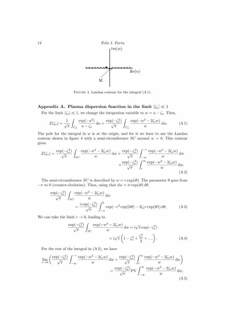
Appendix A. Plasma dispersion function in the limit |ζs| 1
For the limit |ζs| 1, we change the integration variable to w = u− ζs. Then,
Z(ζs) =1√π
∫
CL
exp(−u2)
u− ζsdu =
exp(−ζ2s )√
π
∫
CL
exp(−w2 − 2ζsw)
wdw. (A 1)
The pole for the integral in w is at the origin, and for it we have to use the Landaucontour shown in figure 4 with a semi-circunference SC around w = 0. This contourgives
Z(ζs) =exp(−ζ2
s )√π
∫
SC
exp(−w2 − 2ζsw)
wdw +
exp(−ζ2s )√
π
∫ −r
−∞
exp(−w2 − 2ζsw)
wdw
+exp(−ζ2
s )√π
∫ ∞
r
exp(−w2 − 2ζsw)
wdw.
(A 2)
The semi-circumference SC is described by w = r exp(iθ). The parameter θ goes from−π to 0 (counter-clockwise). Then, using that dw = ir exp(iθ) dθ,
exp(−ζ2s )√
π
∫
SC
exp(−w2 − 2ζsw)
wdw
=i exp(−ζ2
s )√π
∫ 0
−πexp(−r2 exp(2iθ)− 2ζsr exp(iθ)) dθ. (A 3)
We can take the limit r → 0, leading to
exp(−ζ2s )√
π
∫
SC
exp(−w2 − 2ζsw)
wdw = i
√π exp(−ζ2
s )
= i√π
(1− ζ2
s +ζ4s
2+ . . .
). (A 4)
For the rest of the integral in (A 2), we have
limr→0
(exp(−ζ2
s )√π
∫ −r
−∞
exp(−w2 − 2ζsw)
wdw +
exp(−ζ2s )√
π
∫ ∞
r
exp(−w2 − 2ζsw)
wdw
)
=exp(−ζ2
s )√π
PV
∫ ∞
−∞
exp(−w2 − 2ζsw)
wdw,
(A 5)
Kinetic Magneto-Hydro-Dynamics (MHD) 15
where PV indicates that we have to take the Principal Value of the integral. We can use
exp(−w2 − 2ζsw) = exp(−w2)
∞∑
q=0
(−2ζsw)q
q!. (A 6)
Then,
exp(−ζ2s )√
πPV
∫ ∞
−∞
exp(−w2 − 2ζsw)
wdw
= −exp(−ζ2s )√
π
∫ ∞
−∞exp(−w2)
∞∑
p=0
22p+1ζ2p+1s w2p
(2p+ 1)!dw, (A 7)
where the integral over the odd powers of w vanishes due to symmetry. Taking theintegrals over w, we find
exp(−ζ2s )√
πPV
∫ ∞
−∞
exp(−w2 − 2ζsw)
wdw = − exp(−ζ2
s )
∞∑
p=0
22p+1Γ(p+ 1/2)ζ2p+1s
(2p+ 1)!,
(A 8)where Γ(ν) =
∫∞0xν−1 exp(−x) dx is the gamma function.
Combining equations (A 4) and (A 8), we find the approximation (3.35).
Appendix B. Plasma dispersion function in the limit |ζs| 1
Using the Landau contour, we find that the plasma dispersion function for Im(ζs) = 0is
Z(ζs) =1√π
PV
∫ ∞
−∞
exp(−u2)
u− ζsdu+ i
√π exp(−ζ2
s ), (B 1)
where the last term is due to the integral over the semicircle SC. The integral over thereal axis
1√π
PV
∫ ∞
−∞
exp(−u2)
u− ζsdu (B 2)
can be simplified for |ζs| 1. For most of the integration interval, |u| ∼ 1 |ζs|, andthe resonant denominator becomes
1
u− ζs= − 1
ζs
1
1− u/ζs' − 1
ζs
Q∑
q=0
uq
ζqs, (B 3)
leading to the simplified expression
1√π
PV
∫ ∞
−∞
exp(−u2)
u− ζsdu ' − 1
ζs√π
∫ ∞
−∞exp(−u2)
P∑
p=0
u2p
ζ2ps
du, (B 4)
where the integrals that included odd powers of u have vanished due to symmetry. Inte-grating in u, we find
1√π
PV
∫ ∞
−∞
exp(−u2)
u− ζsdu ' − 1
ζs√π
P∑
p=0
Γ(p+ 1/2)
ζ2ps
. (B 5)
Note that the series is an asymptotic expansion (i.e. it diverges for P → ∞) and henceonly a few terms must be kept. Combining the result in equation (B 5) with equation(B 1), we find the formula for the plasma dispersion function given in equation (3.47).
16 Felix I. Parra
Even though we have deduced this formula only for Im(ζs) = 0, we expect it to be validfor sufficiently small Im(ζs). We proceed to argue that this is the case.
The most striking feature of the expansion in equation (3.47) is that we keep theexponentially small term i
√π exp(−ζ2
s ) even though we have neglected terms that aremuch larger (of order 1/|ζs|2P+3). The apparently incongruous decision of keeping theexponentially small term i
√π exp(−ζ2
s ) is justified in cases in which the imaginary partof ζs is also exponentially small, that is,
|Im(ζs)| ∼ |Re(ζs)|α exp(−[Re(ζs)]2) 1 |Re(ζs)| ' |ζs|, (B 6)
where α is a constant that depends on the problem. When Im(ζs) is exponentially small,the term i
√π exp(−ζ2
s ) is comparable to the other terms in the imaginary part of theplasma dispersion function, Im(Z(ζs)). Using the Landau contour, we write the imaginarypart of Z(ζs) for Im(ζs) 6= 0 as
Im(Z(ζs)) =1√π
∫ ∞
−∞I(u) du+ σ
√πRe(exp(−ζ2
s )), (B 7)
where σ = 0 for Im(ζs) > 0 and σ = 2 for Im(ζs) < 0, and the integrand I(u) is
I(u) =Im(ζs) exp(−u2)
[u− Re(ζs)]2 + [Im(ζs)]2. (B 8)
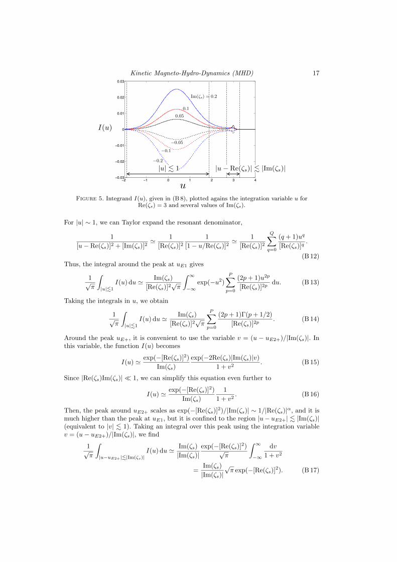
The function I(u) is sketched in figure 5 for Re(ζs) = 3 and various values of Im(ζs).Note that for sufficiently small Im(ζs) there are two clear peaks: one around u = 0 andthe other around u = Re(ζs). We can study both peaks by looking for the minima andmaxima of I(u), located at the points where dI/du = 0. The equation dI/du = 0 givesthe cubic polynomial
u[u− Re(ζs)]2 + [Im(ζs)]
2+ [u− Re(ζs)] = 0. (B 9)
We proceed to find the three roots of this polynomial when |Im(ζs)| 1 |Re(ζs)|.In the region |u| . 1, equation (B 9) is approximately [Re(ζs)]
2u − Re(ζs) = 0, leadingto an extremum at uE1 ' 1/Re(ζs). The value of I(u) at this extremum is I(uE1) 'Im(ζs)/[Re(ζs)]
2, and the function decays exponentially away from it. The other two rootsof the polynomial (B 9) are in the region |u − Re(ζs)| 1. In this limit, equation (B 9)becomes Re(ζs)[u− Re(ζs)]
2 + [Im(ζs)]2+ [u− Re(ζs)] = 0, and the roots are
uE2± ' Re(ζs) +±√
1− 4[Re(ζs)Im(ζs)]2 − 1
2Re(ζs). (B 10)
Note that for |Re(ζs)Im(ζs)| > 1/2 there are no extrema (see the blue curves in figure 5).However, in the limit (B 6), the parameter |Re(ζs)Im(ζs)| is very small, |Re(ζs)Im(ζs)| 1, leading to
uE2+ ' Re(ζs)− Re(ζs)[Im(ζs)]2, uE2− ' Re(ζs)−
1
Re(ζs). (B 11)
The root uE2+ corresponds to the peak, and the value of I(u) in this peak is I(uE2+) 'exp(−[Re(ζs)]
2)/Im(ζs). The root uE2− corresponds to the valley between the two peaks,where the function is I(uE2−) = [Re(ζs)]
2Im(ζs) exp(2− [Re(ζs)]2).
Therefore, in the limit (B 6), both peaks are well separated. The peak at uE1 scales as|Im(ζs)|/[Re(ζs)]
2 ∼ |Re(ζs)|α−2 exp(−[Re(ζs)]2), and it extends to the region |u| ∼ 1.
Kinetic Magneto-Hydro-Dynamics (MHD) 17
−2 −1 0 1 2 3 4−0.03
−0.02
−0.01
0
0.01
0.02
0.03
I(u)
u
Im(s) = 0.2
0.1
0.05
0.05
0.1
0.2
|u| . 1 |u Re(s)| . |Im(s)|
Figure 5. Integrand I(u), given in (B 8), plotted agains the integration variable u forRe(ζs) = 3 and several values of Im(ζs).
For |u| ∼ 1, we can Taylor expand the resonant denominator,
1
[u− Re(ζs)]2 + [Im(ζs)]2' 1
[Re(ζs)]21
[1− u/Re(ζs)]2' 1
[Re(ζs)]2
Q∑
q=0
(q + 1)uq
[Re(ζs)]q.
(B 12)Thus, the integral around the peak at uE1 gives
1√π
∫
|u|.1
I(u) du ' Im(ζs)
[Re(ζs)]2√π
∫ ∞
−∞exp(−u2)
P∑
p=0
(2p+ 1)u2p
[Re(ζs)]2pdu. (B 13)
Taking the integrals in u, we obtain
1√π
∫
|u|.1
I(u) du ' Im(ζs)
[Re(ζs)]2√π
P∑
p=0
(2p+ 1)Γ(p+ 1/2)
[Re(ζs)]2p. (B 14)
Around the peak uE+, it is convenient to use the variable v = (u − uE2+)/|Im(ζs)|. Inthis variable, the function I(u) becomes
I(u) ' exp(−[Re(ζs)]2)
Im(ζs)
exp(−2Re(ζs)|Im(ζs)|v)
1 + v2. (B 15)
Since |Re(ζs)Im(ζs)| 1, we can simplify this equation even further to
I(u) ' exp(−[Re(ζs)]2)
Im(ζs)
1
1 + v2. (B 16)
Then, the peak around uE2+ scales as exp(−[Re(ζs)]2)/|Im(ζs)| ∼ 1/|Re(ζs)|α, and it is
much higher than the peak at uE1, but it is confined to the region |u− uE2+| . |Im(ζs)|(equivalent to |v| . 1). Taking an integral over this peak using the integration variablev = (u− uE2+)/|Im(ζs)|, we find
1√π
∫
|u−uE2+|.|Im(ζs)|I(u) du ' Im(ζs)
|Im(ζs)|exp(−[Re(ζs)]
2)√π
∫ ∞
−∞
dv
1 + v2
=Im(ζs)
|Im(ζs)|√π exp(−[Re(ζs)]
2). (B 17)
18 Felix I. Parra
Adding the two contributions (B 14) and (B 17), equation (B 7) finally becomes
Im(Z(ζs)) 'Im(ζs)
[Re(ζs)]2√π
P∑
p=0
(2p+ 1)Γ(p+ 1/2)
[Re(ζs)]2pdu+
√π exp(−[Re(ζs)]
2). (B 18)
The dependence on the sign of Im(ζs) has disappeared because σ√πRe(exp(−ζ2
s )) +(Im(ζs)/|Im(ζs)|)
√π exp(−[Re(ζs)]
2) ' √π exp(−[Re(ζs)]2).
The first term in equation (B 18) is the imaginary part of the expansion given inequation (B 5) for |Im(ζs)| |Re(ζs)|,
Im
(−
P∑
p=0
Γ(p+ 1/2)
ζ2p+1s√π
)'
P∑
p=0
(2p+ 1)Im(ζs)Γ(p+ 1/2)
[Re(ζs)]2p+2√π
. (B 19)
Thus, equation (B 18) is the correct lowest order approximation to the imaginary com-ponent of Z(ζs) when assumption (B 6) is satisfied, justifying the use of equation (3.47).Note that, in deriving this result, we have used repeatedly the fact that under assump-tion (B 6), |Re(ζs)Im(ζs)| 1. For this reason, the result in equation (3.47) is sometimesreferred to as the |Re(ζs)Im(ζs)| 1 limit even though it is only really valid in the morestringent limit (B 6).