Kai Wang Dan Milkie Ankur Saxena Peter Engerer Thomas...

Rapid Adaptive Optical Recovery of Optimal Resolution overLargeVolumes

Kai Wang1, Dan Milkie2, Ankur Saxena3, Peter Engerer4,5,6, Thomas Misgeld4,5,6, MarianneE. Bronner3, Jeff Mumm7,8, and Eric Betzig1

1Janelia Farm Research Campus, Howard Hughes Medical Institute, Ashburn, Virginia, USA

2Coleman Technologies, Inc., Newtown Square, Pennsylvania, USA

3Division of Biology, California Institute of Technology, Pasadena, California, USA

4Institute of Neuronal Cell Biology, Technische Universität München, Munich, Germany

5Munich Center for Systems Neurology, Munich, Germany

6German Center for Neurodegenerative Diseases, Munich, Germany

7Department of Cellular Biology and Anatomy, Georgia Regents University, Augusta, Georgia,USA

Abstract

Using a de-scanned, laser-induced guide star and direct wavefront sensing, we demonstrate

adaptive correction of complex optical aberrations at high numerical aperture and a 14 ms update

rate. This permits us to compensate for the rapid spatial variation in aberration often encountered

in biological specimens, and recover diffraction-limited imaging over large (> 240 μm)3 volumes.

We applied this to image fine neuronal processes and subcellular dynamics within the zebrafish

brain.

Optical imaging at diffraction-limited resolution in whole living organisms, where cell-cell

interactions play crucial roles, is difficult due to refractive index heterogeneities arising from

different cell morphologies within tissues and sub-cellular domains within cells. While

adaptive optics1 (AO) using a variety of approaches has been applied to this problem2,3, AO

microscopy remains challenging for many specimens, due to the modal complexity and large

amplitude of the wavefront aberrations encountered, as well as how quickly these

aberrations change as a function of position within the specimen4. Here we report an AO

microscope (Supplementary Fig. 1) operating in either two-photon excitation (TPE, Fig. 1,

To whom correspondence should be addressed: Eric Betzig ([email protected]).8Current Address: Wilmer Eye Institute, Johns Hopkins School of Medicine, Baltimore, Maryland, USA

COMPETING FINANCIAL INTERESTSThe authors declare no competing financial interests.

AUTHOR CONTRIBUTIONSE.B. supervised the project; K.W. and E.B. conceived the idea; D.E.M., K.W. and E.B. developed the instrument control program;K.W. built the instrument and performed the experiments; A.S., P.E., T.M., M.B. and J.M. supplied zebrafish lines and guidance onlive zebrafish imaging; K.W. and E.B. analyzed the data; and E.B. wrote the paper with input from all co-authors.

Note: Supplementary information is available on the Nature Methods website.

Published as: Nat Methods. 2014 June ; 11(6): 625–628.

HH

MI A

uthor Manuscript

HH

MI A

uthor Manuscript

HH

MI A

uthor Manuscript

2) or linear confocal (Fig. 3) fluorescence modes that provides corrective updates of

complex, spatially varying aberrations sufficiently fast to recover diffraction-limited

performance at 1.1 NA over large imaging volumes, without observable measurement-

induced photobleaching or photodamage.

The method makes use of two previously reported innovations: direct wavefront sensing

with a nonlinear guide star5 created by TPE, and de-scanned signal collection and

measurement6, used in our case to measure the aberrated wavefront averaged over a small

sub-volume scanned by the guide star. Nonlinearity insures that the signal comes from a

compact focal volume, without the need for exogenously introduced fluorescent point

sources7 or pinhole filtering of out-of-focus fluorescence8 that can also filter out much of the

modal structure in the aberration. However, a fixed guide star is not by itself sufficient –

many biological specimens are so heterogeneous that the wavefront can vary on a scale

small compared to even the individual lenslets of a Shack-Hartmann (SH) sensor. This

results in complex speckle patterns in various cells of the sensor array (Supplementary Fig.

2a) which in turn yield inaccurate measurements of the local wavefront slope and thus

incomplete or incorrect AO compensation, even at the chosen corrective point

(Supplementary Fig. 2d).

If, on the other hand, we scan the guide star over a small volume of similar aberration

(Supplementary Fig. 2e), and de-scan the collected signal using the same pair of scanning

mirrors (Supplementary Fig. 1), then a stationary wavefront is projected to the SH lenslet

array, wherein the finest structure specific to each excitation point is averaged out. As a

result, the lenslets sample the average wavefront slope over the scan volume, and a single

spot appears in each cell of the sensor (Supplementary Fig. 2b). This yields an accurate

determination of the average aberration, which is usually sufficient to recover nearly

diffraction-limited performance over the entire scan volume. In contrast, the AO

compensation for a fixed guide star, even when locally correct, often provides less accurate

correction when applied at other positions within a similar volume.

This approach is rapid, robust, and minimally invasive. The entire closed loop system of SH

detection, wavefront calculation, and spatial light modulator (SLM) based correction

provides new updates as fast as 14 ms, which is essential when scanning large sample

volumes requiring many corrective sub-volumes. The method requires only the existence of

a sufficient number of excitable fluorophores somewhere within each scan volume, rather

than the identification of a specific fluorescent feature and subsequent targeting of the guide

star. Finally, photo-induced bleaching or sample damage is mitigated, since the excitation is

spread over the entire scan volume, rather than concentrated at a single corrective point that

may in fact be the point of greatest interest.

We demonstrated the efficacy of this approach in the TPE mode by imaging a membrane-

labeled subset of neurons in the brain of a living zebrafish embryo, 72 hours post

fertilization (Fig. 1a, and Supplementary Video 1). This 240 × 240 × 270 μm3 imaging

volume consists of 19,584 corrective subvolumes, each 30 × 30 × 1.05 μm3 in extent.

Zooming deep in the midbrain (Fig. 1a), the individual neuronal processes, unresolved

without AO (Fig. 1b), become distinct after correction (Fig. 1c). Indeed, while the optical

Wang et al.

Nat Methods. Author manuscript; available in PMC 2014 December 01.

HH

MI A

uthor Manuscript

HH

MI A

uthor Manuscript

HH

MI A

uthor Manuscript

transfer function (OTF) before correction contains measurable spatial frequencies out to

only a small fraction of the Abbe limit (Fig. 1e), the post-correction OTF is sufficiently

close to the diffraction-limited one measured from fluorescent beads that deconvolution

yields an accurate 3D representation of the sample (Fig. 1d) at all spatial frequencies out to

this limit (Fig. 1f), throughout the imaging volume.

Note that we recovered diffraction-limited performance even though we applied an SH

wavefront measurement, based on the ~550 nm emission wavelength (λ) of YFP, to the

SLM to correct the focus of the 960 nm excitation. The wavefront measurement occurs

simultaneously with TPE imaging, so there is no need to pause for correction. Finally, the

method is sufficiently fast and non-invasive to study sub-cellular dynamics for extended

periods in the developing embryo, as well as the neurite-guided motility of oligodendrocytes

deep in the zebrafish hindbrain (Supplementary Fig. 3 and Supplementary Video 2).

Imaging ubiquitously labeled cell membranes in a 6 μm-thick slab 150 μm deep across an

entire zebrafish brain (Fig. 2 and Supplementary Video 3) underscores the spatial variability

and complexity of the aberration even in this nominally transparent, optically benign model

organism. For example, three widely separated regions covering: 1) photoreceptors of the

retina; 2) neuropil close to the ear; and 3) in the reticular formation the hindbrain require

three very different corrective patterns, each of ~3λ p-p amplitude (Fig. 2a). Indeed, near the

spinal cord midline, aberrations can be very complex (e.g., 45 Zernike modes of amplitude

>λ/10, Supplementary Fig. 4) and change very rapidly: wavefront corrections for each of

two sub-volumes separated by only ~15 μm (Fig. 2c, 2d) are dramatically different, and

provide poor compensation of aberration when each is applied to the other.

In general, it is difficult to know a priori for different organisms and different regions within

a given organism how to choose the dimensions of the largest possible corrective sub-

volume that still yields diffraction-limited performance. Fortunately, for structurally and

developmentally stereotypical organisms such as zebrafish, a library of sub-volume sizes

obtained empirically from one sample can be validly applied to subsequent ones.

For multicolor imaging, our microscope includes a confocal mode, wherein we reflect both

the scanned linear excitation and the de-scanned fluorescence signal off a visible-optimized

SLM (Supplementary Fig. 1) to provide the necessary adaptive optical correction for each.

For each sub-volume, we first determine the correction itself by the de-scanned TPE guide

star approach above, applied to a single plane at the center of the sub-volume.

This confocal mode can provide multicolor near-diffraction limited resolution over large

regions of the zebrafish brain, such as oligodendrocytes and neuronal nuclei from the top of

the optic tectum down 200 μm deep in the midbrain (Fig. 3 and Supplementary Video 4). As

a result, we can now study sub-cellular organelles in the optically challenging environment

of a living vertebrate with the clarity normally associated with isolated cultured cells.

Examples include centriole pairs of centrosomes in photoreceptors of the retina

(Supplementary Fig. 5a–5e), and the plasma membrane and mitochondria in a neuron ~150

μm deep in the hindbrain (Supplementary Fig. 5f–5h and Supplementary Video 5). Time

Wang et al.


HH

MI A

uthor Manuscript

HH

MI A

uthor Manuscript

HH

MI A

uthor Manuscript

lapse imaging of two neurons in the hindbrain shows mitochondrial dynamics in the soma

and surrounding neurites (Supplementary Fig. 6 and Supplementary Video 6).

While the confocal mode provides better resolution than the TPE mode for depths at which

the scattering of visible light is negligible (Supplementary Fig. 7), the longer scattering

length of infrared light makes the TPE mode applicable at greater depths. Nevertheless, for

many samples, scattering will eventually render either mode unusable, as the focus of the

ballistic component of the fluorescence in each cell of the SH sensor will become dominated

by the unfocused background from the scattered component. In this limit, TPE imaging

coupled to AO provided by indirect wavefront sensing9–12 provides a possible alternative.

The speed and non-invasiveness of our approach make it well-suited for integration with

light sheet microscopy13–16, which provides good resolution at the periphery of embryos,

but is compromised by aberrations affecting both the independent excitation and detection

pathways to the point where, at later stages of development, it can be difficult to retain even

single-cell resolution internally, much less sub-cellular17 or super-resolution18. Indeed,

combining our AO approach with non-diffracting, ultra-thin light sheets17,18 may permit us

to study both the structural and functional19,20 development of complex neural circuits

spanning large regions of the zebrafish brain with synaptic resolution.

ONLINE METHODS

Scanning adaptive optical microscope using a de-scanned nonlinear guide star

The microscope (Supplementary Fig. 1) is comprised of subsystems for two-photon near-

infrared (NIR) excitation, visible fluorescence detection and wavefront measurement, and

continuous wave (CW) visible excitation. In the two-photon subsystem, pulsed light from a

Ti:Sapphire laser (Coherent, Chameleon Ultra II), intensity controlled by a Pockels cell

(Conoptics, 350-80-LA-02), is expanded to a 1/e2 diameter of 8 mm before being reflecting

at 8° from the normal off of a NIR-responsive spatial light modulator (SLM NIR, Boulder

Nonlinear Systems, HSP256-1064). The SLM is used to apply the corrective pattern needed

to retain a diffraction-limited two-photon excitation (TPE) focus in the specimen. A pair of

NIR achromatic relay lenses (focal lengths f1 = 150 mm and f2 = 125 mm) operating in a 2f1

+ 2f2 configuration are then used to image the SLM onto the 5 mm mirror of a galvanometer

(Y Galvo, Cambridge Technology, 6215H). Another pair of f1 = f2 = 85 mm relay lenses

then image the SLM onto a second 5 mm galvo mirror (X Galvo, Cambridge Technology,

6215H). A final pair of f1 = 89 mm and f2 = 350 mm relay lenses creates a magnified image

of the SLM at the rear pupil plane of the imaging objective (Nikon, CFI Apo LWD 25XW,

1.1 NA and 2 mm WD). Mutual conjugation of the SLM, both galvos, and the objective rear

pupil insures that the corrective phase pattern from the SLM is stationary at the objective

rear pupil, even as the galvos scan the focused NIR light laterally across the specimen.

The visible excitation subsystem begins when four CW lasers (λ = 440 nm, 50 mW,

CrystaLaser; λ = 488 nm, 200 mW, Coherent Sapphire 488 LP; λ = 514 nm, 300 mW, MPB

Communications, model 2RU-VFL-P-300-514-R; and λ = 561 nm, 200 mW, Coherent

Sapphire 561 LP) are expanded to a common a 1/e2 diameter of 2 mm and combined into a

single co-linear beam using dichroic beamsplitters (Semrock, LaserMUX family). An

Wang et al.


HH

MI A

uthor Manuscript

HH

MI A

uthor Manuscript

HH

MI A

uthor Manuscript

acousto-optic tunable filter (AOTF, AA Opto-Electronic, AOTFnC-400.650-TN) selects one

or more wavelengths and controls the power of each. The linearly polarized output of the

AOTF is expanded to a 1/e2 diameter of 10 mm, inserted into the microscope beam path

using a dichroic beamsplitter (D2 in Supplementary Fig. 1, Semrock Di01-R442/510-25x36

or Di01-R488/561-25x36), and reflected from a spatial light modulator responsive to visible

light (SLM VIS, Boulder Nonlinear Systems, HSP256-0532). The SLM is used to apply the

corrective pattern needed to retain both a diffraction-limited visible excitation focus in the

specimen, and a diffraction-limited focus of the fluorescence emission at a pinhole (50 μm,

Thorlabs, P50S) that provides filtering for the confocal imaging mode. This pinhole is

manually removed when imaging in the two-photon mode. After passing through a

polarizing beam splitter (PBS, Thorlabs, PBS251), a pair of f1 = 150 mm and f2 = 125 mm

relay lenses image SLM VIS onto Y Galvo. Thereafter, the path to the sample is shared with

the NIR excitation. Consequently, SLM VIS, both galvos, and the objective rear pupil are

also mutually conjugate, and corrective phase pattern from SLM VIS is stationary at the

objective rear pupil, even as the galvos scan the focused visible light laterally across the

specimen.

In the fluorescence detection subsystem, the focused fluorescence emission generated by

either TPE or visible light is collected by the objective and initially follows the reverse path

of the NIR and visible excitation beams. After Y Galvo, however, another dichroic

beamsplitter (D1, Semrock FF705-Di01-25x36) diverts the emission through the relay lens

pair that conjugates Y Galvo to SLM VIS. Half of this unpolarized light passes through

PBS, reflects off SLM VIS, and is focused by an f = 300 mm lens before a photomultiplier

tube (PMT, Hamamatsu, H7422-40 or R10467U-40). The signal from this detector forms the

image in either the confocal or the TPE imaging mode, although the pinhole before the PMT

is omitted in the latter. The other half of the fluorescence is reflected by PBS and is sent to

the Shack-Hartmann (SH) wavefront sensor, positioned such that the lenslet array (10 × 10

lenses, 0.5 mm pitch, f = 46.7 mm, Edmund Optics, 64-483) is conjugate to the objective

rear pupil and the two galvos. As a result, the detected light is de-scanned by the galvos, and

a stationary wavefront is presented at the sensor, even as the focused excitation scans

laterally across the specimen. Displacements of the foci on the SH camera (Andor iXon3

897 EMCCD) then solely represent the local wavefront gradients, as desired.

The choice of PBS to split the fluorescence signal equally between the SH sensor and the

imaging PMT is an obvious one, given that SLM VIS requires linearly polarized light to

modulate the phase properly. However, while this configuration is perhaps the simplest for

an SLM-based system, the 50% signal loss at the PMT is a substantial price to pay. On the

other hand, the question of the optimum split ratio is a complex one, as a number of factors

influence how much signal the SH sensor requires to accurately measure the displacement of

each lenslet-defined focal spot. Increasing the number of lenslets increases the complexity of

the aberration that can be measured, but divides the SH signal among more elements.

Decreasing the size of each AO corrective subvolume provides more local measurement of

the aberration, but decreases the total integrated signal collected for each such measurement.

Finally, increased imaging depth generally leads to greater aberration and thus more

dramatic improvement after AO correction, but also results in more scattered background

and less ballistic (focused) light at the SH sensor, requiring more signal to accurately

Wang et al.


HH

MI A

uthor Manuscript

HH

MI A

uthor Manuscript

HH

MI A

uthor Manuscript

measure the focal spot displacements. In short, while the 50/50 ratio of the PBS

configuration represents a simple compromise that works well for the specimens studied

here, other configurations, including a system with a variable split ratio, can be envisioned

for other biological systems.

System Calibration

Before measuring and correcting sample-induced aberrations, the microscope must be

calibrated to compensate for its own aberrations. These arise due to imperfect and/or

misaligned optical components. We measure these system aberrations by the phase retrieval

method21, since it provides an independent means to determine the correction necessary to

recover an ideal diffraction-limited focus for an ideal, non-aberrating point object.

To correct the aberrations in the visible light path, the pinhole near the PMT is removed, and

a 3D image of an isolated, 200 nm diameter fluorescent bead on a glass slide is obtained by

scanning the visible focus in a series of xy planes, and stepping the sample in z to different

planes with a piezoelectric flexure stage (Physik Instrumente, P-622.2CD). The sampling

interval must be smaller than the Nyquist limit:

in each direction, and the field of view must be large enough that aberrated images of the

bead (see below) are not cropped at the edges. The 3D image is then inspected, particularly

for axial asymmetry indicative of spherical aberration, and the correction collar on the

objective is adjusted. This process of 3D imaging and collar correction is repeated until the

spherical aberration is minimized.

Next, the bead is moved to the z plane of best focus, and a series of seven 2D images are

taken while applying seven different Zernike polynomial phase patterns22 of 2λ p-p

amplitude on SLM VIS: flat phase; positive defocus; negative defocus; positive x

astigmatism; negative x astigmatism; positive y astigmatism; and negative y astigmatism.

From these images, the wavefront correction for system aberration in the visible excitation

path is retrieved using the Gerchberg-Saxton algorithm21. Thereafter, this pattern is applied

to SLM VIS, and the wavefront correction for sample-induced aberrations is added to it to

provide complete correction during normal operation.

To correct for aberrations in the NIR light path, a CCD camera (AVT, Guppy F-146) is

placed at the intermediate image plane located at the focus of the first relay lens after X

Galvo. Seven 2D images of this focus are taken while applying the seven Zernike

polynomial phase patterns listed above to SLM NIR, and the wavefront correction for

system aberration in this portion of the NIR excitation path is retrieved using the Gerchberg-

Saxton algorithm. Thereafter, this pattern is applied to SLM NIR, and the wavefront

correction for sample-induced aberrations is added to it to provide complete correction

during normal operation.

Wang et al.


HH

MI A

uthor Manuscript

HH

MI A

uthor Manuscript

HH

MI A

uthor Manuscript

To calibrate the SH sensor, the visible and NIR wavefront corrections for system aberration

are applied to SLM VIS and SLM NIR, respectively. A 2D image of a field of fluorescent

beads is then taken in the two-photon imaging mode while integrating the signal at the SH

camera. The resulting SH image consists of an array of foci, matching the elements of the

lenslet array. The centroids of these foci are determined to sub-pixel precision, and serve as

the calibration reference. Thereafter, the displacements of these centroids from their

reference positions indicate the local gradient of the sample-induced wavefront error, from

which the wavefront itself can be calculated using a generalized matrix inversion method1.

Note that all of the wavefronts presented in this work represent the corrections for sample-

induced aberrations, i.e., after compensation for system aberrations.

Image Acquisition, Wavefront Sensing, and Adaptive Optical Correction

Because aberrations can vary rapidly as a function of position within biological samples, we

image large volumes by dividing them into smaller sub-volumes, and determine an averaged

AO correction unique to each sub-volume. Stacked, closed-loop ultrasonic piezomotor

stages (Physik Instrumente, M-663.465) are used initially for x-y positioning of the sample

to the focal point of the objective, as well as for lateral translation between sub-volumes. A

closed loop ball-screw driven stage (Physik Instrumente, M-110.2DG) provides similar

functions in z. Within each sub-volume, X Galvo and Y Galvo scan the focus laterally, while

a piezo flexure stage (Physik Instrumente, P-622.2CD) steps between scan planes to build a

3D image of the sub-volume. At each voxel, the fluorescence photons reaching PMT

generate current spikes which are first amplified (FEMTO Messtechnik GmbH,

DLPCA-200) and then integrated over the pixel dwell time in a custom, fast-resetting analog

integrator. The integrator output is digitized by an FPGA-based reconfigurable I/O board

(National Instruments, PCIe-7852R) just prior to integrator reset from the same board at the

end of the dwell period.

In the two-photon imaging mode, AO correction occurs simultaneously with image

acquisition. The SH camera exposure time is chosen to be just long enough to yield an SNR

sufficient to accurately measure the gradient of the wavefront. Calculation of the wavefront

from this gradient occurs concurrently with the next SH exposure, and the resulting

correction of sample-induced aberration is added immediately to the individual system

corrections at SLM VIS and SLM NIR. Currently, the fastest closed-loop update time for

new AO corrections is 14 ms, limited in bright samples by the read-out speed of the

EMCCD-based SH camera. In the future, a sCMOS camera may permit faster correction.

In the confocal mode, AO correction occurs sequentially: in each corrective sub-volume, the

visible excitation is first blocked with the AOTF, the NIR light is passed by the Pockels cell,

and a fraction of the sub-volume (often a single plane) is scanned by the TPE focus while

the resulting de-scanned fluorescence is collected in a single exposure at the SH camera.

After the wavefront correction is calculated and added to the system corrections at SLM VIS

and SLM NIR, the NIR light is blocked, and the visible light is passed in order to image the

entire sub-volume.

Wang et al.


HH

MI A

uthor Manuscript

HH

MI A

uthor Manuscript

HH

MI A

uthor Manuscript

In either imaging mode, the aberration-corrected 3D point spread function (PSF) of the

microscope is first determined by imaging an isolated 200 nm diameter fluorescent bead on

a glass slide with system corrections applied to both SLMs. For regions of the sample where

AO correction recovers near diffraction-limited resolution, these measured PSFs can be used

to deconvolve the 3D imaging data via the Lucy-Richardson algorithm in Matlab. This

provides a sharper 3D representation of the imaging volume that depicts the sample and the

relative amplitudes of its spatial frequencies more accurately. Volume renderings of the data

are created in Amira (FEI Visualization Sciences Group). For data sets with intensities

covering a large dynamic range, a gamma function is often applied to visualize the dimmer

features. The imaging conditions and visualization parameters for all figures and videos are

listed (Supplementary Table 1, 2).

Control electronics and timing

The EMCCD which serves as the SH camera is set to internal triggering mode and serves as

the master timing source -- timing pulses from the Fire Out TTL output of the EMCCD are

read by the FPGA card in a control computer (PC) to synchronize all operations

(Supplementary Figs. 8 and 9). Analog outputs from the FPGA card provide user-defined

waveforms that control X Galvo, Y Galvo, and the Z sample piezo during imaging. These

are conditioned by individual scaling amplifiers (SRS, SIM983, and SIM900 mainframe) to

match their 16-bit resolution to the control range of each device. Additional analog outputs

to the Pockels cell and the AOTF control the intensity and blanking of the NIR and two

selected wavelengths of visible light. A digital output synchronizes the integrator to the

scanning, while an analog input digitizes the integrated signal at each voxel. All other

hardware, including SLM NIR, SLM VIS, the coarse ball screw driven z stage, the x and y

ultrasonic piezo stages, and a filter wheel are each directly controlled by cards in the PC.

The PC itself consists of a rack-mounted chassis with motherboard (Supermicro,

SuperServer SYS-7046GT-TRF), dual microprocessors (Intel, Hexa-Core Xeon X5680 3.33

GHz 12 MB), 48 GB of RAM, and a 1 TB hard drive running under 64-bit Windows 7 Pro.

The entire microscope is controlled by custom 64-bit LabVIEW code (Coleman

Technologies).

Zebrafish care and preparation

Wild-type and transgenic lines were maintained according to Institutional Animal Care and

Use protocols. Zebrafish embryos were grown, staged, and harvested as previously

described23,24. The following lines were used: roya9; gmc604Et; gmc930Tg, which

expresses YFP in the membranes of a sparse set of neurons25 (Fig. 1, Supplementary Fig. 7

and Supplementary Video 1); Tg(β-actin:mgfp), which expresses GFP in the membranes of

all cells26 (Fig. 2a and Supplementary Video 3); Tg(–4.9sox10:eGFP), which expresses

eGFP cytosolically in a subset of oligodendrocytes in the brain27,28 (Fig. 2b–d,

Supplementary Fig. 3 and Supplementary Video 2); Tg(–4.9sox10:eGFP) crossed with

Tg(-8.4neurog1:nRFP), which expresses RFP in neuronal nuclei29 (Fig. 3 and

Supplementary Video 4); s1101t-Gal430 x UAS-memCerulean, UAS-centrin2-YFP, which

expresses YFP-tagged centrin2 in a broad subset of neurons, including in the retina

(Supplementary Fig. 5a–e); and HuC-Gal4 x UAS-mitoCFP/memYFP, which expresses CFP

Wang et al.


HH

MI A

uthor Manuscript

HH

MI A

uthor Manuscript

HH

MI A

uthor Manuscript

in the mitochondria and YFP in the plasma membrane of a broad subset of neurons31

(Supplementary Figs. 5f–h and 6, Supplementary Videos 5 and 6).

Embryos were transferred at 12h or 24 h post-fertilization to E3 solution (5mM NaCl, 0.17

mM KCl, 0.33 mM CaCl2, 0.33 mM MgSO4) containing N-phenylthiourea (Sigma) to

inhibit pigmentation. For imaging embryos were anesthetized using tricaine (Sigma) in E3

solution and mounted in 0.7% low-melting agarose (Sigma-Aldrich A4018) as described by

Godinho32.

Supplementary Material

Refer to Web version on PubMed Central for supplementary material.

Acknowledgments

We thank our Janelia Farm colleagues: N. Ji for many fruitful technical discussions and suggestion of the zebrafishsystem; P. Keller for the HRAS transgenic line; C. Yang, S. Narayan, M.B. Ahrens, M. Koyama, B. Lemon, K.McDole, and P. Keller for further guidance on zebrafish biology; J. Cox, M. Rose, A. Luck and J. Barber forzebrafish maintenance and breeding; and R. Kloss, B. Biddle, and B. Bowers for machining services. We aregrateful to R. Köster (Technical University of Braunschweig) for providing the KalTA4 transactivator and X. Xie(Georgia Regents University) for assistance in generating corresponding transgenic Enhancer Trap lines. We alsothank R. Kelsh (University of Bath) for the Sox10:eGFP line and U. Strahle (Karlsruhe Institute of Technology) forthe Ngn:nRFP line. J.S.M. is supported by NIH grants R21 MH083614 (NIMH) and R43 HD047089 (NICHD).M.B. is supported by NIH grant DE16459. T.M. acknowledges the financial support of the Center for IntegratedProtein Sciences (EXC114 CIPSM) and of the Munich Cluster for Systems Neurology (EXC1010 SyNergy). P.E.was supported by DFG Research Training Group 1373.

References

1. Hardy, JW. Adaptive Optics for Astronomical Telescopes. Oxford Univ. Press; 1998.

2. Booth MJ. Phil Trans R Soc A. 2007; 365:2829–2843. [PubMed: 17855218]

3. Kubby, JA. Adaptive Optics for Biological Imaging. CRC Press; 2013.

4. Schwertner M, Booth MJ, Wilson T. Opt Lett. 2004; 12:6540–6552.

5. Aviles-Espinosa R, et al. Biomedical Optics Express. 2011; 2:3135–3149. [PubMed: 22076274]

6. Hofer H, Artal P, Singer B, Aragón JL, Williams DR. J Opt Soc Am A. 2001; 18:497–506.

7. Tao X, et al. Opt Lett. 2011; 36:1062–1064. [PubMed: 21478983]

8. Tao X, et al. Opt Lett. 2011; 36:3389–3391. [PubMed: 21886220]

9. Dbarre D, et al. Opt Lett. 2009; 34:2495–2497. [PubMed: 19684827]

10. Ji N, Milkie DE, Betzig E. Nat Methods. 2009; 7:141–147. [PubMed: 20037592]

11. Cui M. Opt Lett. 2011; 36:870–872. [PubMed: 21403712]

12. Milkie DE, Betzig E, Ji N. Opt Lett. 2011; 36:4206–4208. [PubMed: 22048366]

13. Keller PJ, Schmidt AD, Wittbrodt J, Stelzer EHK. Science. 2008; 322:1065–1069. [PubMed:18845710]

14. Kaufmann A, Mickoleit M, Weber M, Husiken J. Development. 2012; 139:3242–3247. [PubMed:22872089]

15. Tomer R, Khairy K, Keller PJ. Curr Opin Genetics & Devel. 2011; 21:558–565.

16. Weber M, Huisken J. Curr Opin Genetics & Devel. 2011; 21:566–572.

17. Planchon TA, et al. Nat Methods. 2011; 8:417–423. [PubMed: 21378978]

18. Gao L, et al. Cell. 2012; 151:1370–1385. [PubMed: 23217717]

19. Ahrens MB, et al. Nature. 2012; 485:471–477. [PubMed: 22622571]

20. Ahrens MB, et al. Nat Methods. 2013; 10:413–420. [PubMed: 23524393]

21. Gerchberg RW, Saxton WO. Optik. 1972; 35:237–246.

Wang et al.


HH

MI A

uthor Manuscript

HH

MI A

uthor Manuscript

HH

MI A

uthor Manuscript

22. Campbell HI, Zhang S, Greenaway AH, Restaino S. Opt Lett. 2004; 29:2707–2709. [PubMed:15605479]

23. Kimmel CB, Ballard WW, Kimmel SR, Ullmann B, Schilling TF. Dev Dyn. 1995; 203:253–310.[PubMed: 8589427]

24. Westerfield, M. The zebrafish book: A guide for the laboratory use of zebrafish (Danio rerio). 4.University of Oregon Press; 2000.

25. Xie X, et al. BMC Biology. 2012; 10:93. [PubMed: 23198762]

26. Cooper MS, et al. Dev Dyn. 2005; 232:359–368. [PubMed: 15614774]

27. Wada N, et al. Development. 2005; 132:3977–3988. [PubMed: 16049113]

28. Carney TJ, et al. Development. 2006; 133:4619–4630. [PubMed: 17065232]

29. Blader P, Plessy C, Strahle U. Mech Dev. 2003; 120:211–218. [PubMed: 12559493]

30. Szobota S, et al. Neuron. 2007; 54:535–545. [PubMed: 17521567]

31. Plucińska G, et al. J Neurosci. 2012; 32:16203–16212. [PubMed: 23152604]

32. Godinho, L. Imaging in Developmental Biology. Sharpe, J.; Wong, RO., editors. Cold SpringHarbor Laboratory Press; 2011. p. 49-69.

Wang et al.


HH

MI A

uthor Manuscript

HH

MI A

uthor Manuscript

HH

MI A

uthor Manuscript

Figure 1.Adaptive optics (AO) over a large volume in the living zebrafish brain. (a) 3D rendering

after AO correction of a membrane-labeled subset of neurons imaged by TPE fluorescence

microscopy. (b) Top, x–y maximum intensity projection (MIP) and bottom, an x–z orthoslice

through the plane defined by the red line, of the neurons in the green box in a, before AO

correction. (c) Same, except after AO correction. (d) Same, except after AO correction and

subsequent deconvolution. Scale bars, 10 μm. Scale is the same in b, c and d. (e) x–y and x–z

frequency space representation of the volume in b, showing substantial loss of resolution

Wang et al.


HH

MI A

uthor Manuscript

HH

MI A

uthor Manuscript

HH

MI A

uthor Manuscript

without AO. (f) Same for the volume in d, showing recovery of spatial frequencies with AO

out to the diffraction limit in all three dimensions.

Wang et al.


HH

MI A

uthor Manuscript

HH

MI A

uthor Manuscript

HH

MI A

uthor Manuscript

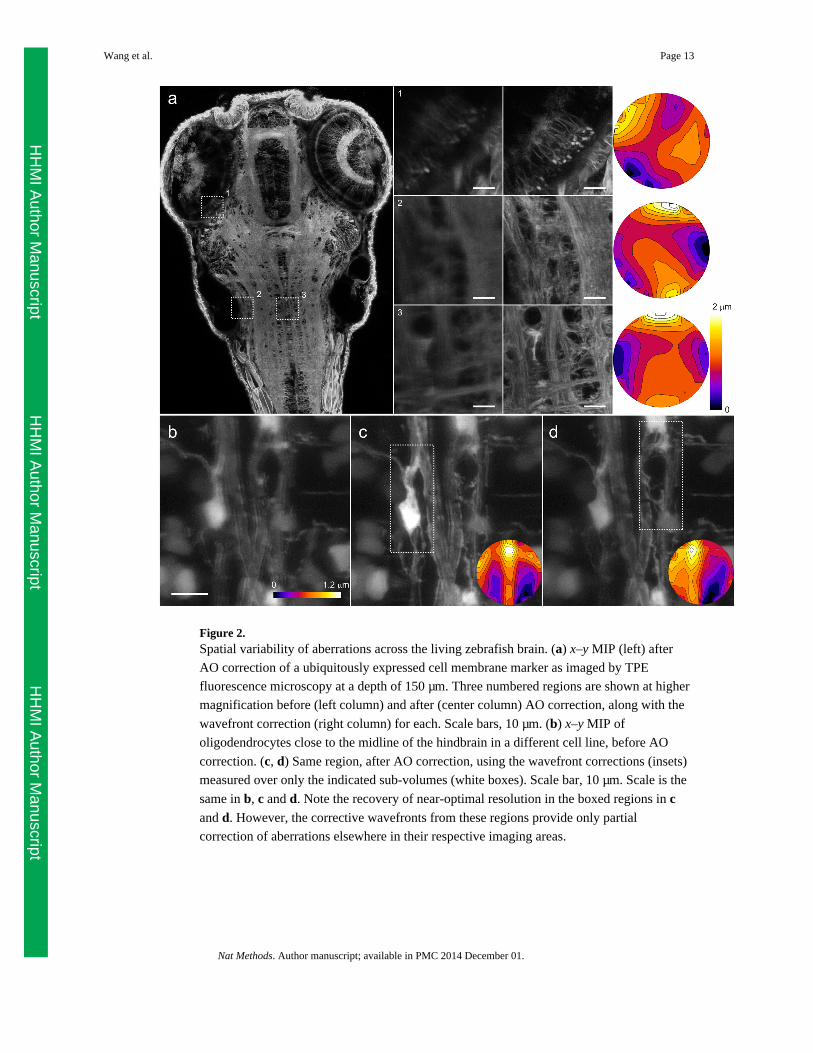
Figure 2.Spatial variability of aberrations across the living zebrafish brain. (a) x–y MIP (left) after

AO correction of a ubiquitously expressed cell membrane marker as imaged by TPE

fluorescence microscopy at a depth of 150 μm. Three numbered regions are shown at higher

magnification before (left column) and after (center column) AO correction, along with the

wavefront correction (right column) for each. Scale bars, 10 μm. (b) x–y MIP of

oligodendrocytes close to the midline of the hindbrain in a different cell line, before AO

correction. (c, d) Same region, after AO correction, using the wavefront corrections (insets)

measured over only the indicated sub-volumes (white boxes). Scale bar, 10 μm. Scale is the

same in b, c and d. Note the recovery of near-optimal resolution in the boxed regions in cand d. However, the corrective wavefronts from these regions provide only partial

correction of aberrations elsewhere in their respective imaging areas.

Wang et al.


HH

MI A

uthor Manuscript

HH

MI A

uthor Manuscript

HH

MI A

uthor Manuscript

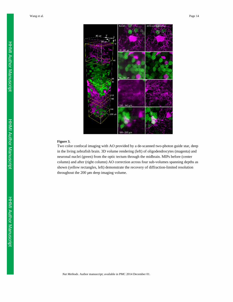
Figure 3.Two color confocal imaging with AO provided by a de-scanned two-photon guide star, deep

in the living zebrafish brain. 3D volume rendering (left) of oligodendrocytes (magenta) and

neuronal nuclei (green) from the optic tectum through the midbrain. MIPs before (center

column) and after (right column) AO correction across four sub-volumes spanning depths as

shown (yellow rectangles, left) demonstrate the recovery of diffraction-limited resolution

throughout the 200 μm deep imaging volume.

Wang et al.


HH

MI A

uthor Manuscript

HH

MI A

uthor Manuscript

HH

MI A

uthor Manuscript

Kai Wang Dan Milkie Ankur Saxena Peter Engerer Thomas...

Documents

Transcript of Kai Wang Dan Milkie Ankur Saxena Peter Engerer Thomas...