Journal of Differential Equations formulation for the ...lipeijun/paper/2013/Li_Zheng_2013.pdf ·...

Author's personal copy

J. Differential Equations 254 (2013) 3476–3500

Contents lists available at SciVerse ScienceDirect

Journal of Differential Equations

www.elsevier.com/locate/jde

An H-ψ formulation for the three-dimensional eddy currentproblem in laminated structures

Peijun Li a,1, Weiying Zheng b,∗,2

a Department of Mathematics, Purdue University, West Lafayette, IN, 47907, United Statesb NCMIS, LSEC, Academy of Mathematics and System Sciences, Chinese Academy of Sciences, Beijing, 100190, China

a r t i c l e i n f o a b s t r a c t

Article history:Received 11 January 2012Revised 9 October 2012Available online 5 February 2013

MSC:35K5535Q6078A25

Keywords:Eddy current problemH-ψ formulationNonlinear Maxwell’s equationsSilicon steel laminations

It is a very challenging problem for the direct simulation ofthe three-dimensional eddy currents in grain-oriented (GO) siliconsteel laminations since the coating film is only several micronsthick over each lamination and the magnetic permeability isnonlinear and anisotropic. In addition, the system of GO siliconsteel laminations has multiple scales and the ratio of the largestscale to the smallest scale can be up to 106. In this paper,we study an H-ψ formulation for the nonlinear eddy currentproblem in laminated conductors. By omitting the insulating filmsbetween neighboring laminations, we propose an approximatebut effective H-ψ formulation for the nonlinear eddy currentproblem, which reduces the scale ratio by 2–3 orders of magnitude.The well-posedness of the original problem and the approximateproblem are established by examining their weak formulations.The convergence is proved for the solution of the approximateproblem to the solution of the original problem as the thicknessof coating films approaches zero.

© 2013 Elsevier Inc. All rights reserved.

* Corresponding author.E-mail addresses: [email protected] (P. Li), [email protected] (W. Zheng).

1 The research was supported in part by the NSF grants DMS-0914595, DMS-1042958, and DMS-1151308.2 The research was supported in part by China NSF grants 11031006 and 11171334, by the Funds for Creative Research Groups

of China (Grant No. 11021101), by the National Magnetic Confinement Fusion Science Program (Grant No. 2011GB105003), andby National High Technology Research and Development Program of China (Grant No. 2012AA01A309).

0022-0396/$ – see front matter © 2013 Elsevier Inc. All rights reserved.http://dx.doi.org/10.1016/j.jde.2013.01.028


P. Li, W. Zheng / J. Differential Equations 254 (2013) 3476–3500 3477

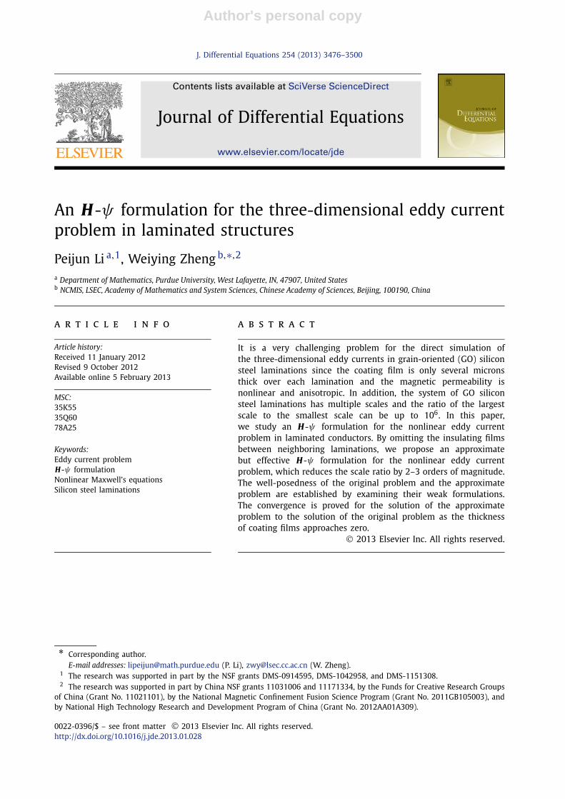
Fig. 1. A typical model of the eddy current problem.

1. Introduction

Consider the following eddy current problem for magnetic and anisotropic materials in terms ofFarady’s law and Ampere’s law:

∂ B

∂t+ curl E = 0 in R3, (1a)

curl H = J in R3, (1b)

where E is the electric field, B is the magnetic flux, H is the magnetic field, and J is the currentdensity defined by

J ={

σ E in Ωc,

J s in R3\Ωc.(2)

Eq. (1) is the eddy current model which approximates Maxwell’s equations at very low frequency byneglecting the displacement currents in Ampere’s law [1]. For magnetic materials, B = (B1, B2, B3)

is a nonlinear vector function of H = (H1, H2, H3) in the form of Bi = Bi(Hi), 1 � i � I , so that (1)is the nonlinear eddy current problem. And for nonmagnetic materials, B = μ0 H where μ0 is thepermeability in the empty space, and (1) stands for the linear eddy current problem. In (2), σ � 0 isthe electric conductivity, J s is the source current density carried by some coils and satisfies div J s = 0,Ωc denotes the conducting region, and the complement R3\Ωc denotes the nonconducting region(see Fig. 1). There are many works studying linear eddy current problems, e.g., on numerical methods[7,8,16,22,24,29], or on the regularity of the solution [17]. However, little has been done for themathematical and numerical analysis for nonlinear eddy current problems. We refer to Bachingeret al. [6] for the numerical analysis of nonlinear multi-harmonic eddy current problems in isotropicmaterials.

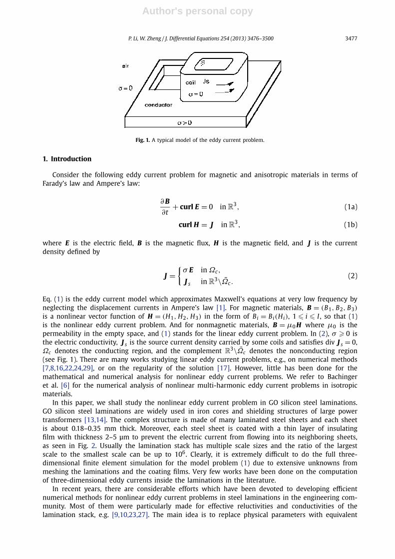
In this paper, we shall study the nonlinear eddy current problem in GO silicon steel laminations.GO silicon steel laminations are widely used in iron cores and shielding structures of large powertransformers [13,14]. The complex structure is made of many laminated steel sheets and each sheetis about 0.18–0.35 mm thick. Moreover, each steel sheet is coated with a thin layer of insulatingfilm with thickness 2–5 μm to prevent the electric current from flowing into its neighboring sheets,as seen in Fig. 2. Usually the lamination stack has multiple scale sizes and the ratio of the largestscale to the smallest scale can be up to 106. Clearly, it is extremely difficult to do the full three-dimensional finite element simulation for the model problem (1) due to extensive unknowns frommeshing the laminations and the coating films. Very few works have been done on the computationof three-dimensional eddy currents inside the laminations in the literature.

In recent years, there are considerable efforts which have been devoted to developing efficientnumerical methods for nonlinear eddy current problems in steel laminations in the engineering com-munity. Most of them were particularly made for effective reluctivities and conductivities of thelamination stack, e.g. [9,10,23,27]. The main idea is to replace physical parameters with equivalent


3478 P. Li, W. Zheng / J. Differential Equations 254 (2013) 3476–3500

Fig. 2. GO silicon steel laminations. (Left) the magnetic shield for protecting the magnetic plate; (Right) the magnetic shieldmade of laminated steel sheets.

(or homogenized) parameters for Maxwell’s equations. In [11,12], Bottauscio et al. proposed a mathe-matical homogenization technique based on the multi-scale expansion theory to derive the equivalentelectric parameters and effective magnetization properties. In [19,20], Gyselinck et al. deduced theeffective material parameters by an orthogonal decomposition of the flux in the perpendicular andparallel directions to the lamination plane. In [21], Napieralska-Juszczak et al. established equivalentcharacteristics of magnetic joints of transformer cores by minimizing the magnetic energy of the sys-tem. In [25], Nédélec and Wolf studied the homogenization method for eddy currents in a transformercore and proved the convergence of the exact solution to the solution of the homogenized problemas the thickness of the steel sheet approaches zero. Numerical methods based on the homogenizationof material parameters provide an efficient way to simulate electromagnetic field in steel laminations.In [2], Ammari and Nédélec studied the electromagnetic scattering problem by a perfectly conductingobject coated with a thin chiral curved layer. They proposed the approximate impedance conditionwithout modeling the exact fields inside the thin layer and proved optimal error estimates. In [3],Ammari et al. studied the electromagnetic scattering by a thin dielectric planar structure. The approx-imate solution of Maxwell’s equations comprises both the leading term and a first-order correction.We also refer to [4] for the asymptotic analysis of nonlinear Maxwell’s equations with thin ferromag-netic films.

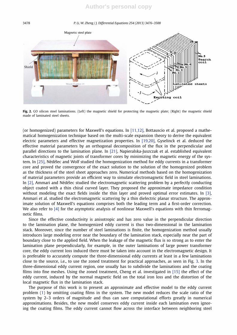
Since the effective conductivity is anisotropic and has zero value in the perpendicular directionto the lamination plane, the homogenized eddy current is thus two-dimensional in the laminationstack. Moreover, since the number of steel laminations is finite, the homogenization method usuallyintroduces large modeling error near the boundary of the lamination stack, especially near the part ofboundary close to the applied field. When the leakage of the magnetic flux is so strong as to enter thelamination plane perpendicularly, for example, in the outer laminations of large power transformercore, the eddy current loss induced there must be taken into account in the electromagnetic design. Itis preferable to accurately compute the three-dimensional eddy currents at least in a few laminationsclose to the source, i.e., to use the zoned treatment for practical approaches, as seen in Fig. 3. In thethree-dimensional eddy current region, one usually has to subdivide the laminations and the coatingfilms into fine meshes. Using the zoned treatment, Cheng et al. investigated in [15] the effect of theeddy current, induced by the normal magnetic field on the total iron loss and the distortion of thelocal magnetic flux in the lamination stack.

The purpose of this work is to present an approximate and effective model to the eddy currentproblem (1) by omitting coating films in the system. The new model reduces the scale ratio of thesystem by 2–3 orders of magnitude and thus can save computational efforts greatly in numericalapproximations. Besides, the new model conserves eddy current inside each lamination even ignor-ing the coating films. The eddy current cannot flow across the interface between neighboring steel



Fig. 3. Zoned treatment of the lamination stack. The six laminations close to the source are treated with three-dimensionalsimulations while the other laminations are treated with homogenization methods.

laminations. Specifically, we obtained the following results for Maxwell’s equations of the nonlineareddy current problem:

1. We proved the existence and uniqueness of both the exact solution and the approximate solutionfor the original and the approximate problems. We developed some new techniques to handle thenonlinearity in the mathematical analysis of Maxwell’s equations. To the best of our knowledge,this is the first work studying the well-posedness of the H -ψ formulation for nonlinear andtime-dependent eddy current problems.

2. We proved the stability of the exact and the approximate solutions to the original and the ap-proximate problems with respect to the source current.

3. We proved that the approximate solution converges strongly to the exact solution in the L2-normas the thickness of the coating film approaches zero.

4. For the linear eddy current problem, we deduced an explicit error estimate between the approx-imate solution and the exact solution with respect to the thickness of the coating film.

The layout of the paper is as follows. In Section 2, we present some notation and Sobolev spacesand study the H -ψ formulation for the model problem (1). The well-posedness of the nonlinear eddycurrent problem is established in Section 3. Section 4 is devoted to the well-posedness of the solutionfor an approximate H -ψ formulation of the nonlinear eddy current problem by omitting coating films.The convergence is examined in Section 5 for the approximate solution to the exact solution as thethickness of the coating film tends to zero.

2. The H -ψ formulation of eddy current problem

Let Ω ⊂ R3 be a sufficiently large, bounded, and convex polyhedral domain containing all conduc-tors and coils. Denote the conducting domain by Ωc which consists of all conductors. Let Ωnc = Ω\Ωc

be the nonconducting domain such that σ ≡ 0 in Ωnc . Throughout the paper, we make the followingassumptions on the electric conductivity and the nonlinear relationship between H = (H1, H2, H3)

and B = (B1, B2, B3) which are usually satisfied in electrical engineering:

(H1) The conductivity σ is a piecewise constant in Ω . There exist two constants σmin and σmax suchthat

0 < σmin � σ � σmax in Ωc.

(H2) Bi is a Lipschitz continuous function of Hi satisfying Bi(Hi) = μ0 Hi in Ωnc and Bi(0) = 0. Thereexist two constants μmin and μmax such that

0 < μmin � B ′i(Hi) � μmax a.e. in Ω, i = 1,2,3.



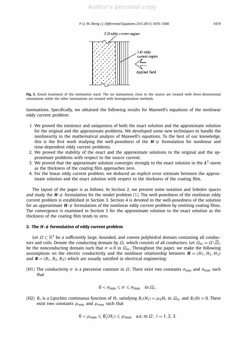
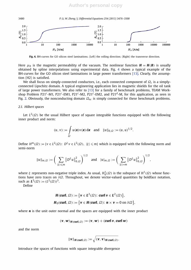
Fig. 4. BH-curves for GO silicon steel laminations. (Left) the rolling direction; (Right) the transverse direction.

Here μ0 is the magnetic permeability of the vacuum. The nonlinear function H = H(B) is usuallyobtained by spline interpolations using experimental data. Fig. 4 shows a typical example of theBH-curves for the GO silicon steel laminations in large power transformers [13]. Clearly, the assump-tion (H2) is satisfied.

We shall focus on simply-connected conductors, i.e., each connected component of Ωc is a simply-connected Lipschitz domain. A typical engineering application lies in magnetic shields for the oil tankof large power transformers. We also refer to [13] for a family of benchmark problems, TEAM Work-shop Problem P21c-M1, P21c-EM1, P21c-M2, P21c-EM2, and P21d-M, for this application, as seen inFig. 2. Obviously, the nonconducting domain Ωnc is simply connected for these benchmark problems.

2.1. Hilbert spaces

Let L2(Ω) be the usual Hilbert space of square integrable functions equipped with the followinginner product and norm:

(u, v) :=∫Ω

u(x)v(x)dx and ‖u‖0,Ω := (u, u)1/2.

Define Hm(Ω) := {v ∈ L2(Ω): Dξ v ∈ L2(Ω), |ξ | � m} which is equipped with the following norm andsemi-norm

‖u‖m,Ω :=( ∑

|ξ |�m

∥∥Dξ u∥∥2

0,Ω

)1/2

and |u|m,Ω :=( ∑

|ξ |=m

∥∥Dξ u∥∥2

0,Ω

)1/2

,

where ξ represents non-negative triple index. As usual, H10(Ω) is the subspace of H1(Ω) whose func-

tions have zero traces on ∂Ω . Throughout, we denote vector-valued quantities by boldface notation,such as L2(Ω) := (L2(Ω))3.

Define

H(curl,Ω) := {v ∈ L2(Ω): curl v ∈ L2(Ω)

},

H 0(curl,Ω) := {v ∈ H(curl,Ω): n × v = 0 on ∂Ω

},

where n is the unit outer normal and the spaces are equipped with the inner product

(v, w)H(curl,Ω) := (v, w) + (curl v, curl w)

and the norm

‖v‖H(curl,Ω) :=√

(v, v)H(curl,Ω).

Introduce the spaces of functions with square integrable divergence



H(div,Ω) := {v ∈ L2(Ω): div v ∈ L2(Ω)

},

H 0(div,Ω) := {v ∈ H(div,Ω): n · v = 0 on ∂Ω

},

which are equipped with the inner product

(v, w)H(div,Ω) := (v, w) + (div v,div w)

and the norm

‖v‖H(div,Ω) :=√

(v, v)H(div,Ω).

To study the weak solution of (1), we shall use the subspaces of H(curl,Ω):

X := ∇H1(Ω) + H 0(curl,Ωc), (3)

Xc := {v ∈ H 0(curl,Ωc): div v = 0 in Ωc

}. (4)

It is easy to see that

‖v‖2H(curl,Ω) = ‖v‖2

L2(Ω)+ ‖curl v‖2

L2(Ωc)for all v ∈ X .

We shall use the convention that all functions in H 0(curl, D) and H10(D) are extended by zero to the

exterior of D for any D ⊂ Ω .

Lemma 2.1. Let the nonconducting region Ωnc be simply connected. Then

X = {v ∈ H(curl,Ω): curl v = 0 in Ωnc

}.

Furthermore, for any v ∈ X , there exist a unique vc ∈ Xc and a unique φ ∈ H1(Ω)/R such that

v = vc + ∇φ, ‖vc‖H(curl,Ω) + ‖φ‖H1(Ω) � C‖v‖H(curl,Ω),

where C > 0 is a constant only depending on Ωnc .

Proof. It is clear that X ⊂ {v ∈ H(curl,Ω): curl v = 0 in Ωnc}.Suppose that v ∈ H(curl,Ω) and satisfies curl v = 0 in Ωnc . Since Ωnc is simply connected, the

potential theorem [5] shows that v = ∇φnc in Ωnc for some φnc ∈ H1(Ωnc). By Stein’s extensiontheorem [28], there exist a φ1 ∈ H1(Ω) and a constant C only depending on Ωnc such that

φ1 = φnc in Ωnc and ‖φ1‖H1(Ω) � C‖φnc‖H1(Ωnc)� C‖v‖L2(Ω). (5)

Clearly v1 := v − ∇φ1 ∈ H 0(curl,Ωc) and satisfies

‖v1‖H(curl,Ω) � C(‖φ1‖H1(Ω) + ‖v‖H(curl,Ω)

)� C‖v‖H(curl,Ω). (6)

Thus v = v1 + ∇φ1 ∈ X and {v ∈ H(curl,Ω): curl v = 0 in Ωnc} ⊂ X .



Now suppose that v = v1 + ∇φ1 with v1 ∈ H 0(curl,Ωc) and φ1 ∈ H1(Ω)/R. Let φ2 ∈ H10(Ωc) be

the unique solution of the following elliptic problem:

∫Ωc

∇φ2 · ∇ϕ =∫Ωc

v1 · ∇ϕ for all ϕ ∈ H10(Ωc).

Then v = vc + ∇φ with vc := v1 − ∇φ2 ∈ Xc and φ := φ1 + φ2 ∈ H1(Ω)/R. Combining (5) and (6)yields that

‖vc‖H(curl,Ω) � 2‖v1‖H(curl,Ω) � C‖v‖H(curl,Ω)

and

‖φ‖H1(Ω) � C‖∇φ‖L2(Ω) � C‖v − vc‖L2(Ω) � C‖v‖H(curl,Ω).

To prove the uniqueness, we let v = vc + ∇φ be another decomposition with vc ∈ Xc and φ ∈H1(Ω)/R. Then vc − vc ∈ H 0(curl,Ωc) and satisfies

div(vc − vc) = 0, curl(vc − vc) = 0 in Ωc.

It follows from [5] that vc = vc and thus φ = φ. �2.2. The weak formulation

Since div J s ≡ 0, there exists a source magnetic field H s such that

J s = curl H s in R3. (7)

The field H s can be written explicitly by the Biot–Savart law for general coils

H s := curl As,

where

As(x) := 1

4π

∫R3

J s(y)

|x − y| d y.

Denote the residual H r := H − H s , which is also called the reaction field in [18]. Using (1) and (7),we have curl H r = 0 in Ωnc . A direct application of Lemma 2.1 yields the following result.

Lemma 2.2. The reaction field H r ∈ H(curl,Ω) admits a unique decomposition

H r = u + ∇ψ, u ∈ Xc, ψ ∈ H1(Ω)/R. (8)



Next we deduce a weak formulation of (1). For any v ∈ X , (1a) implies that∫Ωc

∂ B

∂t· v = −

∫Ωc

curl E · v = −∫Ωc

E · curl v +∫

∂Ωc

(E × nc) · v

=∫Ωc

σ−1( J s − curl H) · curl v +∫

∂Ωc

(E × nc) · v, (9)

∫Ωnc

∂ B

∂t· v = −

∫Ωnc

curl E · v =∫

∂Ωnc

(E × nnc) · v, (10)

where nc , nnc are the unit outer normals to ∂Ωc and ∂Ωnc respectively. Noting the tangential conti-nuity of E and v across ∂Ωc and the fact that

σ−1( J s − curl H) = −σ−1 curl H r in Ωc,

we add (9) and (10) and obtain∫Ω

∂ B

∂t· v +

∫Ωc

σ−1 curl H r · curl v = 0 for all v ∈ X . (11)

For convenience, we shall drop the subscript of H r and let H denote the reaction field in the rest ofthe paper, and define

σ1 ={

σ−1 in Ωc,

0 in Ωnc.

Using (11) and viewing B as a nonlinear vector function of the total magnetic field, we obtain aweak formulation of (1): Find H ∈ X such that H(·,0) = 0 and∫

Ω

∂

∂tB(H + H s) · v +

∫Ω

σ1 curl H · curl v = 0 for all v ∈ X . (12)

3. Well-posedness of the weak formulation

We shall use Rothe’s method (cf. [26]) to study the weak solution. Let N be a positive integerand {tn = nτ : n = 0, . . . , N} be an equidistant partition of [0, T ] with τ = T /N . The semi-discreteapproximation to (12) reads: Given H 0 = 0, find Hn ∈ X , 1 � n � N , such that∫

Ω

Bn − Bn−1

τ· v +

∫Ω

σ1 curl Hn · curl v = 0 for all v ∈ X, (13)

where Bn := B(Hn + H s(tn)).We define the piecewise constant and piecewise linear interpolations in time by

Hτ (·, t) = Hn, Hτ (·, t) = ln(t)Hn + (1 − ln(t)

)Hn−1,

Bτ (·, t) = Bn, Bτ (·, t) = ln(t)Bn + (1 − ln(t)

)Bn−1, (14)



for any t ∈ (tn−1, tn] and 1 � n � N , where

ln(t) := τ−1(t − tn−1).

Clearly we have

Hτ ∈ L2(0, T ; X), Hτ ∈ C(0, T ; X),

Bτ ∈ L2(0, T ; L2(Ω)), Bτ ∈ C

(0, T ; L2(Ω)

).

The following lemma is concerned with the well-posedness of the weak formulation (13).The proof is given in Appendix A.

Lemma 3.1. For any 1 � n � N, the weak formulation (13) has a unique solution Hn ∈ X . Suppose thatH s ∈ H 1(0, T ; L2(Ω)). Then there exists a constant C only depending on Ωc , T , μmax , μmin , σmax , σmin suchthat

‖Hτ ‖H 1(0,T ;L2(Ω)) + ‖curl Hτ ‖L∞(0,T ;L2(Ω)) � C‖H s‖H 1(0,T ;L2(Ω)), (15)

‖Hτ ‖L2(0,T ;L2(Ω)) + ‖curl Hτ ‖L∞(0,T ;L2(Ω)) � C‖H s‖H 1(0,T ;L2(Ω)), (16)

‖Bτ ‖L2(0,T ;L2(Ω)) + ‖Bτ ‖H 1(0,T ;L2(Ω)) � C‖H s‖H 1(0,T ;L2(Ω)). (17)

It follows from Lemma 2.1 that each Hn admits the decomposition in a direct sum

Hn = un + ∇ψn, un ∈ Xc, ψn ∈ H1(Ω)/R.

For any t ∈ (tn−1, tn] and 1 � n � N , we may define uτ ∈ L2(0, T ; X c) and uτ ∈ C(0, T ; Xc) by us-ing {un}:

uτ (·, t) = un, uτ (·, t) = ln(t)un + (1 − ln(t)

)un−1, (18)

which gives the decompositions

Hτ = uτ + ∇ψτ , Hτ = uτ + ∇ψτ .

Here ψτ and ψτ are defined as

ψτ (·, t) := ψn, ψτ (·, t) := ln(t)ψn + (1 − ln(t)

)ψn−1,

for all t ∈ (tn−1, tn] and 1 � n � N .Introduce the Sobolev–Bochner space (cf. [26, Section 7.1])

W 1,2,2(0, T ; H 1(Ω), L2(Ω)) :=

{v ∈ L2(0, T ; H 1(Ω)

):

∂ v

∂t∈ L2(0, T ; L2(Ω)

)},

which is equipped with the following norm

‖v‖W 1,2,2(0,T ;H 1(Ω),L2(Ω)) =(

‖v‖2L2(0,T ;H 1(Ω))

+∥∥∥∥∂ v

∂t

∥∥∥∥2

L2(0,T ;L2(Ω))

)1/2

.



Next we examine the convergence of the temporally discrete functions. For convenience, we shall usethe same notation to denote their subsequences without causing confusion.

Lemma 3.2. Assume that each connected component of Ωc is a convex polyhedron. Then uτ ∈ W 1,2,2(0, T ;H 1(Ωc), L2(Ωc)) and satisfies

‖uτ ‖L2(0,T ;H 1(Ωc))+ ‖uτ ‖W 1,2,2(0,T ;H 1(Ωc),L2(Ωc))

� C‖H s‖H 1(0,T ;L2(Ω)). (19)

Furthermore, there exist a subsequence of {uτ }τ�0 , a subsequence of {uτ }τ�0 , and a u ∈ L2(0, T ; Xc) suchthat

limτ→0

‖uτ − u‖L2(0,T ;L2(Ωc))= lim

τ→0‖uτ − u‖L2(0,T ;L2(Ωc))

= 0. (20)

Proof. Since each connected component of Ωc is a convex polyhedron, we know that H 0(curl,Ωc) ∩H(div,Ωc) ⊂ H 1(Ωc) (cf. e.g., [5]). This implies un ∈ H 1(Ωc) and

‖un‖H 1(Ωc)� C

{‖un‖H(curl,Ωc) + ‖div un‖L2(Ωc)

}� C‖Hn‖H(curl,Ω), (21)

where we have used Lemma 2.1 and the fact that div un = 0 in Ωc in the last inequality. Then (19)follows from (15).

By the compact embedding (cf. [26, Lemma 7.7])

W 1,2,2(0, T ; H 1(Ωc), L2(Ωc))� L2(0, T ; L2(Ωc)

),

there exist a subsequence of {uτ }τ�0 and a u ∈ W 1,2,2(0, T ; H 1(Ωc), L2(Ωc)) such that

limτ→0

uτ = ustrongly in L2

(0, T ; L2(Ωc)

),

weakly in W 1,2,2(0, T ; H 1(Ωc), L2(Ωc)

).

The weak convergence of {uτ }τ�0 indicates that, for any v ∈ L2(0, T ; H 1(Ωc)),

T∫0

∫∂Ωc

(u × n) · v =T∫

0

∫Ωc

(u · curl v − curl u · v) = limτ→0

T∫0

∫Ωc

(uτ · curl v − curl uτ · v)

= limτ→0

T∫0

∫∂Ωc

(uτ × n) · v = 0.

We conclude that u ∈ L2(0, T ; H 0(curl,Ωc)). Since div uτ = 0, it is clear that

T∫0

∫Ωc

u · ∇ϕ = limτ→0

T∫0

∫Ωc

uτ · ∇ϕ = 0 for all ϕ ∈ L2(0, T ; H10(Ωc)

),

which shows div u = 0 and thus u ∈ L2(0, T ; Xc).



Finally we deduce from (19) and the strong convergence of uτ that

limτ→0

‖uτ − u‖2L2(0,T ;L2(Ωc))

� limτ→0

‖uτ − uτ ‖2L2(0,T ;L2(Ωc))

= limτ→0

N∑n=1

τ

3‖un − un−1‖2

L2(Ωc)

= limτ→0

τ 2

3

∥∥∥∥∂uτ

∂t

∥∥∥∥2

L2(0,T ;L2(Ωc))

= 0,

which completes the proof. �Lemma 3.3. Let (H1)–(H2) be satisfied. Assume that each connected component of Ωc is a convex polyhedronand

limτ→0

‖H s,τ − H s‖L2(0,T ;L2(Ω)) = 0, (22)

where H s,τ is the piecewise constant interpolation of H s in time

H s,τ (·, t) = H s(·, tn) for all t ∈ (tn−1, tn], 1 � n � N.

Then there exists an H ∈ L2(0, T ; X) such that

limτ→0

Hτ = limτ→0

Hτ = Hstrongly in L2

(0, T ; L2(Ω)

),

weakly in L2(0, T ; X).

Proof. Since L2(0, T ; X) is self-reflective, by (16), there exist a subsequence of {Hτ }τ�0 and a subse-quence of {Hτ }τ�0 such that

limτ→0

Hτ = limτ→0

Hτ = H weakly in L2(0, T ; X).

By Lemma 2.1, H can be decomposed into H = u + ∇ψ where ψ ∈ H1(Ω)/R and u is the limitof uτ .

Next we prove the strong convergence of Hτ . The strong convergence of Hτ comes directly fromthat of Hτ . For convenience we denote the discrete and continuous total magnetic fields by Hτ =Hτ + H s,τ and H = H + H s respectively. It follows from (22) and the weak convergence of Hτ that

limτ→0

Hτ = H weakly in L2(0, T , L2(Ω)). (23)

From (13) and (14) we deduce that

(Bτ ,∇ϕ) = 0 for all ϕ ∈ H1(Ω).

Then using Lemmas 3.1–3.2 and (22), we obtain

limτ→0

T∫0

(Bτ , Hτ − H) = limτ→0

T∫0

(Bτ , uτ − u + H s,τ − H s) = 0. (24)

Noting the monotonicity of B(·) and using (23)–(24), we have



μmin limτ→0

‖Hτ − H‖2L2(0,T ;L2(Ω))

� limτ→0

T∫0

(B(Hτ ) − B(H), Hτ − H

)

= limτ→0

T∫0

(Bτ , Hτ − H) − limτ→0

T∫0

(B(H), Hτ − H

) = 0,

which shows together with (22) that limτ→0 ‖Hτ − H‖2L2(0,T ;L2(Ω))

= 0. �Theorem 3.1. Let (H1)–(H2) be satisfied. Furthermore, assume that each connected component of Ωc is aconvex polyhedron, and H s ∈ H 1(0, T ; L2(Ω)) satisfies (22) and H s|t=0 = 0. Then (12) has a unique solutionH ∈ H 1(0, T ; X), and there exists a constant C only depending on Ωc , T , μmax , μmin , σmax , σmin such that

‖H‖H 1(0,T ;L2(Ω)) + ‖H‖L2(0,T ;H(curl,Ω)) � C‖H s‖H 1(0,T ;L2(Ω)).

Proof. Using (14), we first write (13) into the following equation

T∫0

(∂ Bτ

∂t, v

)+

T∫0

(σ1 curl Hτ , curl v) = 0 for all v ∈ L2(0, T ; X). (25)

Since H 1(0, T ; L2(Ω)) is self-reflective, by (17), {Bτ }τ�0 has a subsequence satisfying

limτ→0

Bτ = B0 weakly in H 1(0, T ; L2(Ω)), (26)

which implies that

limτ→0

Bτ = B0 weakly in L2(0, T ; L2(Ω)).

Write Hτ := Hτ + H s,τ and H := H + H s , where H is the limit of Hτ in Lemma 3.3. Due to thestrong convergence of Hτ and H s,τ , it is easy to show that

limτ→0

‖Hτ − H‖L2(0,T ;L2(Ω)) = 0.

Using (H2), we deduce that

limτ→0

∥∥Bτ − B(H + H s)∥∥

L2(0,T ;L2(Ω))= lim

τ→0

∥∥B(Hτ ) − B(H)∥∥

L2(0,T ;L2(Ω))

� μmax limτ→0

‖Hτ − H‖L2(0,T ;L2(Ω)) = 0.

Thus we have B0 = B(H + H s).Since σ1 is bounded and positive in Ωc , the weak convergence of Hτ in L2(0, T ; X) shows that

limτ→0

T∫0

(σ1 curl Hτ , curl v) =T∫

0

(σ1 curl H , curl v) for all v ∈ L2(0, T ; X). (27)



Plugging (26) and (27) into (25) lead to

T∫0

(∂

∂tB(H + H s), v

)+

T∫0

(σ1 curl H , curl v) = 0 for all v ∈ L2(0, T ; X). (28)

Therefore (12) holds in the sense of distribution.Next we prove the initial condition. We write B = B(H + H s) for convenience and take any ϕ ∈

C1([0, T ]) satisfying ϕ(0) = 1 and ϕ(T ) = 0. By (26) and integration by parts, we deduce that

(B|t=0, v) =T∫

0

{ϕ(t) · ∂

∂t(B, v) + ϕ′(t) · (B, v)

}dt

= limτ→0

T∫0

{ϕ(t) · ∂

∂t(Bτ , v) + ϕ′(t) · (Bτ , v)

}dt

= limτ→0

(Bτ |t=0, v) = (B(H 0 + H s|t=0), v

) = 0 for all v ∈ L2(Ω).

Thus B|t=0 = 0. Since H s|t=0 = 0, by (H2) we have H |t=0 = 0.The stability estimates for H are easy. In fact, from Lemma 3.1, there exists a subsequence of

{Hτ }τ�0 which converges to H weakly in both H 1(0, T ; L2(Ω)) and L2(0, T ; X). Then (15) showsthat ∥∥∥∥∂ H

∂t

∥∥∥∥L2(0,T ;L2(Ω))

+ ‖H‖L2(0,T ;H(curl,Ω))

� limτ→0

{∥∥∥∥∂ Hτ

∂t

∥∥∥∥L2(0,T ;L2(Ω))

+ ‖Hτ ‖L2(0,T ;H(curl,Ω))

}� C‖H s‖H 1(0,T ;L2(Ω)),

which completes the proof. �4. The approximate formulation without coating films

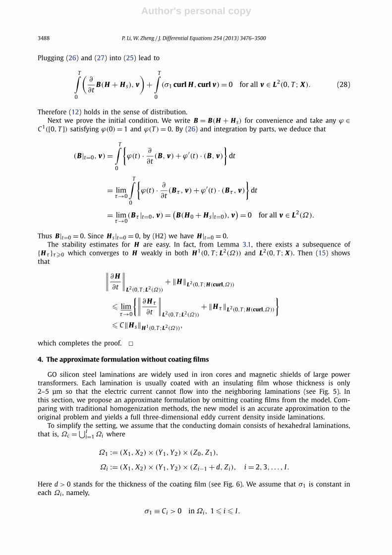
GO silicon steel laminations are widely used in iron cores and magnetic shields of large powertransformers. Each lamination is usually coated with an insulating film whose thickness is only2–5 μm so that the electric current cannot flow into the neighboring laminations (see Fig. 5). Inthis section, we propose an approximate formulation by omitting coating films from the model. Com-paring with traditional homogenization methods, the new model is an accurate approximation to theoriginal problem and yields a full three-dimensional eddy current density inside laminations.

To simplify the setting, we assume that the conducting domain consists of hexahedral laminations,that is, Ωc = ⋃I

i=1 Ωi where

Ω1 := (X1, X2) × (Y1, Y2) × (Z0, Z1),

Ωi := (X1, X2) × (Y1, Y2) × (Zi−1 + d, Zi), i = 2,3, . . . , I.

Here d > 0 stands for the thickness of the coating film (see Fig. 6). We assume that σ1 is constant ineach Ωi , namely,

σ1 ≡ Ci > 0 in Ωi, 1 � i � I.



Fig. 5. Geometric size of silicon steel laminations in Team Workshop Problem 21c -M1 [13].

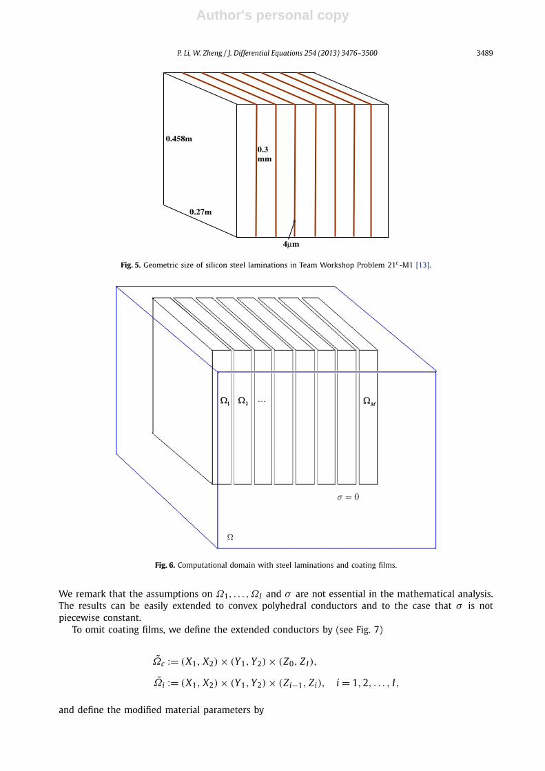
Fig. 6. Computational domain with steel laminations and coating films.

We remark that the assumptions on Ω1, . . . ,ΩI and σ are not essential in the mathematical analysis.The results can be easily extended to convex polyhedral conductors and to the case that σ is notpiecewise constant.

To omit coating films, we define the extended conductors by (see Fig. 7)

Ωc := (X1, X2) × (Y1, Y2) × (Z0, Z I ),

Ωi := (X1, X2) × (Y1, Y2) × (Zi−1, Zi), i = 1,2, . . . , I,

and define the modified material parameters by



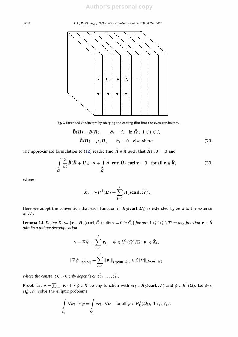
Fig. 7. Extended conductors by merging the coating film into the even conductors.

B(H) = B(H), σ1 = Ci in Ωi, 1 � i � I,

B(H) = μ0 H , σ1 = 0 elsewhere. (29)

The approximate formulation to (12) reads: Find H ∈ X such that H(·,0) = 0 and∫Ω

∂

∂tB(H + H s) · v +

∫Ω

σ1 curl H · curl v = 0 for all v ∈ X, (30)

where

X := ∇H1(Ω) +I∑

i=1

H 0(curl, Ωi).

Here we adopt the convention that each function in H 0(curl, Ωi) is extended by zero to the exteriorof Ωi .

Lemma 4.1. Define X i := {v ∈ H 0(curl, Ωi): div v = 0 in Ωi} for any 1 � i � I . Then any function v ∈ Xadmits a unique decomposition

v = ∇ψ +I∑

i=1

v i, ψ ∈ H1(Ω)/R, v i ∈ X i,

‖∇ψ‖L2(Ω) +I∑

i=1

‖v i‖H(curl,Ωi)� C‖v‖H(curl,Ω),

where the constant C > 0 only depends on Ω1, . . . , ΩI .

Proof. Let v = ∑Ii=1 w i + ∇φ ∈ X be any function with w i ∈ H 0(curl, Ωi) and φ ∈ H1(Ω). Let φi ∈

H10(Ωi) solve the elliptic problems∫

Ωi

∇φi · ∇ϕ =∫Ωi

w i · ∇ϕ for all ϕ ∈ H10(Ωi), 1 � i � I.



Then we have v = ∑Ii=1 v i + ∇ψ with v i := w i − ∇φi ∈ X i and ψ = φ + ∑I

i=1 φi ∈ H1(Ω). ThePoincaré-type inequality [5] shows that

‖v i‖H(curl,Ω) � C‖curl v i‖L2(Ωi)= C‖curl w i‖L2(Ωi)

= C‖curl v‖L2(Ωi),

‖∇ψ‖L2(Ω) � ‖v‖L2(Ω) +I∑

i=1

‖v i‖L2(Ω) � C‖v‖L2(Ω),

where the constant C only depends on Ωi . The uniqueness of the decomposition follows from thestability estimate. �Theorem 4.1. Let (H1)–(H2) be satisfied and let H s ∈ H 1(0, T ; L2(Ω)) satisfy (22) and H s(·,0) = 0. Then(30) has a unique solution H ∈ H 1(0, T ; X) and

‖H‖H 1(0,T ;L2(Ω)) + ‖H‖L2(0,T ;H(curl,Ω)) � C‖H s‖H 1(0,T ;L2(Ω)).

Proof. The proof is similar to that of Lemma 3.1. We omit the details here. �5. Convergence of the approximate solution

This section is to show that the solution of (12) converges to the solution of (30) as the thicknessof the coating film tends to zero. For simplicity, we assume that d = dist(Ωi;Ωi+1) is constant for all1 � i < I and denote the solution of (12) by H (d) . We first consider the convergence for the nonlineareddy current problem, and then deduce an explicit error estimate for the linear eddy current problem.

5.1. Convergence for the nonlinear eddy current problem

We begin with a useful lemma.

Lemma 5.1. There exists an H (0) ∈ L2(0, T ; X) such that

limd→0

H (d) = H (0) strongly in L2(0, T ; L2(Ω))

and weakly in L2(0, T ; X).

Proof. Since Ωi ⊂ Ωi , we have H 0(curl,Ωi) ⊂ H 0(curl, Ωi) for all 1 � i � I and thus X ⊂ X . Weinfer from (16) that {H (d)}d>0 constructs a bounded sequence in L2(0, T ; X). Then there exists asubsequence still denoted by {H (d)}d>0 such that

limd→0

H (d) = H (0) weakly in L2(0, T ; X).

It follows from Lemma 4.1 that H (d) and H (0) can be decomposed uniquely into

H (d) =I∑

i=1

u(d)i + ∇ψ(d), H (0) =

I∑i=1

u(0)i + ∇ψ(0),

where u(d)i , u(0)

i ∈ L2(0, T ; X i) and ψ(d),ψ(0) ∈ H1(Ω)/R. The uniqueness of the decompositions indi-cates that

limd→0

u(d)i = u(0)

i weakly in L2(0, T ; X i).



Using Theorem 3.1 and the stability of the decompositions, we have

I∑i=1

∥∥∥∥∂u(d)i

∂t

∥∥∥∥L2(0,T ;L2(Ω))

+I∑

i=1

∥∥u(d)i

∥∥L2(0,T ;H(curl,Ω))

� C‖H s‖H 1(0,T ;L2(Ω)).

The embedding of H 0(curl, Ωi) ∩ H(div, Ωi) ⊂ H 1(Ωi) [5] shows that

I∑i=1

∥∥u(d)i

∥∥W 1,2,2(0,T ;H 1(Ωi),L2(Ωi))

� C‖H s‖H 1(0,T ;L2(Ω)).

By the compact embedding W 1,2,2(0, T ; H 1(Ωi), L2(Ωi)) � L2(0, T ; L2(Ωi)), there exists a subse-quence still denoted by {u(d)

i }d>0 such that

limd→0

u(d)i = u(0)

i

strongly in L2(0, T ; L2(Ωi)

),

weakly in W 1,2,2(0, T ; H 1(Ωi), L2(Ωi)

).

Define B(d) := B(H (d) + H s). Taking test functions from ∇H1(Ω) in (12) shows that

(B(d),∇ϕ

) = 0 for all ϕ ∈ H1(Ω).

We have from assumption (H2) that

μmin limd→0

∥∥H (d) − H (0)∥∥2

L2(0,T ;L2(Ω))

� limd→0

T∫0

(B(d) − B(0), H (d) − H (0)

)

= limd→0

I∑i=1

T∫0

∫Ωi

B(d) · (u(d)i − u(0)

i

) − limd→0

T∫0

(B(0), H (d) − H (0)

) = 0,

where we have used the strong convergence of u(d)i and the weak convergence of H (d) in the last

equality. This completes the proof. �Theorem 5.1. Let (H1)–(H2) be satisfied and let H (d), H be the solutions of (12) and (30) respectively. Then

limd→0

∥∥H (d) − H∥∥

L2(0,T ;L2(Ω))= 0.

Proof. Denote B(d) := B(H (d) + H s) and B(d) := B(H (d) + H s) for any d � 0, where B is defined

in (29). Following from (H2) and Theorem 3.1, we have

∥∥B(d)∥∥

H 1(0,T ;L2(Ω))� C

∥∥H (d) + H s∥∥

H 1(0,T ;L2(Ω))� C‖H s‖H 1(0,T ;L2(Ω)). (31)



Since H 1(0, T ; L2(Ω)) is self-reflective, there exist a B0 ∈ H 1(0, T ; L2(Ω)) and a subsequence of

{B(d)}d>0 such that

limd→0

B(d) = B0 weakly in H 1(0, T ; L2(Ω)

). (32)

Using assumption (H2) and Lemma 5.1, we obtain that

limd→0

∥∥B(d) − B

(0)∥∥L2(0,T ;L2(Ω))

� μmax limd→0

∥∥H (d) − H (0)∥∥

L2(0,T ;L2(Ω))= 0,

where H (0) is the limit of H (d) in Lemma 5.1. Thus we conclude that

B0 = B(0) = B

(H (0) + H s

).

Noting the measure (Ωi\Ω i) → 0 as d → 0, we have from (31) that

limd→0

T∫0

∫Ωi\Ω i

∂

∂t

(B(d) − B

(d)) · v = 0 for all v ∈ L2(0, T ; L2(Ω)),

which implies that

limd→0

T∫0

(∂

∂tB(d), v

)= lim

d→0

T∫0

(∂

∂tB

(d), v

)for all v ∈ L2(0, T ; L2(Ω)

). (33)

From (12) and supp(curl H (d)) = supp(σ1), we deduce that H (d) satisfies

T∫0

(∂

∂tB(d), v

)+

T∫0

(σ1 curl H (d), curl v

) = 0 for all v ∈ L2(0, T ; L2(Ω)).

Taking the limit of both sides as d → 0 and using (32) and (33), we obtain that H (0) satisfies (30).Furthermore, the initial condition that H (0)(·,0) = 0 can be proved by similar arguments as in the

proof of Theorem 3.1. We conclude that H := H (0) is the unique solution of (30). �5.2. Error estimate for the linear eddy current problem

In this section, we are concerned with the linear eddy current problem for laminated conductors,and intend to estimate the approximation error with respect to the thickness of the coating film. Forthe linear model problem, it is assumed that B(H) = μ0 H in Ω where μ0 is the magnetic perme-ability of the vacuum.

Similar to (12), the weak formulation for isolated conductors may be formulated as follows: FindH ∈ X such that∫

Ω

μ0∂ H

∂t· v +

∫Ω

σ1 curl H · curl v = −∫Ω

μ0∂ H s

∂t· v for all v ∈ X . (34)



Comparing with the weak formulation for the approximate nonlinear problem (30), we have the ap-proximate linear problem for extended (or adjacent) conductors: Find H ∈ X such that

∫Ω

μ0∂ H

∂t· v +

∫Ω

σ1 curl H · curl v = −∫Ω

μ0∂ H s

∂t· v for all v ∈ X . (35)

Lemma 5.2. Let H ∈ H 1(0, T ; X) and H ∈ H 1(0, T ; X) be the solutions of (34) and (35) respectively. Thenthere exists a constant C > 0 only depending on T , Ωc , σmax , σmin such that

‖H − H‖L∞(0,T ;L2(Ω)) + ∥∥curl(H − H)∥∥

L2(0,T ;L2(Ω))

� C infv∈H 1(0,T ;X)

v(0)=0

{‖H − v‖H 1(0,T ;L2(Ω)) + ∥∥curl(H − v)∥∥

L2(0,T ;L2(Ω))

}.

Proof. It is clear that H is the Galerkin approximation to H in the subspace X ⊂ X . Denote the errorfunction by h := H − H . Subtracting (34) from (35) yields∫

Ω

(∂h

∂t· v + σ1 curl h · curl v

)= 0 for all v ∈ X .

Taking v ∈ H 1(0, T ; X) with v(·,0) = 0 and integrating the above equality over (0, t), we have

∥∥h(t)∥∥2

L2(Ω)+

t∫0

∫Ω

σ1|curl h|2

=t∫

0

∫Ω

{∂h

∂t· (h − v) + σ1 curl h · curl(h − v)

}

=∫Ω

h(t){

h(t) − v(t)} +

t∫0

∫Ω

{σ1 curl h · curl(h − v) − h · ∂(h − v)

∂t

}

� 1

2

{∥∥h(t)∥∥2

L2(Ω)+

t∫0

∫Ω

σ1|curl h|2}

+ 1

2

t∫0

‖h‖2L2(Ω)

+ 2∥∥h(t) − v(t)

∥∥2L2(Ω)

+ 2

t∫0

∫Ω

{σ1

∣∣curl(h − v)∣∣2 +

∣∣∣∣∂(h − v)

∂t

∣∣∣∣2}.

It follows that

∥∥h(t)∥∥2

L2(Ω)+ ‖curl h‖2

L2(0,t;L2(Ωc))� 1

2

t∫0

‖h‖2L2(Ω)

+ C‖h − v‖2L∞(0,T ;L2(Ω))

+ C∥∥curl(h − v)

∥∥2L2(0,T ;L2(Ω))

+ C‖h − v‖2H 1(0,T ;L2(Ω))

.



Using the initial condition for h − v , we have

∣∣h(s) − v(s)∣∣2 =

∣∣∣∣∣s∫

0

∂

∂t(h − v)dt

∣∣∣∣∣2

� T

T∫0

∣∣∣∣ ∂

∂t(h − v)

∣∣∣∣2

dt for all 0 � s � T ,

which implies that

∥∥h(t)∥∥2

L2(Ω)+ ‖curl h‖2

L2(0,t;L2(Ωc))� 1

2

t∫0

‖h‖2L2(Ω)

+ C‖h − v‖2H 1(0,T ;L2(Ω))

+ C∥∥curl(h − v)

∥∥2L2(0,T ;L2(Ω))

.

The proof is completed by an application of Gronwall’s inequality and the arbitrariness of t . �Next we derive the convergence rate by finding a proper candidate of v in the infimum in

Lemma 5.2. First we write

H = ∇ψ +I∑

i=1

ui, ψ ∈ H1(Ω), ui ∈ H 0(curl, Ωi).

Let φi ∈ H10(Ωi) be the unique solution of the elliptic problem

∫Ωi

∇φi · ∇v =∫Ωi

ui · ∇v for all v ∈ H10(Ωi).

Define w i := ui − ∇φi . Clearly we have

div w i = 0 in Ωi and w i ∈ H 0(curl, Ωi) ∩ H(div, Ωi).

By the imbedding theorem in [5], we know that w i ∈ H 1(Ωi) and

‖w i‖H 1(Ωi)� C

(‖curl w i‖L2(Ωi)+ ‖div w i‖L2(Ωi)

) = C‖curl u‖L2(Ωi), (36)

where the constant C only depends on Ωi . We extend φi , w i by zeros to the exterior of Ωi and defineφ := ∑I

i=1 φi ∈ H1(Ω). Then we have

H = ∇(ψ + φ) +I∑

i=1

w i . (37)

Lemma 5.3. Let H ∈ H 1(0, T ; X) be the solution of (35) and assume curl H ∈ L2(0, T ; H(curl,Ω)). Thereexists a constant C independent of d such that



infv∈H 1(0,T ;X)

v(0)=0

‖H − v‖H 1(0,T ;L2(Ω)) � Cd1/3‖curl H‖H 1(0,T ;L2(Ω)), (38)

infv∈H 1(0,T ;X)

v(0)=0

∥∥curl(H − v)∥∥

L2(0,T ;L2(Ω))� Cd1/3‖curl H‖L2(0,T ;H(curl,Ω)). (39)

Proof. We define a coordinate stretching Fi : Ωi �→ Ωi by

x = Fi(x) := Bi x − bi for all x ∈ Ωi,

where

Bi = diag

(1,1,

Zi − Zi−1

Zi − Zi−1 − d

), bi =

(0,0,

Zid

Zi − Zi−1 − d

)T

. (40)

Let w i ∈ H 0(curl, Ωi) be the splitting component of H given in (37) and define

w i := Bi(w i ◦ Fi).

Direct calculations show that

curl w i = Zi − Zi−1

Zi − Zi−1 − dB−1

i (curl w i ◦ Fi). (41)

Since the unit outer normals of ∂Ωi and ∂Ωi have the range{±(1,0,0)T ,±(0,1,0)T ,±(0,0,1)T },

we deduce that

(w i × n)|∂Ωi = {Bi(w i ◦ Fi) × n

}∣∣∂Ωi

= {Bi w i × n}|∂Ωi= Cn(w i × n)|∂Ωi

= 0,

where Cn is a diagonal matrix and each diagonal entry of Cn is either 1 or (Zid)/(Zi − Zi−1 − d)

according to the variation of n. Thus w i ∈ H 0(curl,Ωi).From (37), the first inequality in Lemma 5.3 is estimated as follows

infv∈H 1(0,T ;X)

v(0)=0

‖H − v‖2H 1(0,T ;L2(Ω))

�I∑

i=1

‖w i − w i‖2H 1(0,T ;L2(Ωi))

�I∑

i=1

{‖w i − Bi w i‖2H 1(0,T ;L2(Ωi))

+ ∥∥Bi(w i − w i ◦ Fi)∥∥2

H 1(0,T ;L2(Ωi))

}. (42)

We have from (40) that

‖w i − Bi w i‖L2(Ωi)� d

Zi − Zi−1 − d‖w i‖L2(Ωi)

.



Furthermore, there is a constant C independent of d such that

∣∣x − Fi(x)∣∣ �

∣∣(1 − Bi)x∣∣ + |bi | � Cd for all x ∈ Ωi .

Since w i ◦ Fi = 0 in Ωi\Ωi , we have

‖w i − w i ◦ Fi‖2L2(Ωi)

= ‖w i − w i ◦ Fi‖2L2(Ωi)

+ ‖w i‖2L2(Ωi\Ωi)

.

The above two terms are estimated as follows

‖w i‖2L2(Ωi\Ωi)

� Cd2/3‖w i‖2L6(Ωi\Ωi)

� Cd2/3‖w i‖2L6(Ωi)

� Cd2/3‖w i‖2H 1(Ωi)

,

‖w i − w i ◦ Fi‖2L2(Ωi)

=∫Ωi

∣∣∣∣∣1∫

0

∇w i(tx + (1 − t)Fi(x)

)dt · [x − Fi(x)

]∣∣∣∣∣2

dx

� Cd2∫Ωi

1∫0

∣∣∇w i(tx + (1 − t)Fi(x)

)∣∣2dt dx

� Cd2‖w i‖2H 1(Ωi)

.

We conclude from (37) that

I∑i=1

‖w i − w i‖2L2(Ωi)

� Cd2/3I∑

i=1

‖w i‖2H 1(Ωi)

� Cd2/3‖curl H‖2L2(Ω)

. (43)

Plugging (43) into (42) yields (38).Furthermore, observe that

curl w i · n = Curls(n × (w i × n)

) = 0 on ∂Ωi,

where Curls is the surface curl operator on ∂Ωi . Thus we get

curl H = curl w i ∈ H 0(div, Ωi) ∩ H(curl, Ωi) ⊂ H 1(Ωi).

It can be verified that

infv∈H 1(0,T ;X)

v(0)=0

∥∥curl(H − v)∥∥2

L2(0,T ;L2(Ω))�

I∑i=1

∥∥curl(w i − w i)∥∥2

L2(0,T ;L2(Ωi)).

Then (39) can be proved by (41) and similar arguments. We do not elaborate on the details here. Thiscompletes the proof. �

A direct consequence of Lemmas 5.2 and 5.3 gives the following result on the convergence rate forthe approximate solution of the linear eddy current problem.



Theorem 5.2. Let H ∈ H 1(0, T ; X) and H ∈ H 1(0, T ; X) be the solutions of (34) and (35) respectively andassume curl H ∈ L2(0, T ; H(curl,Ω)). Then there exists a constant C > 0 only depending on T , Ωc , σmax ,σmin such that

‖H − H‖L∞(0,T ;L2(Ω)) + ∥∥curl(H − H)∥∥

L2(0,T ;L2(Ω))

� Cd1/3{‖curl H‖H 1(0,T ;L2(Ω)) + ‖curl H‖L2(0,T ;H(curl,Ω))

}.

Acknowledgments

The authors are grateful to Prof. Zhiguang Cheng from the R&D Center of Baoding Tianwei Group,China, and Prof. Zhiming Chen from the Academy of Mathematics and Systems Science, ChineseAcademy of Sciences, for their valuable suggestions and discussions on this paper.

Appendix A

The purpose of this appendix is to establish the well-posedness of the semi-discrete problem (13).First we need the following theorem on strongly monotone operators.

Theorem A.1. (See [30, Theorem 25.B].) Let X be a real Banach space and let A: X → X ′ be an operatorsatisfying

• strong monotonicity:

〈Au − Av, u − v〉 � c‖u − v‖2X for all u, v ∈ X,

• Lipschitz continuity:

‖Au − Av‖X ′ � L‖u − v‖X for all u, v ∈ X,

where the constants c > 0, L > 0 only depends on A and X. Then for any b ∈ X ′ , the operator equation Au = bhas a unique solution u ∈ X.

Here is the proof of Lemma 3.1.

Proof of Lemma 3.1. First we write (13) as: Find Hn ∈ X such that

(Bn, v) + τ (σ1 curl Hn, curl v) = (Bn−1, v) for all v ∈ X, (A.1)

where Bn := B(Hn + H s(tn)).For any w ∈ X , let Ln w ∈ X be the unique solution of the variational problem

(Ln w, v)H(curl,Ω) = (Bn(w), v

) + τ (σ1 curl w, curl v) for all v ∈ X, (A.2)

where Bn(w) := B(w + H s(tn)). Let f n ∈ X be the unique solution of the variational problem

( f n, v)H(curl,Ω) = (Bn−1, v) for all v ∈ X .

Clearly (A.1) is equivalent to the operator equation

Ln Hn = f n in X . (A.3)



From (H2) we infer that the operator Ln: X → X is Lipschitz continuous. Moreover, the strict mono-tonicity of Ln comes directly from (H1)–(H2): for any u, v ∈ X ,

(Lnu −Ln v, u − v)H(curl,Ω) = (Bn(u) − Bn(v), u − v

) + τ(σ1 curl(u − v), curl(u − v)

)� min(μmin, τσmin)‖u − v‖2

H(curl,Ω).

Then Theorem A.1 shows that (A.3) or (A.1) has a unique solution for each n � 1.Setting v = Hn − Hn−1 in (A.1) shows that

τ−1(Bn − Bn−1, Hn − Hn−1) + (σ1 curl Hn, curl Hn − curl Hn−1) = 0. (A.4)

Using the initial value H 0 = 0 and the inequality

2(σ1 curl Hn, curl(Hn − Hn−1)

)�

∥∥σ 12

1 curl Hn∥∥2

L2(Ω)− ∥∥σ 1

21 curl Hn−1

∥∥2L2(Ω)

,

we have

m∑n=1

(σ1 curl Hn, curl Hn − curl Hn−1) � 1

2σmax‖curl Hm‖2

L2(Ω). (A.5)

Denote the approximate magnetic field by Hn := Hn + H s(tn). By (H2), we have

(Bn − Bn−1, Hn − Hn−1)

= (B(Hn) − B(Hn−1), Hn − Hn−1

) − (B(Hn) − B(Hn−1), H s(tn) − H s(tn−1)

)� μmin‖Hn − Hn−1‖2

L2(Ω)− μmax‖Hn − Hn−1‖L2(Ω)

∥∥H s(tn) − H s(tn−1)∥∥

L2(Ω)

� μmin

2‖Hn − Hn−1‖2

L2(Ω)− 2τμ2

max

μmin

tn∫tn−1

∥∥∥∥∂ H s

∂t

∥∥∥∥2

L2(Ω)

dt. (A.6)

Plugging (A.5) and (A.6) into (A.4), we obtain

m∑n=1

1

τ‖Hn − Hn−1‖2

L2(Ω)+

‖curl Hm‖2L2(Ω)

μminσmax�

(2μmax

μmin

)2 tm∫0

∥∥∥∥∂ H s

∂t

∥∥∥∥2

L2(Ω)

dt.

Then (15) follows from the above inequality and the arbitrariness of m. A direct consequence of (15)gives (16).

From (H2) we deduce that

|Bn| = 1∣∣B(Hn) − B(0)

∣∣ � μmax|Hn| = μmax|Hn + H s|,

|Bn − Bn−1| =∣∣B(Hn) − B(Hn−1)

∣∣ � μmax

∣∣∣∣ ∂

∂t(Hτ + H s)

∣∣∣∣.Combining (15), we obtain (17). �



References

[1] H. Ammari, A. Buffa, J.C. Nédélec, A justification of eddy current model for the maxwell equations, SIAM J. Appl. Math. 60(2000) 1805–1823.

[2] H. Ammari, J.C. Nédélec, Time-harmonic electromagnetic fields in thin chiral curved layers, SIAM J. Math. Anal. 29 (1998)395–423.

[3] H. Ammari, H. Kang, F. Santosa, Scattering of electromagnetic waves by thin dielectric planar structures, SIAM J. Math.Anal. 38 (2006) 1329–1342.

[4] H. Ammari, L. Halpern, K. Hamdache, Asymptotic behaviour of thin ferromagnetic films, Asymptot. Anal. 24 (2000) 277–294.

[5] C. Amrouche, C. Bernardi, M. Dauge, V. Girault, Vector potentials in three-dimensional non-smooth domains, Math. MethodsAppl. Sci. 21 (1998) 823–864.

[6] F. Bachinger, U. Langer, J. Schöberl, Numerical analysis of nonlinear multiharmonic eddy current problems, Numer.Math. 100 (2005) 593–616.

[7] R. Beck, P. Deuflhard, R. Hiptmair, R. Hoppe, B. Wohlmuth, Adaptive multilevel methods for edge element discretizations ofMaxwell’s equations, Surv. Math. Ind. 8 (1998) 271–312.

[8] R. Beck, R. Hiptmair, R. Hoppe, B. Wohlmuth, Residual based a posteriori error estimators for eddy current computation,M2AN Math. Model. Numer. Anal. 34 (2000) 159–182.

[9] A.J. Bergqvist, S.G. Engdahl, A homogenization procedure of field quantities in laminated electric steel, IEEE Trans. Magn. 37(2001) 3329–3331.

[10] A. Bermúdez, D. Gómez, P. Salgado, Eddy-current losses in laminated cores and the computation of an equivalent conduc-tivity, IEEE Trans. Magn. 44 (2008) 4730–4738.

[11] O. Bottauscio, V. Chiadopiat, M. Chiampi, M. Codegone, A. Manzin, Nonlinear homogenization technique for saturable softmagnetic composites, IEEE Trans. Magn. 44 (2008) 2955–2958.

[12] O. Bottauscio, M. Chiampi, A. Manzin, Homogenized magnetic properties of heterogeneous anisotropic structures includingnonlinear media, IEEE Trans. Magn. 45 (2009) 1276–1279.

[13] Z. Cheng, N. Takahashi, B. Forghani, TEAM Problem 21 Family (V.2009), approved by the International Compumag Societyat Compumag 2009, http://www.compumag.org/jsite/team.

[14] Z. Cheng, N. Takahashi, B. Forghani, et al., Electromagnetic and Thermal Field Modeling and Application in Electrical Engi-neering, Science Press, Beijing, 2009.

[15] Z. Cheng, N. Takahashi, B. Forghani, G. Gilbert, J. Zhang, L. Liu, Y. Fan, X. Zhang, Y. Du, J. Wang, C. Jiao, Analysis andmeasurements of iron loss and flux inside silicon steel laminations, IEEE Trans. Magn. 45 (2009) 1222–1225.

[16] J. Chen, Z. Chen, T. Cui, L. Zhang, An adaptive finite element method for the eddy current model with circuit/field couplings,SIAM J. Sci. Comput. 32 (2010) 1020–1042.

[17] M. Costabel, M. Dauge, S. Nicaise, Singularities of eddy current problems, M2AN Math. Model. Numer. Anal. 37 (2003)807–831.

[18] P. Dular, F. Henrotte, F. Robert, A. Genon, W. Legros, A generalized source magnetic field calculation method for inductorsof any shape, IEEE Trans. Magn. 33 (1997) 1398–1401.

[19] J. Gyselinck, P. Dular, A time-domain homogenization technique for laminated iron cores in 3D finite element models, IEEETrans. Magn. 40 (2004) 1424–1427.

[20] J. Gyselinck, R.V. Sabariego, P. Dular, A nonlinear time-domain homogenization technique for laminated iron cores in three-dimensional finite-element models, IEEE Trans. Magn. 42 (2006) 763–766.

[21] N. Hihat, E. Napieralska-Juszczak, J.-P. Lecointe, J.K. Sykulski, K. Komeza, Equivalent permeability of step-lap joints of trans-former cores: computational and experimental considerations, IEEE Trans. Magn. 47 (2011) 244–251.

[22] R. Hiptmair, Analysis of multilevel methods for eddy current problems, Math. Comp. 72 (2002) 1281–1303.[23] H. Kaimori, A. Kameari, K. Fujiwara, FEM computation of magnetic field and iron loss using homogenization method, IEEE

Trans. Magn. 43 (2007) 1405–1408.[24] P.D. Ledger, S. Zaglmayr, hp-Finite element simulation of three-dimensional eddy current problems on multiply connected

domains, Comput. Methods Appl. Mech. Engrg. 199 (2010) 3386–3401.[25] J.C. Nédélec, S. Wolf, Homogenization of the problem of eddy currents in a transformer core, SIAM J. Numer. Anal. 26

(1989) 1407–1424.[26] T. Roubícek, Nonlinear Partial Differential Equations with Applications, Birkhäuser Verlag, Basel, 2005.[27] I. Sebestyen, S. Gyimothy, J. Pavo, O. Biro, Calculation of losses in laminated ferromagnetic materials, IEEE Trans. Magn. 40

(2004) 924–927.[28] E.M. Stein, Singular Integrals and Differentiability Properties of Functions, Princeton University Press, Princeton, New Jersey,

1970.[29] W. Zheng, Z. Chen, L. Wang, An adaptive finite element method for the h-ψ formulation of time-dependent eddy current

problems, Numer. Math. 103 (2006) 667–689.[30] E. Zeidler, Nonlinear Functional Analysis and Its Applications, II/B: Nonlinear Monotone Operators, Springer-Verlag, New

York, 1990.

Journal of Differential Equations formulation for the ...lipeijun/paper/2013/Li_Zheng_2013.pdf ·...

Documents

Transcript of Journal of Differential Equations formulation for the ...lipeijun/paper/2013/Li_Zheng_2013.pdf ·...