A high-resolution DNS study of compressible flow pastan LPT blade in a cascade

Rajesh Ranjan, S M Deshpande, Roddam Narasimha∗

JNCASR, Bangalore, India

Abstract

Flow past a low pressure turbine blade in a cascade at Re ≈ 52000 and angleof incidence α = 45.50 is solved using a code developed in-house for solving 3Dcompressible Navier-Stokes equations. This code, named ANUROOP, has beendeveloped in the finite volume framework using kinetic energy preserving secondorder central differencing scheme for calculating fluxes, and is compatible withhybrid grids. ANUROOP was verified and validated against several test caseswith Mach numbers ranging from 0.1 (Taylor-Green vortex) to 1.5 (compressibleturbulent channel flow). The code was found to be robust and stable, and thekinetic energy decay obeys the compressible Navier-Stokes equations.

A hybrid grid, with a high resolution hexahedral orthogonal mesh in theboundary layer and unstructured (also hexahedral) elements in the rest of thedomain is used for the turbine blade simulation. Total grid size (160 million)is approximately an order of magnitude higher than in previous simulations forthe same flow conditions and using similar numerical methods. The discrepancyin the pressure distribution in earlier studies compared to experimental data hasbeen removed in this simulation. The trailing edge separation bubble has beencharacterized and a detailed discussion on the effect of surface curvature ispresented.

Keywords: DNS, LPT blade, Separation bubble, Curvature effects

1. Introduction

For realistic, complex engineering flows, direct numerical simulation (DNS)is yet to become an established analysis tool because of computational domainswith complicated geometries, and the very high computational power and mem-ory requirement when Reynolds number (Re) is high (O(106) based on a typicallength scale (chord etc.) and free-stream velocity). In the engineering literature,the flow past low pressure (LP) gas turbine blades in a cascade is perhaps one of

∗Corresponding authorEmail address: roddam@jncasr.ac.in (Roddam Narasimha)

Preprint submitted to Computers and fluids October 15, 2018

arX

iv:1

611.

0974

6v1

[ph

ysic

s.fl

u-dy

n] 2

9 N

ov 2

016

the practical engineering problems where DNS has been most widely explored(Wu and Durbin, 2001; Michelassi et al., 2002; Wissink, 2003; Kalitzin et al.,2003; Wissink et al., 2006; Wissink and Rodi, 2006; Wissink and Rodi, 2006;Ranjan et al., 2013, 2014, 2015; Michelassi et al., 2015; Garai et al., 2015). Thisis because of the relatively lower computational power requirement Reynoldsnumbers (Re ≈ 104 − 105 in some of the LPT flows), but by a degree of flowcomplexity that puts it beyond the RANS codes in common use. A detailed sur-vey of the computational studies on LPT blades is presented in Ranjan (2016)and briefly described in later sections.

Among these studies, most of the simulations (except the recent ones Ranjanet al. (2013); Michelassi et al. (2015); Garai et al. (2015) ) solve incompress-ible Navier-Stokes equations (thereby ignoring compressibility effects), and areperformed using the Finite Volume Method (FVM) which has the advantage ofbeing able to work on grids in computational domains with complicated geome-try. The primary focus of these studies is to understand the effect of free-streamturbulence, wake from upstream rotor stages etc. on the general features of theflow, but there has been no detailed study of the blade boundary layer. Thismay be due to the elliptic grid approach used in these studies and the asso-ciated restrictions in adequate representation and resolution of the boundarylayer. Furthermore, most of these studies were performed when sufficientlypowerful computers were not available.

In this paper, we describe a new code that has been developed to exploithigh performance computing (HPC) to do a detailed study of the boundary layeron an LPT blade in a cascade. This code, named ANUROOP, has been thusdeveloped at JNCASR to solve the 3D compressible Navier-Stokes equations in3D space and time. The decision to solve the blade flow using compressibleformulations was influenced by the fact that some of the earlier studies reportedabove have suspected compressibility effects as one of the reasons for the dis-crepancy between experimental and computational results. Further when thedevelopment of ANUROOP was started in 2010, no compressible DNS past LPturbine blades had been reported in the open literature to the best of the au-thors’ knowledge. Though ANUROOP is developed primarily to simulate flowpast gas turbine blades, the general treatment of the grid, boundary conditionsand flux calculations make this DNS code a general computational tool to studya class of realistic engineering flows.

This paper is chiefly divided into two parts. In the first part, the method-ology of ANUROOP is described in detail along with a brief description of testcases used for the validation of the code. In the second part, study on a highlift low pressure turbine blade T106A using this code is presented. The presentgrid strategy in this simulation, which resolves the boundary layer mesh uptosufficient resolution without unduly increasing the grid size, is described. Moreemphasis is given on the streamline resolution and hence the curvature of theblade in order to understand their effect on the boundary layer parameters.

2

Part I

Code ANUROOP2. Governing Equations and Methodology

The Navier-Stokes equations are the governing equations in fluid flow inaircraft gas turbines and express conservation of mass, momentum, and energy.ANUROOP solves these equations in compressible form as described below:

∂ρ

∂t+∂(ρuj)

∂xj= 0 (1a)

∂(ρui)

∂t+∂(ρuiuj)

∂xi= − ∂p

∂xi+∂τij∂xj

(1b)

∂(ρE)

∂t+∂(ρujH)

∂xj=

∂

∂xj(uiτij)−

∂

∂xjqj (1c)

where ρ and ui are density and velocity vector components (i = 1, 2, 3) respec-tively; E and H are total energy and total enthalpy per unit mass respectively,given by

E = e+K = cvT +

3∑i=1

uiui2

H = E +p

ρ

where e is the internal energy and K is the kinetic energy of the gas. To closethe above set of equations, they must be supplemented by an equation of statewhich, for a perfect gas, is:

p = ρRT (2)

The viscous stress tensor and the heat flux vector are given respectively by

τij = µ

[∂ui∂xj

+∂uj∂xi− 2

3δij∂uk∂xk

](3)

qi = −k dTdxi

(4)

The co-efficients µ and κ are viscosity and thermal conductivity respectively,which vary with the local temperature T and are assumed to follow Sutherland’slaw (Sutherland, 1893).

The above equations are solved in non-dimensional form in ANUROOP, inwhich the quantities are non-dimensionalized using appropriate length and ve-locity scales. For example, in the turbine blade simulation, the axial chordlength and free-stream velocity were taken as length and velocity scales respec-tively.

3

3. The Flow-solver Algorithm

In ANUROOP, the underlying governing equations (1) to (4) are solvedusing cell-centered finite volume method (FVM). FVM is flexible, robust andallows the solution of flow problems in domains with a complicated geometry.The flux calculations in FVM are local and no separate formulation is neededfor structured and unstructured grids. This is useful for solving wall-boundedflows past a complicated surface geometry where different grid topologies can beused for the boundary layer and the external flow. Further, since FVM solvesthe equations in conservative form, it is useful for solving compressible flowequations where conservation of energy is a prime requirement.

3.1. Spatial Discretization

The computation of inviscid and viscous fluxes at grid points requires numer-ical schemes which are not only sufficiently accurate but also stable and robust.Viscous terms generally add stability to the equations and hence do not requireany special treatment, except for a suitable method to calculate gradients in anunstructured grid setup. Calculation of inviscid terms however involves in mostmethods solving the Riemann problem and hence requires special treatment.

Inviscid Flux Calculation

For high fidelity simulations like DNS, we require numerical schemes thatare non-dissipative and have small aliasing errors, and yet stable and robust.Upwind schemes that use biased-differencing, based on the directions of char-acteristic waves, are stable and robust, but generally dissipative, and hence notconsidered a suitable choice for DNS. Central-difference schemes, on the otherhand, are non-dissipative but have been found to be generally unstable becausethey do not conserve kinetic energy in the discrete sense.

ANUROOP uses a variant of the central-differencing scheme, known as ki-netic energy preserving (KEP) scheme, as described in Jameson (2008). Inthis scheme, the kinetic energy is discretely preserved in the implementaton forcompressible Navier-Stokes equations and is found to be robust in various 2DDNS studies, including the shock tube (Jameson, 2008; Allaneau and Jameson,2009), plunging airfoils (Allaneau and Jameson, 2010), and flow past circularcylinder (Shoeybi et al., 2010). In ANUROOP, the KEP scheme is implementedfor solving three-dimensional flow past a turbine blade on a hybrid grid.

Viscous Flux Calculation

In the cell-centered finite-volume scheme, the calculation of the viscous andconduction terms requires gradients of velocity and temperature at the face ofthe volume element. In ANUROOP, these face gradients are calculated using theGreen-Gauss theorem. An auxilliary volume (also called co-volume) is formedaround each face connecting the cell-centroids and the face nodes as shown inFig. 1. At the boundaries half co-volumes are constructed; faces of this co-volume are called co-faces. Now using the Green-Gauss theorem, the gradient

4

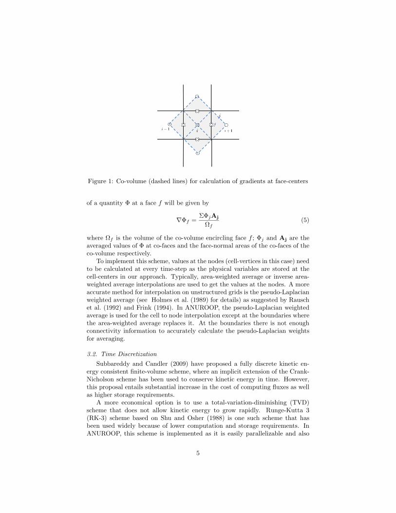
Figure 1: Co-volume (dashed lines) for calculation of gradients at face-centers

of a quantity Φ at a face f will be given by

∇Φf =ΣΦjAj

Ωf(5)

where Ωf is the volume of the co-volume encircling face f ; Φj and Aj are theaveraged values of Φ at co-faces and the face-normal areas of the co-faces of theco-volume respectively.

To implement this scheme, values at the nodes (cell-vertices in this case) needto be calculated at every time-step as the physical variables are stored at thecell-centers in our approach. Typically, area-weighted average or inverse area-weighted average interpolations are used to get the values at the nodes. A moreaccurate method for interpolation on unstructured grids is the pseudo-Laplacianweighted average (see Holmes et al. (1989) for details) as suggested by Rauschet al. (1992) and Frink (1994). In ANUROOP, the pseudo-Laplacian weightedaverage is used for the cell to node interpolation except at the boundaries wherethe area-weighted average replaces it. At the boundaries there is not enoughconnectivity information to accurately calculate the pseudo-Laplacian weightsfor averaging.

3.2. Time Discretization

Subbareddy and Candler (2009) have proposed a fully discrete kinetic en-ergy consistent finite-volume scheme, where an implicit extension of the Crank-Nicholson scheme has been used to conserve kinetic energy in time. However,this proposal entails substantial increase in the cost of computing fluxes as wellas higher storage requirements.

A more economical option is to use a total-variation-diminishing (TVD)scheme that does not allow kinetic energy to grow rapidly. Runge-Kutta 3(RK-3) scheme based on Shu and Osher (1988) is one such scheme that hasbeen used widely because of lower computation and storage requirements. InANUROOP, this scheme is implemented as it is easily parallelizable and also

5

more scalable (Allaneau and Jameson, 2009), and hence is suitable for DNSstudies. The implementation of RK-3 is as follows: For the equation

dU

dt+R(U) = 0

RK-3 takes

U (1) = U (n) −∆t R(U (n))

U (2) =3

4U (n) +

1

4U (1) − 1

4∆t R(U (1))

U (n+1) =1

3U (n) +

2

3U (1) − 2

3∆t R(U (2))

Calculation of Time Step

In ANUROOP, the maximum allowable time step is calculated using theCourant-Friedrichs-Lewy (CFL) condition. This condition ensures that the flowon the stencil of a grid respects the physics. For the 1D Euler equations, theCFL condition for time step is given by

∆t = σ∆x

|Λ|

where ∆x/|Λ| is the time needed for information to propagate on a grid of size∆x with velocity Λ, and σ is a positive coefficient, known as the CFL number.For Euler flows, Λ corresponds to the maximum eigen value in the convectiveflux Jacobian. For viscous flows, the spectral radius of the viscous flux Jacobianneeds to be included in the calculation of maximum ∆t as the flow in theboundary layer can severely restrict the maximum allowable time-step.

For 3D viscous calculations in ANUROOP on unstructured grids, the time-step computation follows the method suggested by Blazek (2005),

∆ti = σΩi

(Λinv + C Λv)i(6)

Here Λinv and Λv represent a sum of Euler and viscous spectral radii of all thefaces over all control volumes, and are given by:

(Λinv)i =

NF∑J=1

(|v · n|+ c) ∆SJ

(Λv)i =1

Ωi

NF∑J=1

[max

(4

3ρ,γ

ρ

)(µ

Pr

)(∆SJ)2

]Here v · n and c are the normal velocity and speed of sound on face J of cell irespectively; ∆SJ and Ωi are geometrical parameters representing area of faceJ and volume of cell i containing all such faces.

The constant C that multiplies the viscous spectral radius Λv is taken as 4(recommended for central schemes in Blazek (2005)), and the CFL number iskept below 1 for the time-stepping through out the computation.

6

4. Boundary Conditions

Inlet, outlet, wall and periodic boundary conditions, which are needed tosimulate the flow between consecutive blades, are implemented in ANUROOP.The values of primitive variables at the boundary are updated every time-stepusing the boundary conditions. All the boundary conditions are imposed byadding ghost cells. For periodic boundary conditions, the values at the firstinterior cells of the first boundary are copied to corresponding ghost cells in theother periodic boundary and vice versa.

For wall, inlet and outlet, the details of the boundary conditions implementedin ANUROOP are given below.

4.1. Wall Boundary Condition

For the wall a mirror boundary condition has been used, where the variablesin the interior cells next to the boundary are mirrored appropriately to corre-sponding ghost cells and an average is taken to get the value at the wall face.For a no-slip stationary isothermal wall, the ghost values are as follows:

ug = −uivg = −viwg = −wiTg = 2× Tw − Ti

where subscript i and g stand for interior and ghost cells respectively. Tw isthe imposed wall temperature. The density is obtained using the continuityequation.

4.2. Inlet/Outlet Boundary Conditions

The treatment of flow at the inlet and outlet is critical, since in the sim-ulation an infinite flow domain is restricted to a finite computational domain.An improper boundary condition may lead to unphysical oscillations near theboundary, which with progress in time may either lead to blow up of the codeor give spurious results. It is necessary to avoid the reflection of the outgoingwaves (from the computational domain) to ensure smooth inflow/outflow. To dothis, primitive variables at the boundary are extrapolated using characteristicsvariables (known as Riemann invariants), as given in Hirsch (1988).

The Riemann invariants are calculated based on the values at the interiorcells of the boundaries or the far-field values, depending on whether the char-acteristics point inwards or outwards.

For 3D Euler equations there are 5 eigen values (characteristics) of the Ja-cobian matrix, given by

λ1 = u⊥ + c (7a)

λ2,3,4 = u⊥ (7b)

λ5 = u⊥ − c (7c)

7

where the subscript ⊥ indicates the velocity normal to the boundary face, givenby v · n.

These eigen values determine whether the wave is entering or leaving the do-main. At the subsonic inlet (−1 ≤M⊥ < 0; u⊥ < 0, c > 0, u⊥ < c), there is oneright running wave (u⊥+c > 0) and two left-running waves (u⊥ < 0, u⊥−c < 0).At the subsonic outlet (0 ≥ M⊥ < 1; u⊥ > 0, c > 0, u⊥ < c), there are tworight running waves (u⊥ > 0, u⊥+c > 0) and one left-running wave (u⊥−c < 0).The invariants corresponding to the right running wave are calculated based onthe values at the interior cells and those corresponding to the left-running waveare calculated based on far-field values, as given below.

Subsonic inflow boundary

ψ1 ≡ ψ1i =2ciγ − 1

+ u⊥i (8a)

ψ2 ≡ ψ2∞ =p∞ργ∞

(8b)

ψ3 ≡ ψ3∞ =2c∞γ − 1

− u⊥∞ (8c)

Subsonic outflow boundary

ψ1 ≡ ψ1i =2ciγ − 1

+ u⊥i (9a)

ψ2 ≡ ψ2i =piργi

(9b)

ψ3 ≡ ψ3∞ =2c∞γ − 1

− u⊥∞ (9c)

After the invariants are known, the values at the boundary face are thus extrap-olated as

u⊥bf =ψ1 + ψ3

2

cbf =

(γ − 1

4

)(ψ1 − ψ3)

ρbf =

(a2fγψ2

) 1γ−1

pbf =ρfa

2f

γ

u⊥bf is then again back-transformed to get all 3 components of velocity at theboundary.

For the simulations with inflow turbulence, the turbulent fluctuations aresuperimposed on the mean value of the velocities as obtained from the boundarycondition.

8

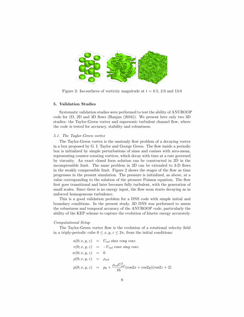
Figure 2: Iso-surfaces of vorticity magnitude at t = 0.5, 2.0 and 13.0

5. Validation Studies

Systematic validation studies were performed to test the ability of ANUROOPcode for 1D, 2D and 3D flows (Ranjan (2016)). We present here only two 3Dstudies: the Taylor-Green vortex and supersonic turbulent channel flow, wherethe code is tested for accuracy, stability and robustness.

5.1. The Taylor-Green vortex

The Taylor-Green vortex is the unsteady flow problem of a decaying vortexin a box proposed by G. I. Taylor and George Green. The flow inside a periodicbox is initialized by simple perturbations of sines and cosines with zero-mean,representing counter-rotating vortices, which decay with time at a rate governedby viscosity. An exact closed form solution can be constructed in 2D in theincompressible limit. The same problem in 2D can be extended to 3-D flowsin the weakly compressible limit. Figure 2 shows the stages of the flow as timeprogresses in the present simulation. The pressure is initialized, as above, at avalue corresponding to the solution of the pressure Poisson equation. The flowfirst goes transitional and later becomes fully turbulent, with the generation ofsmall scales. Since there is no energy input, the flow soon starts decaying as inunforced homogeneous turbulence.

This is a good validation problem for a DNS code with simple initial andboundary conditions. In the present study, 3D DNS was performed to assessthe robustness and temporal accuracy of the ANUROOP code, particularly theability of the KEP scheme to capture the evolution of kinetic energy accurately.

Computational Setup

The Taylor-Green vortex flow is the evolution of a rotational velocity fieldin a triply-periodic cube 0 ≤ x, y, z ≤ 2π, from the initial conditions:

u(0;x, y, z) = Uref sinx cosy cosz

v(0;x, y, z) = −Uref cosx siny cosz

w(0;x, y, z) = 0

ρ(0;x, y, z) = ρref

p(0;x, y, z) = p0 +ρrefU

2ref

16(cos2x+ cos2y)(cos2z + 2)

9

0 5 10 15 200

0.005

0.01

t

−dk/

dt

(a)

(b)

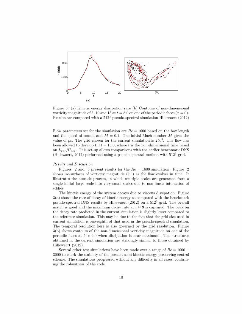
Figure 3: (a) Kinetic energy dissipation rate (b) Contours of non-dimensionalvorticity magnitude of 5, 10 and 15 at t = 8.0 on one of the periodic faces (x = 0).Results are compared with a 5123 pseudo-spectral simulation Hillewaert (2012)

Flow parameters set for the simulation are Re = 1600 based on the box lengthand the speed of sound, and M = 0.1. The initial Mach number M gives thevalue of p0. The grid chosen for the current simulation is 2563. The flow hasbeen allowed to develop till t = 13.0, where t is the non-dimensional time basedon Lref/Uref . This set-up allows comparisons with the earlier benchmark DNS(Hillewaert, 2012) performed using a psuedo-spectral method with 5123 grid.

Results and Discussion

Figures 2 and 3 present results for the Re = 1600 simulation. Figure 2shows iso-surfaces of vorticity magnitude (|ω|) as the flow evolves in time. Itillustrates the cascade process, in which multiple scales are generated from asingle initial large scale into very small scales due to non-linear interaction ofeddies.

The kinetic energy of the system decays due to viscous dissipation. Figure3(a) shows the rate of decay of kinetic energy as compared with the benchmarkpseudo-spectral DNS results by Hillewaert (2012) on a 5123 grid. The overallmatch is good and the maximum decay rate at t ≈ 9 is captured. The peak onthe decay rate predicted in the current simulation is slightly lower compared tothe reference simulation. This may be due to the fact that the grid size used incurrent simulation is one-eighth of that used in the pseudo-spectral simulation.The temporal resolution here is also governed by the grid resolution. Figure3(b) shows contours of the non-dimensional vorticity magnitude on one of theperiodic faces at t ≈ 9.0 when dissipation is near maximum. The structuresobtained in the current simulation are strikingly similar to those obtained byHillewaert (2012).

Several other test simulations have been made over a range of Re = 1000−3000 to check the stability of the present semi kinetic-energy preserving centralscheme. The simulations progressed without any difficulty in all cases, confirm-ing the robustness of the code.

10

5.2. Supersonic Turbulent Channel Flow

DNS of compressible channnel flow has been performed to test the ANUROOPcode against wall-bounded flows at finite Mach number. Past studies by Cole-man et al. (1995) for an isothermal supersonic channel flow offer a good case forvalidation of the present code. Two plates separated by a width of 2H constitutethe channel in which the fluid flows. The flow is statistically homogeneous in thestreamwise (x) as well as spanwise(z) directions, and is driven by a body-forcethat keeps the mass-flux constant.

Problem Formulation

The main parameters governing the flow are Mach number and Reynoldsnumber. Of the various cases described in Coleman et al. (1995), the one chosenhere for the validation is atM = 1.5 andRe = 3000 (based on centerline velocity,viscosity at wall temperature, and channel half-height H). Prandtl number Pris kept constant at 0.7 throughout the flow and the viscosity of the fluid variesaccording to the power law µ ∝ (T/Tw)0.7, where Tw is the prescribed (constant)wall temperature.

Body-force terms have been added as sources in the momentum and energyequations in Eqn. 1. The body force is varied with time to keep stream-wisemass-flux constant. Thus, the change in body-force after every iteration is givenby

∆B =(∫ρudydz)n − (

∫ρudydz)n−1

(∫ρdydz)n

Geometry and Grid

The sides of the computational domain are Lx = 2π, Ly = 2, Lz = 4π/3.There are 100 grid points chosen in each direction to make the grid. The gridis uniform in streamwise (x) and spanwise (z) directions but stretching is usedalong wall-normal direction y to obtain a sufficiently fine grid to capture thenear-wall flow. The stretching is done using the hyperbolic tangent function, asfollows:

yj =tanh[c(2(j − 1)/(ny − 1)− 1]

tanh(c)

where ny is the total number of grid-points in the y-direction and c is a constanttaken as 1.7 (as in Subbareddy and Candler (2009)). The range of y spans −1to +1 with y = 0 at the centerline of the channel.

The simulation has been initialized with a parabolic laminar velocity profilesuperimposed with white noise (with zero mean) perturbations.

Results and Discussion

Instantaneous quantities have been time- and span-averaged to get the meanvalues. Favre-averaging that accounts for density variations is used to obtainthe Favre mean, defined as follows:

φ =〈ρφ〉〈ρ〉

11

−1 −0.5 0 0.5 10

0.2

0.4

0.6

0.8

1

1.2

1.4

y

〈u〉

(a)

10−1 100 101 102 1030

5

10

15

20

25

y+

⟨u⟩+

⟨u⟩+Anuroop

⟨u⟩+Coleman

⟨u⟩+V D

⟨u⟩+ = 1/κ ln y+ + B

⟨u⟩+ = y+

( )

(b)

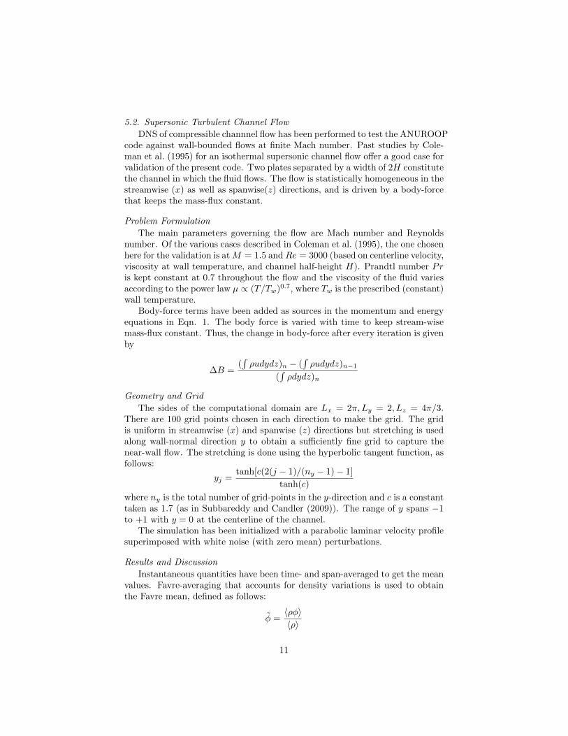
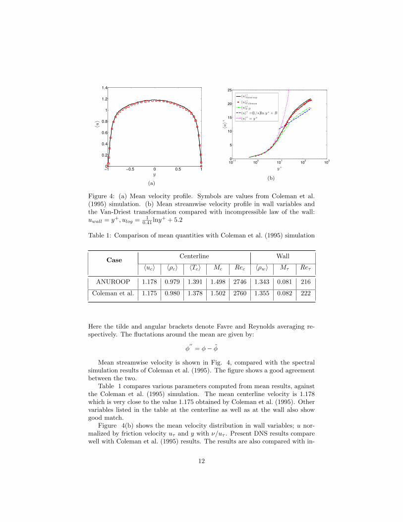
Figure 4: (a) Mean velocity profile. Symbols are values from Coleman et al.(1995) simulation. (b) Mean streamwise velocity profile in wall variables andthe Van-Driest transformation compared with incompressible law of the wall:uwall = y+, ulog = 1

0.41 lny+ + 5.2

Table 1: Comparison of mean quantities with Coleman et al. (1995) simulation

CaseCenterline Wall

〈uc〉 〈ρc〉 〈Tc〉 Mc Rec 〈ρw〉 Mτ Reτ

ANUROOP 1.178 0.979 1.391 1.498 2746 1.343 0.081 216

Coleman et al. 1.175 0.980 1.378 1.502 2760 1.355 0.082 222

Here the tilde and angular brackets denote Favre and Reynolds averaging re-spectively. The fluctations around the mean are given by:

φ′′

= φ− φ

Mean streamwise velocity is shown in Fig. 4, compared with the spectralsimulation results of Coleman et al. (1995). The figure shows a good agreementbetween the two.

Table 1 compares various parameters computed from mean results, againstthe Coleman et al. (1995) simulation. The mean centerline velocity is 1.178which is very close to the value 1.175 obtained by Coleman et al. (1995). Othervariables listed in the table at the centerline as well as at the wall also showgood match.

Figure 4(b) shows the mean velocity distribution in wall variables; u nor-malized by friction velocity uτ and y with ν/uτ . Present DNS results comparewell with Coleman et al. (1995) results. The results are also compared with in-

12

compressible law of the wall for turbulent flows, which states that in the viscoussublayer region (y+ < 10)

uwall = y+ (10)

and in the log-law region (10 < y+ < 100)

〈u〉+ =1

κln y+ +B (11)

where κ = 0.41 is the Von Karman constant and B = 5.2 is the intercept atlny+ = 0.

In both ANUROOP and Coleman et al. (1995) simulations, 〈u〉+ agrees wellwith the law of the wall in the viscous sublayer, however it is far away in thelog-law region. For high mach number flows, where density variation is veryhigh, variables are not expected to follow the incompressible laws. However adensity-weighted transformation of mean velocity (also known as the Van Driesttransformation), can be used to enable this comparison. This transformation isgiven as:

〈u〉+V D =

∫ 〈u〉+0

(〈ρ〉ρw

) 12

d〈u〉+ (12)

This transformed velocity is expected to satisfy the incompressible log law(Bradshaw (1977))

〈u〉+V D =1

κln y+ +B (13)

The above law is also plotted in Fig. 4(b) and it can be noted that thistransformation brings the profile closer to the incompressible log-law; howeverin the overlap region (5 < y+ < 10) the agreement becomes worse. Wei andPollard (2011) argue that a power law is slightly better and less dependent onMach number than the log-law in this region.

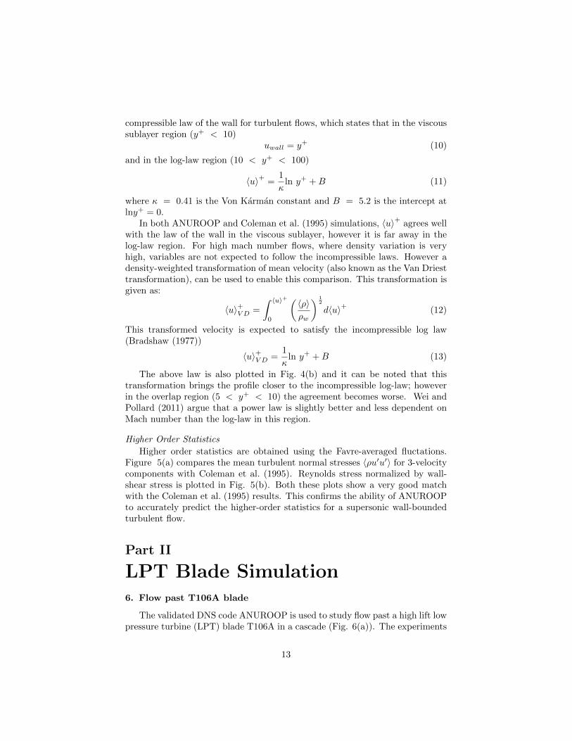
Higher Order Statistics

Higher order statistics are obtained using the Favre-averaged fluctations.Figure 5(a) compares the mean turbulent normal stresses 〈ρu′u′〉 for 3-velocitycomponents with Coleman et al. (1995). Reynolds stress normalized by wall-shear stress is plotted in Fig. 5(b). Both these plots show a very good matchwith the Coleman et al. (1995) results. This confirms the ability of ANUROOPto accurately predict the higher-order statistics for a supersonic wall-boundedturbulent flow.

Part II

LPT Blade Simulation6. Flow past T106A blade

The validated DNS code ANUROOP is used to study flow past a high lift lowpressure turbine (LPT) blade T106A in a cascade (Fig. 6(a)). The experiments

13

−1 −0.5 0 0.5 1

0

0.01

0.02

0.03

y

〈ρu

′′ iu

′′ j〉/〈ρ〉

u′ ′u

′ ′

v′ ′v

′ ′

w′ ′w

′ ′

(a)

−1 −0.5 0 0.5 1

−0.5

0

0.5

y

⟨ρu

′ v′ ⟩/

⟨τw⟩

(b)

Figure 5: (a) Turbulent normal stresses (〈ρu′u′〉). (b)Reynolds stress normal-ized by the wall-shear stress. Symbols are values from Coleman et al. (1995)simulation

reported by Stadtmuller (2002) provide the flow parameters used in the presentDNS study. The tests were performed in the High Speed Cascade Wind Tunnelof the Universitat der Bundeswehr, Munchen, Germany, with the purpose ofproviding test data at low Re suitable for DNS studies. The surface pressuremeasurements and hot-film traces clearly indicate a separation bubble near thetrailing edge (TE) of the suction side; however it is not clear whether the bubblereattaches. The report does not mention the presence of any separation bubblenear the leading edge (LE) as found in many DNS studies at low resolution(Kalitzin et al. (2003); Wissink (2003); Wissink et al. (2006); Michelassi et al.(2002); Ranjan et al. (2015)).

All the measurements needed for the flow condition are taken in the outflowplane of the cascade, and isentropic relations are used to get the upstreamconditions for the computational studies. We use Re = 51, 831 based on the inletvelocity and the axial chord length (lax) as used in most of the DNS studies in thepast for this experiment. Stadtmuller (2002) mentions considerable uncertaintyover the exact inlet angle to be chosen for the computational study, due tothe presence of the wake generator ahead of the cascade. Based on RANSsimulations and 3D hot wire measurements, Stadtmuller (2002) has estimatedthe real inlet flow angle as 45.5. This value is used for the present DNS study.

Further, the experiments were performed in a steady upstream flow (distur-bance free environment) as well as with upstream wakes created by a moving-barwake-generator. We have performed simulations without free-stream turbulenceas well as with turbulent intensities of 5% and 10%. However, the present dis-cussion confines itself to computational study with steady-state measurements(without any free-stream turbulence or wake) as the focus is on a detailed bound-ary layer study with minimum uncertainties. Results with more complex inletconditions will appear in later studies.

14

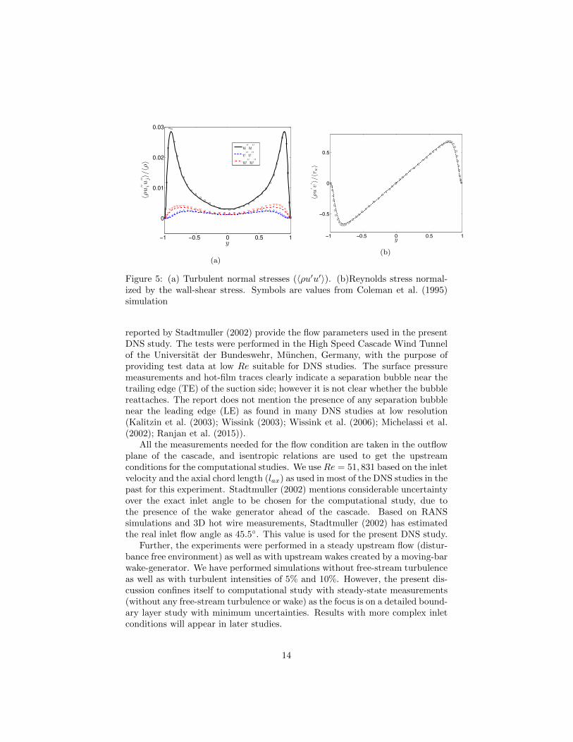
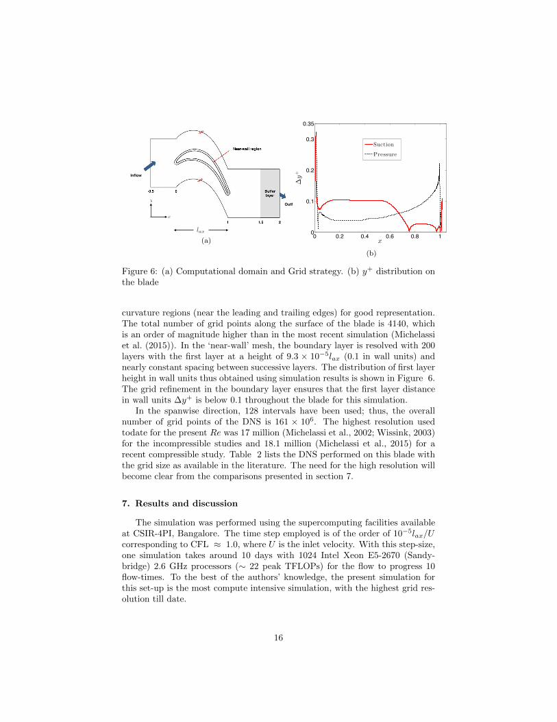
6.1. Computational domain and grid strategy

The computational domain, illustrated in Fig. 6, covers the flow around ablade with periodic boundary conditions that simulate the row of blades at topand bottom. The outflow plane is located at a distance of one axial chord laxdownstream of the TE, and the inflow plane is at a distance of half the axialchord upstream of the LE. The pitch between the blades is p = 0.9306 lax,and periodic boundary conditions are applied everywhere on the boundary inthe pitchwise y-direction as well as spanwise z-direction. A no-slip isothermalboundary condition is applied at the blade surface.

The elliptic scheme used in earlier work (Wu and Durbin (2001); Kalitzinet al. (2003); Wissink (2003); Wissink et al. (2006); Michelassi et al. (2002))offers little control over grid generation in the interior. Kalitzin et al. (2003)have reported a large number of skewed elements in the passage near the TEusing this scheme, due to the strong curvature and requirement of periodicityin the pitchwise direction. Their results near the LE also exhibit the effect ofsingularity in the forced H-mesh used in the study. Wissink (2003) has reportedthe effect of streamwise resolution on the accuracy with which the separationbubbles can be resolved. Garai et al. (2015) have reported oscillations in theirsimulations in the pressure distribution due to low-order geometry representa-tion of the blade profile. These oscillations become more prominent in the highcurvature regions.

Because of these observations and the present emphasis on the boundarylayer, greater control and flexibility on the grid in the boundary layer was soughton the following three aspects:

• Orthogonal mesh without any singularity near the blade wall

• Control on boundary layer grid with respect to the first grid-point nearthe wall and the ratio of heights of the successive layers

• Control on streamwise resolution without unduly increasing the overallgrid size

It is difficult to meet all these requirements in the elliptic mesh approach,especially because of the periodicity of the mesh elements in the pitchwise (y)direction. In our approach, the domain has been divided into two regions: ‘near-wall’ and ‘outer’ (Fig. 6). In the near-wall region, an orthogonal boundary layermesh is built by specifying the first grid point away from the wall, the successiveratio and the number of rows in the boundary layer. After the near-wall meshis ready, the outer region was filled with quadrilateral elements ensuring propermesh distribution along the rest of the edges of the domain. Periodicity isenforced in the pitchwise y-direction by exactly copying elements along theperiodic edges. It requires a few iterations to get the desirable mesh with noabrupt jump and of good quality. More than 50% of the total number of meshelements are confined in the near-wall region.

In the streamwise direction, the blade airfoil was divided into 3 parts onboth suction and pressure sides, and a very fine clustered grid is used in the high

15

lax

Outflow

Inflow

y

x

(a)0 0.2 0.4 0.6 0.8 10

0.1

0.2

0.3

0.35

x

∆y+

Suction

Pressure

(b)

Figure 6: (a) Computational domain and Grid strategy. (b) y+ distribution onthe blade

curvature regions (near the leading and trailing edges) for good representation.The total number of grid points along the surface of the blade is 4140, whichis an order of magnitude higher than in the most recent simulation (Michelassiet al. (2015)). In the ‘near-wall’ mesh, the boundary layer is resolved with 200layers with the first layer at a height of 9.3 × 10−5lax (0.1 in wall units) andnearly constant spacing between successive layers. The distribution of first layerheight in wall units thus obtained using simulation results is shown in Figure 6.The grid refinement in the boundary layer ensures that the first layer distancein wall units ∆y+ is below 0.1 throughout the blade for this simulation.

In the spanwise direction, 128 intervals have been used; thus, the overallnumber of grid points of the DNS is 161 × 106. The highest resolution usedtodate for the present Re was 17 million (Michelassi et al., 2002; Wissink, 2003)for the incompressible studies and 18.1 million (Michelassi et al., 2015) for arecent compressible study. Table 2 lists the DNS performed on this blade withthe grid size as available in the literature. The need for the high resolution willbecome clear from the comparisons presented in section 7.

7. Results and discussion

The simulation was performed using the supercomputing facilities availableat CSIR-4PI, Bangalore. The time step employed is of the order of 10−5lax/Ucorresponding to CFL ≈ 1.0, where U is the inlet velocity. With this step-size,one simulation takes around 10 days with 1024 Intel Xeon E5-2670 (Sandy-bridge) 2.6 GHz processors (∼ 22 peak TFLOPs) for the flow to progress 10flow-times. To the best of the authors’ knowledge, the present simulation forthis set-up is the most compute intensive simulation, with the highest grid res-olution till date.

16

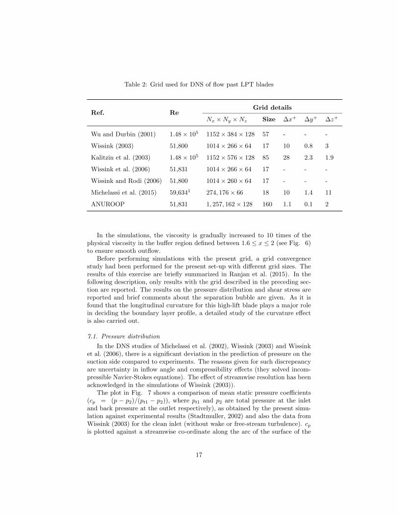
Table 2: Grid used for DNS of flow past LPT blades

Ref. ReGrid details

Nx ×Ny ×Nz Size ∆x+ ∆y+ ∆z+

Wu and Durbin (2001) 1.48× 105 1152× 384× 128 57 - - -

Wissink (2003) 51,800 1014× 266× 64 17 10 0.8 3

Kalitzin et al. (2003) 1.48× 105 1152× 576× 128 85 28 2.3 1.9

Wissink et al. (2006) 51,831 1014× 266× 64 17 - - -

Wissink and Rodi (2006) 51,800 1014× 260× 64 17 - - -

Michelassi et al. (2015) 59,6341 274, 176× 66 18 10 1.4 11

ANUROOP 51,831 1, 257, 162× 128 160 1.1 0.1 2

In the simulations, the viscosity is gradually increased to 10 times of thephysical viscosity in the buffer region defined between 1.6 ≤ x ≤ 2 (see Fig. 6)to ensure smooth outflow.

Before performing simulations with the present grid, a grid convergencestudy had been performed for the present set-up with different grid sizes. Theresults of this exercise are briefly summarized in Ranjan et al. (2015). In thefollowing description, only results with the grid described in the preceding sec-tion are reported. The results on the pressure distribution and shear stress arereported and brief comments about the separation bubble are given. As it isfound that the longitudinal curvature for this high-lift blade plays a major rolein deciding the boundary layer profile, a detailed study of the curvature effectis also carried out.

7.1. Pressure distribution

In the DNS studies of Michelassi et al. (2002), Wissink (2003) and Wissinket al. (2006), there is a significant deviation in the prediction of pressure on thesuction side compared to experiments. The reasons given for such discrepeancyare uncertainty in inflow angle and compressibility effects (they solved incom-pressible Navier-Stokes equations). The effect of streamwise resolution has beenacknowledged in the simulations of Wissink (2003)).

The plot in Fig. 7 shows a comparison of mean static pressure coefficients(cp = (p − p2)/(pt1 − p2)), where pt1 and p2 are total pressure at the inletand back pressure at the outlet respectively), as obtained by the present simu-lation against experimental results (Stadtmuller, 2002) and also the data fromWissink (2003) for the clean inlet (without wake or free-stream turbulence). cpis plotted against a streamwise co-ordinate along the arc of the surface of the

17

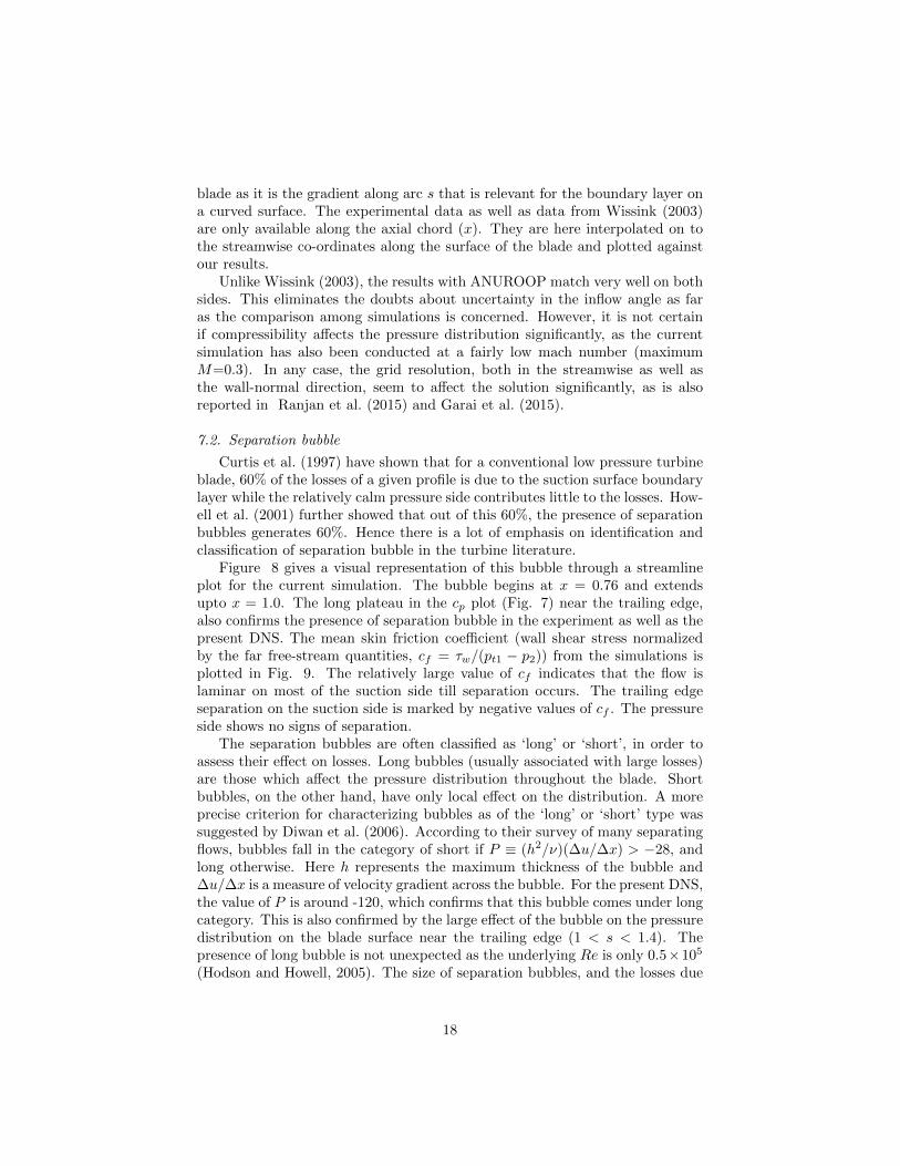
blade as it is the gradient along arc s that is relevant for the boundary layer ona curved surface. The experimental data as well as data from Wissink (2003)are only available along the axial chord (x). They are here interpolated on tothe streamwise co-ordinates along the surface of the blade and plotted againstour results.

Unlike Wissink (2003), the results with ANUROOP match very well on bothsides. This eliminates the doubts about uncertainty in the inflow angle as faras the comparison among simulations is concerned. However, it is not certainif compressibility affects the pressure distribution significantly, as the currentsimulation has also been conducted at a fairly low mach number (maximumM=0.3). In any case, the grid resolution, both in the streamwise as well asthe wall-normal direction, seem to affect the solution significantly, as is alsoreported in Ranjan et al. (2015) and Garai et al. (2015).

7.2. Separation bubble

Curtis et al. (1997) have shown that for a conventional low pressure turbineblade, 60% of the losses of a given profile is due to the suction surface boundarylayer while the relatively calm pressure side contributes little to the losses. How-ell et al. (2001) further showed that out of this 60%, the presence of separationbubbles generates 60%. Hence there is a lot of emphasis on identification andclassification of separation bubble in the turbine literature.

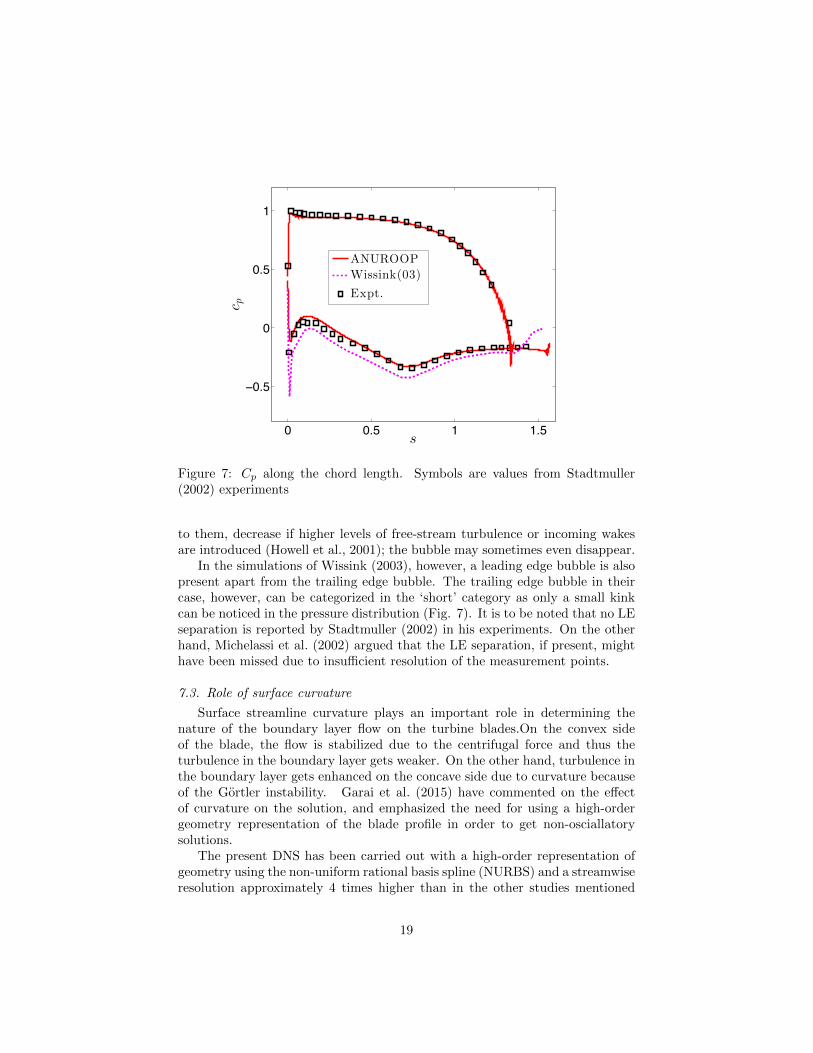
Figure 8 gives a visual representation of this bubble through a streamlineplot for the current simulation. The bubble begins at x = 0.76 and extendsupto x = 1.0. The long plateau in the cp plot (Fig. 7) near the trailing edge,also confirms the presence of separation bubble in the experiment as well as thepresent DNS. The mean skin friction coefficient (wall shear stress normalizedby the far free-stream quantities, cf = τw/(pt1 − p2)) from the simulations isplotted in Fig. 9. The relatively large value of cf indicates that the flow islaminar on most of the suction side till separation occurs. The trailing edgeseparation on the suction side is marked by negative values of cf . The pressureside shows no signs of separation.

The separation bubbles are often classified as ‘long’ or ‘short’, in order toassess their effect on losses. Long bubbles (usually associated with large losses)are those which affect the pressure distribution throughout the blade. Shortbubbles, on the other hand, have only local effect on the distribution. A moreprecise criterion for characterizing bubbles as of the ‘long’ or ‘short’ type wassuggested by Diwan et al. (2006). According to their survey of many separatingflows, bubbles fall in the category of short if P ≡ (h2/ν)(∆u/∆x) > −28, andlong otherwise. Here h represents the maximum thickness of the bubble and∆u/∆x is a measure of velocity gradient across the bubble. For the present DNS,the value of P is around -120, which confirms that this bubble comes under longcategory. This is also confirmed by the large effect of the bubble on the pressuredistribution on the blade surface near the trailing edge (1 < s < 1.4). Thepresence of long bubble is not unexpected as the underlying Re is only 0.5×105

(Hodson and Howell, 2005). The size of separation bubbles, and the losses due

18

0 0.5 1 1.5

−0.5

0

0.5

1

s

c p

ANUROOPWissink(03)

Expt.

Figure 7: Cp along the chord length. Symbols are values from Stadtmuller(2002) experiments

to them, decrease if higher levels of free-stream turbulence or incoming wakesare introduced (Howell et al., 2001); the bubble may sometimes even disappear.

In the simulations of Wissink (2003), however, a leading edge bubble is alsopresent apart from the trailing edge bubble. The trailing edge bubble in theircase, however, can be categorized in the ‘short’ category as only a small kinkcan be noticed in the pressure distribution (Fig. 7). It is to be noted that no LEseparation is reported by Stadtmuller (2002) in his experiments. On the otherhand, Michelassi et al. (2002) argued that the LE separation, if present, mighthave been missed due to insufficient resolution of the measurement points.

7.3. Role of surface curvature

Surface streamline curvature plays an important role in determining thenature of the boundary layer flow on the turbine blades.On the convex sideof the blade, the flow is stabilized due to the centrifugal force and thus theturbulence in the boundary layer gets weaker. On the other hand, turbulence inthe boundary layer gets enhanced on the concave side due to curvature becauseof the Gortler instability. Garai et al. (2015) have commented on the effectof curvature on the solution, and emphasized the need for using a high-ordergeometry representation of the blade profile in order to get non-osciallatorysolutions.

The present DNS has been carried out with a high-order representation ofgeometry using the non-uniform rational basis spline (NURBS) and a streamwiseresolution approximately 4 times higher than in the other studies mentioned

19

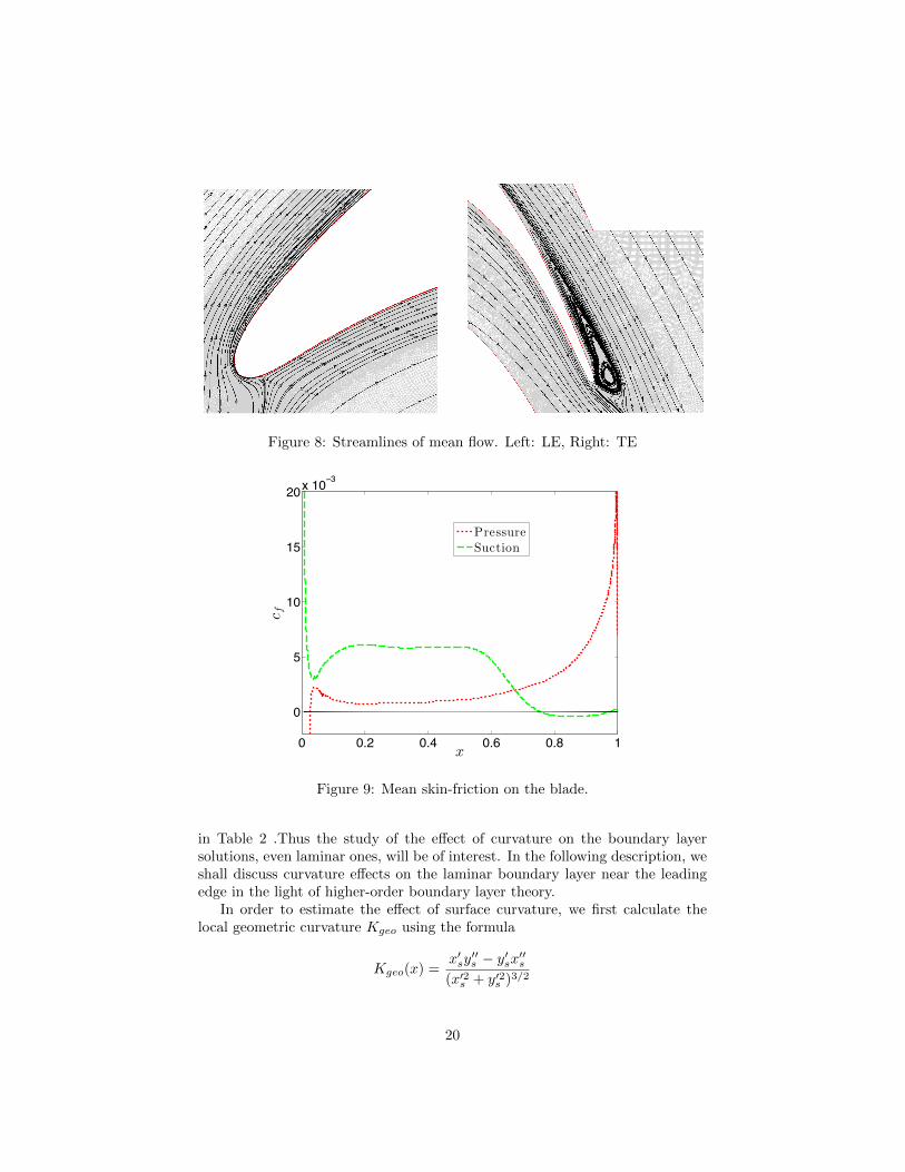
Figure 8: Streamlines of mean flow. Left: LE, Right: TE

0 0.2 0.4 0.6 0.8 1

0

5

10

15

20x 10−3

x

c f

PressureSuction

Figure 9: Mean skin-friction on the blade.

in Table 2 .Thus the study of the effect of curvature on the boundary layersolutions, even laminar ones, will be of interest. In the following description, weshall discuss curvature effects on the laminar boundary layer near the leadingedge in the light of higher-order boundary layer theory.

In order to estimate the effect of surface curvature, we first calculate thelocal geometric curvature Kgeo using the formula

Kgeo(x) =x′sy′′s − y′sx′′s

(x′2s + y′2s )3/2

20

0 0.02 0.04 0.06 0.080

50

100

150

s

K

Kg e o

K (Eq. 15(b))

(a)

0

40

80

120

x

K

0.01 0.02 0.03 0.04

0

0.02

0.04

0.06

y

(b)

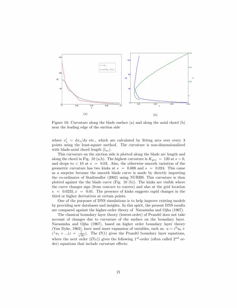
Figure 10: Curvature along the blade surface (a) and along the axial chord (b)near the leading edge of the suction side

where x′s = dxs/ds etc., which are calculated by fitting arcs over every 3points using the least-square method. The curvature is non-dimensionalizedwith blade-axial chord length (lax).

This curvature on the suction side is plotted along the blade arc length andalong the chord in Fig. 10 (a,b). The highest curvature is Kgeo = 120 at s ∼ 0,and drops to < 10 at s = 0.03. Also, the otherwise smooth variation of thegeometric curvature has two kinks at s = 0.008 and s = 0.024. This cameas a surprise because the smooth blade curve is made by directly importingthe co-ordinates of Stadtmuller (2002) using NURBS. This curvature is thenplotted against the the blade curve (Fig. 10 (b)). The kinks are visible wherethe curve changes sign (from concave to convex) and also at the grid locations = 0.0235, x = 0.01. The presence of kinks suggests rapid changes in thethird or higher derivatives at certain points.

One of the purposes of DNS simulations is to help improve existing modelsby providing new databases and insights. In this spirit, the present DNS resultsare compared against the higher-order theory of Narasimha and Ojha (1967).

The classical boundary layer theory (lowest-order) of Prandtl does not takeaccount of changes due to curvature of the surface on the boundary layer.Narasimha and Ojha (1967), based on higher order boundary layer theory(Van Dyke, 1962), have used inner expansion of variables, such as: u = ε0u0 +ε1u1 + ...(ε = 1√

Re). The O(1) gives the Prandtl boundary layer equations,

where the next order (O(ε)) gives the following 1st-order (often called 2nd or-der) equations that include curvature effects:

21

∂u1∂x

+∂

∂y(v1 +K y u0) = 0 (14a)

u0∂u1∂x

+ v0∂u1∂y

+ u1∂u0∂x

+ v1∂u0∂y

=− ∂

∂x

K

∫ y

0

u20 dy +K

∫ ∞0

(U20s − u20) dy

+∂2u1∂y2

+K

y(u0∂u0∂x

+∂p0∂x

)+∂u0∂y− u0v0

(14b)

with the boundary conditions

u1 = v1 = 0, at y = 0, (15a)

and u1 = −K y U0s, as y →∞. (15b)

where subscripts 0 and 1 indicate solutions due to Prandtl’s boundary layertheory, and the curvature corrections respectively; K = K(s) is the curvatureof the blade and U0s = U0(X, 0) is the surface speed from the outer solutionas illustrated in Fig. 11(b).

Narasimha and Ojha (1967) have also given a Falkner-Skan like similaritysolution for these equations under special conditions, where the velocity variesas a power law with distance as U0s = Csm. Hence in the transformed co-ordinate (η) system, the final solution can be written as f = f0 + εf1. Here f0is the solution of the usual Falkner-Skan similarity equations,

f′′′

0 + f0f′′

0 = β(f′20 − 1) (16)

where β =2m

m+ 1, and the equation for first-order variable f1 is given as:

f′′′

1 + f0f′′

1 − 2 βf′

0f′

1 + f′′

0 f1 = κ

[f′′

0 (ηf0 − 1)− f0f′′

0

− βη(f

′20 − 1)− 2

1 + β(f′′

0 + f0f′

0 + βη +A)

](17)

where

K = κ

[C(m+ 1)

2

] 12

s12 (m−1) (18)

A ≡ limη→∞

(η − f0) (19)

The boundary conditions in Equations 15 in similarity variables become

f1(0) = 0 = f′

1(0) (20a)

f′

1(η) ≈ −κ η as η →∞ (20b)

22

0 0.02 0.04 0.06 0.08

1.4

1.6

1.8

2

s

U0s

m = 0 .1656

m = −0 .1679

(a)

0 0.2 0.4 0.6 0.8 10

5

10

u/U0S

η

s = 0.057, K = 3.8

K δ ⋆0 = 0.0179, κϵ = 0.01

DNS

f ′0(η) + ϵf ′

1(η)

f ′0(η)

(b)

Figure 11: (a) Surface velocity fit for favourable and adverse pressure gradient(FPG and APG) regions in the locality of high curvature. These fits were used tocalculate Falkner-Skan as well 1st-order solutions (b) Curvature effects: Prandtlvs Higher Order at s = 0.057. DNS results are also plotted.

Here the primes denote differentiation with respect to the transformed co-ordinate η. The overall velocity distribution, hence, can be given by u/U0S =f ′0 + κε(f ′1/κ).

In the present work, both equations 16 and 17 were solved sequentially usingthe shooting method. The Falkner-Skan exponent m was obtained using a localfit for the velocity as shown in Fig. 11(a). The effect of curvature can beseen in Fig. 11(b) where the velocity profiles with and without curvatureeffects are compared along with the DNS results for K = 3.8 (s = 0.057 on thesuction side). The corresponding Kδ?0 (or equivalently κε), which determinesthe applicability of 1st-order theory, is 0.0179 (or 0.01), where δ?0 is the boundarylayer thickness corresponding to Falkner-Skan solution. The Prandtl boundarylayer theory in the figure, shows a significant departure from the DNS solutions,while the 1st-order theory shows a very good match with the DNS results.

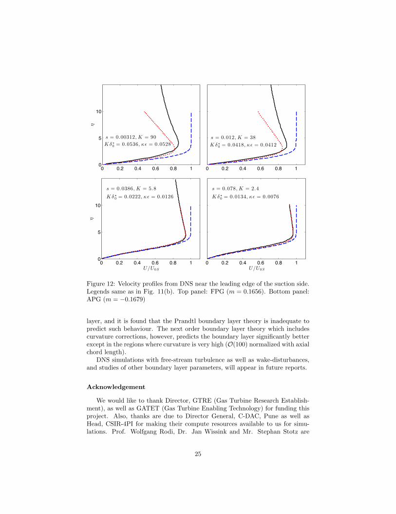
One can determine the value of Kδ?0 at which Equation 17 fails or separationis suspected. In Fig. 12 we present solutions at four locations. In the top panel,boundary layer profiles in the vicinity of the leading edge are shown, where thepressure gradient is favourable but curvature K is very high (O(100)). Theeffect of high surface curvature can be noticed in the ‘curved’ boundary layerprofiles as the solutions obtained by 1st-order theory in this region are found tobe not adequate. The region of overlap of both the plots in the outer solutionis very small, and one may require even higher order theory in order to predictthe boundary layer.

In the bottom panel, results are shown for two stations further downstream,where the pressure gradient is adverse but the curvature is relatively small[O(10)]. The effect of high surface curvature is weaker in these regions, and 1st-

23

order theory seems to be adequate to predict the boundary layer parameters.Similar observations are valid for all stations beyond s ≈ 0.0278 (Kδ?0 = 0.0353),where the curvatures obtained using the geometric formula as well as 1st-ordertheory are comparable (see Fig. 10(a)). 1st-order theory also predicts that theseparation in this region is possible at m = −0.1679 if Kδ?0 = 0.2624.

To the best of our knowledge, the present effort is the first assessment of thebounds of validity of the Prandtl boundary layer theory and the next higherorder approximation based on DNS results, especially for a problem of practicalimportance. Though the applicability of above results is restricted to laminarboundary layers, their importance lies in the fact that in many turbine blades theflow at the leading edge remains laminar and is prone to separation. Apart frompredicting boundary layer parameters, this theory can be used to predict theseparation for such flows. This is of importance to the designer as a separationbubble at the leading edge can trip the boundary layer towards turbulence.The applicability as well as accuracy of this theory can be further improvedby directly solving the governing equations instead of using fits to similaritysolutions.

The limitation of this theory is also mentioned above, where the predictionsfail in the vicinity of the leading edge for a high lift blade such as T106A. To getmore reliable solutions for such flow regimes, DNS may be the only approachwhich can be deemed adequate.

8. Conclusion

A new DNS code, ANUROOP, has been developed for simulating the flowpast a low pressure turbine blade. ANUROOP solves the compressible Navier-Stokes equations in the finite volume formulation and uses a flux-scheme thatrespects the conservation of evolution of kinetic energy. This code has been vali-dated for its accuracy and robustness for several benchmark problems includingTaylor-Green vortex and supersonic turbulent channel flow.

ANUROOP was then used to simulate flow past a high lift low-pressure tur-bine blade T106A at Re ≈ 52000 and an angle higher than the design incidence.No artificial inflow disturbance was used in the simulation. A highly resolvedboundary layer grid was used in all the three directions (streamwise, wall-normaland spanwise), which takes the total mesh count in the computational domainto around 160 million. The no. of mesh points used is approximately one orderof magnitude higher than that used in earlier studies for similar flow conditions.As a consequence pressure distribution predicted by the current simulation iscloser to the experimental values than in earlier simulations. This suggests thatthe earlier explanations of discrepancies in the pressure distributions, in partic-ular those attributing them to experimental uncertainties, may not be justified.

While the flow on the pressure side of the blade remains laminar, a ‘long’separation bubble forms in the aft region on the suction side disturbing the in-coming flow. The surface curvature of the blade significantly alters the boundary

24

0 0.2 0.4 0.6 0.8 10

5

10

s = 0.00312, K = 90

K δ ⋆0 = 0.0536, κϵ = 0.0528

η

0 0.2 0.4 0.6 0.8 1

s = 0.012, K = 38

K δ ⋆0 = 0.0418, κϵ = 0.0412

0 0.2 0.4 0.6 0.8 10

5

10

s = 0.0386, K = 5.8

K δ ⋆0 = 0.0222, κϵ = 0.0126

U/U0S

η

0 0.2 0.4 0.6 0.8 1

s = 0.078, K = 2.4

K δ ⋆0 = 0.0134, κϵ = 0.0076

U/U0S

Figure 12: Velocity profiles from DNS near the leading edge of the suction side.Legends same as in Fig. 11(b). Top panel: FPG (m = 0.1656). Bottom panel:APG (m = −0.1679)

layer, and it is found that the Prandtl boundary layer theory is inadequate topredict such behaviour. The next order boundary layer theory which includescurvature corrections, however, predicts the boundary layer significantly betterexcept in the regions where curvature is very high (O(100) normalized with axialchord length).

DNS simulations with free-stream turbulence as well as wake-disturbances,and studies of other boundary layer parameters, will appear in future reports.

Acknowledgement

We would like to thank Director, GTRE (Gas Turbine Research Establish-ment), as well as GATET (Gas Turbine Enabling Technology) for funding thisproject. Also, thanks are due to Director General, C-DAC, Pune as well asHead, CSIR-4PI for making their compute resources available to us for simu-lations. Prof. Wolfgang Rodi, Dr. Jan Wissink and Mr. Stephan Stotz are

25

gratefully acknowledged for providing crucial data pertaining to the study.

References

References

Allaneau Y, Jameson A. Direct numerical simulations of a two-dimensionalviscous flow in a shocktube using a kinetic energy preserving scheme. AIAApaper 2009 2009;3797.

Allaneau Y, Jameson A. Direct numerical simulations of plunging airfoils. In:48th AIAA Aerospace Sciences Meeting Including the New Horizons Forumand Aerospace Exposition, AIAA Paper. volume 728; 2010. .

Blazek J. Computational Fluid Dynamics: Principles and Applications:(Bookwith accompanying CD). Elsevier, 2005.

Bradshaw P. Compressible turbulent shear layers. Annual Review of FluidMechanics 1977;9(1):33–52.

Coleman GN, Kim J, Moser RD. A numerical study of turbulent supersonicisothermal-wall channel flow. Journal of Fluid Mechanics 1995;305:159–83.doi:10.1017/S0022112095004587.

Curtis E, Hodson H, Banieghbal M, Denton J, Howell R, Harvey N. Devel-opment of blade profiles for low-pressure turbine applications. Journal ofTurbomachinery 1997;119(3):531–8.

Diwan S, Chetan S, Ramesh O. On the bursting criterion for laminar separationbubbles. In: IUTAM Symposium on Laminar-Turbulent Transition. Springer;2006. p. 401–7.

Frink NT. Recent progress toward a three-dimensional unstructured navier-stokes flow solver. In: AIAA, Aerospace Sciences Meeting & Exhibit, 32 nd,Reno, NV. 1994. .

Garai A, Diosady L, Murman S, Madavan N. DNS of flow in a low-pressureturbine cascade using a discontinuous-galerkin spectral-element method. In:ASME Turbo Expo 2015: Turbine Technical Conference and Exposition.American Society of Mechanical Engineers; 2015. p. V02BT39A023–.

Hillewaert K. Direct numerical simulation of the taylor-green vortex atRe = 1600, 2nd international high order cfd workshop. On the WWW.http://www.as.dlr.de/hiocfd/; 2012.

Hirsch C. Numerical computation of internal and external flows. Wiley seriesin numerical methods in engineering 1988;.

Hodson HP, Howell RJ. The role of transition in high-lift low-pressure turbinesfor aeroengines. Progress in Aerospace Sciences 2005;41(6):419–54.

26

Holmes D, Connell S, Engines GA. Solution of the 2D Navier-Stokes equa-tions on unstructured adaptive grids. American Institute of Aeronautics andAstronautics, 1989.

Howell R, Ramesh O, Hodson H, Harvey N, Schulte V. High lift andaft-loaded profiles for low-pressure turbines. Journal of Turbomachinery2001;123(2):181–8.

Jameson A. Formulation of kinetic energy preserving conservative schemesfor gas dynamics and direct numerical simulation of one-dimensional vis-cous compressible flow in a shock tube using entropy and kinetic en-ergy preserving schemes. J Sci Comput 2008;34(2):188–208. doi:10.1007/s10915-007-9172-6.

Kalitzin G, Wu X, Durbin PA. DNS of fully turbulent flow in a lpt passage.International Journal of Heat and Fluid Flow 2003;24(4):636–44.

Michelassi V, Chen LW, Pichler R, Sandberg RD. Compressible direct numericalsimulation of low-pressure turbines—part ii: Effect of inflow disturbances.Journal of Turbomachinery 2015;137(7):071005.

Michelassi V, Wissink J, Rodi W. Analysis of DNS and LES of flow in a lowpressure turbine cascade with incoming wakes and comparison with experi-ments. Flow, Turbulence and Combustion 2002;69:295–329. doi:10.1023/A:1027334303200.

Narasimha R, Ojha S. Effect of longitudinal surface curvature on boundarylayers. Journal of Fluid Mechanics 1967;29(01):187–99.

Ranjan R. Compressible DNS studies of the boundary layer on a low pressureturbine (LPT) blade at high incidence. Ph.D. thesis; JNCASR; 2016.

Ranjan R, Deshpande S, Narasimha R. Numerical methodology for simulatingflows over turbine blades. In: Proceedings of 14th Asian Congress of FluidMechanics (ACFM). volume 2; 2013. p. 515–21.

Ranjan R, Deshpande S, Narasimha R. Direct numerical simulation of compress-ible flow past a low pressure turbine blade at high incidence. In: ASME 20144th Joint US-European Fluids Engineering Division Summer Meeting collo-cated with the ASME 2014 12th International Conference on Nanochannels,Microchannels, and Minichannels. American Society of Mechanical Engineers;2014. p. V01AT02A010–.

Ranjan R, Deshpande SM, Narasimha R. A High-Resolution Compressible DNSStudy of Flow Past a Low-Pressure Gas Turbine Blade; World Scientific.p. 291–301. URL: http://www.worldscientific.com/doi/abs/10.1142/

9789814635165_0028. doi:10.1142/9789814635165_0028.

27

Rausch RD, BATINA JT, Yang HT. Spatial adaptation of unstructured meshesfor unsteady aerodynamic flow computations. AIAA journal 1992;30(5):1243–51.

Shoeybi M, Svard M, Ham FE, Moin P. An adaptive implicit-explicit schemefor the dns and les of compressible flows on unstructured grids. J ComputPhys 2010;229(17):5944–65. doi:10.1016/j.jcp.2010.04.027.

Shu CW, Osher S. Efficient implementation of essentially non-oscillatory shock-capturing schemes. Journal of Computational Physics 1988;77(2):439–71.

Stadtmuller P. Investigation of wake-induced transition on the LP turbine cas-cade T106A-EIZ. Technical Report; 2002.

Subbareddy PK, Candler GV. A fully discrete, kinetic energy consistent finite-volume scheme for compressible flows. Journal of Computational Physics2009;228(5):1347–64. doi:10.1016/j.jcp.2008.10.026.

Sutherland W. Lii. the viscosity of gases and molecular force. The Lon-don, Edinburgh, and Dublin Philosophical Magazine and Journal of Science1893;36(223):507–31.

Van Dyke M. Higher approximations in boundary layer theory. J Fluid Mech1962;14:161–77.

Wei L, Pollard A. Direct numerical simulation of compressible turbulent chan-nel flows using the discontinuous galerkin method. Computers & Fluids2011;47(1):85–100.

Wissink J. DNS of separating, low reynolds number flow in a turbine cas-cade with incoming wakes. International Journal of Heat and Fluid Flow2003;24(4):626–35. doi:10.1016/S0142-727X(03)00056-0.

Wissink J, Rodi W. Direct numerical simulations of transitional flow in turbo-machinery. Journal of turbomachinery 2006;128(4):668–78.

Wissink JG, Rodi W. Direct numerical simulation of flow and heat trans-fer in a turbine cascade with incoming wakes. Journal of Fluid Mechanics2006;569:209–47. doi:10.1017/S002211200600262X.

Wissink JG, Rodi W, Hodson HP. The influence of disturbances carried byperiodically incoming wakes on the separating flow around a turbine blade.International Journal of Heat and Fluid Flow 2006;27(4):721–9. doi:10.1016/j.ijheatfluidflow.2006.02.016.

Wu X, Durbin PA. Evidence of longitudinal vortices evolved from distortedwakes in a turbine passage. Journal of Fluid Mechanics 2001;446(1):199–228.

28