J.-M. Berthelot Mechanics of Rigid BodiesBerthelot+Mechanics+of+Rigid+Bodies.p… · reference...
629
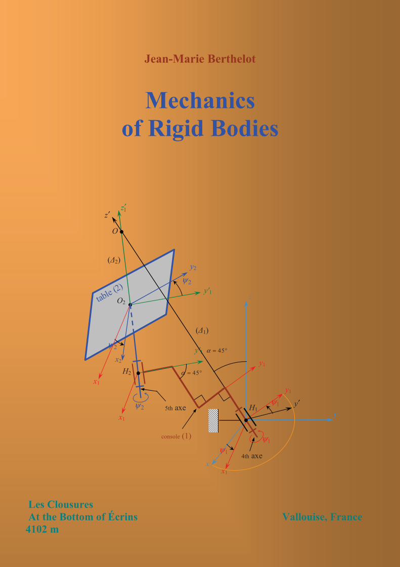
Jean-Marie Berthelot Mechanics of Rigid Bodies Les Clousures At the Bottom of Écrins Vallouise, France 4102 m z y' 1 y' 1 x 1 2 ψ 2 ψ x 2 O z ′ 1 z′ ( 2 ) y 2 y H 1 x 1 y′ x 1 ψ 1 ψ 1 ψ 4th axe y 1 y 1 5th axe console (1) ( 1 ) table (2) O 2 x 1 H 2 2 ψ 45 α = ° 45 α = °
Transcript of J.-M. Berthelot Mechanics of Rigid BodiesBerthelot+Mechanics+of+Rigid+Bodies.p… · reference...
Jean-Marie Berthelot
Mechanics of Rigid Bodies
Les Clousures At the Bottom of Écrins Vallouise, France 4102 m
z
y'1
y'1
x1
2ψ
2ψ
x2
O
z′1z′
(2) y2
yH1
x1
y′
x
1ψ
1ψ
1ψ
4th axe
y1
y1
5th axe
console (1)
(1)
table
(2)
O2
x1
H2
2ψ
45α = °
45α = °

Jean-Marie Berthelot
Mechanics of Rigid Bodies
Jean-Marie Berthelot is an Honorary Professor of Maine Univerty. He took part to
the installation of the Institute for Advanced Materials and Mechanics (ISMANS),
Le Mans, France. His current research is on the mechanical behaviour of
composite materials and structures. He has published extensively in the area of
composite materials and is the author of numerous international papers and
textbooks, in particular a textbook entitled Composite Materials, Mechanical
Behavior and Structural Analysis published by Springer, New York, in 1999.
see www.compomechaclimb.com..

Jean-Marie Berthelot
Mechanichs of Rigid Bodies
Les Clousures At the Bottom of Écrins Vallouise, France 4102 m


Preface
The objective of this book is to develop the fundamental statements of the
Mechanics of Rigid Bodies. The text is designed for undergraduate courses of
Mechanical Engineering. The basic mathematical concepts are covered in the first
part, thereby making the book self-contained. The different parts of the book are
carefully developed to provide continuity of the concepts and theories. Finally the
text has been established so as to construct chapter after chapter a unified proce-
dure for analysing any mechanical system constituted of rigid bodies.
The first part, Mathematical Basics, introduces the usual concepts needed in
the study of mechanical systems: vector space R3, geometric space, vector deriva-
tives, curves. A chapter is devoted to torsors whose concept is the key of the book.
The general notion of “measure centre” is introduced in this chapter.
The second part, Kinematics, begins with the analysis of the motion of a point
(kinematics of point). Particular motions are next considered, with a chapter
related to motions with central acceleration. Next, the kinematics of a rigid body
is studied: parameter of situation, kinematic torsor, analysis of particular motions.
The change of reference system, which introduces the notion of “entrainment” has
been excluded deliberately from this part. The notion of “entrainment” is not
really assimilated by the studients at this level of the text. In fact this notion is
implicitly introduced by using the concept of kinematic torsor. The change of
reference system will be considered as a whole within the frame of Kinetics (Part
4). The last chapter analyses the kinematics of rigid bodies in contact.
The third part, Mechanical Actions, introduces first the general concepts of the
mechanical actions exerted on a rigid body or on a system of rigid bodies.
Represented by torsors, the mechanical actions have general properties which are
derived from the concepts considered previously for torsors. Thus, mechanical
actions are classified as forces, couples and arbitrary actions. Gravitation and
gravity are analysed. A chapter is devoted to the mechanical actions involved by
the connections between rigid bodies, whose concept is the basis of the techno-
logical design of mechanical systems. The introduction of the power developed by
a mechanical action simplifies greatly the restrictions imposed in the case of
perfect connections (connections without friction). In the last chapter, the investi-
gation of some problem of Statics will grow the reader familiar with the analysis
of mechanical actions exerted on a body or a system of bodies.
The fourth part, Kinetics of Rigid Bodies, introduces the tools needed to
analyse the problems of Dynamics: operator of inertia, kinetic torsor, dynamic
torsor and kinetic energy. Next, the problem of the change of reference system is
considered.
At this step, the reader has acquired the whole elements needed to analyse the
problems of Dynamics of a rigid body or a system of rigid bodies. This analysis is
developed in the fifth part Dynamics of Rigid Bodies. First, the general process
for analysing a problem of Dynamics is established. Next, particular problems are
considered. The process of analysis is always the same: kinematic analysis, kinetic
analysis, investigation of the mechanical actions, deriving the equations of Dyna-
mics as a consequence of the fundamental principle of dynamics, assumptions
vi Preface
on the physical nature of connections between bodies, solving the equations of
motion and the equations of connections. The designer will have to take an
interest in the parameters of the motion as well as in the mechanical actions
exerted at the level of connections to design the mechanical systems. The appli-
cation of the fundamental principle of dynamics allows us to derive the whole
equations of dynamics (equations of motion and equations of mechanical actions
at the level of connections). However, designer which takes an interest only in the
equations of motion needs a systematic tool for deriving these equations: the
Lagrange’s equations which are considered in the last chapter of part V.
In general, the equations of motions of a body or of a system of rigid bodies are
complex, and most of these equations can not be solved using an analytical
process. Now, mechanical engineers dispose of numerical tools (numerical pro-
cesses and microcomputers) needed to solve the motion equations, whatever the
complexity of these equations may be. The sixth part, Numerical procedures for
the Resolution of Motion Equations, is an introduction to the numerical processes
used to solve equations of motion. Examples are considered.
The correction of the exercises is reported at the end of the textbook. The
writing has been developed extensively and structured in such a way to improve
the capacity of the comprehension of the reader.
At the end of the textbook, the designer will have all the elements which allow
him to implement a complete and structured analysis of mechanical systems.
June 2015, Vallouise, Jean-Marie BERTHELOT
Note. The development of this textbook is based on a generalized use of the
concept of “torseur” (in French). We think that this concept is not really used in
the English textbooks. We will call this concept as “torsor”. In the textbook, the
English formulation was thus transposed from the French formulation.
The author would be highly grateful with whoever would bring any element likely
to be able to make progress the development, and thus the comprehension, of the
textbook.


Contents
Preface v
PART I Mathematical Basic Elements 1
Chapter 1 Vector Space 3 3
1.1 Definition of the Vector Space 3 . . . . . . . . . . . . . . . . . . . . . . . . . . . . . . . . 3
1.1.1 Vectors . . . . . . . . . . . . . . . . . . . . . . . . . . . . . . . . . . . . . . . . . . . . . . . . . . 3
1.1.2 Vector Addition . . . . . . . . . . . . . . . . . . . . . . . . . . . . . . . . . . . . . . . . . . . 3
1.1.3 Multiplication by a Scalar . . . . . . . . . . . . . . . . . . . . . . . . . . . . . . . . . . . . 4
1.2 Linear Dependence and Independence. Basis of 3 . . . . . . . . . . . . . . . . . 5
1.2.1 Linear Combination. . . . . . . . . . . . . . . . . . . . . . . . . . . . . . . . . . . . . . . . . 5
1.2.2 Linear Dependence and Independence . . . . . . . . . . . . . . . . . . . . . . . . . . . 5
1.2.3 Basis of the Vector Space 3 . . . . . . . . . . . . . . . . . . . . . . . . . . . . . . . . . 7
1.2.4 Components of a Vector . . . . . . . . . . . . . . . . . . . . . . . . . . . . . . . . . . . . . 7
1.3 Scalar Product . . . . . . . . . . . . . . . . . . . . . . . . . . . . . . . . . . . . . . . . . . . . . . . 8
1.3.1 Definition . . . . . . . . . . . . . . . . . . . . . . . . . . . . . . . . . . . . . . . . . . . . . . . . 8
1.3.2 Magnitude or Norm of a Vector . . . . . . . . . . . . . . . . . . . . . . . . . . . . . . . . 8
1.3.3 Analytical Expression of the Scalar Product in an Arbitrary Basis . . . . . . 9
1.3.4 Orthogonal Vectors . . . . . . . . . . . . . . . . . . . . . . . . . . . . . . . . . . . . . . . . . 9
1.3.5 Orthonormal Basis . . . . . . . . . . . . . . . . . . . . . . . . . . . . . . . . . . . . . . . . . . 9
1.3.6 Expression of the Scalar Product in an Orthonormal Basis . . . . . . . . . . . . 10
1.4 Vector Product . . . . . . . . . . . . . . . . . . . . . . . . . . . . . . . . . . . . . . . . . . . . . . . 10
1.4.1 Definition . . . . . . . . . . . . . . . . . . . . . . . . . . . . . . . . . . . . . . . . . . . . . . . . 10
1.4.2 Analytical Expression of the Vector Product in an Arbitrary Basis . . . . . . 11
1.4.3 Direct Basis . . . . . . . . . . . . . . . . . . . . . . . . . . . . . . . . . . . . . . . . . . . . . . . 11
1.4.4 Expression of the Vector Product in a Direct Basis. . . . . . . . . . . . . . . . . . 12
1.4.5 Mixed Product . . . . . . . . . . . . . . . . . . . . . . . . . . . . . . . . . . . . . . . . . . . . . 12
1.4.6 Property of the Double Vector Product . . . . . . . . . . . . . . . . . . . . . . . . . . 12
1.5 Bases of the Vector Space 3 . . . . . . . . . . . . . . . . . . . . . . . . . . . . . . . . . . . 13
1.5.1 Canonical Basis . . . . . . . . . . . . . . . . . . . . . . . . . . . . . . . . . . . . . . . . . . . . 13
1.5.2 Basis Change . . . . . . . . . . . . . . . . . . . . . . . . . . . . . . . . . . . . . . . . . . . . . . 13
Exercises . . . . . . . . . . . . . . . . . . . . . . . . . . . . . . . . . . . . . . . . . . . . . . . . . . . 16
Comments . . . . . . . . . . . . . . . . . . . . . . . . . . . . . . . . . . . . . . . . . . . . . . . . . . 17
Chapter 2 The Geometric Space 18
2.1 The Geometric Space Considered as Affine to the Vector Space 3 . . . . . 18
Contents ix
2.1.1 The Geometric Space . . . . . . . . . . . . . . . . . . . . . . . . . . . . . . . . . . . . . . . . 18
2.1.2 Consequences . . . . . . . . . . . . . . . . . . . . . . . . . . . . . . . . . . . . . . . . . . . . . 19
2.1.3 Distance between Two Points . . . . . . . . . . . . . . . . . . . . . . . . . . . . . . . . . 20
2.1.4 Angle between Two Bipoints . . . . . . . . . . . . . . . . . . . . . . . . . . . . . . . . . . 20
2.1.5 Reference Systems . . . . . . . . . . . . . . . . . . . . . . . . . . . . . . . . . . . . . . . . . . 21
2.2 Subspaces of the Geometric Space: Line, Plane . . . . . . . . . . . . . . . . . . . . . 222.2.1 Line . . . . . . . . . . . . . . . . . . . . . . . . . . . . . . . . . . . . . . . . . . . . . . . . . . . . . 22
2.2.2 Plane . . . . . . . . . . . . . . . . . . . . . . . . . . . . . . . . . . . . . . . . . . . . . . . . . . . 23
2.2.3 Lines and Planes with Same Directions . . . . . . . . . . . . . . . . . . . . . . . . . . 24
2.2.4 Orthogonal Lines and Planes . . . . . . . . . . . . . . . . . . . . . . . . . . . . . . . . . . 25
2.3 Characterization of the Position a Point of the Geometric Space . . . . . . . 262.3.1 Coordinate Axes . . . . . . . . . . . . . . . . . . . . . . . . . . . . . . . . . . . . . . . . . . . 26
2.3.2 Direct Orthonormal Reference System . . . . . . . . . . . . . . . . . . . . . . . . . . . 27
2.3.3 Cartesian Coordinates . . . . . . . . . . . . . . . . . . . . . . . . . . . . . . . . . . . . . . . 27
2.4 Plane and Line Equations . . . . . . . . . . . . . . . . . . . . . . . . . . . . . . . . . . . . . . 292.4.1 Cartesian Equation of a Plane . . . . . . . . . . . . . . . . . . . . . . . . . . . . . . . . . 29
2.4.2 Cartesian Equation of a Line . . . . . . . . . . . . . . . . . . . . . . . . . . . . . . . . . . 30
2.5 Change of Reference System . . . . . . . . . . . . . . . . . . . . . . . . . . . . . . . . . . . . 312.5.1 General Case . . . . . . . . . . . . . . . . . . . . . . . . . . . . . . . . . . . . . . . . . . . . . . 31
2.5.2 Refernce Systems with a Same Axis . . . . . . . . . . . . . . . . . . . . . . . . . . . . 32
2.5.3 Arbitrary Reference Systems with the Same Origin . . . . . . . . . . . . . . . . . 34
Exercises . . . . . . . . . . . . . . . . . . . . . . . . . . . . . . . . . . . . . . . . . . . . . . . . . . 37 Comments . . . . . . . . . . . . . . . . . . . . . . . . . . . . . . . . . . . . . . . . . . . . . . . . . 39
Chapter 3 Vector Function. Derivatives of a Vector Function 40
3.1 Vector Function of One Variable . . . . . . . . . . . . . . . . . . . . . . . . . . . . . . . . . 40 3.1.1 Definition . . . . . . . . . . . . . . . . . . . . . . . . . . . . . . . . . . . . . . . . . . . . . . . . 40
3.1.2 Derivative . . . . . . . . . . . . . . . . . . . . . . . . . . . . . . . . . . . . . . . . . . . . . . . . 40
3.1.3 Properties of the Vector Derivative . . . . . . . . . . . . . . . . . . . . . . . . . . . . . 41
3.1.4 Examples . . . . . . . . . . . . . . . . . . . . . . . . . . . . . . . . . . . . . . . . . . . . . . . . . 42
3.2 Vector Function of Two Variables . . . . . . . . . . . . . . . . . . . . . . . . . . . . . . . 443.2.1 Definition . . . . . . . . . . . . . . . . . . . . . . . . . . . . . . . . . . . . . . . . . . . . . . . . 44
3.2.2 Partial Derivatives . . . . . . . . . . . . . . . . . . . . . . . . . . . . . . . . . . . . . . . . . . 44
3.2.3 Examples . . . . . . . . . . . . . . . . . . . . . . . . . . . . . . . . . . . . . . . . . . . . . . . . 45
3.3 Vector Function of n Variables . . . . . . . . . . . . . . . . . . . . . . . . . . . . . . . . . . 453.3.1 Definitions . . . . . . . . . . . . . . . . . . . . . . . . . . . . . . . . . . . . . . . . . . . . . . . . 45
3.3.2 Examples . . . . . . . . . . . . . . . . . . . . . . . . . . . . . . . . . . . . . . . . . . . . . . . . . 46
Comments . . . . . . . . . . . . . . . . . . . . . . . . . . . . . . . . . . . . . . . . . . . . . . . . . . 49
Chapter 4 Elementary Concepts on Curves 50
4.1 Introduction . . . . . . . . . . . . . . . . . . . . . . . . . . . . . . . . . . . . . . . . . . . . . . . . . 50 4.2 Curvilinear Abscissa. Arc Length of a Curve . . . . . . . . . . . . . . . . . . . . . . . 51 4.3 Tangent. Normal. Radius of Curvature . . . . . . . . . . . . . . . . . . . . . . . . . . . . 52 4.4 Frenet Trihedron . . . . . . . . . . . . . . . . . . . . . . . . . . . . . . . . . . . . . . . . . . . . . 52 Exercise . . . . . . . . . . . . . . . . . . . . . . . . . . . . . . . . . . . . . . . . . . . . . . . . . . . . 54
Comments 54

x Contents
Chapter 5 Torsors 55
5.1 Definition and Properties of the Torsors . . . . . . . . . . . . . . . . . . . . . . . . . . 555.1.1 Definitions and notations . . . . . . . . . . . . . . . . . . . . . . . . . . . . . . . . . . . . . 55
5.1.2 Properties of the Moments . . . . . . . . . . . . . . . . . . . . . . . . . . . . . . . . . . . . 56
5.1.3 Vector Space of Torsors . . . . . . . . . . . . . . . . . . . . . . . . . . . . . . . . . . . . . 56
5.1.4 Scalar Invariant of a Torsor . . . . . . . . . . . . . . . . . . . . . . . . . . . . . . . . . . . 57
5.1.5 Product of Two Torsors . . . . . . . . . . . . . . . . . . . . . . . . . . . . . . . . . . . . . . 58
5.1.6 Moment of a Torsor about an Axis . . . . . . . . . . . . . . . . . . . . . . . . . . . . . . 58
5.1.7 Central Axis of a Torsor . . . . . . . . . . . . . . . . . . . . . . . . . . . . . . . . . . . . . 59
5.2 Particular Torsors. Resolution of an Arbitrary Torsor . . . . . . . . . . . . . . . 605.2.1 Slider . . . . . . . . . . . . . . . . . . . . . . . . . . . . . . . . . . . . . . . . . . . . . . . . . . . . 60
5.2.2 Couple-Torsor . . . . . . . . . . . . . . . . . . . . . . . . . . . . . . . . . . . . . . . . . . . . . 62
5.2.3 Arbitrary Torsor . . . . . . . . . . . . . . . . . . . . . . . . . . . . . . . . . . . . . . . . . . . 63
5.2.4 Conclusions . . . . . . . . . . . . . . . . . . . . . . . . . . . . . . . . . . . . . . . . . . . . . . 64
5.3 Torsors associated to a Field of Sliders Defined on a Domain of the Geometric Space . . . . . . . . . . . . . . . . . . . . . . . . . . . . . . . . . . . . . . . . 645.3.1 Torsor Associated to a Finite Set of Points . . . . . . . . . . . . . . . . . . . . . . . . 64
5.3.2 Torsor Associated to a Infinite Set of Points . . . . . . . . . . . . . . . . . . . . . . 65
5.3.3 Important Particular Case. Measure Centre . . . . . . . . . . . . . . . . . . . . . . . 67
Exercises . . . . . . . . . . . . . . . . . . . . . . . . . . . . . . . . . . . . . . . . . . . . . . . . . . . . 70 Comments . . . . . . . . . . . . . . . . . . . . . . . . . . . . . . . . . . . . . . . . . . . . . . . . . . . 72
PART II Kinematics 73
Chapter 6 Kinematics of Point 75
6.1 Introduction . . . . . . . . . . . . . . . . . . . . . . . . . . . . . . . . . . . . . . . . . . . . . . . . . 75 6.2 Trajectory and Kinematic Vectors of a Point . . . . . . . . . . . . . . . . . . . . . . . 756.2.1 Trajectory . . . . . . . . . . . . . . . . . . . . . . . . . . . . . . . . . . . . . . . . . . . . . . . . 76
6.2.2 Kinematic Vectors . . . . . . . . . . . . . . . . . . . . . . . . . . . . . . . . . . . . . . . . . . 77
6.2.3 Tangential and Normal Components of Kinematic Vectors . . . . . . . . . . . 78
6.2.4 Different Types of Motions . . . . . . . . . . . . . . . . . . . . . . . . . . . . . . . . . . . 79
6.3 Expressions of the Components of Kinematic Vectors as Functions of Cartesian and Cylindrical Coordinates . . . . . . . . . . . . . . . . . . . . . . . . . . . 81
6.3.1 Cartesian Coordinates . . . . . . . . . . . . . . . . . . . . . . . . . . . . . . . . . . . . . . . 81
6.3.2 Cylindrical Coordinates . . . . . . . . . . . . . . . . . . . . . . . . . . . . . . . . . . . . . . 82
Exercises . . . . . . . . . . . . . . . . . . . . . . . . . . . . . . . . . . . . . . . . . . . . . . . . . . . . 83 Comments . . . . . . . . . . . . . . . . . . . . . . . . . . . . . . . . . . . . . . . . . . . . . . . . . . . 83
Chapter 7 Study of Particular Motions 84
7.1 Motions with Rectilinear Trajectory . . . . . . . . . . . . . . . . . . . . . . . . . . . . . . 84 7.1.1 General Considerations . . . . . . . . . . . . . . . . . . . . . . . . . . . . . . . . . . . . . . 84
7.1.2 Uniform Rectilinear Motion . . . . . . . . . . . . . . . . . . . . . . . . . . . . . . . . . . 85
7.1.3 Uniformly Varied Rectilinear Motion . . . . . . . . . . . . . . . . . . . . . . . . . . . 85
7.1.4 Simple Harmonic Rectilinear Motion . . . . . . . . . . . . . . . . . . . . . . . . . . . . 86
7.2 Motions with a Circular Trajectory . . . . . . . . . . . . . . . . . . . . . . . . . . . . . . 87 7.2.1 General Equations . . . . . . . . . . . . . . . . . . . . . . . . . . . . . . . . . . . . . . . . . . 87

Contents xi
7.2.2 Uniform Circular Motion . . . . . . . . . . . . . . . . . . . . . . . . . . . . . . . . . . . . 88
7.2.3 Uniformly Varied Circular Motion . . . . . . . . . . . . . . . . . . . . . . . . . . . . . . 89
7.3 Motions with a Contant Acceleration Vector . . . . . . . . . . . . . . . . . . . . . . . 90 7.3.1 General Equations . . . . . . . . . . . . . . . . . . . . . . . . . . . . . . . . . . . . . . . . . . 90
7.3.2 Study of the case where the Trajectory is Rectilinear . . . . . . . . . . . . . . . . 91
7.3.3 Study of the case where the Trajectory is Parabolic . . . . . . . . . . . . . . . . . 92
7.4 Helicoidal Motion . . . . . . . . . . . . . . . . . . . . . . . . . . . . . . . . . . . . . . . . . . . . 947.5 Cycloidal Motion . . . . . . . . . . . . . . . . . . . . . . . . . . . . . . . . . . . . . . . . . . . . . 96 Exercises . . . . . . . . . . . . . . . . . . . . . . . . . . . . . . . . . . . . . . . . . . . . . . . . . . . . 98 Comments . . . . . . . . . . . . . . . . . . . . . . . . . . . . . . . . . . . . . . . . . . . . . . . . . . . 99
Chapter 8 Motions with Central Acceleration 100
8.1 General Properties . . . . . . . . . . . . . . . . . . . . . . . . . . . . . . . . . . . . . . . . . . . . 1008.1.1 Definition . . . . . . . . . . . . . . . . . . . . . . . . . . . . . . . . . . . . . . . . . . . . . . . . 100
8.1.2 A Motion with a Central Acceleration is a Plane Trajectory
Motion . . . . . . . . . . . . . . . . . . . . . . . . . . . . . . . . . . . . . . . . . . . . . . . . . . 100
8.1.3 Areal Velocity . . . . . . . . . . . . . . . . . . . . . . . . . . . . . . . . . . . . . . . . . . . . . 101
8.1.4 Area Law . . . . . . . . . . . . . . . . . . . . . . . . . . . . . . . . . . . . . . . . . . . . . . . . . 102
8.1.5 Expression of the Kinematic Vectors . . . . . . . . . . . . . . . . . . . . . . . . . . . . 102
8.1.6 Polar Equation of the Trajectory . . . . . . . . . . . . . . . . . . . . . . . . . . . . . . . 102
8.1.7 Motions for which ( ) 2( , )Ta M t OMω= −
. . . . . . . . . . . . . . . . . . . . . . . . . . 103
8.2 Motions with Central Acceleration for which ( )
3( , )T OM
a M t KOM
= −
. . . . 104
8.2.1 Equations of the Trajectories . . . . . . . . . . . . . . . . . . . . . . . . . . . . . . . . . . 104
8.2.2 Study of the Trajectories . . . . . . . . . . . . . . . . . . . . . . . . . . . . . . . . . . . . . 105
8.2.3 Velocity Magnitude at a Point of the Trajectory . . . . . . . . . . . . . . . . . . . . 107
8.2.4 Elliptic Motion. Kepler’s Laws . . . . . . . . . . . . . . . . . . . . . . . . . . . . . . . . 108
Comments . . . . . . . . . . . . . . . . . . . . . . . . . . . . . . . . . . . . . . . . . . . . . . . . . . . 110
Chapter 9 Kinematics of Rigid Body 111
9.1 General Considerations . . . . . . . . . . . . . . . . . . . . . . . . . . . . . . . . . . . . . . . . 1119.1.1 Notion of Rigid Body . . . . . . . . . . . . . . . . . . . . . . . . . . . . . . . . . . . . . . . 111
9.1.2 Locating a Rigid Body . . . . . . . . . . . . . . . . . . . . . . . . . . . . . . . . . . . . . . . 111
9.2 Relations between the Trajectories and the Kinematic Vectors of Two Points Attached to a Solid . . . . . . . . . . . . . . . . . . . . . . . . . . . . . . . . 113
9.2.1 Relation between the Trajectories . . . . . . . . . . . . . . . . . . . . . . . . . . . . . . 113
9.2.2 Relation between the Velocity Vectors. . . . . . . . . . . . . . . . . . . . . . . . . . . 114
9.2.3 Expression of the Instantaneous Vector of Rotation . . . . . . . . . . . . . . . . . 115
9.2.4 Kinematic Torsor . . . . . . . . . . . . . . . . . . . . . . . . . . . . . . . . . . . . . . . . . . . 116
9.2.5 Relation between the Acceleration Vectors . . . . . . . . . . . . . . . . . . . . . . . 117
9.3 Generalization of the Composition of Motions . . . . . . . . . . . . . . . . . . . . . . 1189.3.1 Composition of Kinematic Torsors . . . . . . . . . . . . . . . . . . . . . . . . . . . . . 118
9.3.2 Inverse Motions . . . . . . . . . . . . . . . . . . . . . . . . . . . . . . . . . . . . . . . . . . . . 120
9.4 Examples of Solid Motions . . . . . . . . . . . . . . . . . . . . . . . . . . . . . . . . . . . . . . 1219.4.1 Motion of Rotation about a Fixed Axis . . . . . . . . . . . . . . . . . . . . . . . . . . 121
9.4.2 Translation Motion of a Rigid Body . . . . . . . . . . . . . . . . . . . . . . . . . . . . . 124
xii Contents
9.4.3 Motion of a Body Subjected to a Cylindrical Joint . . . . . . . . . . . . . . . . . . 125
9.4.4 Motion of Rotation about a Fixed Point . . . . . . . . . . . . . . . . . . . . . . . . . . 127
9.4.5 Plane Motion . . . . . . . . . . . . . . . . . . . . . . . . . . . . . . . . . . . . . . . . . . . . . . 129
Exercises . . . . . . . . . . . . . . . . . . . . . . . . . . . . . . . . . . . . . . . . . . . . . . . . . . . . 134 Comments . . . . . . . . . . . . . . . . . . . . . . . . . . . . . . . . . . . . . . . . . . . . . . . . . . . 136
Chapter 10 Kinematics of Rigid Bodies in Contact 137
10.1 Kinematics of Two Solids in Contact . . . . . . . . . . . . . . . . . . . . . . . . . . . . . . 137 10.1.1 Solids in Contact at a Point. Sliding . . . . . . . . . . . . . . . . . . . . . . . . . . . . . 137
10.1.2 Spinning and Rolling . . . . . . . . . . . . . . . . . . . . . . . . . . . . . . . . . . . . . . . . 138
10.1.3 Conclusions . . . . . . . . . . . . . . . . . . . . . . . . . . . . . . . . . . . . . . . . . . . . . . . 139
10.1.4 Solids in Contact in Several points . . . . . . . . . . . . . . . . . . . . . . . . . . . . . . 140
10.2 Transmission of a Motion of Rotation . . . . . . . . . . . . . . . . . . . . . . . . . . . . . 14010.2.1 Général Elements . . . . . . . . . . . . . . . . . . . . . . . . . . . . . . . . . . . . . . . . . . 140
10.2.2 Transmission by Friction . . . . . . . . . . . . . . . . . . . . . . . . . . . . . . . . . . . . . 141
10.2.3 Gear Transmission . . . . . . . . . . . . . . . . . . . . . . . . . . . . . . . . . . . . . . . . . . 145
10.2.4 Belt Transmission . . . . . . . . . . . . . . . . . . . . . . . . . . . . . . . . . . . . . . . . . . 148
Exercises . . . . . . . . . . . . . . . . . . . . . . . . . . . . . . . . . . . . . . . . . . . . . . . . . . . . 150 Comments . . . . . . . . . . . . . . . . . . . . . . . . . . . . . . . . . . . . . . . . . . . . . . . . . . . 151
PART III The Mechanical Actions 153
Chapter 11 General Elements on the Mechanical Actions 155
11.1 Concepts Relative to the Mechanical Actions . . . . . . . . . . . . . . . . . . . . . . . 15511.1.1 Notion of Mechanical Action . . . . . . . . . . . . . . . . . . . . . . . . . . . . . . . . . . 155
11.1.2 Representation of a Mechanical Action . . . . . . . . . . . . . . . . . . . . . . . . . . 155
11.1.3 Classification of the Mechanical Actions . . . . . . . . . . . . . . . . . . . . . . . . . 156
11.1.4 Mechanical Actions Exerting between Material Sets . . . . . . . . . . . . . . . . 158
11.1.5 External Mechanical Actions Exerting on a Material Set . . . . . . . . . . . . . 158
11.2 Different Types of Mechanical Actions . . . . . . . . . . . . . . . . . . . . . . . . . . . . 15911.2.1 Physical Natures of the Mechanical Actions . . . . . . . . . . . . . . . . . . . . . . . 159
11.2.2 Environnement and Effective Actions . . . . . . . . . . . . . . . . . . . . . . . . . . . 159
11.3 Power and Work . . . . . . . . . . . . . . . . . . . . . . . . . . . . . . . . . . . . . . . . . . . . . 16011.3.1 Definition of the Power . . . . . . . . . . . . . . . . . . . . . . . . . . . . . . . . . . . . . . 160
11.3.2 Change of Reference System . . . . . . . . . . . . . . . . . . . . . . . . . . . . . . . . . . 161
11.3.3 Potential Energy . . . . . . . . . . . . . . . . . . . . . . . . . . . . . . . . . . . . . . . . . . . 161
11.3.4 Work . . . . . . . . . . . . . . . . . . . . . . . . . . . . . . . . . . . . . . . . . . . . . . . . . . . . 162
11.3.5 Power and Work of a Force . . . . . . . . . . . . . . . . . . . . . . . . . . . . . . . . . . . 163
11.3.6 Set of Rigid Bodies . . . . . . . . . . . . . . . . . . . . . . . . . . . . . . . . . . . . . . . . . 164
Exercises . . . . . . . . . . . . . . . . . . . . . . . . . . . . . . . . . . . . . . . . . . . . . . . . . . . 165 Comments . . . . . . . . . . . . . . . . . . . . . . . . . . . . . . . . . . . . . . . . . . . . . . . . . . . 167
Chapter 12 Gravitation. Gravity. Mass Centre 169
12.1 Phenomenon of Gravitation . . . . . . . . . . . . . . . . . . . . . . . . . . . . . . . . . . . . 16912.1.1 Law of Gravitation 169

Contents xiii
12.1.2 Gravitational Field . . . . . . . . . . . . . . . . . . . . . . . . . . . . . . . . . . . . . . . . . . 170
12.1.3 Action of gravitation induced by a Solid Sphere . . . . . . . . . . . . . . . . . . . 170
12.1.4 Action of gravitation induced by the Earth . . . . . . . . . . . . . . . . . . . . . . . . 172
12.2 Action of Gravity . . . . . . . . . . . . . . . . . . . . . . . . . . . . . . . . . . . . . . . . . . . . . 17312.2.1 Gravity Field Induced by the Earth . . . . . . . . . . . . . . . . . . . . . . . . . . . . . 173
12.2.2 Action of Gravity Exerted on a Material System . . . . . . . . . . . . . . . . . . . 174
12.2.3 Power Developed by the Action of Gravity . . . . . . . . . . . . . . . . . . . . . . . 175
12.3 Determination of Mass Centres . . . . . . . . . . . . . . . . . . . . . . . . . . . . . . . . . . 17712.3.1 Mass Centre of a Material System . . . . . . . . . . . . . . . . . . . . . . . . . . . . . . 177
12.3.2 Mass Centre of the Union of Two Sets . . . . . . . . . . . . . . . . . . . . . . . . . . 178
12.3.3 Mass Centre of a Homogeneous Set . . . . . . . . . . . . . . . . . . . . . . . . . . . . 179
12.3.4 Homogeneous Bodies with Geometrical Symmetries . . . . . . . . . . . . . . . . 180
12.4 Examples of Determination of Mass Centres . . . . . . . . . . . . . . . . . . . . . . . 18112.4.1 Homogeneous Solid Hemisphere . . . . . . . . . . . . . . . . . . . . . . . . . . . . . . . 181
12.4.2 Homogeneous Solid with Complex Geometry . . . . . . . . . . . . . . . . . . . . . 182
12.4.3 Non-Homogeneous Solid . . . . . . . . . . . . . . . . . . . . . . . . . . . . . . . . . . . . 183
Exercises . . . . . . . . . . . . . . . . . . . . . . . . . . . . . . . . . . . . . . . . . . . . . . . . . . . 184 Comments . . . . . . . . . . . . . . . . . . . . . . . . . . . . . . . . . . . . . . . . . . . . . . . . . . 185
Chapter 13 Actions of Contact between Solids. Connections 186
13.1 Laws of Contact between Solids . . . . . . . . . . . . . . . . . . . . . . . . . . . . . . . . . . 186 13.1.1 Introduction . . . . . . . . . . . . . . . . . . . . . . . . . . . . . . . . . . . . . . . . . . . . . . . 186
13.1.2 Contact in a Point . . . . . . . . . . . . . . . . . . . . . . . . . . . . . . . . . . . . . . . . . . 186
13.1.3 Couples of Rolling and Spinning . . . . . . . . . . . . . . . . . . . . . . . . . . . . . . . 191
13.2 Connections . . . . . . . . . . . . . . . . . . . . . . . . . . . . . . . . . . . . . . . . . . . . . . . . . 19213.2.1 Introduction . . . . . . . . . . . . . . . . . . . . . . . . . . . . . . . . . . . . . . . . . . . . . . . 192
13.2.2 Classification of Connections. . . . . . . . . . . . . . . . . . . . . . . . . . . . . . . . . . 193
13.2.3 Actions of Connection . . . . . . . . . . . . . . . . . . . . . . . . . . . . . . . . . . . . . . . 197
13.2.4 Connection without Friction . . . . . . . . . . . . . . . . . . . . . . . . . . . . . . . . . . 198
13.2.5 Connection with Friction . . . . . . . . . . . . . . . . . . . . . . . . . . . . . . . . . . . . 202
Comments . . . . . . . . . . . . . . . . . . . . . . . . . . . . . . . . . . . . . . . . . . . . . . . . . . . 203
Chapter 14 Statics of Rigid Bodies 204
14.1 Introduction . . . . . . . . . . . . . . . . . . . . . . . . . . . . . . . . . . . . . . . . . . . . . . . . . 204 14.2 Law of Statics . . . . . . . . . . . . . . . . . . . . . . . . . . . . . . . . . . . . . . . . . . . . . . . . 20414.2.1 Case of a Rigid Body . . . . . . . . . . . . . . . . . . . . . . . . . . . . . . . . . . . . . . . . 204
14.2.2 Case of a Set of Rigid Bodies . . . . . . . . . . . . . . . . . . . . . . . . . . . . . . . . . . 205
14.2.3 Mutual Actions . . . . . . . . . . . . . . . . . . . . . . . . . . . . . . . . . . . . . . . . . . . . 206
14.3 Statics of Wires or Flexible Cables . . . . . . . . . . . . . . . . . . . . . . . . . . . . . . . 20714.3.1 Mechanical Action Exerted by a Wire or a Flexible Cable . . . . . . . . . . . . 207
14.3.2 Equation of Statics of a Wire . . . . . . . . . . . . . . . . . . . . . . . . . . . . . . . . . . 208
14.3.3 Wire or Flexible Cable Submitted to the Gravity . . . . . . . . . . . . . . . . . . . 209
14.3.4 Contact of a Wire with a Rigid Body . . . . . . . . . . . . . . . . . . . . . . . . . . . . 210
14.4 Examples of Equilibrium . . . . . . . . . . . . . . . . . . . . . . . . . . . . . . . . . . . . . . 21214.4.1 Case of a Rigid Body . . . . . . . . . . . . . . . . . . . . . . . . . . . . . . . . . . . . . . . . 212
14.4.2 Case of a System of Two Rigid Bodies . . . . . . . . . . . . . . . . . . . . . . . . . . 217
Exercises . . . . . . . . . . . . . . . . . . . . . . . . . . . . . . . . . . . . . . . . . . . . . . . . . . . 222 Comments 223
Contents xiv
PART IV Kinetics of Rigid Bodies 225
Chapter 15 The Operator of Inertia 227
15.1 Introduction to the Operator of Inertia . . . . . . . . . . . . . . . . . . . . . . . . . . . 22715.1.1 Operator Associated to a Vector Product . . . . . . . . . . . . . . . . . . . . . . . . . 227
15.1.2 Extending the Preceding Concept . . . . . . . . . . . . . . . . . . . . . . . . . . . . . . 228
15.1.3 The Operator of Inertia . . . . . . . . . . . . . . . . . . . . . . . . . . . . . . . . . . . . . . 229
15.2 Change of Coordinate System . . . . . . . . . . . . . . . . . . . . . . . . . . . . . . . . . . . 23015.2.1 Change of Origin . . . . . . . . . . . . . . . . . . . . . . . . . . . . . . . . . . . . . . . . . . 230
15.2.2 Relations of Huyghens . . . . . . . . . . . . . . . . . . . . . . . . . . . . . . . . . . . . . . 232
15.2.3 Diagonalisation of the Matrix of Inertia . . . . . . . . . . . . . . . . . . . . . . . . . 232
15.2.4 Change of Basis . . . . . . . . . . . . . . . . . . . . . . . . . . . . . . . . . . . . . . . . . . . 233
15.3 Moments of Inertia with respect to a point, an axis, a plane . . . . . . . . . . . 23415.3.1 Definitions . . . . . . . . . . . . . . . . . . . . . . . . . . . . . . . . . . . . . . . . . . . . . . . 234
15.3.2 Relations between the Moments of Inertia . . . . . . . . . . . . . . . . . . . . . . . . 235
15.3.3 Case of a Plane Solid . . . . . . . . . . . . . . . . . . . . . . . . . . . . . . . . . . . . . . . 235
15.3.4 Moment of Inertia with respect to an Arbitrary Axis . . . . . . . . . . . . . . . . 236
15.4 Determination of Matrices of Inertia . . . . . . . . . . . . . . . . . . . . . . . . . . . . . 23715.4.1 Solids with Material Symmetries . . . . . . . . . . . . . . . . . . . . . . . . . . . . . . 237
15.4.2 Solids having a Symmetry of Revolution . . . . . . . . . . . . . . . . . . . . . . . . 239
15.4.3 Solids with Spherical Symmetry . . . . . . . . . . . . . . . . . . . . . . . . . . . . . . . 241
15.4.4 Associativity . . . . . . . . . . . . . . . . . . . . . . . . . . . . . . . . . . . . . . . . . . . . . . 242
15.5 Matrices of Inertia of Homogeneous Bodies . . . . . . . . . . . . . . . . . . . . . . . . 24415.5.1 One-Dimensional Solids . . . . . . . . . . . . . . . . . . . . . . . . . . . . . . . . . . . . . 244
15.5.2 Two-Dimensional Solids . . . . . . . . . . . . . . . . . . . . . . . . . . . . . . . . . . . . 245
15.5.3 Three-Dimensional Solids . . . . . . . . . . . . . . . . . . . . . . . . . . . . . . . . . . . 249
Exercises . . . . . . . . . . . . . . . . . . . . . . . . . . . . . . . . . . . . . . . . . . . . . . . . . . . 253 Comments . . . . . . . . . . . . . . . . . . . . . . . . . . . . . . . . . . . . . . . . . . . . . . . . . . 254
Chapter 16 Kinetic and Dynamic Torsors. Kinetic Energy 255
16.1 Kinetic Torsor . . . . . . . . . . . . . . . . . . . . . . . . . . . . . . . . . . . . . . . . . . . . . . . 25516.1.1 Definition . . . . . . . . . . . . . . . . . . . . . . . . . . . . . . . . . . . . . . . . . . . . . . . . 255
16.1.2 Kinetic Torsor Associated to the Motion of a Body . . . . . . . . . . . . . . . . . 256
16.1.3 Kinetic Torsor for a Set of Bodies . . . . . . . . . . . . . . . . . . . . . . . . . . . . . . 257
16.2 Dynamic Torsor. . . . . . . . . . . . . . . . . . . . . . . . . . . . . . . . . . . . . . . . . . . . . . 25816.2.1 Definition . . . . . . . . . . . . . . . . . . . . . . . . . . . . . . . . . . . . . . . . . . . . . . . . 258
16.2.2 Dynamic Torsor Associated to the Motion of a Body . . . . . . . . . . . . . . . 258
16.2.3 Dynamic Torsor for a Set of Bodies . . . . . . . . . . . . . . . . . . . . . . . . . . . . 259
16.2.4 Relation with the Kinetic Energy . . . . . . . . . . . . . . . . . . . . . . . . . . . . . . 260
16.3 Kinetic Energy . . . . . . . . . . . . . . . . . . . . . . . . . . . . . . . . . . . . . . . . . . . . . . . 26016.3.1 Definition . . . . . . . . . . . . . . . . . . . . . . . . . . . . . . . . . . . . . . . . . . . . . . . . 260
16.3.2 Kinetic Energy of a Body . . . . . . . . . . . . . . . . . . . . . . . . . . . . . . . . . . . . 261
16.3.3 Kinetic Energy of a Set of Solids . . . . . . . . . . . . . . . . . . . . . . . . . . . . . . 262
16.3.4 Derivative of the Kinetic Energy of a Solid with respect to Time . . . . . . 262
Exercises . . . . . . . . . . . . . . . . . . . . . . . . . . . . . . . . . . . . . . . . . . . . . . . . . . . 263 Comments . . . . . . . . . . . . . . . . . . . . . . . . . . . . . . . . . . . . . . . . . . . . . . . . . . 264

Contents xv
Chapter 17 Change of Reference System 265
17.1 Kinematics of Change of Reference . . . . . . . . . . . . . . . . . . . . . . . . . . . . . . 26517.1.1 Relation between the Kinematic Torsors . . . . . . . . . . . . . . . . . . . . . . . . . 265
17.1.2 Relation between the Velocity Vectors. Velocity of Entrainment . . . . . . 266
17.1.3 Composition of Acceleration Vectors . . . . . . . . . . . . . . . . . . . . . . . . . . . 268
17.2 Dynamic Torsors . . . . . . . . . . . . . . . . . . . . . . . . . . . . . . . . . . . . . . . . . . . . . 26917.2.1 Inertia Torsor of Entrainment . . . . . . . . . . . . . . . . . . . . . . . . . . . . . . . . . 270
17.2.2 Inertia Torsor of Coriolis . . . . . . . . . . . . . . . . . . . . . . . . . . . . . . . . . . . . 271
17.2.3 Relation between the Dynamic Torsors Defined relatively
to Two Different References . . . . . . . . . . . . . . . . . . . . . . . . . . . . . . . . . . 272
Comments . . . . . . . . . . . . . . . . . . . . . . . . . . . . . . . . . . . . . . . . . . . . . . . . . . 273
PART V Dynamics of Rigid Bodies 275
Chapter 18 The Fundamental Principle of Dynamics and its Consequences 277
18.1 Fundamental Principle. . . . . . . . . . . . . . . . . . . . . . . . . . . . . . . . . . . . . . . . . 277 18.1.1 Statement of the Fundamental Principle of Dynamics . . . . . . . . . . . . . . . 277
18.1.2 Class of Galilean Reference Systems . . . . . . . . . . . . . . . . . . . . . . . . . . . 277
18.1.3 Vector Equations Deduced from the Fundamental Principle . . . . . . . . . . 278
18.1.4 Scalar Equations Deduced from the Fundamental Principle . . . . . . . . . . . 279
18.2 Mutual Actions . . . . . . . . . . . . . . . . . . . . . . . . . . . . . . . . . . . . . . . . . . . . . . 28018.2.1 Theorem of Mutual Actions . . . . . . . . . . . . . . . . . . . . . . . . . . . . . . . . . . 280
18.2.2 Transmission of Mechanical Actions . . . . . . . . . . . . . . . . . . . . . . . . . . . 281
18.3 Theorem of Power-Energy. . . . . . . . . . . . . . . . . . . . . . . . . . . . . . . . . . . . . . 281 18.3.1 Case of One Solid . . . . . . . . . . . . . . . . . . . . . . . . . . . . . . . . . . . . . . . . . 281
18.3.2 Case of a Set of Bodies . . . . . . . . . . . . . . . . . . . . . . . . . . . . . . . . . . . . . . 282
18.3.3 Mechanical Actions with Potential Energy . . . . . . . . . . . . . . . . . . . . . . . 283
18.4 Application of the Fundamental Principle to the Study of the Motion of a Free Body in a Galilean Reference . . . . . . . . . . . . . . . . . . . . . . . . . . . 284
18.4.1 General Problem . . . . . . . . . . . . . . . . . . . . . . . . . . . . . . . . . . . . . . . . . . . 284
18.4.2 Particular Cases . . . . . . . . . . . . . . . . . . . . . . . . . . . . . . . . . . . . . . . . . . . 286
18.5 Application to the Solar System. . . . . . . . . . . . . . . . . . . . . . . . . . . . . . . . . . 288 18.5.1 Galilean Reference . . . . . . . . . . . . . . . . . . . . . . . . . . . . . . . . . . . . . . . . 288
18.5.2 Motion of Planets . . . . . . . . . . . . . . . . . . . . . . . . . . . . . . . . . . . . . . . . . . 290
18.5.3 The Earth in the Solar System . . . . . . . . . . . . . . . . . . . . . . . . . . . . . . . . . 290
Comments . . . . . . . . . . . . . . . . . . . . . . . . . . . . . . . . . . . . . . . . . . . . . . . . . . 291
Chapter 19 The Fundamental Equation of Dynamics in Different References 293
19.1 General Elements . . . . . . . . . . . . . . . . . . . . . . . . . . . . . . . . . . . . . . . . . . . . 293 19.1.1 Fundamental Equation of Dynamics in a Non Galilean Reference . . . . . 293
19.1.2 The Reference Systems used in Mechanics . . . . . . . . . . . . . . . . . . . . . . . 294
19.2 Fundamental Relation of Dynamics in the Geocentric Reference . . . . . . . 29519.2.1 General Equations . . . . . . . . . . . . . . . . . . . . . . . . . . . . . . . . . . . . . . . . . 295

Contents xvi
19.2.2 Case of a Solid Located at the Vicinity of the Earth . . . . . . . . . . . . . . . . 297
19.3 Fundamental Relation in a Reference Attached to the Earth . . . . . . . . . . 29819.3.1 Equations of Motion . . . . . . . . . . . . . . . . . . . . . . . . . . . . . . . . . . . . . . . . 298
19.3.2 Action of Earthly Gravity . . . . . . . . . . . . . . . . . . . . . . . . . . . . . . . . . . . . 299
19.3.3 Conclusions on the Equations of Dynamics in a Reference
Attached to the Earth . . . . . . . . . . . . . . . . . . . . . . . . . . . . . . . . . . . . . . 300
19.4 Equations of Dynamics of a Body with respect to a Reference whose the Motion is Known Relatively to the Earth . . . . . . . . . . . . . . . . 301
Comments . . . . . . . . . . . . . . . . . . . . . . . . . . . . . . . . . . . . . . . . . . . . . . . . . . 303
Chapter 20 General Process for Analysing a Problem of Dynamics of Rigid Bodies 304
20.1 Dynamics of Rigid Body . . . . . . . . . . . . . . . . . . . . . . . . . . . . . . . . . . . . . . . 304 20.1.1 General Equations . . . . . . . . . . . . . . . . . . . . . . . . . . . . . . . . . . . . . . . . . 304
20.1.2 General Process of Analysis . . . . . . . . . . . . . . . . . . . . . . . . . . . . . . . . . . 305
20.2 Dynamics of a Set of Bodies . . . . . . . . . . . . . . . . . . . . . . . . . . . . . . . . . . . . 306 20.3 Conclusion . . . . . . . . . . . . . . . . . . . . . . . . . . . . . . . . . . . . . . . . . . . . . . . . . . 307 Comments . . . . . . . . . . . . . . . . . . . . . . . . . . . . . . . . . . . . . . . . . . . . . . . . . . 308
Chapter 21 Dynamics of Systems with One Degree of Freedom Analysis of Vibrations 309
21.1 General Equations . . . . . . . . . . . . . . . . . . . . . . . . . . . . . . . . . . . . . . . . . . . . 309 21.1.1 Introduction . . . . . . . . . . . . . . . . . . . . . . . . . . . . . . . . . . . . . . . . . . . . . . 309
21.1.2 Parameters of Situation . . . . . . . . . . . . . . . . . . . . . . . . . . . . . . . . . . . . . . 310
21.1.3 Kinematics . . . . . . . . . . . . . . . . . . . . . . . . . . . . . . . . . . . . . . . . . . . . . . 310
21.1.4 Kinetics . . . . . . . . . . . . . . . . . . . . . . . . . . . . . . . . . . . . . . . . . . . . . . . . . 310
21.1.5 Mechanical Actions Exerted on the Solid . . . . . . . . . . . . . . . . . . . . . . . . 311
21.1.6 Application of the Fundamental Principle . . . . . . . . . . . . . . . . . . . . . . . . 311
21.2 Vibrations without Friction . . . . . . . . . . . . . . . . . . . . . . . . . . . . . . . . . . . . 313 21.2.1 Equation of Motion . . . . . . . . . . . . . . . . . . . . . . . . . . . . . . . . . . . . . . . . . 313
21.2.2 Free Vibrations . . . . . . . . . . . . . . . . . . . . . . . . . . . . . . . . . . . . . . . . . . . . 313
21.2.3 Forced Vibrations. Steady State . . . . . . . . . . . . . . . . . . . . . . . . . . . . . . . 314
21.3 Vibrations with Viscous Damping . . . . . . . . . . . . . . . . . . . . . . . . . . . . . . 31821.3.1 Equation of Motion with Viscous Damping . . . . . . . . . . . . . . . . . . . . . . 318
21.3.2 Free Vibrations . . . . . . . . . . . . . . . . . . . . . . . . . . . . . . . . . . . . . . . . . . . . 318
21.3.3 Vibrations in the case of a Harmonic Disturbing Force . . . . . . . . . . . . . . 324
21.3.4 Forced Vibrations in the case of a Periodic Disturbing Force. . . . . . . . . . 331
21.3.5 Vibrations in the case of an Arbitrary Disturbing Force . . . . . . . . . . . . . . 332
21.3.6 Forced Vibrations in the case of a Motion Imposed to the Support . . . . . 333
21.4 Vibrations with Dry Friction . . . . . . . . . . . . . . . . . . . . . . . . . . . . . . . . . . . 33621.4.1 Equations of Motion . . . . . . . . . . . . . . . . . . . . . . . . . . . . . . . . . . . . . . . . 336
21.4.2 Free Vibrations . . . . . . . . . . . . . . . . . . . . . . . . . . . . . . . . . . . . . . . . . . . . 337
21.5 Equivalent Viscous Damping . . . . . . . . . . . . . . . . . . . . . . . . . . . . . . . . . . . 33921.5.1 Introduction . . . . . . . . . . . . . . . . . . . . . . . . . . . . . . . . . . . . . . . . . . . . . . 339
21.5.2 Energy Dissipated in the case of Viscous Damping . . . . . . . . . . . . . . . . 340
21.5.3 Stuctural Damping . . . . . . . . . . . . . . . . . . . . . . . . . . . . . . . . . . . . . . . . . 340
Contents xvii
21.5.4 Dry Friction . . . . . . . . . . . . . . . . . . . . . . . . . . . . . . . . . . . . . . . . . . . . . . 342
21.5.5 Fluid Friction . . . . . . . . . . . . . . . . . . . . . . . . . . . . . . . . . . . . . . . . . . . . . 343
21.5.6 Conclusion . . . . . . . . . . . . . . . . . . . . . . . . . . . . . . . . . . . . . . . . . . . . . . . 345
Exercises . . . . . . . . . . . . . . . . . . . . . . . . . . . . . . . . . . . . . . . . . . . . . . . . . . . 346 Comments . . . . . . . . . . . . . . . . . . . . . . . . . . . . . . . . . . . . . . . . . . . . . . . . . . 346
Chapter 22 Motion of Rotation of a Solid about a Fixed Axis 347
22.1 General Equations . . . . . . . . . . . . . . . . . . . . . . . . . . . . . . . . . . . . . . . . . . . . 347 22.1.1 Introduction . . . . . . . . . . . . . . . . . . . . . . . . . . . . . . . . . . . . . . . . . . . . . . 347
22.1.2 Parameters of Situation . . . . . . . . . . . . . . . . . . . . . . . . . . . . . . . . . . . . . . 348
22.1.3 Kinematics . . . . . . . . . . . . . . . . . . . . . . . . . . . . . . . . . . . . . . . . . . . . . . 349
22.1.4 Kinetics . . . . . . . . . . . . . . . . . . . . . . . . . . . . . . . . . . . . . . . . . . . . . . . . . 350
22.1.5 Mechanical Actions Exerted on the Sold . . . . . . . . . . . . . . . . . . . . . . . . . 351
22.1.6 Application of the Fundamental Principle of Dynamics . . . . . . . . . . . . . . 352
22.2 Examples of Motions of Rotation about an Axis . . . . . . . . . . . . . . . . . . . . 35422.2.1 Solid in Rotation Submitted only to the Gravity . . . . . . . . . . . . . . . . . . . 354
22.2.2 Pendulum of Torsion . . . . . . . . . . . . . . . . . . . . . . . . . . . . . . . . . . . . . . . 356
22.3 Problem of the Balancing of Rotors . . . . . . . . . . . . . . . . . . . . . . . . . . . . . . 35722.3.1 General Equations of an Unbalanced Solid in Rotation . . . . . . . . . . . . . . 357
22.3.2 Mechanical Actions Exerted on the Shaft of Rotor . . . . . . . . . . . . . . . . . 360
22.3.3 Principle of the Balancing . . . . . . . . . . . . . . . . . . . . . . . . . . . . . . . . . . . 360
Exercises . . . . . . . . . . . . . . . . . . . . . . . . . . . . . . . . . . . . . . . . . . . . . . . . . . 362 Comments . . . . . . . . . . . . . . . . . . . . . . . . . . . . . . . . . . . . . . . . . . . . . . . . 364
Chapter 23 Plane Motion of a Rigid Body 365
23.1 Introduction . . . . . . . . . . . . . . . . . . . . . . . . . . . . . . . . . . . . . . . . . . . . . . . . . 36523.2 Parallelepiped Moving on an Inclined Plane . . . . . . . . . . . . . . . . . . . . . . . 36523.2.1 Parameters of Situation and Kinematics . . . . . . . . . . . . . . . . . . . . . . . . . 365
23.2.2 Kinetics of the Motion . . . . . . . . . . . . . . . . . . . . . . . . . . . . . . . . . . . . . . 366
23.2.3 Mechanical Actions Exerted on the Parallelepiped . . . . . . . . . . . . . . . . . 367
23.2.4 Equations Deduced from the Fundamental Principle . . . . . . . . . . . . . . . . 368
23.2.5 Motion without Friction . . . . . . . . . . . . . . . . . . . . . . . . . . . . . . . . . . . . . 369
23.2.6 Motion with Dry Friction . . . . . . . . . . . . . . . . . . . . . . . . . . . . . . . . . . . . 370
23.2.7 Motion with Viscous Friction . . . . . . . . . . . . . . . . . . . . . . . . . . . . . . . . . 371
23.3 Analysis of Sliding and Rocking of a Parallelepiped on an Inclined Plane . . . . . . . . . . . . . . . . . . . . . . . . . . . . . . . . . . . . . . . . . . 372
23.3.1 Introduction . . . . . . . . . . . . . . . . . . . . . . . . . . . . . . . . . . . . . . . . . . . . . . 372
23.3.2 Parameters of Situation and Kinematics . . . . . . . . . . . . . . . . . . . . . . . . . 373
23.3.3 General Equations . . . . . . . . . . . . . . . . . . . . . . . . . . . . . . . . . . . . . . . . . 374
23.3.4 Analysis of the Different Motions . . . . . . . . . . . . . . . . . . . . . . . . . . . . . . 375
23.3.5 Conclusions . . . . . . . . . . . . . . . . . . . . . . . . . . . . . . . . . . . . . . . . . . . . . . 379
23.4 Motion of a Cylinder on an Inclined Plane . . . . . . . . . . . . . . . . . . . . . . . . . 38023.4.1 Introduction . . . . . . . . . . . . . . . . . . . . . . . . . . . . . . . . . . . . . . . . . . . . . . 380
23.4.2 Parameters of Situation and Kinematics . . . . . . . . . . . . . . . . . . . . . . . . . 381

Contents xviii
23.4.3 Mechanical Actions Exerted on the Cylinder. . . . . . . . . . . . . . . . . . . . . . 382
23.4.4 General Equations . . . . . . . . . . . . . . . . . . . . . . . . . . . . . . . . . . . . . . . . . 383
23.4.5 Analysis of the Different Motions . . . . . . . . . . . . . . . . . . . . . . . . . . . . . . 385
23.5 Conclusions . . . . . . . . . . . . . . . . . . . . . . . . . . . . . . . . . . . . . . . . . . . . . . . . . 387 Comments . . . . . . . . . . . . . . . . . . . . . . . . . . . . . . . . . . . . . . . . . . . . . . . . . . 388
Chapter 24 Other Examples of Motions of Rigid Bodies 389
24.1 Solid in Translation . . . . . . . . . . . . . . . . . . . . . . . . . . . . . . . . . . . . . . . . . . . 38924.1.1 General Expressions of a Solid in Translation . . . . . . . . . . . . . . . . . . . . . 389
24.1.2 Free Solid in Translation . . . . . . . . . . . . . . . . . . . . . . . . . . . . . . . . . . . . . 391
24.2 Motion of a Solid Placed on a Wagon . . . . . . . . . . . . . . . . . . . . . . . . . . . . . 39224.2.1 Introduction . . . . . . . . . . . . . . . . . . . . . . . . . . . . . . . . . . . . . . . . . . . . . . 392
24.2.2 Parameters of Situation . . . . . . . . . . . . . . . . . . . . . . . . . . . . . . . . . . . . . . 393
24.2.3 Kinetics . . . . . . . . . . . . . . . . . . . . . . . . . . . . . . . . . . . . . . . . . . . . . . . . . 394
24.2.4 Analysis of the Mechanical Actions . . . . . . . . . . . . . . . . . . . . . . . . . . . . 394
24.2.5 Equations of Dynamics . . . . . . . . . . . . . . . . . . . . . . . . . . . . . . . . . . . . . . 395
24.2.6 Analysis of the Different Motions . . . . . . . . . . . . . . . . . . . . . . . . . . . . . . 397
24.3 Coupled Motions of Two Solids . . . . . . . . . . . . . . . . . . . . . . . . . . . . . . . . . 40224.3.1 Introduction . . . . . . . . . . . . . . . . . . . . . . . . . . . . . . . . . . . . . . . . . . . . . . 402
24.3.2 Parameters of Situation and Kinematics . . . . . . . . . . . . . . . . . . . . . . . . . 403
24.3.3 Kinetics . . . . . . . . . . . . . . . . . . . . . . . . . . . . . . . . . . . . . . . . . . . . . . . . . 404
24.3.4 Analysis of the Mechanical Actions . . . . . . . . . . . . . . . . . . . . . . . . . . . . 406
24.3.5 Equations Deduced from the Fundamental Principle of Dynamics . . . . . . 408
24.3.6 Analysis of the Equations Deduced from the Fundamental Principle . . . . 409
Exercises . . . . . . . . . . . . . . . . . . . . . . . . . . . . . . . . . . . . . . . . . . . . . . . . . . . 411 Comments . . . . . . . . . . . . . . . . . . . . . . . . . . . . . . . . . . . . . . . . . . . . . . . . . . 412
Chapter 25 The Lagrange Equations 413
25.1 General Elements . . . . . . . . . . . . . . . . . . . . . . . . . . . . . . . . . . . . . . . . . . . 41325.1.1 Free Body and Connected Body . . . . . . . . . . . . . . . . . . . . . . . . . . . . . . . 413
25.1.2 Partial Kinematics Torsors . . . . . . . . . . . . . . . . . . . . . . . . . . . . . . . . . . . 413
25.1.3 Power Coefficients . . . . . . . . . . . . . . . . . . . . . . . . . . . . . . . . . . . . . . . . . 415
25.1.4 Perfect Connections . . . . . . . . . . . . . . . . . . . . . . . . . . . . . . . . . . . . . . . . 415
25.2 Lagrange Equations Relative to a Rigid Body . . . . . . . . . . . . . . . . . . . . . . 416 25.2.1 Introduction to the Lagrange Equations . . . . . . . . . . . . . . . . . . . . . . . . . . 416
25.2.2 Lagrange Equations . . . . . . . . . . . . . . . . . . . . . . . . . . . . . . . . . . . . . . . . 417
25.2.3 Case where the Mechanical Actions Admit a Potential Energy . . . . . . . . 418
25.3 Lagrange Equations for a Set of Rigid Bodies . . . . . . . . . . . . . . . . . . . . . 41925.3.1 Lagrange Equations for Each Solid . . . . . . . . . . . . . . . . . . . . . . . . . . . . . 419
25.3.2 Lagrange Equations for the Set (D) . . . . . . . . . . . . . . . . . . . . . . . . . . . . . 420
25.3.3 Case where the Parameters of Situation are Linked . . . . . . . . . . . . . . . . . 421
25.4 Applications . . . . . . . . . . . . . . . . . . . . . . . . . . . . . . . . . . . . . . . . . . . . . . . . . 42225.4.1 Motion of a parallelepiped Moving on an Inclined Plane . . . . . . . . . . . . . 422
25.4.2 Coupled Motions of Two Solids . . . . . . . . . . . . . . . . . . . . . . . . . . . . . . . 423
25.4.3 Double Pendulum . . . . . . . . . . . . . . . . . . . . . . . . . . . . . . . . . . . . . . . . . . 425
A.25 Appendix . . . . . . . . . . . . . . . . . . . . . . . . . . . . . . . . . . . . . . . . . . . . . . . . . . . 431

Contents xix
Exercises . . . . . . . . . . . . . . . . . . . . . . . . . . . . . . . . . . . . . . . . . . . . . . . . . . . 434 Comments . . . . . . . . . . . . . . . . . . . . . . . . . . . . . . . . . . . . . . . . . . . . . . . . . . 434
PART VI Numerical Methods for Solving Differential Equations. Application to Equations of Motion 435
Chapter 26 Numerical Methods for Solving First Order Differential Equations 437
26.1 General Elements . . . . . . . . . . . . . . . . . . . . . . . . . . . . . . . . . . . . . . . . . . . 43726.1.1 Problem with Given Initial Conditions . . . . . . . . . . . . . . . . . . . . . . . . . . 437
26.1.2 General Method of Resolution . . . . . . . . . . . . . . . . . . . . . . . . . . . . . . . . 438
26.1.3 Euler Method . . . . . . . . . . . . . . . . . . . . . . . . . . . . . . . . . . . . . . . . . . . . . 438
26.2 Single-Step Methods . . . . . . . . . . . . . . . . . . . . . . . . . . . . . . . . . . . . . . . . . . 44026.2.1 General Elements . . . . . . . . . . . . . . . . . . . . . . . . . . . . . . . . . . . . . . . . . . 440
26.2.2 Methods of Runge-Kutta Type . . . . . . . . . . . . . . . . . . . . . . . . . . . . . . . . 442
26.2.3 Romberg Method . . . . . . . . . . . . . . . . . . . . . . . . . . . . . . . . . . . . . . . . . . 446
26.3 Multiple-Step Methods . . . . . . . . . . . . . . . . . . . . . . . . . . . . . . . . . . . . . . . . 44926.3.1 Introduction to the Multiple-Step Methods . . . . . . . . . . . . . . . . . . . . . . . 449
26.3.2 Methods based on the Newton interpolation . . . . . . . . . . . . . . . . . . . . . . 450
26.3.3 Generalization of the Multiple-Step Methods . . . . . . . . . . . . . . . . . . . . . 452
26.3.4 Examples of Multiple-Step Methods . . . . . . . . . . . . . . . . . . . . . . . . . . . . 453
26.3.5 Results . . . . . . . . . . . . . . . . . . . . . . . . . . . . . . . . . . . . . . . . . . . . . . . . . . 454
Exercises . . . . . . . . . . . . . . . . . . . . . . . . . . . . . . . . . . . . . . . . . . . . . . . . . . . 456 Comments . . . . . . . . . . . . . . . . . . . . . . . . . . . . . . . . . . . . . . . . . . . . . . . . . . 456
Chapter 27 Numerical Procedures for Solving the Equations of Motions 457
27.1 Equation of Motion with One Degree of Freedom . . . . . . . . . . . . . . . . . . . 457
27.1.1 Form of the Equation of Motion with One Degree of Freedom . . . . . . . . 457
27.1.2 Principle of the Numerical Resolution . . . . . . . . . . . . . . . . . . . . . . . . . . . 457
27.1.3 Application to the case of the Motion of a Simple Pendulum . . . . . . . . . 458
27.2 Equations of Motions with Several Degrees of Freedom . . . . . . . . . . . . . . 461
27.2.1 Form of the Equations of Motions with Several Degrees of Freedom . . . 461
27.2.2 Principle of the Numerical Resolution . . . . . . . . . . . . . . . . . . . . . . . . . . . 462
27.2.3 Trajectories and Kinematic Vectors . . . . . . . . . . . . . . . . . . . . . . . . . . . . 462
27.3 Motions of Planets and Satellites . . . . . . . . . . . . . . . . . . . . . . . . . . . . . . . . 463
27.3.1 Motion of a Planet about the Sun . . . . . . . . . . . . . . . . . . . . . . . . . . . . . . 463
27.3.2 Motion of a Satellite around the Earth . . . . . . . . . . . . . . . . . . . . . . . . . . 467
27.3.3 Launching and Motion of a Moon Probe . . . . . . . . . . . . . . . . . . . . . . . . 468
27.4 Motion of a Solid on an Inclined Plane . . . . . . . . . . . . . . . . . . . . . . . . . . . . 46927.5 Coupled Motion of Two Solids . . . . . . . . . . . . . . . . . . . . . . . . . . . . . . . . . . 47127.5.1 Equations of Motion . . . . . . . . . . . . . . . . . . . . . . . . . . . . . . . . . . . . . . . . 471
27.5.2 Analytical Solving in the case of Low Amplitudes and
in the Absence of Friction . . . . . . . . . . . . . . . . . . . . . . . . . . . . . . . . . . . . 474
27.5.3 Numerical Computation of the Equations of Motion . . . . . . . . . . . . . . . . 476

Exercises . . . . . . . . . . . . . . . . . . . . . . . . . . . . . . . . . . . . . . . . . . . . . . . . . . . . 479 Comments . . . . . . . . . . . . . . . . . . . . . . . . . . . . . . . . . . . . . . . . . . . . . . . . . . 480
PART VII Solutions of the Exercises 481
Chapter 1 Vector Space 3 . . . . . . . . . . . . . . . . . . . . . . . . . . . . . . . . . . . . . . . 483
Chapter 2 The Geometric Space . . . . . . . . . . . . . . . . . . . . . . . . . . . . . . . . . . . . 486
Chapter 4 Elementary Concepts on Curves . . . . . . . . . . . . . . . . . . . . . . . . . . . 492
Chapter 5 Torsors . . . . . . . . . . . . . . . . . . . . . . . . . . . . . . . . . . . . . . . . . . . . . . . 494
Chapter 6 Kinematics of Point . . . . . . . . . . . . . . . . . . . . . . . . . . . . . . . . . . . . . 500
Chapter 7 Study of Particular Motions . . . . . . . . . . . . . . . . . . . . . . . . . . . . . . 505
Chapter 9 Kinematics of Rigid Body . . . . . . . . . . . . . . . . . . . . . . . . . . . . . . . . 509
Chapter 10 Kinematics of Rigid Bodies in Contact . . . . . . . . . . . . . . . . . . . . . . 516
Chapter 11 General Elements on the Mechanical Actions . . . . . . . . . . . . . . . . . 523
Chapter 12 Gravitation. Gravity. Mass Centre . . . . . . . . . . . . . . . . . . . . . . . . . 531
Chapter 14 Statics of Rigid Bodies . . . . . . . . . . . . . . . . . . . . . . . . . . . . . . . . . . . 538
Chapter 15 The Operator of Inertia . . . . . . . . . . . . . . . . . . . . . . . . . . . . . . . . . 548
Chapter 16 Kinetic and Dynamic Torsors. Kinetic Energy . . . . . . . . . . . . . . . . 559
Chapter 21 Dynamics of Systems with One Degree of Freedom Analysis of Vibrations . . . . . . . . . . . . . . . . . . . . . . . . . . . . . . . . . . . 567
Chapter 22 Motion of Rotation of a Solid about a Fixed Axis . . . . . . . . . . . . . . 571
Chapter 24 Other Examples of Motions of Rigid Bodies . . . . . . . . . . . . . . . . . . 577
Chapter 25 The Lagrange Equations . . . . . . . . . . . . . . . . . . . . . . . . . . . . . . . . . 596
Part I
Mathematical Basic Elements
This part introduces the principal mathematical elements needed for
implementing the various concepts used in Mechanics of Rigid
Bodies. The vector space 3 constitutes the basis of these concepts.
This vector space then allows us to formulate the surrounding phy-
sical space, the geometric space, and to derive formulation of its pro-
perties. The foundation of the development of the present book is
based on the formalism of the torsors. Hence, a particular attention
has to be drawn to this notion.

CHAPTER 1
Vector Space R3
1.1 DEFINITION OF THE VECTOR SPACE R3
1.1.1 Vectors
The vector space 3 may be defined as being the space of triples (C1, C2, C3)
where C1, C2, C3 are three ordered real numbers. The triples thus defined are
called vectors and denoted by V
. Hence:
( )1 2 3, , V C C C=
. (1.1)
The real numbers C1, C2, C3 are the components of the vector V
.
In order to deal with the vectors it is necessary to define laws of composition as
the vector addition and the scalar multiplication.
1.1.2 Vector addition
The first law of composition is the vector addition which associates to the
vectors V
and V ′ a vector sum denoted as V V ′+
:
3 , V V ′∀ ∈
3V V ′+ ∈
.
If ( )1 2 3, , V C C C=
and ( )1 2 3, , V C C C′ ′ ′ ′=
are the two vectors of 3. The
vector sum is derived by the relation:
( )1 1 2 2 3 3, , V V C C C C C C′ ′ ′ ′+ = + + +
. (1.2)
vector addition

4 Chapter 1 Vector Space 3
The neutral element, denoted as 0
and called the zero vector or the null vector,
is defined as:
( )0 0, 0, 0=
. (1.3)
The properties of the vector addition are the following ones:
1. The vector addition is commutative:
1 2 2 1V V V V+ = +
. (1.4)
2. The vector addition is associative:
( ) ( )1 2 3 1 2 3V V V V V V+ + = + +
. (1.5)
3. The neutral element is such as:
0 .V V+ =
(1.6)
4. For each vector V
, corresponds an opposite vector, denoted by V−
, with the
property that:
( ) 0V V+ − =
. (1.7)
1.1.3 Multiplication by a Scalar
The second law of composition is the multiplication by a scalar or multipli-
cation by a real number. If α is a real number and V
a vector, the multiplication
by a scalar associates to V
a vector W
noted Vα
:
3, Vα∀ ∈ ∀ ∈
3W Vα= ∈
.
The vector W
is said to be collinear to the vector V
. If the vector V
is defined
by its components ( )1 2 3, , V C C C=
, the vector W
is defined by:
( )1 2 3, , W C C Cα α α=
. (1.8)
The multiplication by a scalar satisfies the following properties:
1. Distributivity for the addition of scalars:
( )1 2 1 2V V Vα α α α+ = +
. (1.9)
2. Distributivity for the vector addition:
( )1 2 1 2V V V Vα α α+ = +
. (1.10)
3. Associativity for the multiplication by a scalar:
( ) ( )1 2 1 2V Vα α α α=
. (1.11)
multiplication by a scalar

1.2 Linear Dependence and Independence. Basis for 3 5
1.2 LINEAR DEPENDENCE AND INDEPENDENCE
BASIS FOR THE VECTOR SPACE R3
1.2.1 Linear Combination
Consider 1 2, , . . . , , . . . , ,i pV V V V
p vectors of the space 3 and p real numbers:
1 2, , . . . , , . . . , i pα α α α . The vectors 1 21 2, , . . . , , . . . , ,i pi pV V V Vα α α α
are
vectors of the vector space 3 , as well as their sum which defines the vector V
:
1 21 2
1
. . .
p
p ip i
i
V V V V Vα α α α=
= + + + =
. (1.12)
The vector V
thus defined is called the linear combination of the vectors 1 2,V V
,
. . . , .pV
1.2.2 Linear Dependence and Independence
1.2.2.1 Definition
In the vector space 3 , p vectors 1 2, , . . . , ,pV V V
are linearly independent if
and only if the equality
1 21 2
1
. . . 0
p
i pi p
i
V V V Vα α α α=
= + + + =
(1.13)
involves obligatorily:
1 20, 0, . . . , 0pα α α= = = . (1.14)
All the coefficients αi are zero.
If it is not the case, the vectors are said to be linearly dependent.
1.2.2.2 Properties
a. About the independence
1. A non zero vector V
is by itself linearly independent.
2. For a collection of independent vectors, no vector is the null vector. Indeed,
if we had, for example, 0kV =
, Relation (1.13) would be satisfied with
0kα ≠ .

6 Chapter 1 Vector Space 3
3. In a set of independent vectors, every subspace taken from these vectors is
independent.
b. About the dependence
4. If p vectors are dependent, at least one of these vectors is a linear combi-
nation of the others.
Indeed, consider p vectors 1 2, , . . . , pV V V
. If these vectors are linearly inde-
pendent, the relation:
1
0
p
ii
i
Vα=
=
(1.15)
involves that at least one of the real numbers αi is non zero: α1 for example. The
preceding relation is written:
( )1 21 2 . . . ppV V Vα α α= − + +
, (1.16)
and it is possible to divide by α1 (different from zero) and to express 1V
in the
form:
11
2
1p
ii
i
V Vαα
=
= −
. (1.17)
We say then that 1V
depends linearly of the vectors 2 3, , . . . , .pV V V
5. If 1 2, , . . . , pV V V
are linearly dependent, the vectors 1 2, , . . . , ,pV V V
1 , . . . , ,p p rV V+ + are also dependent whatever are the vectors 1 ,pV +
. . . , .p rV +
6. Theorem
In the subspace generated by p linearly independent vectors, every vector can
be expressed in a unique way as a linear combination of these p vectors.
Let 1 2, , . . . , ,pV V V
be p linearly independent vectors. Every vector V
is
written in a unique way as:
1
p
ii
i
V Vα=
=
. (1.18)
From this theorem is deduced the following important result:
A vector equality between p independent vectors of the form:
1 1
p p
i ii i
i i
V Vα α= =
′=
(1.19)

1.2 Linear Dependence and Independence. Basis for 3 7
is equivalent to p scalar equalities between the real numbers:
1 1 2 2, , . . . , p pα α α α α α′ ′ ′= = = . (1.20)
This property is no more true if the vectors are dependent.
1.2.3 Basis of the Vector Space R3
Searching for sets of independent vectors in the vector space 3 can be imple-
mented in the following way.
We have noted previously that a non zero vector V
is by itself linearly inde-
pendent. Thus, we choose a non zero vector 1V
of 3 . Then, we search for a
vector 2V
such as 1V
and 2V
are linearly independent; and then a vector 3V
such
as 1V
, 2V
, 3V
are linearly independent; etc. So, we observe that it is possible to
obtain a set of 3 linearly independent vectors (there exists an infinity of such
sets), and if we add a fourth vector 4V
, the four vectors 1V
, 2V
, 3V
and 4V
are
linearly independent whatever the vector 4V
is. Thus, the vector space is a space
of dimension 3.
Every set of 3 linearly independent vectors is then called a basis of the vector
space 3 .
It results from the properties reported previously:
1. Every vector of 3 is expressed (in a unique form) as a linear combination
of the 3 vectors of the basis.
2. The whole set of the linear combinations of the 3 vectors of the basis
generates the vector space 3 .
The vector space 3 is thus determined entirely when a basis is given.
1.2.4 Components of a Vector
Let 1 2 3, , e e e
be three vectors of 3 which are linearly independent. Their set
( )1 2 3( ) , , b e e e=
constitutes a basis of the space 3 . According to the previous
properties, every vector V
of 3 is written in a unique way as follows:
1 1 2 2 3 3V C e C e C e= + +
. (1.21)
The real numbers (C1, C2, C3) are then called the components of the vector with
respect to the basis (b). Ci is the component along ie
.
8 Chapter 1 Vector Space 3
1.3 SCALAR PRODUCT
1.3.1 Definition
We call scalar product of two vectors V
and W
a law of external composition
which associates to these two vectors a real number (said a scalar) denoted by
V W⋅
:
3 , V W∀ ∈
V W ∈⋅
,
having the following properties:
( )2 21 1 ,V V W V W V W+ = +⋅ ⋅ ⋅
(1.22)
( ) ( ) ,V W V Wα α=⋅ ⋅
(1.23)
,V W W V=⋅ ⋅
(1.24)
0 si 0 .V V V> ≠⋅
(1.25)
The first two properties express the linearity of the scalar product with respect
of the vector .V
In particular 0 0V⋅ =
.
The third property expresses that the scalar product is symmetric with respect
to V
and W
. It results that the scalar product is also linear with respect to .W
These properties may be summarized by saying that the scalar product of two
vectors ,V
W
is a symmetric linear form associated to the vectors V
and .W
1.3.2 Magnitude or Norm of a Vector
We call magnitude or norm of the vector V ,
that we shall denote by V
, the
positive square root of the scalar product of the vector by itself.
Thus:
2
,V V V V= =⋅
(1.26)
by denoting:
2.V V V=⋅
(1.27)
In particular, we have:
V Vα α=
, (1.28)
1 2 1 2 1 2V V V V V V− ≤ + ≤ +
. (1.29)
This last inequality is called triangle inequality.
scalar product
1.3 Scalar Product 9
1.3.3 Analytical Expression of the Scalar Product in an Arbitrary Basis
Consider two vectors V
and .V ′ Their expressions in the basis ( )1 2 3, , e e e
of
the space 3 are:
1 1 2 2 3 3V C e C e C e= + +
, (1.30)
1 1 2 2 3 3V C e C e C e′ ′ ′ ′= + +
. (1.31)
The scalar product of these two vectors is written as:
( ) ( ) 1 1 2 2 3 3 1 1 2 2 3 3V V C e C e C e C e C e C e′ ′ ′ ′= + + + +⋅ ⋅
. (1.32)
By considering the properties (1.22) to (1.24), the preceding expression may be
written:
( )( )
( )( ) ( )( )
2 2 21 1 1 2 2 2 3 3 3 1 2 2 1 1 2
2 3 3 2 2 3 3 1 1 3 3 1 .
V V C C e C C e C C e C C C C e e
C C C C e e C C C C e e
′ ′ ′ ′ ′ ′= + + + +
′ ′ ′ ′+ + + +
⋅ ⋅
⋅ ⋅
(1.33)
This relation expresses the scalar product of the two vectors V
and V ′ in an arbi-
trary basis. This expression simplifies by considering particular bases that we
introduce hereafter.
1.3.4 Orthogonal Vectors
We say that two vectors are orthogonal if and only if their scalar product is
zero.
Thus:
and orthogonal 0.V W V W⇔ =⋅
(1.34)
Theorem: If n non zero vectors (n = 2 or 3) are pairwise orthogonal, they are
linearly independent. If n = 3, the vectors constitute an orthogonal basis of 3 .
1.3.5 Orthonormal Basis
A basis is orthonormal, if the vectors which constitute this basis are pairwise
orthogonal (orthogonal basis) and if their norms are equal to 1 (basis normed to
1).
If the basis ( )1 2 3, , e e e
is orthonormal, we have then:

10 Chapter 1 Vector Space 3
1 2 2 3 3 10, 0, 0,e e e e e e= = =⋅ ⋅ ⋅
(1.35)
2 2 21 2 31, 1, 1.e e e= = =
(1.36)
1.3.6 Expression of the Scalar Product in an Orthonormal Basis
In the case of an orthonormal basis, Expression (1.33) of the scalar product
simplifies and reduces to:
1 1 2 2 3 3V V C C C C C C′ ′ ′ ′= + +⋅
. (1.37)
The scalar product with respect to an orthonormal basis is then equal to the
sum of the product of the corresponding components of the vectors.
The norm of a vector is written:
2 2 21 2 3V C C C= + +
. (1.38)
1.4 VECTOR PRODUCT
1.4.1 Definition
We call vector product of two vectors V
and W
a law of internal composition
in 3 , which associates to these two vectors a vector denoted by V W×
and
which is an antisymmetric bilinear law:
3 , V W∀ ∈
3 .V W× ∈
From this definition, it results that:
1. The vector product is distributive on the left and on the right for the vector
sum:
( )1 2 1 2V V W V W V W+ × = × + ×
, (1.39)
( )1 2 1 2V W W V W V W× + = × + ×
. (1.40)
2. The vector product is associative for the multiplication by a real number:
( ) ( ) ,V W V Wα α× = ×
(1.41)
( ) ( ).V W V Wα α× = ×
(1.42)
3. The vector product is antisymmetric:
( )V W W V× = − ×
. (1.43)
vector product

1.4 Vector Product 11
The last property, applied to the vector product of a vector by itself, involves
that:
( )V V V V× = − ×
.
Thus it results from this the property:
0V V× =
. (1.44)
From this property, we deduce the following theorem: Two non zero vectors
are collinear if and only if their vector product is the null vector.
In fact:
( ) ( ) collinear to 0W V W V W V V V V Vα α α⇔ = ⇔ × = × = × =
.
1.4.2 Analytical Expression of the Vector Product in an Arbitrary Basis
Consider again Expressions (1.30) and (1.31) of the two vectors V
and
V ′ expressed in the basis ( )1 2 3, , e e e
. The vector product of the two vectors is
written:
( ) ( ) 1 1 2 2 3 3 1 1 2 2 3 3V V C e C e C e C e C e C e′ ′ ′ ′= + + × + +×
. (1.45)
By considering the properties of distributivity and associativity of the product
vector, we obtain:
( ) ( ) ( )
( ) ( ) ( )
( ) ( ) ( )
1 1 1 1 1 2 1 2 1 3 1 3
2 1 2 1 2 2 2 2 2 3 2 3
3 1 3 1 3 2 3 2 3 3 3 3 .
V V C C e e C C e e C C e e
C C e e C C e e C C e e
C C e e C C e e C C e e
′ ′ ′ ′= ∧ + ∧ + ∧
′ ′ ′+ ∧ + ∧ + ∧
′ ′ ′+ ∧ + ∧ + ∧
∧
By using the property of antisymmetry, this expression is reduced to the form:
( ) ( ) ( ) ( )
( )( )1 2 2 1 1 2 1 3 3 1 1 3
2 3 3 2 2 3 .
V V C C C C e e C C C C e e
C C C C e e
′ ′ ′ ′ ′= − ∧ + − ∧
′ ′+ − ∧
∧
(1.46)
This relation expresses the vector product of two vectors in an arbitrary basis.
Hereafter, we introduce particular bases which allow to simplify this expression.
1.4.3 Direct Basis
We call direct basis, a basis such as:
1 2 3 2 3 1 3 1 2, , .e e e e e e e e e× = × = × =
(1.47)
The basis is said to be oriented in the direct sense.
12 Chapter 1 Vector Space 3
Thus, a direct basis is such as the vector product of two vectors give the third
one in the order 1, 2, 3, 1, 2, etc.
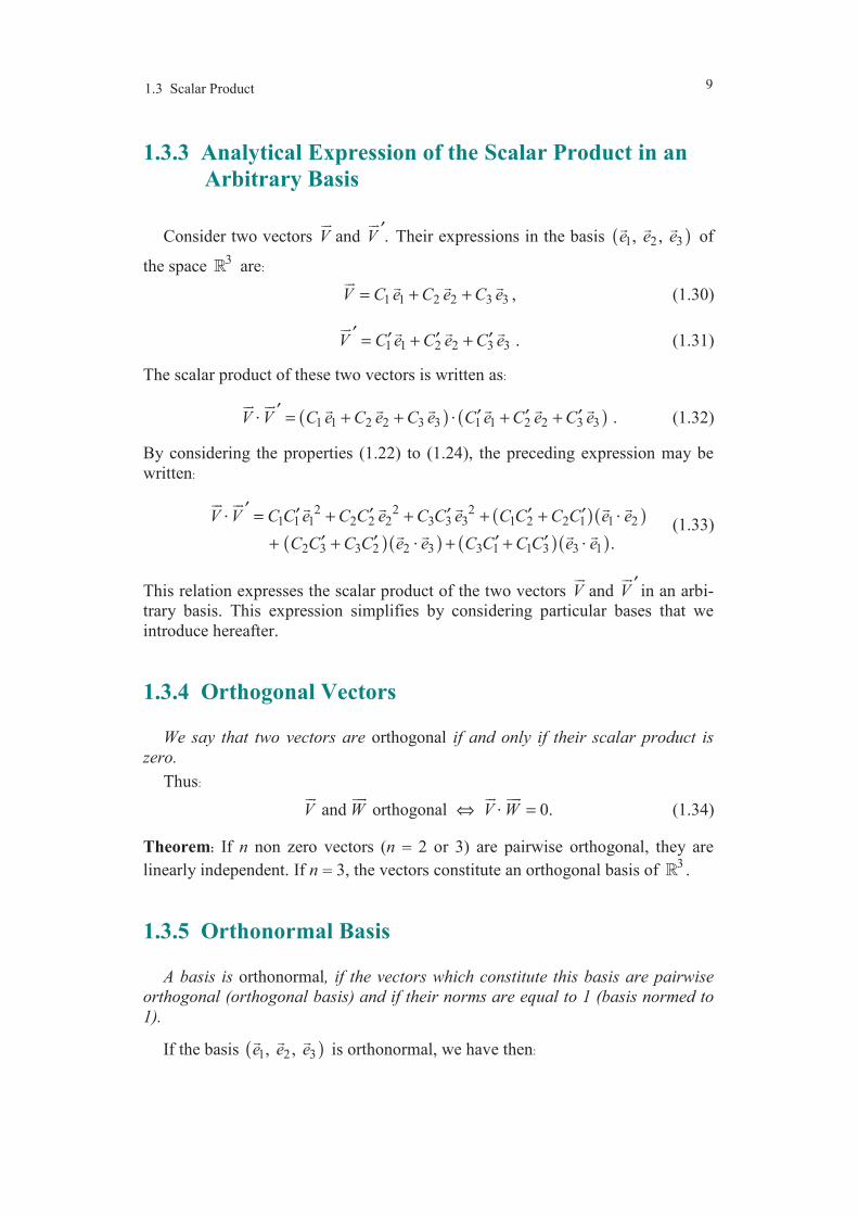
1.4.4 Expression of the Vector Product in a Direct Basis
In the case of a direct basis, Expression (1.46) of the vector product is reduced
to:
( ) ( ) ( )2 3 3 2 1 3 1 1 3 2 1 2 2 1 3V V C C C C e C C C C e C C C C e′ ′ ′ ′ ′ ′ ′= − + − + −×
. (1.48)
The preceding expression can be easily derived by expressing the vector
product in the form of a determinant (from a formalism viewpoint this writing is
however incorrect):
1 2 3
1 2 3
1 2 3
e e e
V V C C C
C C C
′ =
′ ′ ′
×
.
By expanding this determinant according to the first row, we obtain Expression
(1.48) effectively.
Furthermore, from Expression (1.48) it is easily derived that: The vector
product of V
and V ′ is a vector orthogonal to vector V
and vector .V ′
1.4.5 Mixed Product
We call mixed product of the three vectors 1 2 3, , ,V V V
considered in this
order, the real number defined by:
( )1 2 3V V V×⋅
. (1.49)
It is easy to show that, in a direct orthonormal basis, the mixed product is an
invariant in circular permutation of the three vectors.
( ) ( ) ( )1 2 3 2 3 1 3 1 2V V V V V V V V V× = × = ×⋅ ⋅ ⋅
. (1.50)
1.4.6 Property of the Double Vector Product
The double vector product of three vectors can be expressed by the relation:
( ) ( ) ( )1 2 3 1 3 2 1 2 3V V V V V V V V V× × = −⋅ ⋅
. (1.51)

1.5 Bases of the Vector Space 3 13
This equality can be easily verified by expressing the components of
( )1 2 3V V V× ×
, then the ones of ( ) ( )1 3 2 1 2 3V V V V V V−⋅ ⋅
, and then by veri-
fying that these components are equal.
1.5 BASES OF THE VECTOR SPACE R3
1.5.1 Canonical Basis
The basis of the space 3 which is the most used is the canonical basis defined
as the set of the three vectors:
( ) ( ) ( )1, 0, 0 , 0, 1, 0 , 0, 0, 1 ,i j k= = =
(1.52)
considered in this order.
We verify easily that the set ( ), , i j k
constitutes a direct orthonormal basis:
— orthonormal basis:
0, 0, 0,i j j k k i= = =⋅ ⋅ ⋅
(1.53)
2 2 21, 1, 1,i j k= = =
(1.54)
— direct basis:
, , .i j k j k i k i j× = × = × =
(1.55)
The demonstration assumes that the basis is expressed (1.52) in a basis which is
itself a direct orthonormal basis.
Afterwards, we shall denote by X, Y, Z the components of a vector V
with
respect to the canonical basis:
V X i Y j Z k= + +
. (1.56)
1.5.2 Basis Change
In this subsection, we derive, first considering an example, the relations of
basis change in the space 3 and in the case of direct orthonormal bases. Then,
the relations obtained will be generalized.
1.5.2.1 Example of a Basis Change
We consider the direct orthonormal basis ( ) ( )1 1 1 1, , b i j k=
and we derive from
this basis the set of the three vectors ( )2 2 2, , i j k
defined in the following way:
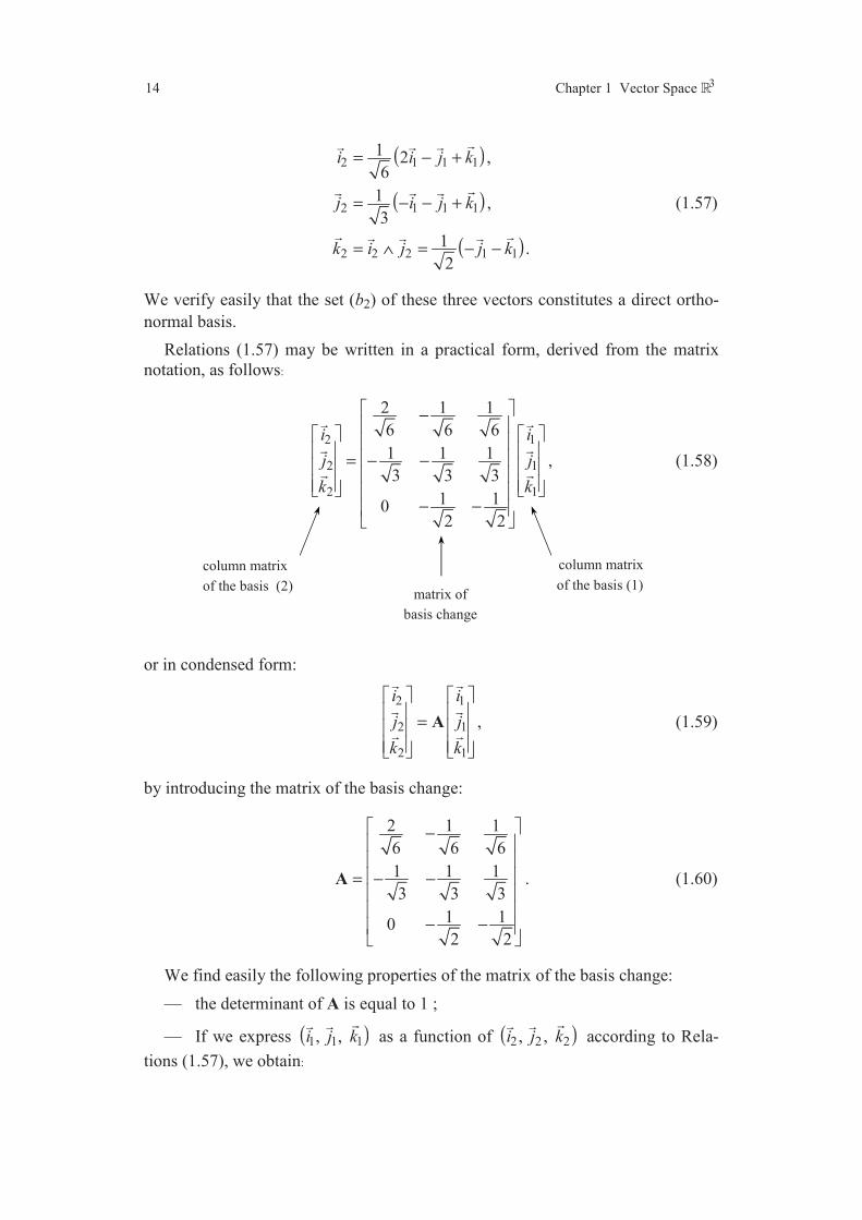
14 Chapter 1 Vector Space 3
( )
( )
( )
2 1 1 1
2 1 1 1
2 2 2 1 1
1 2 ,6
1 ,3
1 .2
i i j k
j i j k
k i j j k
= − +
= − − +
= ∧ = − −
(1.57)
We verify easily that the set (b2) of these three vectors constitutes a direct ortho-
normal basis.
Relations (1.57) may be written in a practical form, derived from the matrix
notation, as follows:
2 1
2 1
2 1
2 1 1
6 6 6
1 1 1
3 3 3
1 102 2
i i
j j
k k
− = − −
− −
, (1.58)
or in condensed form:
2 1
2 1
2 1
i i
j j
k k
=
A
, (1.59)
by introducing the matrix of the basis change:
2 1 1
6 6 6
1 1 1
3 3 3
1 102 2
− = − −
− −
A . (1.60)
We find easily the following properties of the matrix of the basis change:
— the determinant of A is equal to 1 ;
— If we express ( )1 1 1, , i j k
as a function of ( )2 2 2, , i j k
according to Rela-
tions (1.57), we obtain:
column matrix
of the basis (2) matrix of
basis change
column matrix
of the basis (1)

1.5 Bases of the Vector Space 3 15
1 2
1 2
1 2
2 1 06 3
1 1 1
6 3 2
1 1 1
6 3 2
i i
j j
k k
− = − − −
−
. (1.61)
The matrix inverse of A is equal to the matrix transposed of A:
1 t− =A A . (1.62)
Consider now the relations which exist between the components of a vector V
expressed in the two bases under consideration:
— in the basis (b1), we have:
(1) (1) (1)1 1 2 1 3 1V C i C j C k= + +
, (1.63)
— in the basis (b2), we have:
(2) (2) (2)1 2 2 2 3 2V C i C j C k= + +
, (1.64)
By substituting Relation (1.61) into Expression (1.63), we obtain:
(1) (1)1 2 2 2 2 2 2
(1)3 2 2 2
2 1 1 1 1
6 3 6 3 2
1 1 1 ,6 3 2
V C i j C i j k
C i j k
= − + − − −
+ + −
hence:
(1) (1) (1)1 2 3 2
(1) (1) (1) (1) (1)1 2 3 2 2 3 2
2 1 1
6 6 6
1 1 1 1 1 .3 3 3 2 2
V C C C i
C C C j C C k
= − +
+ − − + + − −
By comparing this result with Expression (1.64), we derive:
(2) (1) (1) (1)1 1 2 3
(2) (1) (1) (1)2 1 2 3
(2) (1) (1)3 2 3
2 1 1 ,6 6 6
1 1 1 ,3 3 3
1 1 .2 2
C C C C
C C C C
C C C
= − +
= − − +
= − −
(1.65)
By introducing the column matrices of the components in the basis (b2) and in the
basis (b1), Expression (1.65) is then written as:

16 Chapter 1 Vector Space 3
(2) (1)1 1
(2) (1)2 2
(2) (1)3 3
C C
C C
C C
=
A . (1.66)
In the same way, the inverse relation is written:
(1) (2)1 1
(1) t (2)2 2
(1) (2)3 3
C C
C C
C C
=
A . (1.67)
1.5.2.2 Generalizing
The results established in the preceding subsection for a particular case can be
generalized and expressed in the following way.
Any transformation from a direct orthonormal basis to another direct ortho-
normal basis is characterized by a square matrix, such as the determinant is equal
to 1 and the inverse matrix is the transposed matrix. Reciprocally, every matrix
which has these properties represents a change of direct orthonormal bases.
If ( )1 1 1, , i j k
and ( )2 2 2, , i j k
are two direct orthonormal bases, the basis
change is expressed in the practical form:
2 1 1 2t
2 1 1 2
2 1 1 2
, .
i i i i
j j j j
k k k k
= =
A A
(1.68)
Between the components of a vector in the two bases, we have analogous expres-
sions:
(2) (1) (1) (2)1 1 1 1
t2 2 2 2
3 3 3 3
, .
C C C C
C C C C
C C C C
= =
A A (1.69)
EXERCISES
1.1 Derive the unit vectors collinear to a given vector. Apply to the case of the
vector of components (2, –5, 3) in the canonical basis.
1.2 Determine the parameter α, in such a way as the vectors ( )1 5, 4, 3V =
and
( )2 , 2, 1V α= −
are orthogonal. The components of the vectors are given in an
orthonormal basis.
Comments 17
1.3 Derive the unit vectors orthogonal to two given vectors.
Apply to the case of the vectors of components (2, –5, 3) and (–2, 1, –3) with
respect to the canonical basis.
1.4 Expand the scalar product ( ) ( )1 2 1 2V V V V+ −⋅
; then the vector product
( ) ( )1 2 1 2V V V V+ × −
.
1.5 A vector V
has for components (4, –9, 3) in the basis ( ) ( )1 1 11 , , i j k=
. We
consider the basis ( ) ( )2 2 22 , , i j k=
deduced from (1) by the relations:
2 1 2 1 2 12 , 2 , i i j j k k= = = −
.
Express the components of V
in the basis (2).
1.6 The vectors 1V
and 2V
are two given vectors. Derive the vectors V
such as:
1 2 1V V V V× = ×
.
Apply to the case where: 1 4V i j= −
and 2 5 6 2V i j k= + −
.
COMMENTS
The vector space 3 is the space whose the vectors are characterized by
their three components which are ordered real numbers. The vector space 3 is a mathematical space with abstract feature which can not be
represented in a concrete way. However, different operations have been
defined on this space that the reader must perfectly handle: vector addition,
scalar product, vector product. The scalar product leads to the notion of
orthogonality between two vectors and the vector product to the notion of
collinear vectors. The vector space 3 is generated from a basis
×constituted of three linearly independent vectors. The basis which is the
most used is the canonical basis This basis is direct and orthonormal. Any
other direct orthonormal basis can be derived from the canonical basis
introducing a square matrix, the determinant of which is equal to 1 and the
inverse matrix is the transposed matrix.
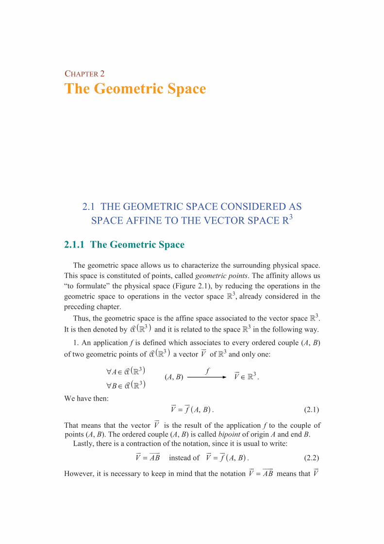
CHAPTER 2
The Geometric Space
2.1 THE GEOMETRIC SPACE CONSIDERED AS
SPACE AFFINE TO THE VECTOR SPACE R3
2.1.1 The Geometric Space
The geometric space allows us to characterize the surrounding physical space.
This space is constituted of points, called geometric points. The affinity allows us
“to formulate” the physical space (Figure 2.1), by reducing the operations in the
geometric space to operations in the vector space 3, already considered in the
preceding chapter.
Thus, the geometric space is the affine space associated to the vector space 3.
It is then denoted by ( )3 and it is related to the space 3 in the following way.
1. An application f is defined which associates to every ordered couple (A, B)
of two geometric points of ( )3 a vector V
of 3 and only one:
( )
( )
3
3
A
B
∀ ∈
∀ ∈
(A, B) 3V ∈ .
We have then:
( ),V f A B=
. (2.1)
That means that the vector V
is the result of the application f to the couple of
points (A, B). The ordered couple (A, B) is called bipoint of origin A and end B.
Lastly, there is a contraction of the notation, since it is usual to write:
V AB=
instead of ( ),V f A B=
. (2.2)
However, it is necessary to keep in mind that the notation V AB=
means that V
f
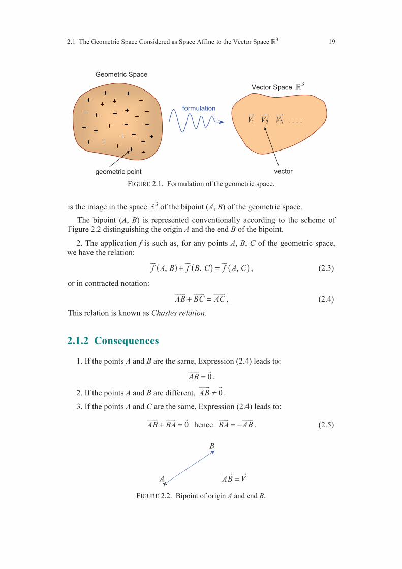
2.1 The Geometric Space Considered as Space Affine to the Vector Space 3 19
FIGURE 2.1. Formulation of the geometric space.
is the image in the space 3 of the bipoint (A, B) of the geometric space.
The bipoint (A, B) is represented conventionally according to the scheme of
Figure 2.2 distinguishing the origin A and the end B of the bipoint.
2. The application f is such as, for any points A, B, C of the geometric space,
we have the relation:
( ) ( ) ( ) , , ,f A B f B C f A C+ =
, (2.3)
or in contracted notation:
AB BC AC+ =
, (2.4)
This relation is known as Chasles relation.
2.1.2 Consequences
1. If the points A and B are the same, Expression (2.4) leads to:
0AB =
.
2. If the points A and B are different, 0AB ≠
.
3. If the points A and C are the same, Expression (2.4) leads to:
0AB BA+ =
hence BA AB= −
. (2.5)
FIGURE 2.2. Bipoint of origin A and end B.
Vector Space 3
1 2 3 . . . .V V V
formulation
Geometric Space
geometric point vector
A
B
AB V=

20 Chapter 2 The Geometric Space
4. It results that Chasles relation is written in the equivalent forms:
BC AC AB= −
, (2.6)
0AB BC CA+ + =
. (2.7)
5. Mid-point of a bipoint. The point I is the mid-point of bipoint (A, B) or seg-
ment AB if and only if:
AI IB=
. (2.8)
It results that, if O is a point of the geometric space, we have:
( )12
OI OA OB= +
. (2.9)
6. Equipollent bipoints. Two bipoints are equipollent if and only if they have
the same image in the space 3.
(A, B) equipollent to (C, D) AB CD⇔ =
. (2.10)
The quadrilateral ABCD is a parallelogram.
2.1.3 Distance between Two Points
We call distance between two points A and B or length of the segment AB, the
norm of the vector AB
.
The distance between the points A and B is denoted by d(A, B) and we have:
( )2
,d A B AB AB AB= = =
. (2.11)
The properties of the distance result from the ones of the scalar product and
norms of two vectors of 3:
— ( ), 0d A B = ⇔ A and B are the same points,
— ( ) ( ) , ,d A B d B A= ,
— ( ) ( ) ( ) , , ,d A B d A C d C B≤ + , the equality is satisfied only if the point C
is a point of the segment AB.
2.1.4 Angle between Two Bipoints
The notion of angle associated with the notion of distance allows us to localize
every point of the geometric space ( )3 .
The angle γ (Figure 2.3) between the two bipoints (A, B) and (A, C) with the
same origins and considered in this order, also called angle between the vectors
AB
and AC
, is denoted by:
( ),AB ACγ =
. (2.12)
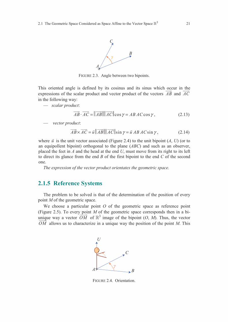
2.1 The Geometric Space Considered as Space Affine to the Vector Space 3 21
FIGURE 2.3. Angle between two bipoints.
This oriented angle is defined by its cosinus and its sinus which occur in the
expressions of the scalar product and vector product of the vectors AB
and AC
in the following way:
— scalar product:
cos cosAB AC AB AC AB ACγ γ= =⋅
, (2.13)
— vector product:
sin sinAB AC u AB AC u AB ACγ γ× = =
, (2.14)
where u
is the unit vector associated (Figure 2.4) to the unit bipoint (A, U) (or to
an equipollent bipoint) orthogonal to the plane (ABC) and such as an observer,
placed the feet in A and the head at the end U, must move from its right to its left
to direct its glance from the end B of the first bipoint to the end C of the second
one.
The expression of the vector product orientates the geometric space.
2.1.5 Reference Systems
The problem to be solved is that of the determination of the position of every
point M of the geometric space.
We choose a particular point O of the geometric space as reference point
(Figure 2.5). To every point M of the geometric space corresponds then in a bi-
unique way a vector OM
of 3 image of the bipoint (O, M). Thus, the vector
OM
allows us to characterize in a unique way the position of the point M. This
FIGURE 2.4. Orientation.
A
B
C
A B
C
U
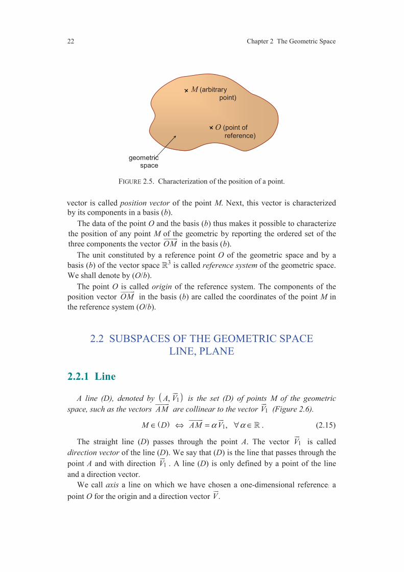
22 Chapter 2 The Geometric Space
FIGURE 2.5. Characterization of the position of a point.
vector is called position vector of the point M. Next, this vector is characterized
by its components in a basis (b).
The data of the point O and the basis (b) thus makes it possible to characterize
the position of any point M of the geometric by reporting the ordered set of the
three components the vector OM
in the basis (b).
The unit constituted by a reference point O of the geometric space and by a
basis (b) of the vector space 3 is called reference system of the geometric space.
We shall denote by (O/b).
The point O is called origin of the reference system. The components of the
position vector OM
in the basis (b) are called the coordinates of the point M in
the reference system (O/b).
2.2 SUBSPACES OF THE GEOMETRIC SPACE
LINE, PLANE
2.2.1 Line
A line (D), denoted by ( )1,A V
is the set (D) of points M of the geometric
space, such as the vectors AM
are collinear to the vector 1V
(Figure 2.6).
( ) 1 , M D AM Vα α∈ ⇔ = ∀ ∈
. (2.15)
The straight line (D) passes through the point A. The vector 1V
is called
direction vector of the line (D). We say that (D) is the line that passes through the
point A and with direction 1V
. A line (D) is only defined by a point of the line
and a direction vector.
We call axis a line on which we have chosen a one-dimensional reference: a
point O for the origin and a direction vector .V
M (arbitrary
point)
O (point of
reference)
geometric space
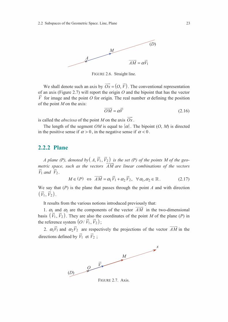
2.2 Subspaces of the Geometric Space. Line, Plane 23
FIGURE 2.6. Straight line.
We shall denote such an axis by ( ),Ox O V=
. The conventional representation
of an axis (Figure 2.7) will report the origin O and the bipoint that has the vector
V
for image and the point O for origin. The real number α defining the position
of the point M on the axis:
OM Vα=
(2.16)
is called the abscissa of the point M on the axis Ox
.
The length of the segment OM is equal to α . The bipoint (O, M) is directed
in the positive sense if 0α > , in the negative sense if 0α < .
2.2.2 Plane
A plane (P), denoted by ( ) 1 2, ,A V V
is the set (P) of the points M of the geo-
metric space, such as the vectors AM
are linear combinations of the vectors
1V
and 2 .V
( ) 1 21 2 1 2 , ,M P AM V Vα α α α∈ ⇔ = + ∀ ∈
. (2.17)
We say that (P) is the plane that passes through the point A and with direction
( )1 2,V V
.
It results from the various notions introduced previously that:
1. α1 and α2 are the components of the vector AM
in the two-dimensional
basis ( )1 2,V V
. They are also the coordinates of the point M of the plane (P) in
the reference system ( )1 2/ ,O V V
;
2. 11Vα
and 22Vα
are respectively the projections of the vector AM
in the
directions defined by 1V
et 2V
;
FIGURE 2.7. Axis.
A
(D)
M
1AM Vα=
O (D)
M
x
V

24 Chapter 2 The Geometric Space
FIGURE 2.8. Decomposition of a bipoint.
3. if we introduce the point N such as:
1 21 2, AN V NM Vα α= =
, (2.18)
Relation (2.16) is written:
AM AN NM= +
. (2.19)
Whence the construction of the point N in Figure 2.8.
The bipoint (A, N) is the projection of the bipoint (A, M) on the axis ( )1,A V
;
the bipoint (N, M) is the projection on the axis ( )2,N V
.
Generally in the construction (Figure 2.9), we introduce the projection (A, P) of
the bipoint (A, M) on the axis ( )2,A V
, bipoint of origin A and equipollent to (N,
M).
In the case where the vectors 1V
and 2V
are orthogonal, the projections consi-
dered are orthogonal projections.
2.2.3 Lines and Planes with Same Directions
2.2.3.1 Lines with Same Direction
Two lines ( )1,A V
and ( )2,B V
are of the same direction (or are parallel), if
and only if the vectors 1V
and 2V
are collinear.
FIGURE 2.9. Projections on the axes.
A
1V
M
(P) N
2V
A
1V
M
(P) N
2V
P

2.2 Subspaces of the Geometric Space. Line, Plane 25
The two lines ( )1,A V
and ( )2,B V
have the same direction if and only if:
1 2V Vλ=
or 1 2 0V V× =
. (2.20)
If the points A and B are different, the lines have no common point. If the
points A and B are the same, the two lines are identical.
2.2.3.2 Planes with Same Direction
Two planes ( ) 1 2, ,A V V
and ( ) 1 2, ,B V V′ ′ are of the same direction (or are
parallel), if and only if the vector subspaces having ( )1 2,V V
and ( )1 2,V V′ ′ for
bases are identical.
Thus, the two planes have the same direction if and only if the vectors 1V ′ and
2 ,V ′ for example, are linearly dependent on the vectors 1V
and 2 :V
1 1 2 ,1 2
2 1 21 2 .
V V V
V V V
λ λ
µ µ
′ = +
′ = +
(2.21)
If the points A and B are different, the planes have no common point. If the
points A and B are the same, the two planes are identical.
2.2.3.3 Line Parallel to a Plane
The line ( ),A V
and the plane ( ) 1 2, ,B V V
are parallel if and only if V
is
linearly dependent on 1V
and 2 ,V
hence if and only if:
1 2V V Vλ µ= +
. (2.22)
2.2.4 Orthogonal Lines and Planes
2.2.4.1 Orthogonal Lines
Two lines are orthogonal if and only if the direction vectors are orthogonal.
The line ( )1,A V
is orthogonal to the line ( )2,B V
1 2 0V V⇔ =⋅
. (2.23)
2.2.4.2 Orthogonal Lines and Planes
The line ( ),A V
is orthogonal to the plane ( ) 1 2, ,B V V
if and only if the vector
V
is orthogonal to the vector 1V
and to the vector 2V
.
Thus:
1 20, 0.V V V V= =⋅ ⋅
(2.24)

26 Chapter 2 The Geometric Space
2.2.4.3 Perpendicular Planes
Two planes are perpendicular if and only if a line of one of the planes is
orthogonal to the other plane.
2.3 CHARACTERIZATION OF THE POSITION
OF A POINT OF THE GEOMETRIC SPACE
2.3.1 Coordinate Axes
We have considered (Subsection 2.1.5) that any point M of the geometric space
could be characterized with respect to a reference system (O/b). The basis (b) is
constituted of three vectors 1 2 3, ,V V V
of the space 3, linearly independent. The
position of the point M is then characterized by the position vector OM
of the
space 3 associated to the bipoint (O, M). This vector is written:
1 2 31 2 3OM V V Vα α α= + +
. (2.25)
The parameters α1, α2, α3 are the components of the position vector OM
in the
basis ( ) 1 2 3, ,V V V
or the coordinates of the point M in the reference system
( )1 2 3/ , ,O V V V
.
The considerations developed in the previous subsections lead to the following
constructions (Figure 2.10). The reference system ( )1 2 3/ , ,O V V V
is represented
the three axes ( )1/O V
, ( )2/O V
and ( )3/O V
. On each axis, we report the
points N, P, Q with respective abscissae α1, α2, α3; hence such as:
1 2 31 2 3, , .ON V OP V OQ Vα α α= = =
(2.26)
We construct then the end R of the bipoint (N, R) equipollent to the bipoint (O,
P). From this it results:
1 21 2OR ON NR ON OP V Vα α= + = + = +
. (2.27)
Thus, the point M is the end of the bipoint (R, M) equipollent to the bipoint (O,
Q). We have well:
1 2 31 2 3OM OR RM OR OQ V V Vα α α= + = + = + +
. (2.28)
The bipoint (O, R) is the projection of the bipoint (O, M) in the plane
( )1 2/ ,O V V
. The bipoints (O, N), (O, P) and (O, Q) are the projections respect-
tively on the axes ( )1/O V
, ( )2/O V
and ( )3/O V
.
In the case where the vectors 1V
, 2V
and 3V
are orthogonal, the projections are
orthogonal projections.

2.3 Characterization of a Point of the Geometric Space 27
FIGURE 2.10. Projections of a point.
2.3.2 Direct Orthonormal Reference System
The reference system ( )1 2 3/ , ,O V V V
is a direct orthonormal reference system
if the vectors 1 2 3, ,V V V
constitute a direct orthonormal basis.
We have then:
1. 2 2 2
1 2 31, 1, 1.V V V= = =
The vectors are unit vectors.
2. 1 2 2 3 3 10, 0, 0V V V V V V⋅ = ⋅ = ⋅ =
. The axes ( )1/O V
, ( )2/O V
and
( )3/O V
are pairwise orthogonal. We say that the set of the three axes is a tri-
rectangular system.
3. 1 2 3 2 3 1 3 1 2, , V V V V V V V V V× = × = × =
. The system is oriented in
the direct sense: an observer, placed the feet at the point O and the head at the end
of the axis 3O
, must move from its right to its left to direct its glance from the
end of the 1-axis to the end of the 2-axis (Figure 2.11). The orientation of the
system is unchanged in a circular permutation of the indexes. It is also said that
the reference system is a right-handed system.
2.3.3 Cartesian Coordinates
The reference systems used are usually direct orthonormal reference systems
of which the basis is the canonical basis of the space 3, hence:
1 2 3, , V i V j V k= = =
. (2.29)
In the following, the axes will be denoted by:
( ) ( ) ( ) , , , , , ,Ox O i Oy O j Oz O k= = =
(2.30)
O
1V
M
N
2V
P
3V
R
Q

28 Chapter 2 The Geometric Space
FIGURE 2.11. Direct or right-handed system.
and the reference system is denoted by:
( ) ( ) / , ,Oxyz O i j k=
. (2.31)
The points N, P, Q (Figure 2.12) considered in the subsection 2.3.1 have
respective abscissae on the axes which are denoted by x, y, z and are called
Cartesian coordinates of the point M.
The vector image of the bipoint (O, M) is written:
OM x i y j z k= + +
. (2.32)
The Cartesian coordinates of the point M are the components, in the canonical
basis of 3, of the vector .OM
FIGURE 2.12. Cartesian system.
3V
O 1V
2V
1
2
3
left
right
2
1
O
i
j
k
x
y
z
Q
P
R N
M

2.4 Plane and Line Equations 29
2.4 PLANE AND LINE EQUATIONS
2.4.1 Cartesian Equation of a Plane
We are searching for the Cartesian equation of the plane ( ) 1 2, ,A V V
:
— passing through the point A of Cartesian coordinates xA, yA, zA with respect
to the Cartesian system ( ) / , ,O i j k
;
— of direction defined by the vectors 1V
and 2V
of respective components
(X1, Y1, Z1) and (X2, Y2, Z2) in the canonical basis ( ) , ,i j k
.
Thus, we have:
1 1 1 1
2 2 2 2
,
,
.
A A AOA x i y j z k
V X i Y j Z k
V X i Y j Z k
= + +
= + +
= + +
(2.33)
The plane ( ) 1 2, ,A V V
is the set of the points M such as:
1 21 2 1 2, ,AM V Vα α α α= + ∀ ∈
. (2.34)
The Cartesian equation of the plane is the relation which allows us to express
the Cartesian coordinates (x, y, z) of the point M:
OM x i y j z k= + +
. (2.35)
By expressing the vector AM
, we have:
( ) ( ) ( )A A AAM OM OA x x i y y j z z k= − = − + − + −
. (2.36)
By substituting then this expression into (2.34), and then by equating the respec-
tive components for i
, j
and k
, we obtain:
1 1 2 2
1 1 2 2
1 1 2 2
,
,
.
A
A
A
x x X X
y y Y Y
z z Z Z
α α
α α
α α
− = +
− = +
− = +
(2.37)
These equations are the parametric equations of the plane.
The Cartesian equation is obtained by eliminating the parameters α1 and α2.
Thus:
( )( ) ( ) ( ) ( )( )1 2 1 2 1 2 1 2 1 2 1 2 0A A AZ Y Y Z x x X Z Z X y y Y X X Y z z− − + − − + − − = .
(2.38)
The Cartesian equation of a plane is then of the form:
1 2 1 2 1 2 1 2
1 2 1 2
0,
with
, ,
, .A A A
ax by cz d
a Z Y Y Z b X Z Z X
c Y X X Y d ax by cz
+ + + =
= − = −
= − = − − −
(2.39)

30 Chapter 2 The Geometric Space
Plane passing through three non-aligned points
To find the equation of the plane passing through the points A, B, C of res-
pective coordinates (xA, yA, zA ), (xB, yB, zB), (xC, yC, zC), we search for the plane
passing through the point A and of direction defined, for example, by the vectors
AC
and AB
:
( ) ( ) ( )
( ) ( ) ( )
1
2
,
.
C A C A C A
B A B A B A
V AC x x i y y j z z k
V AB x x i y y j z z k
→ = − + − + −
→ = − + − + −
(2.40)
By substituting the components of these vectors into Equation (2.38), we obtain
the equation of the plane.
Particular planes
— Plane ( ) ( ) , ,Oxy O i j=
: the vectors 1V
and 2V
are the vectors i
and .j
The
vector equation of the plane is written:
1 2 1 2, ,x i y j z k i jα α α α+ + = + ∀ ∈
, (2.41)
and the parametric equations are:
1 2 1 2, , 0, ,x y zα α α α= = = ∀ ∈ . (2.42)
— We find analogous equations for the planes (Oyz) and (Oxz).
2.4.2 Cartesian Equations of a Line
We search for the equation of the line ( )1,A V
passing through the point A and
of direction 1.V
With notations already used, the vector equation (2.15) leads to
the three parametric equations:
1
1
1
,
,
.
A
A
A
x x X
y y Y
z z Z
α
α
α
− =
− =
− =
(2.43)
If 1 1 1, and X Y Z are non zero, these equations lead to one of the following pairs of
equations:
( ) ( ) ( )
( ) ( ) ( )
1 1 1
1 1 1
1 1 1
1 1 1
, , ,
, , ,
A A A A A A
A A A A A A
Y Z Xy y x x z z y y x x z z
X Y Z
Z X Xz z x x x x y y y y z z
X Y Z
− = − − = − − = −
− = − − = − − = −
(2.44)
equations which may be written in the form:
1 1 1
AA Ay yx x z z
X Y Z
−− −= = . (2.45)
A line is then defined by two Cartesian equations.

2.5 Change of Reference System 31
O11i
1j1k
y1
z1 M
x1
z2
y2
O2
x2
2j
2i
2k
Particular cases
— If X1 = 0, the equations of the line are:
( )1
1
0,
.
A
A A
x x
Yy y z z
Z
− =
− = − (2.46)
This is the equation of a line contained in the plane Ax x= .
— We obtain similar equations in the case of lines contained in the plane
1 ( 0)Ay y Y= = or in the plane 1 ( 0)Az z Z= = .
2.5 CHANGE OF REFERENCE SYSTEM
In this section we consider only the case of direct orthonormal reference
systems.
2.5.1 General Case
We consider two reference systems (Figure 2.13):
( ) ( ) ( )
( ) ( ) ( )
1 1 1 1 1 1 1 1 1
2 2 2 2 2 2 2 2 2
/ , , ,
/ , , .
T O x y z O i j k
T O x y z O i j k
= =
= =
The problem to be solved is:
Starting from the coordinates with respect to the reference system (T2) of a
point M of the geometric space, we have to find the coordinates of M expressed
with respect to the reference system (T1).
FIGURE 2.13 Change of reference system .
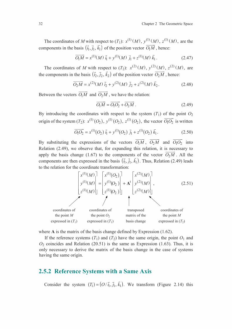
32 Chapter 2 The Geometric Space
The coordinates of M with respect to (T1): ( ) ( ) ( )(1) (1) (1), , ,x M y M z M are the
components in the basis ( ) 1 1 1, ,i j k
of the position vector 1O M
, hence:
( ) ( ) ( )(1) (1) (1)1 1 1 1O M x M i y M j z M k= + +
. (2.47)
The coordinates of M with respect to (T2): ( ) ( ) ( )(2) (2) (2), , ,x M y M z M are
the components in the basis ( ) 2 2 2, ,i j k
of the position vector 2O M
, hence:
( ) ( ) ( )(2) (2) (2)2 2 2 2O M x M i y M j z M k= + +
. (2.48)
Between the vectors 1O M
and 2O M
, we have the relation:
1 1 2 2O M O O O M= +
. (2.49)
By introducing the coordinates with respect to the system (T1) of the point O2
origin of the system (T2): ( ) ( ) ( )(1) (1) (1)2 2 2, , ,x O y O z O the vector 1 2O O
is written
( ) ( ) ( )(1) (1) (1)1 2 2 1 2 1 2 1O O x O i y O j z O k= + +
. (2.50)
By substituting the expressions of the vectors 1O M
, 2O M
and 1 2O O
into
Relation (2.49), we observe that, for expanding this relation, it is necessary to
apply the basis change (1.67) to the components of the vector 2O M
. All the
components are then expressed in the basis ( ) 1 1 1, ,i j k
. Thus, Relation (2.49) leads
to the relation for the coordinate transformation:
( )
( )
( )
( )
( )
( )
( )
( )
( )
(1) (1) (2)2
(1) (1) t (2)2
(1) (1) (2)2
x M x O x M
y M y O y M
z M z O z M
= +
A , (2.51)
coordinates of coordinates of transposed coordinates of
the point M the point O2 matrix of the the point M
expressed in (T1) expressed in (T1) basis change expressed in (T2)
where A is the matrix of the basis change defined by Expression (1.62).
If the reference systems (T1) and (T2) have the same origin, the point O1 and
O2 coincides and Relation (20.51) is the same as Expression (1.63). Thus, it is
only necessary to derive the matrix of the basis change in the case of systems
having the same origin.
2.5.2 Reference Systems with a Same Axis
Consider the system ( ) ( ) 1 1 1 1/ , , .T O i j k=
We transform (Figure 2.14) this
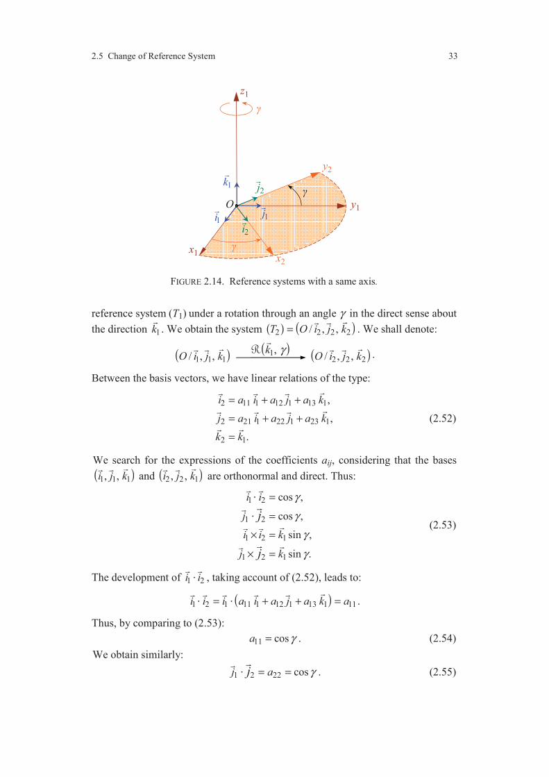
2.5 Change of Reference System 33
FIGURE 2.14. Reference systems with a same axis.
reference system (T1) under a rotation through an angle γ in the direct sense about
the direction 1k
. We obtain the system ( ) ( ) 2 2 2 2/ , ,T O i j k=
. We shall denote:
( ) 1 1 1/ , ,O i j k
( ) 2 2 2/ , ,O i j k
.
Between the basis vectors, we have linear relations of the type:
2 11 1 12 1 13 1
2 21 1 22 1 23 1
2 1
,
,
.
i a i a j a k
j a i a j a k
k k
= + +
= + +
=
(2.52)
We search for the expressions of the coefficients aij, considering that the bases
( ) 1 1 1, ,i j k
and ( ) 2 2 1, ,i j k
are orthonormal and direct. Thus:
1 2
1 2
1 2 1
1 2 1
cos ,
cos ,
sin ,
sin .
i i
j
i i k
j k
j
j
γ
γ
γ
γ
=
=
× =
× =
⋅
⋅
(2.53)
The development of 1 2i i⋅
, taking account of (2.52), leads to:
( ) 1 2 1 11 1 12 1 13 1 11i i i a i a j a k a= + + =⋅ ⋅
.
Thus, by comparing to (2.53):
11 cosa γ= . (2.54)
We obtain similarly:
1 2 22 cosj aj γ= =⋅
. (2.55)
O
1i
1k
y1
z1
x1
y2
x2
2j
( )1,k γ
1j
2i
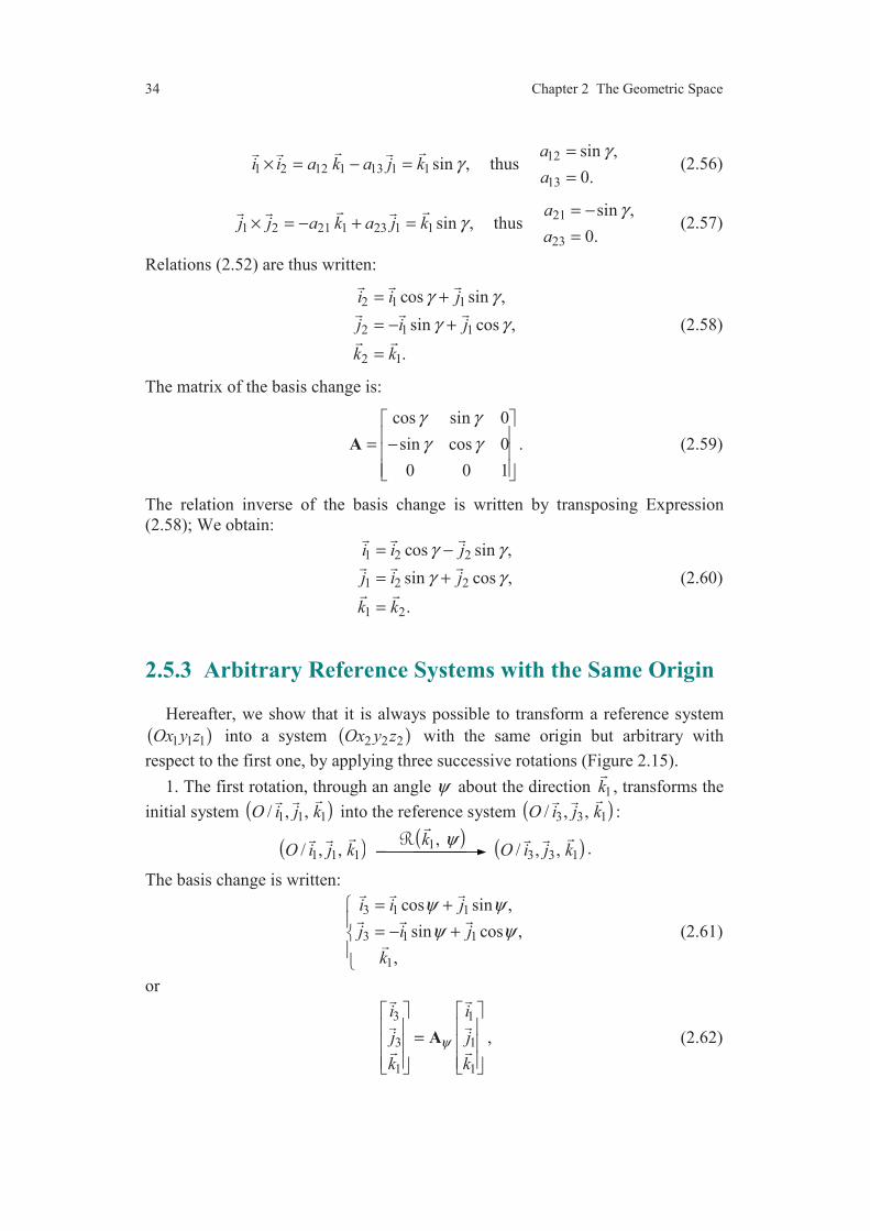
34 Chapter 2 The Geometric Space
12
1 2 12 1 13 1 113
sin ,sin , thus
0.
ai i a k a j k
a
γγ
=× = − =
=
(2.56)
21
1 2 21 1 23 1 123
sin ,sin , thus
0.
aj j a k a j k
a
γγ
= −× = − + =
=
(2.57)
Relations (2.52) are thus written:
2 1 1
2 1 1
2 1
cos sin ,
sin cos ,
.
i i j
j i j
k k
γ γ
γ γ
= +
= − +
=
(2.58)
The matrix of the basis change is:
cos sin 0
sin cos 0
0 0 1
γ γ
γ γ
= −
A . (2.59)
The relation inverse of the basis change is written by transposing Expression
(2.58); We obtain:
1 2 2
1 2 2
1 2
cos sin ,
sin cos ,
.
i i j
j i j
k k
γ γ
γ γ
= −
= +
=
(2.60)
2.5.3 Arbitrary Reference Systems with the Same Origin
Hereafter, we show that it is always possible to transform a reference system
( )1 1 1Ox y z into a system ( )2 2 2Ox y z with the same origin but arbitrary with
respect to the first one, by applying three successive rotations (Figure 2.15).
1. The first rotation, through an angle ψ about the direction 1k
, transforms the
initial system ( ) 1 1 1/ , ,O i j k
into the reference system ( ) 3 3 1/ , ,O i j k
:
( ) 1 1 1/ , ,O i j k
( ) 3 3 1/ , ,O i j k
.
The basis change is written:
3 1 1
3 1 1
1
cos sin ,
sin cos ,
,
i i j
j i j
k
ψ ψ
ψ ψ
= +
= − +
(2.61)
or
3 1
3 1
1 1
i i
j j
k k
ψ
=
A
, (2.62)
( )1,k ψ
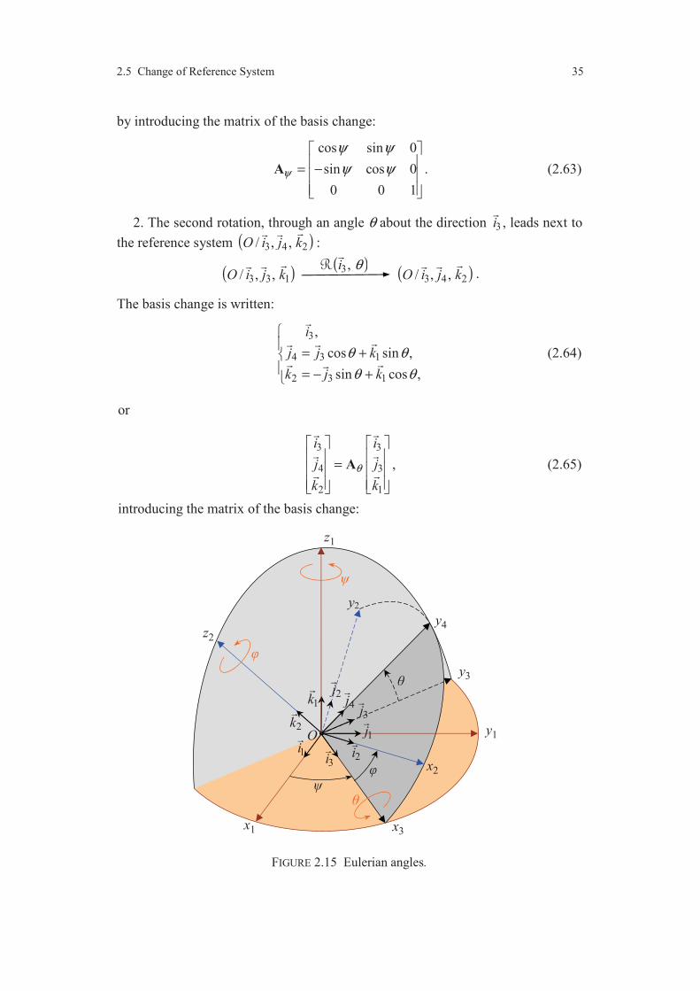
2.5 Change of Reference System 35
by introducing the matrix of the basis change:
cos sin 0
sin cos 0
0 0 1
ψ
ψ ψ
ψ ψ
= −
A . (2.63)
2. The second rotation, through an angle θ about the direction 3i
, leads next to
the reference system ( ) 3 4 2/ , ,O i j k
:
( ) 3 3 1/ , ,O i j k
( ) 3 4 2/ , ,O i j k
.
The basis change is written:
3
4 3 1
2 3 1
,
cos sin ,
sin cos ,
i
j j k
k j k
θ θ
θ θ
= + = − +
(2.64)
or
3 3
4 3
2 1
i i
j j
k k
θ
=
A
, (2.65)
introducing the matrix of the basis change:
FIGURE 2.15 Eulerian angles.
( )3,i θ
z1
x1
O1i
1k
y1
y3
3j
3i
x3
1j
2k
2i
4j
x2
2j
y4
y2
z2
36 Chapter 2 The Geometric Space
1 0 0
0 cos sin
0 sin cos
θ θ θ
θ θ
= −
A . (2.66)
The system ( )3 4 2Ox y z is not arbitrary with respect to the first one, since the axis
3Ox
is contained in the plane ( )1 1Ox y of the first system. So, it is necessary to
consider a third rotation to obtain an arbitrary system.
3. The third rotation, through an angle ϕ around the direction 2 ,k
leads to the
second system ( )2 2 2 ,Ox y z which is arbitrary with respect to the first one:
( ) 3 4 2/ , ,O i j k
( ) 2 2 2/ , ,O i j k
.
The basis change is written:
2 3 4
2 3 4
2
cos sin ,
sin cos ,
,
i i j
j i j
k
ϕ ϕ
ϕ ϕ
= +
= − +
(2.67)
or
2 3
2 4
2 2
i i
j j
k k
ϕ
=
A
, (2.68)
by introducing the matrix of the basis change:
cos sin 0
sin cos 0
0 0 1
ϕ
ϕ ϕ
ϕ ϕ
= −
A . (2.69)
The three rotation angles then introduced are called the Eulerian angles: ψ is the
precession angle, θ the nutation angle, ϕ is the proper rotation angle or the spin
angle. They completely characterize the situation of the second system.
The relation of the basis change which expresses ( ) 2 2 2, ,i j k
as a function of
( ) 1 1 1, ,i j k
introduces the matrix A of basis change:
2 1
2 1
2 1
i i
j j
k k
=
A
. (2.70)
This relation can be obtained by combining Relations (2.61), (2.64) and (2.67).
So, this relation is deduced from the matrix (2.62), (2.65) and (2.68). Indeed, we
may write from these relations:
2 3 3 1
2 4 3 1
2 2 1 1
( ) ( ( ))
i i i i
j j j j
k k k k
ϕ ϕ θ ϕ θ ψ
= = =
A A A A A A
,
( )2 ,k ϕ

Exercises 37
or by taking into account the associativity of the matrix product:
( )2 1
2 1
2 1
i i
j j
k k
ϕ θ ψ
=
A A A
. (2.71)
The comparison between relations (2.70) and (2.71) leads to:
ϕ θ ψ=A A A A . (2.72)
The matrix of the basis change is equal to the product of the three matrices in the
order: 3rd rotation, 2nd rotation, 1st rotation. Calculation leads to:
cos cos sin cos sin sin cos cos cos sin sin sin
cos sin sin cos cos sin sin cos cos cos sin cos
sin sin cos sin cos
ψ ϕ ψ θ ϕ ψ ϕ ψ θ ϕ θ ϕ
ψ ϕ ψ θ ϕ ψ ϕ ψ θ ϕ θ ϕ
ψ θ ψ θ θ
− +
= − − − +
−
A .
(2.73)
EXERCISES
2.1 Derive the coordinates of the orthogonal projection H of a point M on the line
(D) (Figure 2.16). The coordinates x, y, z of the point M are given and the line (D)
passes through the origin point O and has V
for direction vector.
Apply the result to the case where the direction vector V
has (1, –2, 3) for
components in the canonical basis.
2.2 Derive the equation of the line passing through the point A (–1, 2, 1) and or-
thogonal to the plane passing through the three points A, B (2, 3, –1), C (–3, 4, –2).
2.3 Show that the triangle having for vertices the points of Cartesian coordinates:
( ) ( ) ( ) 2, 0, 2 , 1, 2, 1 , 1, 2, 1 ,A B C− − − −
is an isoscele triangle rectangular at A.
FIGURE 2.16. Orthogonal projection of a point on a line.
M (x, y, z)
H
OV
(D)

38 Chapter 2 The Geometric Space
FIGURE 2.17. Parallelepiped.
2.4 Derive the area of the triangle ABC, the vertices of which have the Cartesian
coordinates:
A (–1, –2, –1) , B (2, 2, –1) , C (3, 2, 1) .
2.5 Calculate the volume of a parallelepiped (Figure 2.17), constructed on the
bipoints (A, B), (A, C) and (A, D).
Apply the result to the case of the points of Cartesian coordinates:
A (0, 0, 0) , B (3, 2, 1) , C (1, 1, 2) , D (–1, –1, 2) .
2.6 Calculate the distance from the point D to the plane that passes (Figure 2.18)
through three points A, B and C.
Apply the results to the case where the Cartesian coordinates are:
A (0, 0, 0) , B (1, 2, 3) , C (2, 1, 1) , D (–2, –1, –3) .
2.7 Find the necessary and sufficient condition for which the four points A, B, C
and D are contained in the same plane.
2.8 We consider a direct orthonormal system ( ) ( ) 1 1 1 1/ , ,T O i j k=
. This system is
transformed using a rotation through an angle of 30° around the axis ( )1,O i
: we
obtain the system ( ) 1 3 2/ , ,O i j k
. Next, we apply to this new system a rotation
FIGURE 2.18. Distance from a point to a plane.
AB
C
D
H
A B
C
D

Comments 39
through an angle of 45° around the axis ( )2,O k
: we obtain the reference system
( ) ( ) 2 2 2 2/ , ,T O i j k=
.
1. Derive the relations which express the basis vectors ( ) 2 2 2, ,i j k
of the
system ( )2T as functions of the basis vectors ( ) 1 1 1, ,i j k
of the system ( )1T .
2. A point M has for Cartesian coordinates (–1, 2, 4) with respect to the system
( )1 1 1Ox y z . Derive the Cartesian coordinates with respect to the system ( )2 2 2Ox y z .
3. A point N has for Cartesian coordinates (3, –4, 8) with respect to the system
( )2 2 2Ox y z . Derive the coordinates with respect to the system ( )1 1 1Ox y z .
COMMENTS
The notion of geometric space allows us to characterize the surrounding
physical space. This space is then a concrete space constituted of geometric
points, and its formulation is obtained by reducing the operations in the
geometric space to operations in the vector space 3, operations introduced
in the previous chapter.
An arbitrary solid of the geometric space is defined by the set of its
points of which the positions are determined by their coordinates. The
coordinates that are the most used are the Cartesian coordinates defined
with respect to a Cartesian reference system constituted of an origin O and
three tri-rectangular axes Ox
, Oy
and Oz
, with unit direction vectors
, and ,i j k
the vectors of the canonical basis. When the set of the coordi-
nates of the points of the solid are obtained, all information about the solid
is known and the figure can be deleted. Next, all the properties or
transformations of the solid are obtained from operations in the vector
space 3, implemented on the image vectors of the bipoints of the solid.

CHAPTER 3
Vector FunctionDerivatives of a Vector Function
3.1 VECTOR FUNCTION OF ONE VARIABLE
3.1.1 Definition
If, to any value of a real variable q, there corresponds a vector ,V
then V
is
called a vector function of the scalar variable q.
We shall denote such a function by ( )V q
:
q ∈ ( ) 3V q ∈
. (3.1)
If the vector ( )V q
is defined by its components in a given basis, these compo-
nents are real functions of the variable q. The vector function will be then deter-
mined by reporting the three components of the ( )V q
: X(q), Y(q), Z(q), for
example in the basis ( ) ( ) 1 2 3, ,b e e e=
:
1 2 3( ) ( ) ( ) ( )V q X q e Y q e Z q e= + +
. (3.2)
3.1.2 Derivative
The first derivative of the vector function ( )V q
with respect to the variable q
and in the basis ( ) ( ) 1 2 3, ,b e e e=
, that we shall denote by:
( )dd
b
Vq
or
( )dd
b Vq
, (3.3)
is defined by:

3.1 Vector Function of One Variable 41
( )
1 2 3d d d dd d d d
b X Y ZV e e eq q q q
= + +
. (3.4)
In the problems where only one basis is considered, the vector obtained is simply
called the derivative vector of ( )V q
with respect to q and it will be denoted by
ddVq
. Thus, it is implied that the derivative is concerned in the considered basis. In
the case where several bases are considered (case of the Mechanics of Solids), it is
necessary to specify the basis in which the derivation is implemented.
For example, if the vector ( )V q
is defined:
— in the basis ( ) ( ) 1 1 11 , ,i j k=
by:
(1) (1) (1)1 1 1( ) ( ) ( ) ( )V q i X q j Y q k Z q= + +
, (3.5)
— in the basis ( ) ( ) 2 2 22 , ,i j k=
by:
(2) (2) (2)2 2 2( ) ( ) ( ) ( )V q i X q j Y q k Z q= + +
, (3.6)
we shall distinguish:
— the vector (1)d
dV
q
, derivative of V
in the basis (1):
(1) (1) (1) (1)
1 1 1d d d dd d d d
X Y ZV i j kq q q q
= + +
, (3.7)
— and the vector (2)d
dV
q
, derivative of V
in the basis (2):
(2) (2) (2) (2)
2 2 2d d d dd d d d
X Y ZV i j kq q q q
= + +
. (3.8)
Generally, these two vectors are different.
3.1.3 Properties of the Vector Derivative
If the vectors ( ) ( ) ( )1 2 3, et V q V q V q
are vector functions of the same variable
q, we have in a given basis:
1. ( )
1 21 2
d ddd d d
V VV V
q q q+ = +
. (3.9)
This relation can be extended to the case of an arbitrary number of vectors.
2. ( )
1 21 2 2 1
d ddd d d
V VV V V V
q q q= +⋅ ⋅ ⋅
, (3.10)
42 Chapter 3 Vector Function. Derivatives of a Vector Function
with in particular:
2d d2d d
VV Vq q
= ⋅
. (3.11)
3. ( )
1 21 2 2 1
d ddd d d
V VV V V V
q q q× = × + ×
. (3.12)
4. ( ) ( )
31 21 2 3 2 3 1 3 1 2
dd ddd d d d
VV VV V V V V V V V V
q q q q
× = × + × + ×
⋅ ⋅ ⋅ ⋅
.
(3.13)
5. If f(q) is a real function of the variable q:
( )
dd dd d d
f Vf V V fq q q
= +
. (3.14)
In particular, if ( )f q k= independent of q:
( )
d dd d
VkV kq q
=
. (3.15)
6. If q is a function of the variable p: q(p)
dd dd d d
qV Vp q p
=
. (3.16)
7. The differential of the vector function V
is defined as:
dd dd d dd d d
qV VV q pq q p
= =
. (3.17)
As the derivative, the differential depends on the basis under consideration.
3.1.4 Examples
3.1.4.1 First Example
We consider, in the basis ( ) ( ) 1 , ,i j k=
, the vector:
( ) cos sinu i jα α α= +
. (3.18)
The derivative with respect to α in the basis (1) is:
(1)d ( ) sin cos cos ( ) sin ( )d 2 2
u i j i jπ πα α α α αα
= − + = + + +
.
Whence the important relation:
(1)d ( ) ( )d 2
u u πα αα
= +
. (3.19)
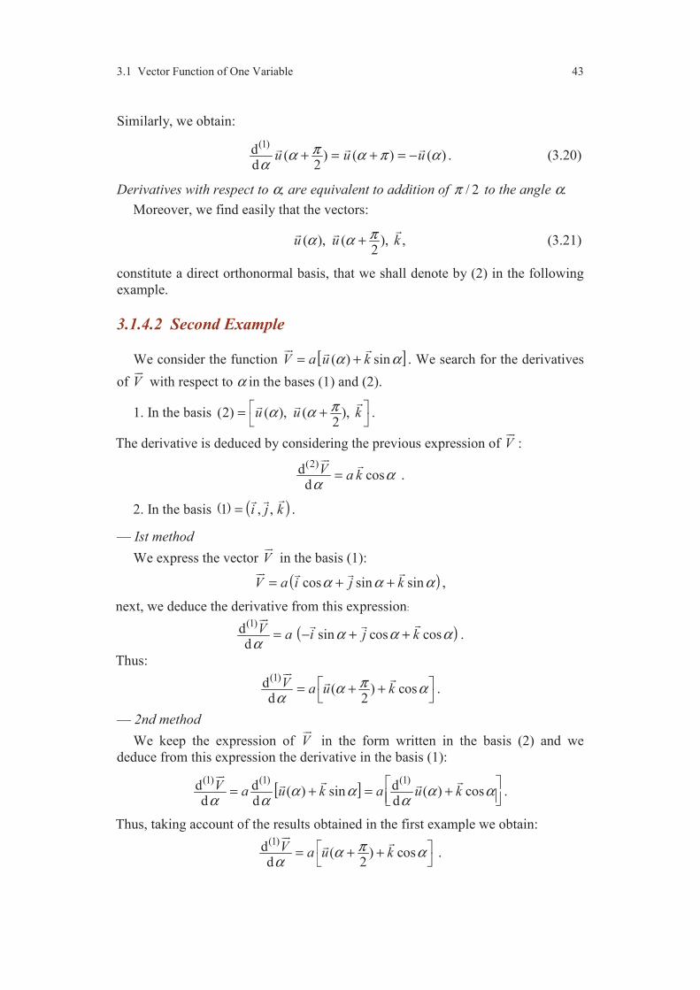
3.1 Vector Function of One Variable 43
Similarly, we obtain:
(1)d ( ) ( ) ( )d 2
u u uπα α π αα
+ = + = −
. (3.20)
Derivatives with respect to α, are equivalent to addition of / 2π to the angle α.
Moreover, we find easily that the vectors:
( ), ( ), ,2
u u kπα α +
(3.21)
constitute a direct orthonormal basis, that we shall denote by (2) in the following
example.
3.1.4.2 Second Example
We consider the function [ ]( ) sinV a u kα α= +
. We search for the derivatives
of V
with respect to α in the bases (1) and (2).
1. In the basis (2) ( ), ( ), 2
u u kπα α = +
.
The derivative is deduced by considering the previous expression of V
:
(2)d cosd
V a k αα
=
.
2. In the basis ( ) ( ) 1 , ,i j k=
.
— Ist method
We express the vector V
in the basis (1):
( )cos sin sinV a i j kα α α= + +
,
next, we deduce the derivative from this expression:
( )(1)d sin cos cosd
V a i j kα α αα
= − + +
.
Thus: (1)d ( ) cosd 2
V a u kπα αα
= + +
.
— 2nd method
We keep the expression of V
in the form written in the basis (2) and we
deduce from this expression the derivative in the basis (1):
[ ]
(1) (1) (1)d d d( ) sin ( ) cosd d d
V a u k a u kα α α αα α α
= + = +
.
Thus, taking account of the results obtained in the first example we obtain: (1)d ( ) cosd 2
V a u kπα αα
= + +
.

44 Chapter 3 Vector Function. Derivatives of a Vector Function
3.1.4.3 Third Example
Obtain the derivative of 2cos sin 2V a i b j c kα α= + +
with respect to α in
the basis ( ) , ,i j k
, where a, b and c are real number independent of α.
The derivative is easily obtained as:
d 2 cos sin 2 cos 2d
V a i b jα α αα
= − +
.
3.2 VECTOR FUNCTION OF TWO VARIABLES
3.2.1 Definition
If, to any pair of two real independent variables q1 and q2, there corresponds a
vector ,V
then V
is called a vector function of the scalar variables q1 and q2.
We denote such a function by 1 2( , )V q q
. The components of this vector are
functions of q1 and q2, and in the basis ( ) ( ) 1 2 3, , ,b e e e=
we have:
1 2 1 2 1 1 2 2 1 2 3( , ) ( , ) ( , ) ( , )V q q X q q e Y q q e Z q q e= + +
. (3.22)
3.2.2 Partial Derivatives
The partial derivatives of the function 1 2( , )V q q
in the basis (b) are defined as
follows:
— derivative with respect to q1 :
( )
1 2 31 1 1 1
b V X Y Ze e eq q q q
∂ ∂ ∂ ∂= + +∂ ∂ ∂ ∂
, (3.23)
— derivative with respect to q2 :
( )
1 2 32 2 2 2
b V X Y Ze e eq q q q
∂ ∂ ∂ ∂= + +∂ ∂ ∂ ∂
. (3.24)
When only one basis is considered, the partial derivatives are simply denoted
by 1
Vq
∂∂
and 2
Vq
∂∂
.
The differential of the vector function 1 2( , )V q q
is defined by:
( ) ( )( )
1 21 2
d d db b
b V VV q qq q
∂ ∂= +∂ ∂
. (3.25)

3.2 Vector Function of n Variables 45
If q1 and q2 are functions of the same variable p, the derivative of V
with respect
to p is given by:
( ) ( ) ( )1 2
1 2
d ddd d d
b b bq qV V Vp q p q p
∂ ∂= +∂ ∂
. (3.26)
3.2.3 Examples
Obtain the partial derivatives and the differential in the basis ( ) , ,i j k
of the
function:
( ) 2 2
1 2 1 1 2 1 2( , ) 2V q q a q i q q j q q k = + + +
.
We obtain easily:
( ) ( )
( ) ( )
1 2 1 21 2
1 2 1 1 2 2
2 2 , 2 ,
d 2 2 d 2 d .
V Va q i q j k a q j q kq q
V a q i q j k q q j q k q
∂ ∂= + + = +∂ ∂
= + + + +
3.3 VECTOR FUNCTION OF n VARIABLES
3.3.1 Definitions
The previous considerations can be extended to the case of an arbitrary number
of variables.
A vector function of the variables 1 2, , . . . , nq q q , associates to any set of the
values of these n variables a vector denoted by 1 2( , , . . . , )nV q q q
.
The components of the vector 1 2( , , . . . , )nV q q q
are real functions of the n
variables, and in the basis ( ) ( ) 1 2 3, , ,b e e e=
we have:
1 2 1 2 1 1 2 2 1 2 3( , , . . . , ) ( , , . . . , ) ( , , . . . , ) ( , , . . . , ) .n n n nV q q q X q q q e Y q q q e Z q q q e= + +
(3.27)
The partial derivative of the function V
with respect to the variable qi
( 1, 2, . . . , )i n= in the basis (b) is defined by:
( )
1 2 3
b
i i i i
V X Y Ze e eq q q q
∂ ∂ ∂ ∂= + +∂ ∂ ∂ ∂
, (3.28)
and the differential of V
in the basis (b) is written:
( )( )
1
d d
n bb
ii
i
VV qq
=
∂=∂
. (3.29)

46 Chapter 3 Vector Function. Derivatives of a Vector Function
If 1 2, , . . . , nq q q are functions of the same variable p, the derivative of V
with
respect to p in the basis (b) is:
( ) ( )
1
ddd d
nb bi
ii
qV Vp q p
=
∂=∂
. (3.30)
3.3.2 Examples
3.3.2.1 Example 1. Cylindrical Coordinates
Let M be a point of the geometric space localized by its Cartesian coordinates
(x, y, z). The position vector of the point M is:
OM x i y j z k= + +
. (3.31)
The position of the point M can be also characterized (Figure 3.1) by the para-
meters:
( ), , , -abscissa of ,r OH i OH z z Mα= = =
(3.32)
where H is the orthogonal projection of the point M in the plane (Oxy). The
position parameters (r, α, z) are called the cylindical coordinates of the point M.
The position vector (3.31) is then written:
cos sinOM r i r j z kα α= + +
,
or
( )OM r u z kα= +
. (3.33)
This is the expression of the position vector, when the point M is localized by its
cylindrical coordinates.
FIGURE 3.1. Cylindrical coordinates.
k
O
i
j
x
y
z
z
H x
M
( )u α
( )2
u πα +
y
r

3.2 Vector Function of n Variables 47
The vector ( )u α
(3.18) is the unit direction vector of the line OH. Similarly,
the vector ( )2
u πα +
is the unit direction vector of the line orthogonal to OH
(Figure 3.1). The system ( )/ ( ), ( ), 2
O u u kπα α +
is a direct orthonormal system.
Consider the partial derivatives of the position vector OM
with respect to r, α,
z, in the basis ( ) , ,i j k
. We have:
( ), ( ), ,2
OM OM OMu r u kr k
πα αα
∂ ∂ ∂= = + =∂ ∂ ∂
and the differential of the position vector is written:
d ( ) d ( ) d d2
OM u r r u k zπα α α= + + +
. (3.34)
If for example r, α and z are functions of the time t, the derivative with respect
to t in the basis ( ) , ,i j k
is the velocity vector of the point M with respect to the
reference system (T) = (Oxyz) and is written according to (3.30):
( )( ) d d d d( , ) ( ) ( )
d d d 2 d
TT OM r zM t u r u k
t t t tα πα α= = + + +
. (3.35)
The components of the velocity vector in the basis ( ), ( ), 2
u u kπα α +
are then:
( )
d d d, , d d d
r zrt t t
α . (3.36)
3.3.2.2 Example 2. Basis Change
Let ( ) 1 1 1, ,i j k
and ( ) 2 2 2, ,i j k
be two bases, of which the transformation from
one basis to the other is obtained by using the Eulerian angles (ψ, θ, ϕ). We wish
to express the partial derivatives, in the basis (1) and with respect to ψ, θ and ϕ, of
the vectors 2 2 2, ,i j k
. In this way, we consider again the three rotations introduced
in Subsection 2.5.3.
— 1st rotation
( ) 1 1 1/ , ,O i j k
( ) 3 3 1/ , ,O i j k
.
We have:
3 1 1
3 1 1
( ) cos sin ,
( ) sin cos .2
i u i j
j u i j
ψ ψ ψ
πψ ψ ψ
= = +
= + = − +
Whence
(1) (1)3 3
3 3, .i j
j iψ ψ
∂ ∂= = −
∂ ∂
(3.37)
( )1,k ψ

48 Chapter 3 Vector Function. Derivatives of a Vector Function
— 2nd rotation
( ) 3 3 1/ , ,O i j k
( ) 3 4 2/ , ,O i j k
.
We have:
4 3 1
2 3 1
( ) cos sin ,
( ) sin cos .2
j u j k
k u j k
θ θ θ
πθ θ θ
= = +
= + = − +
From this we deduce: (1) (1)
4 43 2
(1) (1)2 2
3 4
cos , ,
sin , .
j ji k
k ki j
θψ θ
θψ θ
∂ ∂= − =
∂ ∂
∂ ∂= = −
∂ ∂
(3.38)
— 3rd rotation
( ) 3 4 2/ , ,O i j k
( ) 2 2 2/ , ,O i j k
.
We have:
2 3 4
2 3 4
( ) cos sin ,
( ) sin cos .2
i u i j
j u i j
ϕ ϕ ϕ
πϕ ϕ ϕ
= = +
= + = − +
Whence the searched results:
(1) (1) (1)2 2 2
3 3 2 2
(1) (1) (1)2 2 2
3 3 2 2
(1) (1) (1)2 2 2
3 4
cos cos sin , sin , ,
sin cos cos , cos , ,
sin , , 0.
i i ij i k j
j j jj i k i
k k ki j
ϕ θ ϕ ϕψ θ ϕ
ϕ θ ϕ ϕψ θ ϕ
θψ θ ϕ
∂ ∂ ∂= − = =
∂ ∂ ∂
∂ ∂ ∂= − − = = −
∂ ∂ ∂
∂ ∂ ∂= = − =
∂ ∂ ∂
(3.39)
It follows from this that the differential in the basis (1) of 2i
is written:
( )
(1)2 3 3 2 2d cos cos sin d sin d di j i k jϕ θ ϕ ψ ϕ θ ϕ= − + +
, (3.40)
or
( )
(1)2 1 3 2 2d d d di k i k iψ θ ϕ= + + ×
. (3.41)
If the angles ψ, θ, ϕ (and consequently the vectors 2 2 2, ,i j k
) depend on the
variable p, we may write:
(1)2
2d
dp
ii
pω= ×
, (3.42)
by introducing:
1 3 2d ddd d d
p k i kp p p
ψ ϕθω = + +
. (3.43)
( )3,i θ
( )2 ,k ϕ

Comments 49
Similarly, we find:
(1) (1)2 2
2 2d d
, .d d
p pj k
j kp p
ω ω= × = ×
(3.44)
Important application
We seek for the expression of the derivative with respect to the variable p and
in the basis (1) of a vector V
whose components in the basis (2) are independent
of the parameter p , for example, the position vector of a point fixed in the
reference system ( ) 2 2 2/ , ,O i j k
. We have:
(2) (2) (2)2 2 2V X i Y j Z k= + +
, (3.45)
where the components X(2), Y(2), and Z(2) are independent of parameter p. The
derivative in the basis (1) of the vector V
is written:
(1)(1) (1)(1)(2) (2) (2)22 2dd dd
d d d d
ji kV X Y Zp p p p
= + +
, (3.46)
hence from (3.42) and 3.44):
( )
(1)(2) (2) (2)
2 2 2d
dp
V X i Y j Z kp
ω= × + +
. (3.47)
Whence the result: (1)dd
pV V
pω= ×
. (3.48)
This result will be used in Kinematics of Rigid Body (Chapter 9).
COMMENTS
The concepts of derivatives will be used in Kinematics (Part II). We
will have to express the velocity vectors and acceleration vectors of the
points of a rigid body. These vectors will be deduced from the derivatives
of the position vectors with respect to the time and in different reference
systems, that will lead to consider the derivatives in different bases. The
notions developed in Subsections 3.1, 3.2 and 3.3 must thus be perfectly
assimilated. The examples considered in this chapter are sufficient to illus-
trate the use of the vector derivatives.
The result (3.48) of Subsection 3.3.2.2 is an important result that will be
used in Kinematics of Rigid Body (Chapter 9). This result is interesting
owing to the fact that the derivative operation is replaced by a vector
product that is easier to implement, in particular in the case of a numerical
application.
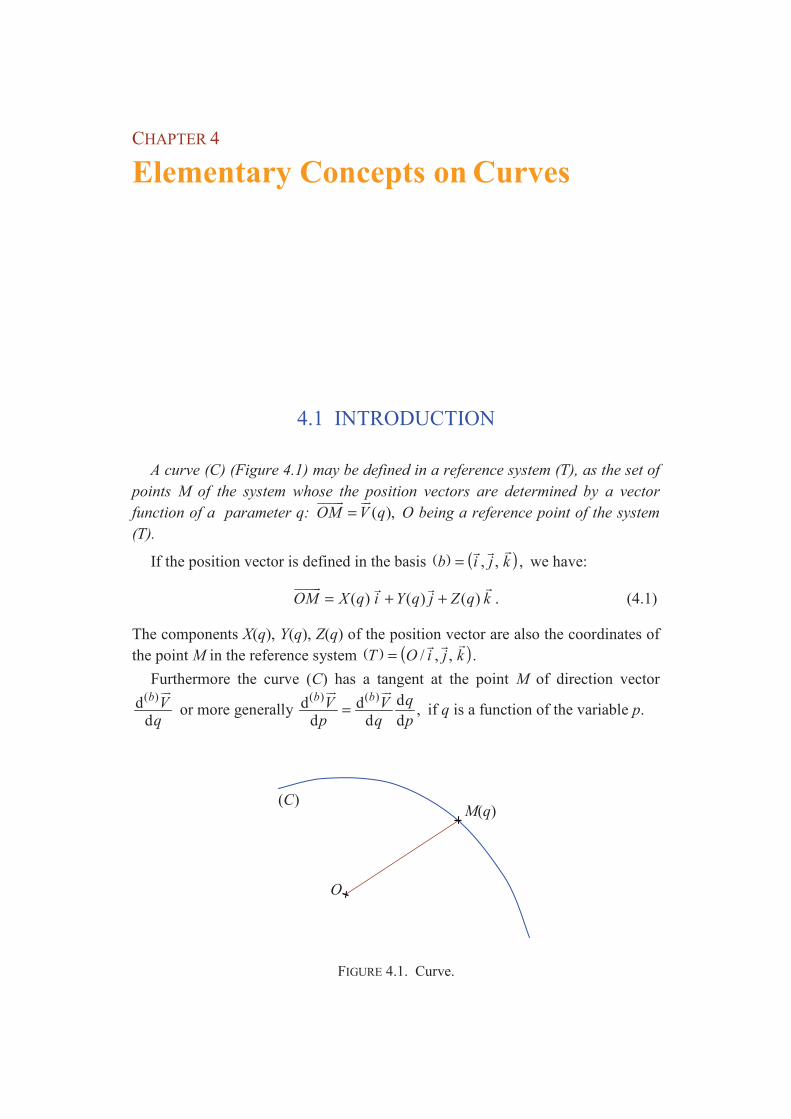
CHAPTER 4
Elementary Concepts on Curves
4.1 INTRODUCTION
A curve (C) (Figure 4.1) may be defined in a reference system (T), as the set of
points M of the system whose the position vectors are determined by a vector
function of a parameter q: ( ),OM V q=
O being a reference point of the system
(T).
If the position vector is defined in the basis ( ) ( ) , , ,b i j k=
we have:
( ) ( ) ( )OM X q i Y q j Z q k= + +
. (4.1)
The components X(q), Y(q), Z(q) of the position vector are also the coordinates of
the point M in the reference system ( ) ( ) / , , .T O i j k=
Furthermore the curve (C) has a tangent at the point M of direction vector ( )dd
b Vq
or more generally
( ) ( ) dd d ,d d d
b b qV Vp q p
=
if q is a function of the variable p.
FIGURE 4.1. Curve.
O
M(q) (C)

4.2 Curvilinear Abscissa. Arc Length of a Curve 51
4.2 CURVILINEAR ABSCISSA
ARC LENGTH OF A CURVE
Among all the variables q which allow us to characterize the position of the
point M on the curve (C), a particular variable has been chosen, which will be
denoted by s, such as the vector ( )d
d
b OMs
is a unit vector:
2( ) ( )d d1 or 1d d
b bOM OMs s
= =
. (4.2)
Let M ′ be a point infinitely close to the point M (Figure 4.2) obtained by
increasing the variable s by the value d .s We have:
( )( ) dd d
d
bb OMMM OM OM OM s
s′ ′= − = =
. (4.3)
The arc length of the curve between the two points and M M ′ is the same as the
length MM ′ . Thus:
( ) ( )d dd dd d
b bOM OMMM MM s ss s
′ ′≈ = = ±
. (4.4)
Whence the result:
ds MM ′= ± . (4.5)
If M0 and M are two arbitrary points of the curve (C), the previous relation is
written as:
0 0( ) ( )s M s M M M− = ± . (4.6)
The variable s thus introduced measures the arc length of the curve. Its sign
depends on the orientation of the curve. We shall write for example:
0( ) ( )s M s M− = . (4.7)
The curve is thus oriented in the sense of the increase of s. The variable s is called
the curvilinear abscissa of the point M.
FIGURE 4.2. Arc length.
M0M
O
( )M s(C)
( d )M s s′ +
M0
52 Chapter 4 Elementary Concepts on Curves
If the point M0 is taken as the origin of the curvilinear abscissae, it follows
from this that: 0( ) 0,s M = and Relation (4.6) is written:
0( )s M M M= ± . (4.8)
4.3 TANGENT. NORMAL. RADIUS OF CURVATURE
From the definition of the curvilinear abscissa, it follows that the vector:
( )dd
b
tOMes
=
(4.9)
is a unit vector. The vector te
is thus the unit direction vector of the tangent to the
curve (C) at the point M, orientated in the sense of the increasing s. The orientated
tangent is the axis ( ), tM e
.
Since 2 1te =
, we obtain by considering the derivative of this expression with
respect to s and in the basis (b):
( )d0
d
bt
te
es
=⋅
. (4.10)
The vector ( )d
d
bte
s
is thus orthogonal to the vector te
, and we state:
( )d
d
bt ne e
s=
, (4.11)
where by definition:
— ne
is the unit vector of the principal normal direction of the curve (C) at
the point M ;
— is a positive scalar called the radius of curvature of the curve (C) at the
point M.
4.4 FRENET TRIHEDRON
The two vectors te
and ne
constitute the first two vectors of a direct ortho-
normal basis. The third vector, called the unit vector of the binormal direction of
the curve (C) at the point M, is defined by the relation:
b t ne e e= ×
. (4.12)
The basis thus obtained is called the basis of Frenet. It is a function of the
curvilinear abscissa s, hence of the point M. The moving reference system (Figure
4.3) ( )/ , , t n bM e e e
is called the Frenet trihedron.

4.4 Frenet Trihedron 53
FIGURE 4.3. Frenet trihedron.
The plane ( )/ ,t nM e e
is the osculating plane at M of the curve (C), the plane
( )/ ,n bM e e
is the normal plane at M of the curve (C), and the plane ( )/ ,b tM e e
is the rectifying plane at M of the curve (C).
The derivative of the position vector OM
with respect to the parameter q and
in the basis (b) is written:
d d d dd d d d
tOM OM s se
q s q q= =
. (4.13)
And considering the second derivative, we obtain:
( )
22 2 2
2 2 2
d dd d d d dd d d dd d d
t tt t
e eOM s s s se eq q s qq q q
= + = +
, (4.14)
or taking account of (4.11):
( )
22 2
2 2
d d ddd d
nt
eOM s seqq q
= +
. (4.15)
From this relation, it follows that:
1. The bipoint of origin M and image 2
2
d
d
OM
q
is contained in the osculating
plane of the curve (C) at M (Figure 4.4).
2. The scalar product:
( )22
2
d 1 ddd
nOM se
qq=⋅
, (4.16)
is always positive. The vector 2
2
d
d
OM
q
has thus always a positive component
in the direction defined by ne
and this component defines the convexity of
the curve (C) at the point M.
Lastly, the point D defined by:
nMD e=
(4.17)
is called the centre of curvature of the curve (C) at the point M (Figure 4.4).
te
M
(C)
be
ne

54 Chapter 4 Elementary Concepts on Curves
FIGURE 4.4. Convexity and curvature.
EXERCISE
4.1 In the reference system ( ) / , ,O i j k
, we define the curve (C) as the set of the
points M of Cartesian coordinates:
3 3sin , cos , cos 2 ,x a q y a q z a q= = = − with 0 and 02
a q π> < < .
Derive the unit direction vector of the tangent, the curvilinear abscissa, the
vector of the principal normal, the radius of curvature and the basis of Frenet at an
arbitrary point of the curve (C).
COMMENTS
The present chapter introduces the elementary concepts relative to the space
curves. Exercise 4.1 illustrates how these concepts can be used simply
starting from their definitions.
te
M
(C)
be
ne
Dosculating plane
normalplane
ddOM
q
2
2
d
d
OM
q
CHAPTER 5
Torsors
5.1 DEFINITION AND PROPERTIES OF THE TORSORS
5.1.1 Definitions and Notations
A torsor, which we shall denote by may be defined as the set of two fields
of vectors, defined on the geometric space or on a subspace (D) of the geometric
space and having the following properties.
1. The first field of vectors associates to every point P of the space (D) a vector
R
of 3, independent of the point under consideration:
( )P D∀ ∈ 3R ∈ . (5.1)
The vector R
is called the resultant of the torsor . We shall denote this
resultant by R
or .R
2. The second field of vectors associates to every point P of the space (D) a
vector P
which depends on the point P:
( )P D∀ ∈ 3P ∈
. (5.2)
The vector P
is called the moment vector at the point P or moment at the
point P of the torsor . We will denote the moment by P
or P
.
Between the moment vectors at two points P and Q of the space (D), there
exists the relation:
Q P R PQ= + × . (5.3)
This fundamental relation can be considered as the relation of definition of the
field of moment vectors, and by extension as the relation of definition of the
torsors:
The torsor is the set of the two fields of vectors: resultant and moment
56 Chapter 5 Torsors
defined on the space (D), satisfying Relation (5.3) at every point P of this space.
The two vectors R
and P
are called the elements of reduction at the point P
of the torsor or the vector components at the point P of the torsor .
Usually, we shall denote these elements by , P PR . The importance of the
elements of reduction at a point results from the following theorem:
If R
and P
are two given vectors, and if P is a given point, there exists one
torsor and only one having R
and P
as elements of reduction at P. From this
theorem, it results that a torsor is defined in a unique way if the elements of
reduction are given at a point.
The six real numbers X, Y, Z and LP, MP, NP, respective components of R
and
P
in a given basis, are called the components at P of the torsor . Usually,
we shall denote these components by , , , , , P P P PX Y Z L M N .
5.1.2 Properties of the Moments
The two moment vectors P
at the point P and Q
at the point Q have the
same projection on the line PQ: we say that the field of the moment vectors is
equiprojective.
The projection of the moment vector P
on PQ (or more generally along the
direction PQ
) is given according to the definition by the scalar product PPQ ⋅
(except for a multiplicative factor). Considering Expression (5.3), we may write:
( )Q PPQ PQ PQ R PQ= + ×⋅ ⋅ ⋅ . (5.4)
The two vectors PQ
and R PQ×
being orthogonal, the previous relation is redu-
ced to:
Q PPQ PQ=⋅ ⋅ . (5.5)
This relation expresses that the vectors P
and Q
have the same projection
on the line PQ.
5.1.3 Vector Space of Torsors
The set of the torsors defined on a space (D) constitutes a vector space.
5.1.3.1 Equality of Two Torsors
Two torsors are equal (we say also equivalent), if and only if there exists a
5.1 Definition and Properties of the Torsors 57
point at which the elements of reduction of the two torsors are equal.
The equality between two torsors:
1 2= (5.6)
is thus equivalent to the set of the two vector equalities:
1 2
1 2
,
and for example .P P
R R =
=
(5.7)
5.1.3.2 Sum of Two Torsors
The torsor sum of the two torsors 1 and 2 , which we shall denote by:
1 2= + (5.8)
has for elements of reduction at a point P:
1 2
1 2
,
.P P P
R R R = +
= +
(5.9)
5.1.3.3 Multiplication by a Scalar
The torsor:
1λ= , (5.10)
where λ is a real number, has for elements of reduction at a point P:
1
1
,
.P P
R Rλ
λ
=
=
(5.11)
5.1.3.4 Null Torsor
The null torsor or zero torsor, denoted by ,0 is the neutral element for the
addition of the two torsors. Its elements of reduction at any point are:
( )
0,
0, .
0
0P
R
P D
=
= ∀ ∈
(5.12)
5.1.4 Scalar Invariant of a Torsor
The scalar invariant of a torsor is by definition the scalar product of the
elements of reduction at an arbitrary point of the torsor under consideration.
The scalar invariant is independent of the point chosen, that justifies the inte-
rest of the definition. Indeed, if we consider the torsor , the scalar invariant
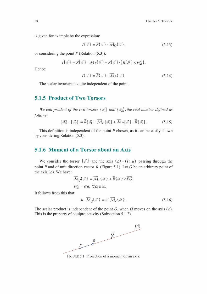
58 Chapter 5 Torsors
is given for example by the expression:
QI R= ⋅
, (5.13)
or considering the point P (Relation (5.3)):
( )PI R R R PQ= + ×⋅ ⋅
.
Hence:
PI R= ⋅
. (5.14)
The scalar invariant is quite independent of the point.
5.1.5 Product of Two Torsors
We call product of the two torsors 1 and 2 , the real number defined as
follows:
1 2 1 2 1 2P PR R= +⋅ ⋅ ⋅
. (5.15)
This definition is independent of the point P chosen, as it can be easily shown
by considering Relation (5.3).
5.1.6 Moment of a Torsor about an Axis
We consider the torsor and the axis ( ) ( ), P u∆ =
passing through the
point P and of unit direction vector u
(Figure 5.1). Let Q be an arbitrary point of
the axis (∆). We have:
,
, .
Q P R PQ
PQ uα α
= + ×
= ∀ ∈
It follows from this that:
Q Pu u=⋅ ⋅ . (5.16)
The scalar product is independent of the point Q, when Q moves on the axis (∆).
This is the property of equiprojectivity (Subsection 5.1.2).
FIGURE 5.1 Projection of a moment on an axis.
P
()
Q
u

5.1 Definition and Properties of the Torsors 59
The scalar product Pu ⋅ is called the moment of the torsor about
the axis ( ), P u
. It is independent of the point chosen on the axis.
Note. Not to confuse:
— the moment of a torsor about an axis which is a real number ;
— and the moment of a torsor at a point which is a vector.
5.1.7 Central Axis of a Torsor
We consider a given torsor with a nonzero resultant. The set of the points of the
geometric space at which the moment of the torsor is collinear to its resultant is a
line which has this resultant as direction vector. This line is called the central axis
of the torsor.
Thus:
Central axis of the torsor ( ), PP Rα α= = ∀ ∈
. (5.17)
Let us show this theorem. Let be then a given torsor and we search for the
set (∆) of the points P such as P
is collinear to ,R
or what is equi-
valent such as:
0PR × = . (5.18)
Let O be a reference point of the geometric space. Expression (5.3) is written:
P O R OP= + × . (5.19)
The condition (5.18) of collinearity is then written:
( ) 0OR R R OP× + × × = , (5.20)
or taking account of the property (1.51) of the double vector product:
( ) 20OR R OP R R OP× + − =⋅
. (5.21)
From this expression, we derive:
2 2OR R OP
OP RR R
×= +
⋅
. (5.22)
The first term is a vector independent of the point P:
0 2OR
VR
×=
. (5.23)
The second term depends on the point P, and we introduce the real number λdepending on the point P:
2
R OP
Rλ =
⋅
(5.24)
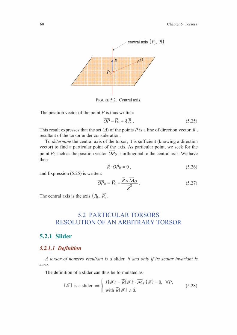
60 Chapter 5 Torsors
FIGURE 5.2. Central axis.
The position vector of the point P is thus written:
0OP V Rλ= +
. (5.25)
This result expresses that the set (∆) of the points P is a line of direction vector R
,
resultant of the torsor under consideration.
To determine the central axis of the torsor, it is sufficient (knowing a direction
vector) to find a particular point of the axis. As particular point, we seek for the
point P0 such as the position vector 0OP
is orthogonal to the central axis. We have
then:
0 0R OP =⋅
, (5.26)
and Expression (5.25) is written:
0 0 2OR
OP VR
×= =
. (5.27)
The central axis is the axis ( )0 , P R
.
5.2 PARTICULAR TORSORS
RESOLUTION OF AN ARBITRARY TORSOR
5.2.1 Slider
5.2.1.1 Definition
A torsor of nonzero resultant is a slider, if and only if its scalar invariant is
zero.
The definition of a slider can thus be formulated as:
is a slider ⇔
0, ,
with 0.
PI R P
R
= = ∀
≠
⋅
(5.28)
P0
central axis ( )0 , P R
O R
5.2 Particular Torsors. Resolution of an Arbitrary Torsor 61
The scalar invariant being independent of the point P at which it is determined,
it is equivalent to say:
A torsor is a slider if and only if there exists at least a point at which the
moment of the torsor is zero.
5.2.1.2 Moment at a Point of a Slider
We consider the slider . There exists at least a point at which the moment
of the slider is zero. Let A be this point:
0A = . (5.29)
The moment at an arbitrary point P is written:
P A R AP= + × . (5.30)
Hence:
P R AP= × . (5.31)
This relation expresses the moment vector at an arbitrary point P of a slider of
which the moment is zero at the point A.
5.2.1.3 Axis of a Slider
Let be a slider and A a point at which the moment of the torsor is zero.
We search for the set of the points P at which the moment of the slider is zero.
From (5.31) the set of these points satisfies the relation:
0 with 0R AP R× = ≠ . (5.32)
This relation shows that AP
is collinear to the resultant, hence the point P is a
point of the line passing through the point A and which has the resultant of the
slider as direction vector.
This line is called the axis of the null moments of the slider or in a contracted
state: the axis of the slider. This axis is the central axis of the slider.
5.2.1.4 Conclusions
1. A torsor , of nonzero resultant, is a slider if and only if the scalar inva-
riant is zero.
2. A slider is entirely determined when are given:
— its resultant: ,R
— a point A at which its moment is null: 0A = .
3. A slider has an axis of null moments: the axis ( ), A R .
4. If Q is an arbitrary point of this axis, the moment at the arbitrary P is
expressed as:
P R QP= × . (5.33)

62 Chapter 5 Torsors
5.2.2 Couple-Torsor
5.2.2.1 Definition
A nonzero torsor is a couple-torsor if and only if the resultant of this torsor is
zero.
Hence:
is a couple-torsor
0,
a point such as 0.P
R
P
=⇔
∃ ≠
(5.34)
5.2.2.2 Property of the Moment-Vector
It follows from Expression (5.3) that a couple-torsor is such as:
P Q= = , (5.35)
where is a vector independent of the points P and Q.
The moment-vector is independent of the point under consideration.
5.2.2.3 Resolution of a Couple-Torsor
Let c be a couple-torsor 0, . This couple-torsor can be resolved into
the sum of two sliders 1 and 2 :
1 2 c = + , (5.36)
where the sliders are defined as follows:
1 2
1 2
1 2
0,
, being an arbitrary point,
0, 0.
P P
R R
P
I I
+ =
+ = = =
(5.37)
The first relation shows that there exists an infinity of couples of sliders equi-
valent to a given couple-torsor. The sliders which constitute one of these have
opposite resultants. Thus, the axes of the sliders are parallel.
One of these equivalent couples can be obtained in the following way.
1. We choose the slider 1 while giving us:
— its resultant 11R R= ;
— its axis (∆1) determined by a point P1: ( ) ( )11 1, P R∆ =
.
At this stage there is thus a “double” infinity of possible choices. When these
choices are done, the resolution is unique.
5.2 Particular Torsors. Resolution of an Arbitrary Torsor 63
2. The slider 2 is then defined as follows:
— its resultant is 12R R= − ;
— its axis (∆2) is determined, if we know one of the points of this axis: P2 for
example. The point P2 is such as:
2 2 21 2 1P P P+ = = . (5.38)
Whence from (5.33):
1 1 2R P P× =
. (5.39)
This relation determines the point P2 in a unique way.
5.2.3 Arbitrary Torsor
5.2.3.1 Définition
A torsor is arbitrary if and only if its scalar invariant is nonzero.
is an arbitrary torsor 0I⇔ ≠ . (5.40)
5.2.3.2 Resolution of an Arbitrary Torsor
An arbitrary torsor can be resolved into a sum of a slider and a couple-torsor;
and this by an infinity in ways.
The resolution of an arbitrary torsor is implemented as follows.
1. We choose a point P where the elements of reduction of the torsor are
known, thus:
and .PR (5.41)
There is an infinity of possible choices for the point P. This choice will depend
on the easiness to express the elements of reduction of the torsor at such or such
point. Once the choice of P made, the resolution of the torsor is unique.
2. The slider 1 is such as:
— its resultant is equal to the resultant of the torsor :
1 ,R R=
(5.42)
— its axis passes through the point P chosen.
3. the couple-torsor 2 is such as:
2 20, .PR = =

64 Chapter 5 Torsors
We obtain well thus:
1 2= + . (5.44)
At each point P chosen is associated a couple: slider/couple-torsor, and only
one. The sliders of all the couples equivalent to a given arbitrary torsor have the
same resultant. They differ by their axes which have however the same direction,
given by the resultant of the torsor.
5.2.4 Conclusions
Let be a torsor of elements of reduction at P: R and .P
1. If 0PI R= =⋅
1.1 If 0R ≠ , the torsor is a slider.
1.2 If 0R =
— If 0 P P= ∀ , the torsor is the null torsor.
— If 0P ≠ , the torsor is a couple-torsor, which may be resolved into a
sum of two sliders of opposite resultants.
2. If 0PI R= ≠⋅
, the torsor is an arbitrary torsor. The torsor
may be resolved, at a point P, into a slider of resultant R and of axis
( ), P R and a couple-torsor of moment vector .P
5.3 TORSORS ASSOCIATED TO A FIELD
OF SLIDERS DEFINED ON A
DOMAIN OF THE GEOMETRIC SPACE
Afterwards, we shall be brought to consider torsors associated to fields of
torsors defined on particular subspaces of the geometric space: for example, the
set of the points of a rigid body, the set of the points of several bodies, etc. We
shall note (D) this subspace which could be a curve, an area or a volume.
Moreover, this domain could be finite (if there exist a one-to-one mapping of the
points onto the natural numbers), or infinite otherwise.
5.3.1 Torsor Associated to a Finite Set of Points
Let us consider a finite set (D) = (M1, M2, . . . , Mi, . . . , Mn) constituted of n
points. On this domain (D) we define a field of sliders which associates to each

5.3 Torsors Associated to a Field of Sliders Defined on a Domain of the Geometric Space 65
point Mi of the domain (D) a slider i of axis passing through the point Mi:
( )iM D∀ ∈ .i (5.45)
The torsor i is a slider of resultant iR
and axis passing through Mi:
, 1, 2, . . . , .
0,i
ii
M i
R Ri n
==
=
(5.46)
We call torsor associated to the domain (D) and to the field of sliders i
defined on (D), the torsor ( ) D sum of the sliders i . Whence:
( ) 1
n
i
i
D
=
= . (5.47)
It follows from this definition that:
— the resultant of the torsor ( ) D is:
( ) 1 1
n n
ii
i i
R D R R
= =
= =
, (5.48)
— the moment at an arbitrary point P of the geometric space of the torsor
( ) D is given by the expression:
( ) 1 1
n n
i iP P i
i i
D PM R
= =
= = × . (5.49)
5.3.2 Torsors Associated to an Infinite Set of Points
Let (D) be an infinite domain of the geometric space (Figure 5.3). On this
domain (D), we consider a field of sliders which associates to every point M of the
domain (D) a slider, denoted by ( ) d M , of axis passing through M, defined in
the following way:
( )M D∀ ∈ ( ) d .M (5.50)
The torsor ( ) d M is a slider of resultant d ( )R M
and axis passing though M:
( )
( )
d d ( ),
d 0.M
R M R M
M
=
=
(5.51)
The resultant d ( )R M
may be put in the form:
d ( ) ( ) d ( )R M R M e M=
, (5.52)

66 Chapter 5 Torsors
FIGURE 5.3. Infinite domain.
where d ( )e M is an element of the domain (D) surrounding the point M: element
of curve, area or volume, according as the domain is a curve, an area or a volume.
The vector ( )R M
is called the vector density of the field of sliders. The torsor
associated to the field of sliders (5.50) is derived as an extension to an infinite
domain of Expressions (5.47) to (5.49).
The torsor associated to the domain (D) and to the field of sliders ( ) d M
defined on (D) is the torsor ( ) D that we admit to write:
( ) ( ) ( )
dD
D M= . (5.53)
It follows from this expression and by extension of (5.48) and (5.49) that:
— the resultant of the torsor ( ) D is:
( )
( ) ( )
d ( ) ( ) d ( )D D
R D R M R M e M= = , (5.54)
— the moment at the arbitrary point P of the geometric space of the torsor
( ) D is expressed as:
( )
( ) ( )
d ( ) ( ) d ( )PD D
D PM R M PM R M e M= × = × . (5.55)
The integrals which occur in the preceding expressions will be curve, area or
volume integrals according to the nature of the domain (D): curve, area or
volume.
Relations (5.54) and (5.55) are well suited to a method of literal calculation of
the integrals. However, it is always possible to reduce the case of an infinite
domain to the case of a finite domain. In this way, the domain (D) is divided into
n elements (Figure 5.4). The element (i) is then referred by the point Mi “centre”
of this element. Next, it is considered that the vector density ( )R M
it constant
inside the element (i):
( ) ( ), ( )iR M R M M i= ∀ ∈
. (5.56)
(D)
M
de(M)
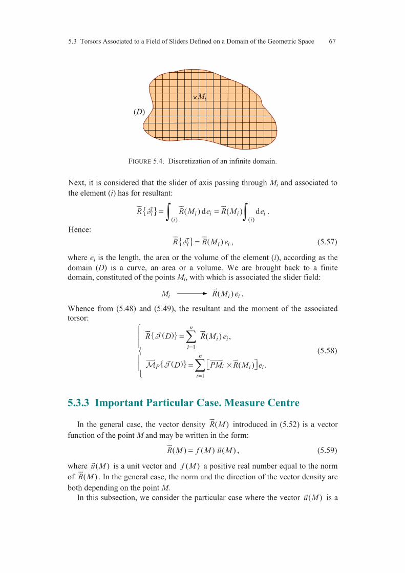
5.3 Torsors Associated to a Field of Sliders Defined on a Domain of the Geometric Space 67
FIGURE 5.4. Discretization of an infinite domain.
Next, it is considered that the slider of axis passing through Mi and associated to
the element (i) has for resultant:
( ) ( )
( ) d ( ) di i i i ii i
R R M e R M e= = .
Hence:
( )i i iR R M e= , (5.57)
where ei is the length, the area or the volume of the element (i), according as the
domain (D) is a curve, an area or a volume. We are brought back to a finite
domain, constituted of the points Mi, with which is associated the slider field:
Mi ( )i iR M e
.
Whence from (5.48) and (5.49), the resultant and the moment of the associated
torsor:
( )
( )
1
1
( ) ,
( ) .
n
i i
i
n
iP i i
i
R D R M e
D PM R M e
=
=
=
= ×
(5.58)
5.3.3 Important Particular Case. Measure Centre
In the general case, the vector density ( )R M
introduced in (5.52) is a vector
function of the point M and may be written in the form:
( ) ( ) ( )R M f M u M=
, (5.59)
where ( )u M
is a unit vector and ( )f M a positive real number equal to the norm
of ( )R M
. In the general case, the norm and the direction of the vector density are
both depending on the point M.
In this subsection, we consider the particular case where the vector ( )u M
is a
(D)
Mi

68 Chapter 5 Torsors
unit vector u
independent of the point M. The vector density is:
( ) ( ) R M f M u=
. (5.60)
The field of sliders defined on the domain (D) associates then at each point M a
slider of resultant:
( )M D∀ ∈ d ( ) ( ) d ( )R M f M u e M=
. (5.61)
The axes of the sliders defined on the domain (D) have thus all the same direction,
whatever the point M may be.
The elements of reduction, at an arbitrary point P of the geometric space, of the
torsor associated with such a field of sliders, are from (5.54) and (5.55):
( ) ( )
( ) d ( )D
R D u f M e M= , (5.62)
( ) ( )
( ) d ( )PD
D PM f M e M u
= ∧
. (5.63)
The moment vector ( ) P D is orthogonal to u
, hence to the resultant
( ) R D . The scalar invariant of the torsor ( ) D :
( ) ( ) ( ) PI D R D D= ⋅
(5.64)
is thus zero. It follows that the torsor ( ) D is either the null torsor, or a couple-
torsor, or a slider.
1. If ( )
( ) d ( ) 0D
f M e M = and ( )
( ) d ( ) 0D
PM f M e M u
× =
, the torsor
( ) D is the null torsor.
2. If ( )
( ) d ( ) 0D
f M e M = and ( )
( ) d ( ) 0D
PM f M e M u
× ≠
, the torsor
( ) D is a couple-torsor.
3. If ( )
( ) d ( ) 0D
f M e M ≠ , the torsor is a slider.
Hereafter in this subsection, we study the case where the torsor is a slider:
( )
( ) d ( ) 0D
f M e M ≠ . (5.65)
The resultant (5.62) of the slider can then be written in the form:
( ) ( ) R D D uµ= , (5.66)
on introducing the quantity:

5.3 Torsors Associated to a Field of Sliders Defined on a Domain of the Geometric Space 69
( )
( ) ( ) d ( )D
D f M e Mµ = . (5.67)
The quantity µ(D) thus defined is called the measure of the domain (D), associa-
ted to the field of sliders considered on (D). The quantity f(M) is the specific
measure (curvilinear, area or volume measure) at the point M.
Different fields of sliders can be associated to a same domain (D). Thus, it
follows that different measures will be associated to a same domain: volume (area
or length), mass, pressure, intensity of the gravitation field, intensity of the
electrostatic field, etc.
The torsor ( ) D considered being a slider, it has an axis of null moments
the points P of which, from (5.63), satisfy the relation:
( ) ( )
( ) d ( ) 0PD
D PM f M e M u
= × =
. (5.68)
Thus, the points of the axis are such as the vector ( )
( ) d ( )D
PM f M e M
is
collinear to u
. In particular, there exists a point of this axis, which we shall
denote by H such as the previous vector is zero. Whence:
( )
( ) d ( ) 0D
HM f M e M =
. (5.69)
The point H plays an important role and is called the measure centre related to the
field of the sliders considered on (D). We will say more briefly (but in an incur-
rect way) that H is the measure centre of the domain (D).
The position of the point H in the geometric space can be defined with respect
to a reference point O, by searching for the position vector OH
. Relation (5.69) is
written:
( )( )
( ) d ( ) 0D
OM HM f M e M− =
, (5.70)
or
( ) ( )
( ) d ( ) ( ) d ( )D D
OH f M e M OM f M e M=
. (5.71)
The position vector of the measure centre H is thus expressed in the form:
( )
1 ( ) d ( )( ) D
OH OM f M e MDµ
=
. (5.72)
Finally, the slider associated to the domain (D) and the field of sliders of
vector density ( ) ( ) R M f M u=
has a resultant given by Expression (5.66) and
an axis ( ), H u
of direction u
passing through the measure centre, defined by
(5.69) or (5.72).

70 Chapter 5 Torsors
In the case where the specific measure f(M) is independent of the point M:
( ) Constantf M k= = , (5.73)
Expression (5.72) is reduced to:
( )
1 d ( )( ) D
OH OM e Me D
=
, (5.74)
where e(D) is the length, the area or the volume of the domain (D). Relation
(5.74) shows that in this case the measure centre H is the same as the centroid of
the length, of the area or of the volume of the domain (D).
EXERCISES
5.1 Let (D) be the domain constituted of four points M1, M2, M3 and M4:
(D) = (M1, M2, M3 M4).
On this domain, we define a field of sliders, such as the resultants of the sliders
associated to each point are:
M1 (2, –2, 3) 1R
(5, 0, 0),
M2 (–4, 2, –1) 2R
(0, –2, 0),
M3 (5, –2, 3) 3R
(0, 0, 3),
M4 (0, 2, 0) 4R
(3, 4, 1).
The coordinates of the points are the Cartesian coordinates with respect to a refe-
rence system of origin O. The components of the resultants of the sliders are given
in the canonical basis.
Derive the resultant of the torsor associated to this field, its moment at the
point O. Characterize the torsor. Derive the moment of the torsor at an arbitrary
point P. Find the equations of the axis of the torsor.
5.2 We consider the same domain (D) as the one considered in the previous exer-
cise, but with a different field of sliders defined as follows:
M1 (2, –2, 3) 1R
(100, 0, 0),
M2 (–4, 2, –1) 2R
(0, 200, 50),
M3 (5, –2, 3) 3R
(–100, 0, –50),
M4 (0, 2, 0) 4R
(0, –200, 0).
Derive the resultant of the torsor associated to this field, its moment at O.
Characterize the torsor. Resolve the torsor at the origin point.

Exercises 71
5.3 Always to the domain (D), defined in Exercise 5.1, we associate the field of
sliders:
M1 (2, –2, 3) 1R
(5, – 4, 1),
M2 (–4, 2, –1) 2R
(0, –2, 0),
M3 (5, –2, 3) 3R
(0, 0, 3),
M4 (0, 2, 0) 4R
(3, 4, 1).
Derive the resultant of the torsor associated to this field, its moment at the
origin point O. Characterize the torsor. Derive the moment of the torsor at an
arbitrary point P. Find the equations of its central axis. Resolve the torsor at the
origin point.
5.4 Torsor associated to an infinite domain. We consider a domain (D) consti-
tuted of a rectangular surface ABCD (Figure 5.5). As reference system, we choose
the reference system (Axyz), of which the axes Ax
and Az
are respectively along
the sides AB and AD. To every area element dS(M) surrounding an arbitrary point
of the domain (D), we associate the slider of vector density ( ) p M i
. The field of
sliders thus defined on the domain (D) associates to every point M a slider of
resultant:
d ( ) ( ) d ( )R M p M i S M=
,
and axis ( ), M i
.
Derive the torsor associated to this field of sliders.
FIGURE 5.5. Rectangular domain.
(D)
A B
C D
M
dS(M)
x
z
y
72 Chapter 5 Torsors
COMMENTS
The formalism of torsor constitutes the key of the concepts which will
be introduced in the continuation of this textbook. Thus, the reader will
have to study thoroughly all the elements considered in the present chapter.
The concept of vector makes it possible to work simultaneously on three
real numbers. The concept of torsor makes it possible to operate simulta-
neously on two vectors, the resultant of the torsor and its moment.
Three types of torsors exist: slider, couple-torsor and arbitrary torsor.
The type of torsor is characterized by its scalar invariant. The slider consti-
tutes the fundamental type of torsor, since a couple-torsor can be resolved
into the sum of a couple of two sliders, and an arbitrary torsor can be
resolved into a slider and a couple-torsor.
The reader will pay a particular attention to Subsection 5.3.3 which
considers the very important case for which there is a measure centre.
The exercises suggested illustrate simply the whole of the concepts
which are introduced into the chapter.

Part II
Kinematics
Kinematics is part of Mechanics whose the object is the study of
the motion of a physical system: point or particle, rigid body, set of
rigid bodies, etc., without reference to the cause of the motion. Kine-
matics is used to relate displacement, velocity, acceleration, and time.
Causes of the motions will be considered as part of Dynamics (Part
IV).
Kinematics of point (or particle) consists in characterizing the
motion of a point with respect to a reference system: first, the place
(the trajectory) where the point is moving; then, how it is moving on
this trajectory (quickly, slowly, more and more quickly, less and less
quickly, etc.). The way of moving on the trajectory will be charac-
terized by the kinematic vectors of the point: velocity vector and acce-
leration vector.
The object of the Kinematics of rigid body is to establish the rela-
tions between the motions of all the points of a given rigid body. The
relation between the trajectories of the points is brought back to the
problem of the change of coordinates, problem which was considered
previously in Chapter 2. The relations between the velocity vectors
will be characterized by introducing the notion of kinematic torsor.
Kinematics of two solids in contact needs a particular analysis
which introduces the notion of sliding, rolling and spinning.

CHAPTER 6
Kinematics of Point
6.1 INTRODUCTION
To translate into equations the motions of physical systems, an observer has to
schematize the space which surrounds him. The assumed schematization is that of
the geometric space (Chapter 2). In particular, the observer will be brought to
choose a reference system (apparatus frame, part of the Earth surface, moving
train, etc.), to which the observer will link reference axes and with respect to
which the observer will analyse the motions.
With the schematization of the space, the observer must add the notion of time.
This notion makes it possible to give an account of the simultaneity of two events,
of the order of succession of these two events and the duration of the interval
which separates them. The measurement of a duration is related to the choice of a
measurement unit (the international unit is the second: s). This measurement is
implemented using clocks (watch, Earth motion, etc.) associated with a calendar
With the indications provided by a clock and a calendar, we associate the
numerical value of a variable called time variable, and which we will denote by t.
We call date of an instantaneous event then, the numerical value t at the moment
when the event occurs. If t1 is the date of an event E1, and t2 that of an event E2,
the duration of the interval which separates them is 2 1t t− . By convention, it has
been chosen to take 2 1 0,t t− > when E2 is posterior to E1. It is said that the time
scale is increasing in the succession of the events.
6.2 TRAJECTORY AND
KINEMATIC VECTORS OF A POINT
Let (T) be a reference system that we will simply call reference, and let (D) be
a set (Figure 6.1) of which we want to study the motion with respect to reference
(T). The reference system (T) is such as each one of its points is motionless with

76 Chapter 6 Kinematics of Point
FIGURE 6.1. Motion of a set (D) with respect to a reference (T).
respect to the other points. It is the same for the set (D). We will call M an arbi-
trary point of the set (D) and O a point of the reference system (T), chosen as refe-
rence point
6.2.1 Trajectory
The position of point M with respect to the reference (T) is defined by the
vector OM
. If the set (D) is moving with respect to (T), the vector OM
is a
vector function of the time:
( )OM V t=
. (6.1)
When t varies, the point M follows a curve (Chapter 4) defined by the preceding
relation and called the trajectory of the point M with respect to the reference (T).
The trajectory is the set of the points of the reference (T) with which the point M
comes in coincidence at every moment (Figure 6.2).
FIGURE 6.2. Trajectory in a given reference.
M
(D)
(T)
O
trihedron attached
to reference (T)
reference system
(reference)
O
M
reference (T )
trajectory in the
reference (T )
points of
reference (T )

6.2 Trajectory and Kinematic Vectors of a Point 77
The trajectory depends on the reference system. For example, if we consider a
traveller sitting in a train moving with a rectilinear motion, the trajectory of this
traveller with respect to a reference linked to the Earth is a line segment, whereas
the trajectory with respect to the coach is reduced to a point.
6.2.2 Kinematic Vectors
The trajectory is not sufficient to characterize the motion of a point completely.
In addition to the geometrical nature, it is necessary to specify the motion of the
point on this trajectory. The study of this motion is conducted by studying the
vector function ( )V t
(Relation 6.1), which leads to introduce the first and second
derivatives with respect of the time of the position vector OM
. These two vectors
are called the kinematic vectors of the point M and make it possible to entirely
characterize the motion of the point on its trajectory.
6.2.2.1 Velocity Vector
The first kinematic vector is the velocity vector, vector derivative, with respect
to the time and relatively to the reference (T), of the position vector of the point
M, hence:
( )( )( )
d,d
TT M t OM
t=
. (6.2)
The notation ( )( ),T M t expresses the fact that we consider the velocity vector,
relatively to the reference (T), of the point M, at the date t. This notation will be
simplified when there will be no possible confusion: ( ) ( )( ) ( ) , , ,TM t M M or
. The notation
( )dd
T
t expresses the fact that the derivation with respect to the
time is carried out in a basis related to the reference (T).
The velocity is a continuous function of the time function, except at the times of
collisions between bodies. Such events must then be the subject of particular
studies.
6.2.2.2 Acceleration Vector
The second kinematic vector is the acceleration vector, second derivative
vector, with respect to the time and relatively to the reference (T), of the position
vector of the point M:
( )( )( ) ( )
( )( )
2
2
d d, ,dd
T TTM t OM M t
tt= =
. (6.3)
As in the case of the velocity vector, the notation of the acceleration vector could
be simplified.
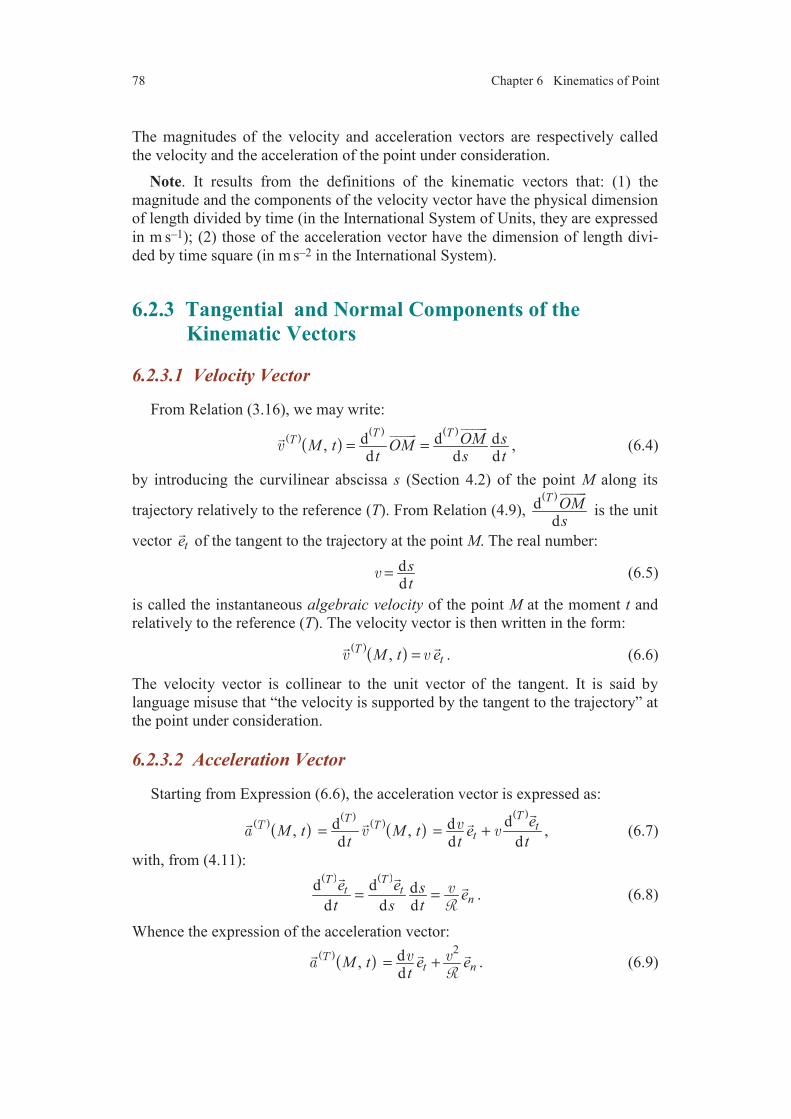
78 Chapter 6 Kinematics of Point
The magnitudes of the velocity and acceleration vectors are respectively called
the velocity and the acceleration of the point under consideration.
Note. It results from the definitions of the kinematic vectors that: (1) the
magnitude and the components of the velocity vector have the physical dimension
of length divided by time (in the International System of Units, they are expressed
in m s–1); (2) those of the acceleration vector have the dimension of length divi-
ded by time square (in m s–2 in the International System).
6.2.3 Tangential and Normal Components of the Kinematic Vectors
6.2.3.1 Velocity Vector
From Relation (3.16), we may write:
( )( )( ) ( )
d d d,d d d
T TT OM sM t OM
t s t= =
, (6.4)
by introducing the curvilinear abscissa s (Section 4.2) of the point M along its
trajectory relatively to the reference (T). From Relation (4.9), ( )
dd
T OMs
is the unit
vector te
of the tangent to the trajectory at the point M. The real number:
dd
st
= (6.5)
is called the instantaneous algebraic velocity of the point M at the moment t and
relatively to the reference (T). The velocity vector is then written in the form:
( )( ),TtM t e=
. (6.6)
The velocity vector is collinear to the unit vector of the tangent. It is said by
language misuse that “the velocity is supported by the tangent to the trajectory” at
the point under consideration.
6.2.3.2 Acceleration Vector
Starting from Expression (6.6), the acceleration vector is expressed as:
( )( )( )
( )( )( )
dd d, ,d d d
TTT t
te
M t M t et t t
= = +
, (6.7)
with, from (4.11): ( ) ( )
d d dd d d
T Tt t
ne e s e
t s t= =
. (6.8)
Whence the expression of the acceleration vector:
( )( )2d,
dt nM t e e
t= +
. (6.9)

6.2 Trajectory and Kinematic Vectors of a Point 79
We call tangential acceleration vector, the vector:
dd
t ta et
= , (6.10)
and normal acceleration vector, the vector: 2
n na e=
. (6.11)
Relation (6.9) is then written: ( )( ), t nM t a a= +
, (6.12)
or ( )( ) , t t n nM t a e a e= +
, (6.13)
where at and an are the tangential and normal components of the acceleration
vector: 2d ,
dt na a
t= =
. (6.14)
The normal component is always positive. The tangential component is positive if
the algebraic velocity is increasing, and negative on the contrary.
6.2.3.3 Representation of the Kinematic Vectors
The velocity vector and the acceleration vector are vectors of the space 3. It
happens however that, by convention, one represents, in the geometric space, the
bipoints having for origin the position of the point M at the date t and having for
images the kinematic vectors of the point M (Figure 6.3).
6.2.4 Different Types of Motions
6.2.4.1 Definitions
We shall say that the motion of the point M is:
— accelerated at time t, if the magnitude of the velocity vector ( )( ),T M t is
increasing at this moment;
FIGURE 6.3. Symbolic representation of the kinematic vectors.
te M(t)
(C)
ne
( )( ),T M t
dd
tat
=
( )( ),M t2
na =
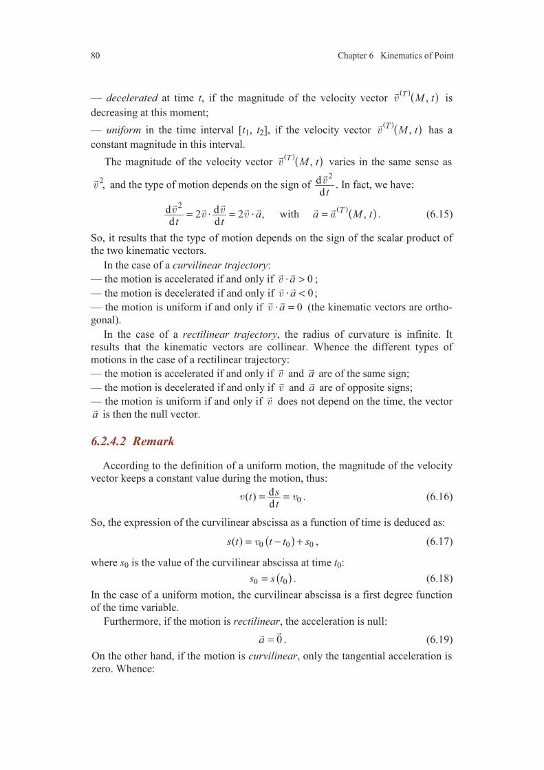
80 Chapter 6 Kinematics of Point
— decelerated at time t, if the magnitude of the velocity vector ( )( ),T M t is
decreasing at this moment;
— uniform in the time interval [t1, t2], if the velocity vector ( )( ),T M t has a
constant magnitude in this interval.
The magnitude of the velocity vector ( )( ),T M t varies in the same sense as
2, and the type of motion depends on the sign of
2dd t
. In fact, we have:
( )( )
2d d2 2 , with ,d d
a a M tt t
= = =⋅ ⋅
. (6.15)
So, it results that the type of motion depends on the sign of the scalar product of
the two kinematic vectors.
In the case of a curvilinear trajectory:
— the motion is accelerated if and only if 0a >⋅ ;
— the motion is decelerated if and only if 0a <⋅ ;
— the motion is uniform if and only if 0a =⋅ (the kinematic vectors are ortho-
gonal).
In the case of a rectilinear trajectory, the radius of curvature is infinite. It
results that the kinematic vectors are collinear. Whence the different types of
motions in the case of a rectilinear trajectory:
— the motion is accelerated if and only if and a
are of the same sign;
— the motion is decelerated if and only if and a
are of opposite signs;
— the motion is uniform if and only if does not depend on the time, the vector
a
is then the null vector.
6.2.4.2 Remark
According to the definition of a uniform motion, the magnitude of the velocity
vector keeps a constant value during the motion, thus:
0d( )d
stt
= = . (6.16)
So, the expression of the curvilinear abscissa as a function of time is deduced as:
( )0 0 0( )s t t t s= − + , (6.17)
where s0 is the value of the curvilinear abscissa at time t0:
( )0 0s s t= . (6.18)
In the case of a uniform motion, the curvilinear abscissa is a first degree function
of the time variable.
Furthermore, if the motion is rectilinear, the acceleration is null:
0a =
. (6.19)
On the other hand, if the motion is curvilinear, only the tangential acceleration is
zero. Whence:

6.3 Expressions of the Components of the Kinematic Vectors 81
20
n na a e= =
. (6.20)
These results call the following remark. When one speaks about “velocity”, it is
necessary to specify if it is the velocity, the algebraic velocity, or the magnitude
of the velocity vector, which is concerned. Thus, we have just seen that a motion
with a constant magnitude of the velocity vector is, either rectilinear, or curvi-
linear. On the other hand, a motion with constant velocity vector is necessarily
rectilinear. This remark also applies to the “acceleration”.
6.3 EXPRESSIONS OF THE COMPONENTS OF THE
KINEMATIC VECTORS AS FUNCTIONS OF THE
CARTESIAN AND CYLINDRICAL COORDINATES
6.3.1 Cartesian Coordinates
We consider the case where the point M in the reference (T) is characterized by
the Cartesian coordinates (x, y, z) relatively to the coordinate system (Oxyz) fixed
with respect to the reference (T) (Figure 2.12). The position vector is written:
OM x i y j z k= + +
, (6.21)
where ( ) , ,i j k
is the canonical basis of the vector space 3.
According to the relations of definitions (6.2) and (6.3) of the kinematic
vectors, and the concepts introduced in Chapter 3, the expressions of the kine-
matic vectors are written as:
( )( )( )
dd d d,d d d d
TT yx zM t OM i j k
t t t t= = + +
, (6.22)
( )( )( )
( )( )
22 2
2 2 2
dd d d, ,d d d d
TT yx zM t M t i j k
t t t t= = + +
. (6.23)
It is usual to introduce in the expressions for the derivatives as functions of
time the condensed notations:
— ( )f t or f for the first derivative with respect to time of the function f(t);
— ( )f t or f for the second derivative.
With such notations, Expressions (6.22) and (6.23) are written:
( )( ) ,T M t x i y j z k= + +
, (6.24)
( )( ) ,M t x i y j z k= + +
. (6.25)

82 Chapter 6 Kinematics of Point
6.3.2 Cylindrical Coordinates
The cylindrical coordinates (r, α, z) of a point M with respect to the coordinate
system Oxyz have been introduced in Subsection 3.3.2.1 (Figure 3.1). It has been
shown that:
( )OM r u z kα= +
, (6.26)
( )d ( ) ( )d 2
T
u u πα αα
= +
,
( )d ( ) ( ) ( )d 2
T
u u uπα α π αα
+ = + = −
(6.27)
( )d d d d( ) ( )d d d 2 d
T OM r zu r u kt t t t
α πα α= + + +
, (6.28)
where ( )u α
is the unit vector of the projection of the bipoint (O, M) in the plane
Oxy, and ( )2
u πα +
is the unit vector of the direction of the plane Oxy orthogonal
to the preceding direction (Figure 3.1).
The cylindrical coordinates make it possible to express the kinematic vectors
in the basis ( ), ( ), 2
u u kπα α +
. Thus, from (6.28) we have:
( )( , ) ( ) ( )
2T M t r u r u z kπα α α= + + +
. (6.29)
The components of the velocity vector in the basis ( ), ( ), 2
u u kπα α +
are:
( ), , r r zα . (6.30)
To obtain the expression of the acceleration vector, it is necessary to derive
with respect to time Expression (6.29) of the velocity vector taking account of the
relations:
( ) ( )d d d( ) ( ) ( )d d d 2
T T
u u utα πα α α α
α α= = +
, (6.31)
( ) ( )d d d( ) ( ) ( )d 2 d 2 d
T T
u u ut t
π π αα α α αα
+ = + = −
. (6.32)
We obtain then:
( )( ) ( ) ( ) 2, ( ) 2 ( )
2M t r r u r r u z kπα α α α α= − + + + +
. (6.33)
The components of the acceleration vector in the basis ( ), ( ), 2
u u kπα α +
are:
( )2 , 2 , r r r r zα α α− + . (6.34)
In the case where the trajectory of point M is plane, it is possible to choose the
coordinate system (Oxyz) so that the plane (Oxy) contains the trajectory. The
cylindrical coordinates of point M are then (r, α, 0), and the parameters (r, α) are
called the polar coordinates of point M. The expressions of the kinematic vectors
Exercises 83
are deduced from Relations (6.29) and (6.33), with 0z z= = . We obtain:
( )( , ) ( ) ( )
2T M t r u r u πα α α= + +
, (6.35)
( )( ) ( ) ( )2, ( ) 2 ( )2
M t r r u r r u πα α α α α= − + + +
. (6.36)
EXERCISES
6.1 The motion of a point M is defined by its Cartesian coordinates as functions
of time:
( )2 2 3 33 , 3 , 0,x a t y a t t zω ω ω= = − =
where a and ω are positive constants (a is a length and ω is the inverse of time).
1. Plot the trajectory of the point M for 0t ≥ .
2. Derive as functions of time t: the velocity vector; the instantaneous algebraic
velocity; the acceleration vector and its tangential and normal components; the ra-
dius of curvature of the trajectory.
6.2 Two cities A and B are distant of 160 km. A cyclist leaves A at 8 h, and
moves toward B at the average speed of 30 km/h. At 9 h a car leaves A in
direction of B, with an average speed of 85 km/h. Lastly, a truck starts at 9h30
from B towards A, with an average speed of 60 km/h.
1. Establish the motion equations for the cyclist, the car, the truck.
2. Derive the places and the dates at which:
— the car draws ahead of the cyclist;
— the truck meets the car, the cyclist.
COMMENTS
The motion of a point of a rigid body is defined by the place where it
moves: the trajectory, and by the way in which it moves on this trajectory:
quickly, slowly, more and more quickly, more and more slowly. The way
in which the point moves on its trajectory is characterized by its kinematic
vectors of the point: velocity vector and acceleration vector. Trajectory and
kinematic vectors depend of the reference system in which the motion is
observed. The expressions of the kinematic vectors are obtained simply as
functions of the Cartesian coordinates. The reader will give a particular
attention to the determination of the kinematic vectors as functions of the
cylindrical coordinates.

O
(D)
M
x
M
(D)
y
z
CHAPTER 7
Study of Particular Motions
7.1 MOTIONS WITH RECTILINEAR TRAJECTORY
7.1.1 General Considerations
The trajectory of a point M in the reference (T) is rectilinear, if the point M
moves along a straight line belonging to (T) (Figure 7.1). We may choose a
coordinate system (Oxyz) fixed to the reference (T), such as the axis Ox
coincides
with the line (D). The position vector is then written as:
.OM x i=
(7.1)
The velocity vector of the point M is:
,x i= (7.2)
and its acceleration vector is:
.a x i= (7.3)
FIGURE 7.1 Rectilinear trajectory.
7.1 Motions with Rectilinear Trajectory 85
7.1.2 Uniform Rectilinear Motion
The motion of a point M is rectilinear uniform, if and only if the velocity vector
is constant:
0 0cst i= = =
(7.4)
where 0 is independent of time. The acceleration vector is null.
From (7.2), we have:
0dd
x xt
= = . (7.5)
Hence while integrating:
0 cstx t= + . (7.6)
If at the time t = t0, the point M is at M0, such as 0 0 ,OM x i=
we obtain:
( )0 0 0x t t x= − + . (7.7)
In the particular case where the point M is at the origin O at the time origin 0,t =
Equation (7.7) is reduced to:
0x t= . (7.8)
7.1.3 Uniformly Varied Rectilinear Motion
The motion of a point M is rectilinear uniformly varied, if and only if the acce-
leration vector is constant:
0a a i=
(7.9)
where a0 is independent of time.
We have: 2
02
d
d
x x at
= = . (7.10)
By integrating twice, we obtain:
( )0 0 0a t t= − + , (7.11)
( ) ( )200 0 0 0
2
ax t t t t x= − + − + , (7.12)
the point M being at the time t0 at M0, such as 0 0 ,OM x i=
with a velocity 0 .i
In the particular case where the point M is at the origin O with a zero velocity
at the time origin 0,t = the motion equations (7.11) and (7.12) are reduced as:
0a t= , 20
2
ax t= . (7.13)
Between the variables x and , there exists the general relation obtained by eliminating the time in (7.11) and (7.12):
( ) ( )2 20 0 0
12
a x x− = − . (7.14)
86 Chapter 7 Study of Particular Motions
From the results derived in Subsection 6.2.4.1, we deduce that the motion is:
— uniformly accelerated, if 0 0a > ;
— uniformly decelerated or retarded, if 0 0a < .
7.1.4 Simple Harmonic Rectilinear Motion
The rectilinear motion of a point M is a simple harmonic motion, if the motion
is described by the law:
cos sinx A t B tω ω= + , (7.15)
or
( )cosmx x tω ϕ= − . (7.16)
Between the constants A, B, xm and ϕ, we have the relations:
2 2 1
cos , sin ,
, tan , with cos .
m m
mm
A x B x
B Ax A BA x
ϕ ϕ
ϕ ϕ−
= =
= + = = (7.17)
Without restricting the generality of the study, the constant ω is taken positive.
The algebraic velocity is:
sin cosx A t B tω ω ω ω= − + ,
or (7.18)
( )sinmx x tω ω ϕ= − − .
The acceleration vector has for component:
2 2cos sinx A t B tω ω ω ω= − − ,
or (7.19)
( )2 cosmx x tω ω ϕ= − − .
From these expressions, we draw the relation:
2 2 ou x x a OMω ω= − = −
, (7.20)
and the expressions of the constants:
00
22 10 0 0
0 20
, ,
, tan , with cos ,mm
A x B
xx x
x x
ω
ϕ ϕωω
−
= =
= + = =
(7.21)
where x0 and 0 are the respective values of the variables x and at time t = 0.
The variations of x are reported in Table 7.1. The point M oscillates indefini-
tely between the extreme points xm and –xm, with the period 2T π ω= . The quan-
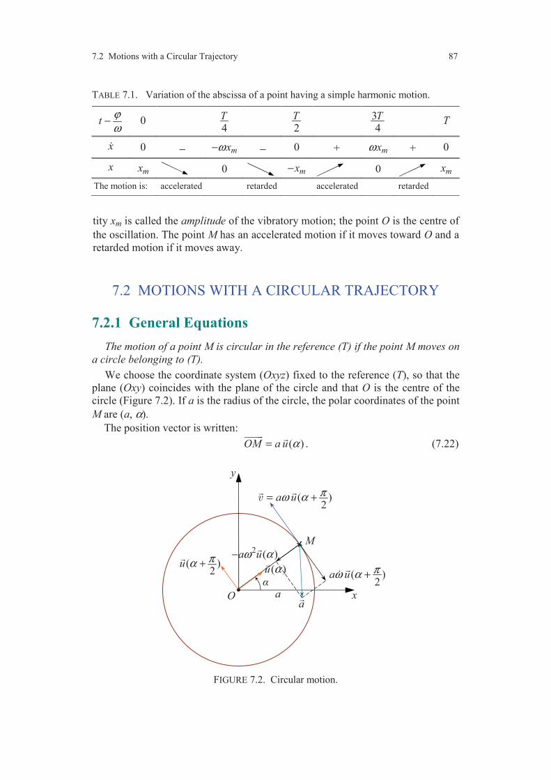
7.2 Motions with a Circular Trajectory 87
TABLE 7.1. Variation of the abscissa of a point having a simple harmonic motion.
tϕω
− 0 4T
2T 3
4T T
x 0 − mxω− − 0 + mxω + 0
x mx 0 mx− 0 mx
The motion is: accelerated retarded accelerated retarded
tity xm is called the amplitude of the vibratory motion; the point O is the centre of
the oscillation. The point M has an accelerated motion if it moves toward O and a
retarded motion if it moves away.
7.2 MOTIONS WITH A CIRCULAR TRAJECTORY
7.2.1 General Equations
The motion of a point M is circular in the reference (T) if the point M moves on
a circle belonging to (T).
We choose the coordinate system (Oxyz) fixed to the reference (T), so that the
plane (Oxy) coincides with the plane of the circle and that O is the centre of the
circle (Figure 7.2). If a is the radius of the circle, the polar coordinates of the point
M are (a, α).
The position vector is written:
( )OM a u α=
. (7.22)
FIGURE 7.2. Circular motion.
x
M
y
a
( )2
a u πω α= +
( )2
a u πω α +
2 ( )a uω α−
( )u α( )
2u πα +
aO

88 Chapter 7 Study of Particular Motions
Differentiating this expression, we obtain successively the velocity and acce-
leration:
( )( , ) ( )
2T M t a u πα α= +
, (7.23)
( ) 2( , ) ( ) ( )2
Ta M t a u a u πα α α α= − + +
. (7.24)
The parameter α is called the angular velocity (measured in rad s–1) of the point
M, at the time t. It is generally denoted by ω:
ddtαω α= = . (7.25)
The parameter α is the angular acceleration (measured in rad s–2) of the point M:
ddtωα ω= = . (7.26)
The expressions of the kinematic vectors can then rewritten while introducing
the angular velocity as:
( )( , ) ( ),
2T
M t a u πω α= + (7.27)
( ) 2( , ) ( ) ( ).2
Ta M t a u a u πω α ω α= − + +
(7.28)
The algebraic velocity of the point M at the time t is:
aω= . (7.29)
The acceleration vector has:
— a tangential component:
ta aω= , (7.30)
— a normal component:
2na aω= − . (7.31)
The acceleration vector na
is always of opposite sign to the position vector OM
:
2na OMω= −
. (7.32)
Lastly, the motion is: accelerated, if 0 ;ωω > retarded, if 0 ;ωω < uniform, if
0.ω =
7.2.2 Uniform Circular Motion
A circular motion is uniform, if its angular frequency is independent of time.
Whence:
0cstω ω= = . (7.33)
The kinematic vectors (7.27) and (7.28) are reduced to:
7.2 Motions with a Circular Trajectory 89
( ) 0( , ) ( )
2T
M t a u πω α= + , (7.34)
( ) 20( , ) ( )Ta M t a uω α= −
. (7.35)
The tangential component of the acceleration vector is zero. Whence it results that
the acceleration vector is collinear to the position vector:
( ) 20( , )Ta M t OMω= −
. (7.36)
In addition, the motion law is written as:
( )0 0 0t tα ω α= − + ,
where α0 is the value of the angle α at the time t0.
Lastly, in a uniform circular motion, the actual parameter is the number of
revolution N per unit of time. The angular velocity is then expressed by the
relation:
0 2 Nω π= . (7.37)
7.2.3 Uniformly Varied Circular Motion
A circular motion is uniformly varied, if its angular acceleration is indepen-
dent of time. Thus:
0d cstdtωα ω= = = . (7.38)
Expressions (7.27) and (7.28) of the kinematic vectors are written:
( )( , ) ( )
2T
M t a u πω α= + , (7.39)
( ) 20( , ) ( ) ( )
2Ta M t a u a u πω α ω α= − + +
. (7.40)
The tangential component of the acceleration vector is constant.
The motion law is written as:
( )
( ) ( )
0 0 0
200 0 0 0
,
,2
t t
t t t t
α ω ω ω
ωα ω α
= = − +
= − + − +
(7.41)
where ω0 and α0 are the respective values of ω and α at the time t0.
Lastly, the motion is uniformly:
— accelerated, if 0 0 ;ωω >
— retarded, if 0 0 .ωω <

90 Chapter 7 Study of Particular Motions
7.3 MOTIONS WITH A CONSTANT
ACCELERATION VECTOR
7.3.1 General Equations
The motion of a point M with a constant acceleration vector is such as:
( )0( , )Ta M t a=
(7.42)
where the vector 0a
is a vector independent of time.
We choose (Figure 7.3), as coordinate reference, the system (Oxyz) so that the
vector 0a
is the direction vector of the axis Oz
( 0a
is collinear to k
). In addition,
to adapt the investigation to the analysis of the motion of projectiles in the vicinity
of the Earth surface, we take the determination:
0 0a a k= −
(7.43)
with 0 0a > .
By integrating the expression:
( )( )
( ) 0
d( , ) ( , )d
TT Ta M t M t a k
t= = −
, (7.44)
we obtain: ( )
0 0( , )T M t a t k= − +
, (7.45)
introducing the velocity vector 0 at the time 0t = :
( )0 ( , 0)T M t= = . (7.46)
We characterize the direction given by the vector 0 , by introducing (Figure
7.3) the angle 2π ϕ+ between the axis ( )0,O
and the axis ( )0,O a
. The axis Oy
is then chosen so that the plane (Oyz) contains the axis ( )0,O and so that this
axis forms an angle ϕ with the axis Oy
. The coordinate system is then entirely
FIGURE 7.3. Motion with a constant acceleration vector.
0
0ax
y
z
O
k

7.3 Motions with a Constant Acceleration Vector 91
defined. This particular choice of the coordinate system is well adapted to the
analysis of the motions of projectiles in the vicinity of the Earth surface. By intro-
ducing the magnitude 0 of the velocity vector 0 at the time 0t = , we can write:
( )0 0 cos sinj kϕ ϕ= +
. (7.47)
Thus, by substituting into Expression (7.45):
( )( )
( )0 0 0d( , ) cos sin
d
TT OMM t j k a t
tϕ ϕ= = + −
. (7.48)
By integrating twice with respect to time, we obtain:
( )200 0 0cos sin
2
aOM OM j t k t tϕ ϕ= + + −
, (7.49)
the point M being at point M0 at the time 0.t =
If we choose a coordinate system, such as the point M is at the origin O at the
time 0,t = the motion equation is reduced to:
( )200 0cos sin
2
aOM j t k t tϕ ϕ= + −
. (7.50)
The Cartesian coordinates of the point M relatively to the system (Oxyz) are then:
200 00, cos , sin .
2
ax y t z t tϕ ϕ= = = − (7.51)
The trajectory is contained into the plane (Oyz). If 2πϕ = ± , the trajectory is recti-
linear and supported by the axis Oz. If 2πϕ ≠ ± , the trajectory is a parabola.
7.3.2 Study of the case where the Trajectory is Rectilinear
7.3.2.1 Case where2πϕ =
From (7.51), the point M has for coordinates:
2000, 0, .
2
ax y z t t= = = − (7.52)
The velocity vector ( )
( , )T M t has for components:
0 00, 0, .x y z a t= = = − (7.53)
We deduce from these results the table 7.2 of the variations. The point M
moves away from O along the half-axis Oz
of positive abscissae, with a retarded
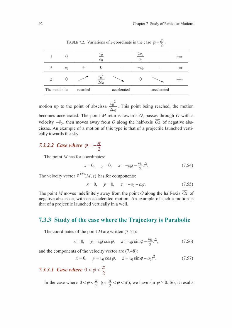
92 Chapter 7 Study of Particular Motions
TABLE 7.2. Variations of z-coordinate in the case 2πϕ = .
t 0 0
0a
0
0
2
a
+∞
z 0 + 0 − 0− − −∞
z 0 2
0
02a
0 −∞
The motion is: retarded accelerated accelerated
motion up to the point of abscissa 2
0
02a
. This point being reached, the motion
becomes accelerated. The point M returns towards O, passes through O with a
velocity 0− , then moves away from O along the half-axis Oz
of negative abs-
cissae. An example of a motion of this type is that of a projectile launched verti-
cally towards the sky.
7.3.2.2 Case where 2πϕ = −
The point M has for coordinates:
2000, 0, .
2
ax y z t t= = = − − (7.54)
The velocity vector ( )
( , )T M t has for components:
0 00, 0, .x y z a t= = = − − (7.55)
The point M moves indefinitely away from the point O along the half-axis Oz
of
negative abscissae, with an accelerated motion. An example of such a motion is
that of a projectile launched vertically in a well.
7.3.3 Study of the case where the Trajectory is Parabolic
The coordinates of the point M are written (7.51):
200 00, cos , sin ,
2
ax y t z t tϕ ϕ= = = − (7.56)
and the components of the velocity vector are (7.48): 2
0 0 00, cos , sin .x y z a tϕ ϕ= = = − (7.57)
7.3.3.1 Case where 02πϕ< <
In the case where 02πϕ< < (or
2π ϕ π< < ), we have sin ϕ > 0. So, it results

7.3 Motions with a Constant Acceleration Vector 93
TABLE 7.3. Variations of z-coordinate in the case where 0 .2πϕ< <
t 0 0
0
sina
ϕ 0
0
2 sina
ϕ
+∞
z 0 sinϕ + 0 − 0 sinϕ− − −∞
z 0 2
20
0
sin2a
ϕ
0 −∞
y 0 2
0
0
sin 22a
ϕ
20
0
sin 2a
ϕ
+∞
the motion is: retarded accelerated accelerated
from (7.56) that at the beginning of the motion z is positive, then passes by a
maximum, is zero for 0
0
2 sinta
ϕ=
and becomes negative. The variations are
reported in Table 7.3. The trajectory is drawed in Figure 7.4. The motion of the
point M is retarded on the arc of parabola OH , H being the summit of the para-
bola of coordinates: 2 2
20 0
0 0
0, sin 2 , sin2 2
H H Hx y za a
ϕ ϕ= = =
. (7.58)
The motion is then accelerated, the point M passing through the point P (called
the horizontal range) of the axis Oy
:
20
0
0, sin 2 , 0P P Px y za
ϕ= = =
, (7.59)
FIGURE 7.4. Parabolic trajectory in the case 0 .2πϕ< <
0
0 0a a k= −
y
z
O
k
H
P 20
0
sin 22a
ϕ
20
0
sin 2a
ϕ
220
0
sin2a
ϕ
retarded
accelerated

94 Chapter 7 Study of Particular Motions
with a velocity of components:
0 00, cos , sinP P Px y zϕ ϕ= = = − . (7.60)
In a general way, we observe that the magnitude of the velocity is the same one
at two points of the same z-coordinates (the components along k
being opposite).
Moreover, the distance from O to P is maximum and equal to 2
0
0a
, if
4πϕ = .
An example of such a motion is that of a projectile launched in the direction
which forms an angle ϕ with the Earth surface (the plane (Oxy) is then the hori-
zontal plane). The angle ϕ is the fire angle, the z-coordinate zH is the maximum
altitude reached by the projectile, and the distance from O to P is the horizontal
range of firing.
7.3.3.2 Case where 02π ϕ− < <
In the case where 02π ϕ− < < (or 3
2ππ ϕ< < ), we have sin 0ϕ < . It results
from (7.56) that z is always negative. As in the preceding case, the trajectory is an
arc of parabola tangent at the point O to the line ( )0, O , and contained in the
plane ( 0, 0y z≥ ≤ ) (Figure 7.5). The motion of the point M is constantly accele-
rated.
An example of such a motion is given by the motion of a projectile launched
with a negative fire angle, for example from a tower or a plane.
7.4 HELICOIDAL MOTION
A point M moves with a helicoidal motion in a given reference, if its trajectory
is a right circular helix, drawn on a right cylinder (Figure 7.6).
FIGURE7.5. Parabolic trajectory in the case 02π ϕ− < < .
0
0 0a a k= −
y
z
O
accelerated

7.4 Helicoidal Motion 95
In the coordinate system (Oxyz), the parametric representation of the helix can
be written, for the Cartesian coordinates of the point M, in the form:
cos , sin , ,x a y a z bα α α= = = (7.61)
where α is the angle of the cylindrical coordinates (an arbitrary function of time).
The quantity a is the radius of the cylinder on which the helix is drawn. The
parameter b is the reduced pitch of the helix: increasing the angle α by 2π leads
to translate the helix of 2 bkπ
since:
( 2 ) ( ),
( 2 ) ( ),
( 2 ) ( ) 2 .
x x
y y
z z b
α π α
α π α
α π α π
+ =
+ =
+ = +
(7.62)
The position vector is written:
( )OM a u b kα α= +
. (7.63)
Thence we deduce the kinematic vectors:
( ) ( , ) ( )
2M t a u b kπα α α= + +
, (7.64)
( )
2( , ) ( ) ( )2
Ta M t a u a u b kπα α α α α= − + + +
. (7.65)
The ratio of the components of the velocity vector is:
b ba aαα
=
(7.66)
which is independent of α. So, it results that the tangent at any point M of the helix
forms a constant angle with the axis ( ),M k
, parallel to the axis of the cylinder.
FIGURE 7.6. Helicoidal motion.
y
z
M
D
O a
x
k
( )u α
( )2
u πα +
( )2
a u πα α +
b kα
( )( , )T M t
helix
96 Chapter 7 Study of Particular Motions
The helicoidal motion is uniform if:
0α ω= (7.67)
where ω0, the angular velocity of rotation, is independent of time. The kinematic
vectors are written in this case:
( ) 0 0( , ) ( )
2M t a u b kπω α ω= + +
, (7.68)
( )
20( , ) ( )Ta M t a uω α= −
. (7.69)
The algebraic velocity is deduced from (7.68) as:
2 20a b ω= + . (7.70)
For a uniform motion, the acceleration vector has only a normal component (6.9).
Hence it results that the principal normal at the point M of the helix is the normal
to the cylinder at this point :
( )ne u α= −
. (7.71)
Relations (7.68) and (7.69) compared to the expression (6.9) make it possible to
derive the radius of curvature of the helix. Thus:
2baa
= + . (7.72)
The curvature centre D (4.17) is defined by the relation:
( )MD u α= −
. (7.73)
7.5 CYCLOIDAL MOTION
A point M moves with a cycloidal in a given reference, if its trajectory is a
cycloid. The Cartesian coordinates of the point M relatively to a coordinate
system linked to this reference are written as:
( ) ( )sin , 1 cos , 0,x a q q y a q z= − = − = (7.74)
where q is a parameter which is a function of time.
An example of cycloidal motion is given by the motion of a point M of a disk
or wheel of radius a, rolling on the axis Ox
(Figure 7.7). By taking account of the
equality OH HM= , we obtain really Expressions (7.74) of the coordinates of the
point M.
If we increase the angle q by 2π, Expressions (7.74) show that:
( 2 ) ( ) 2 ,
( 2 ) ( ),
0.
x q x q a
y q y q
z
π π
π
+ = +
+ =
=
(7.75)
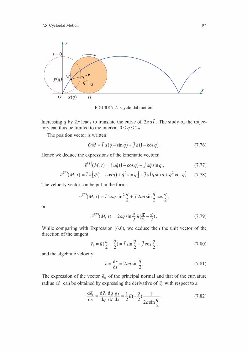
7.5 Cycloidal Motion 97
FIGURE 7.7. Cycloidal motion.
Increasing q by 2π leads to translate the curve of 2 a iπ
. The study of the trajec-
tory can thus be limited to the interval 0 2q π≤ ≤ .
The position vector is written:
( ) ( ) sin 1 cosOM i a q q j a q= − + −
. (7.76)
Hence we deduce the expressions of the kinematic vectors:
( ) ( ) ( , ) 1 cos sinT M t i aq q j aq q= − + , (7.77)
( ) ( ) ( )
2 2( , ) 1 cos sin sin cosTa M t i a q q q q j a q q q q = − + + + . (7.78)
The velocity vector can be put in the form:
( )
2( , ) 2 sin 2 sin cos2 2 2
T q q qM t i aq j aq= +
,
or
( ) ( , ) 2 sin ( )
2 2 2T q q
M t aq u π= −
. (7.79)
While comparing with Expression (6.6), we deduce then the unit vector of the
direction of the tangent:
( ) sin cos2 2 2 2
tq q q
e u i jπ= − = +
, (7.80)
and the algebraic velocity:
d 2 sind 2
qs aqt
= = . (7.81)
The expression of the vector ne
of the principal normal and that of the curvature
radius can be obtained by expressing the derivative of te
with respect to s:
d d d d 1 1( )d d d d 2 2
2 sin2
t te e q qt uqs q t s
a
= = −
. (7.82)
y
O
x
M
H
y(q)
x(q)
a q
t = 0

98 Chapter 7 Study of Particular Motions
Hence by comparing to (4.11), we obtain:
( ) cos sin2 2 2
nq q q
e u i j= − = −
, (7.83)
4 sin , avec 0 2 .2
qa q π= ≤ ≤ (7.84)
The expression of the acceleration in the Frenet basis is from (6.9):
( ) ( )
2 2( , ) 2 sin cos sin2 2 2
Tt n
q q qa M t a q q e aq e= + +
. (7.85)
This expression can be found from (7.77).
EXERCISES
7.1 Performances relative to the accelerations of a car are the following ones:
a. initial accelerations time (in s)
de 0 à 60 km/h 6.4
de 0 à 80 km/h 10.5
b. acceleration stages
from 30 to 100 km/h in 4th 21.6
in 5th 30.0
from 40 to 100 km/h in 4th 18.7
in 5th 26.4
from 80 to 100 km/h in 3rd 5.7
in 4th 6.9
in 5th 9.5
from 80 to 120 km/h in 4th 14.6
in 5th 18.4
7.1.1. Give comments about these performances established on a rectilinear car-
track, and derive the average accelerations for each performance by assuming that
the motions are uniformly accelerated.
7.2.2. The car moves with the following stages:
a. acceleration from 0 to 80 km/h with the characteristics derived in 7.1.1;
b. from 80 to 100 km/h in 3rd;
c. from 100 to 120 km/h in 4th;
d. beyond 120 km/h in 5th (with the acceleration derived in 7.1.1 between 80
and 120 km/h ).
By assuming that the different stages are rectilinear and uniformly accelerated
motions of characteristics given or obtained in 7.1.1, derive:
Comments 99
7.2.2.1 the time and the distance necessary to reach the speed of 100 km/h,
of 120 km/h ;
7.2.2.2 the time and the speed reached after 1 000 m.
7.2 We consider the motion with constant acceleration studied in Section 7.3. We
study here the trajectories of the projectile M for a given initial speed 0 and when
the angle ϕ varies.
7.2.1. Derive the set of points which can be reached by the projectile M when the
angle ϕ varies.
7.2.2. Show that there exists two values of the angle ϕ which make it possible to
reach a given point Q inside of the set of points obtained previously.
COMMENTS
The motions studied in the present chapter are simple elementary motions
and do not call particular comments. The reader will be interested by all the
different types of motions.

CHAPTER 8
Motions with Central Acceleration
8.1 GENERAL PROPERTIES
8.1.1 Definition
The motion of a point M is a motion with central acceleration in the reference
system (T), if and only is there exists a point O in (T), such as the position vector
OM
of the point M is collinear to the acceleration vector of the point M:
( ) ( , ) ( )Ta M t M OMλ=
, (8.1)
where λ(M) is a real number dependent or independent of the point M.
8.1.2 A Motion with Central Acceleration is a Plane Trajectory Motion
It results from the definition (8.1) that a motion is a motion with central accele-
ration, if and only if: ( )
( , ) 0TOM a M t× =
. (8.2)
And, we have the relation:
( )( ) ( )
d ( , ) ( , )d
TT TOM M t OM a M t
t × = ×
. (8.3)
Comparison of (8.2) and (8.3) shows that the motion is a motion with central
acceleration, if and only if: ( )
( , )TOM M t C× =
, (8.4)
where C
is a vector independent of time.
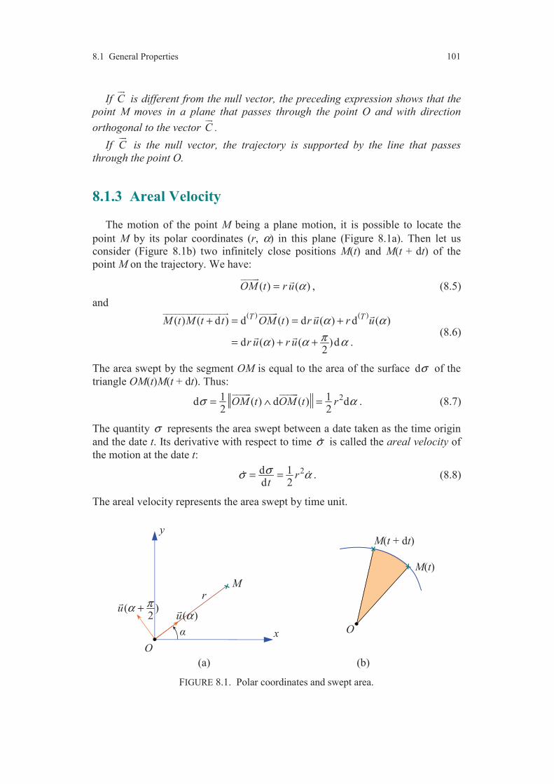
8.1 General Properties 101
If C
is different from the null vector, the preceding expression shows that the
point M moves in a plane that passes through the point O and with direction
orthogonal to the vector C
.
If C
is the null vector, the trajectory is supported by the line that passes
through the point O.
8.1.3 Areal Velocity
The motion of the point M being a plane motion, it is possible to locate the
point M by its polar coordinates (r, α) in this plane (Figure 8.1a). Then let us
consider (Figure 8.1b) two infinitely close positions M(t) and M(t + dt) of the
point M on the trajectory. We have:
( ) ( )OM t r u α=
, (8.5)
and ( ) ( )
( ) ( d ) d ( ) d ( ) d ( )
d ( ) ( )d .2
T TM t M t t OM t r u r u
r u r u
α α
πα α α
+ = = +
= + +
(8.6)
The area swept by the segment OM is equal to the area of the surface dσ of the
triangle OM(t)M(t + dt). Thus:
21 1d ( ) d ( ) d2 2
OM t OM t rσ α= ∧ =
. (8.7)
The quantity σ represents the area swept between a date taken as the time origin
and the date t. Its derivative with respect to time σ is called the areal velocity of
the motion at the date t:
2d 1d 2
rtσσ α= = . (8.8)
The areal velocity represents the area swept by time unit.
FIGURE 8.1. Polar coordinates and swept area.
O
M(t + dt)
M(t)
(b) (a)
x
M
y
r
( )u α( )
2u πα +
O

102 Chapitre 8 Motion with Central Acceleration
8.1.4 Area Law
In the case of a plane motion, the velocity vector of the point M is written from
(6.35):
( ) ( , ) ( ) ( )
2T M t r u r u πα α α= + +
. (8.9)
It results that Relation (8.4) leads to the following expression of the vector C
:
2C r k C kα= =
, (8.10)
while stating:
2C r α= . (8.11)
The vector C
being independent of time, it results from it that C is also inde-
pendent of time. Moreover, by comparing with Expression (8.8), we obtain:
dd 2
Ctσσ = = . (8.12)
The constant C is then called the area constant.
For a plane motion with central acceleration of centre O, the areal velocity
relatively to the point O is constant.
8.1.5 Expressions of the Kinematic Vectors
The kinematic vectors (6.29) and (6.33) can be expressed while introducing the
area constant C expressed by (8.11). We have:
( )
( ) ( )
2
2 2
2 2 2
22
2
d d d d d d 1 ,d d d d d d
d d d d 1 d 1 ,d d d d d
, .
r r r C rr Ct t rr
r r C Cr Ct r rr r
C Cr rr r
α αα α α α
αα α α α
α α
= = = = = −
= = = − = −
= =
(8.13)
Hence:
( ) ( )
d 1( , ) ( ) ( )d 2
T CM t C u ur r
πα αα
= − + + , (8.14)
( ) ( )
2 2
2 2
1 d 1( , ) ( )d
T Ca M t ur rr
αα
= − +
. (8.15)
8.1.6 Polar Equation of the Trajectory
In the case of a motion with central acceleration, Expression (8.1) of the
acceleration vector is written as:

8.1 General Properties 103
( ) ( , ) ( , ) ,Ta M t r OMλ α=
(8.16)
where λ is a real number which depends a priori of r and α. The equations of
Dynamics (Part V) will make it possible to derive the expression for λ.
By introducing, into Relation (8.16), Expressions (8.5) of the position vector
and (8.15) of the acceleration vector, we obtain the differential equation which
relates the variables r and α :
( )2
3
2 2
d 1 1 0d
rr rC
λα
+ + = . (8.17)
This equation allows us to obtain r as a function of α, thus:
( )r f α= , (8.18)
when λ is known. The time law of the motion along the trajectory is then derived
from (8.11) in the form:
[ ]221 1d d ( ) dt r fC C
α α α= = . (8.19)
If α0 is the value of α at the date t0, the expression of t is obtained as:
[ ]0
20
1 ( ) dt t fC
α
αα α− = . (8.20)
8.1.7 Motions with Central Acceleration for which ( ) 2( , )Ta M t OMω= −
The case of rectilinear motions has been studied in Subsection 7.1.4, and we
thus study in this subsection only the case of curvilinear motions. Let (x, y, 0) be
the Cartesian coordinates of the point M in the plane (Oxy). The coordinates (x, y)
check the relations:
2 2 and x x y yω ω= − = − . (8.21)
Whence, the equations of motion:
cos sin ,
cos sin ,
0.
x A t B t
y D t E t
z
ω ω
ω ω
= +
= +
=
(8.22)
We choose a time scale such as at the date 0,t = the point M is in M0 such as:
0 0 ,OM x i=
(8.23)
with a velocity:
0 0 0 .x i y j= + (8.24)
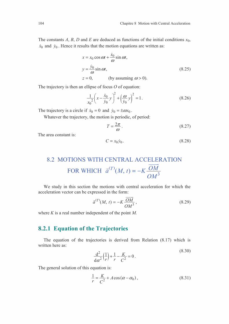
104 Chapitre 8 Motion with Central Acceleration
The constants A, B, D and E are deduced as functions of the initial conditions x0,
0x and 0y . Hence it results that the motion equations are written as:
00
0
cos sin ,
sin ,
0, (by assuming 0).
xx x t t
yy t
z
ω ωω
ωω
ω
= +
=
= >
(8.25)
The trajectory is then an ellipse of focus O of equation:
( )2 2
02
0 00
1 1x
x y yy yx
ω − + =
. (8.26)
The trajectory is a circle if 0 0x = and 0 0y xω= ± .
Whatever the trajectory, the motion is periodic, of period:
2T πω
= . (8.27)
The area constant is:
0 0C x y= . (8.28)
8.2 MOTIONS WITH CENTRAL ACCELERATION
FOR WHICH ( )
3( , )T OMa M t K
OM= −
We study in this section the motions with central acceleration for which the
acceleration vector can be expressed in the form:
( )
3( , )T OMa M t K
OM= −
, (8.29)
where K is a real number independent of the point M.
8.2.1 Equation of the Trajectories
The equation of the trajectories is derived from Relation (8.17) which is
written here as:
( )2
2 2
d 1 1 0d
Kr r Cα
+ − = .
(8.30)
The general solution of this equation is:
( )02
1 cosK Ar C
α α= + − , (8.31)

8.2 Motions with Central Acceleration for which ( )
3( , )
T OMa M t KOM
= −
105
where A and α0 are positive or negative constants determined by the initial condi-
tions (conditions at a given date). The preceding equation can be rewritten in the
form:
( )2
02
1 1 cosK ACr KC
α α = + −
. (8.32)
We observe then that the form of this equation is not changed, when we substitute
for the couple of constants ( )0, A α the couple ( )0, A α π− + . Without restricting
the generality of the study, it is then possible to choose the quantity 2AC
K as
positive. We state: 2
, with 0ACe eK
= ≥ . (8.33)
The equation of the trajectory is thus written finally as:
( )[ ]02
1 1 cosK er C
α α= + − . (8.34)
The trajectory of Equation (8.34) is derived from the curve of polar equation:
[ ]2
1 1 cosK er C
α= + , (8.35)
by applying to it a rotation of centre O and angle α0. Equation (8.35) is the polar
equation of a conic (ellipse, parabola, or hyperbola) of eccentricity e and para-
meter: 2Cp
K= . (8.36)
The origin O is one of the foci of the conic and the axis Ox
is the axis of the
conic. Equation (8.34) thus represents a conic of focus O, the axis of which forms
an angle α0 with the axis Ox
. However the condition 0r > imposes some res-
trictions according to the sign of K.
8.2.2 Study of the Trajectories
8.2.2.1 Case where K > 0
The parameter of the conic is then written as:
2CpK
= , (8.37)
and Equation (8.34) of the trajectory becomes:
( )01 cos
pr
e α α=
+ −. (8.38)

106 Chapitre 8 Motion with Central Acceleration
FIGURE 8.2. Trajectories in the case where K > 0.
1. If 1e > , the trajectory is the branch of hyperbola which turns its concavity
towards O (Figure 8.2a). The point P of smaller polar radius is called the peri-
centre:
1p
pOP r
e= =
+. (8.39)
2. If 1e = , the trajectory is a parabola (Figure 8.2b). The pericentre is then
defined by:
2p
pOP r= = . (8.40)
3. If 0 1e< < , the trajectory is an ellipse (Figure 8.2c). The pericentre is given
by:
1p
pOP r
e= =
+. (8.41)
The point A the most far from O is called the apocentre :
1A
pOA r
e= =
−. (8.42)
4. If 0e = , the trajectory is a circle of centre O.
conicaxis
x
y
P
p
O 0
asymptote
X
(a) 1e >
y
conicaxis
x
X P
p
O 0
(b) 1e =
x
conic axis
y
X P
p
O
0
A
C
Y
(c) 0 1e< <

8.2 Motions with Central Acceleration for which ( )
3( , )
T OMa M t KOM
= −
107
FIGURE 8.3. Trajectory in the case where K < 0.
8.2.2.2 Case where K < 0
When K is negative, the parameter of the conic is:
2CpK
= − , (8.43)
and Equation (8.34) of the trajectory is put in the form:
( )01 cos
pr
e α α−
=+ −
. (8.44)
The condition that r is positive imposes that the eccentricity e is higher than 1.
The trajectory is the branch of hyperbola (figure 8.3), which turns its convex part
towards O. The pericentre is defined by:
1p
pOP r
e= =
−. (8.45)
8.2.3 Velocity Magnitude at a Point of the Trajectory
We denote by the velocity vector
( )( , )T M t
at a point of the trajectory.
From Expression (8.14), we have:
( )2 2
2 2
2
d 1d
CCr rα
= +
. (8.46)
Whence, while introducing Expression (8.34) of 1r
, we obtain:
( )2
2 2
22 1K K e
r C= + −
, (8.47)
conic axis
x
y
X P O
0
asymptote

108 Chapitre 8 Motion with Central Acceleration
or
( )2 2 K Er
= + , (8.48)
setting:
( )2
2
2
1 12
KE eC
= − . (8.49)
We thus find that the quantity 2
2Kr
− remains constant during the motion. Thus:
2
2K Er
− = . (8.50)
The sign of E depends (8.49) only on the eccentricity of the conic:
— if the trajectory is an ellipse, 0E < ;
— if the trajectory is a parabola, 0E = ;
— if the trajectory is a hyperbola, 0E > .
8.2.4 Elliptic Motion. Kepler’s Laws
8.2.4.1 Characteristics of the Elliptic Trajectory
In the case of an elliptic trajectory, the equation of the trajectory is given by
Relation (8.38), with 0 1e≤ ≤ . The distance between the pericentre and the
apocentre is equal to the major axis 2a of the ellipse. Whence, from (8.41) and
(8.42) :
21
pa
e=
−. (8.51)
The distance c between the centre C of the ellipse (Figure 8.2c) and the focus O,
called focal distance is:
21
pec a OP
e= − =
−. (8.52)
Whence, the expression of the eccentricity:
cea
= . (8.53)
In the axis system (CXY) of the ellipse (Figure 8.2c), Equation (8.35) of the ellipse
is written as:
( )1
2 2 2p eX X Y= + + , (8.54)
or while expending:
( )2 2
2 21X ae Y
a b
+ + = , (8.55)

8.2 Motions with Central Acceleration for which ( )
3( , )
T OMa M t KOM
= −
109
with
( )2 2 21b a e= − . (8.56)
The parameter b represents the semi-minor axis of the ellipse.
Lastly, Expression (8.49) shows that the constant E is expressed in the case of
an elliptic trajectory in the form:
2KEa
= − . (8.57)
Hence it results that the magnitude of the velocity (8.48) is written as:
( )2 2 1Kr a
= − . (8.58)
The velocity is thus maximum at the pericentre (point nearest to the focus) and
minimum to the apocentre (the most distant point).
8.2.4.2 Periodic Time
The areal velocity being constant, the motion of the point M along the elliptic
trajectory is periodic of period T, equal to the time required by the point to
describe its trajectory. Thus, from Expression (8.12):
12
ab C Tπ = . (8.59)
By taking account of Relations (8.37), (8.51) and (8.56), the period of revolution
is written:
3/22T aK
π= . (8.60)
8.2.4.3 Kepler’s Laws
The Kepler’s laws regroup some of the results established in this chapter, and
may be stated as follows:
If, relatively to a reference system, a point M has a central acceleration
relatively to a point O fixed in this reference and if the trajectory of M has no
infinite branch, it results that:
1. The trajectory of the point M is an ellipse with the point O located at one of
its foci.
2. The areal velocity of the point relatively to the point O is constant.
3. The square of the periodic time is proportional to the cube of the semi-major
axis of the ellipse.
These laws were formulated in equivalent forms by the astronomer Kepler
(1571-1630), starting from astronomical observations of the motions of the
planets.

110 Chapitre 8 Motion with Central Acceleration
COMMENTS
A particularly important application of the motions with central accele-
ration is that of the motions of the planets and the motion of the Earth.
These motions of which the trajectories are ellipses are governed by the
Kepler’s laws introduced in this chapter. The reader will be thus more
particularly interested by the results established in Section 8.2.4. These
results will be used in Chapter 19.
CHAPTER 9
Kinematics of Rigid Body
9.1 GENERAL CONSIDERATIONS
9.1.1 Notion of Rigid Body
The purpose of the Mechanics of Rigid Bodies is to study the motions of
bodies, such that the distance between two arbitrary points of a given body is
independent of time or at least varies very little according to time. Such bodies are
called solid bodies, rigid bodies, or simply solids, and do not deform. Actual
structures or machines, however, are never absolutely rigid and deform under the
loads to which they are subjected. But these deformations are usually small and do
not appreciably affect the conditions of motions. The Mechanics of Rigid Bodies
allows us to describe the global behaviour of solids. The analysis of deformations
then requires us to consider theories which take into account the deformability of
bodies (resistance of materials, mechanics of deformable solids, etc.).
A rigid body will thus be described as a set of points constituting a geometric
space (Chapter 2) and such that the distance between two arbitrary points (P and
Q for example) of the body is independent of time:
( ) ( ), ( ) ( ) ( ) constantd P t Q t P t Q t= =
. (9.1)
9.1.2 Locating a Rigid Body
To know the motion of a rigid body relatively to a reference system, that is to
know the motion (position and kinematic vectors at any time) of each point of the
body. This problem constitutes the object of the Kinematics of Rigid Body.
To solve this problem, it is first necessary to express how it is possible to des-
cribe the situation of the body considered.
To situate a solid (S) relatively to a given reference system (T) (Figure 9.1), it
is necessary to know in the general case:
— the position, relatively to the reference (T), of a particular point of solid (S),
— the orientation of the solid (S) relatively to the reference (T).
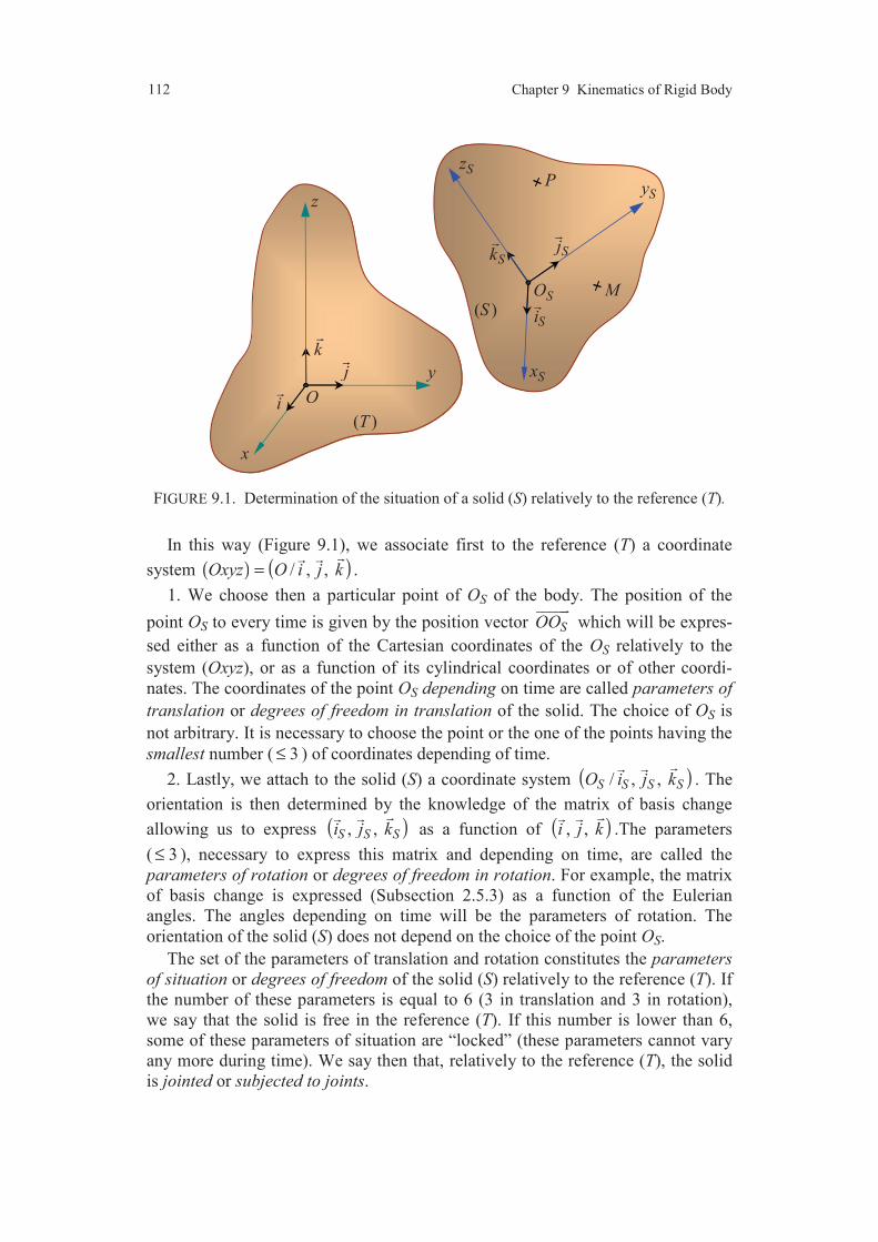
Chapter 9 Kinematics of Rigid Body 112
FIGURE 9.1. Determination of the situation of a solid (S) relatively to the reference (T).
In this way (Figure 9.1), we associate first to the reference (T) a coordinate
system ( ) ( )/ , , Oxyz O i j k=
.
1. We choose then a particular point of OS of the body. The position of the
point OS to every time is given by the position vector SOO
which will be expres-
sed either as a function of the Cartesian coordinates of the OS relatively to the
system (Oxyz), or as a function of its cylindrical coordinates or of other coordi-
nates. The coordinates of the point OS depending on time are called parameters of
translation or degrees of freedom in translation of the solid. The choice of OS is
not arbitrary. It is necessary to choose the point or the one of the points having the
smallest number ( 3≤ ) of coordinates depending of time.
2. Lastly, we attach to the solid (S) a coordinate system ( )/ , , S S S SO i j k
. The
orientation is then determined by the knowledge of the matrix of basis change
allowing us to express ( ), , S S Si j k
as a function of ( ), , i j k
.The parameters
( 3≤ ), necessary to express this matrix and depending on time, are called the
parameters of rotation or degrees of freedom in rotation. For example, the matrix
of basis change is expressed (Subsection 2.5.3) as a function of the Eulerian
angles. The angles depending on time will be the parameters of rotation. The
orientation of the solid (S) does not depend on the choice of the point OS.
The set of the parameters of translation and rotation constitutes the parameters
of situation or degrees of freedom of the solid (S) relatively to the reference (T). If
the number of these parameters is equal to 6 (3 in translation and 3 in rotation),
we say that the solid is free in the reference (T). If this number is lower than 6,
some of these parameters of situation are “locked” (these parameters cannot vary
any more during time). We say then that, relatively to the reference (T), the solid
is jointed or subjected to joints.
Oi
j
k
y
z
x
(T )
P zS
yS
OS
xS
Sj
Si
Sk
M (S )
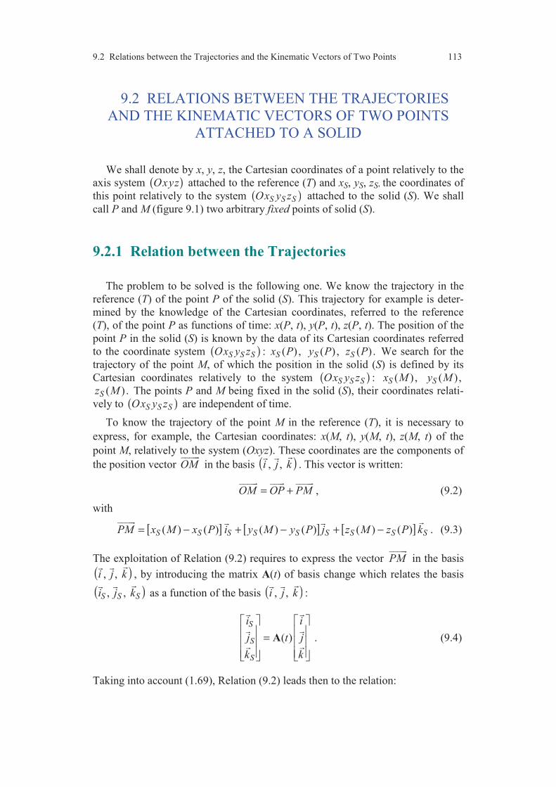
9.2 Relations between the Trajectories and the Kinematic Vectors of Two Points 113
9.2 RELATIONS BETWEEN THE TRAJECTORIES
AND THE KINEMATIC VECTORS OF TWO POINTS
ATTACHED TO A SOLID
We shall denote by x, y, z, the Cartesian coordinates of a point relatively to the
axis system ( )Oxyz attached to the reference (T) and xS, yS, zS, the coordinates of
this point relatively to the system ( )S S SOx y z attached to the solid (S). We shall
call P and M (figure 9.1) two arbitrary fixed points of solid (S).
9.2.1 Relation between the Trajectories
The problem to be solved is the following one. We know the trajectory in the
reference (T) of the point P of the solid (S). This trajectory for example is deter-
mined by the knowledge of the Cartesian coordinates, referred to the reference
(T), of the point P as functions of time: x(P, t), y(P, t), z(P, t). The position of the
point P in the solid (S) is known by the data of its Cartesian coordinates referred
to the coordinate system ( )S S SOx y z : ( ) ,Sx P ( ) ,Sy P ( ) .Sz P We search for the
trajectory of the point M, of which the position in the solid (S) is defined by its
Cartesian coordinates relatively to the system ( )S S SOx y z : ( ) ,Sx M ( ),Sy M
( ) .Sz M The points P and M being fixed in the solid (S), their coordinates relati-
vely to ( )S S SOx y z are independent of time.
To know the trajectory of the point M in the reference (T), it is necessary to
express, for example, the Cartesian coordinates: x(M, t), y(M, t), z(M, t) of the
point M, relatively to the system (Oxyz). These coordinates are the components of
the position vector OM
in the basis ( ), , i j k
. This vector is written:
OM OP PM= +
, (9.2)
with
[ ] [ ] [ ] ( ) ( ) ( ) ( ) ( ) ( )S S S S S S S S SPM x M x P i y M y P j z M z P k= − + − + −
. (9.3)
The exploitation of Relation (9.2) requires to express the vector PM
in the basis
( ), , i j k
, by introducing the matrix A(t) of basis change which relates the basis
( ), , S S Si j k
as a function of the basis ( ), , i j k
:
( )
S
S
S
i i
j t j
k k
=
A
. (9.4)
Taking into account (1.69), Relation (9.2) leads then to the relation:

Chapter 9 Kinematics of Rigid Body 114
t
( , ) ( , ) ( ) ( )
( , ) ( , ) ( ) ( ) ( )
( , ) ( , ) ( ) ( )
S S
S S
S S
x M t x P t x M x P
y M t y P t t y M y P
z M t z P t z M z P
− = + − −
A . (9.5)
trajectory of M trajectory of P transposed matrix coordinates of
in the reference (T) in the reference (T) of basis change M and P in (S)
This relation is the same as Relation (2.51) of reference change.
9.2.2 Relation between the Velocity Vectors
The velocity vector of the point M relatively to the reference (T) is:
( )( )
d( , )d
TT M t OM
t=
. (9.6)
In the same way, the velocity vector of the point P relatively to the reference (T) is
written as:
( )( )
d( , )d
TT P t OP
t=
. (9.7)
By substituting Expression (9.2) of OM
into Expression (9.6) of the velocity
vector, we obtain:
( )( ) ( )
( )( )
d d d( , ) ( , )d d d
T T TT TM t OP PM P t PM
t t t= + = +
. (9.8)
From expression (9.3), we have:
( )
[ ]( )
[ ]( )
[ ]( )
d d d( ) ( ) ( ) ( )d d d
d( ) ( ) .d
T T T
S S S S S S
T
S S S
PM x M x P i y M y P jt t t
z M z P kt
= − + −
+ −
(9.9)
Expressions (3.42) and (3.44) derived in Chapter 3 show that it is possible to write
the derivatives of the vectors of the basis in the forms:
( )( )
( )( )
( )( )
d d d, , .d d d
T T TT T T
S S S S S S S S Si i j j k kt t t
ω ω ω= × = × = ×
By substituting these expressions into (9.9), we obtain:
( )( )d
d
TT
SPM PMt
ω= ×
. (9.10)
Whence, the relation between the velocity vectors:
( ) ( ) ( ) ( , ) ( , )T T T
SM t P t PMω= + ×
. (9.11)
The vector ( )TSω
is called the instantaneous rotation vector relatively to the
motion of solid (S) with respect to the reference (T).
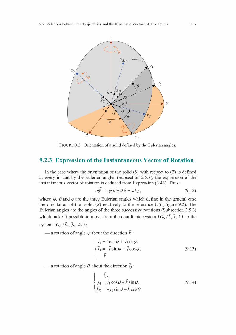
9.2 Relations between the Trajectories and the Kinematic Vectors of Two Points 115
FIGURE 9.2. Orientation of a solid defined by the Eulerian angles.
9.2.3 Expression of the Instantaneous Vector of Rotation
In the case where the orientation of the solid (S) with respect to (T) is defined
at every instant by the Eulerian angles (Subsection 2.5.3), the expression of the
instantaneous vector of rotation is deduced from Expression (3.43). Thus: ( )
3T
S Sk i kω ψ θ ϕ= + + , (9.12)
where ψ, θ and ϕ are the three Eulerian angles which define in the general case
the orientation of the solid (S) relatively to the reference (T) (Figure 9.2). The
Eulerian angles are the angles of the three successive rotations (Subsection 2.5.3)
which make it possible to move from the coordinate system ( )/ , , SO i j k
to the
system ( )/ , , S S S SO i j k
:
— a rotation of angle ψ about the direction k
:
3
3
cos sin ,
sin cos ,
,
i i j
j i j
k
ψ ψ
ψ ψ
= +
= − +
(9.13)
— a rotation of angle θ about the direction 3i
:
3
4 3
3
,
cos sin ,
sin cos ,S
i
j j k
k j k
θ θ
θ θ
= + = − +
(9.14)
x
Oi
k
y
y3
3j
3i
x3
j
Sk
Si
4j
xS
Sj
y4
yS
zS
z

Chapter 9 Kinematics of Rigid Body 116
— a rotation of angle ϕ about the direction Sk
:
3 4
3 4
cos sin ,
sin cos ,
,
S
S
S
i i j
j i j
k
ϕ ϕ
ϕ ϕ
= +
= − +
(9.15)
The components (9.12) of the rotation vector ( )TSω
thus correspond to the three
rotations.
The expression of the rotation vector in the basis ( ), , i j k
is deduced from
(9.12) by expressing the vectors 3i
and Sk
. Thus, from (9.13) and (9.14):
( )3 cos sin ,
sin cos sin cos .S
i i j
k i j k
ψ ψ
ψ ψ θ θ
= +
= − + +
Whence, the expression of the rotation vector:
( ) ( ) ( ) ( )cos sin sin sin cos sin cos .TS i j kω θ ψ ϕ ψ θ θ ψ ϕ ψ θ ψ ϕ θ= + + − + +
(9.16)
In the same way, it is possible to express the rotation vector in the basis
( ), , S S Si j k
. We obtain:
( ) ( ) ( ) ( )cos sin sin cos sin sin cos .TS S S Si j kω θ ϕ ψ ϕ θ ψ ϕ θ θ ϕ ϕ ψ θ= + + − + +
(9.17)
9.2.4 Kinematic Torsor
Let us compare Relation (9.11) of the velocity vectors of the points M and P:
( ) ( ) ( ) ( , ) ( , )T T T
SM t P t PMω= + ×
,
with the relation expressing the moments of a torsor at the points M and P:
M P R PM= + ×
.
We observe that there is identity of the structure of these relations. This identity
shows that it is thus possible to consider:
The velocity vector of a point M as being the moment at the point M of a
torsor, which will denote by ( ) TS , of which the resultant is the instantaneous
rotation vector ( )TSω
relative to the motion of the solid (S) with respect to the
reference (T).
The torsor ( ) TS thus introduced is called the kinematic torsor or velocity
distributor torsor, relative to the motion of the solid (S) with respect to the
reference (T). Its elements of reduction at point M are:

9.2 Relations between the Trajectories and the Kinematic Vectors of Two Points 117
( )( )T TSSR ω=
, instantaneous rotation vector; (9.18)
( )( )( , )
T TM S M t=
, velocity vector of the point M of (S). (9.19)
The relation between the velocity vectors is then obtained in the inverse way
according to the relation of the moments of a torsor:
( ) ( ) ( )T T TM PS S SR PM= + ×
, (9.20)
or taking account of (9.18) and (9.19):
( ) ( ) ( ) ( , ) ( , )T T T
SM t P t PMω= + ×
, (9.21)
which is the initial relation (9.11). The two formalisms, one of mathematical
nature and the other of mechanical nature, will not have to be mixed within a same
relation.
If the elements of reduction of the kinematic torsor are expressed at the
particular point OS chosen to define the parameters of situation of the solid (Sub-
section 9.1.2), its resultant (rotation vector) depends only on the parameters of
rotation and its moment (velocity vector of the point OS) depends only on the
parameters of translation. There is decoupling between the parameters of trans-
lation and rotation. Moreover, the kinematic torsor entirely characterizes the
motion of the solid (S) relatively to the reference (T), with regard of the velocity
vectors, whence its interest.
9.2.5 Relation between the Acceleration Vectors
The relation between the acceleration vectors is obtained by deriving Expres-
sion (9.11). That is:
( )( )
( )
( )( )
( )( ) ( )
( )
d( , ) ( , )d
d d d( , ) .d d d
TT T
T T TT T T
S S
a M t M tt
P t PM PMt t t
ω ω
=
= + × + ×
(9.22)
The first term is the acceleration vector of the point P. The third term is expressed
using Relation (9.10). Furthermore, it is possible to show that:
( )( )
( )( ) ( )
d d , vector which we shall denote by .d d
T ST T T
S S St t
ω ω ω=
(9.23)
The rotation vector thus has the same derivative relatively to (T) and (S). Finally,
Expression (9.22) leads to the relation between the acceleration vectors:
( ) ( ) ( ) ( ) ( )( ) ( , ) ( , )T T T T TS S Sa M t a P t PM PMω ω ω= + × + × ×
. (9.24)
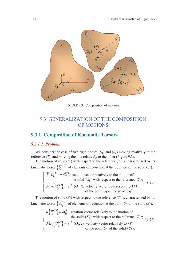
Chapter 9 Kinematics of Rigid Body 118
FIGURE 9.3. Composition of motions.
9.3 GENERALIZATION OF THE COMPOSITION
OF MOTIONS
9.3.1 Composition of Kinematic Torsors
9.3.1.1 Problem
We consider the case of two rigid bodies (S1) and (S2) moving relatively to the
reference (T), and moving the one relatively to the other (Figure 9.3).
The motion of solid (S1) with respect to the reference (T) is characterized by its
kinematic torsor ( ) 1
TS of elements of reduction at the point O1 of the solid (S1):
( ) ( )
( ) ( )
( ) ( ) ( )
( )
1 1
1 1
1
1
1 1
, rotation vector relatively to the motion of
the solid with respect to the reference ;
( , ), velocity vector with respect to
of the point of the solid .
T TS S
T TO S
R
S T
O t T
O S
ω =
=
(9.25)
The motion of solid (S2) with respect to the reference (T) is characterized by its
kinematic torsor ( ) 2
TS of elements of reduction at the point O2 of the solid (S2):
( ) ( )
( ) ( )
( ) ( ) ( )
( )
2 2
2 2
2
2
2 2
, rotation vector relatively to the motion of
the solid with respect to the reference ;
( , ), velocity vector relatively to
of the point of the solid .
T TS S
T TO S
R
S T
O t T
O S
ω =
=
(9.26)
Oi
j
k
y
z
x
(T )
z2
y2
O2x2
2j
2i
2k
(S2 )
M
z1
y1
O1
1j
1i
1k
(S1 )
x1
9.3 Generalization of the Composition of Motions 119
Lastly, the motion of the solid (S2) relatively to the solid (S1) is characterized
by its kinematic torsor ( ) 1
2
SS of elements of reduction at the point O2 of the
solid (S2):
( ) ( )
( ) ( )( ) ( ) ( )
( )
1 1
2 2
1 12 2
2 1
2 1
2 2
, rotation vector relatively to the motion of
the solid with respect to the solid ;
( , ), velocity vector relatively to
of the point of the solid .
S SS S
S SO S
R
S S
O t S
O S
ω =
=
(9.27)
9.3.1.2 Relation between the Moment Vectors
The velocity vector relatively to the reference (T) of the point O2 of the solid
(S2) is written:
( )( ) ( )
( ) ( )( )
2 12 1 1 12 2d d d( , ) ( , )d d d
T T TT TO t OO OO O O O t O O
t t t= = + = +
. (9.28)
If we introduce the coordinates x1(O2, t), y1(O2, t) and z1(O2, t) of the point O2
with respect to a coordinate system attached to (S1) , we have:
1 1 2 1 1 2 1 1 2 12 ( , ) ( , ) ( , )O O x O t i y O t j z O t k= + +
. (9.29)
Whence:
( )
( ) ( ) ( )
1 1 2 1 1 2 1 1 2 12
11 11 2 1 2 1 2
d( , ) ( , ) ( , )
d
dd d ( , ) ( , ) ( , ) ,
d d d
T
TT T
O O x O t i y O t j z O t kt
ji kx O t y O t z O t
t t t
= + +
+ + +
or by analogy with (9.9) and (9.10)
( )( ) ( )
1
11 2 12 2
d( , )
d
TS T
SO O O t O O
tω= + ×
. (9.30)
Thus, by substituting into Relation (9.28:
( ) ( ) ( ) ( )
1
12 2 1 1 2( , ) ( , ) ( , )T S T T
SO t O t O t O Oω= + + ×
. (9.31)
However, we have the relation: ( ) ( ) ( ) 21 1
1 1 2( , )T T TOS S
O t O Oω+ × =
. (9.32)
Relation (9.31), by taking account of (9.26), (9.27) and (9.32), is thus written
finally in the form: ( ) ( ) ( ) 1
2 2 22 2 1
ST TO O OS S S
= +
. (9.33)
9.3.1.3 Relation between the Resultants
Let us consider a point M of the solid (S2) (Figure 9.3). We may write:
Chapter 9 Kinematics of Rigid Body 120
( ) ( ) ( ) ( )
2 22 2( , ) ( , )T T T T
M S SM t O t O Mω= = + ×
, (9.34)
and
( ) ( ) ( ) ( )
1 11 1
2 22 2( , ) ( , )
S SS SM S S
M t O t O Mω= = + × . (9.35)
Furthermore, by applying Relation (9.31) at the point M of the solid (S2) (instead
of the point O2), we obtain:
( ) ( ) ( ) ( )
1
11 2( , ) ( , ) ( , )
ST T TS
M t M t O t O Mω= + + ×
. (9.36)
Combination of Expressions (9.36) and (9.31) leads to:
( ) ( ) ( ) ( ) ( )
1 1
12 2 2( , ) ( , ) ( , ) ( , )
S ST T TS
M t O t M t O t O Mω− = − + ×
, (9.37)
or by taking account of Relations (9.34) and (9.35):
( ) ( ) ( )1
2 2 12 2 2
ST TS S S
O M O M O Mω ω ω× = × + ×
.
We deduce from that the relation between the rotation vectors:
( ) ( ) ( )1
2 2 1
ST TS S S
ω ω ω= +
. (9.38)
9.3.1.4 Relation between the Kinematic Torsors
From the relations between the resultants (9.38) and moments (9.33) of the
kinematic torsors, we deduce the relation of the composition of motions:
( ) ( ) ( ) 1
2 2 1
ST TS S S
= + . (9.39)
motion of (S2) motion of (S2) motion of (S1)
relatively to (T) relatively to (S1) relatively to (T)
The preceding relation expresses the combination of motions. This relation can
be extended to an arbitrary number of rigid bodies:
( ) ( ) ( ) ( ) 1 1
2 1 . . . n
n n
S ST TS S S S
−= + + + . (9.40)
9.3.2 Inverse Motions
The motion of solid (S1) relatively to solid (S2) is called the inverse motion of
the motion of (S2) relatively to solid (S1).
By identifying the solid (S2) with the reference (T), Relation (9.39) is written:
( ) ( ) ( ) 1 2 2
2 1 20S S S
S S S+ = = . (9.41)

9.4 Examples of Solid Motions 121
Whence, the relation between the inverse motions:
( ) ( ) 1 2
2 1
S SS S
= − . (9.42)
In particular, it results that:
( ) ( )1 2
2 1.
S S
S Sω ω= −
(9.43)
The instantaneous rotation vectors of the two inverse motions are opposite.
9.4 EXAMPLES OF SOLID MOTIONS
9.4.1 Motion of Rotation about a Fixed Axis
9.4.1.1 Definition and Parameters of Situation
The motion of a solid (S) relatively to a reference (T) is a motion of rotation
about an axis, if and only if two points A and B, distinct, of the solid (S) remain
fixed in (T) during the motion (Figure 9.4a).
Because of the invariance of the distances, all the points of the body located on
the line AB remain also fixed. The line ( )AB ∆= is the axis of rotation of the
motion.
The examples of motions of rotation about an axis are multiple: rotor, wheel,
winch, pendulum, etc.
To locate the solid (S) relatively to the reference (T), we attach first the coor-
dinate system (Oxyz) to the reference (T) such as the axis Oz
coincides with the
axis (∆) of rotation (Figure 9.4b), then we search for the parameters of situation.
1. We choose a particular point of the solid (S): a point of the axis of rotation,
for example the point O. This point being fixed, the motion does not have any
parameter of translation.
2. We attach to the solid (S) a coordinate system: ( ) ,S SOx y z of the same
origin and with the same axis Oz
as the system ( ).Oxyz The orientation of this
coordinate system is characterized by the angle of rotation ψ about the axis Oz
:
( ) ( ) ( ) , ,S St i i j jψ = =
. (9.44)
The motion is finally characterized by one parameter of rotation ψ. The basis
change between the two coordinate systems is written as:
cos sin ,
sin cos ,
.
S
S
i i j
j i j
k
ψ ψ
ψ ψ
= +
= − +
(9.45)
We have:
( ), ( ),2
S Si u j uπψ ψ= = +
(9.46)

Chapter 9 Kinematics of Rigid Body 122
FIGURE 9.4. Motion of Rotation about a Fixed Axis.
and ( ) ( )
d d, ,
d d
T TS S
S Si j
j it t
ψ ψ= = −
(9.47)
9.4.1.2 Kinematic Torsor
The kinematic torsor ( ) TS relatively to the motion of rotation of the solid (S)
with respect to (T) is defined by its elements of reduction at the point O:
( ) ( )T TS SR kω ψ= =
, (9.48)
( ) ( )( , ) 0T T
O S O t= = . (9.49)
9.4.1.3 Kinematic Vectors of an Arbitrary Point
Let M be an arbitrary point of the solid (S) (Figure 9.4). Its position in (S) is
determined by the data of its Cartesian coordinates xS, yS, zS, relatively to the
system ( )S SOx y z :
S S S S SOM x i y j z k= + +
. (9.50)
The velocity vector of the point M can be obtained:
— either by deriving directly the position vector and using Relations (9.47):
( )( )
d( , )d
TT
S S S SM t OM x j y it
ψ ψ= = −
, (9.51)
y
A
B
(S )
( )
(a)
Oi
j
k
z
x (T )
zS
yS
Sj
Si
M
yS
(S )
( )
(b)
xS
xS

9.4 Examples of Solid Motions 123
— or by using Relation (9.21):
( ) ( ) ( )
( )
( , ) ( , )
.
T T TS
S S S S S
M t O t OM
k x i y j z k
ω
ψ
= + ×
= × + +
(9.52)
Whence:
( ) ( , )T
S S S SM t x j y iψ ψ= − .
The velocity vector can then be expressed in the basis ( ), , i j k
by considering
the basis change (9.45). Thus:
( ) ( ) ( ) ( , ) sin cos cos sinTS S S SM t x y i x y jψ ψ ψ ψ ψ ψ= − + + −
. (9.53)
The acceleration vector can then be obtained in different ways.
1. Starting from Relation (9.24) which is written:
( ) ( ) ( ) ( ) ( )( ) ( , ) ( , )T T T T TS S Sa M t a O t OM OMω ω ω= + × + × ×
,
with ( )
( ) ( )( ) ( )( ) ( )
2 2
( , ) 0,
,
T
TS S S S S S S S S S
T TS S S S S S S S S S
a O t
OM k x i y j z k x j y i
OM k x j y i x i y j
ω ψ ψ ψ
ω ω ψ ψ ψ ψ ψ
=
× = × + + = −
× × = × − = − −
Whence:
( ) ( ) ( )
2 2( , )TS S S S S Sa M t y x i x y jψ ψ ψ ψ= − + + −
. (9.54)
2. By deriving Expression (9.51) of the velocity vector:
( )( )
( )
2 2d( , ) ( , )d
TT T
S S S S S S S Sa M t M t x j x i y i y jt
ψ ψ ψ ψ= = − − − . (9.55)
We find Relation (9.54) again. The acceleration vector can thus be obtain from
(9.45) in the basis ( ), , i j k
:
( ) ( ) ( )
( ) ( )
2 2
2 2
( , ) cos sin
sin cos .
TS S S S
S S S S
a M t y x x y i
y x x y j
ψ ψ ψ ψ ψ ψ
ψ ψ ψ ψ ψ ψ
= − + + −
+ − + + −
(9.56)
3. Lastly, ( )
( , )Ta M t
can be deduced by deriving directly Expression (9.53):
( ) ( ) ( )
( ) ( )
2
2
( , ) sin cos cos sin
cos sin sin cos .
TS S S S
S S S S
a M t x y x y i
x y x y j
ψ ψ ψ ψ ψ ψ
ψ ψ ψ ψ ψ ψ
= − + + −
+ − − +
We obtain Relation (9.56) again.

Chapter 9 Kinematics of Rigid Body 124
9.4.2 Translation Motion of a Rigid Body
9.4.2.1 Definition and Parameters of Situation
A solid (S) has a translation motion relatively to the reference (T) if the solid
(S) has an invariable orientation during the time relatively to the reference (T).
It is equivalent to say that the basis ( ), , S S Si j k
attached to the solid (S) is
independent of time. It is then possible to choose the coordinate systems attached
to (S) and (T) so that their axes remain parallel (Figure 9.5) during the motion of
the solid (S):
, , .S S Si i j j k k= = =
(9.57)
To locate the solid (S) relatively to the reference (T), it is thus necessary and
sufficient to determine the position of a point OS of the solid (S), thus 3 para-
meters. The translation motion is a motion with 3 degrees of freedom in trans-
lation.
Note. We will denote in a similar way the axes of same direction. Thus, the
coordinate systems respectively attached to (T) and (S) are noted here by (Oxyz)
and (OSxyz). They differ simply by their origins.
The position relatively to the reference (T) of any point M of the solid (S) is
given by the position vector:
S SOM OO O M= +
, (9.58)
where SO M
is an invariable vector during the motion of the solid (S) relatively to
(T). Thus, it results that the trajectory of the point M in the reference (T) is
deduced from the one of OS, by the translation of vector SO M
: the trajectories of
FIGURE 9.5. Translation motion.
Oi
j
k
y
z
x
(T )
j
k
i OS (S )
M
z
y
x

9.4 Examples of Solid Motions 125
all the points of (S) are superposable curves. If the trajectory of the point OS is a
straight line, it is said that the solid (S) has a motion of rectilinear translation (the
number of parameters is reduced to 1). If its trajectory is a curved line, the motion
of the solid (S) is a curvilinear translation with 2 or 3 parameters de translation,
according as the curve is plane or not.
The examples of translation motion are numerous: slides (shaper, planer, etc.),
tables of machines-tools (milling machine, etc.), pistons, elevators, coupling
crank, etc.
9.4.2.2 Kinematic Torsor
The elements of reduction of the kinematic torsor( ) TS are written at the point
OS as: ( ) ( )
0T TS SR ω= =
, (9.59)
( ) ( )
( , )S
T TO S SO t=
. (9.60)
The expression of the velocity vector of the point OS depends on the translation
motion under consideration.
The translation motion is characterized by a null rotation vector and conse-
quently by a kinematic torsor which is a couple-torsor.
9.4.2.3 Kinematic Vectors of an Arbitrary Point
The kinematic torsor being a couple-torsor, its moment is the same at any point
M of the solid (S). So, it results that:
( ) ( ) ( , ) ( , ), ( ).T T
SM t O t M S= ∀ ∈ (9.61)
It is the same for the acceleration vector:
( ) ( ) ( , ) ( , ), ( ).T T
Sa M t a O t M S= ∀ ∈
(9.62)
In a motion of translation all the points of the rigid body have the same kinematic
vectors.
9.4.3 Motion of a Body Subjected to a Cylindrical Joint
9.4.3.1 Definition and Parameters of Situation
During its motion, a solid (S) is subjected to a cylindrical joint relatively to the
reference (T), if and only if a straight line attached to the solid (S) remains in
geometrical coincidence with a line attached to the reference (T).
The line (∆) attached to the reference (T) is called the axis of the cylindrical
joint. To define the parameters of situation, we associate the system (Oxyz) to the
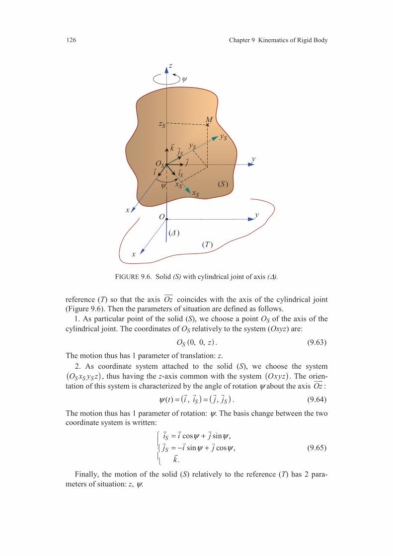
Chapter 9 Kinematics of Rigid Body 126
FIGURE 9.6. Solid (S) with cylindrical joint of axis (∆).
reference (T) so that the axis Oz
coincides with the axis of the cylindrical joint
(Figure 9.6). Then the parameters of situation are defined as follows.
1. As particular point of the solid (S), we choose a point OS of the axis of the
cylindrical joint. The coordinates of OS relatively to the system (Oxyz) are:
( )0, 0, SO z . (9.63)
The motion thus has 1 parameter of translation: z.
2. As coordinate system attached to the solid (S), we choose the system
( )S S SO x y z , thus having the z-axis common with the system ( )Oxyz . The orien-
tation of this system is characterized by the angle of rotation ψ about the axis Oz
:
( ) ( )( ) , , S St i i j jψ = =
. (9.64)
The motion thus has 1 parameter of rotation: ψ. The basis change between the two
coordinate system is written:
cos sin ,
sin cos ,
.
S
S
i i j
j i j
k
ψ ψ
ψ ψ
= +
= − +
(9.65)
Finally, the motion of the solid (S) relatively to the reference (T) has 2 para-
meters of situation: z, ψ.
z
OS
i
j
k
y
x
(T )
zS
yS
Sj
Si
M
yS
(S )
( )
x
yO
xSxS

9.4 Examples of Solid Motions 127
9.4.3.2 Kinematic Torsor
The kinematic torsor ( ) TS relatively to the motion of the solid (S) with
respect to the reference (T) has for elements of reduction at the point O:
( ) ( ),T T
S SR kω ψ= = (9.66)
( ) ( ) ( , ) .S
T TO S SO t z k= =
(9.67)
9.4.3.3 Kinematic Vectors of an Arbitrary Point
By comparing the kinematic torsor of a motion of a rigid body subjected to a
cylindrical joint with the one of the motion of rotation about a fixed axis (Rela-
tions (9.48) and (9.49)), we observe that these relations differ by the moment at
the point OS. It results from the expression of the moment at any point M:
( ) ( ) ( ) ( , ) ( , ) ,T T T
S S SM t O t O Mω= + ×
that the kinematic vectors of the motion with a cylindrical joint are deduced from
the relations obtained in the case of the rotation about an axis, by adding the trans-
lation terms:
( ) ( ) ( , ) , ( , )T T
S SO t z k a O t z k= = . (9.68)
Hence the expressions of the kinematic vectors:
( ) ( , )T
S S S SM t y i x j z kψ ψ= − + +
, (9.69)
( ) ( ) ( ) ( , ) sin cos cos sinT
S S S SM t x y i x y j z kψ ψ ψ ψ ψ ψ= − + + − +
, (9.70)
( ) ( ) ( )
2 2( , )TS S S S S Sa M t y x i x y j z kψ ψ ψ ψ= − + + − +
, (9.71)
( ) ( ) ( )
( ) ( )
2 2
2 2
( , ) cos sin
sin cos .
TS S S S
S S S S
a M t y x x y i
y x x y j z k
ψ ψ ψ ψ ψ ψ
ψ ψ ψ ψ ψ ψ
= − + + −
+ − + + − +
(9.72)
9.4.4 Motion of Rotation about a Fixed Point
9.4.4.1 Definition and Parameters of Situation
The motion of a solid (S) relatively to the reference (T) is a motion of rotation
about a fixed point, if and only if a point A of the solid (S) remain fixed in the
reference (T) during the motion.
The coordinate systems associated to (S) and (T) are chosen so that their origins
O and OS coincide with the point A (Figure 9.7). To locate the solid (S) relatively
to the reference (T), it is necessary and sufficient to determine the orientation of
(S), defined by the three Eulerian angles: ψ, θ and ϕ as functions of time. A
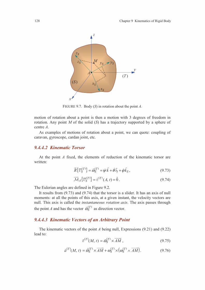
Chapter 9 Kinematics of Rigid Body 128
FIGURE 9.7. Body (S) in rotation about the point A.
motion of rotation about a point is then a motion with 3 degrees of freedom in
rotation. Any point M of the solid (S) has a trajectory supported by a sphere of
centre A.
As examples of motions of rotation about a point, we can quote: coupling of
caravan, gyroscope, cardan joint, etc.
9.4.4.2 Kinematic Torsor
At the point A fixed, the elements of reduction of the kinematic torsor are
written:
( ) ( ) 3
T TS S SR k i kω ψ θ ϕ= = + +
, (9.73)
( ) ( )( , ) 0T T
A S A t= = . (9.74)
The Eulerian angles are defined in Figure 9.2.
It results from (9.73) and (9.74) that the torsor is a slider. It has an axis of null
moments: at all the points of this axis, at a given instant, the velocity vectors are
null. This axis is called the instantaneous rotation axis. The axis passes through
the point A and has the vector ( )TSω
as direction vector.
9.4.4.3 Kinematic Vectors of an Arbitrary Point
The kinematic vectors of the point A being null, Expressions (9.21) and (9.22)
lead to: ( ) ( )
( , )T TSM t AMω= ×
, (9.75)
( ) ( ) ( ) ( )( )( , )T T T TS S Sa M t AM AMω ω ω= × + × ∧
. (9.76)
Ay
z
x
(T )
zS
yS
xS
M
xS
yS
(S )
zS
9.4 Examples of Solid Motions 129
The vector AM
is a vector independent of time in the system ( )S S SAx y z :
S S S S S SAM x i y j x k= + +
, (9.77)
where xS, yS and zS are the Cartesian coordinates of the point M relatively to the
reference ( ).S S SAx y z The product vectors are thus obtained simply by expres-
sing ( )TSω
in the basis ( ), , S S Si j k
. Hence:
( ) 1 2 3
TS S S Si j kω ω ω ω= + +
, (9.78)
with, from (9.17):
1
2
3
cos sin sin ,
cos sin sin ,
cos .
ω θ ϕ ψ ϕ θ
ω ψ ϕ θ θ ϕ
ω ϕ ψ θ
= +
= − = +
(9.79)
Whence:
( ) ( ) ( ) ( ) 2 3 3 1 1 2( , )T
S S S S S S S S SM t z y i x z j y x kω ω ω ω ω ω= − + − + −
. (9.80)
The determination of ( )
( , )Ta M t
needs to express ( )TSω . We obtain:
( ) 1 2 3
TS S S Si j kω ω ω ω= + +
, (9.81)
with
1
2
3
cos sin sin sin cos sin sin cos ,
cos sin sin sin cos cos sin cos ,
cos sin .
ω θ ϕ θϕ ϕ ψ ϕ θ ψϕ ϕ θ ψθ ϕ θ
ω ψ ϕ θ ψϕ ϕ θ ψθ ϕ θ θ ϕ θϕ ϕ
ω ϕ ψ θ ψθ θ
= − + + +
= − + − − = + −
(9.82)
It results from this that the acceleration vector is expressed in the form:
( ) ( ) ( ) ( )
( ) ( ) ( )
( ) ( ) ( )
2 22 3 1 2 3 1 2 2
2 23 1 2 3 1 1 2 3
2 21 2 1 3 2 2 3 1
( , )
.
TS S S S
S S S S
S S S S
a M t x y z i
y z x j
z x y k
ω ω ω ω ω ω ω ω
ω ω ω ω ω ω ω ω
ω ω ω ω ω ω ω ω
= − + + − + +
+ − + + − + +
+ − + + − + +
(9.83)
9.4.5 Plane Motion
9.4.5.1 Definition and Parameters of Situation
The motion of a solid (S) relatively to the reference (T) is a plane motion, if an
only if, a plane (PS) attached to the solid (S) remains in coincidence with a plane
(P) attached to the reference (T).
It is then always possible to choose (figure 9.8) the coordinate systems atta-
ched to (S) and (T), so that the plane ( )S SOx y is the plane (PS) and the plane
( )Oxy is the plane (P). The axes Oz
and SO z
have then the same direction k
.
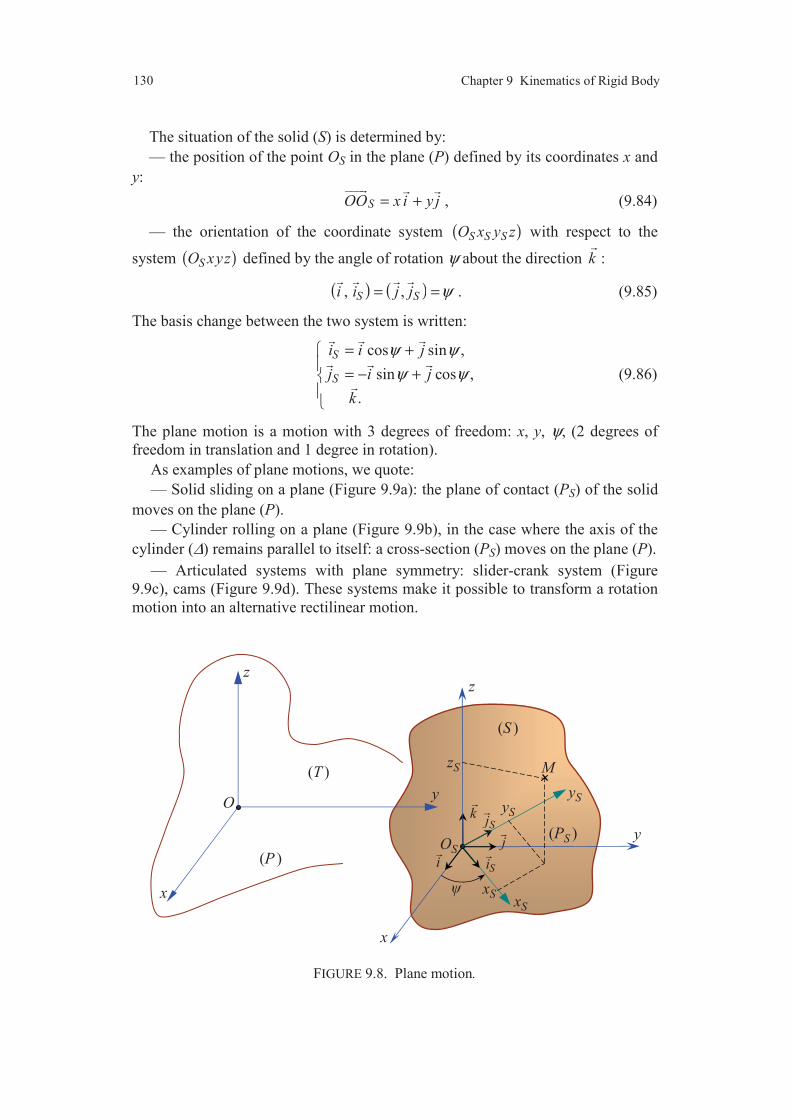
Chapter 9 Kinematics of Rigid Body 130
The situation of the solid (S) is determined by:
— the position of the point OS in the plane (P) defined by its coordinates x and
y:
SOO x i y j= +
, (9.84)
— the orientation of the coordinate system ( )S S SO x y z with respect to the
system ( )SO xyz defined by the angle of rotation ψ about the direction k
:
( ) ( ) , ,S Si i j j ψ= =
. (9.85)
The basis change between the two system is written:
cos sin ,
sin cos ,
.
S
S
i i j
j i j
k
ψ ψ
ψ ψ
= +
= − +
(9.86)
The plane motion is a motion with 3 degrees of freedom: x, y, ψ, (2 degrees of
freedom in translation and 1 degree in rotation).
As examples of plane motions, we quote:
— Solid sliding on a plane (Figure 9.9a): the plane of contact (PS) of the solid
moves on the plane (P).
— Cylinder rolling on a plane (Figure 9.9b), in the case where the axis of the
cylinder (∆) remains parallel to itself: a cross-section (PS) moves on the plane (P).
— Articulated systems with plane symmetry: slider-crank system (Figure
9.9c), cams (Figure 9.9d). These systems make it possible to transform a rotation
motion into an alternative rectilinear motion.
FIGURE 9.8. Plane motion.
z
OS
i
j
k
y
x
zS
yS
Sj
Si
M
yS
(PS )
(S )
xSxS
x
(P )
yO
z
(T )
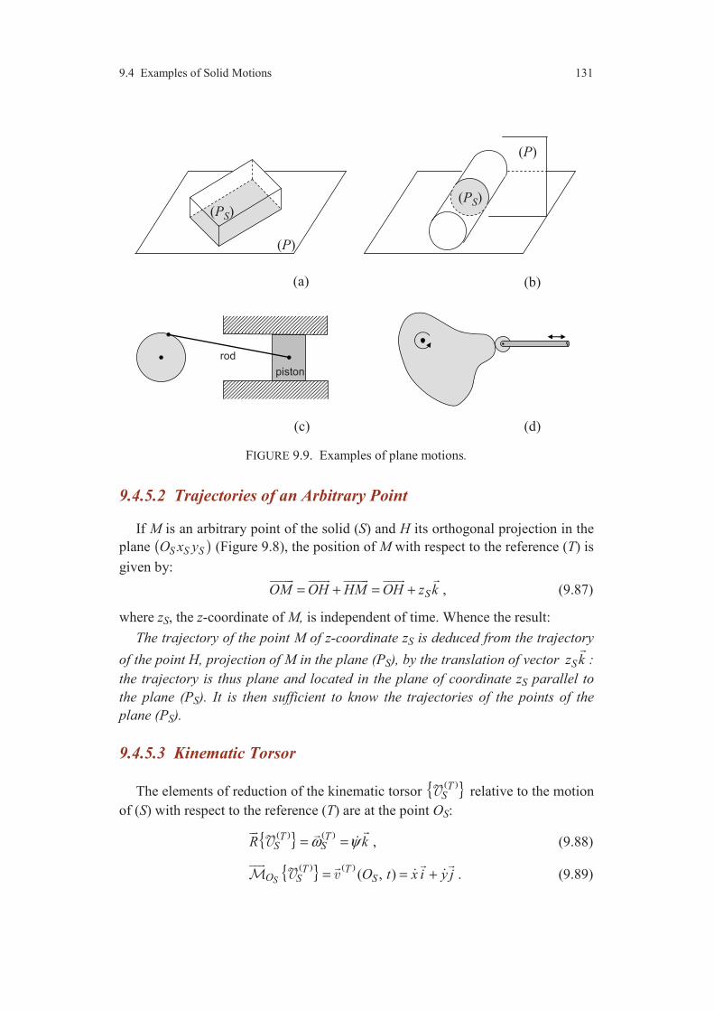
9.4 Examples of Solid Motions 131
FIGURE 9.9. Examples of plane motions.
9.4.5.2 Trajectories of an Arbitrary Point
If M is an arbitrary point of the solid (S) and H its orthogonal projection in the
plane ( )S S SO x y (Figure 9.8), the position of M with respect to the reference (T) is
given by:
SOM OH HM OH z k= + = +
, (9.87)
where zS, the z-coordinate of M, is independent of time. Whence the result:
The trajectory of the point M of z-coordinate zS is deduced from the trajectory
of the point H, projection of M in the plane (PS), by the translation of vector Sz k
:
the trajectory is thus plane and located in the plane of coordinate zS parallel to
the plane (PS). It is then sufficient to know the trajectories of the points of the
plane (PS).
9.4.5.3 Kinematic Torsor
The elements of reduction of the kinematic torsor ( ) TS relative to the motion
of (S) with respect to the reference (T) are at the point OS:
( ) ( )T TS SR kω ψ= =
, (9.88)
( ) ( ) ( , )S
T TO S SO t x i y j= = +
. (9.89)
(P)
(PS)
(a) (b)
(c) (d)
rod
piston
(P)
(PS)

Chapter 9 Kinematics of Rigid Body 132
9.4.5.4 Kinematic Vectors of an Arbitrary Point
Let M be an arbitrary point of the solid (S) of Cartesian coordinates xS, yS, zS,
relatively to the coordinate system ( )S S SO x y z :
S S S S SOM x i y j z k= + +
. (9.90)
The velocity vector is written:
( ) ( ) ( ) ( , ) ( , )T T T
S S SM t O t O Mω= + ×
. (9.91)
Thus: ( )
( , )TS S S SM t x i y j x j y iψ ψ= + + −
.
Or by taking account of (9.86):
( ) ( )[ ] ( )[ ] ( , ) sin cos cos sinTS S S SM t x x y i y x y jψ ψ ψ ψ ψ ψ= − + + + −
.
(9.92)
The acceleration vector is deduced from the preceding relation by derivation:
( ) ( ) ( )
( ) ( )
2
2
( , ) sin cos cos sin
cos sin sin cos .
TS S S S
S S S S
a M t x x y x y i
y x y x y j
ψ ψ ψ ψ ψ ψ
ψ ψ ψ ψ ψ ψ
= − + − −
+ + − − +
(9.93)
9.4.5.5 Instantaneous Centre of Rotation
The scalar invariant of the kinematic torsor of the plane motion is from (9.88)
and (9.89): ( ) ( ) ( )
( , ) 0T T TS S SI O tω= =⋅
. (9.94)
The kinematic torsor is thus a slider which has an instantaneous axis of rotation,
the points of which have null velocity vectors. This axis has ( )TSω
for direction
vector. It is thus orthogonal to the plane (Oxy), at a point I which depends of the
motion. This point I, belonging to the planes (P) and (PS), is called the
instantaneous centre of rotation of the motion of (S) with respect to (T) (or of the
plane (PS) with respect to the plane (P)). Its position is given by Expression (5.27)
which is written here:
( )
2
( , )TS
Sk O t
O Iψ
ψ
×=
. (9.95)
We have:
( )( ) ( )
d d( , )
d d
T TT
S SSO t OO OOt
ψψ
= =
.
It results that the position of the point I is expressed according to the relation: ( )
d
d
T
SSO I k OOψ
= ×
. (9.96)

9.4 Examples of Solid Motions 133
9.4.5.6 Space Centrode and Body Centrode
The instantaneous centre of rotation is a mobile point relatively to the refe-
rence (T) and relatively to the solid (S). We call then:
— space centrode of the motion of the plane (PS) on (P), the set of points of
the plane (P) in coincidence at every time with the instantaneous centre of rota-
tion: that is the trajectory of the centre of rotation in the reference (T);
— body centrode of the motion of the plane (PS) on (P), the set of points of the
plane (PS) in coincidence at every time with the instantaneous centre of rotation:
that is the trajectory of the centre of rotation in the reference (S).
Let us express the velocity vector of the point I relatively to the reference (T):
( )( )
d( , )
d
TT I t OI
t=
, (9.97)
with ( ) ( )
( ) ( )( )
d d d( , )
d d d
T T TT
S S S SOI OO O I O t O It t t
= + = +
. (9.98)
By introducing the coordinates xS (I, t), yS (I, t) and zS (I, t) of the centre of rotation
relatively to the coordinate system ( ) ,S S SO x y z we have:
( , ) ( , ) ( , )S S S S S SO I x I t i y I t j z I t k= + +
, (9.99)
and by analogy with (9.30):
( )( ) ( )d
( , )d
TS T
S S SO I I t O It
ω= + ×
. (9.100)
Hence finally: ( ) ( ) ( ) ( )
( , ) ( , ) ( , )T S T TS S SI t I t O t O Iω= + + ×
, (9.101)
or ( ) ( ) ( ) ( , ) ( , )T S T
I SI t I t= + . (9.102)
Taking into account the definition of the centre of rotation, the preceding relation
is reduced to: ( ) ( )
( , ) ( , )T SI t I t= . (9.103)
The velocity vector of the instantaneous centre of rotation is the same in the refe-
rences (T) and (S). It results that the space centrode and the body centrode are tan-
gent at point I. Relation (9.103) shows also that the body centrode rolls without
sliding on the space centrode (see Sections 10.1.2 and 10.1.3 of Chapter 10).
Lastly, for two inverse plane motions, the instantaneous centres of rotation
coincide. The space centrode and the body centrode are inverted.
9.4.5.7 Equations of the Space and Body Centrodes
The position of the point OS, relatively to the reference (T), was defined (9.84)
by its coordinates (x, y, 0). Expression (9.96) is then written:

Chapter 9 Kinematics of Rigid Body 134
d d
d dS
y xO I i j
ψ ψ= − +
. (9.104)
The position vector of the point I in the reference (T) is expressed by the relation:
d d
d dS S
y xOI OO O I x i y j
ψ ψ = + = − + +
, (9.105)
which thus defines the trajectory of the centre of rotation in the reference (T):
d ( , ) ,
d
d( , ) ,
d
0.
yx I t x
xy I t y
z
ψ
ψ
= − = +
=
(9.106)
To obtain the trajectory in the reference (S), we may apply to Expression (9.104)
the inverse relation of basis change:
cos sin ,
sin cos .
S S
S S
i i j
j i j
ψ ψ
ψ ψ
= −
= +
(9.107)
We obtain:
d dd dsin cos cos sin
d d d dS S S
y yx xO I i jψ ψ ψ ψ
ψ ψ ψ ψ = − + +
. (9.108)
Hence the equation of the trajectory in the reference (S):
dd ( , ) sin cos ,
d d
dd( , ) cos sin ,
d d
( , ) 0.
S
S
S
yxx I t
yxy I t
z I t
ψ ψψ ψ
ψ ψψ ψ
= − = +
=
(9.109)
EXERCISES
9.1 Implement the kinematics of the motion of a parallelepiped (S) relatively to
the plane (T), such as the plane ABCD of the solid (S) remains in contact with the
plane (T) (Figure 9.10).
9.2 Implement the kinematics of the motion of a cylinder (S) on a plane (T), when
a generator of the cylinder remains in contact with the plane (T) (Figure 9.11).
9.3 We consider the mechanical system schematized in Figure 9.12. A rigid body
(S1) is connected to the support (T) so that its motion is a rectilinear translation
motion. Moreover, the solid (S1) is connected to the support through a spring (R).
The solid (S2) is connected to the solid (S1) so that the motion is a motion of

Exercises 135
FIGURE 9.10. Parallelepiped on a plane.
rotation about an axis (∆2) orthogonal to (∆1) and A1A2. The point A2 of the solid
(S2) is distant of a from the point A1 common to (S1) and (S2).
1. Determine the parameters of situation.
2. Inplement the kinematic analysis.
3. Express the kinematic vectors of point A2.
FIGURE 9.11 Cylinder on a plane.
FIGURE 9.12. Mechanical system of two rigid bodies.
(T)
(S)A
B
C
DA'
B'
C'
D'
(T)
(S)
(T)
(R) (S1)
(S2)
A2
A1
(1)
(2)
Chapter 9 Kinematics of Rigid Body 136
COMMENTS
The chapter introduces the very important concept of kinematic torsor
relatively to the motion of a rigid body with respect to another one. The
expression of its moment allows us to derive the relation between the
velocity vectors of two points of a rigid body in motion. Its resultant is the
instantaneous rotation vector which is simply expressed as a function of
the angle of rotations applied to the rigid body considered to characterize
its orientation. Then, its expression allows us to express the rotation vector
either in a basis associated to the rigid body itself or in a basis associated to
the reference system.
The concepts of the kinematics of solid are then applied to elementary
examples of motions of a solid, which the reader will study carefully. Also,
the reader will note that the analysis of the kinematics of a solid is always
implemented by the same process: determination of the parameters of
situation, determination of the kinematic torsor of which the elements of
reduction are evaluated at the point where the parameters of translation
were determined, determination of the kinematic vectors (velocity vector
and acceleration vector) of an arbitrary point of the solid.
The notations used:( )
d,
d
T
OMt
( )( , ) ,T M t
( )( , ) ,Ta M t
( )
( )d( , ) ,
d
TT M t
t
( ) TS ,
( ) TM S
, ( )TSω
, etc., can be appear somewhat heavy to operate.
They were chosen in such a way to render a best account of the concepts
that the notations represent, while unifying the notations. Thus, the
reference (T) with respect to which are referred the quantities is always in
the same position in the various notations. The derivative ( )
d
d
T
t means that
the derivation is implemented in a basis associated to (T), basis which is
considered as being independent of time. The kinematic vectors ( )
( , )T M t
and ( )
( , )Ta M t
point out that the velocity quantity or the acceleration a
is considered relatively to the reference (T). The kinematic torsor ( ) TS
and the rotation vector ( )TSω
are related to the motion of the solid (S) with
respect to the reference (T). Lastly, in the notation ( ) ,T
M S
the point
M must belong to the solid (S).
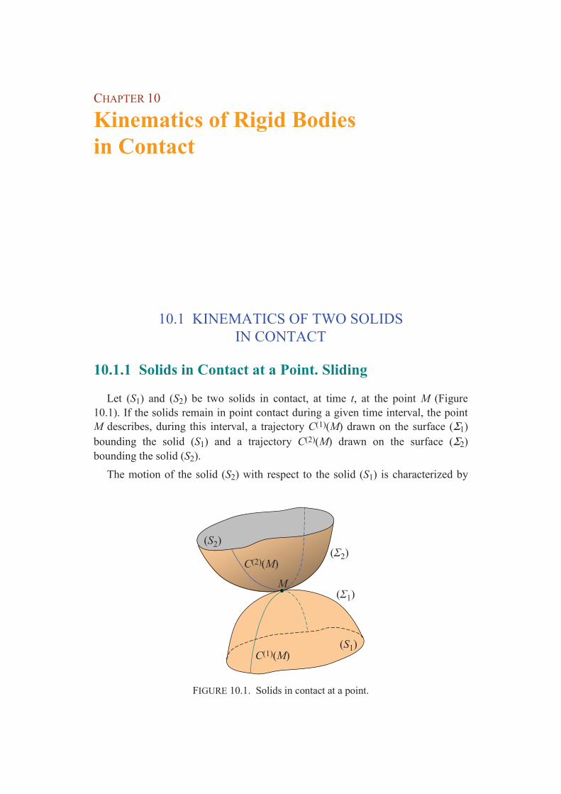
CHAPTER 10
Kinematics of Rigid Bodies in Contact
10.1 KINEMATICS OF TWO SOLIDS
IN CONTACT
10.1.1 Solids in Contact at a Point. Sliding
Let (S1) and (S2) be two solids in contact, at time t, at the point M (Figure
10.1). If the solids remain in point contact during a given time interval, the point
M describes, during this interval, a trajectory C(1)(M) drawn on the surface (Σ1)
bounding the solid (S1) and a trajectory C(2)(M) drawn on the surface (Σ2)
bounding the solid (S2).
The motion of the solid (S2) with respect to the solid (S1) is characterized by
FIGURE 10.1. Solids in contact at a point.
M
(S2)
(S1)
(1)
(2) C(2)(M)
C(1)(M)

138 Chapter 10 Kinematics of Rigid Bodies
the kinematic torsor ( ) 12 of resultant
( )12ω
which is the instantaneous rotation
vector of the motion. The point M being in motion relatively to the solids (S1) and
(S2), we obtain by analogy with Relation (9.100):
( ) ( ) ( )
1 2 12( , ) ( , ) MM t M t= +
, (10.1)
where the vectors ( )1 ( , )M t
and ( )2 ( , )M t
are the velocity vectors of the point
of contact M respectively with respect to the solid (S1) and with respect to the
solid (S2).
The moment at the point M of the kinematic torsor ( ) 12 introduced in the
preceding expression is called the velocity vector of sliding of the solid (S2) on the
solid (S1) at the point of contact M at time t. Hence:
( ) ( ) 1 12 2( , ) Mg M t =
. (10.2)
From (10.1), we have:
( ) ( ) ( )
1 1 22( , ) ( , ) ( , )g M t M t M t= −
. (10.3)
This relation shows that the sliding velocity vector is a direction of the plane of
direction vectors ( )1 ( , )M t
and ( )2 ( , ) ,M t
plane which is in coincidence with
the plane (T) tangent at M to the two surfaces (Σ1) and (Σ2) (Figure 10.2).
If the sliding velocity vector is not null, it is said that the solid (S2) slides on the
solid (S1) at the point M and at time t. On the contrary if this vector is null, it is
said that the solid (S2) does not slide on the solid (S1) at the point M and at time t.
10.1.2 Spinning and Rolling
When the two solids (S1) and (S2) are tangent at the point M it is usual to
resolve the rotation vector( )12ω
into the sum of two vectors of rotation:
FIGURE 10.2. Sliding, rolling and spinning.
(S1)
(S2)
M
( )
12 nω
( )
12 tω
( )12ω
( )12 ( , )g M t
tangent plane

10.1 Kinematics of Two Solids in Contact 139
— a vector ( )12 tω
of direction contained in the plane (T) tangent to (Σ1) and to
(Σ2);
— a vector ( )12 nω
of direction orthogonal to the plane (T) thus to the directions ( )1 ( , )M t
and ( )2 ( , )M t
.
Hence: ( ) ( ) ( )
1 1 12 2 2t nω ω ω= +
. (10.4)
These vectors are called rolling rotation vector ( )12 tω
and spinning rotation vector( )12 nω
. If n
is the unit direction vector of the normal at M to the tangent plane:
( ) ( )
( ) ( )
1 2
1 2
( , ) ( , )
( , ) ( , )
M t M tn
M t M t
∧=
∧
, (10.5)
we have:
( ) ( )( )( ) ( )( )
1 12 2
1 12 2
,
.
t
n
n n
n n
ω ω
ω ω
= × ×
= ⋅
(10.6)
If the rotation vector of rolling (or/and of spinning) is not null, it is said that the
solid (S2) rolls (or/and spins) on the solid (S1), at point M at time t. In contrast if
this vector is null, it is said that the solid (S2) does not roll (or/and does not spin).
10.1.3 Conclusions
If two solids (S2) and (S1) are in contact at the point M at time t, the motion of
(S2) with respect to (S1) is characterized by the elements of reduction at the point
M of the kinematic torsor ( ) 12 :
( ) ( )
( ) ( )
( ) ( )
1 12 2
1 12 2
2 1
, instantaneous rotation vector;
( , ) , velocity vector of at in the motion of on .
M g
R
M t sliding MS S
ω = =
(10.7)
The rotation vector is then resolved into two vectors: ( )12 tω
: rotation vector of rolling, of direction contained in the plane tangent at
the point M to the solids (S1) and (S2);
( )12 nω
: rotation vector of spinning, of direction orthogonal to the plane tangent
at the point M.
The nullity or not of these vectors characterizes then the type of motion of the
solid (S2) with respect to the solid (S1) at the point M, in accordance with Table
10.1.

140 Chapter 10 Kinematics of Rigid Bodies
TABLE 10.1 Sliding, rolling and spinning at a point of contact between two solids (S1) and
(S2).
If at a given time
( )12 tω
rolling
( )12 nω
spinning
( ) 12M
sliding
it is said that
0
0
0
(S2) rolls, spins and slides relatively to (S1).
0
0
= 0
(S2) rolls and spins without sliding.
0
= 0
= 0
(S2) rolls without sliding, nor spinning.
= 0
0
= 0
(S2) spins without sliding, nor rolling.
= 0
= 0
0
(S2) slides without rolling, nor spinning.
= 0
0
0
(S2) spins and slides without rolling.
0
= 0
0
(S2) rolls and slides without spinning.
10.1.4 Solids in Contact in Several Points
The preceding considerations can be applied in every point of contact, in the
case where the two solids are in contact in several points. In particular:
— If two solids (S1) and (S2) are in contact in two points and if the sliding
velocity vector is null in these two points, the rotation vector ( )12ω
is direction
vector of the line passing through these two points.
— If two solids (S1) and (S2) are in contact in more than two points and if the
sliding is null in all these points, they are necessarily aligned.
10.2 TRANSMISSION OF A MOTION
OF ROTATION
10.2.1 General Elements
Two solids (S1) and (S2) have rotation motions of respective axes ( )1 1,O k
and
( )2 2,O k
attached to a reference system (T). The problem of the transmission of
the rotation motions consists in finding mechanisms which allow to transform a
rotation motion of (S1) with respect to the support (T) into a rotation motion of
(S2) with respect to the support and such as if the motion of (S1) is uniform, the
10.2 Transmission of a Motion of Rotation 141
motion of (S2) is uniform also.
The motion of the solid (S1) with respect to the support (T) is characterized by
the kinematic torsor ( ) 1T of resultant:
( )1 1 1T kω ω=
. (10.8)
The motion of the solid (S2) with respect to the support (T) is characterized by
the kinematic torsor ( ) 2T of resultant:
( )2 2 2T kω ω=
. (10.9)
The motion of (S2) with respect to (S1) is thus characterized by the kinematic
torsor ( ) 1
2 such as:
( ) ( ) ( ) 1 2 2 1
T T= − . (10.10)
The instantaneous rotation vector of the motion of (S2) with respect to (S1) is:
( )
12 2 2 1 1k kω ω ω= −
. (10.11)
The axes ( )1 1,O k
and ( )2 2,O k
being the axes of rotation attached to the support
(T), the vector( )12ω
is a vector independent of time relatively to a basis of the refe-
rence (T).
10.2.2 Transmission by Friction
In the case of the transmission of rotation motions by friction, the transmission
is obtained through a direct contact between the two solids (S1) and (S2), without
sliding at the points of contact. It results from Section 10.1.4 that the solids must
be in contact through a straight line, which is the instantaneous rotation axis of the
motion of (S2) with respect to (S1) and hence ( )12ω
is direction vector. It is shown
that this axis () is fixed in the reference (T). The surfaces coming in contact are
the surfaces generated by the rotation of () about the axis ( )1 1,O k
for the solid
(S1) and by the rotation of () about the axis ( )2 2,O k
for the solid (S2). These
surfaces of contact which are the axoidal surfaces are thus revolution surfaces
They are right circular cylinders if the axes ( )1 1,O k
and ( )2 2,O k
are parallel,
right circular cones if the axes intersect, revolution hyperboloid if they are not in
the same plane.
At a point M of contact, Expression (10.10) leads to:
( ) ( ) ( ) ( ) 1 12 2 2 1( , ) T T
M M Mg M t = = −
. (10.12)
The condition of non sliding at the point M is thus written as:
( ) ( ) 2 1 0T TM M− =
. (10.13)
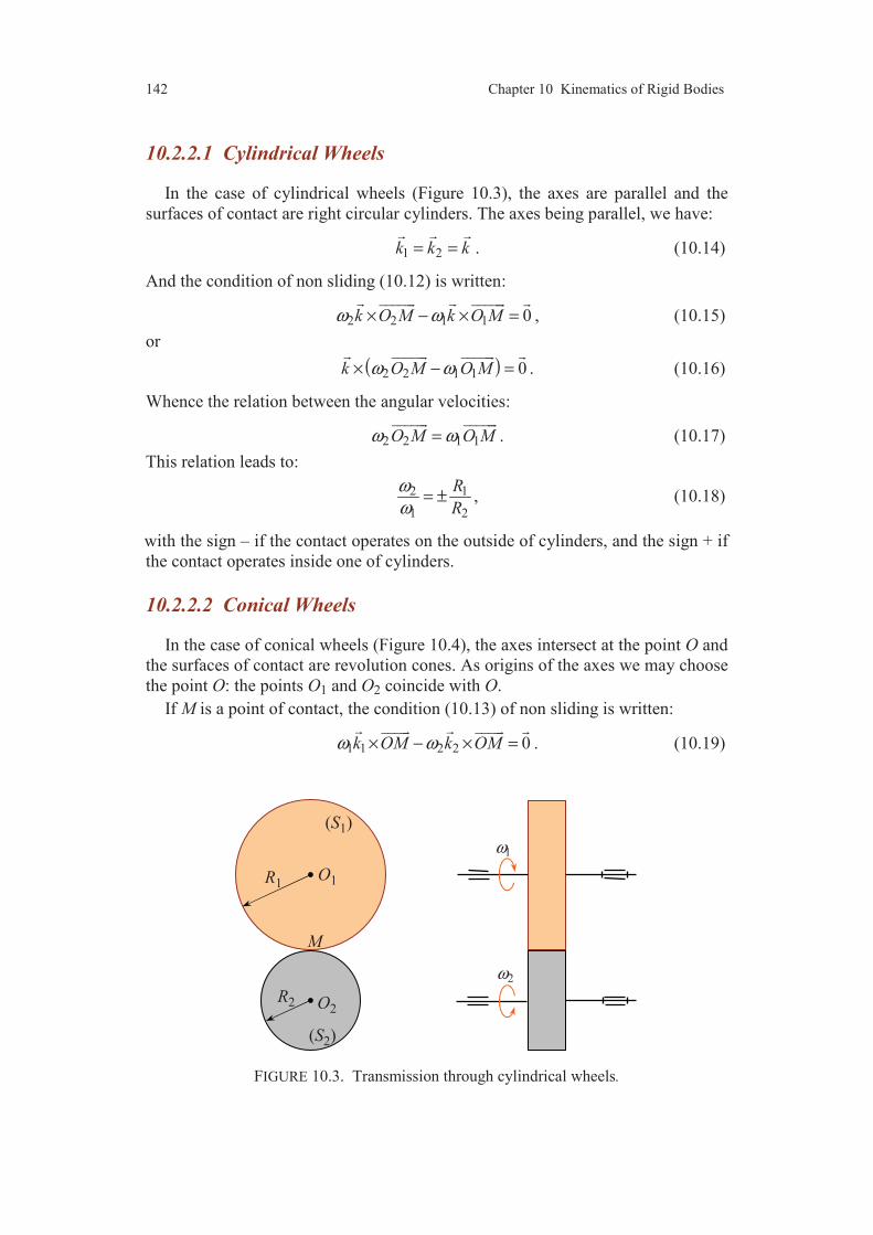
142 Chapter 10 Kinematics of Rigid Bodies
10.2.2.1 Cylindrical Wheels
In the case of cylindrical wheels (Figure 10.3), the axes are parallel and the
surfaces of contact are right circular cylinders. The axes being parallel, we have:
1 2k k k= =
. (10.14)
And the condition of non sliding (10.12) is written:
2 2 1 1 0k O M k O Mω ω× − × =
, (10.15)
or
( )2 2 1 1 0k O M O Mω ω× − =
. (10.16)
Whence the relation between the angular velocities:
2 2 1 1O M O Mω ω=
. (10.17)
This relation leads to:
2 1
1 2
R
R
ωω
= ± , (10.18)
with the sign – if the contact operates on the outside of cylinders, and the sign + if
the contact operates inside one of cylinders.
10.2.2.2 Conical Wheels
In the case of conical wheels (Figure 10.4), the axes intersect at the point O and
the surfaces of contact are revolution cones. As origins of the axes we may choose
the point O: the points O1 and O2 coincide with O.
If M is a point of contact, the condition (10.13) of non sliding is written:
1 1 2 2 0k OM k OMω ω× − × =
. (10.19)
FIGURE 10.3. Transmission through cylindrical wheels.
M
O1
O2
R1
R2
(S1)
(S2)
1ω
2ω
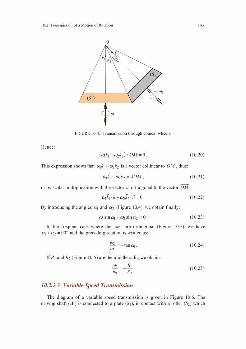
10.2 Transmission of a Motion of Rotation 143
FIGURE 10.4. Transmission through conical wheels.
Hence:
( )1 1 2 2 0k k OMω ω− × =
. (10.20)
This expression shows that 1 1 2 2k kω ω−
is a vector collinear to OM
, thus:
1 1 2 2k k OMω ω λ− =
, (10.21)
or by scalar multiplication with the vector u
orthogonal to the vector OM
:
1 1 2 2 0k u k uω ω− =⋅ ⋅
. (10.22)
By introducing the angles 1α and 2α (Figure 10.4), we obtain finally:
1 1 2 2sin sin 0ω α ω α+ = . (10.23)
In the frequent case where the axes are orthogonal (Figure 10.5), we have
1 2 90α α+ = ° and the preceding relation is written as:
21
1
tanω
αω
= − . (10.24)
If R1 and R2 (Figure 10.5) are the middle radii, we obtain:
2 1
1 2
R
R
ωω
= − . (10.25)
10.2.2.3 Variable Speed Transmission
The diagram of a variable speed transmission is given in Figure 10.6. The
driving shaft (∆1) is connected to a plate (S1), in contact with a roller (S2) which
O
1ω
2ω
(S1)
(S2)
1k 2k
12

144 Chapter 10 Kinematics of Rigid Bodies
FIGURE 10.5. Transmission through conical wheels with orthogonal axes.
can move along a radius of the plate. The angular velocity of the output is that of
the roller axis.
If x is the distance from the point of contact to the centre of the plate and if r is
the radius of the roller, we obtain without difficulty the relation:
2 1x
rω ω= − . (10.26)
The translation of the roller thus makes it possible to vary 2ω for a given 1ωangular velocity.
FIGURE 10.6. Variable speed transmission.
O
1ω
2ω
12
2R2
2R1
1ω
2ω
(S2)
(S1)
r
translation
x
(1)
M
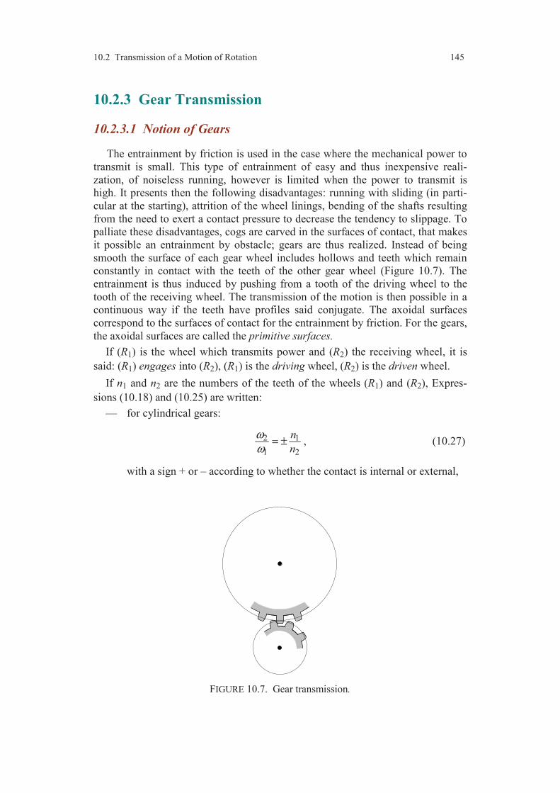
10.2 Transmission of a Motion of Rotation 145
10.2.3 Gear Transmission
10.2.3.1 Notion of Gears
The entrainment by friction is used in the case where the mechanical power to
transmit is small. This type of entrainment of easy and thus inexpensive reali-
zation, of noiseless running, however is limited when the power to transmit is
high. It presents then the following disadvantages: running with sliding (in parti-
cular at the starting), attrition of the wheel linings, bending of the shafts resulting
from the need to exert a contact pressure to decrease the tendency to slippage. To
palliate these disadvantages, cogs are carved in the surfaces of contact, that makes
it possible an entrainment by obstacle; gears are thus realized. Instead of being
smooth the surface of each gear wheel includes hollows and teeth which remain
constantly in contact with the teeth of the other gear wheel (Figure 10.7). The
entrainment is thus induced by pushing from a tooth of the driving wheel to the
tooth of the receiving wheel. The transmission of the motion is then possible in a
continuous way if the teeth have profiles said conjugate. The axoidal surfaces
correspond to the surfaces of contact for the entrainment by friction. For the gears,
the axoidal surfaces are called the primitive surfaces.
If (R1) is the wheel which transmits power and (R2) the receiving wheel, it is
said: (R1) engages into (R2), (R1) is the driving wheel, (R2) is the driven wheel.
If n1 and n2 are the numbers of the teeth of the wheels (R1) and (R2), Expres-
sions (10.18) and (10.25) are written:
— for cylindrical gears:
2 1
1 2
n
n
ωω
= ± , (10.27)
with a sign + or – according to whether the contact is internal or external,
FIGURE 10.7. Gear transmission.

146 Chapter 10 Kinematics of Rigid Bodies
— for conical gears with orthogonal axes:
2 1
1 2
n
n
ωω
= − . (10.28)
10.2.3.2 Gear Train
1. Gear train ratio A gear train is symbolized in Figure 10.8. The axes (∆1), (∆2), ... (∆p) of the
different wheels are fixed relatively to a support (T). Each intermediate axis (∆2),
(∆3), ... (∆p – 1) comprises a driving wheel (Ri) and a driven wheel ( iR′ ). The wheel
(R1) is a driving wheel and the wheel ( pR′ ) is a driven wheel. The gears are either
cylindrical, or conical.
It is found without difficulty that:
1 2 1
1 2 3
. . .
. . .
p p
p
n n n
n n n
ω
ω−
= ±′ ′ ′
, (10.29)
with the sign + or – according to the number of external contacts and according to
the number of conical gears. The quantity 1
pr
ω
ω= is called the ratio of the shear
train.
2. Epicyclic Trains The epicyclic trains are gear trains such as those described previously, but the
axes of which are connected to a frame (B) which is itself animated of a rotation
motion of angular velocity Ω about an axis (∆) attached to the reference (T). The
epicyclic train is schematized in Figure 10.9.
If r is the ratio of the gear train, we have:
1
pr
ω
ω= , (10.30)
where pω and 1ω are the angular velocities of the last driven wheel and the first
driving wheel relatively to the frame (B). Let Ωp and Ω1 be the angular velocities
FIGURE 10.8. Gear train.
1( )R
2( )R
3( )R
2( )R′
3( )R′ 4( )R′
1( )∆
2( )∆
3( )∆
4( )∆

10.2 Transmission of a Motion of Rotation 147
FIGURE 10.9. Epyciclic train.
relatively to the reference (T). The law (10.11) of the composition of the rotation
vectors leads, in the case where the axes (∆1), (∆p) and (∆) are parallel, to the
relations:
1 1, .p pω Ω Ω ω Ω Ω= − = −
Whence the expression of the ratio of the gear train:
1
pr
Ω Ω
Ω Ω
−=
−. (10.31)
This relation is called Willis formula.
3. Application to the case of car differential
Along a straight line the two wheels of a car turn at the same angular velocity
of rotation. When cornering, the distance covered by the external wheel is larger
than that covered by the internal wheel. It results from it that the external wheel
must turn more quickly than the internal wheel. This process is obtained using a
differential, of which the general diagram is given in Figure 10.10. A pinion asso-
ciated to the output shaft of the gear box makes turn a toothed wheel connected to
a cage. On the cage a planet (S) is assembled which gears with two driving wheels
(R1) and (R2). The ratio of the gear train (from the wheel (R1) to the wheel (R2)) is
1r = − , and the Willis formula is written:
22 1
1
1 or 2Ω Ω
Ω Ω ΩΩ Ω
−= − + =
−, (10.32)
where Ω is the angular velocity of the rotation of the cage.
When cornering, the internal wheel (the wheel (R1) for example) can turn with
a velocity lower than that of the external wheel. Along a straight line, the velo-
cities are the same: 2 1 2Ω Ω Ω= = .
1( )∆
2( )∆ 3( )∆
( )∆
(B)
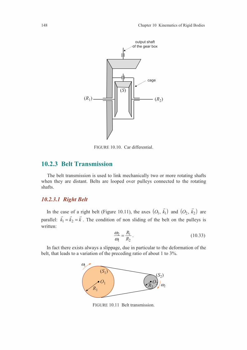
148 Chapter 10 Kinematics of Rigid Bodies
FIGURE 10.10. Car differential.
10.2.3 Belt Transmission
The belt transmission is used to link mechanically two or more rotating shafts
when they are distant. Belts are looped over pulleys connected to the rotating
shafts.
10.2.3.1 Right Belt
In the case of a right belt (Figure 10.11), the axes ( )1 1, O k
and ( )2 2, O k
are
parallel: 1 2k k k= =
. The condition of non sliding of the belt on the pulleys is
written:
2 1
1 2
R
R
ωω
= . (10.33)
In fact there exists always a slippage, due in particular to the deformation of the
belt, that leads to a variation of the preceding ratio of about 1 to 3%.
FIGURE 10.11 Belt transmission.
(R2) (R1)
(S)
cage
output shaft
of the gear box
O1 O2
R1
R2
(S1) (S2)
1ω
2ω

10.2 Transmission of a Motion of Rotation 149
FIGURE 10.12. Transmission with crossed belt.
10.2.3.2 Crossed Belt
In the case of a crossed belt (Figure 10.12) the angular velocities of rotation are
opposite:
2 1
1 2
R
R
ωω
= − . (10.34)
10.2.3.3 Set of Belts and Pulleys
In the case of a set of belts and pulleys (Figure 10.13), each intermediate axis
comprises a driving pulley (Si) of radius Ri and a driven pulley ( iS′ ) of radius iR′ . If the system comprises p axes, it is established without difficulty that:
1 2 1
1 2 3
. . .
. . .
p p
p
R R R
R R R
ω
ω−
= ±′ ′ ′
, (10.35)
with the sign + if the number of crossed belts is even, and the sign – if this
number is odd.
Note. To eliminate the slippage of the belts on the pulleys, the pulleys are repla-
ced by toothed wheels and the belts by chains. For example, Relation (10.33) is
then replaced by:
2 1
1 2
n
n
ωω
= , (10.36)
where n1 and n2 are respectively the number of the teeth of the wheels (1) and (2).
FIGURE 10.13. Set of belts and pulleys.
O1 O2
R1R2
(S1) (S2)
1ω
2ω
(S1)
1ω2ω
3ω
(S2)
2( )S ′
3( )S ′
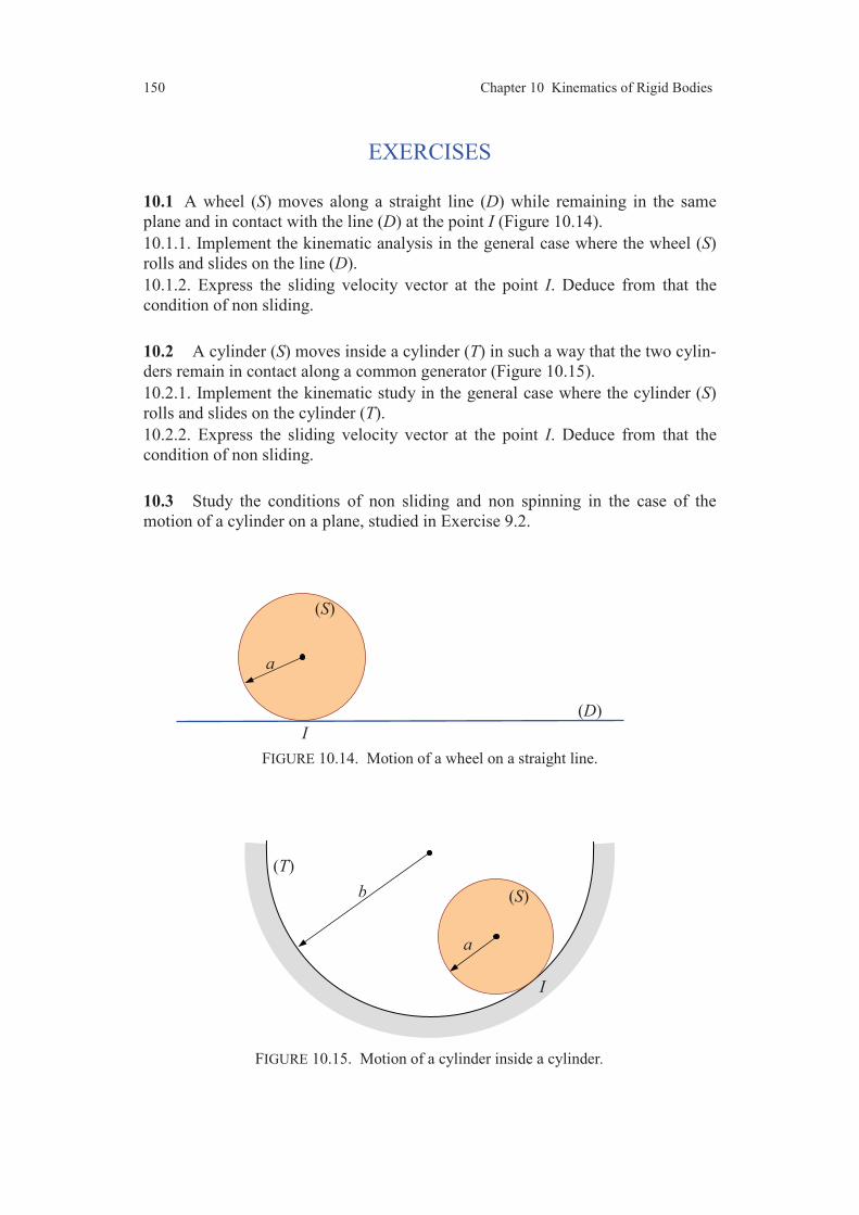
150 Chapter 10 Kinematics of Rigid Bodies
EXERCISES
10.1 A wheel (S) moves along a straight line (D) while remaining in the same
plane and in contact with the line (D) at the point I (Figure 10.14).
10.1.1. Implement the kinematic analysis in the general case where the wheel (S)
rolls and slides on the line (D).
10.1.2. Express the sliding velocity vector at the point I. Deduce from that the
condition of non sliding.
10.2 A cylinder (S) moves inside a cylinder (T) in such a way that the two cylin-
ders remain in contact along a common generator (Figure 10.15).
10.2.1. Implement the kinematic study in the general case where the cylinder (S)
rolls and slides on the cylinder (T).
10.2.2. Express the sliding velocity vector at the point I. Deduce from that the
condition of non sliding.
10.3 Study the conditions of non sliding and non spinning in the case of the
motion of a cylinder on a plane, studied in Exercise 9.2.
FIGURE 10.14. Motion of a wheel on a straight line.
FIGURE 10.15. Motion of a cylinder inside a cylinder.
I
a
(S)
(D)
a
(S)
I
b
(T)

Comments 151
COMMENTS
The kinematics of rigid bodies in contact is first implemented in the
usual way by using the concepts of the kinematics of solids considered in
the preceding chapter. Having determined the kinematic torsor relatively to
the motion of the two bodies in contact, its moment at a point of contact
allows us to derive the sliding velocity vector at this point of contact and
thus to analyze the conditions of non sliding. The instantaneous rotation
vector (resultant of the kinematic torsor) allows us then to analyze the
conditions of spinning and rolling.


Part III
The Mechanical Actions
The equilibrium or the motion of a solid of a set of solids results from
the mechanical actions which are exerted. These actions will be first
considered without being concerned with the physical phenomena by
which they are induced, and they will then be classified as force,
couple and arbitrary action. The actions of gravitation and the actions
of gravity will be studied in a particular chapter. Next, a chapter will
be devoted to the actions induced by connections, of which the
concept is at the basis of the technological design of the mechanical
systems. Lastly, the study of some problems of static equilibrium of
rigid bodies will allow us to understand the structuring of the
mechanical actions exerted on a solid or a set of solids.


CHAPTER 11
General Elements on the Mechanical Actions
11.1 CONCEPTS RELATIVE TO
THE MECHANICAL ACTIONS
11.1.1 Notion of Mechanical Action
The mechanical processes result from mechanical actions of which we have a
usual notion:
— an object, left to itself, falls: the Earth attracts the object;
— the same object, placed on a table, does not fall any more: the table exerts
on the object an action which prevents from falling;
— a child who kneads modelling clay exerts an action which deforms the
paste;
— the cyclist exerts on the pedals an action which produces the displacement
of the bicycle;
— the brake exerts an action which opposes to this displacement;
— etc.
Thus, in a general way, a mechanical action is a process which maintains an
equilibrium, causes a deformation, produces a motion or opposes to a motion.
11.1.2 Representation of a Mechanical Action
If the notion of mechanical action is usual, it is not in fact directly accessible
by measurement. We have knowledge of it only by its consequences: presence or
absence of equilibrium, measure of displacements, measure of deformations,
derivation of laws of motions, etc. Thus, to translate by equations the various

Chapter 11 General Elements on the Mechanical Actions 156
mechanical phenomena, we are brought to state the following axiom:
Any mechanical action which is exerted on a material set may be represented
by a torsor associated to this set.
We understand by material set either a rigid body, or a set of rigid bodies.
11.1.3 Classification of the Mechanical Actions
To each type of torsor corresponds a type of mechanical action whose the
properties are immediate consequences of the results established in Chapter 5.
11.1.3.1 Force
We say that an exerted mechanical action is a force, if and only if the torsor
representing the mechanical action is a slider.
It results from the properties derived in Section 5.2.1, that a force is character-
rized by:
— the resultant of the slider associated to the force, generally called by lan-
guage contraction: the resultant of the force (the norm of the resultant of the force
called intensity or magnitude of the force is expressed in newtons: N);
— the axis of null moments (determined by only one point when the resultant
is known), called support of the force or line of action.
If the mechanical action exerted on the set (D) is a force, it will be possible
symbolically to represent it by making appear the support (∆) of the force and a
bipoint (A, B) of which the image in 3 is the resultant of the force: R
(Figure
11.1a). If we are in the case studied in 5.3.3 of Chapter 5, the force has a measure
centre H defined by (5.69) or (5.72); and we shall take for the point A the measure
centre (Figure 11.1b).
Lastly, let us note that a force tends to move the set, on which it is exerted,
along the direction defined by the resultant, therefore parallel to the support of the
force.
11.1.3.2 Couple
We say that a mechanical action is a couple (couple-action), if and only if the
torsor which represents this action is a couple-torsor.
It results from the properties established in Section 5.2.2 that a couple is cha-
racterized by its moment-vector, independent of the point considered, and of
which the magnitude is expressed in N m. This moment-vector is sometimes
called couple. Let us note however it is necessary to distinguish the couple-
action, from the couple-torsor and from its moment-vector.
Furthermore, it results from Section 5.2.2 that a couple is equivalent to a
couple of two forces of opposite resultants, hence of parallel supports. There
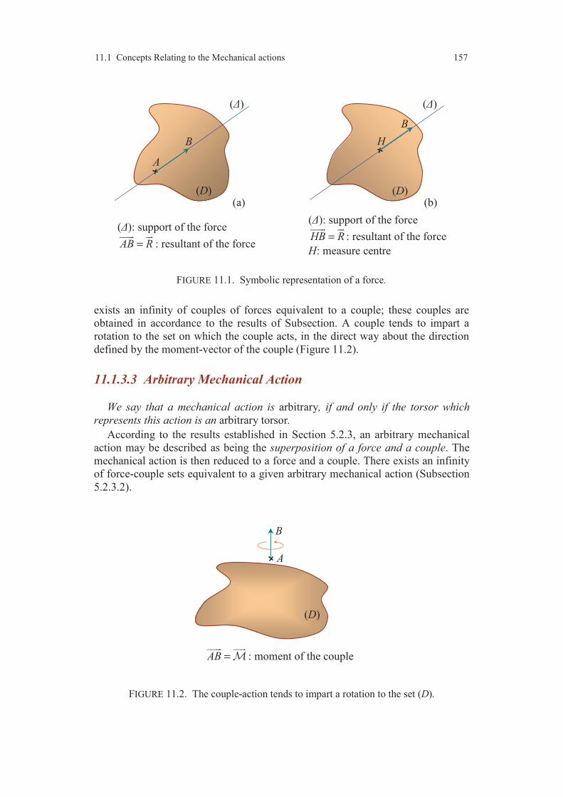
11.1 Concepts Relating to the Mechanical actions 157
FIGURE 11.1. Symbolic representation of a force.
exists an infinity of couples of forces equivalent to a couple; these couples are
obtained in accordance to the results of Subsection. A couple tends to impart a
rotation to the set on which the couple acts, in the direct way about the direction
defined by the moment-vector of the couple (Figure 11.2).
11.1.3.3 Arbitrary Mechanical Action
We say that a mechanical action is arbitrary, if and only if the torsor which
represents this action is an arbitrary torsor.
According to the results established in Section 5.2.3, an arbitrary mechanical
action may be described as being the superposition of a force and a couple. The
mechanical action is then reduced to a force and a couple. There exists an infinity
of force-couple sets equivalent to a given arbitrary mechanical action (Subsection
5.2.3.2).
FIGURE 11.2. The couple-action tends to impart a rotation to the set (D).
A
()
B
(D)
(): support of the force
AB R=
: resultant of the force
(): support of the force
HB R=
: resultant of the force
H: measure centre
(a)
H
()
B
(D) (b)
A
B
(D)
AB =
: moment of the couple

Chapter 11 General Elements on the Mechanical Actions 158
11.1.4 Mechanical Actions Exerting between Material Sets
Let (D1) and (D2) be two material sets. The mechanical actions exerted by (D1)
on (D2) are represented by the torsor which we shall denote by:
1 2D D→ . (11.1)
In the same way, the mechanical actions exerted by (D2) on (D1) are represented
by the torsor denoted by:
2 1D D→ . (11.2)
1. Superposition of the generators of mechanical actions
If the set (D1) is constituted of the union of two disjoint sets ( )1D′ and ( )1D′′ , we
shall write:
1 2 1 1 2 1 2 1 2( )D D D D D D D D D′ ′′ ′ ′′→ = ∪ → = → + → . (11.3)
2. Superposition of the receivers of mechanical actions
If the set (D2) is constituted of the union of two disjoint sets ( )2D′ and ( )2D′′ ,
we shall write in the same way:
1 2 1 2 2 1 2 1 2( )D D D D D D D D D′ ′′ ′ ′′→ = → ∪ = → + → . (11.4)
Relations (11.3) and (11.4) combine and extend to the cases where the sets
considered are the unions of an arbitrary finite number of disjoint sets.
11.1.5 External Mechanical Actions Exerting on a Material Set
The Universe which shall be denoted by (U) is the material set of all the phy-
sical systems which are more or less distant: chair, table, house, city, country,
Earth, planets, Sun, stars, etc. Being given a set (D), we call exterior of the set
(D), which we shall denote by ( )D , the complement of (D) in the Universe; that is
saying all that in the Universe is not (D):
( ) ( ) ( ), D D U D D∪ = ∩ = ∅ . (11.5)
We call mechanical actions exerting on the set (D), or actions external to (D),
the set of mechanical actions exerted on (D) by the exterior of (D). These actions
are represented by the torsor:
D D→ . (11.6)
The exterior of (D) is constituted of disjoint subsets: ( ) ( ) ( ) 1 2, , . . . , nD D D .
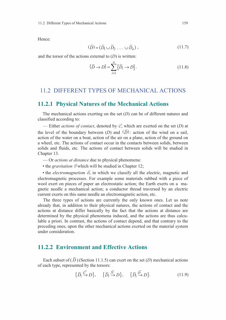
11.2 Different Types of Mechanical Actions 159
Hence:
( ) ( )1 2 . . . nD D D D= ∪ ∪ , (11.7)
and the torsor of the actions external to (D) is written:
1
n
i
i
D D D D
=
→ = → . (11.8)
11.2 DIFFERENT TYPES OF MECHANICAL ACTIONS
11.2.1 Physical Natures of the Mechanical Actions
The mechanical actions exerting on the set (D) can be of different natures and
classified according to:
— Either actions of contact, denoted by , which are exerted on the set (D) at
the level of the boundary between (D) and ( )D : action of the wind on a sail,
action of the water on a boat, action of the air on a plane, action of the ground on
a wheel, etc. The actions of contact occur in the contacts between solids, between
solids and fluids, etc. The actions of contact between solids will be studied in
Chapter 13.
— Or actions at distance due to physical phenomena:
• the gravitation which will be studied in Chapter 12;
• the electromagnetism , in which we classify all the electric, magnetic and
electromagnetic processes. For example some materials rubbed with a piece of
wool exert on pieces of paper an electrostatic action; the Earth exerts on a ma-
gnetic needle a mechanical action; a conductor thread traversed by an electric
current exerts on this same needle an electromagnetic action, etc.
The three types of actions are currently the only known ones. Let us note
already that, in addition to their physical natures, the actions of contact and the
actions at distance differ basically by the fact that the actions at distance are
determined by the physical phenomena induced, and the actions are thus calcu-
lable a priori. In contrast, the actions of contact depend, and that contrary to the
preceding ones, upon the other mechanical actions exerted on the material system
under consideration.
11.2.2 Environment and Effective Actions
Each subset of ( D ) (Section 11.1.5) can exert on the set (D) mechanical actions
of each type, represented by the torsors:
, , .i i iD D D D D D→ → →
(11.9)

Chapter 11 General Elements on the Mechanical Actions 160
If the subset ( )iD exerts simultaneously the three types of actions, the actions
exerted by ( )iD on the set (D) are represented by the torsor:
,i ii iD D D DD D D D= + +→ →→ →
(11.10)
and the torsor (11.8) of the mechanical actions exerted on (D) is written:
1
n
ii i
i
D DD D D D D D
=
= + +→→ → → . (11.11)
In practice, by taking account of the expressions of the physical laws of the
actions at distance, it will be possible to neglect such or such action of such or
such set ( )iD of the exterior of the set (D) considered. For example, for a material
system in the vicinity of the Earth, the actions of gravitation exerted by the Earth
are preponderant compared to the gravitation exerted by the Moon, the planets,
the Sun. In the same way, the action of gravitation exerted on a magnetic needle
by a conductor thread crossed by an electric current can be neglected in front of
its electromagnetic action. Thus, Expression (11.11) of the torsor of the mecha-
nical actions exerted on the set (D) can be simplified, in accordance with the
problems considered, by taking into account only the preponderant mechanical
actions. We shall denote generally by ( ) D the torsor (11.11) simplified of the
preponderant actions exerted on the set (D). We shall write:
( ) ( ) j
j
D D= , (11.12)
where ( ) j D is the torsor which represents the preponderant action j.
11.3 POWER AND WORK
11.3.1 Definition of the Power
We call power developed, at time t, relatively to the reference (T), by the
action j acting on solid (S) and represented by the torsor ( ) j S , the scalar:
( ) ( ) ( ) ( ) T Tj j SP S S= ⋅ . (11.13)
If M is a point of the solid (S), the power is written, from (5.15):
( ) ( ) ( ) ( ) ( ) ( ) T T TM Mj j jS SP S R S S R= +⋅ ⋅
, (11.14)
or, by introducing the elements of reduction (9.18) and (9.19) of the kinematic
torsor at the point M:
( ) ( ) ( ) ( )( ) ( ) ( ),T T T
Mj j j SP S R S M t S ω= +⋅ ⋅
. (11.15)

11.3 Power and Work 161
11.3.2 Change of Reference System
Let (1) and (2) be two reference systems. The power developed relatively to
the reference (1) is: ( ) ( ) ( ) ( ) 1 1
j j SP S S= ⋅ , (11.16)
the power developed relatively to the reference (2) is:
( ) ( ) ( ) ( ) 2 2j j SP S S= ⋅ . (11.17)
From these two relations and from the law (9.39) of compositions of motions, we
derive the relation: ( ) ( ) ( ) ( ) ( ) ( ) 1 2 1
2j j jP S P S S= + ⋅ . (11.18)
11.3.3 Potential Energy
It happens that, having derived the developed power, we observe that the
power can be put in the form of a derivative with respect to time of a function
which depends only on the parameters of situation 1 2( , , . . . , )kq q q and eventually
on time. Hence:
( ) ( ) ( ) p 1 2
d ( , , . . . , , )d
T Tj kP S E q q q t
t= − . (11.19)
The function ( )pTE , thus defined except for an additive constant (independent of
the parameters qi and time t), is called potential energy of the solid (S) relatively
to the reference (T). It is thus said that the mechanical action exerted on (S) and
represented by the torsor ( ) j S admits a potential energy in the reference (T).
It should however be noted that this case is not general.
Example. Action exerted by a spring.
Let us consider a spring (R) (Figure 11.3) of negligible mass and of axis AA1
fixed in the reference (T). The experimental study shows that the mechanical
action exerted by the spring (R) on the solid (S) is a force of support AA1, repre-
sented by a slider R S→ of which the resultant is proportional to the
elongation (positive or negative) of A1A from the initial length l0 of the spring
when no action is exerted on the spring: the point A1 is then at A0. For a position
of the point A1, defined by 1AA l= , it is observed experimentally that:
— if 0l l> , the spring is stretched and it tends to draw back the point A1 at A0
by attracting A1 towards A0;
— if 0l l< , the spring is compressed and it tends to push back A1 towards A0.
By taking as axis Ax
the axis of the spring, the experimental results observed
are described while writing:

Chapter 11 General Elements on the Mechanical Actions 162
FIGURE 11.3. Spring of traction-compression.
( )
0 ,
0, point of the axis ,P
R R S k x l i
R S P Ax
→ = − −
→ = ∀
(11.20)
where k is a constant characteristic of the spring, called coefficient of rigidity or
stiffness of the spring, and x is the abscissa of the point A1 on the axis Ax
.
In the case of rectilinear translation motion of axis Ax
, the kinematic torsor
relative to the motion of the solid (S) with respect to reference (T) is written at the
point A1:
( ) ( )
( ) ( )1 1
0,
( , ) .
T TS S
T TA S
R
A t x i
ω = =
= =
(11.21)
By expressing in the present case Relation (11.13), we obtain:
( ) ( ) ( )
20 0
d dd d 2
T x kP R S k x l x lt t
→ = − − = − − . (11.22)
From this we deduce that the action exerted by the spring admits a potential ener-
gy in the reference (T) of the form:
( ) ( )2p 0 cte
2T kE x l= − + . (11.23)
11.3.4 Work
We call work in the reference (T), between the instants t1 and t2, of a mecha-
nical action represented by the torsor ( ) j S the integral:
(T)
A0
(S)
A1
A
11.3 Power and Work 163
( ) ( ) ( ) 2
1
1 2( , ) dt
T Tj
t
W t t P S t= . (11.24)
If the mechanical action admits a potential energy in the reference (T), the
work is written from (11.19):
( ) ( ) ( )1 2 p 1 p 2( , ) ( ) ( )T T TW t t E t E t= − . (11.25)
Work thus depends only upon the initial state and the final state of the solid.
11.3.5 Power and Work of a Force
11.3.5.1 Power
If the action exerting on the solid (S) is a force, the torsor ( ) j S which
represents this action is a slider, and Expression (11.15) is written at a point P of
the support of the force:
( ) ( ) ( ) ( ) ( ),T Tj jP S R S P t= ⋅
. (11.26)
If the position vector of the point P in the reference (T) does not depend expli-
citly on time, we have, by introducing the parameters qi of situation:
( )( )( )
1
d, d
kTT
ii
i
OPM t OP qt q
=
∂= =∂
, (11.27)
where O is a point fixed in reference (T). Expression (11.26) of the power is then
written:
( ) ( ) ( ) 1
kT
j j ii
i
OPP S R S qq
=
∂=∂
⋅
. (11.28)
Case where the force admits a potential energy
In the case where the force admits in the reference (T) a potential energy which
does not depend explicitly on time, Relation (11.19) is written:
( ) ( ) ( ) p 1 2
1
( , , . . . , )
kT T
j k ii
i
P S E q q q qq
=
∂= −∂ . (11.29)
By comparing Expressions (11.28) and (11.29), we obtain:
( ) ( ) ( )pT T
ji i i
OPR S E Uq q q
∂ ∂ ∂= − =∂ ∂ ∂
⋅
, (11.30)
setting: ( ) ( )
pT TU E C= − + ,
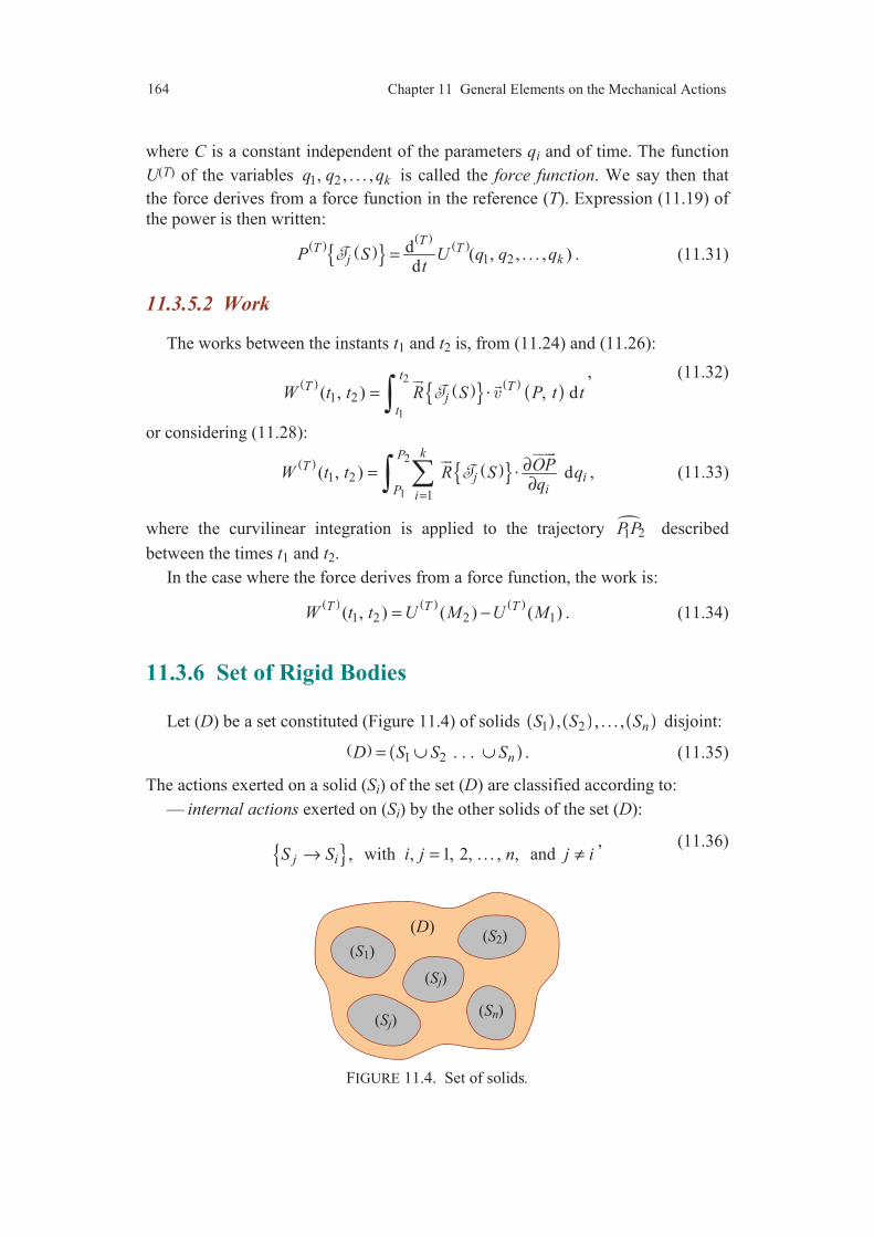
Chapter 11 General Elements on the Mechanical Actions 164
where C is a constant independent of the parameters qi and of time. The function
U(T) of the variables 1 2, , . . . , kq q q is called the force function. We say then that
the force derives from a force function in the reference (T). Expression (11.19) of
the power is then written:
( ) ( ) ( )
( ) 1 2
d ( , , . . . , )d
TT T
j kP S U q q qt
= . (11.31)
11.3.5.2 Work
The works between the instants t1 and t2 is, from (11.24) and (11.26):
( ) ( ) ( ) ( )
2
1
1 2( , ) , dt
T Tj
t
W t t R S P t t= ⋅
, (11.32)
or considering (11.28):
( ) ( ) 2
1
1 2
1
( , ) d
kPT
j iiP i
OPW t t R S qq
=
∂=∂
⋅
, (11.33)
where the curvilinear integration is applied to the trajectory 21P P described
between the times t1 and t2.
In the case where the force derives from a force function, the work is:
( ) ( ) ( )1 2 2 1( , ) ( ) ( )T T TW t t U M U M= − . (11.34)
11.3.6 Set of Rigid Bodies
Let (D) be a set constituted (Figure 11.4) of solids ( ) ( ) ( ) 1 2, , . . . , nS S S disjoint:
( ) ( )1 2 . . . nD S S S= ∪ ∪ . (11.35)
The actions exerted on a solid (Si) of the set (D) are classified according to:
— internal actions exerted on (Si) by the other solids of the set (D):
, with , 1, 2, . . . , , and j iS S i j n j i→ = ≠, (11.36)
FIGURE 11.4. Set of solids.
(S1)
(Sj)
(Sj)
(S2)
(Sn)
(D)

Exercises 165
— external actions exerted on (Si) by the exterior of (D):
iD S→ . (11.37)
The resultant mechanical action exerted on the solid (Si) is represented by the
torsor:
1
n
i i i j i
ji
S S D S S S
=≠
→ = → + → , (11.38)
external actions internal actions
and the power developed by the whole of the actions exerted on the solid (Si) is
written:
( ) ( ) ( ) 1
nT T T
i i i j i
ji
P S S P D S P S S
=≠
→ = → + → . (11.39)
We call power developed in the reference (T) on the set (D), the sum of the
powers developed on all the solids. Thus:
( ) ( ) ( ) ( )
1 1 1
n n nT T T
i j i
i i ji
P D P D S P S S
= = =≠
= → + → . (11.40)
The first term can be put in the form:
( ) ( ) ( )
11 1
n n nT T T
i i ii
i i
P D S P D S P D S=
= =
→ = → + →
∪ . (11.41)
Thus finally:
( ) ( ) ( ) ( ) 1 1
n nT T T
i j i
i ji
P D P D S P S S
= =≠
= → + → . (11.42)
set of the set of the
external actions internal actions
EXERCISES
11.1 In a preliminary design of the calculation of a frame, we have to consider
(Figure 11.5) the field of forces defined on the set of the points Mi reported in the
figure. The supports of the forces i corresponding to each point Mi are contained
in the plane Oxy. The figure shows the direction of the support of each force,
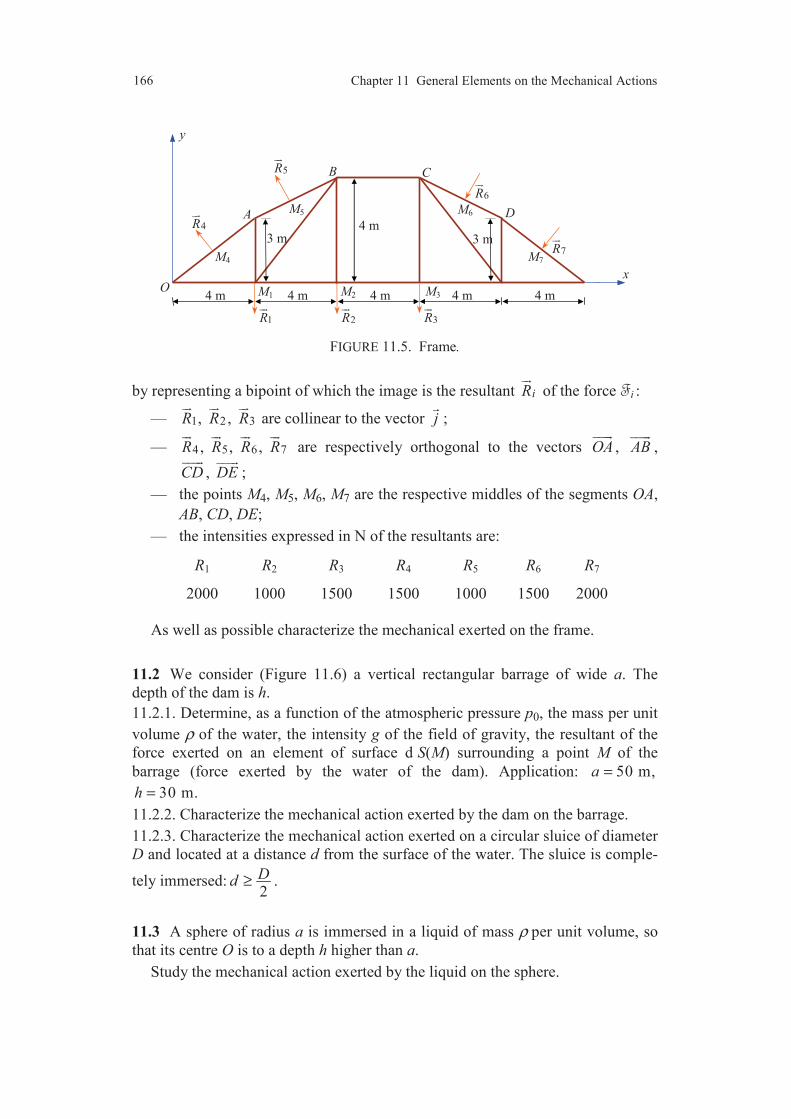
Chapter 11 General Elements on the Mechanical Actions 166
FIGURE 11.5. Frame.
by representing a bipoint of which the image is the resultant iR
of the force i :
— 1 2 3, , R R R
are collinear to the vector j
;
— 4 5 6 7, , , R R R R
are respectively orthogonal to the vectors OA
, AB
,
CD
, DE
;
— the points M4, M5, M6, M7 are the respective middles of the segments OA,
AB, CD, DE;
— the intensities expressed in N of the resultants are:
R1 R2 R3 R4 R5 R6 R7
2000 1000 1500 1500 1000 1500 2000
As well as possible characterize the mechanical exerted on the frame.
11.2 We consider (Figure 11.6) a vertical rectangular barrage of wide a. The
depth of the dam is h.
11.2.1. Determine, as a function of the atmospheric pressure p0, the mass per unit
volume ρ of the water, the intensity g of the field of gravity, the resultant of the
force exerted on an element of surface d S(M) surrounding a point M of the
barrage (force exerted by the water of the dam). Application: 50 m,a =
30 m.h =
11.2.2. Characterize the mechanical action exerted by the dam on the barrage.
11.2.3. Characterize the mechanical action exerted on a circular sluice of diameter
D and located at a distance d from the surface of the water. The sluice is comple-
tely immersed:2Dd ≥ .
11.3 A sphere of radius a is immersed in a liquid of mass ρ per unit volume, so
that its centre O is to a depth h higher than a.
Study the mechanical action exerted by the liquid on the sphere.
4 m 4 m 4 m 4 m 4 m
M4
M5 M6
M7
M1 M2 M3
4R
5R
6R
7R
y
O
A
B C
D
1R
2R
3R
x
4 m 3 m 3 m
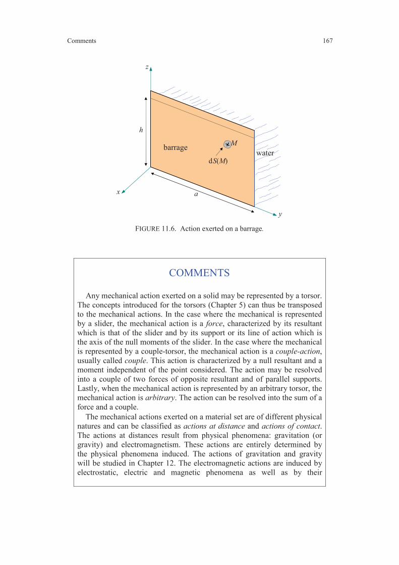
Comments 167
FIGURE 11.6. Action exerted on a barrage.
COMMENTS
Any mechanical action exerted on a solid may be represented by a torsor.
The concepts introduced for the torsors (Chapter 5) can thus be transposed
to the mechanical actions. In the case where the mechanical is represented
by a slider, the mechanical action is a force, characterized by its resultant
which is that of the slider and by its support or its line of action which is
the axis of the null moments of the slider. In the case where the mechanical
is represented by a couple-torsor, the mechanical action is a couple-action,
usually called couple. This action is characterized by a null resultant and a
moment independent of the point considered. The action may be resolved
into a couple of two forces of opposite resultant and of parallel supports.
Lastly, when the mechanical action is represented by an arbitrary torsor, the
mechanical action is arbitrary. The action can be resolved into the sum of a
force and a couple.
The mechanical actions exerted on a material set are of different physical
natures and can be classified as actions at distance and actions of contact.
The actions at distances result from physical phenomena: gravitation (or
gravity) and electromagnetism. These actions are entirely determined by
the physical phenomena induced. The actions of gravitation and gravity
will be studied in Chapter 12. The electromagnetic actions are induced by
electrostatic, electric and magnetic phenomena as well as by their
M
dS(M)
y
x
z
h
a
barrage water

Chapter 11 General Elements on the Mechanical Actions 168
couplings. The actions of contact are exerted on a system at the level of its
boundary. In contrast to the actions at distance, the actions of contact
depend on the other actions exerted on the material system. Their complete
characterization can then be obtained only as part of the resolution of the
problem of mechanics.
An important notion introduced is that of the power developed by a
mechanical action exerted on a moving solid. This power is expressed
simply as the product of the torsor which represents the mechanical by the
kinematic torsor relative to the motion of the solid. The power is an instan-
taneous quantity which expresses a state at every moment. The concept of
work which is deduced from it, by integration of the power with respect to
time, is less interesting.

CHAPTER 12
Gravitation. Gravity Mass Centre
12.1 PHENOMENON OF GRAVITATION
12.1.1 Law of Gravitation
The law of gravitation (or Newton’s law) introduces the concept of mass of a
material system, physical quantity which allows us to measure the quantity of
matter of the material system. The law of gravitation may be formulated in the
following way.
Let us consider two material elements of centres M and M', of respective
masses m and m'. Because of its presence, the material element of centre M' exerts
on the set of centre M a mechanical action (the torsor representing this mecha-
nical action will be denoted by M M′ → ). This action is a force of support
MM' and of resultant:
( )3
MMR KmmM M
MM
′′′ =→
′
, (12.1)
where K is the universal constant of gravitation:
K = 6,67 × 10⁻¹¹ m3 kg–1 s–2.
The law of gravitation is all the more verified as the material elements have
dimensions (Figure 12.1) which are low compared to the distance from M to .M ′All occurs then as if the masses of the material sets were respectively concen-
trated at the points M and .M ′ The points M and M ′ associated to their respective
masses m and m' are called material points.
It results from the statement of the law of gravitation that:
1. The torsor M M′ → which represents the action of gravitation exerted by
M ′ on M is a slider of elements of reduction:

170 Chapter 12 Gravitation. Gravity. Mass Centre
FIGURE 12.1. Material elements.
( )
3,
0, point of the line passing through and .P
MMR KmmM M
MM
P M MM M
′′′ =→
′
′′ = ∀→
(12.2)
2. The action of gravitation exerted by M on M' is a force opposite to the prece-
ding one, that is to say of the same support as the action exerted by M' on M, but
with an opposite resultant.
12.1.2 Gravitational Field
We call vector of the gravitational field at a point of the space, the resultant of
the action of gravitation exerted at this point on the unit mass.
The gravitation field induced by the material point (M', m') is then defined at
the point M by the vector:
( )3( )M
MMG M Km
MM′
′′=
′
, (12.3)
and the resultant of the action of gravitation is written:
( )MR m G MM M ′′ =→
. (12.4)
The magnitude of the gravitation field is expressed in N kg–1.
12.1.3 Action of Gravitation Induced by a Solid Sphere
Let us consider (Figure 12.2) a material point (M, m) located at a distance r of
the centre O of a solid sphere (S) of mass mS. An element of mass d ( )m M ′ sur-
rounding a point M' of the sphere exerts on M a force of resultant:
( )3
d d ( )MM
R Km m MM MMM
′′′ =→
′
, (12.5)
or
( )
3d ( )d ( )
MMR Km M V MM M
MMρ
′′ ′′ =→
′
, (12.6)
M(m)
M'(m')

12.1 Phenomenon of Gravitation 171
FIGURE 12.2. Action of gravitation exerted by a sphere.
where ( )Mρ ′ is the mass per unit volume of the sphere at the point M ′ and
d ( )V M ′ is the element of volume surrounding the point M'. The action of gravi-
tation exerted by the sphere on the point (M, m) is then represented by the torsor
associated to the field of sliders defined by (12.5) or (12.6). Thus, from (5.54) and
(5.55):
( ) ( )
( )
3( )d ( ),
d 0.
S
MS
MMR Km M V MS MMM
MM R M MS M
ρ′ ′ ′=→′
′= ∧ ′ =→→
(12.7)
The action of gravitation is thus a force of support passing through the point M.
In the case where the sphere is homogeneous by concentric layers, that is saying
for a sphere of which the mass per unit volume depends only on the distance R
from the centre of the sphere:
( ) ( )M Rρ ρ′ = , (12.8)
it is shown (Exercise 12.7) that the resultant of the action is expressed as follows:
3S
MOR KmmS M
OM=→
. (12.9)
The action of gravitation exerted by the sphere on the material point is thus a
force of support OM, identical to the action of gravitation which would be exerted
by a material point of mass equal to that of the sphere and placed at the centre of
the sphere.
The gravitational field induced at the point M by the sphere is then:
3( )S S
MOG M Km
OM=
. (12.10)
The expression of the field can be rewritten by introducing the unit direction
M
dm(M')
(S)
O
r
M ′

172 Chapter 12 Gravitation. Gravity. Mass Centre
vector ( )n M
of the line MO orientated from M towards O:
2( ) ( )S
SKm
G M n Mr
=
, (12.11)
where r is the distance from the point M to the centre of the sphere (Figure 12.2).
12.1.4 Action of Gravitation Induced by the Earth
In all the problem of engineering at the surface of the Earth or in its vicinity,
the gravitational actions of the other systems, in particular of the Moon and the
Sun, are negligible compared to the action of gravitation of the Earth. Further-
more, at first approximation, the simplifying assumption of an Earth spherical and
homogeneous by concentric layers is sufficient. It then follows from the results
derived in the preceding subsection that the action of gravitation exerted by the
Earth at the point M is a force of support passing though the point M and the
centre of the Earth, with the gravitational field:
TeTe
2( ) ( )
KmG M n M
r=
, (12.12)
where mTe is the mass of the earth, r is the distance from the point M to the centre
of the Earth and ( )n M
the unit direction vector of the line passing through the
point M and the centre of the Earth, orientated towards the centre of the Earth
(Figure 12.3).
If the point M is located on the surface of the Earth, the gravitational field is
written:
Te( ) ( )G M G n M=
, (12.13)
with
Te2
KmG
R= , (12.14)
FIGURE 12.3. Action of gravitation exerted by the Earth.
M
Earth
OTe
r
R
( )n M

12.2 Action of Gravity 173
where R is the radius of the Earth. If the point M is located at the altitude h, the
gravitational field induced by the Earth is written:
Te( ) ( ) ( )G M G h n M=
, (12.15)
with:
( )2
( )
1
GG hhR
=
+
. (12.16)
We observe that for an altitude much lower than the radius of the Earth, the
intensity G(h) of the gravitational field does not depend on h and coincides with
its value at the surface of the Earth. Moreover, at the scale of the technological
works the unit vector ( )n M
is independent of the point M:
( )n M n=
, (12.17)
where n
is the unit vector of the direction of the place of work to the centre of the
Earth. It results that the gravitational field is uniform at any point of the work:
Te point of the work ( ) .M G M G n∀ ≈
(12.18)
That is the model which we shall consider thereafter for any problem of me-
chanics relative to systems located at the vicinity of the Earth.
12.2 ACTION OF GRAVITY
12.2.1 Gravity Field Induced by the Earth
On the action of gravitation, exerted by the Earth on a material system placed
at its surface or at its vicinity, another mechanical action is superimposed due to
the rotation motion (Figure 12.4) of the Earth around its axis South-North. The
FIGURE 12.4. Action of gravity exerted by the Earth.
M
Earth
OTe
North
South
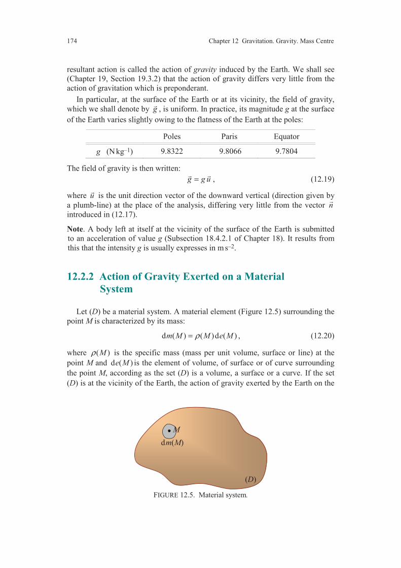
174 Chapter 12 Gravitation. Gravity. Mass Centre
resultant action is called the action of gravity induced by the Earth. We shall see
(Chapter 19, Section 19.3.2) that the action of gravity differs very little from the
action of gravitation which is preponderant.
In particular, at the surface of the Earth or at its vicinity, the field of gravity,
which we shall denote by g
, is uniform. In practice, its magnitude g at the surface
of the Earth varies slightly owing to the flatness of the Earth at the poles:
Poles Paris Equator
g (N kg–1) 9.8322 9.8066 9.7804
The field of gravity is then written:
g g u=
, (12.19)
where u
is the unit direction vector of the downward vertical (direction given by
a plumb-line) at the place of the analysis, differing very little from the vector n
introduced in (12.17).
Note. A body left at itself at the vicinity of the surface of the Earth is submitted
to an acceleration of value g (Subsection 18.4.2.1 of Chapter 18). It results from
this that the intensity g is usually expresses in m s–2.
12.2.2 Action of Gravity Exerted on a Material System
Let (D) be a material system. A material element (Figure 12.5) surrounding the
point M is characterized by its mass:
d ( ) ( )d ( )m M M e Mρ= , (12.20)
where ( )Mρ is the specific mass (mass per unit volume, surface or line) at the
point M and d ( )e M is the element of volume, of surface or of curve surrounding
the point M, according as the set (D) is a volume, a surface or a curve. If the set
(D) is at the vicinity of the Earth, the action of gravity exerted by the Earth on the
FIGURE 12.5. Material system.
dm(M)
M
(D)

12.2 Action of Gravity 175
element d ( )e M is a force of support ( ),M u
and of resultant:
d ( ) ( )d ( )R M g M m M=
, (12.21)
where ( )g M
is the field of gravity at the point M. For a material set located at the
vicinity of the Earth, the field of gravity is uniform and given by Expression
(12.19). The resultant is thus written as:
d ( ) d ( ) ( )d ( )R M u g m M u g M e Mρ= =
. (12.22)
The action of gravity exerted on the set (D) is thus represented by the torsor
associated to the field of sliders (or the field of forces) defined on the set (D) by
Relation (12.22). We are in the case of the field of sliders having parallel axes
independent of the point M (Section 5.3.3). From the results established in this
section, we deduce the following consequences.
The torsor ( ) e D which represents the action of gravity exerted by the Earth
on the set (D) located on its surface or at its vicinity:
1. has a measure centre G, called the mass centre of the set (D), defined by
one of the equivalent relations deduced from (5.69) and (5.72):
( )
1 d ( )D
OG OM m Mm
=
, (12.23)
or
( )d ( ) 0
D
GM m M =
, (12.24)
where m is the mass of the set (D) ;
2. is a slider of axis ( ),G u
and resultant:
( ) eR D mg u= , (12.25)
where u
is the unit direction vector of the downward vertical at the place of the
study.
The action of gravity exerted by the Earth on the set (D) is thus a force of
which the line of action passes through the mass centre of the set (D) and of which
the direction is given by the downward vertical. The magnitude of the force:
P mg= (12.26)
is called the weight of the set (D).
12.2.3 Power Developed by the Action of Gravity
Let (D) be a material set of mass m and of mass centre G, located on the
surface of the Earth or at its vicinity. The power developed by the action of
gravitation exerted on the set (D) is, from (11.26):

176 Chapter 12 Gravitation. Gravity. Mass Centre
FIGURE 12.6. Power developed by the action of gravity between two positions of the
mass centre of a material set.
( ) ( ) ( )e ( , )T TP D mg u G t= ⋅
. (12.27)
In a reference system (Oxyz) attached to the Earth and such as the axis Oz
is
upward vertical:
k u= −
, (12.28)
the position vector of the mass centre is written:
G G GOG x i y j z k= + +
, (12.29)
by introducing the Cartesian coordinates (xG, yG, zG) of the point G. The velocity
vector of the mass centre is:
( ) ( , )T
G G GG t x i y j z k= + +
, (12.30)
and the power (12.27) is written:
( ) ( ) eTGP D mgz= − . (12.31)
The power developed depends only on the z-coordinate of the mass centre. More-
over, the preceding expression shows that the action of gravitation admits a
potential energy: ( ) ( ) p e cteT
GE D mg z= + . (12.32)
The work of the action of gravity between two positions of the set (D), where the
mass centre is respectively in G1 then in G2 (Figure 12.6) is thus expressed as
follows: ( ) ( )2 11 2( , )T
G GW G G mg z z= − − . (12.33)
O
x
y
z
G1
G2
G
(D)
u

12.3 Determination of Mass Centres 177
FIGURE 12.7. Determination of the mass centre.
12.3 DETERMINATION OF MASS CENTRES
12.3.1 Mass Centre of a Material System
The determination of the position of the mass centre of a material system is
implemented by applying the general expression (12.23) to each particular case of
coordinates.
If for example we operate relatively to a Cartesian reference (Oxyz) (Figure
12.7), the Cartesian coordinates of the mass centre G are expressed according to
(12.23) by the relations:
( )
( )
( )
1 ( ) d ( ),
1 ( ) d ( ),
1 ( ) d ( ).
GD
GD
GD
x x M m Mm
y y M m Mm
z z M m Mm
=
=
=
(12.34)
where x(M), y(M), z(M) are the Cartesian coordinates of the point M, m is the
mass of the material system and the mass d ( )m M of an element is expressed by
Relation (12.20).
The preceding relations are fitted to a method of analytical determination. Ho-
wever, it is always possible to employ a numerical method by replacing in Expres-
sions (12.34) the integrals by sums. In this way the set (D) is divided into n
elements (Figure 12.7). The element i is located by the point Mi centre of the ele-
ment and of Cartesian coordinates (xi, yi, zi). We then assign to the point Mi the
mass mi of the surrounding element. Expressions (12.34) are substituted by the
relations:
dm(M)
M
(D)
y
z
x
O

178 Chapter 12 Gravitation. Gravity. Mass Centre
FIGURE 12.8. Dividing a material set.
1
1 1
1
1 ,
1 , avec .
1 ,
n
G i i
i
n n
G i i i
i i
n
G i i
i
x x mm
y y m m mm
z z mm
=
= =
=
=
= = =
(12.35)
The accuracy of the determination increases with the number of elements used.
12.3.2 Mass Centre of the Union of Two Sets
Let us consider a set (D) constituted (Figure 12.9) of the union of two sets (D1)
and (D2). We search for the position of the mass centre G of the set (D), knowing
those of the mass centres G1 and G2 respectively of the sets (D1) and (D2).
The mass centre of (D1) is defined, relatively to a point O of reference, by:
( )1
11
1 d ( )D
OG OM m Mm
=
, (12.36)
where m1 is the mass of the set (D1). In the same way, the mass centre of (D2) is
defined by:
( )2
22
1 d ( )D
OG OM m Mm
=
, (12.37)
where m2 is the mass of the set (D2). The position of the mass centre of the set (D)
is given by:
(D)
Mi

12.3 Determination of Mass Centres 179
FIGURE 12.9. Mass centre of the union of two sets.
( )1 2
1 d ( )D D
OG OM m Mm ∪
=
, (12.38)
where m is the mass of (D):
1 2m m m= + . (12.39)
Relation (12.38) leads to:
( ) ( )
1 2
1 d ( ) d ( )D D
OG OM m M OM m Mm
= +
. (12.40)
Taking account of Expressions (12.36) to (12.40), we derive:
( )1 21 21 2
1OG m OG m OGm m
= ++
. (12.41)
If the point of reference O coincides with G1, the preceding expression is written:
21 1 2
mG G G G
m=
. (12.42)
The mass centre G is a point of segment G1G2. If the point O coincides with G,
Expression (12.41) leads to:
1 21 2 0m GG m GG+ =
. (12.43)
12.3.3 Mass Centre of a Homogeneous Set
A material set is of homogeneous mass, when the specific mass is independent
of the point M:
( )( ) , .M M Dρ ρ= ∀ ∈ (12.44)
The mass of the element d ( )e M is:
d ( ) d ( )m M e Mρ= , (12.45)
and the mass of the material set is:
( )m e Dρ= , (12.46)
O
G1 G
(D1)
G2
(D2)

180 Chapter 12 Gravitation. Gravity. Mass Centre
where ( )e D is the volume, the surface or the length of the set (D). Expression
(12.23) of the mass centre is then reduced to:
( )
1 d ( )( ) D
OG OM e Me D
=
. (12.47)
This expression shows that the mass centre of a homogeneous set coincides with
the centroid of the set (D).
The Cartesian coordinates of G are then written:
( )
( )
( )
1 ( ) d ( ),( )
1 ( ) d ( ),( )
1 ( ) d ( ).( )
GD
GD
GD
x x M e Me D
y y M e Me D
z z M e Me D
=
=
=
(12.48)
For a numerical determination, we have:
1
1 1
1
1 ,( )
1 , with ( ) .( )
1 ,( )
n
G i i
i
n n
G i i i
i i
n
G i i
i
x x ee D
y y e e D ee D
z z ee D
=
= =
=
=
= = =
(12.49)
12.3.4 Homogeneous Bodies with Geometrical Symmetries
In the case where a body has geometrical symmetries, Expressions (12.47) and
(12.48), giving the position of the mass centre, show that if a homogeneous body
has:
— a centre of symmetry, the mass centre coincides with the centre of sym-
metry,
— a plane of symmetry, the mass centre is contained in this plane,
— an axis of symmetry, the mass centre is a point of this axis.
These considerations will make easier the determination of the mass centre of a
homogeneous body having geometrical symmetries.
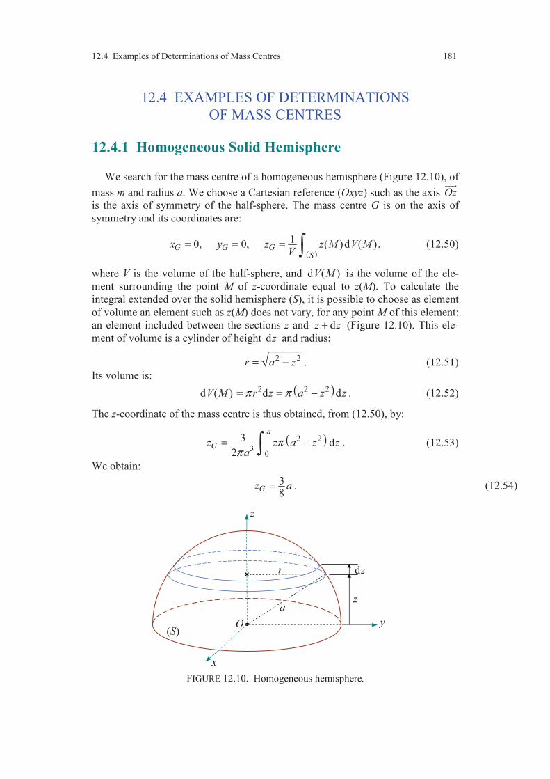
12.4 Examples of Determinations of Mass Centres 181
12.4 EXAMPLES OF DETERMINATIONS
OF MASS CENTRES
12.4.1 Homogeneous Solid Hemisphere
We search for the mass centre of a homogeneous hemisphere (Figure 12.10), of
mass m and radius a. We choose a Cartesian reference (Oxyz) such as the axis Oz
is the axis of symmetry of the half-sphere. The mass centre G is on the axis of
symmetry and its coordinates are:
( )
10, 0, ( )d ( ),G G GS
x y z z M V MV
= = = (12.50)
where V is the volume of the half-sphere, and d ( )V M is the volume of the ele-
ment surrounding the point M of z-coordinate equal to z(M). To calculate the
integral extended over the solid hemisphere (S), it is possible to choose as element
of volume an element such as z(M) does not vary, for any point M of this element:
an element included between the sections z and dz z+ (Figure 12.10). This ele-
ment of volume is a cylinder of height dz and radius:
2 2r a z= − . (12.51)
Its volume is:
( )
2 2 2d ( ) d dV M r z a z zπ π= = − . (12.52)
The z-coordinate of the mass centre is thus obtained, from (12.50), by:
( )
2 2
30
3 d2
a
Gz z a z za
ππ
= − . (12.53)
We obtain:
38
Gz a= . (12.54)
FIGURE 12.10. Homogeneous hemisphere.
(S)
a
r
z
dz
z
y
x
O
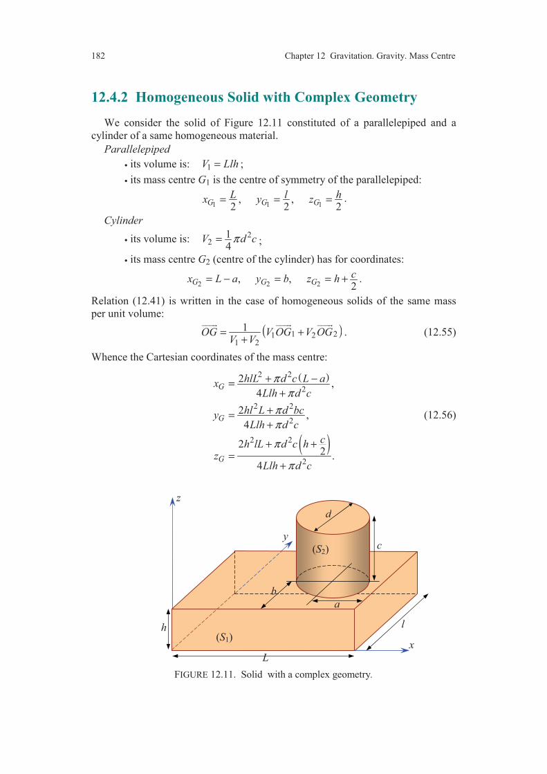
182 Chapter 12 Gravitation. Gravity. Mass Centre
12.4.2 Homogeneous Solid with Complex Geometry
We consider the solid of Figure 12.11 constituted of a parallelepiped and a
cylinder of a same homogeneous material.
Parallelepiped
• its volume is: 1V Llh= ;
• its mass centre G1 is the centre of symmetry of the parallelepiped:
1 1 1, ,
2 2 2G G G
L l hx y z= = = .
Cylinder
• its volume is: 22
14
V d cπ= ;
• its mass centre G2 (centre of the cylinder) has for coordinates:
2 2 2, ,
2G G G
cx L a y b z h= − = = + .
Relation (12.41) is written in the case of homogeneous solids of the same mass
per unit volume:
( )1 21 21 2
1OG V OG V OGV V
= ++
. (12.55)
Whence the Cartesian coordinates of the mass centre:
( )
( )
2 2
2
2 2
2
2 2
2
2 ,4
2 ,4
22 .
4
G
G
G
hlL d c L axLlh d c
hl L d bcyLlh d c
ch lL d c hz
Llh d c
ππ
ππ
π
π
+ −=+
+=+
+ +=
+
(12.56)
FIGURE 12.11. Solid with a complex geometry.
L
(S1)
a
z
y
x
d
c
l
b
(S2)
h
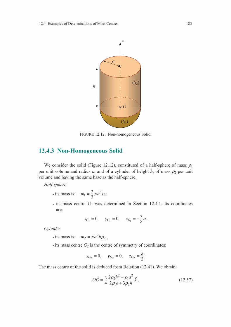
12.4 Examples of Determinations of Mass Centres 183
FIGURE 12.12. Non-homogeneous Solid.
12.4.3 Non-Homogeneous Solid
We consider the solid (Figure 12.12), constituted of a half-sphere of mass ρ1
per unit volume and radius a, and of a cylinder of height h, of mass ρ2 per unit
volume and having the same base as the half-sphere.
Half-sphere
• its mass is: 31 1
23
m aπ ρ= ;
• its mass centre G1 was determined in Section 12.4.1. Its coordinates
are:
1 1 1
30, 0, 8
G G Gx y z a= = = − .
Cylinder
• its mass is: 22 2m a hπ ρ= ;
• its mass centre G2 is the centre of symmetry of coordinates:
2 2 20, 0,
2G G G
hx y z= = = .
The mass centre of the solid is deduced from Relation (12.41). We obtain:
2 22 1
1 2
234 2 3
h aOG k
a h
ρ ρρ ρ
−=
+
. (12.57)
(S1)
z
h
a
O
(S2)
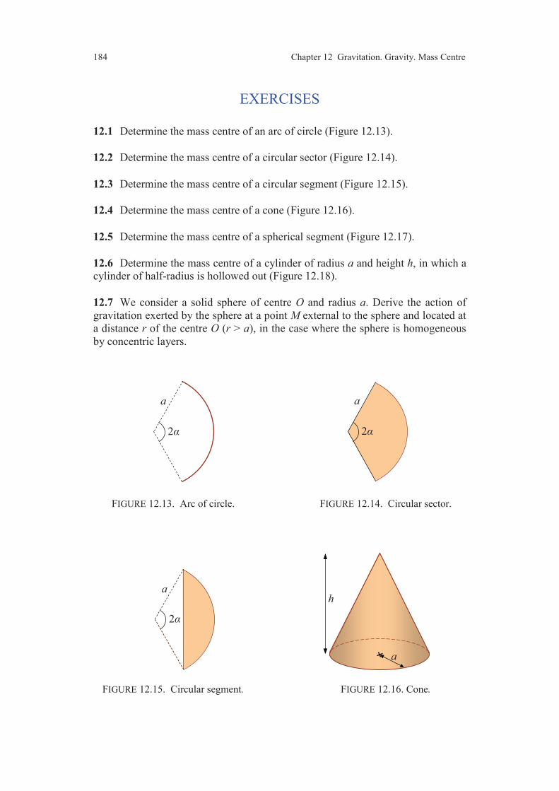
184 Chapter 12 Gravitation. Gravity. Mass Centre
EXERCISES
12.1 Determine the mass centre of an arc of circle (Figure 12.13).
12.2 Determine the mass centre of a circular sector (Figure 12.14).
12.3 Determine the mass centre of a circular segment (Figure 12.15).
12.4 Determine the mass centre of a cone (Figure 12.16).
12.5 Determine the mass centre of a spherical segment (Figure 12.17).
12.6 Determine the mass centre of a cylinder of radius a and height h, in which a
cylinder of half-radius is hollowed out (Figure 12.18).
12.7 We consider a solid sphere of centre O and radius a. Derive the action of
gravitation exerted by the sphere at a point M external to the sphere and located at
a distance r of the centre O (r > a), in the case where the sphere is homogeneous
by concentric layers.
FIGURE 12.13. Arc of circle. FIGURE 12.14. Circular sector.
FIGURE 12.15. Circular segment. FIGURE 12.16. Cone.
2
a
2
a
2
a
h
a

Comments 185
FIGURE 12.17. Spherical segment. FIGURE 12.18. Hollowed cylinder.
COMMENTS
The actions of gravitation are induced by the phenomena of attraction
between masses and are characterized by the Newton’s law. This law
allows us to characterize the action of gravitation exerted by the Earth on a
material body. With the action of gravitation a mechanical action is super-
imposed, induced by the motion of rotation of the Earth around the axis of
the poles South-North. The resultant action is the action of gravity exerted
by the Earth which differs little from the action of gravitation. This action
of gravity exerted on a solid or a set of solids is a force of which the
magnitude is the product of the mass of the solid or set of solids by the
magnitude of the field of the Earth gravity and whose support is the down-
ward vertical axis passing through the mass centre.
Note. The action of gravity is denoted by e in reference to the
corresponding French term “action de pesanteur”.
h
a
h
a

CHAPTER 13
Actions of Contact between Solids Connections
13.1 LAWS OF CONTACT BETWEEN SOLIDS
13.1.1 Introduction
To move on the ground a body (cupboard, case (Figure 13.1), etc.), it is neces-
sary to exert a sufficient mechanical action to overcome the action exerted by the
ground on the body, action which is opposed to any motion of the body on the
ground. The actions of contact between solids are of intermolecular nature and
appear only at this scale. They are thus exerted only at extremely small distances,
hence their name of actions of contact. So the actions of contact are very sensitive
to the state of the surfaces in contact. In addition, the actions of contact depend on
the other mechanical actions which are exerted. For example, it is more difficult
to draw the case filled than the empty case. The phenomena of contact are
complex, and the laws of contact that we shall state are only approximate laws.
They constitute however a satisfactory approach in many problems involving
actions of contact between solids.
FIGURE 13.1. Displacement of a case.

13.1 Laws of Contact between Solids 187
13.1.2 Contact in a Point
13.1.2.1 Laws of Contact in one Point
Let (S) and (T) be two solids, in contact at the point P at a given time (Figure
13.2). In fact the contact occurs between surfaces of very small dimensions and
may be considered as a contact in a point. The two bodies being supposed in-
deformable and impenetrable, they are tangent at the point P. We are in the
kinematic model studied in Chapter 10 (Section 10.1.1).
Owing to the contact of the two bodies at the point P, the body (T) exerts on
the solid (S) an action of contact represented by the torsor T S→
. The laws of
contact in a point are the following ones:
1st law
The action of contact exerted by the solid (T) on the solid (S) is a force of
which the line of action passes through the point of contact P.
The torsor T S→ is thus a slider of which the axis passes through the point
of contact P. In particular:
0P T S =→ . (13.1)
The experimental analysis of the phenomena of contact shows that the resultant
of the action of contact exerted by the solid (T), is not, as in the case of the actions
at distance, known or calculable a priori, but depends on the other mechanical
actions exerted on (S). The action of contact must however verify some conditions
expressed in the laws which we state hereafter.
FIGURE 13.2. Solids in contact in one point.
(S)
(T)
P

188 Chapter 13 Actions of Contact between Solids. Connections
The force of contact exerted by the rigid body (T) on the rigid body (S) is
resolved into two forces:
— a force of resultant tR
, called force of resistance to sliding or force of
friction, of which the line of action is contained in the plan tangent at P to the two
solids;
— a force of resultant nR
called normal force of contact, of which the line of
action is the line normal at the point P to the tangent plane.
The resultant of the action of contact is thus written:
t nR R RT S = +→ . (13.2)
2nd law
If the vector n
is the unit vector of the normal direction at the point P orient-
tated from the solid (T) towards the solid (S), in all the cases where (S) and (T) are
not stuck at the point P, we have:
, with 0,n n nR R n R= ≥
(13.3)
where Rn is the component of the normal force of contact. This law expresses the
fact that the normal force is opposed to the penetration of the solid (S) in the solid
(T). The symbolic representation of the force of contact is reported in Figure 13.3.
3rd law or Coulomb’s law
There exists a positive coefficient f called coefficient of friction of (S) on (T),
dependent on the materials of which (S) and (T) are made, dependent on the state
of the surfaces in contact, but independent of the motions or of the equilibrium of
(S) and (T),such that the following condition is verified at any time:
t nR f R≤
. (13.4)
FIGURE 13.3. Normal and tangential components of the force of contact.
(T)
(S)
P
R
tR
nR
n
tangent plane
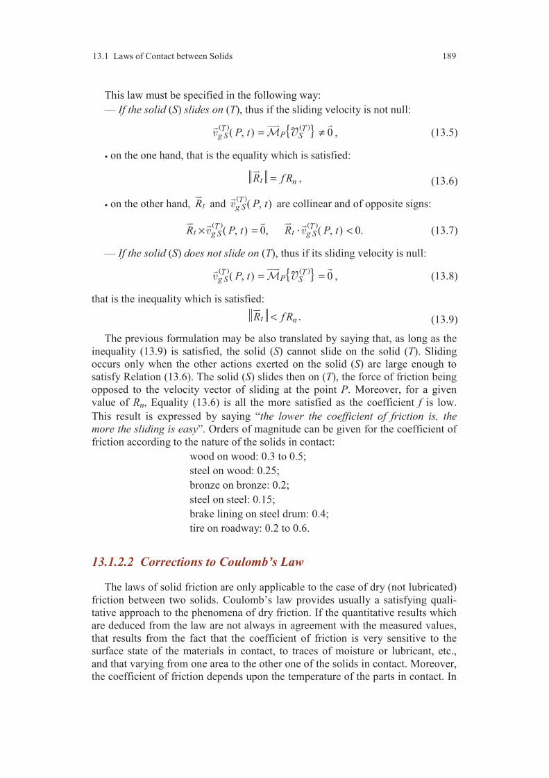
13.1 Laws of Contact between Solids 189
This law must be specified in the following way:
— If the solid (S) slides on (T), thus if the sliding velocity is not null:
( ) ( ) ( , ) 0T TPg S SP t = ≠
, (13.5)
• on the one hand, that is the equality which is satisfied:
t nR f R=
, (13.6)
• on the other hand, tR
and ( )
( , )Tg S P t are collinear and of opposite signs:
( ) ( )
( , ) 0, ( , ) 0.T Tt tg S g SR P t R P t× = <⋅ (13.7)
— If the solid (S) does not slide on (T), thus if its sliding velocity is null:
( ) ( ) ( , ) 0T TPg S SP t = =
, (13.8)
that is the inequality which is satisfied:
t nR f R<
. (13.9)
The previous formulation may be also translated by saying that, as long as the
inequality (13.9) is satisfied, the solid (S) cannot slide on the solid (T). Sliding
occurs only when the other actions exerted on the solid (S) are large enough to
satisfy Relation (13.6). The solid (S) slides then on (T), the force of friction being
opposed to the velocity vector of sliding at the point P. Moreover, for a given
value of Rn, Equality (13.6) is all the more satisfied as the coefficient f is low.
This result is expressed by saying “the lower the coefficient of friction is, the
more the sliding is easy”. Orders of magnitude can be given for the coefficient of
friction according to the nature of the solids in contact:
wood on wood: 0.3 to 0.5;
steel on wood: 0.25;
bronze on bronze: 0.2;
steel on steel: 0.15;
brake lining on steel drum: 0.4;
tire on roadway: 0.2 to 0.6.
13.1.2.2 Corrections to Coulomb’s Law
The laws of solid friction are only applicable to the case of dry (not lubricated)
friction between two solids. Coulomb’s law provides usually a satisfying quali-
tative approach to the phenomena of dry friction. If the quantitative results which
are deduced from the law are not always in agreement with the measured values,
that results from the fact that the coefficient of friction is very sensitive to the
surface state of the materials in contact, to traces of moisture or lubricant, etc.,
and that varying from one area to the other one of the solids in contact. Moreover,
the coefficient of friction depends upon the temperature of the parts in contact. In

190 Chapter 13 Actions of Contact between Solids. Connections
fact the friction increases the temperature of the parts in contact, hence a decrease
of the coefficient of friction. The importance of this effect is highlighted by the
behaviour of car braking, where the friction is higher at the beginning of braking.
The coefficient f also depends to a certain extent on the normal component Rn.
Lastly, the coefficient of friction depends on the sliding velocity.
A way rather simple to take account of the dependence of the coefficient of
friction as a function of speed consists in considering two different values of the
coefficient of friction: a coefficient of static friction fs and a coefficient of
kinematic friction fk, of value lower than that of the static friction. This distinction
between the two conditions of friction then makes it possible to explain some
usual effects. For example, consider a solid resting on an inclined plane. For a
given inclination where the equilibrium is precarious, a very low impulse is
sufficient to break the equilibrium, the body having then an accelerated slippage
motion. If the plane is horizontal, a higher effort is necessary to make move the
solid than that to move it then.
13.1.2.3 Power Developed
The power developed in the reference (T) by the action exerted on the solid
(S), in contact at the point P with (T) is, from (11.13):
( ) ( ) T T
SP T S T S=→ → ⋅ . (13.10)
Thus, when expressed at the point of contact P:
( )
( )( , )T T
g SP R P tT S T S=→ → ⋅
, (13.11)
or since ( )
( , )Tg S P t is orthogonal to nR
:
( )
( )( , )T T
t g SP R P tT S =→ ⋅ . (13.12)
The power developed by the normal force of contact is null. The power is reduced
to that developed by the force of friction. From the Coulomb’s law this power is
negative or null.
13.1.2.4 Contact Without Friction
If friction is necessary in some cases (walk on the ground, entrainment of a car,
etc.), in other cases it is necessary as much as possible to diminish it in order to
decrease the energy dissipated by friction and to avoid a premature attrition of the
parts in contact.
In the extreme case where the coefficient of friction is zero, we will say that the
contact occurs without friction or that the contact is perfect at the point of contact
considered.

13.1 Laws of Contact between Solids 191
In such a description, we have:
0 and t nR R RT S= =→ . (13.13)
The solid (T) exerts on (S) only a normal action of contact. The least action
exerted on the solid (S) will induce sliding of solid (S). Moreover, Expression
(13.12) shows that the power developed is zero.
In conclusion, we will say that the contact between two solids is perfect or
without friction at the point P, if and only if one of the following equivalent con-
ditions is verified:
— the coefficient of friction is zero,
—the action of contact is normal at P to the two solids,
— the power developed by the action of contact is zero.
This model of perfect contact remains however an ideal model, towards which
one tends to approach by polishing the surfaces in contact and lubricating them.
13.1.3 Couples of Rolling and Spinning
13.1.3.1 Introduction
In the preceding section, we studied the case of a contact at a point for which
the action of contact can be reduced to a force of contact. In practice, the contact
between the two solids occurs on a surface localized at the centre P. The action of
contact exerted must then be resolved, at the point P, into a force of contact, of
which the properties were studied in the preceding section 13.1.2, and a couple of
contact of moment-vector
equal to the moment at the point P of the action of
contact:
P T S= → . (13.14)
As the force of contact (Relation (13.2)), the couple is resolved into two
couples:
— a couple of resistance to rolling of moment-vector t
, of which the
direction is contained in the plane tangent in P to the two solids;
— a couple of resistance to spinning of moment-vector n
of direction
orthogonal to the tangent plane.
The moment-vector is thus written:
t n= +
. (13.15)
The properties of the couples of contact are complex. Laws similar to the
Coulomb’s law are however stated for the qualitative analysis of the phenomena
of rolling and spinning.
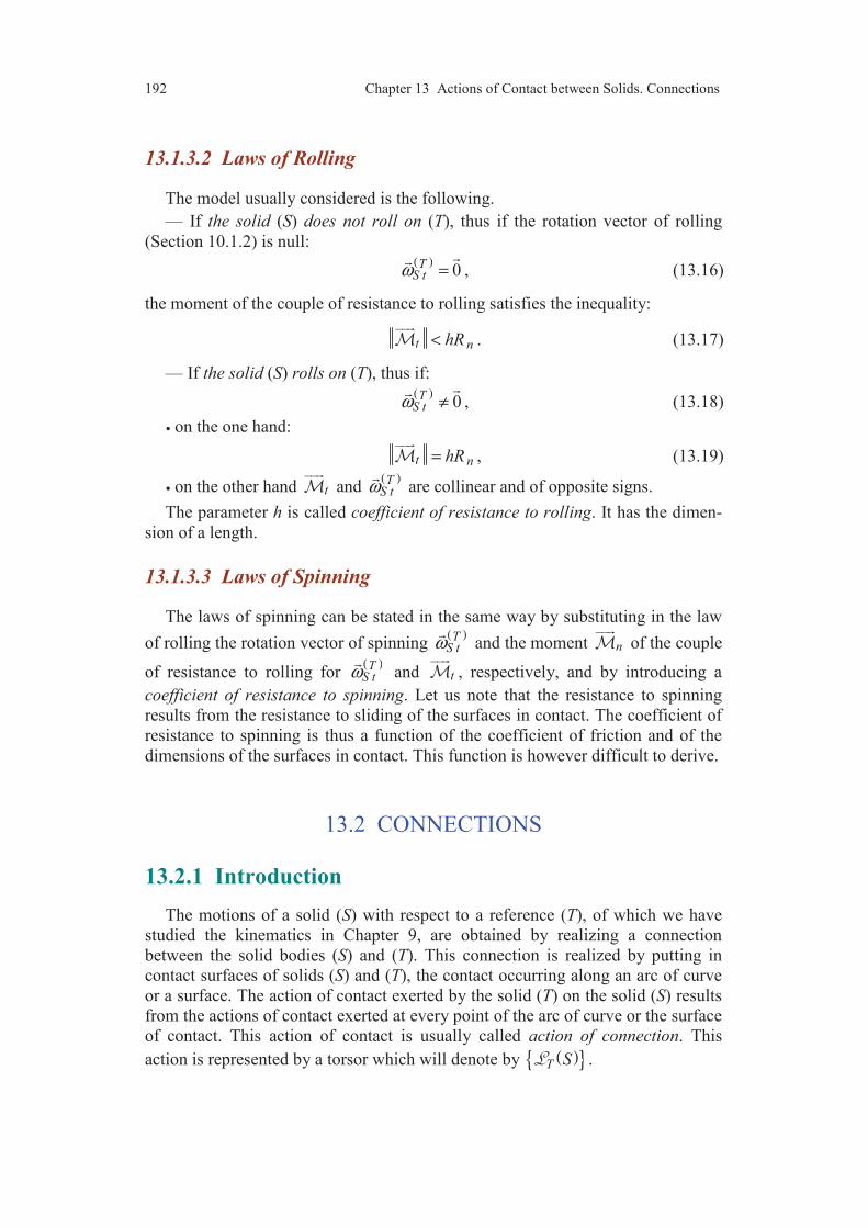
192 Chapter 13 Actions of Contact between Solids. Connections
13.1.3.2 Laws of Rolling
The model usually considered is the following.
— If the solid (S) does not roll on (T), thus if the rotation vector of rolling
(Section 10.1.2) is null: ( )
0TS tω =
, (13.16)
the moment of the couple of resistance to rolling satisfies the inequality:
t nhR<
. (13.17)
— If the solid (S) rolls on (T), thus if: ( )
0TS tω ≠
, (13.18)
• on the one hand:
t nhR=
, (13.19)
• on the other hand t
and ( )TS tω
are collinear and of opposite signs.
The parameter h is called coefficient of resistance to rolling. It has the dimen-
sion of a length.
13.1.3.3 Laws of Spinning
The laws of spinning can be stated in the same way by substituting in the law
of rolling the rotation vector of spinning ( )TS tω
and the moment n
of the couple
of resistance to rolling for ( )TS tω
and t
, respectively, and by introducing a
coefficient of resistance to spinning. Let us note that the resistance to spinning
results from the resistance to sliding of the surfaces in contact. The coefficient of
resistance to spinning is thus a function of the coefficient of friction and of the
dimensions of the surfaces in contact. This function is however difficult to derive.
13.2 CONNECTIONS
13.2.1 Introduction
The motions of a solid (S) with respect to a reference (T), of which we have
studied the kinematics in Chapter 9, are obtained by realizing a connection
between the solid bodies (S) and (T). This connection is realized by putting in
contact surfaces of solids (S) and (T), the contact occurring along an arc of curve
or a surface. The action of contact exerted by the solid (T) on the solid (S) results
from the actions of contact exerted at every point of the arc of curve or the surface
of contact. This action of contact is usually called action of connection. This
action is represented by a torsor which will denote by ( ) T S .
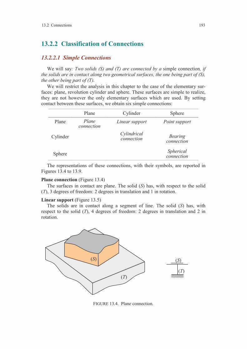
13.2 Connections 193
13.2.2 Classification of Connections
13.2.2.1 Simple Connections
We will say: Two solids (S) and (T) are connected by a simple connection, if
the solids are in contact along two geometrical surfaces, the one being part of (S),
the other being part of (T).
We will restrict the analysis in this chapter to the case of the elementary sur-
faces: plane, revolution cylinder and sphere. These surfaces are simple to realize,
they are not however the only elementary surfaces which are used. By setting
contact between these surfaces, we obtain six simple connections:
Plane Cylinder Sphere
Plane Plane connection
Linear support Point support
Cylinder Cylindrical connection
Bearing connection
Sphere Spherical
connection
The representations of these connections, with their symbols, are reported in
Figures 13.4 to 13.9.
Plane connection (Figure 13.4)
The surfaces in contact are plane. The solid (S) has, with respect to the solid
(T), 3 degrees of freedom: 2 degrees in translation and 1 in rotation.
Linear support (Figure 13.5)
The solids are in contact along a segment of line. The solid (S) has, with
respect to the solid (T), 4 degrees of freedom: 2 degrees in translation and 2 in
rotation.
FIGURE 13.4. Plane connection.
(S)
(T)
(T)
(S)
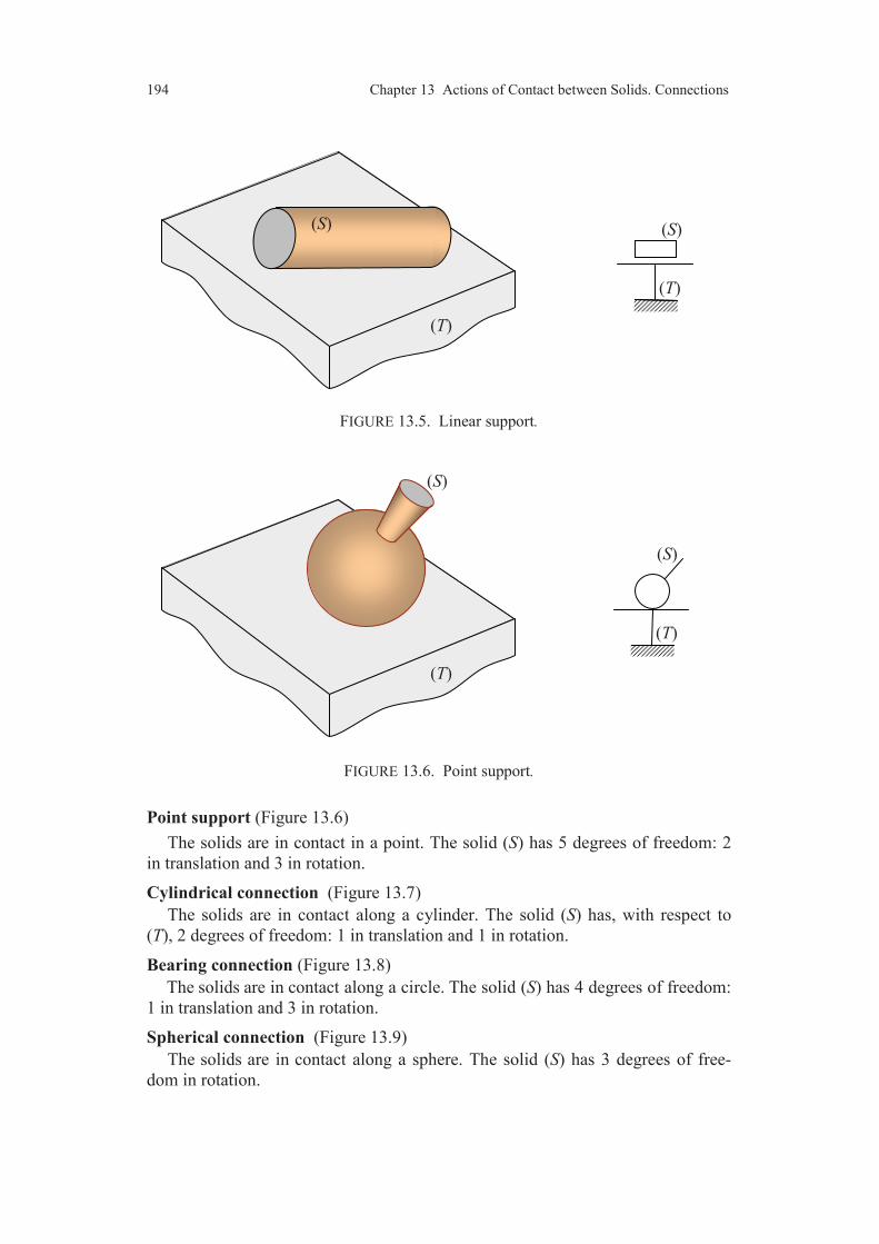
194 Chapter 13 Actions of Contact between Solids. Connections
FIGURE 13.5. Linear support.
FIGURE 13.6. Point support.
Point support (Figure 13.6)
The solids are in contact in a point. The solid (S) has 5 degrees of freedom: 2
in translation and 3 in rotation.
Cylindrical connection (Figure 13.7)
The solids are in contact along a cylinder. The solid (S) has, with respect to
(T), 2 degrees of freedom: 1 in translation and 1 in rotation.
Bearing connection (Figure 13.8)
The solids are in contact along a circle. The solid (S) has 4 degrees of freedom:
1 in translation and 3 in rotation.
Spherical connection (Figure 13.9)
The solids are in contact along a sphere. The solid (S) has 3 degrees of free-
dom in rotation.
(T)
(S)
(T)
(S)
(T)
(S)
(T)
(S)
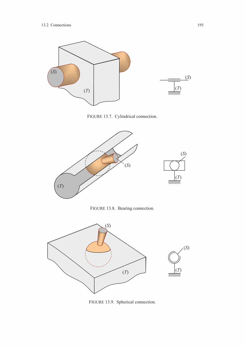
13.2 Connections 195
FIGURE 13.7. Cylindrical connection.
FIGURE 13.8. Bearing connection.
FIGURE 13.9. Spherical connection.
(T)
(S)
(T)
(S)
(T)
(S) (S)
(T)
(T)
(S)
(S)
(T)
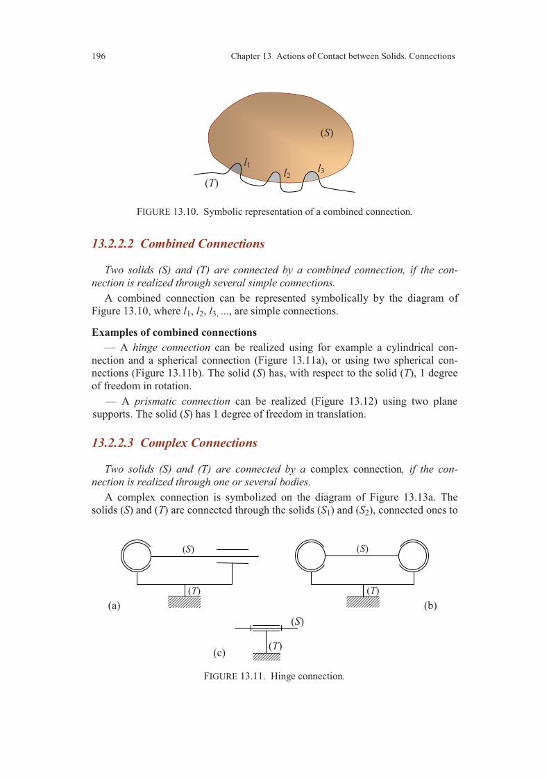
196 Chapter 13 Actions of Contact between Solids. Connections
FIGURE 13.10. Symbolic representation of a combined connection.
13.2.2.2 Combined Connections
Two solids (S) and (T) are connected by a combined connection, if the con-
nection is realized through several simple connections.
A combined connection can be represented symbolically by the diagram of
Figure 13.10, where l1, l2, l3, ..., are simple connections.
Examples of combined connections — A hinge connection can be realized using for example a cylindrical con-
nection and a spherical connection (Figure 13.11a), or using two spherical con-
nections (Figure 13.11b). The solid (S) has, with respect to the solid (T), 1 degree
of freedom in rotation.
— A prismatic connection can be realized (Figure 13.12) using two plane
supports. The solid (S) has 1 degree of freedom in translation.
13.2.2.3 Complex Connections
Two solids (S) and (T) are connected by a complex connection, if the con-
nection is realized through one or several bodies.
A complex connection is symbolized on the diagram of Figure 13.13a. The
solids (S) and (T) are connected through the solids (S1) and (S2), connected ones to
FIGURE 13.11. Hinge connection.
(S)
(T)
l1
l2l3
(S)
(T)
(S)
(T)
(T)
(S)
(a) (b)
(c)
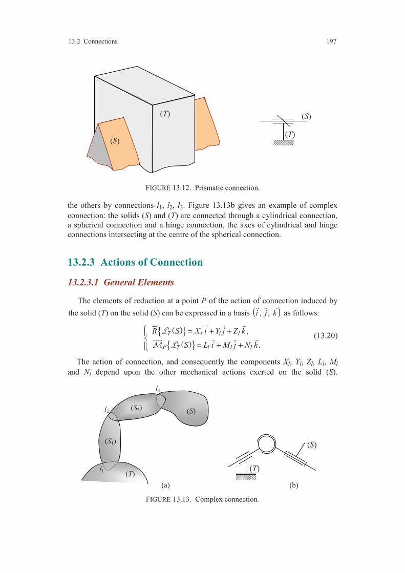
13.2 Connections 197
FIGURE 13.12. Prismatic connection.
the others by connections l1, l2, l3. Figure 13.13b gives an example of complex
connection: the solids (S) and (T) are connected through a cylindrical connection,
a spherical connection and a hinge connection, the axes of cylindrical and hinge
connections intersecting at the centre of the spherical connection.
13.2.3 Actions of Connection
13.2.3.1 General Elements
The elements of reduction at a point P of the action of connection induced by
the solid (T) on the solid (S) can be expressed in a basis ( ), , i j k
as follows:
( ) ( )
,
.
T l l l
P T l l l
R S X i Y j Z k
S L i M j N k
= + +
= + +
(13.20)
The action of connection, and consequently the components Xl, Yl, Zl, Ll, Ml
and Nl depend upon the other mechanical actions exerted on the solid (S).
FIGURE 13.13. Complex connection.
(T)
(S) (T)
(S)
(a)
(T)
(S)
(b)
l1
l2
l3
(S1)
(S2) (S)
(T)

198 Chapter 13 Actions of Contact between Solids. Connections
However, to solve the problems of Mechanics of rigid bodies, it is necessary to
introduce assumptions on some of the components according to the physical
nature of the connections: connection without friction, connection with dry fric-
tion or viscous friction.
13.2.3.2 Power Developed by the Actions of Connection
The power developed in the reference (T) by the action of connection exerted
by the solid (T) on the solid (S) is from (11.13):
( ) ( ) ( ) ( ) T TT T SP S S= ⋅ , (13.21)
where ( ) TS is the kinematic torsor relative to the motion of the solid (S) with
respect to the solid (T).
By introducing the elements of reduction at the point P of the action of con-
nection (13.20), the preceding relation is written:
( ) ( ) ( ) ( ) ( ) ( ) T T TP PT T TS SP S R S S R= +⋅ ⋅
, (13.22)
or ( ) ( ) ( ) ( ) ( )
( , )T TPT T T SP S R S P t S ω= + ⋅⋅
, (13.23)
by introducing the veloctity vector of the point P and the instantaneous rotation
vector.
13.2.4 Connection Without Friction
13.2.4.1 Model of Perfect Connection
So as to reduce the dissipated energy and to decrease the attrition of the sur-
faces in contact, it is necessary to obtain surfaces such as the contact in every
point approach as much as possible a perfect contact. We will say that a con-
nection between two solids is perfect, if the contact between the solids is perfect
in every point. By extension of the results established in Subsection 13.1.2.4, we
deduce then:
A connection is perfect, if and only if the power developed by the action of
connection is null.
We will consider this property as the definition of a perfect connection. The
model of perfect connection is however only an idealized model, towards which
we usually tend to approach in the technological realizations.
13.2.4.2 Hinge Connection
In the case of a hinge connection, the solid (S) is animated, with respect to the
reference (T), by a motion of rotation about the axis of the hinge connection. This
motion was studied in Section 9.4.1. The solid (S) has one degree of freedom in
13.2 Connections 199
rotation ψ and the kinematic torsor is defined (Section 9.4.1.2) by its elements of
reduction at an arbitrary point OS of the axis of rotation:
( ) ( )
( ) ( )
,
( , ) 0.S
T TS S
T TO S S
R k
O t
ω ψ = =
= =
(13.24)
The power developed, in the reference (T), by the action of connection is from
(13.23): ( ) ( ) ( ) ( )
S
T TOT T S lP S S Nω ψ= ⋅ =
. (13.25)
The condition of perfect connection is then written:
( ) ( ) 0, TT lP S N ψ ψ= = ∀ . (13.26)
Thus:
0lN = . (13.27)
Hence the result:
If the solid (S) is connected to the solid (T) by a perfect hinge connection, of
axis of unit direction vector k
, the action exerted by (T) on (S) is represented by
a torsor having in a basis ( ), , i j k
:
—an arbitrary resultant of components Xl, Yl, Zl ;
— a moment at an arbitrary point of the axis of the hinge connection which is
orthogonal to the direction of this axis, thus of components Ll , Ml, 0.
We write the result in the form:
( ) , , , , , 0 ,SS
T l l l l l OOS X Y Z L M= (13.28)
where OS is an arbitrary point of the axis of the connection. The components Xl,
..., Ml, depend upon the other mechanical actions exerted on the solid (S).
13.2.4.3 Prismatic Connection
In the case of a prismatic connection, the solid (S) moves with a rectilinear
translation motion. If i
is the direction of the prismatic connection, the solid (S)
has one degree of freedom in x (abscissa of an arbitrary point P of the solid (S)).
The elements of reduction at the point P of the kinematic torsor are:
( ) ( )
( ) ( ) ( )
0,
( , ) , .
T TS S
T TP S
R
P t x i P S
ω = =
= = ∀ ∈
(13.29)
The power developed, in the reference (T), by the action of connection is:
( ) ( ) ( ) ( )( , )T T
T T lP S R S P t X x= =⋅
. (13.30)
The condition of perfect connection is thus written:
0lX = . (13.31)

200 Chapter 13 Actions of Contact between Solids. Connections
Hence the result:
If the solid (S) is connected to the solid (T) by a perfect prismatic connection of
direction i
, the action exerted by (T) on (S) is represented by a torsor having in
a basis ( ), , i j k
:
— a resultant orthogonal to i
, hence of components 0, Yl, Zl,;
— an arbitrary moment of components Ll, Ml, Nl whatever the point of the
solid (S).
Thus:
( ) 0, , , , , ,T l l l l l PPS Y Z L M N= (13.32)
where P is an arbitrary point of the solid (S).
13.2.4.4 Cylindrical Connection
In the case where the solid (S) is connected to the solid (T) by a cylindrical
connection of direction k
, the solid (S) has (Section 9.4.3) one degree of freedom
in translation z (abscissa of an arbitrary point OS of the axis of the cylindrical
connection) and one degree of freedom in rotation ψ. The elements of reduction at
point OS of the kinematic torsor (Relations (9.66) and (9.67)) are:
( ) ( )
( ) ( )
,
( , ) .S
T TS S
T TO S S
R k
O t z k
ω ψ = =
= =
(13.33)
The power developed, in the reference (T), by the action of connection is from
(13.23): ( ) ( ) T
T l lP S Z z N ψ= + (13.34)
The condition of perfect connection is thus written:
0, , .l lZ z N zψ ψ+ = ∀ (13.35)
Hence:
0, 0.l lZ N= = (13.36)
Hence the result:
If the solid (S) is connected to the solid (T) by a perfect cylindrical connection
of axis of direction k
, the action exerted by (T) on (S) is represented by a torsor
having in a basis ( ), , i j k
:
— a resultant of components Xl, Yl, 0 ;
— a moment of components Ll, Ml, 0, at an arbitrary point of the axis of the
cylindrical connection.
This result may be written in the form:
( ) , , 0, , , 0 ,SS
T l l l l OOS X Y L M= (13.37)
where OS is an arbitrary point of the axis of the connection. The components Xl,
Yl, Ll, and Ml depend upon the other mechanical actions exerted on the solid (S).
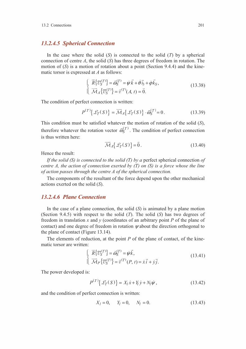
13.2 Connections 201
13.2.4.5 Spherical Connection
In the case where the solid (S) is connected to the solid (T) by a spherical
connection of centre A, the solid (S) has three degrees of freedom in rotation. The
motion of (S) is a motion of rotation about a point (Section 9.4.4) and the kine-
matic torsor is expressed at A as follows:
( ) ( )
( ) ( )
3 ,
( , ) 0.
T TS S S
T TA S
R k i k
A t
ω ψ θ ϕ = = + +
= =
(13.38)
The condition of perfect connection is written:
( ) ( ) ( ) ( )0T T
AT T SP S S ω= ⋅ = . (13.39)
This condition must be satisfied whatever the motion of rotation of the solid (S),
therefore whatever the rotation vector ( )TSω
. The condition of perfect connection
is thus written here:
( ) 0A T S =
. (13.40)
Hence the result:
If the solid (S) is connected to the solid (T) by a perfect spherical connection of
centre A, the action of connection exerted by (T) on (S) is a force whose the line
of action passes through the centre A of the spherical connection.
The components of the resultant of the force depend upon the other mechanical
actions exerted on the solid (S).
13.2.4.6 Plane Connection
In the case of a plane connection, the solid (S) is animated by a plane motion
(Section 9.4.5) with respect to the solid (T). The solid (S) has two degrees of
freedom in translation x and y (coordinates of an arbitrary point P of the plane of
contact) and one degree of freedom in rotation ψ about the direction orthogonal to
the plane of contact (Figure 13.14).
The elements of reduction, at the point P of the plane of contact, of the kine-
matic torsor are written:
( ) ( )
( ) ( )
,
( , ) .
T TS S
T TP S
R k
P t x i y j
ω ψ = =
= = +
(13.41)
The power developed is:
( ) ( ) TT l l lP S X x Y y N ψ= + + , (13.42)
and the condition of perfect connection is written:
0, 0, 0.l l lX Y N= = = (13.43)
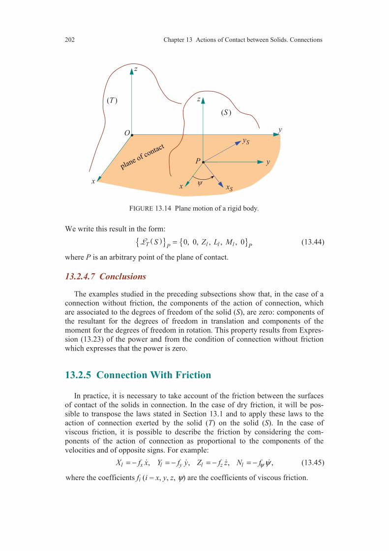
202 Chapter 13 Actions of Contact between Solids. Connections
FIGURE 13.14 Plane motion of a rigid body.
We write this result in the form:
( ) 0, 0, , , , 0T l l l PPS Z L M= (13.44)
where P is an arbitrary point of the plane of contact.
13.2.4.7 Conclusions
The examples studied in the preceding subsections show that, in the case of a
connection without friction, the components of the action of connection, which
are associated to the degrees of freedom of the solid (S), are zero: components of
the resultant for the degrees of freedom in translation and components of the
moment for the degrees of freedom in rotation. This property results from Expres-
sion (13.23) of the power and from the condition of connection without friction
which expresses that the power is zero.
13.2.5 Connection With Friction
In practice, it is necessary to take account of the friction between the surfaces
of contact of the solids in connection. In the case of dry friction, it will be pos-
sible to transpose the laws stated in Section 13.1 and to apply these laws to the
action of connection exerted by the solid (T) on the solid (S). In the case of
viscous friction, it is possible to describe the friction by considering the com-
ponents of the action of connection as proportional to the components of the
velocities and of opposite signs. For example:
, , , ,l x l y l z lX f x Y f y Z f z N fψ ψ= − = − = − = − (13.45)
where the coefficients fi (i = x, y, z, ψ) are the coefficients of viscous friction.
z
O
(T )
y
z
P y
x
yS
xS
(S )
x

Comments 203
COMMENTS
Connections have a particular importance within the framework of the
design of mechanical systems. Thus, the reader will have to pay a close
attention to the concepts developed in the present chapter. As application
of the general concepts, this chapter considers the cases of connections
between solids using elementary connections. The reader must have assi-
milated well the elements developed in this context.
Contrary to the actions at distance, the actions of contact depend upon
the other actions exerted on the solid or the system of solids under consi-
deration. These conditions are easily derived, in the case of connections
without friction, by writing the nullity of the power developed in the
motion of the solid in connection. To take account of the conditions of
friction, the model simplest to treat is that of viscous friction where the
components of the actions of connections are proportional to the compo-
nents of the velocities and of opposite signs. Dry friction is usually rather
difficult to analyze. The behaviour is transposed from the friction law of
Coulomb which is stated in the case of two solids in contact in a point and
from the laws of rolling and spinning friction.
Note. The actions of connections are denoted by ( )T S in reference to
the corresponding French term “actions de liaisons”.

CHAPTER 14
Statics of Rigid Bodies
14.1 INTRODUCTION
The purpose of this chapter is to analyze the mechanical actions exerted on a
material system, through the study of the equilibrium of a rigid body or a system
of rigid bodies.
A system of rigid bodies is in equilibrium with respect to a given reference, if
during time every point of the system keeps a fixed position with respect to the
reference.
The laws of statics are a consequence of the fundamental principle of dynamics
which will state in Chapter 18.
14.2 LAW OF STATICS
14.2.1 Case of a Rigid Body
A solid (S) submitted to mechanical actions is in equilibrium, if and only if the
torsor representing the whole of the mechanical actions exerted on the solid is the
null torsor.
Thus:
( ) 0S = , (14.1)
with
( ) S S S= → .
The mechanical actions exerted on a solid can be divided into:
— known or calculable actions (actions of gravitation or gravity, electro-
magnetic actions) represented by the torsor ( ) S ;

14.2 Laws of Statics 205
— actions of connections, depending on the other actions exerted on the solid
(S), represented by the torsor ( ) S .
The law of statics for the solid (S) is thus written:
( ) ( ) 0S S =+ . (14.2)
This relation leads to two vector equations:
— the equation of the resultant:
( ) ( ) 0R S R S =+ , (14.3)
— the equation of the moment at any point P:
( ) ( ) 0P PS S =+ . (14.4)
The equilibrium of a solid thus provides 6 scalar equations of which the reso-
lution will be made easier by a discerning choice of the point P and bases in
which the resultant and the moment will be expressed.
14.2.2 Case of a Set of Rigid Bodies
A set of rigid bodies is in equilibrium if and only if every rigid body is in
equilibrium.
We consider the set (D) constituted of n solids: 1 2( ), ( ), . . . , ( ),iS S S . . . ,
( ), . . . , ( ).j nS S The actions exerted on the solid (Si) are divided into:
— external actions, actions exerted by the exterior of (D):
( ) ( ) ( ) i i i iD S S S S→ = = + , (14.5)
known (or calculable) actions actions of connections
exerted by the exterior of (D) with the exterior of (D)
— internal actions, exerted by the other solids of (D):
( ) ( ) ( ) 1 1 1
n n n
j i j i j i j i
j j ji i i
S S S S S
= = =≠ ≠ ≠
→ = = + . (14.6)
known actions exerted actions of connections
by the other solids (Sj) with the solids (Sj)
The equilibrium of each solid (Si) is thus written in one of the forms:
1
0
n
i j i
ji
D S S S
=≠
→ + → = , (14.7)
or

206 Chapter 14 Statics of Rigid Bodies
( ) ( ) ( ) ( )
1
,0
for 1, 2, . . . , .
n
i i j i j i
ji
S S S S
i n
=≠
+ + + =
=
(14.8)
The equilibrium of the set (D) thus leads to n equations of torsors, 2n vector equa-
tions and 6n scalar equations.
Some equations, linear combinations of the preceding ones, may be obtained
by considering the equilibrium of a part of the set (D). These equations will be
able, in some cases, to replace some of Equations (14.7) or (14.8) advantageously.
In particular, it is possible to write the global equilibrium of the set (D), thus:
0D D→ = , (14.9)
or from (11.4):
1
0
n
i
i
D S
=
→ = . (14.10)
This equation introduces only the actions external to the set (D).
14.2.3 Mutual Actions
We consider two materials set (D1) and (D2) which are disjoint. The mecha-
nical actions exerted on the set (D1) are represented by the torsor:
1 1 2 11 2 1D D D DD D D→ = + →∪ → . (14.11)
The mechanical actions exerted on the set (D2) are:
2 2 1 21 2 2D D D DD D D→ = + →∪ → . (14.12)
The equilibrium of each set (D1) and (D2) is written:
1 1 0D D→ = , (14.13)
2 2 0D D→ = . (14.14)
The equilibrium of the set ( )1 2D D∪ is written:
1 2 1 2 0D D D D =∪ → ∪ , (14.15)
or
1 2 1 1 2 2 0D D D D D D+ =∪ → ∪ → . (14.16)
The association of the preceding relations leads to the relation:
2 1 1 2D D D D→ = − → . (14.17)
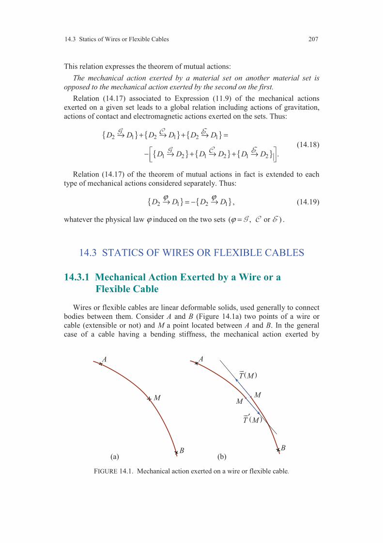
14.3 Statics of Wires or Flexible Cables 207
This relation expresses the theorem of mutual actions:
The mechanical action exerted by a material set on another material set is
opposed to the mechanical action exerted by the second on the first.
Relation (14.17) associated to Expression (11.9) of the mechanical actions
exerted on a given set leads to a global relation including actions of gravitation,
actions of contact and electromagnetic actions exerted on the sets. Thus:
2 12 1 2 1
1 21 2 1 2 .
D DD D D D
D DD D D D
→+ + =→ →
→− + +→ →
(14.18)
Relation (14.17) of the theorem of mutual actions in fact is extended to each
type of mechanical actions considered separately. Thus:
2 1 2 1D D D Dϕ ϕ→ →= − , (14.19)
whatever the physical law ϕ induced on the two sets ( ,ϕ = or ) .
14.3 STATICS OF WIRES OR FLEXIBLE CABLES
14.3.1 Mechanical Action Exerted by a Wire or a Flexible Cable
Wires or flexible cables are linear deformable solids, used generally to connect
bodies between them. Consider A and B (Figure 14.1a) two points of a wire or
cable (extensible or not) and M a point located between A and B. In the general
case of a cable having a bending stiffness, the mechanical action exerted by
FIGURE 14.1. Mechanical action exerted on a wire or flexible cable.
M
A
B
M
A
B
M
( )T M
( )T M′
(a) (b)

208 Chapter 14 Statics of Rigid Bodies
the part AM on the part MB is arbitrary and can be resolved into a force and a
couple depending on the point M.
We say that wire (or cable) is flexible, if and only if the couple which is exerted
is null at any point of wire (or cable).
The mechanical action exerted by the part AM on the part MB is thus a force,
called tension at the point M, of which the support passes through the point M and
the resultant ( )T M
depends on the point M. Moreover, it is possible to show and
experiment confirms that:
The line of action of the force exerted by the part AM on the part BM coincides
with the tangent at M to the wire or cable, orientated from B towards M (Figure
14.1b).
The roles of A and B can be exchanged, and so the part BM exerts on the part
AM a force of resultant ( )T M′ collinear to the preceding one but of opposite sign:
( ) ( ), with 0T M T Mα α′ = − >
. (14.20)
14.3.2 Equation of Statics of a Wire
Consider an element ds MM ′= of wire (Figure 14.2). The resultant of the
forces of tension which are exerted on this element is:
d( d ) ( ) d d
d
TT s s T s T s
s+ − = =
. (14.21)
The equilibrium of the element is written:
dd d 0
dl
Ts s g
sρ+ =
, (14.22)
by introducing the mass by unit length ρl of the wire and g
the field of gravity
induced by the Earth. Hence the equilibrium equation of the wire:
1 d0
dl
Tg
sρ+ =
. (14.23)
FIGURE 14.2. Mechanical action exerted on an element of wire.
M
A
B
M'
M'
M
T
te
ne

14.3 Statics of Wires or Flexible Cables 209
The tension of the wire at the point M is written:
tT T e=
, (14.24)
hence:
d d
d dt n
T T Te e
s s= +
, (14.25)
by introducing the unit vectors ( ), t ne e
of the tangent and principal normal
directions, and the radius of curvature of the wire at the point M. The equi-
librium equation (14.23) of the wire thus can be written in the form:
( )1 d0
dt n
l
T Tg e e
sρ+ + =
. (14.26)
In the case of a wire of negligible mass, the equilibrium equation (14.22) of the
element is reduced to:
d0
d
T
s=
. (14.27)
This relation shows that:
If the tensions at A and B are not null, the tension exerted by the portion AM on
the portion MB has the same resultant, whatever the point M of AB. The portion
AB of the wire is rectilinear.
14.3.3 Wire or Flexible Cable Submitted to the Gravity
We search for the shape which is getting by a wire or a flexible cable of homo-
geneous linear mass submitted to the action of gravity. We choose (Figure 14.3) a
frame of reference (Oxyz) so that the axis Oy
is upward vertical and the points A
and B of the wire are contained in the plane Oxy. The equation of equilibrium
(14.23) leads, while introducing the angle α between the tangent at M to the curve
and the axis Ox
, to two equations:
FIGURE 14.3. Wire submitted to the action of gravity.
M
A B
T
y
xO
a
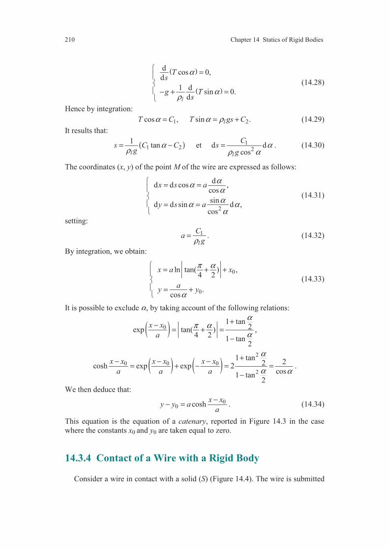
210 Chapter 14 Statics of Rigid Bodies
( )
( )
dcos 0,
d
1 dsin 0.
dl
Ts
g Ts
α
αρ
= − + =
(14.28)
Hence by integration:
1 2cos , sin .lT C T gs Cα α ρ= = + (14.29)
It results that:
( )
11 2 2
1tan et d d
cosl l
Cs C C s
g gα α
ρ ρ α= − = . (14.30)
The coordinates (x, y) of the point M of the wire are expressed as follows:
2
dd d cos ,
cos
sind d sin d ,
cos
x s a
y s a
αααα
α αα
= = = =
(14.31)
setting:
1
l
Ca
gρ= . (14.32)
By integration, we obtain:
0
0
ln tan( ) ,4 2
.cos
x a x
ay y
π α
α
= + + = +
(14.33)
It is possible to exclude α, by taking account of the following relations:
( )01 tan
2exp tan( )4 2
1 tan2
x x
a
απ α
α
+−= + =
−,
( ) ( )2
0 0 0
2
1 tan22cosh exp exp 2
cos1 tan
2
x x x x x x
a a a
α
α α
+− − −= + − = =
−.
We then deduce that:
00 cosh
x xy y a
a
−− = . (14.34)
This equation is the equation of a catenary, reported in Figure 14.3 in the case
where the constants x0 and y0 are taken equal to zero.
14.3.4 Contact of a Wire with a Rigid Body
Consider a wire in contact with a solid (S) (Figure 14.4). The wire is submitted

14.3 Statics of Wires or Flexible Cables 211
at its points A and B to tensions TA and TB, respectively. The contact with the solid
(S) occurs between the points M1 and M2. Any element ds of the wire is
submitted to a force of contact, which can be resolved (13.2) into a force of
friction of resultant tR
and a normal force of resultant nR
. In the case where the
action of gravity can be neglected compared to the other actions exerted on the
element of wire, the equation of equilibrium (14.23) is modified as:
d0
dt n
TR R
s+ + =
, (14.35)
or by introducing the components Rt and Rn of the force of friction and the normal
force:
d0
dt t n n
TR e R e
s+ + =
, (14.36)
where te
and ne
are the unit vectors of the tangent and the normal at M to the wire
(Figure 14.4). Taking account of Relation (14.25), the equation of equilibrium
leads to the two equations:
d0
dt
TR
s+ = , (14.37)
d0 or 0
dn n
TR T R
s
α+ = + =
, (14.38)
where T is the magnitude of the tension of the wire at point M and α the angle
between the direction te
and the direction 1AM
of the wire at point M1.
1. In the case where there is no friction with the solid (S): Rt = 0, and Relation
(14.37) shows that the magnitude of the tension is maintained along the wire.
2. In the case where friction is induced between the solid (S) and the wire, cha-
racterized by a coefficient of friction f, Coulomb’s law involves that equilibrium
FIGURE 14.4. Wire in contact with a rigid body.
A
B
AT
BT
te
ne
M
M1M2
2
(S)

212 Chapter 14 Statics of Rigid Bodies
is maintained as long as:
t nR f R< , (14.39)
or from (14.37) and (14.38):
d d
d d
Tf T
s s
α< . (14.40)
The ultimate equilibrium is thus obtained when:
d d
d
Tf
T s
α= . (14.41)
Thus, integrating between the points M1 and M2:
2fB AT T e α= , (14.42)
where α2 is the winding angle at the point M2, evaluated from the point M1.
For a coefficient of friction of 0.25, and for 3 winding turns (α2 = 6π), we find
111B AT T≈ . The tension to be exerted at B to cause sliding of the wire on the
solid is thus much higher than the tension exerted at A. This result is extensively
used in practice, for example for mooring of the boats.
14.4 EXAMPLES OF EQUILIBRIUM
14.4.1 Case of a Rigid Body
We consider the device of Figure 14.5. A crank can turn about a horizontal axis
BE. This axis is connected to the frame (T) through two connections of respective
centres C and E. A pulley of centre D, rigidly locked with the crank, is connected
to a mass M through a flexible wire and a second pulley attached to the frame.
The position of the frame is defined by the value α of the angle between AB and
the horizontal direction (Figure 14.5b). To maintain the equilibrium of the crank,
it is exerted at the extremity A a force of magnitude F and of support having a
direction β with respect to the direction BA
(Figure 14.5b). The pulley of centre
D has a radius R and a mass m. The mass of the crank ABE is negligible compared
to the masses M and m. The nature of the connections at points C and E is to be
defined so that the system is entirely determined. Thus, it is said that the system is
isostatic.
14.4.1.1 Analysis of the Mechanical Actions Exerted on the Crank
We denote: AB = a, BC = b, CD = d1, DE = d2, and γ the angle between the
vertical direction and the wire connected to the pulley.
As coordinate system attached to the crank-pulley set (S), we choose the
system (Bxyz), such as the axis Bz
coincides BE the axis Bx
is horizontal. The

14.4 Examples of Equilibrium 213
FIGURE 14.5. Equilibrium of a crank-pulley system.
Cartesian coordinates of the different points are then:
( ) ( ) ( )
( ) ( ) ( )1 1 2 1
cos , sin , 0 , 0, 0, 0 , 0, 0, ,
0, 0, , 0, 0, , cos , sin , .
A a a B C b
D b d E b d d F R R b d
α α
γ γ+ + + +
1. Action of gravity The action of gravity exerted on the pulley is represented by the torsor
( ) e S whose the elements of reduction at the point D are:
( )
( )
e ,
e 0.D
R S mg j
S
= −
=
2. Force exerted at the point A
The force is represented by the torsor ( ) S of elements of reduction:
( ) ( ) ( )
( )
cos sin ,
0.A
R S F i j
S
α β α β = + + +
=
A
B
y
x
C
D
E
F
z
a
b
d1
d2
M(a)
B
A
F
x
y
horizontal (b)

214 Chapter 14 Statics of Rigid Bodies
FIGURE 14.6. Tension exerted by the wire on the pulley.
3. Action exerted by the wire at F
The wire being flexible, it transmits entirely the action of gravity exerted by the
mass M. This action is a force of which the direction of the support is given by
that of the wire (Figure 14.6). The action is represented by the torsor ( ) f S :
( ) ( )
( )
sin cos ,
0.
f
F f
R S Mg u Mg i j
S
γ γ = = − +
=
4. Action exerted by the frame at the level of the connection in C
It is represented by the torsor ( ) C S of elements of reduction at the point C:
( ) ( )
,
.
C C C C
C C C C C
R S X i Y j Z k
S L i M j N k
= + +
= + +
The components XC, YC, ..., NC, of connection are to be determined.
5. Action exerted by the frame at the level of the connection in EIt is represented by the torsor ( ) E S of elements of reduction at the point E:
( )
( )
,
.
E E E E
E E E E E
R S X i Y j Z k
S L i M j N k
= + +
= + +
The components XE, YE, ..., NE, of connection are also to be determined.
14.4.1.2 Equilibrium Equation of the Crank-Pulley Set
The equation of equilibrium is written:
( ) ( ) ( ) ( ) ( ) e 0f C ES S S S S+ + + + = .
y
x
D
FR
pulley
u

14.4 Examples of Equilibrium 215
1. Equation of the resultant The equation is written:
( ) ( ) ( ) ( ) ( ) e 0f C ER S R S R S R S R S+ + + + = ,
and leads to three scalar equations:
( )
( )
cos sin 0,
sin cos 0,
0.
C E
C E
C E
F Mg X X
mg F Mg Y Y
Z Z
α β γ
α β γ
+ − + + =
− + + + + + = + =
2. Equation of the moment The equation of the moment must be written at a same point for all the
moments. Generally, the equation will be simplified by choosing a point of one of
the connections and intermediate to the points where the different moments were
expressed. In the present case, we choose the point C. Hence the equation:
( ) ( ) ( ) ( ) ( ) e 0C C C C Cf C ES S S S S+ + + + = .
Deriving the moments at the point C gives:
( ) ( ) 1e eC S R S DC mgd i= × = ,
( ) ( ) ( ) ( ) sin cos sinC S R S AC F i b j b k aα β α β β = × = + − + +
,
( ) ( ) ( ) 1 1cos sinC f fS R S FC Mg i d j d Rkγ γ= × = − − +
,
( ) ( ) ( )
( )[ ] ( )[ ]1 2 1 2 .
C EE E E
E E E E E
S S R S EC
L d d Y i M d d X j N k
= + ×
= − + + + + +
Hence the equations of the moment at the point C:
( ) ( )( ) ( )
1 1 1 2
1 1 2
sin cos 0,
cos sin 0,
sin 0.
C E E
C E E
C E
mgd bF Mgd L L d d Y
bF Mgd M M d d X
aF MgR N N
α β γ
α β γ
β
+ + − + + − + =
− + − + + + + = + + + =
The equilibrium of the crank-pulley set thus leads to 6 scalar equations:
( )
( )
( ) ( )( ) ( )
1 1 1 2
1 1 2
cos sin 0,
sin cos 0,
0,
sin cos 0,
cos sin 0,
sin 0,
C E
C E
C E
C E E
C E E
C E
F Mg X X
mg F Mg Y Y
Z Z
mgd bF Mgd L L d d Y
bF Mgd M M d d X
aF MgR N N
α β γ
α β γ
α β γ
α β γ
β
+ − + + =
− + + + + + =
+ =
+ + − + + − + =
− + − + + + + =
+ + + =
for 13 unknown to derive: , , . . . , , , , . . . , ,C C C E E EX Y N X Y N and F the magni-
tude of the force necessary to obtain the equilibrium.

216 Chapter 14 Statics of Rigid Bodies
14.4.1.3 Choice of the Connections
The choice of the connections must be made so as to find 7 equations of con-
nections, so that the preceding system of equations can be solved. The mechanical
system is then known as “isostatic”. It is necessary in the present case to find in C
and E, two connections which will have 7 degrees of freedom on the whole.
For example, let us put in E a spherical connection (3 degrees in rotation). If
the connection is perfect, we have (Section 12.2.4.5):
0E E EL M N= = = ,
(the components of the moment associated to the 3 rotations about the point E are
zero). It is then needed in C a connection with 4 degrees of freedom. Consider a
bearing connection of axis BE. If the connection is perfect, we have:
0CZ = (component associated to the translation along the axis),
0C C CL M N= = = (associated to the rotations about the point C).
The preceding system of equations of equilibrium is thus written as:
( )
( )
( ) ( )( ) ( )
1 1 1 2
1 1 2
cos sin 0,
sin cos 0,
0,
sin cos 0,
cos sin 0,
sin 0.
C E
C E
E
E
E
F Mg X X
mg F Mg Y Y
Z
mgd bF Mgd d d Y
bF Mgd d d X
aF MgR
α β γ
α β γ
α β γ
α β γ
β
+ − + + =
− + + + + + =
=
+ + − − + =
− + − + + =
+ =
The system can then be solved.
It should be noted that the choice of the connections is not arbitrary. In addition
to that the connections must have a total of 7 degrees of freedom, the choice must
lead to a system of equations which can be solved.
14.4.1.4 Exploiting the Equations of Equilibrium
The sixth equation of the equilibrium equations gives the magnitude F of the
force exerted at A necessary to obtain the equilibrium:
sin
RF Mg
a β= − .
The magnitude F is independent of the inclination α of the crank and indepen-
dent of the angle γ of the wire. Moreover, 0F > imposes sin 0β < , hence
0π β− < < (Figure 14.7). For a given mass M, F is minimum for sin 1β = − , thus
for 2
πβ = − . We have then:
RF Mg
a= .

14.4 Examples of Equilibrium 217
FIGURE 14.7. Practical orientation of the force exerted at the point A.
The other equations then allow us to determine the components of connections on
which no assumptions were stated:
( )
( )
( )
( )
11 2
1 11 2
cos1sin ,
sin
sin1cos ,
sin
cossin ,
sin
sincos .
sin
E
E
C E
C E
RbX d Mg
d d a
RbY md d M g
d d a
RX Mg X
a
RY m M g Y
a
α βγ
β
α βγ
β
α βγ
β
α βγ
β
+ = − +
+ = − + +
+ = + −
+ = + + −
14.4.2 Case of a Set of Two Solids
A mural bracket (S) is constituted (Figure 14.8) of a beam AC (solid (S1)) in
connection at the point C with the wall, and of a tie-rod AB (solid (S2)). The tie-
rod is connected at the point B with the wall and at the point A with the beam. The
beam is used as rolling track by a monorail which supports a mass of value m. The
mass of the bracket (S) is neglected compared to the mass m.
We will denote:
, , ( point of contact with the beam).BC h CA l CM x M= = =
We choose the coordinate system (Cxyz) so that the axis Cx
passes through the
points C and A, and the axis Cy
passes through the points C and B.
14.4.2.1 Mechanical Actions Exerted on the Beam (S1)
1. Action exerted by the mass m, represented by the torsor ( ) 1S :
( )
( ) 1
1
,
0.M
R S mg j
S
= −
=
B
A
F
x
y
horizontal

218 Chapter 14 Statics of Rigid Bodies
FIGURE 14.8. Wall-bracket.
2. Action exerted by the wall at C, represented by the torsor ( ) 1C S :
( )
( )
1
1
,
,
C C C C
C C C C C
R S X i Y j Z k
S L i M j N k
= + +
= + +
where the components XC, YC, ..., NC, are to be determined.
3. Action exerted by the tie-rod (S2) at A, represented by the torsor ( ) 2 1S :
( )
( )
2 1 21 21 21
2 1 21 21 21
,
,A
R S X i Y j Z k
S L i M j N k
= + +
= + +
where the components X21, Y21, ..., N21, are to be determined.
14.4.2.2 Mechanical Actions Exerted on the Tie-rod (S2)
1. Action exerted by the wall at B, represented by the torsor ( ) 2B S :
( )
( )
2
2
,
,
B B B B
B B B B B
R S X i Y j Z k
S L i M j N k
= + +
= + +
where the components XB, YB, ..., NB, are to be determined.
M
A
B
y
xC
x
l
h
m

14.4 Examples of Equilibrium 219
2. Action exerted by the beam (S1) at A, represented by the torsor ( ) 2 1S :
The properties of mutual actions allow us to write:
( ) ( ) 2 1 1 2S S= − .
14.4.2.3 Equilibrium of the Beam (S1)
The equilibrium equation of the beam (S1) is written:
( ) ( ) ( ) 1 1 2 1 0CS S S+ + = .
1. Equation of the resultant It leads to three scalar equations:
21
21
21
0,
0,
0.
C
C
C
X X
mg Y Y
Z Z
+ =
− + + = + =
2. Equation of the moment This equation may be written at the point A, expressing the moments as:
( ) ( ) ( )1 1A S R S MA mg l x k= × = −
,
( ) ( ) ( )
( ) ( )
1 1 1
.
A CC C C
C C C C C
S S R S CA
L i M lZ j N lY k
= + ×
= + + + −
Hence the three scalar equations of the moment:
( )
21
21
21
0,
0,
0.
C
C C
C C
L L
M lZ M
N lY N mg l x
+ =
+ + = − + + − =
14.4.2.4 Equilibrium of the Tie-Rod (S2)
The equilibrium equation of the tie-rod (S2) is written:
( ) ( ) 2 2 1 0B S S− = .
1. Equation of the resultant It leads to the three scalar equations:
21
21
21
0,
0,
0.
B
B
B
X X
Y Y
Z Z
− =
− = − =
2. Equation of the moment The equation may be written at the point A, with:

220 Chapter 14 Statics of Rigid Bodies
( ) ( ) ( )
( ) ( ) ( )
2 2 2
.
A BB B B
B B B B B B B
S S R S BA
L hZ i M lZ j N hX lY k
= + ×
= + + + + − −
Hence the three scalar equations of the moment:
21
21
21
0,
0,
0.
B B
B B
B B B
L hZ L
M lZ M
N hX lY N
+ − =
+ − = − − − =
14.4.2.5 Equilibrium of the Bracket (S)
The equilibrium equation is written:
( ) ( ) ( ) 1 1 2 0C BS S S+ + = .
That is the equation obtained by superimposing the equilibrium equations of the
beam (S1) and tie-rod (S2). This equation is independent of the action of con-
nection between (S1) and (S2). The moments having been derived at the same
point A, the scalar equations of the equilibrium of the bracket are obtained by
superimposing the scalar equations obtained for the equilibrium of the beam ant
the one of the tie-rod. Thus:
( )
0,
0,
0,
0,
0,
0.
C B
C B
C B
C B B
C C B B
C C B B B
X X
mg Y Y
Z Z
L L hZ
M lZ M lZ
N lY mg l x N hX lY
+ = − + + = + =
+ + = + + + =
− + − + − − =
The equations thus obtained are not new equations compared to the equations
obtained for the equilibrium of the beam and the equilibrium of the tie-rod. They
constitute another form of these equations.
14.4.2.6 Choice of the Connections
We have 12 scalar equations (among the equilibrium equations of the beam,
tie-rod or bracket), to derive 18 unknowns: , ,B BX Y . . . , ;BN , , . . . , ;C C CX Y N
21 21 21, , . . . , .X Y N To make the system isostatic, it is necessary to put at points A,
B and C connections which will on the whole have 6 degrees of freedom and
which make it possible to solve the equations of equilibrium.
At point B, we choose a spherical connection. If the connection is perfect, we
have:
0, 0, 0.B B BL M N= = =
At point A, we introduce a hinge connection of axis Az
. If the connection is perfect:
N21 = 0.
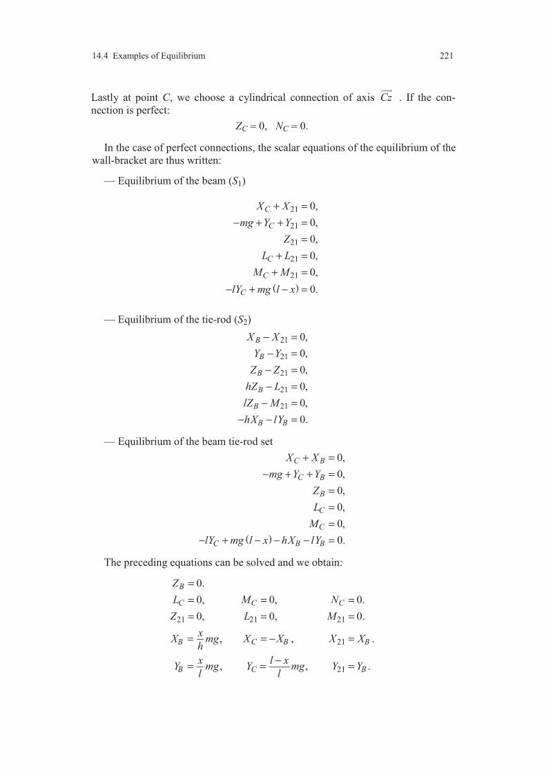
14.4 Examples of Equilibrium 221
Lastly at point C, we choose a cylindrical connection of axis Cz
. If the con-
nection is perfect:
ZC = 0, NC = 0.
In the case of perfect connections, the scalar equations of the equilibrium of the
wall-bracket are thus written:
— Equilibrium of the beam (S1)
( )
21
21
21
21
21
0,
0,
0,
0,
0,
0.
C
C
C
C
C
X X
mg Y Y
Z
L L
M M
lY mg l x
+ =
− + + =
=
+ =
+ =
− + − =
— Equilibrium of the tie-rod (S2)
21
21
21
21
21
0,
0,
0,
0,
0,
0.
B
B
B
B
B
B B
X X
Y Y
Z Z
hZ L
lZ M
hX lY
− =
− =
− =
− =
− =
− − =
— Equilibrium of the beam tie-rod set
( )
0,
0,
0,
0,
0,
0.
C B
C B
B
C
C
C B B
X X
mg Y Y
Z
L
M
lY mg l x hX lY
+ =
− + + =
=
=
=
− + − − − =
The preceding equations can be solved and we obtain:
21 21 21
21
21
0.
0, 0, 0.
0, 0, 0.
, , .
, , .
B
C C C
B C B B
B C B
Z
L M N
Z L M
xX mg X X X X
h
x l xY mg Y mg Y Y
l l
=
= = =
= = =
= = − =
−= = =

222 Chapter 14 Statics of Rigid Bodies
EXERCISES
14.1 Two beams of lengths l1 and l2 are connected between them at point B and
connected to a frame at points A and C (Figure 14.9). The nature of the connection
is to be determined. Two masses m1 and m2 are suspended respectively at the
points M1 and M2 distant of α1l1 and α2l2 from points A and C. The masses of the
beams can be neglected compared to the masses m1 and m2.
14.1.1. Analyze the mechanical actions exerted on each beam.
14.1.2. Derive the equations of equilibrium of the system.
14.1.3. Choose the connections so that the system is isostatic.
14.1.4. The connections being chosen, derive the actions of connections.
14.2 A person (P) climbs up a ladder (S). The ladder is supported on a wall at
point B and rests on the ground at point A (Figure 14.10). To treat of the problem,
it will be supposed that there is a plane symmetry. In particular, the person is such
as it is “located” in the plane of symmetry of the ladder.
The person stands on the ladder, with the feet posed on the rung C and the
hands at point D. The mass centre of the person is at point G.
14.2.1. Analyze the mechanical actions exerted on the person, on the ladder.
14.2.2. Study the equilibrium of the ladder-person set.
FIGURE 14.9. System of two beams.
M1
A
C
1l1
M2
B
2l2
l
hhorizontal

Comments 223
FIGURE 14.10 Equilibrium of a ladder.
COMMENTS
The laws of statics result from the fundamental principle of dynamics
(Chapter 18), and the study of statics should thus be implemented after
having stated the principle of dynamics. However, the analysis of the
equilibrium of sets of rigid bodies allows us to get a good understanding of
the mechanical actions exerted on rigid bodies. The two examples consi-
dered in section 14.4 will be studied with the greatest attention.
B
A
C
D
ground
wall
G


Part IV
Kinetics of Rigid Bodies
The kinematics of rigid bodies considers the motion of bodies without
being concerned with masses to move. However it is easier to move at
a given speed a body of low mass. It is thus necessary to introduce
concepts which associate motion of bodies and mass of bodies. These
concepts are based on the introduction of the notions of kinetic torsor,
dynamic torsor and kinetic energy.

CHAPTER 15
The Operator of Inertia
The concept of operator of inertia, that we study in the present chapter, will
allows us to simply express the different torsors (Chapter 16) necessary to the
study of the dynamics of rigid bodies.
15.1 INTRODUCTION TO THE OPERATOR OF INERTIA
15.1.1 Operator Associated to a Vector Product
Consider two vectors a
and V
, of which the components in the basis (b) =
( ), , i j k
are:
, .x y za a i a j a k V X i Y j Z k= + + = + +
(15.1)
The vector product of the two vectors is written:
( ) ( ) ( )y z z x x ya V a Z a Y i a X a Z j a Y a X k× = − + − + −
. (15.2)
If the vector a
is a given vector, we observe that, whatever the vector V
, the
vector V
is derived from the vector a V×
by a linear operation. Indeed, we have:
( ) ( )
( )
3
31 2 1 2 1 2
and , ,
, , .
V a V a V
V V a V V a V a V
λ λ λ∀ ∈ ∀ ∈ × = ×
∀ ∈ × + = × + ×
(15.3)
It comes to the same thing to say that the vector V
is derived from the vector
a V×
, by making act on V
a linear operator and to write:
.a V V× =
(15.4)
In matrix form, Expression (15.2) of the vector product is written in the
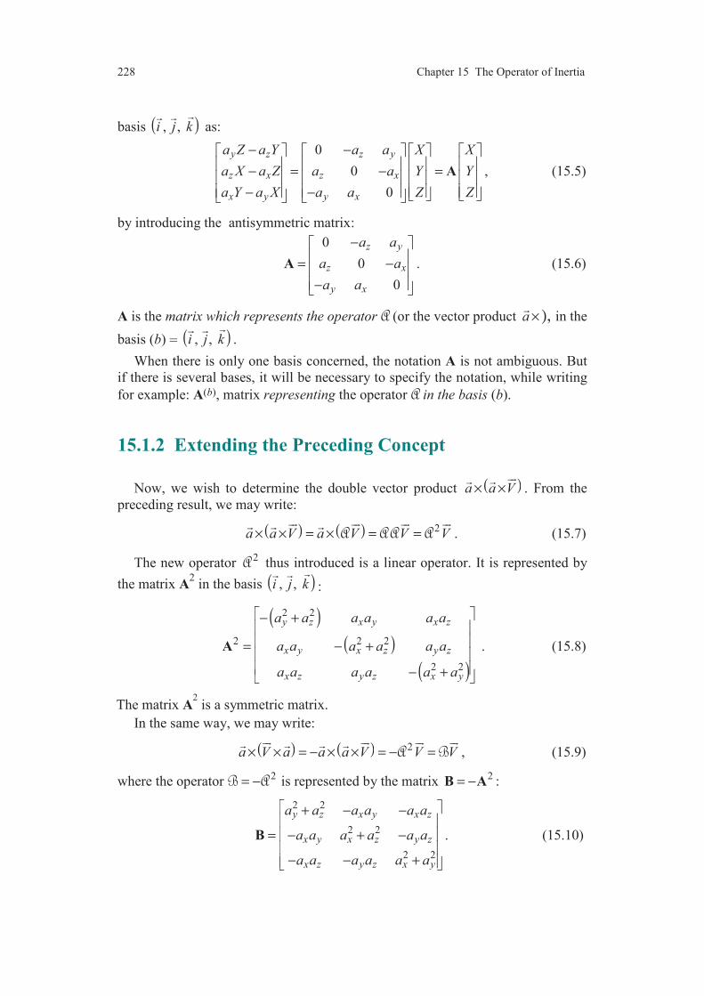
228 Chapter 15 The Operator of Inertia
basis ( ), , i j k
as:
0
0
0
y z z y
z x z x
x y y x
a Z a Y a a X X
a X a Z a a Y Y
a Y a X a a Z Z
− − − = − = − −
A , (15.5)
by introducing the antisymmetric matrix:
0
0
0
z y
z x
y x
a a
a a
a a
− = − −
A . (15.6)
A is the matrix which represents the operator (or the vector product a ×
), in the
basis (b) = ( ), , i j k
.
When there is only one basis concerned, the notation A is not ambiguous. But
if there is several bases, it will be necessary to specify the notation, while writing
for example: A(b), matrix representing the operator in the basis (b).
15.1.2 Extending the Preceding Concept
Now, we wish to determine the double vector product ( )a a V× ×
. From the
preceding result, we may write:
( ) ( ) 2a a V a V V V× × = × = =
. (15.7)
The new operator 2 thus introduced is a linear operator. It is represented by
the matrix A2 in the basis ( ), , i j k
:
( )( )
( )
2 2
2 2 2
2 2
y z x y x z
x y x z y z
x z y z x y
a a a a a a
a a a a a a
a a a a a a
− + = − + − +
A . (15.8)
The matrix A2
is a symmetric matrix.
In the same way, we may write:
( ) ( ) 2a V a a a V V V× × = − × × = − =
, (15.9)
where the operator 2= − is represented by the matrix 2= −B A :
2 2
2 2
2 2
y z x y x z
x y x z y z
x z y z x y
a a a a a a
a a a a a a
a a a a a a
+ − −
= − + −
− − +
B . (15.10)

15.1 Introduction to the Operator of Inertia 229
FIGURE 15.1. Rigid body.
15.1.3 Operator of Inertia
In the evaluation (Chapter 16) of the torsors used in dynamics, we shall have to
express vectors of the form:
( )( )
1 d ( )S
W OM V OM m M= × ×
, (15.11)
( )[ ]( )
2 d ( )S
W OM V V OM m M= × × ×
. (15.12)
The integrals are calculated over the solid (S) (curve, surface or volume). The
point M (Figure 15.1) is a variable point of (S), and d ( )m M is the mass of the
element of (S) surrounding the point M. The point O is a point of reference of the
solid (S). The vector V
is independent of the point M.
From the results derived in the preceding subsection, we may write:
( )1 OW S V= , (15.13)
introducing the operator ( )O S , called operator of inertia at point O of solid (S).
This operator is represented in a basis (b) attached to the solid by a matrix ( )( )bO SI , called matrix of inertia, at point O and in the basis (b), of the solid (S).
The matrix is written according to one of the forms:
( )( )Ox Oxy Oxz
bO Oxy Oy Oyz
Oxz Oyz Oz
A F E I P P
S F B D P I P
E D C P P I
− − − − = − − = − − − − − −
I . (15.14)
If (x, y, z) are the Cartesian coordinates of the point M in the coordinate system ( )/O b = (Oxyz), we have:
y
z
x
O
dm(M)
M
k
(S)
j
i

230 Chapter 15 The Operator of Inertia
OM x i y j z k= + +
, (15.15)
and Expression (15.10) allows us to write:
( )( ) ( )
( )( ) ( )
( )( ) ( )
2 2
2 2
2 2
d ( ), d ( ),
d ( ), d ( ),
d ( ), d ( ).
Ox OxyS S
Oy OxzS S
Oz OyzS S
I y z m M P xy m M
I x z m M P xz m M
I x y m M P yz m M
= + =
= + =
= + =
(15.16)
The quantities IOx, IOy and IOz are called the moments of inertia of the solid (S)
with respect to the axes , , ,Ox Oy Oz
respectively. The quantities POxy, POyz and
POxz are the products of inertia of the solid (S) with respect to the planes (Oxy),
(Oyz) and (Oxz), respectively.
If (X, Y, Z) are the components of the vector V
in the basis (b), the compo-
nents (X1, Y1, Z1) of the vector 1W
in the basis (b) are derived from (15.13) by the
matrix relation: ( )
( )
( )1
1
1
b b
bO
X X
Y Y
Z Z
=
I . (15.17)
Thus:
( ) ( ) ( )1W AX FY EZ i FX BY DZ j EX DY CZ k= − − + − + + + − − +
.
The vector 2W
(15.12) is expressed in the same way in the form:
( )2 OW V S V= ×
(15.18)
Note. ( )O S V
represents the vector derived from the vector V
by making act the
operator ( )O S . The formulation ( )
O S V
must thus be read “the operator ( )O S
acting on V
”. This formulation is comparable with the writing ( ),f x where ( )f x
represents the value obtained from x by the function f.
15.2 CHANGE OF COORDINATE SYSTEM
The change of coordinate reference can be carried out either by change of its
origin or by change of its basis.
15.2.1 Change of Origin
We search for the effect of a change of origin (Figure 15.2). Let (xO', yO', zO')
be the Cartesian coordinates of the new origin O' with respect to the coordinate
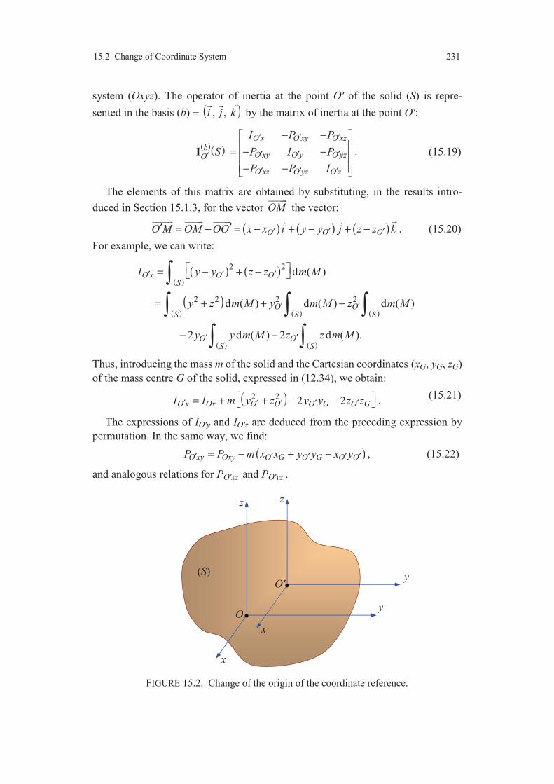
15.2 Change of Coordinate System 231
system (Oxyz). The operator of inertia at the point O' of the solid (S) is repre-
sented in the basis (b) = ( ), , i j k
by the matrix of inertia at the point O':
( )( )O x O xy O xz
bO xy O y O yzO
O xz O yz O z
I P P
S P I P
P P I
′ ′ ′
′ ′ ′′
′ ′ ′
− − = − − − −
I . (15.19)
The elements of this matrix are obtained by substituting, in the results intro-
duced in Section 15.1.3, for the vector OM
the vector:
( ) ( ) ( )O O OO M OM OO x x i y y j z z k′ ′ ′′ ′= − = − + − + −
. (15.20)
For example, we can write:
( ) ( )( )
( )( ) ( ) ( )
( ) ( )
2 2
2 2 2 2
d ( )
d ( ) d ( ) d ( )
2 d ( ) 2 d ( ).
O x O OS
O OS S S
O OS S
I y y z z m M
y z m M y m M z m M
y y m M z z m M
′ ′ ′
′ ′
′ ′
= − + −
= + + +
− −
Thus, introducing the mass m of the solid and the Cartesian coordinates (xG, yG, zG)
of the mass centre G of the solid, expressed in (12.34), we obtain:
( )2 2 2 2O x Ox O O O G O GI I m y z y y z z′ ′ ′ ′ ′ = + + − − . (15.21)
The expressions of IO'y and IO'z are deduced from the preceding expression by
permutation. In the same way, we find:
( )O xy Oxy O G O G O OP P m x x y y x y′ ′ ′ ′ ′= − + − , (15.22)
and analogous relations for PO'xz and PO'yz .
FIGURE 15.2. Change of the origin of the coordinate reference.
y
z
x
O
(S) y
z
x
O'
232 Chapter 15 The Operator of Inertia
15.2.2 Relations of Huyghens
In the case where the point O' coincides with the mass centre G of the solid,
Relations (15.21) and (15.22) are simplified and the matrix of inertia at point G in
the basis (b) may be written in the form:
( )( ) ( )( ) ( ) ( )b b bG O OGS S S= −I I D , (15.23)
with
( ) ( )
( )( )
( )
2 2
2 2
2 2
G G G G G G
bOG G G G G G G
G G G G G G
m y z mx y mx z
S mx y m x z my z
mx z my z m x y
+ − − = − + −
− − +
D . (15.24)
Thus, Expression (15.23) allows us to express the matrix of inertia at O as a
function of the matrix of inertia at G, generally easier to derive:
( )( ) ( )( ) ( ) ( )b b bO G OGS S S= +I I D . (15.25)
This expression leads to the six relations of Huyghens between the moments
and products of inertia:
( )( )( )
2 2
2 2
2 2
, ,
, ,
, .
Ox Gx G G Oxy Gxy G G
Oy Gy G G Oxz Gxz G G
Oz Gz G G Oyz Gyz G G
I I m y z P P mx y
I I m x z P P mx z
I I m x y P P my z
= + + = +
= + + = +
= + + = +
(15.26)
15.2.3 Diagonalisation of the Matrix of Inertia
We deduce from the properties of the symmetric linear operators the following
fundamental results.
The operator of inertia ( )O S has at least an orthonormal basis of eigen vectors
( )1 2 3, , u u u
called the principal basis at point O.
The axes ( ), iO u
are called principal axes of inertia at the point O, and the
reference ( )1 2 3/ , , O u u u
is the principal reference of inertia at the point O.
In the basis ( )1 2 3, , u u u
, the matrix of inertia at the point O is a diagonal
matrix, called principal matrix of inertia at the point O. Its non-zero terms are the
principal moments of inertia at the point O.
In the principal basis (p), the matrix is thus written as:
( )( )1
2
3
0 0
0 0
0 0
pO
I
S I
I
=
I , (15.27)
where I1, I2 et I3 are the principal moments of inertia at the point O. We deduce:
15.2 Change of Coordinate System 233
( ) ( ) ( ) 1 1 1 2 2 2 3 3 3, , .O O OS u I u S u I u S u I u= = =
(15.28)
The principal moments of inertia Ii (i = 1, 2, 3) can thus be obtained by expressing
Relations (15.28) in the form:
( )O i i iS u I u=
. (15.29)
In the non principal basis (b), this relation is written:
i i
i i i
i i
A F E u u
F B D v I v
E D C w w
− − − − = − −
, (15.30)
by introducing the components (ui, vi , wi ) in the basis (b) of the eigen vector iu
.
The preceding expression can be rewritten:
0
0
0
i i
i i
i i
A I F E u
F B I D v
E D C I w
− − − − − − = − − −
. (15.31)
The vectors iu
being different from the null vector, this system has solutions if
the determinant is zero:
det 0
i
i
i
A I F E
F B I D
E D C I
− − − − − − = − − −
. (15.32)
This equation allows us to obtain the principal moments I1, I2 and I3. The principal
directions are then determined by substituting I1, I2 and I3 into Relation (15.30).
15.2.4 Change of Basis
Let ( ) ( )1 1 1 1, , b i j k=
and ( ) ( )2 2 2 2, , b i j k=
be two bases related by the basis
change:
2 1
2 1
2 1
i i
j j
k k
=
A
, (15.33)
where A is the matrix of basis change. The expressions of the matrices of inertia
allow us to establish the relation which expresses the matrix of inertia ( )( )2bO SI at
the point O in the basis (b2) as a function of the matrix of inertia in the basis (b1).
This relation is written in the form: ( )( ) ( )( )2 1 tb bO OS S=I A I A , (15.34)
where At is the matrix transposed of the matrix A.

234 Chapter 15 The Operator of Inertia
15.3 MOMENTS OF INERTIA WITH RESPECT TO
A POINT, AN AXIS, A PLANE
15.3.1 Definitions
We call moment of inertia of a solid (S) with respect to a point (with respect to
an axis or with respect to a plane) the integral:
( )
2d ( ),S
l m M (15.35)
where l is the distance (for example Figure 15.3) from the variable point M of the
solid (S) to the point under consideration (to the axis or to the plane).
If (x, y, z) are the coordinates of point M relatively to a system of origin O, the
expressions of the moments of inertia of the solid (S) are from (15.35):
1. Moment of inertia with respect to the point O:
( ) ( )( )
2 2 2 d ( )OS
I S x y z m M= + + . (15.36)
2. Moments of inertia with respect to the axes , , ,Ox Oy Oz
(already expressed
in 15.16):
( )( )
( )( )
( )( )
2 2
2 2
2 2
d ( ),
d ( ),
d ( ).
OxS
OyS
OzS
I y z m M
I x z m M
I x y m M
= +
= +
= +
(15.37)
FIGURE 15.3. Distances from an arbitrary point to a point, an axis, a plane.
y
z
x
O
M
l
y
z
x
O
M
l
y
z
x
O
M
l
15.3 Moments of Inertia with respect to a Point, an Axis, a Plane 235
3. Moments of inertia with respect to the planes (Oxy), (Oyz), (Oxz):
( )
( )
( )
2
2
2
d ( ),
d ( ),
d ( ).
OxyS
OyzS
OxzS
I z m M
I x m M
I y m M
=
=
=
(15.38)
15.3.2 Relations between the Moments of Inertia
By addition of the integrals (15.36) to (15.38), we obtain the following pro-
perties:
1. The sum of the moments of inertia of a solid with respect to three trirect-
angular axes intersecting at a same point is equal to twice the moment of inertia of
the solid with respect to this point:
2Ox Oy Oz OI I I I+ + = . (15.39)
2. The sum of the moments of inertia of a solid with respect to two perpen-
dicular planes is equal to the moment of inertia of the solid with respect to the axis
intersection of these two planes:
,
,
.
Oxy Oxz Ox
Oxy Oyz Oy
Oxz Oyz Oz
I I I
I I I
I I I
+ =
+ =
+ =
(15.40)
15.3.3 Case of a Plane Solid
In the case of a plane solid, contained in the plane (Oxy) (Figure 15.4), point M
of the solid has for coordinates (x, y, 0) and the moments of inertia are reduced to:
( )( )
( )
( )
( )( )
2 2
2
2
2 2
d ( ),
d ( ),
d ( ),
d ( ).
OS
OxS
OyS
OzS
I x y m M
I y m M
I x m M
I x y m M
= +
=
=
= +
(15.41)
Between the moments of inertia, we have the relation:
Oz O Ox OyI I I I= = + . (15.42)

236 Chapter 15 The Operator of Inertia
FIGURE 15.4. Plane solid.
15.3.4 Moment of Inertia with Respect to an Arbitrary Axis
Let us express the moment of inertia of solid (S) with respect to the axis (∆) of
unit direction vector u
and passing through the point O (Figure 15.5). Hence from
(15.35):
( )
2d ( )S
I HM m M∆ = , (15.43)
where H is the orthogonal projection of point M on the axis (∆). We have then:
HM u OM= ×
. (15.44)
Hence:
( ) ( ) ( )22 22HM z y x z y xβ γ γ α α β= − + − + − , (15.45)
introducing the components (α, β, γ) of the vector u
and the coordinates (x, y, z)
of point M. The components (α, β, γ) of the unit direction vector of the axis (∆)
FIGURE 15.5. Moment of inertia with respect to an arbitrary axis.
y
z
x
OM
(S)
y
z
x
O
(S)
()
M
15.4 Determination of Matrices of Inertia 237
are also called the direction cosines of the axis. Reporting Relation (15.45) into
Expression (15.43), we obtain:
2 2 2 2 2 2Ox Oy Oz Oxy Oyz OxzI I I I P P P∆ α β γ αβ βγ αγ= + + − − − . (15.46)
This relation can also be expressed, introducing the operator of inertia at the
point O, in the form: ( )
OI u S u∆ = ⋅ , (15.47)
or in the matrix form:
[ ]Ox Oxy Oxz
Oxy Oy Oyz
Oxz Oyz Oz
I P P
I P I P
P P I
∆
α
α β γ β
γ
− − = − − − −
. (15.48)
In the case where the operator of inertia is referred to its principal axes, Rela-
tion (15.46) is reduced to: 2 2 21 1 2 2 3 3I I I I∆ α α α= + + , (15.49)
where (α1, α2, α3) are the direction cosines of the axis (∆) with respect to the prin-
cipal axes at point O.
15.4 DETERMINATION OF MATRICES OF INERTIA
15.4.1 Solids with Material Symmetries
In the case where the solids have material symmetries, these symmetries make
easier the research of the principal axes of inertia. From this it results a simpli-
fication for deriving the matrix of inertia.
15.4.1.1 Plane of Symmetry
Suppose that the solid (S) has a plane of material symmetry, for example the
plane (Oxy) (Figure 15.6a). It results that the products of inertia:
( )( )
d ( ) and d ( )Oxz OyzS S
P xz m M P yz m M= = are zero, since it is possible to associate elements which have the same value of x
(or of y) and opposite values of z (Figure 15.6a). Thus, we have:
0 0 0 0
0 0 0 0
0 0 1 1
Ox Oxy
Oxy Oy Oz
Oz Oz
I P
P I I
I I
− − = =
, (15.50)
or
( )O OzS k I k=
. (15.51)
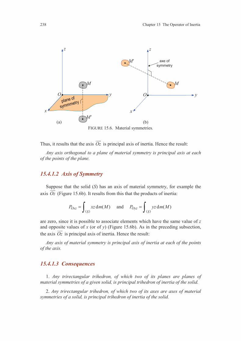
238 Chapter 15 The Operator of Inertia
FIGURE 15.6. Material symmetries.
Thus, it results that the axis Oz
is principal axis of inertia. Hence the result:
Any axis orthogonal to a plane of material symmetry is principal axis at each
of the points of the plane.
15.4.1.2 Axis of Symmetry
Suppose that the solid (S) has an axis of material symmetry, for example the
axis Oz
(Figure 15.6b). It results from this that the products of inertia:
( )( )
d ( ) and d ( )Oxz OyzS S
P xz m M P yz m M= = are zero, since it is possible to associate elements which have the same value of z
and opposite values of x (or of y) (Figure 15.6b). As in the preceding subsection,
the axis Oz
is principal axis of inertia. Hence the result:
Any axis of material symmetry is principal axis of inertia at each of the points
of the axis.
15.4.1.3 Consequences
1. Any trirectangular trihedron, of which two of its planes are planes of
material symmetries of a given solid, is principal trihedron of inertia of the solid.
2. Any trirectangular trihedron, of which two of its axes are axes of material
symmetries of a solid, is principal trihedron of inertia of the solid.
axe of
symmetry
y
z
x
O
M
M'
(b)
(a)
y
z
x
O
M
M'(a)
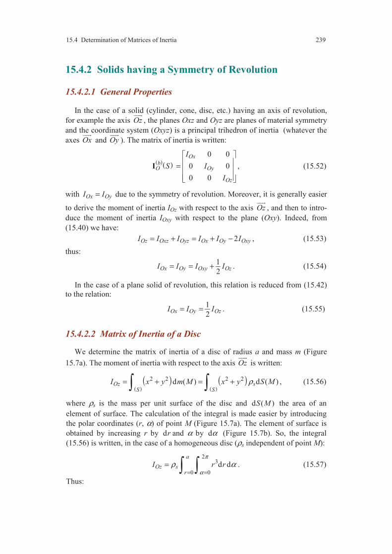
15.4 Determination of Matrices of Inertia 239
15.4.2 Solids having a Symmetry of Revolution
15.4.2.1 General Properties
In the case of a solid (cylinder, cone, disc, etc.) having an axis of revolution,
for example the axis Oz
, the planes Oxz and Oyz are planes of material symmetry
and the coordinate system (Oxyz) is a principal trihedron of inertia (whatever the
axes Ox
and Oy
). The matrix of inertia is written:
( )( )
0 0
0 0
0 0
Oxb
O Oy
Oz
I
S I
I
=
I , (15.52)
with Ox OyI I= due to the symmetry of revolution. Moreover, it is generally easier
to derive the moment of inertia IOz with respect to the axis Oz
, and then to intro-
duce the moment of inertia IOxy with respect to the plane (Oxy). Indeed, from
(15.40) we have:
2Oz Oxz Oyz Ox Oy OxyI I I I I I= + = + − , (15.53)
thus:
1
2Ox Oy Oxy OzI I I I= = + . (15.54)
In the case of a plane solid of revolution, this relation is reduced from (15.42)
to the relation:
1
2Ox Oy OzI I I= = . (15.55)
15.4.2.2 Matrix of Inertia of a Disc
We determine the matrix of inertia of a disc of radius a and mass m (Figure
15.7a). The moment of inertia with respect to the axis Oz
is written:
( )( )
( )( )
2 2 2 2d ( ) d ( )Oz sS S
I x y m M x y S Mρ= + = + , (15.56)
where ρs is the mass per unit surface of the disc and d ( )S M the area of an
element of surface. The calculation of the integral is made easier by introducing
the polar coordinates (r, α) of point M (Figure 15.7a). The element of surface is
obtained by increasing r by dr and α by dα (Figure 15.7b). So, the integral
(15.56) is written, in the case of a homogeneous disc (ρs independent of point M):
23
0 0
d da
Oz sr
I r rπ
αρ α
= == . (15.57)
Thus:
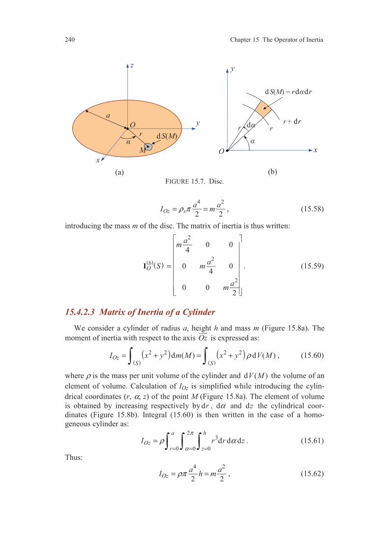
240 Chapter 15 The Operator of Inertia
FIGURE 15.7. Disc.
4 2
2 2Oz s
a aI mρ π= = , (15.58)
introducing the mass m of the disc. The matrix of inertia is thus written:
( )( )
2
2
2
0 04
0 04
0 02
bO
am
aS m
am
=
I . (15.59)
15.4.2.3 Matrix of Inertia of a Cylinder
We consider a cylinder of radius a, height h and mass m (Figure 15.8a). The
moment of inertia with respect to the axis Oz
is expressed as:
( )( )
( )( )
2 2 2 2d ( ) d ( )OzS S
I x y m M x y V Mρ= + = + , (15.60)
where ρ is the mass per unit volume of the cylinder and d ( )V M the volume of an
element of volume. Calculation of IOz is simplified while introducing the cylin-
drical coordinates (r, α, z) of the point M (Figure 15.8a). The element of volume
is obtained by increasing respectively by dr , dα and dz the cylindrical coor-
dinates (Figure 15.8b). Integral (15.60) is then written in the case of a homo-
geneous cylinder as:
23
0 0 0
d d da h
Ozr z
I r r zπ
αρ α
= = == . (15.61)
Thus: 4 2
2 2Oz
a aI h mρπ= = , (15.62)
(b)
y
z
x
O
M
d S(M)
a
(a)
r
x
y
O
d
d S(M) = rddr
r rr + dr

15.4 Determination of Matrices of Inertia 241
dr
FIGURE 15.8. Cylinder.
introducing the mass m of the cylinder.
The moment of inertia with respect to the plane Oxy is written:
2 22
0 0 0
d d d3
a h
Oxyr z
hI z r r z m
π
αρ α
= = == = . (15.63)
We then deduce, from (15.54):
2 2
4 3Ox Oy
a hI I m
= = +
. (15.64)
15.4.3 Solid with a Spherical Symmetry
15.4.3.1 General Properties
In the case of a body with spherical symmetry (solid sphere, hollow sphere,
etc.) of centre O, any system (Oxyz) is principal trihedron of inertia, and the
moments of inertia with respect to the axes are equal. It is then more convenient to
calculate the moment of inertia IO with respect to the point O and to express the
moments by taking account of Relation (15.39). Thus:
2
3Ox Oy Oz OI I I I= = = . (15.65)
15.4.3.2 Matrix of Inertia of a Solid Sphere
We have to determine the matrix of inertia of a solid sphere of mass m and
radius a (Figure 15.9a). The calculation of the moment of inertia with respect to
(a)
y
z
x
O
r
Mz
(b)
x
yO
d
d V(M) = rddrdz
z
r
dr
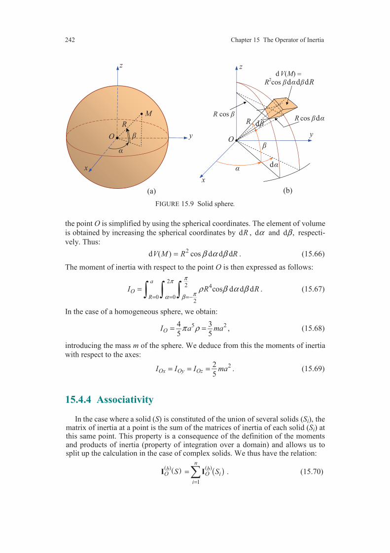
242 Chapter 15 The Operator of Inertia
FIGURE 15.9 Solid sphere.
the point O is simplified by using the spherical coordinates. The element of volume
is obtained by increasing the spherical coordinates by dR , dα and d ,β respecti-
vely. Thus:
2d ( ) cos d d dV M R Rβ α β= . (15.66)
The moment of inertia with respect to the point O is then expressed as follows:
22 4
0 02
cos d d da
OR
I R R
ππ
πα βρ β α β
= = =−= . (15.67)
In the case of a homogeneous sphere, we obtain:
5 24 3
5 5OI a maπ ρ= = , (15.68)
introducing the mass m of the sphere. We deduce from this the moments of inertia
with respect to the axes:
22
5Ox Oy OzI I I ma= = = . (15.69)
15.4.4 Associativity
In the case where a solid (S) is constituted of the union of several solids (Si), the matrix of inertia at a point is the sum of the matrices of inertia of each solid (Si) at this same point. This property is a consequence of the definition of the moments and products of inertia (property of integration over a domain) and allows us to split up the calculation in the case of complex solids. We thus have the relation:
( )( ) ( )( )1
nb b
O O i
i
S S
=
=I I . (15.70)
(a) (b)
z
y
M
O
R
x
x
yO
d
d V(M) = R
2cos dddR
z
R
d
R cos R cos d
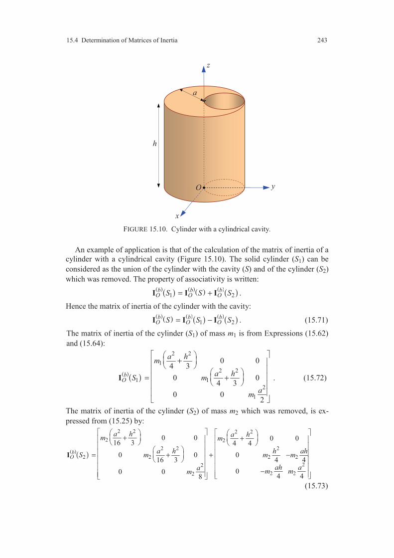
15.4 Determination of Matrices of Inertia 243
FIGURE 15.10. Cylinder with a cylindrical cavity.
An example of application is that of the calculation of the matrix of inertia of a
cylinder with a cylindrical cavity (Figure 15.10). The solid cylinder (S1) can be
considered as the union of the cylinder with the cavity (S) and of the cylinder (S2)
which was removed. The property of associativity is written:
( )( ) ( )( ) ( )( )1 2b b b
O O OS S S= +I I I .
Hence the matrix of inertia of the cylinder with the cavity:
( )( ) ( )( ) ( )( )1 2b b b
O O OS S S= −I I I . (15.71)
The matrix of inertia of the cylinder (S1) of mass m1 is from Expressions (15.62)
and (15.64):
( )( )
2 2
1
2 2
1 1
2
1
0 04 3
0 04 3
0 02
bO
a hm
a hS m
am
+
= +
I . (15.72)
The matrix of inertia of the cylinder (S2) of mass m2 which was removed, is ex-
pressed from (15.25) by:
( )( )
2 2 2 2
2 2
2 2 2
2 2 2 2
22
2 22
0 0 0 016 3 4 4
0 0 016 3 4 4
00 04 48
bO
a h a hm m
a h h ahS m m m
ah aam mm
+ + = + + −
−
I
(15.73)
h
a
O
x
y
z

244 Chapter 15 The Operator of Inertia
In addition, the masses of the cylinders are related to the mass m of the cylinder
hollowed out by the relations:
1 24
, 5 5
mm m m= = . (15.74)
Hence the matrix of the cylinder with the cavity:
( )( )
( )( )
2 2
2 2
2
113 0 0
20 4
150 3
20 4 20
020 4
bO
ma h
m mS a h ah
m aah m
+ = +
I . (15.75)
15.5 MATRICES OF INERTIA OF HOMOGENEOUS
BODIES
We collect in this section the matrices of inertia of various homogeneous solids.
The matrices of inertia are referred to the basis (b) = ( ), , i j k
associated for each
solid to the coordinate system chosen, generally the principal system of inertia.
15.5.1 One-Dimensional Solids
15.5.1.1 Straight Rod (Figure 15.11)
The length of the segment of line is AB = l. The mass centre is given by:
2
lAG i=
.
The matrix of inertia at the point A is:
( )( )2
2
0 0 0
0 03
0 03
bA
lS m
lm
=
I . (15.76)
FIGURE 15.11. Straight rod.
z
A BG
y
x

15.5 Matrices of Inertia of Homogeneous Bodies 245
FIGURE 15.12. Arc of circle.
15.5.1.2 Arc of Circle (Figure 15.12)
The arc of circle is characterized by its radius a and its angle 2α. The position
of the mass centre and the matrix of inertia are expressed by:
sinOG a i
αα
=
, (15.77)
( )( )
( )( )
2
2
2
sin 21 0 0
2 2
sin 20 1 0
2 2
0 0
bO
am
aS m
ma
αα
αα
−
= +
I . (15.78)
Particular cases
— Semicircle: 2
πα =
( )( )
2
2
2
0 02
2, 0 0
2
0 0
bO
am
a aOG i S m
ma
π
= =
I
. (15.79)
— Circle (case of a hoop): α π=The mass centre is at the point O and the matrix of inertia at O has the same
form as the semicircle.
15.5.2 Two-Dimensional Solids
15.5.2.1 Circular Sector (Figure 15.13)
As arc of circle, the circular sector is characterized by its radius and its angle
2α. The position of the mass centre and the matrix of inertia are expressed by:
a
x G
z
y
−O
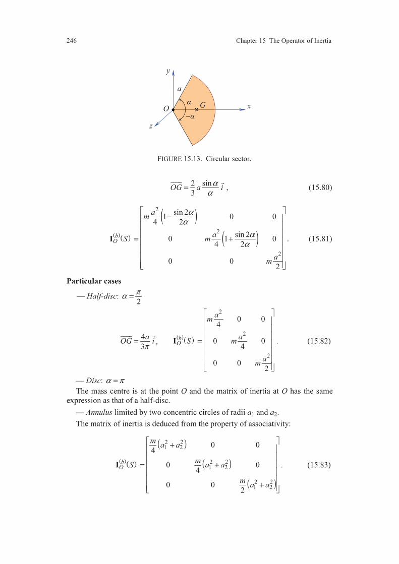
246 Chapter 15 The Operator of Inertia
FIGURE 15.13. Circular sector.
2 sin
3OG a i
αα
=
, (15.80)
( )( )
( )( )
2
2
2
sin 21 0 0
4 2
sin 20 1 0
4 2
0 02
bO
am
aS m
am
αα
αα
−
= +
I . (15.81)
Particular cases
— Half-disc: 2
πα =
( )( )
2
2
2
0 04
4, 0 0
3 4
0 02
bO
am
a aOG i S m
am
π
= =
I
. (15.82)
— Disc: α π=
The mass centre is at the point O and the matrix of inertia at O has the same
expression as that of a half-disc.
— Annulus limited by two concentric circles of radii a1 and a2.
The matrix of inertia is deduced from the property of associativity:
( )( )
( )
( )
( )
2 21 2
2 21 2
2 21 2
0 04
0 04
0 02
bO
ma a
mS a a
ma a
+ = +
+
I . (15.83)
a
G
−
x
y
z
O
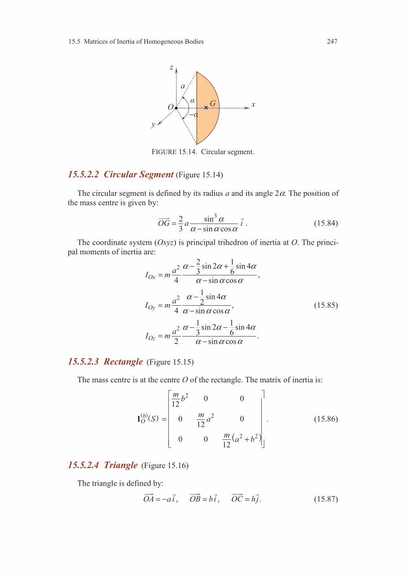
15.5 Matrices of Inertia of Homogeneous Bodies 247
FIGURE 15.14. Circular segment.
15.5.2.2 Circular Segment (Figure 15.14)
The circular segment is defined by its radius a and its angle 2α. The position of
the mass centre is given by:
32 sin
3 sin cosOG a i
αα α α
=−
. (15.84)
The coordinate system (Oxyz) is principal trihedron of inertia at O. The princi-
pal moments of inertia are:
2
2
2
2 1sin 2 sin 4
3 6 ,4 sin cos
1sin 4
2 ,4 sin cos
1 1sin 2 sin 4
3 6 .2 sin cos
Ox
Oy
Oz
aI m
aI m
aI m
α α α
α α α
α α
α α α
α α α
α α α
− +=
−
−=
−
− −=
−
(15.85)
15.5.2.3 Rectangle (Figure 15.15)
The mass centre is at the centre O of the rectangle. The matrix of inertia is:
( )( )
( )
2
2
2 2
0 012
0 012
0 012
bO
mb
mS a
ma b
=
+
I . (15.86)
15.5.2.4 Triangle (Figure 15.16)
The triangle is defined by:
, , .OA a i OB bi OC hj= − = =
(15.87)
a
G
−x
y
z
O

248 Chapter 15 The Operator of Inertia
FIGURE 15.15. Rectangle.
The position of the mass centre is given by:
3 3
b a hOG i j
−= +
. (15.88)
The matrices of inertia at the point O and at the mass centre are expressed as:
( )( )
( )
( ) ( )
( )
2
2 2
2 2 2
06 12
012 6
0 06
bO
m mh h b a
m mS h b a a ab b
ma ab b h
− − = − − − +
− + +
I , (15.89)
( )( )
( )
( ) ( )
( )
2
2 2
2 2 2
018 36
036 18
0 018
bG
m mh h b a
m mS h b a a ab b
ma ab b h
− = − + +
+ + +
I . (15.90)
FIGURE 15.16. Triangle.
x
a
y
z
O b
A x
y
z
O B
C
G
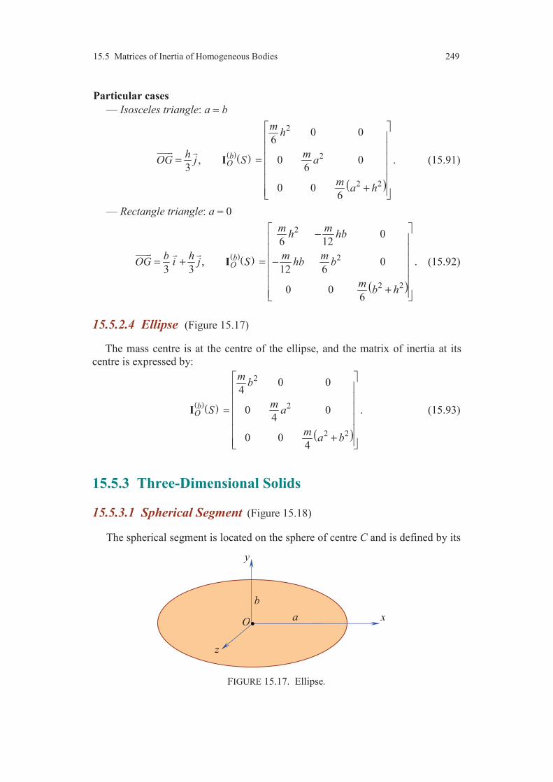
15.5 Matrices of Inertia of Homogeneous Bodies 249
Particular cases— Isosceles triangle: a = b
( )( )
( )
2
2
2 2
0 06
, 0 03 6
0 06
bO
mh
h mOG j S a
ma h
= =
+
I
. (15.91)
— Rectangle triangle: a = 0
( )( )
( )
2
2
2 2
06 12
, 03 3 12 6
0 06
bO
m mh hb
b h m mOG i j S hb b
mb h
− = + = −
+
I
. (15.92)
15.5.2.4 Ellipse (Figure 15.17)
The mass centre is at the centre of the ellipse, and the matrix of inertia at its
centre is expressed by:
( )( )
( )
2
2
2 2
0 04
0 04
0 04
bO
mb
mS a
ma b
=
+
I . (15.93)
15.5.3 Three-Dimensional Solids
15.5.3.1 Spherical Segment (Figure 15.18)
The spherical segment is located on the sphere of centre C and is defined by its
FIGURE 15.17. Ellipse.
x
y
z
O a
b

250 Chapter 15 The Operator of Inertia
FIGURE 15.18. Spherical segment.
height h and the radius a of the sphere. Its volume is:
( )2 33
V h a hπ
= − , (15.94)
and its mass centre is defined by:
( )23 2
4 3
a hCG a k
a h
−=
−
. (15.95)
The system (Oxyz) is principal trihedron of inertia and the moments of inertia are:
( )
22
2 2
,3 4 20
2 3 3.
3 4 20
Ox Oy
Oz
m h ah hI I a
a h
hI m a ah h
a h
= = − +
−
= − +−
(15.96)
Particular cases
— Half-sphere
The points C and O coincide and the radius of the circle of the base is the
radius of the half-sphere.
23 2, .
8 5Ox Oy OzOG a k I I I ma= = = =
(15.97)
— Sphere
The matrix of inertia was derived in Subsection 15.4.3.2. Its expression is the
same as that of the half-sphere.
15.5.3.2 Circular Cone (Figure 15.19)
The cone is defined by its height h and the radius a of the circle of the base.
The mass centre and the matrix of inertia are given by:
3
4OG hk=
. (15.98)
h
a
z
G
y
x
O
C
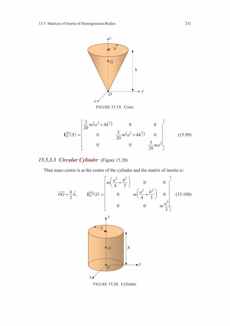
15.5 Matrices of Inertia of Homogeneous Bodies 251
FIGURE 15.19. Cone.
( )( )
( )
( )
2 2
2 2
2
34 0 0
203
0 4 020
30 0
20
bO
m a h
S m a h
ma
+
= +
I . (15.99)
15.5.3.3 Circular Cylinder (Figure 15.20)
Thee mass centre is at the centre of the cylinder and the matrix of inertia is:
( )( )
2 2
2 2
2
0 04 3
, 0 02 4 3
0 02
bO
a hm
h a hOG k S m
am
+
= = +
I
(15.100)
FIGURE 15.20. Cylinder.
h
a
y
x
z
O
G
h
y
x
z
O
a
G

252 Chapter 15 The Operator of Inertia
15.5.3.4 Rectangle Parallelepiped (Figure 15.21)
The mass centre is at the centre of the parallelepiped:
2 2 2
a b cOG i j k= + +
, (15.101)
and the matrix of inertia at the mass centre is:
( )( )
( )
( )
( )
2 2
2 2
2 2
0 012
0 012
0 012
bG
mb c
mS a c
ma b
+ = +
+
I . (15.102)
The matrix of inertia at the point O, one of the vertices of the parallelepiped, is
deduced from the matrix at the centre by applying the relations of Huyghens. We
obtain:
( )( )
( )
( )
( )
2 2
2 2
2 2
3 4 4
4 3 4
4 4 3
bO
m m mb c ab ac
m m mS ab a c bc
m m mac bc a b
+ − − = − + −
− − +
I . (15.103)
FIGURE 15.21 Rectangle parallelepiped.
c
y
x
z
O
G
a
b

Exercises 253
EXERCISES
15.1 Derive the principal matrix of inertia at the centre of a rectangular plate of
low thickness (Figure 15.22). Next, deduce the moment of inertia with respect to
an axis (∆) contained in the plane of the plate and forming an angle θ with the axis
Ox
.
15.2 Express the matrix of inertia of a quarter of disc. Study the variation of the
moment of inertia with respect to an axis contained in the plane of the disc.
15.3 Derive the matrix of inertia of a homogeneous hollowed cylinder, of inner
radius a1, of outer radius a2 and of height h.
15.4 Derive the matrix of inertia of a solid (Figure 15.24) constituted of a cylin-
der of height h and of a solid half-sphere of radius a.
FIGURE 15.22. Rectangular plate.
FIGURE 15.23. Association of a cylinder
and a solid half-sphere.
y
x
a
b O
()
(S1)
z
h
a
O
(S2)
y
x
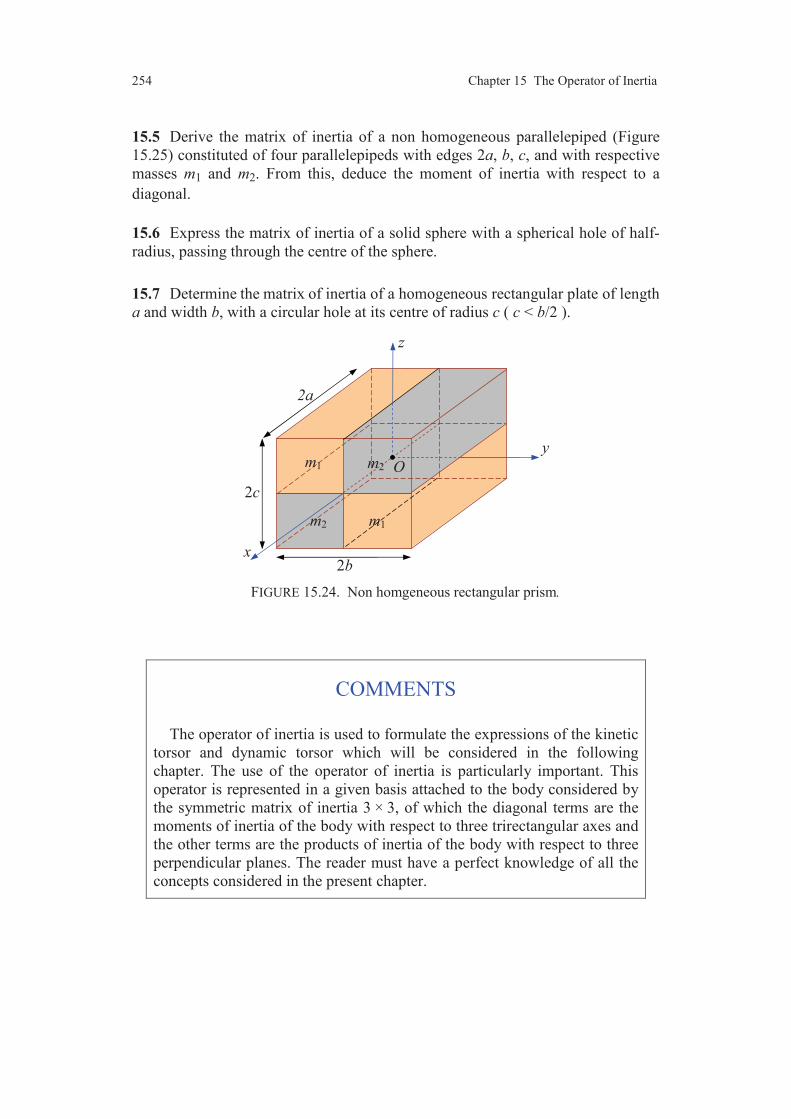
254 Chapter 15 The Operator of Inertia
15.5 Derive the matrix of inertia of a non homogeneous parallelepiped (Figure
15.25) constituted of four parallelepipeds with edges 2a, b, c, and with respective
masses m1 and m2. From this, deduce the moment of inertia with respect to a
diagonal.
15.6 Express the matrix of inertia of a solid sphere with a spherical hole of half-
radius, passing through the centre of the sphere.
15.7 Determine the matrix of inertia of a homogeneous rectangular plate of length
a and width b, with a circular hole at its centre of radius c ( c < b/2 ).
FIGURE 15.24. Non homgeneous rectangular prism.
COMMENTS
The operator of inertia is used to formulate the expressions of the kinetic
torsor and dynamic torsor which will be considered in the following
chapter. The use of the operator of inertia is particularly important. This
operator is represented in a given basis attached to the body considered by
the symmetric matrix of inertia 3 × 3, of which the diagonal terms are the
moments of inertia of the body with respect to three trirectangular axes and
the other terms are the products of inertia of the body with respect to three
perpendicular planes. The reader must have a perfect knowledge of all the
concepts considered in the present chapter.
2c
y
x
z
2a
2b
Om1
m1 m2
m2

CHAPTER 16
Kinetic and Dynamic Torsors Kinetic Energy
16.1 KINETIC TORSOR
16.1.1 Definition
The study of dynamics introduced a first torsor which allows us to express the
kinetic energy (Section 16.3) and whose concept is also used within the frame of
the theory of impacts. This torsor called kinetic torsor, denoted by ( ) T
D and
associated to the motion of a material set (D) relatively to a reference (T), is
defined over the set (D) in the following way.
We call kinetic torsor relative to the motion of the material set (D) with respect
to the reference (T), the torsor defined on this set and associated to the field of
sliders of which the vector density (relative to the mass) in every point of the
material set (D) is equal to the velocity vector of this point with respect to the
reference (T).
The kinetic torsor ( ) T
D is thus associated to the field of sliders (Section
5.3.2.) of resultants:
( )M D∀ ∈ ( )
d ( ) ( , ) d ( )TR M M t m M=
. (16.1)
From (5.54) and (5.55), the elements of reduction of the kinetic torsor at a
point P of the reference (T) are:
( ) ( )
( )( , ) d ( )T T
DD
R M t m M= , (16.2)
( ) ( )
( )( , ) d ( )T T
P DD
PM M t m M= × . (16.3)

256 Chapter 16 Kinetic and Dynamic Torsors. Kinetic Energy
FIGURE 16.1. Motion of the set (D) relatively to a given reference.
16.1.2 Kinetic Torsor Associated to the Motion of a Body
Consider a solid (S) in motion relatively to the reference (T). This motion is
characterized (Chapter 9) by the motion of a particular point P of the solid (S) (or
attached to the solid) and by its rotation vector ( )TSω
. We established (9.11):
( ) ( ) ( ) ( , ) ( , )T T T
SM t P t PMω= + ×
.
The elements of reduction of the kinetic torsor at the point P of the solid (S) are
derived by substituting this expression into Relations (16.2) and (16.3).
1. Resultant of the kinetic torsor
Relation (16.2) is written:
( ) ( ) ( )
( ) ( , ) d ( )T T T
S SS
R P t PM m Mω = + × .
Hence:
( ) ( )
( )
( )
( )
( , ) d ( ) d ( )T T TS S
S S
R P t m M PM m Mω= + × .
Thus, by introducing the mass centre and the mass of the solid (Relation (12.23)),
we obtain:
( ) ( ) ( )( , )T T T
S SR m P t PGω = + × . (16.4)
Or:
( ) ( )( , )T T
SR m G t= . (16.5)
Hence the result:
The resultant of the kinetic torsor associated to the motion of a solid relatively
to a given reference is equal to the product of the mass of the solid by the velocity
vector, in this reference, of the mass centre of the solid.
y
z
x
O
(T) dm(M)
M (D)
P
16.1 Kinetic Torsor 257
2. Moment vector of the kinetic torsor
Relation (16.3) is written:
( )
( )
( ) ( )( )( )
d ( ) ( , ) d ( )T T TP S S
S S
PM m M P t PM PM m Mω
= × + × ×
.
The mass centre can be introduced in the first integral. The second integral is
expressed by introducing the operator of inertia at point P of the body (S). The
moment vector at the point P is thus written in the form:
( ) ( ) ( ) ( ) ( , )T T T
P S P Sm PG P t S ω= × + . (16.6)
This expression is simplified, when the moment-vector is expressed at the mass
centre (P coincides with G):
( ) ( ) ( )T TG S G SS ω=
. (16.7)
This simplification confirms the importance of the concept of the mass centre.
16.1.3 Kinetic Torsor for a Set of Bodies
We call kinetic torsor associated to the motion, relatively to a given reference,
of a set (D), constituted of solids ( ) ( ) ( ) 1 2, , . . . , ,nS S S the torsor obtained by
doing the sum of the kinetic torsors associated to the motions of every solid
relatively to the reference under consideration.
We thus have the relation:
( ) ( ) 1
i
nT T
D S
i=
= . (16.8)
This relation leads to the expressions of the elements of reduction of the kinetic
torsor:
( ) ( ) ( )
1 1
( , )i
n nT T T
D i iS
i i
R R m G t
= =
= = .
Thus:
( ) ( )( , )T T
DR m G t= , (16.9)
where m and G are respectively the mass and the mass centre of the set (D). We
find again the same expression of the resultant as in the case of only one solid
(Relation (16.5)). The moment vector at a point P of reference is written in the
form:
( ) ( ) ( ) ( ) ( )1 1
ii i i
n nT T T T
P P GD iS S S
i i
R G P
= =
= = + ×
,

258 Chapter 16 Kinetic and Dynamic Torsors. Kinetic Energy
or introducing Relations (16.5) and (16.7) for every solid:
( ) ( ) ( ) ( )
1
( , )i i
nT T T
P D i i i G i S
i
m PG G t S ω=
= × + . (16.10)
16.2 DYNAMIC TORSOR
16.2.1 Definition
The fundamental principle of the dynamics (Chapter 18) utilizes the dynamic
torsor, denoted by ( ) T
D and defined over the material set as follows.
We call dynamic torsor relative to the motion of the material set (D) with
respect to the reference (T), the torsor defined over this set and associated to the
field of sliders of which the vector density (relative to the mass) in every point of
the material set (D) is equal to the acceleration vector of this point with respect to
the reference (T).
The dynamic torsor ( ) T
D is thus associated to the field of sliders of resul-
tants:
( )M D∀ ∈ ( )
d ( ) ( , ) d ( )TR M a M t m M=
. (16.11)
From (5.54) and (5.55), the elements of reduction at a point P of the dynamic
torsor are:
( ) ( )
( )( , ) d ( )T T
DD
R a M t m M= , (16.12)
( ) ( )
( )( , ) d ( )T T
P DD
PM a M t m M= × . (16.13)
16.2.2 Dynamic Torsor Associated to the Motion of a Body
Consider a solid (S) in motion relatively to the reference (T). We established
(9.24): ( ) ( ) ( ) ( ) ( )( ) ( , ) ( , )T T T T T
S S Sa M t a P t PM PMω ω ω= + × + × × .
The elements of reduction at a particular point P of the solid (S) are derived
while substituting this expression into Relations (16.12) and (16.13).
1. Resultant of the dynamic torsor
Relation (16.12) is written:
( ) ( ) ( ) ( ) ( )( )( )
( , ) d ( )T T T T TS S S S
S
R a P t PM PM m Mω ω ω = + × + × × ,

16.2 Dynamic Torsor 259
or in introducing the mass centre G and the mass m of the solid (Relation (12.23)):
( ) ( ) ( ) ( ) ( )( )( , )T T T T TS S S SR m a P t PG PGω ω ω = + × + × ×
. (16.14)
Thus: ( ) ( )
( , )T TSR ma G t=
. (16.15)
Hence the fundamental result:
The resultant of the kinetic torsor associated to the motion of a solid relatively
to a given reference is equal to the product of the mass of the solid by the
acceleration vector, in this reference, of the mass centre of the solid.
2. Moment-vector of the dynamic torsor
Relation (16.13) is written:
( ) ( )
( )
( )( )( )
( ) ( )( )( )
d ( ) ( , )
d ( )
d ( ).
T TP S
S
TS
S
T TS S
S
PM m M a P t
PM PM m M
PM PM m M
ω
ω ω
= ×
+ × ×
+ × × ×
The first integral introduces the mass centre, and the two last integrals are
expressed by introducing the operator of inertia at P of the solid (S). Hence:
( ) ( ) ( ) ( ) ( ) ( ) ( ) ( , )T T T T T
P S P S S P Sm PG a P t S Sω ω ω= × + + × . (16.16)
This expression is simplified, when the moment vector is expressed at the mass
centre (P coincides with G):
( ) ( ) ( ) ( ) ( ) ( )T T T TG S G S S G SS Sω ω ω= + ×
. (16.17)
16.2.3 Dynamic Torsor for a Set of Solids
We call dynamic torsor associated to the motion, relatively to a given
reference, of a set (D), constituted of solids ( ) ( ) ( ) 1 2, , . . . , ,nS S S the torsor
obtained by doing the sum of the dynamic torsors associated to the motions of
every solid relatively to the reference under consideration.
We thus have:
( ) ( ) 1
i
nT T
D S
i=
= . (16.18)
The resultant is written:
( ) ( ) ( )
1
( , )i
nT T T
D i iS
i
R R m a G t
=
= = .

260 Chapter 16 Kinetic and Dynamic Torsors. Kinetic Energy
Thus:
( ) ( )( , )T T
DR m a G t= , (16.19)
where m and G are the mass and the mass centre of the set (D). In the same way,
the moment at the point P is expressed as:
( ) ( ) 1
i
nT T
P PD S
i=
=
, (16.20)
where the moments of the dynamic torsors of every solid (Si) can be expressed at
the mass centres Gi:
( ) ( ) ( ) ( ) ( ) ( ) ( ) ( , )
i ii i i i
T T T T TP i i i G G iS S S S
m PG a G t S Sω ω ω= × + + × . (16.21)
16.2.4 Relation with the Kinetic Torsor
Expressions (16.5) and (16.15) show that:
( ) ( )
( ) d
d
TT T
S SR Rt
=
. (16.22)
Moreover, it can be verified that:
( ) ( )
( ) d
d
TT T
P PS St
=
. (16.23)
These two relations can be expressed in the form:
( ) ( )
( ) d
d
TT T
S St
= . (16.24)
Hence the result:
The dynamic torsor associated to the motion of a solid relatively to a given
reference is the torsor derivative, with respect to time and relatively to this
reference, of the kinetic torsor.
16.3 KINETIC ENERGY
16.3.1 Definition
We call kinetic energy of a set (D) relatively to the reference (T), the integral:
( ) ( )
( )
2
c1
( , ) d ( )2
T T
D
E M t m M = . (16.25)

16.3 Kinetic Energy 261
16.3.2 Kinetic Energy of a Solid
In the case where the set is a solid (S), the velocity vector at any point M of the
solid is expressed (Relation (9.11)) as a function of the velocity vector of a parti-
cular point P of the solid as:
( ) ( ) ( ) ( , ) ( , )T T T
SM t P t PMω= + ×
.
Thus:
( )
( ) ( ) ( )( ) ( )( ) ( )( )( ) ( ) ( )( ) ( ) ( )( )
2
2
2
( , )
( , ) 2 ( , )
( , ) 2 ( , ) ,
T
T T T T TS S S
T T T T TS S S
M t
P t P t PM PM PM
P t P t PM PM PM
ω ω ω
ω ω ω
= + × + × ×
= + × + × ×
⋅ ⋅
⋅ ⋅
from the property of the double vector product. Relation (16.25) is thus written:
( ) ( )
( )
( ) ( )
( )
( ) ( )( )( )
2
c1( ) ( , ) d ( ) ( , ) d ( )2
1 d ( ).2
T T T TS
S S
T TS S
S
E S P t m M P t PM m M
PM PM m M
ω
ω ω
= + ×
+ × ×
⋅
⋅
By introducing the mass, the mass centre and the operator of inertia at P of the
solid (S), the preceding expression of the kinetic energy is written as:
( ) ( ) ( ) ( )( ) ( ) ( ) ( )
2
c1 1( ) ( , ) ( , ) .2 2
T T T T T TS S P SE S m P t m P t PG Sω ω ω = + × + ⋅ ⋅
(16.26)
This relation is simplified when the point P coincides with the mass centre
according to:
( ) ( ) ( ) ( ) ( )2
c1 1( ) ( , )2 2
T T T TS G SE S m G t Sω ω = + ⋅
. (16.27)
The first term constitutes the kinetic energy of translation of the solid, the second
term represents the kinetic energy of rotation of the solid.
It is possible to find another practical form of the kinetic energy, by noticing
that Expression (16.27) can be written as:
( ) ( ) ( ) ( ) ( ) c1( )2
T T T T TG GS S S SE S R R = + ⋅ ⋅
. (16.28)
Finally, we thus have:
( ) ( ) ( ) c1( )2
T T TS SE S = ⋅ . (16.29)
Hence the result:
In a given reference, the kinetic energy of a solid is equal to half of the scalar
product of the kinetic torsor and the kinematic torsor, expressed in this reference.

262 Chapter 16 Kinetic and Dynamic Torsors. Kinetic Energy
16.3.3 Kinetic Energy of a Set of Solids
The kinetic energy of a set (D), constituted of the solids ( ) ( )1 2, ,S S ( ) ... , ,nS
is, relatively to a given reference, the sum of the kinetic energies of every solid
relatively to this reference:
( ) ( )c c
1
( ) ( )
nT T
i
i
E D E S
=
= . (16.30)
16.3.4 Derivative of the Kinetic Energy of a Solid with respect to Time
Differentiating Expression (16.25) for the definition of the kinetic energy in the
case of a solid, we obtain:
( )
( ) ( )
( )
( ) ( ) ( )
cd
( )d
( , ) ( , ) d ( ) ( , ) d ( ).
T
T T T TM S
S S
E St
a M t M t m M a M t m M
=
=⋅ ⋅
By introducing a particular point P of the solid (S), we thus have:
( )
( ) ( ) ( ) ( )
( ) ( )
( )
( ) ( )
( )
( ) ( ) ( ) ( )
cd
( )d
( , ) d ( )
( , ) d ( ) ( , ) d ( )
.
T
T T TP S S
S
T T T TP S S
S S
T T T TP PS S S S
E St
a M t R PM m M
a M t m M R PM a M t m M
R R
=
= + ×
= + ×
= +
⋅
⋅ ⋅
⋅ ⋅
(16.31)
Hence the result:
( ) ( ) ( ) cd
( )d
T T TS SE S
t= ⋅ . (16.32)
A second expression can be obtained while differentiating Relation (16.29).
We obtain:
( )( )
( ) ( ) ( ) ( )
( )
cd d d
2 ( )d d d
T TT T T T T
S S S SE St t t
= +⋅ ⋅ ,
and taking account of Relations (16.24) and (16.32), we have:
( ) ( ) ( )
( )
cd d
( )d d
TT T T
S SE St t
= ⋅ . (16.33)
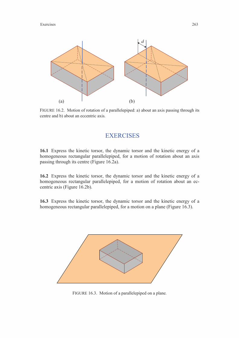
Exercises 263
FIGURE 16.2. Motion of rotation of a parallelepiped: a) about an axis passing through its
centre and b) about an eccentric axis.
EXERCISES
16.1 Express the kinetic torsor, the dynamic torsor and the kinetic energy of a
homogeneous rectangular parallelepiped, for a motion of rotation about an axis
passing through its centre (Figure 16.2a).
16.2 Express the kinetic torsor, the dynamic torsor and the kinetic energy of a
homogeneous rectangular parallelepiped, for a motion of rotation about an ec-
centric axis (Figure 16.2b).
16.3 Express the kinetic torsor, the dynamic torsor and the kinetic energy of a
homogeneous rectangular parallelepiped, for a motion on a plane (Figure 16.3).
FIGURE 16.3. Motion of a parallelepiped on a plane.
d
(a) (b)
264 Chapter 16 Kinetic and Dynamic Torsors. Kinetic Energy
COMMENTS
Kinetics combines the effects of motions with the repartition of masses
over a body or a set of bodies.
The first torsor which was considered is the kinetic torsor which asso-
ciates the effects of masses and velocities. This torsor allows us to express
easily the kinetic energy of a solid.
The second torsor which was studied is the dynamic torsor which com-
bines the effects of masses and accelerations. This torsor is used in the
statement of the fundamental principle of the dynamics (Chapter 19).
The notations which are used for the kinetic torsor( ) T
S and the
dynamic torsor ( ) ,T
S associated to the motion of the solid (S) relatively
to the reference (T) are similar to the notation introduced for denoting the
kinematic torsor ( ) .T
S
The concepts introduced in the present chapter are very important. The
reader will pay a great attention to the way in which these two torsors are
built. To apply the concepts introduced by these torsors, the reader will
have to know the expressions which express the resultant (16.5) and the
moment (16.6) and (16.7), of the kinetic torsor, as well as the expressions
which give the resultant (16.15) and the moment (16.16) and (16.17), of the
dynamic torsor.
These concepts are applied (Exercises) to the case of three motions of
the same rectangular parallelepiped, allowing us to highlight simply the
importance of the conditions of motions.

CHAPTER 17
Change of Reference System
We consider in this chapter the case of a solid (S), whose we study the motions (Figure 17.1) with respect to a reference system ( )1 1 1(1) Ox y z= and with respect to a reference system ( )2 2 2(2) .Ox y z= The two systems of reference (1) and (2) are in motion the one with respect to the other. M is an arbitrary point of the solid (S).
17.1 KINEMATICS OF CHANGE OF REFERENCE
17.1.1 Relation between the Kinematic Torsors
The motion of the solid (S) relatively to the reference (1) is characterized by its
kinematic torsor ( ) 1S , of elements of reduction at point M of the solid (S):
FIGURE 17.1. Change of reference system.
y1
z1
x1
O1
(1)
(S)
M
y2
z2
x2
O2
(2)

266 Chapter 17 Change of Reference System
( ) ( )
( ) ( )
( ) ( ) ( )( )
1 1
1 1
, rotation vector relative to the motion ofthe solid with respect to reference 1 ;
( , ) , velocity vector with respect to 1of the point of the solid .
S S
M S
RS
M tM S
ω =
=
(17.1)
The motion of the solid (S) relatively to the reference (2) is characterized in the
same way by its kinematic torsor ( ) 2S of elements of reduction at the point M:
( ) ( )
( ) ( )
( ) ( ) ( )( )
2 2
2 2
, rotation vector relative to the motion ofthe solid with respect to reference 2 ;
( , ) , velocity vector with respect to 2of the point of the solid .
S S
M S
RS
M tM S
ω =
=
(17.2)
The relative motions of references (1) and (2) are characterized, for example,
by the kinematic torsor ( ) 12 associated to the motion of reference (2) relatively
to reference (1). Its elements of reduction at the point O2 of the reference (2) are:
( ) ( )
( ) ( )
( ) ( ) ( )( )
2
1 12 2
1 12 2
2
, rotation vector relative to the motion ofreference 2 with respect to reference 1 ;
( , ) , velocity vector with respect to 1of the point of reference 2 .
O
R
O tO
ω =
=
(17.3)
From the law of composition of motions (9.39), we have:
( ) ( ) ( ) 1 2 12S S= + . (17.4)
motion of solid (S) motion of solid (S) motion of reference (2)
with respect to reference (1) with respect to reference (2) with respect to reference (1)
The composition of the rotation vectors are deduced from the preceding law of
composition. Hence:
( ) ( ) ( )1 2 12S Sω ω ω= +
. (17.5)
17.1.2 Relation between the Velocity Vectors. Velocity of Entrainment
The relation between the moment-vectors deduced from (17.4) must be
expressed at the same point. Consider the point M of the solid (S). The relation is
thus written: ( ) ( ) ( ) 1 2 1
2MM M PS S= +
. (17.6)
In the formulation of this relation, the moment of the torsor relatively to the motion
of reference (2) with respect to reference (1) is expressed at a point which has:
— to coincide with the point M of the solid (S),
— to belong to reference (2).

17.1 Kinematics of Change of Reference 267
FIGURE 17.2 Coinciding point.
We have denoted it by .MP This point belongs to reference (2) and coincides at
time t with the point M of the solid (S). It is called coinciding point. The point
MP belonging to reference (2) and which coincides at time t with the point M is
not however identical to the point M (Figure 17.2).
Relation (17.6) is written:
( ) ( ) ( )
1 2 12( , ) ( , ) MPM t M t= +
. (17.7)
We notice that ( ) 12MP
is identified with the velocity vector ( )1 ( , )M t with
respect to reference (1), when the point P is motionless relatively to reference (2).
This vector is called the velocity of entrainment of the point M relatively to the
motion of reference (2) with respect to reference (1). This velocity is denoted by ( )12 ( , )e M t . Hence:
( ) ( )1 12 2 ( , )MP e M t=
. (17.8)
Relation (17.7) is put thus in the form:
( ) ( ) ( )
1 2 12( , ) ( , ) ( , )eM t M t M t= +
. (17.9)
The velocity vector of entrainment can be expressed as a function of the velo-
city vector with respect to reference (1) of any point P2 attached to reference (2):
( ) ( ) ( ) ( ) 2
1 1 1 12 2 2 2 2( , ) MP P Me M t R P P= = + ×
.
Thus: ( ) ( ) ( )
1 1 12 2 2 2( , ) ( , ) Me M t P t P Pω= + ×
. (17.10)
O1
M
reference (1)
trajectory of point M
in reference (2 )
points of
reference (2)
O2
x1
z1
z2
y1
y2
x2
(S)
PM
PMPM
268 Chapter 17 Change of Reference System
In the case where the point P2 coincides with the origin O2 of reference (2), the
preceding relation is written:
( ) ( ) ( )
1 1 12 2 2 2( , ) ( , ) ,Me M t O t O Pω= + ×
(17.11)
or ( ) ( ) ( )
1 1 12 2 2 2( , ) ( , )e M t O t O Mω= + ×
. (17.12)
Relation (17.7) between the velocity vectors relatively to the two references
may be finally written in the form:
( ) ( ) ( ) ( )
1 2 1 12 2 2( , ) ( , ) ( , )M t M t O t O Mω= + + ×
. (17.13)
From the definition of the velocity vectors, we can write:
( )( ) ( ) ( )
1 1 11
21 1 2d d d
( , )d d d
M t O M O O O Mt t t
= = +
,
or
( ) ( )( )
11 1
2 2d
( , ) ( , )d
M t O t O Mt
= +
. (17.14)
The comparison of Relations (17.13) and (17.14) shows thus the following
property: ( )
( ) ( )1
2 12 2 2
d( , )
dO M M t O M
tω= + ×
. (17.15)
17.1.3 Composition of Acceleration Vectors
17.1.3.1 Relation
The acceleration vector relatively to reference (1) of the point M is:
( )( )
( )
( )( ) ( ) ( )
11 1
12 1 1
2 2 2
d( , ) ( , )
d
d( , ) ( , ) .
d
a M t M tt
M t O t O Mt
ω
=
= + + ×
(17.16)
— ( )
( )1
2d( , )
dM t
t
is obtained by analogy with Relation (17.15):
( )( ) ( ) ( ) ( )
12 2 1 2
2d
( , ) ( , ) ( , )d
M t a M t M tt
ω= + ×
,
— ( )
( ) ( )
11 1
2 2d
( , ) ( , )d
O t a O tt
= is the acceleration vector relatively to reference
(1) of the point O2,

17.2 Dynamic Torsors 269
( )( )( )
( )( ) ( )
( )
( ) ( ) ( ) ( ) ( )( )
1 1 11 1 1
2 2 2 2 2 2
1 1 2 1 12 2 2 2 2 2
d d d
d d d
( , ) .
O M O M O Mt t t
O M M t O M
ω ω ω
ω ω ω ω
−− ∧ = × + ×
= × + × + × ×
Hence the relation giving the acceleration vector:
( ) ( ) ( ) ( )
( ) ( ) ( ) ( )( )
1 2 1 22
1 1 1 12 2 2 2 2 2
( , ) ( , ) 2 ( , )
( , ) .
a M t a M t M t
a O t O M O M
ω
ω ω ω
= + ×
+ + × + × ×
(17.17)
17.1.3.2 Acceleration of entrainment
The acceleration of entrainment, denoted by ( )1
2( , )ea M t
is the acceleration of
the point MP of reference (2) coinciding at the time considered with the point M:
( ) ( )
1 12 ( , ) ( , )Mea M t a P t=
. (17.18)
From Expression (9.24), the acceleration of entrainment of the point M is expres-
sed as a function of the acceleration vector of the point O2 by the relation:
( ) ( ) ( ) ( ) ( )( )
1 1 1 1 12 2 2 2 2 2 2( , ) ( , )ea M t a O t O M O Mω ω ω= + × + × ×
. (17.19)
17.1.3.3 Acceleration of Coriolis
The acceleration of Coriolis is the term ( ) ( )
1 222 ( , )M tω ×
introduced in Rela-
tion (17.17). Thus: ( ) ( ) ( )
1 1 22 2( , ) 2 ( , )ca M t M tω= ×
. (17.20)
The acceleration of Coriolis is null when the velocity vector of the point M is null
relatively to reference (2).
17.1.3.4 Composition of Accelerations
Relation (17.17) expressing the acceleration vector of the point M may thus be
written in the form:
( ) ( ) ( ) ( )
1 2 1 12 2( , ) ( , ) ( , ) ( , )e ca M t a M t a M t a M t= + +
. (17.21)
This relation constitutes the relation of composition of the acceleration vectors of
a point M in motion relatively to the references (1) and (2).
17.2 DYNAMIC TORSORS
In this section, we study how the dynamic torsor of a solid (S) is transformed
when we change a reference (1) for a reference (2). This change of reference
270 Chapter 17 Change of Reference System
introduces two new torsors: the inertia torsor of entrainment and the inertia
torsor of Coriolis.
17.2.1 Inertia Torsor of Entrainment
The inertia torsor of entrainment of the solid (S) relatively to the motion of the
reference (2) with respect to the reference (1), denoted by ( )( ) 1
2 ,S is the torsor
defined over this solid and associated to the field of sliders whose the vector
density (relative to the mass) at every point of the solid is equal to the acce-
leration vector of entrainment of this point relatively to the motion of the
reference (2) with respect to the reference (1).
The inertia torsor of entrainment ( )( ) 1
2 ,S is thus associated to the field of
sliders of resultants:
( )M S∀ ∈ ( )
12d ( ) ( , )d ( )eR M a M t m M=
, (17.22)
where the acceleration vector of entrainment is expressed by Relation (17.19).
The elements of reduction of the inertia torsor of entrainment are thus:
1. Resultant
( )( ) ( )
( )
1 12 2 ( , ) d ( )
SeR S a M t m M=
. (17.23)
Hence:
( )( ) ( ) ( ) ( ) ( )( )1 1 1 1 12 2 2 2 2 2 2( , )R S m a O t O G O Gω ω ω = + × + × ×
,
or
( )( ) ( )1 12 2 ( , )eR S ma G t=
. (17.24)
2. Moment-vector
Expression (17.19) of the acceleration vector of entrainment of a point M of
the solid leads to express the moment-vector at a point attached to the reference
(2), the point O2 for example:
( )( ) ( )
( )2
1 12 2 2 ( , ) d ( )O
SeS O M a M t m M= ×
. (17.25)
Thus:
( )( ) ( ) ( ) ( ) ( ) ( ) ( ) 2 2 2
1 1 1 1 12 2 2 2 2 2( , )O O OS m O G a O t S Sω ω ω= × + + ×
, (17.26)
where the operator of inertia ( )2O S has its representative matrix defined from
the matrix of inertia at the mass centre by applying the relations of Huyghens
(Relations (15.25)).

17.2 Dynamic Torsors 271
17.2.2 Inertia Torsor of Coriolis
The inertia torsor of Coriolis of the solid (S) relatively to the motion of the
reference (2) with respect to the reference (1), denoted by ( )( ) 1
2 S , is the torsor
defined over this solid and associated to the field of sliders whose the vector
density (relative to the mass) at every point of the solid is equal to the acce-
leration vector of Coriolis of this point relatively to the motion of the reference
(2) with respect to the reference (1).
This torsor is thus associated to the field of sliders of resultant:
( )M S∀ ∈ ( )
12d ( ) ( , )d ( )cR M a M t m M=
, (17.27)
where the acceleration vector of Coriolis is expressed by (17.20). In this relation,
the velocity vector ( )2 ( , )M t can be expressed as a function of the velocity
vector of a particular point of the solid (S), for example the mass centre. The ace-
leration vector of Coriolis has then for expression:
( ) ( ) ( ) ( )
1 1 2 22 2( , ) 2 ( , )c Sa M t G t GMω ω = × + ×
. (17.28)
The elements of reduction of the inertia torsor of Coriolis are:
1. Resultant
( )( ) ( )
( )
1 12 2 ( , ) d ( )
ScR S a M t m M=
. (17.29)
Hence from (17.28): ( )( ) ( ) ( )
1 1 22 22 ( , )R S m G tω= ×
, (17.30)
or ( )( ) ( )1 1
2 2 ( , )cR S ma G t= . (17.31)
2. Moment-vector
Expression (17.28) of the acceleration vector of Coriolis of a point M of the
solid leads to express the moment vector at the mass centre of the solid:
( )( ) ( )
( )
1 12 2 ( , ) d ( )G
ScS GM a M t m M= ×
. (17.32)
Thus:
( )( ) ( ) ( )( )( )
1 1 22 22 d ( )G S
S
S GM GM m Mω ω = × × × . (17.33)
Considering the property of the double vector product, we have: ( ) ( )( ) ( )( ) ( )1 2 1 22 2S SGM GM GM GMω ω ω ω × × × = × ⋅
,
and ( )( ) ( ) ( ) ( )( )1 1 12 2 2GM GM GM GM GM GMω ω ω× × = −⋅ ⋅
.
272 Chapter 17 Change of Reference System
Finally:
( ) ( )( )( ) ( )( ) ( )( ) ( )
1 22
2 1 2 1 22 2 .
S
S S
GM GM
GM GM GM
ω ω
ω ω ω ω
× × ×
= × − × × ×
The moment at the mass centre (17.33) is thus written as:
( )( ) ( )
( ) ( ) ( ) ( ) ( )21 1 2 2 12 2 22 d ( ) 2G S S G
S
S GM m M Sω ω ω ω = × + × .
In this expression, the integral is the moment of inertia of the solid (S) with
respect to the mass centre: IG(S). The moment of the inertia torsor of Coriolis is
thus written:
( )( ) ( ) ( ) ( ) ( ) ( )1 1 2 2 12 2 22 ( ) 2G G S S GS I S Sω ω ω ω= × + ×
. (17.34)
Note. The inertia torsors of entrainment and of Coriolis can be generalized to the
case of a system of solids by doing the sum of torsors defined on every solid.
17.2.3 Relation between the Dynamic Torsors Defined Relatively to Two Different References
Express the dynamic torsors relative to the motions of the solid (S) with
respect to two references (1) and (2). We have from (16.14):
— motion of (S) relatively to (1), dynamic torsor ( ) 1
S with:
( ) ( )1 1( , )SR ma G t= , (17.35)
— motion of (S) relatively to (2), dynamic torsor ( ) 2
S with:
( ) ( )2 2 ( , )SR ma G t= . (17.36)
It results from the law of composition of the accelerations (Relation (17.21)) and
from Expressions (17.24) and (17.31) that:
( ) ( ) ( )( ) ( )( ) 1 2 1 12 2S SR R R S R S= + +
. (17.37)
A similar relation exists with the moment vectors. Hence the expression of
reference change for the dynamic torsors:
( ) ( ) ( )( ) ( )( ) 1 2 1 12 2S S S S= + + . (17.38)
This expression gives the relation which exists between the dynamic torsors rela-
tively to the motions of a same solid (S) with respect to the reference (1) and with
respect to the reference (2).
Comments 273
COMMENTS
This chapter is interested in the motions of a solid (S) with respect to
two reference systems (1) and (2). Within this context, the concept of coin-
ciding point and the concept of velocity of entrainment are important
concepts. The expression of the velocity vector of entrainment is obtained
simply by using the concept of kinematic torsor associated to the motion of
one of the references with respect to the other. The relation between the
dynamic torsors associated to the motions of the solid (S) with respect to
the reference (1) and to the reference (2) leads to introduce the inertia
torsors of entrainment and of Coriolis. The concepts of these torsors can
appear somewhat complex to handle. In fact, these concepts are necessary
to formalize the fundamental law of dynamics expressed in different
reference systems (Chapter 19). In practice, these concepts will be
introduced implicitly, without using the relations established in the present
chapter, when the dynamic torsors will be expressed directly with respect to
the different reference systems.
Thus, in a first approach, the reader will simply endeavour the deve-
lopment of the various concepts which are introduced. These notions will
be then studied thoroughly and progressively with the development of the
knowledge of the reader.


Part V
Dynamics of Rigid Bodies
The motions of bodies having been characterized, the mechanical
actions having been analyzed, it now remains to understand how the
mechanical actions act to produce such or such motion. This problem
is solved starting from the fundamental principle of dynamics. This
principle will be applied to the analysis of various elementary motions.
The application of the fundamental principle gives access to the
nature of the motions as well as to the characteristic parameters of the
actions induced by the connections. The application of the equations
of Lagrange will allow us to acquire a systematic tool to derive the
equations of motions.

CHAPTER 18
The Fundamental Principle of Dynamics and its Consequences
18.1 FUNDAMENTAL PRINCIPLE
18.1.1 Statement of the Fundamental Principle of Dynamics
There exists at least a reference system, called Galilean reference, which will be
denoted by (g), such as, at any moment and for any material set (D), the dynamic
torsor associated to the motion of the set (D) relatively to this reference system is
equal to the torsor of mechanical actions which are exerted on the set (D).
This principle is written in the form:
( ) ( )g
D D= , (18.1)
where ( )D is the torsor which represents the whole of the mechanical actions
exerted on the set (D).
The fundamental principle of dynamics, justified by the agreement between the
theoretical results derived from this principle and the experimental results obser-
ved, states the existence of at least a Galilean reference system. We clarify, in the
following subsection, the relations which exist between the Galilean references.
18.1.2 Class of Galilean Reference Systems
Let (1) and (2) be two Galilean references (Figure 18.1). We derived in the
case of the motions of a solid (S) relatively to two references (Relation (17.38)):
( ) ( ) ( )( ) ( )( ) 1 2 1 12 2S S S S= + + .
So that the fundamental relation (18.1) has the same form relatively to the two

278 Chapter 18 The Fundamental Principle and its Consequences
FIGURE 18.1. Galilean reference systems.
references, the torsor of the mechanical actions being unchanged while passing
from the reference (1) to the reference (2), it is necessary and sufficient that:
( )( ) 12 0S = , (18.2)
( )( ) 12 0S = . (18.3)
Expressions (17.30) and (17.34) of the elements of reduction of the torsor of
Coriolis at the mass centre shows that the second relation (18.3) is satisfied if and
only if ( )12 0ω =
. Hence the first result: two Galilean references are animated the
one with respect to the other by a motion of translation.
Expressions (17.24) and (17.26) of the elements of reduction of the torsor of
entrainment at the point O2 shows then that the first relation (18.2) is satisfied if:
( )12( , ) 0a O t =
. (18.4)
The velocity vector at the point O2 is thus a constant vector: the motion of the
reference (2) is a motion of uniform rectilinear translation with respect to the
reference (1).
This result shows that the fundamental principle of dynamics admits the
existence of a class of Galilean references:
There exists an infinity of Galilean references. Two Galilean references move
the one with respect to the other with a motion of uniform rectilinear translation.
The fundamental principle has an invariant expression (18.1) relatively to any of
these Galilean references.
18.1.3 Vector Equations Deduced from the Fundamental Principle
The fundamental relation of dynamics (18.1) leads to the two vector equations:
y1
z1
x1
O1
(1) x2
y2
z2
O2
(2)
(S)

18.1 Fundamental Principle 279
( ) ( )g
DR R D=
, (18.5)
( ) ( )g
P PD D=
, (18.6)
where P is an arbitrary reference point.
1. Equation of the resultantThe resultant of the dynamic torsor expressed in (16.19) leads to rewrite Equa-
tion (18.5) of the resultant in the form:
( ) ( , ) ( )g
ma G t R D= . (18.7)
This result is usually stated in the form:
The general resultant of the mechanical actions exerting on a material set is
equal to the product of the mass of this set by the acceleration vector of the mass
centre of this set relatively to a Galilean reference system.
2. Equation of the momentIn the case of the motion of a solid (S), the equation of the moment is written,
from (16.16):
( ) ( ) ( ) ( ) ( ) ( ) ( , ) ( )g g gg
PP PS S Sm PG a P t S S Sω ω ω× + + × = . (18.8)
This expression is simplified, when the equation of the moment is expressed at the
mass centre:
( ) ( ) ( ) ( ) ( ) ( )g g g
GG GS S SS S Sω ω ω+ × = . (18.9)
In the case of a set of bodies, the moment of the dynamic torsor is expressed
according to Relation (16.20).
Moreover, the equation of the moment may be expressed while taking account
of Relation (16.23) as a function of the kinetic torsor in the form:
( )
( ) d( )
d
gg
G G SSt
=
. (18.10)
18.1.4 Scalar Equations Deduced from the Fundamental Principle
The vector equations of the resultant and of the moment lead each one to 3
scalar equations, that is a total of 6 scalar equations for a given material set. The
choice of the bases (which can be different) to express the equation of the
resultant and that one of the moment, and the choice of the point at which the
equation of the moment will be expressed, will be carried out so as to simplify
calculation as well as possible. In the case of elementary motions, these choices
are generally obvious. In the case of complex motions, these choices are not
always simple to take. They will be generally implemented considering different
successive tests.
280 Chapter 18 The Fundamental Principle and its Consequences
18.2 MUTUAL ACTIONS
18.2.1 Theorem of Mutual Actions
The theorem of mutual actions stated within the framework of statics (Section
14.2.3) can be transposed to the context of the dynamics of bodies. We establish
hereafter this relation considering the notations of Section 14.2.3.
Applying the fundamental law to the two material sets (D1) and (D2), we have:
( ) 1
1 1 2 11 2 1g
DD D D DD D D= → = + →∪ → , (18.11)
( ) 2
2 2 1 21 2 2g
DD D D DD D D= → = + →∪ → . (18.12)
Applying the fundamental law of dynamics to the union ( )1 2 ,D D∪ we have:
( ) 1 2 1 2 1 2
g
D D D D D D∪ = ∪ → ∪ , (18.13)
or taking account of properties (11.4) and (16.17):
( ) ( ) 1 2 1 2 1 1 2 2g g
D D D D D D D D+ = +∪ → ∪ → . (18.14)
Comparing the three relations (18.11), (18.12) and (18.14), we obtain well the
relation which translates the theorem of mutual actions:
2 1 1 2D D D D→ = − → . (18.15)
This relation associated to Expression (11.9) of the mechanical actions exerted
on a given material set leads to a global relation of the actions of gravitation,
actions of contact and electromagnetic action exerted on a given set:
2 12 1 2 1
1 21 2 1 2 .
D DD D D D
D DD D D D
→+ + =→ →
→− + +→ →
(18.16)
Relation (18.15) in fact is extended to each type of mechanical actions consi-
dered separately. Thus:
2 1 1 2D D D Dϕ ϕ→ →= − , (18.17)
whatever the physical law ϕ exerted on the two sets ( ,ϕ = or ) .
Thus, the properties of the mutual actions established in the case of statics
(Section 14.2.3) can be transposed to the case of the dynamics of sets of solids.
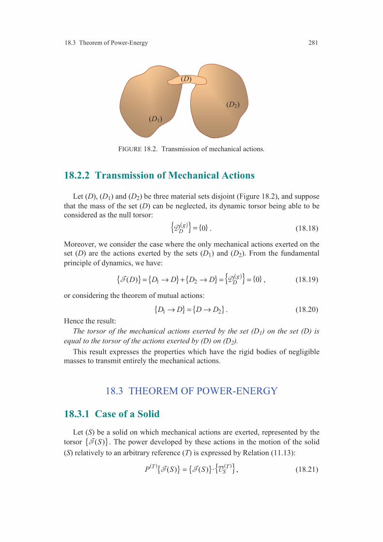
18.3 Theorem of Power-Energy 281
FIGURE 18.2. Transmission of mechanical actions.
18.2.2 Transmission of Mechanical Actions
Let (D), (D1) and (D2) be three material sets disjoint (Figure 18.2), and suppose
that the mass of the set (D) can be neglected, its dynamic torsor being able to be
considered as the null torsor:
( ) 0g
D= . (18.18)
Moreover, we consider the case where the only mechanical actions exerted on the
set (D) are the actions exerted by the sets (D1) and (D2). From the fundamental
principle of dynamics, we have:
( ) 1 2( ) 0g
DD D D D D= → + → = = , (18.19)
or considering the theorem of mutual actions:
1 2D D D D→ = → . (18.20)
Hence the result:
The torsor of the mechanical actions exerted by the set (D1) on the set (D) is
equal to the torsor of the actions exerted by (D) on (D2).
This result expresses the properties which have the rigid bodies of negligible
masses to transmit entirely the mechanical actions.
18.3 THEOREM OF POWER-ENERGY
18.3.1 Case of a Solid
Let (S) be a solid on which mechanical actions are exerted, represented by the
torsor ( )S . The power developed by these actions in the motion of the solid
(S) relatively to an arbitrary reference (T) is expressed by Relation (11.13):
( ) ( ) ( ) ( )T TSP S S= ⋅ , (18.21)
(D2)
(D1)
(D)

282 Chapter 18 The Fundamental Principle and its Consequences
where ( ) TS is the kinematic torsor relatively to the motion of the solid (S) with
respect to the reference (T).
In the case where the reference (T) is a Galilean reference (g), the fundamental
law of dynamics allows us to write:
( ) ( ) ( ) ( )g gg
S SP S = ⋅ . (18.22)
Taking account of Expression (16.32), we obtain:
( ) ( )c
d( ) ( )
d
g gP S E S
t= . (18.23)
Hence the theorem of power-energy:
In any motion of a solid with respect to a Galilean reference, the power deve-
loped by the mechanical actions exerted on this solid is, at any moment, equal to
the derivative with respect to time of the kinetic energy of the solid relatively to
the Galilean reference.
This theorem can take another form while introducing into Expression (18.23)
the work of the mechanical actions exerted on the solid (S) between the instants t1and t2. From the relation of definition (11.24) of work, Expression (18.23) is
written:
( ) ( ) ( )1 2 c 2 c 1( , ) ( ) ( )
g g gW t t E t E t= − . (18.24)
Hence the new statement, known under the name of theorem of kinetic energy:
In any motion of a solid with respect to a Galilean reference, the work, between
two instants, of the mechanical actions acting on the solid is equal to the
variation, during the motion, of the kinetic energy of the solid between these two
instants.
Note. The theorem of power-energy, deduced from the fundamental principle of
dynamics, does not bring any new information. Relation (18.23) leads to an equa-
tion which is a linear combination of the six scalar equations deduced from the
fundamental law (18.1), combination which is sometimes more interesting to use.
18.3.2 Case of a Set of Bodies
Let (D) be a set of n solids (Subection 11.3.6 and Figure 11.4). The actions
exerted on the solid (Si) are (Relation (11.38)):
1
( )
n
i i i i j i
ji
S S S D S S S
=≠
= → = → + → , (18.25)
and the theorem of power-energy (18.22) is written for each solid:
( ) ( )c
d( ) ( )
d
g gi iP S E S
t= . (18.26)

18.3 Theorem of Power-Energy 283
By summation on the set of the solids (Si), we obtain, taking account of Relation
(16.30):
( ) ( ) c
1
d( ) ( )
d
ng g
i
i
E D P St
=
=
. (18.27)
Thus:
( ) ( ) ( ) c
1 1 1
d ( )d
n n ng g g
i j i
i i ji
E D P D S P S St
= = =≠
= → + → , (18.28)
external actions internal actions
with:
( ) ( )c c
1
( ) ( )
ng g
i
i
E D E S
=
= . (18.29)
Hence the theorem of power-energy for a set of solids:
The derivative with respect to time of the kinetic energy of a set of solids,
relatively to a Galilean reference, is equal to the sum of the powers developed in
this reference by the mechanical actions exerted on each solid by the other solids
and by the material systems external to the set of the solids.
The integration between times t1 and t2 of Relation (18.28) leads to the follo-
wing formulation of the theorem of kinetic energy for a set of solids:
( ) ( ) ( ) ( ) 1 2 1 2
c 2 c 1 , ,
1 1 1
( , ) ( , )
n n ng gg g
i j it t t t
i i ji
E D t E D t W D S W S S
= = =≠
− = → + → . (18.30)
Note. It is important to observe that the theorem of power-energy or that of
kinetic energy considers the external and internal mechanical actions. In contrast,
we shall see (Section 20.2) that the fundamental principle applied to a set of solids
introduces only the external mechanical actions.
18.3.3 Mechanical Actions with Potential Energy
We consider the case where the mechanical actions exerted on a material set
admit a potential energy in the Galilean reference (g). We have then (Relation
(11.19)):
( ) ( )p
d( ) ( , )
d
g gP D E D t
t= − . (18.31)
By substitution into Expression (18.27) of the theorem of power-energy, we obtain:
( ) ( )
c pd d
( , ) ( , ) 0d d
g gE D t E D t
t t+ = . (18.32)
Thus by integration:
284 Chapter 18 The Fundamental Principle and its Consequences
( ) ( ) ( ) c p m( , ) ( , ) ( )
g g gE D t E D t E D+ = , (18.33)
where ( )m ( )g
E D is a function independent of time, called mechanical energy of the
set (D) relatively to the Galilean reference (g). Hence the theorem of conser-
vation of energy:
In the case where the mechanical actions exerted on a material set admit
relatively to a Galilean reference a potential energy, the sum of the kinetic energy
and of this potential energy is in a Galilean reference a function independent of
time, called mechanical energy of the material set in the reference under con-
sideration.
18.4 APPLICATION OF THE FUNDAMENTAL
PRINCIPLE TO THE STUDY OF THE MOTION OF A
FREE BODY IN A GALILEAN REFERENCE
The analysis which will be implemented in this section can be applied in
particular to the motions of projectiles, planets, satellites, etc.
18.4.1 General Problem
Consider a solid (S) of mass m and mass centre G, free (Figure 18.3) relatively
to a Galilean reference (g), at which the coordinate system ( )/ , , g g g gO i j k
is
attached. The motion of solid (S) with respect to the reference (g) is defined by:
— the position of a point of the solid: we choose the mass centre G of the solid
of which the position will be characterized relatively to the coordinate system
attached to (g) by three coordinates (Cartesian, cylindrical, spherical or other
ones) which we will denote in a general way by p1, p2, p3 (the position vector
gO G
of the mass centre is a function of the coordinates p1, p2, p3);
— the orientation of the solid with respect to the reference (g): we choose a
trihedron ( )S S SGx y z attached to the solid (S), such that this trihedron is a prin-
cipal trihedron of inertia at the point G. The orientation of this trihedron is
characterized for example by the Eulerian angles ψ, θ, ϕ.
Let ( )S be the torsor which represents the whole of the mechanical actions
exerted on the solid. To study the motion of (S) with respect to the Galilean refe-
rence (g), we have the fundamental law of dynamics:
( ) ( )g
S S= , (18.34)
which leads to the vector equations of the resultant and of the moment.
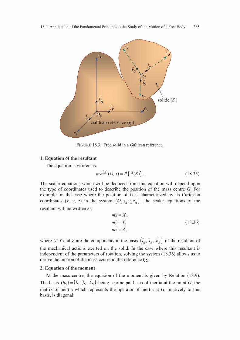
18.4 Application of the Fundamental Principle to the Study of the Motion of a Free Body 285
FIGURE 18.3. Free solid in a Galilean reference.
1. Equation of the resultant
The equation is written as:
( ) ( , ) ( )g
ma G t R S= . (18.35)
The scalar equations which will be deduced from this equation will depend upon
the type of coordinates used to describe the position of the mass centre G. For
example, in the case where the position of G is characterized by its Cartesian
coordinates (x, y, z) in the system ( ) ,g g g gO x y z the scalar equations of the
resultant will be written as:
,
,
,
mx X
my Y
mz Z
=
=
=
(18.36)
where X, Y and Z are the components in the basis ( ), , g g gi j k
of the resultant of
the mechanical actions exerted on the solid. In the case where this resultant is
independent of the parameters of rotation, solving the system (18.36) allows us to
derive the motion of the mass centre in the reference (g).
2. Equation of the moment
At the mass centre, the equation of the moment is given by Relation (18.9).
The basis ( )( ) , , S S S Sb i j k=
being a principal basis of inertia at the point G, the
matrix of inertia which represents the operator of inertia at G, relatively to this
basis, is diagonal:
Oggi
gj
gk
yg
zg
xg
Galilean reference (g )
zS
yS
G
xS
Sj
Si
Sk
solide (S )
286 Chapter 18 The Fundamental Principle and its Consequences
( )0 0
( ) 0 0
0 0
SbG
A
S B
C
=
I . (18.37)
The instantaneous vector of rotation and its derivative with respect to time relative
to the motion of the solid (S) with respect to the reference (g) are expressed, in the
basis (bS), according to Expressions (9.78) and (9.81). Hence:
( ) ( ) 1 2 3
gG S S SSS A i B j C kω ω ω ω= + +
, (18.38)
( ) ( ) ( ) ( ) ( ) ( ) 2 3 1 3 1 2
g gG S S SS SS C B i A C j B A kω ω ω ω ω ω ω ω× = − + − + −
. (18.39)
Expression (18.9) of the moment at the point G leads thus to the scalar equations:
( )
( )
( )
1 2 3
2 1 3
3 1 2
,
,
,
A C B L
B A C M
C B A N
ω ω ω
ω ω ω
ω ω ω
+ − =
+ − =
+ − =
(18.40)
where L, M and N are the components, in the basis (bS), of the moment at G of the
mechanical actions exerted on the solid. In the general case, these components are
functions of the variables , , , , , , ,i ip p ψ θ ϕ ψ θ ϕ . Analytical solutions will be
obtained only for some simple particular cases. If the components L, M and N are
independent of the parameters , i ip p , Equations (18.40) will be decoupled from
Equations (18.35) of the resultant. Solving Equations (18.40) will then allow us to
determine the motion of rotation of the solid.
18.4.2 Particular Cases
18.4.2.1 Case where the Resultant of the Mechanical Actions
is a Constant Vector
We study here the case where the resultant of the mechanical actions exerted
on the solid is a constant vector in the reference (g):
( )R S R=
. (18.41)
Equation (18.35) of the resultant shows that the acceleration vector of the mass
centre is constant:
( )0( , )g R
a G t am
= =
. (18.42)
The motion was studied in Section 7.3 of Chapter “Kinematics of Point”. The
trajectory of the mass centre is either a straight line or a parabola.
An example of this type of motion is given by a solid submitted to the field
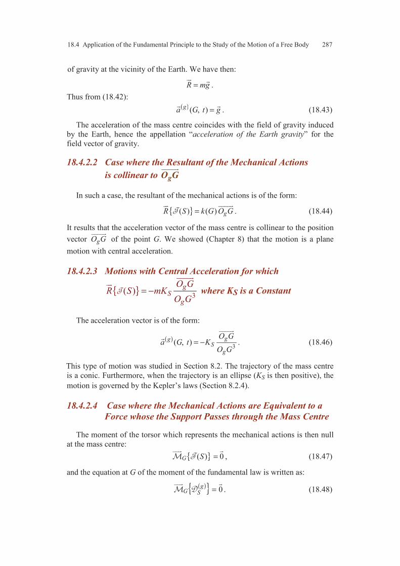
18.4 Application of the Fundamental Principle to the Study of the Motion of a Free Body 287
of gravity at the vicinity of the Earth. We have then:
R mg=
.
Thus from (18.42):
( ) ( , )g
a G t g=
. (18.43)
The acceleration of the mass centre coincides with the field of gravity induced
by the Earth, hence the appellation “acceleration of the Earth gravity” for the
field vector of gravity.
18.4.2.2 Case where the Resultant of the Mechanical Actions
is collinear to
gO G
In such a case, the resultant of the mechanical actions is of the form:
( ) ( ) gR S k G O G=
. (18.44)
It results that the acceleration vector of the mass centre is collinear to the position
vector gO G
of the point G. We showed (Chapter 8) that the motion is a plane
motion with central acceleration.
18.4.2.3 Motions with Central Acceleration for which
3
( )g
S
g
O GR S mK
O G= −
where KS is a Constant
The acceleration vector is of the form:
( )3
( , )gg
S
g
O Ga G t K
O G= −
. (18.46)
This type of motion was studied in Section 8.2. The trajectory of the mass centre
is a conic. Furthermore, when the trajectory is an ellipse (KS is then positive), the
motion is governed by the Kepler’s laws (Section 8.2.4).
18.4.2.4 Case where the Mechanical Actions are Equivalent to a
Force whose the Support Passes through the Mass Centre
The moment of the torsor which represents the mechanical actions is then null
at the mass centre:
( ) 0G S =
, (18.47)
and the equation at G of the moment of the fundamental law is written as:
( ) 0g
G S =
. (18.48)

288 Chapter 18 The Fundamental Principle and its Consequences
Thus, from (16.23):
( )
( ) d0
d
gg
G St=
. (18.49)
That leads to:
( ) ( )0
g gG S σ=
, (18.50)
where ( )0gσ
is a vector independent of time in the reference (g). This expression is
also written from (16.7) as:
( ) ( ) ( )0
g gG SS ω σ=
. (18.51)
In the particular case where the solid has a spherical symmetry of centre G, the
principal moments of inertia are equal ( A B C= = ), and we have:
( ) ( ) ( )g gG S SS Aω ω=
, hence
( )( )0g
gS A
σω =
. (18.52)
The instantaneous vector of rotation ( )gSω
is thus a vector independent of time in
the reference (g). In the case where the vector ( )0gσ
is the null vector, the vector of
rotation is also null. Thus, we deduce the following results.
The motion, with respect to a Galilean reference, of a solid having a spherical
symmetry and submitted in this reference to mechanical actions equivalent to a
force whose the support passes through the centre of symmetry is:
— either a motion of translation,
— or a motion of uniform rotation about a mobile axis, which passes through
the centre of symmetry and which keeps a direction fixed in the Galilean reference.
The motion of the centre of symmetry depends on the resultant of the equi-
valent force exerted on the solid.
18.5 APPLICATION TO THE SOLAR SYSTEM
18.5.1 Galilean Reference
The solar system is constituted (Figure 18.4) of the Sun and of multiple planets
including nine principal planets: Mercure, Venus, Mars, Jupiter, Saturn, Uranus,
Neptune, Pluto and the Earth. Several planets are accompanied by smaller
satellites which turn around them: thus the Moon is the natural satellite of the
Earth. These planets have dimensions much lower than that of the Sun. The other
planets have dimensions still much lower and are called asteroids. The Sun
represents 99.87% of the total mass of the Sun system.
The distance between the solar system and the nearest star (Proxima Centauri)
is enormous compared to the dimensions of the Sun system. Indeed the light

18.5 Application to the Solar System 289
FIGURE 18.4. The solar system seen from a point of space.
emitted by the Sun reaches the Earth in 8 minutes and Pluto (planet furthest away
from the Sun) in less than 6 hours, whereas it takes 4 years to reach Proxima
Centauri. From this, it results that the solar system can be considered as isolated in
the Universe and that it is possible to neglect the mechanical actions exerted by
the other solar systems on our solar system.
Thus, it results that the torsor of the mechanical actions exerted on the solar
system can be considered as being null, and the equation of the resultant of the
fundamental principle is written as:
( )Sso Sso( ) 0
gm a G =
(18.53)
where mSso and GSso are respectively the mass and the mass centre of the solar
system.
This equation shows that the mass centre of the solar system is either motion-
less, or animated by a rectilinear and uniform motion with respect to a Galilean
reference. So, it results (Section 18.1.2) that the mass centre of the solar system is
itself a point attached to a Galilean reference (g), point which we can take as
origin of the reference. The axes of the reference are then chosen so has to have
fixed directions of the axes with respect to “fixed” stars: stars very far away from
the solar system and appearing for an observer of the solar system under fairly
constant angular distances. The mass of the Sun representing the near totality of
the mass of the solar system, the mass centre of the solar systems coincides
practically with the mass centre of the Sun, itself coinciding fairly with the centre
of the Sun considered as a sphere.
Thus the existence of a Galilean reference (g) is materialized as having:
— for origin, the centre of Sun;
— directions of axes ( ), , g g gi j k
which are fixed with respect to directions of
fixed stars.
Earth
Sun Mercure
Mars
Jupiter
Venus
Saturn
Uranus
Neptune
Pluto
290 Chapter 18 The Fundamental Principle and its Consequences
Any other reference (Section (18.1.2), in motion of uniform rectilinear trans-
lation with respect to this reference, is also a Galilean reference.
18.5.2 Motion of Planets
At first approximation, the planets and the Sun can be assimilated to bodies
having a spherical symmetry. Thus, in accordance with the laws of the gravitation
(Chapter 12), with the results of Subsection 18.4.2.3 of the present chapter and
with the results established in Section 8.2 of Chapter 8, the centre of the planets
describe ellipses having the centre of the Sun as focus. These ellipses are fairly
circular and approximately located in the same plane. The orbits of the planets are
described in the same direction and the laws of the motions of the planet centres
are governed by the Kepler’s laws (Section 8.2.4).
Moreover, in accordance with the results of Subsection 18.4.2.4, the planets are
animated by a motion of rotation about a mobile axis keeping a direction fixed in
the Galilean reference (g). This motion of rotation is called motion of sidereal
proper rotation.
18.5.3 The Earth in the Solar System
We specify in this section, the motion of the Earth of which the general cha-
racteristics were considered in the preceding subsection.
The law of the gravitation and its consequences (Chapter 12) allow us to
conclude that the mechanical actions exerted on the Earth are reduced to the
action of gravitation exerted by the Sun. Thus:
(Te) So Te= →. (18.54)
This description comes to neglect on the one hand the gravitational attractions of
the stars other than the Sun and of the planets, and on the other hand the actions
other than the gravitation.
If the Sun and the Earth are assimilated to solid spheres homogeneous by con-
centric layers, it is shown (Exercise 12.7) that the action of gravitation exerted by
the Sun on the Earth is a force of which the support passes through the centre of
the Earth and of resultant:
( )
TeSo Te 3
Te So
So TeSoO O
R Km mO O
=→
, (18.55)
where K is the constant of gravitation. All occurs as if the masses of the Sun and
of the Earth were concentrated respectively at their centres.
This model and the results of Subsections 18.4.2.3 and 18.4.2.4 allow us to
justify the motion of the Earth assimilated to a body with spherical symmetry
(motion similar to the motions of the other planets, Sub-section 18.5.2).

Comments 291
1. The centre of the Earth describes an elliptic trajectory of which one of the
foci is the centre of the Sun and of which the plane is called plane of the ecliptic.
The areal velocity of the centre of the Earth along its trajectory and relatively to
the Sun centre is constant. The motion of the Earth along its trajectory is gover-
ned by the Kepler’s laws.
2. The Earth is animated by a motion of sidereal proper rotation about an axis
( )Te Te, O k
which forms a constant angle of 23°27' with the normal to the plane of
the ecliptic. The axis ( )Te Te, O k
is the axis South-North of the poles. The angular
velocity of sidereal proper rotation is defined by:
( )TeTe
gkω Ω Ω= =
, (18.56)
with
4 120,729 10 rad s
86164
πΩ − −= = × ,
owing to the fact that the Earth achieves a rotation on itself in 23h56min04s.
The motion of the Earth is schematized in Figure 18.5. The inclination of the
axis of sidereal rotation with respect to the normal direction of the plane of the
ecliptic leads to sunning daily durations varying according to the latitude and the
period of the year.
The 24 hours duration for one day combines the effect of the proper rotation
with the motion of the Earth on its trajectory.
FIGURE 18.5. Motion of the Earth.
COMMENTS
The fundamental principle of the dynamics is the key for the analysis of
a problem of Mecanics of Rigid Bodies. Its formulation while considering
the concept of torsors leads to the equality of the dynamic torsor with the
torsor which represents the whole of the mechanical actions exerted on the
material set considered, and this when the motion is analyzed with respect
Earth
Sun
23°27'
axis South-North
292 Chapter 18 The Fundamental Principle and its Consequences
to a Galilean reference. The fundamental principle leads thus to two vector
equalities, that is a total of six scalar equations for a given material set.
The fundamental principle was then applied to the analysis of the motion
of free body, with for object to find a Galilean reference system. This
reference has for origin the centre of the solar system, coinciding practi-
cally with the centre of the Sun, and axis directions which are fixed with
respect to fixed stars. The chapter gives then some elements about the
motions of the planets and of the Earth in the solar system.
The reader will pay all his attention on the development implemented
throughout this chapter.
CHAPTER 19
The Fundamental Equation of Dynamics in Different References
19.1 GENERAL ELEMENTS
19.1.1 Fundamental Equation of Dynamics in a Non Galilean Reference
We consider a reference (R) animated with respect to the Galilean reference (g)
by a motion which is known but arbitrary and we seek how the fundamental
principle of dynamics is written in the non Galilean reference (R).
The fundamental principle of dynamics applied to the motion of a solid (S) is
written as:
( ) ( ) ( )g g
S S= , (19.1)
where ( ) ( )g
S is the torsor of the mechanical actions exerted on the solid (S)
and measured in the Galilean reference (g). Thus, it results that the dynamic torsor
associated to the motion of the solid (S) with respect to the reference (R) is written
from Relations (19.1) and (17.38) as:
( ) ( ) ( )( ) ( )( ) ( )g ggR
S R RS S S= − − , (19.2)
or ( ) ( ) ( )R R
S S= , (19.3)
setting: ( ) ( ) ( )( ) ( )( ) ( ) ( )
g ggRR RS S S S= − − . (19.4)
Equation (19.3) thus obtained is similar to the fundamental equation (19.1)
which is expressed in a Galilean reference. Expression (19.4) shows that the

294 Chapter 19 The Fundamental Equation of Dynamics in Different References
torsors ( )( ) gR S− and ( )( ) g
R S− represent physical entities similar to the
entity which the torsor ( ) ( )g
S represents. They are not however mechanical
actions with the proper sense, because they are not exerted by material systems. It
is however usual to say that these torsors represent actions called inertia action of
entrainment for the torsor ( )( ) gR S− and inertia action of Coriolis for the torsor
( )( ) gR S− . These actions must be considered as fictitious actions, which express
the effect of the motion of a non Galilean reference with respect to a Galilean
reference. From the established expressions, these fictitious actions do not depend
on the Galilean reference considered. Expressions (19.3) and (19.4) can then be
stated in the following way.
In a non Galilean reference, the fundamental principle of the dynamics can be
written (19.3) in a similar way as in a Galilean reference, on condition to intro-
duce the torsor sum of the mechanical actions exerted on the solid (S), expressed
in a Galilean reference, and of two torsors representing fictitious actions: the
inertia action of entrainment and the inertia action of Coriolis, fictitious actions
which take account of the motion of the non Galilean reference with respect to a
Galilean reference.
19.1.2 The Reference Systems used in Mechanics
1. In the preceding chapter, we highlighted the existence of a Galilean reference
(g) having the Sun centre for origin and axis directions which are fixed with
respect to directions of fixed stars. Moreover, the plane of the ecliptic is fixed in
this reference. It is thus possible (Figure 19.1) to choose as Galilean trihedron, the
trihedron of origin OSo the Sun centre and of plane ( )So , , g gO i j
coinciding with
the plane of ecliptic.
2. A second reference used is the reference associated to the motion of trans-
lation of the Earth on its trajectory. This reference which we shall denote by (Te)
is called geocentric reference.
At this reference system, we associate the trihedron (Figure 19.1) of which:
— the origin is the centre OTe of the Earth,
— the axis ( )Te Te, O k
is the axis of sidereal proper rotation of the Earth and
the axis ( )Te Te, O i
is contained in the plane of the ecliptic.
So, the trihedron defined has thus directions of the axes fixed with respect to
the reference (g). The reference (Te) is animated with respect to (g) by a motion
of elliptic translation.
3. A third type of reference, the most used by Engineer, is the class of refe-
rences attached to the Earth. Any trihedron attached to the Earth will be cha-
racterized by an origin and axes fixed with respect to the Earth. We shall denote
by (T) the one of these references. They are animated with respect to the
geocentric reference (Te) by a motion of uniform rotation Ω about a fixed axis
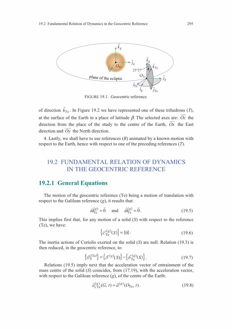
19.2 Fundamental Relation of Dynamics in the Geocentric Reference 295
FIGURE 19.1. Geocentric reference.
of direction Tek
. In Figure 19.2 we have represented one of these trihedrons (T),
at the surface of the Earth in a place of latitude β. The selected axes are: Oz
the
direction from the place of the study to the centre of the Earth, Ox
the East
direction and Oy
the North direction.
4. Lastly, we shall have to use references (R) animated by a known motion with
respect to the Earth, hence with respect to one of the preceding references (T).
19.2 FUNDAMENTAL RELATION OF DYNAMICS
IN THE GEOCENTRIC REFERENCE
19.2.1 General Equations
The motion of the geocentric reference (Te) being a motion of translation with
respect to the Galilean reference (g), it results that:
( ) ( )Te Te0 and 0g gω ω= = . (19.5)
This implies first that, for any motion of a solid (S) with respect to the reference
(Te), we have:
( )( ) Te 0
gS = . (19.6)
The inertia actions of Coriolis exerted on the solid (S) are null. Relation (19.3) is
then reduced, in the geocentric reference, to:
( ) ( ) ( )( ) TeTe( )
ggS S S= − . (19.7)
Relations (19.5) imply next that the acceleration vector of entrainment of the
mass centre of the solid (S) coincides, from (17.19), with the acceleration vector,
with respect to the Galilean reference (g), of the centre of the Earth:
( ) ( )
TeTe ( , ) ( , )g g
ea G t a O t=
. (19.8)
23°27'
OSo
gi
gj
gk
OTe
gi
gj
gk
Tek
Tei
Tej
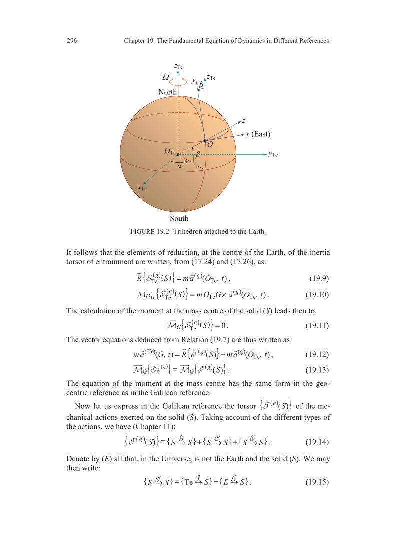
296 Chapter 19 The Fundamental Equation of Dynamics in Different References
FIGURE 19.2 Trihedron attached to the Earth.
It follows that the elements of reduction, at the centre of the Earth, of the inertia
torsor of entrainment are written, from (17.24) and (17.26), as:
( )( ) ( )TeTe ( , )
g gR S ma O t= , (19.9)
( )( ) Te
( )Te TeTe ( , )
g gO S m O G a O t= ×
. (19.10)
The calculation of the moment at the mass centre of the solid (S) leads then to:
( )( ) Te 0g
G S =
. (19.11)
The vector equations deduced from Relation (19.7) are thus written as:
( ) (Te) (g)
Te( , ) ( ) ( , )g
m a G t R S m a O t−= , (19.12)
( ) ( ) Te ( )g
G GS S=
. (19.13)
The equation of the moment at the mass centre has the same form in the geo-
centric reference as in the Galilean reference.
Now let us express in the Galilean reference the torsor ( ) ( )g
S of the me-
chanical actions exerted on the solid (S). Taking account of the different types of
the actions, we have (Chapter 11):
( ) ( )g S S SS S S S= + +→→ → . (19.14)
Denote by (E) all that, in the Universe, is not the Earth and the solid (S). We may
then write:
Te S E SS S = +→ →→ . (19.15)
zTe
North
South
x (East)
xTe
yTe
zTe y
OTe
Ω
z
O

19.2 Fundamental Relation of Dynamics in the Geocentric Reference 297
Moreover, the motion of the centre of the Earth, supposed to be submitted to the
only gravitational actions, is defined in the reference (g) by:
( )Te Te( , ) Te Te
gm a O t R= → , (19.16)
where mTe is the mass of the Earth and where the actions of gravitation are:
Te TeTe Te E S= +→ →→ . (19.17)
The actions of gravitation exerted by the solid (S) on the Earth are negligible
compared to the actions of gravitation exerted by (E). Whence:
TeTe Te E= →→ , (19.18)
and the vector equation (19.12) is written:
(Te)
Te
( , ) Te
.Te
m a G t R R R SS SS S
mR RE S E
m
= + + →→→
+ −→ →
(19.19)
The fundamental equations of dynamics, in the geocentric reference, are finally
given by Relations (19.19) for the resultant and (19.13) for the moment at the
mass centre of the solid. To apply Equation (19.19) of the resultant, it is then
necessary to consider specific assumptions adapted to each type of analysis.
19.2.2 Case of a Solid Located at the Vicinity of the Earth
For a solid located at the vicinity of the Earth, the model generally considered
consists first in neglecting the actions of gravitation other than the action of
gravitation exerted by the Sun, and next in neglecting the distance between the
centre of the Earth and the solid, compared to the distance between the centre of
the Earth and the centre of the Sun. The gravitational field is then constant over
the geometric domain constituted of the Earth and of its vicinity, this field being
the same one as that induced by the Sun at the centre of the Earth. Thus:
( ) ( ) ( )So TeTeG E G E S G O→ = → =
. (19.20)
It results that:
( )TeER m G OE S =→ , (19.21)
( )Te TeTe ER m G OE =→ , (19.22)
and Equation (19.19) is reduced to:
(Te)( , ) Tem a G t R R R SS SS S= + + →→→ . (19.23)
For a solid located at the vicinity of the Earth at the altitude h, the results
established in Chapter 12 (Subsection 12.1.4), show that the action of gravitation
298 Chapter 19 The Fundamental Equation of Dynamics in Different References
exerted by the Earth on the solid is a force whose the support passes through the
mass centre of the solid and whose the resultant is:
( )TeR mG h nS =→
, (19.24)
where ( )G h is the magnitude of the gravitational field induced by the Earth at the
altitude h, expressed by Relation (12.16), and n
is the unit vector of the direction
from the place where the solid is located to the centre of the Earth (Figure 12.3).
Finally, the fundamental relation of dynamics applied to the motion of the solid
(S) with respect to the geocentric reference (Te) is written in the form:
( ) ( ) Te Te ( )S S= , (19.25)
with
( ) Te ( ) TeS S S SS S+ += → →→ . (19.26)
19.3 FUNDAMENTAL RELATION OF DYNAMICS
IN A REFERENCE ATTACHED TO THE EARTH
19.3.1 Equations of Motion
Let (T) be a reference attached to the Earth and (Oxyz) the associated trihedron
(Figure 19.2). For a solid (S) located at the vicinity of the Earth, the fundamental
relation of dynamics (19.3) is written as:
( ) ( ) ( )T TS S= , (19.27)
with ( ) ( ) ( )( ) ( )( ) Te Te Te( ) ( )T
T TS S S S= − − . (19.28)
The torsors ( )( ) TeT S− and ( )( ) Te
T S− represent the inertia actions of entrain-
ment and of Coriolis which result from the motion of rotation of the Earth about
the axis of the poles. This motion of rotation is uniform, with a rotation vector
expressed in (18.56).
Inertia torsor of entrainment
The elements of reduction of the inertia torsor of entrainment at the mass centre
of the solid (S) are from (17.24), (17.26) and (18.56):
( )( ) ( )Te 2Te Te TeTR S m k k O GΩ= × ×
, (19.29)
( )( ) Te 2Te Te( )G T GS k S kΩ= ×
, (19.30)
where OTe is the centre of the Earth.

19.3 Fundamental Relation of Dynamics in a Reference Attached to the Earth 299
Inertia torsor of Coriolis
The elements of reduction are expressed from (17.30), (17.34) and (18.56) as:
( )( ) ( )TeTe2 ( , )T
TR S m k G tΩ= ×
, (19.31)
( )( ) ( ) ( )
TeTe Te2 ( ) 2 ( )T T
G T G S S GS I S k S kΩ ω Ωω= × + ×
. (19.32)
Equation (19.27) leads thus to the two vector equations:
( ) ( )
( )
2Te Te Te Te
( , ) Te
2 ( , ),
Tm a G t R R RS S SS S
m k k O G m k G tΩ Ω
= + +→ →→
− × × − ×
(19.33)
( )
( ) ( )
2Te Te
Te Te
( )
2 ( ) 2 ( ) .
TG G GS G
T TG S S G
k S kS SS S
I S k S k
Ω
Ω ω Ω ω
= + − ×→→
− × − ×
(19.34)
19.3.2 Action of Earthly Gravity
The action of gravity induced by the Earth was described in Section 12.2. We
then simply reported (Subsection 12.2.1) that this action resulted from the super-
position of the action of gravitation exerted by the Earth and the action generated
by the motion of the Earth about its South-North axis. We give now a more
precise definition of this action.
The action of gravity exerted by the Earth on a solid is the force whose the
support passes through the mass centre of the solid and whose the resultant is the
sum of the resultants of the action of gravitation induced by the Earth and of the
inertia action of entrainment.
The action of gravity is represented by a torsor which we denoted by e( )S .
From the preceding definition, we have:
( )
2Te Te Tee( ) ,Te
e( ) 0.G
R S R m k k O GS
S
Ω= − × ×→
=
(19.35)
The resultant of the action of gravity is thus written in the form:
e( )R S mg= , (19.36)
with
( )
2Te Te Teg G n k k O GΩ= − × ×
, (19.37)
where n
is the unit vector of the direction from the mass centre to the centre of
the Earth (Figure 19.3).
Express the vector g
as a function of the latitude β and of the longitude α of

300 Chapter 19 The Fundamental Equation of Dynamics in Different References
FIGURE 19.3. Direction at a point at the vicinity of the Earth.
the place where the solid is located (Figure 19.3). We have:
Te
Te
sin ( )cos ,
,
n k u
O G Rn
β α β = − +
=
(19.38)
where R is the distance from the mass centre to the centre of the Earth, practically
equal to the radius of the Earth when a solid is at the vicinity of the Earth. Thus, it
results that:
2 ( ) cosg G n R uΩ α β= +
. (19.39)
The numerical application of this expression shows that, in practice, g
differs
very little from G n
(Subsection 12.2.1).
19.3.3 Conclusions on the Equations of Dynamics in a Reference Attached to the Earth
Equation (19.33) of the resultant is written:
( )
( )
( )
Te
( , ) e( )
2 ( , ).
T TSR ma G t R S R R S SS S
m k G tΩ
= = + + →→
− ×
(19.40)
In a great number of problems, the term ( )
Te 2 ( , )m k G tΩ− × will have a negli-
gible influence.
yTe
North
South
xTe
zTe
OTe
G
Tek n
( )u α

19.4 Equations of Dynamics with respect to a Reference of Arbitrary Known Motion 301
With regard to Equation (19.34) of the moment at the mass centre:
— The term 2Te Te( )Gk S kΩ− ×
is null if the solid has a spherical symmetry.
In the other cases, this term is rather low so that it can be neglected being given
the value of Ω2.
— The two other terms in Ω will be with a less degree negligible in many
applications. We keep them in the expression of the moment for a later decision.
Thus:
( )
( ) ( ) Te Te 2 ( ) 2 ( ) .
TG G GS
T TG S S G
S SS S
I S k S kΩ ω Ω ω
= + →→
− × − ×
(19.41)
In all the analyses for which the terms in Ω can be neglected, it is said that the
Earth can be considered as a Galilean reference. On this assumption of “Galilean
Earth”, the fundamental equation of dynamics thus can be written:
( ) ( ) ( )T TS S= , (19.42)
with
( ) ( ) e( )T S S S SS S= + + →→ (19.43)
The exerted actions are reduced to the action of gravity induced by the Earth, to
the electromagnetic actions and to the actions of contact.
This model allows us to solve all the usual problems of engineering, for which
too high speeds do not occur.
19.4 EQUATIONS OF DYNAMICS OF A BODY WITH
RESPECT TO A REFERENCE WHOSE THE MOTION
IS KNOWN RELATIVELY TO THE EARTH
Let (R) be a reference of which the motion is known with respect to a reference
(T) attached to the Earth. This motion will be characterized by the kinematic
torsor, itself defined by its elements of reduction at a point OR of the reference (R):
( ) ( )
( ) ( )
,
( , ).R
T TR R
T TO R R
R
O t
ω=
=
(19.44)
The dynamic torsor relatively to the reference (R) of the solid (S) of which we
study the motion is:
( ) ( ) ( )( ) ( )( ) R T T TS S R RS S= − − . (19.45)
302 Chapter 19 The Fundamental Equation of Dynamics in Different References
And the fundamental equation of dynamics is written in the reference (R):
( ) ( ) ( )R RS S= , (19.46)
with
( ) ( ) ( )( ) ( )( ) ( ) ( )R T T TR RS S S S= − − . (19.47)
The torsors ( )( ) TR S− and ( )( ) T
R S− represent the inertia actions of entrain-
ment and Coriolis which result from the motion of the reference (R) with respect
to the Earth.
The vector equations of the motion with respect to the reference (R) are
deduced from Expression (19.46), while taking account of (19.40) or (19.41), and
from the expressions of the elements of reduction of the inertia torsors (Relations
(17.24) to (17.34)).
Thus, the equation of the resultant is written:
( ) ( )( , ) ( )R RSR m a G t R e S R R S SS S= = + + →→
( ) ( ) ( )( )( ) ( , )T T T TR R R R R Rm a O t O G O Gω ω ω − + × + × ∧
(19.48)
( ) ( ) ( )
Te 2 ( , ) ( , ) ,TRm k G t G tΩ ω − × + ×
with
( ) ( ) ( ) ( ) ( ) ( )
( , ) ( , )
( , ) ( , ) .
TG R
T TR R R
G t G t
G t O t O Gω
= +
= + + ×
(19.49)
In the same way, the equation of the moment is written in the form:
( ) RG G GS S SS S= + →→
( ) ( ) Te Te2 ( ) 2 ( )T T
G S S GI S k S kΩ ω Ω ω− × − ×
( ) ( ) ( )( ) ( )T T T
G R R G RS Sω ω ω− − ×
(19.50)
( ) ( ) ( ) ( )2 ( ) 2 ( ) .T R R T
G R S S G RI S Sω ω ω ω− × + ×
The two expressions of the resultant (19.48) and of the moment (19.50) have
complex general forms. In practice, they will not be used directly in these forms,
but they will be introduced simply when the relations of composition of motions
will be applied to the motions under consideration.
Comments 303
COMMENTS
In the preceding chapter, the fundamental principle of dynamics was
stated with respect to a Galilean reference of which the origin is the centre
of the Sun and directions are fixed relatively to fixed stars. In practice,
Engineer studies motions with respect to references attached to the Earth.
After having established the general equations of dynamics relatively to
a non Galilean reference, the present chapter derives the fundamental
relation of dynamics in a reference attached to the Earth. The reader will be
interested in the development of the process and will retain the result: the
fundamental equation of dynamics in a reference attached to the Earth has
the same form as the fundamental equation in a Galilean reference, the
exerted mechanical actions being reduced to the action of gravity, the
electromagnetic actions and the actions of contact. The action of gravity
induced by the Earth which was introduced in Chapter 12 is entirely
characterized in the present chapter.

CHAPTER 20
General Process for Analysing a Problem of Dynamics of Rigid Bodies
In this chapter, we study the problem of the dynamics of a rigid body or a set of
rigid bodies. In practice, the results which will be derived in Galilean reference
can be applied to a reference attached to the Earth provided that the induced velo-
cities are not too high (Subsection 19.3.3). This type of reference will be called as
pseudo-Galilean reference
20.1 DYNAMICS OF RIGID BODY
20.1.1 General Equations
We consider a solid (S) in motion with respect to a Galilean (or pseudo-
Galilean) reference (g). Among the mechanical actions exerted on the solid, we
distinguish, as in Subsection 14.2.1, between:
— The known actions which can be calculated: actions of gravitation, of gravity,
electromagnetic actions. The whole of the actions of this type exerted on the solid
(S) and measured in the Galilean reference (g) are represented by the torsor
denoted by ( ) S .
— The actions induced by the connections (or actions of contact) which are
represented by the torsor S S→
, which we shall denote by ( ) S .
In order to simplify the notations, we denoted by ( ) S and ( ) S , instead
of ( )( ) gS of ( )( ) ,g S the torsors of the actions expressed in the reference (g).
Contrary to the actions of the first type, the actions induced by the connections
are not known a priori. Their determination is part of the problem to be solved. In
order to completely determine the problem of the dynamics of the solid (S), it will
20.1 Dynamics of Rigid Body 305
be necessary to make assumptions on the physical nature of the connections:
perfect connections, connections with viscous friction or connections with dry
friction. The validity of these assumptions will be deduced a posteriori, by con-
fronting the experimental observations with the theoretical results derived starting
from these assumptions.
The equation of dynamics is thus written in the Galilean reference (g) in the
form: ( ) ( ) ( ) g
S S S= + . (20.1)
If m and G are respectively the mass and the mass centre of the solid, the prece-
ding equation leads to the two vector equations of the dynamics of the solid.
Equation of the resultant( ) ( ) ( ) ( ) ( , )g T
SR ma G t R S R S= = + . (20.2)
Equation of the moment at a point P
( ) ( ) ( ) gP P PS S S= +
. (20.3)
Let us recall (Section 16.3) that we have:
( ) ( ) ( ) ( ) ( ) ( ) ( ) ( , )
g g g ggP P PS S S Sm PG a P t S Sω ω ω= × + + ×
, (20.4)
and that this expression is simplified when the point P coincides with the mass
centre: ( ) ( ) ( ) ( ) ( ) ( )g g g g
G G GS S S SS Sω ω ω= + × . (20.5)
By choosing an orthonormal basis ( )1 2 3, , u u u
to express the equation of the
resultant and an orthonormal basis ( )1 2 3, , v v v
to express the equation of the
moment at the point P, the vector equations (20.2) and (20.3) lead to 6 scalar
equations. The choices of the point P and of the bases (identical or not) will be
carried out so as to simplify as well as possible the writing of these equations.
In some cases, the theorem of power-energy could be useful. It will then be
written as:
( ) ( ) ( ) ( ) ( ) cd
d
g g gE P S P S
t= + . (20.6)
It does not bring however any new information with respect to the preceding
scalar equations.
20.1.2 General Process of Analysis
The general process for analysing a problem of dynamics of a solid consists to
establish Equation (20.1) of the dynamics. This analysis will be implemented in
the following way.
1. Choose a Galilean (or pseudo-Galilean) reference. For Engineer, this refe-
rence will be generally a reference attached to the Earth.

306 Chapter 20 General Process for Analysing a Problem of Dynamics of Rigid Bodies
2. Find the parameters of situation relative to the motion of the body with
respect to the reference system, taking into account the connections.
3. Implement the kinematic analysis: determine the kinematic torsor; the
conditions of sliding and non-sliding if necessary; the velocity and acceleration
vectors of the mass centre of the body.
4. Implement the kinetic analysis: determine the kinetic torsor, the dynamic
torsor, the kinetic energy, relatively to the motion of the body with respect to the
reference system.
5. Analyse the mechanical actions exerted on the body: torsors representing
these actions, powers developed by these actions. Examine the assumption of
perfect connections.
6. Apply the fundamental principle of dynamics, which leads to six scalar
equations.
6'. In some cases, applying the theorem of power-energy could provide a scalar
equation apt to replace one of the six preceding equations judiciously.
7. To solve the problem of dynamics, it will be then necessary to introduce
assumptions on the physical nature of the connections: perfect connections, con-
nections with viscous or dry friction. These assumptions will lead to additional
scalar equations.
8. Solving the system constituted of the six scalar equations derived from the
fundamental principle and of equations deduced from the assumptions on the phy-
sical nature of connections will then make it possible to find:
— the equations of motion: parameters of situation as a function of time;
— the components of the actions induced by the connections, on which no
assumption will have been considered previously.
20.2 DYNAMICS OF A SET OF BODIES
We consider a set (D) constituted of n solids: (S1), (S2), ..., (Si), ..., (Sj), ..., (Sn).
The mechanical actions which are exerted have been considered in Subsection
14.2.2, in the context of the analysis of the equilibrium of this set of solids. The
actions were then divided into internal actions and external actions. We keep the
notations used in this subsection.
The equation of dynamics applied to the motion of each solid with respect to
the Galilean reference (g) is written:
( ) ( ) ( ) ( ) ( )
1
1, 2, . . . , ,
i
ng
i i j i j iS
ji
S S S S
i n
=≠
= + + +
=
(20.7)
where ( ) i
g
S is the dynamic torsor relatively to the motion of the solid (Si) with
respect to the reference (g).
20.3 Conclusion 307
Equation (20.7) leads to 6 scalar equations for each solid, thus a total of 6n
scalar equations for the set (D).
Other equations with different forms, but depending on the preceding
equations, can be obtained by applying the fundamental principle to any part of
the set (D). This can be applied to the set (D) itself, which leads to:
( ) ( ) ( ) 1
ng
i iD
i
D D S S
=
= → = + , (20.8)
with
( ) ( ) 1
i
ng g
D S
i=
= . (20.9)
Relation (20.8) leads to the elimination of the actions internal to the set (D). This
property is general: the application of the fundamental principle of dynamics to
any part of the set (D) leads to a relation, where the mechanical actions internal to
this part are excluded.
As in the case of one solid, it is necessary to introduce assumptions on the
physical nature of the internal and external connections. These assumptions
associated to Relations (20.7), or to linear combinations, will then make it
possible to solve the problem of dynamics of the set of rigid bodies, by deriving
the equations of motion and characterizing the actions induced by the connections.
20.3 CONCLUSION
The general unity of the development implemented in the present textbook has
consisted in setting up gradually the different concepts necessary to analyse a
problem of mechanics (dynamics or statics) of a rigid body or a set of rigid
bodies. This development finds its conclusion in this chapter. Its objective was to
lay the foundations of a general and systematic process for analysing a problem of
mechanics. The issue of this development shows that actually there exists only
one problem of mechanics, of which the analysis is implemented for each solid
according the general process of analysis reported in Subsection 20.1.2. Each
problem differs by the mechanical system to analyse and the particular points of
interest of Engineer, associated to each problem. In fact, once the mechanical
system is given, the problem is entirely stated and the process of analysis is
determined.
308 Chapter 20 General Process for Analysing a Problem of Dynamics of Rigid Bodies
COMMENTS
The chapter develops the general process for analysing a problem of
dynamics of a rigid body. This analysis is always implemented in the same
way: 1) choose a reference system, 2) derive the parameters of situation, 3)
implement the kinematic analysis, 4) implement the kinetic analysis, 5)
analyse the mechanical actions, 6) apply the fundamental principle of
dynamics.
Then, solving the equations of the problem of dynamics requires to
introduce assumptions on the physical nature of the connections: con-
nections without friction, connections with viscous friction or connections
with dry friction. Next, solving the equations deduced from the funda-
mental principle and associated to the equations on the physical nature of
the connections allows us to derive the equations of motion and to charac-
terize the actions induced by the connections.
For a set of rigid bodies, the preceding process is applied to each body of
the set.
In practice, all the problems of mechanics will be analysed using this
same process.
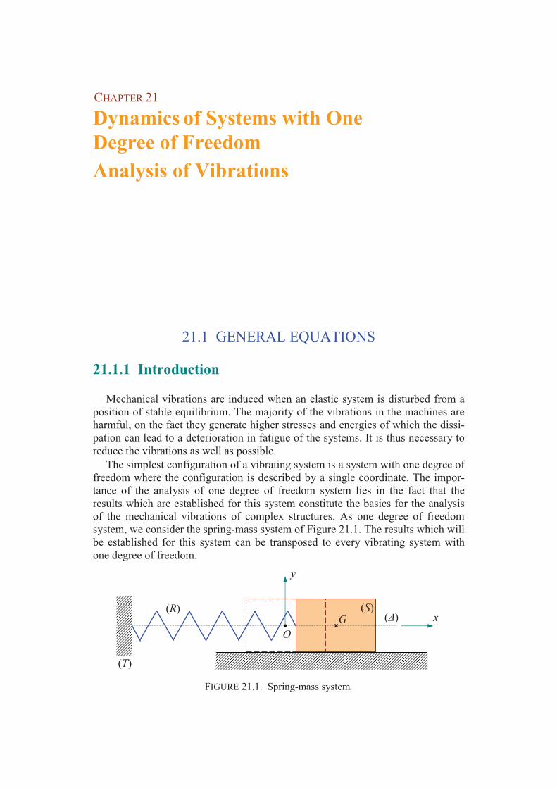
CHAPTER 21
Dynamics of Systems with One Degree of FreedomAnalysis of Vibrations
21.1 GENERAL EQUATIONS
21.1.1 Introduction
Mechanical vibrations are induced when an elastic system is disturbed from a
position of stable equilibrium. The majority of the vibrations in the machines are
harmful, on the fact they generate higher stresses and energies of which the dissi-
pation can lead to a deterioration in fatigue of the systems. It is thus necessary to
reduce the vibrations as well as possible.
The simplest configuration of a vibrating system is a system with one degree of
freedom where the configuration is described by a single coordinate. The impor-
tance of the analysis of one degree of freedom system lies in the fact that the
results which are established for this system constitute the basics for the analysis
of the mechanical vibrations of complex structures. As one degree of freedom
system, we consider the spring-mass system of Figure 21.1. The results which will
be established for this system can be transposed to every vibrating system with
one degree of freedom.
FIGURE 21.1. Spring-mass system.
(T)
(R) (S) ()
O
G x
y
310 Chapter 21 Dynamics of Systems with One Degree of Freedom. Analysis of Vibrations
The spring-mass system is constituted of a solid (S) linked to a support (T)
through an elastic spring (R). Moreover, the solid is connected to the support by a
prismatic connection of horizontal axis (∆), also axis of the spring. It results that
horizontal displacement of the mass centre G of the solid is possible only along
the axis (∆).
21.1.2 Parameters of Situation
We choose the coordinate system (Oxyz) attached to the support (T) in such a
way that the axis Ox
coincides with the axis (∆), that the point O coincides with
the equilibrium position of the mass G (in the case where there is no friction) and
that the axis Oy
is upward vertical. The orientation of the solid (S) does not
change during the motion, so the motion has one parameter of situation, the
abscissa x of the point G along the axis Ox
: OG x i=
.
21.1.3 Kinematics
The elements of reduction at the mass centre G of the kinematic torsor ( ) TS
are: ( ) ( )
( ) ( )
0,
( , ) .
T TS S
T TG S
R
G t x i
ω= =
= =
(21.1)
All the points of the solid have the same velocity vector and the same acceleration
vector: ( )
( , )Ta G t x i= . (21.2)
21.1.4 Kinetics
The elements of reduction at the mass centre G of the kinetic torsor are:
( ) ( )
( ) ( )
( , ) ,
( ) 0.
T TS
T TG S G S
R m G t mx i
S ω
= =
= =
(21.3)
In the same way, the elements of reduction of the dynamic torsor are:
( ) ( )
( ) ( ) ( ) ( )
( , ) ,
( ) ( ) 0.
T TS
T T T TG S G S S G S
R ma G t mx i
S Sω ω ω
= =
= + × =
(21.4)
Lastly, the kinetic energy is:
( ) ( ) ( ) 2c
1 1( )
2 2T T T
S SE S mx= =⋅ . (21.5)

21.2 Vibrations without Friction 311
21.1.5 Mechanical Actions Exerted on the Solid
The mechanical actions exerted on the solid are reduced to the action of gra-
vity, the action of the spring and the action of the support induced by the prismatic
connection.
1. Action of gravity
The action is represented by the torsor e( )S of which the elements of reduc-
tion at the mass centre are:
e( ) ,
e( ) 0.G
R S mg j
S
= −
=
(21.6)
The power developed by the action of gravity is:
( ) ( ) e( ) e( ) 0T TSP S S= =⋅ . (21.7)
2. Action of the spring
The action exerted by the spring is a force of which the support is the axis of
the spring. The action is represented by the torsor ( )S of which the elements
of reduction at G are:
( ) ,
( ) 0,G
R S kx i
S
= −
=
(21.8)
where k is the constant of rigidity or the stiffness of the spring.
The power developed by the action of the spring is:
( ) ( ) ( ) ( )T TSP S S k x x= = −⋅ . (21.9)
3. Action of the support induced by the prismatic connection
The action of connection exerted by the support is represented by the torsor
( )S of which the elements of reduction at the point G are:
( ) ,
( ) .
l l l
G l l l
R S X i Y j Z k
S L i M j N k
= + +
= + +
(21.10)
The components Xl, Yl, ..., Nl, of the action of connection are to be determined.
The power developed by the action of connection is:
( ) ( ) ( ) ( )T TlSP S S X x= =⋅ . (21.11)
21.1.6 Application of the Fundamental Principle
In the case where the support is a pseudo-Galilean reference (attached to the
Earth), the fundamental principle applied to the spring-mass system is written:
312 Chapter 21 Dynamics of Systems with One Degree of Freedom. Analysis of Vibrations
( ) e( ) ( ) ( )TS S S S= + + . (21.12)
This equation leads to two vector equations, the equation of the resultant and the
equation of the moment at the point G:
( ) e( ) ( ) ( )TSR R S R S R S= + +
, (21.13)
( ) e( ) ( ) ( )TG G G GS S S S= + +
. (21.14)
From these equations, we deduce the 6 scalar equations:
,
0 ,
0 ,
0 ,
0 ,
0 .
l
l
l
l
l
l
mx k x X
mg Y
Z
L
M
N
= − +
= − +
=
=
=
=
(21.15)
The theorem of power-energy:
( ) ( ) ( ) ( ) cd
e( ) ( ) ( )d
T T T TE P S P S P St
= + + (21.16)
leads to the equation:
lmxx kxx X x= − + . (21.17)
We find the first of Equations (21.15) again.
Finally, we obtain 6 equations for 7 unknowns: Xl, Yl, Zl, Ll, Ml, Nl, x. An
additional equation will be derived from the physical nature of the connection.
The problem could then be entirely determined.
In fact, five equations of the system (21.15) are already solved:
lY mg= , (21.18)
0lZ = , (21.19)
( ) 0G S =
. (21.20)
It results that the action of connection is a force of which the support passes
through the mass centre G.
It remains to solve the first equation of (21.15):
lmx k x X= − + . (21.21)
The hypothesis on the physical nature of the connection will allows us to express
the component Xl. Next, solving (21.21) will lead to the expression of the motion
x as a function of time. Equation (21.21) is called the equation of motion.
We observe that, in the case of this spring-mass system, the theorem of power-
energy leads to the equation of motion.

21.2 Vibrations without Friction 313
21.2 VIBRATIONS WITHOUT FRICTION
21.2.1 Equation of Motion
In the case where the connection is without friction (perfect connection), the
power developed by the action of connection is zero. Thus from (21.11):
0lX = . (21.22)
The equation of motion is reduced to:
mx k x= − . (21.23)
This equation can be written in the reduced form:
20 0x xω+ = , (21.24)
introducing:
20
k
mω = . (21.25)
The quantity 0ω is the natural angular frequency of the spring-mass system
without friction.
21.2.2 Free Vibrations
The free vibrations are the vibrations which are observed when the solid (S) is
displaced from its equilibrium position and released. These vibrations are solu-
tions of Equation (21.24). This equation is satisfied by:
1 0cosx C tω= and 2 0sinx C tω= ,
where C1 and C2 are arbitrary constants. By addition of these solutions, we obtain
the general solution of equation of motion (21.24). Hence:
1 0 2 0cos sinx C t C tω ω= + . (21.26)
The vibratory motion represented by this equation is a simple harmonic
motion, where the constants C1 and C2 are deduced from the initial conditions.
We consider that, at the initial instant ( 0)t = , the solid has a displacement x0 from
its equilibrium, then the solid is released with a velocity 0x . By substituting 0t =
into Equation (21.26), we obtain:
1 0C x= . (21.27)
Deriving Equation (21.26) with respect to time, then substituting 0t = , we have:
02
0
xC
ω=
. (21.28)
Thus, the expression of the free vibrations of the solid (S) is written:
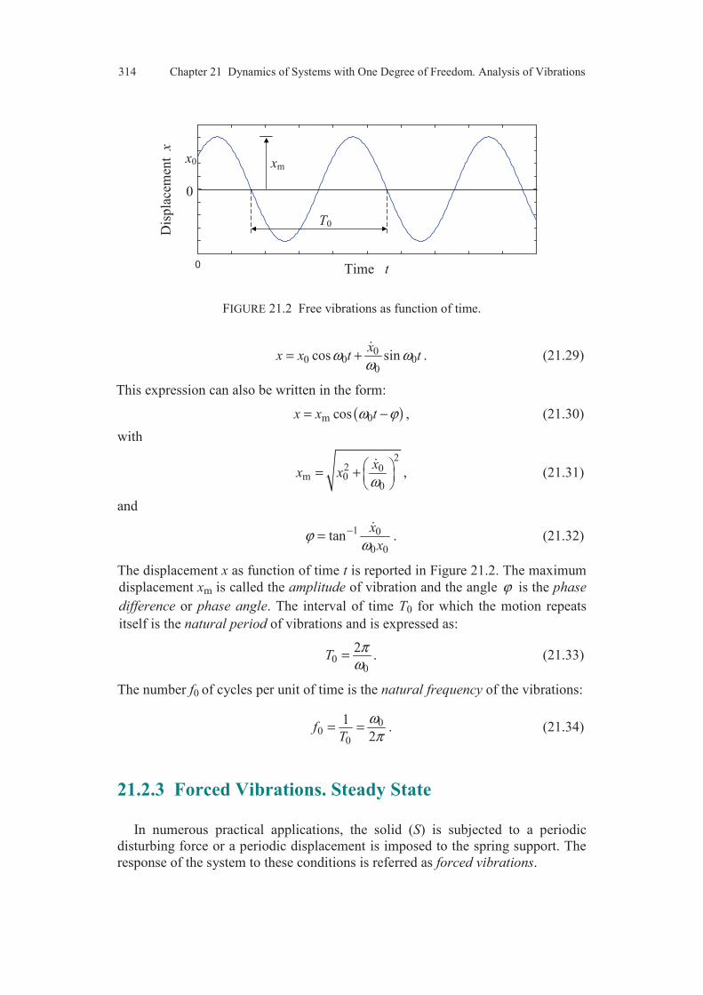
314 Chapter 21 Dynamics of Systems with One Degree of Freedom. Analysis of Vibrations
FIGURE 21.2 Free vibrations as function of time.
00 0 0
0
cos sinx
x x t tω ωω
= +
. (21.29)
This expression can also be written in the form:
( )m 0cosx x tω ϕ= − , (21.30)
with
22 0
m 00
xx x
ω = +
, (21.31)
and
1 0
0 0
tanx
xϕ
ω−=
. (21.32)
The displacement x as function of time t is reported in Figure 21.2. The maximum
displacement xm is called the amplitude of vibration and the angle ϕ is the phase
difference or phase angle. The interval of time T0 for which the motion repeats
itself is the natural period of vibrations and is expressed as:
00
2T
πω
= . (21.33)
The number f0 of cycles per unit of time is the natural frequency of the vibrations:
00
0
1
2f
T
ωπ
= = . (21.34)
21.2.3 Forced Vibrations. Steady State
In numerous practical applications, the solid (S) is subjected to a periodic
disturbing force or a periodic displacement is imposed to the spring support. The
response of the system to these conditions is referred as forced vibrations.
0
-0.00
Time t
Dis
pla
cem
ent
x
x0 xm
T0

21.2 Vibrations without Friction 315
We consider the case where the solid (S) of the spring-mass system of Figure
21.1 is subjected to a periodic force f of horizontal component m sinf tω . The
term m sinf tω is called a harmonic forcing function. The equation of motion
(21.23) without friction is then written as:
m sinmx kx f tω= − + . (21.35)
This equation is rewritten in the reduced form as:
20 m sinx x q tω ω+ = , (21.36)
with
mm
fq
m= . (21.37)
A particular solution of Equation (21.36) is:
3 sinx C tω= , (21.38)
where C3 is a constant which must satisfy Equation (21.36). We obtain:
3 2 20
mqC
ω ω=
−. (21.39)
Thus, the particular solution is given by:
2 20
sinmqx tω
ω ω=
−. (21.40)
The general solution of Equation (21.36) is obtained by adding this particular
solution to the general solution (2.7) of the free vibrations. We obtain:
1 0 2 0 2 20
cos sin sinmqx C t C t tω ω ω
ω ω= + +
−. (21.41)
The first two terms of this expression represent the free vibrations which were
considered previously. These free vibrations are also called transient vibrations
since in the practice these vibrations are rapidly damped by the damping forces
(Subsection 21.3.3.1). The third term, depending on the disturbing force, repre-
sents the forced vibrations of the system, obtained in the steady state. These
forced vibrations have the same period 2 /T π ω= as that of the disturbing force.
They can be expressed as:
m2 2 20 0
1sin
1 /
qx tω
ω ω ω=
−. (21.42)
The factor 2m 0/q ω is the displacement that the disturbing force qm would produce
if it was acting as a static force. The term ( )2 201/ 1 /ω ω− accounts for the dyna-
mical effect of the disturbing force. Its absolute value:
2 20
1( )
1 /K ω
ω ω=
−, (21.43)
is usually called the magnification factor. It depends only of the frequency ratio

316 Chapter 21 Dynamics of Systems with One Degree of Freedom. Analysis of Vibrations
FIGURE 21.3 Variation of the magnification factor as a function of the frequency.
0/ω ω , ratio of the frequency of the disturbing force to the natural frequency of the
system. The variation of the magnification factor is plotted against the frequency
ratio in Figure 21.3.
When the frequency of the disturbing force is small in comparison with the
frequency of the free vibrations, the magnification factor is approximately equal to
1. The displacements are about the same as in the case of a static disturbing force.
When the frequency of the disturbing force approaches the natural frequency of
the system, the magnification factor and thus the amplitude of the forced vibra-
tions rapidly increase and become infinite when the force frequency exactly coin-
cides with the natural frequency. The system is subjected to the resonance. In
practice, there is a dissipation of energy due to damping and the amplitude of the
vibrations is limited by the damping effects (Section 21.3). However, the system
should not be excited near its natural frequency.
When the frequency of the disturbing force increases beyond the natural
frequency, the magnification factor decreases and approaches zero for high values
of the frequency. The system may be considered as remaining stationary.
Considering the sign of the expression ( )2 201/ 1 /ω ω− , it is observed that for the
case where 0ω ω< this expression is positive. The displacement of the vibrating
mass has the same sign as that of the disturbing force. The vibrations are in phase
with the excitation. In the case where 0ω ω> , the expression is negative and the
displacement of the mass is in the direction opposite to that of the force. The
vibrations are out of phase.
In what precedes, we have considered the case of an excitation of the system by
an imposed force. It is also possible to produce forced vibrations by imposing a
displacement to the end support of the spring (Figure 21.4). In the case of a
harmonic displacement, the support displacement is:
m sins sx x tω= , (21.44)
where xs is the displacement of the support from the equilibrium position. The
displacement of the solid (S) referred to the support (T) is given by:
s rx x x= + , (21.45)
0.0 0.5 1.0 1.5 2.0 2.5 3.00
1
2
3
4
Frequency 0/ω ω
Magn
ific
ation f
acto
r K

21.2 Vibrations without Friction 317
FIGURE 21.4. Displacement imposed to the spring end.
introducing the displacement xr referred to the end support of the spring. The
resultant of the force exerted by the spring is transposed of (21.8). Thus:
( ) rR S k x i= − , (21.46)
and the equation of motion (21.23) is modified as:
rmx k x= − . (21.47)
This equation leads to the motion equation of forced vibrations:
m sinsmx k x k x tω+ = − . (21.48)
This motion equation can be written in the reduced form (21.36), setting:
2m m 0 ms s s
kq x x
mω= = . (21.49)
The motion equation is reduced to the case of a disturbing force.
In some other applications, it is more interesting to consider the case where an
acceleration is imposed to the support. The system spring-mass is then used as
accelerometer, device used to measure the acceleration of the support. In the case
of a harmonic acceleration, we have:
m sinsx a tω= . (21.50)
Considering Relations (21.45) and (21.47), the equation of motion is written in the
form:
s r rmx mx k x+ = − ,
or
m sinr rmx kx ma tω+ = − . (21.51)
Hence, the reduced form of motion equation:
20 m sinr rx x q tω ω+ = , (21.52)
setting
m mq a= − . (21.53)
Again, the motion equation is reduced to the form (21.36) of an imposed force.
y
(T)
(R) (S) ()
O
G x
xs x

318 Chapter 21 Dynamics of Systems with One Degree of Freedom. Analysis of Vibrations
However, it must be noted that Equation (21.52) is the motion equation expres-
sed in the relative reference associated to the end support of the spring. The forced
vibrations in this reference are transposed from Equation (21.42):
m2 2 20 0
1sin
1 /r
ax tω
ω ω ω= −
−(21.54)
21.3 VIBRATIONS WITH VISCOUS DAMPING
21.3.1 Equation of Motion with Viscous Damping
In previous discussions we did not consider the effects of dissipative forces. In
practice, it is necessary to take into consideration the damping forces which may
arise from several different sources, such as friction between dry sliding surfaces,
friction between lubricated surfaces, air or fluid resistance, internal friction due to
imperfect elasticity of materials, etc. Among all these processes of energy dissi-
pation, the simplest case to deal with mathematically is the case where the
damping force is proportional to the velocity. This damping process is called
viscous damping. The damping processes of complex types are generally re-
placed, for the purpose of the analyses, by an equivalent viscous damping. This
equivalent damping is determined in such a way as to produce the same dissi-
pation of energy by cycle as that produced by the actual damping processes
(Section 21.5).
In the case of a viscous damping of the spring-mass system of Figure 21.1, the
component Xl of connection introduced in (21.10) is opposed to the component x
of the velocity. Hence:
lX cx= − . (21.55)
The coefficient c is the coefficient of viscous damping. The motion equation
(21.21) is then written:
0mx cx k x+ + = . (21.56)
This equation can be rewritten in the reduced form:
202 0x x xδ ω+ + = , (21.57)
setting:
2
c
mδ = . (21.58)
The parameter δ is the damping coefficient. Equation (21.57) is the general reduced
form of the vibrations of a one degree of freedom system with viscous damping.
21.3.2 Free Vibrations
21.3.2.1 Introduction
To solve Equation (21.57) of the free vibrations, we use the usual method for
21.3 Vibrations with Viscous Friction 319
solving the linear differential equations, by searching a solution of the form:
rtx Ce= , (21.59)
where r is a parameter determined by reporting Expression (21.59) into Equation
(21.57). Thus, we obtain the characteristic equation:
2 202 0r rδ ω+ + = . (21.60)
The solutions of this equation are:
1,2r δ ∆′= − ± , (21.61)
where ∆′ is the reduced discriminant of the characteristic equation:
2 20∆ δ ω′ = − . (21.62)
The final form of the solution of Equation (21.57) depends on the sign of ∆′ .
21.3.2.2 Case of Low Damping
In the case of low damping such as:
0δ ω< , (21.63)
the term ∆′ is negative and Equation (21.60) has two conjugated complex roots:
2
1,2 0 20
1r iδδ ωω
= − ± − . (21.64)
These two roots can be put in the form:
1,2 dr iδ ω= − ± , (21.65)
introducing the angular frequency:
2
0 20
1dδω ωω
= − . (21.66)
It is usual to introduce the viscous damping ratio ξ, defined as:
00
or δξ δ ξω
ω= = . (21.67)
It results that:
20 1dω ω ξ= − , (21.68)
and the two roots (21.65) are expressed as:
21,2 0 0 1r iξ ω ω ξ=− ± − . (21.69)
Finally, Equation (21.57) of the free vibrations can be written in the form:
320 Chapter 21 Dynamics of Systems with One Degree of Freedom. Analysis of Vibrations
20 02 0x x xξω ω+ + = . (21.70)
The two complex roots (21.65) are thus given by:
1 2, .d dr i r iδ ω δ ω= − + = − − (21.71)
or from (21.69):
( ) ( )2 21 0 2 01 , 1 r i r iω ξ ξ ω ξ ξ= − + − = − − − . (21.72)
Substituting these roots into Expression (21.59), we obtain two solutions of Equa-
tion (21.57) or (21.70). Any linear combination of these solutions is also a
solution. For example:
( )
( )
1 2
1 2
11 1
12 2
cos ,2
sin .2
r t r t td
r t r t td
Cx e e C e t
Cx e e C e t
i
δ
δ
ω
ω
−
−
= + =
= − =
Adding these solutions, we obtain the general solution of Equation (21.57) or
(21.70) in the form:
( )1 2cos sintd dx e C t C tδ ω ω−= + , (21.73)
where C1 and C2 are constants which are determined from the initial conditions.
The factor te δ− in Solution (21.73) decreases with time, and the vibrations
generated by the initial conditions are gradually damped out.
The expression between brackets in Equation (21.73) is of the same form that
the one obtained in the case of vibrations without damping (21.26). It represents a
harmonic function of angular frequency given by Equation (21.66) or (21.68).
This frequency is called the angular frequency of the damped vibrations. The
variation 0/dω ω of this frequency referred to the natural frequency of the free
undamped vibrations is plotted in Figure 21.5 as a function of the damping ratio
0/ξ δ ω= . From this figure, it is observed that the frequency of the damped vibra-
tions is close to the frequency of undamped vibrations, even for notable value of
the damping ratio. For 0.1ξ = , the damped frequency is 00.995dω ω= ; for
0.2ξ = , the frequency is equal to 00.98ω and for 0.3ξ = , the damped frequency
is still 00.95 .ωConstants C1 and C2 in Expression (2.56) are deduced from the initial condi-
tions at time 0t = : the solid is displaced from its equilibrium position by a displa-
cement x0 and the solid is released with a velocity 0x . Thus, reporting these initial
conditions into Equation (21.73) and into the expression of the derivative of the
displacement with respect to time, we obtain:
0 01 0 2,
d
x xC x C
δω+
= =
. (21.74)
Thus, the motion of damped free vibrations of a one degree of freedom system is:
0 00 cos sint
d dd
x xx e x t tδ δ
ω ωω
− + = +
. (21.75)

21.3 Vibrations with Viscous Friction 321
FIGURE 21.5. Frequency variation as a function of damping.
This expression can be rewritten in the form:
( )m costdx x e tδ ω ϕ−= − , (21.76)
expression in which the maximum value is:
( )22 2 2 0 0
m 1 2 0 2d
x xx C C x
δ
ω
+= + = +
, (21.77)
and the phase angle is given by:
1 1 0 01
2 0
tan tand
x xC
C x
δϕ
ω− − + = =
. (21.78)
Expression (21.76) may be considered as representing a pseudo-harmonic motion,
having an exponentially decreasing amplitude mtx e δ− , a phase angle ϕ and a
pseudo-period:
2d
d
Tπ
ω= . (21.79)
The graph of the motion is plotted in Figure 21.6. The displacement-time curve is
tangent to the envelopes mtx e δ−± at the points m1, 1m′ , m2, 2m′ , etc., at instants
separated by the time interval /2dT . Because the tangents at these points are not
horizontal, the points of tangency do not coincide with the points of extreme
displacements from the equilibrium position. If the damping ratio is low, the
difference in these points may be neglected. For any damping, the time interval
between two consecutive extreme positions is however equal to half the pseudo-
period. Indeed, the velocity of the vibrating solid is derived from (21.76) as:
( ) ( )m mcos sint td d dx x e t x e tδ δδ ω ϕ ω ω ϕ− −= − − − − . (21.80)
The velocity is equal to zero when:
( )tan dd
tδω ϕ
ω− = − , (21.81)
damping ξ 1 0 0
1
dfr
eq
uen
cy
ω

322 Chapter 21 Dynamics of Systems with One Degree of Freedom. Analysis of Vibrations
FIGURE 21.6 Pseudo-harmonic motion.
which leads effectively to / /2d dt Tπ ω= = .
The ratio between two successive amplitudes mix and m 1ix + is:
( )m m
m 1 m
id
i d
tTi
t Ti
x x ee
x x e
δδ
δ
−
− ++
= = . (21.82)
The quantity l dTδ δ= is the logarithmic decrement. It is given by:
m
m 1 0
2 2ln i
l di d
xT
x
πδ πδδ δω ω+
= = = ≈ . (21.83)
This equation can be used for an experimental determination of the damping coef-
ficient δ. However, a greater accuracy is obtained by measuring the extreme am-
plitudes separated by n pseudo-cycles. In this case we have:
m
m
dn Ti
i n
xe
xδ
+= , (21.84)
and the logarithmic decrement is obtained as:
m
m
1ln i
li n
x
n xδ
+= . (21.85)
21.3.2.3 Case of High Damping
In the case of high damping such as:
0δ ω> , (21.86)
the term ∆′ is positive and the characteristic equation (21.60) has two roots r1 and
r2 which are real and negative. The general solution of the motion equation
(21.57) is:
0
0
m1
m2
m3 m4
1m′
2m′3m′
/ dϕ ω
m3xm4x
m1x
m2x
dT
mx
0x
0
Time t
Dis
pla
cem
ent
x
tmx e δ−
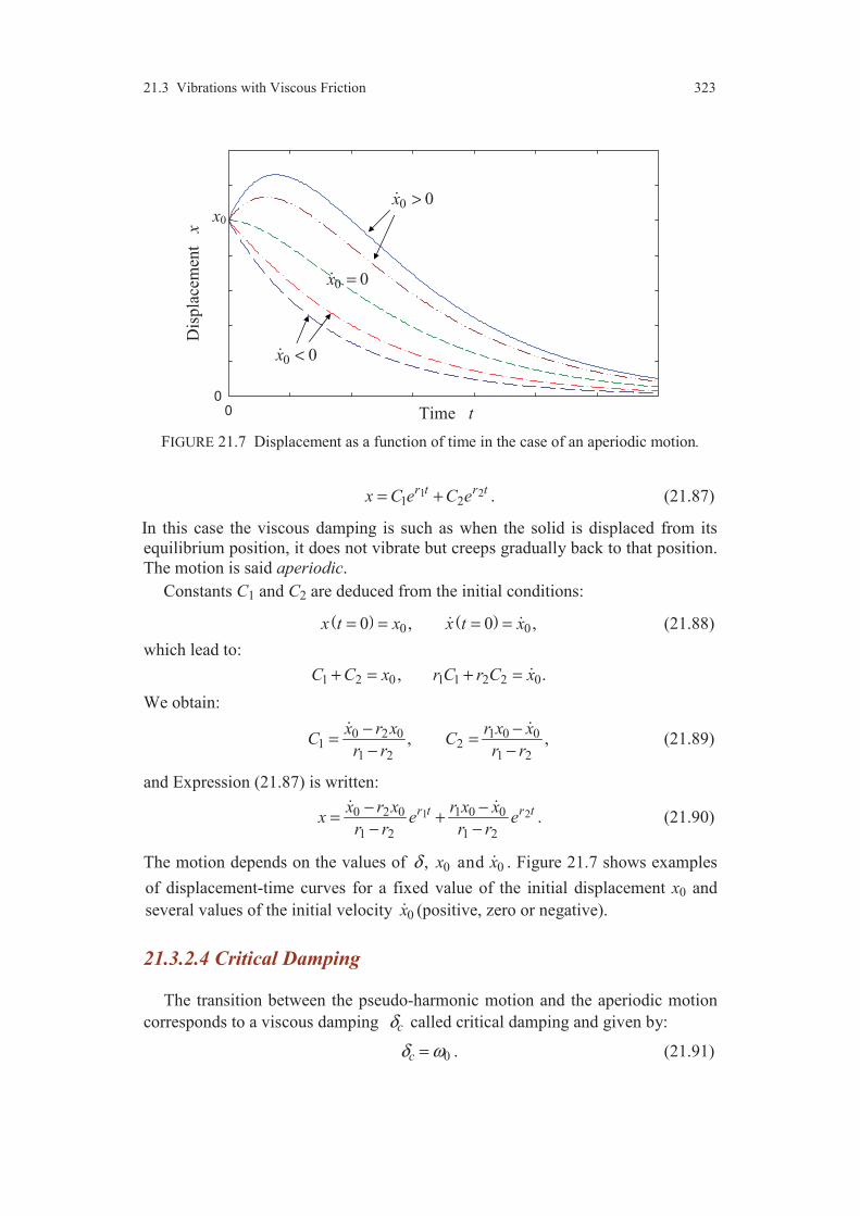
21.3 Vibrations with Viscous Friction 323
FIGURE 21.7 Displacement as a function of time in the case of an aperiodic motion.
1 21 2
r t r tx C e C e= + . (21.87)
In this case the viscous damping is such as when the solid is displaced from its
equilibrium position, it does not vibrate but creeps gradually back to that position.
The motion is said aperiodic.
Constants C1 and C2 are deduced from the initial conditions:
( ) ( )0 00 , 0 ,x t x x t x= = = = (21.88)
which lead to:
1 2 0 1 1 2 2 0, .C C x r C r C x+ = + =
We obtain:
0 2 0 1 0 01 2
1 2 1 2
, ,x r x r x x
C Cr r r r
− −= =
− −
(21.89)
and Expression (21.87) is written:
1 20 2 0 1 0 0
1 2 1 2
r t r tx r x r x xx e e
r r r r
− −= +
− −
. (21.90)
The motion depends on the values of 0 0, and x xδ . Figure 21.7 shows examples
of displacement-time curves for a fixed value of the initial displacement x0 and
several values of the initial velocity 0x (positive, zero or negative).
21.3.2.4 Critical Damping
The transition between the pseudo-harmonic motion and the aperiodic motion
corresponds to a viscous damping cδ called critical damping and given by:
0cδ ω= . (21.91)
00
Time t
Dis
pla
cem
ent
x
x0
0 0x >
0 0x =
0 0x <
324 Chapter 21 Dynamics of Systems with One Degree of Freedom. Analysis of Vibrations
In this particular case, the characteristic equation (21.60) has a double root:
1 2 0r r ω= = − , (21.92)
and the solution of the motion equation is:
( ) 01 2
tx C C t e ω−= + . (21.93)
Taking the initial conditions into account, we obtain:
1 0 2 0 0 0, ,C x C x xω= = + (21.94)
and the solution of the motion equation (21.57) is written as:
( )[ ] 00 0 0 0
tx x x x t e ωω −= + + . (21.95)
The displacement-time curves are similar to the curves obtained in the case of
aperiodic motion (Figure 21.7), but the solid comes back to the equilibrium posi-
tion more rapidly for the critical damping.
21.3.3 Vibrations in the case of a Harmonic Disturbing Force
21.3.3.1 Time Domain
As in Section 21.2.3, we consider the case where the solid (S) of the spring-
mass system of Figure 21.1 is subjected to a harmonic force of horizontal compo-
nent m cosf tω . Under this condition, the motion equation (21.56) of the forced
vibrations becomes:
m cosmx cx k x f tω+ + = . (21.96)
This equation is written in the reduced form as:
20 m2 cosx x x q tδ ω ω+ + = , (21.97)
with
mm
fq
m= . (21.98)
Equation (21.97) constitutes the general form of the forced vibrations of a system
with one degree of freedom in the case of harmonic disturbing force.
A particular solution of Equation (21.96) is of the form:
cos sinx A t B tω ω= + , (21.99)
where A and B are constants which are determined by substituting Expression
(21.99) of this particular solution into the general equation of motion (21.97). We
obtain:
( ) ( )2 2 2 20 m 02 cos 2 sin 0A B A q t B A B tω δω ω ω ω δω ω ω− + + − + − − + = .

21.3 Vibrations with Viscous Friction 325
This equation is satisfied for all values of time t if:
2 20 m
2 20
2 ,
2 0.
A B A q
B A B
ω δω ω
ω δω ω
− + + =
− − + =
From which:
( )
( )
2 20
m22 2 2 20
m22 2 2 20
,
4
2.
4
A q
B q
ω ω
ω ω δ ω
δω
ω ω δ ω
−=
− +
=− +
(21.100)
Next, the total solution of Equation (21.97) is obtained by adding the particular
solution (21.99) to the general solution of Equation (21.97) with the second
member equal to zero, thus to the general solution of Equation (21.57) of the free
vibrations.
We consider hereafter the case of low damping for which the damping is lower
than the critical damping. Thus, the solution of Equation (21.97) is given by:
( )1 2cos sin cos sintd dx e C t C t A t B tδ ω ω ω ω−= + + + . (21.101)
The first term represents the damped free vibrations, whereas the last two terms
represent the damped forced vibrations. The free vibrations have the angular fre-
quency dω as determined in Subsection 21.3.2.2, when the forced vibrations have
the angular frequency of the disturbing force. Due to the factor ,te δ− the free
vibrations gradually decrease, then vanish, leaving only the steady forced vibra-
tions. These vibrations are maintained as long as the disturbing force is applied.
We study the forced vibrations hereafter.
In the case of steady-state, the harmonic response (21.99) may be written in the
form:
( )m cosx x tω ϕ= − , (21.102)
with
2 2 1m , tan .
Bx A B
Aϕ −= + =
Hence:
( ) ( ) ( )
2m m 0
m2 2 22 2 2 2 2 2
0 0 0
/
4 1 / 2 /
q qx
ω
ω ω δ ω ω ω ξω ω
= =
− + − +
, (21.103)
and
1 1 02 2 2 20 0
2 /2tan tan
1 /
ξω ωδωϕ
ω ω ω ω
− −= =− −
. (21.104)
When a static load fm is applied to the system, the static displacement xst is

326 Chapter 21 Dynamics of Systems with One Degree of Freedom. Analysis of Vibrations
deduced from (21.96) as:
st m mk x f mq= = .
From which:
m mst 2
0
q fx
kω= = . (21.105)
Thus, considering Equations (21.103) and (21.105), the amplitude xm of the displa-
cement may be written in the form:
m st( )x K xω= , (21.106)
in which K(ω) is the magnification factor expressed by:
( ) ( )2 22 2
0 0
1( )
1 / 2 /
K ω
ω ω ξω ω
=
− +
. (21.107)
So, the damped harmonic vibrations can be written as:
( )st ( ) cosx x K tω ω ϕ= − . (21.108)
21.3.3.2 Frequency Domain
The steady state of the harmonic forced vibrations can be studied in the fre-
quency domain by representing the excitation ( )f t and the response ( )x t in com-
plex forms ( ) and ( ) ,i t i tF e X eω ωω ω respectively. The quantities ( )F ω and ( )X ωare the complex amplitudes associated to the excitation and response, respecti-
vely. In the case of the harmonic forced vibrations considered previously, the
complex amplitudes are:
m m( ) , ( ) .iF f X x e ϕω ω −= = (21.109)
Introducing these complex forms into the motion equation (21.97) leads to the
complex equation of motion which may be written in one of the following forms:
( )2 20
12 ( ) ( )i X F
mω ω δω ω ω− + = , (21.110)
or
( )2 20 0
12 ( ) ( )i X F
mω ω ξω ω ω ω− + = . (21.111)
Thus, the response as a function of the excitation in complex form is expressed as:
1( ) ( ) ( )X H F
mω ω ω= , (21.112)
introducing the transfer function of the vibration system expressed by:
2 20 0
1( )
2H
iω
ω ω ξω ω=
− +. (21.113)
21.3 Vibrations with Viscous Friction 327
This transfer function is sometimes resolved in the form:
( )R R
Hi r i r
ωω ω
= +− −
, (21.114)
where
21 0 0
22 0 0
1 ,
1 ,
d
d
r r i i
r r i i
δ ω ξω ω ξ
δ ω ξω ω ξ
= = − + = − + −
= = − − = − − − (21.115)
and
1 1, .
2 2d d
R Ri iω ω
= = − (21.116)
The conjugate quantities R and R are then called the residues of the transfert
function and the quantities r and r are the poles of the transfer function.
When the frequency approaches zero, the transfer function ( )H ω approaches
201 ω and the function X(ω = 0) is identified with the static response xst introduced
in Equation (21.105). So, Expression (21.112) of the response may be rewritten as:
1( ) ( ) ( )rX H F
kω ω ω= , (21.117)
introducing the reduced transfer function of the vibration system expressed by:
2 20 0
1( )
1 / 2 /rH
iω
ω ω ξω ω=
− +. (21.118)
So, the complex amplitude X(ω) is simply given by:
st( ) ( )rX H xω ω= . (21.119)
Next, the amplitude xm of the harmonic steady-state vibration is deduced from
the previous expression (21.119), by considering the modulus of X(ω ), which
yields:
m st( )rx H xω= , (21.120)
with
( )
22 2 2 2 20 0
1( )
1 / 4 /
rH ω
ω ω ξ ω ω
=
− +
. (21.121)
The modulus of the function Hr(ω ) is identified with the magnification factor in-
troduced in (21.107).
The phase angle ϕ is the opposite of the argument of the transfer function or of
the reduced function Hr(ω ). Thus:
1 02 2
0
2 /arg ( ) tan
1 /rH
ξω ωϕ ω
ω ω
−= − =−
. (21.122)
which is the result expressed in Equation (21.104).
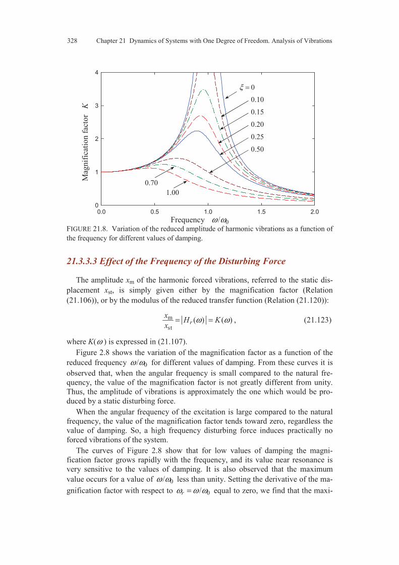
328 Chapter 21 Dynamics of Systems with One Degree of Freedom. Analysis of Vibrations
0.0 0.5 1.0 1.5 2.00
1
2
3
4
Frequency 0/ω ω
Mag
nif
icat
ion
fac
tor
K
0ξ =
0.10
0.15
0.20
0.25
0.50
0.70
1.00
FIGURE 21.8. Variation of the reduced amplitude of harmonic vibrations as a function of
the frequency for different values of damping.
21.3.3.3 Effect of the Frequency of the Disturbing Force
The amplitude xm of the harmonic forced vibrations, referred to the static dis-
placement xst, is simply given either by the magnification factor (Relation
(21.106)), or by the modulus of the reduced transfer function (Relation (21.120)):
m
st
( ) ( )rx
H Kx
ω ω= = , (21.123)
where K(ω ) is expressed in (21.107).
Figure 2.8 shows the variation of the magnification factor as a function of the
reduced frequency 0/ω ω for different values of damping. From these curves it is
observed that, when the angular frequency is small compared to the natural fre-
quency, the value of the magnification factor is not greatly different from unity.
Thus, the amplitude of vibrations is approximately the one which would be pro-
duced by a static disturbing force.
When the angular frequency of the excitation is large compared to the natural
frequency, the value of the magnification factor tends toward zero, regardless the
value of damping. So, a high frequency disturbing force induces practically no
forced vibrations of the system.
The curves of Figure 2.8 show that for low values of damping the magni-
fication factor grows rapidly with the frequency, and its value near resonance is
very sensitive to the values of damping. It is also observed that the maximum
value occurs for a value of 0/ω ω less than unity. Setting the derivative of the ma-
gnification factor with respect to 0/rω ω ω= equal to zero, we find that the maxi-
21.3 Vibrations with Viscous Friction 329
mum occurs for a reduced frequency mrω defined by:
2mm
0
1 2rω
ω ξω
= = − . (21.124)
The maximum amplitude of the amplification factor is then given by:
m m2
1( ) ( )
2 1rK Hω ω
ξ ξ= =
−. (21.125)
For small damping ratios the maximum value of the magnification factor occurs
very near to the undamped natural frequency and the maximum is approximately:
m m1
( ) ( )2
rK Hω ωξ
= ≈ . (21.126)
For example, for 0.20ξ = , the maximum occurs for 00.96 ω and its value is
2.55. Then, when the damping increases, the value of angular frequency mω
decreases and vanishes when 1ξ = .
In the case of low damping, the peak width of the magnification factor can be
evaluated by considering the reduced frequencies rω for which the magnification
factor is reduced by a factor 1/ 2 with respect to the maximum, corresponding to
a reduction of –3 dB. We obtain:
( )2 22 2 2
1 1 1
2 2 11 4r rξ ξω ξ ω
=−− +
. (21.127)
The expansion of this equation leads to:
( )4 2 2 2 42 1 2 1 8 8 0r rω ξ ω ξ ξ− − + − + = . (21.128)
The solutions for this equation are:
( )
( )
2 2 21
2 2 22
2 1 2 2 1 ,
2 1 2 2 1 .
r
r
ω ξ ξ ξ
ω ξ ξ ξ
= − + −
= − − − (21.129)
An approximate solution can be formulated in the case of low values of damping
by expressing that 1rω and 2rω are not greatly different from the frequency mrωof the maximum. Hence:
2 21 2 1 2 1 2 m 1 2( )( ) 2 ( )r r r r r r r r rω ω ω ω ω ω ω ω ω− = + − ≈ − ,
or considering (21.124):
2 2 21 2 2 1 2r r rω ω ξ ∆ω− ≈ − , (21.130)
where r∆ω is the frequency band corresponding to –3 dB reduction centred on

330 Chapter 21 Dynamics of Systems with One Degree of Freedom. Analysis of Vibrations
mrω . Considering Equations (21.129), we finally obtain:
2
2
12
1 2r
ξ∆ω ξ
ξ
−=
−. (21.131)
In the case of low values of the damping, the expression of the bandwidth is
simplified as:
2r∆ω ξ≈ . (21.132)
The frequency response of the damped system is also characterized by the
phase angle ϕ expressed by Equations (21.104) and (21.122). Figure 21.9 shows
the variation of the phase angle as a function of the frequency obtained for
different values of the damping. For frequencies much lower than the natural
frequency of the system, the vibrations are in phase with the imposed force
whatever the value of the damping. Then, the phase angle increases, differently
according to the value of the damping, and reaches a phase delay of /2π (thus a
delay of a quarter-cycle) when the frequency of the force of excitation reaches the
value of the natural frequency. Next, the phase angle continues to increase and
tends towards π for high values of the frequency. This value is reached all the
more quickly than the damping is low.
FIGURE 21.9. Variation of the phase angle as a function of the frequency, for different
values of damping.
0.0 0.5 1.0 1.5 2.0 2.5 3.00
20
40
60
80
100
120
140
160
180
0.1
0ξ =
0.2
0.5
1 2 4
Frequency 0/ω ω
Ph
ase
ang
le
(
°)

21.3 Vibrations with Viscous Friction 331
21.3.4 Forced Vibrations in the case of a Periodic Disturbing Force
In the case where the solid (S) of the spring-mass system of Figure 21.1 is
submitted to a force of horizontal component ( )f t function of time, the motion
equation (21.96) is written:
( )mx cx kx f t+ + = . (21.133)
If the imposed force ( )f t is periodic of period T, the force can be expanded in the
form of Fourier series as:
( )0
1
( ) cos sinn n
n
f t a a n t b n tω ω∞
=
= + + , (21.134)
with 2 /Tω π= . The coefficients a0, an and bn are expressed as:
00
1( ) d
T
a f t tT
= , (21.135)
0
2( )cos d
T
na f t n t tT
ω= , (21.136)
0
2( )sin d
T
nb f t n t tT
ω= . (21.137)
The equation of motion (21.133) is thus written in the reduced form as:
( )20 0 0
1
2 cos sinn n
n
x x x q q n t p n tξω ω ω ω∞
=
+ + = + + , (21.138)
with
00 , , .n n
n na a b
q q pm m m
= = = (21.139)
The general solution of Equation (21.138) consists of the sum of the free vibra-
tions and the forced vibrations. The free vibrations diminish and vanish with
damping. The forced vibrations are obtained by superimposing the steady state
forced vibrations produced by every terms of the second member of Equation
(21.138) These vibrations can be obtained by applying the results obtained in the
previous section (Subsection 21.3.3). In practice, the coefficients of the terms of
the series decrease when n increases. So, the analysis will be limited to a value N
of n for which the terms of upper orders can be neglected. Considering the results
established in Subsection 21.3.3, it can be concluded that forced vibrations with
high amplitudes may occur when the period of one of the terms of series (21.134)
coincides with the period of the natural vibrations of the system, i.e. if the period
T of the disturbing force is equal to, or a multiple of the damped period Td.

332 Chapter 21 Dynamics of Systems with One Degree of Freedom. Analysis of Vibrations
21.3.5 Vibrations in the case of an Arbitrary Disturbing Force
We consider, in this subsection, the case where the spring-mass system is
submitted to an arbitrary force ( )f t . The reduced equation of motion is deduced
from Equation (21.133) and is written:
20 02 ( )x x x q tξω ω+ + = , (21.140)
introducing the force q(t) imposed by unit mass:
1( ) ( )q t f t
m= . (21.141)
The force q(t) is arbitrary. Its variation is represented in Figure 21.10.
At any instant t′ , we may consider (figure 21.10) an impulse of height
( )q t q′ = and width d t′ . This impulse imparts to each unit of mass an instant-
taneous acceleration from the instant t′ given by:
d
dx x q
t= =
′ , (21.142)
which leads to an increase in velocity from t′ given by:
d dx q t′= . (21.143)
regardless of what other forces, such as the spring force, may be acting, and
regardless of the displacement and velocity of solid (S) at the instant t′ . Then, the
increment of displacement at instant t posterior to t′ , is deduced from Equation
(21.75) by substituting the velocity increment (21.143) for the initial velocity 0x
(with a zero initial displacement) and substituting the instant t t′− for instant t (in
Equation (21.75), the disturbing force is exerted at instant 0t = , whereas the
force ( )q t′ is applied at t t′= ). We obtain:
( ) dd sin ( )t t
dd
q tx e t tδ ω
ω′− − ′
′= − . (21.144)
FIGURE 21.10. Arbitrary force as a function of time.
t′ dt′ Time t
Red
uce
d f
orc
e
q(t
)
q

21.3 Vibrations with Viscous Friction 333
Since each impulse ( ) dq t t′ ′ between 0t′ = and t t′ = produces an increment of
displacement given by the preceding expression, the total displacement x(t) which
results from the disturbing force is obtained by integration between 0 and t:
0
( ) ( ) sin ( )dtt
td
d
ex t e q t t t t
δδ ω
ω
−′ ′ ′ ′= − . (21.145)
This form is referred as Duhamel’s integral. It includes both steady state and
transient terms. The integral can be evaluated by an analytical method or a nume-
rical process.
To take account of the effect of possible initial conditions of displacement x0
and velocity 0x , it is necessary to add to the results (21.145) the solution for the
initial conditions considered in Equation (21.75). Thus, the total solution is:
0 00
0 0
1( ) cos sin ( )sin ( )d
tt t
d d dd
x xx t e x t t e q t t t tδ δδ
ω ω ωω ω
′− +′ ′ ′= + + −
.
(21.146)
21.3.6 Forced Vibrations in the case of a Motion Imposed to the Support
21.3.6.1 Equation of Motion
We consider the case where a motion is imposed to the support connected to
one end of the spring (Figure 21.4). The displacement of the solid (S) in the refe-
rence attached to the support is thus expressed by Relation (21.45). The resultant
of the force exerted by the spring is given by Expression (21.46), and the
component of the viscous friction is expressed in (21.55). The motion equation
(21.56) is modified as:
( ) 0smx cx k x x+ + − = , (21.147)
or
smx cx kx kx+ + = . (21.148)
This equation shows that the system is submitted to the imposed force skx .
Equation (21.148) is written in the reduced form:
20 02 sx x x qξω ω+ + = , (21.149)
setting:
20s s s
kq x x
mω= = . (21.150)
Equation (21.149) is identical to the motion equation with an imposed force. We
are brought back to the case studied in Subsections 21.3.3 to 21.3.5.

334 Chapter 21 Dynamics of Systems with One Degree of Freedom. Analysis of Vibrations
y
(T)
(R) (S) G
xxs
FIGURE 21.11. Motion imposed to the support-spring-mass set.
In the case of Figure 21.4, the motion is imposed to the one end of the spring,
the solid (S) remaining in contact with the support. Another case can be consi-
dered (Figure 21.11), where the support-spring-mass set has an imposed motion
with respect to the reference (T). In this case, Expression (21.55) of the
component Xl of friction is modified as:
( )l sX c x x= − , (21.151)
and the equation of motion (21.148) becomes:
s smx cx kx kx cx+ + = + . (21.152)
The system is then submitted to two imposed forces: the one skx and the other
scx . The preceding case is thus a particular case of the present general case.
Equation (21.152) is written in the reduced form:
20 0 1 22 s s sx x x q q qξω ω+ + = = + , (21.153)
with
21 0s s s
kq x x
mω= = , (21.154)
2 10
2s s s
cq x q
m
ξω
= = . (21.155)
21.3.6.2 Case of a Harmonic Motion Imposed to the Support
We consider the case where a harmonic motion is imposed to the support:
m coss sx x tω= . (21.156)
We analyse the most general case of the equation of motion (21.153). The
imposed forces are:
21 0 m coss sq x tω ω= , (21.157)
and
2 m0
2 sins sq x tωξ ωω
= − . (21.158)

21.3 Vibrations with Viscous Friction 335
The total imposed force is:
21 2 m 0
0
cos 2 sins s s sq q q x t tωω ω ξ ωω
= + = −
, (21.159)
which may be put in the form:
( )m coss sq q tω α= − , (21.160)
with
22 2
m m 0 20
1 4s sq xωω ξω
= + , (21.161)
1
0
tan 2ωα ξω
− =
. (21.162)
The equation of motion (21.153) is then written as:
( )20 0 m2 cossx x x q tξω ω ω α+ + = − . (21.163)
It is identical to the motion equation (21.97) obtained in the case of an imposed
force, qm being replaced by msq and the phase angle α being introduced. The
results obtained in Subsection 21.3.3 can then be transposed to the present case.
For the steady state, the response is deduced from Expression (21.102). We obtain:
( )m coss sx x tω α ϕ= − − , (21.164)
with
( ) ( )
2 2 2m 0
m2 22 2
0 0
1 4 /
1 / 2 /
sxx
ξ ω ω
ω ω ξω ω
+=
− +
, (21.165)
1 02 2
0
2 /tan
1 /
ξω ωϕ
ω ω
−=−
. (21.166)
This way of proceeding can also be applied to the case of an arbitrary motion
imposed to the support, while transposing the results derived in Subsection 21.3.5.
21.3.6.3 Case where an Acceleration is Imposed to the Support
We consider the case where a given acceleration sx is imposed at the spring-
mass-support set (Figure 21.11). The equation of motion is given by Equation
(21.152), which is written, introducing the relative displacement xr of the solid
(S), in the form:
r r r smx cx kx mx+ + = − . (21.167)
The second member is equivalent to an imposed force of value smx− . By divi-

336 Chapter 21 Dynamics of Systems with One Degree of Freedom. Analysis of Vibrations
ding Equation (21.167) by the mass m, we obtain the reduced equation of the
motion:
20 02r r r srx x x qξω ω+ + = , (21.168)
with
sr sq x= − . (21.169)
Equation (21.169) is identical to the motion equation with an imposed force. We
are brought back to the cases studied in Sections 21.3.3 to 21.3.5.
21.4 VIBRATIONS WITH DRY FRICTION
21.4.1 Equations of Motion
In the general case, the motion of the solid (S) of Figure (21.1) is characterized
by the first two Equations (21.15):
lmx kx X= − + , (21.170)
lY mg= . (21.171)
In the case of a dry friction between two solids, the components Xl and Yl are
related by the Coulomb’s law (Chapter 13), which introduces the coefficient f of
friction. The Coulomb’s law states that, if the solid (S) is in equilibrium, the
components Xl and Yl are such as:
l lX f Y< ,
Thus, from (21.171):
lX f mg< . (21.172)
If the solid (S) moves, the Coulomb’s law states that components Xl and Yl are
related by the equality:
l lX f Y f mg= = , (21.173)
and that the component Xl is opposed to the velocity of sliding x . The equality
(21.173) can thus be put in the form:
sign( )lX x f mg= − . (21.174)
In the case where the solid is in equilibrium, the equation of motion (21.170)
becomes:
lX kx= . (21.175)
This result associated to the condition (21.172) of friction leads to the relation:
kx f mg< . (21.176)

21.4 Vibrations with Dry Friction 337
Thus, there is equilibrium of the solid if:
2 20 0
1 1fg x fg
ω ω− < < . (21.177)
These inequalities define the limits for the equilibrium of the solid (S).
In the case where the solid (S) moves, Equation (21.170) and the condition
(21.174) of friction leads to the equation of motion:
sign( )mx kx x f mg+ = − , (21.178)
equation which may be rewritten in the reduced form:
20 sign( )x x x f gω+ = − , (21.179)
where 0ω is the natural angular frequency of the spring-mass system without
friction.
Over each interval of time where x keeps a constant sign, the general solution
of the equation of motion is:
1 0 2 0sign( ) cos sinx x f g C t C tω ω= − + + . (21.180)
The values of C1 and C2 depend on the initial conditions for the interval under
consideration. Thus, it results that intervals of time, corresponding to signs of x
which are different, will succeed while satisfying the continuity of the functions
x(t) and ( )x t : the values of the two functions at the end of one interval of time
will provide the initial conditions for the following interval of time.
21.4.2 Free Vibrations
The motion for the free vibrations of the solid (S) is given by Equation
(21.180). So as to illustrate this motion, we consider the case where, at the initial
instant ( 0t = ), the solid is displaced from its equilibrium position by a displace-
ment x0 and the solid is released with a velocity 0x positive.
Following these initial conditions, an episode of motion occurs with 0x > . The
equation of motion is, from (21.180):
1 0 2 0
0 1 0 0 2 0
cos sin ,
sin cos .
x f g C t C t
x C t C t
ω ω
ω ω ω ω
= − + +
= − + (21.181)
The initial conditions impose:
0 1 0 0 2, ,x fg C x Cω= − + =
and the motion (21.181) is written:
( )
( )
00 0 0
0
0 0 0 0 0
cos sin ,
sin cos .
xx fg x fg t t
x x fg t x t
ω ωω
ω ω ω
= − + + +
= − + +
(21.182)

338 Chapter 21 Dynamics of Systems with One Degree of Freedom. Analysis of Vibrations
This episode of motion continues until the instant where x becomes equal to zero,
hence until time t1 such as:
( )1 0
0 10 0
tanx
tx fg
ωω
−=+
. (21.183)
The displacement of the solid reaches thus the value x1:
( ) 01 1 0 0 1 0 1
0
( ) cos sinx
x x t fg x fg t tω ωω
= = − + + +
. (21.184)
At this first episode, an interval of time succeeds with 0x < , of which the
equation of motion starting from the time t1 is:
1 0 1 2 0 1cos ( ) sin ( )x fg C t t C t tω ω= + − + − , (21.185)
with for initial conditions at time t1: 1 1( )x t x= and 1( ) 0x t = . Taking account of
these conditions, the equations of motion are:
( )
( )1 0 1
1 0 0 1
cos ( ),
sin ( ).
x fg x fg t t
x x fg t t
ω
ω ω
= + − −
= − − − (21.186)
This episode of motion continues until the time 2 1 0/2t t T= + 0 0( 2 / ),T π ω= where
the velocity x becomes equal to zero. The displacement of the solid reaches thus
the value x2 given by:
2 1( 2 )x x fg= − − . (21.187)
Two possibilities exist then. Either x2 is included in the limits of equilibrium and
the motion stops. Or x2 is outside these limits, and a new episode of motion occurs
with 0x > .
In the case where the motion continues, the following episode has for equation
of motion, starting from t2:
1 0 2 2 0 2cos ( ) sin ( )x fg C t t C t tω ω= − + − + − , (21.188)
with for initial conditions at time t2: 2 2( )x t x= and 2( ) 0x t = . Hence the equa-
tions of motion:
( )
( )2 0 2
2 0 0 2
cos ( ),
sin ( ).
x fg x fg t t
x x fg t t
ω
ω ω
= − + + −
= − + − (21.189)
This episode continues until time 3 2 0/2t t T= + , where the velocity becomes equal
to zero again. The displacement of the solid reaches then the value x3 given by:
3 2 1( 2 ) 4x x fg x fg= − + = − . (21.190)
At the instant t3, we must consider whether the value of x3 is included or not in
the limits of equilibrium, and so on.
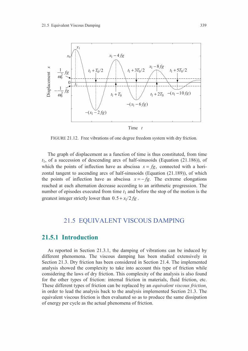
21.5 Equivalent Viscous Damping 339
FIGURE 21.12. Free vibrations of one degree freedom system with dry friction.
The graph of displacement as a function of time is thus constituted, from time
t1, of a succession of descending arcs of half-sinusoids (Equation (21.186)), of
which the points of inflection have as abscissa ,x fg= connected with a hori-
zontal tangent to ascending arcs of half-sinusoids (Equation (21.189)), of which
the points of inflection have as abscissa .x fg= − The extreme elongations
reached at each alternation decrease according to an arithmetic progression. The
number of episodes executed from time t1 and before the stop of the motion is the
greatest integer strictly lower than 10.5 /2x fg+ .
21.5 EQUIVALENT VISCOUS DAMPING
21.5.1 Introduction
As reported in Section 21.3.1, the damping of vibrations can be induced by
different phenomena. The viscous damping has been studied extensively in
Section 21.3. Dry friction has been considered in Section 21.4. The implemented
analysis showed the complexity to take into account this type of friction while
considering the laws of dry friction. This complexity of the analysis is also found
for the other types of friction: internal friction in materials, fluid friction, etc.
These different types of friction can be replaced by an equivalent viscous friction,
in order to lead the analysis back to the analysis implemented Section 21.3. The
equivalent viscous friction is then evaluated so as to produce the same dissipation
of energy per cycle as the actual phenomena of friction.
0-1,5
0,0
1,5
x1
1 4x fg−
1 8x fg−
1( 2 )x fg− −
1( 6 )x fg− −
1( 10 )x fg− −
t1
1 0/2t T+ 1 03 /2t T+ 1 05 /2t T+
1 0t T+ 1 02t T+
x0
0
20
1fg
ω
20
1fg
ω−
Time t
Dis
pla
cem
ent
x

340 Chapter 21 Dynamics of Systems with One Degree of Freedom. Analysis of Vibrations
21.5.2 Energy Dissipated in the case of Viscous Damping
The work done per cycle by the disturbing force m( ) cosf t f tω= during the
steady state response is:
0
cos dT
mW f x t tω= . (21.191)
The velocity x may be obtained by differentiating Expression (21.102) of the dis-
placement with respect to time. Hence:
m sin( )x x tω ω ϕ= − − . (21.192)
Combining Relations (21.191) and (21.192) leads to the expression of the work:
m m sinW x fπ ϕ= . (21.193)
Similarly, the energy aU dissipated per cycle by the viscous damping force cx
is given by:
0
dT
aU cxx t= . (21.194)
Hence, taking account of (21.192), then integrating:
2maU cxπ ω= . (21.195)
For a harmonic steady state, the work done by the disturbing force is equal to the
dissipated energy. From which the amplitude of the displacement is deduced as:
mm sin
fx
cϕ
ω= . (21.196)
When the angular frequency is equal to the natural frequency ( 0ω ω= ), the phase
angle ϕ is /2π and the displacement amplitude is:
mm 0
0
( )f
xc
ωω
= . (21.197)
This result coincides with the result (21.126) obtained for low values of damping.
The equivalent viscous damping constant will be obtained by equating Expres-
sion (21.195) of the energy dissipated by viscous damping to the energy dissi-
pated by the actual damping process. We consider different cases in the following
subsections.
21.5.3 Structural Damping
The structural damping is associated to the internal friction in materials which
are not perfectly elastic. For these materials, the loading stress-strain curve for
increasing levels of stress and strain is different from the unloading curve. Figure
21.13 shows the hysteresis loop obtained in the case of one cycle of vibration.

21.5 Equivalent Viscous Damping 341
FIGURE 21.13. Stress-strain curve for successive loading and unloading of a material.
The experimental results show that the energy dissipated per cycle is approxi-
mately proportional to the square of the strain amplitude. So, the work sU dissi-
pated by structural damping may be written as:
2ms sU xα= , (21.198)
in which sα is a parameter which characterizes the structural damping of the
material considered. Equating Expressions (21.195) and (21.198) of the dissipated
energies leads to the equivalent viscous damping constant:
eqsc
απω
= . (21.199)
The parameter sα has the dimension of a stiffness k and it is usually replaced by
kη , introducing the dimensionless quantity:
s
k
αη
π= . (21.200)
This quantity is called structural damping factor. Relations (21.199) and (21.200),
associated with Relations (21.58) and (21.67) lead to the expression of the
equivalent viscous friction ratio:
eq eq0 0 0
1 1 1
2 2 2
kc
m m
ωξ η ηω ω ω ω
= = = . (21.201)
By substituting this expression into Equation (21.118), the reduced transfer func-
tion is written:
2 20
1( )
1 /rH
iω
ω ω η=
− +, (21.202)
loading
unloading
Strain
Str
ess

342 Chapter 21 Dynamics of Systems with One Degree of Freedom. Analysis of Vibrations
and the magnification factor becomes:
( )
22 2 20
1( ) ( )
1 /
rK Hω ω
ω ω η
= =
− +
. (21.203)
For the natural frequency, the magnification factor is:
0 01
( ) ( )rK Hω ωη
= = , (21.204)
and the amplitude of vibrations is deduced from (21.120):
mm st
1 1 fx x
kη η= = . (21.205)
21.5.4 Dry Friction
In the case of a contact with dry friction between two solids, the process of
friction is generally described by the laws of Coulomb (Relations (21.172) to
(21.174)). These laws introduce the coefficient f of friction. Experiment shows
that, during motion, this coefficient is rather constant, and usually lower than the
coefficient of friction when there is equilibrium.
To determine the equivalent viscous damping, we consider the energy dissi-
pated by the component of friction Xl expressed in (21.173). The energy dissi-
pated fU per cycle is:
f m4 lU f Y x= . (21.206)
In the case of the horizontal spring-mass system (Figure 21.1), we have lY mg= .
In the most general case, lY could be a component of tightening imposed to the
solid (S), orthogonal to the direction of the motion.
By equalling the energy (21.206) to the energy (21.195) dissipated by viscous
friction, we obtain the equivalent friction coefficient:
eqm
4 lf Yc
xπ ω= . (21.207)
In this case, the equivalent friction coefficient depends on the normal component
lY of friction and ω , but also on the amplitude xm of the vibration.
As previously, the equivalent damping ratio eqξ is deduced from Expression
(21.207), associated to Relations (21.58) and (21.67). Thus:
0eq eq
0 m
21
2lf Y
cm x k
ωξ
ω π ω= = . (21.208)
The reduced transfer function (21.118) is written:
21.5 Equivalent Viscous Damping 343
2
2m0
1( )
1 4
rl
Hf Y
ix k
ωω
πω
=
− +
. (21.209)
The amplitude given by Expression (21.120) leads to:
stm
2 22
2m0
41 l
xx
f Y
x k
ωπω
=
− +
. (21.210)
From this expression, we derive the amplitude of the motion:
2
mm st 2
20
41
1
lfY
fx x
π
ω
ω
− = ±
−
. (21.211)
The second term of this expression is the magnification factor. This factor has a
real value if:
m 4lf Y
f
π≤ . (21.212)
In practice where low forces of friction are induced, this condition is satisfied. In
this hypothesis, the magnification factor becomes infinite when the frequency
reaches the value of the natural frequency (Relation (21.211)). This result is
explained by the fact that for the value of the natural frequency, the energy dissi-
pated per cycle is lower than the energy brought by the imposed force. In fact,
Relations (21.206) and (21.212) lead to:
f m mU f xπ< . (21.213)
The expression of the work supplied by the imposed force, shows that, for the
natural frequency 0ω , this work is:
0 m m( )W x fω π= . (21.214)
We verify indeed that for the natural frequency:
f 0( )U W ω< . (21.215)
21.5.5 Fluid Friction
As another type of friction, we consider the case of a solid immersed in a fluid
of low viscosity, such as the air for example. In the case where the mass of the
solid is low and its volume is rather high, it is necessary to take account of the
friction induced by the resistance of the fluid. The force of resistance (Figure
21.14) exerted by the fluid on the solid can be evaluated as:

344 Chapter 21 Dynamics of Systems with One Degree of Freedom. Analysis of Vibrations
FIGURE 21.14. Fluid friction.
2fl t p
1
2R x C Sρ= , (21.216)
where ρ is the mass per unit volume of the fluid, tC the drag coefficient and pS
the area of the section projected in a plane orthogonal to the direction of the
motion. The force of resistance exerted by the fluid is proportional to the square
of the velocity and is opposite to its velocity. The energy Ufl dissipated per cycle
by this force is:
/4
fl fl fl0 0
d 4 dT T
U R x t R x t= = . (21.217)
Introducing Relations (21.102) and (21.216) into the preceding expression, then
integrating, the dissipated energy is written:
3 2fl fl m
8
3U C x ω= , (21.218)
setting:
fl t p1
2C C Sρ= . (21.219)
While identifying the energy (21.218) with the energy dissipated in the case of
viscous damping (21.195), we obtain the equivalent damping coefficient:
eq fl m8
3c C x ω
π= . (21.220)
As previously, the equivalent viscous damping ratio eqξ is deduced from the
preceding expression, considering Relations (21.58) and (21.67):
fl m 0eq
4
3
C x
k
ω ωξ
π= . (21.221)
k
m
(S)
Sp
x

21.5 Equivalent Viscous Damping 345
The reduced transfer function (21.118) is written:
22fl m
20
1( )
1 83
rHC x
ik
ωωω
πω
=
− +
. (21.222)
The amplitude of the vibrations is expressed by (21.120). Thus:
stm
22 22fl m
20
81
3
xx
C x
k
ωωπω
=
− +
. (21.223)
This expression leads to the quadratic equation of which xm is solution:
2 22 24 2 2 2flm m m2
0
81 0
3
Cx k x f
ω ωπ ω
+ − − =
. (21.224)
21.5.6 Conclusion
In conclusion, an equivalent viscous damping may always be considered, what-
ever the dissipative process of energy which is induced. The dissipated energy RU
per cycle is expressed in the form:
0
dT
RU Rx t= , (21.225)
where R is the resultant of the force of resistance to the motion and x is the
velocity of displacement deduced from Expression (21.103).
The equivalent viscous damping coefficient is then evaluated by equalling the
dissipated energy (21.225) with the energy (21.195) induced by the process of
viscous damping. Thus:
eq 2R
m
Uc
xπ ω= . (21.226)
Next, the equivalent viscous damping ratio eqξ is determined by using Relations
(21.58) and (21.67):
eqeq
02
c
mξ
ω= . (21.227)
This viscous damping ratio determines the transfer function ( )rH ω using Relation
(21.118). The modulus of this function relates (21.120) the amplitude of the vibra-
tions to the amplitude of the response obtained in the case of an imposed static
force.
Lastly, let us note that it is also possible to take account simultaneously of
several types of damping.

346 Chapter 21 Dynamics of Systems with One Degree of Freedom. Analysis of Vibrations
( )f t
A
−A
T/4
T/2
3T/4 T 2T
t
EXERCISES
21.1 A wheel rolls (Figure 21.15) over an undulated surface with a constant
speed . The undulated surface can be approximated by a sine curve of equation
sin /y d x lπ= , with d = 30 mm and 1 m.l = A mass m equal to 80 kg is
connected to the axle-tree of the wheel through an elastic device of stiffness k
equal to 150 kN/m. Derive the amplitude of the forced vibrations of the mass, as a
function of the speed of the wheel, considering a viscous damping of the vibra-
tions with a coefficient 0.10.ξ =
21.2 A one degree freedom system is submitted to a periodic force ( )f t of which
the variation as a function of time is reported in Figure 21.16. The function is
characterized by its amplitude A and its period T. Study the vibrations in the case
of the steady state.
FIGURE 21.15. Mass-spring-wheel system.
FIGURE 21.16. Excitation in triangle form.
COMMENTS
The study of the vibrations of a system with one degree of freedom is
particularly important, since the derived results are at the foundation of the
modal analysis of the vibrations of a complex structure. Thus, the reader
interested by the vibratory phenomena will have to pay a great attention to
all the concepts introduced in the present chapter.
x
k
m
Ay

21.5 Equivalent Viscous Damping 347

CHAPTER 22
Motion of Rotation of a Solid about a Fixed Axis
22.1 GENERAL EQUATIONS
22.1.1 Introduction
The motion of rotation about an axis occurs in many industrial applications:
rotors, wheels, crankshafts, revolving machines, etc. The study of the kinematics
of this motion was implemented in Subsection 9.4.1 of Chapter 9. Within the
framework of the present chapter, we consider (Figure 22.1) the motion of rotation
of a solid (S) about a horizontal axis (∆), obtained through a hinge connection
between the solid and the support (T). The solid (S) has a mass m, a mass centre G
and an arbitrary form. The mass centre is distant of a from the axis of rotation.
FIGURE 22.1. Rotation of a solid (S) about the axis (∆).
(S)
G
a
()

348 Chapter 22 Motion of Rotation about a Fixed Axis
xS
(S)
G
a
()
x
yS
y
z
O
FIGURE 22.2. Choice of the coordinate systems.
22.1.2 Parameters of Situation
We choose the coordinate system (Oxyz) attached to the support (T) such as the
axis Oz
coincides with the axis (∆), the axis Ox
has the downward vertical as
direction and such as the mass centre of the solid is contained in the plane (Oxy)
(Figure 22.2).
The parameters of translation are determined while choosing a particular point
of the solid. We choose a point of the axis of rotation: the point O. This point does
not move during the motion of rotation of the solid. Thus, there does not exist any
parameter of translation.
The parameters of rotation are determined while choosing a coordinate system
attached to the solid (S). We choose the system ( )S SOx y z such as the axis SOx
passes through the mass centre G. (Another possible choice could have been to
choose the axis SOx
coinciding with a principal axis of inertia of the solid (S)).
The orientation of the solid (S) is defined by the angle ψ between the axis Ox
and
the axis SOx
.
Finally, the motion is characterized by one parameter of rotation ψ about the
axis Oz
. Between the unit direction vectors ( ), S Si j
of the axes SOx
and SOy
and the unit direction vectors ( ), i j
of the axes Ox
and Oy
, we have from (9.45)
the relation:
cos sin ,
sin cos .
S
S
i i j
j i j
ψ ψ
ψ ψ
= +
= − +
(22.1)

22.1 General Equations 349
22.1.3 Kinematics
22.1.3.1 Kinematic Torsor
The kinematic torsor ( ) TS associated to the motion of rotation of the solid (S)
with respect to the support (T) is defined by its elements of reduction at the point
O: ( ) ( )
( ) ( )
,
( , ) 0.
T TS S
T TO S
R k
O t
ω ψ= =
= =
(22..2)
22.1.3.2 Kinematic Vectors of the Mass Centre
The position of the mass centre is defined by its position vector:
SOG a i=
. (22.3)
The velocity vector of the mass centre can be derived in two ways, either by
using directly the definition of the velocity vector:
( )( )
d( , )d
TT G t OG
t=
, (22.4)
or by using the relation between the velocity vectors of two points of the solid:
( ) ( ) ( ) ( ) ( , ) ( , )T T T T
S SG t O t OG OGω ω= + × = ×
. (22.5)
In the two cases, we obtain: ( )
( , )TSG t a jψ= . (22.6)
This velocity vector can possibly be expressed in the basis ( ), , i j k
of the refe-
rence (T). We obtain: ( )
( , ) sin cosT G t a i a jψ ψ ψ ψ= − + . (22.7)
The acceleration vector of the mass centre is easily obtained by deriving the
velocity vector:
( )( )
( )
d( , ) ( , )d
TT Ta G t G t
t=
. (22.8)
The application of this relation to Expression (22.6) of the velocity vector leads to:
( )
2( , )TS Sa G t a i a jψ ψ= − +
, (22.9)
which expresses the acceleration vector in the basis ( ), , S Si j k
attached to the solid.
The expression of the acceleration in the basis ( ), , i j k
can then be obtained
either by expanding Expression (22.9) considering Relations (22.1) of basis
change, or by deriving directly Expression (22.7). We obtain:
( ) ( ) ( )
2 2( , ) sin cos cos sinTa G t a i a jψ ψ ψ ψ ψ ψ ψ ψ= − + + −
(22.10)

350 Chapter 22 Motion of Rotation about a Fixed Axis
22.1.4 Kinetics
22.1.4.1 Introduction
We have to derive here the elements of reduction of the kinetic and dynamic
torsors. In this way, the question is to know at which point we must determine the
moments of the torsors. In fact, a discerning choice will simplify the resolution of
the equations deduced from the fundamental principle of the dynamics. The
expression of the moment of the dynamic torsor is simpler at the mass centre
(18.9). In a general way, that is this point which will be selected to study the
motion of a solid. However, the fundamental principle of dynamics introduces the
actions of connections, on which it is necessary then to set assumptions on the
physical nature of the induced processes of friction. In this way, the application of
the fundamental principle to the study of the motion of rotation about an axis
shows that the analysis of the problem is made easier while expressing the
moments at a point of the axis of rotation. We choose the point O.
22.1.4.2 Kinetic Torsor
The elements of reduction at the point O of the kinetic torsor ( ) T
S are from
(16.5) and (16.6):
( ) ( ) ( , )T T
S SR m G t ma jψ= =
, (22.11)
( ) ( ) ( ) ( ) ( ) ( ) ( , )T T T T
O S O S O Sm OG O t S Sω ω= × + = . (22.12)
To obtain the moment at the point O, it is necessary to introduce the matrix of in-
ertia( )
( )SbO SI at the point O of the solid (S) expressed in the basis ( ) ( ), , S S Sb i j k=
attached to the solid. Owing to the fact that the axes of the trihedron ( )S SOx y z
are not generally the principal axes of inertia, the matrix of inertia has the general
form:
( )( )Sb
O
A F E
S F B D
E D C
− − = − − − −
I . (22.13)
The expression of the moment is thus:
( )
TO S S SE i D j C kψ ψ ψ= − − +
. (22.14)
22.1.4.3 Dynamic Torsor
The elements of reduction at the point O of the dynamic torsor ( ) T
S are from
(16.15) and (16.16):
( ) ( )( , )T T
SR ma G t= , (22.15)

22.1 General Equations 351
( ) ( ) ( ) ( ) ( ) ( ) ( )
( ) ( ) ( ) ( ) ( )
( , )
.
T T T T TO S O S S O S
T T TO S S O S
m OG a O t S S
S S
ω ω ω
ω ω ω
= × + + ×
= + ×
(22.16)
The resultant of the dynamic torsor is obtained by substituting one of Expres-
sions (22.9) or (22.10) of the acceleration vector into Expression (22.15).
The expression of the moment is written by introducing the matrix of inertia
(22.13). We obtain:
( ) ( ) ( )
2 2TO S S SE D i D E j C kψ ψ ψ ψ ψ= − + − + +
(22.17)
Possibly, the moment can be rewritten in the basis ( ), , i j k
by introducing
Relations (22.1) of basis change into (22.17).
22.1.4.4 Kinetic Energy
The kinetic energy is obtained using the relation:
( ) ( ) ( ) c1( )2
T T TS SE S = ⋅ ,
thus, taking account of (22.2), (22.11) and (22.14):
( ) 2c
1( )2
TE S Cψ= . (22.18)
22.1.5 Mechanical Actions Exerted on the Solid
The mechanical actions exerted on the solid are the action of gravity, the action
of the support induced by the hinge connection and possibly a driving or braking
action.
1. Action of gravity
The action is represented by the torsor ( ) e S of which the elements of
reduction at the mass centre are:
( )
( )
e ,
e 0.G
R S mg i
S
=
=
(22.19)
The power developed by the action of gravity is:
( ) ( ) ( ) ( ) e eT TSP S S= ⋅ . (22.20)
This expression developed at the point O is written:
( ) ( ) ( ) ( ) ( ) ( ) e e ( , ) eT T T
OSP S R S O t Sω= +⋅ ⋅
. (22.21)
It is necessary to express the moment at O of the action of gravity:
( ) ( ) ( ) ( ) e e e eO GS S R S GO OG R S= + × = ×
. (22.22)
352 Chapter 22 Motion of Rotation about a Fixed Axis
Finally, we have:
( ) e sinO S mgak ψ= − . (22.23)
And Expression (22.21) is written:
( ) ( ) e sinTP S mgaψ ψ= − . (22.24)
2. Action of the support induced by the hinge connection
The action of connection exerted by the support is represented by the torsor
( ) S of which the elements of reduction at the point O are:
( )
( )
,
.
l l l
O l S l S l
R S X i Y j Z k
S L i M j N k
= + +
= + +
(22.25)
The components Xl, Yl, ..., Nl, of the action of connection are to be determined.
The power developed by the action of connection is:
( ) ( ) ( ) ( ) T TS lP S S N ψ= =⋅ . (22.26)
3. Driving action or braking action
To put the solid in rotation or to maintain the rotation, it will be necessary to
exert a driving action, which will be reduced to a driving couple. A braking couple
could possibly be applied to stop the rotation. The driving couple or the braking
couple will be represented by a torsor ( )S of which the elements of reduction
at the point O are:
( ) 0,
( ) .O
R S
S N k
=
=
(22.27)
The component N which is imposed is known.
The power developed by this action is:
( ) ( ) ( ) ( )T TSP S S Nψ= =⋅ . (22.28)
22.1.6 Application of the Fundamental Principle of Dynamics
22.1.6.1 General Equations
In the case where the support (T) is attached to the Earth (pseudo-Galilean
reference), the fundamental principle applied to the motion of rotation of the solid
(S) is written:
( ) ( ) ( ) e ( )TS S S S= + + . (22.29)
This equation between torsors leads to the equation of the resultant and to the
equation of the moment at the point O:
22.1 General Equations 353
( ) ( ) ( ) e ( )TSR R S R S R S= + +
, (22.30)
( ) ( ) ( ) e ( )TO O O OS S S S= + +
. (22.31)
The two vector equations of the resultant and of the moment lead then to the six
following scalar equations:
( )( )
( )
2
2
2
2
cos sin ,
sin cos ,
0 ,
,
,
sin .
l
l
l
l
l
l
ma mg X
ma Y
Z
E D L
D E M
C mga N N
ψ ψ ψ ψ
ψ ψ ψ ψ
ψ ψ
ψ ψ
ψ ψ
− + = +
− + =
=
− + =
− + =
= − + +
(22.32)
The theorem of the power-energy:
( )( ) ( ) ( ) ( ) ( ) ( ) cd e ( )d
T T T TE S P S P S P St
= + + (22.33)
leads to the equation:
sin lC mga N Nψψ ψ ψ ψ ψ= − + + . (22.34)
We find the sixth one of Equations (22.32) again.
Finally, we obtain 6 equations for 7 unknowns: Xl, Yl, Zl, Ll, Ml, Nl, ψ. An
additional equation will be derived from the physical nature of the connection.
Thus, the problem is entirely determined.
The consideration of the physical nature of the friction of the hinge connection
will allow us to express the component Nl which is introduced in the expression of
the power developed by the action of connection. Thus the last equation of Equa-
tions (22.32) is the equation of motion, of which the resolution allows us to obtain
the expression of the angle ψ as a function of time. Next, the other components of
the action of connection will be determined by substituting the expression of ψinto the other equations. Note that the moment at O of the action of connection
was expressed in the basis ( ), , S Si j k
attached to the solid. Its expression in the
basis ( ), , i j k
will be then deduced by applying the basis change (22.1). Thus:
( ) ( ) ( )cos sin sin cosO l l l l lS L M i L M j N kψ ψ ψ ψ= − + + +
. (22.35)
22.1.6.2 Rotation with Friction and without Friction
In the case of a perfect connection, i.e. without friction, the power developed
(22.26) is zero. Thus, it results:
0lN = , (22.36)
and the equation of motion is written:
354 Chapter 22 Motion of Rotation about a Fixed Axis
sinC mga Nψ ψ+ = . (22.37)
The expression of ψ as a function of time will depend on the component N of the
driving or braking couple.
In the case of a hinge connection with a friction of viscous type, the component
Nl of connection is opposed to the angular velocity of rotation:
lN cψ= − , (22.38)
and the equation of motion (22.37) is modified as:
sinC c mga Nψ ψ ψ+ + = . (22.39)
22.2 EXAMPLES OF MOTIONS OF ROTATION
ABOUT AN AXIS
22.2.1 Solid in Rotation Submitted only to the Gravity
In the case where the solid (S) is submitted only to the gravity, the solid in
motion of rotation is usually called simple pendulum. Among Equations (22.32),
only the equation of motion is modified and is written:
sin lC mga Nψ ψ= − + . (22.40)
Recall that the parameter C is the moment of inertia of the solid (S), with respect
to the axis of rotation, depending on the geometry and the mass of the solid.
In the case of a connection without friction, the equation of motion is reduced to:
sin 0C mgaψ ψ+ = . (22.41)
The position of equilibrium is obtained when sin 0ψ = ; what leads to the two
values of the angle eq 0ψ = and eqψ π= .
The characterization of the stability of these equilibriums can be evaluated, in
accordance with the following definitions:
The equilibrium of a solid is said to be stable if and only if this solid, slightly
disturbed from its position of equilibrium and then released, swings around this
position and moves back to this position.
The equilibrium of a solid is said to be unstable, if the solid, slightly disturbed
from its position of equilibrium, keeps moving away from this position when the
solid is released.
Thus we search for the motion ε of the solid around the position eqψ of equili-
brium. We have eqψ ψ ε= + , and Equation (22.41) is written:
( )eq eqsin cos cos sin 0C mgaε ψ ε ψ ε+ + = . (22.42)

22.2 Examples of Motions of Rotation about an Axis 355
Expanding to the first order and taking account of the fact that eqsin 0ψ = , we
obtain:
eqcos 0C mgaε ε ψ+ = , (22.43)
or
20 eqcos 0ε ω ε ψ+ = , (22.44)
introducing the natural angular frequency:
20
mga
Cω = . (22.45)
In the case where eq 0ψ = , whence eqcos 1ψ = , Equation (22.44) is written:
20 0ε ω ε+ = . (22.46)
We are brought back to the reduced form (21.24) of the vibrations of a system
with one degree of freedom. The motion of the solid is pendular around the po-
sition of equilibrium eqψ , and the equilibrium is thus stable.
In the case where eqψ π= , whence eqcos 1ψ = − , Equation (22.44) is written:
20 0ε ω ε− = . (22.47)
The motion for low amplitudes is of the form:
0tAeωε = . (22.48)
The function ε is a function which increases with time and the equilibrium is
unstable.
In the case of a connection with viscous friction (22.38), the equation of motion
(22.39) is modified as:
sin 0C c mgaψ ψ ψ+ + = . (22.49)
This equation is written in the form:
202 sin 0ψ δψ ω ψ+ + = , (22.50)
setting:
2
c
Cδ = . (22.51)
Near the position of equilibrium eq 0ψ = , we have sinψ ψ≈ and the equation of
motion (22.50) is reduced to:
202 0ψ δψ ω ψ+ + = (22.52)
We are brought back to the reduced form (21.57) of the vibrations of a system
with one degree of freedom with viscous friction. The results developed in Chap-
ter 21 can thus be applied to the present case.
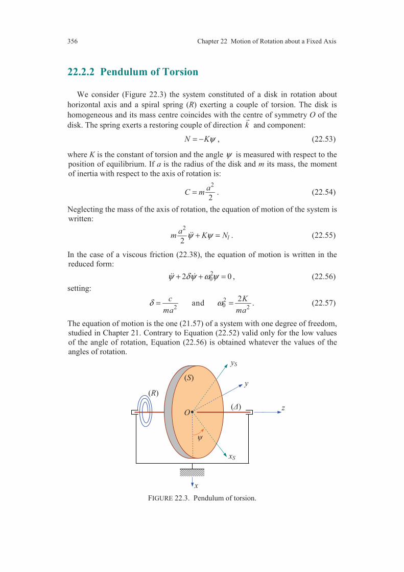
356 Chapter 22 Motion of Rotation about a Fixed Axis
22.2.2 Pendulum of Torsion
We consider (Figure 22.3) the system constituted of a disk in rotation about
horizontal axis and a spiral spring (R) exerting a couple of torsion. The disk is
homogeneous and its mass centre coincides with the centre of symmetry O of the
disk. The spring exerts a restoring couple of direction k
and component:
N Kψ= − , (22.53)
where K is the constant of torsion and the angle ψ is measured with respect to the
position of equilibrium. If a is the radius of the disk and m its mass, the moment
of inertia with respect to the axis of rotation is:
2
2
aC m= . (22.54)
Neglecting the mass of the axis of rotation, the equation of motion of the system is
written: 2
2l
am K Nψ ψ+ = . (22.55)
In the case of a viscous friction (22.38), the equation of motion is written in the
reduced form: 202 0ψ δψ ω ψ+ + = , (22.56)
setting:
202 2
2 and
c K
ma maδ ω= = . (22.57)
The equation of motion is the one (21.57) of a system with one degree of freedom,
studied in Chapter 21. Contrary to Equation (22.52) valid only for the low values
of the angle of rotation, Equation (22.56) is obtained whatever the values of the
angles of rotation.
FIGURE 22.3. Pendulum of torsion.
xS
()
x
yS
y
z
(S)
(R)
O
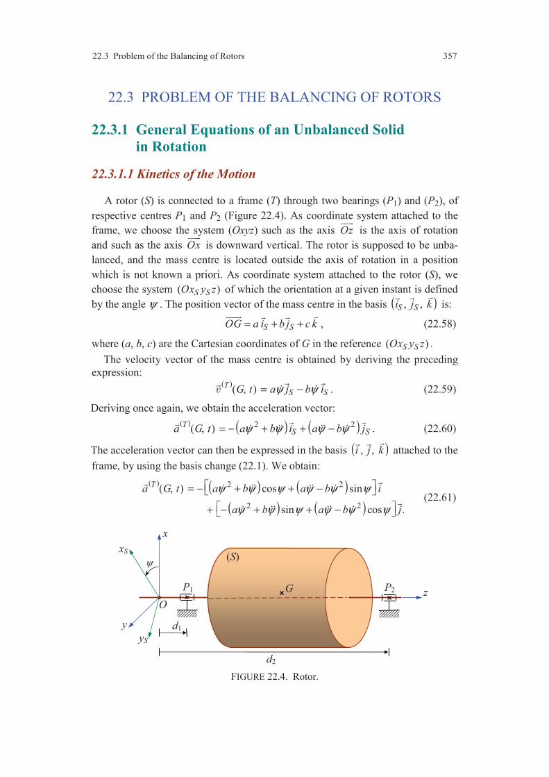
22.3 Problem of the Balancing of Rotors 357
22.3 PROBLEM OF THE BALANCING OF ROTORS
22.3.1 General Equations of an Unbalanced Solid in Rotation
22.3.1.1 Kinetics of the Motion
A rotor (S) is connected to a frame (T) through two bearings (P1) and (P2), of
respective centres P1 and P2 (Figure 22.4). As coordinate system attached to the
frame, we choose the system (Oxyz) such as the axis Oz
is the axis of rotation
and such as the axis Ox
is downward vertical. The rotor is supposed to be unba-
lanced, and the mass centre is located outside the axis of rotation in a position
which is not known a priori. As coordinate system attached to the rotor (S), we
choose the system ( )S SOx y z of which the orientation at a given instant is defined
by the angle ψ . The position vector of the mass centre in the basis ( ), , S Si j k
is:
S SOG a i b j c k= + +
, (22.58)
where (a, b, c) are the Cartesian coordinates of G in the reference ( )S SOx y z .
The velocity vector of the mass centre is obtained by deriving the preceding
expression: ( )
( , )TS SG t a j b iψ ψ= − . (22.59)
Deriving once again, we obtain the acceleration vector:
( ) ( ) ( )
2 2( , )TS Sa G t a b i a b jψ ψ ψ ψ= − + + −
. (22.60)
The acceleration vector can then be expressed in the basis ( ), , i j k
attached to the
frame, by using the basis change (22.1). We obtain:
( ) ( ) ( )
( ) ( )
2 2
2 2
( , ) cos sin
sin cos .
Ta G t a b a b i
a b a b j
ψ ψ ψ ψ ψ ψ
ψ ψ ψ ψ ψ ψ
= − + + −
+ − + + −
(22.61)
FIGURE 22.4. Rotor.
yS
P2G
(S)
O
xS
x
y
z
P1
d1
d2

358 Chapter 22 Motion of Rotation about a Fixed Axis
The resultant of the dynamic torsor is thus:
( ) ( )( , )T T
SR ma G t= , (22.62)
where the acceleration vector of the mass centre is given by the preceding expres-
sion (22.61).
The matrix of inertia at the point O of the rotor (S) expressed in the basis (bS) is
arbitrary and thus expressed in the general form (22.14). The moment at the point
O of the dynamic torsor is then given by Expression (22.17). Expressing this
moment in the basis ( ), , i j k
, we obtain:
( ) ( ) ( )
( ) ( )
2 2
2 2
cos sin
sin cos .
TO S E D D E i
E D D E j C k
ψ ψ ψ ψ ψ ψ
ψ ψ ψ ψ ψ ψ ψ
= − + + +
+ − + − + +
(22.63)
22.3.1.2 Mechanical Actions Exerted on the Rotor
The mechanical actions exerted on the rotor are the action of gravity, the
actions induced by the frame at the level of the bearings and possibly a driving or
braking couple.
1. Action of gravity
The action is represented by the torsor ( ) e S of which the elements of redu-
ction at the mass centre are:
( )
( )
e ,
e 0.G
R S mg i
S
= −
=
(22.64)
The moment at the point O of the action of gravity is:
( ) ( ) e eO S OG R S= ×
, (22.65)
hence:
( ) ( ) e sin cosO S mgcj mg a b kψ ψ= − + + (22.66)
2. Action of the frame exerted at the level of the bearing (P1)
The action is considered to be a force of which the line of action passes through
the centre P1 of the bearing. The action is represented by the torsor ( ) 1 S , of
elements of reduction at the point O:
( )
( )
1
1 1 1 1
1
,
0.P
R S X i Y j Z k
S
= + +
=
(22.67)
The moment at the point O is expressed by:
( ) ( ) 11 1O S OP R S= ×
. (22.68)
Hence:
( ) 1 1 1 1 1O S Y d i X d j= − + (22.69)
where d1 is the distance from the centre of the bearing P1 to the point O (Figure
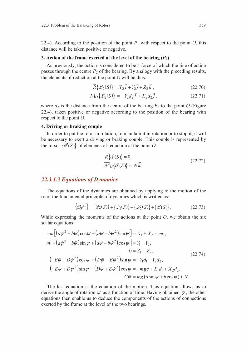
22.3 Problem of the Balancing of Rotors 359
22.4). According to the position of the point P1 with respect to the point O, this
distance will be taken positive or negative.
3. Action of the frame exerted at the level of the bearing (P2)
As previously, the action is considered to be a force of which the line of action
passes through the centre P2 of the bearing. By analogy with the preceding results,
the elements of reduction at the point O will be thus:
( ) 2 2 2 2R S X i Y j Z k= + +
, (22.70)
( ) 2 2 2 2 2O S Y d i X d j= − + , (22.71)
where d2 is the distance from the centre of the bearing P2 to the point O (Figure
22.4), taken positive or negative according to the position of the bearing with
respect to the point O.
4. Driving or braking couple
In order to put the rotor in rotation, to maintain it in rotation or to stop it, it will
be necessary to exert a driving or braking couple. This couple is represented by
the torsor ( )S of elements of reduction at the point O:
( ) 0,
( ) .O
R S
S N k
=
=
(22.72)
22.3.1.3 Equations of Dynamics
The equations of the dynamics are obtained by applying to the motion of the
rotor the fundamental principle of dynamics which is written as:
( ) ( ) ( ) ( ) 1 2e ( )TS S S S S= + + + . (22.73)
While expressing the moments of the actions at the point O, we obtain the six
scalar equations:
( ) ( )
( ) ( )
( ) ( )( ) ( )
2 21 2
2 21 2
1 2
2 21 1 2 2
2 21 1 2 2
cos sin ,
sin cos ,
0 ,
cos sin ,
sin cos ,
sin c
m a b a b X X mg
m a b a b Y Y
Z Z
E D D E Y d Y d
E D D E mgc X d X d
C mg a b
ψ ψ ψ ψ ψ ψ
ψ ψ ψ ψ ψ ψ
ψ ψ ψ ψ ψ ψ
ψ ψ ψ ψ ψ ψ
ψ ψ
− + + − = + −
− + + − = +
= +
− + + + = − −
− + − + = − + +
= +
( )os .Nψ +
(22.74)
The last equation is the equation of the motion. This equation allows us to
derive the angle of rotation ψ as a function of time. Having obtained ψ , the other
equations then enable us to deduce the components of the actions of connections
exerted by the frame at the level of the two bearings.

360 Chapter 22 Motion of Rotation about a Fixed Axis
22.3.2 Mechanical Actions Exerted on the Shaft of Rotor
During the motion of rotation, the mechanical actions exerted on the shaft of
the rotor at the level of the bearings are represented respectively by the torsors
( ) 1 S and ( ) 2 S . Reciprocally, the rotor exerts opposed mechanical actions,
represented by the torsors ( ) 1 S− and ( ) 2 S− . The components (X1, Y1)
and (X2, Y2) are obtained by solving Relations (22.74). We obtain:
( ) ( ) ( )
( ) ( )
( ) ( ) ( )
( ) ( )
2 21 2 2 2 2 2
2 1
2 21 2 2 2 2
2 1
2 22 1 1 1 1 1
2 1
2 22 1 1 1 1
2 1
1sin cos ,
1sin cos ,
1sin cos ,
1sin cos
X mg c d E D D Ed d
Y D E E Dd d
X mg c d E D D Ed d
Y D E E Dd d
ψ ψ ψ ψ ψ ψ
ψ ψ ψ ψ ψ ψ
ψ ψ ψ ψ ψ ψ
ψ ψ ψ ψ ψ
= − − + − + + −
= + + − + −
= − + − + + − −
= − + + −−
,ψ
(22.75)
setting:
1 1 1 1
2 2 2 2
, ,
, .
E E mad D D mbd
E E mad D D mbd
= − = −
= − = − (22.76)
22.3.3 Principle of the Balancing
The components (22.75) of the mechanical actions exerted on the shaft of the
rotor depend on , ψ ψ and more especially on 2ψ . They can thus reach values
rapidly high when ψ increases. Moreover, the shaft is deformable and the rotor-
shaft system behaves in a way similar to that of a system with one degree of
freedom such as that studied in Chapter 21. Vibrations are thus generated which
will lead to a premature deterioration of the shafts or bearings. In order to increase
the life duration of shafts, it is necessary to reduce as well as possible the actions
exerted on the shaft. The examination of Expressions (22.75) shows that the
actions are reduced to minimal values if:
0a b= = , (22.77)
and
0D E= = . (22.78)
The first condition corresponds to the case where the mass centre is located on
the axis of rotation. It is said that the rotor-shaft system is statically balanced. The
equilibrium of the rotor is then indifferent or neutral. The second condition corres-
ponds to the case where the axis of rotation is principal axis of inertia. When these
two conditions are satisfied, it is said that the rotor-shaft system is dynamically
balanced. The components of the actions of connections are then reduced as:
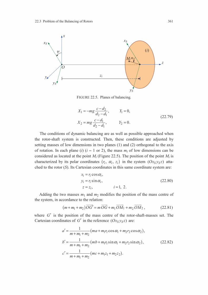
22.3 Problem of the Balancing of Rotors 361
Mi
(i)
O
yS
xS
x
y
z
zi
yS
xS
i
FIGURE 22.5. Planes of balancing.
21 1
2 1
12 2
2 1
, 0,
, 0.
c dX mg Y
d d
c dX mg Y
d d
−= − =
−
−= =
−
(22.79)
The conditions of dynamic balancing are as well as possible approached when
the rotor-shaft system is constructed. Then, these conditions are adjusted by
setting masses of low dimensions in two planes (1) and (2) orthogonal to the axis
of rotation. In each plane (i) (i = 1 or 2), the mass mi of low dimensions can be
considered as located at the point Mi (Figure 22.5). The position of the point Mi is
characterized by its polar coordinates ( ), , i i ir zα in the system ( )S SOx y z atta-
ched to the rotor (S). Its Cartesian coordinates in this same coordinate system are:
cos ,
sin ,
, 1, 2.
i i i
i i i
i
x r
y r
z z i
α
α
=
=
= =
(22.80)
Adding the two masses m1 and m2 modifies the position of the mass centre of
the system, in accordance to the relation:
( ) 1 21 2 1 2m m m OG m OG m OM m OM′+ + = + +
, (22.81)
where G′ is the position of the mass centre of the rotor-shaft-masses set. The
Cartesian coordinates of G′ in the reference ( )S SOx y z are:
( )
( )
( )
1 1 1 2 2 21 2
1 1 1 2 2 21 2
1 1 2 21 2
1cos cos ,
1sin sin ,
1.
a ma m r m rm m m
b mb m r m rm m m
c mc m z m zm m m
α α
α α
′ = + ++ +
′ = + ++ +
′ = + ++ +
(22.82)

362 Chapter 22 Motion of Rotation about a Fixed Axis
Condition (22.77), applied to a′ and b′ , leads to the relations of static balancing:
1 1 1 2 2 2
1 1 1 2 2 2
cos cos 0,
sin sin 0.
ma m r m r
mb m r m r
α α
α α
+ + =
+ + = (22.83)
The matrix of inertia at the point O of the mass mi considered as located at the
point Mi is:
( )
( )( )
( )
2 2
2 2
2 2
( )S
i i i i i i i i i
bi i i i i i i i i iO
i i i i i i i i i
m y z m x y m x z
M m x y m x z m y z
m x z m y z m x y
+ − − = − + −
− − +
I . (22.84)
The matrix of inertia at the point O of the rotor-shaft-masses set is written as:
( ) ( ) ( )1 2( ) ( ) ( )S S Sb b b
O O OS M M+ +I I I . (22.85)
In particular, the moments of inertia D and E of the rotor are modified respect-
tively according to the expressions:
1 1 1 1 2 2 2 2
1 1 1 1 2 2 2 2
sin sin ,
cos cos .
D D m r z m r z
E E m r z m r z
α α
α α
′ = + +
′ = + + (22.86)
The conditions (22.78) applied to D′ and E′ lead to the relations:
1 1 1 1 2 2 2 2
1 1 1 1 2 2 2 2
sin sin 0,
cos cos 0.
D m r z m r z
E m r z m r z
α α
α α
+ + =
+ + = (22.87)
Relations (22.83) and (22.87) constitute the four relations of dynamic balancing of
a rotor.
Usually the masses are set in given planes, easily accessible. The relations of
balancing thus allow us to derive four of the parameters ( ) 1 1 1, ,m r α and
( ) 2 2 2, , ,m r α in fact two of the parameters ( ) 1 1 1, ,m r α and two of the parameters
( ) 2 2 2, , .m r α The choice of the parameters will be conditioned to facilities of
implementation. In practice, balancing is carried out by using an electronic system
of balancing. The mechanical actions exerted on the axis of rotation are measured
using accelerometers. Preliminary measurements make it possible to determine
the parameters a, b, D and E of the unbalanced rotor, and then to deduce the four
parameters of balancing by Relations (22.83) and (22.87).
EXERCISES
22.1 Analyse the motion of a parallelepiped connected to a support by a hinge
connection of horizontal axis passing through its mass centre and submitted to the
action of a spiral spring (R) exerting a couple of torsion (Figure 22.6).
22.2 Analyse the motion of a parallelepiped in the case of a hinge connection of
eccentric horizontal axis (Figure 22.7a).

Exercises 363
FIGURE 22.6. Motion of a parallelepiped around an axis passing through its centre.
22.3 Analyse the motion of a parallelepiped connected with a hinge connection
of eccentric horizontal axis and submitted to the action of a spiral spring (R)
exerting a couple of torsion (Figure 22.7b).
FIGURE 22.7. Motion of a parallelepiped around an eccentric axis: a) without spring of
torsion and b) with a spring of torsion.
G
(R)
G
Od
(R)
G
Od

364 Chapter 22 Motion of Rotation about a Fixed Axis
COMMENTS
The motion of rotation about an axis occurs in many industrial appli-
cations, such as rotors, wheels, crankshafts, revolving machines, etc. The
motion of rotation induces actions exerted at the level of the connections
which can lead to a deterioration of the connections and shafts. This
problem is solved by implementing a balancing of the rotor and will be
considered by the reader with a great attention.

CHAPTER 23
Plane Motion of a Rigid Body
23.1 INTRODUCTION
Kinematics of a plane motion of a rigid body was studied in Subsection 9.4.5.
The motion of a solid relatively to a given reference is a plane motion, if an only
if a plane attached to the solid remains in coincidence, during the motion, with a
plane attached to the reference. In the most general case, the motion is then defi-
ned by two parameters of translation and one parameter of rotation. In this chapter,
we analyse three examples of plane motion: the motion of a parallelepiped moving
on an inclined plane, the sliding and rocking of a parallelepiped on an inclined
plane, the rolling and sliding of a cylinder on an inclined plane.
23.2 PARALLELEPIPED MOVING
ON AN INCLINED PLANE
23.2.1 Parameters of Situation and Kinematics
We consider (Figure 23.1) the motion of the parallelepiped (S) on the inclined
plane (T), of inclination α with respect to a horizontal plane. During the motion,
the plane (ABCD) of the parallelepiped remains in coincidence with the plane (T).
As coordinate system attached to the plane (T), we choose the trihedron (Oxyz) of
which the plane (Oxy) coincides with the plane (T) and such as the axis Ox
is the
direction of greater slope. As coordinate system attached to the solid (S), we
choose the trihedron ( )S SAx y z constructed on the edges of the parallelepiped.
During the motion, the z-coordinate of the mass centre is constant. The situation
of the solid (S) is then determined by:
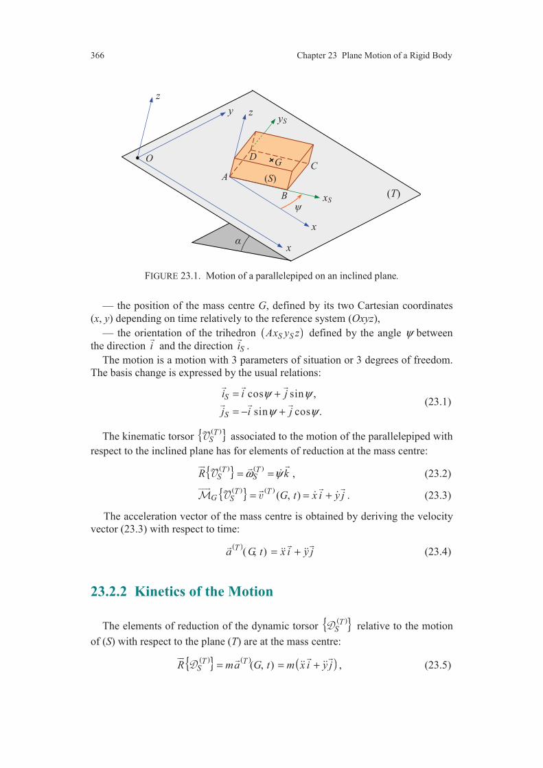
366 Chapter 23 Plane Motion of a Rigid Body
FIGURE 23.1. Motion of a parallelepiped on an inclined plane.
— the position of the mass centre G, defined by its two Cartesian coordinates
(x, y) depending on time relatively to the reference system (Oxyz),
— the orientation of the trihedron ( )S SAx y z defined by the angle ψ between
the direction i
and the direction Si
.
The motion is a motion with 3 parameters of situation or 3 degrees of freedom.
The basis change is expressed by the usual relations:
cos sin ,
sin cos .
S
S
i i j
j i j
ψ ψ
ψ ψ
= +
= − +
(23.1)
The kinematic torsor ( ) TS associated to the motion of the parallelepiped with
respect to the inclined plane has for elements of reduction at the mass centre:
( ) ( )T TS SR kω ψ= =
, (23.2)
( ) ( ) ( , )T T
G S G t x i y j= = +
. (23.3)
The acceleration vector of the mass centre is obtained by deriving the velocity
vector (23.3) with respect to time:
( ) ( , )Ta G t x i y j= + (23.4)
23.2.2 Kinetics of the Motion
The elements of reduction of the dynamic torsor ( ) T
S relative to the motion
of (S) with respect to the plane (T) are at the mass centre:
( ) ( ) ( ) ( , )T TSR ma G t m x i y j= = +
, (23.5)
z
G
A
B
CD
(S)
x
x
xS
yS
y z
(T)
O

23.2 Parallelepiped Moving on an Inclined Plane 367
( ) ( ) ( ) ( ) ( ) ( )T T T TG S G S S G SS Sω ω ω= + ×
. (23.6)
The operator of inertia at the point G is represented in the basis ( ) ( ), , S S Sb i j k=
by the matrix of inertia:
( )0 0
( ) 0 0
0 0
SbG
A
S B
C
=
I , (23.7)
with:
( ) ( ) ( )2 2 2 2 2 2, , ,12 12 12
m m mA b c B a c C a b= + = + = + (23.8)
where m is the mass of the solid and (a, b, c) the respective lengths of the edges of
the parallelepiped. The moment at the mass centre of the dynamic torsor is thus:
( ) ( )
2 2
12T
G Sm
C k a b kψ ψ= = + (23.9)
The kinetic energy can be determined from Relation (16.27). We obtain:
( ) ( ) ( )2 2 2 2 2c
1( )2 24
T mE S m x y a b ψ= + + + . (23.10)
The first term is the kinetic energy of translation, and the second term is the
kinetic energy of rotation.
23.2.3 Mechanical Actions Exerted on the Parallelepiped
The mechanical actions exerted on the parallelepiped are reduced to the action
of gravity and the action of contact exerted by the inclined plane.
1. Action of gravity
The action is represented by the torsor ( ) e S of which the elements of
reduction at the mass centre are:
( )
( )
e ,
e 0,G
R S mg u
S
=
=
(23.11)
where u
is the unit vector of the downward vertical direction:
sin cosu i kα α= −
.
Hence:
( ) ( )e sin cosR S mg i kα α= −
. (23.12)
The power developed by the action of gravity is:
( ) ( ) ( ) ( ) e e sinT TSP S S mgx α= =⋅ . (23.13)
368 Chapter 23 Plane Motion of a Rigid Body
2. Action of contact exerted by the inclined plane
The action of contact is represented by the torsor ( ) S , of which the ele-
ments of reduction at the mass centre are:
( )
( )
,
.
l l l
G l l l
R S X i Y j Z k
S L i M j N k
= + +
= + +
(23.14)
The components Xl, Yl, ..., Nl, of the action of contact are to be determined.
The power developed by the action of contact is:
( ) ( ) ( ) ( ) T TS l l lP S S X x Y y N ψ= = + +⋅ . (23.15)
23.2.4 Equations Deduced from the Fundamental Principle
In the case where the inclined plane is a pseudo-Galilean reference (attached to
the Earth), the fundamental principle applied to the motion of the parallelepiped is
written: ( ) ( ) ( ) eT
S S S= + . (23.16)
The equation of the resultant and that of the moment at the mass centre lead to the
six scalar equations:
sin ,
,
0 cos ,
0 ,
0 ,
.
l
l
l
l
l
l
mx mg X
my Y
mg Z
L
M
C N
α
α
ψ
= +
=
= − +
=
=
=
(23.17)
The theorem of power-energy:
( )( ) ( ) ( ) ( ) ( ) cd ed
T T TE S P S P St
= + (23.18)
leads to the equation:
( ) ( ) ( )2 2 sin12
l l lm
m xx yy a b mg X x Y y Nψψ α ψ+ + + = + + + . (23.19)
This equation is a linear combination of Equations (23.17). In the present case, the
theorem of power-energy does not lead to an equation being of an interest.
Finally, we obtain 6 equations for 9 unknowns: Xl, Yl, Zl, Ll, Ml, Nl, x, y, ψ.
Three equations are solved:
cos ,
0, 0.
l
l l
Z mg
L M
α=
= = (23.20)
23.2 Parallelepiped Moving on an Inclined Plane 369
The three others are the equations of motion:
sin ,
,
.
l
l
l
mx mg X
my Y
C N
α
ψ
= +
=
=
(23.21)
The physical nature of the action of contact allows us to express the components
Xl, Yl, Nl and to deduce from (23.21) the expressions of x, y and ψ as functions of
time.
23.2.5 Motion without Friction
In the case where the contact is perfect between the plane and the solid
(absence of friction), the power developed (23.15) by the action of contact is zero:
0l l lX x Y y N ψ+ + = . (23.22)
This relation is satisfied, whatever , and x y ψ , if:
0, 0, 0.l l lX Y N= = = (23.23)
Equations (23.21) of the motion are then written:
sin ,
0,
0.
x g
y
α
ψ
=
=
=
(23.24)
The integration of these equations gives first:
0
0
0
sin ,
,
.
x gt x
y y
α
ψ ψ
= +
=
=
(23.25)
Then
20 0
0 0
0 0
1sin ,
2
,
,
x gt x t x
y y t y
t
α
ψ ψ ψ
= + +
= +
= +
(23.26)
where 0 0 0 0 0 0, , , , and x y x yψ ψ are the respective values of , , , , and x y x yψ ψ
at the initial time 0t = .
The trajectory of the mass centre G is a parabola contained in the plane parallel
to the inclined plane and distant of c/2. The parabola is tangent to the axis
( )0 0,G , G0 being the position of the mass centre at 0t = :
0 0 02
cOG x i y j k= + +
, (23.27)
370 Chapter 23 Plane Motion of a Rigid Body
and 0
being the velocity vector of G at 0t = :
0 0 0 .x i y j= +
(23.28)
The motion of the mass centre G is accelerated along the axis Ox
and uniform
along the axis Oy
. Once initiated, the motion does not stop. To this motion, a
motion of rotation of the parallelepiped is superimposed about the axis ( ),G k
.
23.2.6 Motion with Dry Friction
In the case where there is dry friction, we make the assumption that the plane
exerts a force of resistance to sliding of resultant tR
and a couple of resistance to
spinning of moment n
, satisfying the laws (13.2) to (13.25) of dry friction. The
resultant and the moment are expressed by:
t l lR X i Y j= +
(23.29)
and
n lN k=
(23.30)
Moreover, the normal force of contact is expressed by:
cosn lR Z k fmg kα= =
, (23.31)
where f is the coefficient of dry friction between the parallelepiped and the plane.
In the case where there is motion, the magnitude of the force of resistance to
sliding is expressed from (13.6) by:
2 2 cosl lX Y fmg α+ = , (23.32)
and the resultant is opposed to the velocity vector of the mass centre. Hence:
( ) ( ) ( , ) 0, with ( , ) 0.T T
t tR G t R G t× = <⋅
Thus
0, with 0.l l l lX y Y x X x Y y− = + < (23.33)
Substituting the first two equations of Equations (23.21) of motion into Expres-
sions (23.30) and (23.31), we obtain the equations of the motion of the mass
centre:
( )
( )
2 2 2 2 2sin cos ,
sin 0,
0.
x g y f g
x g y yx
yy
α α
α
− + =
− − =
<
(23.34)
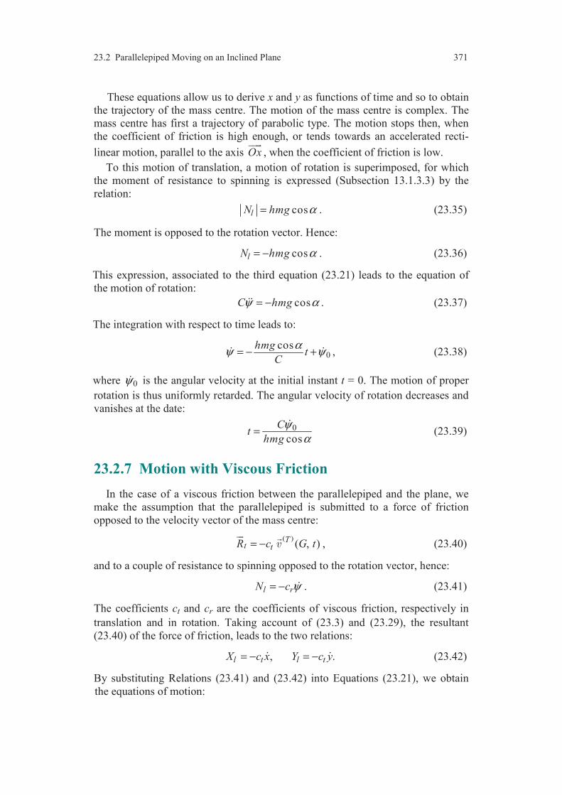
23.2 Parallelepiped Moving on an Inclined Plane 371
These equations allow us to derive x and y as functions of time and so to obtain
the trajectory of the mass centre. The motion of the mass centre is complex. The
mass centre has first a trajectory of parabolic type. The motion stops then, when
the coefficient of friction is high enough, or tends towards an accelerated recti-
linear motion, parallel to the axis Ox
, when the coefficient of friction is low.
To this motion of translation, a motion of rotation is superimposed, for which
the moment of resistance to spinning is expressed (Subsection 13.1.3.3) by the
relation:
coslN hmg α= . (23.35)
The moment is opposed to the rotation vector. Hence:
coslN hmg α= − . (23.36)
This expression, associated to the third equation (23.21) leads to the equation of
the motion of rotation:
cosC hmgψ α= − . (23.37)
The integration with respect to time leads to:
0coshmg
tC
αψ ψ= − + , (23.38)
where 0ψ is the angular velocity at the initial instant t = 0. The motion of proper
rotation is thus uniformly retarded. The angular velocity of rotation decreases and
vanishes at the date:
0
cos
Ct
hmg
ψα
=
(23.39)
23.2.7 Motion with Viscous Friction
In the case of a viscous friction between the parallelepiped and the plane, we
make the assumption that the parallelepiped is submitted to a force of friction
opposed to the velocity vector of the mass centre:
( ) ( , )T
t tR c G t= −
, (23.40)
and to a couple of resistance to spinning opposed to the rotation vector, hence:
l rN c ψ= − . (23.41)
The coefficients ct and cr are the coefficients of viscous friction, respectively in
translation and in rotation. Taking account of (23.3) and (23.29), the resultant
(23.40) of the force of friction, leads to the two relations:
, .l t l tX c x Y c y= − = − (23.42)
By substituting Relations (23.41) and (23.42) into Equations (23.21), we obtain
the equations of motion:
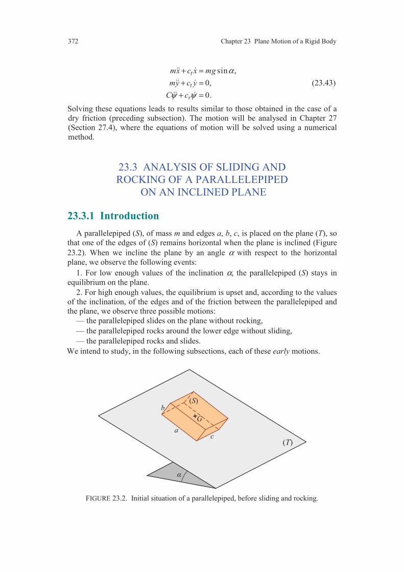
372 Chapter 23 Plane Motion of a Rigid Body
sin ,
0,
0.
t
t
r
mx c x mg
my c y
C c
α
ψ ψ
+ =
+ =
+ =
(23.43)
Solving these equations leads to results similar to those obtained in the case of a
dry friction (preceding subsection). The motion will be analysed in Chapter 27
(Section 27.4), where the equations of motion will be solved using a numerical
method.
23.3 ANALYSIS OF SLIDING AND
ROCKING OF A PARALLELEPIPED
ON AN INCLINED PLANE
23.3.1 Introduction
A parallelepiped (S), of mass m and edges a, b, c, is placed on the plane (T), so
that one of the edges of (S) remains horizontal when the plane is inclined (Figure
23.2). When we incline the plane by an angle α with respect to the horizontal
plane, we observe the following events:
1. For low enough values of the inclination α, the parallelepiped (S) stays in
equilibrium on the plane.
2. For high enough values, the equilibrium is upset and, according to the values
of the inclination, of the edges and of the friction between the parallelepiped and
the plane, we observe three possible motions:
— the parallelepiped slides on the plane without rocking,
— the parallelepiped rocks around the lower edge without sliding,
— the parallelepiped rocks and slides.
We intend to study, in the following subsections, each of these early motions.
FIGURE 23.2. Initial situation of a parallelepiped, before sliding and rocking.
G
(S)
(T)
ac
b
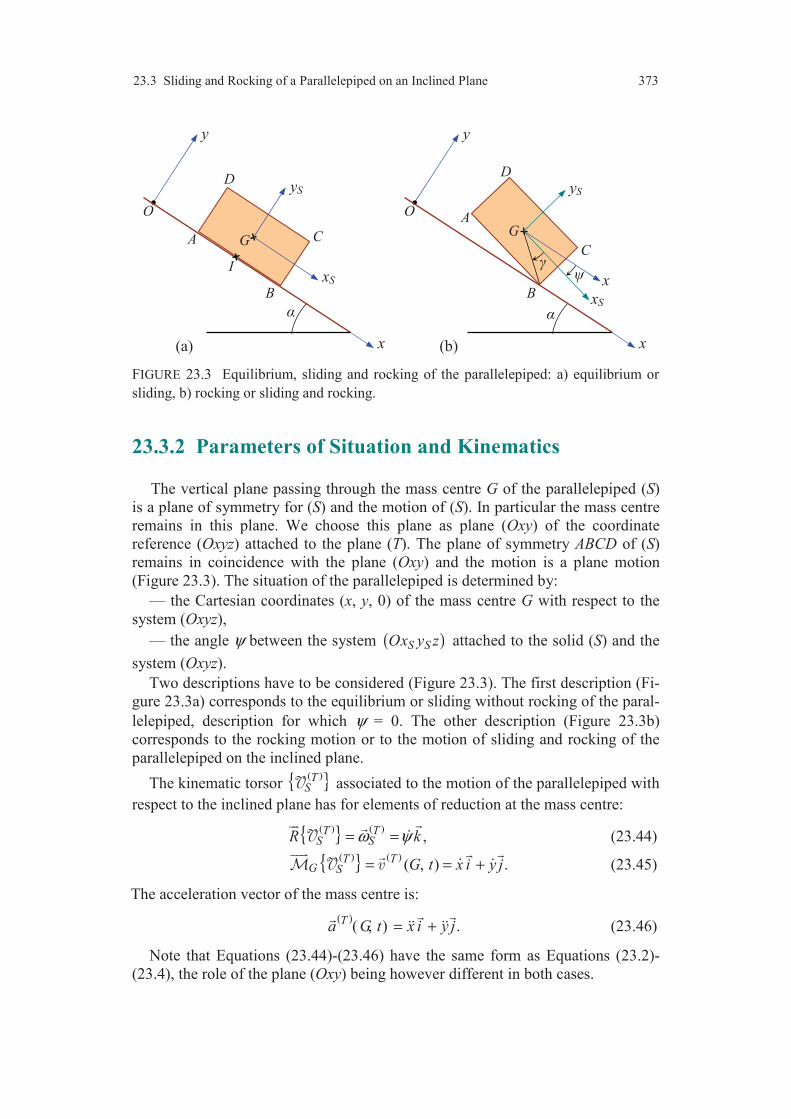
23.3 Sliding and Rocking of a Parallelepiped on an Inclined Plane 373
FIGURE 23.3 Equilibrium, sliding and rocking of the parallelepiped: a) equilibrium or
sliding, b) rocking or sliding and rocking.
23.3.2 Parameters of Situation and Kinematics
The vertical plane passing through the mass centre G of the parallelepiped (S)
is a plane of symmetry for (S) and the motion of (S). In particular the mass centre
remains in this plane. We choose this plane as plane (Oxy) of the coordinate
reference (Oxyz) attached to the plane (T). The plane of symmetry ABCD of (S)
remains in coincidence with the plane (Oxy) and the motion is a plane motion
(Figure 23.3). The situation of the parallelepiped is determined by:
— the Cartesian coordinates (x, y, 0) of the mass centre G with respect to the
system (Oxyz),
— the angle ψ between the system ( )S SOx y z attached to the solid (S) and the
system (Oxyz).
Two descriptions have to be considered (Figure 23.3). The first description (Fi-
gure 23.3a) corresponds to the equilibrium or sliding without rocking of the paral-
lelepiped, description for which ψ = 0. The other description (Figure 23.3b)
corresponds to the rocking motion or to the motion of sliding and rocking of the
parallelepiped on the inclined plane.
The kinematic torsor ( ) TS associated to the motion of the parallelepiped with
respect to the inclined plane has for elements of reduction at the mass centre:
( ) ( ),T T
S SR kω ψ= = (23.44)
( ) ( ) ( , ) .T T
G S G t x i y j= = +
(23.45)
The acceleration vector of the mass centre is:
( ) ( , ) .Ta G t x i y j= + (23.46)
Note that Equations (23.44)-(23.46) have the same form as Equations (23.2)-
(23.4), the role of the plane (Oxy) being however different in both cases.
A
B
C
D
x
xS
yS
y
O
G
x
GA
B
C
D
x
xS
yS
y
O
I
(a) (b)

374 Chapter 23 Plane Motion of a Rigid Body
23.3.3 General Equations
The mechanical actions exerted on the parallelepiped are reduced to the action
of gravity and the action of contact exerted by the inclined plane. The action of
gravity is represented by the torsor ( ) e S of which the elements of reduction at
the mass centre are:
( ) ( )
( )
e sin cos ,
e 0.G
R S mg i k
S
α α= −
=
(23.47)
The action of contact exerted by the plane is represented by the torsor ( ) S of
elements of reduction at G:
( )
( )
,
.
l l l
G l l l
R S X i Y j Z k
S L i M j N k
= + +
= + +
(23.48)
The fundamental principle of dynamics expressed in the reference (T), consi-
dered as pseudo-Galilean reference is written as:
( ) ( ) ( ) eTS S S= + . (23.49)
The dynamic torsor associated to the motion of the solid (S) with respect to the
reference (T) has elements of reduction at the mass centre whose expressions are
identical to those found in (23.5) and (23.9). The fundamental principle leads thus
to the six scalar equations:
sin ,
cos ,
0 ,
0 ,
0 ,
.
l
l
l
l
l
l
mx mg X
my mg Y
Z
L
M
C N
α
α
ψ
= +
= − +
=
=
=
=
(23.50)
We have 6 equations to determine 9 unknowns. So as to supplement these
equations, we admit that the parallelepiped-plane contact is a dry friction contact
characterized by the coefficient of friction f and the action exerted by the plane on
the parallelepiped is a force of which the support passes through a point I of the
surface of contact. This point is located between A and B in the case where there is
equilibrium or sliding (Figure 23.3a), or coincides with the point B in the case
where there is rocking (Figure 23.3b). The validity of this description is verified
by the good agreement which is observed between the experimental facts and the
results that we will deduce from this modelling. We have thus an additional vector
equation:
( ) ( ) ( ) 0I GS S R S GI= + × =
. (23.51)

23.3 Sliding and Rocking of a Parallelepiped on an Inclined Plane 375
This equation leads to:
( ) ( ) G l lS X i Y j IG= + × . (23.52)
Furthermore, the laws of friction allow us to write:
0lY > , (23.53)
l lX f Y= − , (23.54)
if the solid slides on the plane, and:
l lX f Y< , (23.55)
if the solid does not slide.
23.3.4 Analysis of the Different Motions
23.3.4.1 Equilibrium of theParallelepiped
When the parallelepiped is in equilibrium, we have 0x y ψ= = = , and Equa-
tions (23.50) are written:
( )
sin 0,
cos 0,
0,
0.
l
l
l
G
X mg
Y mg
Z
S
α
α
+ =
− =
=
=
(23.56)
The components of the resultant of the action of contact exerted by the plane on
the parallelepiped are thus:
sin , cos , 0.l l lX mg Y mg Zα α= − = = (23.57)
Moreover the forth equation (23.56) associated to Relation (23.52) leads to:
( ) 0l lX i Y j IG+ × =
, (23.58)
or
( ) 02 2
l lb a
X AI Y+ − = , (23.59)
writing:
( )2 2
a bIG AI i j= − − +
. (23.60)
The position of the point I is thus given by:
( )1tan
2AI a b α= + . (23.61)
The condition (23.55) of non sliding and the condition that the point I is between
the points A and B (0 )AI a< < lead to the inequalities:
tan and tan .a
fb
α α< < (23.62)

376 Chapter 23 Plane Motion of a Rigid Body
23.3.4.2 Sliding without Rocking of the Parallelepiped
Sliding without rocking of the parallelepiped occurs when 0y ψ= = , with
0x > . Equations (23.50) are written
( )
sin ,
0 cos ,
0 ,
0.
l
l
l
G
mx mg X
mg Y
Z
S
α
α
= +
= − +
=
=
(23.63)
As previously, the last relation leads to Expression (23.61) of the position of the
point I. Equations (23.63) are associated to the conditions:
0,
0, ,
0 .
l l l
x
Y X fY
AI a
>
> = −
< <
(23.64)
Combining (23.63) and (23.64) leads to:
( )
cos ,
cos
sin cos ,
l
l
Y mg
X fmg
x g f
α
α
α α
=
= −
= −
(23.65)
with the conditions:
tan , .a
f fb
α > < (23.66)
The equation of motion is given by the last equation (23.65). The motion is
uniformly accelerated of equation:
( ) 20 0
1sin cos
2x g f t x t xα α= − + + , (23.67)
where 0x et 0x are the respective values of x and x at the initial instant 0t = .
23.3.4.3 Rocking without Sliding of the Parallelepiped
In the case of a motion with rocking of the parallelepiped (Figure 23.3.b), the
position of the mass centre G is related to that of the point B of contact by the
relation:
( )OG OB GB OB l u ψ γ= − = − +
, (23.68)
with
2 2 11 and tan
2
bl a b
aγ −= + = , (23.69)
and where ( )u ψ γ+
is the unit vector of the direction forming an angle of ψ γ+
with the direction i
. The coordinates of the mass centre are thus expressed as
follows:

23.3 Sliding and Rocking of a Parallelepiped on an Inclined Plane 377
( ) cos( ),
sin( ),
x x B l
y l
ψ γ
ψ γ
= − +
= − + (23.70)
where x(B) is the abscissa of the point B on the axis Ox
.
In the case where there is not sliding of the point B, the abscissa x(B) is inde-
pendent of time and we obtain by deriving (23.70) with respect to time:
sin( ),
cos( ),
x l
y l
ψ ψ γ
ψ ψ γ
= +
= − +
(23.71)
and then:
2
2
sin( ) cos( ) ,
cos( ) sin( ) .
x l
y l
ψ ψ γ ψ ψ γ
ψ ψ γ ψ ψ γ
= + + +
= − + − +
(23.72)
We examine the case of the early motion, for which 0ψ ≈ and 0ψ ≈ . Equations
(23.72) are then written:
sin ,
cos ,
x l
y l
ψ γ
ψ γ
=
= −
(23.73)
and Equations (23.50) become:
( )
sin sin ,
cos cos ,
0 ,
.
l
l
l
G
ml mg X
ml mg Y
Z
S C k
ψ γ α
ψ γ α
ψ
= +
− = − +
=
=
(23.74)
The last equation may be rewritten taking account of the fact that the action of
contact exerted by the plane is, for this motion, a force of which the line of action
passes through the point B. Thus:
( ) ( ) ( ) 0B G l lS S X i Y j GB= + + × = , (23.75)
with
( )GB l u ψ γ= +
. (23.76)
Hence finally the characteristic equations of the motion:
sin sin ,
cos cos ,
0,
sin cos ,
l
l
l
l l
ml X mg
ml Y mg
Z
C X Y
ψ γ α
ψ γ α
ψ γ γ
= +
− = −
=
= − +
(23.77)
equations for which it is necessary to add the conditions:
0, 0, .l l lY X f Yψ < < < (23.78)

378 Chapter 23 Plane Motion of a Rigid Body
Solving Equations (23.77), with respect to the unknowns ψ, Xl and Yl leads to:
( )( )
2 2
2
2
3cos( ),
2
3 31 sin sin sin cos cos ,
4 4
3 31 sin cos sin cos sin .
4 4
l
l
g
a b
X mg
Y mg
ψ α γ
γ α γ γ α
γ α γ γ α
= −+
= − − −
= − −
(23.79)
The motion of rotation about the point D is uniformly accelerated. The angle γbeing negative, the second condition (23.78) is always satisfied. The condition
0ψ < leads to:
1tan
tanα
γ> − , (23.80)
and the condition l lX f Y< is written:
( ) ( )2 23 3 3 31 sin sin cos tan 1 sin sin cos
4 4 4 4f fγ γ γ α γ γ γ − + < − +
. (23.81)
23.3.4.4 Rocking and Sliding of the Parallelepiped
In the case of the motion of rocking and sliding of the parallelepiped, the
coordinates of the mass centre are given by Relations (23.70). In the present
motion, the abscissa of the point B depends on time and the component x of the
acceleration vector is written:
2( ) sin( ) cos( )x x B l ψ ψ γ ψ ψ γ = + + + + , (23.82)
and for the early motion:
( ) sinx x B lψ γ= + . (23.83)
The equations of the early motion are thus from (23.50):
[ ]( ) sin sin ,
cos cos ,
0,
sin cos ,
l
l
l
l l
m x B l X mg
ml Y mg
Z
C X Y
ψ γ α
ψ γ α
ψ γ γ
+ = +
− = −
=
= − +
(23.84)
equations to which it is necessary to associate the conditions:
( ) 0, 0, 0, l l lx B Y X f Yψ> < > = − . (23.85)
Solving Equations (23.84) leads to:
( )22 2
6 cos sin cos1,
1 3 sin cos 3cos
fg
fa b
γ γ αψ
γ γ γ
+=
+ ++

23.3 Sliding and Rocking of a Parallelepiped on an Inclined Plane 379
( )2
2
3sin cos 1 3sin( ) sin cos ,
1 3 sin cos 3cos
fx B g
f
γ γ γα α
γ γ γ
+ += −
+ +
2
cos,
1 3 sin cos 3cosl
fmgX
f
α
γ γ γ= −
+ +
(23.86)
2
cos
1 3 sin cos 3cosl
mgY
f
α
γ γ γ=
+ +.
The condition 0lY > is written:
21 3cos
3sin cosf
γγ γ
+<
−. (23.87)
This condition associated to 0ψ < leads to:
1
tanf
γ> − . (23.88)
Similarly the condition ( ) 0x B > is written:
( )2
2
3sin cos 1 3sintan
1 3 sin cos 3cos
f
f
γ γ γα
γ γ γ
+ +>
+ +. (23.89)
23.3.4 Conclusions
The results derived in the preceding subsection 23.3.3 show that the different
studied motions occur according as such or such conditions are verified, depen-
ding upon the values: of the edges of the parallelepiped (introduced in the expres-
sion of γ), of the coefficient of friction and of the inclination of the plane. As an
example, we examine the case of a parallelepiped with a square section. Thus:
2 2, sin , cos .
2 2a b γ γ= = − = (23.90)
The different conditions which were obtained lead in this case to the following
results. The parallelepiped is in equilibrium if:
tan , tan 1fα α< < . (23.91)
The motion of sliding without rocking occurs if:
tan , 1f fα > < . (23.92)
The motion of rocking without sliding occurs when:
( )tan 1, 5 3 tan 5 3f fα α> − < − . (23.93)
Lastly, the parallelepiped has a motion of sliding and rocking if:
( )51 , 5 3 tan 5 3
3f f fα< < − > − . (23.94)

380 Chapter 23 Plane Motion of a Rigid Body
1
2
3
4 ( )5 3 tan 5 3f
fα−
= −
1
5/3
3/5
10Plane inclination tan
Co
effi
cien
t o
f fr
icti
on
f ta
n1
α=
1f =
tan
f
α
=
FIGURE 23.4 The different motions according the values of the plane inclination and of
the coefficient of friction: 1) equilibrium, 2) sliding without rocking, 3) rocking without
sliding, 4) rocking and sliding.
The conditions (23.91) to (23.94) can be represented graphically in a system of
axes (tan α, f ). In this system of axes, we have to plot the straight lines:
5tan , tan 1, 1, ,
3f f fα α= = = =
and the equilateral hyperbola asymptote to the line f = 5/3:
( )5 3 5 3 tanf f α− = − .
The curves obtained delimit the space (tan α, f) in four areas (Figure 23.4): the
area 1 where the parallelepiped is in equilibrium, the area 2 where the paralle-
lepiped slides without rocking, the area 3 where the parallelepiped rocks without
sliding and the area 4 where the parallelepiped rocks and slides.
23.4 MOTION OF A CYLINDER
ON AN INCLINED PLANE
23.4.1 Introduction
A cylinder (S) of mass m and radius a is placed on a plane (T) inclined by an
angle α with the horizontal plane (Figure 23.5a). In the following subsections, we
intend to study the plane motion of the cylinder for which the line of contact AB
remains horizontal. The different possible motions are then: equilibrium of the

23.4 Motion of a Cylinder on an Inclined Plane 381
cylinder on the inclined plane, rolling of the cylinder on the plane without sliding,
sliding of the cylinder without rolling, simultaneous sliding and rolling of the
cylinder on the plane.
23.4.2 Parameters of Situations and Kinematics
As plane (Oxy) of the coordinate reference attached to the inclined plane, we
choose the plane of symmetry of the cylinder and motions, vertical plane passing
through the mass centre G of the cylinder (Figure 23.5b). We consider the
motions for which the cylinder remains in contact with the inclined plane. The
situation of the cylinder is determined by:
— the Cartesian coordinates (x, a, 0) of the mass centre G with respect to the
system (Oxyz),
— the angle ψ between the trihedron ( )S SOx y z attached to the cylinder (S) and
the trihedron (Oxyz).
The motion of the cylinder with respect to the inclined plane is a motion with
two degrees of freedom.
FIGURE 23.5. Cylinder on an inclined plane.
(T)
(S) G
A
B
(a)
G
a
x
y
xS
yS
O
I
y
x
(S)
(b)
382 Chapter 23 Plane Motion of a Rigid Body
The kinematic torsor ( ) TS associated to the motion of the cylinder with
respect to the inclined plane has for elements of reduction at the mass centre:
( ) ( )T TS SR kω ψ= =
, (23.95)
( ) ( ) ( , )T T
G S G t x i= =
. (23.96)
The acceleration vector of the mass centre is:
( )( , )Ta G t x i=
. (23.97)
The velocity vector of sliding of the point of contact I is, from (10.2), expressed
by: ( ) ( ) ( ) ( )
( , ) ( , )T T T TIgS S SI t G t GIω= = + ×
. (23.98)
Thus: ( )
( )( , )TgS I t x a iψ= +
. (23.99)
The condition of non sliding of the cylinder on the plane is thus written:
0x aψ+ = . (23.100)
When the cylinder does not slide on the plane, the motion is thus a motion with
one degree of freedom.
23.4.3 Mechanical Actions Exerted on the Cylinder
The mechanical actions exerted on the cylinder are reduced to the action of
gravity and the action of contact exerted by the inclined plane. The action of
gravity is represented by the torsor of which the elements of reduction at the mass
centre are:
( ) ( )
( )
e sin cos ,
e 0.G
R S mg i k
S
α α= −
=
(23.101)
We suppose that the action of contact exerted by the plane on the cylinder can be
reduced to a force of friction of support passing through the point of contact I and
to a couple of resistance to rolling. The force of friction is represented by the
torsor ( ) f S of which the elements of reduction at the point I are:
( ) ( )
,
0.
f l l l
I f
R S X i Y j Z k
S
= + +
=
(23.102)
The moment at the mass centre is:
( ) G f l lS aZ i a X j= − + (23.103)
The couple of resistance to rolling is represented by the torsor ( ) r S of ele-
ments of reduction:
23.4 Motion of a Cylinder on an Inclined Plane 383
( )
( )
0,
.
r
G tr l l l
R S
S L i M j N k
=
= = + +
(23.104)
The moment t
is independent of the point considered.
Moreover, we admit that the usual laws (Section 13.1) of contact between
solids are verified, the contact cylinder-plane being characterized by the coef-
ficient of friction f and the coefficient of resistance to rolling h.
23.4.4 General Equations
The fundamental principle of dynamics expressed in the reference (T) consi-
dered as pseudo-Galilean reference is written:
( ) ( ) ( ) ( ) e .TS f rS S S= + + (23.105)
The dynamic torsor relative to the motion of the cylinder with respect to the
inclined plane has for elements of reduction at the mass centre:
( ) ( )
( ) ( ) ( ) ( ) ( ) ( )
( , ) ,
.
T TS
T T T TG S G S S G S
R ma G t mx i
S Sω ω ω
= =
= + ×
(23.106)
The operator of inertia at the point G is represented in the basis ( ) ( ), , S S Sb i j k=
by the matrix of inertia:
( )
2
2
2
0 04
( ) 0 04
0 02
SbG
am
aS m
am
=
I . (23.107)
The moment of the dynamic torsor at the mass centre is thus written:
( ) 2
2T
G Sa
m kψ= (23.108)
Combining Relations (23.101) to (23.108) leads to the six scalar equations
deduced from the fundamental principle of dynamics:
2
sin ,
0 cos ,
0 ,
0 ,
0 ,
.2
l
l
l
l l
l
l l
mx mg X
mg Y
Z
aZ L
M
am N a X
α
α
ψ
= +
= − +
=
= − +
=
= +
(23.109)

384 Chapter 23 Plane Motion of a Rigid Body
Hence, finally:
0, 0, 0,l l lZ L M= = = (23.110)
and
2
sin ,
cos ,
.2
l
l
l l
mx mg X
Y mg
am N a X
α
α
ψ
= +
=
= +
(23.111)
Equations (23.111) have to be coupled with the kinematic conditions of the
contact and the physical laws of the contact (Relations (13.2) to (13.19)) which
introduce the force of friction tR
, the normal force of contact nR
of magnitude
Rn and the couple of resistance to rolling. We have in the present case:
, cos .t l n lR X i R Y mg α= = =
(23.112)
In the case where there is not sliding of the cylinder on the plane, the kinematic
condition is given by the condition (23.100) of non sliding:
0x aψ+ = , (23.113)
and Relation (13.9) of the law of contact leads to:
coslX fmg α< . (23.114)
In the case where there is sliding of the cylinder, the velocity vector of sliding has
a positive component (the cylinder goes down) and the kinematic condition is
written as:
0x aψ+ > . (23.115)
During sliding, the resultant is expressed by Relation (13.6) and has a sign oppo-
sed to that of the sliding velocity vector. Hence:
coslX fmg α= − . (23.116)
In the case where there is not rolling of the cylinder, the kinematic condition is:
0ψ = , (23.117)
and Relation (13.20) of the law of contact is written:
coslN hmg α< . (23.118)
Lastly, in the case where there is rolling of the cylinder, the kinematic condition is
written:
0ψ < . (23.119)
The couple of resistance to rolling is expressed by Relation (13.22) and has a sign
opposed to that of the rotation vector. Hence:
coslN hmg α= . (23.120)
23.4 Motion of a Cylinder on an Inclined Plane 385
23.4.5 Analysis of the Different Motions
23.4.5.1 Equilibrium of the Cylinder
When the cylinder is in equilibrium, we have 0x = and 0ψ = . Equations
(23.111) are written:
sin ,
cos ,
sin .
l
l
l l
X mg
Y mg
N a X mga
α
α
α
= −
=
= − =
(23.121)
These equations, associated to the conditions of non sliding (23.114) and non
rolling (23.118), lead to the conditions of equilibrium:
tan , tan .h
fa
α α< < (23.122)
23.4.5.2 Sliding without Rolling of the Cylinder
The kinematic condition (23.117) of non rolling and Equations (23.111) lead to
the equations of sliding without rolling of the cylinder:
sin ,
cos ,
.
l
l
l l
mx mg X
Y mg
N a X
α
α
= +
=
= −
(23.123)
To these equations it is necessary to add Relation (23.116) of friction. We obtain:
( )sin cos ,
cos .l
x g f
N afmg
α α
α
= −
=
(23.124)
The condition (23.118) of non rolling is written:
hf
a< , (23.125)
and the kinematic condition of sliding 0x > (the cylinder goes down) gives:
tan .fα > (23.126)
The motion of the mass centre is a motion uniformly accelerated, of which the
equation is obtained by integrating twice the first equation (23.124). Thus:
( ) 20 0
1sin cos
2x g f t x t xα α= − + + , (23.127)
where 0x and 0x are the respective values of x and x at the initial instant 0t = .

386 Chapter 23 Plane Motion of a Rigid Body
23.4.5.3 Rolling without Sliding of the Cylinder
During rolling, the component Nl of the couple of resistance to rolling is
expressed by Relation (23.120). Substituting this expression into Equations
(23.111), we obtain the two equations of the motion:
2
sin ,
cos .2
l
l
mx mg X
am hmg a X
α
ψ α
= +
= +
(23.128)
To these equations, it is associated the kinematic condition (23.113) of non
sliding. The association of these three equations leads to:
( )( )
( )
2sin cos ,
3
2sin cos ,
3
1sin 2 cos .
3l
hx g
ag h
a a
hX mg
a
α α
ψ α α
α α
= −
= − −
= − +
(23.129)
The kinematic condition ( 0 or 0x ψ> < ) imposes:
tanh
aα > . (23.130)
Moreover, the condition of non sliding (23.114) leads to:
( )12 tan
3
hf
aα> + . (23.131)
The motion of translation of the cylinder and its motion of rotation are uniformly
accelerated.
23.4.5.4 Rolling and Sliding of the Cylinder
The component Nl of the couple of resistance to rolling is expressed by Rela-
tion (23.120). The component Xl of the resultant of the force of friction is given by
(23.116). Reporting these two expressions into Equations (23.111), we obtain the
two equations of motion:
( )
( )sin cos ,
2 cos .
x g f
g hf
a a
α α
ψ α
= −
= − −
(23.132)
To these two equations, must be associated the kinematic conditions of sliding
(23.115) and rolling (23.119). These two conditions lead to the conditions which
must be satisfied to have sliding and rolling of the cylinder:
( )12 tan , .
3
h hf f
a aα< + > (23.133)
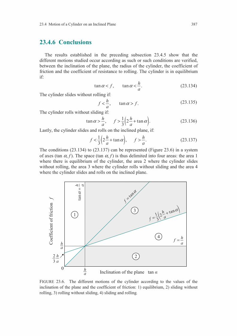
23.4 Motion of a Cylinder on an Inclined Plane 387
1
2
3
4
0Inclination of the plane tan
Co
effi
cien
t o
f fr
icti
on
f
hf
a=
tan
f
α
=
()
1 2tan
3
h
f a
α
=+
ha
2
3
h
a
tan
h aα
=
ha
23.4.6 Conclusions
The results established in the preceding subsection 23.4.5 show that the
different motions studied occur according as such or such conditions are verified,
between the inclination of the plane, the radius of the cylinder, the coefficient of
friction and the coefficient of resistance to rolling. The cylinder is in equilibrium
if:
tan , tan .h
fa
α α< < (23.134)
The cylinder slides without rolling if:
, tan .h
f fa
α< > (23.135)
The cylinder rolls without sliding if:
( )1tan , 2 tan .
3
h hf
a aα α> > + (23.136)
Lastly, the cylinder slides and rolls on the inclined plane, if:
( )12 tan , .
3
h hf f
a aα< + > (23.137)
The conditions (23.134) to (23.137) can be represented (Figure 23.6) in a system
of axes (tan α, f ). The space (tan α, f ) is thus delimited into four areas: the area 1
where there is equilibrium of the cylinder, the area 2 where the cylinder slides
without rolling, the area 3 where the cylinder rolls without sliding and the area 4
where the cylinder slides and rolls on the inclined plane.
FIGURE 23.6. The different motions of the cylinder according to the values of the
inclination of the plane and the coefficient of friction: 1) equilibrium, 2) sliding without
rolling, 3) rolling without sliding, 4) sliding and rolling.
388 Chapter 23 Plane Motion of a Rigid Body
In practice, the coefficient h of resistance to rolling is low and the inequality /f h a> is always satisfied. The motion of sliding of the cylinder without rolling is then not observed and the equilibrium of the cylinder occurs only for very low values of the inclination of the plane.
COMMENTS
The various motions studied in the present chapter make it possible to
highlight how the actions of friction occur in the equilibrium and the
motions of bodies. In the case of a parallelepiped moving on an inclined
plane (Section 23.2), the different types of friction can be considered and
the motion observed depends on the conditions of friction: absence of
friction, viscous friction or dry friction. In contrast, in the case of the
analyses of the motions developed in Sections 23.3 and 23.4, it is necessary
to consider a dry friction between solids to describe the different motions
which are observed. Also, these examples illustrate simply how the laws of
friction interact between solids. The reader will pay a great attention to the
development of the analyses implemented in this chapter.
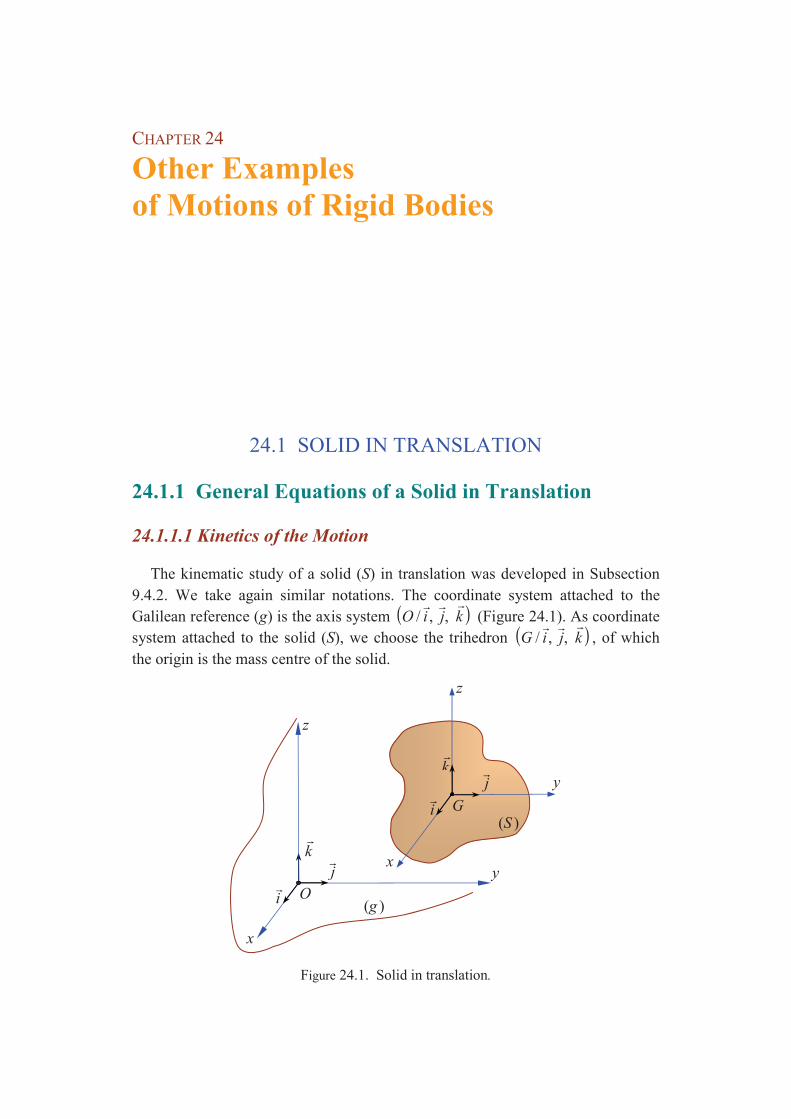
CHAPTER 24
Other Examples of Motions of Rigid Bodies
24.1 SOLID IN TRANSLATION
24.1.1 General Equations of a Solid in Translation
24.1.1.1 Kinetics of the Motion
The kinematic study of a solid (S) in translation was developed in Subsection
9.4.2. We take again similar notations. The coordinate system attached to the
Galilean reference (g) is the axis system ( ) / , ,O i j k
(Figure 24.1). As coordinate
system attached to the solid (S), we choose the trihedron ( ) / , ,G i j k
, of which
the origin is the mass centre of the solid.
Figure 24.1. Solid in translation.
Oi
j
k
y
z
x
jk
i
G(S )
z
y
x
(g )
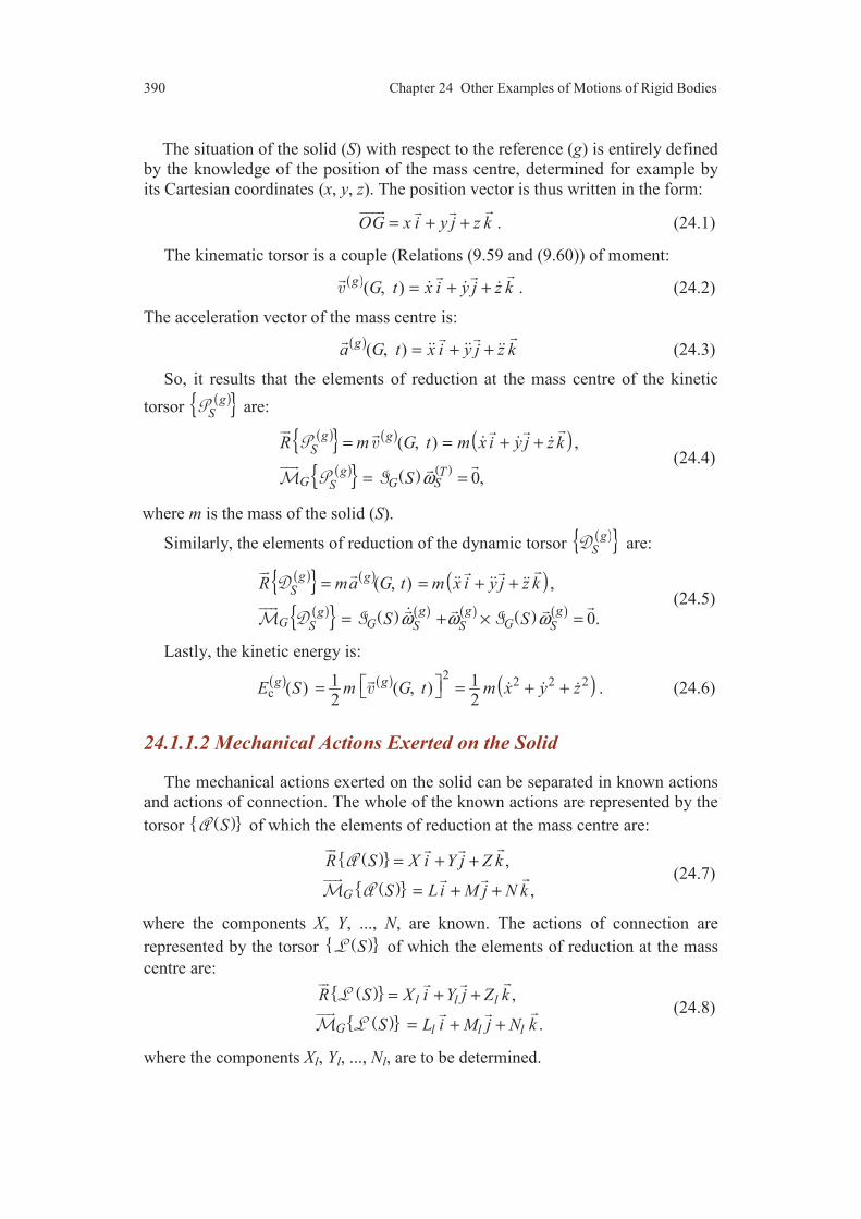
390 Chapter 24 Other Examples of Motions of Rigid Bodies
The situation of the solid (S) with respect to the reference (g) is entirely defined
by the knowledge of the position of the mass centre, determined for example by
its Cartesian coordinates (x, y, z). The position vector is thus written in the form:
OG x i y j z k= + +
. (24.1)
The kinematic torsor is a couple (Relations (9.59 and (9.60)) of moment:
( ) ( , )
gG t x i y j z k= + +
. (24.2)
The acceleration vector of the mass centre is:
( ) ( , )
ga G t x i y j z k= + +
(24.3)
So, it results that the elements of reduction at the mass centre of the kinetic
torsor ( ) g
S are:
( ) ( ) ( )( ) ( ) ( )
( , ) ,
0,
g gS
g TG G SS
R m G t m x i y j z k
S ω
= = + +
= =
(24.4)
where m is the mass of the solid (S).
Similarly, the elements of reduction of the dynamic torsor ( ) g
S are:
( ) ( ) ( )( ) ( ) ( ) ( ) ( ) ( )
( , ) ,
0.
g gS
g g ggG G GS S S S
R ma G t m x i y j z k
S Sω ω ω
= = + +
= + × =
(24.5)
Lastly, the kinetic energy is:
( ) ( ) ( )2
2 2 2c
1 1( ) ( , )2 2
g gE S m G t m x y z = = + +
. (24.6)
24.1.1.2 Mechanical Actions Exerted on the Solid
The mechanical actions exerted on the solid can be separated in known actions
and actions of connection. The whole of the known actions are represented by the
torsor ( ) S of which the elements of reduction at the mass centre are:
( )
( )
,
,G
R S X i Y j Z k
S Li M j N k
= + +
= + +
(24.7)
where the components X, Y, ..., N, are known. The actions of connection are
represented by the torsor ( ) S of which the elements of reduction at the mass
centre are:
( )
( )
,
.
l l l
G l l l
R S X i Y j Z k
S L i M j N k
= + +
= + +
(24.8)
where the components Xl, Yl, ..., Nl, are to be determined.

24.1 Solid in Translation 391
24.1.1.3 Equations Deduced from the Fundamental Principle
The fundamental principle of dynamics applied to the solid in translation is
written as: ( ) ( ) ( ) g
S S S= + . (24.9)
This equation leads to the six scalar equations:
,
,
,
0 ,
0 ,
0 .
l
l
l
l
l
l
mx X X
my Y Y
mz Z Z
L L
M M
N N
= +
= +
= +
= +
= +
= +
(24.10)
We have 6 equations to determine 9 unknowns: the six components of the actions
of connection (Xl, Yl, ..., Nl) and the three parameters of translation (x, y, z). The
physical nature of the connection will allow us to obtain three additional equa-
tions, necessary to determine entirely the problem.
24.1.2 Free Solid in Translation
The case of a free solid in translation, submitted to known actions, can be
deduced from the preceding general equations, by making null the actions of
connection. Equations (24.10) are written in this case:
,
,
,
0, 0, 0.
mx X
my Y
mz Z
L M N
=
=
=
= = =
(24.11)
The first three equations allow us to derive x, y and z as functions of time. These
coordinates determine the motion of the solid. The last three equations express the
fact that the moment of the actions exerted must be null at the mass centre. Hence
the following result: the necessary (but not sufficient) condition in order that a
free body has a motion of translation is that the moment at the mass centre of the
mechanical actions exerted on the body is zero. The mechanical actions exerted
on the body are equivalent to a force of which the support passes through the mass
centre.
An example of such a case is that of a free solid subjected to the action of
gravity and not having a motion of proper rotation: ball without spinning for
example. If the axis Oz
is the upward vertical axis, the three equations of motion
are written:
0, 0, .x y z g= = = (24.12)

392 Chapter 24 Other Examples of Motions of Rigid Bodies
Such a motion was studied in Chapter 7 (Section 7.3): the motion of the mass
centre is a motion with parabolic or rectilinear trajectory. The trajectories of the
other points of the solid are deduced from the trajectory of the mass centre by
translation (Subsection 9.4.2.1).
Lastly, note that the theorem of the kinetic energy (18.24) allows us to obtain
the expression which relates the velocity vectors and the altitudes of the mass
centre for two given positions:
( ) ( ) ( )
2 2
2 12 1( , ) ( , ) 2g g
G t G t g z z − = − − . (24.13)
24.2 MOTION OF A SOLID PLACED
ON A WAGON
24.2.1 Introduction
A parallelepiped (S1) of masse m1 and edges a, b, c is placed on a wagon (S2)
of mass m2. The wagon is animated by a motion of rectilinear translation along the
horizontal axis Ox
, guiding the wagon by rails (Figure 24.2). The parallelepiped
is set so that its mass centre G1 is located in the same vertical plane (Oxy) as the
mass centre G2 of the wagon. It is exerted on the wagon a driving action equi-
valent to a force of horizontal support passing through the mass centre of the
wagon. This action is represented by the torsor ( ) 2S such as:
( ) ( )
2
2
,
0.G
R S F i
S
=
=
(24.14)
FIGURE 24.2. Parallelepiped on a moving chariot.
A B
CD
y
O
I
G2
G1
(S2)
(S1)
y y1
x1
x
x(g)

24.2 Motion of a Solid Placed on a Wagon 393
A
B
C
y
O
G2
G1
(S2)
(S1)
yy1
x1
x
x(g)
D
1 x
According to the values of F, we observe one of the following events when the
wagon is moving: 1) the parallelepiped (S1) stays in equilibrium on the wagon; 2)
the parallelepiped slides on the wagon without rocking; 3) the parallelepiped
rocks around the edge passing through D, without sliding; 4) the parallelepiped
rocks around the edges and slides. We intend to analyse each type of early motion.
24.2.2 Parameters of Situation
The most general motion of the parallelepiped is that of rocking and sliding
(Figure 24.3). To the wagon (S2), we associate the coordinate system (G2xyz), of
fixed orientation with respect to the reference system (Oxyz). The mass centre G2
of the wagon has for coordinates (x2, h, 0) in the system (Oxyz), where the height
h is independent of the position of the wagon. The situation of the wagon is
determined by the only parameter of translation x2. The position vector of G2 is
written:
2 2OG x i h j= +
. (24.15)
To the parallelepiped (S1), we associate the system (Gx1y1z) of axes parallel to the
edges. The situation of the parallelepiped is determined by the coordinates
( )1 1, , 0x y of the mass centre G1 in the system (Oxyz) and by the angle of rotation
ψ1 between the axes Gx
and 1Gx
. The position vector of G1 is written:
1 1 1OG x i y j= +
. (24.16)
Finally, in the most general case of rocking and sliding of the parallelepiped on
the wagon, the parameters of situation are: x1, y1, ψ1 and x2.
FIGURE 24.3. Rocking and sliding of the parallelepiped on the wagon.
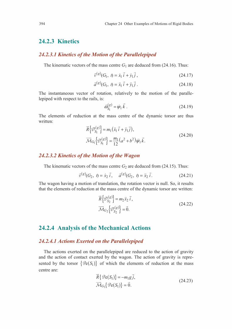
394 Chapter 24 Other Examples of Motions of Rigid Bodies
24.2.3 Kinetics
24.2.3.1 Kinetics of the Motion of the Parallelepiped
The kinematic vectors of the mass centre G1 are deduced from (24.16). Thus:
( ) 1 1 1( , )
gG t x i y j= +
, (24.17)
( ) 1 1 1( , )
ga G t x i y j= +
. (24.18)
The instantaneous vector of rotation, relatively to the motion of the paralle-
lepiped with respect to the rails, is:
( )1
1g
Skω ψ=
. (24.19)
The elements of reduction at the mass centre of the dynamic torsor are thus
written:
( ) ( )
( ) ( )
1
1 1
1 1 1
2 211
,
.12
g
S
gG S
R m x i y j
ma b kψ
= +
= +
(24.20)
24.2.3.2 Kinetics of the Motion of the Wagon
The kinematic vectors of the mass centre G2 are deduced from (24.15). Thus:
( ) ( ) 2 2 2 2( , ) , ( , ) .
g gG t x i a G t x i= =
(24.21)
The wagon having a motion of translation, the rotation vector is null. So, it results
that the elements of reduction at the mass centre of the dynamic torsor are written:
( ) ( )
2
2 2
2 2 ,
0.
g
S
gG S
R m x i=
=
(24.22)
24.2.4 Analysis of the Mechanical Actions
24.2.4.1 Actions Exerted on the Parallelepiped
The actions exerted on the parallelepiped are reduced to the action of gravity
and the action of contact exerted by the wagon. The action of gravity is repre-
sented by the torsor ( ) 1e S of which the elements of reduction at the mass
centre are:
( )
( )
1
1 1
1
e ,
e 0.G
R S m g j
S
= −
=
(24.23)
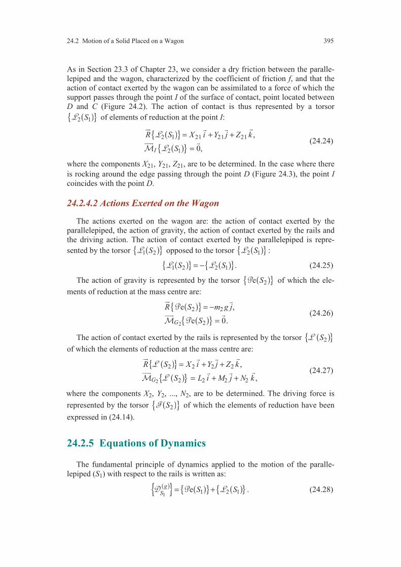
24.2 Motion of a Solid Placed on a Wagon 395
As in Section 23.3 of Chapter 23, we consider a dry friction between the paralle-
lepiped and the wagon, characterized by the coefficient of friction f, and that the
action of contact exerted by the wagon can be assimilated to a force of which the
support passes through the point I of the surface of contact, point located between
D and C (Figure 24.2). The action of contact is thus represented by a torsor
( ) 2 1S of elements of reduction at the point I:
( )
( )
2 1 21 21 21
2 1
,
0,I
R S X i Y j Z k
S
= + +
=
(24.24)
where the components X21, Y21, Z21, are to be determined. In the case where there
is rocking around the edge passing through the point D (Figure 24.3), the point I
coincides with the point D.
24.2.4.2 Actions Exerted on the Wagon
The actions exerted on the wagon are: the action of contact exerted by the
parallelepiped, the action of gravity, the action of contact exerted by the rails and
the driving action. The action of contact exerted by the parallelepiped is repre-
sented by the torsor ( ) 1 2S opposed to the torsor ( ) 2 1S :
( ) ( ) 1 2 2 1 .S S= − (24.25)
The action of gravity is represented by the torsor ( ) 2e S of which the ele-
ments of reduction at the mass centre are:
( )
( )
2
2 2
2
e ,
e 0.G
R S m g j
S
= −
=
(24.26)
The action of contact exerted by the rails is represented by the torsor ( ) 2S
of which the elements of reduction at the mass centre are:
( )
( )
2
2 2 2 2
2 2 2 2
,
,G
R S X i Y j Z k
S L i M j N k
= + +
= + +
(24.27)
where the components X2, Y2, ..., N2, are to be determined. The driving force is
represented by the torsor ( ) 2S of which the elements of reduction have been
expressed in (24.14).
24.2.5 Equations of Dynamics
The fundamental principle of dynamics applied to the motion of the paralle-
lepiped (S1) with respect to the rails is written as:
( ) ( ) ( ) 1
1 2 1eg
SS S= + . (24.28)

396 Chapter 24 Other Examples of Motions of Rigid Bodies
The fundamental principle of dynamics applied to the motion of the wagon
with respect to the rails leads to: ( ) ( ) ( ) ( ) ( ) 2
2 2 1 2 2eg
SS S S S= − + + . (24.29)
Lastly, one of the two equations can be replaced by the equation obtained while
applying the fundamental principle to the set of the two solids. We obtain:
( ) ( ) ( ) ( ) ( ) ( )
1 21 2 2 2e e
g g
S SS S S S+ = + + + . (24.30)
Among these equations, we consider those which will allow us to describe the
different motions observed. Equation (24.28) leads to:
( ) ( ) 1
1 1 21
1 1 1 21
21
2 211 2 1
,
,
0 ,
.12
G
m x X
m y m g Y
Z
ma b Sψ
=
= − +
=
+ =
(24.31)
The last equation has to be expressed while taking account of Relations (24.24).
In this way, we set:
1 1 1G I a i b j= +
, (24.32)
where a1 and b1 depend on the motion. We obtain, considering the relation
21 0Z = :
( ) ( )1 2 1 1 21 1 21G S b X a Y k= − +
. (24.33)
Equation (24.28) leads finally to the equations:
( )
1 1 21
1 1 1 21
21
2 211 1 21 1 21
,
,
0 ,
.12
m x X
m y m g Y
Z
ma b b X a Yψ
=
= − +
=
+ = − +
(24.34)
Also, we shall have to use the equation between the resultants derived from
Equation (24.30). Thus:
( )1 1 2 2 2
1 1 1 2 2
2
,
,
0 .
m x m x X F
m y m m g Y
Z
+ = +
= − + +
=
(24.35)
We shall suppose that the contact between the wagon and the rails occurs without
friction, thus that X2 = 0. The preceding equations are then written:
( )1 1 2 2
1 1 1 2 2
2
,
,
0.
m x m x F
m y m m g Y
Z
+ =
= − + +
=
(24.36)
The first equation will allow us to determine the motion of the wagon, whereas
the second one expresses the vertical component of the resultant of the action of
contact exerted by the rails on the wagon.
24.2 Motion of a Solid Placed on a Wagon 397
24.2.6 Analysis of the Different Motions
24.2.6.1 The Parallelepiped is in Equilibrium on the Wagon
The equilibrium of the parallelepiped on the wagon is characterized by:
1 2 1 1 1, 0, 0, ,2
bx x y bψ= = = = − (24.37)
and Equations (24.34) and (24.36) are written:
( )( )
1 1 21
1 21
21 1 21
1 2 1
1 2 2
,
0 ,
0 .2
,
0 .
m x X
m g Y
bX a Y
m m x F
m m g Y
=
= − +
= +
+ =
= − + +
(24.38)
To these equations, we have to associate the conditions of friction:
21 21 210, Y X f Y> < . (24.39)
From Equations (24.38), we deduce:
( )
1 21 2
121
1 2
21 1
11 2
,
,
,
.2
Fx x
m m
mX F
m m
Y m g
b Fa
m m g
= =+
=+
=
= −+
(24.40)
The condition 21 0Y > is satisfied, and the condition 21 21X f Y< is written:
( )1 2F f m m g< + . (24.41)
Moreover, the point I must be located between the points C and D
1( /2 /2)a a a− < < . It results that, in the case where F is positive, the following
inequality must be satisfied:
( )1 2a
F m m gb
< + . (24.42)
The conditions (24.41) and (24.42) being satisfied, the parallelepiped is in equi-
librium on the wagon. The motion of the parallelepiped-wagon set is imposed by
the force F, in accordance with the first of Equations (24.40).
24.2.6.2 The Parallelepiped Slides on the Wagon without Rocking
The motion is then characterized by:
1 2 1 1 1, 0, 0, .2
bx x y bψ≠ = = = − (24.43)
398 Chapter 24 Other Examples of Motions of Rigid Bodies
Equations (24.34) and (24.36) are written:
( )
1 1 21
21 1
21 1 21
1 1 2 2
2 1 2
,
,
0.2
,
.
m x X
Y m g
bX a Y
m x m x F
Y m m g
=
=
+ =
+ =
= +
(24.44)
To these equations, it is necessary to associate the conditions of friction:
21 21 21 1 2 10, , , .2 2
a aY X f Y x x a> = < − < < (24.45)
Combining Equations (24.44) and (24.45) allows us to determine first the compo-
nents of the action of contact:
21 1 21 1, ,Y m g X fm g= = (24.46)
and then the motions of the parallelepiped and the wagon:
1 22
, .F
x fg x fgm
= = − (24.47)
Sliding of the parallelepiped occurs if the following conditions are satisfied:
( )1 2 , .a
F f m m g fb
> + < (24.48)
24.2.6.3 The Parallelepiped Rocks and Slides on the Wagon
In the case where there is rocking of the parallelepiped (Figure 24.4), this
motion occurs around the edge passing through the point D. The coordinates of
the mass centre G1 can be expressed as functions of the Cartesian coordinates
( )( ), ( ), 0x D y D of the point D as:
( )( )
1 1
1 1
1
( ) cos ,
( ) sin ,
0,
x x D l
y y D l
z
ψ γ
ψ γ
= + +
= + +
=
(24.49)
introducing the geometrical characteristics of the parallelepiped:
2 2 11, tan .
2
al a b
bγ −= + = (24.50)
From this, we deduce then:
( )( )
1 1 1
1 1 1
( ) sin ,
cos ,
x x D l
y l
ψ ψ γ
ψ ψ γ
= − +
= +
(24.51)
and
( ) ( )
( ) ( )
21 1 1 1 1
21 1 1 1 1
( ) sin cos ,
cos sin .
x x D l
y l
ψ ψ γ ψ ψ γ
ψ ψ γ ψ ψ γ
= − + + +
= + − +
(24.52)

24.2 Motion of a Solid Placed on a Wagon 399
A
y
y1
x1
x
D
G1
x(D)
y(D)
(S1)
(S2) wagon
1
FIGURE 24.4. Rocking motion of the parallelepiped.
Moreover:
( ) ( )1 1 1 1cos sinG I G D l i jψ γ ψ γ = = − + + +
(24.53)
For the early motion, we have 1 0ψ ≈ and 1 0ψ ≈ . The preceding expressions
are reduced to:
( )
1 1
1 1
1 1
( ) sin ,
cos ,
cos sin .
x x D l
y l
G I G D l i j
ψ γψ γ
γ γ
= −
=
= = − +
(24.54)
Hence:
1 1cos , sina l b lγ γ= − = − . (24.55)
In the case where the parallelepiped rocks and slides on the wagon, Equations
(24.34) and (24.36) are written for the early motion in the form:
[ ]
[ ]
1 1 21
1 1 1 21
1 1 21 21
1 1 2 2
( ) sin ,
cos ,
sin cos .3
( ) sin .
m x D l X
m l m g Y
lm X Y
m x D l m x F
ψ γ
ψ γ
ψ γ γ
ψ γ
− =
= − +
= −
− + =
(24.56)
To these equations, are associated the conditions of contact:
21 21 21 1 20, , 0, ( ) 0, ( )Y X fY x D x D xψ> = > > < . (24.57)
Solving Equations (24.56) leads to:

400 Chapter 24 Other Examples of Motions of Rigid Bodies
( )
( )
( )
1 2
121 2
21 21
2
2
12 2
2 2
3 sin cos,
1 3cos 3 sin cos
,1 3cos 3 sin cos
,
1 3sin 3sin cos( ) ,
1 3cos 3 sin cos
.1 3cos 3 sin cos
g f
l f
m gY
f
X f Y
fx D g
f
gmFx f
m m f
γ γψ
γ γ γ
γ γ γ
γ γ γ
γ γ γ
γ γ γ
−=
+ −
=+ −
=
+ −=
+ −
= −+ −
(24.58)
The condition 21 0Y > is satisfied if:
21 3cos
3sin cosf
γγ γ
+< . (24.59)
The condition 1 0ψ > leads to:
.b
fa
> (24.60)
Lastly, the conditions ( ) 0x D > and 2( )x D x< are written:
2
3sin cos
1 3sinf
γ γ
γ>
+, (24.61)
and
( )21 2 2
2
1 3sin 3 sin cos.
1 3cos 3 sin cos
f m m mF
f
γ γ γ
γ γ γ
+ + − >+ −
(24.62)
24.2.6.4 The Parallelepiped Rocks without Sliding
In the case where there is not sliding of the point D on the wagon: 2( )x D x=
and Equations (24.56) are written:
( )
( )
1 2 1 21
1 1 1 21
1 1 21 21
1 2 2 1 1
sin ,
cos ,
sin cos ,3
sin .
m x l X
m l m g Y
lm X Y
m m x m l F
ψ γψ γ
ψ γ γ
ψ γ
− =
= − +
= −
+ − =
(24.63)
To these equations, we have to associate the conditions:
21 21 21 1 20, , 0, 0Y X fY xψ> < > > . (24.64)
Solving Equations (24.63), we obtain:
( )
( )1 2
1 21 2
sin cos3,
1 3cos 4
F m m g
l m m
γ γψ
γ
− +=
+ +

24.2 Motion of a Solid Placed on a Wagon 401
( )( )
( )( )
( )
12 2
1 2
21 2
21 1 21 2
22
21 1 21 2
4 3 sin cos,
1 3cos 4
3 sin cos 4 3cos,
1 3cos 4
4 3sin 3 sin cos.
1 3cos 4
F m gx
m m
F m m gY m
m m
F m gX m
m m
γ γ
γ
γ γ γ
γ
γ γ γ
γ
−=
+ +
+ + − =+ +
− +=
+ +
(24.65)
The condition 1 0ψ > leads to:
( )1 2b
F m m ga
> + . (24.66)
The condition 2 0x > is written:
13
sin cos4
F m g γ γ> . (24.67)
The condition 21 0Y > is always satisfied. Lastly, the condition 21 21X fY< leads
to the inequality:
( )21 2 2
2
4 3cos 3 sin cos
4 3sin 3 sin cos
f m m mF g
f
γ γ γ
γ γ γ
+ − − <− −
. (24.68)
24.2.6.5 Conclusions on the Analysis of the Different Motions
The different motions studied take place according as such or such of the con-
ditions (24.41), (24.42), (24.48), (24.59) to (24.62), (24.66) to (24.68) are
satisfied. Thus, the different motions occur according to the values of the edges of
the parallelepiped, of the resultant of the driving force, of the masses of the paral-
lelepiped and wagon, of the coefficient of friction.
As an example, we examine the case of a parallelepiped with a square section,
for which:
1, sin cos ,
2a b γ γ= = = (24.69)
and with a mass equal to that of the wagon: 1 2m m= . The conditions obtained are
written as follows:
— Equilibrium of the parallelepiped on the wagon:
1 12 , 2F fm g F m g< < . (24.70)
— Sliding without rocking of the parallelepiped:
12 , 1F fm g f> < . (24.71)
— Rocking and sliding of the parallelepiped:
17 35
1 , 3 5 3
ff F m g
f
−< < >
−. (24.72)

402 Chapter 24 Other Examples of Motions of Rigid Bodies
FIGURE 24.5. The different motions of the parallelepiped according to the values of the
driving force and the coefficient of friction.
— Rocking without sliding of the parallelepiped:
1 17 3
2 , 5 3
fF m g F m g
f
−> <
−. (24.73)
The conditions (24.70) to (24.73) can be represented graphically (Figure 24.5) in a
system of axes (F, f ). The space (F, f ) is thus delimited into four areas: the area 1
where there is equilibrium of the parallelepiped on the wagon, the area 2 where
the parallelepiped slides without rocking, the area 3 where the parallelepiped
rocks and slides and the area 4 where the parallelepiped rocks without sliding.
24.3 COUPLED MOTIONS OF TWO SOLIDS
24.3.1 Introduction
We consider the simple mechanical system schematized in Figure 24.6. The
solid (S1) of mass m1 is connected to the support (T) through a prismatic conne-
ction (not represented in the figure) of horizontal axis (∆1). The solid is subjected
to the action of the spring (R) of negligible mass, of axis (∆1), stiffness k and length
l0 in the absence of action exerted on the spring. A solid (S2) of mass m2 is
connected to the solid (S1) using a hinge connection of horizontal axis (∆2),
passing through the mass centre G1 of the solid (S1) and orthogonal to the axis
(∆1). The point of the connection of the spring with (S1) is located at a distance d
from the mass centre G1. Lastly, the mass centre G2 of the solid (S2) moves in the
vertical plane passing through G1. It is located at a distance a from G1.
1
2
3
4
1
5/3
3/7
12m g0Driving force F
Co
effi
cien
t o
f fr
icti
on
f
1f =
12
Fm
g=
1
2
F
fmg
=
( ) ( ) 1
5 37 3
f F f m g
−= −

24.3 Coupled Motions of Two Solids 403
FIGURE 24.6. System of two coupled solids.
24.3.2 Parameters of Situation and Kinematics
We choose the coordinate system (Oxyz) attached to the support such that the
origin O coincides with the point of connection of the spring with the support, and
such that the axis Oy
coincides with the axis of the spring and that the axis Ox
is
downward vertical.
24.3.2.1 Motion of the Solid (S1) with respect to the Support (T)
As coordinate system attached to the solid (S1), we choose the trihedron
(G1xyz) of invariable orientation with respect to the support. The motion of the
solid (S1) is a motion of rectilinear translation characterized by the abscissa y of
the mass centre G1 along the axis 1G y
.
The kinematic torsor ( ) 1
TS of the motion of the solid (S1) with respect to the
support has for elements of reduction at G1:
( ) ( )
( ) ( )
1 1
1 11
0,
( , ) .
T TS S
T TG S
R
G t y j
ω= =
= =
(24.74)
24.3.2.2 Motion of the Solid (S2) with respect to the Support (T)
As coordinate system attached to the solid (S2), we choose the trihedron
( )1 2 2G x y z , such that the axis 1 2G x
passes through the mass centre G2 of the solid
(S2). The situation of the solid (S2) with respect to the solid (S1) is characterized
by the angle of rotation ψ between the axes 1G x
and 1 2G x
. The basis change is
written:
(T) (R) (S1)
(S2)
G2
G1 (1)
(2) y
x
x x2
y2
z
z
d
O
a

404 Chapter 24 Other Examples of Motions of Rigid Bodies
2
2
cos sin ,
sin cos .
i i j
j i j
ψ ψ
ψ ψ
= +
= − +
(24.75)
The kinematic torsor ( ) 2
TS relative to the motion of the solid (S2) with respect
to the support has for elements of reduction at the point G1:
( ) ( )
( ) ( )
2 2
1 21
,
( , ) .
T TS S
T TG S
R k
G t y j
ω ψ= =
= =
(24.76)
The velocity vector of the mass centre G2 is:
( ) ( ) ( )
222 1 1 2( , ) ( , )T T T
SG t G t G G y j a jω ψ= + × = +
. (24.77)
The acceleration vector of the mass centre is obtained by deriving the preceding
expression with respect to time. We obtain:
( )
22 2 2( , )Ta G t y j a j a iψ ψ= + −
, (24.78)
or by taking account of Relation (24.75) of basis change:
( ) ( ) ( )
2 22( , ) cos sin cos sinTa G t a i y a jψ ψ ψ ψ ψ ψ ψ ψ = − + + + −
. (24.79)
24.3.3 Kinetics
24.3.3.1 Motion of the Solid (S1)
The kinetic torsor ( ) 1
TS relative to the motion of the solid (S1) with respect to
the support has for elements of reduction at the mass centre G1:
( ) ( )
( ) ( ) ( )
1
1 11 1
1 1 1
1
( , ) ,
0.
T TS
T TG GS S
R m G t m y j
S ω
= =
= =
(24.80)
The kinetic energy is deduced easily from (24.74) and (24.80). Thus:
( ) 2c 1 1
1( )
2TE S m y= . (24.81)
Lastly, the dynamic torsor ( ) 1
TS relative to the motion of the solid (S1) with
respect to the support has for elements of reduction at the mass centre G1:
( ) ( )
( ) ( ) ( ) ( ) ( ) ( )
1
1 1 11 1 1 1
1 1 1
1 1
( , ) ,
0.
T TS
T T T TG G GS S S S
R m a G t m y j
S Sω ω ω
= =
= + × =
(24.82)

24.3 Coupled Motions of Two Solids 405
24.3.3.2 Motion of the Solid (S2)
The kinetic torsor ( ) 2
TS relative to the motion of the solid (S2) with respect to
the support has for elements of reduction at the point G1:
( ) ( ) ( )( ) ( ) ( ) ( )
2
1 12 2
2 2 2 2
22 1 1 2
( , ) ,
( , ) .
T TS
T T TG GS S
R m G t m y j a j
m G G G t S
ψ
ω
= = +
= × +
(24.83)
The operator of inertia at the point G1 of the solid (S2) is represented, in the
basis (2) = ( )2 2, , i j k
attached to the solid, by the matrix of inertia:
( )
1
2 2 22
2 2 2 2
2 2 2
( )G
A F E
S F B D
E D C
− − = − − − −
I . (24.84)
The moment at the point G1 of the kinetic torsor is thus written by expressing
(24.83) in the form: ( ) ( )
1 22 2 2 2 2 2 cosT
G SE i D j C m ay kψ ψ ψ ψ= − − + +
. (24.85)
The kinetic energy is calculated by the relation:
( ) ( ) ( ) 2 2
c 21
( )2
T T TS S
E S = ⋅ . (24.86)
Taking account of Expressions (24.76), (24.83) and (24.85), we obtain:
( ) 2 2c 2 2 2 2
1 1( ) cos
2 2TE S m y C m a yψ ψ ψ= + + . (24.87)
The total kinetic energy associated to the motions of the two solids is obtained
by adding Expressions (24.81) and (24.87). Thus:
( )( ) ( ) 2 2c 1 2 1 2 2 2
1 1cos
2 2TE S S m m y C m a yψ ψ ψ∪ = + + + . (24.88)
The first term represents the kinetic energy of translation of the two solids, the
second term the kinetic energy of rotation of the solid (S2) and the third term is a
coupling kinetic energy.
The dynamic torsor ( )
2
TS relative to the motion of the solid (S2) with respect
to the support has for elements of reduction at the point G1:
( ) ( ) ( )( ) ( ) ( ) ( ) ( ) ( ) ( )
2
1 1 12 2 2 2
22 2 2 2 2
22 1 1 2 2
( , ) ,
( , ) .
T TS
T T T T TG G GS S S S
R m a G t m y j a i a j
m G G a G t S S
ψ ψ
ω ω ω
= = − +
= × + + ×
(24.89)
The resultant will be expressed in the basis ( ), , i j k
by considering the basis
change given by Relation (24.75). Introducing the matrix of inertia (24.84) in

406 Chapter 24 Other Examples of Motions of Rigid Bodies
the expression of the moment, we obtain:
( ) ( ) ( ) ( )
1 2
2 22 2 2 2 2 2 2 2 cosT
G SE D i D E j C m ay kψ ψ ψ ψ ψ ψ= − + − + + +
(24.90)
The moment can then be expressed in the basis ( ), , i j k
using Relation (24.75)
of basis change. We obtain:
( ) ( ) ( )
( ) ( )( )
1 2
2 22 2 2 2
2 22 2 2 2
2 2
cos sin
sin cos
cos .
TG S
E D D E i
E D D E j
C m ay k
ψ ψ ψ ψ ψ ψ
ψ ψ ψ ψ ψ ψ
ψ ψ
= − + + +
+ − + − +
+ +
(24.91)
24.3.4 Analysis of the Mechanical Actions
24.3.4.1 Actions Exerted on the Solid (S1)
The mechanical actions exerted on the solid (S1) are: the action of gravity, the
action of the spring, the action of the support induced by the prismatic connection
and the action of the solid (S2) induced by the hinge connection.
The action of gravity is represented by the torsor ( ) 1e S of elements of
reduction at the mass centre:
( )
( )
1
1 1
1
e ,
e 0.G
R S m g i
S
=
=
(24.92)
The power developed by the action of gravity in the reference attached to the
support is: ( ) ( ) ( ) ( )
11 1e e 0T T
SP S S= =⋅ . (24.93)
The action exerted by the spring is a force of axis (∆1), represented by the
torsor 1( )S and of which the elements of reduction at the point G1 are:
( )
1
1 0
1
( ) ,
( ) 0.G
R S k y d l i
S
= − − −
=
(24.94)
The power developed by the action of the spring is:
( ) ( ) ( )1
1 1 0( ) ( )T TS
P S S k y d l y= = − − −⋅ . (24.95)
The action exerted by the support through the prismatic connection is repre-
sented by the torsor 1( )S . Its elements of reduction at the point G1 are:
1
1 1 1 1
1 1 1 1
( ) ,
( ) .G
R S X i Y j Z k
S L i M j N k
= + +
= + +
(24.96)

24.3 Coupled Motions of Two Solids 407
The components X1, Y1, ..., N1, are to be determined. The power developed by the
action of connection is:
( ) ( ) 1
1 1 1( ) ( )T TS
P S S Y y= =⋅ . (24.97)
The action exerted by the solid (S2) through the hinge connection is represented
by the torsor 2 1( )S , of which the elements of reduction at the point G1 are:
1
2 1 21 21 21
2 1 21 21 21
( ) ,
( ) .G
R S X i Y j Z k
S L i M j N k
= + +
= + +
(24.98)
The components X21, Y21, ..., N21, are to be determined. The power developed by
the action of connection exerted by the solid (S2), power evaluated in the refe-
rence (T), is:
( ) ( ) 1
2 1 2 1 21( ) ( )T TS
P S S Y y= =⋅ . (24.99)
24.3.4.2 Actions Exerted on the Solid (S2)
The mechanical actions exerted on the solid (S2) are reduced to the action of
gravity and the action of the solid (S1) induced by the hinge connection.
The action of gravity is represented by the torsor ( ) 2e S of elements of
reduction at the mass centre:
( )
( )
2
2 2
2
e ,
e 0.G
R S m g i
S
=
=
(24.100)
We shall need the moment vector at the point G1. It is written:
( ) ( ) 1 12 2 2 2e e sinG S R S G G m ga kψ= × = −
. (24.101)
The power developed by the action of gravity, evaluated in the reference (T), is:
( ) ( ) ( ) ( )
22 2 2e e sinT T
SP S S m gaψ ψ= = −⋅ . (24.102)
The action exerted by the solid (S2) induced by the hinge connection is repre-
sented by the torsor 1 2( )S opposed to the torsor 2 1( )S :
1 2 2 1( ) ( )S S= − . (24.103)
The power developed by this action, evaluated in the reference (T), is:
( ) ( ) 2
1 2 1 2 21 21( ) ( )T TS
P S S Y y N ψ= = − −⋅ . (24.104)
408 Chapter 24 Other Examples of Motions of Rigid Bodies
24.3.5 Equations Deduced from the Fundamental Principle of Dynamics
24.3.5.1 Motion of the Solid (S1)
In the case where the support is a pseudo-Galilean support (support attached to
the Earth), the fundamental principle of dynamics applied to the motion of the
solid (S1) with respect to the support is written as:
( ) ( ) 1
1 1 1 2 1e ( ) ( ) ( )TS
S S S S= + + + . (24.105)
The vector equations of the resultant and moment at the point G1 lead to the six
scalar equations:
( )1 1 21
1 0 1 21
1 21
1 21
1 21
1 21
0 ,
,
0 ,
0 ,
0 ,
0 .
m g X X
m y k y d l Y Y
Z Z
L L
M M
N N
= + +
= − − − + +
= +
= +
= +
= +
(24.106)
24.3.5.2 Motion of the Solid (S2)
The fundamental principle of dynamics applied to the motion of the solid (S2)
with respect to the support is written:
( ) ( ) 2
2 2 1e ( )TS
S S= − . (24.107)
The vector equations of the resultant and moment at the point G1 lead to the six
scalar equations:
( )
( )
( ) ( )( ) ( )
22 2 21
22 21
21
2 22 2 2 2 21
2 22 2 2 2 21
2 2 21 2
cos sin ,
cos sin ,
0 ,
cos sin ,
sin cos ,
cos sin .
m a m g X
m y a Y
Z
E D D E L
E D D E M
C m a y N m ga
ψ ψ ψ ψ
ψ ψ ψ ψ
ψ ψ ψ ψ ψ ψ
ψ ψ ψ ψ ψ ψ
ψ ψ ψ
− + = −
+ − = −
=
− + + + = −
− + − + = −
+ = − −
(24.108)
24.3.5.3 Motion of the Set of the Two Solids
The fundamental principle of dynamics can be applied to the set constituted of
the two solids. It is then written:

24.3 Coupled Motions of Two Solids 409
( ) ( ) ( ) ( )
1 21 1 1 2e ( ) ( ) eT T
S SS S S S+ = + + + . (24.109)
This equation results from the addition of the two equations (24.105) and
(24.107). In the case where the moments of the torsors are expressed all at the
point G1 (and only in this case), the six scalar equations deduced from (24.109)
are the result of the addition of Equations (24.106) and (24.108). We obtain:
( ) ( )
( ) ( ) ( )
( ) ( )( ) ( )
22 1 2 1
21 2 2 0 1
1
2 22 2 2 2 1
2 22 2 2 2 1
2 2 1 2
cos sin ,
cos sin ,
0 ,
cos sin ,
sin cos ,
cos sin .
m a m m g X
m m y m a k y d l Y
Z
E D D E L
E D D E M
C m a y N m ga
ψ ψ ψ ψ
ψ ψ ψ ψ
ψ ψ ψ ψ ψ ψ
ψ ψ ψ ψ ψ ψ
ψ ψ ψ
− + = + +
+ + − = − − − +
=
− + + + =
− + − + =
+ = −
(24.110)
The components of the action of connection exerted between the two solids do not
appear in these equations. This property is general. The fundamental principle
applied to a set of solids does not introduce the actions exerted between the solids
of this set.
24.3.6 Analysis of the Equations Deduced from the Fundamental Principle
24.3.6.1 Introduction
The fundamental principle of dynamics leads to 12 independent equations
chosen among Equations (24.106), (24.108), (24.110) or possibly among the
linear combinations of these equations. We have 14 unknowns to determine: X1,
Y1, ..., N1, X21, Y21, ..., N21, y and ψ. The physical nature of the actions of
connection will supplement to 14 the number of the equations. Solving the
selected equations will then make it possible to derive the parameters of situation
y and ψ as functions of time, then the components of connection.
24.3.6.2 Case of Connections without Friction
In the case where the connections are frictionless, the power developed by the
actions of connections are zero. For the prismatic connection, Relation (24.97)
leads to:
1 0Y = . (24.111)
An important point must be underlined for the hinge connection. Indeed, one
should not consider the powers (24.99) or (24.104) calculated with respect to the
support. The connection is made between the solids (S1) and (S2) and the power

410 Chapter 24 Other Examples of Motions of Rigid Bodies
to be considered is, for example, the power developed by the action exerted by the
solid (S1) on the solid (S2) and expressed in a reference attached to (S1). The
power developed is written:
( ) ( ) 1 1
21 2 1 2( ) ( )
S S
SP S S= ⋅ , (24.112)
where the kinematic torsor relative to the motion of the solid (S2) with respect to
the solid (S1) is expressed as:
( ) ( ) ( ) 1
2 2 1
S T TS S S
= − . (24.113)
Combining Relations (24.99), (24.103), (24.104), (24.112) and (24.113) leads to:
( ) ( ) ( ) 11 2 1 2 2 1 21( ) ( ) ( )
S T TP S P S P S N ψ= + = − . (24.114)
We find the usual expression of the power developed by the action induced by a
hinge connection. In the absence of friction, we have:
21 0N = . (24.115)
The equations of motion are among Equations (24.106), (24.108) and (24.110)
those which introduce only the components of connections Y1 and N21. Thus, the
second equation (24.110) relative to the motion of the set of the two solids
(component along j
of the resultant) and the sixth equation (24.108) relative to
the motion of the solid (S2) (component along k
of the moment at the point G1):
( ) ( ) ( )21 2 0 2
2 2 2
cos sin 0,
cos sin 0.
m m y k y d l m a
m ay C m ga
ψ ψ ψ ψ
ψ ψ ψ
+ + − − + − =
+ + =
(24.116)
Solving these equations will allow us to obtain y and ψ as functions of time. The
components of the actions of connections will be then deduced from Equations
(24.108) and (24.110).
The equilibrium of the system is obtained when 0,y ψ ψ= = = what leads to:
0 , sin 0 ( 0 ou ).y l d ψ ψ π= + = = (24.117)
The equilibrium corresponding to ψ π= is unstable. In practice, the analytical
resolution of Equations (24.116) is not possible when ψ is arbitrary. It is then
necessary to use a numerical method (Chapter 27).
In the case of low values of ψ around the position of stable equilibrium 0ψ = ,
such as cos 1ψ ≈ and sinψ ψ≈ , Equations (24.116) are written in the form:
( ) ( ) ( )21 2 0 2
2 2 2
0,
0.
m m y k y d l m a
m ay C m ga
ψ ψ ψ
ψ ψ
+ + − − + − =
+ + =
(24.118)
The equations of motion are linearized, and an analytical solution can be obtained
(Subsection 27.5.2 of Chapter 27).

Exercises 411
24.3.6.2 Case of Connections with Viscous Friction
In the case of connections with viscous friction, we have:
1 21, ,t rY c y N c ψ= − − = − (24.119)
where ct and cr are the respective coefficients of friction of the prismatic con-
nection and of the hinge connection. Equations (24.116) of motion are then mo-
dified as:
( ) ( ) ( )21 2 0 2
2 2 2
cos sin 0,
cos sin 0,
t
r
m m y c y k y d l m a
m ay C c m ga
ψ ψ ψ ψ
ψ ψ ψ ψ
+ + + − − + − =
+ + + =
(24.120)
or in linearized form:
( ) ( ) ( )21 2 0 2
2 2 2
0,
0.
t
r
m m y c y k y d l m a
m ay C c m ga
ψ ψ ψ
ψ ψ ψ
+ + + − − + − =
+ + + =
(24.121)
EXERCISES
24.1 Analysis of the motion of two solids (Figure 24.7)
The solid (S1) is a hollowed cylinder in motion of rotation with respect to a
support (T) about a horizontal axis (1). A cylinder (S2) is connected to the cylin-
der (S1) through a traction-compression and torsion spring. The solid (S2) has thus
a motion of translation along the axis of the cylinder (S1) and a motion of rotation
about this axis.
Study the motion of the two solids.
FIGURE 24.7. Motion of two solids.
(S1)
(S2)
(1)

412 Chapter 24 Other Examples of Motions of Rigid Bodies
(T)
(S1)
G1
(1)
(2)
(S2) G2
(M1
(M2
24.2 Study of the motion a radar antennaFor the analysis of its motion, a radar antenna can be considered (Figure 24.8)
as being constituted of a support (S1) and a reflector (S2).
The support (S1) is connected through a hinge connection of vertical axis (1)
with the frame (T) attached to the Earth, using an electric motor (M1). The stator
of the motor is attached to the frame and the rotor is rigidly locked with (1).
The reflector (S2) has a cylindrical symmetry. It is connected through a hinge
connection of horizontal axis (2) with the support (S1), using a motor (M2). The
stator of the motor is attached to the support (S1) and the rotor is rigidly locked
with (2). The mass centre G2 of (S2) is located at the intersection of (1) and (2).
The mass centre G1 of the set constituted of the support (S1) and the stator of
the motor (M2) is located on the axis (1) and the matrix of inertia is arbitrary.
Study the motion of the antenna.
FIGURE 24.8. Radar antenna.
COMMENTS
The motions studied in the present chapter come in complement of the
examples of motions already studied in the preceding chapters. They cons-
titute simple illustrations of the analysis of dynamics of rigid bodies and
they do not call particular comments.
The two exercises will allow the reader to apply the process of the ana-
lysis of dynamics to two simple cases.

Commentaires 413

CHAPTER 25
The Lagrange Equations
25.1 GENERAL ELEMENTS
25.1.1 Free Body and Connected Body
In the case of a solid (S) free with respect to a reference (T), the situation of the
solid is determined by the knowledge of:
— the position of the mass centre G with respect to the reference (T), charac-
terized by three parameters of translation p1, p2, p3 (Cartesian, cylindrical or
spherical coordinates, etc.);
— the orientation of a coordinate system attached to the solid (S) with respect to the reference (T), characterized by the three Eulerian angles ψ, θ, ϕ which we denote by Qi ( 1 ,Q ψ= 2Q θ= and 3Q ϕ= ).
The situation of the solid is determined by the six parameters (p1, p2, p3, Q1,
Q2, Q3), which we denote by the general form qi ( 1 to 6i = ).
In the case where the solid (S) is connected in the reference (T), the situation of
the solid is determined by the position of a particular point P of the solid, cha-
racterized by the parameters of translation pj ( 3j ≤ ), and by the orientation of the
solid (S), characterized by the angles of rotation Qk ( 3k ≤ ). The set of the para-
meters of situation will be also denoted by qi, with 6i < .
25.1.2 Partial Kinematic Torsors
In the case of a solid (S) free in the reference (T), the kinematic torsor, relative
to the motion of the solid, has for elements of reduction at the mass centre:
( ) ( )
( ) ( )( ) ( ) ( )
3
1 2 31 2 3
,
( , ) ,
T TS S S
T T TT T
G S
R k i k
G t p OG p OG p OGp p p
ω ψ θ ϕ= = + +
∂ ∂ ∂= = + +
∂ ∂ ∂
(25.1)
414 Chapitre 25 The Lagrange Equations
where O is a point of reference attached to the reference (T).
The preceding expressions show that the kinematic torsor can be expressed in
the form of a linear combination of torsors as:
( ) ( ) 6
,
1i
T TS i S q
i
q
=
= , (25.2)
where the elements of reduction at the point G of the torsors ( ) , i
TS q are defined in
the following way:
( ) ( )
( )
( ) ( )
( )
( ) ( )
( )
1
2
3
,,1
, 3,2
,,3
0, , , 0 ,
0, , , 0 ,
0, , , 0 .
TT T
S GS p GGG
TT T
S GS p GGG
TT T
S S GS p GGG
OG kp
OG ip
OG kp
ψ
θ
ϕ
∂= =
∂
∂= =
∂
∂= =
∂
(25.3)
The torsors ( ) , i
TS q thus introduced are called the partial kinematic torsors rela-
tive to the respective parameters qi of situation.
Relation (25.2) is transposed to the case of a connected solid, of which the
situation is defined by p parameters, in the form:
( ) ( ) ,
1i
pT T
S i S q
i
q
=
= , (25.4)
where the partial kinematic torsors are characterized by their elements of reduc-
tion at the point P, where the parameters of translation have been defined. If the
parameter qi is the parameter of translation pj, the elements of reduction of the
partial kinematic torsor are:
( ) ( ) ( )
, ,0,
i j
TT T
S q S pP P j P
OPp
∂= = ∂
. (25.5)
If the parameter qi is the parameter of rotation Qk, we shall have:
( ) ( )
, ,, 0
i k
T Tk PS q S QP P
u= =
(25.6)
with
3
, si ,
, si ,
, si .
k
k k
S k
k Q
u i Q
k Q
ψ
θ
ϕ
=
= =
=
(25.7)
25.1 General Elements 415
25.1.3 Power Coefficients
The power developed in the reference (T) by the mechanical action exerted on
the solid (S) and represented by the torsor ( ) S is written from Relation (11.13):
( ) ( ) ( ) ( ) T TSP S S= ⋅ . (25.8)
Taking account of Expressions (25.2) and (25.4), we may write the power in the
form:
( ) ( ) ( ) ( ) 1
i
pT T
qi
i
P S q P S
=
= , (25.9)
setting:
( ) ( ) ( ) ( ) ,i i
T Tq S q
P S S= ⋅ . (25.10)
The coefficient ( ) ( ) i
TqP S thus introduced is called power coefficient relative to
the variable qi.
The power coefficients can be derived from Relation (25.10), requiring to
express the partial kinematic torsors as a preliminary. Usually, they can be obtain-
ned more simply while implementing a direct calculation of the power using
Relation (25.8). The expression obtained then displays the power coefficients.
25.1.4 Perfect Connections
In the case where the solid (S) is connected in the reference (T) through a
connection, the reference (T) exerts an action of connection represented by the
torsor ( ) T S . The connection is perfect if the power developed is zero:
( ) ( ) ( ) ( ) 0T TT T SP S S= =⋅ , (25.11)
what leads, taking account of (25.9), to p relations:
( ) ( ) ( ) ( ) ,
0, 1, 2, . . . , .i i
T Tq T T S q
P S S i p= = =⋅ (25.12)
In the case where the connection cannot be regarded as perfect, it is necessary
to consider hypotheses on the physical nature of the friction processes induced.
The model of viscous friction is the simplest one to implement. This model leads
to write the power coefficients in the form:
( ) ( ) i
Tq T i iP S c q= − (25.13)
where ci is the viscous damping coefficient relative to the parameter of situation qi.

416 Chapitre 25 The Lagrange Equations
25.2 LAGRANGE EQUATIONS RELATIVE TO
A RIGID BODY
25.2.1 Introduction to the Lagrange Equations
We consider the case of a solid (S) in motion relatively to the reference (T). The
kinetic energy relative to the motion of the solid (S) with respect to the reference
(T) can be put in the form (16.27):
( ) ( ) ( ) ( ) ( )2
c1 1( ) ( , )2 2
T T T TS G SE S m G t Sω ω = + ⋅
. (25.14)
We search for expressing in this subsection the expression:
( )( ) ( )( )c c
d
dT T
i i
E S E St q q
∂ ∂−
∂ ∂. (25.15)
Deriving the first term of Expression (25.14) with respect to the variable ,iq
we obtain:
( ) ( ) ( )
21 ( , ) ( , ) ( , )2
T T T
i i
m G t m G t G tq q∂ ∂ = ∂ ∂
⋅
. (25.16)
Then deriving this expression with respect to time, we have:
( )( )
( ) ( ) ( )( )
( )
21 d ( , )2 d
d( , ) ( , ) ( , ) ( , ) .d
TT
i
TT T T T
i i
m G tt q
ma G t G t m G t G tq t q
∂ = ∂
∂ ∂+∂ ∂
⋅ ⋅
(25.17)
To calculate the derivative of the second term, we represent the operator of
inertia by the matrix of inertia at the point G in the principal basis (bS) of inertia:
( )( )
0 0
0 0
0 0
SbG
A
S B
C
=
I . (25.18)
If ω1, ω2 and ω3 are the components of the rotation vector ( )TSω
in the basis (bS),
the second term of Expression (25.14) of the kinetic energy is written:
( ) ( ) ( ) ( )2 2 21 2 3
1 12 2
T TS G SS A B Cω ω ω ω ω= + +⋅ . (25.19)
Deriving this expression with respect to the variable ,iq we obtain:
( ) ( ) ( ) 31 21 2 3
12
T TS G S
i i i i
S A B Cq q q q
ωω ωω ω ω ω ω
∂∂ ∂∂ = + + ∂ ∂ ∂ ∂⋅
, (25.20)
or

25.2 Lagrange Equations Relative to a Rigid Body 417
( ) ( ) ( )( ) ( )
( ) ( )12
S TT T TS
S G S G Si i
S Sq q
ωω ω ω
∂∂ = ∂ ∂⋅ ⋅
. (25.21)
Deriving this expression with respect to time, we obtain:
( )( ) ( ) ( )
( ) ( ) ( )
( ) ( )( ) ( ) ( )
( ) ( )
1 d2 d
d d .d d
TT T
S G Si
S T S TT TT TS S
G S G Si i
St q
S St q q t
ω ω
ω ωω ω
∂ = ∂
∂ ∂ + ∂ ∂
⋅
⋅ ⋅
(25.22)
Implementing a calculation similar to the preceding one, but substituting the
variable iq for the variable qi, we obtain:
( )( ) ( )( )
( )( )
( ) ( ) ( ) c ( , ) ( , ) .
T ST T T T T
S G Si i i
E S m G t G t Sq q q
ω ω∂ ∂ ∂= +∂ ∂ ∂
⋅ ⋅
(25.23)
Combining Expressions (25.17), (25.22) and (25.23) leads, taking account of
Relations (A.25.19) and (A.25.24) of the appendix to this chapter, to the result:
( )( ) ( )( )
( ) ( )
( )( )
( ) ( )
c cd
d
( , ) ,
T T
i i
T ST T T T
GS S Si i
E S E St q q
R G tq q
ω
∂ ∂− =
∂ ∂
∂ ∂+
∂ ∂⋅ ⋅
(25.24)
while introducing the elements of reduction at the point G of the dynamic torsor.
From Relations (25.1) to (25.3), the elements of reduction at the point G of the
partial kinematic torsors are:
( ) ( )
( )
( ) ( )
( )
,
,
,
( , ) .
i
i
ST T
SS qi
TT T
G S qi
Rq
G tq
ω∂=
∂
∂=
∂
(25.25)
Relation (25.24) is thus written finally:
( )( ) ( )( ) ( ) ( ) c c ,
d
d i
T T T TS S q
i i
E S E St q q
∂ ∂− =
∂ ∂⋅
. (25.26)
25.2.2 Lagrange Equations
If the reference (T) is a Galilean reference (g), the fundamental principle of
dynamics leads to:
( ) ( ) ( ) ( ) ( ) ( ) , , ii i
g g g gqS S q S q
S P S= =⋅ ⋅ , (25.27)
where ( ) S is the torsor representing the whole of the actions exerted on the
solid (S) and expressed in the Galilean reference (g). The association of Relations
418 Chapitre 25 The Lagrange Equations
(25.26) and (25.27) leads to the equations:
( )( ) ( )( ) ( ) ( ) c cd
, 1, 2, . . . , ,d i
gg gq
i i
E S E S P S i pt q q
∂ ∂− = =
∂ ∂ (25.28)
where the power coefficients are expressed in the Galilean reference:
( ) ( ) ( ) ( ) ,i i
ggq S qP S S= ⋅ . (25.29)
Equations (25.28) are known under the name of Lagrange equations. They can be
rewritten while distinguishing between the known actions ( ) S exerted on the
solid and the actions of connection ( ) S . Thus:
( )( ) ( )( ) ( ) ( ) ( ) ( )
c cd
,d
1, 2, . . . , ,
i i
g gg gq q
i i
E S E S P S P St q q
i p
∂ ∂− = +
∂ ∂
=
(25.30)
with
( ) ( ) ( ) ( ) ( ) ( ) ( ) ( )
,
,
,
.
i i
i i
ggq S q
ggq S q
P S S
P S S
=
=
⋅
⋅
(25.31)
The Lagrange equations are derived from the fundamental principle of dyna-
mics, and consequently they do not bring any new information compared to the
scalar equations deduced from the fundamental principle. Indeed, the Lagrange
equations are linear combinations of these last equations. Their interest lies in the
fact that they constitute p differential equations of the motion of the solid (S).
Indeed, once determined the physical nature of the connections, Equations (25.30)
form a system of p differential equations where the only unknowns are the p
parameters of situation qi. Solving this system allows us to determine these para-
meters as functions of time. Note however that the determination of the compo-
nents of the actions of connections, other than those appearing in (25.31), requires
to return to the equations derived from the fundamental principle of dynamics.
In the case of frictionless connections, the power coefficients relative to the
actions of connections are zero, and the Lagrange equations (25.30) are reduced
to:
( )( ) ( )( ) ( ) ( ) c cd
, 1, 2, . . . , .d i
gg gq
i i
E S E S P S i pt q q
∂ ∂− = =
∂ ∂ (25.32)
25.2.3 Case where the Mechanical Actions Admit a Potential Energy
In the case where the mechanical actions exerted on the solid, other that the
actions of connections, admit a potential energy not depending explicitly on time,

25.3 Lagrange Equations for a Set of Rigid Bodies 419
Relation (11.29) leads to:
( ) ( ) ( ) ( ) p 1 2 p 1 2
1
d ( , , . . . , ) ( , , . . . , )d
pg g g
p p ii
i
P S E q q q E q q q qt q
=
∂= − = −∂ .
Thus, it results that the power coefficient relative to the parameter qi is expressed
as follows:
( ) ( ) ( )( )pi
g gq
i
P S E Sq∂= −
∂ . (25.33)
In the case of perfect connections, the Lagrange equations (25.32) are thus written
in the form:
( )( ) ( )( ) ( )( ) c c pd
0, 1, 2, . . . , .d
g g g
i i i
E S E S E S i pt q q q
∂ ∂ ∂− + = =
∂ ∂ ∂ (25.34)
25.3 LAGRANGE EQUATIONS FOR A SET
OF RIGID BODIES
We consider in this section a set (D) constituted of n solids (S1), (S2), ..., (Sn).
The mechanical actions exerted on the solids were considered in Subsection
14.2.2. We take here again the notations already used. Moreover, the situation of
the whole of the solids with respect to the reference (g) used for the analysis is
characterized by a total of p independent parameters of situation q1, q2, ..., qp.
25.3.1 Lagrange Equations for each Solid
The actions exerted on each solid (Sj) are (14.5) and (14.6):
( ) ( ) ( ) ( ) ( ) 1
n
j j j j j k j k j
kj
S S S S S S S
=≠
= → = + + + , (25.35)
separating the internal and external actions, the known actions and the actions of
connections.
The Lagrange equations (25.30) relative to each solid (Sj) are thus written,
taking account of (25.35), as:
( ) ( ) ( ) ( ) ( ) ( )
( ) ( ) ( ) ( )
c c
1
d( ) ( )
d
,
1, 2, . . . , .
i i
i i
g gT Tq qj j j j
i in
g gq qk j k j
kj
E S E S P S P St q q
P S P S
i p
=≠
∂ ∂− = +
∂ ∂
+ +
=
(25.36)
420 Chapitre 25 The Lagrange Equations
The power coefficients introduce the partial kinematic torsors ( ) ,j i
g
S q . The
calculation of these torsors can be implemented either directly if (Sj) is located
directly with respect to the reference (g), or through the other solids (Sα), (Sβ), ...,
(Sγ), if (Sj) is located through these solids:
( ) ( ) ( ) ( ) , , , ,
. . . j i j i i i
SSg g
S q S q S q S qβα
α γ= + + + . (25.37)
Writing the Lagrange equations for the set of the n solids, as many equations
will be obtained as there are partial kinematic torsors ( ) ,j i
g
S q which are non null.
25.3.2 Lagrange Equations for the Set (D)
The kinetic energy of the set (D) of the solids is written:
( )( ) ( )c c
1
( )
ng g
j
j
E D E S
=
= . (25.38)
Taking account of this expression and adding member with member, Equations
(25.36) obtained for each solid, we deduce the Lagrange equations for the set (D):
( )( ) ( )( ) ( ) ( ) ( ) ( )
( ) ( ) ( ) ( )
c c
1
1 1
d
d
,
1, 2, . . . , .
i i
i i
ng gT T
q qj ji i
jn n
g gq qk j k j
j kj
E D E D P S P St q q
P S P S
i p
=
= =≠
∂ ∂ − = + ∂ ∂
+ +
=
(25.39)
This system of equations constitutes the system of the p equations of motion.
The nature of the connections being introduced, these equations will allow us to
determine the parameters qi as functions of time.
The Lagrange equations can be also rewritten while taking account of the
mutual actions exerted between the solids:
( ) ( ) ( ) ( ) , .j k k j j k k jS S S S= − = − (25.40)
Thus, it results that:
( ) ( ) ( ) ( )
( ) ( ) ( ) ( ) ( )
1 1 1 1
1 1
.
i j
k
j k j
n n n ng g
q k j k j S
j k j kj j
n n n nSg g
k j k jS S S
j k j j k j
P S S
S S
= = = =≠ ≠
= < = <
=
= − =
⋅
⋅ ⋅
(25.41)

25.3 Lagrange Equations for a Set of Rigid Bodies 421
A similar relation exists in the case of the actions of connections. The Lagrange
equations (25.39) can thus be written in the form:
( )( ) ( )( ) ( ) ( ) ( ) ( )
( ) ( ) ( ) ( )
c c
1
1 1
d
d
,
(25.42)1, 2, . . . , .
i i
k k
j j
ng gT T
q qj ji i
jn n n n
S Sk j k jS S
j k j j k j
E D E D P S P St q q
S S
i p
=
= < = <
∂ ∂ − = + ∂ ∂
+ +
=
⋅ ⋅
Lastly, in the case where the mechanical actions exerted on the solids admit a
potential energy, the Lagrange equations (25.39) are written, for the set of the
solids, in a form similar to the form (25.34).
25.3.3 Case where the Situation Parameters are Linked
Suppose that while choosing the parameters qi, we did not take account of all
the connections. The number of parameters of situation is thus m (m > p): q1, q2,
..., qp, ... qm. There exist then m – p relations of connection between the
parameters, written as:
1 2( , , . . . , ) 0, 1, 2, . . . , .r mf q q q r m p= = − (25.43)
These relations involve, between the parameters iq , the linear relations:
1
0, 1, 2, . . . , .
mr
ii
i
fq r m p
q=
∂= = −
∂ (25.44)
By introducing the torsor ( ) ,jS representing (25.35) the whole of the actions
exerted on the solid (Sj), the Lagrange equations (25.39) lead to:
( )( ) ( )( ) ( ) ( ) c c
1 1 1
d
d i
m m ngT T
qi j ii i
i i j
E D E D q P S qt q q
= = =
∂ ∂ − = ∂ ∂
. (25.45)
The association of Relations (25.44) and (25.45) leads to the following equation:
( )( ) ( )( ) ( ) ( ) c c
1 1 1
d0
d i
m pm ngT T r
qr j ii i i
i r j
fE D E D P S q
t q q qλ
−
= = =
∂∂ ∂− − − =
∂ ∂ ∂
, (25.46)
obtained by subtracting Relations (25.44) affected of the multipliers λr from Equations (25.45). It is then possible to choose the multipliers λr, so as to make zero in Equation (25.46) the coefficients of the parameters .iq The Lagrange equations are thus written:
( )( ) ( )( ) ( ) ( ) c c
1 1
d,
d
1, 2,..., .
i
m pngT T r
q j ri i i
j r
fE D E D P S
t q q q
i m
λ−
= =
∂∂ ∂− = +
∂ ∂ ∂
=
(25.47)
422 Chapitre 25 The Lagrange Equations
Adding the m – p conditions of connection (25.43), we obtain a system of 2m p−unknowns: 1 2 1 2, , . . . , , , , . . . ,m m pq q q λ λ λ − , which can be determined as func-
tions of time.
The parameters 1 2, , . . . , m pλ λ λ − are called the Lagrange multipliers. Their
interest lies in the fact that the system is implemented in an automatic way. This
will compensate in some cases the disadvantage that there is to introduce new
unknowns: 1 2, , . . . , m pλ λ λ − .
25.4 APPLICATIONS
25.4.1 Motion of a Parallelepiped Moving on an Inclined Plane
We return to the problem considered in Section 23.2 of Chapter 23, by
searching for the equations of motion using the Lagrange equations.
The three parameters of situation are: the coordinates x, y of the mass centre and the angle of rotation ψ. The kinetic energy of the parallelepiped (S) with respect to the inclined plane was expressed in (23.10):
( ) ( ) ( )2 2 2 2 2c
1( )2 24
T mE S m x y a b ψ= + + + . (25.48)
The power developed by the action of gravity was also determined. We obtained
(23.13):
( ) ( ) e sinTP S mgx α= . (25.49)
Thus, we deduce the power coefficients relative to the parameters x, y and ψ:
( ) ( ) ( ) ( ) ( ) ( ) e sin , e 0, e 0.T T T
x yP S mg P S P Sψα= = = (25.50)
The power developed by the action of contact exerted by the plane is expressed in
(23.15): ( ) ( ) T
l l lP S X x Y y N ψ= + + , (25.51)
hence the power coefficients:
( ) ( ) ( ) ( ) ( ) ( ) , , .T T Tx l y l lP S X P S Y P S Nψ= = = (25.52)
1. Lagrange equation relative to the parameter x
The Lagrange equation relative to the parameter x is written, from (25.30):
( )( ) ( )( ) ( ) ( ) ( ) ( ) c cd
ed
T T T Tx xE S E S P S P S
t x x
∂ ∂− = +
∂ ∂ . (25.53)
We have:

25.4 Applications 423
( )( ) ( )( ) ( )( )c c c
d, , 0.
dT T TE S mx E S mx E S
x t x x
∂ ∂ ∂= = =
∂ ∂ ∂
(25.54)
Substituting Expressions (25.50), (25.52) and (25.54) into Equation (25.53), we
obtain the first Lagrange equation:
sin lmx mg Xα= + (25.55)
2. Lagrange equation relative to the parameter y
The Lagrange equation relative to the parameter y is written:
( )( ) ( )( ) ( ) ( ) ( ) ( ) c cd
e ,d
T T T Ty yE S E S P S P S
t y y
∂ ∂− = +
∂ ∂ (25.56)
with
( )( ) ( )( )c c
d, 0.
dT TE S my E S
t y y
∂ ∂= =
∂ ∂
(25.57)
Hence the second Lagrange equation:
lmy Y= . (25.58)
3. Lagrange equation relative to the parameter ψ
The Lagrange equation relative to the parameter ψ is written:
( )( ) ( )( ) ( ) ( ) ( ) ( ) c cd
e ,d
T T T TE S E S P S P St
ψ ψψ ψ∂ ∂
− = +∂ ∂
(25.59)
with
( )( ) ( ) ( )( )2 2c c
d, 0.
d 12T Tm
E S a b E St
ψψ ψ∂ ∂
= + =∂ ∂
(25.60)
Hence the third Lagrange equation:
( )2 2
12l
ma b Nψ+ = . (25.61)
The Lagrange equations (25.55), (25.58) and (25.61) coincide with the equations
of motion (Equations 1, 2 and 6) of Equations (23.17) deduced from the funda-
mental principle of dynamics.
25.4.2 Coupled Motions of Two Solids
In this subsection, we return to the problem considered in Section 24.3 of
Chapter 24. The problem is that of two solids (S1) and (S2) coupled, with two
parameters of situation: the parameter y of translation of the solid (S1) and the
parameter ψ of rotation of the solid (S2) with respect to the solid (S1).
The Lagrange equations for the set (D) constituted of the two solids are written
from (25.39):
424 Chapitre 25 The Lagrange Equations
( )( ) ( )( ) ( ) ( ) ( ) ( ) ( ) ( ) ( ) ( ) ( ) ( ) ( ) ( )
c c 1 1 1
2 1 2 1 2
de
d
e ,
(25.62), .
i i i
i i i
T T T T Tq q q
i iT T T
q q q
i
E D E D P S P S P St q q
P S P S P S
q y ψ
∂ ∂− = + +
∂ ∂
+ + +
=
The kinetic energy is given by Expression (24.88):
( )( ) ( ) 2 2c 1 2 2 2
1 1cos
2 2TE D m m y C m a yψ ψ ψ= + + + . (25.63)
The powers developed were also determined in (24.93), (24.95), (24.97), (24.99),
(24.102) and (24.104). From these results, we deduce the power coefficients:
— action of gravity exerted on the solid (S1):
( ) ( ) ( ) ( ) 1 1e 0, e 0,T TyP S P Sψ= = (25.64)
— action exerted by the spring on the solid (S1):
( ) ( ) ( ) ( ) ( ) 1 0 1, 0,T TyP S k y d l P Sψ= − − − =
— action exerted by the support on the solid (S1):
( ) ( ) ( ) ( ) 1 1 1, 0,T TyP S Y P Sψ= = (25.66)
— action exerted by the solid (S2) on the solid (S1):
( ) ( ) ( ) ( ) 2 1 21 2 1, 0,T TyP S Y P Sψ= = (25.67)
— action of gravity exerted on the solid (S2):
( ) ( ) ( ) ( ) 2 2 2e 0, e sin ,T TyP S P S m gaψ ψ= = − (25.68)
— action exerted by the solid (S1) on the solid (S2):
( ) ( ) ( ) ( ) 1 2 21 1 2 21, .T TyP S Y P S Nψ= − = − (25.69)
1. Lagrange equation relative to the parameter y
We have:
( )( ) ( )c 1 2 2 cosTE D m m y m ay
ψ ψ∂= + +
∂
, (25.70)
( )( ) ( ) 2c 1 2 2 2
dcos sin
dTE D m m y m a m a
t yψ ψ ψ ψ∂
= + + −∂
, (25.71)
( )( )c 0TE D
y
∂=
∂. (25.72)
Hence the first Lagrange equation:
( ) ( ) ( )21 2 2 0 1cos sinm m y m a k y d l Yψ ψ ψ ψ+ + − = − − − + . (25.73)

25.4 Applications 425
2. Lagrange equation relative to the parameter ψ
We have:
( )( )c 2 2 cosTE D C m ayψ ψ
ψ∂
= +∂
, (25.74)
( )( )c 2 2 2
dcos sin
dTE D C m ay m ay
tψ ψ ψ ψ
ψ∂
= + −∂
, (25.75)
( )( )c 2 sinTE D m a yψ ψ
ψ∂
= −∂
. (25.76)
Hence the second Lagrange equation:
2 2 21 2cos sinC m ay N m gaψ ψ ψ+ = − − . (25.77)
The Lagrange equations (25.73) and (25.77) coincide with the equations of
motions derived from the fundamental principle of dynamics (second equation
(24.110) and sixth equation (24.108)).
25.4.3 Double Pendulum
25.4.3.1 Introduction
As another example of application, we study the motion of the set of two solids
(S1) and (S2), schematized in Figure 25.1. The solid (S1) is connected to the
support (T) through a hinge connection of horizontal axis. The solid (S2) is
connected to the solid (S1) by a hinge connection of also horizontal axis. At rest,
the two mass centres G1 and G2 of the two solids are located on the same vertical.
The only mechanical actions external to the set of the two solids are the actions of
gravity. The support will be considered as a pseudo-Galilean reference.
25.4.3.2 Parameters of Situation and Kinematics
As coordinate system attached to the support, we choose the trihedron (Oxyz)
such that the axis Ox
is downward vertical and the axis Oz
coincides with the
hinge connection between the solid (S1) and the support. To the solid (S1), we
attach the system (Ox1y1z), such that the axis 1Ox
passes through the mass centre
G1. The situation of the solid (S1) with respect to the support is determined by the
angle of rotation ψ1 between the axes Ox
and 1Ox
. The relation of basis change is:
1 1 1
1 1 1
cos sin ,
sin cos .
i i j
j i j
ψ ψ
ψ ψ
= +
= − +
(25.78)
To the solid (S2), we attach the trihedron (O1x2y2z), such that the axis 21O x
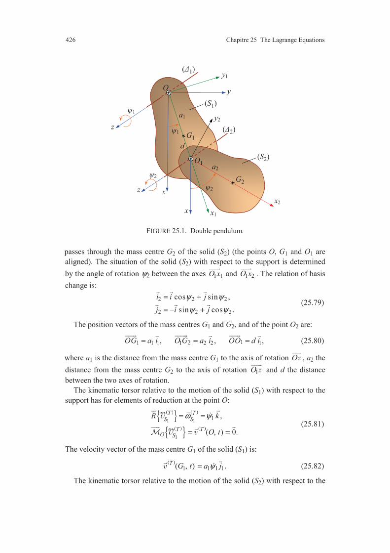
426 Chapitre 25 The Lagrange Equations
(S1)
(S2)
O
(1)
(2)
y
x
1
x
x2
y1
zy2
G1
G2
O1
d
a1
a2
1
2
x1
2 z
FIGURE 25.1. Double pendulum.
passes through the mass centre G2 of the solid (S2) (the points O, G1 and O1 are
aligned). The situation of the solid (S2) with respect to the support is determined
by the angle of rotation ψ2 between the axes 11O x
and 21O x
. The relation of basis
change is:
2 2 2
2 2 2
cos sin ,
sin cos .
i i j
j i j
ψ ψ
ψ ψ
= +
= − +
(25.79)
The position vectors of the mass centres G1 and G2, and of the point O2 are:
121 1 1 1 2 2 1, , ,OG a i O G a i OO d i= = =
(25.80)
where a1 is the distance from the mass centre G1 to the axis of rotation Oz
, a2 the
distance from the mass centre G2 to the axis of rotation 1O z
and d the distance
between the two axes of rotation.
The kinematic torsor relative to the motion of the solid (S1) with respect to the
support has for elements of reduction at the point O:
( ) ( )
( ) ( )
1 1
1
1 ,
( , ) 0.
T TS S
T TO S
R k
O t
ω ψ= =
= =
(25.81)
The velocity vector of the mass centre G1 of the solid (S1) is:
( )1 1 1 1( , )T G t a jψ=
. (25.82)
The kinematic torsor relative to the motion of the solid (S2) with respect to the

25.4 Applications 427
support has for elements of reduction at the point O1:
( ) ( )
( ) ( )
2 2
1 2
2
1 1 1
,
( , ) .
T TS S
T TO S
R k
O t d j
ω ψ
ψ
= =
= =
(25.83)
The velocity vector of the mass centre G2 of the solid (S2) is: ( ) ( ) ( )
122 1 1( , ) ( , )T T T
SG t O t O Gω= + ×
, (25.84)
hence: ( )
2 1 1 2 2 2( , )T G t d j a jψ ψ= + . (25.85)
25.4.3.3 Kinetic Energies
The calculation of the kinetic energies needs the determination of the kinetic
torsors, which introduce the masses and the operators of inertia of the solids. The
mass of the solid (S1) is denoted by m1 and its matrix of inertia at the point G1 in
the basis (1) = ( )1 1, , i j k
is:
( )
1
1 1 11
1 1 1 1
1 1 1
( )G
A F E
S F B D
E D C
− − = − − − −
I . (25.86)
Similarly, the mass of the solid (S2) is m2 and its matrix of inertia at the point G2
in the basis (2) = ( )2 2, , i j k
is:
( )
2
2 2 22
2 2 2 2
2 2 2
( )G
A F E
S F B D
E D C
− − = − − − −
I . (25.87)
Thus, it results that the kinetic torsor ( ) 1
TS relative to the motion of the solid
(S1) with respect to the support has for elements of reduction at the point G1:
( ) ( )
( ) ( ) ( )
1
1 11 1
1 1 1 1 1 1
1 1 1 1 1 1 1 1 1
( , ) ,
.
T TS
T TG GS S
R m G t m a j
S E i D j C k
ψ
ω ψ ψ ψ
= =
= = − − +
(25.88)
Similarly, the elements of reduction at the point G2 of the kinetic torsor relative
to the motion of the solid (S2) with respect to the support are:
( ) ( ) ( )( ) ( ) ( )
2
2 22 2
2 2 2 1 1 2 2 2
2 2 2 2 2 2 2 2 2
( , ) ,
.
T TS
T TG GS S
R m G t m d j a j
S E i D j C k
ψ ψ
ω ψ ψ ψ
= = +
= = − − +
(25.89)
The kinetic energy relative to the motion of the solid (S1) with respect to the
support is:
428 Chapitre 25 The Lagrange Equations
( ) ( ) ( ) 1 1
c 11
( )2
T T TS S
E S = ⋅ , (25.90)
with: ( ) ( ) ( ) 11 1 1
1T T T
O GS S SR G O= + ×
, (25.91)
or taking account of (25.88):
( ) ( )
1
21 1 1 1 1 1 1 1 1 1
TO S
E i D j C m a kψ ψ ψ= − − + +
. (25.92)
Introducing this result into Expression (25.90) leads to:
( ) ( )2 2c 1 1 1 1 1
1( )
2TE S C m a ψ= + . (25.93)
The kinetic energy relative to the motion of the solid (S2) with respect to the
support is:
( ) ( ) ( ) 2 2
c 21
( )2
T T TS S
E S = ⋅ , (25.94)
or expanding the product of the torsors at the point O1:
( ) ( ) ( ) ( ) ( ) 12 2
c 2 2 2 11 1
( ) ( , ) ( , )2 2
T T T T TOS S
E S m G t O t ω= +⋅ ⋅ , (25.95)
with: ( ) ( ) ( ) 1 22 2 2
12T T T
O GS S SR G O= + ×
. (25.96)
Taking account of (25.89), we obtain:
( ) ( )
1 22
2 2 2 2 2 2 2 2 2 2 1 2 1 2 2 2cos .
TO S
E i D j C m da m a kψ ψ ψ ψ ψ ψ ψ
=
− − + + − +
(25.97)
Introducing (25.83), (25.85) and (25.97) into Expression (25.95) for the kinetic
energy leads to:
( ) ( ) ( )2 2 2 2c 2 2 1 2 2 2 2 2 2 1 2 2 1
1 1( ) cos
2 2TE S m d C m a m daψ ψ ψ ψ ψ ψ= + + + − . (25.98)
From Expressions (25.93) and (25.98), we deduce that the kinetic energy of the
set (D) of the two solids is:
( )
( ) ( ) ( )c
2 2 2 2 21 1 1 2 1 2 2 2 2 2 2 1 2 2 1
( )1 1
cos .2 2
TE D
C m a m d C m a m daψ ψ ψ ψ ψ ψ
=
+ + + + + − (25.99)
25.4.3.4 Powers Developed
The mechanical actions exerted by the solid (S1) are: the action of gravity,
represented by the torsor ( ) 1e S ; the action of the support induced by the hinge
connection, represented by the torsor ( ) 1S ; the action of the solid (S2) induced
by the second hinge connection, represented by the torsor ( ) 2 1S . The power
25.4 Applications 429
developed by the action of gravity is:
( ) ( ) ( ) ( ) ( ) ( )
1 11 1 1e e eT T T
OS SP S S Sω= =⋅ ⋅
, (25.100)
with
( ) 1 1 1 1e sinO S m ga kψ= − . (25.101)
Hence: ( ) ( ) 1 1 1 1 1e sinTP S m gaψ ψ= − , (25.102)
and the power coefficients are:
( ) ( ) ( ) ( )
1 21 1 1 1 1e sin , e 0.T TP S m ga P Sψ ψψ= − = (25.103)
Similarly, the power developed by the action exerted by the support is:
( ) ( ) 1
1 1 1 1( ) ( )T TS
P S S N ψ= =⋅ , (25.104)
where N1 is the component along the direction k
of the moment at the point O of
the axis of the hinge connection. The power coefficients are:
( ) ( ) 1 21 1 1( ) , ( ) 0.T TP S N P Sψ ψ= = (25.105)
The power developed by the action of connection exerted by the solid (S2) is:
( ) ( ) 1
2 1 2 1 21 1 21 1( ) ( )T TS
P S S N dYψ ψ= = +⋅ , (25.106)
where N21 is the component along the direction k
of the moment at the point O1
and Y21 the component along the direction 1j
of the resultant of the action of con-
nection. The power coefficients are thus:
( ) ( ) 1 22 1 21 21 2 1( ) , ( ) 0.T TP S N dY P Sψ ψ= + = (25.107)
The mechanical actions exerted on the solid (S2) are reduced to the action of
gravity, represented by the torsor ( ) 2e S , and the action of the solid (S1)
induced by the hinge connection, represented by the torsor ( ) 1 2S opposed to
the torsor ( ) 2 1S . The power developed by the action of gravity is:
( ) ( ) ( ) ( )
22 2e eT T
SP S S= ⋅ , (25.108)
or expanding at the point O1:
( ) ( ) ( ) ( ) ( ) ( ) 122 2 1 2e e ( , ) eT T T
OSP S R S O t Sω= +⋅ ⋅
, (25.109)
with:
( ) 1 2 2 2 2e sinO S m ga kψ= − . (25.110)
Thus: ( ) ( ) 2 2 1 1 2 2 2 2e sin sinTP S m gd m gaψ ψ ψ ψ= − − . (25.111)
The power coefficients are:

430 Chapitre 25 The Lagrange Equations
( ) ( ) ( ) ( )
1 22 2 1 2 2 2 2e sin , e sin .T TP S m gd P S m gaψ ψψ ψ= − = − (25.112)
The expression of the power developed by the action of connection exerted by the
solid (S1) on the solid (S2) has the same form as Expression (25.109). By applying
this expression to the action of connection, we obtain:
( ) 1 2 21 1 21 2( )TP S dY Nψ ψ= − − , (25.113)
hence the power coefficients:
( ) ( ) 1 21 2 21 1 2 21( ) , ( ) .T TP S dY P S Nψ ψ= − = − (25.114)
25.4.3.5 Lagrange Equations
The Lagrange equations for the set (D), constituted of the two solids, are
written from (25.39) as:
( )( ) ( )( ) ( ) ( ) ( ) ( ) ( ) ( ) ( ) ( ) ( ) ( )
c c 1 1 2 1
2 1 2
1 2
de
d
e ,
, 115(25. ).
i i i
i i
T T T T Tq q q
i iT T
q q
i
E D E D P S P S P St q q
P S P S
q ψ ψ
∂ ∂− = + +
∂ ∂
+ +
=
1. Lagrange Equation relative to the parameter ψ1
We have:
( )( ) ( ) ( )2 2c 1 1 1 2 1 2 2 2 2 1
1
cosTE D C m a m d m daψ ψ ψ ψψ∂
= + + + −∂
, (25.116)
( )( ) ( ) ( )
( ) ( )
2 2c 1 1 1 2 1 2 2 2 2 1
1
2 2 2 2 1 2 1
dcos
dsin ,
TE D C m a m d m dat
m da
ψ ψ ψ ψψ
ψ ψ ψ ψ ψ
∂= + + + −
∂− − −
(25.117)
( )( ) ( )c 2 2 1 2 2 11
sin .TE D m da ψ ψ ψ ψψ∂
= −∂
(25.118)
Hence the first Lagrange equation:
( ) ( ) ( )
( )
2 2 21 1 1 2 1 2 2 2 2 1 2 2 1
1 1 2 1 1 21
cos sin
sin .
C m a m d m da
m a m d g N N
ψ ψ ψ ψ ψ ψ ψ
ψ
+ + + − − −
= − + + +
(25.119)
2. Lagrange Equation relative to the parameter ψ2
We have:
( )( ) ( ) ( )2c 2 2 2 2 2 2 1 2 1
2
cosTE D C m a m daψ ψ ψ ψψ∂
= + + −∂
, (25.120)
( )( ) ( ) ( )
( ) ( )
2c 2 2 2 2 2 2 1 2 1
2
2 2 1 2 1 2 1
dcos
dsin ,
TE D C m a m dat
m da
ψ ψ ψ ψψ
ψ ψ ψ ψ ψ
∂= + + −
∂− − −
(25.121)

A.25 Appendix 431
( )( ) ( )c 2 2 1 2 2 12
sin .TE D m da ψ ψ ψ ψψ∂
= − −∂
(25.122)
Hence the second Lagrange equation:
( ) ( ) ( )2 22 2 2 2 2 2 1 2 1 1 2 1
2 2 1 21
cos sin
sin .
C m a m da
m ga N
ψ ψ ψ ψ ψ ψ ψ
ψ
+ + − + −
= − −
(25.123)
The two equations (25.119) and (25.123) constitute the two equations of the
motions of the double pendulum.
A.25 APPENDIX
A.25.1 Properties of Derivatives of Rotation Vector
The instantaneous vector of rotation relative to the motion of the solid (S) with
respect to the reference (T) is written (9.12):
( ) 3
TS Sk i kω ψ θ ϕ= + +
. (A.25.1)
The expressions in the bases ( ), , i j k
and ( ), , S S Si j k
are given respectively by
Expressions (9.16) and (9.17).
The relations between the different bases, introduced by the rotations, are
expressed by Relations (9.13) to (9.15). Thus:
— Rotation of angle ψ about the direction k
:
3 3 3
3 3 3
cos sin , cos sin ,
sin cos , sin cos ,
. .
i i j i i j
j i j j i j
k k
ψ ψ ψ ψ
ψ ψ ψ ψ
= + = −
= − + = +
(A.25.2)
— Rotation of angle θ about the direction 3i
:
3 3
4 3 3 4
3 4
, ,
cos sin , cos sin ,
sin cos . sin cos .
S
S S
i i
j j k j j k
k j k k j k
θ θ θ θ
θ θ θ θ
= + = − = − + = +
(A.25.3)
— Rotation of angle ϕ about the direction Sk
:
3 4 3
3 4 4
cos sin , cos sin ,
sin cos , sin cos ,
. .
S S S
S S S
S S
i i j i i j
j i j j i j
k k
ϕ ϕ ϕ ϕ
ϕ ϕ ϕ ϕ
= + = −
= − + = +
(A.25.4)
These basic relations allow us to express the derivatives in the reference (T)
with respect to time of the vectors k
, 3i
and Sk
. The vector k
being independent

432 Chapitre 25 The Lagrange Equations
of time in the reference (T), we have:
( )d
0d
T
kt
=
. (A.25.5)
The derivative of the vector 3i
is obtained by writing:
( )
( )3 3 4d
cos sind
T
Si j j kt
ψ ψ θ θ= = −
. (A.25.6)
In the basis ( ), , S S Si j k
its expression is thus:
( )
3d
cos sin cos cos sind
T
S S Si i j kt
ψ θ ϕ ψ θ ϕ ψ θ= + −
. (A.25.7)
From (A.25.3), the derivative of Sk
is written:
( ) ( )
3 3d d
sin cos sind d
T T
Sk j j kt t
θ θ θ θ θ= − − −
, (A.25.8)
or
( )
3 3d
sin cos sind
T
Sk i j kt
ψ θ θ θ θ θ= − − −
. (A.25.9)
Transforming the vectors 3i
, 3j
and k
in the basis ( ), , S S Si j k
, we obtain finally:
( )
( ) ( )dsin cos sin sin cos cos
d
T
S S Sk i jt
ψ θ ϕ θ ϕ ψ θ ϕ θ ϕ= − + − −
. (A.25.10)
From Expression (9.17) of the rotation vector in the basis ( ), , S S Si j k
, we
deduce easily the following relations:
( )( )
0,S
TSω
ψ∂
=∂
(A.25.11)
( )( )
sin cos cos cos sin ,S
TS S S Si j kω ψ ϕ θ ψ ϕ θ ψ θ
θ∂
= + −∂
(A.25.12)
( )( ) ( ) ( )sin cos sin sin sin cos .
ST
S S Si jω θ ϕ ψ ϕ θ ψ ϕ θ θ ϕϕ
∂= − − + − −
∂
(A.25.13)
The comparison of Relations (A.25.5) and (A.25.11), (A25.7) and (A.25.12), then
(A.25.10) and (A.25.13) leads to the relations:
( ) ( )( )
( ) ( )( )
( ) ( )( )
3d d d
, , .d d d
T S T S T ST T T
S S S Sk i kt t t
ω ω ωψ θ ϕ
∂ ∂ ∂= = =
∂ ∂ ∂
(A.25.14)
From Relation (A.25.1), we deduce:
( )( )
ST
S kωψ
∂=
∂
. (A.25.15)

A.25 Appendix 433
Deriving this result with respect to time, we obtain then:
( ) ( )( )
( ) ( )( )d d
d d
T S T ST T
S Skt t
ω ωψ ψ
∂ ∂= =
∂ ∂
. (A.25.16)
While operating in the same way with the variables θ and ϕ , we obtain:
( ) ( )( )
( )( )d
d
T S ST T
S St
ω ωθθ
∂ ∂=
∂∂
, (A.25.17)
( ) ( )( )
( )( )d
d
T S ST T
S St
ω ωϕ ϕ
∂ ∂=
∂ ∂
. (A.25.18)
These three relations can be written in the form:
( ) ( )( )
( )( )d
, , , d
T S ST T
S S iii
Qt QQ
ω ω ψ θ ϕ∂ ∂= =
∂∂
. (A.25.19)
A.25.2 Properties of the Derivatives of the Velocity Vector of the Mass Centre
In the case where the position of the mass centre is defined by the parameters
of translation pi, the velocity vector is expressed as:
( )( ) ( )
1
d( , ) , 3.
d
kT TT
jj
j
G t OG p OG kt p
=
∂= = ≤
∂
(A.25.20)
From this expression, we deduce:
— first:
( )( )
( )2
1
( , ) ,
kT TT
ji i j
j
G t p OGp p p
=
∂ ∂=
∂ ∂ ∂
(A.25.21)
— then: ( )
( )( )
( , ) .T T
T
i i
G t OGp p
∂ ∂=
∂ ∂
(A.25.22)
Thus we obtain:
( ) ( )( )
( )2
1
d( , ) ,
d
kT T TT
ji i j
j
G t p OGt p p p
=
∂ ∂=
∂ ∂ ∂
(A.25.23)
The comparison of Expression (A.25.21) and (A.25.23) leads to the relation:
( ) ( )( )
( )( )
d
( , ) ( , )d
T T TT T
i i
G t G tt p p
∂ ∂=
∂ ∂
. (A.25.24)
434 Chapitre 25 The Lagrange Equations
EXERCISES
25.1 Using Lagrange equations, derive the equations of motion of the set of the
two solids considered in Exercise 24.1.
25.2 Similarly, derive the equations of motion of the radar antenna studied in
Exercise 24.2.
COMMENTS
The Lagrange equations constitute an efficient tool to obtain the equa-
tions of motion directly. Establishing these equations is rather complex and
the reader will endeavour first to understand the development which leads
to these equations.
The Lagrange equations which constitute the equations of motion are
Equations (25.30) in the case of one body and Equations (25.39) for a set
of bodies. The reader will have to thus know these equations, as well as the
way for applying the equations. The examples given at the end of the
chapter illustrate well the way for using the Lagrange equations. The reader
will apply them to the cases considered in the two exercises.

Part VI
Numerical Methods for Solving Differential Equations.
Application to Equations of Motion
The equations of motion of bodies are generally complex, and the
most of the equations cannot be solved analytically. This part is an
introduction to the numerical resolution of the equations of motion.
The tools which will be introduced can be easily implemented using a
software of general use, such as Matlab.


CHAPTER 26
Numerical Methods for Solving First Order Differential Equations
26.1 GENERAL ELEMENTS
26.1.1 Problem with Given Initial Conditions
A differential equation of the first order can be put in the general form:
d
( , ) or ( , )d
yf t y y f t y
t= = . (26.1)
The problem consists in searching for the function y of the variable t, of which the
derivative with respect to this variable is known. The variable t can be arbitrary.
When we shall apply the results obtained to the resolution of the equations of
motion, the variable t will be the time variable.
In a general way, there exists an infinity of solutions to Equation (26.1), differ-
ring by an arbitrary constant. Setting a value 0y of the solution for an initial value
t0 of the variable t: 0 0( ),y y t= the solution is then unique. The problem is said to
be a problem with given initial conditions. We shall limit thereafter the analysis to
this type of problem, which makes it possible to solve the equations of motion.
The problem with given initial conditions is thus stated in the following way:
Find the function y(t), defined on the interval [ ]0 f, t t , satisfying:
0 0d
( , ) with ( ) .d
yf t y y t y
t= = (26.2)
It is shown that this problem admits a unique solution if the function f satisfies
the Lipschitz condition:
1 2 1 2 ( , ) ( , ) f t y f t y L y y− ≤ − , (26.3)
where L is a positive constant. It is also shown that if the derivative of the
function f with respect to y is continuous and bounded, then f satisfies the
Lipschitz condition .

438 Chapter 26 Numerical Methods for Solving First Order Differential Equations
TABLE 26.1 Numerical values and exact values.
variable t 0t 1 0t t h= + 2 0 2t t h= + .... 0it t ih= + .... 0nt t nh= +
computed values for y 0y 1y 2y .... iy .... ny
exact values for y 0( )y t 1( )y t 2( )y t .... ( )iy t .... ( )ny t
26.1.2 General Method of Resolution
The general method of numerical resolution consists in increasing the variable
t, from the initial value t0, by steps equal to h ( )h t= ∆ and calculating succes-
sively the values of the function y, for 1 0 ,t t h= + 2 0 2 ,t t h= + ..., 0 ,it t ih= + ...,
fnt t= . The computed values will be denoted by yi and the exact values by y(ti)
(Table 26.1). The numerical procedure used must lead to 0( ).iy y t ih≈ + It will be
possible to use either a constant step independent of the variable t (h = cst), or a
variable step function of the variable t (h = h(t)). The use of a variable step will
make it possible to control the value of the step according to the value of the
variable t.
The numerical procedures can be divided into single-step procedures and
multiple-step procedures. In the single-step procedures, each computed value 1iy +
is only deduced as a function of the step and of the preceding value yi. At each
stage of the procedure, calculations are independent of the preceding stages, hence
the name of single-step procedures. These methods are easily implemented and
their interest lies in the possibility of easily using variable step in the course of the
computation. In contrast, the multiple-step procedures re-use former calculations:
the value of 1iy + is evaluated from the preceding values yi , 1iy − , ..., y1, y0. Such
methods make it possible to increase the speed of calculations clearly. However,
the use of a variable step in the course of computation raises difficulties.
A large variety of numerical methods was developed to solve the initial value
problems (26.2). Most of the procedures were generalized so as to be able to apply
to higher order problems. This chapter aims to present some elements on these
methods of numerical resolution, with for objective to apply the results to the
numerical resolution of the equations of motion.
26.1.3 Euler Method
The Euler method is practically not used owing to the fact that it is too slow to
reach accurate values. However, its simplicity constitutes a good introduction to
the other more powerful methods. The Euler method consists in deriving the value
of 1iy + starting from the value yi and considering only the first order term of the
Taylor series:
( ) ( ) ( )i i iy t h y t hy t+ = + . (26.4)

26.1 General Elements 439
t1 t0 t2 t3 t5 t4 t7 t6 t8 t
y
h
numerical values
exact values
FIGURE 26.1. Approximation using theEuler method.
The set of the values of the function is thus derived from the relation:
1 ( , ), 0, 1, . . . , .i i i iy y h f t y i n+ = + = (26.5)
A difference equation is then substituted for the differential equation (26.2). Thus,
the curve y(t) is replaced by its tangent at each step of the procedure (Figure 26.1).
As an example, we consider the differential equation:
1/3y t y= , (26.6)
with for initial condition (1) 1y = . This differential equation has an exact solution:
3/22 2
3
ty
+=
. (26.7)
Table 26.2 compares the results obtained by the Euler method for different values
of the step with the exact values (26.7) of the function. The values reported in
TABLE 26.2 Results derived from the Euler method.
variable t 1 2 3 4 5
exacty 1.0000 2.8284 7.0211 14.6969 27.0000
0.10h = iy 1.0000 2.7239 6.7148 14.0799 25.9595
error 0.0000 –0.1045 –0.3064 –0.6171 –1.0405
0.05h = iy 1.0000 2.7754 6.8662 14.3856 26.4759
error 0.0000 –0.0530 –0.1549 –0.3113 –0.5241
0.01h = iy 1.0000 2.8177 6.9899 14.6342 26.8946
error 0.0000 –0.0107 –0.0313 –0.0627 –0.1054
440 Chapter 26 Numerical Methods for Solving First Order Differential Equations
the table show an appreciable improvement of the numerical values when the step
decreases, at the price of an important increase of the computing delay. For
example the 25.9595 value for t = 5 is obtained using 50 steps for computation,
whereas the 26.8946 value needed 500 steps.
26.2 SINGLE-STEP METHODS
26.2.1 General Elements
26.2.1.1 Formulation
The single-step methods replace the function ( , )i if t y of the Euler method by a
more general function ( , , )i it y hϕ . The evaluation of 1iy + at a given stage is
derived from the relation:
1 ( , , )i i i iy y h t y hϕ+ = + . (26.8)
The differential equation (26.2) is replaced by a non-linear difference equation.
The choice of the function depends on the method used. Thus, the Euler method is
a single-step method, for which the function ϕ is reduced to the function f.
26.2.1.2 Convergence
The methods used must lead to a decrease in the error when the step of compu-
tation decreases, the error having to vanish when the step becomes infinitely
small. It is said that the method must be convergent.
The numerical procedure is convergent on the interval [ ]0 f, t t if, for all the
values yi calculated, the maximum difference with the exact solution decreases
when the step h of computation decreases.
Thus the method is convergent if:
0max ( ) 0, when 0i i
i ny y t h
≤ ≤− → → . (26.9)
26.2.1.3 Stability
Furthermore, the errors induced by the method should not be amplified. It is
said that the method must be stable.
A method is said to be stable if a perturbation on the computed value of yi
involves only a small perturbation on the value of 1iy + , and that whatever the step
value h.
An unstable procedure leads to an amplification of the errors at each step of

26.2 Single-Step Methods 441
computation. It is shown that if the function ϕ satisfies the Lipschitz condition:
( , , ) ( , , ) , 0i i i i i it y y h t y h L y Lϕ ϕ+ ∆ − ≤ ∆ < < ∞ , (26.10)
then the method is stable.
26.2.1.4 Consistence
The method of approximation (26.8) is consistent with the differential equation
if:
( )
10 0
1lim max ( , , ) 0i i i ih i n
y y t y hh
ϕ+→ ≤ ≤
− − →
. (26.11)
Consistency means that the approximation (26.8) must be a probable and well
constructed approximation. It is shown that the method is consistent if:
( , , 0) ( , )t y f t yϕ = . (26.12)
If the method is stable and consistent, then it is convergent for any value of the
initial value.
26.2.1.5 Order
A numerical method is said to be convergent of order p, if:
0max ( ) , 0p
i ii n
y y t Kh K≤ ≤
− ≤ < < ∞ . (26.13)
We observe that if the step is divided by the value λ, the error on the approxi-mation is divided by pλ . Hence the interest to have a high order method.
26.2.1.6 Example of the Euler Method
We considered that the Euler method is a single-step method, for which fϕ = .
1. The method is consistent if ( , , 0) ( , )i i i it y f t yϕ = . This result is immediate, since fϕ = does not depend on the step h. The Euler method is thus consistent.
2. The method is stable if the Lipschitz condition (26.10) on the function ϕ is satisfied. The Euler method is stable since fϕ = , and that the function f by as-sumption satisfies the Lipschitz condition (26.3). The Euler method is thus con-vergent.
3. It is possible to show (the demonstration is not immediate) that:
( ) , 1, 2, . . . , .i iy y t Kh i n− = = (26.14)
The Euler method is thus locally (for each step) of order 1. The local error (26.14)
is induced to each stage of the procedure between the step i and the step 1i + .
These errors are propagated through the stages of the procedure and it is generally
not possible to have a precise idea, a priori, of the propagation of the errors. The
results of Table 26.1 show that the order 1 of the Euler method is maintained, in
the example considered, throughout the stages going from 0 1t = to f 5t = .

442 Chapter 26 Numerical Methods for Solving First Order Differential Equations
26.2.2 Methods of Runge-Kutta Type
26.2.2.1 General Formulation
In the methods of Runge-Kutta type, the function ( , )t yϕ of the approximation
relation (26.8) is formed as a linear combination of the values of the function
( , )f t y calculated at suitable points ( , )j jt y , in such a way to obtain high order
procedures. The Runge-Kutta methods lead to errors clearly lower than that
obtained by the Euler method, when the implementation remains simple. In these
methods, the approximation 1iy + is expressed as a function of the approximation
iy in the form (26.8), with:
1 1 2 2( , , ) . . . i i n nt y h k k kϕ ϕ ϕ ϕ= + + + , (26.15)
where 1 2, , . . . , nk k k are coefficients and 1 2, , . . . , nϕ ϕ ϕ are the values of the
function ( , )f t y expressed as:
1
2 1 1 1
3 2 2 2
1 1 1
( , ) ,
( , ) ,
( , ) ,
.
.
.
( , ) .
i i
i i
i i
n i n i n n
f t y
f t a h y
f t a h y
f t a h y
ϕ
ϕ α ϕ
ϕ α ϕ
ϕ α ϕ− − −
=
= + +
= + +
= + +
(26.16)
26.2.2.2 Runge-Kutta Methods of Order 2
In the case of the Runge-Kutta methods of order 2, the function (26.15) is
expressed in the form:
1 1 2 2( , , )i it y h k kϕ ϕ ϕ= + , (26.17)
with
1
2 1
( , ) ,
( , ) .
i i
i i
f t y
f t ah y
ϕ
ϕ αϕ
=
= + + (26.18)
The coefficients k1, k2, a and α are derived from the Taylor expansion to the
second order of the function y at the vicinity of ti. Thus:
2
( ) ( ) ( ) ( )2
i i i ih
y t h y t hy t y t+ = + + , (26.19)
with
( ) ( , )i i iy t f t y= , (26.20)
and
d d
d d
f f f y fy f y
t t y t y
∂ ∂ ∂= = + = +
∂ ∂ ∂ . (26.21)
26.2 Single-Step Methods 443
Thus:
( ) ( , ) ( , ) ( , )i i i i i i if
y t f t y t y f t yy
∂= +
∂ . (26.22)
The expansion (26.19) is thus written:
2
( ) ( ) ( , ) ( , ) ( , ) ( , )2
i i i i i i i i i ifh
y t h y t h f t y f t y t y f t yy
∂ + = + + + ∂ . (26.23)
Moreover, the function 2ϕ (26.18) expanded to the first order at the vicinity of
( , )i it y is written as:
1 1( , ) ( , ) ( , ) ( , )i i i i i i i if
f t ah y f t y ah f t y t yy
αϕ αϕ∂
+ + = + +∂
, (26.24)
or
1( , ) ( , ) ( , ) ( , ) ( , )i i i i i i i i i if
f t ah y f t y ah f t y h f t y t yy
αϕ α∂
+ + = + +∂
. (26.25)
The evaluation of 1iy + at a given stage is thus written finally, from (26.8), (26.17),
(26.18) and (26.25), in the form:
( ) 2
1 1 2 2( , ) ( , ) ( , ) ( , )i i i i i i i i i if
y y k k h f t y h k f t y t y a f t yy
α+∂ = + + + + ∂
. (26.26)
Comparison between Expressions (26.23) and (26.26) leads to the relations:
1 2
12 2
12 2
1,
,
.
k k
k
ak
α
+ =
=
=
(26.27)
Hence the expressions of the parameters:
1
2
,
2 1,
2
1.
2
a
ak
a
ka
α =
−=
=
(26.28)
The choice of the value of the parameter a is arbitrary, and this choice determines
the method used.
1. In the case where we choose 1/2a α= = , the values of the parameters k1 and
k2 are: 1 0k = and 2 1k = . These values lead to the improved Euler method, where
the evaluation of 1iy + is computed in the form:
1 1( , )2 2
i i i ih h
y y h f t y ϕ+ = + + + , (26.29)
with:
1 ( , )i if t yϕ = . (26.30)

444 Chapter 26 Numerical Methods for Solving First Order Differential Equations
2. In the case where we choose 1a α= = , the values of the parameters k1 and
k2 are 1 2 1/2k k= = . These values lead to the method known as Euler-Cauchy,
where the evaluation of 1iy + is computed in the form:
( )1 1 22
i ih
y y ϕ ϕ+ = + + , (26.31)
with:
1
2 1
( , ) ,
( , ) .
i i
i i
f t y
f t h y h
ϕ
ϕ ϕ
=
= + + (26.32)
The Euler-Cauchy method can be considered as the cumulative result of the
Euler method applied to the two half-intervals [ ], /2i it t h+ and [ ]/2, i it h t h+ + .
Indeed, the approximation (26.5) is written for these two intervals:
12
( , )2
i i ii
hy y f t y
+= + , (26.33)
1 1 12 2 2
1 ( , )2
i i i i
hy y f t y+ + + +
= + . (26.34)
Combination of these two results leads well to Relation (26.31).
The improved Euler and Euler-Cauchy methods are methods of order 2. Table
26.3 reports the results derived from the Euler-Cauchy method to solve Equation
(26.6). The results show that the method is effectively of order 2. In the case
where the step is equal to 0.01, the maximum error observed is equal to 48 10−− × .
26.2.2.3 Runge-Kutta Methods of Order 4
In the case of the Runge-Kutta methods of order 4, the function (26.15) is
expressed in the form:
1 1 2 2 3 3 4 4( , , )i it y h k k k kϕ ϕ ϕ ϕ ϕ= + + + , (26.35)
TABLE 26.3 Results derived from the Euler-Cauchy method.
variable t 1 2 3 4 5
exacty 1.000000 2.828427 7.021132 14.696938 27.000000
0.10h = iy 1.000000 2.827609 7.018633 14.692080 26.992260
error 0.000000 –0.000818 –0.002499 –0.004859 –0.007740
0.05h = iy 1.000000 2.828219 7.020495 14.695701 26.998031
error 0.000000 –0.000208 –0.000637 –0.001237 –0.001969
0.01h = iy 1.000000 2.828419 7.021106 14.696889 26.999920
error 0.000000 –0.000008 –0.000026 –0.000050 –0.000080
26.2 Single-Step Methods 445
with
1
2 1 1 1
3 2 2 2
4 3 3 3
( , ) ,
( , ) ,
( , ) ,
( , ) .
i i
i i
i i
i i
f t y
f t a h y
f t a h y
f t a h y
ϕ
ϕ α ϕ
ϕ α ϕ
ϕ α ϕ
=
= + +
= + +
= + +
(26.36)
The various coefficients intervening in the functions (26.35) and (26.36) are
derived by a method comparable to that used in the preceding subsection, by
expanding to the forth order in Taylor series the function y at the vicinity of ti(Exercise 26.1). The identification of the expansions leads at first to the equality
of the coefficients αi and ai:
, 1, 2, 3.i ia iα = = (26.37)
Then to the equations:
11 2 3 4 3 1 2 4 2 3 6
2 21 12 1 3 2 4 3 3 1 2 4 2 32 8
2 2 2 2 21 12 1 3 2 4 3 3 1 2 4 2 33 12
3 3 3 1 12 1 3 2 4 3 4 1 2 34 24
1, ,
, ,
, ,
, .
k k k k k a a k a a
k a k a k a k a a k a a
k a k a k a k a a k a a
k a k a k a k a a a
+ + + = + =
+ + = + =
+ + = + =
+ + = =
(26.38)
The system of these equations is overdetermined: eight equations for seven un-
knowns. The usual solution which is considered is:
1 1 11 2 3 1 4 2 32 6 3
, 1, , .a a a k k k k= = = = = = = (26.39)
The evaluation of 1iy + at the step i is thus computed in the form:
( )1 1 2 3 42 26
i ih
y y ϕ ϕ ϕ ϕ+ = + + + + , (26.40)
with
1
12
23
4 3
( , ) ,
( , ) ,2 2
( , ) ,2 2
( , ) .
i i
i i
i i
i i
f t y
hf t y
hf t y
f t h y
ϕ
ϕϕ
ϕϕ
ϕ ϕ
=
= + +
= + +
= + +
(26.41)
Table 26.3 reports the results obtained by this Runge-Kutta method to solve the
differential equation (26.6). These results show that this method is effectively of
order 4, making it possible to decrease clearly the number of values to compute.
The interest of this method lies thus in a high precision associated with a rather
simple implementation.
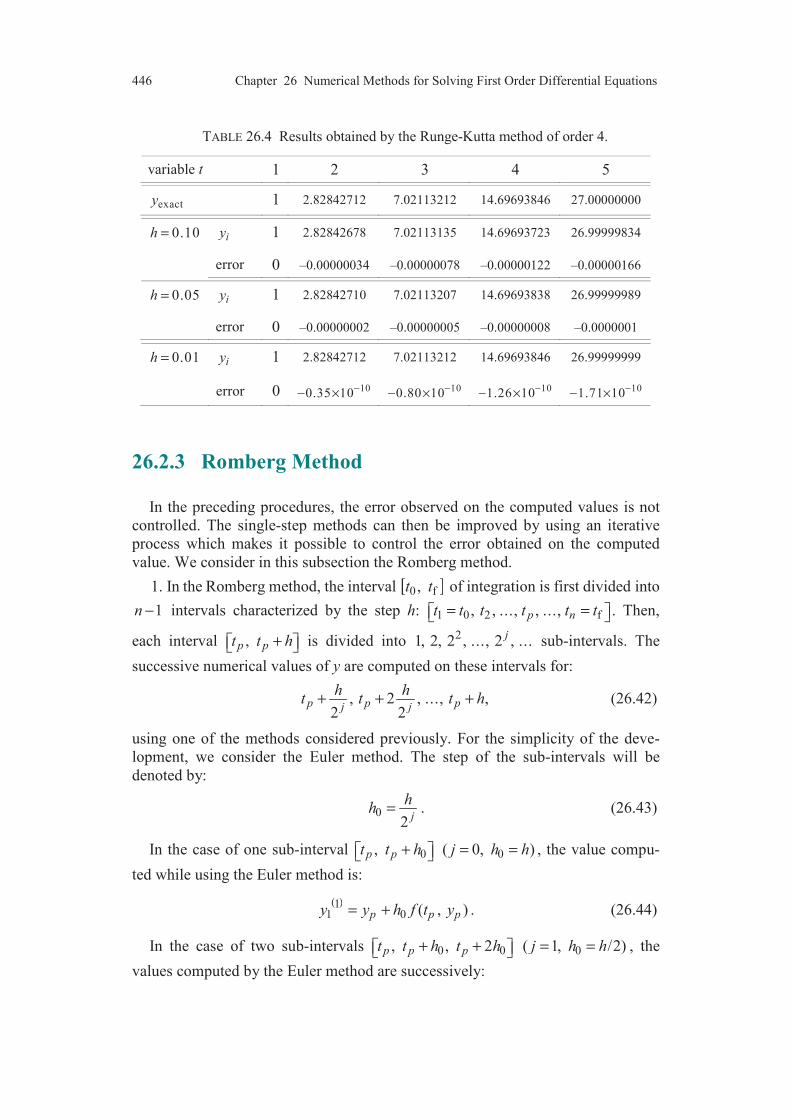
446 Chapter 26 Numerical Methods for Solving First Order Differential Equations
TABLE 26.4 Results obtained by the Runge-Kutta method of order 4.
variable t 1 2 3 4 5
exacty 1 2.82842712 7.02113212 14.69693846 27.00000000
0.10h = iy 1 2.82842678 7.02113135 14.69693723 26.99999834
error 0 –0.00000034 –0.00000078 –0.00000122 –0.00000166
0.05h = iy 1 2.82842710 7.02113207 14.69693838 26.99999989
error 0 –0.00000002 –0.00000005 –0.00000008 –0.0000001
0.01h = iy 1 2.82842712 7.02113212 14.69693846 26.99999999
error 0 100.35 10−− × 100.80 10−− × 101.26 10−− × 101.71 10−− ×
26.2.3 Romberg Method
In the preceding procedures, the error observed on the computed values is not
controlled. The single-step methods can then be improved by using an iterative
process which makes it possible to control the error obtained on the computed
value. We consider in this subsection the Romberg method.
1. In the Romberg method, the interval [ ]0 f, t t of integration is first divided into
1n − intervals characterized by the step h: 1 0 2 f, , ..., , ...,p nt t t t t t= = . Then,
each interval , p pt t h+ is divided into 21, 2, 2 , ..., 2 , ...j sub-intervals. The
successive numerical values of y are computed on these intervals for:
, 2 , ..., ,2 2
p p pj j
h ht t t h+ + + (26.42)
using one of the methods considered previously. For the simplicity of the deve-
lopment, we consider the Euler method. The step of the sub-intervals will be
denoted by:
02 j
hh = . (26.43)
In the case of one sub-interval 0, p pt t h+ 0( 0, )j h h= = , the value compu-
ted while using the Euler method is:
( )11 0 ( , )p p py y h f t y= + . (26.44)
In the case of two sub-intervals 0 0, , 2p p pt t h t h+ + 0( 1, /2)j h h= = , the
values computed by the Euler method are successively:
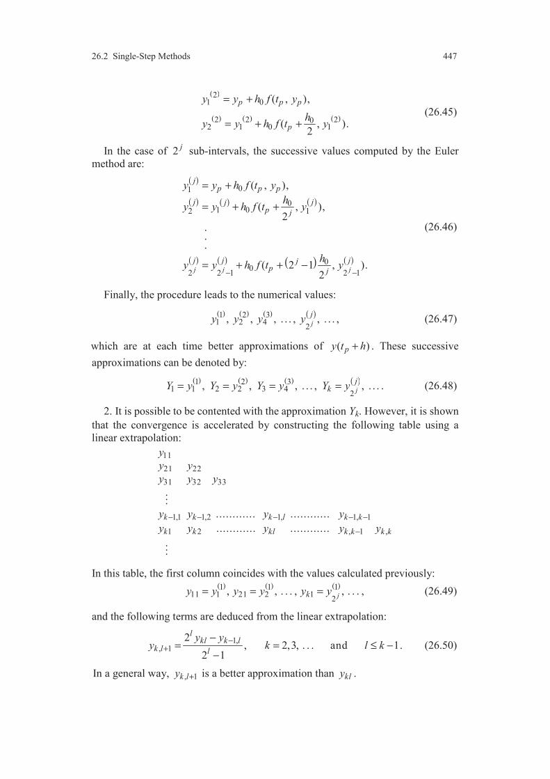
26.2 Single-Step Methods 447
( )
( ) ( ) ( )
21 0
2 2 202 1 0 1
( , ),
( , ).2
p p p
p
y y h f t y
hy y h f t y
= +
= + + (26.45)
In the case of 2 j sub-intervals, the successive values computed by the Euler
method are:
( )
( ) ( ) ( )
( ) ( ) ( ) ( )
01
01 02 1
00
2 2 1 2 1
( , ),
( , ),2
.
.
.
( 2 1 , ).2
j j j
jp p p
j jjp j
j j jjp j
y y h f t y
hy y h f t y
hy y h f t y
− −
= +
= + +
= + + −
(26.46)
Finally, the procedure leads to the numerical values:
( ) ( ) ( ) ( )
1 2 31 2 4
2, , , . . . , , . . . ,j
jy y y y (26.47)
which are at each time better approximations of ( )py t h+ . These successive
approximations can be denoted by:
( ) ( ) ( ) ( )
1 2 31 1 2 2 3 4
2, , , . . . , , . . . .j
jkY y Y y Y y Y y= = = = (26.48)
2. It is possible to be contented with the approximation Yk. However, it is shown
that the convergence is accelerated by constructing the following table using a
linear extrapolation:
11
21 22
31 32 33
1,1 1,2 1, 1, 1
1 2 , 1 ,
. ..
............ ............
............ ............
. ..
k k k l k k
k k kl k k k k
y
y y
y y y
y y y y
y y y y y− − − − −
−
In this table, the first column coincides with the values calculated previously: ( ) ( ) ( )
1 1 1
11 1 21 2 12
, , . . . , , . . . ,jky y y y y y= = = (26.49)
and the following terms are deduced from the linear extrapolation:
1,
, 1
2, 2,3, . . . and 1.
2 1
lkl k l
k l l
y yy k l k
−+
−= = ≤ −
− (26.50)
In a general way, , 1k ly + is a better approximation than kly .

448 Chapter 26 Numerical Methods for Solving First Order Differential Equations
11y
21y 22y 22y
32y 33y
11y
21y
31y
21y
31y 32y
11y
22y
31y
41y 42y
11y
21y
33y
22y
32y
The table is constructed gradually starting from the values computed by the Euler
method: y11, y21, ..., yk1, ..., in the following way:
In the process of forming the table, we observe that we need to keep only one row
to derive the following row. This remark implies that it is not necessary to store
the 2-dimension table ykl, but simply a 1-dimension table Tk, by using the follo-
wing process for filling the table:
In forming the table, we have thus:
1k l klT y− + = , (26.51)
and Relation (26.50) is written:
12
, 2, 3, . . . , 1,2 1
lk l k l
k l l
T TT k l k− + −
−−
= = = −−
(26.52)
with for 1 111, k T y= = . (26.53)
The procedure of computation is stopped when the difference between the last
computed value k lT − and the preceding one 1k lT − + is lower in absolute value than
the desired precision. The value computed at the step p + 1 is then k lT − . Thus:
1p k ly T+ −= (26.54)
Table 26.5 reports the results obtained by the Euler-Romberg method for
solving the differential equation (26.6). The main step chosen is equal to 1: the
interval [1, 5] of integration is thus divided into 4 intervals only. The results
obtained are reported with two imposed values of precision: the one higher than
1T
2T 1T 1T
2T 1T
1T
2T
3T
2T
3T 2T
1T
1T
3T
4T 3T
1T2T
1T
2T 1T

26.3 Multiple-Step Methods 449
TABLE 26.5 Results derived from the Euler-Romberg method.
variable t 1 2 3 4 5
yexact 1 2.82842712 7.02113212 14.69693846 27.00000000
desired precision higher than 0.01
yp 1 2.8277 7.0194 14.6946 26.9971
error 048 10−− × 31.7 10−− × 32.3 10−− × 32.9 10−− ×
number of
iterations0 3 3 4 4
desired precision higher than 10–5
yp 1 2.82842723 7.02113238 14.69693900 27.00000081
error 071.08 10−× 72.6 10−× 75.4 10−× 78.1 10−×
number of
iterations0 5 5 5 5
0.01 and the other higher than 10–5. The number of iterations necessary at each
step to reach the desired precision is also reported in the table.
26.3 MULTIPLE-STEP METHODS
26.3.1 Introduction to the Multiple-Step Methods
In the single-step methods, the numerical computations are independent of the
computations for the preceding steps. The multiple-step methods consist in re-
using the numerical values computed in the preceding steps, thus allowing to
improve the speed of the computations.
The solution y(t) of the differential equation satisfies the relation:
[ ]0 f( ) ( ) ( , ( )) d , , ,t t
t
y t t y t f u y u u t t t t t+∆
+ ∆ = + ∀ + ∆ ∈ . (26.55)
If yp are the computed values of the solution at the point tp, we can substitute for
the function ( )f t an interpolation polynomial P(t), taking at the point tp the values
( , )p p pf f t y= . On replacing the integral of f by the integral of the polynomial P,
we shall obtain then an approximation of ( ) ( )y t t y t+ ∆ − .
If we are at the step 1 ( 0, 1, . . .)i i+ = corresponding to the value ti of the
variable t, we know the approximations 1 2, , , . . . ,i i iy y y− − evaluated at the prece-
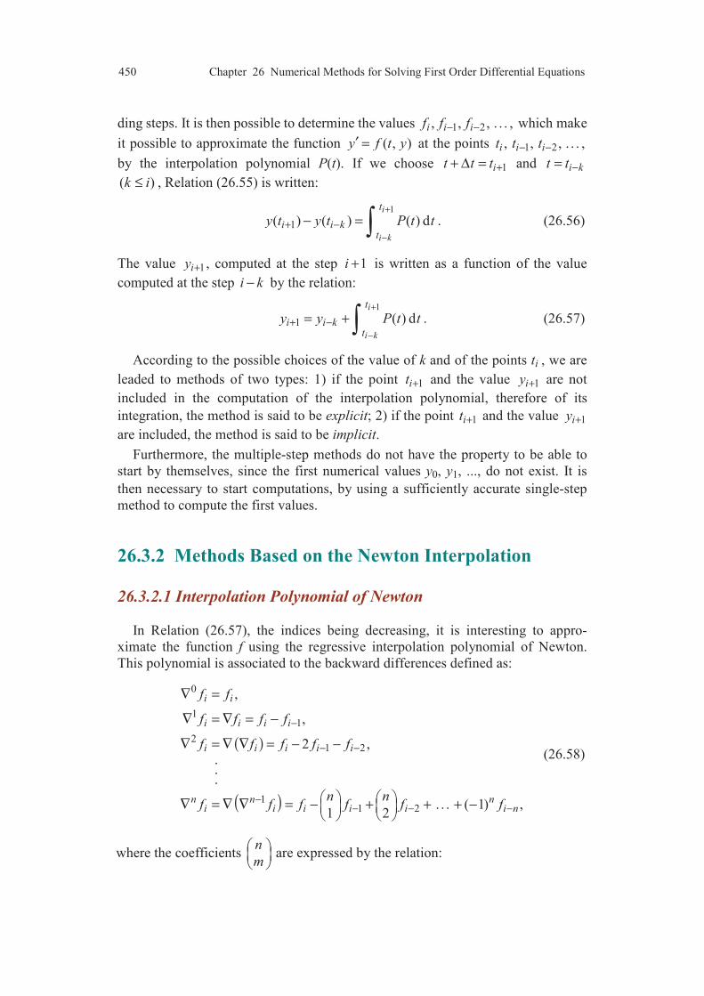
450 Chapter 26 Numerical Methods for Solving First Order Differential Equations
ding steps. It is then possible to determine the values 1 2, , , . . . ,i i if f f− − which make
it possible to approximate the function ( , )y f t y′ = at the points 1 2, , , . . . ,i i it t t− −
by the interpolation polynomial P(t). If we choose 1it t t ++ ∆ = and i kt t −=
( )k i≤ , Relation (26.55) is written:
1
1( ) ( ) ( ) di
i k
t
i i kt
y t y t P t t+
−
+ −− = . (26.56)
The value 1iy + , computed at the step 1i + is written as a function of the value
computed at the step i k− by the relation:
1
1 ( ) di
i k
t
i i kt
y y P t t+
−
+ −= + . (26.57)
According to the possible choices of the value of k and of the points ti , we are
leaded to methods of two types: 1) if the point 1it + and the value 1iy + are not
included in the computation of the interpolation polynomial, therefore of its
integration, the method is said to be explicit; 2) if the point 1it + and the value 1iy +
are included, the method is said to be implicit.
Furthermore, the multiple-step methods do not have the property to be able to
start by themselves, since the first numerical values y0, y1, ..., do not exist. It is
then necessary to start computations, by using a sufficiently accurate single-step
method to compute the first values.
26.3.2 Methods Based on the Newton Interpolation
26.3.2.1 Interpolation Polynomial of Newton
In Relation (26.57), the indices being decreasing, it is interesting to appro-
ximate the function f using the regressive interpolation polynomial of Newton.
This polynomial is associated to the backward differences defined as:
( )
( )
0
11
21 2
11 2
,
,
2 ,...
. . . ( 1) ,1 2
i i
i i i i
i i i i i
n n ni i i i i i n
f f
f f f f
f f f f f
n nf f f f f f
−
− −
−− − −
∇ =
∇ = ∇ = −
∇ = ∇ ∇ = − −
∇ = ∇ ∇ = − + + + −
(26.58)
where the coefficients n
m
are expressed by the relation:
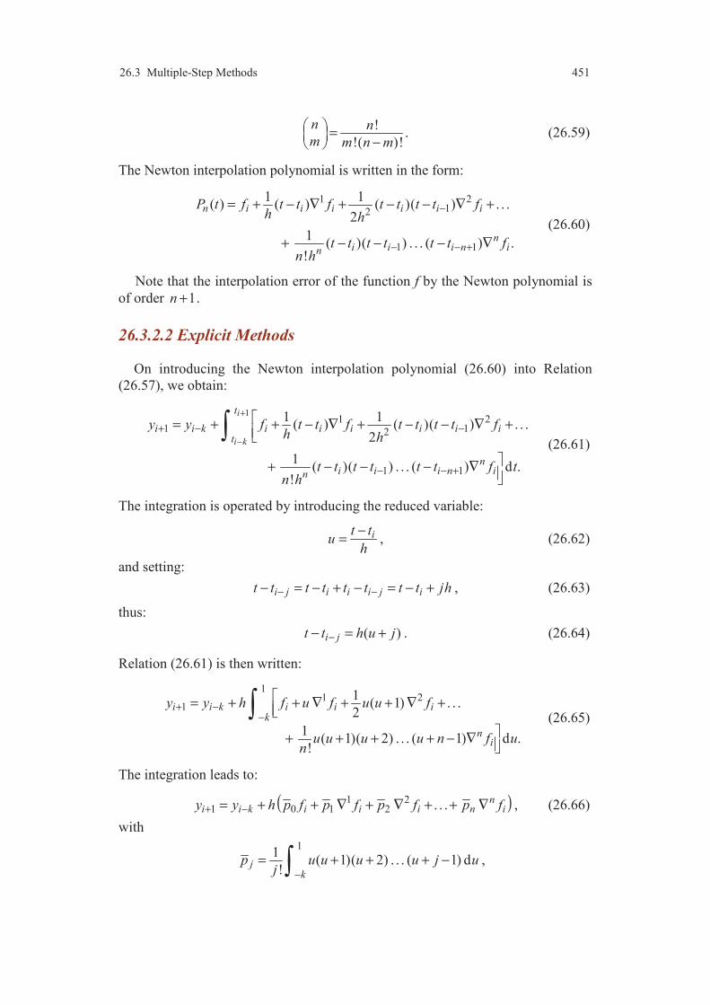
26.3 Multiple-Step Methods 451
!
!( )!
n n
m m n m
= − . (26.59)
The Newton interpolation polynomial is written in the form:
1 212
1 1
1 1( ) ( ) ( )( ) . . .
2
1( )( ) . . . ( ) .
!
n i i i i i i
ni i i n in
P t f t t f t t t t fh h
t t t t t t fn h
−
− − +
= + − ∇ + − − ∇ +
+ − − − ∇
(26.60)
Note that the interpolation error of the function f by the Newton polynomial is
of order 1n + .
26.3.2.2 Explicit Methods
On introducing the Newton interpolation polynomial (26.60) into Relation
(26.57), we obtain:
11 2
1 12
1 1
1 1( ) ( )( ) . . .
2
1( )( ) . . . ( ) d .
!
i
i k
t
i i k i i i i i it
ni i i n in
y y f t t f t t t t fh h
t t t t t t f tn h
+
−
+ − −
− − +
= + + − ∇ + − − ∇ +
+ − − − ∇
(26.61)
The integration is operated by introducing the reduced variable:
it tu
h
−= , (26.62)
and setting:
i j i i i j it t t t t t t t jh− −− = − + − = − + , (26.63)
thus:
( )i jt t h u j−− = + . (26.64)
Relation (26.61) is then written:
11 2
11
( 1) . . .2
1( 1)( 2) . . . ( 1) d .
!
i i k i i ik
ni
y y h f u f u u f
u u u u n f un
+ −−
= + + ∇ + + ∇ +
+ + + + − ∇
(26.65)
The integration leads to:
( ) 1 2
1 0 1 2 . . . ni i k i i i n iy y h p f p f p f p f+ −= + + ∇ + ∇ + + ∇ , (26.66)
with
11
( 1)( 2) . . . ( 1) d!
jk
p u u u u j uj −
= + + + − ,
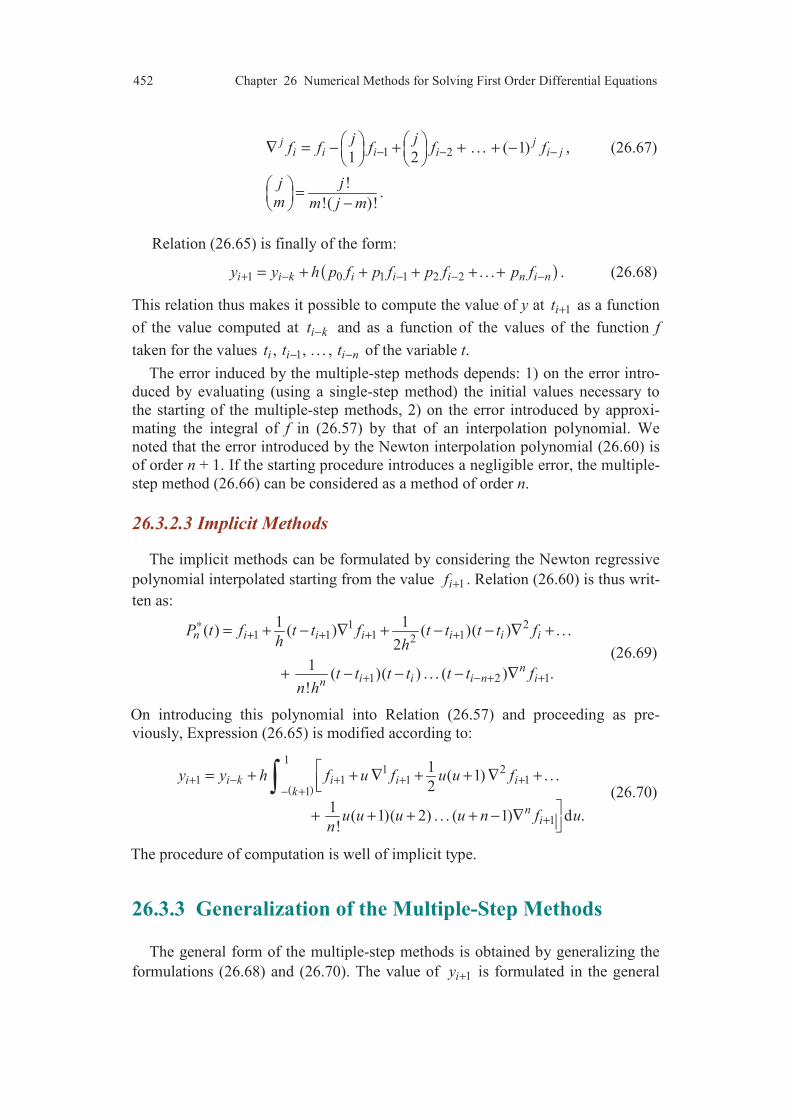
452 Chapter 26 Numerical Methods for Solving First Order Differential Equations
1 2 . . . ( 1)1 2
j ji i i i i j
j jf f f f f− − −
∇ = − + + + −
, (26.67)
!
!( )!
jj
m m j m
= − .
Relation (26.65) is finally of the form:
( ) 1 0 1 1 2 2 . . .i i k i i i n i ny y h p f p f p f p f+ − − − −= + + + + + . (26.68)
This relation thus makes it possible to compute the value of y at 1it + as a function
of the value computed at i kt − and as a function of the values of the function f
taken for the values 1, , . . . ,i i i nt t t− − of the variable t.
The error induced by the multiple-step methods depends: 1) on the error intro-
duced by evaluating (using a single-step method) the initial values necessary to
the starting of the multiple-step methods, 2) on the error introduced by approxi-
mating the integral of f in (26.57) by that of an interpolation polynomial. We
noted that the error introduced by the Newton interpolation polynomial (26.60) is
of order n + 1. If the starting procedure introduces a negligible error, the multiple-
step method (26.66) can be considered as a method of order n.
26.3.2.3 Implicit Methods
The implicit methods can be formulated by considering the Newton regressive
polynomial interpolated starting from the value 1if + . Relation (26.60) is thus writ-
ten as:
1 21 1 1 12
1 2 1
1 1( ) ( ) ( )( ) . . .
2
1( )( ) . . . ( ) .
!
n i i i i i i
ni i i n in
P t f t t f t t t t fh h
t t t t t t fn h
∗+ + + +
+ − + +
= + − ∇ + − − ∇ +
+ − − − ∇
(26.69)
On introducing this polynomial into Relation (26.57) and proceeding as pre-
viously, Expression (26.65) is modified according to:
( )
11 2
1 1 1 11
1
1( 1) . . .
2
1( 1)( 2) . . . ( 1) d .
!
i i k i i ik
ni
y y h f u f u u f
u u u u n f un
+ − + + +− +
+
= + + ∇ + + ∇ +
+ + + + − ∇
(26.70)
The procedure of computation is well of implicit type.
26.3.3 Generalization of the Multiple-Step Methods
The general form of the multiple-step methods is obtained by generalizing the
formulations (26.68) and (26.70). The value of 1iy + is formulated in the general

26.3 Multiple-Step Methods 453
form:
( )1 0 1 1 1 1 0. . . . . .i i i k i k i i k i ky y y y h f f fα α α β β β+ − − − + −= + + + + + + + . (26.71)
If 1 0β− = , the value of 1iy + is deduced from the computed values 1, , . . . ,i if f −
i kf − . The method is explicit. If 1 0β− ≠ , the method is implicit.
After having use a single-step method for starting, an explicit method makes it
possible to compute the value 1iy + as a function of the values evaluated at the pre-
ceding step, using Relation (26.71) with 1 0β− = . Relation (26.71) is thus called
predictor formula. The precision of 1iy + can then be improved by using Relation
(26.71) with 1 0β− ≠ . This process is then implemented using an iterative pro-
cedure. Relation (26.71) is then called corrector formula. Coupling the two for-
mulations leads to a so-called predictor-corrector procedure.
26.3.4 Examples of Multiple-Step Methods
26.3.4.1 Milne Methods
Taking the values 3k = and 2n = , Relation (26.65) is written:
11 2
1 33
1( 1) d .
2i i i i iy y h f u f u u f u+ −
−
= + + ∇ + + ∇ (26.72)
Thus while integrating:
( )
1 21 3
84 4
3i i i i iy y h f f f+ −= + − ∇ + ∇ . (26.73)
Hence, taking account of (26.58):
( )1 3 1 24
2 23
i i i i iy y h f f f+ − − −= + − − (26.74)
This relation is known as the Milne predictor formula.
In the same way, by taking the values 1k = and 2n = , Relation (26.70) is
written:
11 2
1 1 1 1 12
1( 1) d
2i i i i iy y h f u f u u f u+ − + + +
−
= + + ∇ + + ∇ . (26.75)
Thus while integrating:
( )
1 21 1 1 1 1
3 33
2 4i i i i iy y h f f f+ − + + += + − ∇ + ∇ . (26.76)
The introduction of Relations (26.58) transposed to the value fi + 1 leads to:
( ) 1 1 1 14 .3
i i i i ih
y y f f f+ − + −= + + + (26.77)
This relation is known as the Milne corrector formula.
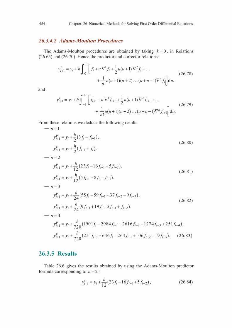
454 Chapter 26 Numerical Methods for Solving First Order Differential Equations
26.3.4.2 Adams-Moulton Procedures
The Adams-Moulton procedures are obtained by taking 0k = , in Relations
(26.65) and (26.70). Hence the predictor and corrector relations:
1p 1 2
10
1( 1) . . .
2
1( 1)( 2) . . . ( 1) d .
!
i i i ii
ni
y y h f u f u u f
u u u u n f un
+= + + ∇ + + ∇ +
+ + + + − ∇
(26.78)
and
0c 1 2
1 1 1 11
1
1( 1) . . .
2
1( 1)( 2) . . . ( 1) d .
!
i i i i i
ni
y y h f u f u u f
u u u u n f un
+ + + +−
+
= + + ∇ + + ∇ +
+ + + + − ∇
(26.79)
From these relations we deduce the following results:
1n =
( )
( )
p11
c1 1
3 ,2
.2
i i ii
i i i i
hy y f f
hy y f f
−+
+ +
= + −
= + +
(26.80)
2n =
( )
( )
p1 21
c1 1 1
23 16 5 ,12
5 8 .12
i i i ii
i i i i i
hy y f f f
hy y f f f
− −+
+ + −
= + − +
= + + −
(26.81)
3n =
( )
( )
p1 2 31
c1 1 1 2
55 59 37 9 ,24
9 19 5 .24
i i i i ii
i i i i i i
hy y f f f f
hy y f f f f
− − −+
+ + − −
= + − + −
= + + − +
(26.82)
4n =
( )
( )
p1 2 3 41
c1 1 1 2 3
1901 2984 2616 1274 251 ,720
251 646 264 106 19 . (26.83)720
i i i i i ii
i i i i i i i
hy y f f f f f
hy y f f f f f
− − − −+
+ + − − −
= + − + − +
= + + − + −
26.3.5 Results
Table 26.6 gives the results obtained by using the Adams-Moulton predictor
formula corresponding to 2n = :
( )p1 21 23 16 5
12i i i ii
hy y f f f− −+ = + − + , (26.84)

26.3 Multiple-Step Methods 455
TABLE 26.6 Results derived from an Adams-Moulton predictor procedure, for three
values of the step of computation.
variable t 1 2 3 4 5
yexact 1 2.82842712 7.02113212 14.69693846 27.00000000
h = 0.10 yi 1 2.82835406 7.02101203 14.69677999 26.99980445
error 0 – 0.00007306 – 0.00012009 – 0.00015847 – 0.00019555
h = 0.05 yi 1 2.82841644 7.02111523 14.69691628 26.99997266
error 0 – 0.00001069 – 0.00001690 – 0.00002218 – 0.00002734
h = 0.01 yi 1 2.82842703 7.02113197 14.69693826 26.99999976
error 0 – 0.00000009 – 0.00000015 – 0.00000019 – 0.00000024
for solving the differential equation (26.6). The starting procedure, used to
compute the first three values, is the Runge-Kutta method of order 4. The results
obtained for the different values of the step ( 0.10,h = 0.05h = and 0.01h = )
show that the procedure is appreciably of the third order.
The precision can be improved by associating to the predictor formula a
corrector formula of the same order. The precision of the result could then be
possibly controlled by using an iterative corrector process until the difference
obtained between two successive corrections is acceptable.
Table 26.7 shows the results obtained by associating to the predictor formula
(26.84) the corrector formula:
( )c1 1 1 29 19 5
24i i i i i i
hy y f f f f+ + − −= + + − + . (26.85)
TABLE 26.7 Results obtained by an Adams-Moulton predictor-corrector procedure, for a
step of h = 0.2 and in the case of several successive corrections k.
variable t 1 2 3 4 5
yexact 1 2.82842712 7.02113212 14.69693846 27.00000000
k = 0 yi 1 2.82801553 7.02037351 14.69592343 26.99874364
error 0 – 0.00041160 – 0.000758610 – 0.001015029 – 0.001256356
k = 1 yi 1 2.82840571 7.02109451 14.69688877 26.99993877
error 0 – 0.00002141 – 0.00003762 – 0.00004969 – 0.00006123
k = 2 yi 1 2.82841553 7.02111213 14.69691211 26.99996754
error 0 – 0.00001160 – 0.00001999 – 0.00002635 – 0.00003246
k = 5 yi 1 2.82841579 7.02111259 14.69691271 26.99996827
erreur 0 - 0.00001134 - 0.00001953 - 0.00002575 - 0.00003172

456 Chapter 26 Numerical Methods for Solving First Order Differential Equations
Table 26.7 compares, for a step of computation 0.20,h = the results obtained
without correction ( 0k = ) to the results obtained k with successive corrections
( 1k = , 2k = and 5k = ) at each step of computation. The results show that the
precision is clearly improved when one correction is used (the error obtained for
5t = is appreciably divided by 20). However, the improvement is then limited,
when the number of successive corrections is increased.
EXERCISES
26.1 Establish Relations (26.37) and (26.38) which are obtained in the case of the
Runge-Kutta methods of order 4.
26.2 Implement the numerical procedures, using the different methods consi-
dered in this chapter, to solve the differential equation:
2d2
d
yty
t= −
in the interval [ ]0, 2t ∈ , with the initial value (0) 1y = .
COMMENTS
The numerical methods constitute an indispensable tool for solving the
differential equations. In a first approach, the reader will be interested in
the Euler-Cauchy method, then in the Runge-Kutta methods of order 4.
Then, the reader will study thoroughly the methods which make it
possible to control the precision of the computation.
The implementation of the different methods will be carried out by the
reader by deriving the results reported in the different tables of this
chapter.
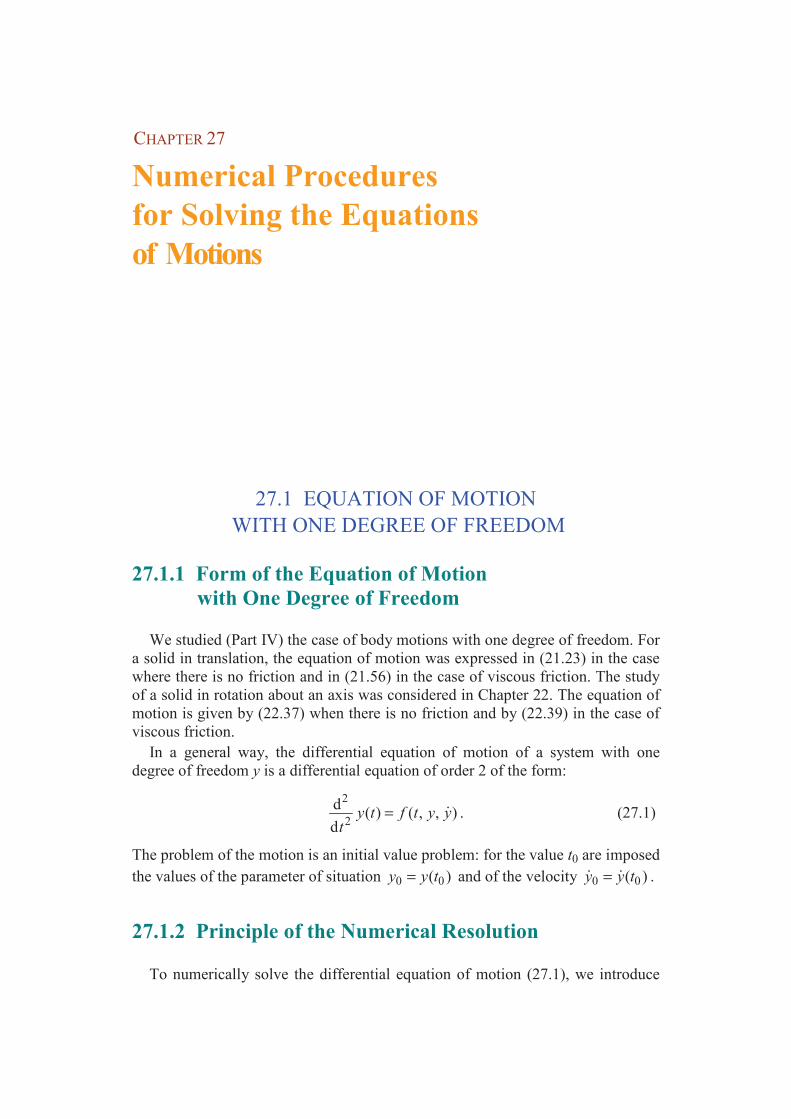
CHAPTER 27
Numerical Procedures for Solving the Equations of Motions
27.1 EQUATION OF MOTION
WITH ONE DEGREE OF FREEDOM
27.1.1 Form of the Equation of Motion with One Degree of Freedom
We studied (Part IV) the case of body motions with one degree of freedom. For
a solid in translation, the equation of motion was expressed in (21.23) in the case
where there is no friction and in (21.56) in the case of viscous friction. The study
of a solid in rotation about an axis was considered in Chapter 22. The equation of
motion is given by (22.37) when there is no friction and by (22.39) in the case of
viscous friction.
In a general way, the differential equation of motion of a system with one
degree of freedom y is a differential equation of order 2 of the form:
2
2
d( ) ( , , )
dy t f t y y
t= . (27.1)
The problem of the motion is an initial value problem: for the value t0 are imposed
the values of the parameter of situation 0 0( )y y t= and of the velocity 0 0( )y y t= .
27.1.2 Principle of the Numerical Resolution
To numerically solve the differential equation of motion (27.1), we introduce
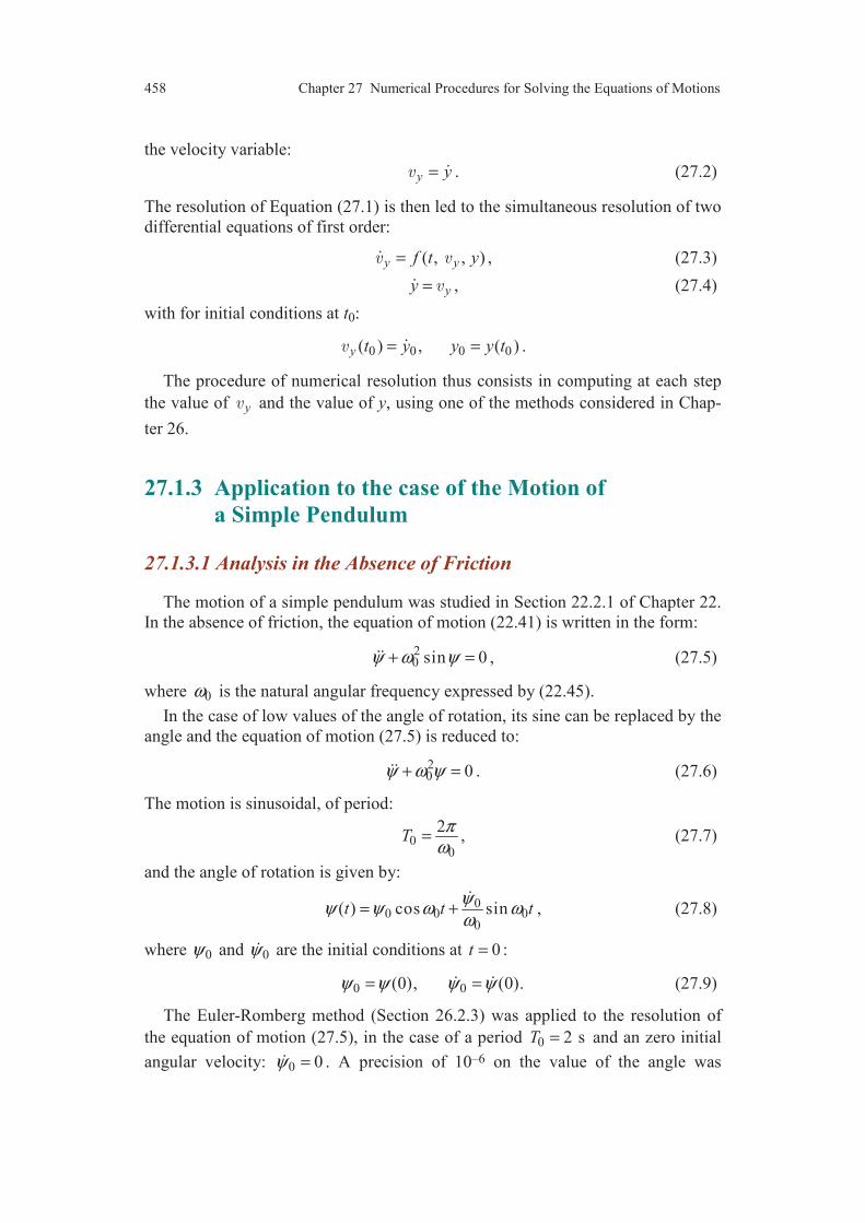
458 Chapter 27 Numerical Procedures for Solving the Equations of Motions
the velocity variable:
y y= . (27.2)
The resolution of Equation (27.1) is then led to the simultaneous resolution of two
differential equations of first order:
( , , )y yf t y= , (27.3)
yy = , (27.4)
with for initial conditions at t0:
0 0 0 0( ) , ( )y t y y y t= = .
The procedure of numerical resolution thus consists in computing at each step
the value of y and the value of y, using one of the methods considered in Chap-
ter 26.
27.1.3 Application to the case of the Motion of a Simple Pendulum
27.1.3.1 Analysis in the Absence of Friction
The motion of a simple pendulum was studied in Section 22.2.1 of Chapter 22.
In the absence of friction, the equation of motion (22.41) is written in the form:
20 sin 0ψ ω ψ+ = , (27.5)
where 0ω is the natural angular frequency expressed by (22.45).
In the case of low values of the angle of rotation, its sine can be replaced by the
angle and the equation of motion (27.5) is reduced to:
20 0ψ ω ψ+ = . (27.6)
The motion is sinusoidal, of period:
00
2T
πω
= , (27.7)
and the angle of rotation is given by:
00 0 0
0
( ) cos sint t tψ
ψ ψ ω ωω
= +
, (27.8)
where 0ψ and 0ψ are the initial conditions at 0t = :
0 0(0), (0).ψ ψ ψ ψ= = (27.9)
The Euler-Romberg method (Section 26.2.3) was applied to the resolution of
the equation of motion (27.5), in the case of a period 0 2 sT = and an zero initial
angular velocity: 0 0ψ = . A precision of 10–6 on the value of the angle was
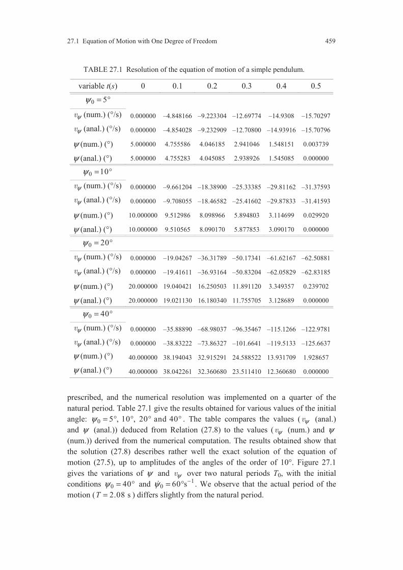
27.1 Equation of Motion with One Degree of Freedom 459
TABLE 27.1 Resolution of the equation of motion of a simple pendulum.
variable t(s) 0 0.1 0.2 0.3 0.4 0.5
0 5ψ = °
ψ (num.) (°/s) 0.000000 –4.848166 –9.223304 –12.69774 –14.9308 –15.70297
ψ (anal.) (°/s) 0.000000 –4.854028 –9.232909 –12.70800 –14.93916 –15.70796
ψ (num.) (°) 5.000000 4.755586 4.046185 2.941046 1.548151 0.003739
ψ (anal.) (°) 5.000000 4.755283 4.045085 2.938926 1.545085 0.000000
0 10ψ = °
ψ (num.) (°/s) 0.000000 –9.661204 –18.38900 –25.33385 –29.81162 –31.37593
ψ (anal.) (°/s) 0.000000 –9.708055 –18.46582 –25.41602 –29.87833 –31.41593
ψ (num.) (°) 10.000000 9.512986 8.098966 5.894803 3.114699 0.029920
ψ (anal.) (°) 10.000000 9.510565 8.090170 5.877853 3.090170 0.000000
0 20ψ = °
ψ (num.) (°/s) 0.000000 –19.04267 –36.31789 –50.17341 –61.62167 –62.50881
ψ (anal.) (°/s) 0.000000 –19.41611 –36.93164 –50.83204 –62.05829 –62.83185
ψ (num.) (°) 20.000000 19.040421 16.250503 11.891120 3.349357 0.239702
ψ (anal.) (°) 20.000000 19.021130 16.180340 11.755705 3.128689 0.000000
0 40ψ = °
ψ (num.) (°/s) 0.000000 –35.88890 –68.98037 –96.35467 –115.1266 –122.9781
ψ (anal.) (°/s) 0.000000 –38.83222 –73.86327 –101.6641 –119.5133 –125.6637
ψ (num.) (°) 40.000000 38.194043 32.915291 24.588522 13.931709 1.928657
ψ (anal.) (°) 40.000000 38.042261 32.360680 23.511410 12.360680 0.000000
prescribed, and the numerical resolution was implemented on a quarter of the
natural period. Table 27.1 give the results obtained for various values of the initial
angle: 0 5 , 10 , 20 and 40ψ = ° ° ° ° . The table compares the values ( ψ (anal.)
and ψ (anal.)) deduced from Relation (27.8) to the values ( ψ (num.) and ψ
(num.)) derived from the numerical computation. The results obtained show that
the solution (27.8) describes rather well the exact solution of the equation of
motion (27.5), up to amplitudes of the angles of the order of 10°. Figure 27.1
gives the variations of ψ and ψ over two natural periods T0, with the initial
conditions 0 40ψ = ° and 10 60 sψ −= ° . We observe that the actual period of the
motion ( 2.08 sT = ) differs slightly from the natural period.

460 Chapter 27 Numerical Procedures for Solving the Equations of Motions
temps ( s )
0 1 2 3 4 5 6 7 8 9 10
ang
le d
e ro
tati
on (
° )
-50
-40
-30
-20
-10
0
10
20
30
40
50
temps ( s )
0 1 2 3 4 5 6 7 8 9 10
ang
le d
e ro
tati
on
(
° )
-50
-40
-30
-20
-10
0
10
20
30
40
50
FIGURE 27.1 Motion of a simple pendulum, for the initial conditions 0 40ψ = ° and
0 60 /sψ = ° .
FIGURE 27.2. Motion of a simple pendulum as a function of time, for four values of the
damping.
temps ( s )0 1 2 3 4
angle
de
rota
tio
n
ψ
( °
)
-40
-20
0
20
40
-160
vitesse d
e rotatio
n ψ
( °/s )
-80
160
80
0
angle of rotation
rotation velocity ang
le o
f ro
tati
on
(°
)
rotatio
n v
elocity
ψ
( °/s )
time ( s )
temps ( s )
0 1 2 3 4 5 6 7 8 9 10
angle
de
rota
tio
n (
° )
-50
-40
-30
-20
-10
0
10
20
30
40
50
temps ( s )
0 1 2 3 4 5 6 7 8 9 10
angle
de
rota
tion
(
° )
-50
-40
-30
-20
-10
0
10
20
30
40
50
= 0.25 s−1
= 1 s−1
= 3.14 s−1
= 5 s−1
time ( s ) time ( s )
time ( s ) time ( s )
ang
le o
f ro
tati
on
( °
)
ang
le o
f ro
tati
on
( °
)
ang
le o
f ro
tati
on
( °
)
ang
le o
f ro
tati
on
( °
)

27.2 Equations of Motions with Several Degrees of Freedom 461
27.1.3.2 Analysis in the Presence of Friction
In the case of a friction of viscous type, the equation of motion (22.50) is:
202 sin 0ψ δψ ω ψ+ + = . (27.10)
For low values of the angle of rotation, the equation of motion is reduced to
Equation (22.52), which is the reduced form for a system with one degree of
freedom with viscous friction. The free vibrations were studied in Section 21.3.2
of Chapter 21. For a natural period 0 2 sT = , the critical damping is (21.91): 13.1416 scδ −= .
Figures 27.2 report the results derived from a numerical resolution of Equation
(27.10) using the Runge-Kutta method of order 4. Four values for the damping
are considered: 0.25 s–1, 1 s–1, 3.1416 s–1 and 5 s–1, with the initial conditions:
0 40ψ = ° and 10 60 sψ −= ° . We find well the different types of motions studied in
Section 21.3.2.
27.2 EQUATIONS OF MOTIONS WITH SEVERAL
DEGREES OF FREEDOM
27.2.1 Form of the Equations of Motions with Several Degrees of Freedom
In the general case, the motion of a solid or a system of solids is a motion with
several degrees of freedom. Various motions were studied in Chapters 23 to 25.
The equations of motions are either deduced from the fundamental principle of
dynamics, or obtained automatically using the Lagrange equations. For a mecha-
nical system having p degrees of freedom de: y1, y2, ..., yp, the equations of
motions are written in the general form:
1 1 1 1 2 2
2 2 1 1 2 2
1 1 2 2
( , , , , , . . . , , ),
( , , , , , . . . , , ),...
( , , , , , . . . , , ),
p p
p p
p p p p
y f t y y y y y y
y f t y y y y y y
y f t y y y y y y
=
=
=
(27.11)
with the initial conditions:
0 0
0 0( ) , ( ) , 1, 2, . . . , .i i i iy t y y t y i p= = = (27.12)

462 Chapter 27 Numerical Procedures for Solving the Equations of Motions
27.2.2 Principle of the Numerical Resolution
We have to solve a system (27.11) of p differential equations of the second
order. To solve it numerically, we generalize the method used in Section 27.1.2
for the numerical resolution of the equation of the motion of a system with one
degree of freedom. For that, we introduce the variables:
, 1, 2, . . . , ,iy iy i p= = (27.13)
and we lead the system of the p equations of the second order to a system of 2p
differential equations of the first order:
1
1 1 2
2
2 1 2
1 2
1
1 1 2
2
2 1 2
1 2
,
( , , , , , . . . , , ),
,
( , , , , , . . . , , ),...
,
( , , , , , . . . , , ),
p
p
p
p p
y
y y y p y
y
y y y p y
p y
y p y y p y
y
f t y y y
y
f t y y y
y
f t y y y
=
=
=
=
=
=
(27.14)
with the initial conditions:
0 0
0 0( ) , ( ) , 1, 2, . . . , .i ii i y yy t y t i p= = = (27.15)
The procedure of numerical resolution consists in computing at each step, using
one of the methods considered in Chapter 26, the values of 1 2, ,..., ,py y y and
the values of y1, y2, ..., yp.
27.2.3 Trajectories and Kinematic Vectors
Once solved the equations of motion, the trajectories and the kinematic vectors
of an arbitrary point of a solid are obtained as functions of the parameters of
situation, in accordance to the results of the kinematics of the solid (Chapter 9).
The trajectory of an arbitrary point M of the solid (S) in motion with respect to the
reference (T) is obtained by Relation (9.5):
t
( , ) ( , ) ( )
( , ) ( , ) ( ) ( )
( , ) ( , ) ( )
S
S
S
x M t x P t x M
y M t y P t t y M
z M t z P t z M
= +
A . (27.16)
trajectory of deduced from coordinates of the point M
the point M in the parameters of in a system attached to (S)
the reference (T) situation y1, y2, ... yp and of origin P
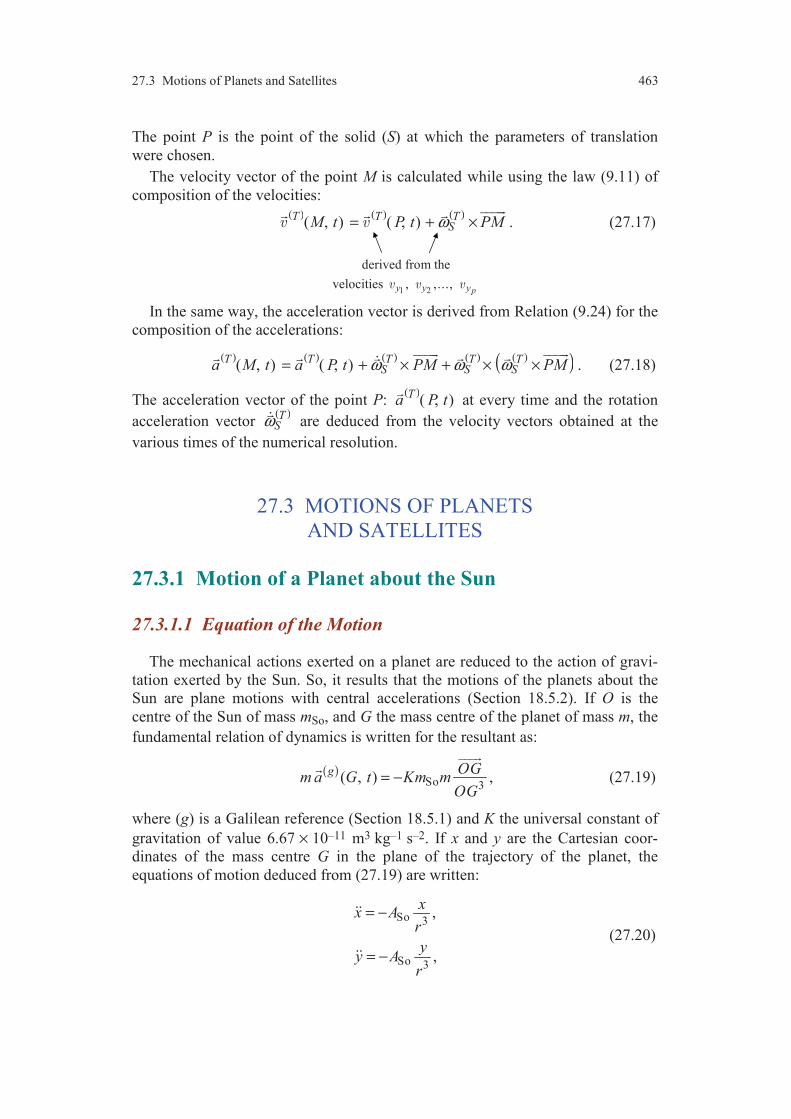
27.3 Motions of Planets and Satellites 463
The point P is the point of the solid (S) at which the parameters of translation
were chosen.
The velocity vector of the point M is calculated while using the law (9.11) of
composition of the velocities: ( ) ( ) ( )
( , ) ( , )T T TSM t P t PMω= + ×
. (27.17)
derived from the
velocities 1 2, ,...,
py y y
In the same way, the acceleration vector is derived from Relation (9.24) for the
composition of the accelerations:
( ) ( ) ( ) ( ) ( )( ) ( , ) ( , )T T T T TS S Sa M t a P t PM PMω ω ω= + × + × ×
. (27.18)
The acceleration vector of the point P: ( )
( , )Ta P t
at every time and the rotation
acceleration vector ( )TSω are deduced from the velocity vectors obtained at the
various times of the numerical resolution.
27.3 MOTIONS OF PLANETS
AND SATELLITES
27.3.1 Motion of a Planet about the Sun
27.3.1.1 Equation of the Motion
The mechanical actions exerted on a planet are reduced to the action of gravi-
tation exerted by the Sun. So, it results that the motions of the planets about the
Sun are plane motions with central accelerations (Section 18.5.2). If O is the
centre of the Sun of mass mSo, and G the mass centre of the planet of mass m, the
fundamental relation of dynamics is written for the resultant as:
( )So 3
( , )g OG
m a G t Km mOG
= −
, (27.19)
where (g) is a Galilean reference (Section 18.5.1) and K the universal constant of
gravitation of value 6.67 × 10⁻¹¹ m3 kg–1 s–2. If x and y are the Cartesian coor-
dinates of the mass centre G in the plane of the trajectory of the planet, the
equations of motion deduced from (27.19) are written:
So 3
So 3
,
,
xx A
r
yy A
r
= −
= −
(27.20)

464 Chapter 27 Numerical Procedures for Solving the Equations of Motions
FIGURE 27.3. Plane of the trajectory of a planet.
where r is the distance between the points O and G (Figure 27.3):
2 2r x y= + , (27.21)
and ASo is a constant expressed by:
So SoA Km= . (27.22)
With a mass of the Sun appreciably equal to 302 10 kg× , the value of this cons-
tant is: 19 3 2So 13.34 10 m sA −= × .
27.3.1.2 Numerical Resolution of the Equations of Motion
To numerically solve Equations (27.20) of motion, it is interesting to use a
constant step of length of the trajectory, rather than a constant step of time. A
constant step of trajectory makes it possible to have an appreciably constant
computation time throughout the trajectory. As input of the numerical procedure,
we introduce the step hs of curvilinear abscissa corresponding to a given length of
the trajectory. The step in time is then calculated at every moment by the relation:
shh =
, (27.23)
where is the instantaneous velocity at the moment under consideration.
27.3.1.3 Examples of Results
As an example, we consider the case of a planet which would have at 0,t = a
position G0 of Cartesian coordinates 80 0 0( 1.5 10 km, 0, 0)x y z= − × = = and a
velocity 0
of components 1
0 0 0( 0, 20 km s , 0)x y z−= = = .
For solving the equations of the motion, we use the Euler method with a
computation step equal to 100,000 km. The computation is stopped when the
planet reaches its initial position G0. Figure 27.4a shows the trajectory obtained.
The step chosen for the computation is in fact relatively low, since the total
y
x
G
r
O
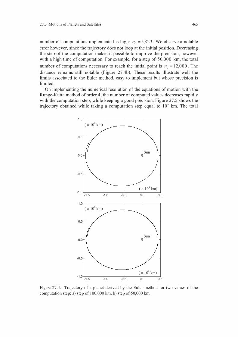
27.3 Motions of Planets and Satellites 465
-1,5 -1,0 -0,5 0,0 0,5-1,0
-0,5
0,0
0,5
1,0
( × 108 km)
( × 108 km)
Sun
-1.5 -1.0 -0.5 0.0 0.5 -1.0
-0.5
0.0
0.5
1.0
-1,5 -1,0 -0,5 0,0 0,5-1,0
-0,5
0,0
0,5
1,0
( × 108 km)
( × 108 km)
Sun
-1.5 -1.0 -0.5 0.0 0.5 -1.0
-0.5
0.0
0.5
1.0
number of computations implemented is high: 5,823cn = . We observe a notable
error however, since the trajectory does not loop at the initial position. Decreasing
the step of the computation makes it possible to improve the precision, however
with a high time of computation. For example, for a step of 50,000 km, the total
number of computations necessary to reach the initial point is 12,000cn = . The
distance remains still notable (Figure 27.4b). These results illustrate well the
limits associated to the Euler method, easy to implement but whose precision is
limited.
On implementing the numerical resolution of the equations of motion with the
Runge-Kutta method of order 4, the number of computed values decreases rapidly
with the computation step, while keeping a good precision. Figure 27.5 shows the
trajectory obtained while taking a computation step equal to 107 km. The total
FIgure 27.4. Trajectory of a planet derived by the Euler method for two values of the
computation step: a) step of 100,000 km, b) step of 50,000 km.

466 Chapter 27 Numerical Procedures for Solving the Equations of Motions
-1,5 -1,0 -0,5 0,0 0,5 1,0 1,5
-1,5
-1,0
-0,5
0,0
0,5
1,0
1,5( × 10
8 km)
( × 108 km)
Sun
-1.0
-0.5
0.0
0.5
1.0
1.5
-1.5
-1.5 -1.0 -0.5 0.0 0.5 1.5 1.0
FIGURE 27.5. Trajectory of a planet derived by the Runge-Kutta method of order 4, with
a computation step of 107 km.
number of computations to reach the initial point is 56cn = . The trajectory loops
well at its initial point in this case. This result shows thus the interest to use a
resolution method of high order.
By modifying the initial velocity of the preceding example according to
0( 0,x = 10 030 km s , 0)y z−= = , the trajectory obtained by the Runge-Kutta
method is the one of Figure 27.6. This trajectory is fairly the one of the Earth
about the Sun (elliptic trajectory of semi-major axis equal to 81.496 10× km and
eccentricity equal to 0.017).
FIGURE 27.6 Trajectory obtained by the Runge-Kutta method of order 4, with for initial
conditions 80 ( 1.5 10 km, 0, 0)G − × and 1
0 (0, 30 km s , 0).−
-1,5 -1,0 -0,5 0,0 0,5-1,0
-0,5
0,0
0,5
1,0
( × 108 km)
Sun
( × 108 km)
-1.0
-0.5
0.0
0.5
1.0
-1.5 -1.0 -0.5 0.0 0.5

27.3 Motions of Planets and Satellites 467
-1,0 -0,5 0,0 0,5 1,0 1,5
-1,0
-0,5
0,0
0,5
1,0
Ea
h t r
( × 104 km )
( × 104 km )
(a)
(b) (c)
(d)
(a): 6 km/h
(b): 7 km/h
(c): 7.4 km/h
(d): 7.8 km/h
-1.0 -0.5 0.0 0.5 1.5 1.0
-1.0
-0.5
0.0
0.5
1.0
27.3.2 Motion of a Satellite around the Earth
In the case of the motion of a satellite in the vicinity of the Earth, the mecha-
nical actions exerted on the satellite are reduced to the action of gravitation
exerted by the Earth. The fundamental relation of dynamics for the resultant is
transposed from Relation (27.19), thus:
( )TeTe 3
( , )OG
m a G t Km mOG
= −
, (27.24)
where (Te) is a reference attached to the plane of the ecliptic, mTe is the mass of
the Earth, O its centre and G the mass centre of the satellite of mass m. If x and y
are the Cartesian coordinates of the mass centre G in the plane of the trajectory of
the satellite, the equations of the motion have the same form as Equation (27.20),
thus:
Te 3
Te 3
,
,
xx A
r
yy A
r
= −
= −
(27.25)
where the constant ATe is expressed by:
Te TeA Km= . (27.26)
With a mass of the Earth fairly equal to 246 10× kg, the value of this constant is:
13 3 2
Te 40.02 10 m sA −= × .
Figure 27.7 shows the trajectories computed by the Runge-Kutta method of
FIGURE 27.7. Trajectories computed for a satellite launched at the point
8
0 ( 1.5 10 km, 0, 0)G − × with an initial velocity 0(0, , 0)y , for four values of 0y .
468 Chapter 27 Numerical Procedures for Solving the Equations of Motions
order 4 with a step of 100 km, for a satellite launched at the point G0 with an
initial velocity of components 0(0, , 0)y . Four values of the component 0y are
considered: 16, 7, 7.4 and 7.8 km s− . The results obtained show the influence of
the launching velocity. In the case where the component is equal to 6 km s– 1, the
launching velocity is not high enough, and the satellite is crashed on the surface
of the Earth after its launching. For a value of the component of 7 km s– 1, the
orbit is slightly eccentric, the satellite keeping a rather constant altitude. The
increase of the value of the component enhances then the eccentricity of the
ellipse.
27.3.3 Launching and Motion of a Moon Probe
In this subsection, we consider the motion of a Moon probe launched from a
earthly orbit. Launched from this orbit, the objective is that the probe turns around
the Moon, then returns in the vicinity of the Earth to be recovered. Furthermore,
its recovery needs a return in the atmosphere under a favourable angle.
The equation of motion of the mass centre G of the probe is written:
( ) Te LTe L3 3
Te L
( , )T O G O Ga G t K m m
r r
= − +
, (27.27)
where OTe and OL are the respective centres of the Earth and of the Moon, mTe
and mL (mL = 227.4 10 kg× ) the respective masses of the Earth and of the Moon,
and rTe and rL the distances from the probe respectively to the Earth and to the
Moon. If (x, y) are the Cartesian coordinates of the probe in the plane of its tra-
jectory (figure 27.8), Equation (27.27) leads to the equations of motion:
LTe L3 3
Te L
Te L3 3Te L
,
,
x xxx K m m
r r
y yy K m m
r r
− = − +
= − +
(27.28)
with
( )22 2 2Te L L, ,r x y r x x y= + = − +
and where xL is the distance from the Moon to the Earth (xL = 384,000 km). For
reasons of simplicity, the equations do not take into account the relative motion of
the Moon with respect to the Earth. This motion can be taken into account
without difficulty, in the case of a numerical procedure.
The examples considered (Figure 27.9) use the same initial position for the
launching ,( 19 000 km, 0, 0)− with initial velocities directed along the direction
Oy
of component 0y having various values. The trajectories were computed,
using the Runge-Kutta method of order 4 and choosing a step of 1,000 km.

27.4 Motion of a Solid on an Inclined Plane 469
FIGURE 27.8. Coordinates of the probe in the plane of its trajectory.
We observe (Figure 27.9a) that for the lowest velocities of launching (6 to 6.25
km s–1), the trajectories stay in the vicinity of the Earth and the influence of the
Moon is negligible. It appears only for 10 6.30 km sy −= .
Figure 27.9b shows two trajectories: the one where the probe escapes the Moon
attraction ( 10 6.40 km sy −= ) and the other ( 1
0 6.3155 km sy −= ) corresponding
to an ideal launching, with passing round the Moon and return in the vicinity of
the Earth
Figure 27.9c shows the notable influence on the trajectories of low variations of
the launching velocity at the vicinity of the ideal trajectory: for 0y = 16.30 km s−
the probe does not reach the vicinity of the Moon, for 0y = 6.33 km s–1 the probe
is crashed on the Moon, for 10 6.35 km sy −= the probe passes behind the Moon
and returns at the vicinity of the Earth.
Lastly, Figure 27.9d shows a complex trajectory of the probe, obtained for 1
0 6.31 km sy −= . Arrived in the vicinity of the Moon, the probe starts to pass
around the Moon in the direct direction, then it continues to turn around in the
inverse direction, to return then on the Earth.
In practice, the satellites are provided with auxiliary engines which make it
possible to correct the variations of the trajectory at every moment.
27.4 MOTION OF A SOLID ON AN INCLINED PLANE
The equations of motion on a solid on an inclined plane have been expressed in
(23.43) in the case of viscous friction:
sin ,
0,
0,
t
t
r
mx c x mg
my c y
C c
α
ψ ψ
+ =
+ =
+ =
(27.29)
where ct and cr are the coefficients of viscous friction in translation and rotation,
y
x
G
rTe
OTe
rL
xL
L

470 Chapter 27 Numerical Procedures for Solving the Equations of Motions
0,0 0,5 1,0 1,5 2,0 2,5 3,0 3,5 4,0
-1,0
-0,5
0,0
0,5
1,0
Earth Moon
( × 105 km )
( × 105 km )
0 6.31 km/sy =
(d) 2.0 1.5 2.5 3.0 3.5 4.0 1.0 0.5 0.0
0.0
-0.5
-1.0
1.0
0.5
0,0 0,5 1,0 1,5 2,0 2,5 3,0 3,5 4,0
-1,0
-0,5
0,0
0,5
1,0
Earth Moon
( × 105 km )
( × 105 km )
(a) (b) (c)
(a): 0 6.30 km/sy =
(b): 0 6.33 km/sy =
(c): 0 6.35 km/sy =
2.0 1.5 2.5 3.0 3.5 4.0 1.0 0.5 0.0
0.0
-0.5
-1.0
1.0
0.5
0,0 0,5 1,0 1,5 2,0 2,5 3,0 3,5 4,0
-1,0
-0,5
0,0
0,5
1,0
Earth Moon
( × 105 km )
( × 105 km )
(a)
(b)
(a): 0 6.3155 km/sy =
(b): 0 6.5000 km/sy =
0.0
-0.5
-1.0
1.0
0.5
2.0 1.5 2.5 3.0 3.5 4.0 1.0 0.5 0.0
0,0 0,5 1,0 1,5 2,0 2,5 3,0 3,5 4,0
-1,0
-0,5
0,0
0,5
1,0
Earth Moon
( × 105 km )
( × 105 km )
(a) (b) (c) (d) (e)
(a): 0 6.00 km/sy =
(b): 0 6.10 km/sy =
(c): 0 6.20 km/sy =
(d): 0 6.25 km/sy =
(e): 0 6.30 km/sy =
2.0 1.5 2.5 3.0 3.5 4.0 1.0 0.5 0.0
0.0
-0.5
-1.0
1.0
0.5
FIGURE 27.9 Trajectories of a Moon probe launched from the position (–19,000 km, 0,
0) with various initial velocities.
(a)
(b)
(c)

27.4 Motion of a Solid on an Inclined Plane 471
respectively. In reduced forms these equations are written:
sin ,
,
,
t
t
r
x g f x
y f y
f
α
ψ ψ
= −
= −
= −
(27.30)
introducing the viscous damping coefficients in translation and rotation:
, .t rt r
c cf f
m m= = (27.31)
Note that the x-axis is the direction of greater slope of the inclined plane.
The equations (27.30) are solved numerically using for example the Runge-
Kutta method of order 4. The resolution makes it possible to derive the para-
meters of situation x, y, ψ, and their derivatives , , x y ψ as functions of time. The
trajectory of the mass centre is deduced from the parameters (x, y). Then, it is
possible to obtain the trajectory of an arbitrary point of the solid by using Relation
(27.16).
Figures 27.10 show the results obtained for various values of the inclination of
the plane and of the damping coefficients ft and fr. At the initial moment ( 0),t =the mass centre is at the origin point of the coordinate system and has a velocity
vector 10 (0, 5 m s , 0)− . At 0t = , the orientation of the coordinate system
attached to the solid coincides with the one of the system attached to the inclined
plane (Section 23.2.1) and the angular velocity is taken as 10 360 sψ −= ° . Com-
putations were implemented in the interval [0, 5 s], with a computation step equal
to 0.05 s. In Figures 27.10, are reported the trajectories of the mass centre and of a
point attached to the solid of coordinates (4 m, 0, 0) relatively to the system
attached to the solid. The results obtained show the influence of the angle of
inclination of the plane, and the influence of the frictions in translation and
rotation.
27.5 COUPLED MOTIONS OF TWO SOLIDS
27.5.1 Equations of Motion
In this section we return to the motion of the two solids considered in Section
24.3 of Chapter 24. In the case of a viscous friction, the equations of motion have
been written in (24.120):
( ) ( ) ( )21 2 0 2
2 2 2
cos sin 0,
cos sin 0.
t
r
m m y c y k y d l m a
m ay C c m ga
ψ ψ ψ ψ
ψ ψ ψ ψ
+ + + − − + − =
+ + + =
(27.32)
The motion of the solid (S1) is induced around the position of equilibrium
0y l d= + . Hereafter, we study the motion around this equilibrium introducing
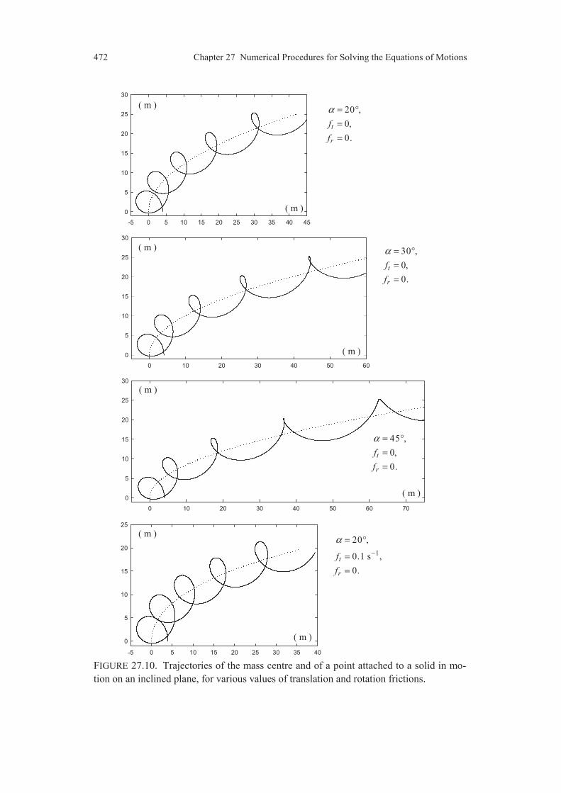
472 Chapter 27 Numerical Procedures for Solving the Equations of Motions
-5 0 5 10 15 20 25 30 35 40
0
5
10
15
20
25
0 10 20 30 40 50 60 70
0
5
10
15
20
25
30
0 10 20 30 40 50 60
0
5
10
15
20
25
30
-5 0 5 10 15 20 25 30 35 40 45
0
5
10
15
20
25
30
FIGURE 27.10. Trajectories of the mass centre and of a point attached to a solid in mo-
tion on an inclined plane, for various values of translation and rotation frictions.
( m )
( m )
( m )
( m )
( m )
( m )
( m )
( m )
20 ,
0,
0.
t
r
f
f
α = °
=
=
30 ,
0,
0.
t
r
f
f
α = °
=
=
45 ,
0,
0.
t
r
f
f
α = °
=
=
1
20 ,
0.1 s ,
0.
t
r
f
f
α−
= °
=
=

27.4 Motion of a Solid on an Inclined Plane 473
-5 0 5 10 15 20 25
0
2
4
6
8
10
12
14
-5 0 5 10 15 20 25
0
2
4
6
8
10
12
14
-5 0 5 10 15 20 25 30 35 40
0
5
10
15
20
25
-5 0 5 10 15 20 25 30 35 40
0
5
10
15
20
25
FIGURE 27.10. (continued). Trajectories of the mass centre and of a point attached to a
solid in motion on an inclined plane, for various values of translation and rotation
frictions.
( m )
( m )
1
1
20 ,
0.1 s ,
0.1 s .
t
r
f
f
α−
−
= °
=
=
( m )
( m )
( m )
( m )
( m )
( m )
1
1
20 ,
0,1 s ,
0,5 s .
t
r
f
f
α−
−
= °
=
=
1
1
20 ,
0.5 s ,
0.5 s .
t
r
f
f
α−
−
= °
=
=
1
1
20 ,
0.5 s ,
0.8 s .
t
r
f
f
α−
−
= °
=
=

474 Chapter 27 Numerical Procedures for Solving the Equations of Motions
variable change : 0y l d y− + → . We obtain the equations of motion:
( ) ( )21 2 2
2 2 2
cos sin 0,
cos sin 0.
t
r
m m y c y ky m a
m ay C c m ga
ψ ψ ψ ψ
ψ ψ ψ ψ
+ + + + − =
+ + + =
(27.33)
In the absence of the solid (S2), the spring-mass system constituted of the solid
(S1) and the spring has a natural period and damping expressed (Chapter 21) by:
11
1 1
22 , .
2t
tcm
Tk m
π π δω
= = = (27.34)
In the same way (Section 22.2.1), the solid (S2) in rotation has a natural period
and a damping given by:
22
2 2 2
22 , .
2r
rC c
Tm ga C
π π δω
= = = (27.35)
27.5.2 Analytical Solving in the case of Low Amplitudes and in the Absence of Friction
In the case of low amplitudes of the angle of rotation for which:
sin , cos 1,ψ ψ ψ≈ ≈ (27.36)
the equations of motion (27.33) are reduced to:
( )1 2 2
2 2 2
0,
0.
m m y ky m a
m ay C m ga
ψ
ψ ψ
+ + + =
+ + =
(27.37)
This system of equations is solved by searching for harmonic solutions of angular
frequency Ω , written in the complex form as:
1 2, .i t i ty A e A eΩ Ωψ= = (27.38)
Introducing these expressions in Equations (27.37), we obtain the system of equa-
tions of the amplitudes A1 and A2:
( )
( )
2 21 2 1 2 2
2 22 1 2 2 2
0,
0.
m m k A m a A
m a A m ga C A
Ω Ω
Ω Ω
− + + − =
− + − = (27.39)
A solution different from zero ( 1 20 and 0A A≠ ≠ ) is obtained in the case where
the determinant of the system is zero, what provides the characteristic equation:
( ) ( )[ ]2 2 4 21 2 2 2 1 2 2 2 2 0m m C m a m m m ga kC m gakΩ Ω − + − − − + + + = .
(27.40)
This equation can be rewritten in the form:

27.5 Coupled Motion of Two Solids 475
( )4 2 2 2 2 212 2 1 1 1 1 2 0α Ω ω α ω Ω α ω ω− + + = , (27.41)
introducing the natural pulsations of the two systems and the coefficients:
( )2
1 21 2 12 1 2
1 2 2
, , 1 1 .m m a
m m Cα α α α α= = = − −
+ (27.42)
The characteristic equation (27.41) generally has two real and positive roots 21Ω
and 22Ω . The general solution of the system (27.37) is then a linear combination
of the complex solutions:
1 1 2 2, , , .i t i t i t i te e e eΩ Ω Ω Ω− − (27.43)
This linear combination may be expressed in the form:
( ) ( )
( ) ( )11 1 1 12 2 2
21 1 1 22 2 2
cos cos ,
cos cos ,
y A t A t
A t A t
Ω φ Ω φ
ψ Ω φ Ω φ
= + + +
= + + + (27.44)
where the first index of the amplitudes Aij is relative to y ( 1)i = or toψ ( 2)i = ,
and the second one is relative to the pulsation 1Ω or 2Ω . The amplitudes A1j and
A2j are not however independent, since according to the value of Ω , we have by
reporting 1Ω or 2Ω in the system (27.39):
( )
( )
21 2 1
21 1 11 1 22 1
21 2 2
22 2 12 2 22 2
, with ,
, with .
m m kA a A a
m a
m m kA a A a
m a
Ω
Ω
Ω
Ω
− + += =
− + += =
(27.45)
Finally, y and ψ have for respective expressions:
( ) ( )
( ) ( )11 1 1 12 2 2
1 11 1 1 2 12 2 2
cos cos ,
cos cos .
y A t A t
a A t a A t
Ω φ Ω φ
ψ Ω φ Ω φ
= + + +
= + + + (27.46)
The values of the amplitudes A11, A12 and of the phases 1 2, φ φ are determined
from the initial conditions: 0 0 0 0, , and y y ψ ψ .
Suppose that initially at 0t = , we have, for example:
0 0 0 00, 0, 0, 0.y y ψ ψ= = ≠ = (27.47)
The initial conditions are then expressed from (27.46) in the form:
11 1 12 2
11 1 1 12 2 2
0 1 11 1 2 12 2
1 11 1 1 2 12 2 2
0 cos cos ,
0 sin sin ,
cos cos ,
0 sin sin .
A A
A A
a A a A
a A a A
φ φ
Ω φ Ω φ
ψ φ φ
Ω φ Ω φ
= +
= − −
= +
= − −
(27.48)
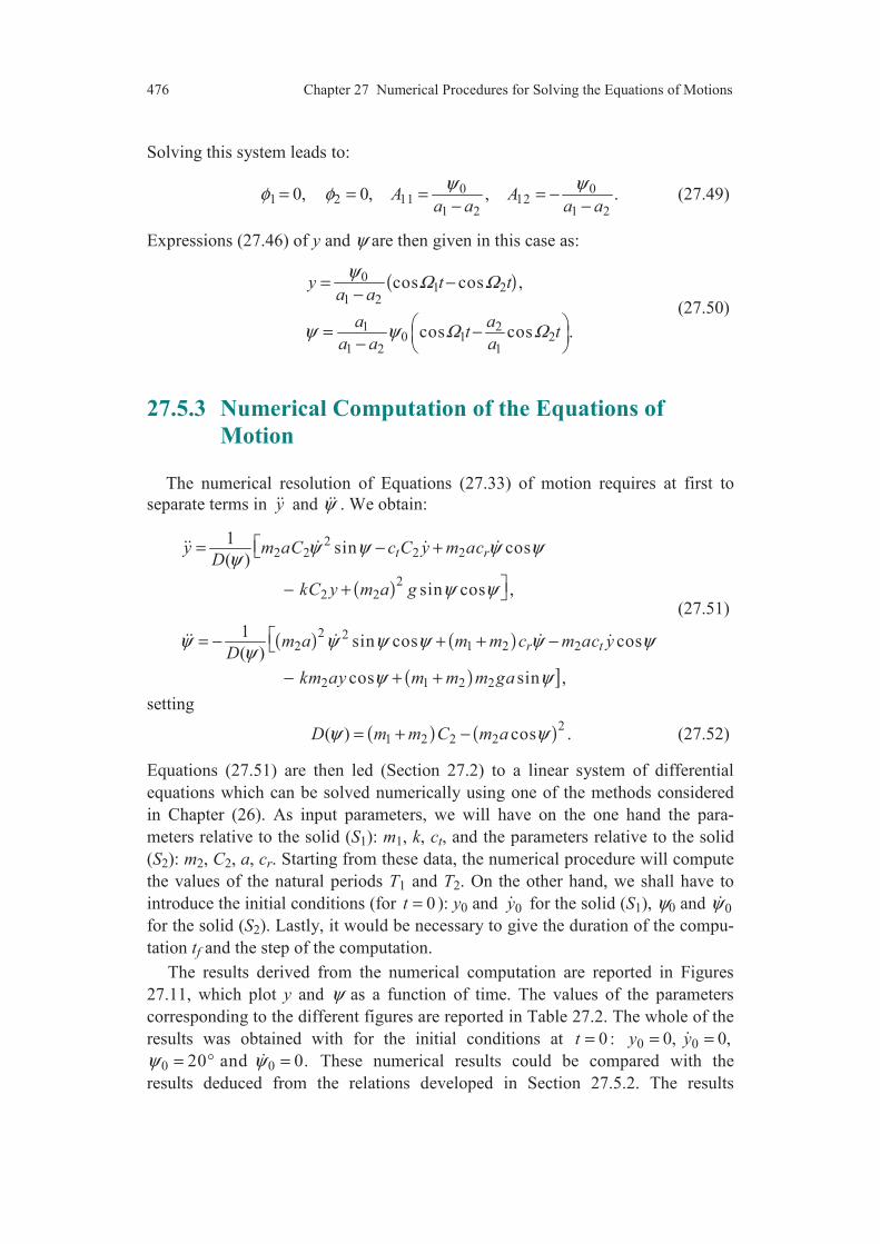
476 Chapter 27 Numerical Procedures for Solving the Equations of Motions
Solving this system leads to:
0 01 2 11 12
1 2 1 2
0, 0, , .A Aa a a a
ψ ψφ φ= = = = −
− − (27.49)
Expressions (27.46) of y and ψ are then given in this case as:
( )01 2
1 2
1 20 1 2
1 2 1
cos cos ,
cos cos .
y t ta a
a at t
a a a
ψΩ Ω
ψ ψ Ω Ω
= −−
= − −
(27.50)
27.5.3 Numerical Computation of the Equations of Motion
The numerical resolution of Equations (27.33) of motion requires at first to
separate terms in y and ψ . We obtain:
( )
( ) ( )
( ) ]
22 2 2 2
22 2
2 22 1 2 2
2 1 2 2
1sin cos
( )
sin cos ,
1sin cos cos
( )
cos sin ,
t r
r t
y m aC c C y m acD
kC y m a g
m a m m c m ac yD
km ay m m m ga
ψ ψ ψ ψψ
ψ ψ
ψ ψ ψ ψ ψ ψψ
ψ ψ
= − +
− +
= − + + −
− + +
(27.51)
setting
( ) ( )21 2 2 2( ) cosD m m C m aψ ψ= + − . (27.52)
Equations (27.51) are then led (Section 27.2) to a linear system of differential
equations which can be solved numerically using one of the methods considered
in Chapter (26). As input parameters, we will have on the one hand the para-
meters relative to the solid (S1): m1, k, ct, and the parameters relative to the solid
(S2): m2, C2, a, cr. Starting from these data, the numerical procedure will compute
the values of the natural periods T1 and T2. On the other hand, we shall have to
introduce the initial conditions (for 0t = ): y0 and 0y for the solid (S1), ψ0 and 0ψfor the solid (S2). Lastly, it would be necessary to give the duration of the compu-
tation tf and the step of the computation.
The results derived from the numerical computation are reported in Figures
27.11, which plot y and ψ as a function of time. The values of the parameters
corresponding to the different figures are reported in Table 27.2. The whole of the
results was obtained with for the initial conditions at 0t = : 0 0,y = 0 0,y =
0 020 and 0.ψ ψ= ° = These numerical results could be compared with the
results deduced from the relations developed in Section 27.5.2. The results

27.5 Coupled Motion of Two Solids 477
TABLE 27.2 Values of the parameters used for deriving the results of Figures 27.11.
Figure 27.11 a b c d e
m1 (kg) 40 20 5 40 5
k (N m–1) 160 80 10 160 10
ct (N m s–1) 0 0 0 0.05 0.05
m2 (kg) 1.5 1.5 1.5 1.5 1.5
C2 (kg m–2) 1.8 1.8 1.8 1.8 1.8
a (m) 0.48 0.48 0.48 0.48 0.48
cr (N m s–1) 0 0 0 0.1 0.1
ω1 (s–1) 2 2 1.4142 2 1.4142
T1 (s) 3.1416 3.1416 4.4429 3.1416 4.4429
ω2 (s–1) 1.9808 1.9808 1.9808 1.9808 1.9808
T2 (s) 3.1720 3.1720 3.1720 3.1720 3.1720
α1 0.9639 0.9302 0.7692 0.9639 0.7692
α2 0.1920 0.1920 0.1920 0.1920 0.1920
α12 0.9931 0.9931 0.9557 0.9931 0.9557
Ω1 (s–1) 2.061 2.0817 2.0535 2.0601 2.0535
Ω2 (s–1) 1.8943 1.8477 1.2237 1.8943 1.2237
a1 – 5.2797 – 4.2202 – 5.7341 – 5.2797 – 5.7341
a2 4.2920 2.6847 0.2470 4.2920 0.2470
tf (s) 80 80 80 160 160
h (s) 0.08 0.08 0.08 0.08 0.08
obtained strongly depend: 1) on the natural periods of each of the two systems, 2)
on the mechanical energies induced in each motion of the solids (S1) and (S2).
According to the values of these energies, there is exchange or not of the energies
induced during the motions of each solid. Beat processes are observed in the case
where the natural frequencies are close (Figures 27.11a, 27.11b and 27.11d),
caused by alternating constructive and destructive interferences.

478 Chapter 27 Numerical Procedures for Solving the Equations of Motions
FIGURE 27.11. Coupled motions of two solids for various values of the parameters.
temps ( s )
0 10 20 30 40 50 60 70 80
rota
tio
n ψ
(
° )
-20
-10
0
10
20
time ( s )
temps ( s )
0 10 20 30 40 50 60 70 80
dép
lace
men
t y
(
m )
-10
-5
0
5
10
dis
pla
cem
ent
y
( m
)
temps ( s )0 10 20 30 40 50 60 70 80
rota
tion
ψ
(
° )
-20
-10
0
10
20
time ( s )
temps ( s )
0 10 20 30 40 50 60 70 80
dép
lace
men
t y
(
m )
-10
-5
0
5
10
time ( s )
dis
pla
cem
ent
y
( m
)
temps ( s )
0 10 20 30 40 50 60 70 80
rota
tion
ψ
(
° )
-20
-10
0
10
20
time ( s )
1
22
2
20 kg,
80 N/m,
0,
1.5 kg,
1.8 kg/m ,
0.48 m,
0.
t
r
m
k
c
m
C
a
c
====
===
1
22
2
5 kg,
10 N/m,
0,
1.5 kg,
1.8 kg/m ,
0.48 m,
0.
t
r
m
k
c
m
C
a
c
====
===
(a)
(b)
(c)
temps ( s )
0 10 20 30 40 50 60 70 80
dép
lace
men
t y
(
m )
-8
-4
0
4
8
time ( s )
dis
pla
cem
ent
y
( m
)
time ( s )
1
22
2
40 kg,
160 N/m,
0,
1.5 kg,
1.8 kg/m ,
0.48 m,
0.
t
r
m
k
c
m
C
a
c
====
===

27.5 Coupled Motion of Two Solids 479
FIGURE 27.11 (continued). Coupled motions of two solids for various values of the
parameters .
EXERCISES 27.1 Implement numerical procedures making it possible to study the various
motions considered in this chapter.
temps ( s )
0 20 40 60 80 100 120 140 160
rota
tion
ψ
(
° )
-20
-10
0
10
20
time ( s )
temps ( s )
0 20 40 60 80 100 120 140 160
dép
lace
men
t y
(
m )
-10
-5
0
5
10
time ( s )
dis
pla
cem
ent
y
( m
)
temps ( s )
0 20 40 60 80 100 120 140 160
rota
tio
n ψ
(
° )
-20
-10
0
10
20
time ( s )
temps ( s )0 20 40 60 80 100 120 140 160
dép
lace
men
t y
(m
)
-6
-4
-2
0
2
4
6d
isp
lace
men
t y
(
m )
time ( s )
1
22
2
40 kg,
160 N/m,
0.05 Nm/s,
1.5 kg,
1.8 kg/m ,
0.48 m,
0.1 Nm/s.
t
r
m
k
c
m
C
a
c
====
===
(d)
1
22
2
5 kg,
10 N/m,
0.05 Nm/s,
1.5 kg,
1.8 kg/m ,
0.48 m,
0.1 Nm/s.
t
r
m
k
c
m
C
a
c
====
===
(e)

480 Chapter 27 Numerical Procedures for Solving the Equations of Motions
COMMENTS
The numerical resolution of the equations of motion of a solid or a
system of solids is particularly important owing to the fact that it is gene-
rally necessary to use it. The reader will pay an extreme attention to the
development of the concepts introduced in the preceding chapter then
applied to the cases of the resolution of the equations of the motions
considered in the present chapter.
So as to implement the procedures for numerically solving the equa-
tions of motion, the reader will endeavour to set up the numerical
procedures which make it possible to analyze the various motions studied
in this chapter. The procedures thus implemented could be then trans-
posed easily to the study of any motion of solids.
Part VII
Solutions of the Exercises
This last part of the textbook reports the solutions of the exercises
proposed all along the chapters of the textbook. The writing has been
developed extensively and structured in such a way to underline the
development of the analyses, and so to improve the capacity of the
comprehension of the reader. The author estimates that a well
structured development of the solutions is indispensable for a good
understanding and a good application of the concepts introduced in
the textbook.


Chapter 1
Vector Space 3
1.1 Let V
be a given vector and u
a vector collinear to this vector.
u
is collinear to V
is expressed as:
, where u Vα α= ∈
.
u
is a unit vector is expressed as:
1u =
.
The two preceding relations lead thus to:
1 ou 1V Vα α= =
.
Hence:
1
Vα = .
Thus, we deduce:
1
Vα = ± .
Hence the expression of the unit vectors:
Vu
V= ±
.
There exist thus two unit vectors collinear to a given vector. They are opposed
and obtained by dividing the vector by its norm.
Numerical application
(2, 5, 3) in the canonical basis.V = −
We have: 38V =
.
Hence: ( )
12 5 3
38u i j k= ± − +
,
or
2 5 3 2 5 3, , and , , .
38 38 38 38 38 38u u
− − − = =
1.2 The necessary and sufficient condition so that the vectors 1V
and 2V
are
orthogonal is that the scalar product is zero. Thus:
1 2 0V V =⋅
or 5 5 0α − = .
Hence: 1α = .
The vector 1V
is thus expressed by 1 (1, 2, 1)V = −
.

484 Chapter 1 Vector Space 3
1.3 Let 1V
and 2V
be the two given vectors. Their vector product 1 2V V V= ×
is
orthogonal to 1V
and to 2 .V
We are brought back to Exercise 1.1. The unit
vectors u
orthogonal to 1V
and to 2V
are thus:
1 2
1 2
V Vu
V V
×= ±
×
.
Numerical application
1 2(2, 5, 3) and ( 2, 1, 3)V V= − = − −
.
Their vector product is: 1 2 12 8V V i k× = −
.
So, the unit vectors are:
( )
112 8
208u i k= ± −
.
1.4 Expansions
1. By applying the distributivity of the scalar product:
( ) ( ) 2 21 2 1 2 1 1 2 2 1 2 .V V V V V V V V V V+ − = − + −⋅ ⋅ ⋅
The scalar product is commutative. Hence:
( ) ( ) 2 21 2 1 2 1 2 .V V V V V V+ − = −⋅
2. Similarly, by applying the distributivity of the vector product:
( ) ( )1 2 1 2 1 1 1 2 2 1 2 2 .V V V V V V V V V V V V+ × − = × − × + × − ×
The vector product of a vector by itself is the null vector and the vector product is
antisymmetric. Hence:
( ) ( ) ( )1 2 1 2 1 22 .V V V V V V+ × − = − ×
1.5 The vector V
has for components (4, –9, 3) in the basis ( )1 1 1(1) , , i j k=
.
Thus:
1 1 14 9 3V i j k= − +
.
The basis (2) is deduced from the basis (1) by the relations:
2 1 2 1 2 12 , 2 , .i i j j k k= = = −
Hence by substituting into the expression of V
:
2 2 29
2 32
V i j k= − −
.
In the basis (2), the components of V
are thus (2, –3.5, –3).
1.6 We have to derive the vectors V
such that: 1 2 1V V V V× = ×
, where 1V
and
2V
are two given vectors.

Solution of Exercise 1.6 485
We have to proceed by equivalences starting from the given relation. While
passing the first member of the equation into the second one, we have:
1 1 2 0V V V V× − × =
.
Considering the distributivity, it comes:
( )1 2 0V V V× − =
.
The necessary and sufficient condition so that the vector product of the vectors 1V
and 2V V−
is null is that these vectors are collinear. For example:
2 1, V V Vα α− = ∀ ∈
.
Hence the expression of the vector:
2 1, V V Vα α= + ∀ ∈
.
Numerical application
1 24 and 5 6 2V i j V i j k= − = + −
.
The result is:
( ) ( ) 5 6 4 2 , V i j kα α α= + + − − ∀ ∈
.

Chapter 2
The Geometric Space
2.1 We express that the point H is the orthogonal projection of the point M on
the line (D) (Figure 2.16).
The point H is the orthogonal projection of the point M. Hence MH is
orthogonal to the line (D). Thus:
0HM V =⋅
.
The point M is a point of (D):
, OH Vα α= ∈
.
To derive the position of the point H, we have to obtain the expression of its
position vector as a function of the data of the problem: direction vector V
and
position vector OM
of the point M.
The first relation is written:
( ) 0 or 0OM OH V OM V OH V− = − =⋅ ⋅ ⋅
.
Hence by introducing the expression of OH
, we have:
20OM V Vα− =⋅
.
Hence the expression of α :
2
OM V
Vα =
⋅
,
and the expression of the position vector OH
:
2
OM VOH V
V=
⋅
.
If the vector V
is the unit direction vector u
of the line (D): 2 1u =
, the
expression of OH
is reduced to:
( )OH OM u u= ⋅
.
Numerical application
The vector V
has for components (1, −2, 3) and the position vector OM
has
for components (x, y, z), the coordinates of the point M. Hence:
214 and 2 3V OM V x y z= = − +⋅
.
The coordinates ( , , )H H Hx y z of the point H are thus:
1 1 3( 2 3 ), ( 2 3 ), ( 2 3 ).
14 7 14H H Hx x y z y x y z z x y z= − + = − + − = − +

Solution of Exercise 2.2 487
2.2 Straight line passing through the point A and orthogonal to the plane passing
through the points A, B and C.
The line may be defined by ( ), A u
where u
is the unit vector of the direction
orthogonal to the plane (A, B, C).
Two direction vectors of the plane are given by AB
and AC
image vectors of
the respective bipoints (A, B) and (A, C). An orthogonal vector is given by
AB AC×
. The vector u
is a unit vector collinear to the vector product AB AC×
.
We are thus brought back to Exercice 1.1. Hence:
AB ACu
AB AC
×=
×
,
taking the + determination of the vector.
Numerical application
A (–1, 2, 1), B (2, 3, –1), C (–3, 4, –2).
Hence:
AB =
(3, 1, –2), AC =
(–2, 2, –3),
and
( ) + 1, 13, 8 , + 234AB AC AB AC= =
.
The vector u
is thus:
1 13 8
234 234 234u i j k= + +
.
It is then easy to find the Cartesian equations of the line.
2.3 So that the triangle ABC is isosceles and right-angled at A, we have to show
that the edges AB and AC are equal and are orthogonal. Or:
? ? .and 0AB ACAB AC == ⋅
Derivation of the vectors AB
and AC
:
( ) ( )1 2, 2, 1 2 , 1 2, 2, 1 2 .AB AC= − + = − − − − +
Orthogonality:
( )( ) ( )( )1 2 1 2 2 1 2 1 2 .AB AC = − − − − + + − +⋅
Hence: 0.AB AC =⋅
The triangle is thus right-angled at A.
Equality of the edges:
( ) ( )
( ) ( )
2 2
2 2
1 2 2 1 2 ,
1 2 2 1 2 .
AB AB
AC AC
= = − + + +
= = − − + + − +
Thus: AB AC=
.
The two edges of the triangle are equal. So it is isosceles and right-angled at A.
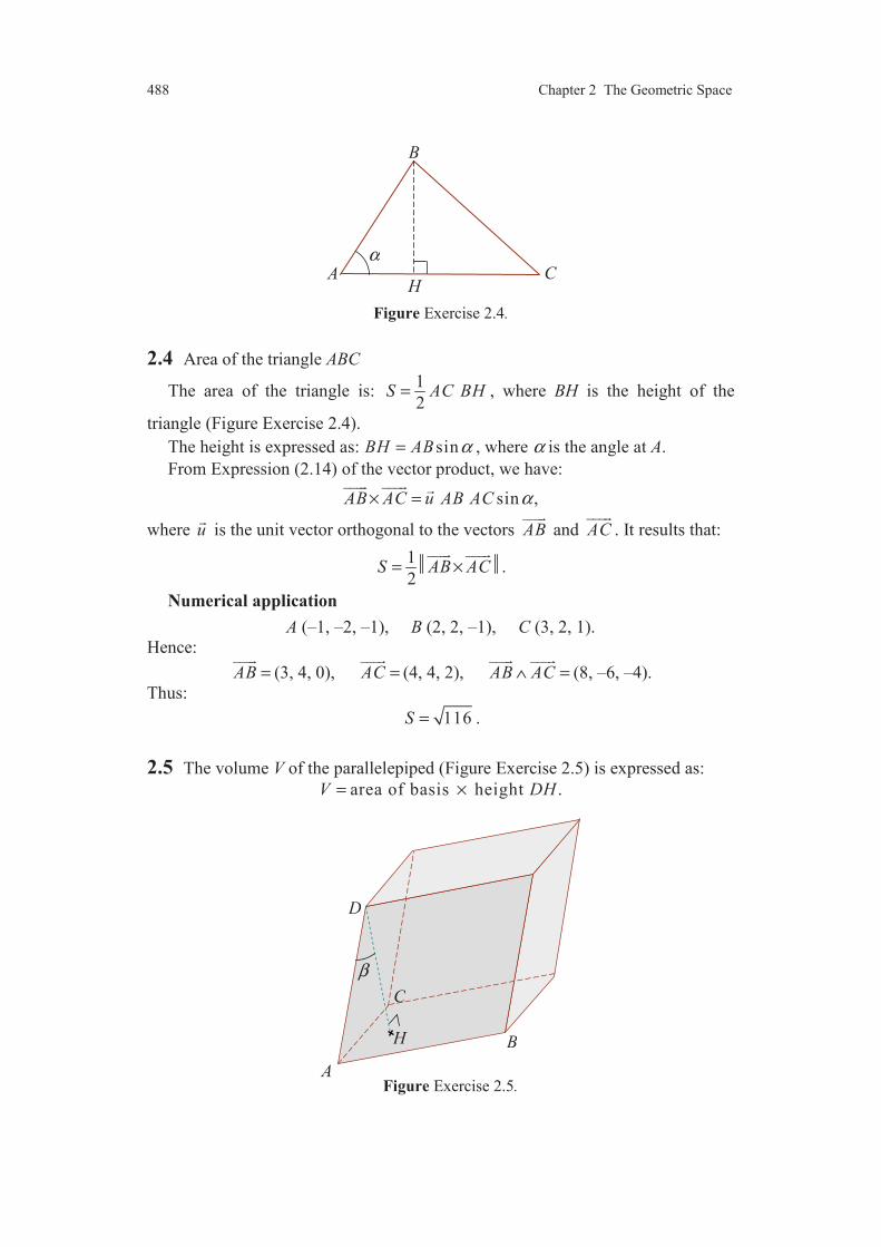
488 Chapter 2 The Geometric Space
Figure Exercise 2.4.
2.4 Area of the triangle ABC
The area of the triangle is: 1
2S AC BH= , where BH is the height of the
triangle (Figure Exercise 2.4).
The height is expressed as: sinBH AB α= , where α is the angle at A.
From Expression (2.14) of the vector product, we have:
sin ,AB AC u AB AC α× =
where u
is the unit vector orthogonal to the vectors AB
and AC
. It results that:
1
2S AB AC= ×
.
Numerical application
A (–1, –2, –1), B (2, 2, –1), C (3, 2, 1).
Hence:
AB =
(3, 4, 0), AC =
(4, 4, 2), AB AC∧ =
(8, –6, –4).
Thus:
116S = .
2.5 The volume V of the parallelepiped (Figure Exercise 2.5) is expressed as:
area of basis height .V DH= ×
Figure Exercise 2.5.
A
B
C H
α
A
B
C
D
H
β

Solution Exercise 2.5 489
From the preceding exercise, the area of the basis is: S AB AC= ×
.
The height is expressed by cosDH AD β= , where β is the angle between the
bipoints (D, A) and (D, H). Hence the expression of the volume:
cosV AB AC AD β= ×
.
Thus, from the expression (2.13) of the scalar product:
( ) V AB AC AD= × ⋅
.
The volume of the parallelepiped is thus equal to the mixed product of the
vectors images of the bipoints on which the parallelepiped is constructed.
Numerical application
A (0, 0, 0), B (3, 2, 1), C (1, 1, 2), D (−1, −1, 2).
Hence:
AB =
(3, 2, 1), AC =
(1, 1, 2), AD =
(−1, −1, 2),
AB AC× =
(3, −5, 1), ( ) 4AB AC AD× =⋅
.
Hence the volume: 4V = .
2.6 The distance d from the point D to the plane passing through the three points
A, B and C is the height of the parallelepiped constructed on the bipoints (A, B),
(A, C) and (A, D). The results of the preceding exercises lead to:
( )
volume
area of basis
AB AC ADd
AB AC
×= =
×
⋅
.
Numerical application
A (0, 0, 0), B (1, 2, 3), C (2, 1, 1), D (−2, −1, −3).
Hence:
AB =
(1, 2, 3), AC =
(2, 1, 1), AD =
(−2, −1, −3),
AB AC× =
(−1, 5, −3), 35AB AC× =
, ( ) 6AB AC AD× =⋅
.
The distance is thus: 6
35d = .
2.7 The necessary and sufficient condition so that the four points A, B, C and D
are contained in the same plane is that the point D is contained in the plane
passing trough the points A, B and C. Thus, the distance from the point D to the
plane is zero. From the preceding exercise, the condition is:
( ) 0AB AC AD× =⋅
.
2.8 The two rotations considered are reported in Figure Exercise 2.8.
2.8.1. First rotation
( ) 1 1 1/ , ,O i j k
( ) 1 3 2/ , ,O i j k
. ( )1, 30i °

490 Chapter 2 The Geometric Space
Figure Exercise 2.8.
The basis change is written:
1
3 1 1
2 1 1
,
cos30 sin 30 ,
sin 30 cos30 ,
i
j j k
k j k
= ° + ° = − ° + °
or
1
3 1 1
2 1 1
,
3 1 ,2 2
31 .2 2
i
j j k
k j k
= + = − +
Second rotation
( ) 1 3 2/ , ,O i j k
( ) 2 2 2/ , ,O i j k
.
The basis change is written:
2 1 3
2 1 3
2
cos 45 sin 45 ,
sin 45 cos 45 ,
,
i i j
j i j
k
= ° + °
= − ° + °
or
2 1 3
2 1 3
2
2 2 ,2 2
2 2 ,2 2
.
i i j
j i j
k
= +
= − +
z1
x1
O
1i
y1
y3
2k
x2
z2y2
2i 1j3j
2j
1k
45°
45°
30°
30°
45°
30°
( )2 , 45k °
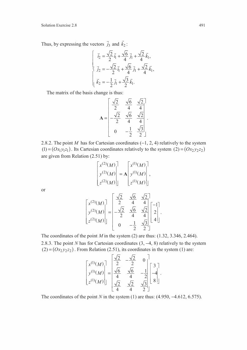
Solution Exercise 2.8 491
Thus, by expressing the vectors 3j
and 2k
:
2 1 1 1
2 1 1 1
2 1 1
62 2 ,2 4 4
62 2 ,2 4 4
31 .2 2
i i j k
j i j k
k j k
= + +
= − + +
= − +
The matrix of the basis change is thus:
2 6 2
2 4 4
2 6 2
2 4 4
1 30
2 2
= − −
A .
2.8.2. The point M has for Cartesian coordinates (−1, 2, 4) relatively to the system
( )1 1 1(1) Ox y z= . Its Cartesian coordinates relatively to the system ( )2 2 2(2) Ox y z=
are given from Relation (2.51) by:
( )
( )
( )
( )
( )
( )
(2) (1)
(2) (1)
(2) (1)
x M x M
y M y M
z M z M
=
A ,
or
( )
( )
( )
(2)
(2)
(2)
62 22 4 4 1
62 2 22 4 4
4310
2 2
x M
y M
z M
− = − −
.
The coordinates of the point M in the system (2) are thus: (1.32, 3.346, 2.464).
2.8.3. The point N has for Cartesian coordinates (3, −4, 8) relatively to the system
( )2 2 2(2) Ox y z= . From Relation (2.51), its coordinates in the system (1) are:
( )
( )
( )
(1)
(1)
(1)
2 2 02 2 36 6 1 4
4 4 28
32 24 4 2
x M
y M
z M
− = − −
.
The coordinates of the point N in the system (1) are thus: (4.950, −4.612, 6.575).
Chapter 4
Elementary Concepts on Curves
4.1 The position vector of a point M of the curve (C) is expressed by:
( )3 3sin cos cos 2OM a i q j q k q= + −
,
with 0a > and 02
qπ
< < .
4.1.1. Unit direction vector of the tangent
A direction vector V
of the tangent is obtained by deriving the position vector
OM
with respect to the parameter q. Thus:
( )2 2d3 sin cos 3 cos sin 2 sin 2
d
OMV a i q q j q q k q
q= = − −
,
or
( )dsin cos 3 sin 3 cos 4
d
OMV a q q i q j q k
q= = − −
.
From Exercise 1.1, the unit vector te
of the tangent is given by:
tV
eV
= ±
,
with
2 2sin cos 9sin 9cos 16 5 sin cosV a q q q q a q q= + + =
.
Hence:
( )13 sin 3 cos 4
5te i q j q k= ± − −
.
Hereafter, we shall take the + determination which orientates the curve in the
direction of increasing q.
4.1.2. Curvilinear abscissa
The curvilinear abscissa s can be introduced while writing:
d d d
d d d
OM OM s
q s q=
.
Thus from (4.9):
d d
d dt
OM se
q q=
.
The expressions of d
d
OM
q
and te
obtained previously lead then:
d5 sin cos
d
sa q q
q= ,
or integrating:

Solution Exercise 4.1 493
0
0( ) ( ) 5 sin cos dq
q
s q s q a q q q− = .
The integration leads to:
( )2 20 0
5( ) ( ) sin sin
2s q s q a q q− = − .
By taking as the origin of the curvilinear abscissae the point M0 where the point
point M is located when 0( ) 0,s q = the curvilinear abscissa is given by:
25( ) sin
2s q a q= .
4.1.3. Unit vector of the principal normal direction and radius of curvature
They are expressed by Relation (4.11), with here:
( )d d d 1 13 cos 3 sin
d d d 5 5 sin cost te e q
i q j qs q s a q q
= = +
.
Hence:
( )3cos sin
25 sin cosne
i q j qa q q
= +
.
Thus, we deduce:
cos sin ,
25sin cos .
3
ne i q j q
a q q
= +
=
The vector ne
and the radius of curvature were already separated.
4.1.4. Frenet basis The third vector of the Frenet basis is obtained by Relation (4.12). Thus:
( ) ( )13 sin 3 cos 4 cos sin
5be i q j q k i q j q= − − × +
.
That leads to:
( )14 sin 4 cos 3
5be i q j q k= − +
.

Chapter 5
Torsors
5.1 Let ( ) D be the torsor associated to the field of sliders defined on the
domain (D) constituted of the four points M1, M2, M3 and M4.
5.1.1. Resultant of the torsor ( ) R D
( ) 4
1
i
i
R D R
=
= .
Thus:
( ) 8 2 4R D i j k= + +
.
5.1.2. Moment of the torsor at the point OGenerally the calculation of the moment is easier at the origin of the coor-
dinates. Thus:
( ) 4
1
iiO
i
D OM R
=
= × ,
with
11
22
33
44
15 10 ,
2 8 ,
6 15 ,
2 6 .
OM R j k
OM R i k
OM R i j
OM R i k
× = +
× = − +
× = − −
× = −
Hence:
( ) 6 12O D i k= − +
.
5.1.3. Caracterization of the torsorThe scalar invariant of the torsor is:
( ) ( ) ( ) OI D R D D= ⋅
.
Calculation leads to ( ) 0I D = . The resultant being different from the null
vector, the torsor is a slider.
5.1.4. Moment of the torsor at a point PThe point P has for coordinates (x, y, z) relatively to the system (Oxyz). Hence:
OP x i y j z k= + +
.
The moment at the point P is given by:
( ) ( ) ( ) P OD D R D OP= + × ,
with
( ) ( ) ( ) ( )2 4 4 8 8 2R D OP z y i x z j y x k× = − + − + −
.
Hence:
( ) ( ) ( ) ( )2 2 3 4 2 2 4 6P D y z i x z j x y k= − + − + − + − + −
.
Solution Exercise 5.1 495
5.1.5. Axis of the torsorThe torsor being a slider, it has an axis of null moments, set of the points at
which the moment of the torsor is null. Thus, the set of the points P such as:
( ) 0P D = .
That leads to
2 3 0,
2 0,
4 6 0.
y z
x z
x y
− + − =
− =
− + − =
A straight line is defined by two equations. Among the three preceding equations,
one of the equations is a linear combination of the two others. For example, the
equations of the axis will be:
2 3 0,
2 0.
y z
x z
− + − =
− =
The axis can be determined by two points A and B. For example the point A for
which 0x = and the point B for which 0y = . We obtain:
A (0, 32
− , 0) and B (6, 0, 3).
The axis can also be defined by a point (A for example) and a direction vector:
the resultant of the torsor 8 2 4i j k+ +
.
5.2 On the same domain (D) as the preceding exercise, it is defined a new field
of sliders. And let ( ) D be the torsor associated to this new field.
5.2.1. Resultant of the torsor ( ) R D
( ) 4
1
i
i
R D R
=
= .
Thus:
( ) 0R D = .
5.2.2. Moment of the torsor at the point O
( ) 4
1
iiO
i
D OM R
=
= × ,
with
11
22
33
44
300 200 ,
100 200 800 ,
100 50 200 ,
0.
OM R j k
OM R i j k
OM R i j k
OM R
× = +
× = − + −
× = − −
× =
Thus:
( ) 450 800O D j k= −
.

496 Chapter 5 Torsors
5.2.3. Caracterization of the torsor The torsor having a null resultant and a non null moment is a couple-torsor. Its
moment is independent of the point:
( ) 450 800 , P D j k P= − ∀
.
5.2.4. Resolution of the couple-torsor at the point O
The couple-torsor ( ) D can be resolved into two sliders ( ) 1 D and
( ) 2 D . Thus:
( ) ( ) ( ) 1 2D D D= + .
The resolution being implemented at the point O, we have:
( ) ( ) ( )
( ) ( ) ( ) 1 2
1 2
,
.O O O
R D R D R D
D D D
= +
= +
We choose the slider ( ) 1 D so that its axis passes through the point O. Thus:
( ) 1 0O D = .
Hence the elements of reduction at the point O of the slider ( ) 2 D :
( ) ( )
( ) ( )
2 1
2
,
450 800 .O O
R D R D
D D j k
= −
= = −
The sliders are then completely determined by choosing a resultant for one of the
sliders.
5.3 Let ( ) D be the new torsor associated to the field of sliders defined on
the domain (D).
5.3.1. Resultant
( ) 8 2 5R D i j k= − +
.
5.3.2. Moment at the point O
11
22
33
44
10 13 2 ,
2 8 ,
6 15 ,
2 6 .
OM R i j k
OM R i k
OM R i j
OM R i k
× = + +
× = − +
× = − −
× = −
Hence:
( ) 4 2 4O D i j k= − +
.
5.3.3. Caracterization of the torsor The scalar invariant of the torsor is:
( ) ( ) ( ) 56OI D R D D= =⋅
.

Solution Exercise 5.3 497
The scalar invariant is different from zero. Thus it results that the torsor is arbi-
trary.
5.3.4. Moment at a point P of coordinates ( ), , x y z
( ) ( ) ( ) P OD D R D OP= + × ,
with
( ) ( ) ( ) ( )2 5 5 8 8 2R D OP z y i x z j y x k× = − − + − + +
.
Hence:
( ) ( ) ( ) ( )5 2 4 5 8 2 2 8 4P D y z i x z j x y k= − − + + − − + + +
.
5.3.5. Central axis of the torsor It is the set of the points P such as the moment of the torsor at the point P is
collinear to the resultant:
( ) ( ) , P D R Dα α= ∀ ∈
.
That leads to:
5 2 4 8 ,
5 8 2 2 ,
2 8 4 4 .
y z
x z
x y
α
α
α
− − + =
− − = −
+ + =
The equations of the axis are obtained by eliminating α. Thus:
20 5 34 4 0,
12 8 16 2 0.
x y z
x y z
− − − =
+ − + =
The axis can be eventually defined by two points of coordinates deduced from the
preceding equations.
5.3.6. Resolution of the torsor at the point O
The arbitrary torsor ( ) D is resolved into a slider ( ) 1 D and a couple-
torsor ( ) 2 D . Thus:
( ) ( ) ( ) 1 2D D D= + .
The resolution being implemented at the point O, we have:
( ) ( ) ( )
( ) ( ) ( ) 1 2
1 2
,
.O O O
R D R D R D
D D D
= +
= +
The couple-torsor is such as ( ) 2 0R D = and the slider is chosen so that its axis
of null moments passes through the point O. It results that the slider has for
elements of reduction:
( ) ( )
( )
1
1
8 2 5 ,
0,O
R D R D i j k
D
= = − +
=
and the couple-torsor is such as:

498 Chapter 5 Torsors
( )
( ) ( )
2
2
0 ,
4 2 4 , .P O
R D
D D i j k P
=
= = − + ∀
Solution Exercise 5.3 499
5.4 We consider then the domain (D) constituted of a rectangular area. To every
area element surrounding the point M it is associated a slider of vector density
( )p M i
:
( )M D∀ ∈ slider of resultant d ( ) ( ) d ( )R M p M i S M=
and of axis ( ), M i
.
Let ( ) D be the torsor associated to this field of sliders.
5.4.1. Resultant The resultant is expressed by:
( ) ( )
d ( )D
R D R M= .
Considering the Cartesian coordinates, the area element surrounding the point M
is an elementary rectangle of edges d and dx y : d ( ) d dS M x y= . The resultant is
then expressed as:
( )
0 0
( )d da b
x y
R D i p M x y= =
= ,
where a and b are the respective edges of the rectangle. The integral depends on
the expression of ( )p M .
In the case of a constant function for ( )p M : 0( )p M p= , the resultant is
simply expressed as:
( ) 0R D p S i= ,
where S is the area of the rectangle: S ab= .
5.4.2. Moment of the torsorThe moment of the torsor is determined while expressing this moment at a
point. It is also possible to search for a point where the moment is known. We are
here in the important particular case considered in Subsection 5.3.3: the resultant
of the slider associated to the element surrounding the point M is a vector whose
the direction i
is independent of the point M. In this case there exists a measure
centre H and the moment at this point is null. By searching this point H, we
answer in search for the moment of the torsor since:
( ) 0H D = .
Furthermore in this case, the resultant is expressed (5.66) as:
( ) ( )R D D iµ= ,
where ( )Dµ is the measure of the domain (D), associated to the field of sliders
under consideration:
0 0
( ) ( ) d da b
x y
D p M x yµ= =
= .
If ( )p M is constant over the domain (D), we have:
0( )D p Sµ = .

500 Chapter 5 Torsors
The position of the point H is given by Expression (5.72). That leads here to:
( )
0 0
1( ) d d
( )
a b
x y
OH x i y j p M x yDµ = =
= +
.
The coordinates ( ), , 0H Hx y of the point H are then deduced from this expres-
sion and are expressed as:
0 0
0 0
1( ) d d ,
( )
1( ) d d .
( )
a b
Hx y
a b
Hx y
x x p M x yD
y y p M x yD
µ
µ
= =
= =
=
=
If p(M) is constant over the domain (D):
0 0
0 0
1d d ,
1d d .
a b
Hx y
a b
Hx y
x x x yS
y y x yS
= =
= =
=
=
The point H coincides with the centre of the rectangle.
Having obtained the position of the measure centre H, it is then possible to
derive the moment at an arbitrary point using the expression:
( ) ( ) P D R D HP= × .
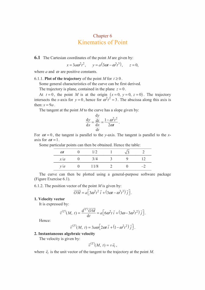
Chapter 6
Kinematics of Point
6.1 The Cartesian coordinates of the point M are given by:
( )2 2 3 33 , 3 , 0,x a t y a t t zω ω ω= = − =
where a and ω are positive constants.
6.1.1. Plot of the trajectory of the point M for 0t ≥ .
Some general characteristics of the curve can be first derived.
The trajectory is plane, contained in the plane 0z = .
At 0t = , the point M is at the origin ( )0, 0, 0x y z= = = . The trajectory
intersects the x-axis for 0y = , hence for 2 2 3tω = . The abscissa along this axis is
then: 9x a= .
The tangent at the point M to the curve has a slope given by:
2 2d
d 1ddd 2
d
yy tt
xx t
t
ωω
−= = .
For 0tω = , the tangent is parallel to the y-axis. The tangent is parallel to the x-
axis for 1tω = .
Some particular points can then be obtained. Hence the table:
tω 0 1/2 1 3 2
/x a 0 3/4 3 9 12
/y a 0 11/8 2 0 –2
The curve can then be plotted using a general-purpose software package
(Figure Exercise 6.1).
6.1.2. The position vector of the point M is given by:
( )2 2 3 33 3OM a t i t t jω ω ω = + −
.
1. Velocity vector It is expressed by:
( )( )
( )2 3 2d( , ) 6 3 3
d
TT OM
M t a t i t jt
ω ω ω = = + −
.
Hence: ( ) ( )2 2( , ) 3 2 1T M t a t i t jω ω ω = + −
.
2. Instantaneous algebraic velocity The velocity is given by:
( )( , )T
tM t e= ,
where te
is the unit vector of the tangent to the trajectory at the point M.
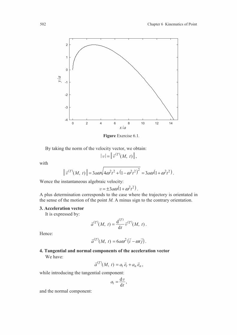
502 Chapter 6 Kinematics of Point
0 2 4 6 8 10 12 14-4
-3
-2
-1
0
1
2
/x a
/y
a
Figure Exercise 6.1.
By taking the norm of the velocity vector, we obtain: ( )
( , )T M t=
,
with
( ) ( ) ( )22 2 2 2 2 2( , ) 3 4 1 3 1T M t a t t a tω ω ω ω ω= + − = + .
Wence the instantaneous algebraic velocity:
( )2 23 1a tω ω= ± + .
A plus determination corresponds to the case where the trajectory is orientated in
the sense of the motion of the point M. A minus sign to the contrary orientation.
3. Acceleration vector It is expressed by:
( )( )
( )
d( , ) ( , )
d
TT Ta M t M t
t=
.
Hence: ( ) ( )2( , ) 6Ta M t a i t jω ω= −
.
4. Tangential and normal components of the acceleration vector We have:
( ) ( , )T
t t n na M t a e a e= +
,
while introducing the tangential component:
d
dta
t=
,
and the normal component:

Solution Exercise 6.1 503
2
na =
,
where is the radius of curvature of the trajectory at the point M.
The tangential component is then:
36ta a tω= .
The radius of curvature being not known, it is not possible to deduce the normal
component from the previous expression. So, we use the expression of the accele-
ration vector while expressing its norm:
( )
2 2( , )Tt na M t a a= +
.
Thus:
( )2 4 2 2 2 6 2 236 1 36 na t a t aω ω ω+ = + or 2 2 436na a ω= .
Hence:
26na aω= ± .
The component an being positive, we deduce then:
26na aω= .
5. Radius of curvature
It is expressed by: 2
na=
.
Hence: ( )22 231
2a tω= + .
6. Curvilinear abscissa The curvilinear abscissa at time t can be derived from the expression of the
instantaneous algebraic velocity:
d
d
s
t= .
Thus integrating between the instants t0 and t:
( )
0 0
2 20( ) ( ) d 3 1 d
t t
t t
s t s t t a t tω ω− = = + .
We obtain:
( ) ( )2
3 30 0 0( ) ( ) 3
3s t s t a t t t t
ωω
− = − + − .
Taking the origin of the curvilinear abscissae for 0t = ( 0( 0) 0s t = = ), we have:
2 2
( ) 3 13
ts t a t
ωω
= +
.
6.2 A cyclist, a car and a truck move between the cities A and B distant of 160
km (Figure Exercise 6.2).
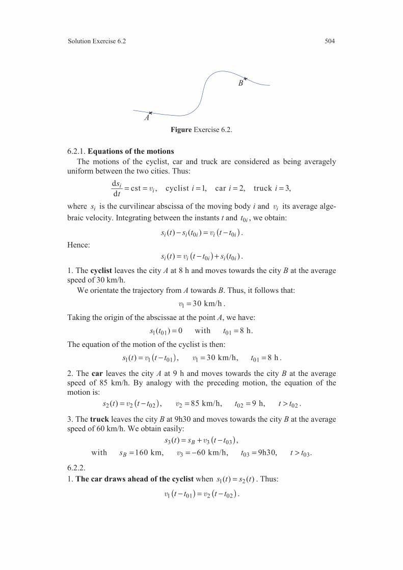
Solution Exercise 6.2 504
Figure Exercise 6.2.
6.2.1. Equations of the motionsThe motions of the cyclist, car and truck are considered as being averagely
uniform between the two cities. Thus:
dcst , cyclist 1, car 2, truck 3,
di
is
i i it
= = = = =
where is is the curvilinear abscissa of the moving body i and i its average alge-
braic velocity. Integrating between the instants t and 0it , we obtain:
( )0 0( ) ( )i i i i is t s t t t− = − .
Hence:
( )0 0( ) ( )i i i i is t t t s t= − + .
1. The cyclist leaves the city A at 8 h and moves towards the city B at the average
speed of 30 km/h.
We orientate the trajectory from A towards B. Thus, it follows that:
1 30 km/h= .
Taking the origin of the abscissae at the point A, we have:
1 01 01( ) 0 with 8 h.s t t= =
The equation of the motion of the cyclist is then:
( )1 1 01 1 01( ) , 30 km/h, 8 hs t t t t= − = = .
2. The car leaves the city A at 9 h and moves towards the city B at the average
speed of 85 km/h. By analogy with the preceding motion, the equation of the
motion is:
( )2 2 02 2 02 02( ) , 85 km/h, 9 h, s t t t t t t= − = = > .
3. The truck leaves the city B at 9h30 and moves towards the city B at the average
speed of 60 km/h. We obtain easily:
( )3 3 03
3 03 03
( ) ,
with 160 km, 60 km/h, 9h30, .
B
B
s t s t t
s t t t
= + −
= = − = >
6.2.2.
1. The car draws ahead of the cyclist when 1 2( ) ( )s t s t= . Thus:
( ) ( )1 01 2 02t t t t− = − .
A
B
Solution Exercise 6.2 505
Hence:
2 02 1 01
2 1
t tt
−=
−
.
We obtain: 9h32min 44st = .
The place where the car passes the cyclist is given by:
2 02 1 011 1 01
2 1
( )t t
s s t t− = = − −
.
Thus: 46.364 kms = .
2. The truck meats the cyclist when 3 1( ) ( )s t s t= . Hence:
( ) ( )3 03 1 01Bs t t t t+ − = − .
Hence:
3 03 1 01
1 3
Bs t tt
− +=
−
.
We obtain: 10h46min 40st = .
The place of the meeting is given by:
3 03 1 011 1 01
1 3
( ) Bs t ts s t t
− + = = − −
.
Hence: 83.333 kms = .
3. The truck meets the car when 3 2( ) ( )s t s t= . By analogy with the preceding
results, we have:
3 03 2 02
2 3
Bs t tt
− +=
−
,
3 03 2 022 2 02
2 3
( ) Bs t ts s t t
− + = = − −
.
Hence at the time 10h18min 37st = , at the distance 111.379 km from the city A.
Chapter 7
Study of Particular Motions
7.1 Performances of a car7.1.1. The performances are established on a car-track of high radius of curvature
and the different stages of the motions are considered as being, on average,
uniformly accelerated. From Section 7.1.3, the equation of the different stages of
the motions can be written in the form:
( ) ( )200 0 0 0
2
as t t t t s= − + − + ,
The car starting at 0t from the position 0s with the velocity 0 , and where 0a is
the average acceleration. The velocity is given by:
( )0 0 0a t t= − + .
Initial accelerations The car starts at time 0 0t = , from the position 0 0s = with a velocity 0 0= .
The equation of the motion is:
20
1
2s a t= ,
and the velocity is:
0a t= .
This latest relation allows us to determine the average acceleration 0a , then to
obtain the distance s covered during the acceleration:
01
, 2
a s t= =
,
where t is the duration of the acceleration and the velocity reached at the end of
the acceleration.
Acceleration stages The car passes at the time 0 0t = at the position 0 0s = while accelerating from
the velocity 0 . The equation of the motion is thus:
20 0
1
2s a t t= + ,
and the velocity is:
0 0a t= + .
This expression allows us to obtain the average acceleration 0a , then the distance
s covered during the acceleration:
( )00 0
1,
2a s t
−= = +
,
where t is the duration of the acceleration and the velocities 0 and at the
beginning and at the end of the acceleration are known.

Solution Exercise 6.1 507
The results obtained for the initial accelerations and the acceleration stages are
reported in the following table.
Table of the accelerations
time
(s)
average
acceleration a0
(m/s2)
covered
distance s
(m)
Initial accelerations
0 to 60 km/h 6.4 2.60 53.3
0 to 80 km/h 10.5 2.12 116.7
Acceleration stages
30 to 100 km/h in 4th 21.6 0.900 390.0
in 5th 30.0 0.648 541.7
40 to 100 km/h in 4th 18.7 0.891 363.6
in 5th 26.4 0.631 513.3
80 to 100 km/h in 3rd 5.7 0.974 142.5
in 4th 6.9 0.805 172.5
in 5th 9.5 0.585 237.5
80 to 120 km/h in 4th 14.6 0.761 405.6
in 5th 18.4 0.604 511.1
7.1.2. Succession of stages:
a. acceleration from 0 to 80 km/h: time 10.5 s and covered distance 116.7 m;
b. 80 to 100 km/h in 3rd: time 5.7 s and covered distance 142.5 m;
c. 100 to 120 km/h in 4th: average acceleration 20 0.761 m/sa = ;
d. beyond 120 km/h in 5th: average acceleration 20 0.604 m/sa = .
7.1.2.1. Time and distance necessary to reach the speed of 100 km/h
This acceleration phase corresponds to the stage a followed by the stage b.
Thus, the time is 12.6 s and the distance is 259.2 m.
Time and distance necessary to reach the speed of 120 km/h: stages a, b and c.
For the stage c, we have: 0 0a t= + , and the duration of the stage c is:
0
0
ta
−=
,
with 20 0.761 m/sa = , 0 100 km/h= and 120 km/h= . Hence:
stage c 7.3 st = ,
and the covered distance is given by:
( ) ( ) 00 0
0
1 1
2 2s t
a
−= + = +
.
Hence:
stage c 223.1 mx = .
Thus, the time and the distance necessary to reach 120 km/h are respectively:
23.5 s and 482.3 m.

Solution Exercise 7.2 508
7.1.2.2. Time and speed reached after 1 000 m
To the stages a, b and c, we have to add the stage with an average acceleration
0a = 20.604 m/s . Taking the origin of times and distances at the beginning of
the stage d, the equation of the motion is:
20 0
1
2s a t t= + .
The distance which remains to be covered is 517.7 m. The duration t of the stage d
is thus solution of:
2 1200.302 517.7 0
3.6t t+ − = .
Solving this equation leads to 13.8 st = .
The time necessary to cover the distance of 1,000 m is thus 37.3 s.
The velocity reached is given by 0 0a t= + , that leads to 150.007 km/h.
7.2 The coordinates of the point M are expressed (7.51) by:
200 00, cos , sin .
2
ax y t z t tϕ ϕ= = = −
7.2.1. If 2
πϕ = , the trajectory is a straight line which reaches a maximum along z:
20
max02
za
=
.
If 2
πϕ ≠ , the trajectory of the point M is:
( )2 2020
1 tan tan2
az y yϕ ϕ= − + +
.
For a given value of the initial velocity 0 , the trajectories depend on the parameter
tanϕ .
So that a point P of the plane (Oxyz) can be a position of the point M, it is
necessary that its coordinates yP and zP satisfy the inequality:
20 02
0022
P Pa
z ya
≤ − +
.
Thus, the point P has to be located inside the parabola of equation:
2 420 0 0 0
2 2 200 0 0
22 2
a az y y
a a
= − + = − −
.
This parabola is envelope of the parabolic trajectories when tanϕ varies. This
envelope has for axis the axis Oz
, its maximum along this axis is 20
02a
and this

Solution Exercise 7.2 509
envelope is reached by the trajectory at the point of coordinate20
0 tanz
a ϕ=
.
7.2.2. Any point Q inside this envelope has its coordinates related by:
( )2
0 2
20
1 tan tan2
QQ Q
a yz yϕ ϕ= − + +
,
where the coordinates yQ and yQ are given. This equation has two roots and these
roots determine the angles 1ϕ and 2ϕ for which it is possible to reach the point Q.
If the point Q is located along the axis Oy
( 0)Qz = , the preceding equation is
written:
( )2
0 2
20
1 tan tan 02
a yyϕ ϕ− + + =
,
or 2 2
0 02
2 20 0
tan tan 02 2
Q QQ
a y a yyϕ ϕ− + =
.
This equation has two roots 1tanϕ and 2tanϕ , such as:
1 2tan tan 1ϕ ϕ = .
The angles 1ϕ and 2ϕ are thus related by:
1 22
πϕ ϕ+ = .
To reach a given horizontal point, there exist thus two shoot angles, a low angle
and a high angle. These two angles differ from 90°.

Chapter 9
Kinematics of Rigid Body
9.1 Motion of a parallelepiped on a plane (Figure 9.10)
The analysis of the kinematics of a solid is always implemented according the
same process: 1) determination of the parameters of situation, 2) evaluation of the
kinematic torsor, 3) derivation of the kinematic vectors of particular points.
1. Parameters of situation The determination of the parameters of situation is also always carried out
using the same process. Here we associate the Cartesian system (Oxyz) to the
plane (T), such that the plane (Oxy) coincides with the plane (T) (Figure Exercise
9.1). Next, we search for the parameters of translation, and then for the parameters
of rotation.
1.1. Parameters of translation
To find the parameters of translation, we have to choose a particular point of the solid. This particular point must have the smallest number ( 3≤ ) as possible of coordinates depending of time. For example it is possible to consider if there exists a fixed point. If so, the particular point is the fixed point. If not, we search for a point which has only one coordinate depending of time. Etc.
Here, all the points of the solid (S) have two coordinates depending of time.
We choose the point A of the solid (S). Its Cartesian coordinates relatively to the
system (Oxyz) are (x, y, 0). Hence the position vector of the point A:
OA x i y j= +
.
The motion has two parameters of translation: x, y.
1.2. Parameters of rotation
To find the parameters of rotation, we associate a trihedron attached to the solid
(S). Thus the system ( )S SAx y z such as the axes SAx
and Ax
pass respectively
Figure Exercise 9.1.
(T)
(S)
A
B
C
D A'
B'
C'
D'
O
x
x
xS
yS
y z z
ijk
Si
Sj

511 Chapter 9 Kinematics of Rigid Body
through the vertices B and D. The orientation of the solid (S) is then defined by
the rotation ψ about the direction ,k
where ψ is the angle between the axes SAx
and Ax
.
Next, we write the relation of basis change:
cos sin ,
sin cos ,
.
S
S
i i j
j i j
k
ψ ψ
ψ ψ
= +
= − +
Finally, the motion of the parallelepiped is characterized by two parameters of
translation x and y, and one parameter of rotation , thus three parameters of
situation in total.
2. Kinematic torsor
Let ( ) TS be the kinematic torsor associated to the motion of the parallele-
piped (S) on the plane (T). It is defined by its elements of reduction at the point A:
( ) ( )
( ) ( )
, instantaneous rotation vector relative to the motion
of the solid ( ) with respect to the reference ( ),
( , ) , velocity vector of the particular point .
T TS S
T TA S
R
S T
A t A
ω =
=
Note that we must consider the moment of the kinematic torsor at the particular
point for which the parameters of translation have been defined.
We have a rotation about the direction k
. Hence:
( )TS kω ψ=
.
The velocity vector of the point A is given by:
( )( )
d( , )
d
TT A t OA
t=
.
Thus, considering the expression of the position vector of A: ( )
( , )T A t x i y j= + .
Hence the elements of reduction of the kinematic torsor:
( ) ( )
( ) ( )
,
( , ) .
T TS S
T TA S
R k
A t x i y j
ω ψ = =
= = +
The resultant (the rotation vector) of the kinematic torsor does not depend upon
the parameter of rotation, when the moment (the velocity vector of the point A)
depends only on the parameters of translation.
3. Kinematic vectors of a point of the solid, for example the point ′C
3.1. Velocity vector
It is derived from: ( ) ( ) ( )
( , ) ( , )T T TSC t A t ACω′ ′= + ×
.
This expression is deduced from the expression of the moment at C′ of the kine-
matic torsor. If a, b and c are the respective lengths of the edges of the solid:

Solution Exercise 9.2 512
S SAC a i b j c k′ = + +
,
We obtain: ( )
TS S SAC b i a jω ψ ψ′× = − +
.
Hence: ( )
( , )TS SC t x i y j b i a jψ ψ′ = + − +
.
We have to transform the vectors Si
and Sj
using the relations of basis change.
We obtain: ( ) ( )[ ] ( )[ ] ( , ) sin cos cos sinT C t x a b i y a b jψ ψ ψ ψ ψ ψ′ = − + + + +
.
3.2. Acceleration vector
It is possible either to differentiate the preceding expression, or to use the
composition (9.24) of the acceleration vectors. Deriving, we have:
( )
( )( )
d( , ) ( , )
d
TT Ta C t C t
t′ ′=
.
Hence: ( )
( ) ( )[ ]
( ) ( )
2
2
( , ) sin cos cos sin
cos sin sin cos .
Ta C t x a b a b i
y a b a b j
ψ ψ ψ ψ ψ ψ
ψ ψ ψ ψ ψ ψ
′ = − + − −
+ + − − +
9.2 Motion of a cylinder on a plane (Figure 9.11)
The cylinder remains in contact with the plane (T) during its motion. Thus, it
can move on the plane (T) while sliding, rolling and spinning (the motions of
sliding, rolling and spinning will be considered in the next chapter).
The process of analysis is similar to the process used in the preceding exercise.
1. Parameters of situation 1.1. Parameters of translation
We choose first a coordinate system attached to the plane (T), hence (Oxyz)
such as the plane (Oxyz) coincides with the plane (T) (Figure Exercise 9.2). Next,
we choose a particular point of the cylinder with the smallest number of coordi-
nates depending on time. We may choose one of the axis of the cylinder. For
example, the centre A of one of the sides. The coordinates of the point A relatively
to the system (Oxyz) are (x, y, a), where a is the radius of the cylinder. The
position vector is:
OA x i y j a k= + +
.
The motion has thus two parameters of translation: x, y.
1.2. Parameters of rotation
To find the parameters of rotation, we associate a trihedron attached to the
cylinder. This trihedron is obtained considering first the motion of spinning of the
cylinder, then the motion of rolling on the plane.
We consider first the motion of spinning of the cylinder. The cylinder is sub-
mitted to a rotation about the direction k
. To describe this motion, we associate
to the cylinder the trihedron ( )3SAx y z for which the axis SAx
coincides with the
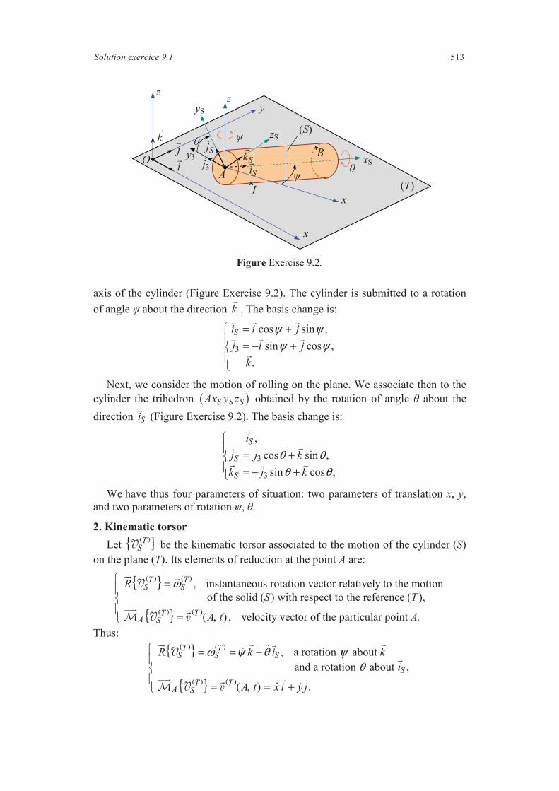
Solution exercice 9.1 513
Figure Exercise 9.2.
axis of the cylinder (Figure Exercise 9.2). The cylinder is submitted to a rotation
of angle about the direction k
. The basis change is:
3
cos sin ,
sin cos ,
.
Si i j
j i j
k
ψ ψ
ψ ψ
= +
= − +
Next, we consider the motion of rolling on the plane. We associate then to the
cylinder the trihedron ( )S S SAx y z obtained by the rotation of angle about the
direction Si
(Figure Exercise 9.2). The basis change is:
3
3
,
cos sin ,
sin cos ,
S
S
S
i
j j k
k j k
θ θ
θ θ
= + = − +
We have thus four parameters of situation: two parameters of translation x, y,
and two parameters of rotation , .
2. Kinematic torsor
Let ( ) TS be the kinematic torsor associated to the motion of the cylinder (S)
on the plane (T). Its elements of reduction at the point A are:
( ) ( )
( ) ( )
, instantaneous rotation vector relatively to the motion
of the solid ( ) with respect to the reference ( ),
( , ) , velocity vector of the particular point .
T TS S
T TA S
R
S T
A t A
ω =
=
Thus: ( ) ( )
( ) ( )
, a rotation about
and a rotation about ,
( , ) .
T TS S S
S
T TA S
R k i k
i
A t x i y j
ω ψ θ ψθ
= = +
= = +
(T)
(S)
A
B
x
x
xS
yS y z
O
z
ijk
Si
Sj
3j
Sk
y3
zS
I

Solution Exercise 9.3 514
The instantaneous rotation vector depends only on the parameters of rotation and
the velocity vector depends only on the parameters of translation.
3. Kinematic vectors of a point of the solid As an example, we consider the case of the point B of the cylinder (Figure
Exercise 9.2) contained in the plane ( )S SAx y . Its coordinates relatively to the
system ( )S S SAx y z are: l, a, 0 where l is the length of the cylinder. Thus:
S SAB l i a j= +
.
3.1. Velocity vector
The expression of the moment at the point B of the kinematic torsor leads to: ( ) ( ) ( )
( , ) ( , )T T TSB t A t ABω= + ×
.
The calculation of the vector product ( )TS ABω ×
is easier in the basis ( ), , S Si j k
.
However, the vector ( )
( , )T A t is expressed in the basis ( ), , i j k
. There exist
then several possibilities to implement the calculation. For example, we may carry
out all the calculations in the basis ( ), , i j k
. In this way, we transform the com-
ponents of the vectors in this basis:
( ) cos sinT
S Sk i i j kω ψ θ θ ψ θ ψ ψ= + = + + ,
( ) ( ) cos sin cos sin cos cos sinS SAB l i a j l a i l a j a kψ ψ θ ψ ψ θ θ= + = − + + +
.
After derivation of the vector product ( )TS ABω ×
, we obtain:
( ) ( )
( )
( , ) sin cos cos sin sin
cos sin cos cos sin cos .
T B t x l a a i
y l a a j a k
ψ ψ ψ θ θ ψ θ
ψ ψ ψ θ θ ψ θ θ θ
= − + +
+ + − − +
3.2. Acceleration vector
The acceleration vector can be obtained either by derivation of the preceding
expression, or using Relation (9.24).
9.3 Motion of two solidsThe process of analysis is again the same.
1. Parameters of situation
1.1. Motion of the solid (S1) with respect to the support (T)
We associate a coordinate system (Oxyz) to the support (T), such as the axis Oy
coincides with the axis (1) and the axis Ox
is downward vertical (Figure Exercise
9.3). The axis Oz
has then the same direction as the axis of rotation (2).
1.1.1. Parameters of translation
We choose a particular point of the solid (S1): the point A1. The coordinates of
the point are (0, y, 0). The solid (S1) has one parameter of translation y.
1.1.2. Parameters of rotation
We associate a trihedron attached to the solid (S1): (A1xyz). This system keeps
the same directions during the motion. There is thus no parameter of rotation.

Solution exercice 9.1 515
Figure Exercise 9.3.
1.2. Motion of the solid (S2) with respect to the solid (S1)
A coordinate system is already associated to the solid (S1).
1.2.1. Parameters of translation
We have to choose a particular point of the solid (S2): the point A1. It is fixed
relatively to the solid (S1). There is thus no parameter of translation.
1.2.2. Parameters of rotation
We associate a coordinate system attached to the solid (S2): the system (A1x2y2z)
such as the axis 21A x
passes through the point A2. The system is obtained from
the system (A1xyz) through a rotation of angle about the direction .k
We have
thus one parameter of rotation . The basis change is:
2
2
cos sin ,
sin cos ,
.
i i j
j i j
k
ψ ψ
ψ ψ
= +
= − +
2. Kinematic torsors
2.1. Motion of the solid (S1) with respect to the support (T)
Let ( ) 1
TS be the kinematic torsor relative to the motion of the solid (S1) with
respect to the support (T). Its elements of reduction at the point A1 are:
( ) ( )
( ) ( )
1 1
1 11 1
0, instantaneous rotation vector,
( , ) , velocity vector of point with respect to ( ).
T TS S
T TA S
R
A t y j A T
ω = =
= =
2.2. Motion of the solid (S2) with respect to the solid (S1)
Let ( ) 1
2
S
S be the kinematic torsor relative to the motion of the solid (S2) with
respect to the solid (S1). Its elements of reduction at the point A1 are:
(T) (R) (S1)
(S2)
A2
A1 (1)
(2) y
x
x x2
y2
z
z
d
O

Solution Exercise 9.3 516
( ) ( )
( ) ( )
1 1
2 2
1 11 2
1 1 1
, instantaneous rotation vector,
( , ) 0, velocity vector of point with respect to ( ).
S S
S S
S SA S
R k
A t A S
ω ψ = = = =
2.3. Motion of the solid (S2) with respect to the support (T)
Let ( ) 2
TS be the kinematic torsor relative to the motion of the solid (S2) with
respect to the support (T). Its elements of reduction can be obtained either directly,
or using the relation of combination of motions:
( ) ( ) ( ) 1
2 2 1
ST TS S S
= + .
Thus, we deduce the elements of reduction at the point A1:
( ) ( ) ( ) ( ) ( ) ( ) ( ) ( )
1
2 2 2 1
11 1 12 2 1
1
,
( , ) .
ST T TS S S S
ST T TA A AS S S
R R R k
A t y j
ω ψ = = + = = = + =
3. Kinematic vectors of the point A2
We have:
21 2A A a i=
.
3.1. Velocity vector
From the expression of the moment at the point A2 of the kinematic torsor, we
obtain:
( ) ( ) ( )
222 1 1( , ) ( , )T T T
SA t A t A Aω= + ×
.
Hence: ( )
2 2( , )T A t y j a jψ= +
,
or considering the basis change:
( ) ( )2( , ) sin cosT A t a i y a jψ ψ ψ ψ= − + +
.
3.2. Acceleration vector
The vector is obtained by deriving the preceding expression. Thus:
( ) ( ) ( )2 22( , ) sin cos cos sinTa A t a i y a jψ ψ ψ ψ ψ ψ ψ ψ = − + + + −
.

Chapter 10
Kinematics of Rigid Bodies in Contact
10.1 Motion of a wheel on a straight line (Figure 10.14)
This motion can also be applied to the motion of a cylinder on a plane, when
there is no spinning of the cylinder.
The kinematic analysis of solids in contact is first implemented by the same
process as the one used in the exercises of the preceding chapter. The conditions
of sliding, spinning and rolling are next considered.
1. Parameters of situation We choose a coordinate system attached to the reference (T) containing the line
(D). Thus the system (Oxyz) such as the axis Ox
coincides with the line (D) and
the plane (Oxy) contains the plane of the wheel (Figure Exercise 10.1).
1.1. Parameters of translation
We choose a particular point of the wheel (S), defined with the smallest
number of parameters depending on time: the centre A of the wheel. The coordi-
nates of the point A relatively to (Oxyz) are (x, a, 0). The position vector is:
OA x i a j= +
,
where a is the radius of the wheel.
We have thus one parameter of translation: x.
1.2. Parameters of rotation
We associate a trihedron attached to the wheel: the system ( )S SAx y z (Figure
Exercise 10.1). The orientation of the wheel is then given by the rotation of angle
ψ and direction k
. The basis change is written:
Figure Exercise 10.1.
I
A(S)
(D) MO
y
x
z
z
y
x
xS
yS
(T)
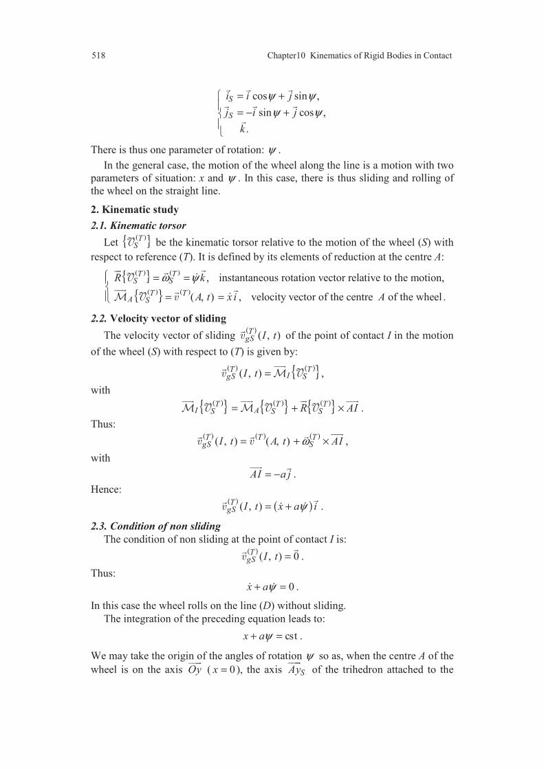
518 Chapter10 Kinematics of Rigid Bodies in Contact
cos sin ,
sin cos ,
.
S
S
i i j
j i j
k
ψ ψ
ψ ψ
= +
= − +
There is thus one parameter of rotation: ψ .
In the general case, the motion of the wheel along the line is a motion with two
parameters of situation: x and ψ . In this case, there is thus sliding and rolling of
the wheel on the straight line.
2. Kinematic study
2.1. Kinematic torsor
Let ( ) TS be the kinematic torsor relative to the motion of the wheel (S) with
respect to reference (T). It is defined by its elements of reduction at the centre A:
( ) ( )
( ) ( )
, instantaneous rotation vector relative to the motion,
( , ) , velocity vector of the centre of the wheel .
T TS S
T TA S
R k
A t x i A
ω ψ = =
= =
2.2. Velocity vector of sliding
The velocity vector of sliding ( )
( , )TgS I t of the point of contact I in the motion
of the wheel (S) with respect to (T) is given by:
( ) ( ) ( , )T TIgS SI t =
,
with ( ) ( ) ( ) T T T
I AS S SR AI= + × .
Thus: ( ) ( ) ( )
( , ) ( , )T T TgS SI t A t AIω= + ×
,
with
AI a j= −
.
Hence: ( ) ( )( , )TgS I t x a iψ= +
.
2.3. Condition of non sliding
The condition of non sliding at the point of contact I is: ( )
( , ) 0TgS I t =
.
Thus:
0x aψ+ = .
In this case the wheel rolls on the line (D) without sliding.
The integration of the preceding equation leads to:
cstx aψ+ = .
We may take the origin of the angles of rotation ψ so as, when the centre A of the
wheel is on the axis Oy
( 0x = ), the axis SAy
of the trihedron attached to the

Solution Exercise 10.1 519
wheel coincides with the axis Oy
. In this case, we have 0ψ = for 0x = and the
preceding equation is written:
0x aψ+ = .
The parameters x and have opposed signs. When the wheel moves in the direc-
tion of 0x < , is positive: the wheel rolls in the direct sense. When the wheel
moves in the direction 0x > , is negative: the wheel rolls in the inverse sense.
The motion has only one parameter of situation: x or .
3. Motion of a point of the wheel
3.1. Kinematic vectors
We consider the point M located on the circumference of the wheel and on the
axis SAy
(Figure Exercise 10.1) of Cartesian coordinates ( )0, , 0a− relatively
to the system ( )S SAx y z . Thus: SAM a j= −
.
The velocity vector of the point M is given by:
( ) ( ) ( ) ( , ) ( , )T T T
SM t A t AMω= + ×
,
thus: ( )
( , )TS SM t x i k a j x i a iψ ψ= + × − = +
.
Hence: ( ) ( )( , ) cos sinT M t x a i a jψ ψ ψ ψ= + +
.
The acceleration vector is then deduced using the relation:
( )( )
( )
d( , ) ( , )d
TT Ta M t M t
t=
.
We obtain: ( ) ( ) ( )2 2( , ) cos sin sin cosTa M t x a i a jψ ψ ψ ψ ψ ψ ψ ψ = + − + +
.
When the wheel rolls without sliding, the kinematic vectors are written: ( ) ( )[ ]( , ) 1 cos sinT M t a i jψ ψ ψ= − + +
,
( ) ( ) ( ) 2 2( , ) 1 cos sin sin cosTa M t a i jψ ψ ψ ψ ψ ψ ψ ψ = − + − + +
.
These expressions can also be expressed as a function of the parameter x.
3.2. Trajectory
The trajectory of the point M relatively to the system (Oxyz) is deduced from
the expression of its position vector:
OM OA AM= +
.
Thus:
( ) sin cosSOM x i a j x a i a jψ ψ= − = + −
.
This trajectory depends on the variations of the parameters x and ψ as functions
of time.
In the case where the wheel rolls without sliding, the position vector is written:
( ) ( )sin 1 cosOM a i a jψ ψ ψ= − + + −
.

520 Chapter10 Kinematics of Rigid Bodies in Contact
This expression is identical to Expression (7.76) with qψ = − .
10.2 Motion of a cylinder (or a sphere) inside a cylinder (Figure 10.15)
We study the motion of a cylinder or a sphere, in such a way that the centre of
the cylinder or the sphere moves in the same vertical plane during the motion.
1. Parameters of situation We associate a trihedron attached to the cylinder (T): (Oxyz), so as the axis
Oz
coincides with the axis of the cylinder and the axis Ox
is upwards vertical
(Figure Exercise 10.2).
1.1. Parameters of translation
We choose a particular point of the cylinder or of the sphere (S), so as this
point is defined with the smallest number of parameters depending of time. Thus
the point OS centre of the cylinder or of the sphere. The position of the point OS is
defined by the angle α between the axes SOO
and Ox
. We have thus one para-
meter of translation: α , which is in fact one of the cylindrical coordinates of the
point OS.
The position vector of the point OS is given by:
( )1SOO b a i= −
,
where b and a are the respective radii of the cylinders (T) and (S), and where 1i
is
the unit direction vector of SOO
:
1 cos sini i jα α= +
.
1.2. Parameters of rotation
We associate a coordinate system attached to the cylinder or to the sphere: the
system ( )S S SO x y z (Figure Exercise 10.2). The orientation is then given by the
angle of rotation ψ about the direction k
. The basis change is written:
Figure Exercise 10.2.
(S)
I
(T)
M
O
y
z
y
xxS
yS
OS
z
x
i
j
1i
Si
Sj

Solution Exercise 10.2 521
cos sin ,
sin cos ,
.
S
S
i i j
j i j
k
ψ ψ
ψ ψ
= +
= − +
Finally the motion has two parameters of situation: , .α ψ
2. Kinematic study
2.1. Kinematic torsor
Let ( ) TS be the kinematic torsor associated to the motion of the cylinder or
of the sphere (S) with respect to the cylinder (T). Its elements of reduction at the
point SO are:
( ) ( )
( ) ( )
, instantaneous rotation vector relative to the motion,
( , ) , velocity vector of the point
with respect to the cylinder ( ) .S
T TS S
T TO S S S
R k
O t O
T
ω ψ = =
=
With:
( )( )
( )1
d( , )
d
TT
SSO t OO b a jt
α= = −
.
2.2. Velocity vector of sliding
The velocity vector of sliding ( )
( , )TgS I t of the point of contact I in the motion
of the cylinder or of the sphere (S) with respect to the cylinder (T) is given by:
( ) ( ) ( , )T TIgS SI t =
.
The expression of the moment leads to:
( ) ( ) ( )( , ) ( , )T T T
gS S S SI t O t O Iω= + ×
,
with
1SO I a i=
.
Hence: ( ) ( )[ ] 1( , )TgS I t b a a jα ψ= − +
.
The velocity vector of sliding is collinear to the direction 1j
of the plane tangent
to the two solids at the point of contact I.
2.3. Condition of non sliding
The condition of non sliding at the point of contact I is written: ( )
( , ) 0TgS I t =
.
Thus: ( ) 0b a aα ψ− + = .
In this case, the cylinder or the sphere rolls on the cylinder (T) without sliding.
The motion is then a motion with only one parameter of situation or .α ψ
The integration of the preceding equation leads to:

522 Chapter10 Kinematics of Rigid Bodies in Contact
( ) cstb a aα ψ− + = .
Taking the origin of the angle ψ so as, when the centre SO is on the axis Ox
, the
axis S SO x
of the trihedron attached to the solid (S) coincides with the axis Ox
,
we have 0ψ = for 0α = . The preceding equation is then written as:
( ) 0b a aα ψ− + = .
The angle of rotation is thus expressed as:
b a
aψ α−
= − .
The signs of the angles and ψ α are opposed. When the cylinder or the sphere
(S) moves in the direction of 0α > , (S) rolls in the inverse sense. And conversely.
3. Motion of a point We consider the point M located on the axis S SO x
on the periphery of the
solid (S) (Figure Exercise 10.2) of Cartesian coordinates ( ), 0, 0a relatively to
the system ( )S S SO x y z . Thus: S SO M a i=
.
3.1. Kinematic vectors
The velocity vector of the point M at the instant t is expressed by:
( ) ( ) ( ) ( , ) ( , )T T T
S S SM t O t O Mω= + ×
,
Hence: ( ) ( ) ( )
1 1( , )TS SM t b a i k a i b a i a jα ψ α ψ= − + × = − +
.
Thus: ( ) ( )[ ]
( )[ ]
( , ) cos sin
sin cos .
T M t b a a i
b a a j
α α ψ ψ
α α ψ ψ
= − −
+ − +
The acceleration vector is obtained by deriving the velocity vector. Hence:
( ) ( ) ( ) ( )( )( ) ( )
2 2
2 2
( , ) cos sin sin cos
sin cos cos sin .
Ta M t b a a i
b a a j
α α α α ψ ψ ψ ψ
α α α α ψ ψ ψ ψ
= − − − +
+ − + + −
3.2. Trajectory
The trajectory of the point M relatively to the system (Oxyz) is deduced from
the expression of its position vector:
S SOM OO O M= +
.
Thus:
( )1 SOM b a i a i= − +
,
or
( )[ ] ( )[ ]cos cos sin sinOM b a a i b a a jα ψ α ψ= − + + − +
.
This trajectory depends of the variations of the parameters α and ψ as functions
of time, according to the conditions of sliding and rolling.
In the case where there is rolling without sliding, the position vector is given by:

Solution Exercise 10.2 523
( ) ( )cos cos sin sinb a b aOM b a a i b a a ja a
α α α α− − = − + + − −
.
The trajectory is a hypocycloïde.
10.3 Cylinder on a planeThe case of a cylinder in contact with a plane was studied in Exercice 9.2. We
consider (Figure Exercise 9.2) a point I of contact between the cylinder and the
plane distant of 1x from the side of the cylinder. The coordinates of this point
relatively to the system ( )S SAx y z are: ( )1, 0, x a− . The position vector is thus
written:
1 SAI x i a k= −
.
The velocity vector of sliding of the point of contact I in the motion of the
cylinder (S) with respect to the plane (T) is: ( ) ( ) ( )
( , ) ( , )T T TgS SI t A t AIω= + ×
.
The vector product is:
( ) ( )3
1 3
1
0
0
ST
S
i j k
AI x a j
x a
ω θ ψ ψ θ× = = +
.
We obtain thus: ( ) ( ) ( )1 1( , ) sin cosTgS I t x x a i y x a jψ θ ψ ψ θ ψ = − + + + +
.
There is non sliding at the points I such as ( )
( , ) 0.TgS I t =
Thus at the points I
such as:
( )
( )1
1
sin 0,
cos 0.
x x a
y x a
ψ θ ψ
ψ θ ψ
− + =
+ + =
Case where the cylinder does not spin We consider the case where there is non spinning of the cylinder. Thus 0ψ = .
The velocity vector of sliding of the point I of contact is thus written as:
( ) ( ) ( )( , ) sin cosTgS I t x a i y a jθ ψ θ ψ= − + +
.
The velocity vector of sliding is then independent of the abscissa x1, thus the same
for all the points of the generator of contact.
The case of rolling without sliding nor spinning leads thus to:
sin 0,
cos 0.
x a
y a
θ ψ
θ ψ
− =
+ =
By excluding θ , we obtain: tan 0x y ψ+ = . Then integrating:
tan cstx y ψ+ = .
The constant depends on the position of the cylinder at the initial instant. The
trajectory of the point A is thus the straight line of orientation .ψ

Chapter 11
General Elements on the Mechanical Actions
11.1 Mechanical action exerted on a frame (Figure 11.5)
11.1.1. Field of the forces exerted
We have first to characterize the field of the forces i. At each point Mi it is
exerted a force of resultant iR
, of which the characteristics are deduced from the
data and Figure 11.5. Note that to express the components of a force of magnitude
Ri and direction iα (Figure Exercise 11.1), it is advised to use the relations:
( ) cos , sin , 0i i i i iR R Rα α
.
Thus, the field of forces is:
M1 (4, 0, 0) 1R
(0, –2000, 0)
M2 (8, 0, 0) 2R
(0, –1000, 0)
M3 (12, 0, 0) 3R
(0, –1500, 0)
M4 (2, 1,5, 0) 4R
(–900, 1200, 0)
M5 (6, 4, 0) 5R
(–447, 894, 0)
M6 (14, 4, 0) 6R
(–671, –1342, 0)
M7 (18, 1,5, 0) 7R
(–1200, –1600, 0)
11.1.2. Action exerted on the frame
Let ( ) S be the torsor representing the resultant of the mechanical action
exerted on the frame (S).
1.Resultant of the action
The resultant is:
( ) 7
1
i
i
R S R
=
=
.
Thus: ( ) 3218 5348R S i j= − − .
Figure Exercise 11.1.
x
y
iα
iR
iR

524 Chapter 11 General Elements on the Mechanical Actions
2. Moment of the action at the point O
The moment at the point O is expressed by:
( ) 7
1
iiO
i
S OM R
=
= ×
.
We have:
1 21 2
3 43 4
5 65 6
77
8000 , 8000 ,
18000 , 3750 ,
7152 , 16104 ,
27000 .
OM R k OM R k
OM R k OM R k
OM R k OM R k
OM R k
× = − × = −
× = − × =
× = × = −
× = −
Hence:
( ) 66202O S k= − .
3. Type of action
The scalar invariant of the torsor is:
( ) ( ) ( ) 0OI S R S S= =⋅
.
The mechanical action exerted is thus a force.
4. Support of the force
It is the set of the points P such as ( ) 0P S = . We evaluate the moment
at the point P of coordinates (x, y, z):
( ) ( ) ( ) P OS S R S OP= + ∧
.
Thus:
( ) ( ) 5348 3218 5348 3218 66202P S z i z j x y k= − + + − − .
The equation of the support of the force is then:
0,
5348 3218 66202 0.
z
x y
=
− − =
The support is contained in the plane (Oxy). We may determine two points of the
support:
A (0, 20.57, 0) and B (12.38, 0, 0).
11.2 Mechanical action exerted on a barrage11.2.1. The action exerted by the water on an elementary surface dS(M) of the
barrage surrounding the point M is a force of resultant:
d ( ) ( ) d ( )R M p M S M i=
,
and support ( ), M i
.
The pressure p(M) exerted at the point M results from the atmospheric pressure
0p and the height h z− of the water which is above the point M. Thus:

Solution Exercise 11.2 525
( )0( )p M p g h zρ= + − .
This expression can be written in the form:
( )p M zλ µ= + ,
introducing the coefficients:
0 , .p gh gλ ρ µ ρ= + = −
11.2.2. The action exerted by the water of the dam on the side (D) of the barrage
in contact with the water is represented by the torsor ( ) .D
1. Resultant
The resultant is:
( ) ( ) ( )
d ( ) ( )d ( )D D
R D R M i p M S M= = .
Thus, introducing the Cartesian coordinates (0, y, z) of the point M, it comes:
( ) ( )
0 0
d da h
y z
R D i z y zλ µ= =
= + .
The integration leads to:
( ) ( ) ( )
2 2h hR D ah i S iλ µ λ µ= + = +
,
where S is the area of the face of the barrage.
Numerical application
3 3 2 5010 kg m , 9.81 m s , 1.013 10 Pa, 50 m, 30 m.g p a hρ − − −= = = × = =
Hence: 5 3 13.956 10 Pa, 9.81 10 Pa m .λ µ −= × = − ×
Thus: 87.45 10 (en N).R i= ×
2. Moment
It is needed to determine the moment at a point or to find a point which is asso-
ciated to a particular property for the moment.
Here the field of forces is such as:
( )M D∀ ∈ d ( ) ( ) d ( )R M p M S M i=
.
At any point M of the face of the barrage it is associated a force (a slider) of
support (of axis) i
which is independent of the point M. We are in the case
studied in Section 5.3.3. From the results established in this section, there exists a
measure centre H, here a centre of thrust. This centre is such as the moment at the
point H of the torsor ( ) D is null. Thus, the determination of the measure
centre stands in for the determination of the moment at a point.
The position of the centre of thrust H is given, from Expression (5.72), by:
( ) ( )
1 ( ) d ( )D
OH OM p M S MDµ
=
,
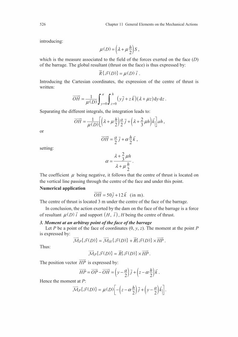
526 Chapter 11 General Elements on the Mechanical Actions
introducing:
( ) ( )2hD Sµ λ µ= + ,
which is the measure associated to the field of the forces exerted on the face (D)
of the barrage. The global resultant (thrust on the face) is thus expressed by:
( ) ( )R D D iµ= .
Introducing the Cartesian coordinates, the expression of the centre of thrust is
written:
( )( )( )
0 0
1 d da h
y z
OH y j z k z y zD
λ µµ = =
= + +
.
Separating the different integrals, the integration leads to:
( ) ( ) ( )1 22 2 3h aOH j h k ah
Dλ µ λ µ
µ = + + +
,
or
2 2a hOH j kα= +
,
setting:
23
2
h
h
λ µα
λ µ
+=
+.
The coefficient µ being negative, it follows that the centre of thrust is located on
the vertical line passing through the centre of the face and under this point.
Numerical application
50 12 (in m).OH j k= +
The centre of thrust is located 3 m under the centre of the face of the barrage.
In conclusion, the action exerted by the dam on the face of the barrage is a force
of resultant ( )D iµ
and support ( ), H i
, H being the centre of thrust.
3. Moment at an arbitray point of the face of the barrage
Let P be a point of the face of coordinates (0, y, z). The moment at the point P
is expressed by:
( ) ( ) ( ) P HD D R D HP= + ×
.
Thus:
( ) ( ) P D R D HP= ×
.
The position vector HP
is expressed by:
( ) ( )2 2a hHP OP OH y j z kα= − = − + −
.
Hence the moment at P:
( ) ( ) ( ) ( )2 2P
h aD D z j y kµ α = − − + −
.
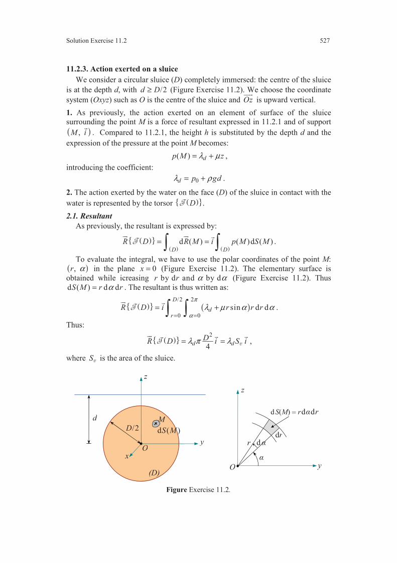
Solution Exercise 11.2 527
11.2.3. Action exerted on a sluice We consider a circular sluice (D) completely immersed: the centre of the sluice
is at the depth d, with /2d D≥ (Figure Exercise 11.2). We choose the coordinate
system (Oxyz) such as O is the centre of the sluice and Oz
is upward vertical.
1. As previously, the action exerted on an element of surface of the sluice
surrounding the point M is a force of resultant expressed in 11.2.1 and of support
( ), M i
. Compared to 11.2.1, the height h is substituted by the depth d and the
expression of the pressure at the point M becomes:
( ) dp M zλ µ= + ,
introducing the coefficient:
0d p gdλ ρ= + .
2. The action exerted by the water on the face (D) of the sluice in contact with the
water is represented by the torsor ( ) .D
2.1. Resultant
As previously, the resultant is expressed by:
( ) ( ) ( )
d ( ) ( )d ( )D D
R D R M i p M S M= = .
To evaluate the integral, we have to use the polar coordinates of the point M:
( ), r α in the plane 0x = (Figure Exercise 11.2). The elementary surface is
obtained while icreasing by d and by dr r α α (Figure Exercise 11.2). Thus
d ( ) d dS M r rα= . The resultant is thus written as:
( ) ( )
/2 2
0 0
sin d dD
dr
R D i r r rπ
αλ µ α α
= == +
.
Thus:
( ) 2
4d d
DR D i S iλ π λ= =
,
where S
is the area of the sluice.
Figure Exercise 11.2.
z
x
y
M
d ( )S M/2D
O
d
(D)y
z
O
d
d S(M) = rddr
rdr
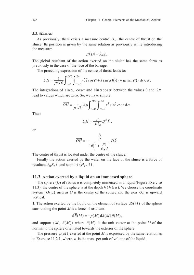
528 Chapter 11 General Elements on the Mechanical Actions
2.2. Moment
As previously, there exists a measure centre H
, the centre of thrust on the
sluice. Its position is given by the same relation as previously while introducing
the measure:
( )dD Sµ λ=
.
The global resultant of the action exerted on the sluice has the same form as
previously in the case of the face of the barrage.
The preceding expression of the centre of thrust leads to:
( )( )( )
/2 2
0 0
1 cos sin sin d dD
dr
OH r j k r r rD
π
αα α λ µ α α
µ = == + +
.
The integrations of sin , cos and sin cosα α α α between the values 0 and 2πlead to values which are zero. So, we have simply:
( )
/2 23 2
0 0
1 sin d dD
r
OH k r rD
π
αµ α α
µ = ==
.
Thus:
2
16 d
OH D kµλ
=
,
or
016 1
DdOH D k
p
gdρ
= − +
.
The centre of thrust is located under the centre of the sluice.
Finally the action exerted by the water on the face of the sluice is a force of
resultant d S iλ
and support ( ), H i
.
11.3 Action exerted by a liquid on an immersed sphereThe sphere (D) of radius a is completely immersed in a liquid (Figure Exercise
11.3): the centre of the sphere is at the depth h ( h a≥ ). We choose the coordinate
system (Oxyz) such as O is the centre of the sphere and the axis Oz
is upward
vertical.
1. The action exerted by the liquid on the element of surface d ( )S M of the sphere
surrounding the point M is a force of resultant:
d ( ) ( ) d ( ) ( )R M p M S M n M= −
,
and support ( ), ( )M n M−
where ( )n M
is the unit vector at the point M of the
normal to the sphere orientated towards the exterior of the sphere.
The pressure ( )p M exerted at the point M is expressed by the same relation as
in Exercise 11.2.1, where ρ is the mass per unit of volume of the liquid.

Solution Exercise 11.3 529
Figure Exercise 11.3.
2. Action exerted by the liquid on the sphere
The action exerted on the sphere (D) is represented by the torsor ( ) .D
2.1. Resultant
The resultant is expressed by:
( ) ( ) ( )
d ( ) ( ) ( )d ( )D D
R D R M p M n M S M= = − .
The evaluation of the integral is implemented while using the spherical coor-
dinates of the point M (Figure Exercise 11.3). The point M is located on the
sphere by its longitude α and its latitude β . The elementary surface is obtained
by increasing the longitude and the latitude by dα and dβ , respectively. Thus:
2d ( ) cos d dS M a β α β= .
The unit vector ( )n M
at the point M is expressed by:
( ) ( , ) ( ) cos sinn M n u kα β α β β= = +
,
where ( )u α
is the unit vector of the longitude α . Hence:
( ) cos cos sin cos sinn M i j kα β α β β= + +
.
The resultant is thus expressed by:
( )
( ) ( )
22 2
02
sin cos cos sin cos sin cos d d .
R D
a i j k a
ππ
πα βλ µ β α β α β β β α β
= =−
=
− + + +
The integrations of sin and cosα α between 0 and 2π give null values. Hence:
( ) ( )
222
02
sin sin cos d dR D k a a
ππ
πα βλ µ β β β α β
= =−= − +
,
z
x
y
M
d ( )S M
O
h
(D)
( )n M
x
yO
d
d S(M) = a
2cos dd
z
a
d
a cos a cos d
i
j
k
( )u α

Solution Exercise 11.3 530
or
( )
223 2
02
sin cos d dR D a k
ππ
πα βµ β β α β
= =−= −
.
Thus:
( ) 343
R D a g kπ ρ= ,
or
( ) R D mg k= ,
where m is the mass of liquid having the same volume as the sphere.
2.2. Moment
In the present case, the normal ( )n M
at every element of surface of the sphere
depends on the point M. Thus, there does not exist a measure centre.
We determine the moment at the centre O of the sphere expressed by:
( ) ( )
d ( )OD
D OM R M= ×
,
or
( ) ( )
( ) ( )d ( )OD
D OM n M p M S M= − × .
The vectors OM
and ( )n M
are collinear. So, it follows that their vector pro-
duct is null. Hence:
( ) 0O D = .
In conclusion, the mechanical action exerted by the liquid on the sphere is a
force of which the resultant has a magnitude mg and the support is the downward
vertical axis passing through the centre of the sphere.
Hence the result: the mechanical action exerted by the liquid on the sphere is
opposed to the action of gravity (Chapter 12) exerted on the mass of liquid
occupying the same volume as the sphere. This result is described by the Principle
of Archimedes which is applied to a solid with an arbitrary shape immersed in a
liquid.

Chapter 12
Gravitation. Gravity
Mass Centre
12.1 Mass centre of an arc of circle (figure 12.13)
We take (Figure Exercise 12.1) the coordinate system (Oxyz) such as the point
O is the centre of the circle on which the arc is constructed, the plane (Oxy) con-
tains the arc of circle and the axis Ox
coincides with the axis of symmetry.
The solid being homogeneous, the mass centre coincides with the centroid
given by Expression (12.47). A point M of the arc of circle can be located by its
polar angle θ (Figure Exercise 12.1). The length of an element of arc, obtained
while increasing θ by dθ , is da θ . The total length of the arc is 2aα . Expres-
sion (12.47) is thus written:
( )1 cos sin d2
OG a i j aa
α
αα α θ
α −= +
.
Hence:
sinOG a iαα
=
.
12.2 Mass centre of a circular sector (Figure 12.14)
The mass centre coincides with the centroid. A point M of the sector (Figure
Exercise 12.2) is characterized by its polar coordinates ( ), r θ and the element of
surface of the sector is obtained while increasing r by dr and θ by dθ . Its area is
d d .r rθ The surface of the sector is 2.aα Expression (12.47) is thus written:
( )
20
1 cos sin d da
r
OG r i j r ra
α
θ αα α θ
α = =−= +
.
Hence: 2 sin3
OG a iαα
=
.
Figure Exercise 12.1. Figure Exercise 12.2.
a
M
O
y
x
z
a
M
O
y
x
z
r
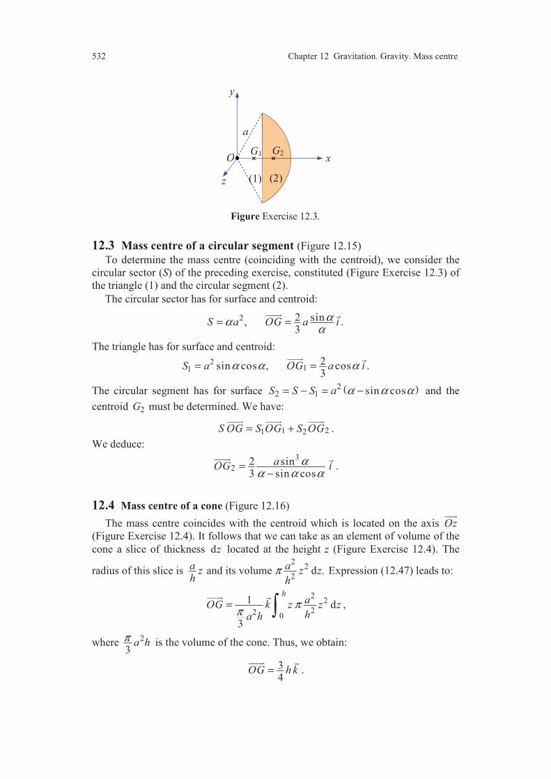
532 Chapter 12 Gravitation. Gravity. Mass centre
Figure Exercise 12.3.
12.3 Mass centre of a circular segment (Figure 12.15)
To determine the mass centre (coinciding with the centroid), we consider the
circular sector (S) of the preceding exercise, constituted (Figure Exercise 12.3) of
the triangle (1) and the circular segment (2).
The circular sector has for surface and centroid:
2 2 sin, .3
S a OG a iααα
= =
The triangle has for surface and centroid:
211
2sin cos , cos .3
S a OG a iα α α= =
The circular segment has for surface ( )22 1 sin cosS S S a α α α= − = − and the
centroid 2G must be determined. We have:
1 21 2S OG S OG S OG= +
.
We deduce: 3
22 sin3 sin cos
aOG iαα α α
=−
.
12.4 Mass centre of a cone (Figure 12.16)
The mass centre coincides with the centroid which is located on the axis Oz
(Figure Exercise 12.4). It follows that we can take as an element of volume of the
cone a slice of thickness dz located at the height z (Figure Exercise 12.4). The
radius of this slice is a zh
and its volume2
2
2d .a z z
hπ Expression (12.47) leads to:
22
22 0
1 d
3
haOG k z z zha h
ππ
=
,
where 2
3a hπ is the volume of the cone. Thus, we obtain:
34
OG h k=
.
a
G1O
y
x
z
G2
(1) (2)

Solution Exercise 12.5 533
Figure Exercise 2.4.
12.5 Mass centre of a spherical segment (Figure 12.17)
We choose (Figure Exercise 12.5) a coordinate system (Oxyz) such as O is the
centre of the base of the segment and Oz
is the axis of symmetry. The mass
centre coincides with the centroid of the segment which is located on the axis Oz
.
As in the preceding exercise, we can take for an element of volume a slice of
thickness dz located at the height z. The radius r of this slice is such as:
( ) ( ) ( )22 2 2 2 2r a z a h z a h z a h h= − + − = − − − + − .
Expression (12.47) leads to:
( ) ( )[ ]
2
0
2 2 dh
OG k z z a h z a h h zVπ= − − − + −
,
where V is the volume of the spherical segment expressed by:
( )2 33
V h a hπ= − .
The integration leads to:
( )414 3
a h hOG ka h−=−
.
Figure Exercise 12.5.
h
a
z
dz
z
y
x
O
h
aOz
dz
z
y
x
r

534 Chapter 12 Gravitation. Gravity. Mass centre
Figure Exercise 12.6.
12.6 Mass centre of a hollowed cylinder (Figure 12.18)
The solid cylinder (S) can be considered as the union of the hollowed cylinder
(S1) and of the cylinder (S2) which is hollowed out.
The solid cylinder (S) has a volume 2V a hπ= and its mass centre G has for
coordinatees (0, 0, 2h ).
The cylinder (S2) which is hollowed out has a volume 2
24
aV hπ= and its mass
centre G2 has for coordinates (0, , )2 2a h .
Te hollowed cylinder (S1) has a volume 21 2
34
V V V a hπ= − = and a mass
centre G1 which is to be determined.
From Relation (12.41), we have:
22 2
1 23 4 4
aa h OG a h OG h OGπ π π= +
.
Thus:
16 2a hOG j k= − +
.
The coordinates of G are (0, , )6 2a h− .
12.7 Action of gravitation exerted by a sphereThe action of gravitation exerted by a sphere at a point M external to the sphere
is defined in Section 12.1.3. Its moment at the point M is null and its resultant
h
a
z
y
x
/2a
O

Solution Exercise 12.7 535
Figure Exercise 12.7.
is expressed by Relation (12.7). To determine this resultant, it is necessary to use
the spherical coordinates of the point M ′ of the sphere. For that, we choose the
coordinate system (Oxyz) such as the axis Oz
passes through the point M (Figure
Exercise 12.7). The spherical coordinates and the element of volume of the sphere
are considered in Subsection 15.4.3.2 of Chapter 15. Using the results of this
subsection, Expression (12.7) of the resultant is written:
( )
22 2
30 0
2
( ) cos d d da
R
MMR Km M R RS MMM
ππ
πα βρ β α β
= = =−
′ ′=→′
.
The vector MM ′
is expressed as:
( )MM OM OM R n M r k′ ′ ′= − = −
,
where r is the distance from the point M to the centre O of the sphere and ( )n M ′
is the unit vector of ,OM ′
already introduced in Exercise 11.3. This vector is
expressed as:
( ) ( , ) ( ) cos sinn M n u kα β α β β′ = = +
,
where the vector ( )u α
is the unit vector of the direction α :
( ) cos sinu i jα α α= +
.
We have thus:
( ) ( )cos sinMM R u R r kβ α β′ = + −
.
Hence:
( ) ( )
1 122 2 2 22 2cos sin 2 sinMM MM R R r R r rRβ β β ′ ′= = + − = + −
.
Moreover, the mass per unit volume is a function of , , and R α β :
( ) ( , , )M Rρ ρ α β′ = .
z
x
y
M ′d ( )V M ′
O
( )n M ′
M
a
r

536 Chapter 12 Gravitation. Gravity. Mass centre
The resultant is thus written:
( ) ( )
( )
22 2
30 0 2 2 22
cos sin( , , ) cos d d d .
2 sin
a
R
R S M
R u R r kKm R R R
R r rR
ππ
πα β
β α βρ α β β α β
β= = =−
=→
+ −
+ −
To continue the integration, it is necessary to introduce assumptions on the
mass per unit volume.
First assumption. The mass per unit volume does not depend on the longitude
α :
( ) ( , )M Rρ ρ β′ = .
In the expression of the resultant, the vector ( )u α
introduces terms in sinα and
cosα . Their integration with respect to α between the limits 0 and 2π leads to
null terms. Thus, integrating with respect to α , we obtain:
( )
( )
22
30 2 2 22
sin cos2 ( , )d d .
2 sin
a
R
R r RR Kmk R RS M
R r rR
π
πβ
β βπ ρ β β
β= =−
−=→
+ −
At this stage, we find that the resultant of the action of gravitation is collinear
to k
. The action is thus a force of support OM
.
Second assumption. The mass per unit volume depends only on R:
( ) ( )M Rρ ρ′ = .
The sphere is said homogeneous by concentric layers.
The resultant is then written as:
( )
( )
222
30 2 2 22
sin cos2 ( ) d d .
2 sin
a
R
R r RR Kmk R R RS M
R r rR
π
πβ
β βπ ρ β
β= =−
− =→
+ −
We evaluate the integral with respect to β :
( )
( )
22
32 2 22
sin cosd
2 sin
R r RI
R r rR
π
βπ
β ββ
β−
−=
+ − .
To integrate, we introduce the variable u such as:
( )1
2 2 22 sinu R r rR β= + − ,
thus:
2 2 2 2 sin et d cos du R r rR u u rRβ β β= + − = − .
Furthermore, for , 2
u r Rπβ = − = + and for , 2
u r Rπβ = = − . Hence:
2 2 2
3
1 d2
r R
r R
R r u uI r ur rRu
β
−
+
+ −= − − .

Solution Exercise 12.7 537
The rearrangment of the integral, then its integration lead to: 2
2Ir
β = − . Hence
the expression of the resultant of the action of gravitation:
2
20
4 ( ) da
KmR k R R RS Mr
π ρ= −→
.
We determine the mass of the sphere. Since the mass per unit volume depends
only on R, it is possible to take as element of volume the volume included between
the spheres of radii R and dR R+ , of mass: 2d 4 ( ) dm R R Rπ ρ= ,
and the mass of the sphere is:
2
0 0
d 4 ( ) da a
Sm m R R Rπ ρ= = .
The resultant of the action of gravitation is thus simply expressed as:
2
SKmmR kS M
r= −→
,
or
3S
MOR KmmS MOM
=→
.
This result was introduced in Relation (12.9) of Chapter 12.
Chapter 14
Statics of Rigid Bodies
14.1 Equilibrium of a system of two beamsWe choose (Figure Exercise 14.1) a coordinate system (Oxyz) associated to the
set of the two beams, such as the axis Ox
is horizontal and passes through the
point C and such as the axis Oy
is upward vertical and passes through the point
A. The plane (Oxy) contains the plane (ABC) of the two beams.
The angles and α γ of the triangle ABC are expressed as:
2 2 2 2 2 2 2 21 11 2 2 1
2 2 2 21 2
cos , cos ,2 2
h l l l l h l l
l h l l h lα γ− −+ + − + + −
= =+ +
and the angle ε is given by:
1tan hl
ε −= .
We introduce then the cosines and sines:
( )
( )
( )
( )21
21
cos , cos ,
sin .sin ,
cc
ss
γ εα ε
γ εα ε
= += −
= += −
So, coordinates of the different points are determined by:
( ) ( ) ( )1 1 1 1 0, , 0 , , , 0 , , 0, 0 ,A h B c l h s l C l+
( ) ( )1 1 1 1 1 1 1 2 2 2 2 2 2 2 , , 0 , , , 0 .M c l h s l M l c l s lα α α α+ −
Figure Exercise 14.1.
M1
A
C
1l1
M2
B
2l2
l
hhorizontal
O
y
x
z
(S1) (S2)

Solution Exercise 14.1 539
14.1.1. Mechanical actions exerted on the beams
1. Actions exerted on the beam (S1)
1.1. Action induced by the mass m1, represented by the torsor ( ) 1S :
( )
( ) 1
1 1
1
,
0.M
R S m g j
S
= −
=
1.2. Action of the frame induced by the connection at A, represented by the torsor
( ) 1S :
( )
( )
1 1 1 1
1 1 1 1
,
.A
R S X i Y j Z k
S L i M j N k
= + +
= + +
The components X1, Y1, . . . , N1 are to be determined.
1.3. Action of the beam (S2) induced by the connection at B, represented by the
torsor ( ) 2 1S :
( )
( )
2 1 21 21 21
2 1 21 21 21
,
.B
R S X i Y j Z k
S L i M j N k
= + +
= + +
The components X21, Y21, . . . , N21 are to be determined.
2. Actions exerted on the beam (S2)
2.1. Action induced by the mass m2, represented by the torsor ( ) 2S :
( )
( ) 2
2 2
2
,
0.M
R S m g j
S
= −
=
2.2. Action of the frame induced by the connection at C, represented by the torsor
( ) 2S :
( )
( )
2 2 2 2
2 2 2 2
,
.C
R S X i Y j Z k
S L i M j N k
= + +
= + +
The components X2, Y2, . . . , N2 are to be determined.
2.3. Action of the beam (S1) induced by the connection at B, represented by the
torsor ( ) 1 2 .S We have:
( ) ( ) 1 2 2 1S S= − .
14.1.2. Equations of equilibrium
1. Equilibrium of the beam (S1)
The equilibrium of the beam (S1) is expressed by the equation:
( ) ( ) ( ) 1 1 2 1 0S S S+ + = . (1)
1.1. Equation of the resultant
This equation is deduced from the preceding equation. Thus:

540 Chapter 14 Statics of Rigid Bodies
( ) ( ) ( ) 1 1 2 1 0R S R S R S+ + = . (2)
Hence:
1 21
1 1 21
1 21
0,
0,
0.
X X
m g Y Y
Z Z
+ =
− + + =
+ =
(3)
1.2. Equation of the moment
The equation is deduced from the equation between torsors, while choosing a
point. For example the point A. Hence:
( ) ( ) ( ) 1 1 2 1 0A A AS S S+ + = . (4)
We have to express the moments at the point A:
( ) ( ) ( ) ( ) 1 11 1 1 1 1A MS S R S M A AM R S= + × = ×
.
Thus:
( ) ( ) ( ) 1 1 1 1 1 1 1 1 1 1A S l c i s j m g j c m gl kα α= + × − = − .
( ) ( ) ( ) 2 1 2 1 2 1A BS S R S BA= + ×
.
It follows:
( ) ( ) ( )
( )
2 1 21 1 1 21 21 1 1 21
21 1 1 21 1 1 21 .
A S L s l Z i M c l Z j
N s l X c l Y k
= + + −
+ − +
Hence the scalar equations of the moment at A:
1 21 1 1 21
1 21 1 1 21
1 1 1 1 1 21 1 1 21 1 1 21
0,
0,
0.
L L s l Z
M M c l Z
c m gl N N s l X c l Yα
+ + =
+ − =
− + + − + =
(5)
Finally, the equilibrium of the beam (S1) leads to six scalar equations:
1 21
1 1 21
1 21
1 21 1 1 21
1 21 1 1 21
1 1 1 1 1 21 1 1 21 1 1 21
0,
0,
0,
0,
0,
0.
X X
m g Y Y
Z Z
L L s l Z
M M c l Z
c m gl N N s l X c l Yα
+ =
− + + =
+ =
+ + =
+ − =
− + + − + =
(6)
2. Equilibrium of the beam (S2)
The equilibrium of the beam (S2) leads to the equation:
( ) ( ) ( ) 2 2 2 1 0S S S+ − = . (7)
2.1. Equation of the resultant
The equation is:
( ) ( ) ( ) 2 2 2 1 0R S R S R S+ − = . (8)
Hence:
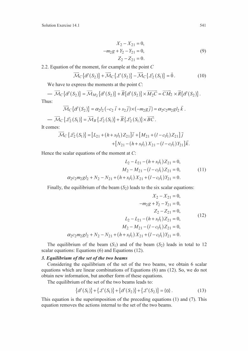
Solution Exercise 14.1 541
2 21
2 2 21
2 21
0,
0,
0.
X X
m g Y Y
Z Z
− =
− + − =
− =
(9)
2.2. Equation of the moment, for example at the point C
( ) ( ) ( ) 2 2 2 1 0C C CS S S+ − = . (10)
We have to express the moments at the point C:
( ) ( ) ( ) ( ) 2 22 2 2 2 2C MS S R S M C CM R S= + × = ×
.
Thus:
( ) ( ) ( ) 2 2 2 2 2 2 2 2 2 2C S l c i s j m g j c m gl kα α= − + × − = .
( ) ( ) ( ) 2 1 2 1 2 1C BS S R S BC= + ×
.
It comes:
( ) ( )[ ] ( )[ ]( ) ( )[ ]
2 1 21 1 1 21 21 1 1 21
21 1 1 21 1 1 21 .
C S L h s l Z i M l c l Z j
N h s l X l c l Y k
= + + + + −
+ − + − −
Hence the scalar equations of the moment at C:
( )
( )
( ) ( )
2 21 1 1 21
2 21 1 1 21
2 2 2 2 2 21 1 1 21 1 1 21
0,
0,
0.
L L h s l Z
M M l c l Z
c m gl N N h s l X l c l Yα
− − + =
− − − =
+ − + + + − =
(11)
Finally, the equilibrium of the beam (S2) leads to the six scalar equations:
( )
( )
( ) ( )
2 21
2 2 21
2 21
2 21 1 1 21
2 21 1 1 21
2 2 2 2 2 21 1 1 21 1 1 21
0,
0,
0,
0,
0,
0.
X X
m g Y Y
Z Z
L L h s l Z
M M l c l Z
c m gl N N h s l X l c l Yα
− =
− + − =
− =
− − + =
− − − =
+ − + + + − =
(12)
The equilibrium of the beam (S1) and of the beam (S2) leads in total to 12
scalar equations: Equations (6) and Equations (12).
3. Equilibrium of the set of the two beams
Considering the equilibrium of the set of the two beams, we obtain 6 scalar
equations which are linear combinations of Equations (6) ans (12). So, we do not
obtain new information, but another form of these equations.
The equilibrium of the set of the two beams leads to:
( ) ( ) ( ) ( ) 1 1 2 2 0S S S S+ + + = . (13)
This equation is the superimposition of the preceding equations (1) and (7). This
equation removes the actions internal to the set of the two beams.
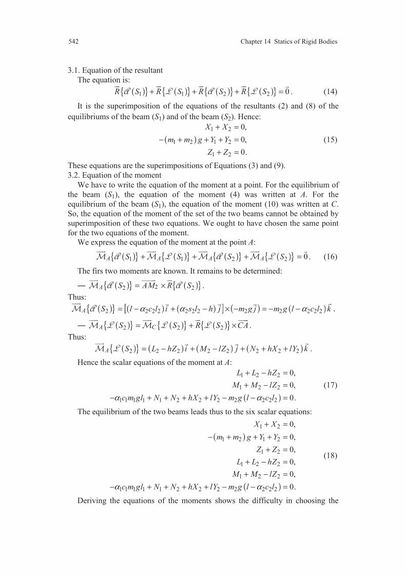
542 Chapter 14 Statics of Rigid Bodies
3.1. Equation of the resultant
The equation is:
( ) ( ) ( ) ( ) 1 1 2 2 0R S R S R S R S+ + + = . (14)
It is the superimposition of the equations of the resultants (2) and (8) of the
equilibriums of the beam (S1) and of the beam (S2). Hence:
( )1 2
1 2 1 2
1 2
0,
0,
0.
X X
m m g Y Y
Z Z
+ =
− + + + =
+ =
(15)
These equations are the superimpositions of Equations (3) and (9).
3.2. Equation of the moment
We have to write the equation of the moment at a point. For the equilibrium of
the beam (S1), the equation of the moment (4) was written at A. For the
equilibrium of the beam (S1), the equation of the moment (10) was written at C.
So, the equation of the moment of the set of the two beams cannot be obtained by
superimposition of these two equations. We ought to have chosen the same point
for the two equations of the moment.
We express the equation of the moment at the point A:
( ) ( ) ( ) ( ) 1 1 2 2 0A A A AS S S S+ + + = . (16)
The firs two moments are known. It remains to be determined:
( ) ( ) 22 2A S AM R S= ×
.
Thus:
( ) ( ) ( )[ ] ( ) ( )2 2 2 2 2 2 2 2 2 2 2 2A S l c l i s l h j m g j m g l c l kα α α= − + − × − = − − .
( ) ( ) ( ) 2 2 2A CS S R S CA= + ×
.
Thus:
( ) ( ) ( ) ( )2 2 2 2 2 2 2 2A S L hZ i M lZ j N hX lY k= − + − + + + .
Hence the scalar equations of the moment at A:
( )
1 2 2
1 2 2
1 1 1 1 1 2 2 2 2 2 2 2
0,
0,
0.
L L hZ
M M lZ
c m gl N N hX lY m g l c lα α
+ − =
+ − =
− + + + + − − =
(17)
The equilibrium of the two beams leads thus to the six scalar equations:
( )
( )
1 2
1 2 1 2
1 2
1 2 2
1 2 2
1 1 1 1 1 2 2 2 2 2 2 2
0,
0,
0,
0,
0,
0.
X X
m m g Y Y
Z Z
L L hZ
M M lZ
c m gl N N hX lY m g l c lα α
+ =
− + + + =
+ =
+ − =
+ − =
− + + + + − − =
(18)
Deriving the equations of the moments shows the difficulty in choosing the
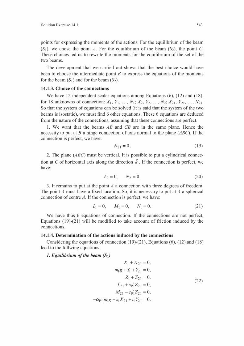
Solution Exercise 14.1 543
points for expressing the moments of the actions. For the equilibrium of the beam
(S1), we chose the point A. For the equilibrium of the beam (S2), the point C.
These choices led us to rewrite the moments for the equilibrium of the set of the
two beams.
The development that we carried out shows that the best choice would have
been to choose the intermediate point B to express the equations of the moments
for the beam (S1) and for the beam (S2).
14.1.3. Choice of the connections
We have 12 independent scalar equations among Equations (6), (12) and (18),
for 18 unknowns of connection: X1, Y1, …, N1; X2, Y2, …, N2; X21, Y21, …, N21.
So that the system of equations can be solved (it is said that the system of the two
beams is isostatic), we must find 6 other equations. These 6 equations are deduced
from the nature of the connections, assuming that these connections are perfect.
1. We want that the beams AB and CB are in the same plane. Hence the
necessity to put at B a hinge connection of axis normal to the plane (ABC). If the
connection is perfect, we have:
21 0N = . (19)
2. The plane (ABC) must be vertical. It is possible to put a cylindrical connec-
tion at C of horizontal axis along the direction k
. If the connection is perfect, we
have:
2 20, 0.Z N= = (20)
3. It remains to put at the point A a connection with three degrees of freedom.
The point A must have a fixed location. So, it is necessary to put at A a spherical
connection of centre A. If the connection is perfect, we have:
1 1 10, 0, 0.L M N= = = (21)
We have thus 6 equations of connection. If the connections are not perfect,
Equations (19)-(21) will be modified to take account of friction induced by the
connections.
14.1.4. Determination of the actions induced by the connections Considering the equations of connection (19)-(21), Equations (6), (12) and (18)
lead to the follwing equations.
1. Equilibrium of the beam (S1)
1 21
1 1 21
1 21
21 1 1 21
21 1 1 21
1 1 1 1 21 1 21
0,
0,
0,
0,
0,
0.
X X
m g Y Y
Z Z
L s l Z
M c l Z
c m g s X c Yα
+ =
− + + =
+ =
+ =
− =
− − + =
(22)
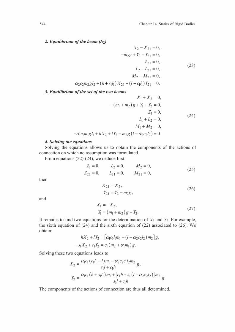
544 Chapter 14 Statics of Rigid Bodies
2. Equilibrium of the beam (S2)
( ) ( )
2 21
2 2 21
21
2 21
2 21
2 2 2 2 1 1 21 1 1 21
0,
0,
0,
0,
0,
0.
X X
m g Y Y
Z
L L
M M
c m gl h s l X l c l Yα
− =
− + − =
=
− =
− =
+ + + − =
(23)
3. Equilibrium of the set of the two beams
( )
( )
1 2
1 2 1 2
1
1 2
1 2
1 1 1 1 2 2 2 2 2 2
0,
0,
0,
0,
0,
0.
X X
m m g Y Y
Z
L L
M M
c m gl hX lY m g l c lα α
+ =
− + + + =
=
+ =
+ =
− + + − − =
(24)
4. Solving the equations
Solving the equations allows us to obtain the components of the actions of
connection on which no assumption was formulated.
From equations (22)-(24), we deduce first:
1 2 2
21 21 21
0, 0, 0,
0, 0, 0,
Z L M
Z L M
= = =
= = = (25)
then
21 2
21 2 2
,
,
X X
Y Y m g
=
= − (26)
and
( )1 2
1 1 2 2
,
.
X X
Y m m g Y
= −
= + − (27)
It remains to find two equations for the determination of X2 and Y2. For example,
the sixth equation of (24) and the sixth equation of (22) associated to (26). We
obtain:
( )[ ]( )
2 2 1 1 1 1 2 2 2 2
1 2 1 2 1 2 1 1
,
.
hX lY c l m l c l m g
s X c Y c m m g
α α
α
+ = + −
− + = +
Solving these two equations leads to:
( )
( ) ( )[ ]
1 1 1 1 1 2 2 1 2 22
1 1
1 1 1 1 1 1 1 2 2 2 22
1 1
,
.
c c l l m c c l mX g
s l c h
c h s l m c h s l c l mY g
s l c h
α α
α α
− −=
+
+ + + −=
+
The components of the actions of connection are thus all determined.

Solution Exercise 14.2 545
14.2 Equilibrium of a ladderThe analysis of the equilibrium of the person-ladder set is rather long and we
develop here only some elements.
To implement the analysis we choose a coordinate system (Oxyz) such as the
plane (Oxy) contains the plane of symmetry of the person-ladder set and such the
axis Oy
is upward vertical (Figure Exercise 14.2).
14.2.1. Mechanical actions
1. Actions exerted on the ladder (S)
1.1. Action of gravity, represented by the torsor ( ) e S :
( )
( )
e ,
e 0,Ge
R S Mg j
S
= −
=
where M is the mass of the ladder and eG its mass centre. If l is the length of the
ladder and α its inclination, the coordinates of eG are ( )cos , sin , 02 2l lα α .
1.2. Action exerted by the ground at A, represented by the torsor ( ) A S
We may describe this action as a force of which the support passes through the
point A. Thus:
( )
( )
,
0.
A A A A
A A
R S X i Y j Z k
S
= + +
=
Figure Exercise 14.2.
B
A
C
D
ground
wa
ll
G
y
O x
z
C
legD
arm
u

546 Chapter 14 Statics of Rigid Bodies
The components XA, YA and ZA are to be determined. Moreover, considering the
Coulomb’s law for dry friction (Chapter 13), equilibrium at A will occur only if:
sA AX f Y< ,
where fs is the coefficient of friction between the ladder and the ground.
1.3. Action exerted by the wall at B, represented by the torsor ( ) B S :
This action can also be described as a force of which the support passes
through the point B. Thus:
( )
( )
,
0.
B B B B
B B
R S X i Y j Z k
S
= + +
=
The components XB, YB and ZB are to be determined. As previously the law for the
dry friction implies that equilibrium at B occurs only if:
mB BX f Y< ,
where fm is the coefficient of dry friction between the ladder and the wall.
1.4. Action exerted by the person (P)
The problem for describing this action is complex, since this action depends on
the position of the person: support on the feet, assistance with the arms, etc.
We describe this action as the superimposition (Figure Exercise 14.2) of two
actions: one exerted at C, represented by the torsor ,C S→ and the other exerted
at D, represented by the torsor .D S→
1.4.1. Action exerted at C, represented by the torsor C S→
The action may be modelled as the action of a plane on a cylinder (Figure
Exercise 14.2). So:
,
.
C C C
C C C C
R C S X i Y j Z k
C S L i M j N k
→ = + +
→ = + +
Neglecting friction of spinning about the direction ,k
we shall have:
0CN = .
Such as to have equilibrium at C the components XC and YC they will have to
satisfy the conditions of friction between feet and ladder.
1.4.2. Action exerted at D, represented by the torsor D S→In the case where the person does not grip the rung at D, the action may be
modelled as a force of which the support is the axis of the arms (Figure Exercise
14.2) of direction u
. We have:
,
0.
D
D
R D S F u
D S
→ =
→ =
The direction u
is known.
2. Actions exerted on the person (P)
2.1. Action of gravity, represented by the torsor ( ) e P :
Solution Exercise 14.2 547
( )
( )
e ,
e 0,G
R P mg j
P
= −
=
where m is the mass of the person.
2.2. Action exerted by the ladder at the contact C, represented by the torsor
( ) C P :
( ) .C P C S= − →
2.3. Action exerted by the ladder at the point D, represented by the torsor
( ) D P :
( ) .D P D S= − →
14.2.2. Equilibrium person-ladder
The equilibrium of the ladder is written:
( ) ( ) ( ) e .0A BS S S C S D S+ + + =→ + →
The equilibrium of the person is written:
( ) e 0 .P C S D S− − =→ →
One of the two equations can be replaced by expressing the equilibrium of the
person-ladder set:
( ) ( ) ( ) ( ) e e .0A BS S S P+ + + =
This latter equation removes the actions internal to the person-ladder set.
We have thus 12 scalar equations to derive 12 components of the actions of
connection: XA, YA, ZA; XB, YB, ZB; XC, YC, ..., MC; FD.
The reader will solve easily these equations and will take account of the
conditions of friction at the points of contact A, B and D.

Chapter 15
The Operator of Inertia
15.1 Matrix of inertia of a rectangular plate (Figure 15.22)
The axes of the trihedron (Oxyz) being axes of symmetry of the plate, the
matrix of inertia at the centre O of the plate in the basis ( ) ( ), , b i j k=
is of the
form:
( )( )
0 0
0 0
0 0
Oxb
O Oy
Oz
I
S I
I
=
I ,
with from (15.41) and (15.42):
( )
( )
2
2
d ( ),
d ( ),
.
OxS
OyS
Oz Ox Oy
I y m M
I x m M
I I I
=
=
= +
Using the Cartesian coordinates, the mass of the element of plate is d ( )m M =
d ds x yρ , where sρ is the mass per unit surface of the plate. Hence:
2 2 2
2 2
d d
a b
Ox sa bx y
I y x yρ=− =−
= .
Thus: 3
2
12 12Ox s
b mI a bρ= = ,
where m is the mass of the plate. The moment OyI is obtained by changing the
roles of a and b. Hence the matrix of inertia:
( )( )
( )
2
2
2 2
0 012
0 012
0 012
bO
m b
mS a
m a b
= +
I .
It is the result (15.86).
15.2 Matrix of inertia of a quarter of disc
We choose the coordinate system (Oxyz) such as the axes Ox
and Oy
are along
the edges of the disc (Figure Exercise 15.2).
The matrix of inertia is of the form:

Solution Exercise 15.2 549
Figure Exercise 15.2.
( )( )
0
0
0 0
Ox Oxyb
O Oxy Oy
Oz
I P
S P I
I
− = −
I ,
with
( )
( )
( )( )
( )
2
2
2 2
d ( ),
d ( ),
d ( ),
d ( ).
OxS
OyS
Oz Ox OyS
OxyS
I y m M
I x m M
I I I x y m M
P xy m M
=
=
= + = +
=
The axes Ox
and Oy
play the same part. It follows that:
12
Ox Oy OzI I I= = .
To derive the moment of inertia OzI with respect to the axis Oz
, we use the polar
coordinates introduced in Figure 15.7. Hence:
2 2
0 0
d da
Oz sr
I r r r
π
αρ α
= == ,
where sρ is the mass per unit surface of the quarter of disc. Hence:
4 2
4 2 2Oz s
r aI mπρ= = ,
where m is the mass of the quarter of disc.
The product of inertia is:
y
O x
z
M
r
O x
z
y
()
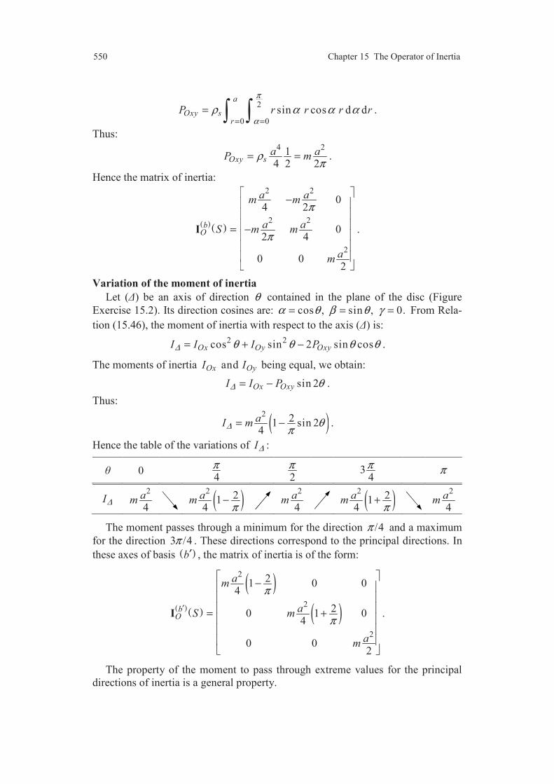
550 Chapter 15 The Operator of Inertia
2
0 0
sin cos d da
Oxy sr
P r r r r
π
αρ α α α
= == .
Thus: 4 21
4 2 2Oxy s
a aP mρπ
= = .
Hence the matrix of inertia:
( )( )
2 2
2 2
2
04 2
02 4
0 02
bO
a am m
a aS m m
am
π
π
−
= −
I .
Variation of the moment of inertia Let () be an axis of direction θ contained in the plane of the disc (Figure
Exercise 15.2). Its direction cosines are: cos , sin , 0.α θ β θ γ= = = From Rela-
tion (15.46), the moment of inertia with respect to the axis () is:
2 2cos sin 2 sin cosOx Oy OxyI I I P∆ θ θ θ θ= + − .
The moments of inertia and Ox OyI I being equal, we obtain:
sin 2Ox OxyI I P∆ θ= − .
Thus:
( )2 21 sin 2
4aI m∆ θ
π= − .
Hence the table of the variations of I∆ :
0 4π
2π 3
4π π
I∆2
4am ( )
2 214
amπ
−2
4am ( )
2 214
amπ
+2
4am
The moment passes through a minimum for the direction /4π and a maximum
for the direction 3 /4π . These directions correspond to the principal directions. In
these axes of basis ( )b′ , the matrix of inertia is of the form:
( )( )
( )( )
2
2
2
21 0 04
20 1 04
0 02
bO
am
aS m
am
π
π′
−
= +
I .
The property of the moment to pass through extreme values for the principal
directions of inertia is a general property.

Solution Exercise 15.3 551
15.3 Matrix of inertia of a hollowed cylinder We consider the hollowed cylinder (S) (Figure Exercise 15.3) of inner radius
a1, of outer radius a2 and height h.
The solid cylinder (S2) of radius a2 can be considered as the union of the hollo-
wed cylinder (S) and of the cylinder (S1) of radius a1 which was removed. The
property of associativity of the matrices of inertia is written:
( )( ) ( )( ) ( )( )2 1b b b
O O OS S S=I I + I .
Hence the matrix of inertia of the hollowed cylinder:
( )( ) ( )( ) ( )( )2 1b b b
O O OS S S= −I I I .
The matrix of inertia of the cylinder (S1) is, from (15.101):
( )( )
2 21
1
2 21
1 1
21
1
0 04 3
0 04 3
0 02
bO
a hm
a hS m
am
+
= +
I ,
where the mass m1 of the cylinder (S1) is: 2
1 1m a hπ ρ= ,
introducing the mass per unit volume of the cylinder.
Figure Exercise 15.3.
y
x
z
a2 a1
O
h
(S)

552 Chapter 15 The Operator of Inertia
The matrix of inertia of the cylinder (S2) is similarly:
( )( )
2 22
2
2 22
2 2
22
2
0 04 3
0 04 3
0 02
bO
a hm
a hS m
am
+
= +
I ,
where the mass m2 of the cylinder (S2) is: 2
2 2m a hπ ρ= .
The mass of the hollowed cylinder is:
( )2 22 1 2 1m m m a a hπ ρ= − = − .
From the expressions of the masses m, m1 and m2, we deduce:
2 21 2
1 22 2 2 22 1 2 1
, .a a
m m m ma a a a
= =− −
The application of the relation between the matrices of inertia leads to:
( )( )0 0
0 0
0 0
Oxb
O Oy
Oz
I
S I
I
=
I ,
with:
( )
( )
2 22 2
22 2
1 ,4 3
1 ,2
Ox Oy a
Oz a
a hI I m r
aI m r
= = + +
= +
introducing the radius ratio: 1
2a
ar
a= .
In the case of a hollowed cylinder of low thickness, we have 1 2a a a≈ ≈ and
the moments of inertia are written: 2 2
2
,2 3
.
Ox Oy
Oz
a hI I m
I ma
= = +
=
15.4 Matrix of inertia of a solid (Figure 15.23)
The solid is constituted of a cylinder (S1) of radius a and height h and of a half-
sphere (S2) of radius a.
The mass of the cylinder is:
21m a hπ ρ= ,
where ρ is the mass per unit volume of the solid. Its matrix of inertia in the
basis ( )b = ( ), , i j k
is:
Solution Exercise 15.5 553
( )( )
2 2
1
2 2
1 1
2
1
0 04 3
0 04 3
0 02
bO
a hm
a hS m
am
+
= +
I .
The mass of the half-sphere is 32
23
m aπ ρ= and its matrix of inertia at the
point O in the basis (b) is:
( )( )
22
22 2
22
20 0
52
0 05
20 0
5
bO
m a
S m a
m a
=
I .
The mass of the set cylinder and half-sphere is:
( )21 2
23
m m m a a hπ ρ= + = + .
From the expressions of the masses m1, m2 and m, we deduce:
1 2
23, .
2 23 3
ahm m m m
a h a h= =
+ +
The matrix of inertia of the set is diagonal and the diagonal terms are expressed
as:
( )2
2
1 42 2 15 ,
23
415 ,23
Ox Oy
Oz
rrI I ma
r
rI ma
r
+ += =
+
+=
+
Introducing the ratio: /r h a= .
15.5 Matrix of inertia of a non homogeneous parallelepiped (Figure
15.24)
The parallelepiped (S) is constituted (Figure Exercise 15.5) of four parallele-
pipeds (S1), (S2), (S3) and (S4).
The parallelepiped (S1) has a mass m1 and its mass centre G1 has for coordi-
nates ( )0, , 2 2b c− . Its matrix of inertia at G1 in the basis ( ) ( ), , b i j k=
is from
(15.103):

554 Chapter 15 The Operator of Inertia
( )( )
( )
( )
( )
1
2 21
2 211
2 21
0 012
0 4 012
0 0 412
bG
mb c
mS a c
ma b
+ = +
+
I .
The parallelepiped (S2) has a mass m2 and its mass centre G2 has for coordi-
nates ( )0, , 2 2b c . Its matrix of inertia at G2 is similarly:
( )( )
( )
( )
( )
2
2 22
2 222
2 22
0 012
0 4 012
0 0 412
bG
mb c
mS a c
ma b
+ = +
+
I .
The parallelepiped (S3) has a mass m1 and its mass centre G3 has for coordi-
nates ( )0, , 2 2b c− . Its matrix of inertia is equal to the one of (S1):
( )( ) ( )( )3 1
3 1b b
G GS S=I I .
The parallelepiped (S4) has a mass m2 and its mass centre G4 has for coordi-
nates ( )0, , 2 2b c− − . Its matrix of inertia is equal to the one of (S2):
( )( ) ( )( )4 2
4 2b b
G GS S=I I .
The parallelepiped (S) constituted of the four parallelepipeds has a matrix of
inertia at O expressed by:
( )( ) ( )( ) ( )( ) ( )( ) ( )( )1 2 3 4b b b b b
O O O O OS S S S S+ +I = I I I + I .
Figure Exercise 15.5.
2c
y
x
z
2a
2b
Om1
m1 m2
m2
(S1)
(S2)
(S3) (S4)
()
A

Solution Exercise 15.5 555
We have thus to express the matrices of inertia of each parallelepiped at point O.
For the parallelepiped (S1), we have:
( )( ) ( )( ) ( ) ( )1 1
1 1 1b b b
O G OGS S S=I I + D ,
with from Relation (15.24):
( ) ( )
( )( )
( )
1 1 1 11 1
1 1 1 11 1 1
1 1 1 1 1 1
2 21 1 1
2 21 1 1 1
2 21 1 1
G G G GG G
bG G G GOG G G
G G G G G G
m y z m x y m x z
S m x y m x z m y z
m x z m y z m x y
+ − − = − + −
− − +
D ,
where 1 1 1, and G G Gx y z are the coordinates of the mass centre G1. Hence:
( ) ( )
( )
1
2 21
21 11
21 1
0 04
04 4
04 4
bOG
mb c
m mS c bc
m mbc b
+ =
D .
The matrix of inertia at O is thus:
( )( )
( )
( )
( )
2 21
2 21 11
2 21 1
0 03
03 4
04 3
bO
mb c
m mS a c bc
m mbc a b
+ = +
+
I .
For the parallelepiped (S2), we have:
( )( ) ( )( ) ( ) ( )2 2
2 2 2b b b
O G OGS S S=I I + D ,
where the coordinates of the mass centre are ( )0, , 2 2b c . With the same process
as previously, we obtain:
( )( )
( )
( )
( )
2 22
2 22 22
2 22 2
0 03
03 4
04 3
bO
mb c
m mS a c bc
m mbc a b
+ = + −
− +
I .
Applying the preceding relations to the parallelepipeds (S3) and (S4), we find that: ( )( ) ( )( ) ( )( ) ( )( )3 1 4 2 et b b b bO O O OS S S S= =I I I I .
Hence the matrix of inertia:

556 Chapter 15 The Operator of Inertia
( )( )
( )( )
( )( ) ( )
( ) ( )( )
2 21 2
2 21 2 1 2
2 21 2 1 2
20 0
32 1
03 2
1 20
2 3
bO
m m b c
S m m a c m m bc
m m bc m m a b
+ +
= + + − − − − + +
I
Moment of inertia with respect to a diagonal of the parallelepipedLet () be the diagonal passing through the vertex A of the parallelepiped. The
vector OA
is a direction vector of the axis ():
OA a i b j c k= + +
.
The direction cosines of the axis are thus:
2 2 2 2 2 2 2 2 2, , .a b c
a b c a b c a b cα β γ= = =
+ + + + + +
The moment of inertia with respect to () is deduced from Relation (15.46). Thus:
2 2 2 2Ox Oy Oz OyzI I I I P∆ α β γ βγ= + + − .
That leads to:
( )( ) ( )2 2 2 2 2 2 2 21 2 1 22 2 2
1 43
I m m a b b c a c m m b ca b c
∆ = + + + − − + +
.
15.6 Matrix of inertia of a solid sphere with a spherical holeA solid sphere (S) of radius a contains a spherical hole of radius /2a , passing
through the centre of the solid sphere (Figure Exercise 15.6). The solid sphere (S1)
can be considered as constituted of the hollowed sphere (S) and of the solid sphere
(S2) which was removed. The property of associativity of the matrices of inertia is
written: ( )( ) ( )( ) ( )( )1 2b b b
O O OS S S=I I + I
Figure Exercise 15.6.
y
z
x
O G2
(S2)
(S1)
Solution Exercise 15.6 557
Hence the matrix of inertia of the hollowed sphere:
( )( ) ( )( ) ( )( )1 2b b b
O O OS S S= −I I I .
The matrix of inertia of the solid sphere (S1) is:
( )( )
21
21 1
21
20 0
52
0 05
20 0
5
bO
m a
S m a
m a
=
I ,
where m1 is the mass of the solid sphere (S1).
The matrix of inertia of the solid sphere (S2) at the mass centre G2 is:
( )( )2
22
222
22
0 010
0 010
0 010
bG
ma
mS a
ma
=
I ,
where m2 is the mass of the solid sphere (S2). This matrix has to be evaluated at
the point O. Thus: ( )( ) ( )( ) ( ) ( )
2 22 2 2
b b bO G OG
S S S=I I + D ,
where the coordinates of the point G2 are ( )0, , 02a . Hence:
( ) ( )2
22
2
22
0 04
0 0 0
0 04
bOG
ma
S
ma
=
D .
Thus:
( )( )
22
222
22
70 0
20
0 010
70 0
20
bO
m a
mS a
m a
=
I .
So, we deduce the expression of the matrix of inertia of the hollowed sphere:
( )( )
( )( )
( )
21 2
221
21 2
2 70 0
5 202
0 05 10
2 70 0
5 20
bO
m m a
mS m a
m m a
−
= − −
I .

558 Chapter 15 The Operator of Inertia
The radius of the removed sphere (S2) is half the radius of the sphere (S1). It
follows that 2 1/8m m= . That leads to:
1 28 , .7 7
mm m m= =
where m is the mass of the hollowed sphere (S).
Finally the matrix of inertia is written as:
( )( )
2
2
2
570 0
14031
0 070
570 0
140
bO
ma
S ma
ma
=
I .
15.7 Matrix of inertia of a plate with a hole (Figure Exercise 15.7)
The reader will find easily that the matrix of inertia of the plate (S) with a
circular hole is:
( )( )
2 2
2 2
2 2 2
0 01 12 4
0 01 12 4
0 01 12 2
cc
bO c
c
cc
m b cr
r
m a cS r
r
m a b cr
r
− −
= − −
+ − −
I ,
introducing the mass m of the plate with the hole and the ratio of surfaces: 2
ccr
abπ= .
Figure Exercise 15.7.
y
xb
a
O
c
z

Chapter 16
Kinetic and Dynamic Torsors
Kinetic Energy
16.1 Motion of rotation of a parallelepiped about an axis passing through its centre (Figure 16.2a)
The study of the motion will be always implemented according to the same
process: 1) determination of the parameters of situation, 2) kinematic study, 3)
kinetic study.
1. Parameters of situation We associate a coordinate system attached to the reference (T) of the motion:
the system (Oxyz) (Figure Exercise 16.1) such as the axis Oz
coincides with the
axis of rotation and such as the point O coincides with the centre of the paralle-
lepiped. The axis Ox
is chosen along a given direction of the plane (Oxy).
1.1. Parameters of translation
We choose a particular point of the parallelepiped (S): the point O. This point
is fixed during the motion. So, there is no parameter of translation.
1.2. Parameters of rotation
We associate a trihedron attached to the parallelepiped: the trihedron ( )S SOx y z
such as the axes SOx
and SOy
are parallel to the edges. We have a rotation of
Figure Exercise 16.1.
y
z
x
(T)
O
yS
xS
(S)
()

560 Chapter 16 Kinetic and Dynamic Torsors. Kinetic Energy
angle about the direction k
. Thus, one parameter of rotation .
The basis change is:
cos sin ,
sin cos ,
.
S
S
i i j
j i j
k
ψ ψ
ψ ψ
= +
= − +
2. Kinematic study
The kinematic torsor( ) TS relative to the motion of the parallelepiped (S) with
respect to the reference (T) has for elements of reduction at the point O:
( ) ( )
( ) ( )
, instantaneous rotation vector relative to the motion,
( , ) 0, velocity vector of the particular point .
T TS S
T TO S
R k
O t O
ω ψ = =
= =
3. Kinetic study 3.1. Kinetic torsor
The kinetic torsor ( ) T
S relative to the motion of the parallelepiped (S) with
respect to the reference (T) has for elements of reduction at the point point O,
which is the mass centre of the parallelepiped:
( ) ( )
( ) ( ) ( )
( , ) 0,
, since is the mass centre.
T TS
T TO S O S
R m O t
S Oω
= =
=
The operator of inertia ( )O S of the parallelepiped at the point O is represented
in the basis ( ) ( ), , S S Sb i j k=
by the matrix of inertia expressed in the preceding
chapter:
( )( )
( )
( )
( )
2 2
2 2
2 2
0 012
0 012
0 012
SbO
m b c
mS a c
m a b
+
= + +
I ,
where m is the mass, and a, b, c are the edges of the parallelepiped. We have to
note that the matrices of inertia were evaluated in the preceding chapter in a basis
attached to the solids. Hence the use here of the basis ( )Sb .
It results that: ( )
( ) ( )
2 2
0,
,12
TS
TO S
R
ma b k C kψ ψ
=
= + =
setting:
( )2 2
12
mC a b= + .
3.2. Kinetic energy
The expression of the kinetic energy is:
Solution Exercise 16.2 561
( ) ( ) ( ) c1( )2
T T TS SE S = ⋅ .
To derive the product of the torsors, we implement the sum of the crossed scalar
products of the resultants and moments of the torsors expressed at the same point.
Here:
( ) ( ) ( ) ( ) ( ) c1( )2
T T T T TO OS S S SE S R R = + ⋅ ⋅
.
Hence:
( ) ( )2 2 2 2c
1( )24 2
T mE S a b Cψ ψ= + = .
3.3. Dynamic torsor
The dynamic torsor ( ) TS relative to the motion of the parallelepiped (S) with
respect to the reference (T) has for elements of reduction at the point O:
( ) ( )
( ) ( ) ( ) ( ) ( ) ( )
( , ) ,
.
T TS
T T T TO S O S S O S
R ma O t
S Sω ω ω
=
= + ×
The vector ( )TSω is expressed by kψ
. The vector product is null, since the two
vectors are collinear. Hence:
( ) ( ) ( )
2 2
0,
.12
TS
TO S
R
ma b k C kψ ψ
=
= + =
We observe that the expression of the moment of the dynamic torsor could
have been got by deriving the expression of the moment at O of the kinetic torsor
(Property (16.24)). If this property is interesting in the present case, it is not
recommended to use this property in a general way.
16.2 Motion of rotation of a parallelepiped about an eccentric axis (Figure 16.2b)
The analysis is implemented according the same process as the one used in the
preceding exercise.
1. Parameters of situation We associate a coordinate system attached to the reference (T) of the motion:
the system (Oxyz) (Figure Exercise 16.2) such as the axis Oz
coincides with the
axis of rotation and such as the point O is located in the medium plane of the
parallelepiped. The axis Ox
is chosen along a given direction of the medium plane.
1.1. Parameters of translation
We choose a particular point of the parallelepiped (S): the point O. This point
is fixed during the motion. So, there is no parameter of translation.
1.2. Parameters of rotation
We associate a coordinate system attached to the parallelepiped: the system
( )S SOx y z such as the axes SOx
and SOy
are parallel to the edges. We have a
rotation of angle about the direction k
. Hence one parameter of rotation .

562 Chapter 16 Kinetic and Dynamic Torsors. Kinetic Energy
Figure Exercise 16.2.
The basis change is:
cos sin ,
sin cos ,
.
S
S
i i j
j i j
k
ψ ψ
ψ ψ
= +
= − +
2. Kinematic study 2.1. Kinematic torsor
The kinematic torsor( ) TS relative to the motion of the parallelepiped (S) with
respect to the reference (T) has for elements of reduction at O:
( ) ( )
( ) ( )
, instantaneous rotation vector relative to the motion,
( , ) 0, velocity vector of the particular point .
T TS S
T TO S
R k
O t O
ω ψ = =
= =
2.2. Kinematic vectors of the mass centre
The velocity and acceleration vectors of the mass centre are needed for deri-
ving the resultants of the kinetic and dynamic torsors.
The velocity vector can be deduced while writing the expression of the moment
at the point G of the kinematic torsor:
( ) ( ) ( ) T T TG OS S SR OG= + ×
.
That leads to the relation between the velocity vectors:
( ) ( ) ( ) ( , ) ( , )T T T
SG t O t OGω= + ×
,
with:
y
z
x
(T)
O
yS
xS
(S)
()
d
G
Solution Exercise 16.2 563
( )2S S
aOG d i l i= − =
,
where a is the length of the edge of the parallelepiped and setting:
2al d= − .
Hence: ( )
( , )TSG t l jψ= .
The velocity vector can also be obtained from the relation of the definition of
the velocity vector:
( )( )
d( , )
d
TT G t OG
t=
,
where OG
was expressed previously. We thus obtain directly the preceding
expression for the velocity vector.
The acceleration vector is obtained by deriving the velocity vector with respect
to time and considering that ψ and Sj
are functions of time. We thus obtain:
( ) ( )2( , )TS Sa G t l i jψ ψ= − +
.
The kinematic vectors can be eventually expressed in the basis ( ), , i j k
intro-
ducing the relation of basis change. Hence: ( ) ( )( , ) sin cosT G t l i jψ ψ ψ= − +
,
( ) ( ) ( )2 2( , ) cos sin sin cosTa G t l i jψ ψ ψ ψ ψ ψ ψ ψ = − + + − +
.
3. Kinetic study 3.1. Kinetic torsor
The kinetic torsor ( ) T
S relative to the motion of the parallelepiped (S) with
respect to the reference (T) has for elements of reduction at the point O:
( ) ( )
( ) ( ) ( ) ( )
( , ) ,
( , ) .
T TS S
T T TO S O S
R m G t ml j
m OG O t S
ψ
ω
= =
= × +
The velocity vector of the point O being null, the first term of the moment is null.
The operator of inertia ( )O S of the parallelepiped at the point O is represented in
the basis ( ) ( ), , S S Sb i j k=
by the matrix of inertia at G as:
( )( ) ( )( ) ( )( )S S Sb b bO G OGS S S=I I + D .
The coordinates of the point G relatively to the system ( )S SOx y z being (l, 0, 0),
we have:
( )( ) 2
2
0 0 0
0 0
0 0
SbOG S ml
ml
=
D .
Hence the matrix of inertia at O:

564 Chapter 16 Kinetic and Dynamic Torsors. Kinetic Energy
( )( )
( )2 2
2 22
2 22
0 012
0 012
0 012
SbO
m b c
a cS m l
a bm l
+ += +
+ +
I .
Finally we obtain: ( )
( ) ( )2
,
.
TS S
TO S
R ml j
C ml k
ψ
ψ
=
= +
3.2. Kinetic energy
The kinetic energy is expressed as:
( ) ( ) ( ) c1( )2
T T TS SE S = ⋅ .
We have to implement the crossed scalar products of the resultants and moments
of the torsors expressed at the point O. we obtain:
( ) ( )2 2c
1( )2
TE S C ml ψ= + .
3.3. Dynamic torsor
The dynamic torsor ( ) TS relative to the motion of the parallelepiped (S) with
respect to the reference (T) has for elements of reduction at the point O:
( ) ( ) ( )( ) ( ) ( ) ( ) ( ) ( ) ( )
2 ( , ) ,
( , ) .
T TS S S
T T T T TO S O S S O S
R ma G t ml i j
m OG a O t S S
ψ ψ
ω ω ω
= = − +
= × + + ×
The first term of the moment is null since the point O is fixed. In the third term,
the two vectors are collinear to k
. Their vector product is thus null. Hence:
( ) ( )( ) ( )
2
2
,
.
TS S S
TO S
R ml i j
C ml k
ψ ψ
ψ
= − +
= +
16.3 Motion of a parallelepiped on a plane (Figure 16.3)
This motion was studied before in Exercise 9.1. We consider again the ele-
ments introduced.
1. Parameters of situation
We associate (Figure Exercise 16.3) the coordinate system (Oxyz) to the plane
(T) on which the parallelepiped moves, such as the plane (Oxy) coincides with the
plane (T). The axis Ox
is chosen along a given direction of the plane.
1.1. Parameters of translation
We choose a particular point of the parallelepiped (S). In Exercise 9.1, we
chose the point A vertex of the parallelepiped. However, it is possible to choose

Solution Exercise 16.3 565
Figure Exercise 16.3.
the mass centre G, that will simplify the kinetic analysis. The coordinates of G are
( ), , /2x y c where c is the height of the parallelepiped. We have two parameters
of translation: x and y.
1.2. Parameters of rotation
We associate the coordinate system ( )S SGx y z attached to the parallelepiped,
such as the axes SGx
and SGy
are parallel to the edges. The orientation is given
by the rotation about the direction k
. Hence:
cos sin ,
sin cos ,
.
S
S
i i j
j i j
k
ψ ψ
ψ ψ
= +
= − +
2. Kinematic study 2.1. Kinematic torsor
The kinematic torsor( ) TS relative to the motion of the parallelepiped (S) with
respect to the plane (T) has for elements of reduction at G:
( ) ( )
( ) ( )
, instantaneous rotation vector relative to the motion,
( , ) , velocity vector of the point .
T TS S
T TG S
R k
G t x i y j G
ω ψ = =
= = +
2.2. Acceleration vector of the mass centre
The vector is:
( )( )
( )
d( , ) ( , )
d
TT Ta G t G t x i y j
t= = +
.
3. Kinetic study 3.1. Kinetic torsor
The kinetic torsor ( ) T
S relative to the motion has for elements of reduction
at the point G:
(T) (S) A
B
C
D A'
B'
C'
D'
O
x
x
xS
yS
y z z
ijk
Si
Sj G
566 Chapter 16 Kinetic and Dynamic Torsors. Kinetic Energy
( ) ( ) ( )( ) ( ) ( ) ( )
2 2
( , ) ,
.12
T TS
T TG S G S
R m G t m x i y j
mS a b k C kω ψ ψ
= = +
= = + =
3.2. Kinetic energy
The kinetic energy is expressed by:
( ) ( ) ( ) c1( )2
T T TS SE S = ⋅ .
Thus, expressing the crossed scalar products of the resultants and moments at the
point G, we obtain:
( ) ( )2 2 2c
1 1( )2 2
TE S m x y Cψ= + + .
The first term is the kinetic energy of translation and the second term is the kinetic
energy of rotation.
3.3. Dynamic torsor
The dynamic torsor ( ) TS relative to the motion has for elements of reduction
at the point G:
( ) ( ) ( )( ) ( ) ( ) ( ) ( ) ( )
( , ) ,
.
T TS
T T T TG S G S S G S
R ma G t m x i y j
S S C kω ω ω ψ
= = +
= + × =
The three exercises 16.1, 16.2 and 16.3 allow us to underline the differences
between three motions of a same solid.

Chapter 21
Dynamics of Systems with One Degree of Freedom
Analysis of Vibrations
21.1 Mass drived by a wheel (Figure 21.15)
1. Equation of motion of the mass when the wheel is motionless We consider first the case where the point A of the axle-tree is fixed (Figure
Exercise 21.1). At the equilibrium the mass centre of the mass m coincides with
O. The actions exerted on the mass are: the gravity, the action of the spring and
the viscous friction. Hence the equation of motion:
my mg ky cy= − − − .
The position of equilibrium of the mass ( 0, 0y y= = ) is:
stmg
yk
= − .
With the given values, we obtain: st 5.2 mm.y = −
Around this position of equilibrium, the equation of motion is:
0my cy ky+ + = ,
or
202 0y y yδ ω+ + = ,
where δ is the damping coefficient and the natural angular frequency is
0 /k mω = , thus 0 43.3 rad/sω = .
2. Equation of motion when the wheel moves On account of the undulated surface, the centre A of the wheel has a motion
defined by the equation sin /Ay d x lπ= . Considering that at the origin instant
0t = , the point of contact of the wheel is at 0x = , and introducing the distance
covered at the instant t: x t= , the displacement of the centre of the wheel is:
sinAy d tω= ,
where the angular frequency ω is given by /lω π= , being the speed of the
wheel.
Figure Exercise 21.1.
k
m
A
y
OG
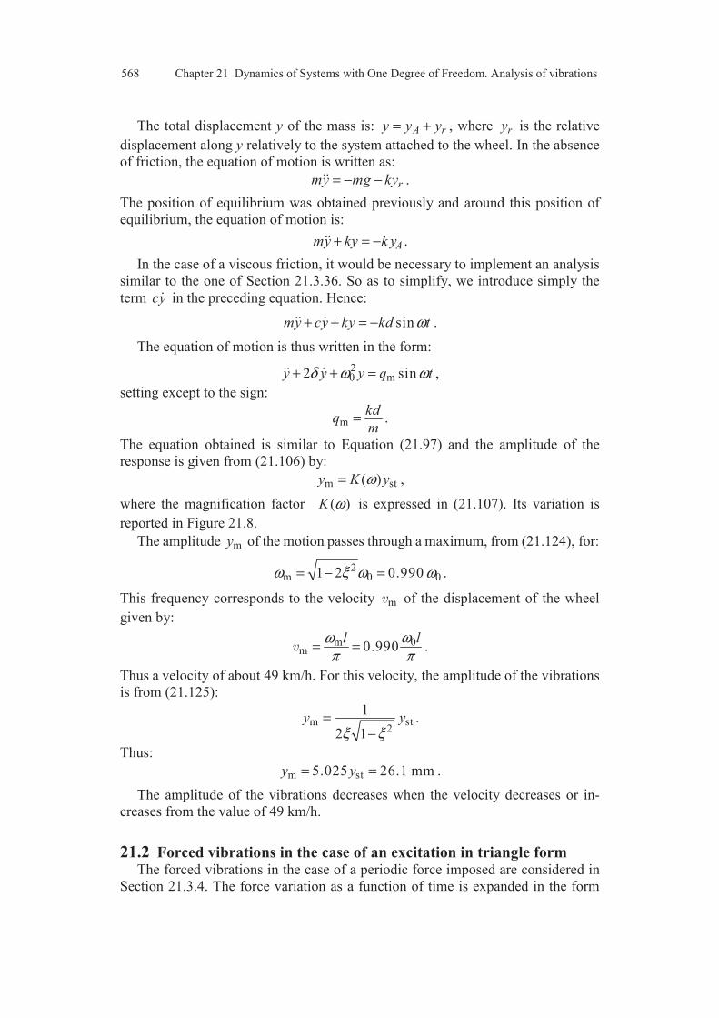
568 Chapter 21 Dynamics of Systems with One Degree of Freedom. Analysis of vibrations
The total displacement y of the mass is: A ry y y= + , where ry is the relative
displacement along y relatively to the system attached to the wheel. In the absence
of friction, the equation of motion is written as:
rmy mg ky= − − .
The position of equilibrium was obtained previously and around this position of
equilibrium, the equation of motion is:
Amy ky k y+ = − .
In the case of a viscous friction, it would be necessary to implement an analysis
similar to the one of Section 21.3.36. So as to simplify, we introduce simply the
term cy in the preceding equation. Hence:
sinmy cy ky kd tω+ + = − .
The equation of motion is thus written in the form:
20 m2 siny y y q tδ ω ω+ + = ,
setting except to the sign:
mkd
qm
= .
The equation obtained is similar to Equation (21.97) and the amplitude of the
response is given from (21.106) by:
m st( )y K yω= ,
where the magnification factor ( )K ω is expressed in (21.107). Its variation is
reported in Figure 21.8.
The amplitude my of the motion passes through a maximum, from (21.124), for:
2m 0 01 2 0.990ω ξ ω ω= − = .
This frequency corresponds to the velocity m of the displacement of the wheel
given by:
0mm 0.990
ll ωωπ π
= = .
Thus a velocity of about 49 km/h. For this velocity, the amplitude of the vibrations
is from (21.125):
m st2
1
2 1y y
ξ ξ=
−.
Thus:
m st5.025 26.1 mmy y= = .
The amplitude of the vibrations decreases when the velocity decreases or in-
creases from the value of 49 km/h.
21.2 Forced vibrations in the case of an excitation in triangle form The forced vibrations in the case of a periodic force imposed are considered in
Section 21.3.4. The force variation as a function of time is expanded in the form

Solution Exercise 21.2 569
of Fourier series (21.134) of which the coefficients are given by Expressions
(21.135)-(21.137).
In the case of the variation in triangle form of Figure 21.16, the function ( )f t
is antisymmmetric with respect to /2t T= . Hence:
/2
0 /2
( ) d ( ) dT T
T
f t t f t t= − .
It follows that the term a0 given by (21.135) is zero.
The term an is expressed by (21.136). The function cos n tω is symmetric with
respect to /2t T= . Associated to the antisymmetry of ( )f t , this symmetry leads to:
/2
0 /2
( ) cos d ( )cos dT T
T
f t n t t f t n t tω ω= − .
The terms an are thus zero.
The term bn is given by Expression (21.137). In the interval from 0 to /2T , the
function ( )f t is symmetric with respect to /4T , and in the interval from /2T to T,
the function is symmetric with respect to 3 /4T . Furthermore, when n is even, the
corresponding parts of the function sin n tω are antisymmetric. It follows that the
terms bn are zero for 2, 4, etc.n =
When n is odd, the function ( )f t and sin n tω are antisymmetric with respect to /2T . It results that Expression (21.137) leads to:
/4
0 0
2 8( )sin d ( )sin d
T T
nb f t n t t f t n t tT T
ω ω= = .
In the interval from 0 to /4T , we have:
4( )
Af t t
T= ,
and the expression of bn becomes: /4
20
32sin d
T
nA
b t n t tT
ω= .
For the integration, we introduce the change of variable: 2
u n t n tT
πω= = . Hence:
2
2 20
8sin d
n
nA
b u u un
π
π= .
Integrating by part, we obtain:
1
22 2 2 2
8 8sin ( 1) , 1, 3, 5, . . .
2
n
nA A
b n nn n
π
π π
−
= = − =
Hence:
( )2
8 1 1( ) sin sin 3 sin 5 . . .
9 25
Af t t t tω ω ω
π= − + − .
We observe that the series converges rapidly. It results that the force in triangle
570 Chapter 21 Dynamics of Systems with One Degree of Freedom. Analysis of vibrations
form produces approximatively the same effect as a sinusodal force of period T
expressed by:
2
8( ) sin
Af t tω
π= .
So as to consider the importance of the second term of the series, we can
evaluate the magnification factor ( )K ω given by Expression (21.107). At the
resonance ( 0ω ω= ), the magnification factor for the first term is:
1 01
( )2
K ωξ
= ,
And for the second term, we have:
3 02
1 1( )
9 4 36K ω
ξ=
+.
If 0.10ξ = , we obtain:
1 0 3 0( ) 5, ( ) 0.053,K Kω ω= =
thus an error of about 1 % while considering only the first term.
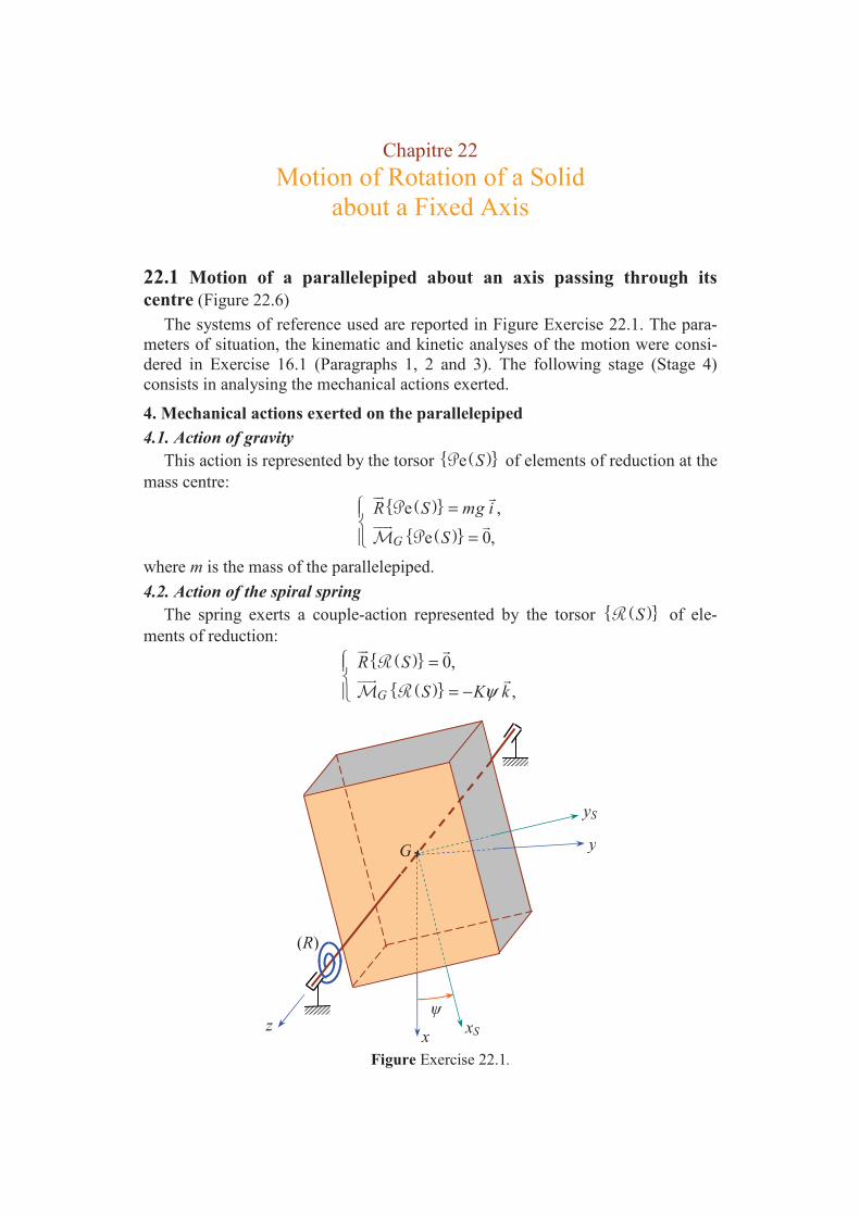
Chapitre 22
Motion of Rotation of a Solid
about a Fixed Axis
22.1 Motion of a parallelepiped about an axis passing through its centre (Figure 22.6)
The systems of reference used are reported in Figure Exercise 22.1. The para-
meters of situation, the kinematic and kinetic analyses of the motion were consi-
dered in Exercise 16.1 (Paragraphs 1, 2 and 3). The following stage (Stage 4)
consists in analysing the mechanical actions exerted.
4. Mechanical actions exerted on the parallelepiped
4.1. Action of gravity
This action is represented by the torsor ( ) e S of elements of reduction at the
mass centre:
( )
( )
e ,
e 0,G
R S mg i
S
=
=
where m is the mass of the parallelepiped.
4.2. Action of the spiral spring
The spring exerts a couple-action represented by the torsor ( ) S of ele-
ments of reduction:
( )
( )
0,
,G
R S
S K kψ
=
= −
Figure Exercise 22.1.
G
(R)
xxS
yS
y
z

572 Chapter 22 Motion of Rotation of a Solid about a Fixed Axis
wher K is the constant of torsion and the angle ψ is measured from the position
where the spring does not exert any action on the solid.
4.3. Action of the support induced by the hinge connection
This action is represented by the torsor ( ) S of elements of reduction at the
point G:
( )
( )
,
.
l l l
G l l l
R S X i Y j Z k
S L i M j N k
= + +
= + +
The components Xl, Yl, . . . , Nl are to be determined.
The power developed by the action is: ( ) ( ) ( ) ( ) T T
SP S S= ⋅ ,
where the kinematic torsor was expressed in Paragraph 2 of the correct version of
Exercice 16.1. We then obtain: ( ) ( ) T
lP S N ψ= .
5. Fundamental relation of dynamics
The relation is: ( ) ( ) ( ) ( ) e ,TS S S S= + +
where the dynamic torsor was expressed in Paragraph 3 of the correct version of
Exercice 16.1. We obtain the six scalar equations:
resultant:
0 ,
0 ,
0 ,
l
l
l
mg X
Y
Z
= +
=
=
moment at G:
0 ,
0 ,
.
l
l
l
L
M
C N Kψ ψ
=
=
= −
The first five equations give the components of the actions of connection:
, 0, 0, 0, 0.l l l l lX mg Y Z L M= − = = = =
The last equation is the equation of motion:
.lC N Kψ ψ= −
For solving the equation, it is necessary to introduce an assumption on the physic-
cal nature of the hinge connection: with friction or without friction.
In the case where there is no friction, the power developed is zero. Thus:
( ) ( ) 0TlP S N ψ= = .
That leads to 0.lN = The equation of motion is thus written as:
20 0ψ ω ψ+ = ,

Solution Exercise 21.2 573
setting:
( )20 2 2
12K KC m a b
ω = =+
.
In the case of a hinge connection with friction of viscous type, the component
lN is opposed to the angular velocity of rotation:
lN cψ= − ,
and the equation of motion is written in the form:
202 0ψ δψ ω ψ+ + = ,
setting:
( )2 2
62c cC m a b
δ = =+
.
The equations of motion obtained are the ones of a motion with one degree of
freedom (Chapter 21) with friction or without friction.
22.2 Motion of a parallelepiped about an eccentric axis (Figure 22.7a)
The reference systems used are reported in Figure Exercise 22.2. The para-
meters of situation, the kinematic and kinetic analyses of the motion were
considered in Exercise 16.1 (Paragraphs 1, 2 and 3). The following stage (Stage 4)
consists in analysing the mechanical actions exerted.
4. Mechanical actions exerted on the parallelepiped
4.1. Action of gravity
This action is represented by the torsor ( ) e S of elements of reduction at
Figure Exercise 22.2.
G
Od
x xS
yS
y
z
574 Chapter 22 Motion of Rotation of a Solid about a Fixed Axis
the mass centre:
( )
( )
e ,
e 0.G
R S mg i
S
=
=
4.2. Action of the support induced by the hinge connection
This action is represented by the torsor ( ) S of elements of reduction at the
point O:
( )
( )
,
.
l l l
O l l l
R S X i Y j Z k
S L i M j N k
= + +
= + +
The power developed by the action is:
( ) ( ) ( ) ( ) T TSP S S= ⋅ ,
where the kinematic torsor was expressed in Paragraph 2 of the correct version of
Exercise 16.2. We thus obtained: ( ) ( ) T
lP S N ψ= .
In the present case, we observe that it is necessary to express the moment of the
action of connection at a point of the axis of rotation (the point O) so as to obtain
a simple relation for the power and easy to apply for expressing the conditions of
friction or non friction.
4.3. Motor couple
It is possible to exert on the parallelepiped a motor couple represented by the
torsor ( ) S , of which the elements of reduction at the point O are:
( )
( )
0,
,O
R S
S N k
=
=
where N is known.
5. Fundamental relation of dynamics
The relation is written:
( ) ( ) ( ) ( ) e ,TS S S S= + +
where the dynamic torsor was expressed in Paragraph 3 of the correct version of
Exercise 16.2. This equation leads to the equation of the resultant and the one of
the moment at the point O:
( ) ( ) ( ) ( )
( ) ( ) ( ) ( )
e ,
e .
TS
TO O O OS
R R S R S R S
S S S
= + +
= + +
So as to develop the equation of the moment at O, it is necessary to express the
moment at O of the action of gravity:
( ) ( ) e e sinO S R S GO mgl kψ= ∧ = − .
Hence the six scalar equations:
Solution Exercise 22.3 575
( )( )
( )
2
2
2 2
cos sin ,
sin cos ,
0 ,
0 ,
0 ,
sin .12
l
l
l
l
l
l
ml mg X
ml Y
Z
L
M
m a b mgl N N
ψ ψ ψ ψ
ψ ψ ψ ψ
ψ ψ
− + = +
− + =
=
=
=
+ = − + +
We obtain 6 equations for 7 unknowns: , , . . . , , .l l lX Y N ψ One additional equa-
tion about lN will be given by the physical nature of the connection. The last
equation is the equation of motion which allows us to derive the motion ψ as a
function of time. The other equations allow us to obtain the components of the
action of connection.
In the case of a connection without friction, 0lN = and the equation of motion,
in the absence of motor couple, is written:
20 sin 0ψ ω ψ+ = ,
setting:
20 2 2
12gl
a bω =
+.
In the case of a connection with viscous friction: ,lN cψ= − the equation of
motion is written: 202 sin 0ψ δψ ω ψ+ + = ,
introducing the coefficient expressed previously.
The equations of motion are reduced to the usual equations of the motion with
one degre of freedom in the case of low values of the angle of rotation for which
sin .ψ ψ≈
22.3 Motion of a parallelepiped about an eccentric axis with the action of a spiral spring (Figure 22.7b)
The analysis differs from the one of the preceding exercise only by the intro-
duction of the mechanical action exerted by the spiral spring (action considered
previously in Exercise 22.1). The action exerted is a couple-action represented by
the torseur ( ) S of which the elements of reduction at the point O are:
( )
( )
0,
,O
R S
S K kψ
=
= −
where K is the constant of torsion of the spring. The relation of the moment
assumes that the spring is set up so as no couple of torsion is exerted when the
mass centre G of the parallelepiped is along the vertical passing through the point
O ( 0ψ = ).
576 Chapter 22 Motion of Rotation of a Solid about a Fixed Axis
Thus, it follows that only the equation of motion is modified and is written, in the
absence of motor couple, as:
( )2 2 sin .12
lm a b mgl K Nψ ψ ψ+ = − − +
In the case of low values of the angle of rotation and considering a viscous
friction, the equation of motion is written in the usual reduced form of a motion
with one degree of freedom, introducing:
( )20 2 2
12 mgl K
a bω
+=
+.
The effects of the actions of gravity and spring are superimposed.

Chapter 24
Other Examples of Motions of Rigid Bodies
24.1 Motion of two solids (Figure 24.7)
1. Parameters of situation 1.1. Motion of the solid (S1) with respect to the support (T)
We associate a coordinate system ( Oxyz ) attached to the support ( )T such as
the point O is the centre of the upper side of the solid 1( ),S the axis Oz
coincides
with the axis of rotation ( )1∆ and the axis Ox
is downward vertical (Figure
Exercise 24.1).
1.1.1. Parameters of translation
We choose a particular point of the solid 1( )S : the point O. This point is fixed.
Thus, there is not any parameter of translation.
1.1.2. Parameters of rotation
We associate a coordinate system attached to the solid 1( ) :S the system
( )1 1Ox y z , such as the axis 1Ox
coincides with the axis of the cylinder 1( ).S The
orientation is defined by the angle ψ of rotation about the direction k
. We have
thus one parameter of rotation ψ .
The relation of basis change is written:
Figure Exercise 24.1.
(S1)
(S2)
G2
G1
y1
y
z
z
z2
y1
y2
x1
x
O
578 Chapter 24 Other Examples of Motions of Rigid Bodies
1
1
cos sin ,
sin cos ,
.
i i j
j i j
k
ψ ψ
ψ ψ
= +
= − +
1.2. Motion of the solid (S2) with respect of the solid (S1)
1.2.1. Parameters of translation
We choose a particular point of the solid 2( )S : the mass centre 2G . The coor-
dinates of this point in the system ( )1 1Ox y z are ( ) , 0, 0 .x We have then one para-
meter of translation x. Thus:
2 1OG x i=
.
1.2.2. Parameters of rotation
We associate the system ( )2 1 2 2G x y z to the solid 2( )S (Figure Exercise 24.1).
With respect to the system ( )2 1 1G x y z we have a rotation of angle θ about the
direction 1.i
Hence one parameter of rotation .θ The basis change is:
1
2 1
2 1
,
cos sin ,
sin cos .
i
j j k
k j k
θ θ
θ θ
= + = − +
2. Kinematic study 2.1. Motion of the solid (S1) with respect to the support (T)
2.1.1. Kinematic torsor
The kinematic torsor ( ) 1
TS relative to the motion of the solid 1( )S with res-
pect to the support ( )T has for elements of reduction at the point O:
( ) ( )
( ) ( )
1 1
1
, instantaneous rotation vector relative to the motion,
( , ) 0, velocity vector of the point .
T TS S
T TO S
R k
O t O
ω ψ = =
= =
2.1.2. Kinematic vectors of the mass centre
If 1h is the height of the cylinder 1( ),S the position vector of the mass centre
1G is:
11 1
2
hOG i=
.
The velocity vector of the mass centre can be obtained either by using the
expression of the composition of the velocity vectors, deduced from the relation
between the moments of the kinematic torsor:
( ) ( ) ( ) ( )
1 11 11( , ) ( , )T T T T
S SG t O t OG OGω ω= + × = ×
,
or by using the relation of definition of the velocity vector:
( )( )
11d( , )d
TT G t OG
t=
.

Solution Exercise 24.1 579
We obtain:
( ) 11 1( , )
2T h
G t jψ= .
The acceleration vector is then deduced by deriving the velocity vector:
( )
21 11 1 1( , )
2 2T h h
a G t i jψ ψ= − +
.
The kinematic vectors can eventually be expresssed in the basis ( ), , i j k
by
using the basis change. We obtain:
( ) ( )11( , ) sin cos
2T h
G t i jψ ψ ψ= − +
,
( ) ( ) ( )
2 21 11( , ) cos sin sin cos
2 2T h h
a G t i jψ ψ ψ ψ ψ ψ ψ ψ= − + + − +
.
2.2. Motion of the solid (S2) with respect to the support (T)
The motion is defined by three parameters of situation: , , .x θ ψ The kinematic
torsor ( ) 2
TS relative to the motion of the solid 2( )S with respect to the support
( )T has for elements of reduction at the point 2G :
( ) ( )
( ) ( )
2 2
2 22 2
, instantaneous rotation vector,
( , ) , velocity vector of the point .
T TS S
T TG S
R
G t G
ω =
=
The instantaneous rotation vector ( )
2
TS
ω
is equal to the sum of the rotation
vector ( )
1
TS
ω
and rotation vector ( )1
2
SS
ω
relative to the motion of 2( )S with respect
to 1( )S : ( )1
21
SS
iω θ= . Hence:
( )
21
TS
k iω ψ θ= + .
The velocity vector of 2G can be obtained by deriving the position vector
2OG
expressed in Paragraph 1.2.1. We obtain:
( )( )
22 1 1d( , )d
TT G t OG x i x j
tψ= = +
.
Next, the acceleration vector is obtained by deriving the velocity vector:
( )( )
( ) ( ) ( ) 2
2 2 1 1d( , ) ( , ) 2d
TT Ta G t G t x x i x x j
tψ ψ ψ= = − + +
.
The kinematic vectors can eventually be expressed in the basis ( ), , i j k
. Thus:
( ) ( ) ( ) 2( , ) cos sin sin cosT G t x x i x x jψ ψ ψ ψ ψ ψ= − + +
,
( ) ( ) ( )
( ) ( )
22
2
( , ) cos 2 sin
sin 2 cos .
Ta G t x x x x i
x x x x j
ψ ψ ψ ψ ψ
ψ ψ ψ ψ ψ
= − − + + − + +

580 Chapter 24 Other Examples of Motions of Rigid Bodies
3. Kinetic study 3.1. Motion of the solid (S1) with respect to the support (T)
3.1.1. Kinetic torsor
The kinetic torsor ( ) 1
TS relative to the motion of the solid (S1) with respect to
the support has for elements of reduction at the point O:
( ) ( )
( ) ( ) ( ) ( )
1
1 1
11 1 1 1
11 1
( , ) ,2
( , ) ,
T TS
T T TO OS S
hR m G t m j
m OG O t S
ψ
ω
= = = × +
where 1m is the mass of the solid 1( ).S
The first term of the moment is null, since the point O is fixed. The operator
( )1O S of inertia at O is represented in the basis ( ) ( )1 1 1, , b i j k=
by the matrix:
( ) ( )1
1
1 1
1
0 0
0 0 .
0 0
bO
A
S B
C
=
I
If the mass of the hollow cylinder 1( )S is preponderante compared to the mass of
the axis of rotation, we have (Exercise 15.3):
( )
( )
22 1
1 1
2 22 1 1
1 1 1
1 ,2
1 ,4 4
aA m r
a hB C m r
= +
= = + +
where r is the ratio 2 1/a a of the iner and outer radii of the cylinder. Hence:
( ) 1
1T
O SC kψ= .
3.1.2. Kinetic energy
The kinetic energy is given by:
( ) ( ) ( ) 1 1
c 11
( )2
T T TS S
E S = ⋅ .
Thus:
( ) 2c 1 1
1( )
2TE S Cψ= .
3.1.3. Dynamic torsor
The dynamic torsor dynamique ( ) 1
TS relative to the motion of the solid (S1)
with respect to the support has for elements of reduction at the point O:
( ) ( )
( ) ( ) ( ) ( ) ( ) ( ) ( )
1
1 1 1 1
1 1
11 1 1
( , ),
( , ) .
T TS
T T T T TO O OS S S S
R m a G t
m OG a O t S Sω ω ω
=
= × + + ×
The expression of the acceleration vector at the point 1G was expressed pre-

Solution Exercise 24.1 581
viously in the basis ( )1 1, , i j k
and in the basis ( ), , i j k
. The first and third terms
of the moment are null. Hence:
( ) 1
1T
O SC kψ= .
3.2. Motion of the solid (S2) with respect to the support (T)
3.2.1. Kinetic torsor
The kinetic torsor ( ) 2
TS relative to the motion of the solid (S2) with respect to
the support has for elements of reduction at the mass centre 2G :
( ) ( ) ( )( ) ( ) ( )
2
2 22 2
2 2 2 1 1
2
( , ) ,
,
T TS
T TG GS S
R m G t m x i x j
S
ψ
ω
= = +
=
where 2m is the mass of the solid 2( ).S
The operator ( )2 2G S of inertia at 2G is represented in the basis ( )2b =
( )1 2 2, , i j k
by the matrix:
( ) ( )2
2
2
2 2
2
0 0
0 0 ,
0 0
b
G
A
S B
C
=
I
with from (15.101):
2 222 2 2
2 2 2 2 2, ,2 4 3
a m hA m B C a
= = = +
where 2h is the height of the cylinder 2( ).S
To evaluate the moment at 2G , it is needed to express rotation vector in the
basis ( )2b :
( )
21 1 2 2sin cos .T
Sk i i j kω ψ θ θ ψ θ ψ θ= + = + +
On account of 2 2B C= , we obtain:
( ) 2 2
2 2 1T
G SC k A iψ θ= +
.
The result obtained is the same as if the matrix of inertia was expressed directely
in the basis ( )1b .
3.2.2. Kinetic energy
The kinetic energy is expressed as:
( ) ( ) ( ) 2 2
c 21
( )2
T T TS S
E S = ⋅ .
Expressing the crossed scalar products of the elements of reduction at the point
2G , it comes:

582 Chapter 24 Other Examples of Motions of Rigid Bodies
( ) ( )2 2 2 2 2c 2 2 2 2
1 1 1( )
2 2 2TE S m x x C Aψ ψ θ= + + + .
This expression can be put in the form:
( ) ( )2 2 2 2c 2 2 2 2 2
1 1 1( )
2 2 2TE S m x C m x Aψ θ= + + + .
The first term is the kinetic energy of translation. The second term appears to be
the sum of the usual kinetic energy 22
1
2C ψ associated to a motion of rotation
about an axis passing through the mass centre and of the kinetic energy induced
by the shift of a distance x of the axis of rotation. The third term is the energy of
rotation about the direction 1i
.
3.2.3. Dynamic torsor
The dynamic torsor ( ) 2
TS relative to the motion of the solid (S2) with respect
to the support has for elements of reduction at the mass centre 2G :
( ) ( ) ( ) ( )
( ) ( ) ( ) ( ) ( ) ( )
( )
2
2 2 22 2 2 2
22 2 2 1 2 1
2 2
2 1 2 2 1 2
( , ) 2 ,
.
T TS
T T T TG G GS S S S
R m a G t m x x i m x x j
S S
A i A C j C k
ψ ψ ψ
ω ω ω
θ ψθ ψ
= = − + +
= + ×
= + − +
4. Mechanical actions
4.1. Mechanical actions exerted on the cylinder (S1)
4.1.1. Action of gravity
This action is represented by the torsor ( ) 1e S which has for elements of
reduction at the mass centre:
( )
( )
1
1 1
1
e ,
e 0.G
R S m g i
S
=
=
So as to apply the fundamental principle of dynamics, we shall need the
moment at the point O:
( ) ( )
11 1 1 1e e sin .
2O
hS R S G O m g kψ= × = −
The power developed by the action of gravity in the system associated to the
support is:
( ) ( ) ( ) ( )
1
11 1 1e e sin
2T T
S
hP S S m g ψ ψ= = −⋅ .
4.1.2. Action of the support induced by the hinge connection
The action of connection is represented by the torsor 1( )S which has for
elements of reduction at the point O of the axis of the connection:
1 1 1 1 1 1
1 1 1 1 1 1
( ) ,
( ) ,O
R S X i Y j Z k
S L i M j N k
= + +
= + +
Solution Exercise 24.1 583
where the components X1, Y1, ..., N1, are to be determined. While applying the
fundamental principle, we shall observe that it is more interesting to express the
components in the basis ( ), , i j k
. The elements or reduction are then given by:
( ) ( )
( ) ( )
1 1 1 1 1 1
1 1 1 1 1 1
( ) cos sin sin cos ,
( ) cos sin sin cos .O
R S X Y i X Y j Z k
S L M i L M j N k
ψ ψ ψ ψ
ψ ψ ψ ψ
= − + + +
= − + + +
The power developed by the action of connection is:
( ) ( ) 1
1 1 1( ) ( )T TS
P S S N ψ= =⋅ .
In the case where the hinge connection is without friction, the power is zero. That
leads to:
1 0N = .
4.1.3. Action of the solid ( )2S induced by the connection between ( )1S and ( )2S
This action can be assimilated with a cylindrical connection. It is represented by
the torsor 2 1( ) .S This action is opposed to the action of connection exerted by
the cylinder ( )1S on the cylinder ( )2S , represented by the torsor 1 2( )S :
2 1 1 2( ) ( ) .S S= −
We shall express the torsor 1 2( )S in the following paragraph.
4.1.4. Action of the spring
The action exerted by the spring on the cylinder ( )1S is represented by the
torsor 1( ) .S This action is opposed to the one exerted by the spring on the
cylinder ( )2 ,S represented by the torsor 2( )S :
1 2( ) ( )S S= − .
We shall express the torsor 2( )S in the following paragraph.
4.1.5. Motor action
The solid ( )1S is eventually submitted to a motor couple represented by the
torsor ( ) 1S , of which the elements of reduction at the point O are:
( )
( ) 1
1
0,
,O
R S
S N k
=
=
where the imposed component N is known.
The power developed by this action is:
( ) ( ) 1
1 1( ) ( )T TS
P S S Nψ= =⋅ .
4.2. Mechanical actions exerted on the cylinder (S2)
4.2.1. Action of gravity
This action is represented by the torsor ( ) 2e S which has for elements of
584 Chapter 24 Other Examples of Motions of Rigid Bodies
reduction at the mass centre:
( )
( )
2
2 2
2
e ,
e 0.G
R S m g i
S
=
=
The power developped by the action of gravity relatively to the support is:
( ) ( ) ( ) ( )
22 2e eT T
SP S S= ⋅ .
We obtain: ( ) ( ) 2 2 2e cos sinTP S m gx m gxψ ψ ψ= − .
4.2.2. Action of the spring
The action of the spring can be resolved into the sum of a traction-compression
force of support 1Ox
, represented by the torsor 1 2( ) ,S and a couple of torsion
of axis 1Ox
, represented by the torsor 2 2( ) .S The elements of reduction at the
mass centre 2G are:
( ) 2
21 2 0 1
1 2
( ) ,2
( ) 0,G
hR S k x l i
S
= − − −
=
where k is the traction-compression stiffness of the spring, and:
2
2 2
2 2 1
( ) 0,
( ) ,G
R S
S K iθ
=
= −
where K is the torsion stiffness, the spring being set up so as the couple of torsion
is null when 0.θ =The resultant action is:
2 1 2 2 2( ) ( ) ( ) .S S S= +
4.2.3. Action of the solid ( )1S induced by the connection between ( )1S and ( )2S
This action is represented by the torsor 1 2( )S of elements of reduction at the
point 2G :
2
1 2 12 1 12 1 12
1 2 12 1 12 1 12
( ) ,
( ) .G
R S X i Y j Z k
S L i M j N k
= + +
= + +
The components X12, Y12, ..., N12, are to be determined. The elements of reduction
are expressed in the basis ( )1b . In the basis ( ), , i j k
, they are expressed as:
( ) ( )
( ) ( )
2
1 2 12 12 12 12 12
1 2 12 12 12 12 12
( ) cos sin sin cos ,
( ) cos sin sin cos .G
R S X Y i X Y j Z k
S L M i L M j N k
ψ ψ ψ ψ
ψ ψ ψ ψ
= − + + +
= − + + +
The power developed in the system (T) attached to the support, is:
( ) ( ) 2
1 2 1 2( ) ( )T TS
P S S= ⋅ .

Solution Exercise 24.1 585
Thus: ( ) ( )1 2 12 12 12 12( )TP S X x N xY Lψ θ= + + + .
To express the conditions of connection according to the physical nature of the
connection, it is necessary to evaluate the power developed in the system attached
to ( )1S . Thus:
( ) ( ) 1 1
21 2 1 2( ) ( )
S S
SP S S= ⋅ ,
where ( ) 1
2
S
S is the kinematic torsor relative to the motion of the solid ( )2S with
respect to the solid ( )1S . Its elements of reduction are:
( ) ( ) ( )
( ) ( )
( )
1 1
2 2
1 12 2
1 1
2 1
2 1
, instantaneous rotation vector with respect to ,
( , ) ,
velocity vector of the point with respect to the solid .
S SS S
S SG S
R i S
G t x i
G S
ω θ = =
= =
Hence the expression of the power:
( ) 11 2 12 12( )
SP S X x L θ= + .
In the case of a connection without friction, the power developed with respect to
the cylinder ( )1S is zero. That leads to the usual conditions:
12 120, 0.X L= =
5. Application of the fundamental principle of dynamics
5.1. Motion of the solid (S1) with respect to the support (T)
The support ( )T is attached to the Earth and the fundamental relation relative
to the motion is written as:
( ) ( ) ( ) 1
1 1 1 2 1 2 2 2 1e ( ) ( ) ( ) ( ) .TS
S S S S S S= + − − − +
The equation of the resultant leads to:
along 1i
: ( )21 21 1 1 12 0cos ,
2 2
h hm m g X X k x lψ ψ− = + − + − −
along 1j
: 11 1 1 12sin ,
2
hm m g Y Yψ ψ= − + −
along k
: 1 120 .Z Z= −
We express the equation of the moment at the point O. In this way we have to
express the moments at the point O of the torsors 1 2( ) ,S 1 2( )S et 2 2( ) .S
( ) ( )
21 2 1 2 1 2 2
12 1 12 12 1 12 12
( ) ( ) ( )
.
O GS S R S G O
L i M xZ j N xY k
= + ×
= + − + +
And:
1 2 2 2 1( ) 0, ( ) .O OS S K iθ= =

586 Chapter 24 Other Examples of Motions of Rigid Bodies
Hence the three scalar equations of the moment at the point O:
along 1i
: 1 120 ,L L Kθ= − +
along 1j
: 1 12 120 ,M M xZ= − +
along k
: 11 1 1 12 12sin .
2
hC m g N N xY Nψ ψ= − + − − +
5.2. Motion of the solid (S2) with respect to the support (T)
The fundamental relation relative to the motion of the solid 2( )S with respect
to the support is written:
( ) ( ) 2
2 1 2 2 2 1 2e ( ) ( ) ( ) .TS
S S S S= + + +
The equation of the resultant leads to the three scalar equations:
along 1i
: ( ) ( )2 22 2 0 12cos ,
2
hm x x m g k x l Xψ ψ− = − − − +
along 1j
: ( )2 2 122 sin ,m x x m g Yψ ψ ψ+ = − +
along k
: 120 .Z=
We express the equation of the moment at the mass centre 2G , that leads to the
three scalar equations:
along 1i
: 2 12 ,A L Kθ θ= −
along 1j
: ( )2 2 12,A C Mψ θ− =
along k
: 2 12.C Nψ =
5.3. Motion of the set of the two solids
The fundamental principle can be applyied to the set constituted of the two
solids. The equation obtained results from the addition of the two fundamental
relations written for the motion of 1( )S and for the motion of 2( )S :
( ) ( ) ( ) ( )
1 21 1 1 2e ( ) ( ) eT T
S SS S S S+ = + + + .
This equation removes the internal actions exerted between the two solids.
The equation of the resultant leads to three scalar equations which are obtained
by superimposition of the preceding equations of the resultants:
along 1i
: ( ) ( )2 211 2 1 2 1cos ,
2
hm m x x m m g Xψ ψ ψ− + − = + +
along 1j
: ( ) ( )11 2 1 2 12 sin ,
2
hm m x x m m g Yψ ψ ψ ψ+ + = − + +
along k
: 10 .Z=
The equations of the moments were expressed at the point O for the solid 1( )S
and at the mass centre 2G for the solid 2( )S . So, it is necessary to consider a
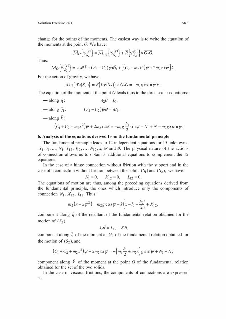
Solution Exercise 24.1 587
change for the points of the moments. The easiest way is to write the equation of
the moments at the point O. We have:
( ) ( ) ( ) 22 2 22 .T T T
O GS S SR G O= + ×
Thus: ( ) ( ) ( )
2
22 1 2 2 1 2 2 22T
O SA i A C j C m x m xx kθ ψθ ψ ψ = + − + + +
.
For the action of gravity, we have:
( ) ( ) 2 2 2 2e e sinO S R S G O m gx kψ= × = −
.
The equation of the moment at the point O leads thus to the three scalar equations:
along 1i
: 2 1,A Lθ =
along 1j
: ( )2 2 1,A C Mψθ− =
along k
:
( )2 11 2 2 2 1 1 22 sin sin .
2
hC C m x m x x m g N N m gxψ ψ ψ ψ+ + + = − + + −
6. Analysis of the equations derived from the fundamental principle
The fundamental principle leads to 12 independent equations for 15 unknowns:
1 1 1 12 12 12, , ... , ; , , ... , ; , and .X Y N X Y N x ψ θ The physical nature of the actions
of connection allows us to obtain 3 additional equations to complement the 12
equations.
In the case of a hinge connection without friction with the support and in the
case of a connection without friction between the solids 1( )S ans 2( ),S we have:
1 12 120, 0, 0.N X L= = =
The equations of motion are thus, among the preceding equations derived from
the fundamental principle, the ones which introduce only the components of
connection 1 12 12, , .N X L Thus:
( ) ( )2 22 2 0 12cos ,
2
hm x x m g k x l Xψ ψ− = − − − +
component along 1i
of the resultant of the fundamental relation obtained for the
motion of 2( ),S
2 12 ,A L Kθ θ= −
component along 1i
of the moment at 2G of the fundamental relation obtained for
the motion of 2( ),S and
( ) ( )2 11 2 2 2 1 2 12 sin ,
2
hC C m x m x x m m x g N Nψ ψ ψ+ + + = − + + +
component along k
of the moment at the point O of the fundamental relation
obtained for the set of the two solids.
In the case of viscous frictions, the components of connections are expressed
as:

588 Chapter 24 Other Examples of Motions of Rigid Bodies
12 1 1 12 2, , ,t r rX c x N c L cψ θ= − = − = −
where 1 2, and t r rc c c are the coefficients of viscous friction.
The three preceding equations of motion will allow us to obtain , and x θ ψas functions of time. Next, the components of the connections will be derived from the other equations.
24.2 Motion of a radar antenna (Figure 24.8)
1. Parameters of situation
1.1. Motion of the support (S1) with respect to the frame (T)
We associate the coordinate systems ( )Oxyz and ( )1 1Ox y z (Figure Exercise
24.2), respectively attached to the frame ( )T and to the support ( )1S . The upward
vertical axis Oz
coincides with the axis of rotation ( )1∆ .
We have one parameter of rotation ψ about the axis Oz
. The basis change is:
1
1
cos sin ,
sin cos ,
.
i i j
j i j
k
ψ ψ
ψ ψ
= +
= − +
1.2. Motion of the reflector (S2) with respect to the support (S1)
We associate (Figure Exercise 24.2) the systems ( )2 1 1G x y z and ( )2 1 2 2G x y z
respectively to the support ( )1S and to the reflector ( )2 .S The plane ( )2 1 2G x y is
contained in the plane of symmetry of the reflector.
We have one parameter of rotation θ about the axis 12 .G x
The basis change is:
1
2 1
2 1
,
cos sin ,
sin cos .
i
j j k
k j k
θ θ
θ θ
= + = − +
2. Kinematic study
2.1. Motion of the support (S1) with respect to the frame (T)
The kinematic torsor ( ) 1
TS relative to the motion of the support 1( )S with
respect to the frame ( )T has for elements of reduction at the mass centre 1G ,
located on the axis ( )1∆ of rotation:
( ) ( )
( ) ( )
1 1
1 11 1
, instantaneous rotation ivector,
( , ) 0, velocity vector of the point .
T TS S
T TG S
R k
G t G
ω ψ = =
= =
The acceleration vector of the mass centre is null: ( )
1( , ) 0.Ta G t =
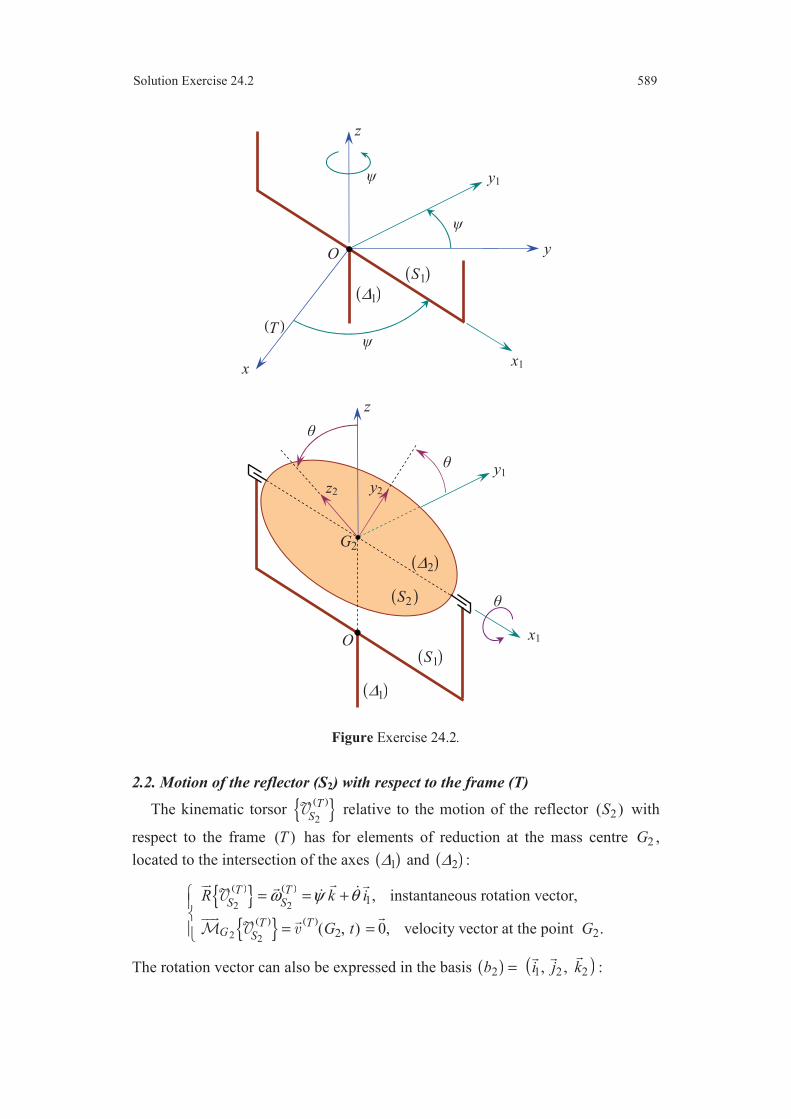
Solution Exercise 24.2 589
x
y
x1
y1
z
( )T
( )1∆
O
( )1S
x1
y1
z
( )1∆
O ( )1S
( )2S
( )2∆
2G
y2z2
Figure Exercise 24.2.
2.2. Motion of the reflector (S2) with respect to the frame (T)
The kinematic torsor ( ) 2
TS relative to the motion of the reflector 2( )S with
respect to the frame ( )T has for elements of reduction at the mass centre 2G ,
located to the intersection of the axes ( )1∆ and ( )2∆ :
( ) ( )
( ) ( )
2 2
2 2
1
2 2
, instantaneous rotation vector,
( , ) 0, velocity vector at the point .
T TS S
T TG S
R k i
G t G
ω ψ θ = = +
= =
The rotation vector can also be expressed in the basis ( )2b = ( )1 2 2, , i j k
:

590 Chapter 24 Other Examples of Motions of Rigid Bodies
( )
21 2 2sin cos .T
Si j kω θ ψ θ ψ θ= + +
The acceleration vector of the mass centre is null: ( )
2( , ) 0.Ta G t =
3. Kinetic study
3.1. Motion of the support (S1) with respect to the frame (T)
3.1.1. Kinetic torsor
The kinetic torsor ( ) 1
TS relative to the motion of the support (S1) with respect
to the frame has for elements of reduction at the mass centre:
( ) ( )
( ) ( ) ( )
1
1 11 1
1 1
1
( , ) 0,
,
T TS
T TG GS S
R m G t
S ω
= =
=
where 1m is the mass of the support 1( ).S
The operator of inertia at 1G is represented in the basis ( ) ( )1 1 1, , b i j k=
by the
matrix:
( ) ( )1
1
1 1 1
1 1 1 1
1 1 1
.b
G
A F E
S F B D
E D C
− − = − − − −
I
Hence:
( ) 1 1
1 1 1 1 1T
G SE i D j C kψ ψ ψ= − − +
.
3.1.2. Kinetic energy
The kinetic energy is given by:
( ) ( ) ( ) 1 1
c 11
( )2
T T TS S
E S = ⋅ .
Thus:
( ) 2c 1 1
1( )
2TE S Cψ= .
3.1.3. Dynamic torsor
The dynamic torsor ( ) 1
TS relative to the motion of the support (S1) with
respect to the frame has for elements of reduction at the point G1:
( ) ( )
( ) ( ) ( ) ( ) ( ) ( )
1
1 1 11 1 1 1
1 1
1 1
( , ) 0,
.
T TS
T T T TG G GS S S S
R m a G t
S Sω ω ω
= =
= + ×
The calculation of the moment leads to:
( ) ( ) ( )
1 1
2 21 1 1 1 1 1 1
TG S
D E i E D j C kψ ψ ψ ψ ψ= − − + +
.

Solution Exercise 24.2 591
3.2. Motion of the reflector (S2) with respect to the frame (T)
3.2.1. Kinetic torsor
The kinetic torsor ( ) 2
TS relative to the motion of the reflector (S2) with
respect to the frame has for elements of reduction at the mass centre 2G :
( ) ( )
( ) ( ) ( )
2
2 22 2
2 2
2
( , ) 0,
,
T TS
T TG GS S
R m G t
S ω
= =
=
where 2m is the mass of the reflector.
The reflector has a symmetry of cylindrical type. It follows that the operator of
inertia at 2G is represented in the basis ( ) ( )2 1 2 2, , b i j k=
by the matrix:
( ) ( )2
2
2
2 2
2
0 0
0 0 .
0 0
b
G
A
S A
C
=
I
The rotation vector ( )
2
TS
ω
was expressed previously in the basis ( )2b . It follows
that:
( ) 2 2
2 1 2 2 2 2sin cosTG S
A i A j C kθ ψ θ ψ θ= + +
.
3.2.2. Kinetic energy
The kinetic energy is expressed as:
( ) ( ) ( ) 2 2
c 21
( )2
T T TS S
E S = ⋅ .
Thus:
( ) ( )2 2 2 2c 2 2 2 2
1 1( ) sin cos
2 2TE S A A Cθ θ θ ψ= + + .
3.2.3. Dynamic torsor
The dynamic torsor ( ) 2
TS relative to the motion of the reflector (S2) with
respect to the frame ( )T has for elements of reduction at the mass centre 2G :
( ) ( )
( ) ( ) ( ) ( ) ( ) ( )
2
2 2 22 2 2 2
2 2
2 2
( , ) 0,
.
T TS
T T T TG G GS S S S
R m a G t
S Sω ω ω
= =
= + ×
The rotation vector ( )
2
TS
ω is obtained by deriving the expression of the rotation
vector ( )
2
TS
ω
in the basis ( )2b . Thus:
( ) ( ) ( )
21 2 2sin cos cos sin .T
Si j kω θ ψ θ ψθ θ ψ θ ψθ θ= + + + −
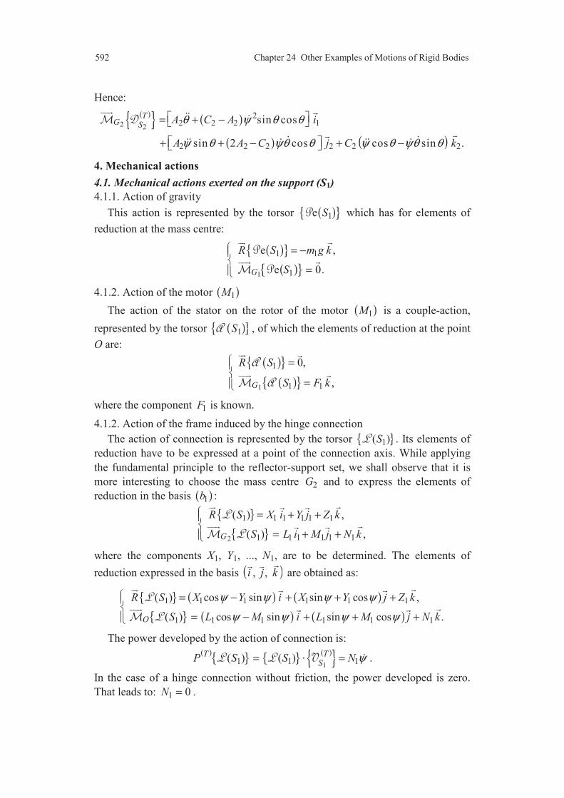
592 Chapter 24 Other Examples of Motions of Rigid Bodies
Hence:
( ) ( )
( ) ( )
2 2
22 2 2 1
2 2 2 2 2 2
sin cos
sin 2 cos cos sin .
TG S
A C A i
A A C j C k
θ ψ θ θ
ψ θ ψθ θ ψ θ ψθ θ
= + −
+ + − + −
4. Mechanical actions
4.1. Mechanical actions exerted on the support (S1)
4.1.1. Action of gravity
This action is represented by the torsor ( ) 1e S which has for elements of
reduction at the mass centre:
( )
( )
1
1 1
1
e ,
e 0.G
R S m g k
S
= −
=
4.1.2. Action of the motor ( )1M
The action of the stator on the rotor of the motor ( )1M is a couple-action,
represented by the torsor ( ) 1S , of which the elements of reduction at the point
O are:
( )
( ) 1
1
1 1
0,
,G
R S
S F k
=
=
where the component 1F is known.
4.1.2. Action of the frame induced by the hinge connection
The action of connection is represented by the torsor 1( )S . Its elements of
reduction have to be expressed at a point of the connection axis. While applying
the fundamental principle to the reflector-support set, we shall observe that it is
more interesting to choose the mass centre 2G and to express the elements of
reduction in the basis ( )1b :
2
1 1 1 1 1 1
1 1 1 1 1 1
( ) ,
( ) ,G
R S X i Y j Z k
S L i M j N k
= + +
= + +
where the components X1, Y1, ..., N1, are to be determined. The elements of
reduction expressed in the basis ( ), , i j k
are obtained as:
( ) ( )
( ) ( )
1 1 1 1 1 1
1 1 1 1 1 1
( ) cos sin sin cos ,
( ) cos sin sin cos .O
R S X Y i X Y j Z k
S L M i L M j N k
ψ ψ ψ ψ
ψ ψ ψ ψ
= − + + +
= − + + +
The power developed by the action of connection is:
( ) ( ) 1
1 1 1( ) ( )T TS
P S S N ψ= =⋅ .
In the case of a hinge connection without friction, the power developed is zero.
That leads to: 1 0N = .
Solution Exercise 24.2 593
4.1.4. Action of the motor ( )2M
The action of the rotor on the stator of the motor ( )2M is represented by the
torsor ( ) 2 1 .S This action is opposed to the action exerted by the stator on the
rotor, then to the action exerted by the motor on the reflector ( )2 .S This action is
represented by the torsor ( ) 1 2 .S We have:
( ) ( ) 2 1 1 2 .S S= −
The torsor ( ) 1 2S will be expressed afterwards.
4.1.5. Action of the reflector induced by the hinge connection between ( )1S and
( )2S
This action is represented by the torsor ( ) 2 1 .S It is opposed to the action of
connection exerted by the support ( )1S on the reflector ( )2S and represented by
the torsor ( ) 1 2S :
( ) ( ) 2 1 1 2 .S S= −
We shall express the torsor ( ) 1 2S in the following paragraph.
4.2. Mechanical actions exerted on the reflector (S2) 4.2.1. Action of gravity
This action is represented by the torsor ( ) 2e S which has for elements of
reduction at the mass centre 2G :
( )
( )
2
2 2
2
e ,
e 0.G
R S m g k
S
= −
=
4.2.2. Action of the motor ( )2M
The action of the stator on the rotor of the motor ( )2M is a couple-action,
represented by the torsor ( ) 1 2S , of which the elements of reduction at the
point G2 are:
( )
( ) 2
1 2
1 2 2 1
0,
,G
R S
S F i
=
=
where the component 2F is known.
4.2.3. Action of the support ( )1S induced by the hinge connection with the reflector
This action is represented by the torsor 1 2( )S of elements of reduction at the
point 2G , which we express in the basis ( )1b :
2
1 2 12 1 12 1 12
1 2 12 1 12 1 12
( ) ,
( ) .G
R S X i Y j Z k
S L i M j N k
= + +
= + +
The components X12, Y12, ..., N12, are to be determined. In the case of a
connection without friction, we have: 12 0.L =
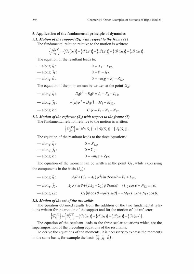
594 Chapter 24 Other Examples of Motions of Rigid Bodies
5. Application of the fundamental principle of dynamics
5.1. Motion of the support (S1) with respect to the frame (T)
The fundamental relation relative to the motion is written:
( ) ( ) ( ) 1
1 1 1 2 1 2 1e ( ) ( ) ( ) .TS
S S S S S= + + + +
The equation of the resultant leads to:
along 1i
: 1 120 ,X X= −
along 1j
: 1 120 ,Y Y= −
along k
: 1 1 120 .m g Z Z= − + −
The equation of the moment can be written at the point 2G :
along 1i
: 21 1 1 2 12,D E L F Lψ ψ− = − −
along 1j
: ( )21 1 1 12,E D M Mψ ψ− + = −
along k
: 1 1 1 12.C F N Nψ = + −
5.2. Motion of the reflector (S2) with respect to the frame (T)
The fundamental relation relative to the motion is written:
( ) ( ) 2
2 1 2 1 2e ( ) ( ) .TS
S S S= + +
The equation of the resultant leads to the three equations:
along 1i
: 120 ,X=
along 1j
: 120 ,Y=
along k
: 2 120 .m g Z= − +
The equation of the moment can be written at the point 2G , while expressing
the components in the basis ( )2b :
along 1i
: ( ) 22 2 2 2 12sin cos ,A C A F Lθ ψ θ θ+ − = +
along 2j
: ( )2 2 2 12 12sin 2 cos cos sin ,A A C M Nψ θ ψθ θ θ θ+ − = +
along 2k
: ( )2 12 12cos sin sin cos .C M Nψ θ ψθ θ θ θ− = − +
5.3. Motion of the set of the two solids
The equation obtained results from the addition of the two fundamental rela-
tions written for the motion of the support and for the motion of the reflector: ( ) ( ) ( ) ( )
1 21 1 1 2e ( ) ( ) eT T
S SS S S S+ = + + + .
The equation of the resultant leads to the three scalar equations which are the
superimposition of the preceding equations of the resultants.
To derive the equations of the moments, it is necessary to express the moments
in the same basis, for example the basis ( )1 1, , i j k
.
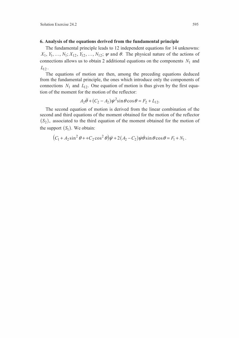
Solution Exercise 24.2 595
6. Analysis of the equations derived from the fundamental principle
The fundamental principle leads to 12 independent equations for 14 unknowns:
1 1 1 12 12 12, , ... , ; , , ... , ; and .X Y N X Y N ψ θ The physical nature of the actions of
connections allows us to obtain 2 additional equations on the components 1N and
12L .
The equations of motion are then, among the preceding equations deduced
from the fundamental principle, the ones which introduce only the components of
connections 1N and 12.L One equation of motion is thus given by the first equa-
tion of the moment for the motion of the reflector:
( ) 22 2 2 2 12sin cos .A C A F Lθ ψ θ θ+ − = +
The second equation of motion is derived from the linear combination of the
second and third equations of the moment obtained for the motion of the reflector
( )2 ,S associated to the third equation of the moment obtained for the motion of
the support ( )1 .S We obtain:
( ) ( )2 21 2 2 2 2 1 1sin cos 2 sin cosC A C A C F Nθ θ ψ ψθ θ θ+ + + + − = + .

Chapter 25
The Lagrange Equations
25.1 Lagrange equations relative to the motion of the set of the two solids studied in Exercise 24.1
In fact, the elements necessary to establish the Lagrange equations have been
expressed in the correct version of Exercise 24.1.
The Lagrange equations for the set ( )D constituted of the two solids ( )1S and
( )2S are written from (25.39):
( )( ) ( )( ) ( ) ( ) ( ) ( ) ( ) ( ) ( ) ( ) ( ) ( ) ( ) ( ) ( ) ( ) ( ) ( )
c c 1 1 2 1
1 1 2 2 1 2
de
d
e .
i i i
i i i i i
T T T T Tq q q
i iT T T T T
q q q q q
E D E D P S P S P St q q
P S P S P S P S P S
∂ ∂− = + +
∂ ∂
+ + + + +
This equation introduces the power coefficients in the reference ( )T of all the
actions exerted on the two solids ( )1S and ( )2 .S The three equations which are
deduced from this equation are relative to the three parameters of situation:
, , .iq x ψ θ=The kinetic energy of the set is:
( ) ( ) ( ) ( ) ( ) ( )c c 1 c 2T T TE D E S E S= + ,
where the kinetic energies relative to the motions of the solids ( )1S and ( )2S have
been expressed in the correct version of Exercise 24.1. Hence:
( ) ( ) ( ) 2 2 2 2 2c 1 2 2 2 2
1 1 1 1.
2 2 2 2TE D C C m x m x Aψ ψ θ== + + + +
The power coefficients are deduced from the expressions of the powers deve-
loped by the different actions exerted. Some ones were expressed in the correct
version of Exercise 24.4. It remains to evaluate:
the power developed by the action of connection of ( )2S on ( )1S :
( ) ( ) ( ) 1 1
2 1 2 1 1 2( ) ( ) ( )T T TS S
P S S S= = −⋅ ⋅ .
( ) ( )2 1 12 12( )TP S N xY ψ= − + .
the power developed by the action of the spring on ( )1S :
( ) ( ) ( ) 1 1
1 1 2( ) ( ) ( )T T TS S
P S S S= = − ⋅⋅ .
( ) 1( ) 0TP S = .
the power developed by the action of the spring on ( )2S :
( ) ( ) ( ) ( )
2 2 22 2 1 2 2 2( ) ( ) ( ) ( )T T T T
S S SP S S S S= = +⋅ ⋅ ⋅ .
( ) ( )22 0( ) .
2T h
P S k x l x Kθθ= − − − −
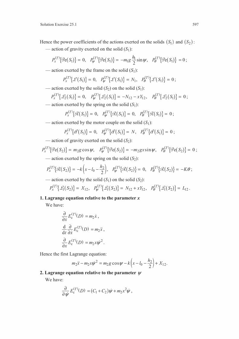
Solution Exercise 25.1 597
Hence the power coefficients of the actions exerted on the solids ( )1S and ( )2S :
— action of gravity exerted on the solid (S1):
( ) ( ) ( ) ( ) ( ) ( ) 11 1 1 1e 0, e sin , e 0
2T T T
xh
P S P S m g P Sψ θψ= = − = ;
— action exerted by the frame on the solid (S1):
( ) ( ) ( ) ( ) ( ) ( ) 1 1 1 10, , 0T T TxP S P S N P Sψ θ= = = ;
— action exerted by the solid (S2) on the solid (S1):
( ) ( ) ( ) ( ) ( ) ( ) 2 1 2 1 12 12 2 10, , 0T T TxP S P S N xY P Sψ θ= = − − = ;
— action exerted by the spring on the solid (S1):
( ) ( ) ( ) ( ) ( ) ( ) 1 1 10, 0, 0T T TxP S P S P Sψ θ= = = ;
— action exerted by the motor couple on the solid (S1):
( ) ( ) ( ) ( ) ( ) ( ) 1 1 10, , 0T T TxP S P S N P Sψ θ= = = ;
— action of gravity exerted on the solid (S2):
( ) ( ) ( ) ( ) ( ) ( ) 2 2 2 2 2e cos , e sin , e 0T T TxP S m g P S m gx P Sψ θψ ψ= = − = ;
— action exerted by the spring on the solid (S2):
( ) ( ) ( ) ( ) ( ) ( ) ( ) 22 0 2 2, 0,
2T T T
xh
P S k x l P S P S Kψ θ θ= − − − = = − ;
— action exerted by the solid (S1) on the solid (S2):
( ) ( ) ( ) ( ) ( ) ( ) 1 2 12 1 2 12 12 1 2 12, , T T TxP S X P S N xY P S Lψ θ= = + = .
1. Lagrange equation relative to the parameter x
We have:
( )( )c 2TE D m x
x
∂=
∂
,
( )( )c 2
d
dTE D m x
t x
∂=
∂
,
( )( ) 2c 2TE D m x
xψ∂
=∂
.
Hence the first Lagrange equation:
( )2 22 2 2 0 12cos .
2
hm x m x m g k x l Xψ ψ− = − − − +
2. Lagrange equation relative to the parameter ψ
We have:
( )( ) ( ) 2c 1 2 2TE D C C m xψ ψ
ψ∂
= + +∂
,
598 Chapter 25 The Lagrange Equations
( )( ) ( )2c 1 2 2 2
d2
dTE D C C m x m xx
tψ ψ
ψ∂
= + + +∂
,
( )( )c 0TE D
ψ∂
=∂
.
Hence the second Lagrange equation:
( )2 11 2 2 2 1 1 22 sin sin
2
hC C m x m xx m g N N m gxψ ψ ψ ψ+ + + = − + + − .
3. Lagrange equation relative to the parameter
We have:
( )( )c 2TE D A θ
θ∂
=∂
,
( )( )c 2
d
dTE D A
t xθ∂
=∂
,
( )( )c 0TE D
x
∂=
∂.
Hence the third Lagrange equation:
2 12A K Lθ θ= − + .
We find again the third equations of motion derived from the fundamental prin-
ciple of dynamics (correct version of Exercise 24.1).
25.2 Lagrange equations relative to the motion of the radar antenna
The Lagrange equations relative to the motion of the set ( )D constituted of the
support ( )1S of the antenna and of its reflector ( )2S are written:
( )( ) ( )( ) ( ) ( ) ( ) ( ) ( ) ( ) ( ) ( ) ( ) ( ) ( ) ( ) ( ) ( ) ( ) ( )
c c 1 1 1
2 1 2 1 2 1 2 1 2
de
d
e ,
i i i
i i i i i
T T T T Tq q q
i iT T T T T
q q q q q
E D E D P S P S P St q q
P S P S P S P S P S
∂ ∂− = + +
∂ ∂
+ + + + +
, .iq ψ θ=
The kinetic energy of the set is the sum of the kinetic energies expressed in the
correct version of Exercise 24.2. Thus:
( ) ( )2 2 2 2c 1 2 2 2
1 1( ) sin cos
2 2TE D C A C Aθ θ ψ θ= + + + .
So as to obtain the power coefficients, we express the powers developed by the
actions exerted on the two solids:
( ) ( ) ( ) ( ) ( ) ( ) 1 1 1 1 1e 0, , ,T T TP S P S F P S Nψ ψ= = =
( ) ( ) ( ) ( ) 2 1 12 2 1 12, ,T TP S F P S Nψ ψ= − = −
( ) ( ) ( ) ( ) ( ) ( ) 2 1 2 2 1 2 12 12e 0, , .T T TP S P S F P S L Nθ θ ψ= = = +
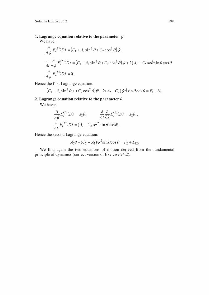
Solution Exercise 25.2 599
1. Lagrange equation relative to the parameter ψWe have:
( )( ) ( )2 2c 1 2 2sin cosTE D C A Cθ θ ψ
ψ∂
= + +∂
,
( )( ) ( ) ( )2 2c 1 2 2 2 2
dsin cos 2 sin cos
dTE D C A C A C
tθ θ ψ ψθ θ θ
ψ∂
= + + + −∂
,
( )( )c 0TE D
ψ∂
=∂
.
Hence the first Lagrange equation:
( ) ( )2 21 2 2 2 2 1 1sin cos 2 sin cosC A C A C F Nθ θ ψ ψθ θ θ+ + + + − = +
2. Lagrange equation relative to the parameter
We have:
( )( ) ( )( )c 2 c 2
d, ,
dT TE D A E D A
t xθ θ
θ∂ ∂
= =∂∂
,
( )( ) ( ) 2c 2 2 sin cosTE D A C
xψ θ θ∂
= −∂
.
Hence the second Lagrange equation:
( ) 22 2 2 2 12sin cos .A C A F Lθ ψ θ θ+ − = +
We find again the two equations of motion derived from the fundamental
principle of dynamics (correct version of Exercise 24.2).


Printed in France by Jean-Marie Berthelot
Les Clousures, Chemin des Horts
05290 Vallouise
France


The book "Mechanics of Rigid Bodies" develops a unified approach to the
problems of the Mechanics of Solids.
The development is based on a generalized use of the concept of “torseur” (in
French). We think that this concept is not used in the English textbooks. We will
call this concept as “torsor”.
After a first part where the necessary elements of mathematics are recalled, the
book is structured through four parts of increasing difficulties in such a way to
have a good assimilation of the concepts.
A sixth part analyses the numerical methods used to solve the motion
equations. Comments reported at the end of each chapter summarize the
fundamental notions which must which must be acquired.
Examples and simple exercises are associated to each chapter with the object to
familiarize the reader with the fundamental tools needed to solve the problems of
Mechanics of Solids.
A last part develops the solutions of the exercises which are proposed all along
the book.
Jean-Marie Berthelot is an Honorary Professor, Maine University, Le Mans France. He took part at the installation of the Institute for Advanced Materials and Mechanics (ISMANS), Le Mans, France. His current research is on the mechanical behaviour of composite materials and structures. He has published extensively in the area of composite materials and is the author of different textbooks, in particular of the textbook entitled Composite
Materials, Mechanical Behavior and Structural Analysis published by Springer, New York, in 1999.