J Electr Eng Technol.2016; 11(?): 0-000 http://dx.doi.org/10.5370/JEET.2016.11.3.0

0Copyright ⓒ The Korean Institute of Electrical Engineers

This is an Open-Access article distributed under the terms of the Creative Commons Attribution Non-Commercial License (http://creativecommons.org/ licenses/by-nc/3.0/) which permits unrestricted non-commercial use, distribution, and reproduction in any medium, provided the original work is properly cited.

Hourly Average Wind Speed Simulation and Forecast Based on ARMA Model in Jeju Island, Korea

Duy-Phuong N. Do*, Yeonchan Lee** and Jaeseok Choi†

Abstract – This paper presents an application of time series analysis in hourly wind speed simulation and forecast in Jeju Island, Korea. Autoregressive – moving average (ARMA) model, which is well in description of random data characteristics, is used to analyze historical wind speed data (from year of 2010 to 2012). The ARMA model requires stationary variables of data is satisfied by power law transformation and standardization. In this study, the autocorrelation analysis, Bayesian information criterion and general least squares algorithm is implemented to identify and estimate parameters of wind speed model. The ARMA (2,1) models, fitted to the wind speed data, simulate reference year and forecast hourly wind speed in Jeju Island.

Keywords: Autoregressive moving average processes, Autoregressive processes, Autocorrelation function, Time series model, Wind energy, Wind speed forecast, Wind speed simulation

1. Introduction

Nowadays, the penetration of wind power continues to increase in power system, especially in Korea. Wind is considered as an energy credit but it is also fluctuation. It needs to access economic and technological factors. The study of wind power forecast, comprehensive reliability and cost evaluation of the system is the answer. An essential step in the study is to model the wind speed of specific site. The wind speed model is used to reproduce accurately actual wind speed. The analysis of historical wind speed data is to determine the necessary parameters for the model.

Data of hourly average wind speed (HAWS) in a specific location is time series, which has the following basic characteristics. Firstly, it is numeric statistics whose characteristics are illustrated by specific parameters such as probability distribution, mean value, standard deviation. Secondly, the values of time series have a correlation that means the relation of the present time value to past time values. This correlation is reflected by auto-correlation functions (ACF) and partial auto-correlation functions (PACF). Ones of the favorite methods in modeling correlation characteristics of time series is Box-Jenkins methodology or Autoregressive moving average (ARMA) process. The ARMA models can use 3 years of historical HAWS data in Jeju Island and result in accurate short-term forecast of HAWS [11]. There are three classes of ARMA processes. Autoregressive AR(p) process has characteristics that the present time data value is defined by p previous time values and white noise. Moving average

MA(q) process has the present time data value which is defined by a weighted moving average of the noise pulse. And autoregressive moving average ARMA(p, q) process is mixed of the autoregressive and moving average characteristics [2].

Many previous studies had fitted ARMA process to wind speed data. These papers proposed the general approach for modeling wind speed [1] and case study of wind speed statistical models in specific site or multiple sites [3, 4, 6, 10-12]. The wind speed data were almost transformed from Weibull distribution to normal distribution by Dubey method which the shape parameters of data is transformed to 3.6 and the power m for the transformation was specified by measure of distribution symmetry [1], Skewness method [3, 4, 6, 10] or by Box-Cox method which the power λ for the transformation is specified by minimizing the Skewness of the data [8]. However, the transformed data was not checked the strongly stationary [1, 10] or instead of checking the strongly stationary of transformed data, normal distribution is only considered by comparing with corresponding normal probability density [3, 4, 8] or testing non-stationary of transformed data by Duckey-fuller test [9]. These papers assumed that transformed data fitted to a pth order autoregressive process AR(p) [1] or the transformed data fitted to a pth order autoregressive process AR(p) by autocorrelation, partial autocorrelation analysis in identification process but there was no using Bayesian information criterion (BIC) to select an accurate class of ARMA(p,q) [3] or ACF, PACF and BIC were analyzed but the AR(p) was selected too soon after ACF and PACF analysis [8], instead of analyzing ACF, PACF and BIC together or using only AIC [9, 10].

From above analyses, this paper presents ARMA model application to wind speed simulation and forecast in

† Corresponding Author: Dept. of Electrical Engineering, Gyeongsang National University, Korea. (jschoi@gnu.ac.kr)

* Dept. of Electrical Engineering, Gyeongsang National University,Korea. ({dndphuong, kkng1914}@gnu.ac.kr)

Received: June 25, 2015; Accepted: July 28, 2016

ISSN(Print) 1975-0102ISSN(Online) 2093-7423

Proofreading

spJearwlineofandibyacHm

secavawsesoAdastapmmwreobth

F

pecific site, Jeeju Island arere transformed

which the powkelihood funcew way is prof transformednalysis and istribution chy analyzing Accurate class

HAWS data frmeteorological

2. St An importa

eries model isan easily be dariance. ARM

which are normeasonal compome phases in

ARMA modelata which hatationary, andpproximately

models are estmodels are chewind speeds isequires the stbservation V he daily variat

Janu

Ju

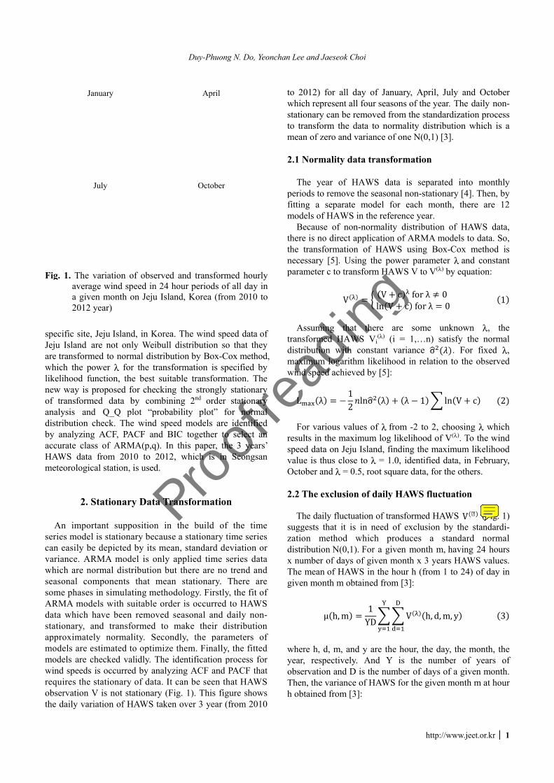
Fig. 1. The vaaveragea given 2012 ye

eju Island, in e not only Wd to normal d

wer λ for the ction, the besoposed for chd data by coQ_Q plot “

heck. The winACF, PACF aof ARMA(p,

from 2010 tol station, is use

ationary Da

ant suppositios stationary bdepicted by itMA model is mal distributiponents that n simulating ms with suitab

ave been remd transforme

y normality. timated to optecked validly.s occurred by ationary of dais not stationtion of HAWS

uary

uly

ariation of obe wind speed i

month on Jejear)

Duy

Korea. The wWeibull distribudistribution by

transformatiost suitable trahecking the stombining 2nd

“probability pnd speed modand BIC toge,q). In this pa 2012, whiched.

ata Transfor

on in the buecause a statits mean, stanonly applied

ion but there mean statio

methodology.le order is oc

moved seasonaed to make tSecondly, thtimize them. . The identificanalyzing ACata. It can be ary (Fig. 1). TS taken over 3

O

served and trin 24 hour perju Island, Kor

y-Phuong N. Do

wind speed daution so that

y Box-Cox meon is specifiedansformation. trongly statio

d order statioplot” for nodels are identether to selecaper, the 3 yeh is in Seon

rmation

uild of the ionary time se

ndard deviatiod time series

are no trend onary. There . Firstly, the fccurred to HAal and daily ntheir distribu

he parameterFinally, the fcation processCF and PACF seen that HAThis figure sh3 year (from 2

April

October

ransformed horiods of all darea (from 201

o, Yeonchan Le

ata of they

ethod, d by The

onary onary rmal ified

ct an ears’ gsan

time eries on or data and are

fit of AWS non-ution s of

fitted s for that

AWS hows 2010

to 2whistatito tmea

2.1

Tperifittimod

Btherthenecpara

Atrandistmaxwin

LF

resuspeevaluOct

2.2

Tsuggzatidistx nuThegive

wheyearobsTheh ob

ourly ay in 10 to

e and Jaeseok C

2012) for all ich represent aionary can be transform the an of zero and

Normality d

The year of iods to removng a separatdels of HAWS

Because of nore is no direct

transformatioessary [5]. Uameter c to tra

VAssuming thansformed HAWtribution withximum logaritnd speed achie

L λ 12For various vaults in the maxed data on Jejue is thus clostober and λ =

The exclusio

The daily fluctugests that it iion methodtribution N(0,1umber of dayse mean of HAWen month m ob

μ h,mere h, d, m, anr, respectivelervation and D

en, the variancbtained from [

Choi

day of Januaall four seasonremoved fromdata to norm

d variance of o

data transfor

HAWS data e the seasonalte model for S in the refereon-normality application o

on of HAWSUsing the powansform HAWV cln Vat there areWS Vi

(λ) (i =h constant vathm likelihoo

eved by [5]: 12 lnσ λalues of λ fromximum log likju Island, findse to λ = 1.0,0.5, root squa

on of daily H

uation of transis in need of

which prod1). For a gives of given mo

AWS in the hobtained from

1YDnd y are the hly. And Y iD is the numbce of HAWS f[3]:

http://w

ary, April, Juns of the year. m the standard

mality distribuone N(0,1) [3]

rmation

is separatedl non-stationa

each monthence year. distribution o

of ARMA modS using Box-wer parameter WS V to V(λ) byc forλ 0c forλ 0e some unk= 1,…n) satiariance σd in relation

λ 1 lnm -2 to 2, chkelihood of Vding the maxim, identified daare data, for th

HAWS fluctu

sformed HAWf exclusion byduces a sta

en month m, honth x 3 yearsur h (from 1 t[3]:

V h, d,m,hour, the day,is the numbeber of days offor the given m

www.jeet.or.kr │

uly and OctobThe daily no

dization proceution which is

.

d into monthary [4]. Then, bh, there are

of HAWS datdels to data. SCox method λ and consta

y equation:

known λ, tisfy the norm. For fixed to the observ

n V c oosing λ whi

V(λ). To the winmum likelihooata, in Februarhe others.

ation

WS V (Fig.y the standardandard normhaving 24 hous HAWS valueto 24) of day

, y , the month, ter of yearsf a given montmonth m at ho

1

ber on-ess s a

hly by 12

ta, So,

is ant

1

the mal

λ, ed

2

ch nd od ry,

1) di-

mal urs es. in

3

the of th.

our

Proofreading

2

an

2

stmgiby

ex

ofFw±deoravstwdi

F

│ J Electr Eng

σ h,m Y From these

nd transforme h, d,m

.3 Results of As above m

tationary datamodel [2]. Th

iven month y 2 steps. Firstly, check

xpression:

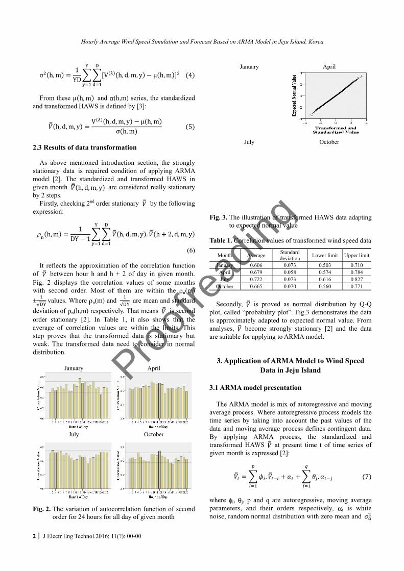
ρ h,m D It reflects th

f betweenig. 2 display

with second o

√ values. Weviation of ρn

rder stationarverage of cortep proves th

weak. The tranistribution.

Janu

Ju

Fig. 2. The varorder fo

Hourly Aver

Technol.2016;

1YD Vµ h,m and

ed HAWS is d

m, y V h,f data transfo

mentioned intra is required

he standardizeh, d,m, y a

king 2nd order

1DY 1he approximatn hour h and ys the correlaorder. Most o

Where ρn(m) a

n(h,m) respectry [2]. In Tarrelation valuhat the transfnsformed dat

uary

uly

riation of autoor 24 hours for

rage Wind Spee

11(?): 00-00

h, d,m, yσ(h,m) series

defined by [3]:, d,m, y μσ h,mormation

roduction seccondition of

ed and transfare considered

r stationary

h, d,m, ytion of the coh + 2 of dayation values of them are and √ are mtively. That mable 1, it alsoues are withinformed data ta need to co

O

ocorrelation fur all day of giv

ed Simulation a

μ h,m , the standard h,m tion, the stroapplying AR

formed HAWd really statio

by the follow

. h 2, d,morrelation funcy in given mo

of some mowithin the ρ

mean and stanmeans is sec

o shows thatn the limits. is stationary

onsider in nor

April

October

function of secven month

nd Forecast Ba

4

dized

5

ongly RMA S in

onary

wing

m, y

(6)

ction onth. onths

n(m) ndard cond t the This

y but rmal

cond

Fig

Tab

M

Ja

O

Splotis aanalare

3

3.1

TavertimedataBy trangive

wheparanois

ased on ARMA M

Januar

July

. 3. The illustrto expecte

ble 1. Correlat

Month Ave

anuary 0.6April 0.6July 0.7

October 0.6

Secondly, it, called “probapproximatelylyses, becosuitable for ap

3. Applicatio

ARMA mod

The ARMA mrage process. e series by taa and moving

applying Ansformed HAWen month is ex

ere φi, θj, p aameters, andse, random no

Model in Jeju Is

ry

ration of transed normal valu

tion values of

erage Standdeviat

606 0.07679 0.05722 0.07665 0.07

s proved as bability plot”.

y adapted to eome strongly pplying to AR

on of ARMAData in Je

del presentat

model is mix oWhere autore

aking into accg average procARMA proceWS at presxpressed [2]:

.and q are autod their ordersormal distribu

Island, Korea

Ap

Octo

sformed HAWue

transformed w

dard tion Lower l

73 0.50358 0.57473 0.61670 0.560

normal distri. Fig.3 demonexpected norm

stationary [2RMA model.

A Model to Weju Island

ion

of autoregressegressive proccount the pascess defines cess, the stasent time t of

.oregressive, ms respectivelution with zer

pril

ober

WS data adaptin

wind speed da

limit Upper lim

3 0.7104 0.7846 0.8270 0.771

ibution by Q-nstrates the damal value. Fro2] and the da

Wind Speed

ive and movincess models tst values of tcontingent datandardized anf time series

moving averaly, αt is whiro mean and σ

ng

ata

mit

-Q ata om ata

ng the the ta. nd of

7

age ite σ

Proofreading

va

3

paorgies

wau

ofco

ofw

F

ariance.

.2 Wind spee Wind speed

artial autocorrder of modeiven month stimated by Yu

c m H

where H = 24 utocorrelation

Applying thi

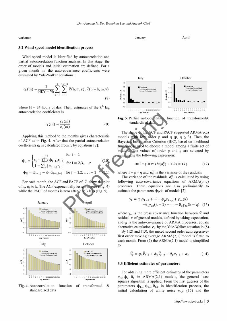
f ACF as in Foefficients φk

ϕ r1ϕ ϕ , For each mo

f rk, φk to k. Twhile the PACF

Jan

J

Fig. 4. Autocostandard

ed model ide

model is iderrelation functels and initial

m, the autoYule-Walker eq

1DY Ykhours of day

n coefficients i

is method to Fig. 4. After is calculated fr ∑ ϕ , r∑ ϕ , rϕ ϕ ,

onth, the ACF The ACF expoF of months is

nuary

July

rrelation fudized data

Duy

entification p

entified by aution analysis.

estimation a-covariance

quations:

h,m, yy. Then, estimis

the months githat the partifrom rk by equfori 1fori 2,3forj 1,2and PACF of

onentially lesss zero after 2 o

unction of

y-Phuong N. Do

process

utocorrelation In this stage

are defined. Fcoefficients w

y . h k,mates of the kth

ives characterial autocorrelauations [2]:

3,… , n, … , i 1f show theen to zero (Fior 3 lags (Fig.

April

October

transformed

o, Yeonchan Le

and , the

For a were

m, y (8)

h lag

9

ristic ation

10

11

plot g. 4) . 5).

&

Fig

TmodBayfuncmodmin

wheT

follprocestim

wheresiandalter

Bfirsteachto

3.3

Fϕ ,squparainit

e and Jaeseok C

Januar

July

. 5. Partial austandardiz

The shape of tdels with lowyesian Informaction, is useddels. The va

nimizing the fo

BIC =

ere T = p + q aThe variance oowing auto-cesses. Thesmate the param

γ ϕ γ

ere γza is the dual of gue

d γk is the autornative calcula

By (12) and (1t order movinh month. From

Efficient est

For obtaining mϕ , θ in Aares algorithmameters ϕ , ,ial calculatio

Choi

ry

utocorrelationzed data

the ACF and Pw order p anation Criterio

d to choose a alues of ordeollowing expr

= (HDY) ln(σand σ is the of the residua-covariance e equations meters ϕ , θ γ ⋯ ϕθ γ k 1cross covariassed models, do-covariance ation c by th3), the mixed

ng average ARm (7) the AR

timates of pa

more efficienARMA(2,1) m is applied. F, ϕ , , θ , in on of white

http://w

A

Oct

n function of

PACF suggestnd q (p, q ≤n (BIC), basemodel among

er p and q aression:

) + T ln(HDY

variance of thals σ is calcuequations ofare also p

of models [2]γ γ k⋯ θ γance function defined by takof ARMA pr

he Yule-Walked second orderRMA(2,1) m

RMA(2,1) mod

arameters

nt estimates ofmodels, the

From the firstidentificatio

e noise α ,www.jeet.or.kr │

April

tober

f transformed

ted ARMA(p,≤ 3). Then, ted on likelihoog a finite set are selected b

Y) (1

he residualsulated by usinf ARMA(p,reliminarily]. k k q (1between an

king expectatiorocesses, equar equation in (

r autoregressivodel is fitted del is simplifi

1f the paramete

general leat guesses of t

on process, th (15) and th

3

d&

,q) the od of by

2)

ng q) to

3)

nd on, als (8). ve-to ed

4

ers ast the he he

Proofreading

4

deobsere

wto

guli

adevthcaT

3

byrkmdipoKmdist

T

│ J Electr Eng

erivatives of btained. Theneries are set tecursions, as f

,,

where , is io φ, and xt is th

Expanding euesses of thenear regressio , By regressi

djustment is very iteration he new valualculated by

The results are

.4 Diagnostic Final stage i

y analyzing k(α). If the αt

means the rkistribution, thortmanteau la

K=24 autocormodels are a

istribution (2tatistic (Q-stat

Table 2. The pa

Months Jan 1Feb 1Mar 1Apr 1May 1Jun 1Jul 1

Aug 1Sep 1Oct 1Nov 1Dec 1

Hourly Aver

Technol.2016;

to paramn, the startingo zero and thfollows [2]

,, ,, , initial white nhe derivativesexpectation ofe parameters ϕon equation ob

, ., .ing , on added to the step. From t

ues of , , iteration procas in Tables 2

c checking o

is to check thautocorrelati

t’s series indick(α) will bhe fitted modack of fit testrrelations of approximately21 degrees otistic) is calcu

Q=HDY∑

arameter estim

φ1 φ2 .263 -0.309 .200 -0.263 .178 -0.254 .304 -0.360 .347 -0.388 .236 -0.281 .152 -0.204 .086 -0.132 .148 -0.200 .340 -0.376 .187 -0.255 .166 -0.229

rage Wind Spee

11(?): 00-00

meter of modeg values for αhen calculated

, , noise, ut is thes of αt to θ. f αt in a Tayloϕ , , ϕ , , θ ,btained:

, ,

guesses of the new guess

, cess until con2.

f fitted mode

he proposed mion function cates the natu

be uncorrelatdels are accet” to considerthe residualsy distributedof freedom). ulated by:

( )K

2k

k=1

r α∑

mates of ARM

θ1 0.701 00.597 00.555 00.626 00.653 00.620 00.550 00.437 00.514 00.729 00.582 00.599 0

ed Simulation a

els (16) and αt’s, xt’s, and

d with the forw

, e derivatives o

or series with , an approxim

, . , and ,the parameterses of parame

, and nvergence occ

el

models in Tabof the resid

ure of models ted and noreptable. Usingr whether the s of ARMA(d as Chi-sq

The Box-Pi

MA(2,1) mode

σ Q-stati0.447 20.50.405 28.30.410 16.170.359 18.340.306 19.20.335 30.20.320 38.220.221 33.20.284 26.90.393 24.740.408 30.30.418 36.34

nd Forecast Ba

(17) d ut’s ward

15 16 17

of αt

first mate

(18)

the rs in eters,

are curs.

ble 2 duals

that rmal g “a first

(2,1) quare ierce

(19)

Rsqu1% The

Tgensequhavvariserihouobta

whestangive

Fig

Fig

Aut

ocor

rela

tion

Aut

ocor

rela

tion

ls

stic3 5 7 4 9 3 2 5 1 4 6 4

ased on ARMA M

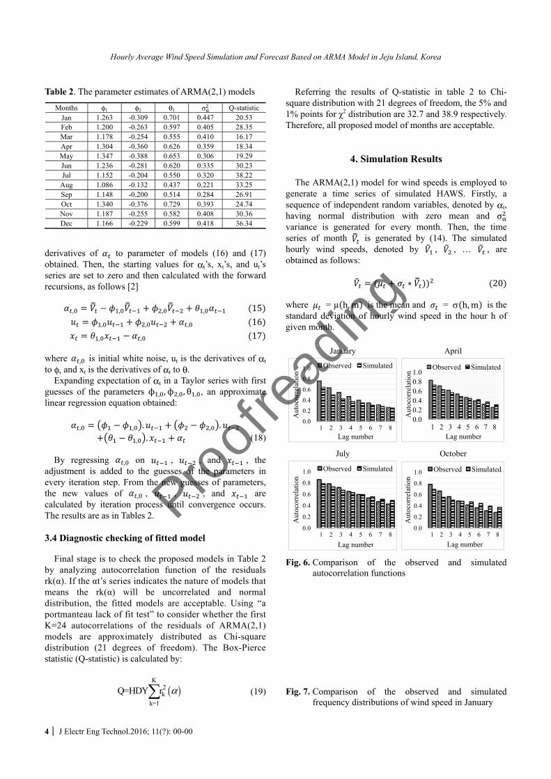
Referring the are distributiopoints for χ2 d

erefore, all pro

The ARMA(2,nerate a timeuence of inde

ving normal iance is genees of month

urly wind spained as follow

ere = µ h,ndard deviatioen month.

Janua

July

. 6. Comparisautocorrel

. 7. Comparisfrequency

0.00.20.40.60.81.0

1 2 3Lag

Observed

0.0

0.2

0.4

0.6

0.8

1.0

1 2 3Lag

Observed

Model in Jeju Is

results of Qon with 21 degdistribution aroposed model

4. Simulatio

,1) model for e series of sependent rand

distribution erated for ev

is generaeeds, denotews:

, m is the meon of hourly w

ary

y

on of the lation function

on of the y distributions

4 5 6 7 8g number

d Simulated

4 5 6 7 8g number

d Simulated

Island, Korea

Q-statistic in tgrees of freedre 32.7 and 38of months are

on Results

wind speeds imulated HAom variables,with zero

very month. Tated by (14). d by ,

∗ ean and =wind speed in

A

Oc

observed ns

observed of wind speed

0.00.20.40.60.81.0

1 2

Aut

ocor

rela

tion

L

Obser

0.0

0.2

0.4

0.6

0.8

1.0

1 2

Aut

ocor

rela

tion

L

Obse

table 2 to Chom, the 5% an8.9 respectivee acceptable.

is employed AWS. Firstly, , denoted by αmean and σThen, the timThe simulat, … , a

2 σ h,m is tn the hour h

April

ctober

and simulat

and simulatd in January

3 4 5 6 7 8Lag number

rved Simulated

3 4 5 6 7 8Lag number

erved Simulated

hi-nd ly.

to a

αt, σ me ted are

0

the of

ed

ed

d

8

d

Proofreading

Duy-Phuong N. Do, Yeonchan Lee and Jaeseok Choi

http://www.jeet.or.kr │ 5

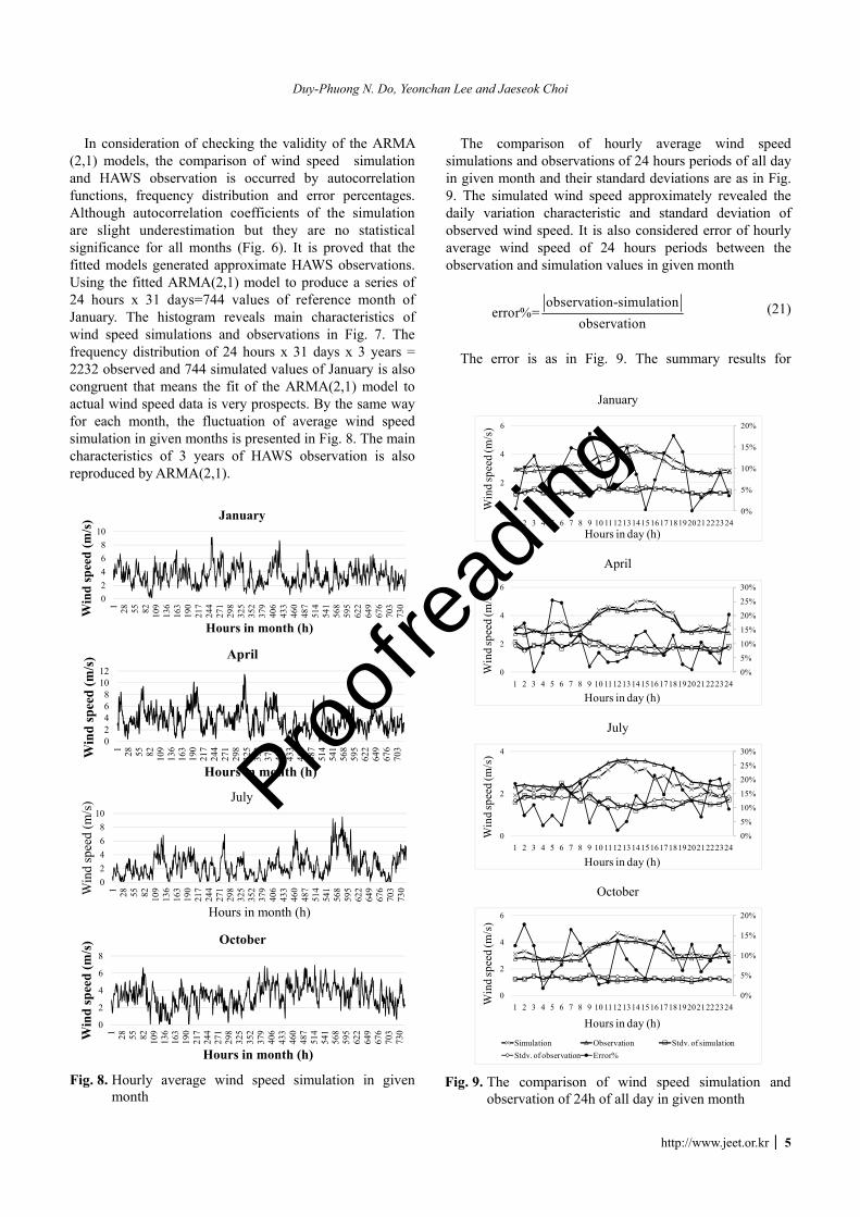
In consideration of checking the validity of the ARMA (2,1) models, the comparison of wind speed simulation and HAWS observation is occurred by autocorrelation functions, frequency distribution and error percentages. Although autocorrelation coefficients of the simulation are slight underestimation but they are no statistical significance for all months (Fig. 6). It is proved that the fitted models generated approximate HAWS observations. Using the fitted ARMA(2,1) model to produce a series of 24 hours x 31 days=744 values of reference month of January. The histogram reveals main characteristics of wind speed simulations and observations in Fig. 7. The frequency distribution of 24 hours x 31 days x 3 years = 2232 observed and 744 simulated values of January is also congruent that means the fit of the ARMA(2,1) model to actual wind speed data is very prospects. By the same way for each month, the fluctuation of average wind speed simulation in given months is presented in Fig. 8. The main characteristics of 3 years of HAWS observation is also reproduced by ARMA(2,1).

Fig. 8. Hourly average wind speed simulation in given

month

The comparison of hourly average wind speed simulations and observations of 24 hours periods of all day in given month and their standard deviations are as in Fig. 9. The simulated wind speed approximately revealed the daily variation characteristic and standard deviation of observed wind speed. It is also considered error of hourly average wind speed of 24 hours periods between the observation and simulation values in given month

observation-simulationerror%=

observation (21)

The error is as in Fig. 9. The summary results for

02468

10

1 28 55 82 109

136

163

190

217

244

271

298

325

352

379

406

433

460

487

514

541

568

595

622

649

676

703

730Win

d sp

eed

(m/s

)

Hours in month (h)

January

02468

1012

1 28 55 82 109

136

163

190

217

244

271

298

325

352

379

406

433

460

487

514

541

568

595

622

649

676

703W

ind

spee

d (m

/s)

Hours in month (h)

April

02468

10

1 28 55 82 109

136

163

190

217

244

271

298

325

352

379

406

433

460

487

514

541

568

595

622

649

676

703

730W

ind

spee

d (m

/s)

Hours in month (h)

July

0

2

4

6

8

1 28 55 82 109

136

163

190

217

244

271

298

325

352

379

406

433

460

487

514

541

568

595

622

649

676

703

730W

ind

spee

d (m

/s)

Hours in month (h)

October

January

April

July

October

Fig. 9. The comparison of wind speed simulation and

observation of 24h of all day in given month

0%

5%

10%

15%

20%

0

2

4

6

1 2 3 4 5 6 7 8 9 10 1112131415161718192021222324

Win

d sp

eed

(m/s

)

Hours in day (h)

0%

5%

10%

15%

20%

25%

30%

0

2

4

6

1 2 3 4 5 6 7 8 9 10 1112131415161718192021222324

Win

d sp

eed

(m/s

)

Hours in day (h)

0%

5%

10%

15%

20%

25%

30%

0

2

4

1 2 3 4 5 6 7 8 9 10 1112131415161718192021222324

Win

d sp

eed

(m/s

)

Hours in day (h)

0%

5%

10%

15%

20%

0

2

4

6

1 2 3 4 5 6 7 8 9 10 1112131415161718192021222324Win

d sp

eed

(m/s

)

Hours in day (h)Simulation Observation Stdv. of simulationStdv. of observation Error%

Proofreading

Hourly Average Wind Speed Simulation and Forecast Based on ARMA Model in Jeju Island, Korea

6 │ J Electr Eng Technol.2016; 11(?): 00-00

synthetic sequences are presented in Table 3. From the above analysis and results of Table 2 shows that observation (obs) and simulation (sim) of hourly wind speed are satisfactory. The simulations of generating all months represent the approximate real statistical characteristics of 3 years of HAWS data in Jeju Island, Korea.

5. Ahead of a Day Wind Speed Forecast The simulated ARMA(2,1) model is also used to forecast

hourly average wind speed in Jeju Island by the weighted sum of previous wind speed values [2]. The predicted wind speed is expressed as

π π ⋯ π 22

where π weights are obtained by inverted form of the ARMA(2,1) model

π π 1,2, … , 23

Because the π weights series is declined sharply, the

accuracy of predicted values is sufficient in moderate n previous values. The predicted wind speed with 24 lead time hours 24 is showed in Fig. 10, as example for March 7th, 2015. The wind speed forecast decays exponentially to mean value in long lead time. The error of wind speed forecast 24 is randomly fluctuation in acceptable range, exception of too low and suddenly varied values. Almost actual wind speed is on 95% probability limits of , which is variance of the wind speed forecast errors.

However, the uncorrelated wind speed forecast errors are decayed at longer lead times l. It is need to use ψ weights series for updating the old predicted values at origin time t and lead time l+k by new ones at origin time t+k and lead time l [2]

Fig. 10. The wind speed forecast in March 7th, 2015

ψ k 24

where ψ ψ ψ 1,2, … , and ψ = 1, ψ = 0 for l < 0 and = 0 for l > 1.

In this case, the predicted wind speed is updated in every hour 1 . The updated wind speed forecast sticks to the actual wind speed well (Fig. 10).

6. Conclusion The HAWS data, which is transformed to stationary

variable, is analyzed by Box – Jenkins methodology to build up wind speed models. Many subclass of ARMA(p,q) model is considered by autocorrelation, partial auto-correlation function and BIC criterion analysis to select the fitted models. Finally, in parameters estimating and diagnostic checking stage, ARMA(2,1) models are proposed for all months. The comparison between the observations and the simulations of autocorrelation function, frequency distribution and main statistical characteristics of demonstrates the models are fitted. These ARMA(2,1) models are used to generate reference monthly data which close to the actual statistical characteristics of the 3 year (from 2010 to 2012) time series of wind speed data in Jeju Island. These models are also developed to build up forecast model of wind speed in Jeju Island. In short-term, the wind speed forecast values are acceptable and keep on main characteristics of the models. It is useful tool for studying more in reliability analysis of power system including wind power in Jeju Island, Korea.

Acknowledgements This work was supported by the Korean National Re-

search Foundation (No. #2012R1A2A2A01012803)

References

[1] B. Brown, R. Katz. and A. Murphy, “Times Series Models to Simulate and Forecast Wind Speed and

0%

30%

60%

90%

120%

150%

02468

10

1 3 5 7 9 11 13 15 17 19 21 23

Err

or (%

)

Lead time (h)Vpredicted(24) Vupdated(1) VactualV(+) 95% limit V(-) 95% limit Verror(24)

Table 3. Statistics for Observed (Obs) and Simulated (Sim) HAWS in Jeju Island

Month Mean (m/s) Variance (m/s)2 Sim Obs Error% Sim Obs Error%

Jan 3.44 3.16 8.7% 2.19 2.17 1.1% Feb 2.86 3.09 7.2% 1.99 2.36 15.4%Mar 3.74 3.65 2.6% 2.72 3.06 10.8%Apr 3.70 3.38 9.3% 3.65 3.71 1.7% May 3.10 2.99 3.4% 3.11 3.11 0.2% Jun 2.72 2.72 0.2% 3.03 3.10 2.2% Jul 2.49 2.82 11.8% 2.92 3.15 7.2%

Aug 3.77 3.49 7.9% 5.01 6.59 24.0%Sep 3.34 3.18 5.2% 3.14 3.27 3.8% Oct 3.43 3.14 9.3% 1.77 2.04 13.5%Nov 2.65 3.02 12.2% 1.92 2.35 18.3%Dec 2.96 3.13 5.5% 2.03 2.61 22.2%

Proofreading

Duy-Phuong N. Do, Yeonchan Lee and Jaeseok Choi

http://www.jeet.or.kr │ 7

Wind Power”, Climate and applied meteorology, vol. 23, 1984

[2] Box P. and Jenkins M., Times Series Analysis, Forecasting and Control, Holden-Day, San Franc, 1976

[3] H. Nfaoui, and M. Sayigh, “Stochastic Simulation of Hourly Wind Speed Sequences in Tangiers”, Solar Energy, vol. 56, no. 3, pp. 301-314, 1996

[4] K. Philippopoulos and D. Deligiorgi, “Statistical Simulation of Wind Speed in Athens, Greece Based on Weibull and ARMA Models” International Journal of Energy and Environment, issue.4, vol. 3, 2009

[5] P. Box, G. Cox, “An Analysis of Transformations”, Jour. Royal Sta. Sco., B26, 211, 1964

[6] R. Karki, P. Hu and R. Billinton, “A simplified wind power generation model for reliability evaluation” IEEE Trans. Energy Conversion, vol. 21, no. 2, 2006.

[7] D. R. Chandra, M. S. Kumari, M. Sydulu, F. Grimaccia and M. Mussetta, “Adaptive wavelet neural network based wind speed forecasting studies” JEET, vol. 9, no. 6, pp. 1812-1821, 2014

[8] Dániel Divényi, János Divényi, “Wind Speed Simul-ator Base on Wind Generation Using Autoregressive Statistical Model”, Electrotehnică, Electronică, Automatică, nr.2, 2012

[9] A. Kamjoo, A. Maheri, and G. Putrus, “Wind speed and solar irradiance variation simulation using ARMA models in design of hydrid wind-PV-battery system”, Journal of clean energy technologies, vol. 1, no. 1, 2013

[10] Lisa M. Bramer, Thesis: Method for modeling and forecasting wind characteristics, Iowa University, 2013

[11] M. Lei, L. Shiyuan, J. Chuanwen, L. Hongling, Z. Yan, “A Review on the Forecasting of Wind Speed And Generated Power”, Renewable and Sustainable Energy Reviews, 2009

Duy-Phuong N.Do He was born in Can Tho city, VietNam in 1982. He received B.S and M.Sc degree in electrical engineering from CanTho University and HoChiMinh University of Technology, respectively. His re-search interest is stability evaluation of power system. Now, he is studying as

Ph.D student in Gyeongsang National University.

Yeonchan Lee He was born in Gosung, Korea in 1987. His research interest includes Transmission Expansion Plan-ning using Reliability Evaluation of Power Systems. He received the B.Sc. degree from Gyeongsang National University in 2013.

Jaeseok Choi He was born in Kyeongju, Korea, in 1958. He received the B.Sc., M.Sc., and Ph.D. degrees from Korea University, Seoul. Since 1991, he has been on the faculty of Gyeongsang National University, Jinju, Korea, where he is a professor. He was a visiting professor at Cornell

University, Ithaca, NY, USA, in 2004. He is also adjunct professor at IIT, IL, USA since 2007. His research interests include fuzzy applications, probabilistic production cost simulation, reliability evaluation, and outage cost assess-ment of power systems.

Proofreading