Item Response TheoryUsing

Bayesian Networks

by

Richard Neapolitan

I will follow the Bayesian network approach to IRT forwarded by Almond and Mislevy:

http://ecd.ralmond.net/tutorial/

A good tutorial that introduces basic IRT is provided at the following site:

http://www.creative-wisdom.com/multimedia/ICHA.htm

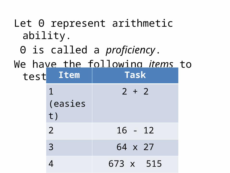
Let Θ represent arithmetic ability. Θ is called a proficiency.We have the following items to test Θ:

Item Task

1 (easiest) 2 + 2

2 16 - 12

3 64 x 27

4 673 x 515

5 (hardest) 105,110 / 67

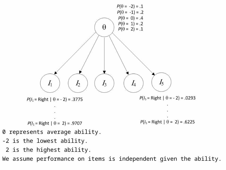
0 represents average ability.-2 is the lowest ability. 2 is the highest ability.We assume performance on items is independent given the ability.

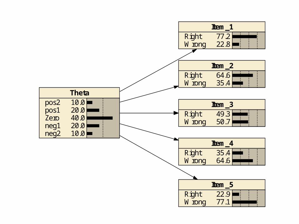
Thetapos2pos1Zeroneg1neg2

10.020.040.020.010.0

Item_4RightWrong

35.464.6

Item_3RightWrong

49.350.7

Item_2RightWrong

64.635.4

Item_1RightWrong

77.222.8

Item_5RightWrong

22.977.1

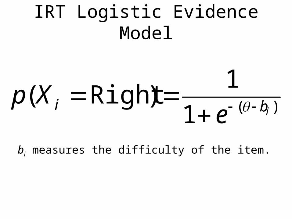
IRT Logistic Evidence Model

bi measures the difficulty of the item.

)(1

1)Right(

ibi eXp

b = 0 (average difficulty)

-5 -4 -3 -2 -1 0 1 2 3 4 5

0.1

0.2

0.3

0.4

0.5

0.6

0.7

0.8

0.9

1.0

theta

P

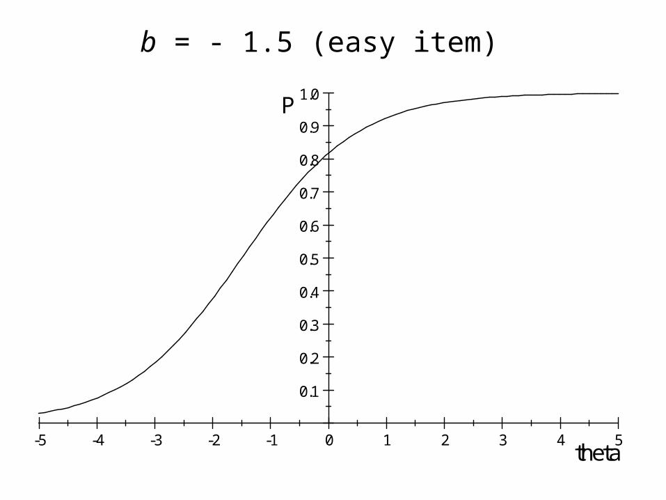
b = - 1.5 (easy item)

-5 -4 -3 -2 -1 0 1 2 3 4 5

0.1

0.2

0.3

0.4

0.5

0.6

0.7

0.8

0.9

1.0

theta

P

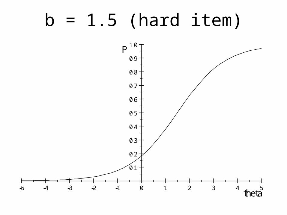
b = 1.5 (hard item)

-5 -4 -3 -2 -1 0 1 2 3 4 5

0.1

0.2

0.3

0.4

0.5

0.6

0.7

0.8

0.9

1.0

theta

P

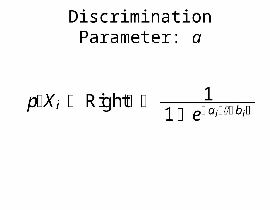
Discrimination Parameter: a

pXi Right 11 e a i b i

a = 5, b = 0

-5 -4 -3 -2 -1 0 1 2 3 4 5

0.1

0.2

0.3

0.4

0.5

0.6

0.7

0.8

0.9

1.0

theta

P

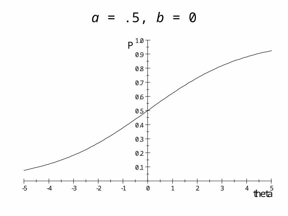
a = .5, b = 0

-5 -4 -3 -2 -1 0 1 2 3 4 5

0.1

0.2

0.3

0.4

0.5

0.6

0.7

0.8

0.9

1.0

theta

P

a = 5, b = 1.5

-5 -4 -3 -2 -1 0 1 2 3 4 5

0.1

0.2

0.3

0.4

0.5

0.6

0.7

0.8

0.9

1.0

theta

P

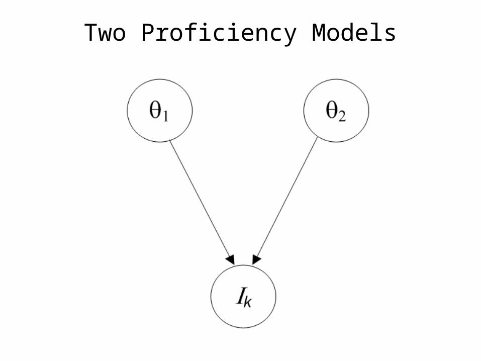
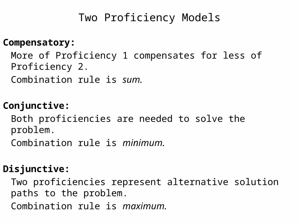
Two Proficiency Models

Two Proficiency Models

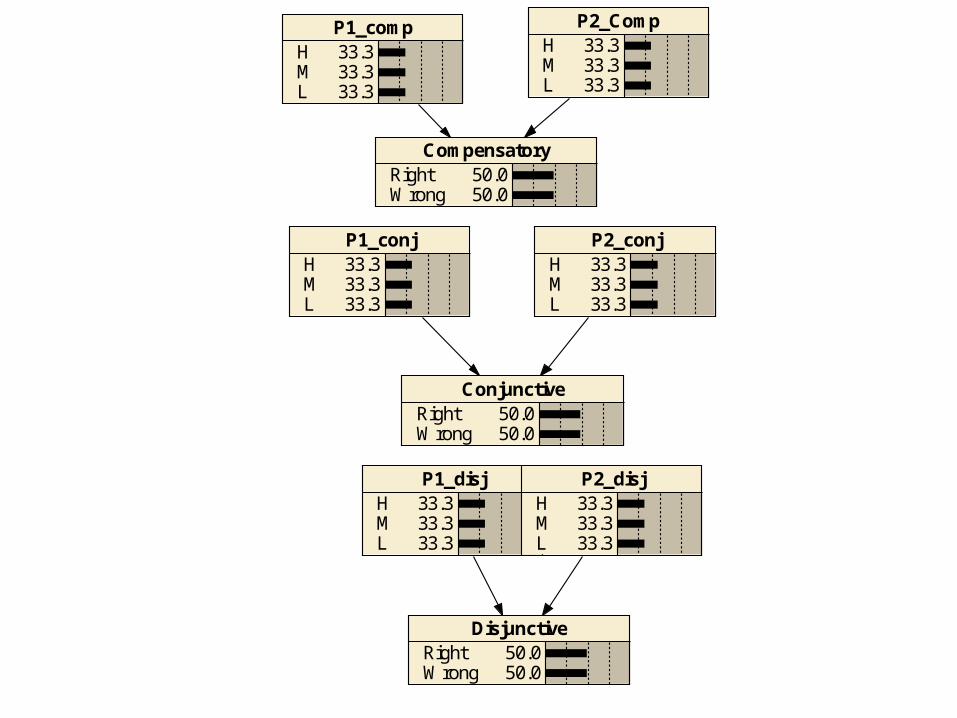
Compensatory: More of Proficiency 1 compensates for less of Proficiency 2.Combination rule is sum.

Conjunctive: Both proficiencies are needed to solve the problem.Combination rule is minimum.

Disjunctive: Two proficiencies represent alternative solution paths to the problem.Combination rule is maximum.

P1_disjHML

33.333.333.3

P2_disjHML

33.333.333.3

DisjunctiveRightWrong

50.050.0

ConjunctiveRightWrong

50.050.0

P1_conjHML

33.333.333.3

P1_compHML

33.333.333.3

CompensatoryRightWrong

50.050.0

P2_CompHML

33.333.333.3

P2_conjHML

33.333.333.3

Task3

RightWrong

50.050.0

0.5 ± 0.5

Skill2

YesNo

50.050.0

0.5 ± 0.5

Skill1

YesNo

50.050.0

0.5 ± 0.5

Task1

RightWrong

50.050.0

0.5 ± 0.5

Task2

RightWrong

50.050.0

0.5 ± 0.5

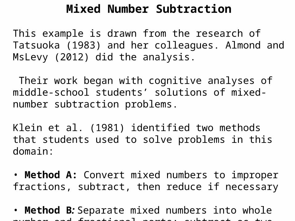
Mixed Number Subtraction

This example is drawn from the research of Tatsuoka (1983) and her colleagues. Almond and MsLevy (2012) did the analysis.

Their work began with cognitive analyses of middle-school students’ solutions of mixed-number subtraction problems.

Klein et al. (1981) identified two methods that students used to solve problems in this domain:

• Method A: Convert mixed numbers to improper fractions, subtract, then reduce if necessary

• Method B: Separate mixed numbers into whole number and fractional parts; subtract as two subproblems, borrowing one from minuend whole number if necessary; then simplify and reduce if necessary.

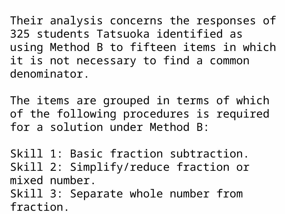
Their analysis concerns the responses of 325 students Tatsuoka identified as using Method B to fifteen items in which it is not necessary to find a common denominator.

The items are grouped in terms of which of the following procedures is required for a solution under Method B:

Skill 1: Basic fraction subtraction.Skill 2: Simplify/reduce fraction or mixed number.Skill 3: Separate whole number from fraction.Skill 4: Borrow one from the whole number in a given mixed number.Skill 5: Convert a whole number to a fraction.

All models are conjunctive.

Learning Parameters From Data

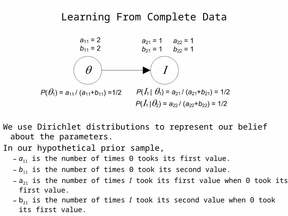
Learning From Complete Data

We use Dirichlet distributions to represent our belief about the parameters.

In our hypothetical prior sample,– a11 is the number of times Θ tooks its first value.

– b11 is the number of times Θ took its second value.

– a21 is the number of times I took its first value when Θ took its first value.

– b21 is the number of times I took its second value when Θ took its first value.

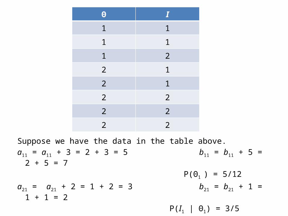
Suppose we have the data in the table above.a11 = a11 + 3 = 2 + 3 = 5 b11 = b11 + 5 = 2 + 5 = 7

P(Θ1 ) = 5/12

a21 = a21 + 2 = 1 + 2 = 3 b21 = b21 + 1 = 1 + 1 = 2

P(I1 | Θ1) = 3/5

Θ I

1 1

1 1

1 2

2 1

2 1

2 2

2 2

2 2

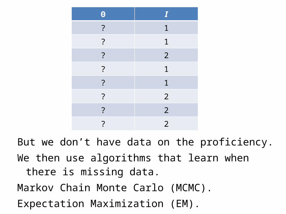
But we don’t have data on the proficiency.We then use algorithms that learn when there is

missing data.Markov Chain Monte Carlo (MCMC).Expectation Maximization (EM).

Θ I

? 1

? 1

? 2

? 1

? 1

? 2

? 2

? 2

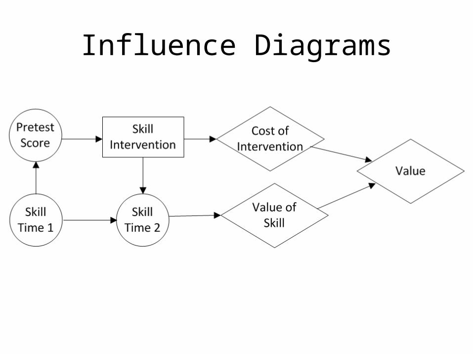
Influence Diagrams

Standard IRT

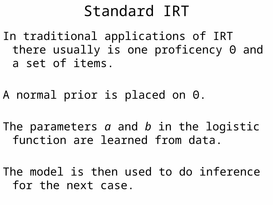
In traditional applications of IRT there usually is one proficency Θ and a set of items.

A normal prior is placed on Θ.

The parameters a and b in the logistic function are learned from data.

The model is then used to do inference for the next case.