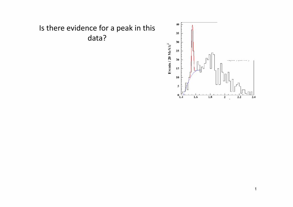
Is there evidence for a peak in this data? - PPD · Data statistic, selections, corrections, method...
61
1 Is there evidence for a peak in this data?
Transcript of Is there evidence for a peak in this data? - PPD · Data statistic, selections, corrections, method...
1
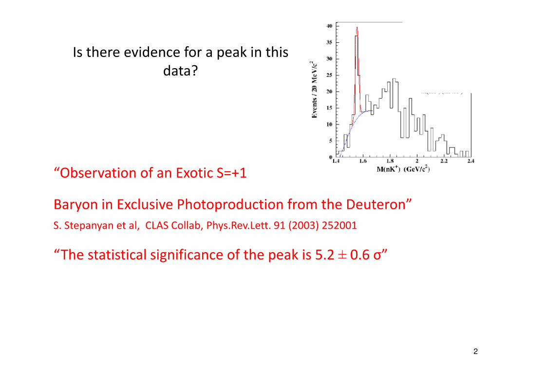
Is there evidence for a peak in this
data?
2
“Observation of an Exotic S=+1
Baryon in Exclusive Photoproduction from the Deuteron”
S. Stepanyan et al, CLAS Collab, Phys.Rev.Lett. 91 (2003) 252001
“The statistical significance of the peak is 5.2 ± 0.6 σ”
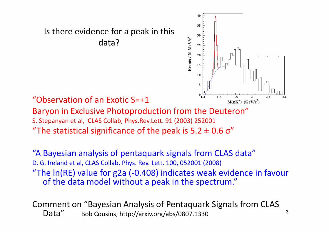
Is there evidence for a peak in this
data?
3
“Observation of an Exotic S=+1
Baryon in Exclusive Photoproduction from the Deuteron” S. Stepanyan et al, CLAS Collab, Phys.Rev.Lett. 91 (2003) 252001
“The statistical significance of the peak is 5.2 ± 0.6 σ”
“A Bayesian analysis of pentaquark signals from CLAS data”D. G. Ireland et al, CLAS Collab, Phys. Rev. Lett. 100, 052001 (2008)
“The ln(RE) value for g2a (-0.408) indicates weak evidence in favour of the data model without a peak in the spectrum.”
Comment on “Bayesian Analysis of Pentaquark Signals from CLAS Data” Bob Cousins, http://arxiv.org/abs/0807.1330
Is there evidence for a peak in this
data?
Statistical Issues in Searches for
New Physics
Louis Lyons
Imperial College, London
and
Oxford
RAL
October 2016
4
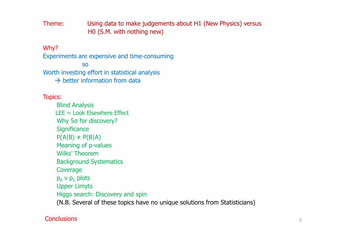
Theme: Using data to make judgements about H1 (New Physics) versus
H0 (S.M. with nothing new)
Why?
Experiments are expensive and time-consuming
so
Worth investing effort in statistical analysis
� better information from data
Topics:
Blind AnalysisLEE = Look Elsewhere Effect
Why 5σ for discovery?
Significance
P(A|B) ≠ P(B|A)
Meaning of p-values
Wilks’ Theorem
Background Systematics
Coverage
p0 v p1 plots
Upper Limyts
Higgs search: Discovery and spin
(N.B. Several of these topics have no unique solutions from Statisticians)
Conclusions 5
6
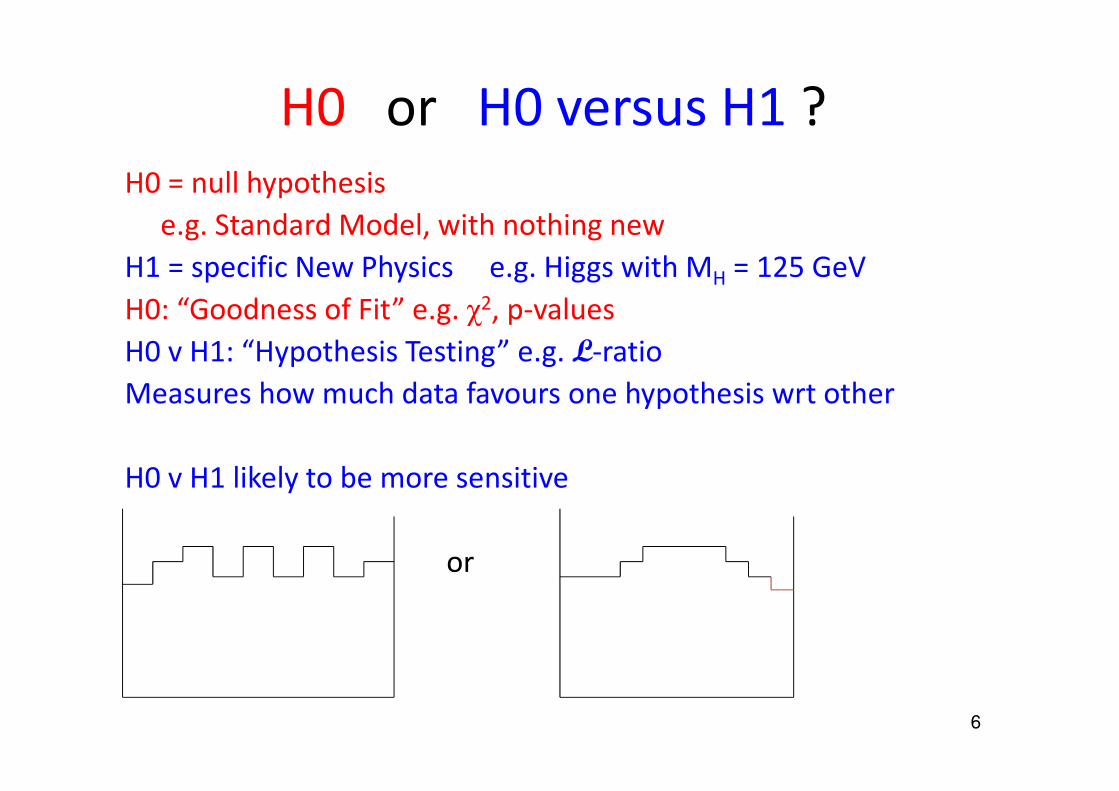
H0 or H0 versus H1 ?
H0 = null hypothesis
e.g. Standard Model, with nothing new
H1 = specific New Physics e.g. Higgs with MH = 125 GeV
H0: “Goodness of Fit” e.g. χ2, p-values
H0 v H1: “Hypothesis Testing” e.g. L-ratio
Measures how much data favours one hypothesis wrt other
H0 v H1 likely to be more sensitive
or

7
Examples of Hypotheses1) Event selector (Event = particle interaction)Events produced at CERN LHC at enormous rateOnline ‘trigger’ to select events for recording (~1 kiloHertz)
e.g. events with many particlesOffline selection based on required features
e.g. H0: At least 2 muons H1: 0 or 1 muonPossible outcomes: Events assigned as H0 or H1
2) Result of experiment e.g. H0 = nothing new, just b
H1 = new particle produced as well, b+s(Higgs, SUSY, 4th neutrino,…..)
Possible outcomes H0 H1� X Exclude H1X � Discovery� � No decisionX X ?
.

8
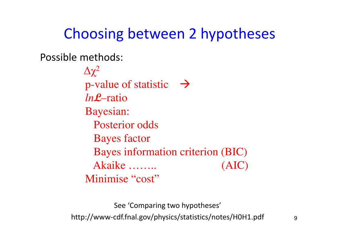
Choosing between 2 hypotheses
Hypothesis testing: New particle or statistical fluctuation?H0 = b H1 = b + s
9
Choosing between 2 hypotheses
Possible methods:
∆χ2
p-value of statistic �
lnL–ratio
Bayesian:
Posterior odds
Bayes factor
Bayes information criterion (BIC)
Akaike …….. (AIC)
Minimise “cost”
See ‘Comparing two hypotheses’
http://www-cdf.fnal.gov/physics/statistics/notes/H0H1.pdf
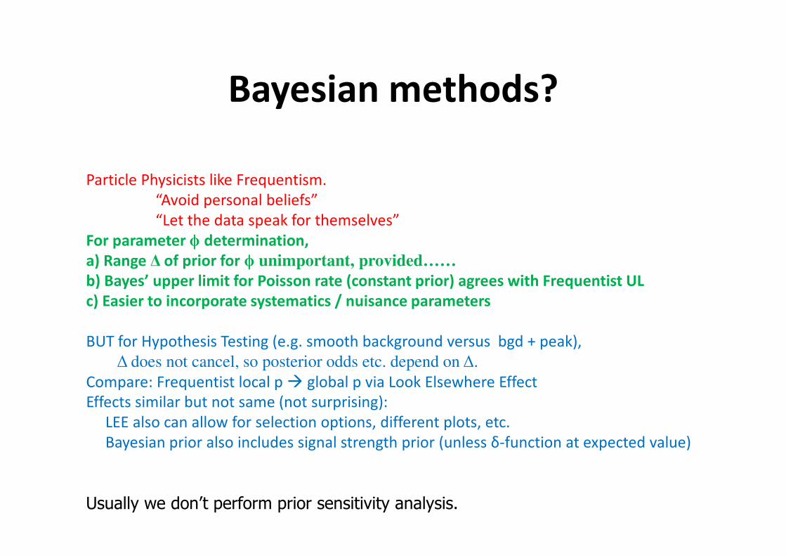
Bayesian methods?
Particle Physicists like Frequentism.
“Avoid personal beliefs”
“Let the data speak for themselves”
For parameter ϕ determination,
a) Range ∆ of prior for ϕ unimportant, provided……
b) Bayes’ upper limit for Poisson rate (constant prior) agrees with Frequentist UL
c) Easier to incorporate systematics / nuisance parameters
BUT for Hypothesis Testing (e.g. smooth background versus bgd + peak),
∆ does not cancel, so posterior odds etc. depend on ∆.
Compare: Frequentist local p � global p via Look Elsewhere Effect
Effects similar but not same (not surprising):
LEE also can allow for selection options, different plots, etc.
Bayesian prior also includes signal strength prior (unless δ-function at expected value)
Usually we don’t perform prior sensitivity analysis.
11
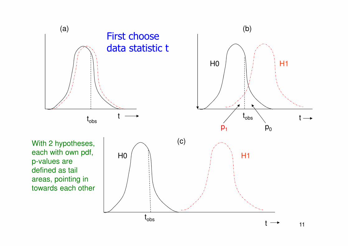
(a) (b)
(c)
H0 H1
p1 p0
t
t ttobstobs
tobs
H0 H1
With 2 hypotheses, each with own pdf, p-values are defined as tail areas, pointing in towards each other
First choose data statistic t
12
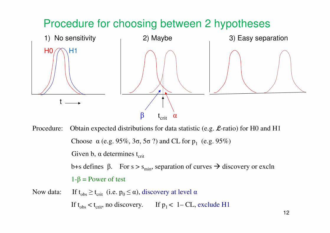
1) No sensitivity 2) Maybe 3) Easy separation
H0 H1
t
β tcrit α
Procedure: Obtain expected distributions for data statistic (e.g. L-ratio) for H0 and H1
Choose α (e.g. 95%, 3σ, 5σ ?) and CL for p1 (e.g. 95%)
Given b, α determines tcrit
b+s defines β. For s > smin, separation of curves � discovery or excln
1-β = Power of test
Now data: If tobs ≥ tcrit (i.e. p0 ≤ α), discovery at level α
If tobs < tcrit, no discovery. If p1 < 1– CL, exclude H1
Procedure for choosing between 2 hypotheses

Slide 12
N1 NPL, 06/11/2005
13
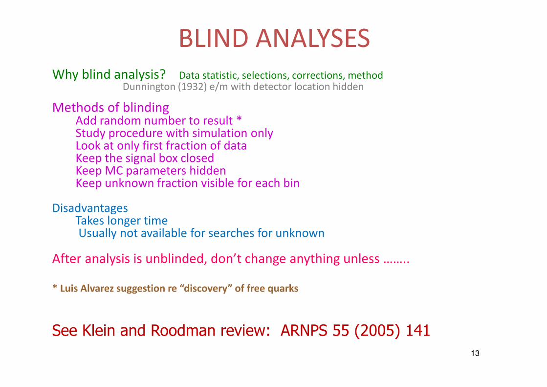
BLIND ANALYSESWhy blind analysis? Data statistic, selections, corrections, method
Dunnington (1932) e/m with detector location hidden
Methods of blindingAdd random number to result *Study procedure with simulation onlyLook at only first fraction of dataKeep the signal box closedKeep MC parameters hiddenKeep unknown fraction visible for each bin
DisadvantagesTakes longer timeUsually not available for searches for unknown
After analysis is unblinded, don’t change anything unless ……..
* Luis Alvarez suggestion re “discovery” of free quarks
See Klein and Roodman review: ARNPS 55 (2005) 141
14
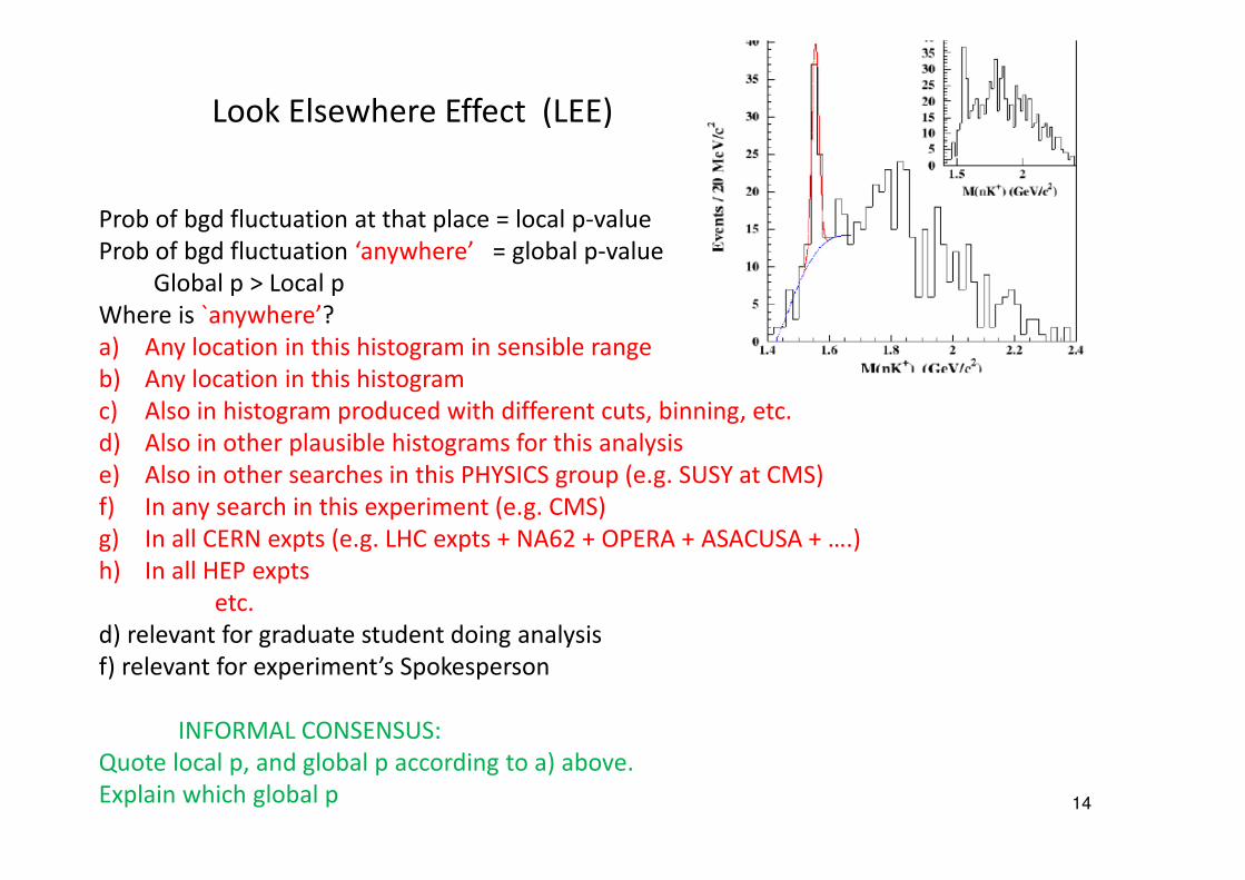
Look Elsewhere Effect (LEE)
Prob of bgd fluctuation at that place = local p-value
Prob of bgd fluctuation ‘anywhere’ = global p-value
Global p > Local p
Where is `anywhere’?
a) Any location in this histogram in sensible range
b) Any location in this histogram
c) Also in histogram produced with different cuts, binning, etc.
d) Also in other plausible histograms for this analysis
e) Also in other searches in this PHYSICS group (e.g. SUSY at CMS)
f) In any search in this experiment (e.g. CMS)
g) In all CERN expts (e.g. LHC expts + NA62 + OPERA + ASACUSA + ….)
h) In all HEP expts
etc.
d) relevant for graduate student doing analysis
f) relevant for experiment’s Spokesperson
INFORMAL CONSENSUS:
Quote local p, and global p according to a) above.
Explain which global p
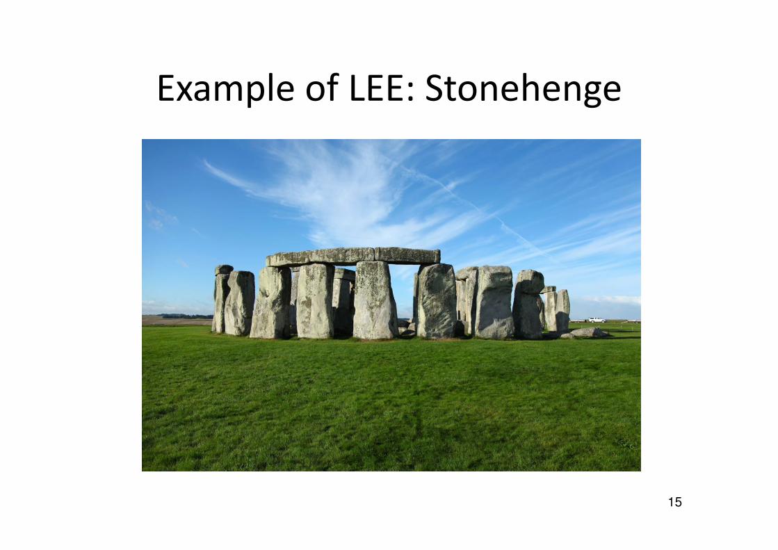
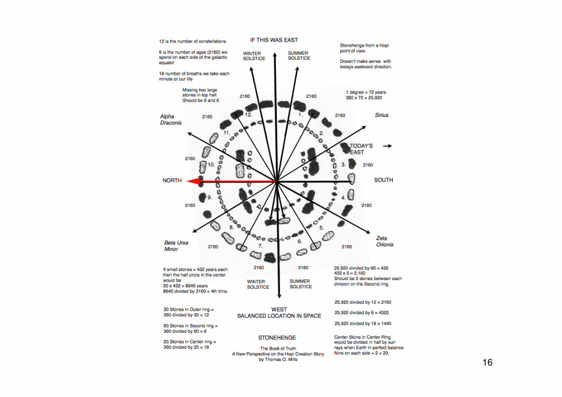
Example of LEE: Stonehenge
15
16
Are alignments significant?
• Atkinson replied with his article "Moonshine on Stonehenge" in Antiquity in 1966, pointing out that some of the pits which ….. had used for his sight lines were more likely to have been natural depressions, and that he had allowed a margin of error of up to 2 degrees in his alignments. Atkinson found that the probability of so many alignments being visible from 165 points to be close to 0.5 rather that the "one in a million" possibility which ….. had claimed.
• ….. had been examining stone circles since the 1950s in search of astronomical alignments and the megalithic yard. It was not until 1973 that he turned his attention to Stonehenge. He chose to ignore alignments between features within the monument, considering them to be too close together to be reliable. He looked for landscape features that could have marked lunar and solar events. However, one of …..'s key sites, Peter's Mound, turned out to be a twentieth-century rubbish dump.
17
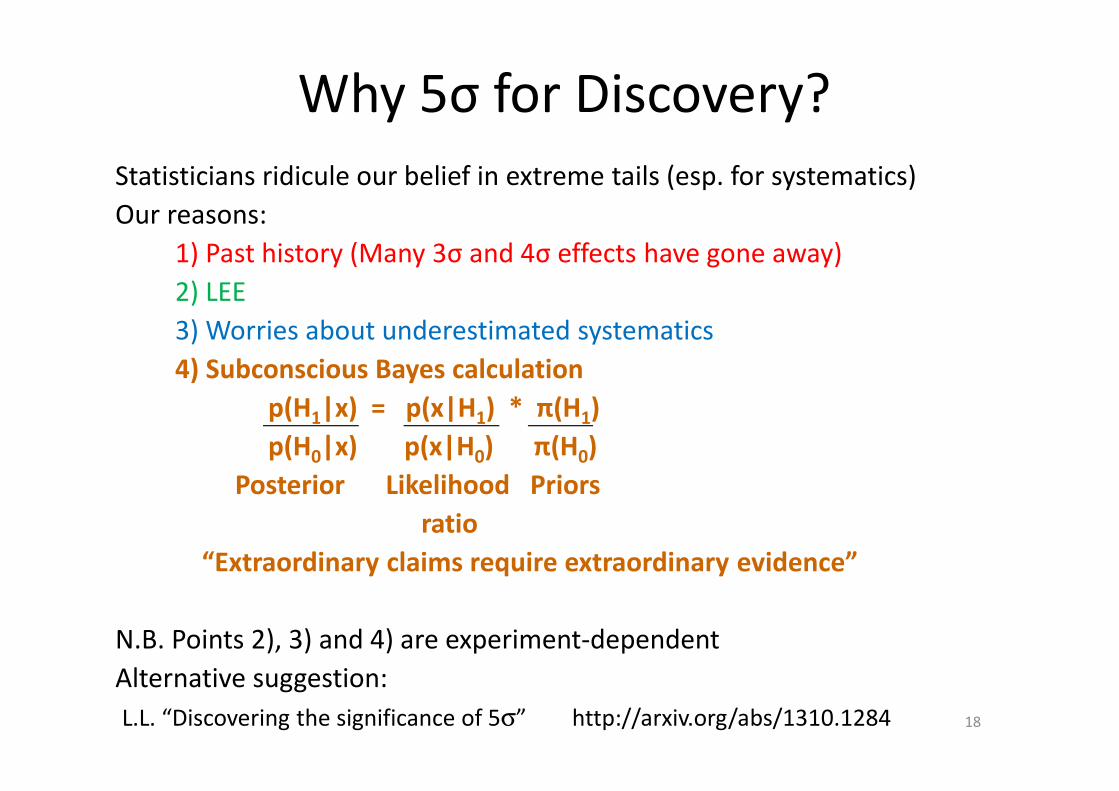
Why 5σ for Discovery?
Statisticians ridicule our belief in extreme tails (esp. for systematics)
Our reasons:
1) Past history (Many 3σ and 4σ effects have gone away)
2) LEE
3) Worries about underestimated systematics
4) Subconscious Bayes calculation
p(H1|x) = p(x|H1) * π(H1)
p(H0|x) p(x|H0) π(H0)
Posterior Likelihood Priors
ratio
“Extraordinary claims require extraordinary evidence”
N.B. Points 2), 3) and 4) are experiment-dependent
Alternative suggestion:
L.L. “Discovering the significance of 5σ” http://arxiv.org/abs/1310.1284 18
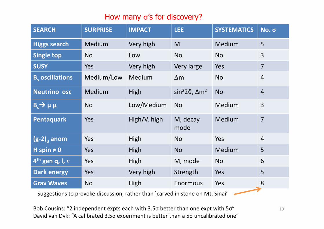
SEARCH SURPRISE IMPACT LEE SYSTEMATICS No. σ
Higgs search Medium Very high M Medium 5
Single top No Low No No 3
SUSY Yes Very high Very large Yes 7
Bs oscillations Medium/Low Medium ∆m No 4
Neutrino osc Medium High sin22ϑ, Δm2 No 4
Bs���� μ μ No Low/Medium No Medium 3
Pentaquark Yes High/V. high M, decay
mode
Medium 7
(g-2)μ anom Yes High No Yes 4
H spin ≠ 0 Yes High No Medium 5
4th gen q, l, ν Yes High M, mode No 6
Dark energy Yes Very high Strength Yes 5
Grav Waves No High Enormous Yes 8
19
Suggestions to provoke discussion, rather than `carved in stone on Mt. Sinai’
Bob Cousins: “2 independent expts each with 3.5σ better than one expt with 5σ”
David van Dyk: “A calibrated 3.5σ experiment is better than a 5σ uncalibrated one”
How many σ’s for discovery?
20
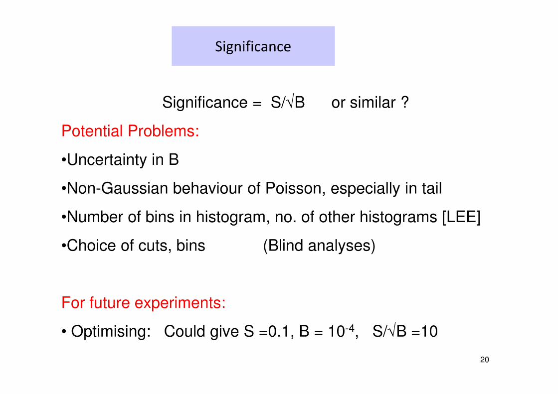
Significance
Significance = S/√B or similar ?
Potential Problems:
•Uncertainty in B
•Non-Gaussian behaviour of Poisson, especially in tail
•Number of bins in histogram, no. of other histograms [LEE]
•Choice of cuts, bins (Blind analyses)
For future experiments:
• Optimising: Could give S =0.1, B = 10-4, S/√B =10
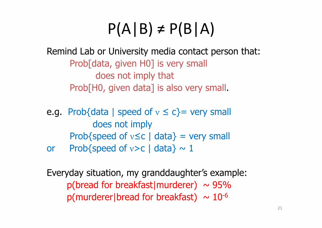
P(A|B) ≠ P(B|A)
Remind Lab or University media contact person that:
Prob[data, given H0] is very small
does not imply that
Prob[H0, given data] is also very small.
e.g. Prob{data | speed of ν ≤ c}= very small
does not imply
Prob{speed of ν≤c | data} = very small
or Prob{speed of ν>c | data} ~ 1
Everyday situation, my granddaughter’s example:
p(bread for breakfast|murderer) ~ 95%
p(murderer|bread for breakfast) ~ 10-6
21
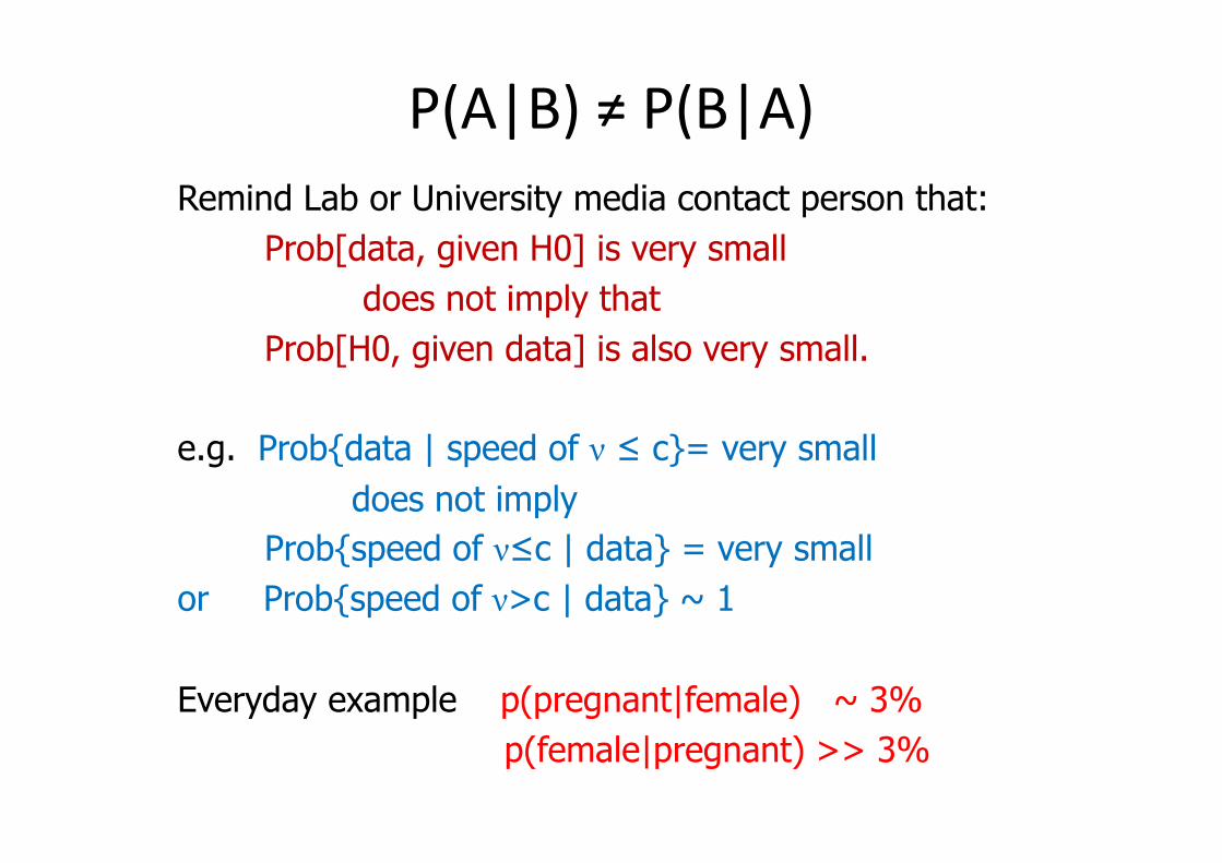
P(A|B) ≠ P(B|A)
Remind Lab or University media contact person that:
Prob[data, given H0] is very small
does not imply that
Prob[H0, given data] is also very small.
e.g. Prob{data | speed of ν ≤ c}= very small
does not imply
Prob{speed of ν≤c | data} = very small
or Prob{speed of ν>c | data} ~ 1
Everyday example p(pregnant|female) ~ 3%
p(female|pregnant) >> 3%
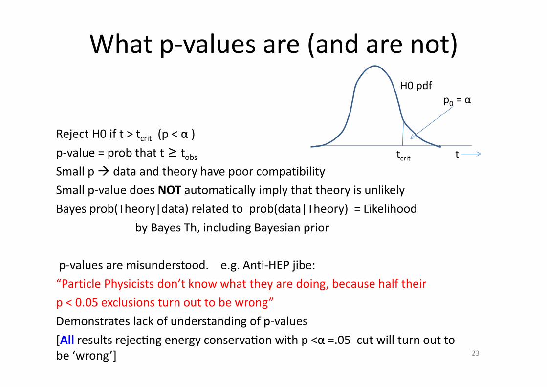
What p-values are (and are not)
Reject H0 if t > tcrit (p < α )
p-value = prob that t ≥ tobs
Small p � data and theory have poor compatibility
Small p-value does NOT automatically imply that theory is unlikely
Bayes prob(Theory|data) related to prob(data|Theory) = Likelihood
by Bayes Th, including Bayesian prior
p-values are misunderstood. e.g. Anti-HEP jibe:
“Particle Physicists don’t know what they are doing, because half their
p ˂ 0.05 exclusions turn out to be wrong”
Demonstrates lack of understanding of p-values
[All results rejecZng energy conservaZon with p ˂α =.05 cut will turn out to
be ‘wrong’] 23
H0 pdf
p0 = α
tcrit t
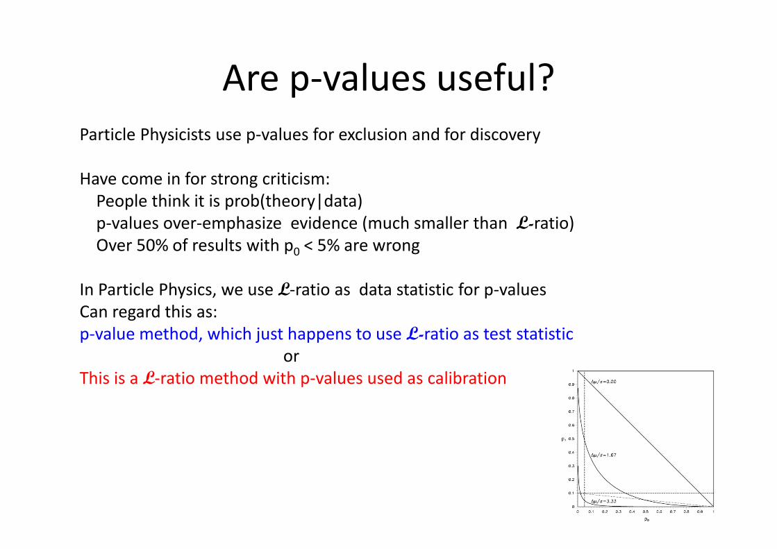
Are p-values useful?
Particle Physicists use p-values for exclusion and for discovery
Have come in for strong criticism:
People think it is prob(theory|data)
p-values over-emphasize evidence (much smaller than L-ratio)
Over 50% of results with p0 < 5% are wrong
In Particle Physics, we use L-ratio as data statistic for p-values
Can regard this as:
p-value method, which just happens to use L-ratio as test statistic
or
This is a L-ratio method with p-values used as calibration
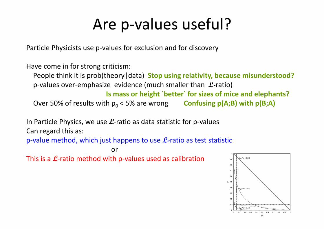
Are p-values useful?
Particle Physicists use p-values for exclusion and for discovery
Have come in for strong criticism:
People think it is prob(theory|data) Stop using relativity, because misunderstood?
p-values over-emphasize evidence (much smaller than L-ratio)
Is mass or height `better` for sizes of mice and elephants?
Over 50% of results with p0 < 5% are wrong Confusing p(A;B) with p(B;A)
In Particle Physics, we use L-ratio as data statistic for p-values
Can regard this as:
p-value method, which just happens to use L-ratio as test statistic
or
This is a L-ratio method with p-values used as calibration
26
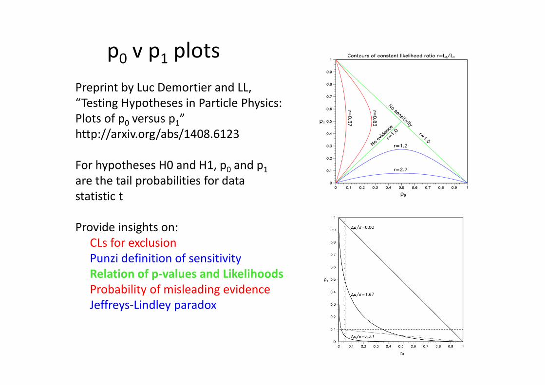
p0 v p1 plots
Preprint by Luc Demortier and LL,
“Testing Hypotheses in Particle Physics:
Plots of p0 versus p1”
http://arxiv.org/abs/1408.6123
For hypotheses H0 and H1, p0 and p1
are the tail probabilities for data
statistic t
Provide insights on:
CLs for exclusion
Punzi definition of sensitivity
Relation of p-values and Likelihoods
Probability of misleading evidence
Jeffreys-Lindley paradox

27
CLs = p1/(1-p0) � diagonal line
Provides protection against excluding H1 when little or no sensitivity
Punzi definition of sensitivity:
Enough separation of pdf’s for no chance of ambiguity
H0 H1
t
Δµ
Can read off power of test
e.g. If H0 is true, what is
prob of rejecting H1?
N.B. p0 = tail towards H1
p1 = tail towards H0
28
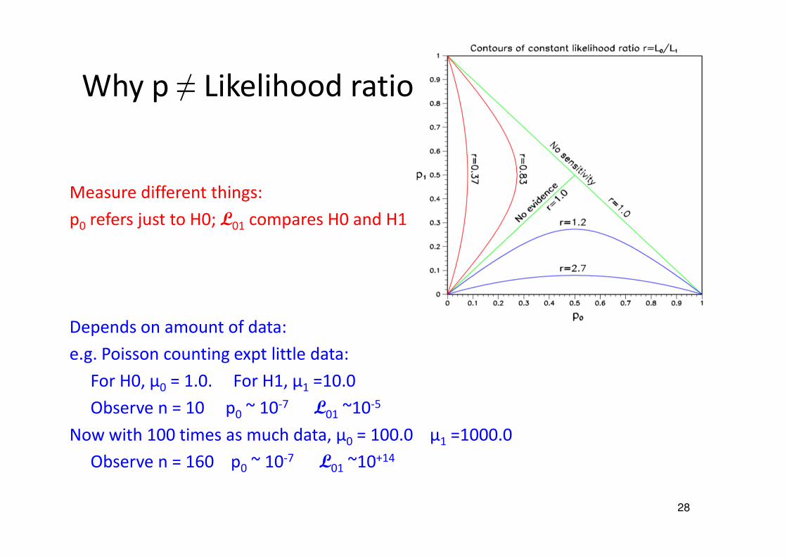
Why p ≠ Likelihood ratio
Measure different things:
p0 refers just to H0; L01 compares H0 and H1
Depends on amount of data:
e.g. Poisson counting expt little data:
For H0, μ0 = 1.0. For H1, μ1 =10.0
Observe n = 10 p0 ~ 10-7 L01 ~10-5
Now with 100 times as much data, μ0 = 100.0 μ1 =1000.0
Observe n = 160 p0 ~ 10-7 L01 ~10+14
29
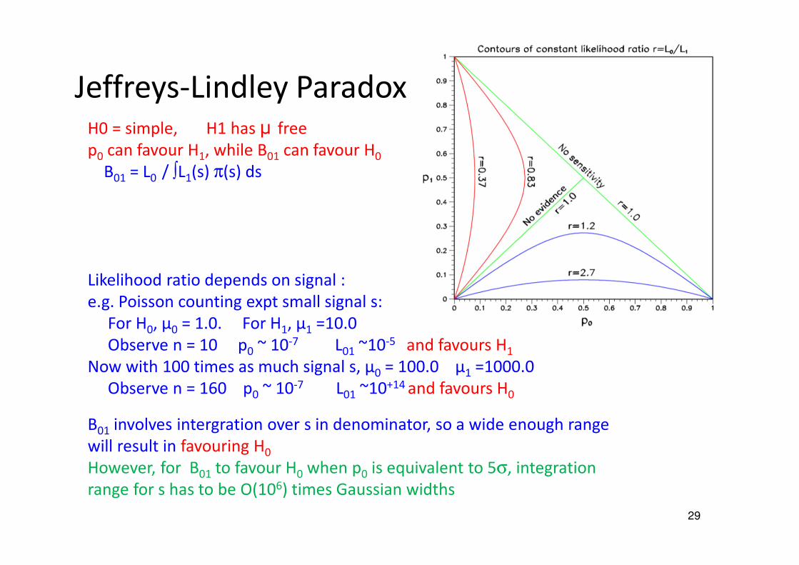
Jeffreys-Lindley ParadoxH0 = simple, H1 has µ free
p0 can favour H1, while B01 can favour H0
B01 = L0 / ∫L1(s) π(s) ds
Likelihood ratio depends on signal :
e.g. Poisson counting expt small signal s:
For H0, μ0 = 1.0. For H1, μ1 =10.0
Observe n = 10 p0 ~ 10-7 L01 ~10-5 and favours H1
Now with 100 times as much signal s, μ0 = 100.0 μ1 =1000.0
Observe n = 160 p0 ~ 10-7 L01 ~10+14 and favours H0
B01 involves intergration over s in denominator, so a wide enough range
will result in favouring H0
However, for B01 to favour H0 when p0 is equivalent to 5σ, integration
range for s has to be O(106) times Gaussian widths
30
Combining different p-values
Several results quote independent p-values for same effect:
p1, p2, p3….. e.g. 0.9, 0.001, 0.3 ……..
What is combined significance? Not just p1*p2*p3…..
If 10 expts each have p ~ 0.5, product ~ 0.001 and is clearly NOT correct combined p
S = z * (-ln z)j /j! , z = p1p2p3…….
(e.g. For 2 measurements, S = z * (1 - lnz) ≥ z )
Problems:
1) Recipe is not unique (Uniform dist in n-D hypercube ���� uniform in 1-D)
2) Formula is not associative
Combining {{p1 and p2}, and then p3} gives different answer
from {{p3 and p2}, and then p1} , or all together
Due to different options for “more extreme than x1, x2, x3”.
3) Small p’s due to different discrepancies
******* Better to combine data ************
∑−
=
1
0
n
j
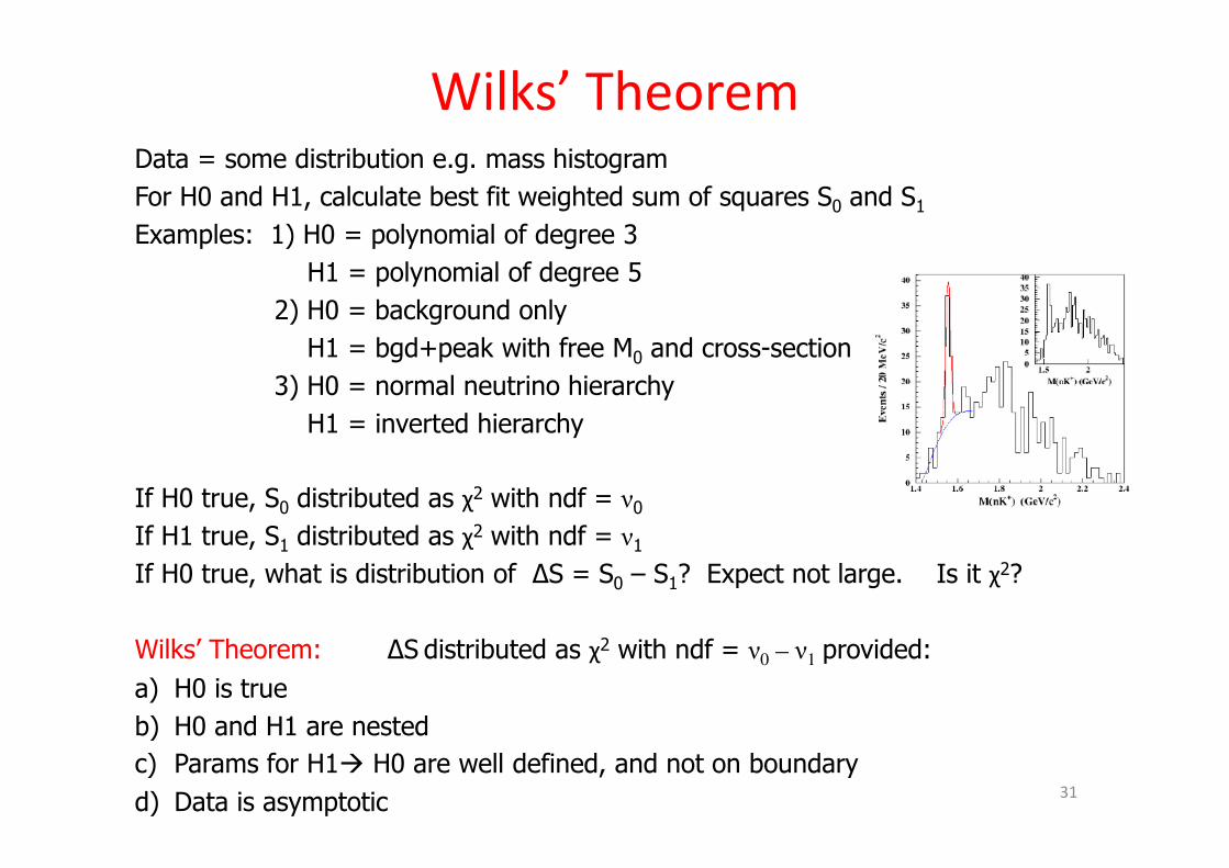
Wilks’ TheoremData = some distribution e.g. mass histogram
For H0 and H1, calculate best fit weighted sum of squares S0 and S1Examples: 1) H0 = polynomial of degree 3
H1 = polynomial of degree 5
2) H0 = background only
H1 = bgd+peak with free M0 and cross-section
3) H0 = normal neutrino hierarchy
H1 = inverted hierarchy
If H0 true, S0 distributed as χ2 with ndf = ν0
If H1 true, S1 distributed as χ2 with ndf = ν1
If H0 true, what is distribution of ∆S = S0 – S1? Expect not large. Is it χ2?
Wilks’ Theorem: ∆S distributed as χ2 with ndf = ν0 – ν1 provided:
a) H0 is true
b) H0 and H1 are nested
c) Params for H1� H0 are well defined, and not on boundary
d) Data is asymptotic 31
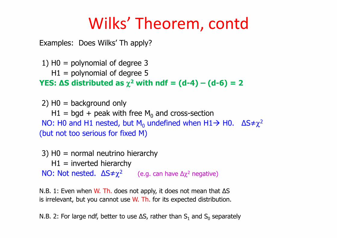
Wilks’ Theorem, contdExamples: Does Wilks’ Th apply?
1) H0 = polynomial of degree 3
H1 = polynomial of degree 5
YES: ∆S distributed as χχχχ2 with ndf = (d-4) – (d-6) = 2
2) H0 = background only
H1 = bgd + peak with free M0 and cross-section
NO: H0 and H1 nested, but M0 undefined when H1� H0. ∆S≠χ2
(but not too serious for fixed M)
3) H0 = normal neutrino hierarchy
H1 = inverted hierarchy
NO: Not nested. ∆S≠χ2 (e.g. can have ∆χ2 negative)
N.B. 1: Even when W. Th. does not apply, it does not mean that ∆S
is irrelevant, but you cannot use W. Th. for its expected distribution.
N.B. 2: For large ndf, better to use ∆S, rather than S1 and S0 separately
33
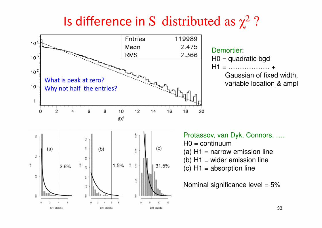
Is difference in S distributed as χ2 ?
Demortier:H0 = quadratic bgdH1 = ……………… +
Gaussian of fixed width,variable location & ampl
Protassov, van Dyk, Connors, ….H0 = continuum(a) H1 = narrow emission line(b) H1 = wider emission line(c) H1 = absorption line
Nominal significance level = 5%
What is peak at zero?
Why not half the entries?
34
So need to determine the ∆S distribution by Monte Carlo
N.B.
1) For mass spectrum, determining ∆S for hypothesis H1
when data is generated according to H0 is not trivial,
because there will be lots of local minima
2) If we are interested in 5σ significance level, needs lots of
MC simulations (or intelligent MC generation)
3) Asymptotic formulae may be useful (see K. Cranmer, G. Cowan,
E. Gross and O. Vitells, 'Asymptotic formulae for likelihood-based tests of new
physics', http://link.springer.com/article/10.1140%2Fepjc%2Fs10052-011-
1554-0 )
Is difference in S distributed as χ2 ?, contd.
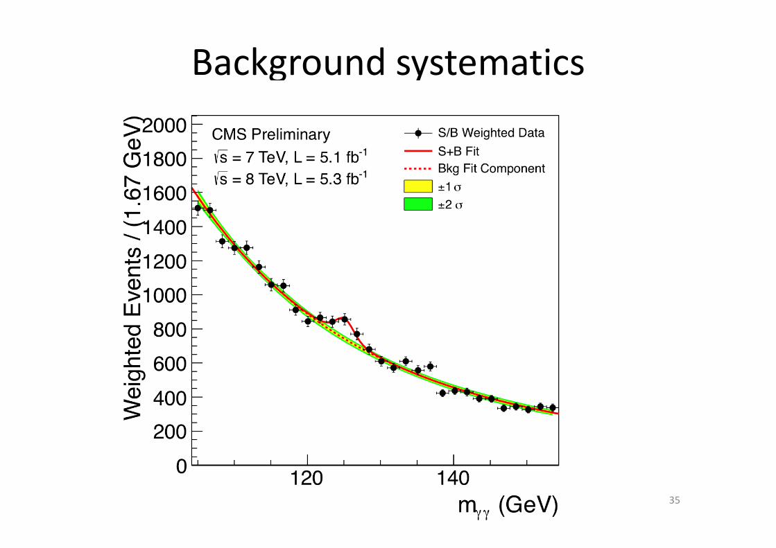
Background systematics
35
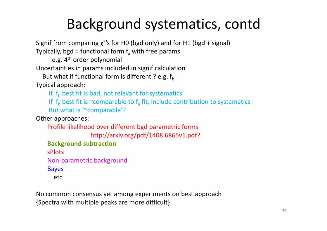
Background systematics, contdSignif from comparing χ2’s for H0 (bgd only) and for H1 (bgd + signal)
Typically, bgd = functional form fa with free params
e.g. 4th order polynomial
Uncertainties in params included in signif calculation
But what if functional form is different ? e.g. fb
Typical approach:
If fb best fit is bad, not relevant for systematics
If fb best fit is ~comparable to fa fit, include contribution to systematics
But what is ‘~comparable’?
Other approaches:
Profile likelihood over different bgd parametric forms
http://arxiv.org/pdf/1408.6865v1.pdf?
Background subtraction
sPlots
Non-parametric background
Bayes
etc
No common consensus yet among experiments on best approach
{Spectra with multiple peaks are more difficult}36
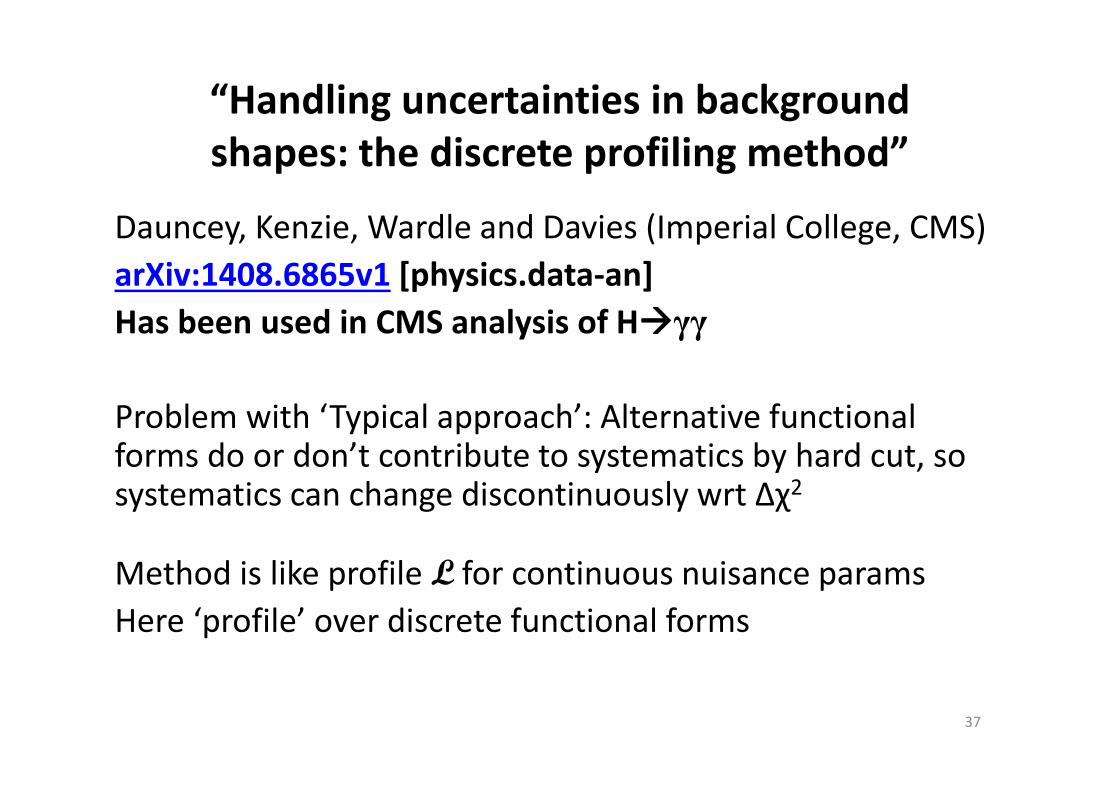
“Handling uncertainties in background
shapes: the discrete profiling method”
Dauncey, Kenzie, Wardle and Davies (Imperial College, CMS)
arXiv:1408.6865v1 [physics.data-an]
Has been used in CMS analysis of H����γγ
Problem with ‘Typical approach’: Alternative functional forms do or don’t contribute to systematics by hard cut, so systematics can change discontinuously wrt ∆χ2
Method is like profile L for continuous nuisance params
Here ‘profile’ over discrete functional forms
37
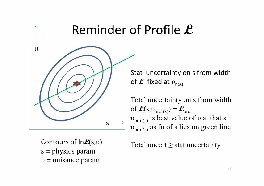
Reminder of Profile L
38
Contours of lnL(s,υ)s = physics param
υ = nuisance param
υ
s
Stat uncertainty on s from width
of L fixed at υbest
Total uncertainty on s from width
of L(s,υprof(s)) = Lprof
υprof(s) is best value of υ at that s
υprof(s) as fn of s lies on green line
Total uncert ≥ stat uncertainty

39
s
-2lnL
∆
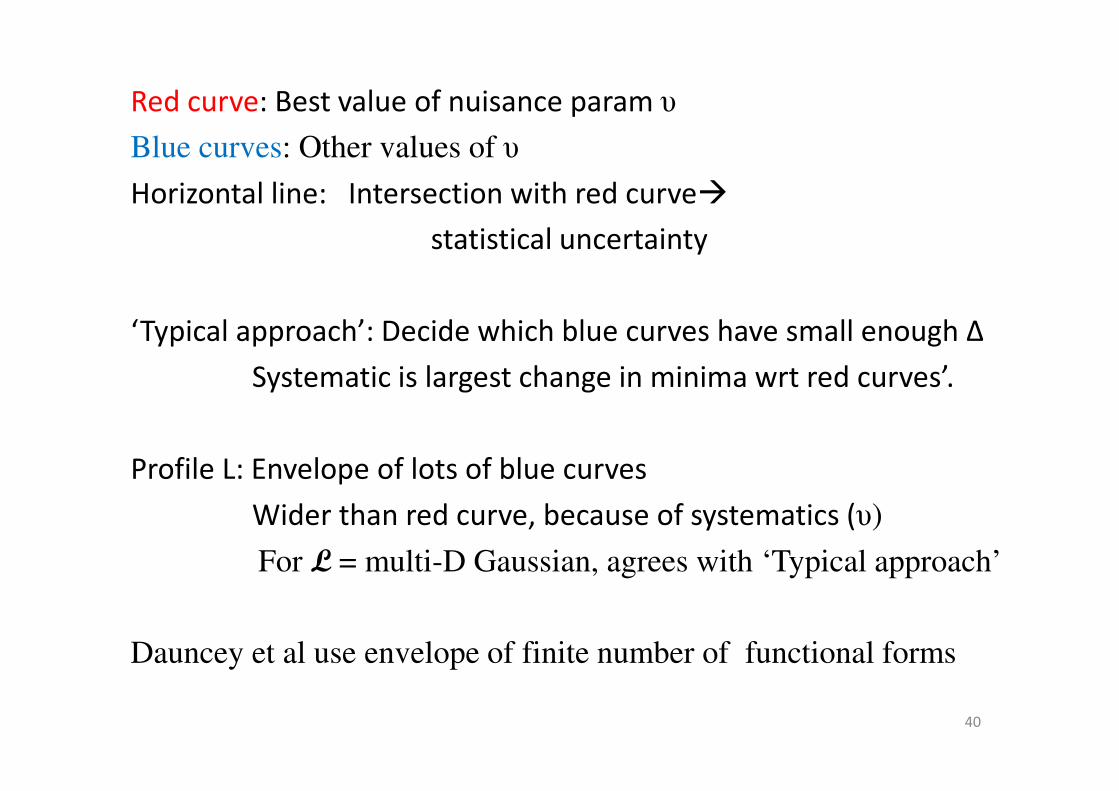
Red curve: Best value of nuisance param υ
Blue curves: Other values of υ
Horizontal line: Intersection with red curve�
statistical uncertainty
‘Typical approach’: Decide which blue curves have small enough ∆
Systematic is largest change in minima wrt red curves’.
Profile L: Envelope of lots of blue curves
Wider than red curve, because of systematics (υ)
For L = multi-D Gaussian, agrees with ‘Typical approach’
Dauncey et al use envelope of finite number of functional forms
40
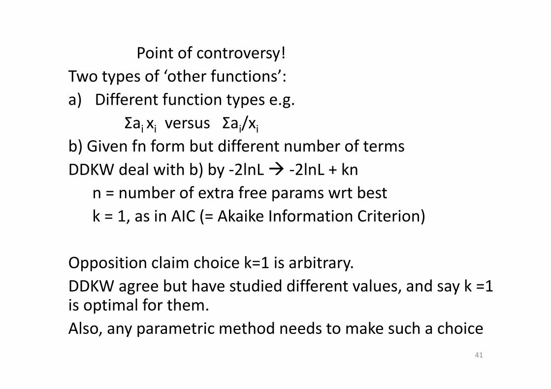
Point of controversy!
Two types of ‘other functions’:
a) Different function types e.g.
Σai xi versus Σai/xi
b) Given fn form but different number of terms
DDKW deal with b) by -2lnL � -2lnL + kn
n = number of extra free params wrt best
k = 1, as in AIC (= Akaike Information Criterion)
Opposition claim choice k=1 is arbitrary.
DDKW agree but have studied different values, and say k =1 is optimal for them.
Also, any parametric method needs to make such a choice
41
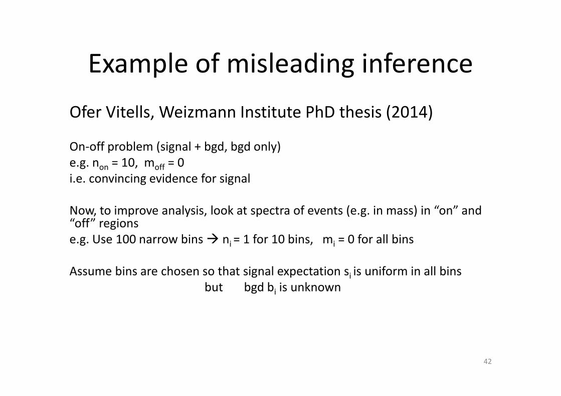
Example of misleading inference
Ofer Vitells, Weizmann Institute PhD thesis (2014)
On-off problem (signal + bgd, bgd only)
e.g. non = 10, moff = 0
i.e. convincing evidence for signal
Now, to improve analysis, look at spectra of events (e.g. in mass) in “on” and “off” regions
e.g. Use 100 narrow bins � ni = 1 for 10 bins, mi = 0 for all bins
Assume bins are chosen so that signal expectation si is uniform in all bins
but bgd bi is unknown
42
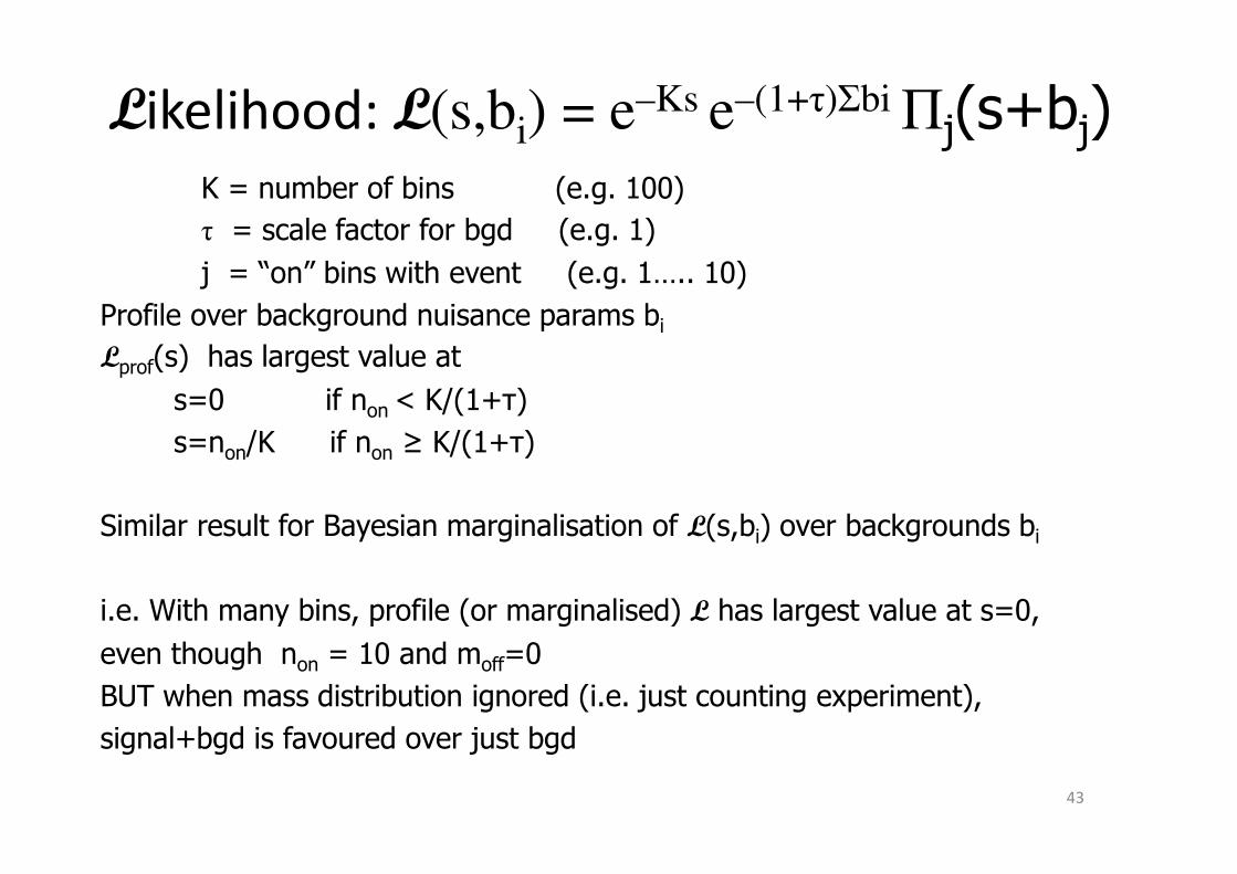
Likelihood: L(s,bi) = e–Ks e–(1+τ)Σbi Πj(s+bj)K = number of bins (e.g. 100)
τ = scale factor for bgd (e.g. 1)
j = “on” bins with event (e.g. 1….. 10)
Profile over background nuisance params biLprof(s) has largest value at
s=0 if non < K/(1+τ)
s=non/K if non ≥ K/(1+τ)
Similar result for Bayesian marginalisation of L(s,bi) over backgrounds bi
i.e. With many bins, profile (or marginalised) L has largest value at s=0,
even though non = 10 and moff=0
BUT when mass distribution ignored (i.e. just counting experiment),
signal+bgd is favoured over just bgd
43
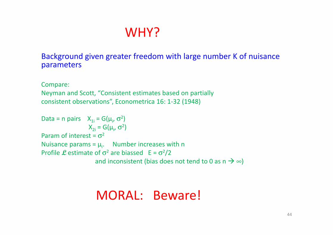
WHY?
Background given greater freedom with large number K of nuisance parameters
Compare:
Neyman and Scott, “Consistent estimates based on partially
consistent observations”, Econometrica 16: 1-32 (1948)
Data = n pairs X1i = G(µi, σ2)
X2i = G(µi, σ2)
Param of interest = σ2
Nuisance params = µi. Number increases with n
Profile L estimate of σ2 are biassed E = σ2/2
and inconsistent (bias does not tend to 0 as n � ∞)
MORAL: Beware!
44
45
WHY LIMITS?
Michelson-Morley experiment � death of aether
HEP experiments: If UL on expected rate for new
particle < expected, exclude particle
CERN CLW (Jan 2000)
FNAL CLW (March 2000)
Heinrich, PHYSTAT-LHC, “Review of Banff Challenge”
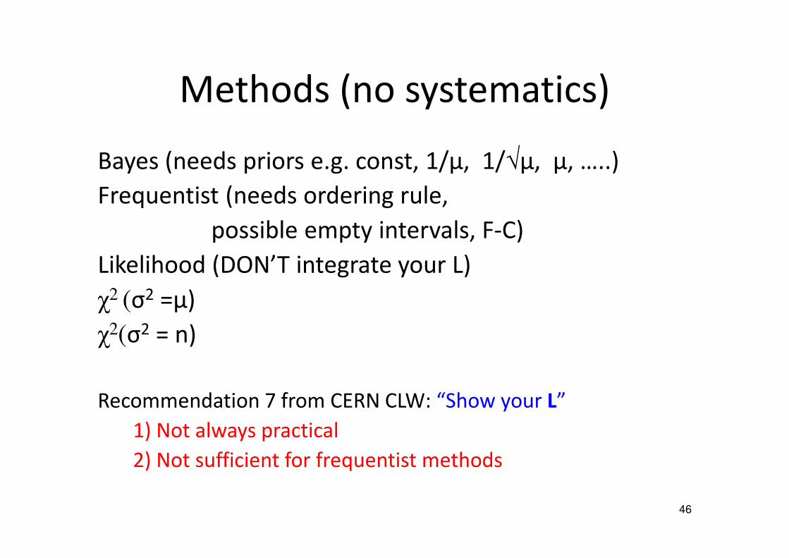
46
Bayes (needs priors e.g. const, 1/μ, 1/√μ, μ, …..)
Frequentist (needs ordering rule,
possible empty intervals, F-C)
Likelihood (DON’T integrate your L)
χ2 (σ2 =μ)
χ2(σ2 = n)
Recommendation 7 from CERN CLW: “Show your L”
1) Not always practical
2) Not sufficient for frequentist methods
Methods (no systematics)
47
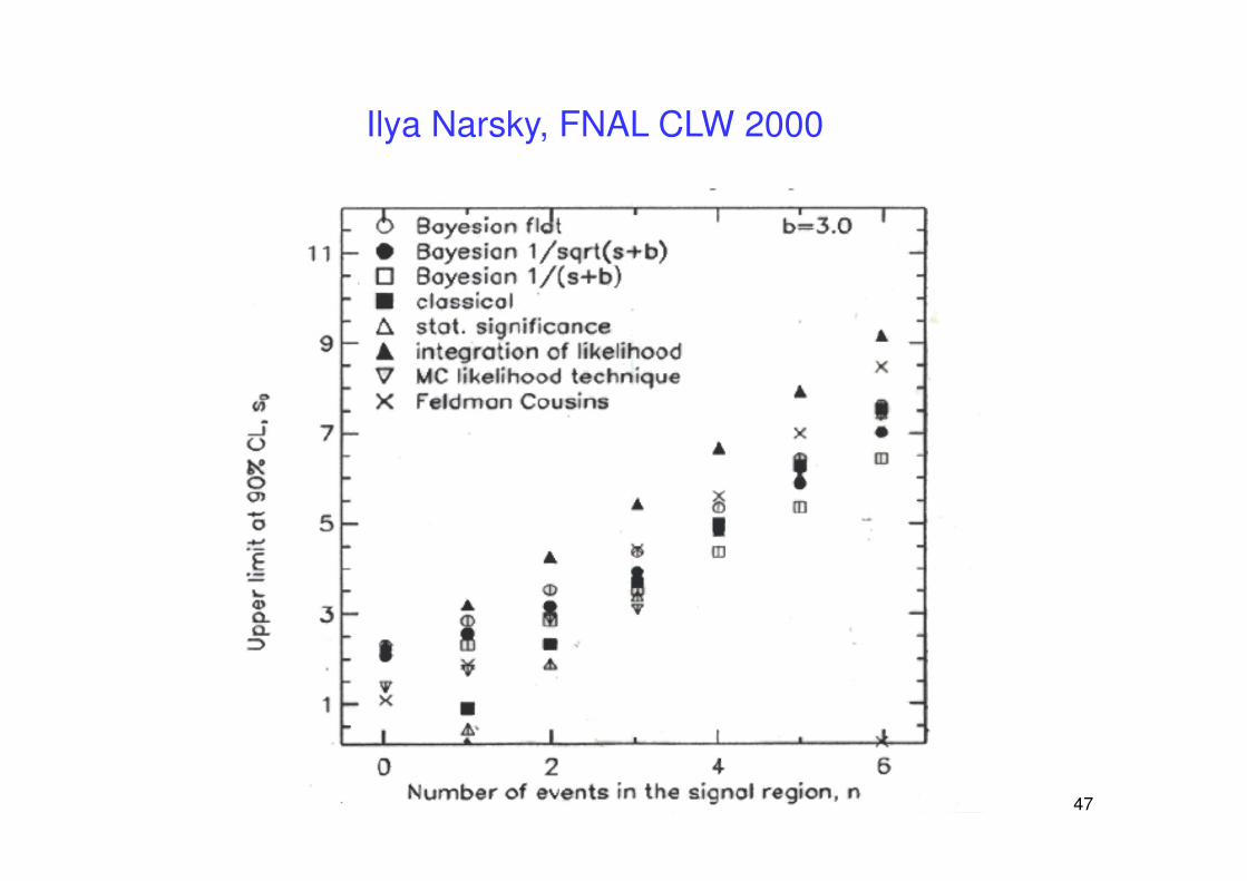
Ilya Narsky, FNAL CLW 2000
48
DESIRABLE PROPERTIES
• Coverage
• Interval length
• Behaviour when n < b
• Limit increases as σb increases
• Unified with discovery and interval estimation
49
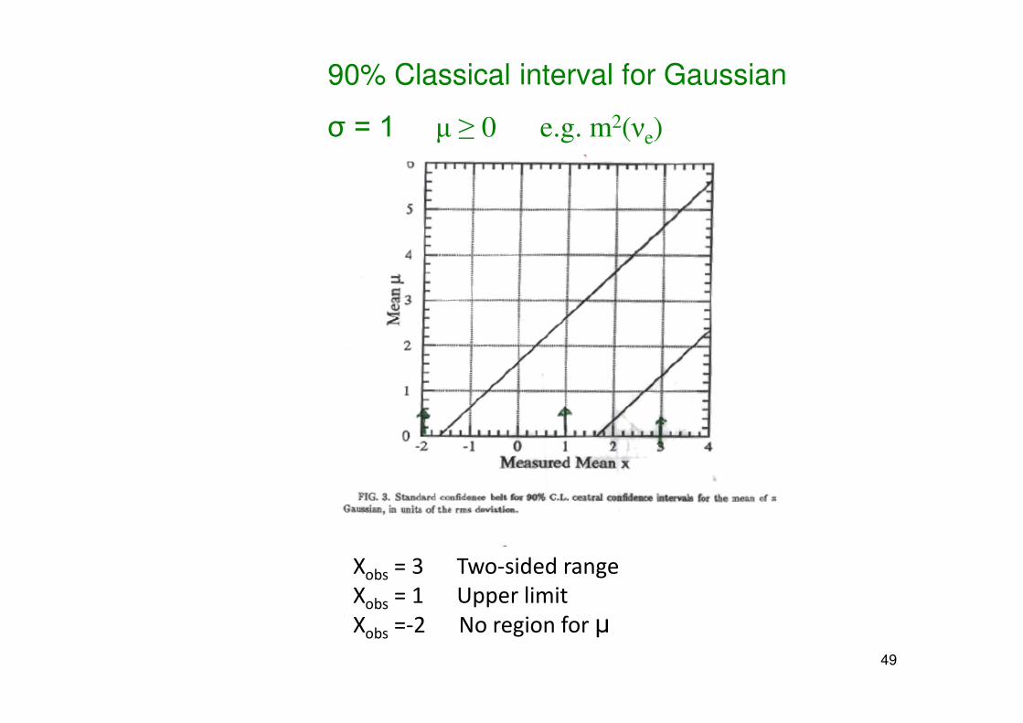
90% Classical interval for Gaussian
σ = 1 µ ≥ 0 e.g. m2(νe)
Xobs = 3 Two-sided range
Xobs = 1 Upper limit
Xobs =-2 No region for µ
50
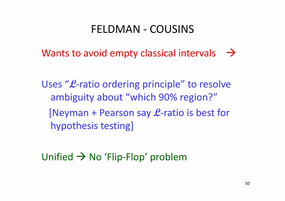
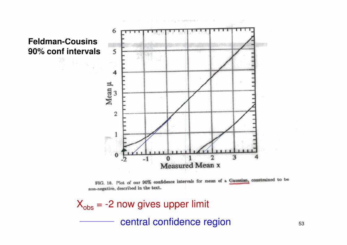
FELDMAN - COUSINS
Wants to avoid empty classical intervals �
Uses “L-ratio ordering principle” to resolve
ambiguity about “which 90% region?”
[Neyman + Pearson say L-ratio is best for
hypothesis testing]
Unified � No ‘Flip-Flop’ problem
51µ≥0 No prior for µ
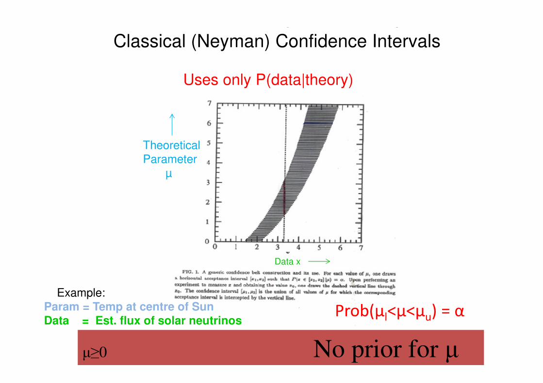
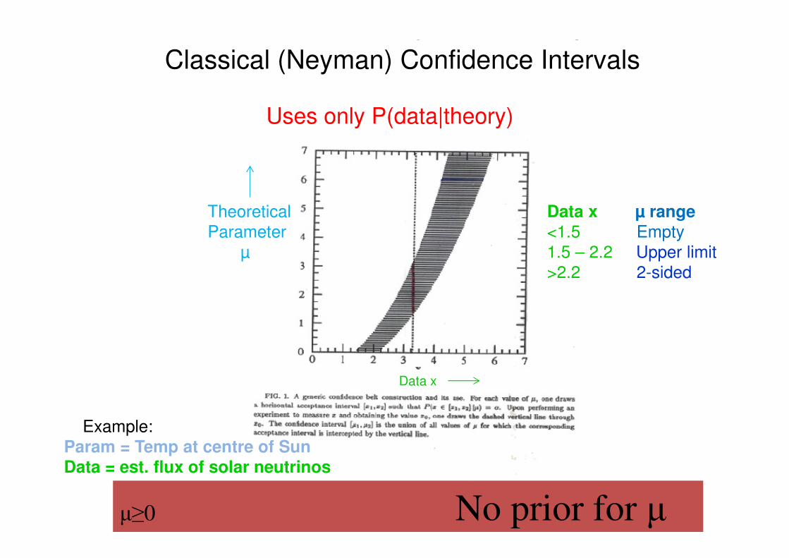
Classical (Neyman) Confidence Intervals
Uses only P(data|theory)
Example:Param = Temp at centre of SunData = Est. flux of solar neutrinos
Theoretical Parameter
µ
Data x
Prob(µl<µ<µu) = α
52µ≥0 No prior for µ
Classical (Neyman) Confidence Intervals
Uses only P(data|theory)
Example:Param = Temp at centre of SunData = est. flux of solar neutrinos
Theoretical Parameter
µ
Data x
Data x µ range<1.5 Empty1.5 – 2.2 Upper limit>2.2 2-sided
53
Xobs = -2 now gives upper limit
central confidence region
Feldman-Cousins 90% conf intervals
54
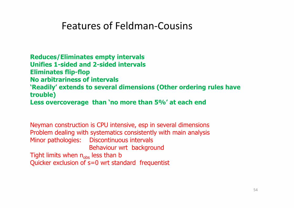
Features of Feldman-Cousins
Reduces/Eliminates empty intervalsUnifies 1-sided and 2-sided intervalsEliminates flip-flopNo arbitrariness of intervals‘Readily’ extends to several dimensions (Other ordering rules have trouble)Less overcoverage than ‘no more than 5%’ at each end
Neyman construction is CPU intensive, esp in several dimensionsProblem dealing with systematics consistently with main analysisMinor pathologies: Discontinuous intervals
Behaviour wrt backgroundTight limits when nobs less than bQuicker exclusion of s=0 wrt standard frequentist
55
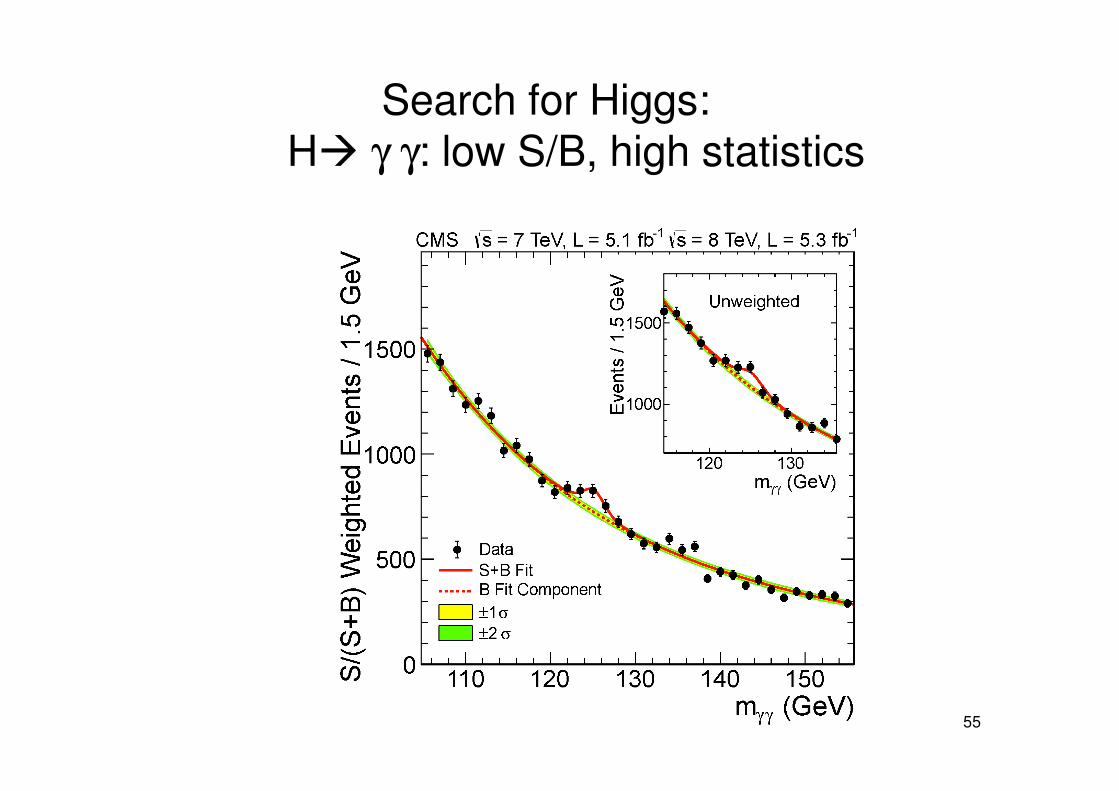
Search for Higgs:
H� γ γ: low S/B, high statistics
56
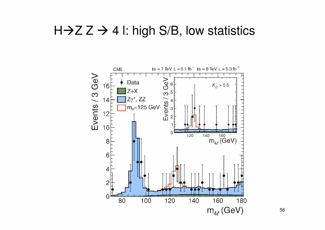
H�Z Z � 4 l: high S/B, low statistics
57
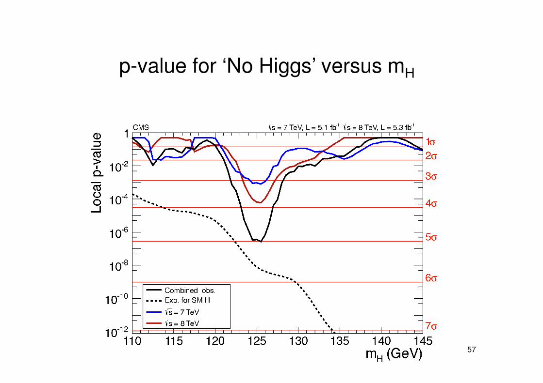
p-value for ‘No Higgs’ versus mH
58
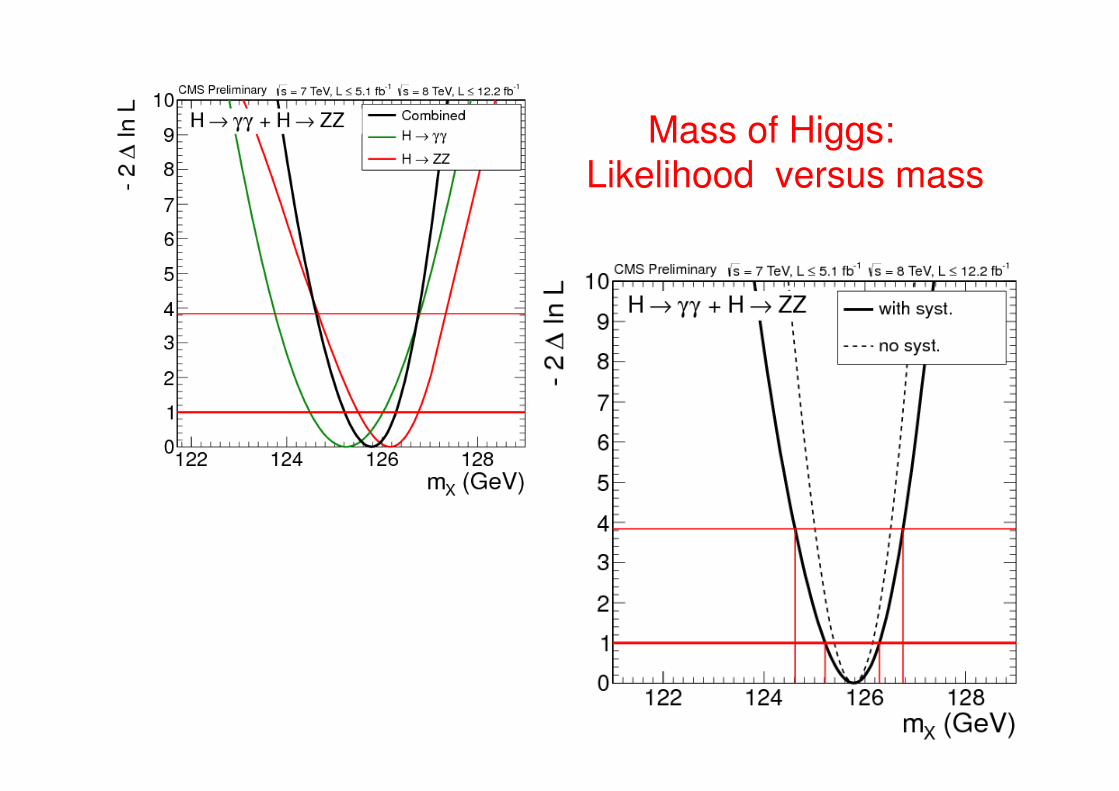
Mass of Higgs:
Likelihood versus mass
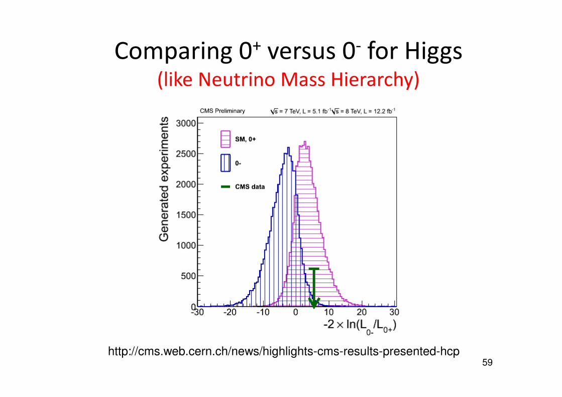
Comparing 0+ versus 0- for Higgs(like Neutrino Mass Hierarchy)
59http://cms.web.cern.ch/news/highlights-cms-results-presented-hcp
Conclusions
Resources:
Software exists: e.g. RooStats
Books exist: Barlow, Cowan, James, Lista, Lyons, Roe,…..
New: `Data Analysis in HEP: A Practical Guide to
Statistical Methods’ , Behnke et al.
PDG sections on Prob, Statistics, Monte Carlo
CMS and ATLAS have Statistics Committees (and BaBar and CDF earlier) – see their websites
Before re-inventing the wheel, try to see if Statisticians have already found a solution to your statistics analysis problem.
Don’t use a square wheel if a circular one already exists.
“Good luck” 60