IGS Tropospheric Products - Quality Verification and Assessment of Usefulness in Climatology

Michał Kruczyk , Tomasz Liwosz Warsaw University of Technology, Department of Geodesy and Geodetic Astronomy, Poland

Abstract Poster concentrates around two main questions. First is conformity study of ZTD of IPW in IGS tropospheric products (combination till 2006, final and ultra-rapid solutions by JPL, USNO, CODE), EPN tropospheric combination and me-teorological water vapour data sources. Water vapour data come from radiosoundings, global numerical weather prediction model GFS (operated by NCEP) and sun photometer CIMEL 318. Next topic is information potential contained in IGS tropospheric products for climatology and aerology. Long time series of IPW (daily averaged) can serve as climate change indicator e.g.: relatively unique shape of such series in different climates. Long lasting changes in weather conditions - ‘dry’ and ‘wet’ years are also visible. The longer and more homogenous our series the better chance to estimate the magnitude of climatological IWV changes. The problems with GPS stra-tegy and reference system changes can be solved by reprocessing (examples included). Next we adjust seasonal model to the series (LS method) for selected IGS stations. We apply two mo-des: sinusoidal and composite. Also two ways are tried: multi-year adjustment and every year separately (different are not only amplitudes but also phases). Even simple sinusoidal seasonal model of daily IPW values series clearly represents diversity of world climates. Residuals in periods up to 14 years are searched for some long-term IPW trend. For some stations & years such trends are quite clear, the following years not visible. IPW from IGS tropospheric products can be treated also as information source for aerology: it demonstrates some clear physical effects evoked by station location (e.g. height and series cor-relation coefficient as a function of distance) and weather patterns like dominant wind directions. Also deficiency of surface humidity data to model IPW is presented for different climates.

Introduction We can find several tropospheric solutions as part of the IGS poducts available in Data Centers repositories. These are: IGS combined product (till mid 2006, by G. Gend), IGS rapid combination (G. Gend), new IGS tropospheric product (from 2002 by Sung.H.Byun & Yoaz.E.Bar-Sever, JPL [1]), EUR - EPN combined product (by W. Soehne), IGS Analysis Centes in-dividual solutions: CODE, SIO, NGS, JPL, EMR and EPN Analysis Centes solutions. First we try to give some clues about quality of this solutions. Beyond simple statistical comprisons od ZTDs we use also some meteorological data - in the form of IPW. IPW (Integrated Precipitable Water) sometimes defined simply as PW is interesting meteorological parameter describing quantity of water vapour in the vertical direction over station in mm of liquid water after condensation. Related parameter IWV (Integrated Water Vapour) is also used which has the same numerical value but another unit of measure: kg/m2. IPW can be cal-culated from ZTD by known procedure of separtating ZHD (Zenith Hydrostatic Delay) and recalculating obtained ZWD (Zenith Wet Delay) by numerical coefficient dependent on so called ‘mean temperature’ in vertical profile of atmosphere. On the other hand we can get IPW from veritcal humidity data: integrating water vapour density (from radiosounding data but also from numerical weather prediction models). We have also some other techniques for IPW detection: WV radiometers and sun photometer. But the points equipped with them are quite sparse. From numerical weather predicton models we get IPW and ZTD for every station inside model grid.

Conclusions

1. IGS ZTDs show very good conformity in relation to EPN products from 2007 onwards. 2. Meteorological IPW (radiosoundings and sunphotometer) fits to IGS solutions, correlation diminishes quickly with distance. CIMEL sunphotometer data is most genuine source of IPW, as shows in situ

observation campaign. 3. Long series of IPW can be useful for climatology. Unfortunately there are too little homogenous solutions spanning many years. IPW trend depends on solution minutes. 4. There are many inconsistencies and errors in meteo Rinex files on IGS/EPN servers. Most difficult part of this work was cleaning of meteo data. References

[1] Sung H. Byun, Yoaz E. Bar-Sever: A new type of troposphere zenith path delay product of the international GNSS service. J Geod (2009) 83:367–373

Acknowledgements

• Polish Ministry of Science and Higher Education (National Science Center) – grant Nr N N526 074038 • IGS/EPN products developers • Marcin Rajner (Warsaw University of Technology) - maps in GMT • Aleksander Piotruczuk - Institute of Geophysics, Polish Academy of Sciences – BELS station maintenance and other help • National Centers for Environmental Prediction (NCEP) - GFS model data • University of Wyoming – radiosounding data • NASA, AERONET (Brent Holben) – sunphotometer data analysis lev15/20

Contact: kruczyk@gik.pw.edu.pl, t.liwosz@gik.pw.edu.pl

)(]/[][ ,02 ZHDZTDZWDdhmkgIWVmmIPW wtropv −⋅=⋅=Δ⋅≈== ∫ κκκρ

Now You can compare this conformity with excellent results for other technique collocation for the same year 2010. This is sunphotometer. Polish Academy of Sciences operates CIMEL CF-318 sunphotometer at Central Geophysical Observatory in Belsk near Warsaw (λ = 20°47’30”, φ = 51°50’12”, h = 190.0 m), 33 km from JOZE in the frame of AERONET (AErosol RObotic NETwork) network coordinated by NASA & CNRS. There has been set up periodical GPS point BELS at the roof of the building of Central Geophysical Observatory Institute of Geophysics PAS in Belsk. Trimble 4000 SSE receiver has been permanently instal-led by our Department of Geodesy and Geodetic Astronomy (till May 2009 JOZE station receiver - one of the oldest in the whole network) and works permanently thereafter from July 2009. Decrease of correlation characteristic for COSMO-LM model comparisons with GNSS and GNSS vs. in situ technique is attained for Belsk-BOGI pair: distance 73 km!

IGS Workshop 2012 Olsztyn, 23--27 July 2012

BELS 2010

0

5

10

15

20

25

30

35

40

45

0 5 10 15 20 25 30 35 40 45

IPW [mm] CIMEL sunphotometer, Belsk

IPW

[mm

] GPS

, Bel

sk

Belsk CIMEL – Belsk GPS correlation coefficient: 0.997 Belsk CIMEL - JOZ2 GPS (IGS): 0.988 Belsk CIMEL – BOGI GPS(EUR) : 0.979

Fig. 5 Belsk IPW: CIMEL-318 measurements and GPS BELS (WUT dedicated solution), JOZ2 (IGS solution) and BOGI (EPN combnation) in 2010

ZTD conformity analysis Tropospheric combination provided us with easy mean to asses solution discrepancies for each station. Look for instance at weekly differences for REYK.

Fig. 6 IPW maps for 25 and 27 June 2011 12:00 UT from GFS global model (note: we need 2 day time step to see discernible change in global IPW pattern

JOZ2 2010 IGS new

0

5

10

15

20

25

30

35

40

45

0 5 10 15 20 25 30 35 40 45

IPW [mm] CIMEL sunphotometer, Belsk

IPW

[mm

] GPS

, JO

ZE

NWP model GFS as a source of IPW As meteorological database to calculate ZTD and IPW we tested input fields (after assimilation) of GFS (Global Forecast System) model maintained by National Centers for Environmental Prediction (NCEP), grids after analysis are available 4 time a day (UT 00 06 12 18) in 0.5° resolution grid (720x181 nodes). We can use also first prognosis step (T+3h) to get 3-hour time resolution. Comparison have ben made of IPW series from GFS model input fields and first prognosis steps with IGS final solution (USNO and JPL [1]). Direct comparison is possible only for sites equipped with meteorological sensors. But treating NWP input fields (after assimilation) as meteorological database we can calculate IPW for every station inside grid.

Meteorological data for IPW verification Most popular meteorological data to calculate IPW are free flying balloon radiosoundings (RAOBs) carried out 2 - 4 time a day in some points close to GNSS station. All comparisons from now are made in values of IPW.

radiosounding point GPS solution distance [km] RAOB point height [m] bias [mm] mean absolute

bias [mm]difference

std dev [mm]difference RMS [mm]

no of points

6610 SW PAYERNE ZIMM 14001M004 cod 43.84 491 2.93 2.97 1.69 3.38 66711520 CZ PRAHA-LIBUS GOPE 11502M002 cod 29.21 303 2.31 2.38 1.68 2.86 113712374 PL LEGIONOWO BOGO 12207M002 cod 12.47 96 1.11 1.64 1.9 2.2 25912374 PL LEGIONOWO JOZ2 12204M002 cod 34.79 96 1.2 1.6 1.64 2.03 71812374 PL LEGIONOWO JOZE 12204M001 cod 34.83 96 0.35 1.21 1.67 1.71 71310393 DL LINDENBERG POTS 14106M003 cod 73.09 115 1.07 1.57 1.75 2.05 30610771 DL KUEMMERSRUCK WTZR 14201M010 cod 76.5 418 1.31 1.72 1.78 2.21 1369

3238 UK Albemarle MORP 13299S001 igs (n) 26.44 141 -0.45 1.2 1.66 1.72 32111520 CZ PRAHA-LIBUS GOPE 11502M002 igs (n) 29.21 303 2.27 2.32 1.52 2.73 123812374 PL LEGIONOWO JOZ2 12204M002 igs (n) 34.79 96 1.35 1.66 1.53 2.04 72012374 PL LEGIONOWO JOZE 12204M001 igs (n) 34.83 96 0.41 1.29 1.76 1.81 73012425 PL WROCLAW I WROC 12217M001 igs (n) 18.35 122 0.37 1.12 2.53 2.56 68417062 TU ISTANBUL/GOZTE ISTA 20807M001 igs (n) 22.79 33 1.54 1.83 1.79 2.36 65510393 DL LINDENBERG POTS 14106M003 igs (n) 73.09 115 1.28 1.62 1.62 2.07 31210771 DL KUEMMERSRUCK WTZR 14201M010 igs (n) 76.5 418 1.49 1.61 1.08 1.84 417

6610 SW PAYERNE ZIMM 14001M004 ngs 43.84 491 3.13 3.16 1.75 3.59 49811520 CZ PRAHA-LIBUS GOPE 11502M002 ngs 29.21 303 2.09 2.14 1.38 2.5 49412374 PL LEGIONOWO JOZE 12204M001 ngs 34.83 96 0.69 1.27 1.57 1.71 530

-8

-6

-4

-2

0

2

4

6

8

1000 1050 1100 1150 1200 1250 1300 1350 1400

GPS week

delta

ZTD

[mm

]

CODESAGFZJPLNOANRCSIOEUR

year ACs solutions mean difference [mm]

mean absolute difference

difference STDEV

difference RMS No. stations

2004 EUR-SIO 5.68 6.30 4.79 7.52 332005 EUR-SIO 1.91 8.47 13.80 14.37 282005 EUR-IGS(n) 6.47 7.06 4.75 8.22 242007 EUR-IGS(r) -0.55 2.32 3.13 3.25 292007 IGS(n)-IGS(r) 0.15 3.20 4.24 4.45 442007 EUR-IGS(n) 0.09 2.61 3.38 3.64 302009 EUR-EMR -0.32 2.52 2.95 3.24 102009 NGS-EMR 0.55 3.93 4.37 5.02 572009 EUR-JPL -0.79 2.59 4.53 4.89 132009 EUR-NGS -0.27 2.50 3.17 3.33 452009 NGS-IGS(n) -0.06 3.16 3.97 4.22 502010 EUR-JPL -0.16 2.73 5.82 6.06 142010 EUR-NGS -0.29 2.14 2.79 2.97 452010 NGS-IGS(n) -0.22 3.00 4.33 4.58 462010 COD-IGS(n) 0.21 2.86 4.24 4.44 632011 EUR-JPL -0.50 2.66 5.55 5.79 162011 EUR-NGS -0.21 2.12 2.66 2.87 442011 NGS-IGS(n) -0.09 3.17 6.08 6.29 542011 COD-IGS(n) -0.11 3.16 6.36 6.50 59

0

2

4

6

8

10

12

14

0 10 20 30 40 50 60 70 80 90

latitude [deg]

ZTD

diff

eren

ce R

MS

[mm

]

Fig. 1 Weekly ZTD biases of IGS Centers tropospheric solutions in relation to IGS tropospheric combination Fig. 2 Average ZTD difference RMS in 2010: CODE vs. new IGS tropospheric

product in relation to station latitude

Tab. 1 Statistics of ZTD solutions: IGS(n) - new IGS tropospheric product, IGS(r) - rapis troposheric combination

Fig. 3 ZTD differences for 2 stations:EPN tropospheric combination - IGS tropospheric product in 2010

-30

-20

-10

0

10

20

30

0 50 100 150 200 250 300 350

DOY 2010

delta

ZTD

[mm

]

LAMASASS

Tab. 2 Comparison of selected radiosoundings and nearby GPS stations (three IGS tropo solutions) in 2011

Fig. 4 IPW [mm] 2011 from radiosounding and GPS for 3 stations pairs with increasing distance: RAOB Wrocław - WROC (IGS (n)) - 18 km, RAOB Legionowo – JOZE (COD) - 35 km, RAOB Kuemmersruck – WTZR (COD) - 77 km.

0

5

10

15

20

25

30

35

40

0 5 10 15 20 25 30 35 40

radiosounding Wroclaw I

GP

S W

RO

C - I

GS

new

0

5

10

15

20

25

30

35

40

0 5 10 15 20 25 30 35 40

radiosounding Legionowo

GP

S J

OZE

- C

OD

0

5

10

15

20

25

30

35

40

0 5 10 15 20 25 30 35 40

radiosounding Kuemersruck

GPS

WTZ

R -

COD

BOGI 2010 EUR

0

5

10

15

20

25

30

35

40

45

0 5 10 15 20 25 30 35 40 45

IPW [mm] CIMEL sunphotometer, Belsk

IPW

[mm

] GPS

, JO

ZE

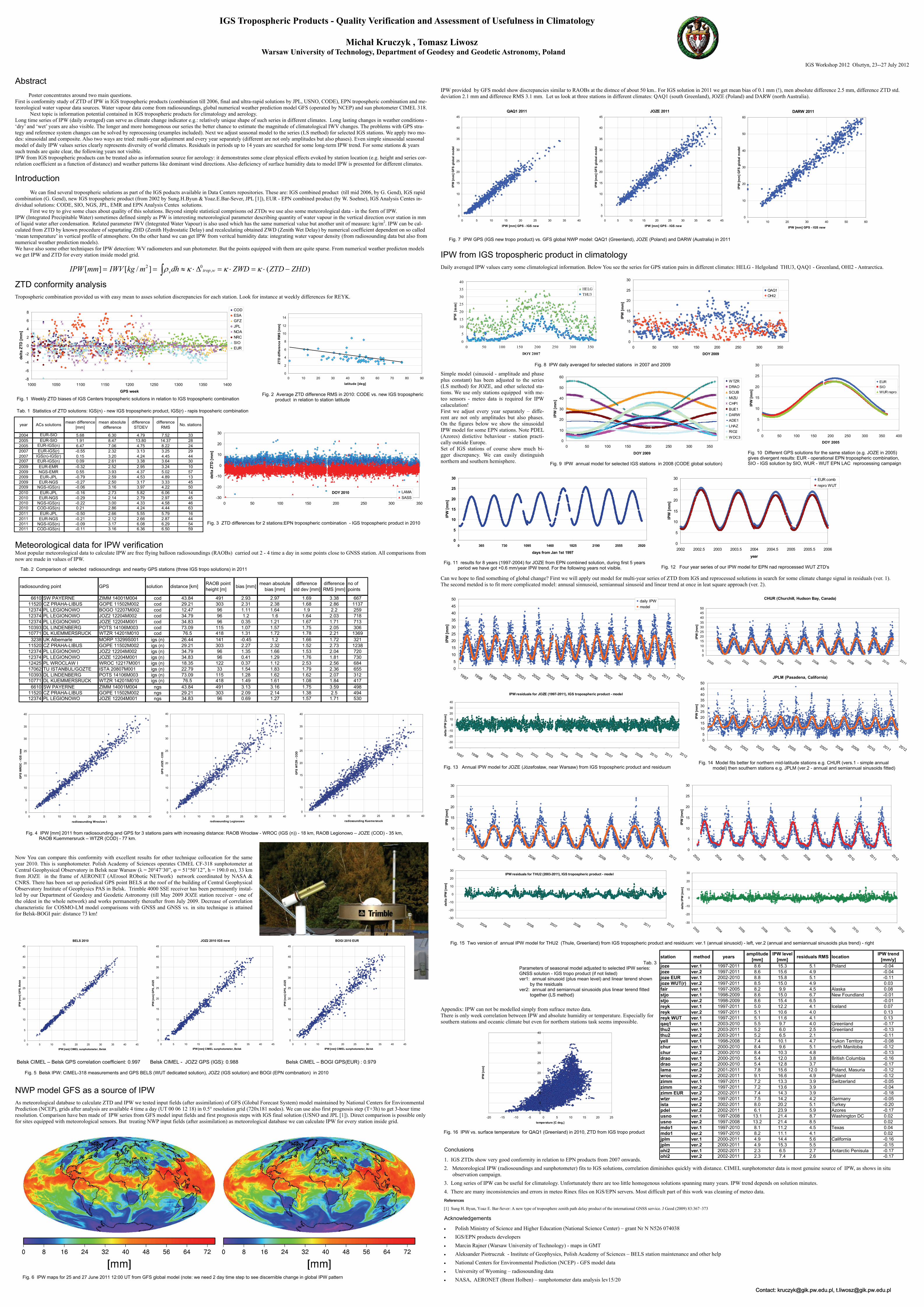
IPW provided by GFS model show discrepancies similar to RAOBs at the distnce of about 50 km.. For IGS solution in 2011 we get mean bias of 0.1 mm (!), men absolute difference 2.5 mm, difference ZTD std. deviation 2.1 mm and difference RMS 3.1 mm. Let us look at three stations in different climates: QAQ1 (south Greenland), JOZE (Poland) and DARW (north Australia).

QAQ1 2011

0

5

10

15

20

25

30

35

40

45

0 5 10 15 20 25 30 35 40

IPW [mm] GPS - IGS new

IPW

[mm

] GFS

glo

bal m

odel

JOZE 2011

0

5

10

15

20

25

30

35

40

45

0 5 10 15 20 25 30 35 40 45

IPW [mm] GPS - IGS new

IPW

[mm

] GFS

glo

bal m

odel

DARW 2011

0

10

20

30

40

50

60

0 10 20 30 40 50 60

IPW [mm] GPS - IGS new

IPW

[mm

] GFS

glo

bal m

odel

Fig. 7 IPW GPS (IGS new tropo product) vs. GFS global NWP model: QAQ1 (Greenland), JOZE (Poland) and DARW (Australia) in 2011

IPW from IGS tropospheric product in climatology Daily averaged IPW values carry some climatological information. Below You see the series for GPS station pairs in different climates: HELG - Helgoland THU3, QAQ1 - Greenland, OHI2 - Antrarctica.

0

5

10

15

20

25

30

35

40

0 50 100 150 200 250 300 350

DOY 2007

IPW

[mm

]

HELGTHU3

0

5

10

15

20

25

30

0 50 100 150 200 250 300 350

DOY 2009

IPW

[mm

]

QAQ1OHI2

0

10

20

30

40

50

60

0 50 100 150 200 250 300 350

DOY 2009

IPW

[mm

]

WTZRDRAOSCUBMIZUCHPIBUE1DARWADE1LHAZRIO2WDC3

0

5

10

15

20

25

30

0 50 100 150 200 250 300 350 400

DOY 2005

IPW

[mm

]

EURSIOWUR repro

0

5

10

15

20

25

30

0 365 730 1095 1460 1825 2190 2555 2920

days from Jan 1st 1997

IPW

[mm

]

0

5

10

15

20

25

30

2002 2002.5 2003 2003.5 2004 2004.5 2005 2005.5 2006

year

IPW

[mm

]

EUR combrepro WUT

0

5

10

15

20

25

30

20032004

20052006

20072008

20092010

20112012

IPW

[mm

]

IPW residuals for THU2 (2003-2011), IGS tropospheric product - model

-30

-20

-10

0

10

20

30

20032004

20052006

20072008

20092010

20112012

delta

IPW

[mm

]

Fig. 8 IPW daily averaged for selected stations in 2007 and 2009

Simple model (sinusoid - amplitude and phase plus constant) has been adjusted to the series (LS method) for JOZE, and other selected sta-tions. We use only stations equipped with me-teo sensors - meteo data is required for IPW calaculation! First we adjust every year separately – diffe-rent are not only amplitudes but also phases. On the figures below we show the sinusoidal IPW model for some EPN stations. Note PDEL (Azores) distictive behaviour - station practi-cally outside Europe. Set of IGS stations of course show much bi-gger discrepancy. We can easily distinguish northern and southern hemisphere. Fig. 9 IPW annual model for selected IGS stations in 2008 (CODE global solution)

Fig. 10 Different GPS solutions for the same station (e.g. JOZE in 2005) gives divergent results: EUR - operational EPN tropospheric combination, SIO - IGS solution by SIO, WUR - WUT EPN LAC reprocessing campaign

Fig. 12 Four year series of our IPW model for EPN nad reprocessed WUT ZTD's Fig. 11 results for 8 years (1997-2004) for JOZE from EPN combined solution, during first 5 years

period we have got +0.6 mm/year IPW trend. For the following years not visible.

Can we hope to find something of global change? First we will apply out model for multi-year series of ZTD from IGS and reprocessed solutions in search for some climate change signal in residuals (ver. 1). The second metdod is to fit more complicated model: annusal sinnusoid, semiannual sinusoid and linear trend at once in leat square approach (ver. 2).

0

5

10

15

20

25

30

35

40

45

50

19971998

19992000

20012002

20032004

20052006

20072008

20092010

20112012

IPW

[mm

]

daily IPWmodel

IPW residuals for JOZE (1997-2011), IGS tropospheric product - model

-40

-30

-20

-10

0

10

20

30

40

19971998

19992000

20012002

20032004

20052006

20072008

20092010

20112012

delta

IPW

[mm

]

0

5

10

15

20

25

30

20032004

20052006

20072008

20092010

20112012

IPW

[mm

]

-30

-20

-10

0

10

20

30

20032004

20052006

20072008

20092010

20112012

delta

IPW

[mm

]

CHUR (Churchill, Hudson Bay, Canada)

05

101520253035404550

20002001

20022003

20042005

20062007

20082009

20102011

IPW

[mm

]

JPLM (Pasadena, California)

05

101520253035404550

20002001

20022003

20042005

20062007

20082009

20102011

2012

IPW

[mm

]

Fig. 13 Annual IPW model for JOZE (Józefosław, near Warsaw) from IGS tropospheric product and residuum

Fig. 14 Model fits better for northern mid-latitude stations e.g. CHUR (vers.1 - simple annual model) then southern stations e.g. JPLM (ver.2 - annual and semiannual sinusoids fitted)

Fig. 15 Two version of annual IPW model for THU2 (Thule, Greenland) from IGS tropospheric product and residuum: ver.1 (annual sinusoid) - left, ver.2 (annual and semiannual sinusoids plus trend) - right

station method years amplitude [mm]

IPW level [mm] residuals RMS location IPW trend

[mm/y]joze ver.1 1997-2011 8.6 15.3 5.1 Poland -0.04joze ver.2 1997-2011 8.6 15.6 4.9 -0.04joze EUR ver.1 2002-2010 8.8 15.8 5.1 -0.11joze WUT(r) ver.2 1997-2011 8.5 15.0 4.9 0.03fair ver.1 1997-2005 8.2 9.9 4.5 Alaska 0.08stjo ver.1 1998-2009 8.6 15.0 6.7 New Foundland -0.01stjo ver.2 1998-2009 8.6 15.4 6.5 -0.01reyk ver.1 1997-2011 5.0 12.2 4.1 Iceland 0.07reyk ver.2 1997-2011 5.1 10.6 4.0 0.13reyk WUT ver.1 1997-2011 5.1 11.6 4.1 0.13qaq1 ver.1 2003-2010 5.5 9.7 4.0 Greenland -0.17thu2 ver.1 2003-2011 5.2 6.0 2.5 Greenland -0.13thu2 ver.2 2003-2011 5.2 6.5 2.1 -0.11yell ver.1 1998-2008 7.4 10.1 4.7 Yukon Territory -0.08chur ver.1 2000-2010 8.4 9.6 5.1 north Manitoba -0.12chur ver.2 2000-2010 8.4 10.3 4.8 -0.13drao ver.1 2000-2010 5.4 12.0 3.8 British Columbia -0.16drao ver.2 2000-2010 5.4 12.8 3.7 -0.17lama ver.2 2001-2011 7.8 15.6 12.0 Poland, Masuria -0.12wroc ver.2 2002-2011 9.1 16.6 4.9 Poland -0.12zimm ver.1 1997-2011 7.2 13.3 3.9 Switzerland -0.05zimm ver.2 1997-2011 7.2 13.6 3.9 -0.04zimm EUR ver.2 2002-2011 7.4 14.3 3.9 -0.18wtzr ver.2 1997-2011 7.5 14.2 4.2 Germany -0.05ista ver.2 2002-2011 8.0 20.2 5.1 Turkey -0.20pdel ver.2 2002-2011 6.1 23.9 5.9 Azores -0.17usno ver.1 1997-2008 13.1 21.4 8.7 Washington DC 0.02usno ver.2 1997-2008 13.2 21.4 8.5 0.02mdo1 ver.1 1997-2010 8.1 11.2 4.5 Texas 0.04mdo1 ver.2 1997-2010 8.2 11.1 4.1 0.02jplm ver.1 2000-2011 4.9 14.4 5.6 California -0.16jplm ver.2 2000-2011 4.9 15.3 5.5 -0.15ohi2 ver.1 2002-2011 2.3 6.5 2.7 Antarctic Penisula -0.17ohi2 ver.2 2002-2011 2.3 7.4 2.6 -0.17

Tab. 3 Parameters of seasonal model adjusted to selected IPW series: GNSS solution - IGS tropo product (if not listed) ver1: annual sinusoid (plus mean level) and linear terend shown

by the residuals ver2: annual and semiannual sinusoids plus linear terend fitted

together (LS method)

Appendix: IPW can not be modelled simply from sufrace meteo data. There is only week correlation between IPW and absolute humidity or temperature. Especially for southern stations and oceanic climate but even for northern stations task seems impossible.

0

5

10

15

20

25

30

35

40

-20 -15 -10 -5 0 5 10 15 20 25

temperature [C deg.]

IPW

[mm

]

Fig. 16 IPW vs. surface temperature for QAQ1 (Greenland) in 2010, ZTD from IGS tropo product