Iosif Salem - Εθνικόν και Καποδιστριακόν...

National and Kapodistrian University of Athens

Graduate Program in Logic, Algorithmsand Computation

MSc thesis

On the computability of obstruction sets forwell–quasi–ordered graph classes

Iosif Salem

supervised by:

Dimitrios M. Thilikos

September 17, 2012

To the memory of my father,Guido Salem

Η παρούσα Διπλωματική Εργασία

εκπονήθηκε στα πλαίσια των σπουδών

για την απόκτηση του

Μεταπτυχιακού Διπλώματος Ειδίκευσης

στη

Λογική και Θεωρία Αλγορίθμων και Υπολογισμού

που απονέμει το

Τμήμα Μαθηματικών

του

Εθνικού και Καποδιστριακού Πανεπιστημίου Αθηνών

Εγκρίθηκε την 17η Σεπτεμβρίου 2012 από Εξεταστική Επιτροπή

αποτελούμενη από τους:

Ονοματεπώνυμο Βαθμίδα Υπογραφή

1. : Δ. Θηλυκός Αναπλ. Καθηγητής ……………………

2. : Ε. Κυρούσης Καθηγητής ……………………

3. : Στ. Κολλιόπουλος Αναπλ. Καθηγητής ……………………

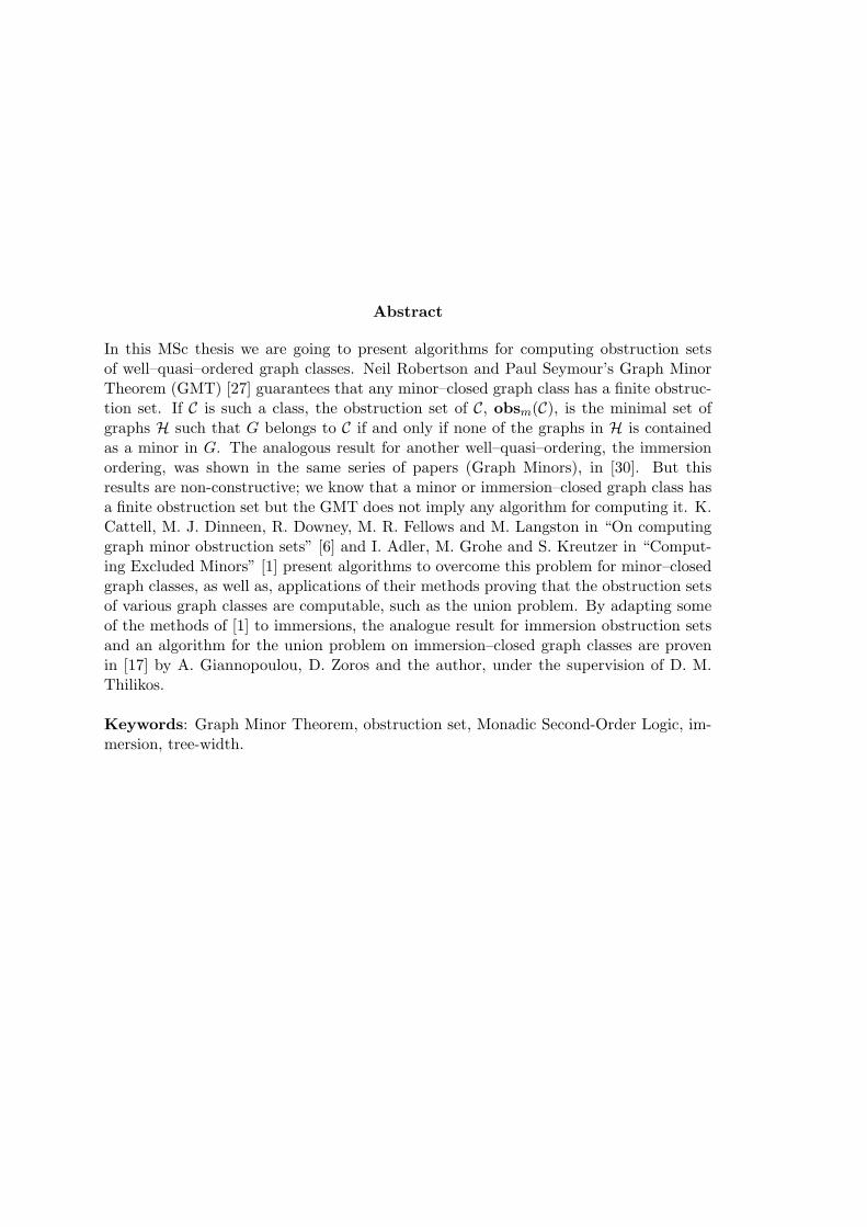
Abstract

In this MSc thesis we are going to present algorithms for computing obstruction setsof well–quasi–ordered graph classes. Neil Robertson and Paul Seymour’s Graph MinorTheorem (GMT) [27] guarantees that any minor–closed graph class has a finite obstruc-tion set. If C is such a class, the obstruction set of C, obsm(C), is the minimal set ofgraphs H such that G belongs to C if and only if none of the graphs in H is containedas a minor in G. The analogous result for another well–quasi–ordering, the immersionordering, was shown in the same series of papers (Graph Minors), in [30]. But thisresults are non-constructive; we know that a minor or immersion–closed graph class hasa finite obstruction set but the GMT does not imply any algorithm for computing it. K.Cattell, M. J. Dinneen, R. Downey, M. R. Fellows and M. Langston in “On computinggraph minor obstruction sets” [6] and I. Adler, M. Grohe and S. Kreutzer in “Comput-ing Excluded Minors” [1] present algorithms to overcome this problem for minor–closedgraph classes, as well as, applications of their methods proving that the obstruction setsof various graph classes are computable, such as the union problem. By adapting someof the methods of [1] to immersions, the analogue result for immersion obstruction setsand an algorithm for the union problem on immersion–closed graph classes are provenin [17] by A. Giannopoulou, D. Zoros and the author, under the supervision of D. M.Thilikos.

Keywords: Graph Minor Theorem, obstruction set, Monadic Second-Order Logic, im-mersion, tree-width.

Acknowledgements

This master thesis would not have been possible without the support of many people.I would like to thank my supervisor Dimitrios M. Thilikos for introducing me to a veryinteresting theory that combines Algorithmic Graph Theory and Mathematical Logic,and also for introducing me to Theoretical Computer Science through his lectures inTheory of Algorithms, Computational Complexity, Recursion Theory and Graph Theoryduring my undergraduate studies in the Department of Mathematics of the University ofAthens. In addition, I would like to thank Archontia Giannopoulou and Dimitris Zorosfor collaborating with me and for making this project even more interesting.

I would also like to thank the members of the supervisory committee Stavros Kol-liopoulos and Lefteris Kirousis, and all the professors of the graduate program in “Logic,Algorithms and Computation” (MPLA) for their stimulating lectures and for giving amodel of how a professor should be like. I should also thank the secretariats of MPLAfor being so helpfull, patient and efficient anytime needed.

Above all, I would like to thank my parents Guido and Sarra and my sister Louizafor all their support and love, and for many things that words cannot express. I mustalso thank my close family and some family friends, such as Zak Koune, who has beenalways there to help and guide, even before I realize that I need either of them.

Moreover, I thank Nikos Cheilakos, Marilena Karanika, Babis Kontos, KaterinaKosta, Tina Miligkou, Yiannis Nikolakopoulos, Theodora Ntoka, Antonis Panagopou-los, Kanellos Papantonopoulos, Katerina Samari, Haris Tampakopoulos, Eirik GeorgeTsarpalis and Dimitra Vouterou for being friends in good and hard times.

Finally, I thank all the fellow students of the Laboratory of the Department of Math-ematics (UoA) and also the co-producers of Lab Radio (http://pclab.math.uoa.gr/labradio) for being a pool of creative and interesting people to interact with. Of course,for this environment I should thank prof. Evangelos Raptis. I should not forget to thankAggeliki and Hara for making me see lunch in the University’s restaurant from anotherperspective.

http://pclab.math.uoa.gr/labradio

http://pclab.math.uoa.gr/labradio

Contents

Introduction 1

1 Preliminaries 51.1 Basics . . . . . . . . . . . . . . . . . . . . . . . . . . . . . . . . . . . . . . 51.2 WQO, GMT and obstructions . . . . . . . . . . . . . . . . . . . . . . . . . 71.3 Treewidth . . . . . . . . . . . . . . . . . . . . . . . . . . . . . . . . . . . . 8

2 An algorithmic approach 112.1 Introduction . . . . . . . . . . . . . . . . . . . . . . . . . . . . . . . . . . . 112.2 An algorithm for obs(F) . . . . . . . . . . . . . . . . . . . . . . . . . . . 142.3 Overcoming treewidth bound . . . . . . . . . . . . . . . . . . . . . . . . . 172.4 Applications & final remarks . . . . . . . . . . . . . . . . . . . . . . . . . 21

3 Trying MSO 233.1 Graphs and Logic . . . . . . . . . . . . . . . . . . . . . . . . . . . . . . . . 233.2 Obstruction set computation . . . . . . . . . . . . . . . . . . . . . . . . . 263.3 Applications . . . . . . . . . . . . . . . . . . . . . . . . . . . . . . . . . . . 27

4 Immersion obstructions 294.1 Preliminaries . . . . . . . . . . . . . . . . . . . . . . . . . . . . . . . . . . 294.2 Computing immersion obstruction sets . . . . . . . . . . . . . . . . . . . . 314.3 Treewidth Bounds for the Obstructions . . . . . . . . . . . . . . . . . . . 334.4 Concluding remarks . . . . . . . . . . . . . . . . . . . . . . . . . . . . . . 34

Bibliography 37

i

ii CONTENTS

Introduction

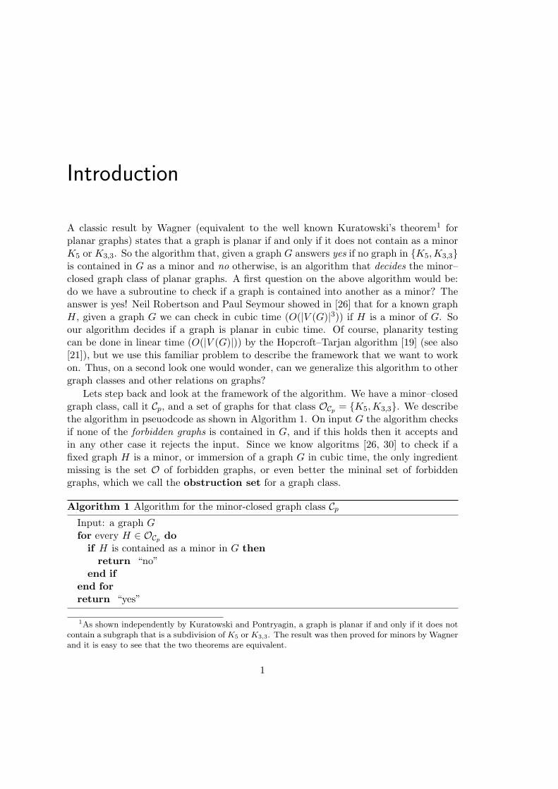
A classic result by Wagner (equivalent to the well known Kuratowski’s theorem1 forplanar graphs) states that a graph is planar if and only if it does not contain as a minorK5 or K3,3. So the algorithm that, given a graph G answers yes if no graph in {K5,K3,3}is contained in G as a minor and no otherwise, is an algorithm that decides the minor–closed graph class of planar graphs. A first question on the above algorithm would be:do we have a subroutine to check if a graph is contained into another as a minor? Theanswer is yes! Neil Robertson and Paul Seymour showed in [26] that for a known graphH, given a graph G we can check in cubic time (O(|V (G)|3)) if H is a minor of G. Soour algorithm decides if a graph is planar in cubic time. Of course, planarity testingcan be done in linear time (O(|V (G)|)) by the Hopcroft–Tarjan algorithm [19] (see also[21]), but we use this familiar problem to describe the framework that we want to workon. Thus, on a second look one would wonder, can we generalize this algorithm to othergraph classes and other relations on graphs?

Lets step back and look at the framework of the algorithm. We have a minor–closedgraph class, call it Cp, and a set of graphs for that class OCp = {K5,K3,3}. We describethe algorithm in pseuodcode as shown in Algorithm 1. On input G the algorithm checksif none of the forbidden graphs is contained in G, and if this holds then it accepts andin any other case it rejects the input. Since we know algoritms [26, 30] to check if afixed graph H is a minor, or immersion of a graph G in cubic time, the only ingredientmissing is the set O of forbidden graphs, or even better the mininal set of forbiddengraphs, which we call the obstruction set for a graph class.

Algorithm 1 Algorithm for the minor-closed graph class CpInput: a graph Gfor every H ∈ OCp do

if H is contained as a minor in G thenreturn “no”

end ifend forreturn “yes”

1As shown independently by Kuratowski and Pontryagin, a graph is planar if and only if it does notcontain a subgraph that is a subdivision of K5 or K3,3. The result was then proved for minors by Wagnerand it is easy to see that the two theorems are equivalent.

1

2 Introduction

Klaus Wagner conjectured2 that for every infinite set of finite graphs, one of itsmembers is a minor of another i.e. the minor relation on finite graphs is a well–quasi–order (WQO). And that (Robertson and Seymour theorem, Graph Minor Theorem,GMT, [27], 2004) was proved in a series of papers by Robertson and Seymour, calledthe Graph Minors (1983–2010). Later on, in [30] the immersion relation was also provento be a well–quasi–order. Consequently, every minor or immersion-closed graph classhas a finite obstruction set. Thus, we have the last ingredient to generalize Algorithm1 but are we done? Unfortunately, the answer here is no! And it is negative becausethe GMT guarantees the existense of a finite obstruction set, but since the proof isnon-constructive [23], it gives us no algorithm to construct the obstruction set.

The natural question that arises is

“what pieces of information do we need for a minor or immersion-closedgraph class to transform the existense of the obstruction set to a constructionof it?”

M.R. Fellows and M. Langston proved in [16] that an algorithm for deciding membershipin a minor-closed graph class F is not sufficient to construct the obstruction set of F .However, the results of “On computing graph minor obstruction sets” by K. Cattell, M.J.Dinnen, R.G. Downey, M.R. Fellows and M.A. Langston, [6], and “Computing ExcludedMinors” by I. Adler, M. Grohe and S. Kreutzer, [1], showed that there are algorithmsthat compute obstruction sets of minor-closed graph classes, but for that we need moreinformation than just an algorithm for membership in F .

The approach of Cattell et al. is an algorithmic one. The authors employ an analogueof the Myhill–Nerode theorem [15] and define congruences based on a minor–closed classthat split the class in a finite number of equivalence classes, of which they find the mininalelements. They demand the knwoledge of a bound on the treewidth of the obstructionsbut another algorithm for obstruction set computation is also proven, demanding otherinformation about the congruence but not the bound on the treewidth. The approachof Adler et al. requires that the minor–closed graph class we examine is definable inlayerwise monadic second–order logic (layerwise MSO). Again a bound on the treewidthof the obstructions is needed and Seese’s theorem [31] plays an important role. We aregoing to present these two approaches in chapter 3 and 4 respectively.

A main application given in both of the papers is the computation of the obstructionset of F1 ∪ F2 given the obstruction set of two minor-closed graph classes, F1 and F2.Using some of the machinery of [1], A. Giannopoulou, D. Zoros and the author, under thesupervision of our advisor D.M. Thilikos, proved that there is an algorithm to computethe obstruction set of F1 ∪ F2 given the obstruction set of two immersion–closed graphclasses, F1 and F2. This work was published on SWAT 2012 and is presented in chapter5, in the scope of computability, as an application of the previous chapters. Chapter 5ends with some concluding remarks, and of course all the basic notions and preliminariesare presented in chapter 2.

2The conjecture is known to be Wanger’s, but Wagner has said that he never made this conjecture! [12]

3

But have we solved the problem of constructibility of the obstruction sets? Theanswer is almost yes. And that is, because eventhough we have algorithms to computethe obstruction sets of minor and immersion-closed graph classes, the running time ofthese algorithms is not constructive. This means that we know that our algorithms willstop having produced the obstruction set, but we don’t know when. This problem is stillopen and we are not sure if we can bound the running time of the algorithms or not.

4 Introduction

Chapter 1

Preliminaries

1.1 Basics

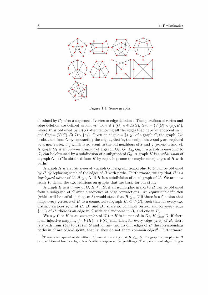
Lets begin with the definitions of some basic notions. N, Z and R denote the setsof natural numbers, integers and real numbers respectively. By [n] we denote the set{1, . . . , n} of the first n integers. A (simple) graph G is defined to be an ordered pair(V,E) consisting of two sets: the set of vertices (or nodes) V or V (G) and the setof edges E or E(G), where an edge is a two-element set including elements from V :E ∈ {X ⊂ P(V ) | ∀e ∈ X : |e| = 2}. Schematically, we draw graphs by representing theelements of V as (labeled) nodes and the edges with lines between the two correspondingnodes (endpoints). In figure 1.1 we can see some examples of graphs.

A directed graph is a simple graph where the edges are not sets but ordered pairs,i.e. elements of V ×V , and a weighted graph is a simple graph where a real number (theweight) is assigned to each edge. We are going to deal with graphs that are undirected,unweighted and contain no loops (edges with the same endpoints) or multiple edgesbetween two vertices (E is a set, so an edge {v1, v2} can connect two vertices at mostonce).

In a graph G = (V,E) the degree of a vertex v is the number of its neighbours.We write degG(v) = |{w ∈ V | {v, w} ∈ E}|. The maximum degree of G = (V,E),is ∆(G) = max{degG(v) | v ∈ V } and its line graph is the graph L(G) = (E,X),where X = {{e1, e2} | e1, e2 ∈ E ∧ e1 ∩ e2 = ∅ ∧ e1 = e2}. Two graphs G1 = (V1, E1)and G2 = (V2, E2) are isomporphic if there is a bijection1 f from V1 to V2, such that{v, w} ∈ E1 ⇔ {f(v), f(w)} ∈ E2. For example try to see that all graphs in figure 1.1are isomporphic2. Given two graphs G and H, the lexicographic product G ×H, is thegraph with V (G × H) = V (G) × V (H) and E(G × H) = {{(x, y), (x′, y′)} | ({x, x′} ∈E(G)) ∨ (x = x′ ∧ {y, y′} ∈ E(H))}.

Now lets continue with relations on graphs. We say that a graph G1 = (V1, E1)is a subgraph of a graph G2 = (V2, E2), G1 ⊆ G2, if a graph isomorphic to G1 can be

1A one-to-one and onto function.2The first graph of figure 1.1 is called the Petersen graph. Eventhough all graphs in figure 1.1 are

isomorphic its first draw is more popular.

5

6 1. Preliminaries

Figure 1.1: Some graphs.

obtained by G2 after a sequence of vertex or edge deletions. The operations of vertex andedge deletion are defined as follows: for v ∈ V (G), e ∈ E(G), G\v = (V (G) ∖ {v}, E′),where E′ is obtained by E(G) after removing all the edges that have an endpoint in v,and G\e = (V (G), E(G)∖ {e}). Given an edge e = {x, y} of a graph G, the graph G\eis obtained from G by contracting the edge e, that is, the endpoints x and y are replacedby a new vertex vxy which is adjacent to the old neighbors of x and y (except x and y).A graph G1 is a topological minor of a graph G2, G1 ≤tp G2, if a graph isomorphic toG1 can be obtained by a subdivision of a subgraph of G2. A graph H is a subdivision ofa graph G, if G is obtained from H by replacing some (or maybe none) edges of H withpaths.

A graph H is a subdivision of a graph G if a graph isomorphic to G can be obtainedby H by replacing some of the edges of H with paths. Furthermore, we say that H is atopological minor of G, H ≤tp G, if H is a subdivision of a subgraph of G. We are nowready to define the two relations on graphs that are basic for our study.

A graph H is a minor of G, H ≤m G, if an isomorphic graph to H can be obtainedfrom a subgraph of G after a sequence of edge contractions. An equivalent definition(which will be useful in chapter 3) would state that H ≤m G if there is a function thatmaps every vertex v of H to a connected subgraph Bv ⊆ V (G), such that for every twodistinct vertices v, w of H, Bv and Bw share no common vertex, and for every edge{u, v} of H, there is an edge in G with one endpoint in Bv and one in Bu.

We say that H is an immersion of G (or H is immersed in G), H ≤im G, if thereis an injective mapping f : V (H) → V (G) such that, for every edge {u, v} of H, thereis a path from f(u) to f(v) in G and for any two disjoint edges of H the correspondingpaths in G are edge-disjoint, that is, they do not share common edges3. Furthermore,

3There is an equivalent definition of immersion stating that H ≤im G, if a graph isomorphic to Hcan be obtained from a subgraph of G after a sequence of edge–liftings. The operation of edge–lifting is

1.2. WQO, GMT AND OBSTRUCTIONS 7

two paths are called vertex-disjoint if they do not share common vertices. Naturally,the above relations on graphs also define orderings on graphs (e.g. minor ordering,immersion ordering).

1.2 WQO, GMT and obstructions

Definition 1.1. A well-quasi-ordering, WQO, on a set C is a quasi-ordering (a reflexiveand transitive binary relation) which has no infinite descending sequences and no infiniteantichains.

An infinite antichain in C is an infinite sequence of elements in C such that for everyxi, xj ∈ C, with i < j, we have that xi ≰ xj . For example, we know by Kruskal’s TreeTheorem [22] that the set of rooted trees is WQO by the topological minor relation.

Theorem 1.2 (Graph Minor Theorem, [27]). The class of finite graphs is well-quasi-ordered by the minor relation.

Robertson and Seymour in the last of the Graph Minors series also proved the fol-lowing:

Theorem 1.3 ([30]). The class of finite graphs is well-quasi-ordered by the immersionrelation.

Definition 1.4. Let ≤ be a relation on graphs, such as ≤m or ≤im. A graph class C is≤–closed, or closed under ≤, if for every graph G in C, if H ≤ G for a graph H, thenH also belongs to C.

As an example, consider the class of planar graphs, Cp. If G is planar and H ≤m G,then H is also planar, since vertex and edge deletion and edge contraction preserveplanarity. So Cp is a minor–closed graph class. Since edge lifting also preserves planarity,Cp is also an immersion-closed graph class.

Definition 1.5. The obstruction set of a ≤–closed graph class C, obs(C), is the minimalset of graphs H satisfying the following property:

G ∈ C ⇔ for every H ∈ H, H ≰ G

As a corollary of theorems 1.2 and 1.3, we get the following:

Corollary 1.6. For every minor or immersion–closed graph class C, the set obs(C) isfinite.

It is obvious that if a graph class C is minor–closed and also immersion–closed, theminor obstructions obsm(C) are not the same with the immersion obstructions obsim(C),except for some trivial cases. In addition, obstruction sets are often large sets of graphs.As an example we give the following theorem (we will not define tree–depth since thistheorem is given only as an example of the cardinality of an obstruction set).

the replacement of two edges {v, x}, {x,w} with a new one {v, w}.

8 1. Preliminaries

Theorem 1.7 (A. Giannopoulou and D.M. Thilikos, [18]). Let F be the (≤m–closed)

class of all graphs with tree-depth at most k. Then |O| ≥ 22k−(2k+1) + 22

k−(k+1), whereO is the obstruction set of the class.

1.3 Treewidth

This section is about a parameter on graphs called treewidth, introduced by N. Robertsonand P. Seymour in [25]. Intuitively this parameter indicates how much a graph resemblesa tree. For a formal approach we have to define tree decompositions.

A tree decomposition of a graph G is a pair (T,B), where T is a tree and B is afunction that maps every vertex v ∈ V (T ) to a subset Bv of V (G) such that:

(i) for every edge e of G there exists a vertex t in T such that e ⊆ Bt,

(ii) for every v ∈ V (G), if r, s ∈ V (T ) and v ∈ Br ∩Bs, then for every vertex t on theunique path between r and s in T , v ∈ Bt and

(iii)∪

v∈V (T )

Bv = V (G).

We usually treat a node t of T and the corresponding set of vertices B(t) as equal.So when we refer to the vertices in t of T it will be clear that we mean B(t).

The width of a tree decomposition (T,B) is width(T,B) := max{|Bv|−1 | v ∈ V (T )}and the treewidth of a graph G, tw(G), is the minimum over the width(T,B), where(T,B) is a tree decomposition of G.

If on the above definition we restrict T to be a path, we define path decompositionand pathwidth, pw(G).

A graph class C is said to have bounded treewidth if there is a k ∈ N, such that forevery graph G in C, tw(G) ≤ k.

Despite the fact that treewidth will play a key role in both approaches studied for ob-struction set computation, it is a parameter with a wide impact on theoretical computerscience and therefore well studied. Many NP-hard problems on graphs become polyno-mial time solvable when we know a bound on the treewidth, with exact algorithms orapproximate. For example, computing the maximum independent set4 of a graph is aclassic NP-complete problem and it is also hard to approximate.

Theorem 1.8 (Arnborg and Proskurowski [2]). The size of the largest independent setin a graph of treewidth k can be computed in O(4kk2n) time.

In both approaches studied to compute the obsrtuction set of a graph class C weare going to require for obs(C) to have bounded treewidth. This bound always exists,since the obstruction sets of minor or immersion–closed graph classes are finite. On theother hand, there are many graph classes that have themselves bounded treewith and

4An independent set of a graph G is a subset X of its vertices, such that no two vertices in X areadjacent in G.

1.3. TREEWIDTH 9

as an example we give the following theorem (for a proof of the theorem and a study ontreewidth see [14]).

Theorem 1.9. A minor-closed family of graphs has bounded treewidth if and only if itexcludes at least one planar graph.

On the contrary, there are many classes with no bounded treewidth. A simpleexample is, again, the minor–closed class of planar graphs, Cp. All the grid graphs(Pn × Pm, n,m ∈ N, × is the graph Cartesian product and Pi is a path with i nodes)are included in Cp, but since tw(Pn × Pn) = n, for any n ∈ N we can find a graph in Cpwith treewidth exactly n. For a survey on treewidth see [5].

10 1. Preliminaries

Chapter 2

An algorithmic approach

In [6] K. Cattell, M. Dinneen, R. Downey, M. Fellows and M. Langston present algo-rithms for obstruction set computation of minor–closed graph classes, which they callideals, remarking that their methods can be adapted to other partial–orders on graphssuch as immersions and topological orders. The first algorithm appeared in [15] (but itscorrectness was fully proved for the first time in [6]) and is based on the Myhill–Nerodetheorem for regular languages. However, an upper bound of the treewidth of the ob-structions is an essential ingredient of the algorithm and this piece of information is notalways known. Thus, the authors introduce the notion of second–order congruence for agraph property, which allows them to compute the obstruction set of an ideal requiringother information (about the congruence) but not the upper bound of the treewidth ofthe obstructions. In this chapter we present these algorithms.

2.1 Introduction

The first algorithm is an analogue of the Myhill–Nerode theorem ([15]), but beforerecalling the theorem it is necessary to define some relevant notions. Let L ⊆ Σ∗ bea language and ∼ an equivalence relation. The canonical equivalence relation ∼L is,x ∼L y if and only if, ∀z ∈ Σ∗, xz ∈ L ⇐⇒ yz ∈ L. We say that ∼ is a congruenceif, ∀z ∈ Σ∗, x ∼ y ⇐⇒ xz ∼ yz and zx ∼ zy. We can now state the Myhill–Nerodetheorem.

Theorem 2.1 (Myhill–Nerode). Let L ⊆ Σ∗. If an equivalence relation ∼ that isdecidable with a known algorithm satisfies the following:

(1) ∼ has finite index

(2) ∼ is a congruence with respect to concatenation

(3) x ∼ y =⇒ x ∼L y,

then L is regular and an algorithm is known to compute a DFA1 that recognizes L.

1Deterministic Finite Automaton.

11

12 2. An algorithmic approach

Instead of words and languages over an alphabet we deal with graphs and graphclasses. To define an operation analogous to concatenation2 we have to define t-boundaried graphs in order to “glue” graphs together (on the boundary), as concatena-tion does with words.

Definition 2.2. A t-boundaried graph G = (V,E,B, f) is a simple graph G = (V,E)together with:

(i) a subset of vertices B ⊆ V , which we call the boundary, such that |B| = t

(ii) a bijection f : B → {1, . . . , t} (a labeling of the boundary vertices)

We denote by U tlarge the set of all t–boundaried graphs and by G = (V,E) the

underlying graph of the t–boundaried graph G = (V,E,B, f). For simplicity, sometimeswe will not distinguish between the t–boundaried graph and the the underlying graph.So for example when we write G ∈ F and G is a t–boundaried graph, we actually meanG ∈ F . We now define the following operation on t–boundaried graphs.

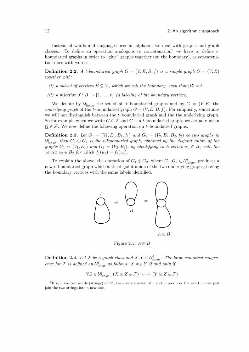
Definition 2.3. Let G1 = (V1, E1, B1, f1) and G2 = (V2, E2, B2, f2) be two graphs inU tlarge, then G1 ⊕ G2 is the t-boundaried graph, obtained by the disjoint union of the

graphs G1 = (V1, E1) and G2 = (V2, E2), by identifying each vertex u1 ∈ B1 with thevertex u2 ∈ B2 for which f1(u1) = f2(u2).

To explain the above, the operation of G1 ⊕ G2, where G1, G2 ∈ U tlarge, produces a

new t–boundaried graph which is the disjoint union of the two underlying graphs, havingthe boundary vertices with the same labels identified.

⊕

A

B

A⊕B

=

Figure 2.1: A⊕B

Definition 2.4. Let F be a graph class and X,Y ∈ U tlarge. The large canonical congru-

ence for F is defined on U tlarge as follows: X ≈F Y if and only if,

∀Z ∈ U tlarge : (X ⊕ Z ∈ F) ⇐⇒ (Y ⊕ Z ∈ F)

2If v, w are two words (strings) of Σ∗, the concatenation of v and w produces the word vw–we justjoin the two strings into a new one.

2.1. INTRODUCTION 13

Definition 2.5. The small treewidth universe, U ttree, is the set of all t–boundaried graphs

having tree decomposition of width t − 1 (equivalently, treewidth3 at most t) for whichthe set of boundary vertices is the set of vertices indexed by the root of the tree.

The small pathwidth universe, U tpath, is the set of all t–boundaried graphs having a

path decomposition of width t − 1 (equivalently, pathwidth4 at most t) for which the setof boundary vertices is the last set of the decomposition.

When our statements hold for both U ttree and U t

path we will simply write U tsmall. We

remark that if G is a graph in U ttree (resp. U t

path) the trees (resp. paths) of a minimaltree (resp. path) decomposition of G are rooted and the root of the tree (resp. end ofthe path) has size exactly t. The following simple lemma will be useful in the sequel.

Lemma 2.6. Let A,B ∈ U tsmall. Then tw(A⊕B) ≤ t (equiv. pw(A⊕B) ≤ t).

Proof. Let A,B ∈ U ttree (the same arguements hold for the case of U t

path). We consider atree decomposition (T1, B1) of A and a tree decomposition (T2, B2) of B such that bothdecompotitions have width t − 1 and the set of boundary vertices is the set of verticesindexed by the root of every tree. We concider the tree T which occurs from the disjointunion of the trees T1 and T2 by identifying their roots, which is also the root of T , and wename the boundary vertices of A and B with their labels in {1, . . . , t}. We also considerthe function B which is the union of B′

1 and B′2, where B

′i is the function Bi having

replaced any occurence of a boundary vertex with its label. Then it is easy to check that(T,B) is a tree decomposition of A ⊕ B and therefore tw(A ⊕ B) ≤ t (in the case ofU tpath we would join the ends of the paths of the path decompositions of A and B).

Similarly with ≈F (definition 2.4) we define the small canonical congruence ∼F inU tsmall.

Definition 2.7. Let X,Y ∈ U tsmall. The small canonical congruence is defined by

X ∼F Y if and only if

∀Z ∈ U tsmall : (X ⊕ Z ∈ F) ⇐⇒ (Y ⊕ Z ∈ F)

We denote by [x]∼ the equivalence class of x with respect to ∼ and we say that ∼has finite index on U , if ∼ has a finite number of equivalence classes in U . We say that∼ refines ≈, where ∼ and ≈ are two equivalence relations in U , if

∀x, y ∈ U : x ∼ y =⇒ x ≈ y

If we consider ∼F and ≈F it is trivial to see that ≈F refines ∼F (the two relationsthough, might not coincide). Finally, it is shown in [11] that on U t

tree the large canonicalcongruence ≈F has finite index if and only if the small canonical congruence ∼F hasfinte index, for a graph class F .

3For a t-boundaried graph G, tw(G) = tw(G).4As above, for G ∈ U t

large, pw(G) = pw(G).


2.2 An algorithm for obs(F)

After defining the analogous notions of the Myhill–Nerode theorem (2.1) for graphs, wecan now state an analogue of the theorem, which is the first algorithm in our study forobstruction set computation.

Theorem 2.8 ([6]). Let F be a minor closed graph class. If we have the following threepieces of information:

(i) An algorithm to decide membership in F (of any time complexity).

(ii) A bound B on the maximum treewidth of the obstructions for F .

(iii) For t = 1, . . . , B + 1 a decision algorithm for a finite–index congruence ∼ on t–boundaried graphs that refines the small canonical congruence for F .

Then we can effectively compute the obstruction set O for F .

Proof. In short, the information given are enough to bound the search space of theobstructions and by using the algorithm for F–membership we find the minimal graphs(with respect to an ordering that will be defined) that do not belong to F , i.e. theobstructions of F . We can now state the algorithm and then explain it and prove itscorrectness.

Algorithm 2 obs(F) computation

for t = 1, . . . , B + 1 doj ← 1while a stop signal is not detected do

generate all graphs of the jth generation and store them in Gtj ← j + 1

end whilestore all the ≤–mininal graphs of Gt inMt

for every G ∈Mt doif G /∈ F then store G in Ot

end forend for

returnB+1∪t=0Ot

Algorithm 2 has two loops. The outer loop t = 1, . . . , B + 1 specifies that we arecurrently working in U t

tree. In the inner loop the graphs of U ttree are generated, until a

stop signal is detected and all these graphs are stored in Gt. When this process ends,we store all the ≤–minimal graphs of Gt in Mt (≤ will be defined in the sequel) andthis process is completed in a finite number of steps, since Gt is finite. Then, by us-ing the algorithm for F–membership we discard all the underlying graphs of Mt that

2.2. AN ALGORITHM FOR OBS(F) 15

belong to F and store the remaining elements ofMt in Ot. Since Ot contains all the ≤–

minimal graphs of U ttree that do not belong in F , the algorithm ends by returning

B+1∪t=0Ot,

which is (as we will prove in the sequel) the obstruction set of F (the obstruction set ofa class F can be also defined as the set of all ≤–minimal graphs of the complement of F).

To complete the description of the algorithm we need to explain (a) how the graphsof the inner loop are generated (what is the jth generation in Algorithm 2), (b) the ≤ordering, and (c) the stop signal.

For (a) we define size(X), where X ∈ U ttree, to be the number of nodes in the smallest

possible rooted tree of a tree–decomposition for X such that the set of boundary verticesis indexed by the root of the tree5. By the term jth generation we mean the set ofgraphs of U t

tree of size j. This set is finite since a graph G ∈ U ttree of size j has a tree

decomposition (T,B) such that |V (T )| = j and tw(G) ≤ t, so G can have at most j(t+1)nodes and there are finitely many graphs with at most j(t+ 1) nodes.

To clarify (b) we firstly extend the minor ordering ≤m to a minor ordering for t–boundaried graphs, ≤∂m. For H,G ∈ U t

tree, H ≤∂m G if a graph isomorphic6 to Hcan be obtained from G by a sequence of vertex deletions of non boundary vertices,edge deletions, and edge contractions of edges that have at least one non–boundaryendpoint. In fact, ≤∂m is a restriction of ≤m, where we can apply the graph operationsthat procude a minor in a way that leaves the boundary vertices unaffected: if H ≤∂m Gthen B = BH , where H = (VH , EH , BH , fH) and G = (V,E,B, f). The ≤∂m orderingcan easily be shown to be a WQO on U t

large by using the Graph Minor Theorem for

edge–colored graphs. Let X,Y ∈ U ttree, we define X ≤ Y if and only if X ≤∂m Y and

X ∼ Y . Since there are finitely many equivalence classes of ∼ (by hypothesis) and ≤∂m

is a WQO, ≤ is a WQO on U ttree.

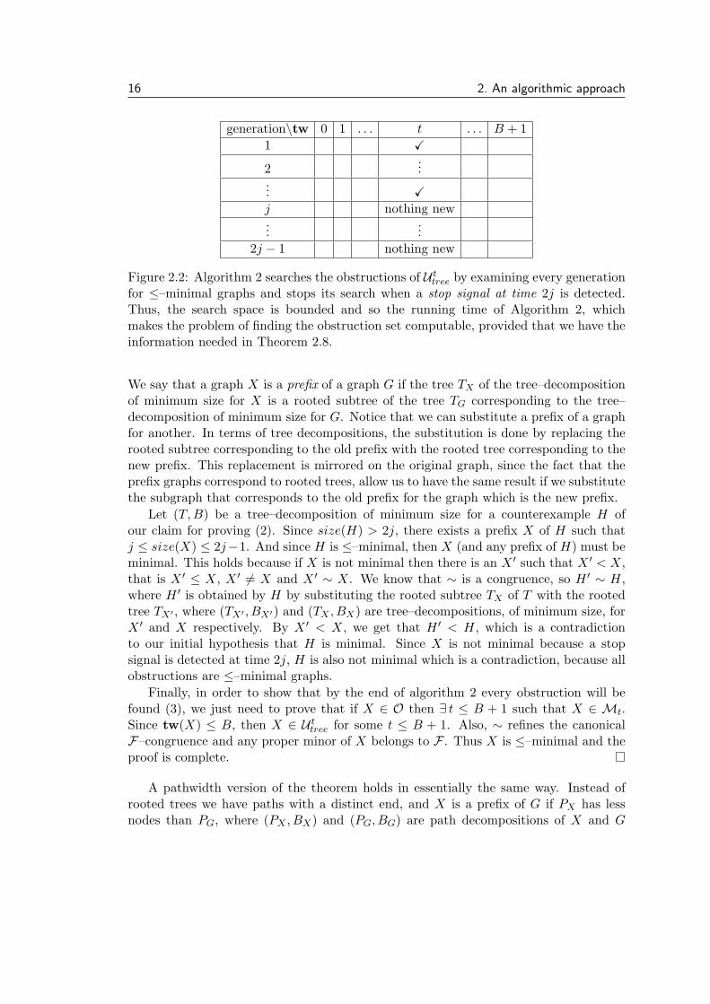
And for (c), we say that there is nothing new at time j if none of the t–boundariedgraphs of the jth generation are minimal with respect to the search ordering ≤. A stopsignal is detected at time 2j if there is nothing new at time i for i = j, . . . , 2j − 1 (seeFigure 2.2).

To end the proof we need to prove the correctness of the algorithm. For this we needto prove that (1) a stop signal will be met eventually for every t = 0, . . . , B + 1, (2) thestop signal is valid, which means that all the obstructions in U t

tree will be found until thestop signal will be met, and (3) all obstructions will be found by the end of Algorithm 2.

For (1), we know that ≤ is a WQO on U ttree, so there is a finite number of minimal

elements for the algorithm to search for.To prove (2), which is the most crucial part of this proof, we have to show that if for

a given t a stop signal is detected, then no obstruction for F , has size greater than 2j.

5In this proof all the trees of the tree–decompositions are as described in the definition of size(X).That is, the root of the tree contains all the boundary vertices.

6If G = (V,E,B, f) and G′ = (V ′, E′, B′, f ′) are two t–boundaried graphs, then G and G′ areisomorphic if there is a bijection g : V → V ′, such that {v1, v2} ∈ E ⇐⇒ {g(v1), g(v2)} ∈ E′,v ∈ B ⇐⇒ g(v) ∈ B′ and for every v ∈ B, f(v) = f ′(g(v)).


generation\tw 0 1 . . . t . . . B + 1

1 ✓2

...... ✓j nothing new...

...

2j − 1 nothing new

Figure 2.2: Algorithm 2 searches the obstructions of U ttree by examining every generation

for ≤–minimal graphs and stops its search when a stop signal at time 2j is detected.Thus, the search space is bounded and so the running time of Algorithm 2, whichmakes the problem of finding the obstruction set computable, provided that we have theinformation needed in Theorem 2.8.

We say that a graph X is a prefix of a graph G if the tree TX of the tree–decompositionof minimum size for X is a rooted subtree of the tree TG corresponding to the tree–decomposition of minimum size for G. Notice that we can substitute a prefix of a graphfor another. In terms of tree decompositions, the substitution is done by replacing therooted subtree corresponding to the old prefix with the rooted tree corresponding to thenew prefix. This replacement is mirrored on the original graph, since the fact that theprefix graphs correspond to rooted trees, allow us to have the same result if we substitutethe subgraph that corresponds to the old prefix for the graph which is the new prefix.

Let (T,B) be a tree–decomposition of minimum size for a counterexample H ofour claim for proving (2). Since size(H) > 2j, there exists a prefix X of H such thatj ≤ size(X) ≤ 2j−1. And since H is ≤–minimal, then X (and any prefix of H) must beminimal. This holds because if X is not minimal then there is an X ′ such that X ′ < X,that is X ′ ≤ X, X ′ = X and X ′ ∼ X. We know that ∼ is a congruence, so H ′ ∼ H,where H ′ is obtained by H by substituting the rooted subtree TX of T with the rootedtree TX′ , where (TX′ , BX′) and (TX , BX) are tree–decompositions, of minimum size, forX ′ and X respectively. By X ′ < X, we get that H ′ < H, which is a contradictionto our initial hypothesis that H is minimal. Since X is not minimal because a stopsignal is detected at time 2j, H is also not minimal which is a contradiction, because allobstructions are ≤–minimal graphs.

Finally, in order to show that by the end of algorithm 2 every obstruction will befound (3), we just need to prove that if X ∈ O then ∃ t ≤ B + 1 such that X ∈ Mt.Since tw(X) ≤ B, then X ∈ U t

tree for some t ≤ B + 1. Also, ∼ refines the canonicalF–congruence and any proper minor of X belongs to F . Thus X is ≤–minimal and theproof is complete.

A pathwidth version of the theorem holds in essentially the same way. Instead ofrooted trees we have paths with a distinct end, and X is a prefix of G if PX has lessnodes than PG, where (PX , BX) and (PG, BG) are path decompositions of X and G

2.3. OVERCOMING TREEWIDTH BOUND 17

respectively. In addition, an immersion version of the theorem can be proven, again inthe same way, but we have to define the ordering ≤ on t–boundaried graphs in terms ofimmersions. That is, H ≤ G, iff H ≤∂im G and H ∼ G. And ≤∂im is a restriction of≤im that preserves the boundary. That is, H ≤∂im G if a graph isomporphic to H canbe obtained from G by applying a sequence of vertex deletions of non–boundary vertices,edge deletions and edge liftings. Finally, Algorithm 2 has been implemented and someresults can be found in [9] and [8].

Knowing a bound on the treewidth of the obstructions was essential informationfor Algorithm 2, in terms of bounding the search space for the obstructions. However,neither such a bound is always known, nor a generic way to find it. So, in the nextsection we will try to overcome this difficulty by employing various stop signals.

2.3 Overcoming treewidth bound

Our first attempt to design an algorithm for obstruction set computation without theknowledge of a bound on the obstructions treewidth is, in a way, a generalization ofAlgorithm 2. The search is done in the same way but the whole prosess stops differently.For this we have to define a notion that will be usefull in the sequel, the alarm.

Definition 2.9. An alarm for a minor–closed class F is a pair of computable functions:

(1) fa : N→ N, and

(2) a : N→ {0, 1}, satisfying:

(a) (reliability) a(t)=1 if there is an obstruction H ∈ O∖Ot of pathwidth more thanfa(t)

(b) (eventual quiescence) ∃t0 such that ∀t ≥ t0, a(t) = 0.

We also have to point out that in this and the following sections of this chapter we willbe working in U t

path.

Theorem 2.10. If the following are known for a minor–closed graph class F :

(1) A decision algorithm for F–membership.

(2) A decision algorithm for a finite–index congruence for F (the congruence can beeither large or small).

(3) Algorithms for computing a and fa for an alarm for F .

then the obstruction set O of F can be computed.

Proof. For every t we compute Ot using the methods of the proof of Theorem 2.8(adapted to pathwidth computations), namely (1) and (2). That is, we have two (while)loops, the outer to specify the pathwidth and the inner to specify the generation and atthe end of every itteration of the outer loop, the underlying graphs of the ≤–minimal


elements of U tpath enumerated that do not belong to F are stored in Ot. For a certain

pathwidth t, the inner loop stops exactly as described in the proof of Theorem 2.8. Sincewe don’t know a bound on the pathwidth of the F–obstructions we will employ a certainstop signal to halt the outer loop (the one that specifies the pathwidth).

We say that a t-stop signal is detected if

(a) Oi = Ot for i = t, . . . , fa(t), and

(b) a(t)=0

Using the t-stop signal we compute the F–obstructions as described in Algorithm 3.

Algorithm 3 obs(F) computation

t← 0while a stop signal is not detected do

compute Oi, for i = t, . . . , fa(t) and a(t)t← t+ 1

end whilereturn Ot

In order to prove that the algorithm is correct we have to show that (a) if O = Ot

then there will be no t-stop signal, and (b) eventually a t-stop signal will be met.For (a) we have to examine two cases:(1) There exists an obstruction H ∈ O ∖Ot for which pw(H) ≤ fa(t). In this case thefirst condition of the t-stop signal will fail.(2) There exists an obstruction H ∈ O ∖Ot for which pw(H) > fa(t). In this case, bythe reliability of the alarm (definition 2.9) we have that a(t) = 1, so the second conditionof the t-stop signal will fail.

For (b), let t′ be the maximum pathwidth of the obstructions for F . Then fori = t′, . . . , fa(t

′) we have that Oi = Ot′ (since for every i ≥ t′, Oi = Ot′) and a(t′) = 0,since there is no obstruction with pathwidth more than t′. Thus, a t′-stop signal will bemet and Algorithm 3 will stop having correctly computed the obstruction set O = Ot′

of F .

Theorem 2.10 actually gives the general framework that we use for obstruction setcomputation. In that sense we can see theorem 2.8 as a special case of theorem 2.10, butour goal is to have an alarm that does not depend on the bound of the treewidth of theobstructions. To accomplish that we will employ a terminating second–order congruenceas an alarm. Before that, we give the necessary definitions.

Definition 2.11. The canonical second–order congruence for a minor–closed graph classF , ≈F , is defined on finite subsets of t–boundaried graphs in U t

large as follows: if S1, S2 ⊆U tlarge then S1 ≈F S2 if and only if

∀Z ∈ U tlarge : (∀X1 ∈ S1 : X1 ⊕ Z ∈ F) ⇐⇒ (∀X2 ∈ S2 : X2 ⊕ Z ∈ F)

2.3. OVERCOMING TREEWIDTH BOUND 19

Definition 2.12. Let ∼ be an equivalence relation defined on finite subsets of U tlarge. ∼

is a second–order congruence if ≈F refines ∼, i.e. ∼ implies ≈F .

Notice that a second–order congruence ∼ defines a first–order congruence when re-stricted to singletons: {A1} ∼ {A2}, for A1, A2 ∈ U t

large. Thus the canonical second–order congruence restricted on signletons is actually the canonical first–order congruence(large canonical congruence).

Definition 2.13. Let ∼ be a second–order congruence defined on a minor–closed graphclass F and S(A) denote all the t–boundaried graphs H, such that H <∂m G, for A ∈U tlarge. Then ∼ is called terminating if it satisfies the condition: ∃t0 such that ∀t ≥ t0,

if A ∈ U tpath such that (1) pw(A) ≥ t0 and (2) |int(A)| ≥ t0, then {A} ∼ {S(A)}.

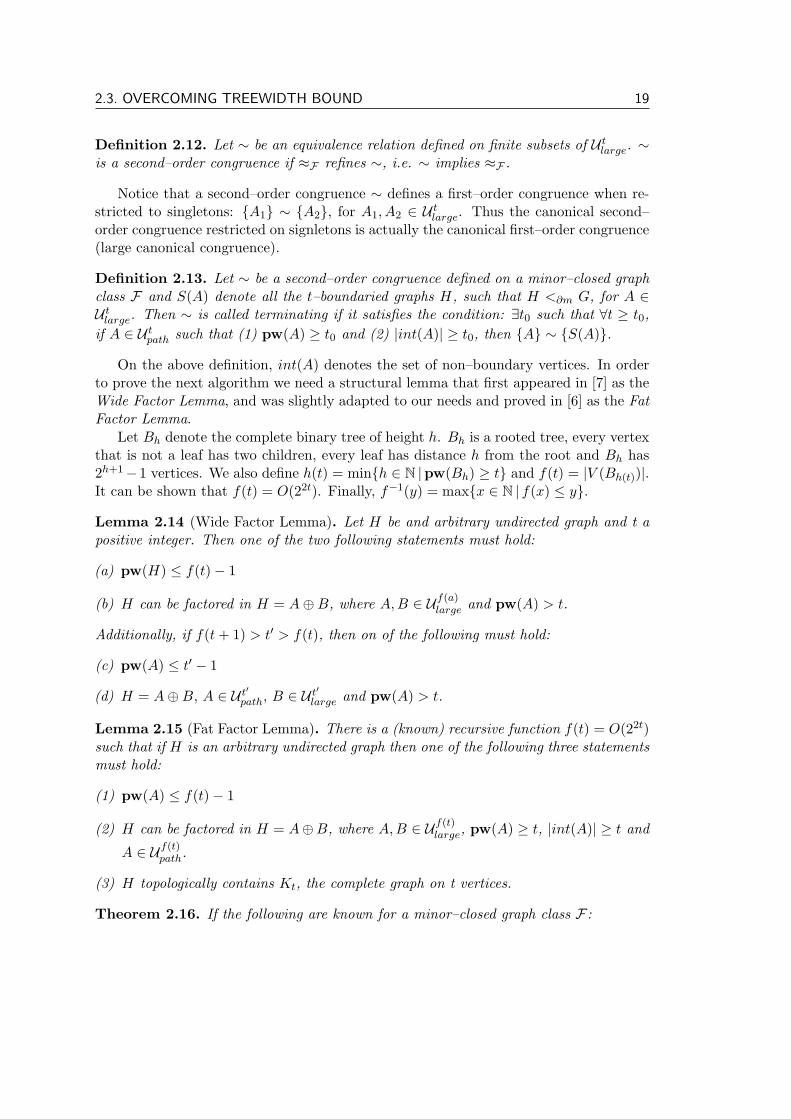
On the above definition, int(A) denotes the set of non–boundary vertices. In orderto prove the next algorithm we need a structural lemma that first appeared in [7] as theWide Factor Lemma, and was slightly adapted to our needs and proved in [6] as the FatFactor Lemma.

Let Bh denote the complete binary tree of height h. Bh is a rooted tree, every vertexthat is not a leaf has two children, every leaf has distance h from the root and Bh has2h+1−1 vertices. We also define h(t) = min{h ∈ N |pw(Bh) ≥ t} and f(t) = |V (Bh(t))|.It can be shown that f(t) = O(22t). Finally, f−1(y) = max{x ∈ N | f(x) ≤ y}.

Lemma 2.14 (Wide Factor Lemma). Let H be and arbitrary undirected graph and t apositive integer. Then one of the two following statements must hold:

(a) pw(H) ≤ f(t)− 1

(b) H can be factored in H = A⊕B, where A,B ∈ Uf(a)large and pw(A) > t.

Additionally, if f(t+ 1) > t′ > f(t), then on of the following must hold:

(c) pw(A) ≤ t′ − 1

(d) H = A⊕B, A ∈ U t′path, B ∈ U t′

large and pw(A) > t.

Lemma 2.15 (Fat Factor Lemma). There is a (known) recursive function f(t) = O(22t)such that if H is an arbitrary undirected graph then one of the following three statementsmust hold:

(1) pw(A) ≤ f(t)− 1

(2) H can be factored in H = A⊕B, where A,B ∈ Uf(t)large, pw(A) ≥ t, |int(A)| ≥ t and

A ∈ Uf(t)path.

(3) H topologically contains Kt, the complete graph on t vertices.

Theorem 2.16. If the following are known for a minor–closed graph class F :


(1) An algorithm for F–membership

(2) A decision algorithm for a terminating second–order congruence ≈ for F .

Then we can compute the obstruction set O for F (using the algorithms for (1) and (2)as subroutines).

Proof. Since we are trying to prove a 2.10–type theorem, Ot i.e. the obstructions ofpathwidth at most t is computed in exactly the same way as descirbed in the proof oftheorems 2.10 and 2.8. In particular, we compute all the minimal elements of U t

path withrespect to the order defined in the proof of theorem 2.8, i.e. A ≤ B iff A ≤∂m B andA ∼ B, where ∼ is the first–order congruence defined by the second–order congruenceof (2) resticeted to singletons: A ∼ B iff {A} ≈ {B}. This set is denoted by Mt andsince ≤ is a WQO (by the GMT) and ∼ has finite index it is also finite. Then by usingthe algorithm for (1) we compute Ot, which is the set of all underlying graphs of Mt

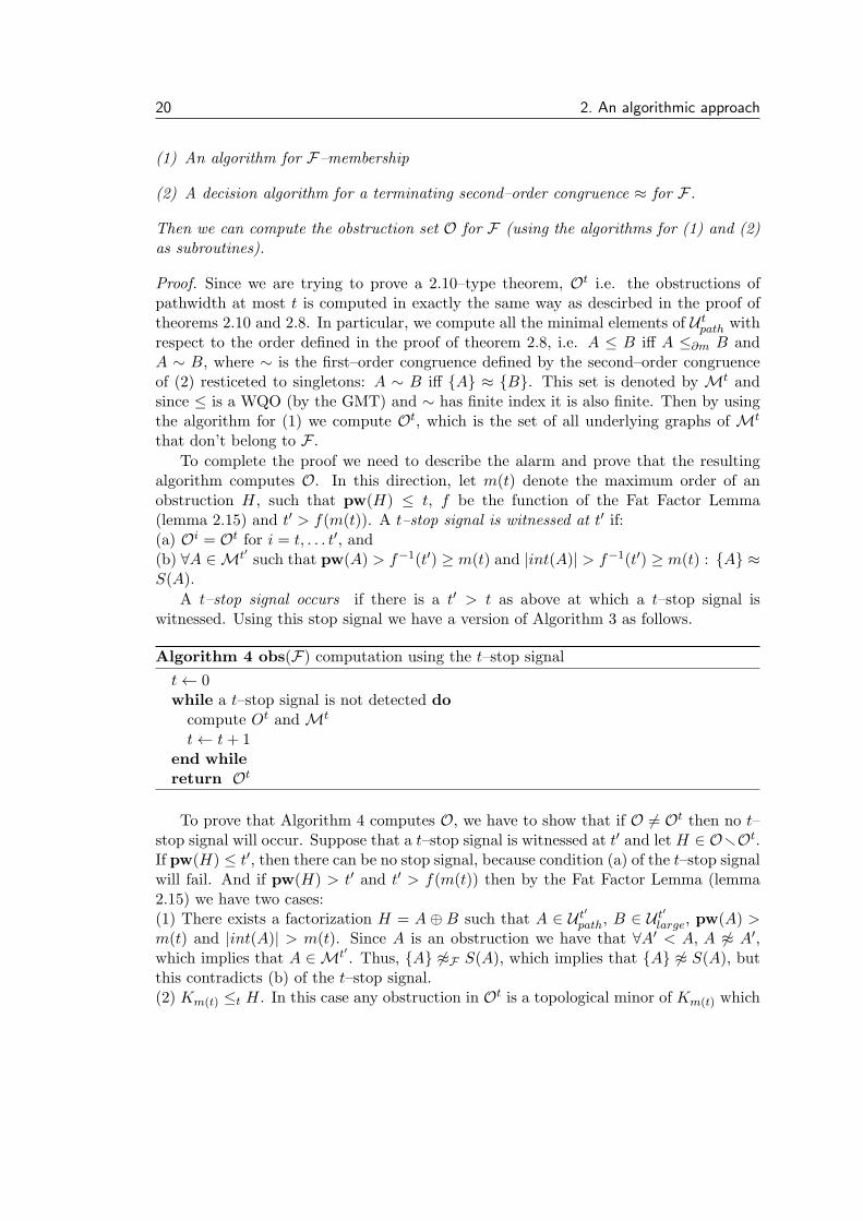
that don’t belong to F .To complete the proof we need to describe the alarm and prove that the resulting

algorithm computes O. In this direction, let m(t) denote the maximum order of anobstruction H, such that pw(H) ≤ t, f be the function of the Fat Factor Lemma(lemma 2.15) and t′ > f(m(t)). A t–stop signal is witnessed at t′ if:(a) Oi = Ot for i = t, . . . t′, and(b) ∀A ∈Mt′ such that pw(A) > f−1(t′) ≥ m(t) and |int(A)| > f−1(t′) ≥ m(t) : {A} ≈S(A).

A t–stop signal occurs if there is a t′ > t as above at which a t–stop signal iswitnessed. Using this stop signal we have a version of Algorithm 3 as follows.

Algorithm 4 obs(F) computation using the t–stop signal

t← 0while a t–stop signal is not detected do

compute Ot andMt

t← t+ 1end whilereturn Ot

To prove that Algorithm 4 computes O, we have to show that if O = Ot then no t–stop signal will occur. Suppose that a t–stop signal is witnessed at t′ and let H ∈ O∖Ot.If pw(H) ≤ t′, then there can be no stop signal, because condition (a) of the t–stop signalwill fail. And if pw(H) > t′ and t′ > f(m(t)) then by the Fat Factor Lemma (lemma2.15) we have two cases:(1) There exists a factorization H = A ⊕ B such that A ∈ U t′

path, B ∈ U t′large, pw(A) >

m(t) and |int(A)| > m(t). Since A is an obstruction we have that ∀A′ < A, A ≈ A′,which implies that A ∈ Mt′ . Thus, {A} ≈F S(A), which implies that {A} ≈ S(A), butthis contradicts (b) of the t–stop signal.(2) Km(t) ≤t H. In this case any obstruction in Ot is a topological minor of Km(t) which

2.4. APPLICATIONS & FINAL REMARKS 21

is a topological minor of H, so any obstruction in Ot is a topological minor of H, whichcontradicts the minimality of H.

Thus, if O = Ot, which will eventually happen since ≤ is a WQO, a stop signal willbe witnessed at time t′ = max{f(t0), f(m(t))}, where t0 is the termination constant,and the proof is complete.

To accomplish our goal for designing an algorithm for obstruction set computationwithout the knowledge of a bound on the treewidth of the F–obstructions we need toshow that there exists a terminating second–order congruence.

Theorem 2.17 ([6]). The canonical second–order congruence ≈F for a minor–closedgraph class F is terminating.

2.4 Applications & final remarks

As an application of the two main results of [6] (theorems 2.8 and 2.16–by using ≈Fas the terminating second–order congruence) the problem of computing the obstructionset O for a union of two minor–closed graph classes F = F1 ∪ F2 is studied. In thisproblem we are given the obstruction sets O1 and O2 of the minor–closed classes F1 andF2 respectively and our objective is to compute O. A weaker version of these problem issolved in [6], in which O can be computed by O1 and O2 and the use of Theorem 2.16,under the condition that O1 contains at least one tree7.

In [1] the union problem, among others, is solved without the aforementioned con-dition. The authors present a different technique for obstruction set computation, inwhich they demand the knowledge of a formula in Monadic Second–Order Logic (MSO)defining a minor–closed graph class F and a bound on the treewidth of the obstructionsof F . We are going to present these methods and their applications (e.g. union problem)in the next chapter.

7Actually, the condition we need is that a tree is contained in at least one of O1 and O2.

Chapter 3

Trying Monadic Second–Order Logic

In this chapter we present some of the results in [1] by I. Adler, M. Grohe and S. Kreutzer,for obstruction set computation of minor–closed graph classes. The main theorem thatis proven states that we can compute the obstruction set O of a minor–closed graph classF if we are given a formula φF in Monadic Second–Order Logic (MSO) that defines Fand an upper bound on width(F) (the bound on width(F) is related to the bound onthe treewidth of the obstructions for F). By applying these methods, the authors solve(among others) the union problem. That is, given the obstruction sets O1 and O2 oftwo minor–closed graph classes F1 and F2 respectively, we can effectively compute theobstruction set of their union F1 ∪ F2.

3.1 Graphs and Logic

Lets recall the alternative definition of graph minors in section 1.1. We say that H is aminor of G, H ≤m G, if there is a function that maps every vertex v of H to a connectedsubgraph Bv ⊆ V (G), such that for every two distinct vertices v, w of H, Bv and Bw

share no common vertex, and for every edge {u, v} of H, there is an edge in G with oneendpoint in Bv and one in Bu. The graph that is obtained by the union of all Bv suchthat v ∈ V (H) and by the edges between Bv and Bu in G, if there exists an edge {v, u}in H, is called a model of H in G. The model with the minimum number of verticesand edges is called minimal model. Obviously, if G′ is a minimal model of H in G, thenevery Bv in G′ is a tree with degH(v) leaves.

Lemma 3.1. Let k > 0 and H ≤m G, with |V (H)| = k. Then any minimal model G′

of H in G has tw(G′) ≤ k2 + 1.

Proof. To prove this lemma we have to recall the definition of models. A model consistsof k = |V (H)| mutually disjoint connected subgraphs of G corresponding to the verticesof H and of |E(H)| edges among them which correspond to the edges of H: there isan edge between Bu and Bv iff {u, v} is an edge of H. In a minimal model, the Bv

subgraphs are trees with at most degH(v) leaves. Let G′ be a minimal model of G. Ifwe consider the graph that is obtained by G′ by deleting all the edges among the Bv

23

24 3. Trying MSO

trees, v ∈ V (H), then the resulting graph is a forest (a union of trees) and has treewidthexactly 1. If we start putting back the edges that we removed, then every edge thatwe add can increase the treewidth at most by 1. Since we can add at most

(k2

)vertices

(k = |V (H)|) and the fact that when we add all the edges that we removed the resultinggraph will be again G′, we have that tw(G′) ≤

(k2

)+ 1 ≤ k2 + 1.

Corollary 3.2. For all graphs H, G, if H ≤m G then there exists a subgraph G′ of Gwith H ≤m G′, satisfying tw(G′) ≤ |V (H)|2 + 1.

By the Graph Minor Theorem and corollary 3.2, for every minor–closed graph classF there exists a w such that for every G /∈ F there exists a subgraph G′ of G, such thattw(G′) ≤ w. To see why this holds, firstly consider that, by the GMT, the obstruction setO of a minor–closed graph class F is finite. And for every G /∈ F , there exists an H ∈ Osuch that H ≤m G. Now if G′ is the minimal model of H in G, by corollary 3.2 we havethat tw(G′) ≤ |V (H)|2+1. Since O is finite, and if w = max{|V (H)|2+1 |H ∈ O} thenfor the (arbitrary) minor–closed class F and for every G /∈ F there exists a subgraphG′ of G such that tw(G′) ≤ |V (H)|2 + 1 ≤ w, where H is an obstruction such thatH ≤m G. Finally, since H ≤m G′, G′ /∈ F .

Definition 3.3. Let F be a minor–closed graph class. The least k such that for everyG /∈ F there exists a G′ ⊆ G with G′ /∈ F and tw(G′) ≤ k is called the width of F andis denoted by width(F).

We now recall some definitions from Monadic Second Order Logic (MSO). An ex-tended introduction to Logic can be found in [13, 24].

We call signature τ = {R1, . . . , Rn} any finite set of relation symbols Ri of any(finite) arity denoted by ar(Ri). For the language of graphs G we consider the signatureτG = {V,E, I} where V represents the set of vertices of a graph G, E the set of edges,and I = {(v, e) | v ∈ e and e ∈ E(G)} the incidence relation.

A τ -structure A = (A,RA1 , . . . , R

An) consists of a finite universe A, and the interpre-

tation of the relation symbols Ri of τ in A, that is, for every i, RAi is a subset of Aar(Ri).

For every graph we associate a relational structure G := (V (G)∪E(G), V G, EG, IG), overthe signature τG , where V

G = V (G), EG = E(G) and IG = {(v, e) | e ∈ E(G) and v ∈e∩V (G)}. A graph structure G is a τG-structure, which represents the graph G = (V,E).From now on, we abuse notation by treating G and G equally.

In MSO formulas are defined inductively from atomic formulas, that is, expressionsof the form Ri(x1, x2, . . . , xar(Ri)) or of the form x = y where xi, i ∈ [ar(Ri)], x and yare variables, by using the Boolean connectives ¬,∧,∨,→, and existential or universalquantification over individual variables and sets of variables. Furthermore, quantificationtakes place over vertex or edge variables or vertex-set or edge-set variables. Notice thatin the language of graphs the atomic formulas are of the form V (u), E(e) and I(u, e),where u and e are vertex and edge variables respectively.

Definition 3.4. A graph class C is MSO-definable if there exists an MSO formula φCin the language of graphs such that G ∈ C if and only if G |= φC, that is, φC is true inthe graph G (G models φC).

3.1. GRAPHS AND LOGIC 25

Lemma 3.5. The class of graphs that contain a fixed graph H as a minor is MSO–definable by an MSO–formula φH .

Proof. Let H = (V,E). Then the MSO–sentence φH is defined as ∃X1 . . . ∃Xkψ whereψ is the following sentence:(∧

i=j

Xi ∩Xj = ∅ ∧∧i(∅ ⊊ Xi ⊆ V ∧ “Xi is connected”∧

∧{vi,vj}∈E(H)

∃xi ∈ Xi∃xj ∈ Xj∃z((xi, z) ∈ I ∧ (xj , z) ∈ I)

)where “Xi is connected” can be expressed in MSO by the following formula:

∀u ∈ Xi∀v ∈ Xi∃{x1, . . . , xℓ} ⊆ Xi

(x1 = u ∧

ℓ−1∧i=1

{xi, xi+1} ∧ xu = v

)

Thus, H ≰m G iff G |= ¬φH . So if O is the obstruction set of a minor–closed classC, then if φO ≡

∨H∈O

φH we have that G ∈ C ⇐⇒ G |= ¬φO and ¬φO defines C.

The following theorem is basic for this chapter’s approch on obstruction set compu-tation algorithms.

Theorem 3.6 (Seese’s Theorem [31]). For every positive integer k, it is decidable givenan MSO–formula whether it is satisfied by a graph G whose tree–width is upper boundedby k.

Before we present the main theorem of this approach we have to extend the graphstructures we defined earlier to structures that are defined by a graph and its tree–decomposition. Intuitively a tree–dec expansion is a pair of two structures, one definedby the graph G and one defined by a tree decomposition (T,B) of G.

Definition 3.7. Let G = (V,E) be a graph and T = (T,B) a tree decomposition ofG. Let τex = {V,E, I, T,ET , IT , B}, where V,E, T,ET are unary relation symbols andI, IT , B are binary relation symbols.The tree–dec expansion TreeExp(G, T ) of G and T is the τex–structure

(V (G) ∪ E(G) ∪ V (T ) ∪ E(T ), V G, EG, IG, TG, EGT , I

GT , B

G),

where V G, EG, IG are defined as above and TG := V (T ), EG := E(T ), IGT = {(t, e) | e ∈E(T ) and t ∈ e ∩ V (T )} and BG := {(t, u) | t ∈ V (T ) and u ∈ Bt ∩ V (G)}.

Lemma 3.8 ([1]). (i) If G is a graph and T = (T,B) a tree decomposition of G ofwidth k, then the treewidth of TreeExp(G,T ) is at most k + 2.

(ii) There is an MSO-sentence φex so that for any τex–structure G, G |= φex if, andonly if, G is a tree–dec expansion of a graph G.

26 3. Trying MSO

The class of structures TreeExp(G,T ) for which G ∈ Tk and T a tree–decompositionof G of width at most k, is denoted by TreeExp(Tk). It follows from Lemma 3.8 thatTreeExp(Tk) is a class of structures of treewidth at most k + 2.

Corollary 3.9. For all k ∈ N, it is decidable if a given MSO–formula is satisfied insome G ∈ TreeExp(Tk).

3.2 Obstruction set computation

Definition 3.10. A class of graphs C is layerwise–MSO definable, if for every k ∈ N wecan compute an MSO–formula φk definining C ∩ Tk in TreeExp(Tk).

We are now ready to state and prove the main theorem of this approach for obstruc-tion set computation.

Lemma 3.11 ([1]). Let C be a minor–closed graph class. If C is layerwise MSO–definableand we are given an upper bound on its width C, the obstruction set O of C is computable.

Equivalnetly, there exists an algorithm that given w ∈ N and (an algorithm com-puting) a computable function g : N → MSO so that there is a minor–closed class Cwith

• for every k ∈ N, φk := g(k) defines C ∩ Tk in TreeExp(Tk) and

• the width of C is at most w,

then the algorithm computes O.

Proof. Firstly, we have to prove that for any given set F = {F1, . . . , Fℓ} we can decideif F = O that is, if F is the obstruction set of C. But F = O ⇐⇒ (G ∈ C ⇐⇒ ∀i ∈[ℓ] : Fi ≰m G), or equivalently,

(G ∈ C =⇒ ∀i ∈ [ℓ] : Fi ≰m G) and (G /∈ C =⇒ ∃i ∈ [ℓ] : Fi ≤m G)⇐⇒

(i) (G ∈ C ∧ ∃i ∈ [ℓ] : Fi ≤m G) and (ii) (G /∈ F ∧ ∀i ∈ [ℓ] : Fi ≰m G) are unsatisfiable.

To explain the above, the following hold:

φ↔ ψ ⇐⇒ (φ→ ψ) ∧ (ψ → φ)⇐⇒ (φ→ ψ) ∧ (¬φ→ ¬ψ)⇐⇒ (¬φ ∨ ψ) ∧ (φ ∨ ¬ψ)⇐⇒ ¬(φ ∧ ¬ψ) ∧ ¬(¬φ ∧ ¬ψ)⇐⇒ (φ ∧ ¬ψ) and (¬φ ∧ ¬ψ) are unsatisfiable.

Setting φ ≡ (G ∈ C) and ψ ≡ (∀i ∈ [ℓ] : Fi ≰m G) we get the equivalences of thebeginning of the proof. Thus, to decide if for a given set of graphs F , F = O we haveto show that it is decidable that (i) and (ii) are unsatisfiable.

To prove that it is decidable that (i) is unsatisfiable, it suffices to check if Fi ∈ C forsome Fi ∈ F . If there is a G ∈ C such that Fi ≤m G, for some Fi ∈ F , then by lemma

3.3. APPLICATIONS 27

3.1 there exists a G′ ⊂ G such that tw(G′) ≤ |V (Fi)|2 + 1 and Fi ≤m G′. Since C isminor–closed, G′ ∈ C. Thus, (G ∈ C ∧ ∃i ∈ [ℓ] : Fi ≤m G) satisfiable iff there exists Gthat satisfies the previous sentence such that tw(G) ≤ k, where k := max{|V (Fi)|2 +1 :Fi ∈ F}. By hypothesis, C ∩ Tk is MSO–definable in TreeExp(Tk) by φC := g(k). LetφF =

∨Fi∈F

φFi , where φFi is the formula defined in lemma 3.5. Every model G of φF

has at least one graph F ∈ F as a minor. So, there exists G ∈ C such that Fi ≤m G forsome i ∈ [ℓ]. Equivalnetly, φC ∧ φF is satisfiable in TreeExp(Tk), which is decidable bySeese’s theorem (theorem 3.6).

To prove (ii), if there exists G /∈ C such that Fi ≰m G, ∀i ∈ [ℓ], since width(C)≤ wthere exists G′ ⊆ G such that tw(G′) ≤ w and G′ /∈ C. Thus, ∀i ∈ [ℓ] : Fi ≰m G′. Letφw := g(w) be the MSO–formula that defines C ∩ Tw in TreeExp(Tw), then there existsG /∈ C such that tw(G) ≤ w and ∀i ∈ [ℓ] : Fi ≰m G, iff, ¬φw ∧ ¬φF is satisfiable inTreeExp(Tw), which is decidable in TreeExp(Tw) by Seese’s theorem (theorem 3.6).

We define an ordering among sets of graphs. Let F1 = {F1, . . . , Fm} and F2 ={H1, . . . , Hr}, then F1 ≤C F2 if either:

•m∑i=1|V (Fi)| <

r∑i=1|V (Hi)|, or

•m∑i=1|V (Fi)| =

r∑i=1|V (Hi)| and

m∑i=1|E(Fi)| <

r∑i=1|E(Hi)|

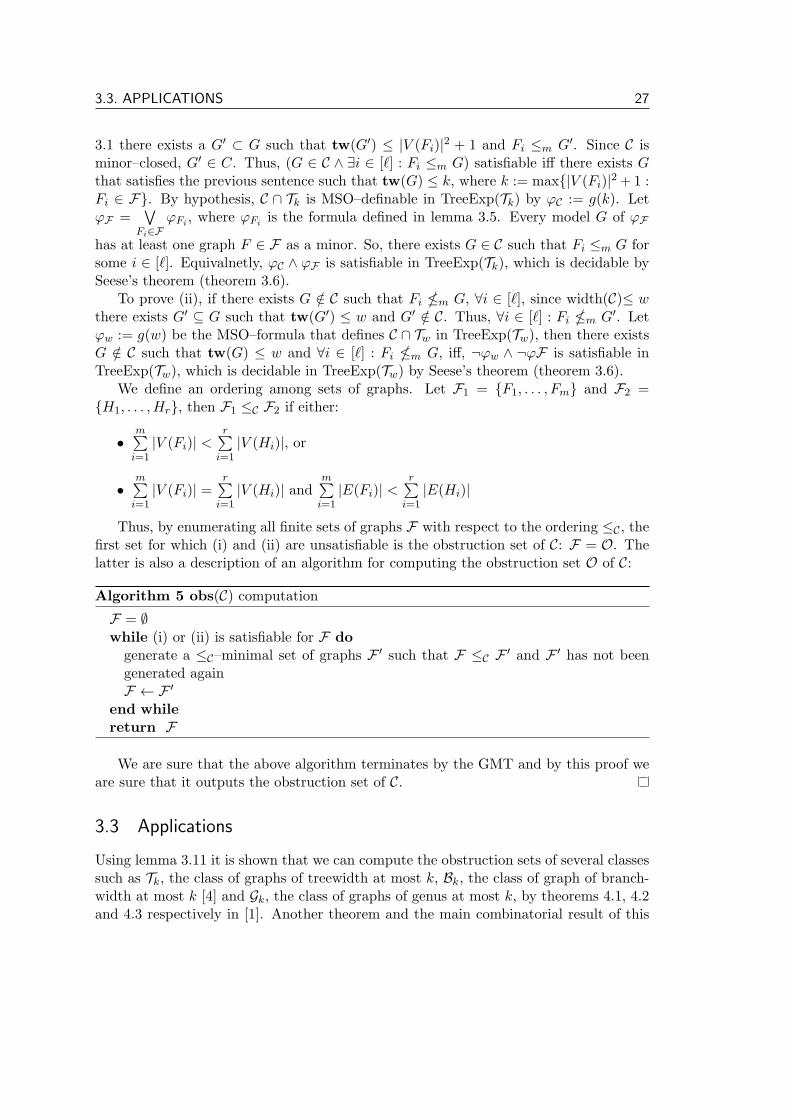
Thus, by enumerating all finite sets of graphs F with respect to the ordering ≤C , thefirst set for which (i) and (ii) are unsatisfiable is the obstruction set of C: F = O. Thelatter is also a description of an algorithm for computing the obstruction set O of C:

Algorithm 5 obs(C) computation

F = ∅while (i) or (ii) is satisfiable for F do

generate a ≤C–minimal set of graphs F ′ such that F ≤C F ′ and F ′ has not beengenerated againF ← F ′

end whilereturn F

We are sure that the above algorithm terminates by the GMT and by this proof weare sure that it outputs the obstruction set of C.

3.3 Applications

Using lemma 3.11 it is shown that we can compute the obstruction sets of several classessuch as Tk, the class of graphs of treewidth at most k, Bk, the class of graph of branch-width at most k [4] and Gk, the class of graphs of genus at most k, by theorems 4.1, 4.2and 4.3 respectively in [1]. Another theorem and the main combinatorial result of this

28 3. Trying MSO

paper is given in theorem 5.1 of the paper, which states that if we are given the obstruc-tion set of a minor–closed class C, then we can compute the obstruction set of Capex,where1 G ∈ Capex ⇐⇒ ∃v ∈ V (G) : G\v ∈ C. For proving the latter, Robertson andSeymour’s Trinity Lemma is essential, as well as the irrelevant vertex technique [26, 29]play a key role on proving that Capex has bounded width and since it is MSO–definable byφCapex . φCapex is the following formula: ∃v ∈ V ∃V ′∃E′(V ′ = V ∖ {v}∧E′ = {e ∈ E | v ∈

e ∩ V } ∧ ¬

( ∨Hi∈OC

φ′Hi

)), where OC is the obstruction set of C, φ′

Hi≡ ∃X1 . . . ∃Xkψ,

ψ ≡ [∧i =j

Xi ∩Xj = ∅ ∧∧i(∅ ⊆ Xi ⊆ V ′ ∧Xi is connencted )∧

∧{vi,vj}∈E(Hi)

∃xi ∈ Xi∃xj ∈

Xj∃z((xi, z) ∈ I(V ′, E′) ∧ (xj , z) ∈ I(V ′, E′))], I(V ′, E′) = {(v, e) : e ∈ E′ ∧ v ∈ e ∩ V ′}and vi are the vertices of Hi.

By applying the methods that where developed to prove that Capex has boundedwidth, the authors prove that if we are given the obstruction sets O1 and O2 of twominor–closed graph classes C1 and C2 respectively, then C1 ∪ C2 has bounded width and

since C1 ∪ C2 is MSO–definable by the formula ¬

( ∨H∈O1

φH

)∨ ¬

( ∨G∈O2

φG

)we can

apply lemma 3.11 and prove that OC1∪C2 is computable. This solves the union problem,and answers an open question from [6].

As a final remark, it is easy to see that for applying lemma 3.11, usually the easytask is to prove MSO–definability. The hard task is to prove that the class in studyhas bounded width, which we can easily understand by the use of the complex combi-natorial results that were employed to show that Capex has bounded width and to applythis methods to show that C1 ∪ C2 has also bounded width (given O and, O1 and O2

respectively). However, lemma 3.11 can be adapted to other well–quasi orderings. Inthe next chapter we will show that the methods of [1] that were presented in this chaptercan be adapted to immersion–closed graph classes and by combining them with someother combinatorial results we can also solve the union problem for immersion–closedgraph classes.

1We remind for this definition that G\v = (V ∖ {v}, E′), where E′ = {e ∈ E | v /∈ e ∩ V }.

Chapter 4

Immersion obstructions

In [1], I. Adler, M. Grohe and S. Kreutzer provide tools that allow us to use Seese’stheorem (theorem 3.6), when an upper bound on the tree-width of the obstructions isknown and an MSO–description of the graph class can be computed, in order to computethe obstruction sets of minor-closed graph classes. In this chapter we show how wecan adapt their machinery to the immersion relation and prove that the treewidth ofthe obstructions of immersion–closed graph classes is upper bounded by some functionthat only depends on the graph class. This provides a generic technique to constructimmersion obstruction sets when the explicit value of the function is known. Then, byobtaining such an explicit upper bound on the tree-width of the graphs in obs≤im(C),where C = C1 ∪ C2 and C1, C2 are immersion-closed graph classes whose obstruction setsare given, we show that the set obs≤im(C) can be effectively computed. These resultsappeared in [17].

4.1 Preliminaries

We firstly recall and give some basic definitions. We say that H is an immersion of G(or H is immersed in G), H ≤im G, if H can be obtained from a subgraph of G aftera (possibly empty) sequence of edge lifts, where the lift of two edges e1 = {x, y} ande2 = {x, z} to an edge e is the operation of removing e1 and e2 from G and then addingthe edge e = {y, z} in the resulting graph. Equivalently, we say that H is an immersionof G if there is an injective mapping f : V (H)→ V (G) such that, for every edge {u, v}of H, there is a path from f(u) to f(v) in G and for any two distinct edges of H thecorresponding paths in G are edge-disjoint, that is, they do not share common edges.

Additionally, if these paths are internally disjoint from f(V (H)), then we say thatH is strongly immersed in G. As above, the function f is called a model of H in G anda model with minimal number of vertices and edges is called minimal model. A graphclass C is called immersion–closed, if for every G ∈ C and every H with H ≤im G itholds that H ∈ C. For example, the class of graphs Et that admit a proper edge–coloringof at most t colors such that for every two edges of the same color every path betweenthem contains an edge of greater color is immersion–closed. (See [3]). Two paths are

29

30 4. Immersion obstructions

called vertex-disjoint if they do not share common vertices.

We will employ the ordering defined in the proof of lemma 3.11. The ordering ≤ isdefined between finite sets of graphs as follows: F1 ≤ F2 if and only if,

1.∑G∈F1

|V (G)| <∑H∈F2

|V (H)| or

2.∑G∈F1

|V (G)| =∑H∈F2

|V (H)| and∑G∈F1

|E(G)| <∑H∈F2

|E(H)|.

Definition 4.1. Let C be an immersion-closed graph class. A set of graphs F ={H1, . . . ,Hn} is called (immersion) obstruction set of C, and is denoted by obs≤im(C),if and only if F is a ≤-minimal set of graphs for which the following holds: For everygraph G, G does not belong to C if and only if there exists a graph H ∈ F such thatH ≤im G.

Recall (theorem 1.3) that by Robertson and Seymour’s fundamental result in [30],the obstruction set of every immersion–closed graph class is finite.

Let r be a positive integer. An r-approximate linkage in a graph G is a family L ofpaths in G such that for every r + 1 distinct paths P1, P2, . . . , Pr+1 in L, it holds that∩

i∈[r+1] V (Pi) = ∅ and each endpoint of the paths appears in exactly one path of L. Wecall these paths the components of the linkage. Let (α1, α2, . . . , αk) and (β1, β2, . . . , βk)be elements of V (G)k. We say that an r-approximate linkage L, consisting of the pathsP1, P2, . . . , Pk, links (α1, α2, . . . , αk) and (β1, β2, . . . , βk) if Pi is a path with endpointsαi and βi, for every i ∈ [k]. The order of such linkage is k. We call an r-approximatelinkage of order k, r-approximate k-linkage. Two r-approximate k-linkages L and L′ areequivalent if they have the same order and for every component P of L there exists acomponent P ′ of L′ with the same endpoints. An r-approximate linkage L of a graphG is called unique if for every equivalent linkage L′ of L, V (L) = V (L′). When r = 1,such a family of paths is called linkage. Finally, a linkage L in a graph G is called vitalif there is no other linkage in G joining the same pairs of vertices.

In [28], N. Robertson and P. Seymour proved a theorem which is known as The VitalLinkage Theorem. This theorem provides an upper bound for the tree-width of a graphG that contains a vital k-linkage L such that V (L) = V (G), where the bound dependsonly on k. A stronger statement of the Vital Linkage Theorem was recently provedby K. Kawarabayashi and P. Wollan [20], where instead of asking for the linkage to bevital, it asks for it to be unique. Notice here that a vital linkage is also unique. As insome of our proofs (for example, the proof of Lemma 4.14) we deal with unique but notnecessarily vital linkages we make use of the Vital Linkage Theorem in its latter formwhich is stated below.

Theorem 4.2 (The Unique Linkage Theorem[28, 20]). There exists a computable func-tion w : N → N such that the following holds. Let L be a (1-approximate) k-linkage inG with V (L) = V (G). If L is unique then tw(G) ≤ w(k).

4.2. COMPUTING IMMERSION OBSTRUCTION SETS 31

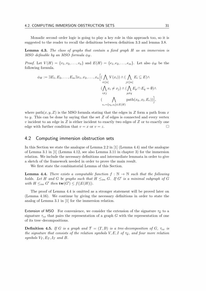
Monadic second–order logic is going to play a key role in this approach too, so it issuggested to the reader to recall the definitions between definition 3.3 and lemma 3.8.

Lemma 4.3. The class of graphs that contain a fixed graph H as an immersion isMSO–definable by an MSO–formula ϕH .

Proof. Let V (H) = {v1, v2, . . . , vn} and E(H) = {e1, e2, . . . , em}. Let also ϕH be thefollowing formula.

ϕH := ∃E1, E2, . . . , Em∃x1, x2, . . . , xn[(∧i∈[n]

V (xi)) ∧ (∧

j∈[m]

Ei ⊆ E)∧

(∧i=j

xi = xj) ∧ (∧p=q

Ep ∩ Eq = ∅)∧

(∧

er={vk,vl}∈E(H)

path(xk, xl, Er))],

where path(x, y, Z) is the MSO formula stating that the edges in Z form a path from xto y. This can be done by saying that the set Z of edges is connected and every vertexv incident to an edge in Z is either incident to exactly two edges of Z or to exactly oneedge with further condition that v = x or v = z.

4.2 Computing immersion obstruction sets

In this Section we state the analogue of Lemma 2.2 in [1] (Lemma 4.4) and the analogueof Lemma 3.1 in [1] (Lemma 4.12, see also Lemma 3.11 in chapter 3) for the immersionrelation. We include the necessary definitions and intermediate lemmata in order to givea sketch of the framework needed in order to prove the main result.

We first state the combinatorial Lemma of this Section.

Lemma 4.4. There exists a computable function f : N → N such that the followingholds. Let H and G be graphs such that H ≤im G. If G′ is a minimal subgraph of Gwith H ≤im G′ then tw(G′) ≤ f(|E(H)|).

The proof of Lemma 4.4 is omitted as a stronger statement will be proved later on(Lemma 4.16). We continue by giving the necessary definitions in order to state theanalog of Lemma 3.1 in [1] for the immersion relation.

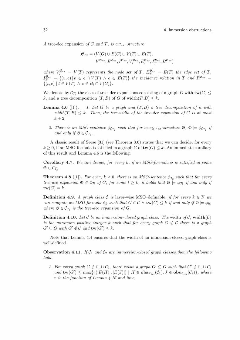
Extension of MSO For convenience, we consider the extension of the signature τG to asignature τex that pairs the representation of a graph G with the representation of oneof its tree–decompositions.

Definition 4.5. If G is a graph and T = (T,B) is a tree-decomposition of G, τex isthe signature that consists of the relation symbols V,E, I of τG, and four more relationsymbols VT , ET , IT and B.


A tree-dec expansion of G and T , is a τex–structure

Gex = (V (G) ∪ E(G) ∪ V (T ) ∪ E(T ),

V Gex , EGex , IGex , V GexT , EGex

T , IGexT , BGex)

where V GexT = V (T ) represents the node set of T , EGex

T = E(T ) the edge set of T ,

IGexT = {(v, e) | v ∈ e ∩ V (T ) ∧ e ∈ E(T )} the incidence relation in T and BGex ={(t, v) | t ∈ V (T ) ∧ v ∈ Bt ∩ V (G)}.

We denote by CTk the class of tree–dec expansions consisting of a graph G with tw(G) ≤k, and a tree decomposition (T,B) of G of width(T,B) ≤ k.

Lemma 4.6 ([1]). 1. Let G be a graph and (T,B) a tree decomposition of it withwidth(T,B) ≤ k. Then, the tree-width of the tree-dec expansion of G is at mostk + 2.

2. There is an MSO-sentence ϕCTk such that for every τex-structure G, G |= ϕCTk ifand only if G ∈ CTk .

A classic result of Seese [31] (see Theorem 3.6) states that we can decide, for everyk ≥ 0, if an MSO-formula is satisfied in a graph G of tw(G) ≤ k. An immediate corollaryof this result and Lemma 4.6 is the following.

Corollary 4.7. We can decide, for every k, if an MSO-formula ϕ is satisfied in someG ∈ CTk .

Theorem 4.8 ([1]). For every k ≥ 0, there is an MSO-sentence ϕTk such that for everytree-dec expansion G ∈ CTl of G, for some l ≥ k, it holds that G |= ϕTk if and only iftw(G) = k.

Definition 4.9. A graph class C is layer-wise MSO–definable, if for every k ∈ N wecan compute an MSO-formula ϕk such that G ∈ C ∧ tw(G) ≤ k if and only if G |= ϕk,where G ∈ CTk is the tree-dec expansion of G.

Definition 4.10. Let C be an immersion–closed graph class. The width of C, width(C)is the minimum positive integer k such that for every graph G /∈ C there is a graphG′ ⊆ G with G′ /∈ C and tw(G′) ≤ k.

Note that Lemma 4.4 ensures that the width of an immersion-closed graph class iswell-defined.

Observation 4.11. If C1 and C2 are immersion-closed graph classes then the followinghold.

1. For every graph G /∈ C1 ∪ C2, there exists a graph G′ ⊆ G such that G′ /∈ C1 ∪ C2and tw(G′) ≤ max{r(|E(H)|, |E(J)|) | H ∈ obs≤im(C1), J ∈ obs≤im(C2)}, wherer is the function of Lemma 4.16 and thus,

4.3. TREEWIDTH BOUNDS FOR THE OBSTRUCTIONS 33

2. For every graph G /∈ C1, there exists a graph G′ ⊆ G such that G′ /∈ C1and tw(G′) ≤ max{f(|E(H)|) | H ∈ obs≤im(C1)}, where f is the function ofLemma 4.4.

Finally, we state the analog of Lemma 3.1 in [1] for the immersion relation.

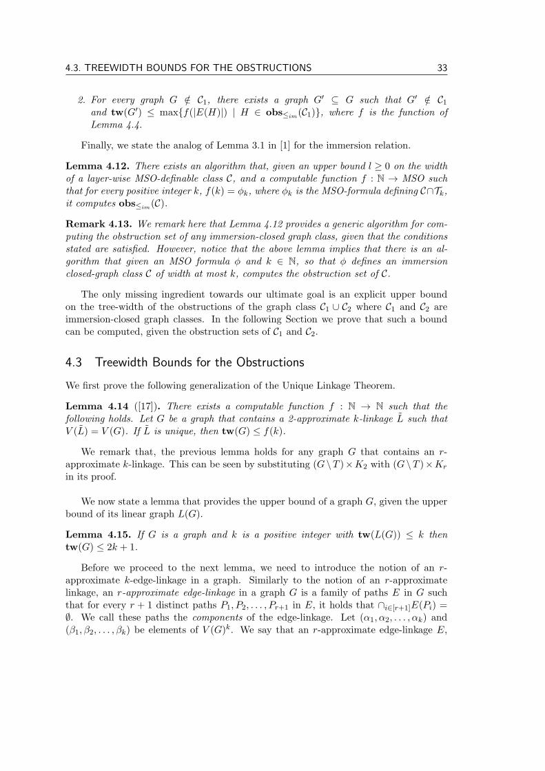
Lemma 4.12. There exists an algorithm that, given an upper bound l ≥ 0 on the widthof a layer-wise MSO-definable class C, and a computable function f : N → MSO suchthat for every positive integer k, f(k) = ϕk, where ϕk is the MSO-formula defining C∩Tk,it computes obs≤im(C).

Remark 4.13. We remark here that Lemma 4.12 provides a generic algorithm for com-puting the obstruction set of any immersion-closed graph class, given that the conditionsstated are satisfied. However, notice that the above lemma implies that there is an al-gorithm that given an MSO formula ϕ and k ∈ N, so that ϕ defines an immersionclosed-graph class C of width at most k, computes the obstruction set of C.

The only missing ingredient towards our ultimate goal is an explicit upper boundon the tree-width of the obstructions of the graph class C1 ∪ C2 where C1 and C2 areimmersion-closed graph classes. In the following Section we prove that such a boundcan be computed, given the obstruction sets of C1 and C2.

4.3 Treewidth Bounds for the Obstructions

We first prove the following generalization of the Unique Linkage Theorem.

Lemma 4.14 ([17]). There exists a computable function f : N → N such that thefollowing holds. Let G be a graph that contains a 2-approximate k-linkage L such thatV (L) = V (G). If L is unique, then tw(G) ≤ f(k).

We remark that, the previous lemma holds for any graph G that contains an r-approximate k-linkage. This can be seen by substituting (G \T )×K2 with (G \T )×Kr

in its proof.

We now state a lemma that provides the upper bound of a graph G, given the upperbound of its linear graph L(G).

Lemma 4.15. If G is a graph and k is a positive integer with tw(L(G)) ≤ k thentw(G) ≤ 2k + 1.

Before we proceed to the next lemma, we need to introduce the notion of an r-approximate k-edge-linkage in a graph. Similarly to the notion of an r-approximatelinkage, an r-approximate edge-linkage in a graph G is a family of paths E in G suchthat for every r + 1 distinct paths P1, P2, . . . , Pr+1 in E, it holds that ∩i∈[r+1]E(Pi) =∅. We call these paths the components of the edge-linkage. Let (α1, α2, . . . , αk) and(β1, β2, . . . , βk) be elements of V (G)k. We say that an r-approximate edge-linkage E,


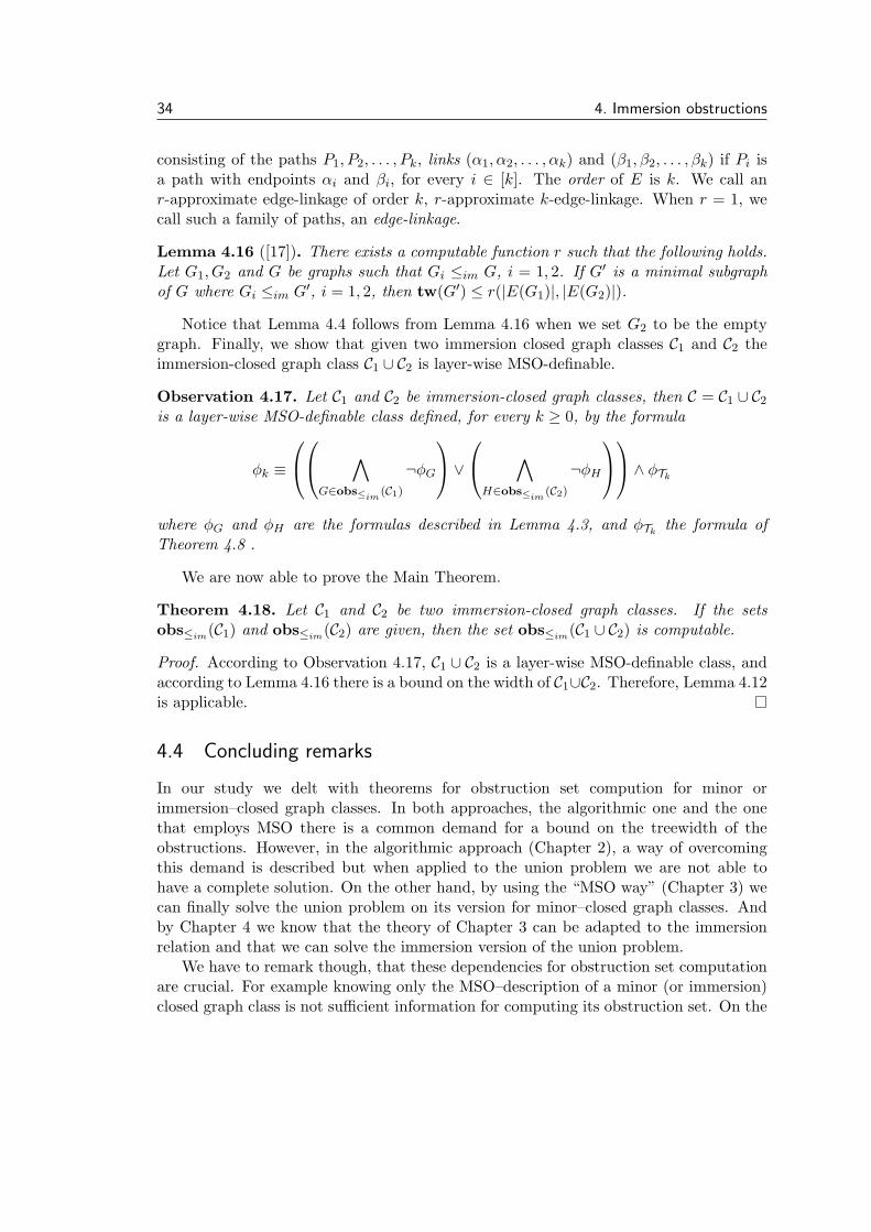
consisting of the paths P1, P2, . . . , Pk, links (α1, α2, . . . , αk) and (β1, β2, . . . , βk) if Pi isa path with endpoints αi and βi, for every i ∈ [k]. The order of E is k. We call anr-approximate edge-linkage of order k, r-approximate k-edge-linkage. When r = 1, wecall such a family of paths, an edge-linkage.

Lemma 4.16 ([17]). There exists a computable function r such that the following holds.Let G1, G2 and G be graphs such that Gi ≤im G, i = 1, 2. If G′ is a minimal subgraphof G where Gi ≤im G′, i = 1, 2, then tw(G′) ≤ r(|E(G1)|, |E(G2)|).

Notice that Lemma 4.4 follows from Lemma 4.16 when we set G2 to be the emptygraph. Finally, we show that given two immersion closed graph classes C1 and C2 theimmersion-closed graph class C1 ∪ C2 is layer-wise MSO-definable.

Observation 4.17. Let C1 and C2 be immersion-closed graph classes, then C = C1 ∪ C2is a layer-wise MSO-definable class defined, for every k ≥ 0, by the formula

ϕk ≡

∧G∈obs≤im

(C1)

¬ϕG

∨ ∧

H∈obs≤im(C2)

¬ϕH

∧ ϕTkwhere ϕG and ϕH are the formulas described in Lemma 4.3, and ϕTk the formula ofTheorem 4.8 .

We are now able to prove the Main Theorem.

Theorem 4.18. Let C1 and C2 be two immersion-closed graph classes. If the setsobs≤im(C1) and obs≤im(C2) are given, then the set obs≤im(C1 ∪ C2) is computable.

Proof. According to Observation 4.17, C1 ∪ C2 is a layer-wise MSO-definable class, andaccording to Lemma 4.16 there is a bound on the width of C1∪C2. Therefore, Lemma 4.12is applicable.

4.4 Concluding remarks

In our study we delt with theorems for obstruction set compution for minor orimmersion–closed graph classes. In both approaches, the algorithmic one and the onethat employs MSO there is a common demand for a bound on the treewidth of theobstructions. However, in the algorithmic approach (Chapter 2), a way of overcomingthis demand is described but when applied to the union problem we are not able tohave a complete solution. On the other hand, by using the “MSO way” (Chapter 3) wecan finally solve the union problem on its version for minor–closed graph classes. Andby Chapter 4 we know that the theory of Chapter 3 can be adapted to the immersionrelation and that we can solve the immersion version of the union problem.

We have to remark though, that these dependencies for obstruction set computationare crucial. For example knowing only the MSO–description of a minor (or immersion)closed graph class is not sufficient information for computing its obstruction set. On the

4.4. CONCLUDING REMARKS 35

other hand, there is a need for a bound on the treewidth of the obstructions in both ofthe approaches studied and we do not know a generic procedure to compute one.

Finally, we are only concerned with matters of computability in our study, but allof our algorithms for obstruction set computation enumerate either graphs or sets ofgraphs, which is a rather “expensive” procedure in matters of time complexity. Sincethe aspect of computability is well studied, a direction for further research could involveways to improve the time complexity of these algorithms or even new approaches thatrequire less computational time. However, the obstruction sets are usually large sets.For example, a super–exponential lower bound on the size of the obstruction set fora certain family of graph classes is proven in [18] (see Theorem 1.7) which implies asuper–exponential bound on the running time of every algorithm that computes it: onlyfor “writing” an output of size n we need n amount of time.

Bibliography

[1] I. Adler, M. Grohe, S. Kreutzer, Computing Excluded Minors. S.-H.-Teng (Ed.),SODA. SIAM. pp. 641-650, 2008.

[2] S. Arnborg and A. Proskurowski. Linear time algorithms for NP-hard problemsrestricted to partial k-trees. Discrete Appl. Math. 23:1124, 1989.

[3] H. L. Bodlaender, J. S. Deogun, K. Jansen, T. Kloks, D. Kratsch, H. Muller, andZ. Tuza. Rankings of graphs. SIAM J. Discrete Math., 11(1):168–181 (electronic),1998.

[4] H.L. Bodlaender, D.M. Thilikos. Treewidth for graphs with small chordality. Dis-crete Applied Mathematics, Vol. 79, No. 1-3, pp. 45–61, 1997.

[5] H. L. Bodlaender. A partial k–arboretum of graphs with bounded treewidth. The-oretical Computer Science 209 (12): 145, 1998.

[6] K. Cattell, M. Dinneen, R. Downey, M. R. Fellows, M. Langston. On computinggraph minor obstruction sets. Theoretical Computer Science 233, 107-127, 2000.

[7] K. Cattell, M. J. Dinneen and M. R. Fellows. A simple linear time algorithm forfinding path decompositions of small width. Information Processing Letters 57 ,197–203, 1996.

[8] K. Cattell, M. J. Dinneen and M. R. Fellows. Obstructions to within a few ver-tices or edges of acyclic.Proceedings WADS ’95, Springer–Verlag, Lecture Notes inComputer Science vol. 995, 415–427, 1995.

[9] K. Cattell and M. J. Dinneen. A characterization of graphs with vertex cover up tofive. Proceedings ORDAL ’94, Springer–Verlag, Lecture Notes in Computer Sciencevol. 831, 86–99, 1994.

[10] B. Courcelle, R. G. Downey, and M. R. Fellows. A note on the computability ofgraph minor obstruction sets for monadic second order ideals. Journal of UniversalComputer Science, 3:11941198, 1997.

[11] B. Courcelle and J. Lagergren. Equivalent definitions of recognizability for graphsof bounded tree-width. Mathematical Structure in Computer Science, to appear.

37

38 BIBLIOGRAPHY

[12] R. Diestel. Graph Theory. Graduate Texts in Mathematics, Spirnger–Verlag, 4th

edition, 2010.

[13] H. B. Enderton. A Mathematical Introduction to Logic. Academic Press, New York,1972.

[14] J. Erickson. Computational Topology. Class notes, Department of Computer Sci-ence, University of Illinois, Urbana–Champaign.http://compgeom.cs.uiuc.edu/~jeffe/teaching/comptop/

[15] M. R. Fellows and M. A. Langston. An analogue of the Myhill–Nerode theoremand its use in computing finite–basis characterizations. Proc. Symposium on theFoundations of Computer Science (FOCS), IEEE Press, 520–525, 1989.

[16] M. R. Fellows and M. A. Langston. On search, decision and the efficiency of poly-nomial time algorithms. Proc. Symposium on the Theory of Computing (STOC),ACM Press, 501–512, 1989.

[17] A. Giannopoulou, I. Salem, D. Zoros. Effective Computation of Immersion Obstruc-tions for Unions of Graph Classes. 13th Scandinavian Symposium and Workshopson Algorithm Theory, 2012.

[18] A. Giannopoulou, D. M. Thilikos. Obstructions for Tree–depth. Electronic notes inDiscrete Mathematics 34, 249–253, 2009.

[19] J. Hopcroft and R.E. Tarjan. Efficient planarity testing. Journal of the Associationfor Computing Machinery 21 (4): 549–568, 1974.

[20] K. Kawarabayashi and P. Wollan. A shorter proof of the graph minor algorithm:the unique linkage theorem. In Leonard J. Schulman, editor, STOC, pages 687–694.ACM, 2010.

[21] W. Kocay. The Hopcroft–Tarjan Planarity Algorithm. Unpublished.http://www.combinatorialmath.ca/G&G/articles/planarity.pdf

[22] J. B. Kruskal. Well–quasi–ordering, the Tree Theorem, and Vazsonyps conjecture.Trans. Amer. Math. Soc. 95, pp. 210225, 1960.

[23] L. Lovasz. Graph Minor Theory. Bulletin (New Series) of the American Mathemat-ical Society. Volume 43, number 1, pages 75–86, 2005.

[24] E. Mendelson. Introduction to Mathematical Logic. 2nd ed. Van Nostrand–Reinhold,New York, 1978.

[25] N. Robertson and P. D. Seymour, Graph minors. II. Algorithmic aspects of tree-width. J. Algorithms 7(3):309322, 1986.

[26] N. Robertson and P. D. Seymour, Graph minors XIII. The disjoint paths problem.Journal of Combinatorial Theory, Series B, 63:65110, 1995.

http://compgeom.cs.uiuc.edu/~jeffe/teaching/comptop/

http://www.combinatorialmath.ca/G&G/articles/planarity.pdf

BIBLIOGRAPHY 39

[27] N. Robertson and P. D. Seymour, Graph minors XX. Wagners conjecture. Journalof Combinatorial Theory, Series B, 92:325357, 2004.

[28] N. Robertson and P. D. Seymour. Graph minors XXI. Graphs with unique linkages.J. Comb. Theory, Ser. B, 99(3):583–616, 2009.

[29] N. Robertson and P. D.Seymour. Graph minors XII. Irrelevant vertices in linkageproblems. submitted for publication, 2006.http://www.math.princeton.edu/~pds/papers/GM22/GM22.pdf

[30] N. Robertson and P. D. Seymour. Graph minors XXIII. Nash–Williams’ immersionconjecture, Journal of Combinatorial Theory, Series B 100 (2): 181205, 2010.

[31] D. Seese. The structure of models of decidable monadic theories of graphs. Annalsof Pure and Applied Logic, 53:169195, 1991.

http://www.math.princeton.edu/~pds/papers/GM22/GM22.pdf

Iosif Salem - Εθνικόν και Καποδιστριακόν...

Documents

Transcript of Iosif Salem - Εθνικόν και Καποδιστριακόν...