Smart Grid and Renewable Energy, 2016, 7, 16-45 Published Online January 2016 in SciRes. http://www.scirp.org/journal/sgre http://dx.doi.org/10.4236/sgre.2016.71002

How to cite this paper: Mahmoud, G.A. and Oda, E.S.S. (2016) Investigation of Connecting Wind Turbine to Radial Distribu-tion System on Voltage Stability Using SI Index and λ-V Curves. Smart Grid and Renewable Energy, 7, 16-45. http://dx.doi.org/10.4236/sgre.2016.71002

Investigation of Connecting Wind Turbine to Radial Distribution System on Voltage Stability Using SI Index and λ-V Curves Gamal Abd El-Azeem Mahmoud, Eyad Saeed Soliman Oda Department of Electrical Engineering, Faculty of Engineering, Suez Canal University, Ismailia, Egypt

Received 27 November 2015; accepted 25 January 2016; published 28 January 2016

Copyright © 2016 by authors and Scientific Research Publishing Inc. This work is licensed under the Creative Commons Attribution International License (CC BY). http://creativecommons.org/licenses/by/4.0/

Abstract The growth of wind energy penetration level in distribution system raises the concern about its impact on the operation of the power system, especially voltage stability and power loss. Among the major concerns, this paper studied the impact of connecting wind Turbine (WT) in radial dis-tribution system with different penetration levels and different power factor (lead and lag) on power system voltage stability and power loss reduction. Load flow calculation was carried out using forward-backward sweep method. The analysis proceeds on 9- and 33-bus radial distribu-tion systems. Results show that voltage stability enhancement and power loss reduction should be considered as WT installation objective.

Keywords Power Loss, Radial Distribution System, Si Index, Voltage Stability, Optimal Size and Location of Wind Turbine

1. Introduction In the past few years, great progress has been achieved in wind energy (WE) field as distributed generation source (DGS) because wind energy has a lot of merits such as environment, economic and technical. Environ-mentally it’s clean energy source and meets the requirement of reducing global warming. Technically the single wind turbine capable of generating power in few MW at present and in near future 2020 the rated power of WT may reach 10 - 20 MW [1]. Economically it’s the cheapest renewable energy source [1] [2], these merits make wind energy the most suitable source for future energy. Therefore, the penetration of wind turbines in electrical power systems will increase and they may begin to influence overall power system behavior, making it impossible

G. A. Mahmoud, E. S. S. Oda

17

to run a power system by only controlling large scale power plants. So it is important to study the behavior of wind turbines in an electrical power system. Refs [3]-[6] were concerned in impact of connecting distributed generation (DG) to the grid on voltage stability, to study the optimal penetration level of wind farms without compromising the system voltage stability in transmission level using energy storage systems studied in ref [7], while ref. [8] presented the impact of fixed speed WT on grid voltage stability in transmission level.

Distribution system (DS) is an important part of power system, and it represents the link between the bulk system and customers. It is estimated that as much as 13% of the total power generation is lost in the distribution networks. Approximately 70% of the total electric power system real power losses are associated with the dis-tribution level [9]. Wind energy farms usually located at distribution area, so it’s essential to study the behavior associated with connecting wind turbine generation units to distribution level.

Voltage stability and power losses problems are annoying problems in DS, voltage stability may spread to transmission system and cause blackout for the whole system. Extensive studies are needed to determine the best connection of WT to DSs with acceptable voltage level.

This paper is organized as follows. Section 2 describes load flow in distribution system. Section 3 describes the wind turbine penetration level. Section 4 describes the voltage stability index used to study voltage stability margin of the system. Section 5 describes power loss reduction. Section 6 describes optimization technique used to choose optimal size and location of WT. Results obtained considering voltage stability margin, voltage profile, and power loss are presented in Sections 7 and 8. Finally, Section 9 summarizes the main conclusions.

2. Distribution System and Load Flow Power flow problems can be solved by several methods and are classified as either direct or iterative. The direct methods employ the direct solutions related to the linear system, but actually all methods are iterative because the basic problem involves the solution of a system of non-linear equations.

Although conventional power flow methods such as Newton-Raphson (NR) technique, Fast decoupled (FD) load flow and Gauss-Seidel are well developed in dealing with the transmission and sub-transmission sections of the power system networks, they are considered to be inefficient in handling distribution networks. This is be-cause the (DS) is different in several ways from its transmission counterpart. DS has a strictly radial topology nature or weakly meshed networks in contrast with transmission sys-

tems which are “tightly” meshed networks. DS is a low voltage system having low X/R ratio sections and a wide range of reactance and resistance

values. The practical DSs low X/R ratio sections may cause both the NR and FD conventional methods to di-verge. The line impedance angles are small enough to deteriorate the dominance of the NR Jacobian main di-agonal, making it prone to singularity. Such a low X/R value would also prevent the Jacobian matrix from being decoupled and simplified. DS may consist of a tremendously large number of sections and buses spread throughout the network. All of these characteristics strongly suggest that DS is to be classified as an ill-conditioned power system. In this paper a popular solution method used to treat ill conditioning is the forward-backward sweep (FB)

method. The forward/backward method has been developed by D. Thukaram [10]; this method employs Ohm’s law, Kirchhoff Voltage Law and Kirchhoff Current Law to calculate nodal voltages and branch currents.

The backward stage determines the branch currents from the end node towards the root node with a constant nodal voltage, while the forward stage is used to determine the nodal voltages by assuming the source nodal voltage is constant. The forward-backward substitution was replaced by the forward-backward sweep technique. The technique used in this paper is proposed in appendix A for more details refer to ref [11].

3. Wind Turbine Penetration Level Wind turbine Penetration Level (PL) used to study its impact on the power system operation. This PL gives per-centage WT generated power contribution in load supply is given by:

100WT

l

PPLP

= × (1)

where

G. A. Mahmoud, E. S. S. Oda

18

PWT: wind turbine active power. Pl: total loadsactive power. The paper studied the impact of WT at different PL and different power factor (p.f) i.e. (lead and lag) on dis-

tribution system operation.

4. Voltage Stability The voltage instability problem in a distribution network may spread to the transmission network causing a blackout as happened in Brazilian system in June 1997 [12], US/Canada blackout, the Scandinavian blackout and the Italian blackout, which all happened in 2003 [13]. It is attracting more attention from researchers around the world.

There are several definitions of voltage stability. One definition developed by IEEE and CIGRE that Voltage stability refers to the ability of a power system to maintain steady voltages at all buses in the system after being subjected to a disturbance from a given initial operating condition [14].

The term voltage collapse is also often used. It is the process by which the sequence of events accompanying voltage instability leads to a blackout or abnormally low voltages in a significant part of the power system.

Voltage Stability Indices The main objective of Voltage Stability Indices (VSIs) is to estimate the distance from the current operating point to the system voltage marginally stable point. Numerical indices help operators to monitor how close the system is to collapse or to initiate automatic remedial action schemes to prevent voltage collapse.

Most of the VSIs that have been proposed are based on steady state power flow. An index, which can be evaluated at all buses in radial distribution systems, was presented by M. Charkra-

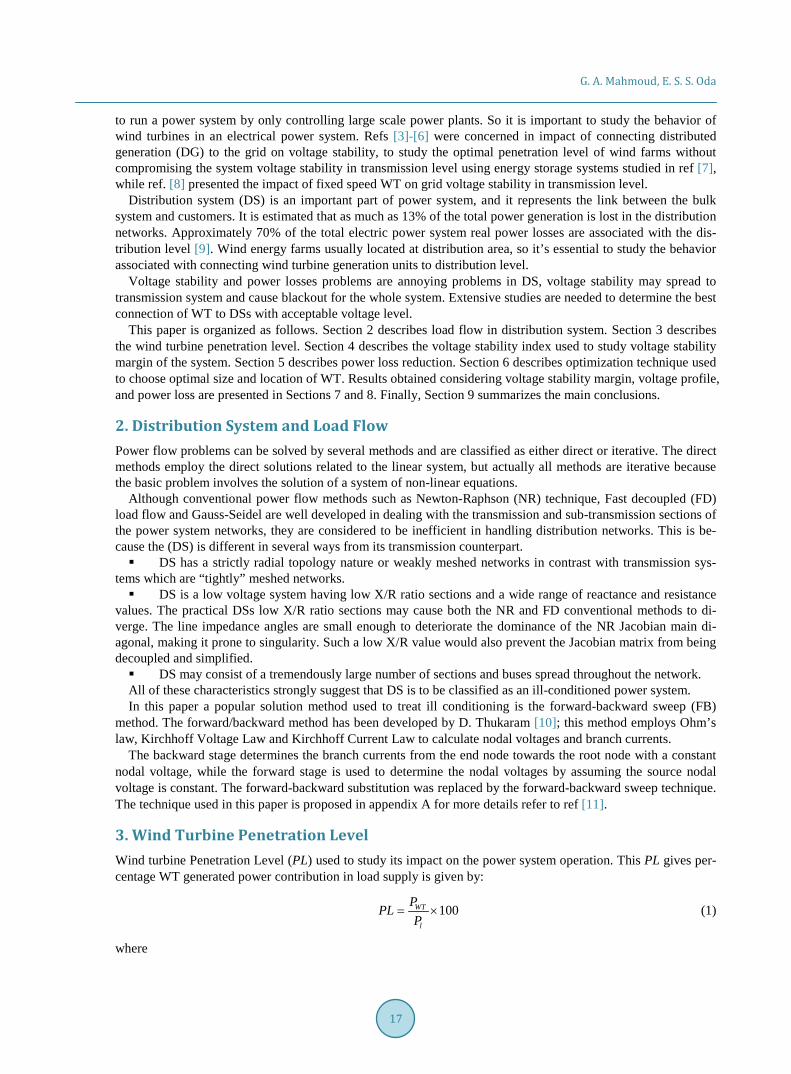
vorty and D. Das in [15]. The distribution system can be represented by the equivalent of two bus system as showing in Figure 1; the

Equation represents the voltage stability index SI is given by:

( ) ( ) ( ) ( ) ( ) ( )

( ) ( ) ( ) ( ) ( )

4 2

2

1 4.0 1 1

4.0 1 1

SI i V i P i x i Q i r i

P i r i Q i x i V i

+ = − + − +

− + + + (2)

where ( )1SI i + : Voltage stability index of bus i + 1 ( 1, 2, ,i n= ).

n: the total number of buses. i: the branch number. r (i): resistance of branch i. x (i): reactance of branch i. V (i): voltage of bus i. V (i + 1): voltage of bus i + 1. P (i + 1): total real power load fed through bus i + 1. Q (i + 1): total reactive power load fed through bus i + 1. When SI approaches 0.0, that means the system is unstable.

i i+1

Pi+1Qi+1

ri xi

Vi∟δi Vi+1∟δi+1

Sending EndReceving End

PWT

QWT

PiQi

Figure 1. Simple two bus system.

G. A. Mahmoud, E. S. S. Oda

19

5. Power Losses Before the WT connected to the system showing in Figure 1, the total active power losses are:

1

2 2

20 0

I

n ni i

loss ii i i

P QP r

V+= =

+= ×

∑ ∑ (3)

Once the WT is connected at the system, three different situations may take place:

• situation 1: ( ) ( ) 11

WTload ii

P P++

< ∑

• situation 2: ( ) ( ) 11

WTload ii

P P++

= ∑

• situation 3: ( ) ( ) 11

WTload ii

P P++

> ∑

For situations 1 and 2, the injection of PWT reduces the Pi drawn from bus i. In other words, the WT reduces the load’s value at bus i + 1. However, the WT in situation 3 acts as in situations 1 and 2, plus it will reverse a portion of the injected PWT back to bus i. Reducing the power loss and maintaining the voltage within acceptable limits are vital in WT applications. Although the first and second situations’ results in some cases are significant, situation 3 leads to better results if the optimal WT size and location are employed.

To evaluate the impact of installing WT at distribution feeder on power loss reduction (PLR) the following relation used:

% 100WT

LOSS LOSS

LOSS

P PPLR

P−

= × (4)

where PLOSS: System losses without WT

WTLOSSP : System loss after WT installation

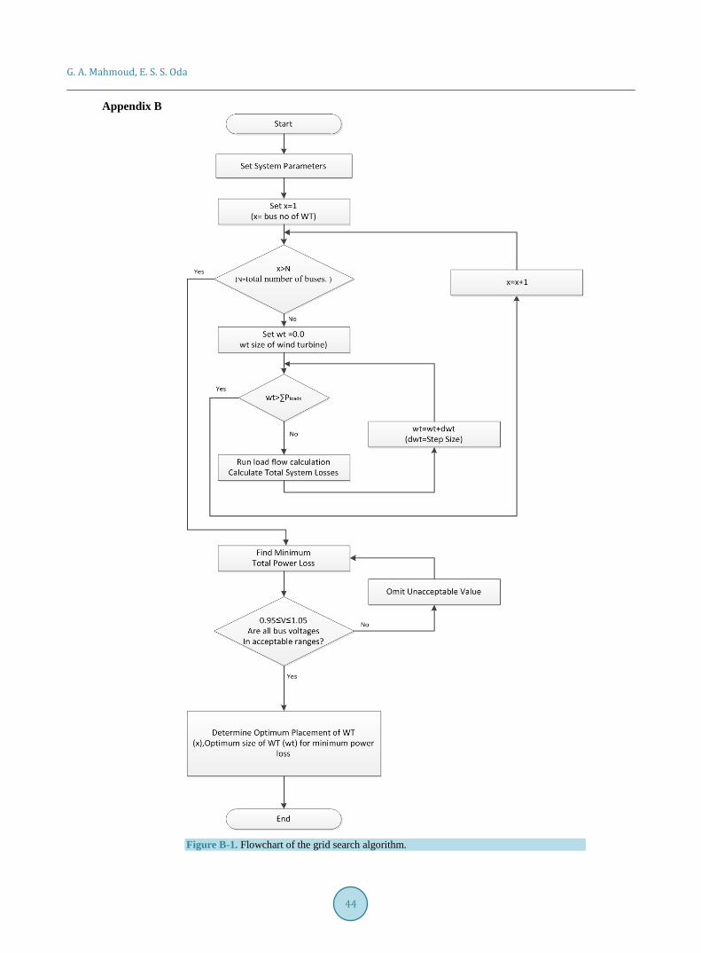
6. Optimal Size and Location of WT Optimal location and size of WT generation obtained using Grid Search Algorithm [16]-[18]. The Grid Search Algorithm is applied by adding WT to each bus, changing the size of WT from 0% of total load power to 100% of total load power with the step size of 0.05% of total load power. In this algorithm, the objective is to minim-ize total power losses of the system (PlossT) by injected active power of WT (PWT) for WT placement The main constraints are to restrict the voltages along the radial system within 1 ± 0.05 pu, as in Equation (5-a) and Equa-tion (5-b).

To minimize ( )WTlossTf P P= subject to

1 0.05 p.u 1,2, ,iV i n≤ ± = (5-a)

0 WTloadP P≤ ≤ ∑ (5-b)

The flowchart of the Grid Search algorithm to determine the optimum size and location of WT is proposed in the appendix B Figure B-1.

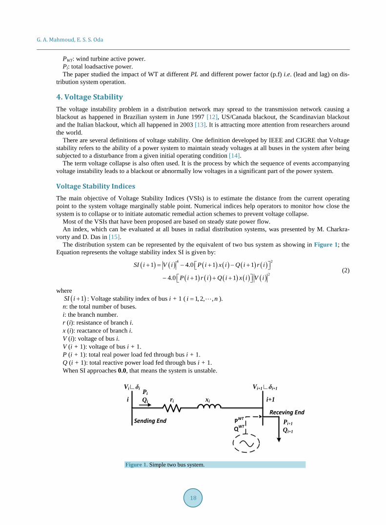
7. First Case Study The first test case is a 9-bus [11] [19], single feeder, radial distribution system shown in Figure 2. This system has no laterals. The rated line voltage of the system is 23 kV. The details of the feeder and the load characteris-tics are given in Table C-1 in Appendix C.

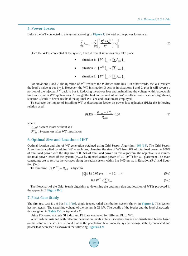
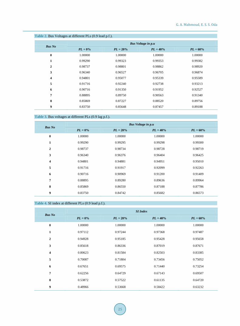
Using FB sweep analysis SI index and PLR are evaluated for different PL of WT. Wind turbine installed with different penetration levels at bus 9 (weakest branch of distribution feeder based

on the value of the VSI). It’s found that as the penetration level increase system voltage stability enhanced and power loss decreased as shown in the following Figures 3-9.

G. A. Mahmoud, E. S. S. Oda

20

Figure 2. Single line diagram of 9-bus feeder.

Figure 3. Bus voltages at different PLs (0.9 lead p.f.).

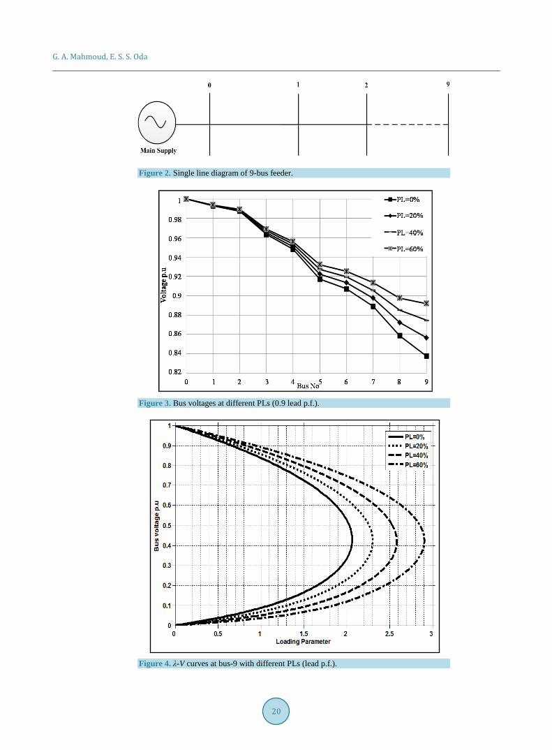
Figure 4. λ-V curves at bus-9 with different PLs (lead p.f.).

G. A. Mahmoud, E. S. S. Oda

21

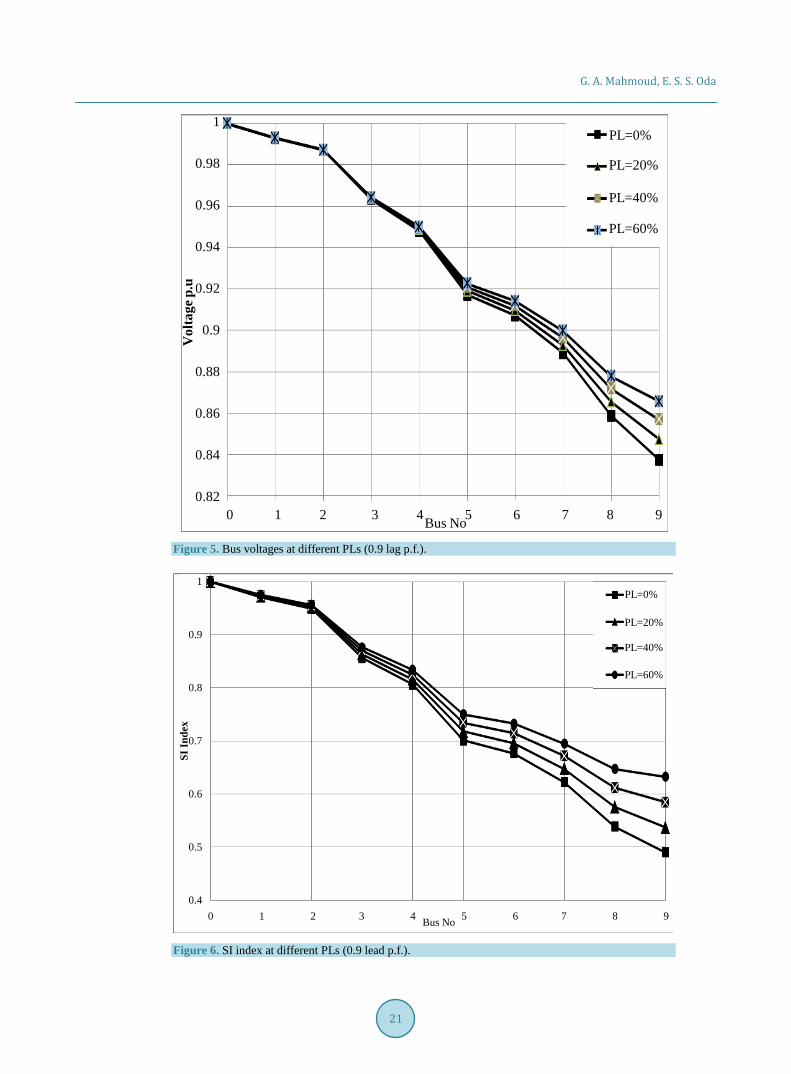
Figure 5. Bus voltages at different PLs (0.9 lag p.f.).

Figure 6. SI index at different PLs (0.9 lead p.f.).

Bus No

PL=0%

PL=40%

PL=60%

PL=20%

0 1 2 3 4 5 6 7 8 9

Vol

tage

p.u

1

0.98

0.96

0.94

0.92

0.9

0.88

0.86

0.84

0.82

PL=0%

PL=40%

PL=60%

PL=20%

Bus No0 1 2 3 4 5 6 7 8 9

1

0.9

0.8

0.7

0.6

0.5

0.4

SI In

dex

G. A. Mahmoud, E. S. S. Oda

22

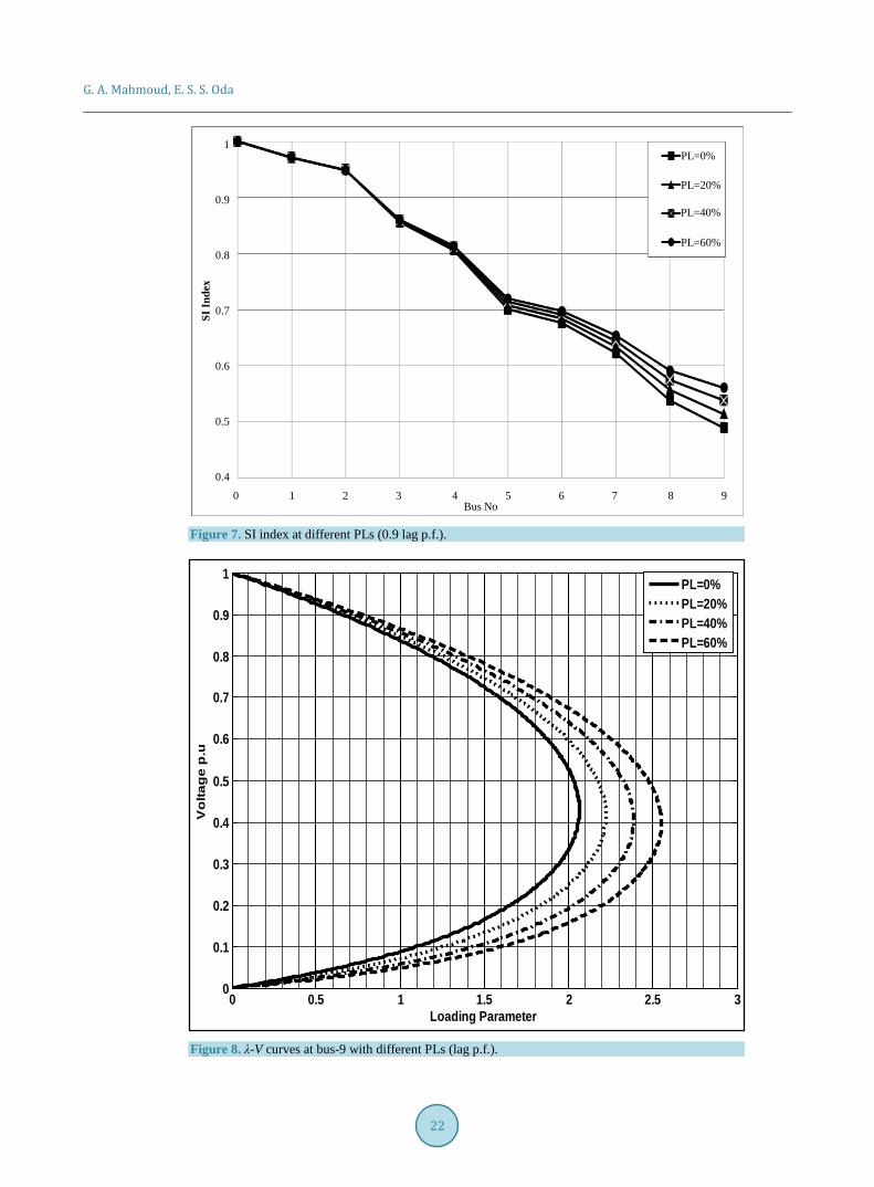
Figure 7. SI index at different PLs (0.9 lag p.f.).

Figure 8. λ-V curves at bus-9 with different PLs (lag p.f.).

PL=0%

PL=40%

PL=60%

PL=20%

SI In

dex

1

0.9

0.8

0.7

0.6

0.5

0.4

Bus No0 1 2 3 4 5 6 7 8 9

0 0.5 1 1.5 2 2.5 30

0.1

0.2

0.3

0.4

0.5

0.6

0.7

0.8

0.9

1

Loading Parameter

Vo

ltag

e p

.u

PL=0%PL=20%PL=40%PL=60%

G. A. Mahmoud, E. S. S. Oda

23

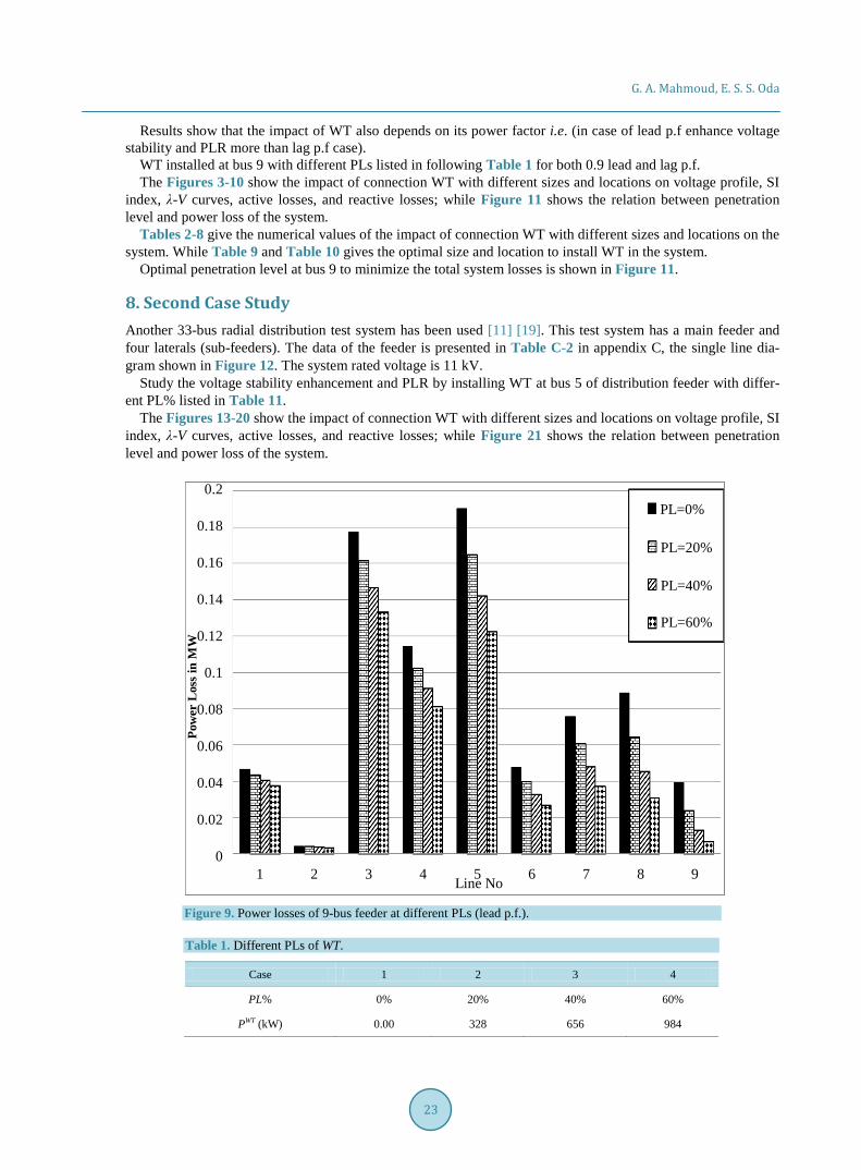
Results show that the impact of WT also depends on its power factor i.e. (in case of lead p.f enhance voltage stability and PLR more than lag p.f case).

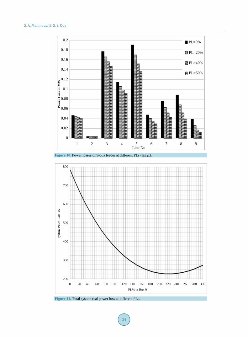
WT installed at bus 9 with different PLs listed in following Table 1 for both 0.9 lead and lag p.f. The Figures 3-10 show the impact of connection WT with different sizes and locations on voltage profile, SI

index, λ-V curves, active losses, and reactive losses; while Figure 11 shows the relation between penetration level and power loss of the system.

Tables 2-8 give the numerical values of the impact of connection WT with different sizes and locations on the system. While Table 9 and Table 10 gives the optimal size and location to install WT in the system.

Optimal penetration level at bus 9 to minimize the total system losses is shown in Figure 11.

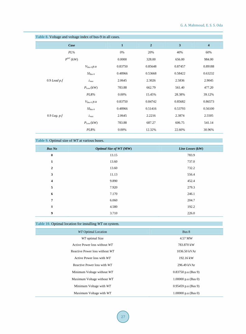
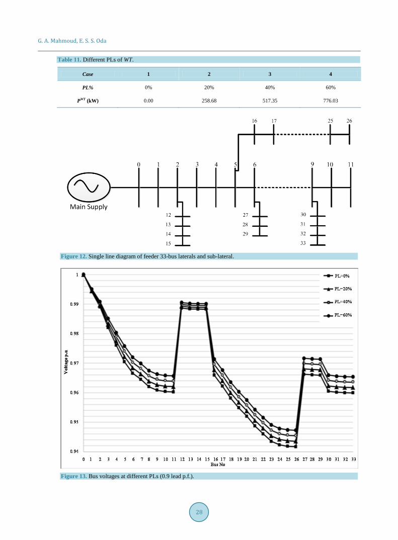
8. Second Case Study Another 33-bus radial distribution test system has been used [11] [19]. This test system has a main feeder and four laterals (sub-feeders). The data of the feeder is presented in Table C-2 in appendix C, the single line dia-gram shown in Figure 12. The system rated voltage is 11 kV.

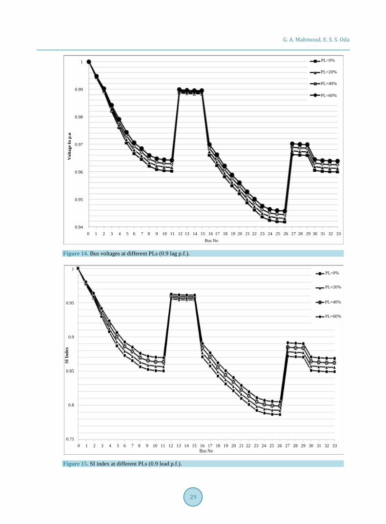
Study the voltage stability enhancement and PLR by installing WT at bus 5 of distribution feeder with differ-ent PL% listed in Table 11.

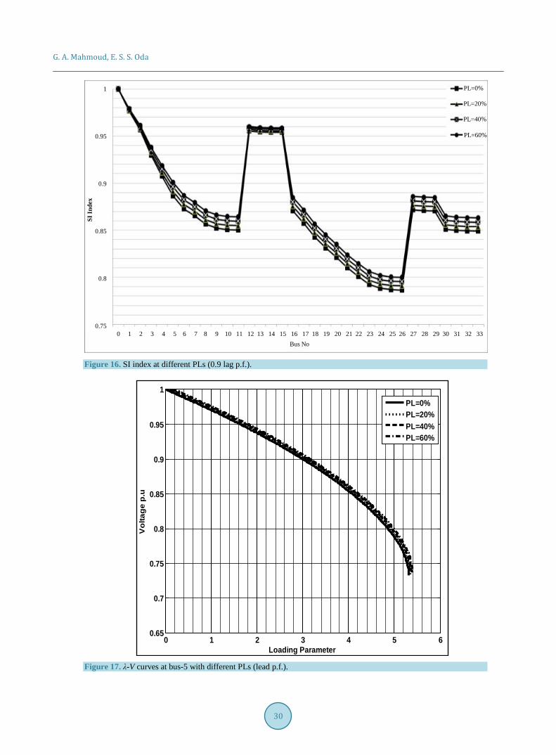
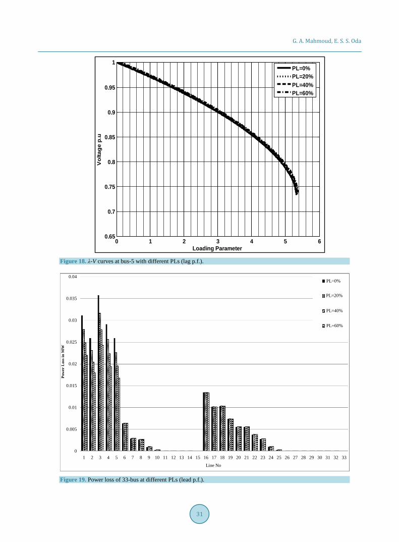
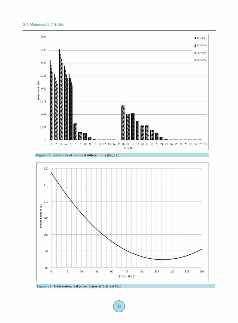
The Figures 13-20 show the impact of connection WT with different sizes and locations on voltage profile, SI index, λ-V curves, active losses, and reactive losses; while Figure 21 shows the relation between penetration level and power loss of the system.

Figure 9. Power losses of 9-bus feeder at different PLs (lead p.f.).

Table 1. Different PLs of WT.

Case 1 2 3 4

PL% 0% 20% 40% 60%

PWT (kW) 0.00 328 656 984

PL=0%

PL=40%

PL=60%

PL=20%

Pow

er L

oss i

n M

W

0.2

0.18

0.16

0.14

0.12

0.1

0.08

0.06

0.04

0.02

0

Line No1 2 3 4 5 6 7 8 9

G. A. Mahmoud, E. S. S. Oda

24

Figure 10. Power losses of 9-bus feeder at different PLs (lag p.f.).

Figure 11. Total system real power loss at different PLs.

PL=0%

PL=40%

PL=60%

PL=20%Po

wer

Los

s in

MW

Line No1 2 3 4 5 6 7 8 9

0.2

0.18

0.16

0.14

0.12

0.1

0.08

0.06

0.04

0.02

0

Syst

em P

owr

Los

s kw

PL% at Bus 90 20 40 60 80 100 120 140 160 180 200 220 240 260 280 300

800

700

600

500

400

300

200

G. A. Mahmoud, E. S. S. Oda

25

Table 2. Bus Voltages at different PLs (0.9 lead p.f.).

Bus No Bus Voltage in p.u

PL = 0% PL = 20% PL = 40% PL = 60%

0 1.00000 1.00000 1.00000 1.00000

1 0.99290 0.99323 0.99353 0.99382

2 0.98737 0.98801 0.98862 0.98920

3 0.96340 0.96527 0.96705 0.96874

4 0.94801 0.95077 0.95339 0.95589

5 0.91716 0.92240 0.92738 0.93213

6 0.90716 0.91350 0.91952 0.92527

7 0.88895 0.89750 0.90563 0.91340

8 0.85869 0.87227 0.88520 0.89756

9 0.83750 0.85648 0.87457 0.89188

Table 3. Bus voltages at different PLs (0.9 lag p.f.).

Bus No Bus Voltage in p.u

PL = 0% PL = 20% PL = 40% PL = 60%

0 1.00000 1.00000 1.00000 1.00000

1 0.99290 0.99295 0.99298 0.99300

2 0.98737 0.98734 0.98728 0.98719

3 0.96340 0.96376 0.96404 0.96425

4 0.94801 0.94881 0.94951 0.95010

5 0.91716 0.91917 0.92099 0.92263

6 0.90716 0.90969 0.91200 0.91409

7 0.88895 0.89280 0.89636 0.89964

8 0.85869 0.86550 0.87188 0.87786

9 0.83750 0.84742 0.85682 0.86573

Table 4. SI index at different PLs (0.9 lead p.f.).

Bus No SI Index

PL = 0% PL = 20% PL = 40% PL = 60%

0 1.00000 1.00000 1.00000 1.00000

1 0.97112 0.97244 0.97368 0.97487

2 0.94928 0.95185 0.95428 0.95658

3 0.85618 0.86336 0.87019 0.87671

4 0.80623 0.81584 0.82503 0.83385

5 0.70087 0.71804 0.73456 0.75052

6 0.67651 0.69575 0.71440 0.73254

7 0.62256 0.64729 0.67143 0.69507

8 0.53872 0.57522 0.61135 0.64720

9 0.48966 0.53668 0.58422 0.63232

G. A. Mahmoud, E. S. S. Oda

26

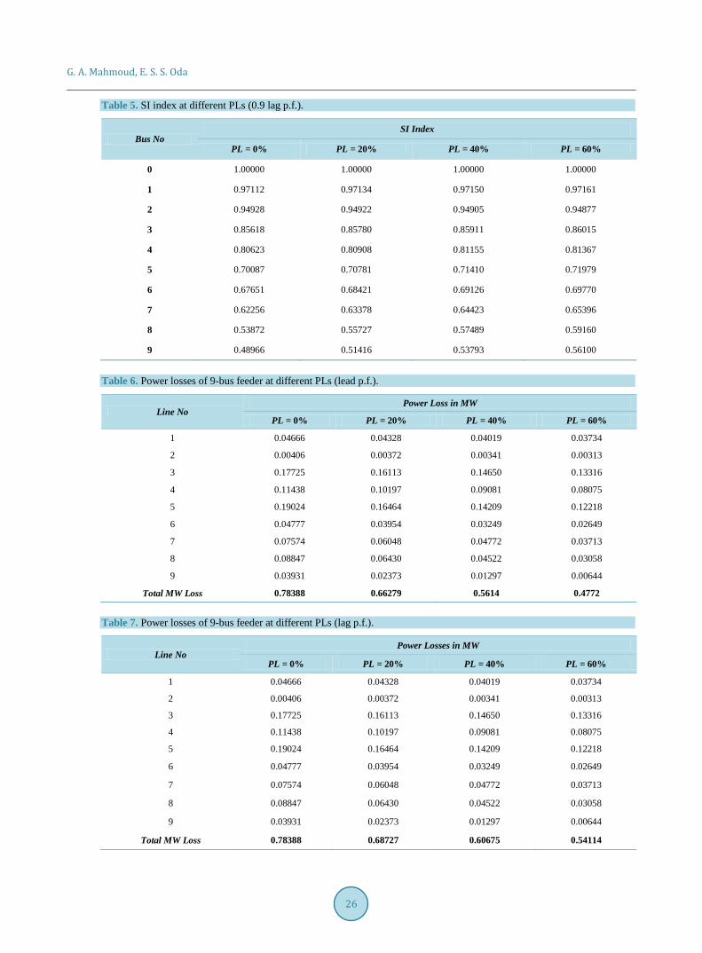
Table 5. SI index at different PLs (0.9 lag p.f.).

Bus No SI Index

PL = 0% PL = 20% PL = 40% PL = 60%

0 1.00000 1.00000 1.00000 1.00000

1 0.97112 0.97134 0.97150 0.97161

2 0.94928 0.94922 0.94905 0.94877

3 0.85618 0.85780 0.85911 0.86015

4 0.80623 0.80908 0.81155 0.81367

5 0.70087 0.70781 0.71410 0.71979

6 0.67651 0.68421 0.69126 0.69770

7 0.62256 0.63378 0.64423 0.65396

8 0.53872 0.55727 0.57489 0.59160

9 0.48966 0.51416 0.53793 0.56100

Table 6. Power losses of 9-bus feeder at different PLs (lead p.f.).

Line No Power Loss in MW

PL = 0% PL = 20% PL = 40% PL = 60%

1 0.04666 0.04328 0.04019 0.03734

2 0.00406 0.00372 0.00341 0.00313

3 0.17725 0.16113 0.14650 0.13316

4 0.11438 0.10197 0.09081 0.08075

5 0.19024 0.16464 0.14209 0.12218

6 0.04777 0.03954 0.03249 0.02649

7 0.07574 0.06048 0.04772 0.03713

8 0.08847 0.06430 0.04522 0.03058

9 0.03931 0.02373 0.01297 0.00644

Total MW Loss 0.78388 0.66279 0.5614 0.4772

Table 7. Power losses of 9-bus feeder at different PLs (lag p.f.).

Line No Power Losses in MW

PL = 0% PL = 20% PL = 40% PL = 60%

1 0.04666 0.04328 0.04019 0.03734

2 0.00406 0.00372 0.00341 0.00313

3 0.17725 0.16113 0.14650 0.13316

4 0.11438 0.10197 0.09081 0.08075

5 0.19024 0.16464 0.14209 0.12218

6 0.04777 0.03954 0.03249 0.02649

7 0.07574 0.06048 0.04772 0.03713

8 0.08847 0.06430 0.04522 0.03058

9 0.03931 0.02373 0.01297 0.00644

Total MW Loss 0.78388 0.68727 0.60675 0.54114

G. A. Mahmoud, E. S. S. Oda

27

Table 8. Voltage and voltage index of bus-9 in all cases.

Case 1 2 3 4

PL% 0% 20% 40% 60%

PWT (kW) 0.0000 328.00 656.00 984.00

0.9 Lead p.f

VBus-9 p.u 0.83750 0.85648 0.87457 0.89188

SIBus-9 0.48966 0.53668 0.58422 0.63232

λmax 2.0645 2.3026 2.5836 2.9045

PLoss (kW) 783.88 662.79 561.40 477.20

PLR% 0.00% 15.45% 28.38% 39.12%

0.9 Lag. p.f

VBus-9 p.u 0.83750 0.84742 0.85682 0.86573

SIBus-9 0.48966 0.51416 0.53793 0.56100

λmax 2.0645 2.2216 2.3874 2.5505

PLoss (kW) 783.88 687.27 606.75 541.14

PLR% 0.00% 12.32% 22.60% 30.96%

Table 9. Optimal size of WT at various buses.

Bus No Optimal Size of WT (MW) Line Losses (kW)

0 13.15 783.9

1 13.60 737.0

2 13.60 732.2

3 11.13 556.4

4 9.890 452.4

5 7.920 279.3

6 7.170 246.1

7 6.060 204.7

8 4.580 192.2

9 3.710 226.0

Table 10. Optimal location for installing WT on system.

WT Optimal Location Bus 8

WT optimal Size 4.57 MW

Active Power loss without WT 783.870 kW

Reactive Power loss without WT 1036.50 kVAr

Active Power loss with WT 192.16 kW

Reactive Power loss with WT 296.49 kVAr

Minimum Voltage without WT 0.83750 p.u (Bus 9)

Maximum Voltage without WT 1.00000 p.u (Bus 0)

Minimum Voltage with WT 0.95459 p.u (Bus 9)

Maximum Voltage with WT 1.00000 p.u (Bus 0)

G. A. Mahmoud, E. S. S. Oda

28

Table 11. Different PLs of WT.

Case 1 2 3 4

PL% 0% 20% 40% 60%

PWT (kW) 0.00 258.68 517.35 776.03

Figure 12. Single line diagram of feeder 33-bus laterals and sub-lateral.

Figure 13. Bus voltages at different PLs (0.9 lead p.f.).

G. A. Mahmoud, E. S. S. Oda

29

Figure 14. Bus voltages at different PLs (0.9 lag p.f.).

Figure 15. SI index at different PLs (0.9 lead p.f.).

PL=0%

PL=40%

PL=60%

PL=20%

Bus No0 1 2 3 4 5 6 7 8 9 10 11 12 13 14 15 16 17 18 19 20 21 22 23 24 25 26 27 28 29 30 31 32 33

Vol

tage

In p

.u1

0.99

0.98

0.97

0.96

0.95

0.94

PL=0%

PL=40%

PL=60%

PL=20%

Bus No0 1 2 3 4 5 6 7 8 9 10 11 12 13 14 15 16 17 18 19 20 21 22 23 24 25 26 27 28 29 30 31 32 33

SI In

dex

1

0.95

0.9

0.85

0.8

0.75

G. A. Mahmoud, E. S. S. Oda

30

Figure 16. SI index at different PLs (0.9 lag p.f.).

Figure 17. λ-V curves at bus-5 with different PLs (lead p.f.).

1

0.95

0.9

0.85

0.8

0.75

PL=0%

PL=40%

PL=60%

PL=20%

Bus No 0 1 2 3 4 5 6 7 8 9 10 11 12 13 14 15 16 17 18 19 20 21 22 23 24 25 26 27 28 29 30 31 32 33

SI In

dex

0 1 2 3 4 5 60.65

0.7

0.75

0.8

0.85

0.9

0.95

1

Loading Parameter

Vo

ltag

e p

.u

PL=0%PL=20%PL=40%PL=60%

G. A. Mahmoud, E. S. S. Oda

31

Figure 18. λ-V curves at bus-5 with different PLs (lag p.f.).

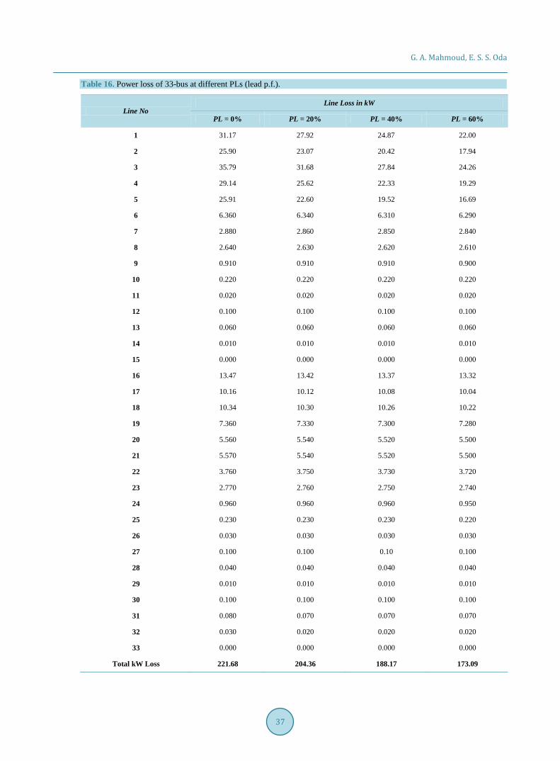
Figure 19. Power loss of 33-bus at different PLs (lead p.f.).

0 1 2 3 4 5 60.65

0.7

0.75

0.8

0.85

0.9

0.95

1

Loading Parameter

Vol

tage

p.u

PL=0%PL=20%PL=40%PL=60%

PL=0%

PL=40%

PL=60%

PL=20%

Line No

1 2 3 4 5 6 7 8 9 10 11 12 13 14 15 16 17 18 19 20 21 22 23 24 25 26 27 28 29 30 31 32 33

Pow

er L

oss i

n M

W

0.04

0.035

0.03

0.025

0.02

0.015

0.01

0.005

0

G. A. Mahmoud, E. S. S. Oda

32

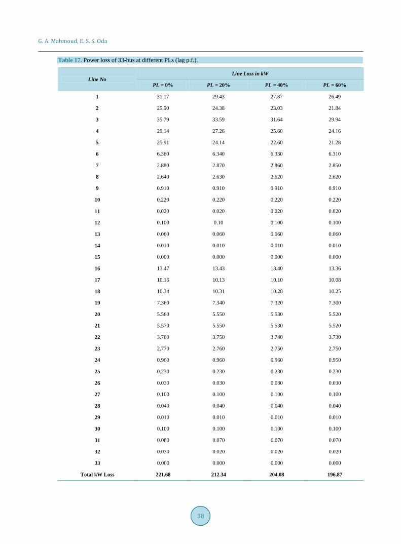
Figure 20. Power loss of 33-bus at different PLs (lag p.f.).

Figure 21. Total system real power losses at different PLs.

PL=0%

PL=40%

PL=60%

PL=20%

Line No 1 2 3 4 5 6 7 8 9 10 11 12 13 14 15 16 17 18 19 20 21 22 23 24 25 26 27 28 29 30 31 32 33

Pow

er L

oss i

n M

W0.04

0.035

0.03

0.025

0.02

0.015

0.01

0.005

0

PL% at Bus 5

0 15 30 45 60 75 90 105 120 135 150

Syst

em L

osse

s in

kw

120

115

110

105

100

95

90

G. A. Mahmoud, E. S. S. Oda

33

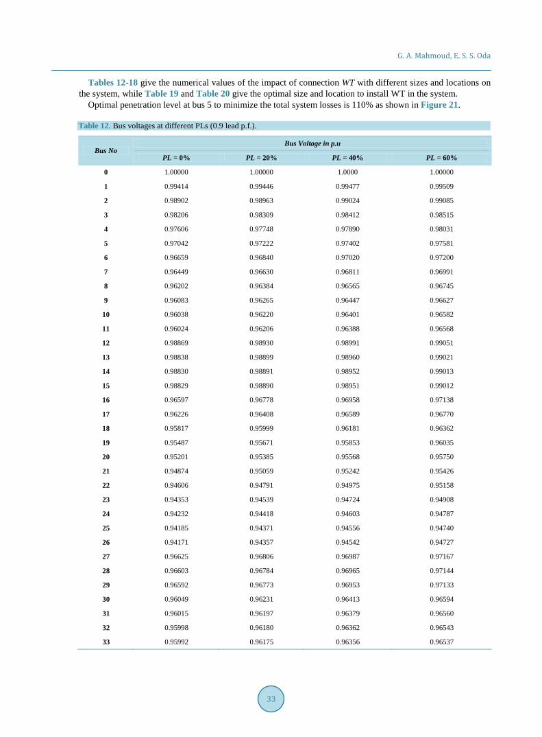
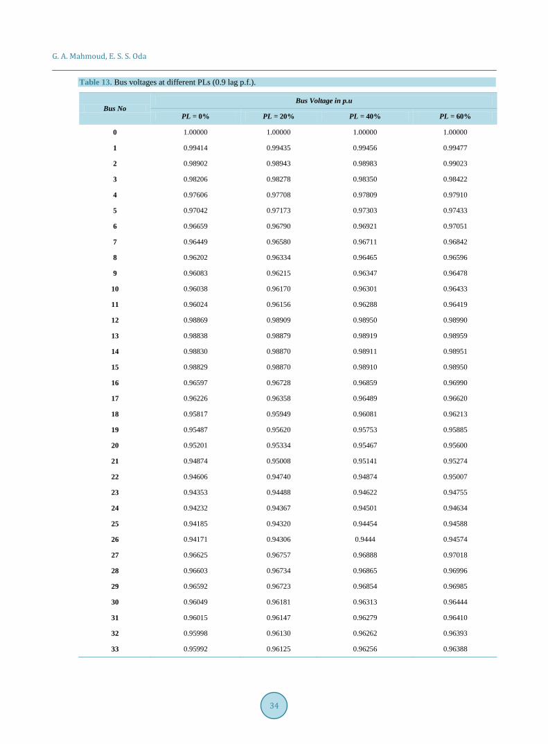
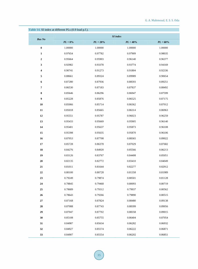
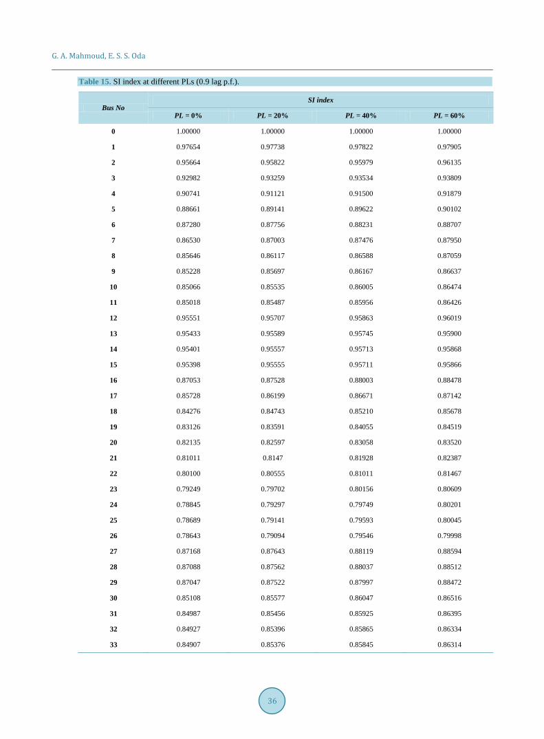
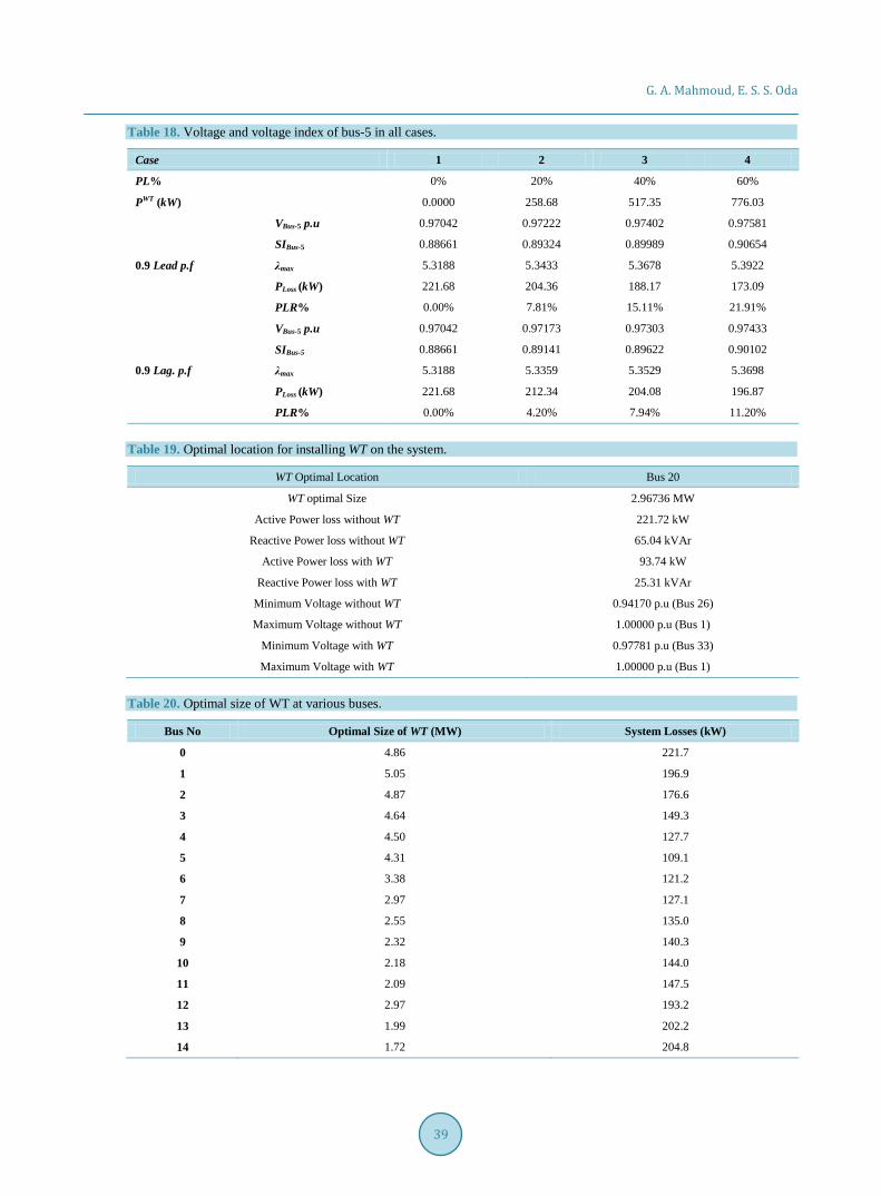
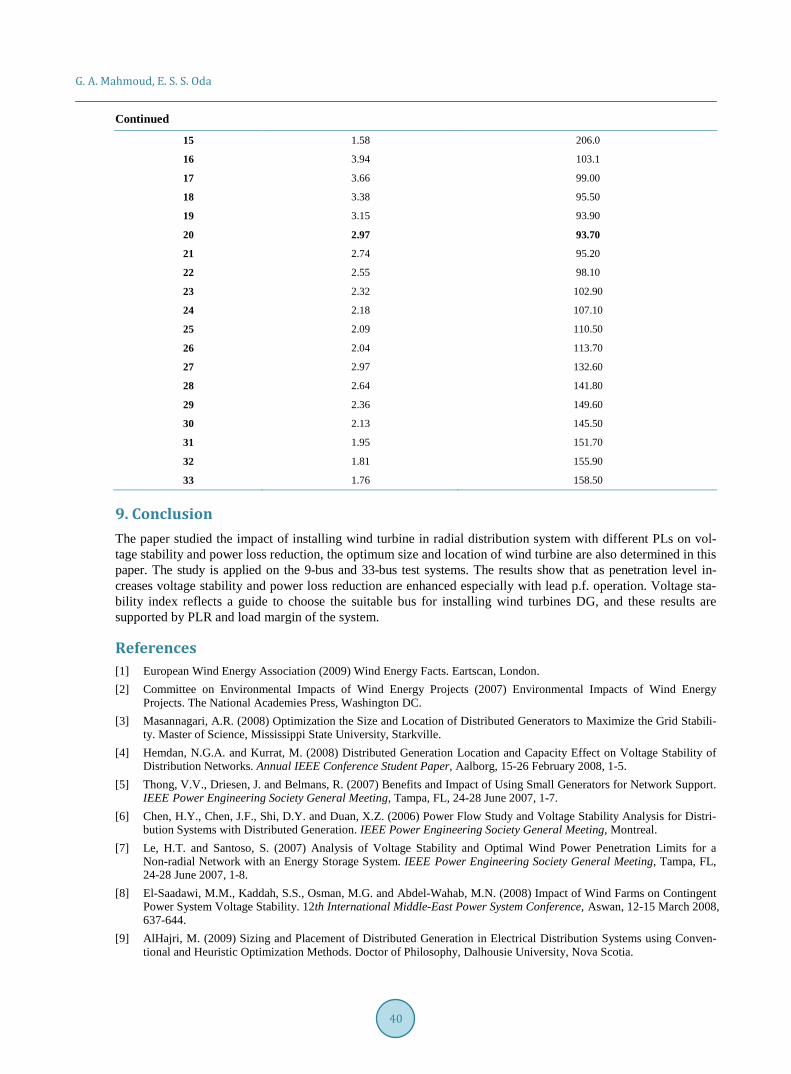
Tables 12-18 give the numerical values of the impact of connection WT with different sizes and locations on the system, while Table 19 and Table 20 give the optimal size and location to install WT in the system.

Optimal penetration level at bus 5 to minimize the total system losses is 110% as shown in Figure 21. Table 12. Bus voltages at different PLs (0.9 lead p.f.).

Bus No Bus Voltage in p.u

PL = 0% PL = 20% PL = 40% PL = 60%

0 1.00000 1.00000 1.0000 1.00000

1 0.99414 0.99446 0.99477 0.99509

2 0.98902 0.98963 0.99024 0.99085

3 0.98206 0.98309 0.98412 0.98515

4 0.97606 0.97748 0.97890 0.98031

5 0.97042 0.97222 0.97402 0.97581

6 0.96659 0.96840 0.97020 0.97200

7 0.96449 0.96630 0.96811 0.96991

8 0.96202 0.96384 0.96565 0.96745

9 0.96083 0.96265 0.96447 0.96627

10 0.96038 0.96220 0.96401 0.96582

11 0.96024 0.96206 0.96388 0.96568

12 0.98869 0.98930 0.98991 0.99051

13 0.98838 0.98899 0.98960 0.99021

14 0.98830 0.98891 0.98952 0.99013

15 0.98829 0.98890 0.98951 0.99012

16 0.96597 0.96778 0.96958 0.97138

17 0.96226 0.96408 0.96589 0.96770

18 0.95817 0.95999 0.96181 0.96362

19 0.95487 0.95671 0.95853 0.96035

20 0.95201 0.95385 0.95568 0.95750

21 0.94874 0.95059 0.95242 0.95426

22 0.94606 0.94791 0.94975 0.95158

23 0.94353 0.94539 0.94724 0.94908

24 0.94232 0.94418 0.94603 0.94787

25 0.94185 0.94371 0.94556 0.94740

26 0.94171 0.94357 0.94542 0.94727

27 0.96625 0.96806 0.96987 0.97167

28 0.96603 0.96784 0.96965 0.97144

29 0.96592 0.96773 0.96953 0.97133

30 0.96049 0.96231 0.96413 0.96594

31 0.96015 0.96197 0.96379 0.96560

32 0.95998 0.96180 0.96362 0.96543

33 0.95992 0.96175 0.96356 0.96537

G. A. Mahmoud, E. S. S. Oda

34

Table 13. Bus voltages at different PLs (0.9 lag p.f.).

Bus No Bus Voltage in p.u

PL = 0% PL = 20% PL = 40% PL = 60%

0 1.00000 1.00000 1.00000 1.00000

1 0.99414 0.99435 0.99456 0.99477

2 0.98902 0.98943 0.98983 0.99023

3 0.98206 0.98278 0.98350 0.98422

4 0.97606 0.97708 0.97809 0.97910

5 0.97042 0.97173 0.97303 0.97433

6 0.96659 0.96790 0.96921 0.97051

7 0.96449 0.96580 0.96711 0.96842

8 0.96202 0.96334 0.96465 0.96596

9 0.96083 0.96215 0.96347 0.96478

10 0.96038 0.96170 0.96301 0.96433

11 0.96024 0.96156 0.96288 0.96419

12 0.98869 0.98909 0.98950 0.98990

13 0.98838 0.98879 0.98919 0.98959

14 0.98830 0.98870 0.98911 0.98951

15 0.98829 0.98870 0.98910 0.98950

16 0.96597 0.96728 0.96859 0.96990

17 0.96226 0.96358 0.96489 0.96620

18 0.95817 0.95949 0.96081 0.96213

19 0.95487 0.95620 0.95753 0.95885

20 0.95201 0.95334 0.95467 0.95600

21 0.94874 0.95008 0.95141 0.95274

22 0.94606 0.94740 0.94874 0.95007

23 0.94353 0.94488 0.94622 0.94755

24 0.94232 0.94367 0.94501 0.94634

25 0.94185 0.94320 0.94454 0.94588

26 0.94171 0.94306 0.9444 0.94574

27 0.96625 0.96757 0.96888 0.97018

28 0.96603 0.96734 0.96865 0.96996

29 0.96592 0.96723 0.96854 0.96985

30 0.96049 0.96181 0.96313 0.96444

31 0.96015 0.96147 0.96279 0.96410

32 0.95998 0.96130 0.96262 0.96393

33 0.95992 0.96125 0.96256 0.96388

G. A. Mahmoud, E. S. S. Oda

35

Table 14. SI index at different PLs (0.9 lead p.f.).

Bus No SI index

PL = 0% PL = 20% PL = 40% PL = 60%

0 1.00000 1.00000 1.00000 1.00000

1 0.97654 0.97782 0.97909 0.98035

2 0.95664 0.95903 0.96140 0.96377

3 0.92982 0.93378 0.93774 0.94169

4 0.90741 0.91273 0.91804 0.92336

5 0.88661 0.89324 0.89989 0.90654

6 0.87280 0.87936 0.88593 0.89251

7 0.86530 0.87183 0.87837 0.88492

8 0.85646 0.86296 0.86947 0.87599

9 0.85228 0.85876 0.86525 0.87175

10 0.85066 0.85714 0.86362 0.87012

11 0.85018 0.85665 0.86314 0.86963

12 0.95551 0.95787 0.96023 0.96259

13 0.95433 0.95669 0.95905 0.96140

14 0.95401 0.95637 0.95873 0.96108

15 0.95398 0.95635 0.95870 0.96106

16 0.87053 0.87708 0.88365 0.89022

17 0.85728 0.86378 0.87029 0.87682

18 0.84276 0.84920 0.85566 0.86213

19 0.83126 0.83767 0.84408 0.85051

20 0.82135 0.82772 0.83410 0.84049

21 0.81011 0.81644 0.82277 0.82912

22 0.80100 0.80728 0.81358 0.81989

23 0.79249 0.79874 0.80501 0.81128

24 0.78845 0.79468 0.80093 0.80719

25 0.78689 0.79312 0.79937 0.80562

26 0.78643 0.79266 0.79890 0.80515

27 0.87168 0.87824 0.88480 0.89138

28 0.87088 0.87743 0.88399 0.89056

29 0.87047 0.87702 0.88358 0.89015

30 0.85108 0.85755 0.86404 0.87054

31 0.84987 0.85634 0.86282 0.86932

32 0.84927 0.85574 0.86222 0.86871

33 0.84907 0.85554 0.86202 0.86851

G. A. Mahmoud, E. S. S. Oda

36

Table 15. SI index at different PLs (0.9 lag p.f.).

Bus No SI index

PL = 0% PL = 20% PL = 40% PL = 60%

0 1.00000 1.00000 1.00000 1.00000

1 0.97654 0.97738 0.97822 0.97905

2 0.95664 0.95822 0.95979 0.96135

3 0.92982 0.93259 0.93534 0.93809

4 0.90741 0.91121 0.91500 0.91879

5 0.88661 0.89141 0.89622 0.90102

6 0.87280 0.87756 0.88231 0.88707

7 0.86530 0.87003 0.87476 0.87950

8 0.85646 0.86117 0.86588 0.87059

9 0.85228 0.85697 0.86167 0.86637

10 0.85066 0.85535 0.86005 0.86474

11 0.85018 0.85487 0.85956 0.86426

12 0.95551 0.95707 0.95863 0.96019

13 0.95433 0.95589 0.95745 0.95900

14 0.95401 0.95557 0.95713 0.95868

15 0.95398 0.95555 0.95711 0.95866

16 0.87053 0.87528 0.88003 0.88478

17 0.85728 0.86199 0.86671 0.87142

18 0.84276 0.84743 0.85210 0.85678

19 0.83126 0.83591 0.84055 0.84519

20 0.82135 0.82597 0.83058 0.83520

21 0.81011 0.8147 0.81928 0.82387

22 0.80100 0.80555 0.81011 0.81467

23 0.79249 0.79702 0.80156 0.80609

24 0.78845 0.79297 0.79749 0.80201

25 0.78689 0.79141 0.79593 0.80045

26 0.78643 0.79094 0.79546 0.79998

27 0.87168 0.87643 0.88119 0.88594

28 0.87088 0.87562 0.88037 0.88512

29 0.87047 0.87522 0.87997 0.88472

30 0.85108 0.85577 0.86047 0.86516

31 0.84987 0.85456 0.85925 0.86395

32 0.84927 0.85396 0.85865 0.86334

33 0.84907 0.85376 0.85845 0.86314

G. A. Mahmoud, E. S. S. Oda

37

Table 16. Power loss of 33-bus at different PLs (lead p.f.).

Line No Line Loss in kW

PL = 0% PL = 20% PL = 40% PL = 60%

1 31.17 27.92 24.87 22.00

2 25.90 23.07 20.42 17.94

3 35.79 31.68 27.84 24.26

4 29.14 25.62 22.33 19.29

5 25.91 22.60 19.52 16.69

6 6.360 6.340 6.310 6.290

7 2.880 2.860 2.850 2.840

8 2.640 2.630 2.620 2.610

9 0.910 0.910 0.910 0.900

10 0.220 0.220 0.220 0.220

11 0.020 0.020 0.020 0.020

12 0.100 0.100 0.100 0.100

13 0.060 0.060 0.060 0.060

14 0.010 0.010 0.010 0.010

15 0.000 0.000 0.000 0.000

16 13.47 13.42 13.37 13.32

17 10.16 10.12 10.08 10.04

18 10.34 10.30 10.26 10.22

19 7.360 7.330 7.300 7.280

20 5.560 5.540 5.520 5.500

21 5.570 5.540 5.520 5.500

22 3.760 3.750 3.730 3.720

23 2.770 2.760 2.750 2.740

24 0.960 0.960 0.960 0.950

25 0.230 0.230 0.230 0.220

26 0.030 0.030 0.030 0.030

27 0.100 0.100 0.10 0.100

28 0.040 0.040 0.040 0.040

29 0.010 0.010 0.010 0.010

30 0.100 0.100 0.100 0.100

31 0.080 0.070 0.070 0.070

32 0.030 0.020 0.020 0.020

33 0.000 0.000 0.000 0.000

Total kW Loss 221.68 204.36 188.17 173.09

G. A. Mahmoud, E. S. S. Oda

38

Table 17. Power loss of 33-bus at different PLs (lag p.f.).

Line No Line Loss in kW

PL = 0% PL = 20% PL = 40% PL = 60%

1 31.17 29.43 27.87 26.49

2 25.90 24.38 23.03 21.84

3 35.79 33.59 31.64 29.94

4 29.14 27.26 25.60 24.16

5 25.91 24.14 22.60 21.28

6 6.360 6.340 6.330 6.310

7 2.880 2.870 2.860 2.850

8 2.640 2.630 2.620 2.620

9 0.910 0.910 0.910 0.910

10 0.220 0.220 0.220 0.220

11 0.020 0.020 0.020 0.020

12 0.100 0.10 0.100 0.100

13 0.060 0.060 0.060 0.060

14 0.010 0.010 0.010 0.010

15 0.000 0.000 0.000 0.000

16 13.47 13.43 13.40 13.36

17 10.16 10.13 10.10 10.08

18 10.34 10.31 10.28 10.25

19 7.360 7.340 7.320 7.300

20 5.560 5.550 5.530 5.520

21 5.570 5.550 5.530 5.520

22 3.760 3.750 3.740 3.730

23 2.770 2.760 2.750 2.750

24 0.960 0.960 0.960 0.950

25 0.230 0.230 0.230 0.230

26 0.030 0.030 0.030 0.030

27 0.100 0.100 0.100 0.100

28 0.040 0.040 0.040 0.040

29 0.010 0.010 0.010 0.010

30 0.100 0.100 0.100 0.100

31 0.080 0.070 0.070 0.070

32 0.030 0.020 0.020 0.020

33 0.000 0.000 0.000 0.000

Total kW Loss 221.68 212.34 204.08 196.87

G. A. Mahmoud, E. S. S. Oda

39

Table 18. Voltage and voltage index of bus-5 in all cases.

Case 1 2 3 4

PL% 0% 20% 40% 60%

PWT (kW) 0.0000 258.68 517.35 776.03

0.9 Lead p.f

VBus-5 p.u 0.97042 0.97222 0.97402 0.97581

SIBus-5 0.88661 0.89324 0.89989 0.90654

λmax 5.3188 5.3433 5.3678 5.3922

PLoss (kW) 221.68 204.36 188.17 173.09

PLR% 0.00% 7.81% 15.11% 21.91%

0.9 Lag. p.f

VBus-5 p.u 0.97042 0.97173 0.97303 0.97433

SIBus-5 0.88661 0.89141 0.89622 0.90102

λmax 5.3188 5.3359 5.3529 5.3698

PLoss (kW) 221.68 212.34 204.08 196.87

PLR% 0.00% 4.20% 7.94% 11.20%

Table 19. Optimal location for installing WT on the system.

WT Optimal Location Bus 20

WT optimal Size 2.96736 MW

Active Power loss without WT 221.72 kW

Reactive Power loss without WT 65.04 kVAr

Active Power loss with WT 93.74 kW

Reactive Power loss with WT 25.31 kVAr

Minimum Voltage without WT 0.94170 p.u (Bus 26)

Maximum Voltage without WT 1.00000 p.u (Bus 1)

Minimum Voltage with WT 0.97781 p.u (Bus 33)

Maximum Voltage with WT 1.00000 p.u (Bus 1)

Table 20. Optimal size of WT at various buses.

Bus No Optimal Size of WT (MW) System Losses (kW)

0 4.86 221.7

1 5.05 196.9

2 4.87 176.6

3 4.64 149.3

4 4.50 127.7

5 4.31 109.1

6 3.38 121.2

7 2.97 127.1

8 2.55 135.0

9 2.32 140.3

10 2.18 144.0

11 2.09 147.5

12 2.97 193.2

13 1.99 202.2

14 1.72 204.8

G. A. Mahmoud, E. S. S. Oda

40

Continued 15 1.58 206.0

16 3.94 103.1

17 3.66 99.00

18 3.38 95.50

19 3.15 93.90

20 2.97 93.70

21 2.74 95.20

22 2.55 98.10

23 2.32 102.90

24 2.18 107.10

25 2.09 110.50

26 2.04 113.70

27 2.97 132.60

28 2.64 141.80

29 2.36 149.60

30 2.13 145.50

31 1.95 151.70

32 1.81 155.90

33 1.76 158.50

9. Conclusion The paper studied the impact of installing wind turbine in radial distribution system with different PLs on vol-tage stability and power loss reduction, the optimum size and location of wind turbine are also determined in this paper. The study is applied on the 9-bus and 33-bus test systems. The results show that as penetration level in-creases voltage stability and power loss reduction are enhanced especially with lead p.f. operation. Voltage sta-bility index reflects a guide to choose the suitable bus for installing wind turbines DG, and these results are supported by PLR and load margin of the system.

References [1] European Wind Energy Association (2009) Wind Energy Facts. Eartscan, London. [2] Committee on Environmental Impacts of Wind Energy Projects (2007) Environmental Impacts of Wind Energy

Projects. The National Academies Press, Washington DC. [3] Masannagari, A.R. (2008) Optimization the Size and Location of Distributed Generators to Maximize the Grid Stabili-

ty. Master of Science, Mississippi State University, Starkville. [4] Hemdan, N.G.A. and Kurrat, M. (2008) Distributed Generation Location and Capacity Effect on Voltage Stability of

Distribution Networks. Annual IEEE Conference Student Paper, Aalborg, 15-26 February 2008, 1-5. [5] Thong, V.V., Driesen, J. and Belmans, R. (2007) Benefits and Impact of Using Small Generators for Network Support.

IEEE Power Engineering Society General Meeting, Tampa, FL, 24-28 June 2007, 1-7. [6] Chen, H.Y., Chen, J.F., Shi, D.Y. and Duan, X.Z. (2006) Power Flow Study and Voltage Stability Analysis for Distri-

bution Systems with Distributed Generation. IEEE Power Engineering Society General Meeting, Montreal. [7] Le, H.T. and Santoso, S. (2007) Analysis of Voltage Stability and Optimal Wind Power Penetration Limits for a

Non-radial Network with an Energy Storage System. IEEE Power Engineering Society General Meeting, Tampa, FL, 24-28 June 2007, 1-8.

[8] El-Saadawi, M.M., Kaddah, S.S., Osman, M.G. and Abdel-Wahab, M.N. (2008) Impact of Wind Farms on Contingent Power System Voltage Stability. 12th International Middle-East Power System Conference, Aswan, 12-15 March 2008, 637-644.

[9] AlHajri, M. (2009) Sizing and Placement of Distributed Generation in Electrical Distribution Systems using Conven-tional and Heuristic Optimization Methods. Doctor of Philosophy, Dalhousie University, Nova Scotia.

G. A. Mahmoud, E. S. S. Oda

41

[10] Thukaram, D., Wijekoon Banda, H.M. and Jerome, J. (1999) A Robust Three Phase Power Flow Algorithm for Radial Distribution Systems. Electric Power Systems Research, 50, 227-236.

[11] Abu-Mouti, F.S. (2008) Radial Distribution Feeders Compensation Using Distributed Generation. Master of Applied Science, Dalhousie University, Nova Scotia.

[12] Khaniya, D. (2008) Development of Three Phase Continuation Power Flow for Voltage Stability Analysis of Distribu-tion System. Degree of Master of Science, Mississippi State University, Starkville.

[13] Verbič, G., Pantoš, M. and Gubina, F. (2006) On Voltage Collapse and Apparent-Power Losses. Electric Power Sys-tems Research, 76, 760-767. http://dx.doi.org/10.1016/j.epsr.2005.10.007

[14] IEEE/CIGRE Joint Task Force on Stability Terms and Definitions (2004) Definition and Classification of Power Sys-tem Stability. IEEE Transactions on Power Systems, 19, 1387-1401.

[15] Chakravorty, M. and Das, D. (2001) Voltage Stability Analysis of Radial Distribution Networks. Electrical Power and Energy Systems, 23, 129-135. http://dx.doi.org/10.1016/S0142-0615(00)00040-5

[16] Rao, S.S. (1996) Engineering Optimization: Theory and Practice. 3rd Edition, Wiley-Interscience, New York. [17] Goswami, S.K., Ghose, T. and Basu, S.K. (1999) An Approximate Method for Capacitor Placement in Distribution

System Using Heuristics and Greedy Search Technique. Electric Power Systems Research, 51, 143-151. http://dx.doi.org/10.1016/S0378-7796(98)00166-7

[18] Gözel, T., Eminoglu, U. and Hocaoglu, M.H. (2008) A Tool for Voltage Stability and Optimization (VS&OP) in Radi-al Distribution Systems Using Matlab Graphical User Interface (GUI). Simulation Modelling Practice and Theory, 16, 505-518. http://dx.doi.org/10.1016/j.simpat.2008.02.003

[19] Srinivasa Rao, R. (2010) Optimal Capacitor Allocation for loss reduction in Distribution System Using Fuzzy and Plant Growth Simulation Algorithm. International Journal of Computer, Electrical, Automation, Control and Informa-tion Engineering, 4, 1236-1242.

G. A. Mahmoud, E. S. S. Oda

42

Appendices Appendix A

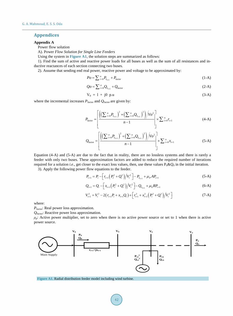
Power flow solution A). Power Flow Solution for Single Line Feeders Using the system in Figure A1, the solution steps are summarized as follows: 1). Find the sum of active and reactive power loads for all buses as well as the sum of all resistances and in-

ductive reactances of each section connecting two buses. 2). Assume that sending end real power, reactive power and voltage to be approximated by:

10 factori

ni LPo P P

+== +∑ (1-A)

10 factori

ni LQo Q Q

+== +∑ (2-A)

V0 = l + j0 p.u (3-A) where the incremental increases Pfactor and Qfactor are given by:

( ) ( )( )1 1

2 2 20 0

factor 0 11i i

n ni L i L

ni i

P Q VoP r

n+ += =

= +

+ = × −

∑ ∑∑ (4-A)

( ) ( )( )1 1

2 2 20 0

factor 0 11i i

n ni L i L

ni i

P Q VoQ x

n+ += =

= +

+ = × −

∑ ∑∑ (5-A)

Equation (4-A) and (5-A) are due to the fact that in reality, there are no lossless systems and there is rarely a feeder with only two buses. These approximation factors are added to reduce the required number of iterations required for a solution i.e., get closer to the exact loss values, then, use these values P0&Q0 in the initial iteration.

3). Apply the following power flow equations to the feeder.

( ) 1

2 2 21 1 1ii i i I i i L P iP P r P Q V P APµ

++ + + = − + − + (5-A)

( ) 1

2 2 21 1 0 1ii i i I i i L iQ Q x P Q V Q RPµ

++ + + = − + − + (6-A)

( ) ( )2 2 2 2 2 2 21 1 1 1 12i i i i i i i i i i iV V r P x Q r x P Q V+ + + + +

= − + + + + (7-A)

where: Pfactor: Real power loss approximation. Qfactor: Reactive power loss approximation. μp: Active power multiplier, set to zero when there is no active power source or set to 1 when there is active power source.

V0

P0Q0

ri+1+jxi+1

Vh Vk Vn

PnQn

PwtK

QwtK

PLkQLk

Main Supply

Figure A1. Radial distribution feeder model including wind turbine.

G. A. Mahmoud, E. S. S. Oda

43

μ0: Reactive power multiplier, set to zero when there is no reactive power source or set to ± 1 when there is a reactive power source. APi + 1:Active Power magnitude injected at bus i + 1 RPi + 1:Reactive Power magnitude injected at bus i + 1

4). If the absolute values of Pn & Qn of the last bus are zero or within an acceptable tolerance, the power flow solution is acceptable. Otherwise, go to the next step.

5). For the first bus in the main feeder set:

new oldO O nP P P= + (8-A)

new oldO O nQ Q Q= + (9-A)

Then, use these new initial values and repeat step 3. A). Power Flow Solution for Lateral and Sub-lateral Feeders: 1). Find the sum of real and reactive power loads on the sub-laterals (if available) and represent them as loads

on their laterals. Do the same for laterals and represent them as loads on the main feeder. 2). Apply the recursive power flow solution algorithm as in (single line feeders) for the main feeder. 3). Set the voltage of the far bus that represents a lateral to be equal to the (V0) of this lateral. Solve the lateral

individually as described in the case of the single line feeder. 4). For sub-laterals (if available), set the voltage of the far bus that represents a sub-lateral to be equal to the

(V0) of this sub-lateral. Solve the sub-lateral individually as described in the case of the single line feeder. 5). Get the total real and reactive powers injected into the sub-lateral and represent them again as a single load

on its lateral. 6). Apply the power flow solution to the lateral individually again. If there is another sub-lateral go back to

step 4 and solve the second far bus on the lateral that represents the sub-lateral. Otherwise, go to next step. 7). Find the total real and reactive powers injected into the lateral (use data from last power flow run) and

represent them again as a load on the main feeder. 8). Apply the power flow recursion to the main feeder. If there are more laterals, go back to step 3 and solve

for the second far bus that represents the lateral on the main feeder. If not, go to the next step. 9). With the bus voltages found using the previous step, solve the laterals and sub-laterals (if available) indi-

vidually. Then the power flow solution is reached.

G. A. Mahmoud, E. S. S. Oda

44

Appendix B

Figure B-1. Flowchart of the grid search algorithm.

G. A. Mahmoud, E. S. S. Oda

45

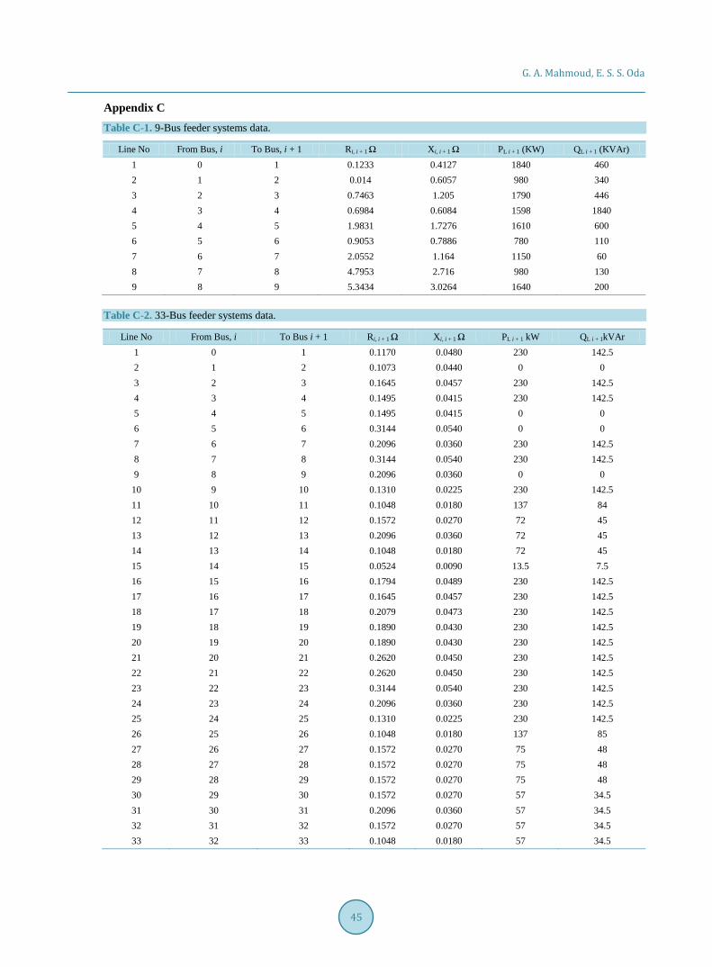
Appendix C Table C-1. 9-Bus feeder systems data.

Line No From Bus, i To Bus, i + 1 Ri, i + 1 Ω Xi, i + 1 Ω PL i + 1 (KW) QL i + 1 (KVAr) 1 0 1 0.1233 0.4127 1840 460 2 1 2 0.014 0.6057 980 340 3 2 3 0.7463 1.205 1790 446 4 3 4 0.6984 0.6084 1598 1840 5 4 5 1.9831 1.7276 1610 600 6 5 6 0.9053 0.7886 780 110 7 6 7 2.0552 1.164 1150 60 8 7 8 4.7953 2.716 980 130 9 8 9 5.3434 3.0264 1640 200

Table C-2. 33-Bus feeder systems data.

Line No From Bus, i To Bus i + 1 Ri, i + 1 Ω Xi, i + 1 Ω PL i + 1 kW QL i + 1kVAr 1 0 1 0.1170 0.0480 230 142.5 2 1 2 0.1073 0.0440 0 0 3 2 3 0.1645 0.0457 230 142.5 4 3 4 0.1495 0.0415 230 142.5 5 4 5 0.1495 0.0415 0 0 6 5 6 0.3144 0.0540 0 0 7 6 7 0.2096 0.0360 230 142.5 8 7 8 0.3144 0.0540 230 142.5 9 8 9 0.2096 0.0360 0 0

10 9 10 0.1310 0.0225 230 142.5 11 10 11 0.1048 0.0180 137 84 12 11 12 0.1572 0.0270 72 45 13 12 13 0.2096 0.0360 72 45 14 13 14 0.1048 0.0180 72 45 15 14 15 0.0524 0.0090 13.5 7.5 16 15 16 0.1794 0.0489 230 142.5 17 16 17 0.1645 0.0457 230 142.5 18 17 18 0.2079 0.0473 230 142.5 19 18 19 0.1890 0.0430 230 142.5 20 19 20 0.1890 0.0430 230 142.5 21 20 21 0.2620 0.0450 230 142.5 22 21 22 0.2620 0.0450 230 142.5 23 22 23 0.3144 0.0540 230 142.5 24 23 24 0.2096 0.0360 230 142.5 25 24 25 0.1310 0.0225 230 142.5 26 25 26 0.1048 0.0180 137 85 27 26 27 0.1572 0.0270 75 48 28 27 28 0.1572 0.0270 75 48 29 28 29 0.1572 0.0270 75 48 30 29 30 0.1572 0.0270 57 34.5 31 30 31 0.2096 0.0360 57 34.5 32 31 32 0.1572 0.0270 57 34.5 33 32 33 0.1048 0.0180 57 34.5