Investigating Fluorescence Lifetime Spectroscopy & Imaging

David Birch

Department of PhysicsUniversity of StrathclydeGlasgow G4 0NGScotland

Content

• Fluorescence lifetime and its measurement

• Use in spectroscopy and microscopy

• Applications –

1. Glucose sensing

2. ββββ-amyloid fibrils

3. Nanoparticle metrology

» Focus on aromatic fluorophores

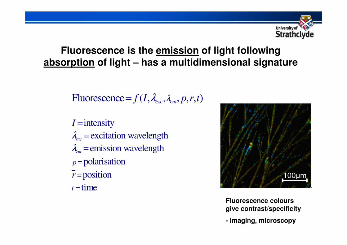
Fluorescence is the emission of light following absorption of light – has a multidimensional signature

,

intensity

=excitation wavelength

=emission wavelength

polarisation

position

time

Fluorescence ( , , , , )

exc

em

exc em

p

t

I

r

f I p r tλ

λ

λ

λ

=

=

=

=

=

Fluorescence colours

give contrast/specificity

- imaging, microscopy

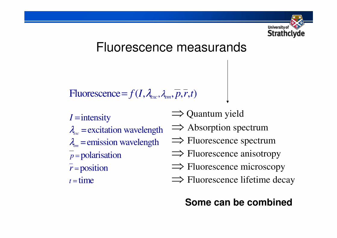
Fluorescence measurands

,

intensity

=excitation wavelength

=emission wavelength

polarisation

position

time

Fluorescence ( , , , , )

exc

em

exc em

p

t

I

r

f I p r tλ

λ

λ

λ

=

=

=

=

=

⇒ Quantum yield

⇒ Absorption spectrum

⇒ Fluorescence spectrum

⇒ Fluorescence anisotropy

⇒ Fluorescence microscopy

⇒ Fluorescence lifetime decay

Some can be combined

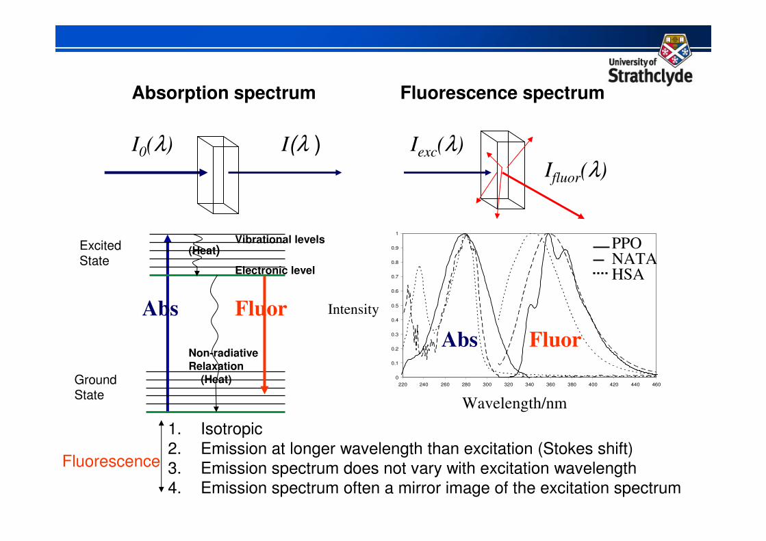
1. Isotropic

2. Emission at longer wavelength than excitation (Stokes shift)

3. Emission spectrum does not vary with excitation wavelength

4. Emission spectrum often a mirror image of the excitation spectrum

0

0.1

0.2

0.3

0.4

0.5

0.6

0.7

0.8

0.9

1

220 240 260 280 300 320 340 360 380 400 420 440 460

Fluorescence spectrum

Iexc(λ)

Ifluor(λ)

I0(λ)

Absorption spectrum

I(λ )

Excited State

GroundState

Abs Fluor

Non-radiative

Relaxation

(Heat)

Wavelength/nm

Intensity

PPONATAHSA

FluorAbs

Fluorescence

Vibrational levels

Electronic level

(Heat)

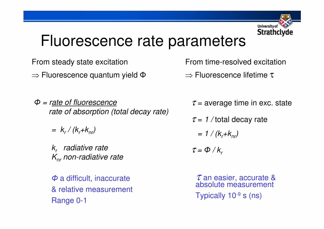
Fluorescence rate parameters

From steady state excitation From time-resolved excitation

⇒ Fluorescence quantum yield Φ ⇒ Fluorescence lifetime τ

= kr / (kr+knr)

Φ = rate of fluorescencerate of absorption (total decay rate)

τ = average time in exc. state

τ = 1 / total decay rate

= 1 / (kr+knr)

τ = Φ / kr

Φ a difficult, inaccurate

& relative measurement

Range 0-1

τ an easier, accurate & absolute measurement

Typically 10-9 s (ns)

kr radiative rate Knr non-radiative rate

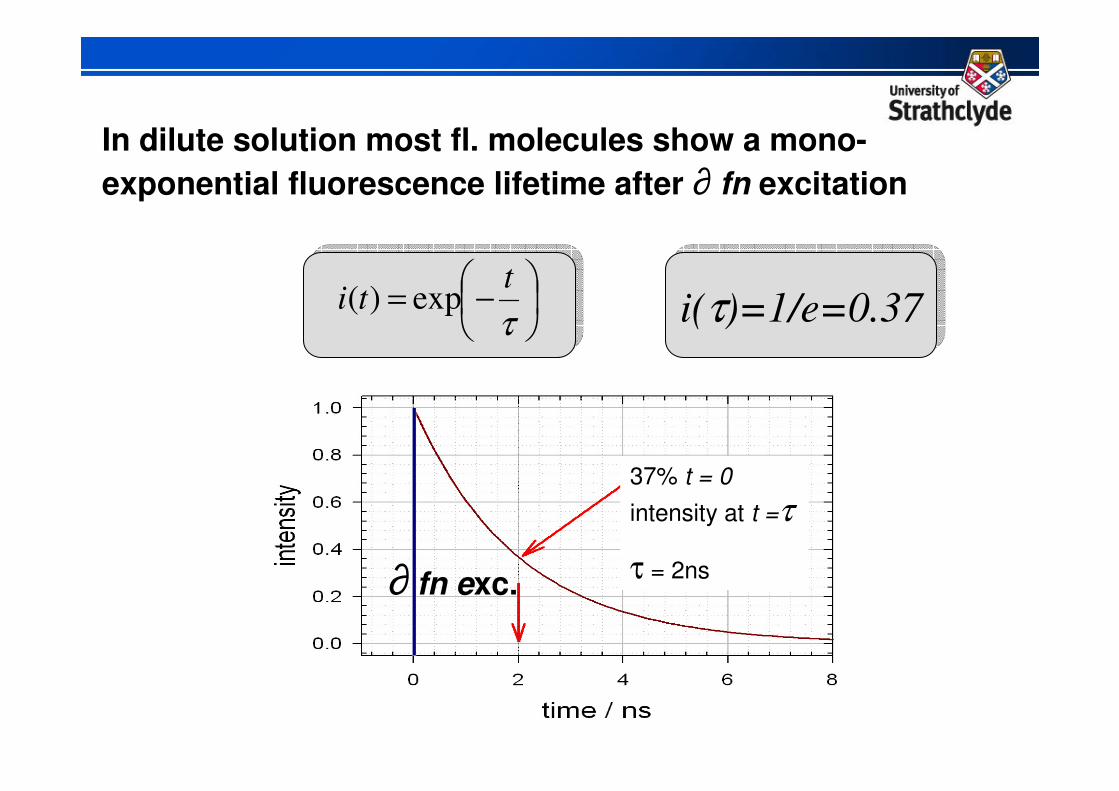
In dilute solution most fl. molecules show a mono-

exponential fluorescence lifetime after ∂ fn excitation

−=

τ

tti exp)(

τ τ τ τ = 2 ns

i(τ)=1/e=0.37i(τ)=1/e=0.37

∂ fn exc.

37% t = 0

intensity at t =τ

τ = 2ns

Real photon counting data has known noise statistics - Poisson

1 std. dev. at each datum

= √Ni

Where Ni is the

number of counts

at channel/time i

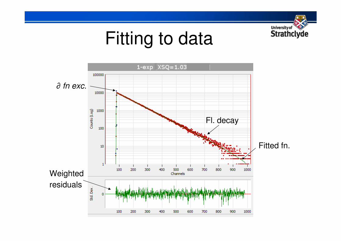
Fitting to data

Weighted

residuals

Fitted fn.

∂ fn exc.

Fl. decay

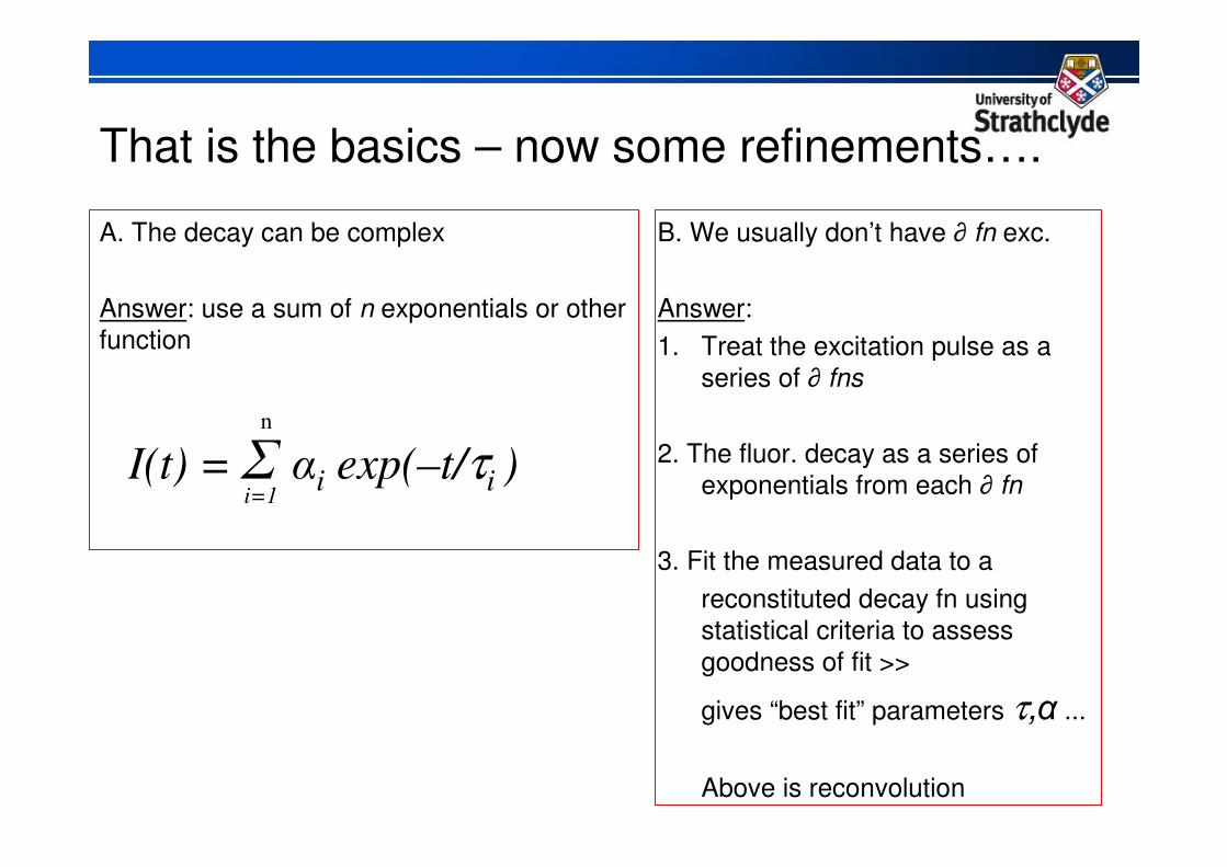
That is the basics – now some refinements….

A. The decay can be complex

Answer: use a sum of n exponentials or other

function

B. We usually don’t have ∂ fn exc.

Answer:

1. Treat the excitation pulse as a

series of ∂ fns

2. The fluor. decay as a series of

exponentials from each ∂ fn

3. Fit the measured data to a

reconstituted decay fn using

statistical criteria to assess

goodness of fit >>

gives “best fit” parameters τ,α ...

Above is reconvolution

I(t) = Σ αi exp(–t/τi )i=1

n

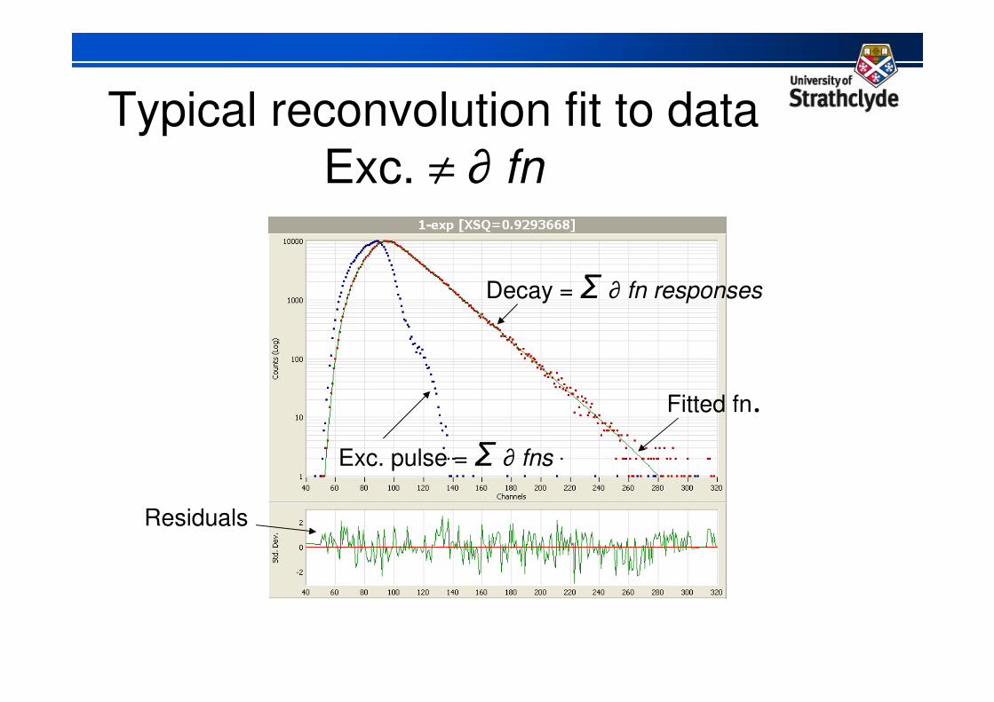
Typical reconvolution fit to data

Exc. ≠ ∂ fn

Decay = Σ ∂ fn responses

Exc. pulse = Σ ∂ fns

Fitted fn.

Residuals

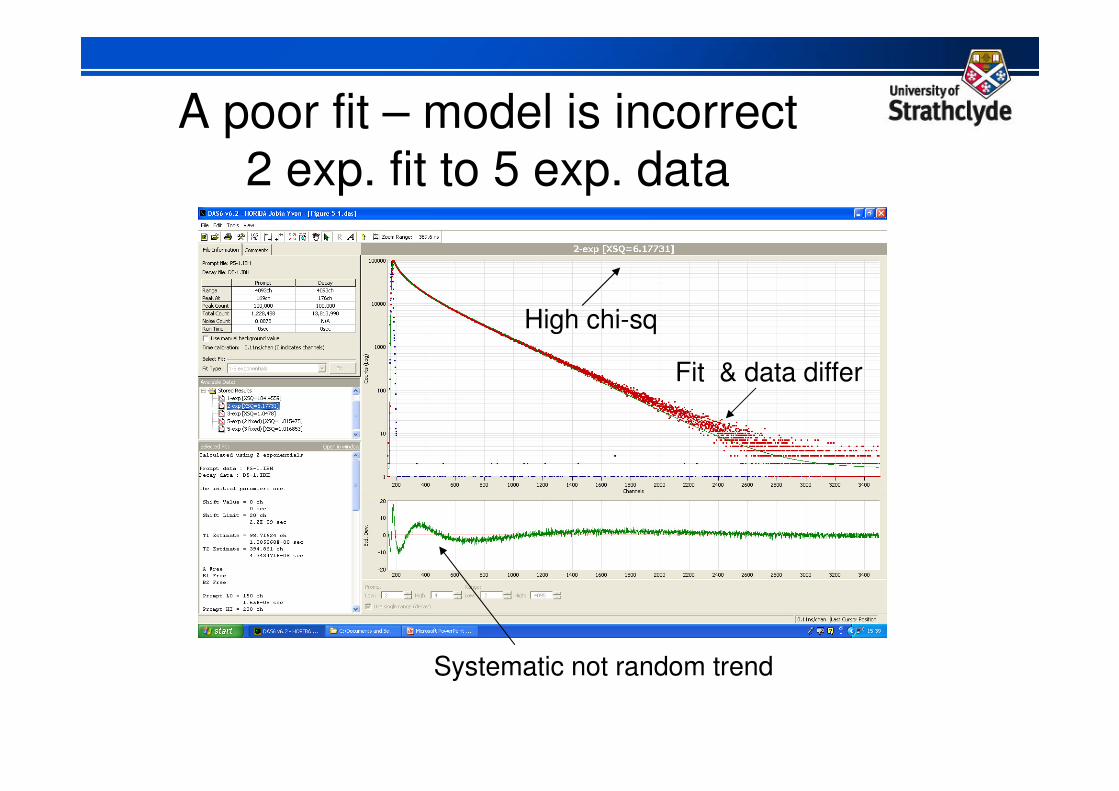
A poor fit – model is incorrect

2 exp. fit to 5 exp. data

High chi-sq

Systematic not random trend

Fit & data differ

0

2000

4000

6000

8000

10000

12000

1 2 3 4 5 6 7 8 9 10

11

12

13

14

15

16

17

18

19

20

21

22

23

24

25

26

27

28

29

30

31

32

33

34

35

36

TIME, CHANNELS

PH

OT

ON

CO

UN

TS

S

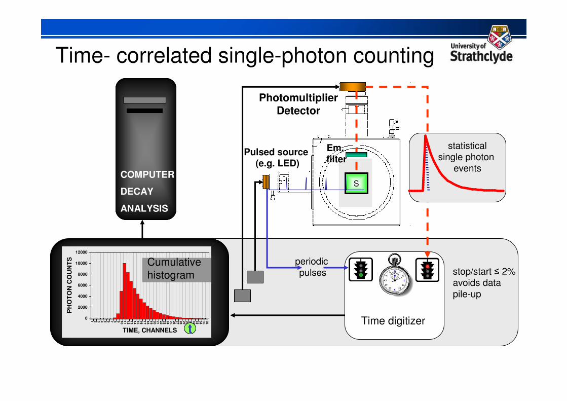
Pulsed source(e.g. LED)

stop/start ≤ 2% avoids data pile-up

statisticalsingle photon

events

periodic pulses

Time digitizer

Em. filter

t

Time- correlated single-photon counting

Cumulative

histogram

COMPUTER

DECAY

ANALYSIS

Photomultiplier Detector

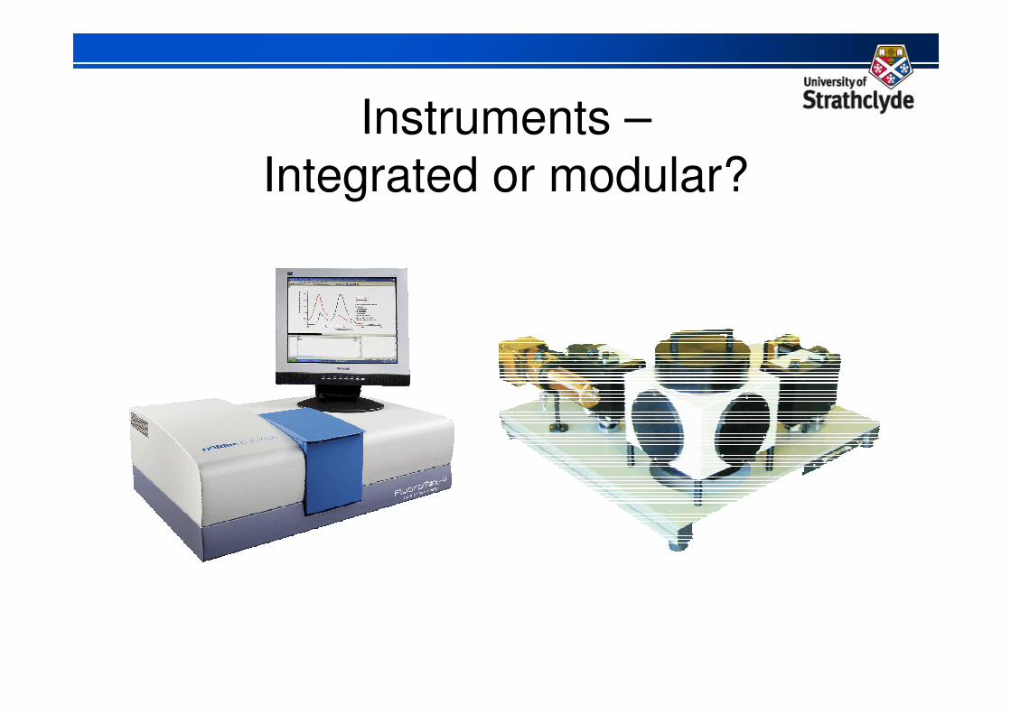
Instruments –

Integrated or modular?

Advantages of Fluorescence Lifetimes

Easy, accurate & absolute measurement

Digital not analogue technique - single-photon sensitivity & known statistics

Gives kinetic rates & dynamic information

Concentration independent – overcomes photo-bleaching

Extra specificity – can discriminate against background fluorescence,

scattered excitation etc

Includes fluorescence virtues - Stokes red shift, single-molecule

detection, compatible with optoelectronics (200 – 1000 nm)

Probe of nano-environment – pH, polarity, quenching, energy transfer, analyte specific interactions, etc

1st application – in-vivo glucose sensing

The Problem of Diabetes Mellitus -

• A condition characterized by a chronically raised blood glucose concentration due to a relative or absolute lack of insulin (Type I)

• 250 million people have diabetes worldwide (~ 7.5 x HIV/AIDS)

• 3.8 million people die from diabetes every year

• 10% of healthcare spending in many countries

• Maintaining normal glucose levels minimises complications –blindness, kidney disease, arteriosclerosis, poor circulation

• Grand challenge - No non-invasive and continuous glucose sensor exists

• Glucose metabolic range ~ 5 – 30 mM

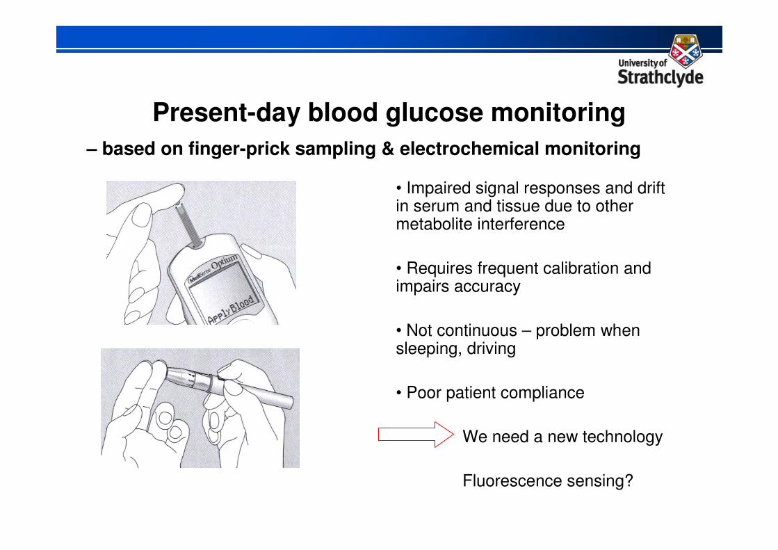
Present-day blood glucose monitoring

• Impaired signal responses and drift in serum and tissue due to other metabolite interference

• Requires frequent calibration and impairs accuracy

• Not continuous – problem when sleeping, driving

• Poor patient compliance

We need a new technology

Fluorescence sensing?

– based on finger-prick sampling & electrochemical monitoring

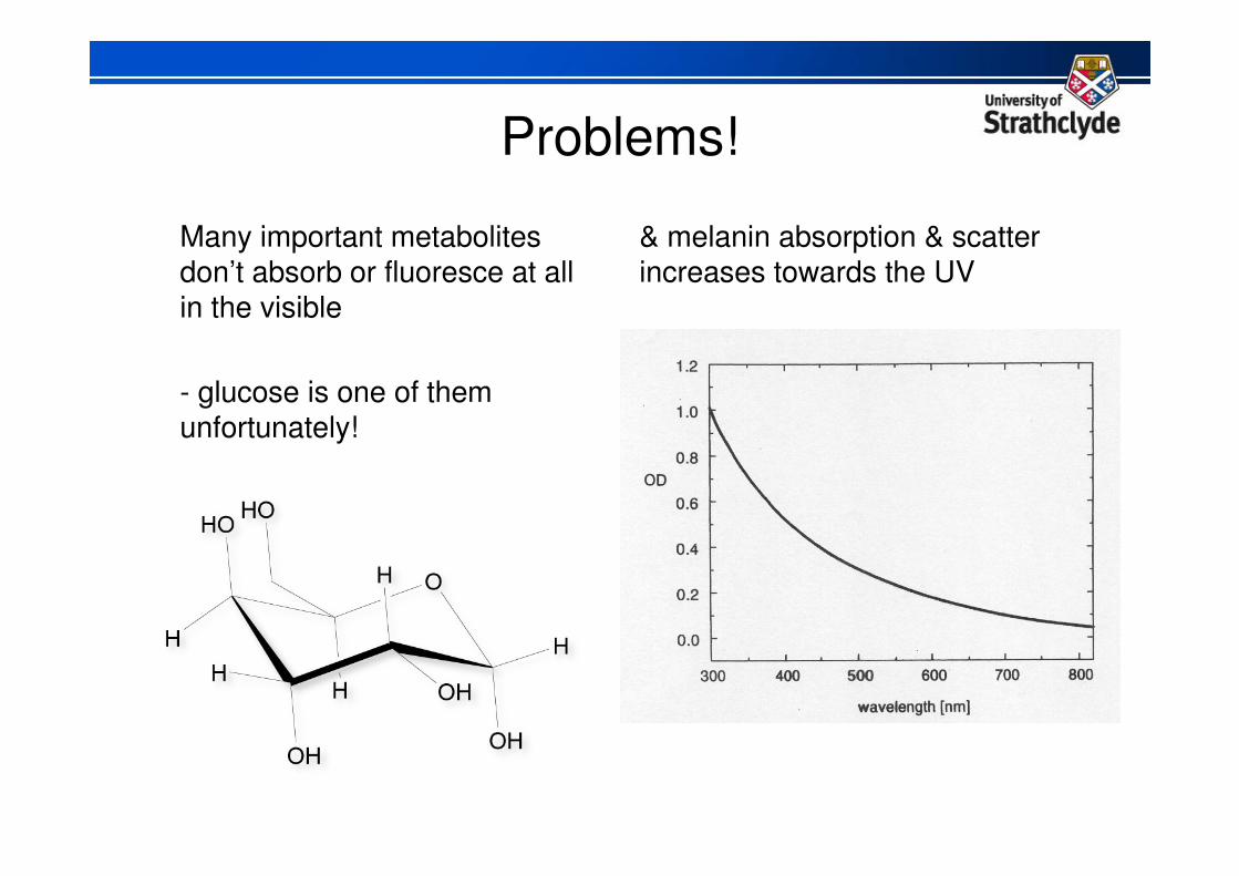
Problems!

Many important metabolites don’t absorb or fluoresce at all in the visible

- glucose is one of them unfortunately!

& melanin absorption & scatter increases towards the UV

Excited State

GroundState

Abs Fluor

Non-radiative

Relaxation

(Heat)

Vibrational levels

Electronic level

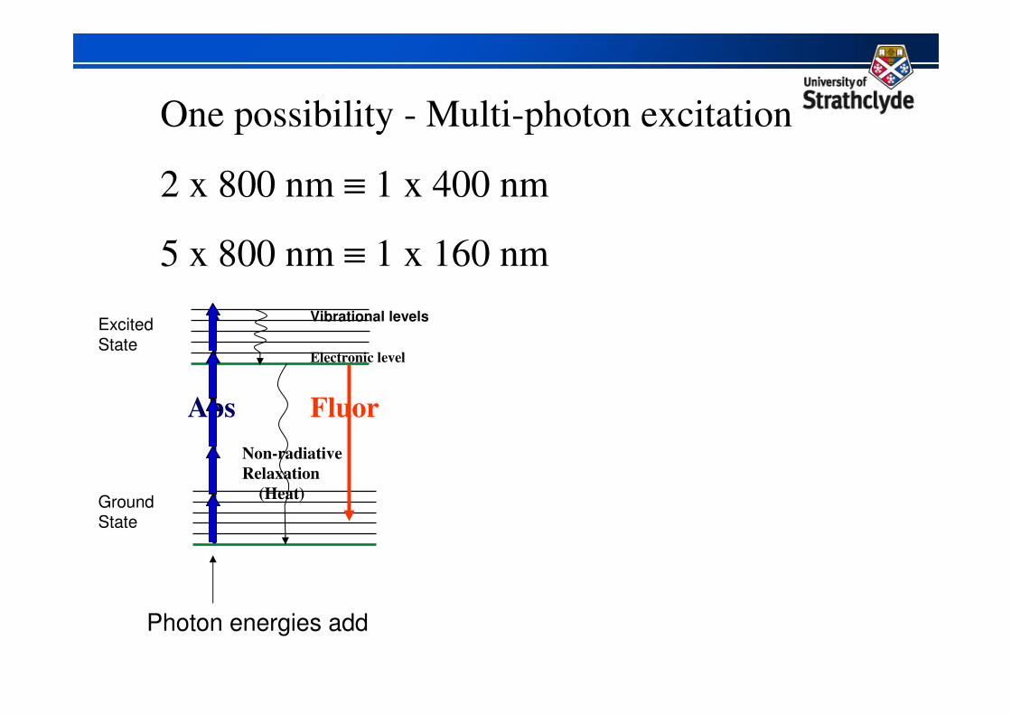
One possibility - Multi-photon excitation

2 x 800 nm ≡ 1 x 400 nm

5 x 800 nm ≡ 1 x 160 nm

Photon energies add

Excited State

GroundState

Abs Fluor

Non-radiative

Relaxation

(Heat)

Vibrational levels

Electronic level

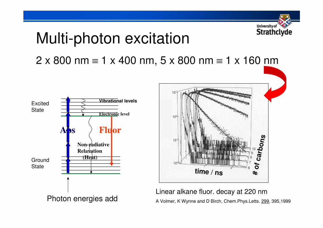
Multi-photon excitation

2 x 800 nm ≡ 1 x 400 nm, 5 x 800 nm ≡ 1 x 160 nm

Linear alkane fluor. decay at 220 nm

A Volmer, K Wynne and D Birch, Chem.Phys.Letts. 299, 395,1999

# o

f carb

on

s

time / ns

Photon energies add

But multi-photon excitation needs femtosecond laser exc. -Expensive, complex and impractical for a miniaturized sensor

Also – UV fluorescence will be filtered out by melanin

Answer –

use an extrinsic fluorescent probe & an indirect assay

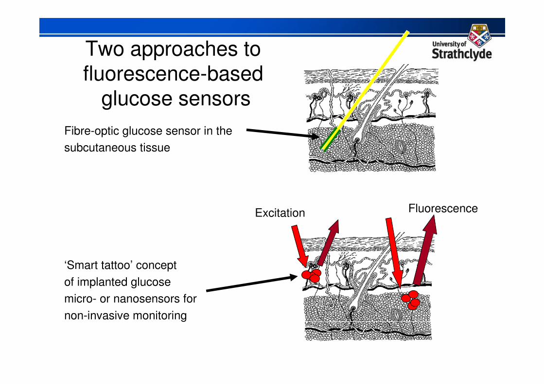
Two approaches to fluorescence-based

glucose sensors

Fibre-optic glucose sensor in the

subcutaneous tissue

‘Smart tattoo’ concept

of implanted glucose

micro- or nanosensors for

non-invasive monitoring

Excitation Fluorescence

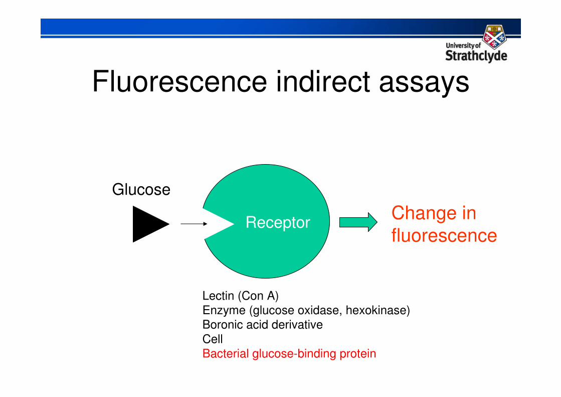
Fluorescence indirect assays

Receptor

Glucose

Change in

fluorescence

Lectin (Con A)

Enzyme (glucose oxidase, hexokinase)

Boronic acid derivative

Cell

Bacterial glucose-binding protein

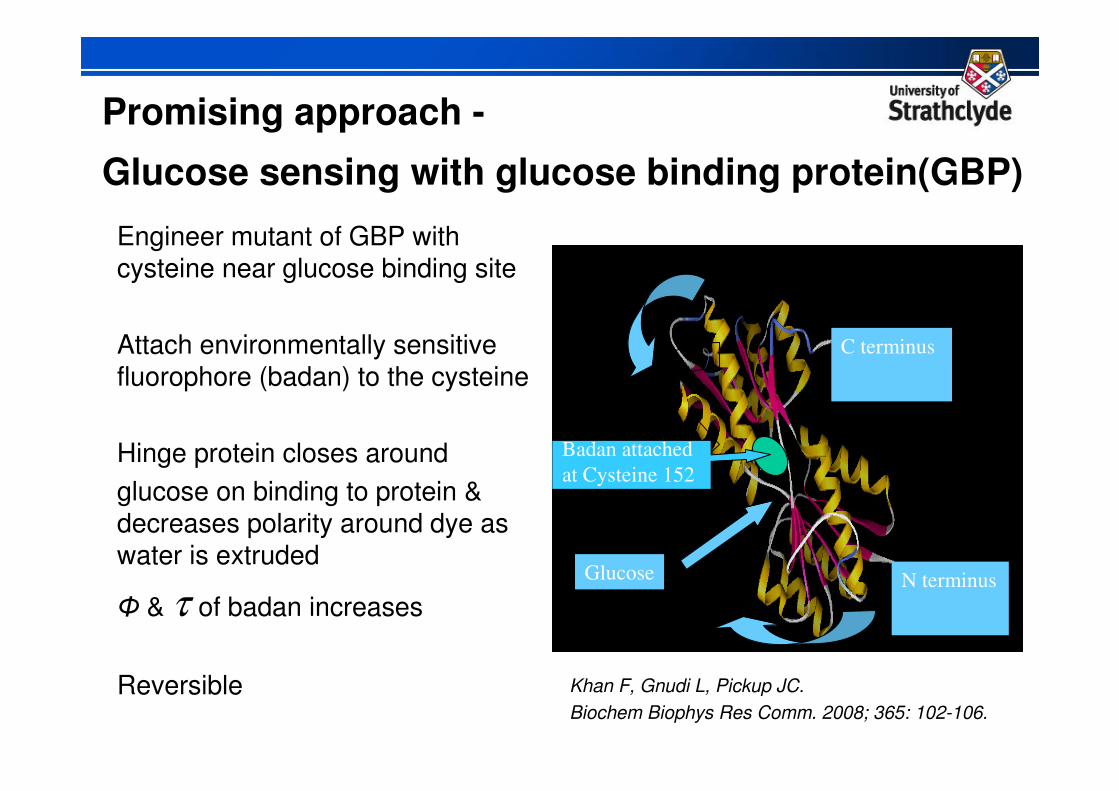
Promising approach -

Glucose sensing with glucose binding protein(GBP)

Engineer mutant of GBP with cysteine near glucose binding site

Attach environmentally sensitive fluorophore (badan) to the cysteine

Hinge protein closes around

glucose on binding to protein & decreases polarity around dye as water is extruded

Φ & τ of badan increases

Reversible

C terminus

N terminusGlucose

Badan attached

at Cysteine 152

Khan F, Gnudi L, Pickup JC.

Biochem Biophys Res Comm. 2008; 365: 102-106.

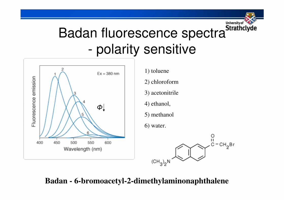
Badan fluorescence spectra

- polarity sensitive

1) toluene

2) chloroform

3) acetonitrile

4) ethanol,

5) methanol

6) water.

Badan - 6-bromoacetyl-2-dimethylaminonaphthalene

Φ

Fluorescence lifetime of badan

Fluorescence

decay in water

Fluorescence decay in organic solvent

In Water

Glucose increases encapsulated GBP-Badan fluorescence by ~ 300%

GBP-Badan capsules without glucose

GBP-Badan capsules with

100 µM glucose

λex = 400 nm

λem = 550 nm

GBP-Badan capsules without glucose

GBP-Badan capsules with

100 µM glucose

λex = 400 nm

λem = 550 nm

CaCO3CaCO3 CaCO3

GBP-B

GBP-Badan poly-lysine and poly-

glutamic acid layers

Template

dissolution

with EDTA

5µm

Encapsulation -

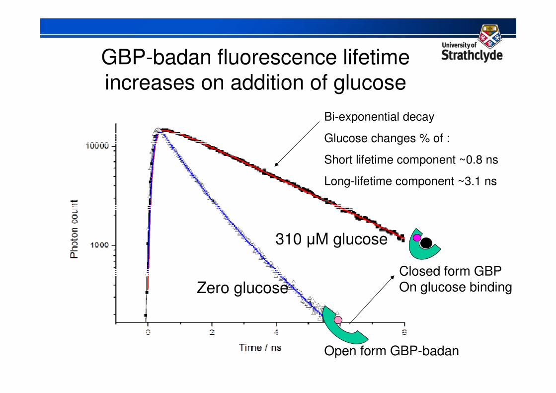
GBP-badan fluorescence lifetime increases on addition of glucose

Bi-exponential decay

Glucose changes % of :

Short lifetime component ~0.8 ns

Long-lifetime component ~3.1 ns

310 µM glucose

Zero glucose

Open form GBP-badan

Closed form GBPOn glucose binding

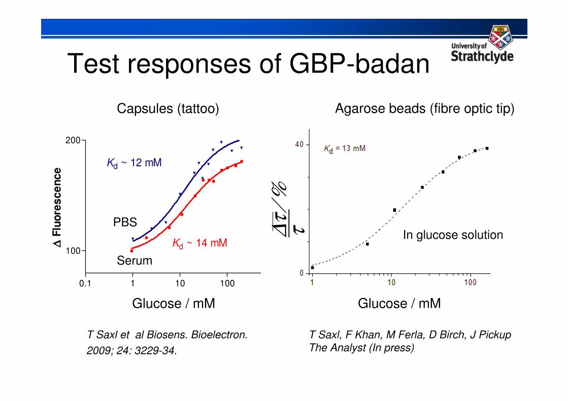
Test responses of GBP-badan

0.1 1 10 100 1000

100

200

Kd ~ 14 mM

PBS

Kd ~ 12 mM Serum

[glucose] mM

∆∆ ∆∆ F

luo

res

ce

nc

e

PBS

Serum

∆τ

⁄%τ

Glucose / mMGlucose / mM

Capsules (tattoo) Agarose beads (fibre optic tip)

In glucose solution

T Saxl, F Khan, M Ferla, D Birch, J Pickup

The Analyst (In press)

T Saxl et al Biosens. Bioelectron.

2009; 24: 3229-34.

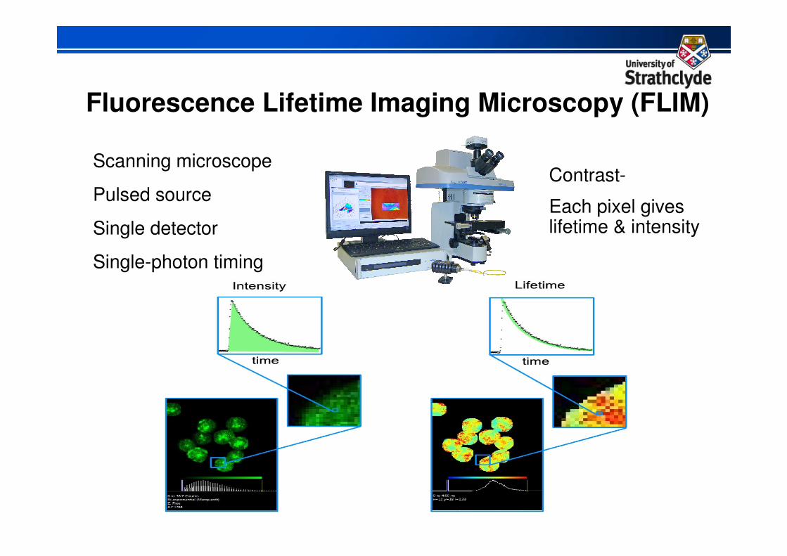
Fluorescence Lifetime Imaging Microscopy (FLIM)

Contrast-

Each pixel gives lifetime & intensity

Scanning microscope

Pulsed source

Single detector

Single-photon timing

Optimising Agarose beads with FLIM of bound GBP-Badan in PBS. excitation 400 nm, fluorescence 550 nm

fl. intensity image

Fluorescence lifetime images of beads(1 exp fit)

Zero glucose saturated (100 mM glucose)

Glucose sensing summary

• Reliable and accurate glucose monitoring is a major problem in diabetes awaiting a solution

• Fluorophore-labelled glucose-binding protein encapsulated in nano-engineered capsules or immobilised on a fibre optic probe has potential for in-vivo glucose sensing

• System can be miniaturized on an ASIC using pulsed or phase techniques with LED excitation, photodiode detection, average decay time determination, fibre optic coupling

• Recent review

Nanomedicine and its potential in diabetes research and practice

J C Pickup, Z-L Zhi, F Khan, T Saxl and D J S Birch

Diabetes/Metabolism Res. and Rev. 24, 604-610, 2008.

2nd application - ββββ-amyloid (Aβ) fibrils

Uses amino acid intrinsic fluorescence to monitor early stages

of β-amyloid aggregation

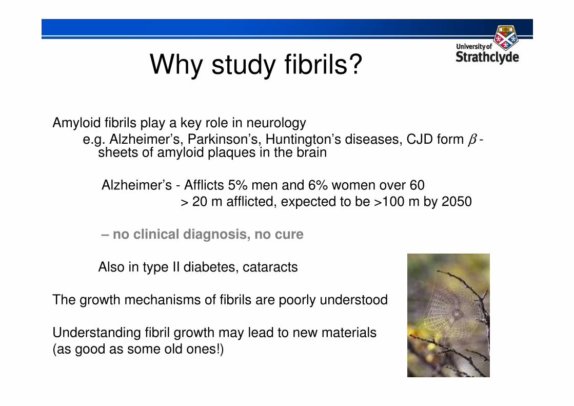
Why study fibrils?

Amyloid fibrils play a key role in neurology

e.g. Alzheimer’s, Parkinson’s, Huntington’s diseases, CJD form β -sheets of amyloid plaques in the brain

Alzheimer’s - Afflicts 5% men and 6% women over 60 > 20 m afflicted, expected to be >100 m by 2050

– no clinical diagnosis, no cure

Also in type II diabetes, cataracts

The growth mechanisms of fibrils are poorly understood

Understanding fibril growth may lead to new materials (as good as some old ones!)

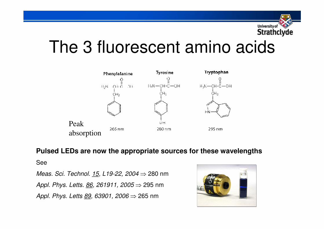
The 3 fluorescent amino acids

Pulsed LEDs are now the appropriate sources for these wavelengths

See

Meas. Sci. Technol. 15, L19-22, 2004 ⇒ 280 nm

Appl. Phys. Letts. 86, 261911, 2005 ⇒ 295 nm

Appl. Phys. Letts 89, 63901, 2006 ⇒ 265 nm

Peak

absorption

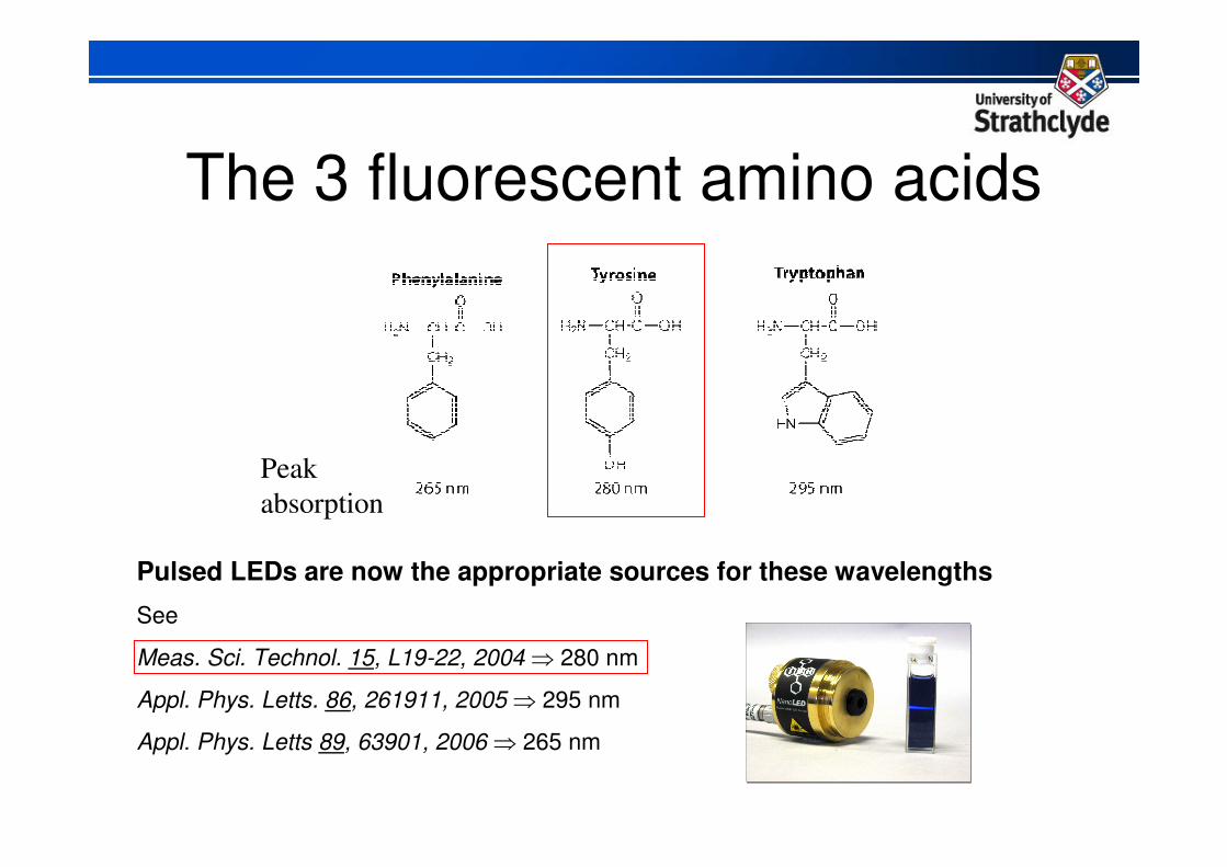
The 3 fluorescent amino acids

Pulsed LEDs are now the appropriate sources for these wavelengths

See

Meas. Sci. Technol. 15, L19-22, 2004 ⇒ 280 nm

Appl. Phys. Letts. 86, 261911, 2005 ⇒ 295 nm

Appl. Phys. Letts 89, 63901, 2006 ⇒ 265 nm

Peak

absorption

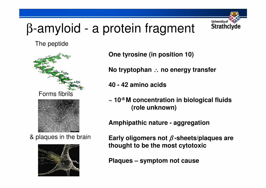
β-amyloid - a protein fragmentThe peptide

One tyrosine (in position 10)

No tryptophan ∴∴∴∴ no energy transfer

40 - 42 amino acids

~ 10-8 M concentration in biological fluids(role unknown)

Amphipathic nature - aggregation

Early oligomers not ββββ -sheets/plaques are thought to be the most cytotoxic

Plaques – symptom not cause

Forms fibrils

& plaques in the brain

200 220 240 260 280

0

5

10

15

Flu

ore

sce

nce

Inte

nsity /

a.u

.

λ /nm

226

280

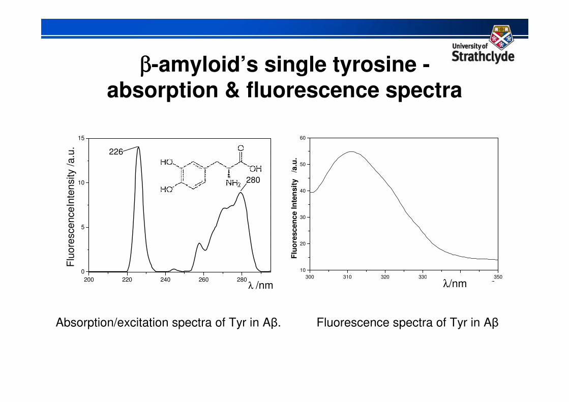
Absorption/excitation spectra of Tyr in Aβ.

ββββ-amyloid’s single tyrosine -absorption & fluorescence spectra

Fluorescence spectra of Tyr in Aβ

300 310 320 330 340 350

10

20

30

40

50

60

Tyr emission spectra

in beta-amyloid

Flu

ore

sce

nc

e I

nte

nsit

y

/a

.u.

Wavelenght /nm

Ex@279nm

λ/nm

500 550 600 6500

150

300

450

600

750

Flu

ore

scen

ce I

nte

nsity / a

.u.

λ (nm)

t / h:

341

314

247

219

80

55

29

0.8

Evolution of emission spectra of ThT in time

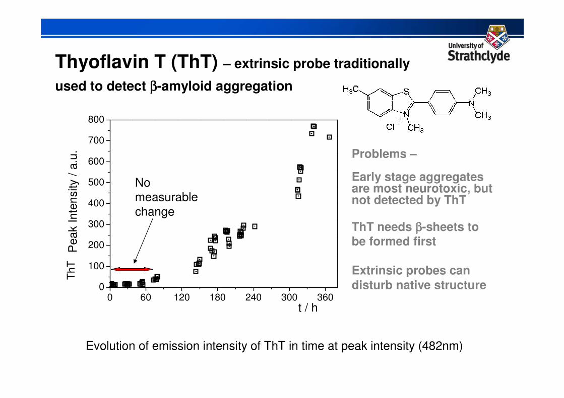
Thyoflavin T (ThT)– extrinsic probe traditionally used

to detect ββββ-amyloid aggregation

Increasingly planar configuration during

ββββ-amyloid aggregation increases fluorescence

0 60 120 180 240 300 3600

100

200

300

400

500

600

700

800

t / h

Pea

k I

nte

nsity / a

.u.

Evolution of emission intensity of ThT in time at peak intensity (482nm)

No

measurable

change

Problems –

Early stage aggregates are most neurotoxic, but not detected by ThT

ThT needs ββββ-sheets to be formed first

Extrinsic probes can

disturb native structure

Thyoflavin T (ThT) – extrinsic probe traditionally

used to detect ββββ-amyloid aggregationT

hT

0 50 100 150 200 250 300 3500

2

4

6

8

τ3

τ2

τ

/ n

sτ

1

t / h

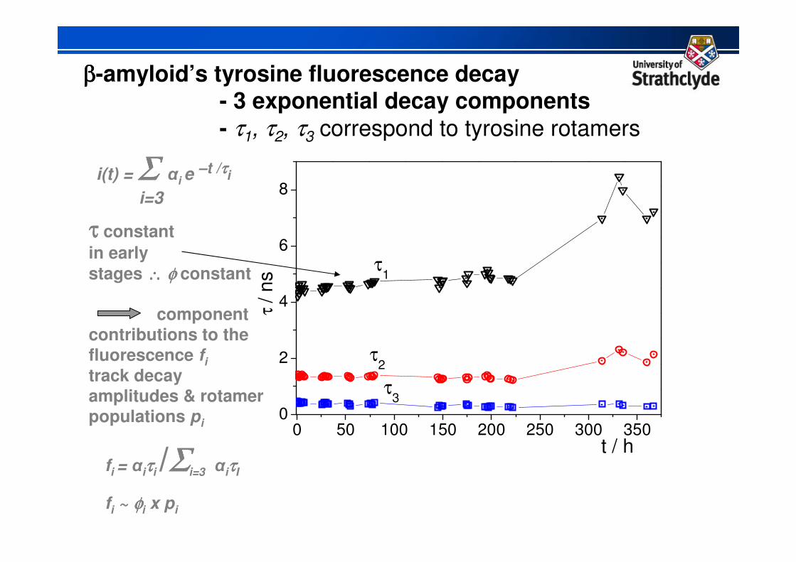
ββββ-amyloid’s tyrosine fluorescence decay- 3 exponential decay components

- τ1, τ2, τ3 correspond to tyrosine rotamers

ττττ constant

in early

stages ∴∴∴∴ φφφφ constant

componentcontributions to the fluorescence fi

track decayamplitudes & rotamerpopulations pi

i(t) = ΣΣΣΣ αi e –t /ττττi

i=3

fi = αiττττi /ΣΣΣΣi=3 αiττττI

fi ~ φφφφi x pi

0 50 100 150 200 250 300 3500.0

0.1

0.2

0.3

0.4

0.5

0.6

0.7

p3

p2

p1p

i

t / h

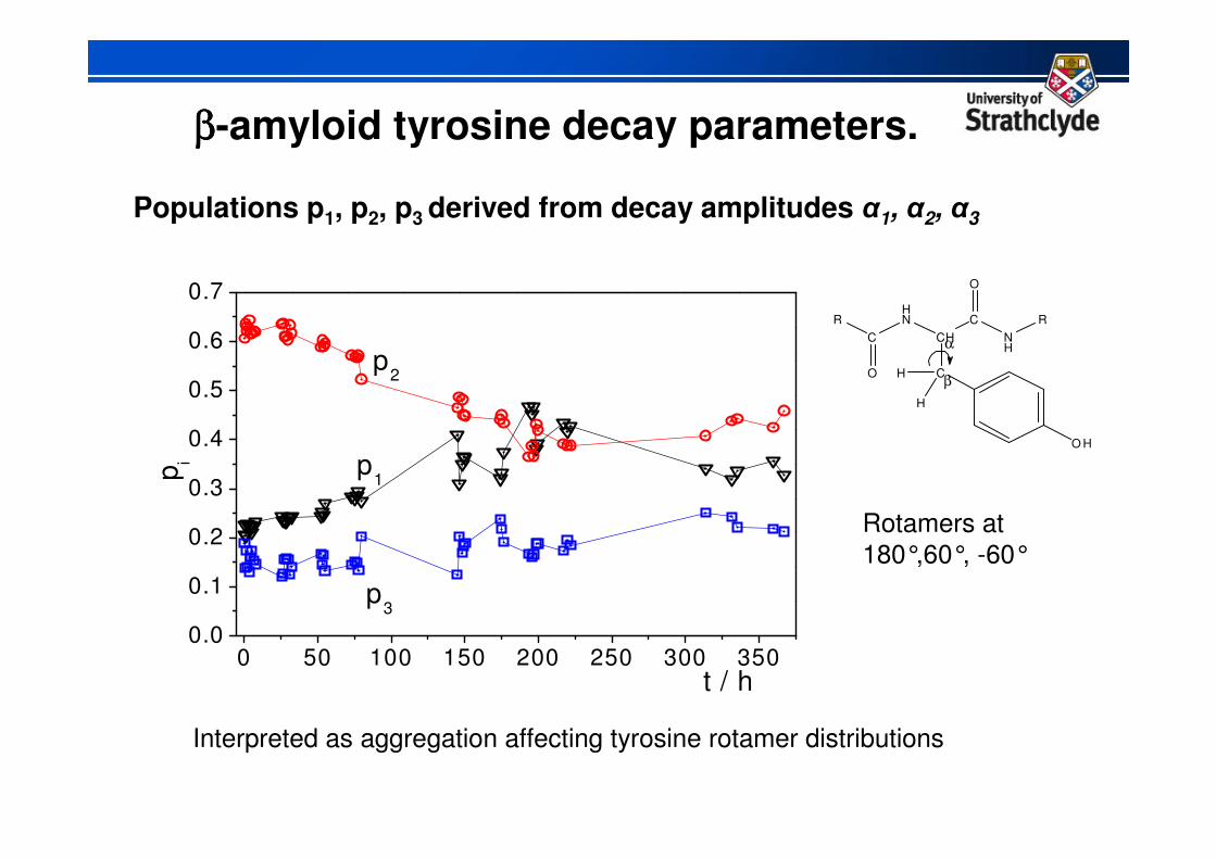
ββββ-amyloid tyrosine decay parameters.

Populations p1, p2, p3 derived from decay amplitudes α1, α2, α3

Interpreted as aggregation affecting tyrosine rotamer distributions

HN

CH

C

C

NH

O

R

C

O

R

O H

H

H

α

β

Rotamers at

180°,60°, -60°

0 15 30 45 60

0.30

0.35

0.40

0.45

p1 / p

2

t / h

1

2

3

4

Ft /

Fo

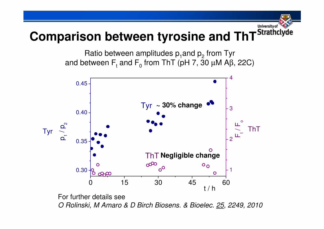
Ratio between amplitudes p1and p2 from Tyr

and between Ft and F0 from ThT (pH 7, 30 µM Aβ, 22C)

Comparison between tyrosine and ThT

~ 30% change

Tyr ThT

For further details see

O Rolinski, M Amaro & D Birch Biosens. & Bioelec. 25, 2249, 2010

Negligible change

Tyr

ThT

ββββ-Amyloid fibrils summary

Tyrosine fluorescence lifetime reports on early oligomer

aggregation -

Offers a new approach for research into drug

intervention therapeutics

3rd application - nanoparticle metrology

Concerns over possible nanoparticle toxicology and risk

to the environment

Fear of the unknown – the next asbestos?

Risks unknown

Correlation of effect with size unknown

Size often unknown

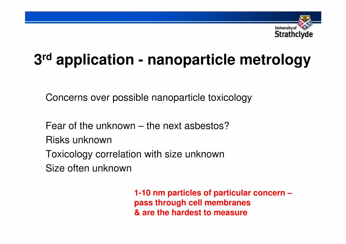
3rd application - nanoparticle metrology

Concerns over possible nanoparticle toxicology

Fear of the unknown – the next asbestos?

Risks unknown

Toxicology correlation with size unknown

Size often unknown

1-10 nm particles of particular concern –pass through cell membranes & are the hardest to measure

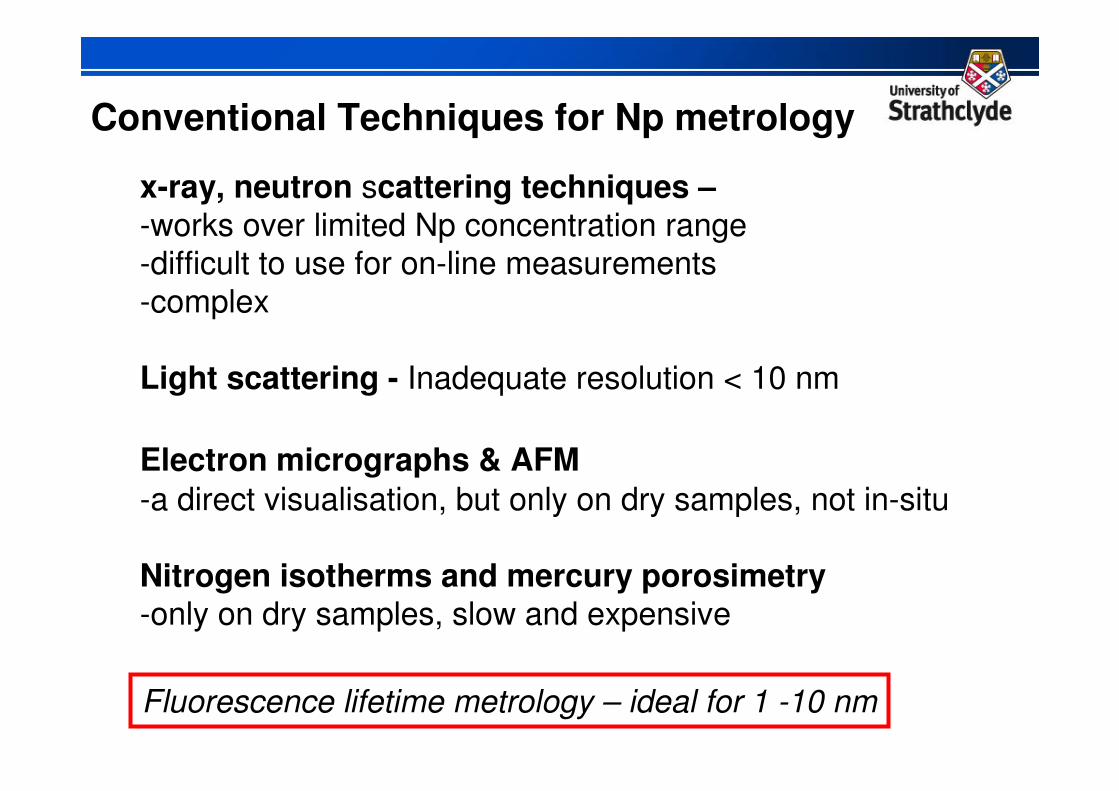
Conventional Techniques for Np metrology

x-ray, neutron scattering techniques –-works over limited Np concentration range-difficult to use for on-line measurements

-complex

Light scattering - Inadequate resolution < 10 nm

Electron micrographs & AFM

-a direct visualisation, but only on dry samples, not in-situ

Nitrogen isotherms and mercury porosimetry-only on dry samples, slow and expensive

Fluorescence lifetime metrology – ideal for 1 -10 nm

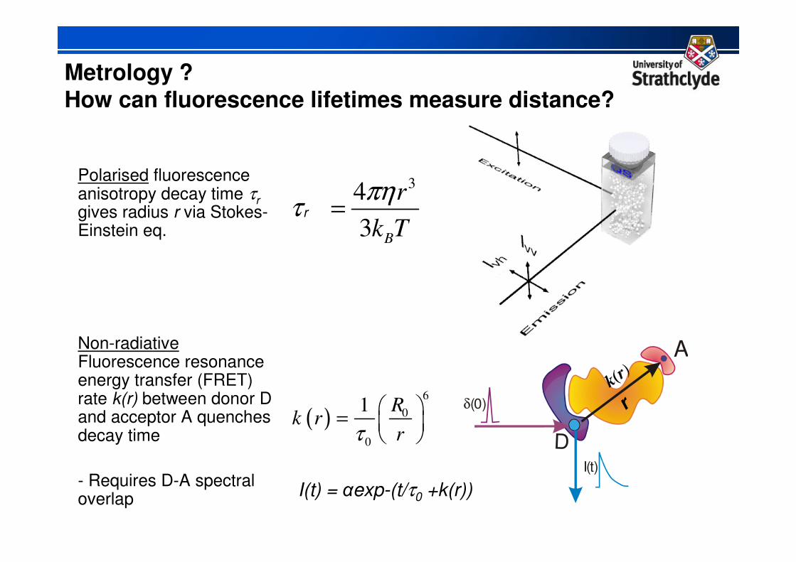
Metrology ?How can fluorescence lifetimes measure distance?

Polarised fluorescence anisotropy decay time τrgives radius r via Stokes-Einstein eq.

Non-radiativeFluorescence resonance energy transfer (FRET) rate k(r) between donor D and acceptor A quenches decay time

- Requires D-A spectral overlap

( )τ

=

6

0

0

1 Rk r

r D

A

δ(0)

I(t)

k(r)

34

3rot

B

r

k T

πητ =r

r

I(t) = αexp-(t/τ0 +k(r))

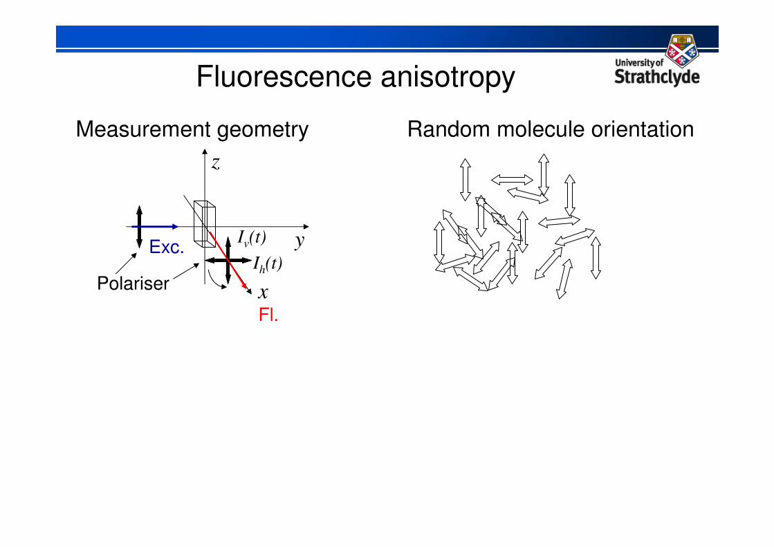
Measurement geometry Random molecule orientation

Iv(t)

Ih(t)

x

y

z

Polariser

Fluorescence anisotropy

Exc.

Fl.

Iv(t)

Ih(t)

x

y

z

Anisotropy introduced

Abs. probability ~ cos2θ

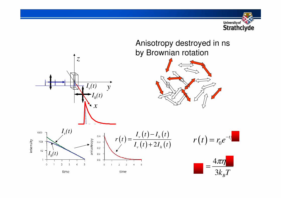
Iv(t)

Ih(t)

x

y

z

Anisotropy destroyed in ns by Brownian rotation

( )( ) ( )

( ) ( )2

v h

v h

I t I tr t

I t I t

−=

+

Ih(t)

Iv(t)

( ) 0rott

r t r eτ−=

34

3rot

B

r

k T

πητ =

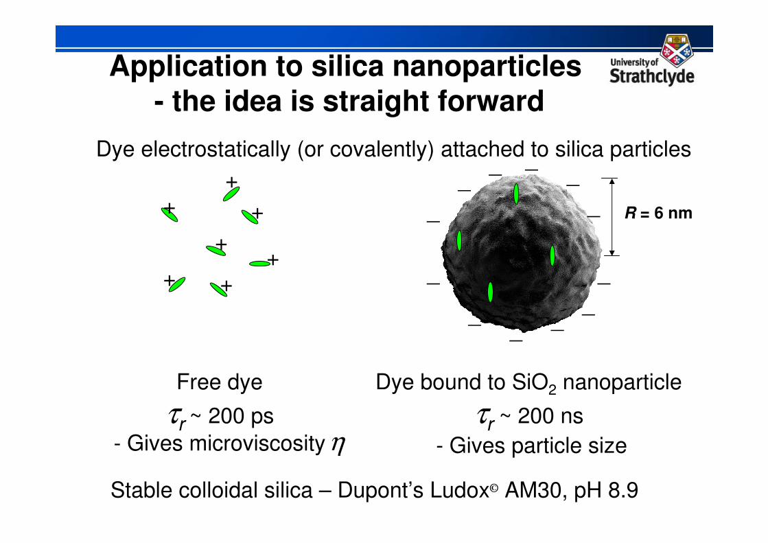
Application to silica nanoparticles- the idea is straight forward

Free dye

τr ~ 200 ps

- Gives microviscosity

Dye bound to SiO2 nanoparticle

τr ~ 200 ns

R = 6 nm

Dye electrostatically (or covalently) attached to silica particles

Stable colloidal silica – Dupont’s Ludox© AM30, pH 8.9

+

++

+

+

+

+

_

_

_ _

___

_

_

_

_

_

η - Gives particle size

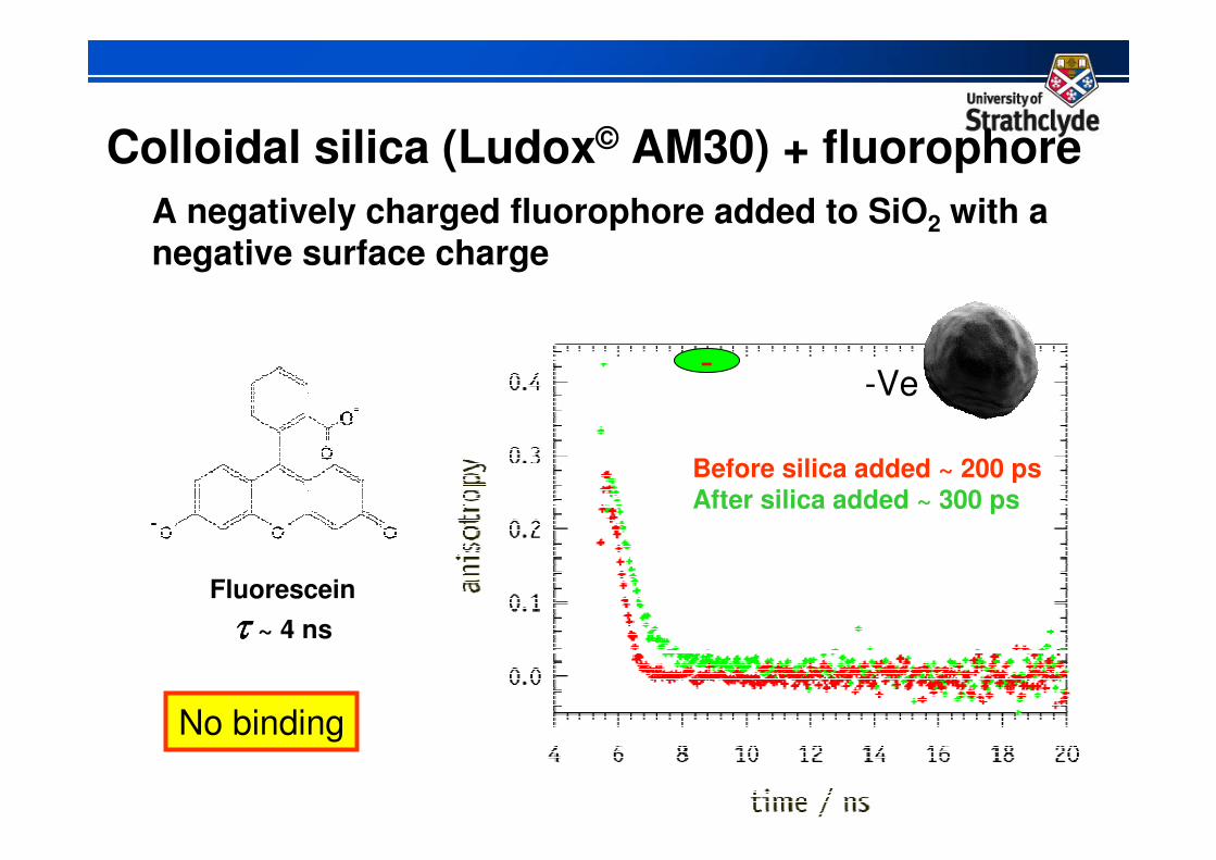
Colloidal silica (Ludox© AM30) + fluorophore

A negatively charged fluorophore added to SiO2 with a negative surface charge

Fluorescein

ττττ ~ 4 ns

No binding

Before silica added ~ 200 psAfter silica added ~ 300 ps

--Ve

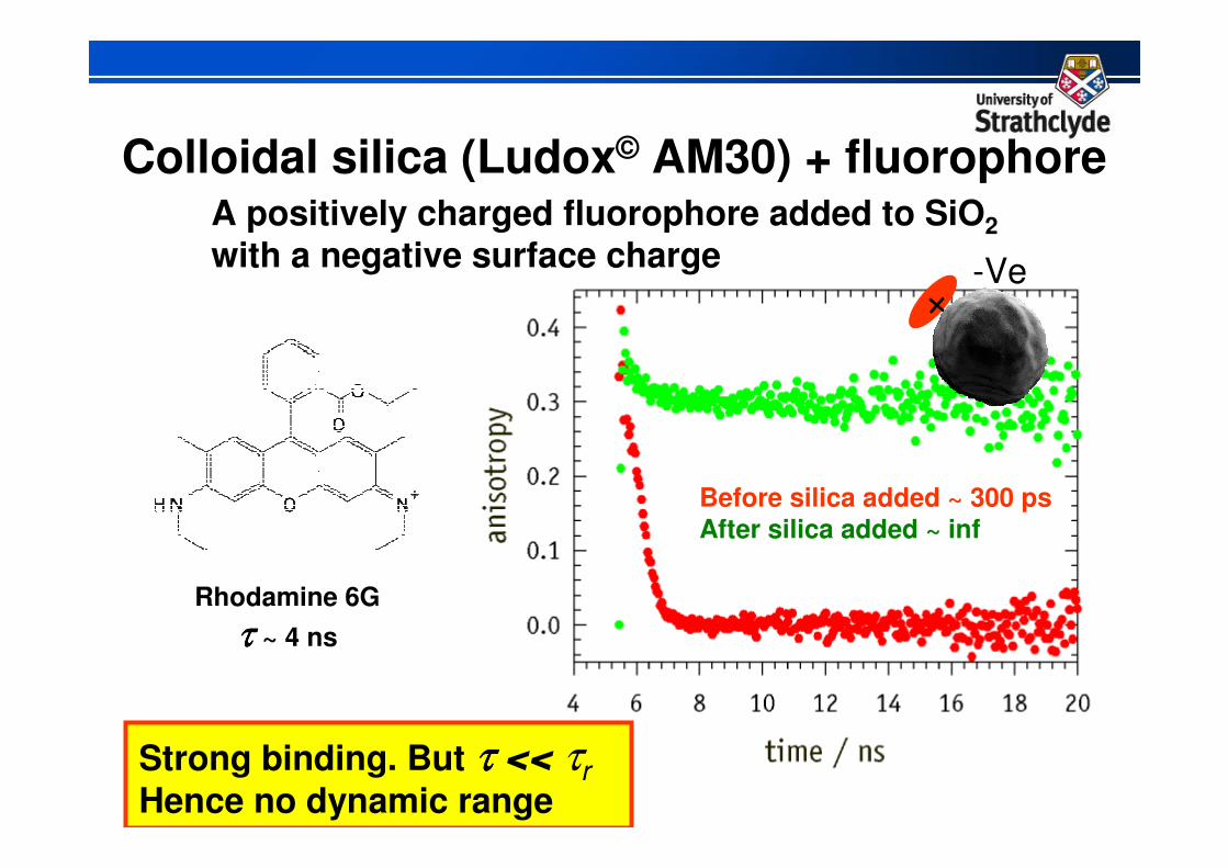
Colloidal silica (Ludox© AM30) + fluorophoreA positively charged fluorophore added to SiO2

with a negative surface charge

Rhodamine 6G

ττττ ~ 4 ns

Before silica added ~ 300 psAfter silica added ~ inf

+

Strong binding. But ττττ << τrHence no dynamic range

-Ve

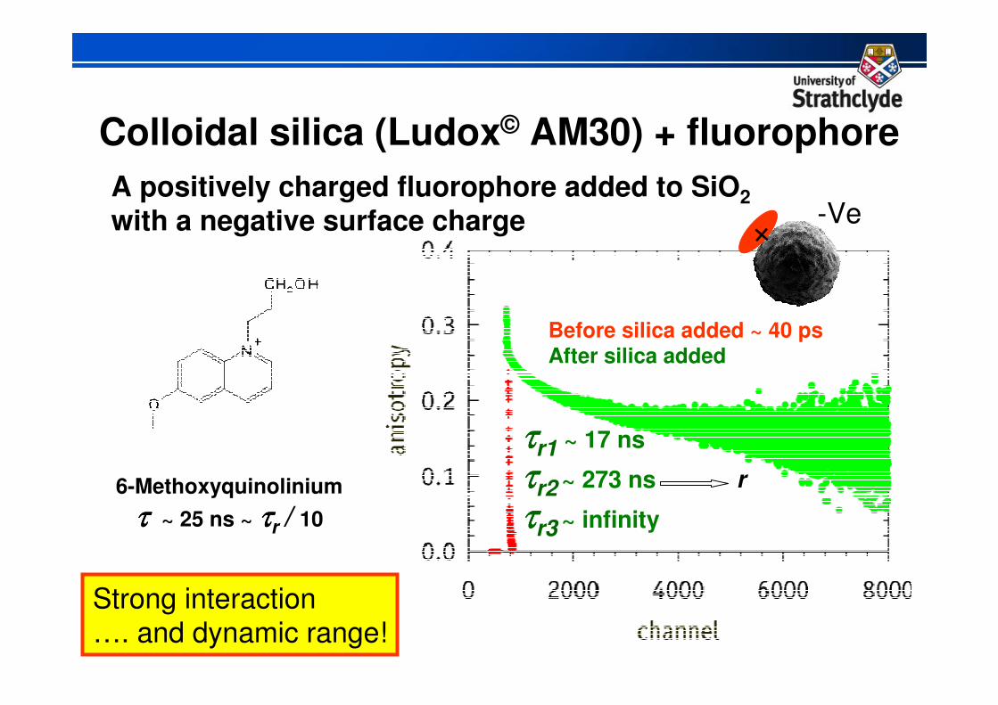
Colloidal silica (Ludox© AM30) + fluorophore

A positively charged fluorophore added to SiO2

with a negative surface charge

6-Methoxyquinolinium

ττττ ~ 25 ns ~ ττττr / 10

Before silica added ~ 40 psAfter silica added

+

Strong interaction…. and dynamic range!

-Ve

ττττr1 ~ 17 ns

ττττr2 ~ 273 ns

ττττr3 ~ infinity

r

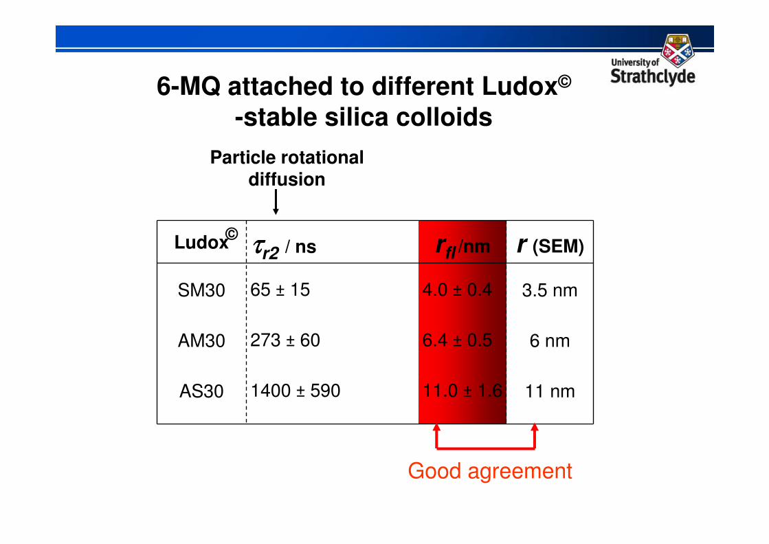
Ludox ττττr2 / ns rfl /nm r (SEM)

SM30 65 ± 15 4.0 ± 0.4 3.5 nm

AM30 273 ± 60 6.4 ± 0.5 6 nm

AS30 1400 ± 590 11.0 ± 1.6 11 nm

6-MQ attached to different Ludox©

-stable silica colloids

Particle rotationaldiffusion

Good agreement

©

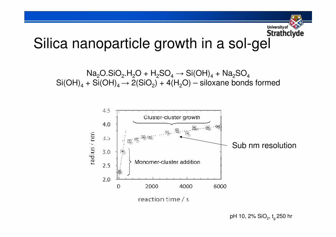
Silica nanoparticle growth in a sol-gel

Na2O.SiO2.H2O + H2SO4 → Si(OH)4 + Na2SO4

Si(OH)4 + Si(OH)4 → 2(SiO2) + 4(H2O) – siloxane bonds formed

Sub nm resolution

pH 10, 2% SiO2, tg 250 hr

Nanoparticle summary

Fluorescence anisotropy decay reliably measures

nanoparticle size ⇒⇒⇒⇒

In situ

At comparatively low cost

With ease of use

And high resolution

See

K Apperson, J Karolin, R W Martin and D J S Birch

Meas. Sci. Technol. 20, 25310, 2009

To Conclude…. Fluorescence Lifetimes

• Routine to measure

• Provide more information than steady-state fluorimetry

e.g. kinetics processes

• Versatile probe of nano-environment

• Combine with spectroscopy, microscopy & sensors

• Providing new approaches in helping to solve global

healthcare problems

Acknowledgements

Strathclyde University:

Olaf Rolinski - FRET & Aβ

Jan Karolin – nanoparticles

Mariana Amaro - Aβ

KCL School of Medicine:

John Pickup - Glucose

& co-workers

Horiba Jobin Yvon IBH Ltd:

David McLoskey - UV LEDs

Kulwinder Sagoo- UV LEDs

Sponsors:

EPSRC

Scottish Funding Council

Wellcome Trust

& thank you for attending this Webinar