Inverse Gravimetry Problem

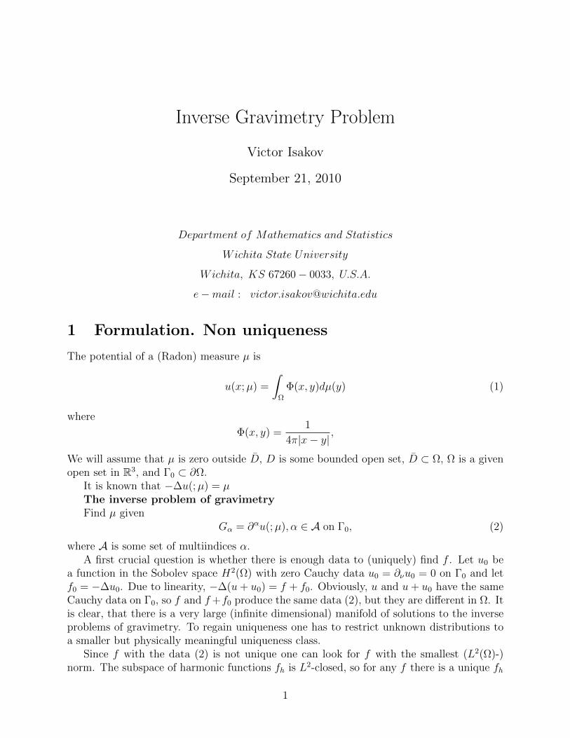
Victor Isakov

September 21, 2010

Department of Mathematics and Statistics

Wichita State University

Wichita, KS 67260− 0033, U.S.A.

e−mail : victor.isakov@wichita.edu

1 Formulation. Non uniqueness

The potential of a (Radon) measure µ is

u(x;µ) =

∫Ω

Φ(x, y)dµ(y) (1)

where

Φ(x, y) =1

4π|x− y|,

We will assume that µ is zero outside D, D is some bounded open set, D ⊂ Ω, Ω is a givenopen set in R3, and Γ0 ⊂ ∂Ω.

It is known that −∆u(;µ) = µThe inverse problem of gravimetryFind µ given

Gα = ∂αu(;µ), α ∈ A on Γ0, (2)

where A is some set of multiindices α.A first crucial question is whether there is enough data to (uniquely) find f . Let u0 be

a function in the Sobolev space H2(Ω) with zero Cauchy data u0 = ∂νu0 = 0 on Γ0 and letf0 = −∆u0. Due to linearity, −∆(u+ u0) = f + f0. Obviously, u and u+ u0 have the sameCauchy data on Γ0, so f and f+f0 produce the same data (2), but they are different in Ω. Itis clear, that there is a very large (infinite dimensional) manifold of solutions to the inverseproblems of gravimetry. To regain uniqueness one has to restrict unknown distributions toa smaller but physically meaningful uniqueness class.

Since f with the data (2) is not unique one can look for f with the smallest (L2(Ω)-)norm. The subspace of harmonic functions fh is L2-closed, so for any f there is a unique fh

1

such that f = fh + f0 where f0 is (L2)-orthogonal to fh. Since the fundamental solution isa harmonic function of y when x is outside Ω, the term f0 produces zero potential outsideΩ. Hence the harmonic orthogonal component of f has the same exterior data and minimalL2-norm. Applying the Laplacian to the both sides of the equation −∆u(; fh) = fh we arriveat the biharmonic equation ∆2u(; fh) = 0 in Ω. When Γ0 = ∂Ω we have a well-posed firstboundary value problem for the biharmonic equation for u(; fh). Solving this problem wefind from the previous Poisson equation. However, it is hard to interpret fh (geo)physicallyand knowing fh does not help much with finding f .

2 Uniqueness results

A (geo)physical intuition suggests looking for a perturbing inclusion D of constant density,i.e. for f = χD (characteristic function of an open set D).

Since (in distributional sense) −∆u(;µ) = µ in Ω, by using the Green’s formula (or thedefinition of a weak solution) we yield

−∫

Ω

u∗dµ =

∫∂Ω

((∂νu)u∗ − (∂νu∗)u) (3)

for any function u∗ ∈ H1(Ω) which is harmonic in Ω. If Γ0 = ∂Ω, then the right side in (3)is known, we are given all harmonic moments of µ. In particular, letting u∗ = 1 we obtainthe total mass of µ, and by letting u∗ to be coordinate (linear) functions we obtain momentsof µ of first order, and hence the center of gravity of µ.

Even when one assumes that f = χD, there is a non uniqueness due to possible dis-connectedness of complement of D. Indeed, it is well known that if D is the ball B(a,R)with center a of radius R then its Newtonian potential u(x,D) = M 1

4π|x−a| , where M is the

total mass of D. So the exterior potentials of all annuli B(a,R2) \ B(a,R1) are same whenR3

1 − R32 = C where C is a positive constant. Moreover, by using this simple example and

some reflections in Rn one can find two different domains with connected boundaries andequal exterior Newtonian potentials. Augmenting this construction by the condensation ofsingularities argument from the theory of functions of complex variables one can construct acontinuum of different domains with connected boundaries and same exterior potential. Sothere is a need in geometrical conditions on D.

A domain D is called star shaped with respect to a point a if any ray originated at aintersects D over an interval. An open set D is x1 convex if any straight line parallel to thex1-axis intersects D over an interval.

Theorem 2.1. Let D1, D2 be two star-shaped with respect to their centers of gravity or twox1 convex domains in Rn. Let u1, u2 be potentials of D = D1, D2.

If u1 = u2, ∂νu1 = ∂νu2 on Γ0, then D1 = D2

Returning to the uniqueness proof we assume that the are two x1-convex D1, D2 withthe same data. By uniqueness in the Cauchy problem for the Laplace equation u1 = u2 near∂Ω. Then from (3) ∫

D1

u∗ =

∫D2

u∗

2

for any function u∗ which is harmonic in Ω. The Novikov’s method of orthogonality is toassume that D1 and D2 are different, and then to select u∗ in such way that the left integralis less that the right one. To achieve this goal u∗ is replaced by its derivative, one integratesby parts to move integrals to boundaries and makes use of the maximum principles to boundinterior integrals.

Let D = x : d(x1, x3) < x2 < γ(x1, x3), be a Lipschitz domain. The unknown d ∈ Lipdescribes the shape of the floor/ice, Γ = (x1, γ(x1)), x1 ∈ Γ′ is a known upper part of ∂D,Γ0 = x : x3 = H (airborne/satellite measurements).

At present, we have the following uniqueness result.

Theorem 2.2. Let γ ∈ Lip and Γ′ be known. Then the data (2) for µ = gdΓ + χD uniquelydetermine g(thickness of snow) on Γ and D.

The exterior gravity field of a polygon (polyhedron) D develops singularities at cornerpoints of D. Indeed, ∂j∂ku(x;χD) where D is a polyhedron with corner at x0 behavesas −Clog|x − x0|, [1], section 4.1. Since these singularities are uniquely identified by theCauchy data, one has obvious uniqueness results under mild geometrical assumptions on D.Moreover use of singularities provides with constructive identification tools, based on rangetype algorithms in the harmonic continuation, using for example the operator of the singlelayer potential.

For proofs and further results on inverse problem of gravimetry we refer to work of V.Ivanov, Isakov, Prilepko [1], [5].

3 Stability

The inverse problem of potential theory is a severely (exponentially) ill-conditioned problemof the mathematical physics. The character of stability, conditional stability estimates, andregularization methods of numerical solutions of such problems are studied starting frompioneering work of Fritz John and Tikhonov in 1950-60s.

To understand degree of ill-conditioning one can consider harmonic continuation from thecircle Γ0 = x : |x| = R onto the inner circle Γ = x : |x| = ρ. By using polar coordinates(r, φ), any harmonic function decaying at infinity can be (in a stable way) approximatedby u(r, φ;M) =

∑Mm=1 umr

−meimφ. Let us define the linear operator of the continuation asA(∂r(, R)) = ∂ru(, ρ). Using the formula for u(;M), it is easy to see that the conditionnumber of the corresponding matrix is (R

ρ)M which is growing exponentially with respect to

M . If Rρ

= 10, then use of computers is only possible when M < 16, and typical practicalmeasurements errors of 0.01 allow meaningful computational results when M < 3.

The following logarithmic stability estimate holds and can be shown to be best possible.

Theorem 3.1. Let D1, D2 be two domains given in polar coordinates (r, σ) by the equations∂Dj = r = dj(σ) where |dj|2(S2) ≤ M2,

1M2

< dj, j = 1, 2. Let ε = ||u1 − u2||(1)(Γ0) +||∂ν(u1 − u2)||(0)(Γ0).

Then there is a constant C depending only on M2,Γ0 such that |d1 − d2| ≤ C(−logε)− 1C .

A proof in [1] is using some ideas from the proof of Theorem 1.1 and stability estimatesfor harmonic continuation.

3

Moreover, while it is not possible to obtain (even local) existence results, a special localexistence theorem is available [1], chapter 5. In more detail, if one assumes that u0 is apotential of some C3-domain D0, that the Cauchy data for a function u are close to theCauchy data of u0 and that, moreover, u admits harmonic continuation across ∂D0, as wellas suitable behavior at infinity, then u is a potential of a domain D which is close to D0.

Let DΓ be a domain containing D. The gravitational field u in Ω \DΓ can be uniquelyrepresented by a single layer potential. Hence the continuation problem from Γ0 onto Ω\DΓ

reduces to the linear integral equation∫Γ

g(y)∂αxK(x, y)dΓ(y) = Gα(x), x ∈ Γ0, α ∈ A. (4)

For computational purposes we replaced the integral by the finite sum arriving at the linearsystem Ag = G for unknown gj

J∑j=1

gj∂αxK(x(k), y(j)) = Gα(x(k)), x(k) ∈ Γ0, k = 1, ..., K (5)

where points y(1), ..., y(J) approximate surface Γ from inside.When Γ0 = x2 = 0 or Γ0 = x : r = R one can explicitly continue u by using the

Fourier transformation or spherical harmonics. There are no analytic results when Γ0 isa (relative small) part of ∂Ω, so we studied the problem numerically. Comparing resultsof the continuation from these data one can give recommendation for usefulness of devicesmeasuring higher order derivatives of the gravity potential.

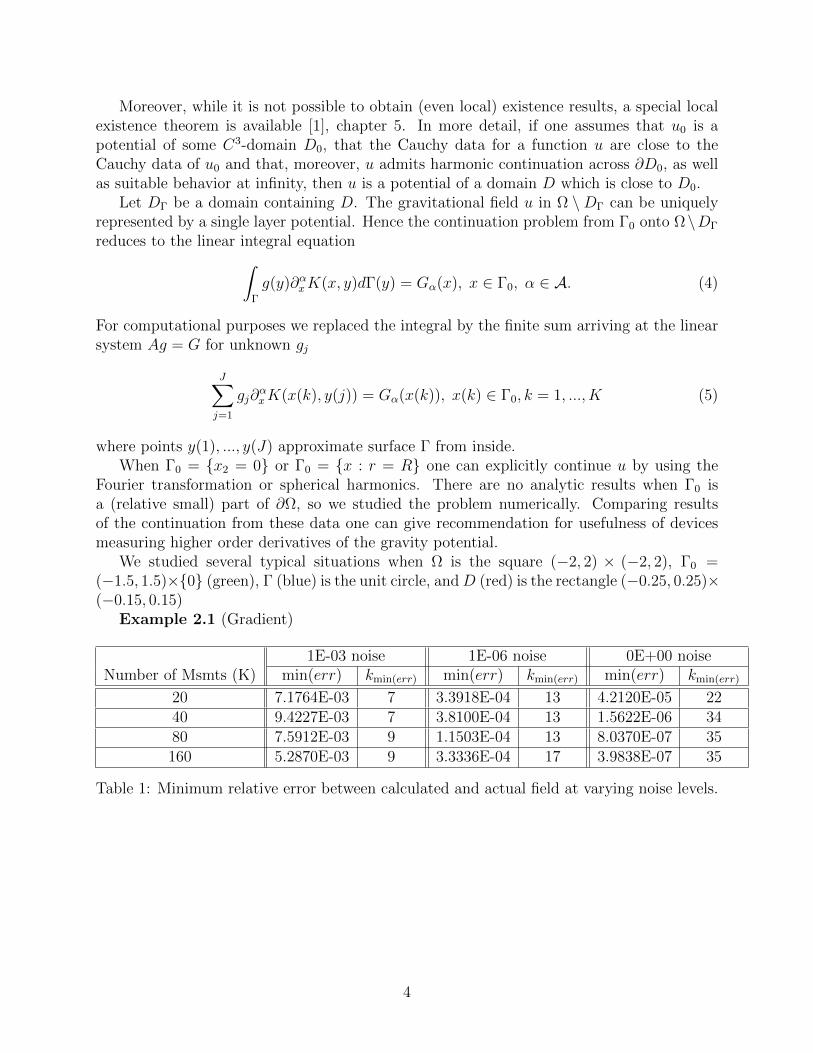
We studied several typical situations when Ω is the square (−2, 2) × (−2, 2), Γ0 =(−1.5, 1.5)×0 (green), Γ (blue) is the unit circle, andD (red) is the rectangle (−0.25, 0.25)×(−0.15, 0.15)

Example 2.1 (Gradient)

1E-03 noise 1E-06 noise 0E+00 noiseNumber of Msmts (K) min(err) kmin(err) min(err) kmin(err) min(err) kmin(err)

20 7.1764E-03 7 3.3918E-04 13 4.2120E-05 2240 9.4227E-03 7 3.8100E-04 13 1.5622E-06 3480 7.5912E-03 9 1.1503E-04 13 8.0370E-07 35160 5.2870E-03 9 3.3336E-04 17 3.9838E-07 35

Table 1: Minimum relative error between calculated and actual field at varying noise levels.

4

0 20 40 60 80 100 120 140 16010

−20

10−15

10−10

10−5

100

105

svd

(A)

Singular values of A

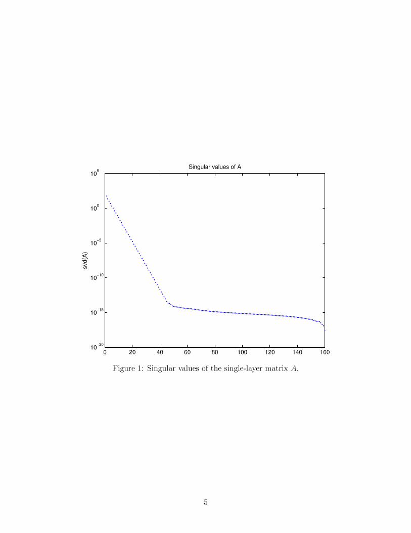
Figure 1: Singular values of the single-layer matrix A.

5

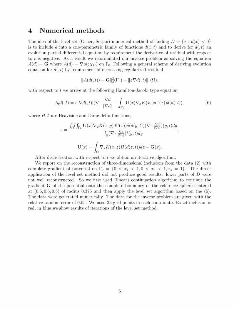
4 Numerical methods

The idea of the level set (Osher, Setjan) numerical method of finding D = x : d(x) < 0is to include d into a one-parametric family of functions d(x, t) and to derive for d(, t) anevolution partial differential equation by requirement the derivative of residual with respectto t is negative. As a result we reformulated our inverse problem as solving the equationA(d) = G where A(d) = ∇u(;χD) on Γ0. Following a general scheme of deriving evolutionequation for d(, t) by requirement of decreasing regularized residual

‖A(d(, t))−G‖22(Γ0) + ‖ε∇d(, t)‖1(Ω),

with respect to t we arrive at the following Hamilton-Jacobi type equation

∂td(, t) = ε|∇d(, t)|(∇ · ∇d|∇d|

−∫

Γ0

U(x)∇xK(x, )dΓ(x))δ(d(, t)), (6)

where H, δ are Heaviside and Dirac delta functions,

ε =

∫Ω

(∫

Γ0U(x)∇xK(x, y)dΓ(x))δ(d(y, t))(∇ · ∇d|∇d|)(y, t)dy∫

Ω(∇ · ∇d|∇d|)2(y, t)dy

,

U(x) =

∫Ω

∇xK(x, z)H(d(z, t))dz −G(x).

After discretization with respect to t we obtain an iterative algorithm.We report on the reconstruction of three-dimensional inclusions from the data (2) with

complete gradient of potential on Γ0 = 0 < x1 < 1, 0 < x3 < 1, x2 = 1. The directapplication of the level set method did not produce good results: lower parts of D werenot well reconstructed. So we first used (linear) continuation algorithm to continue thegradient G of the potential onto the complete boundary of the reference sphere centeredat (0.5, 0.5, 0.5) of radius 0.375 and then apply the level set algorithm based on the (6).The data were generated numerically. The data for the inverse problem are given with therelative random error of 0.05. We used 33 grid points in each coordinate. Exact inclusion isred, in blue we show results of iterations of the level set method.

6

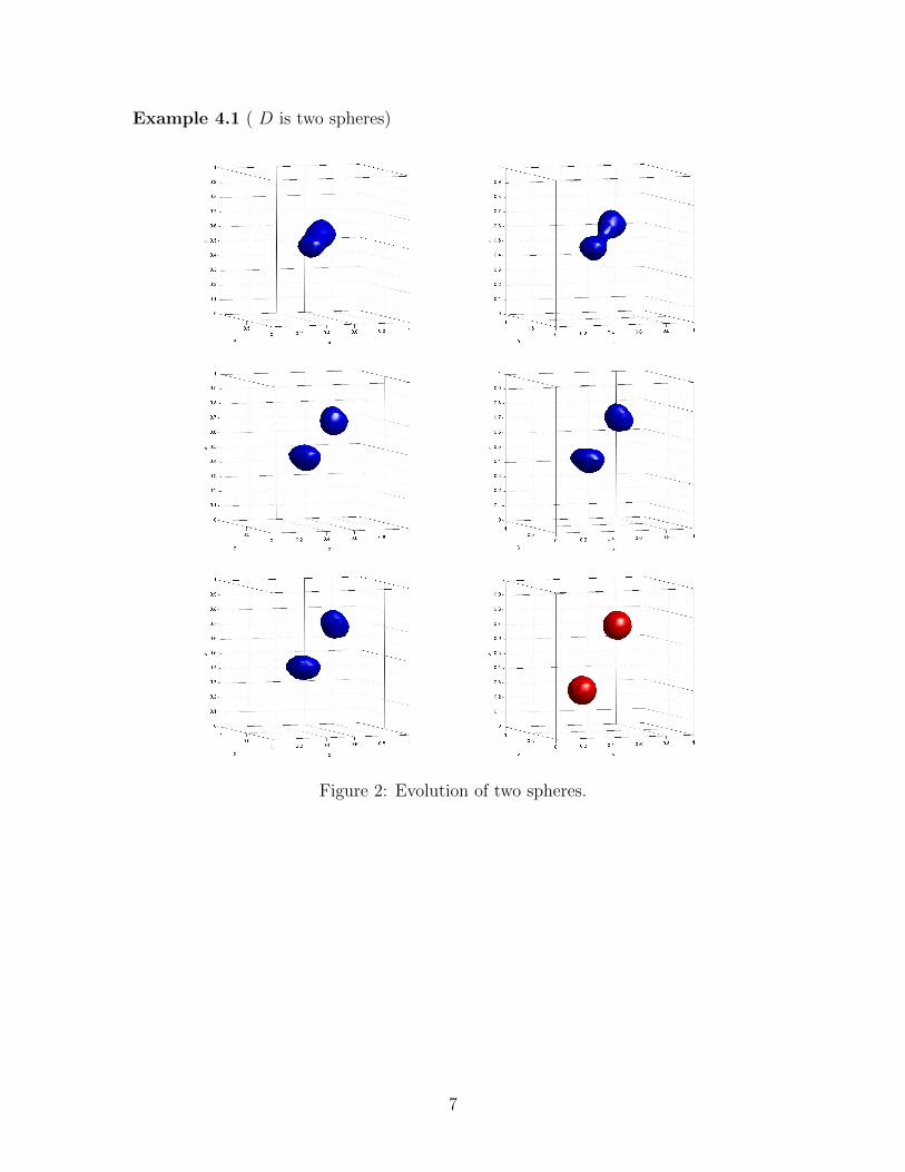
Example 4.1 ( D is two spheres)

Figure 2: Evolution of two spheres.

7

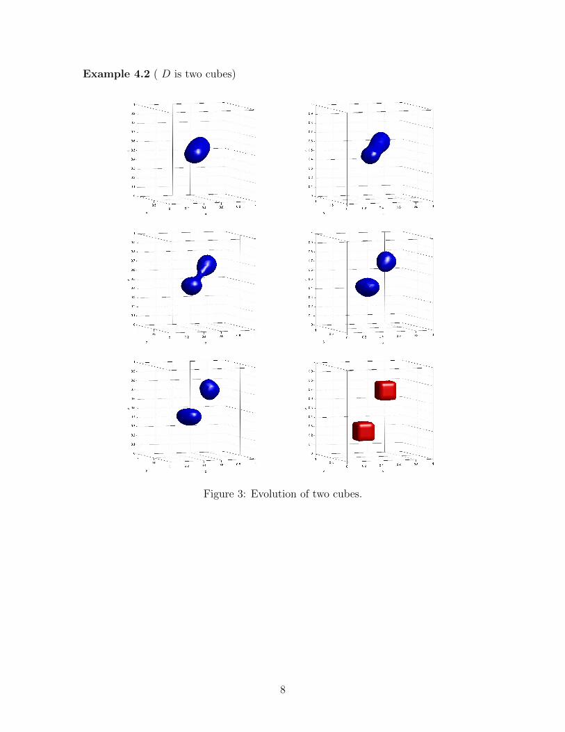
Example 4.2 ( D is two cubes)

Figure 3: Evolution of two cubes.

8

Aknowledgement:This research was in part supported by the NGA and by Emylou Keith and Betty Dutcher

Distinguished Professorship at WSU.

References

[1] V. Isakov. Inverse Source Problems, Amer. Math. Soc., Providence, RI, 1990.

[2] V. Isakov. Inverse Problems for PDE, Springer-Verlag, New York, 2006.

[3] V. Isakov, S. Leung, J. Qian, A Fast Local Level Set Method for Inverse Gravimetry,Comp. Meth. Physics, (2010) (submitted).

[4] P. Novikov. Sur le probleme inverse du potentiel, Dokl. Akad. Nauk SSSR, 18 (1938),165-168.

[5] A. I. Prilepko, D.G. Orlovskii, I. A. Vasin. Methods for solving inverse problems inmathematical physics, Marcel Dekker, New York, 2000.

9