Introductory Course on Logic and Automata Theory...
59
Introductory Course on Logic and Automata Theory Introduction to type systems [email protected] Based on slides by Jeff Foster, UMD Introduction to type systems – p. 1/5
Transcript of Introductory Course on Logic and Automata Theory...
Introductory Courseon Logic and Automata Theory
Introduction to type systems
Based on slides by Jeff Foster, UMD
Introduction to type systems – p. 1/59
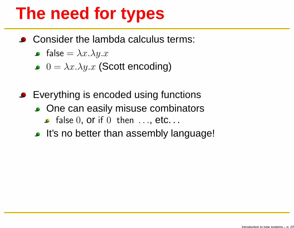
The need for typesConsider the lambda calculus terms:
false = λx.λy.x
0 = λx.λy.x (Scott encoding)
Everything is encoded using functionsOne can easily misuse combinators
false 0, or if 0 then . . ., etc. . .It’s no better than assembly language!
Introduction to type systems – p. 2/59
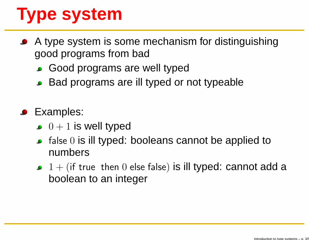
Type systemA type system is some mechanism for distinguishinggood programs from bad
Good programs are well typedBad programs are ill typed or not typeable
Examples:0 + 1 is well typedfalse 0 is ill typed: booleans cannot be applied tonumbers1 + (if true then 0 else false) is ill typed: cannot add aboolean to an integer
Introduction to type systems – p. 3/59
A definition
“A type system is a tractable syntactic method forproving the absence of certain program behaviorsby classifying phrases according to the kinds ofvalues they compute.”
– Benjamin Pierce, Types and Programming Languages
Introduction to type systems – p. 4/59
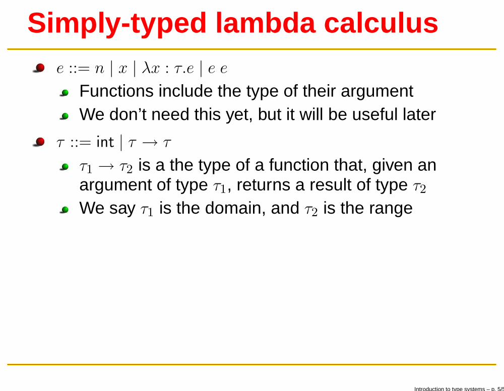
Simply-typed lambda calculuse ::= n | x | λx : τ.e | e e
Functions include the type of their argumentWe don’t need this yet, but it will be useful later
τ ::= int | τ → τ
τ1 → τ2 is a the type of a function that, given anargument of type τ1, returns a result of type τ2We say τ1 is the domain, and τ2 is the range
Introduction to type systems – p. 5/59
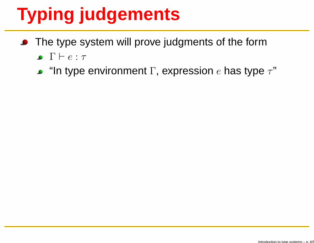
Typing judgementsThe type system will prove judgments of the form
Γ ⊢ e : τ
“In type environment Γ, expression e has type τ ”
Introduction to type systems – p. 6/59
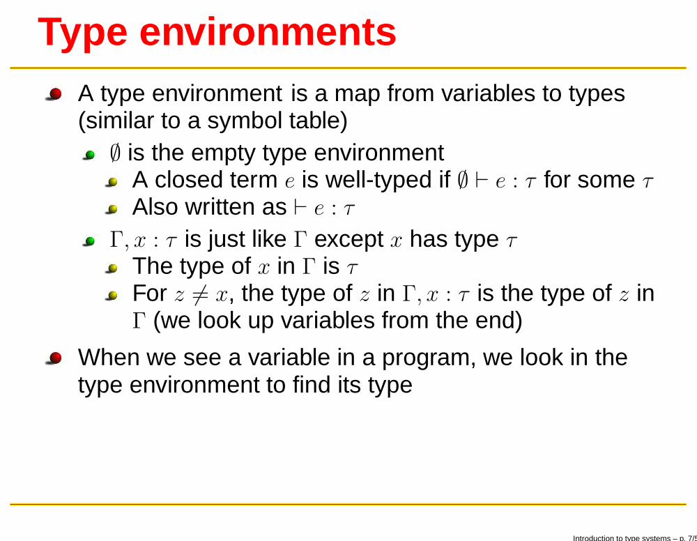
Type environmentsA type environment is a map from variables to types(similar to a symbol table)∅ is the empty type environment
A closed term e is well-typed if ∅ ⊢ e : τ for some τAlso written as ⊢ e : τ
Γ, x : τ is just like Γ except x has type τThe type of x in Γ is τFor z 6= x, the type of z in Γ, x : τ is the type of z inΓ (we look up variables from the end)
When we see a variable in a program, we look in thetype environment to find its type
Introduction to type systems – p. 7/59
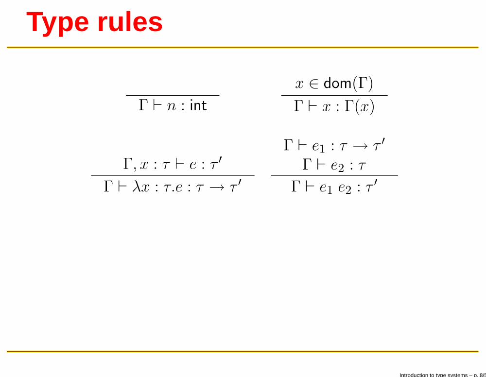
Type rules
Γ ⊢ n : int
x ∈ dom(Γ)
Γ ⊢ x : Γ(x)
Γ, x : τ ⊢ e : τ ′
Γ ⊢ λx : τ.e : τ → τ ′
Γ ⊢ e1 : τ → τ ′
Γ ⊢ e2 : τ
Γ ⊢ e1 e2 : τ ′
Introduction to type systems – p. 8/59
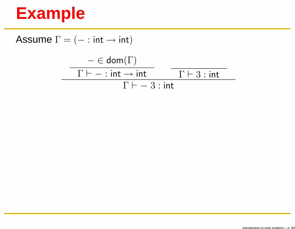
ExampleAssume Γ = (− : int→ int)
− ∈ dom(Γ)
Γ ⊢ − : int→ int Γ ⊢ 3 : intΓ ⊢ − 3 : int
Introduction to type systems – p. 9/59
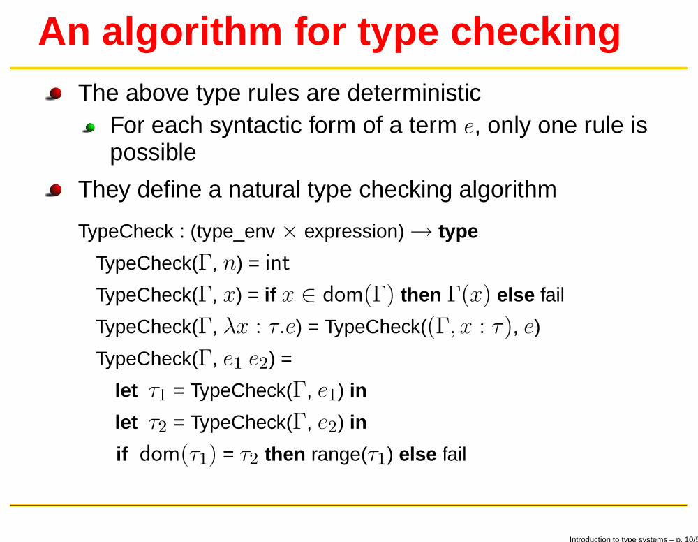
An algorithm for type checkingThe above type rules are deterministic
For each syntactic form of a term e, only one rule ispossible
They define a natural type checking algorithm
TypeCheck : (type_env × expression)→ type
TypeCheck(Γ, n) = int
TypeCheck(Γ, x) = if x ∈ dom(Γ) then Γ(x) else fail
TypeCheck(Γ, λx : τ.e) = TypeCheck((Γ, x : τ), e)
TypeCheck(Γ, e1 e2) =
let τ1 = TypeCheck(Γ, e1) in
let τ2 = TypeCheck(Γ, e2) in
if dom(τ1) = τ2 then range(τ1) else fail
Introduction to type systems – p. 10/59
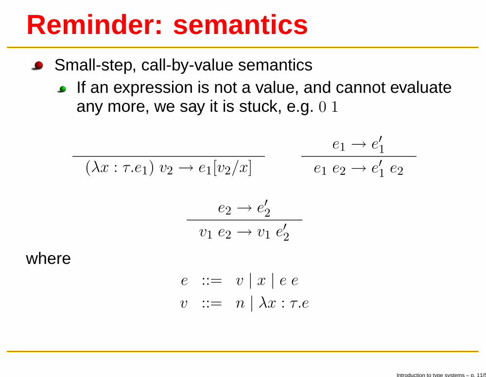
Reminder: semanticsSmall-step, call-by-value semantics
If an expression is not a value, and cannot evaluateany more, we say it is stuck, e.g. 0 1
(λx : τ.e1) v2 → e1[v2/x]
e1 → e′1e1 e2 → e′1 e2
e2 → e′2v1 e2 → v1 e
′
2
wheree ::= v | x | e e
v ::= n | λx : τ.e
Introduction to type systems – p. 11/59
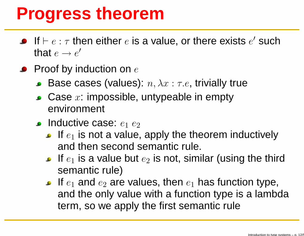
Progress theoremIf ⊢ e : τ then either e is a value, or there exists e′ suchthat e→ e′
Proof by induction on eBase cases (values): n, λx : τ.e, trivially trueCase x: impossible, untypeable in emptyenvironmentInductive case: e1 e2
If e1 is not a value, apply the theorem inductivelyand then second semantic rule.If e1 is a value but e2 is not, similar (using the thirdsemantic rule)If e1 and e2 are values, then e1 has function type,and the only value with a function type is a lambdaterm, so we apply the first semantic rule
Introduction to type systems – p. 12/59
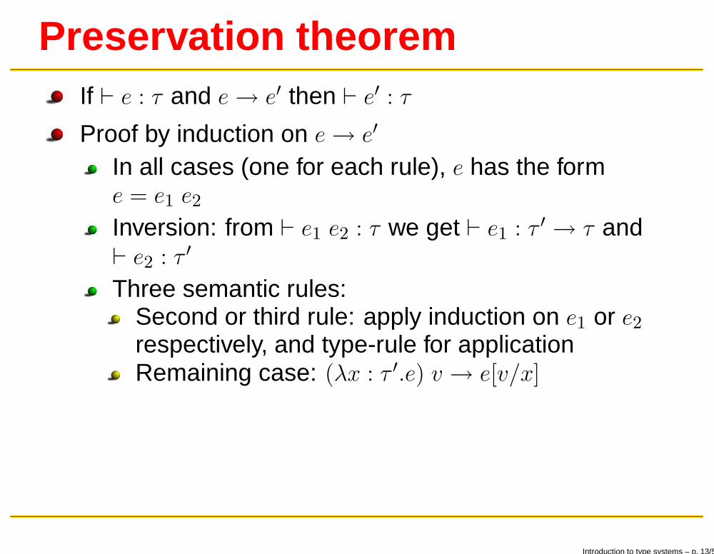
Preservation theoremIf ⊢ e : τ and e→ e′ then ⊢ e′ : τ
Proof by induction on e→ e′
In all cases (one for each rule), e has the forme = e1 e2Inversion: from ⊢ e1 e2 : τ we get ⊢ e1 : τ ′ → τ and⊢ e2 : τ ′
Three semantic rules:Second or third rule: apply induction on e1 or e2respectively, and type-rule for applicationRemaining case: (λx : τ ′.e) v → e[v/x]
Introduction to type systems – p. 13/59
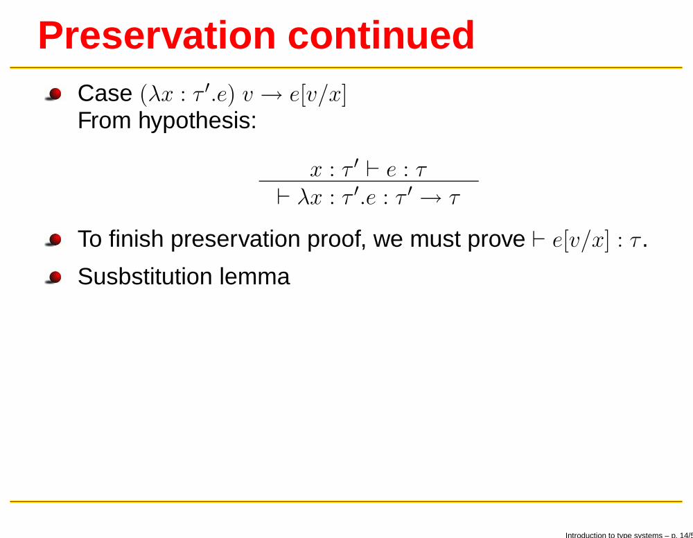
Preservation continuedCase (λx : τ ′.e) v → e[v/x]From hypothesis:
x : τ ′ ⊢ e : τ⊢ λx : τ ′.e : τ ′ → τ
To finish preservation proof, we must prove ⊢ e[v/x] : τ .
Susbstitution lemma
Introduction to type systems – p. 14/59
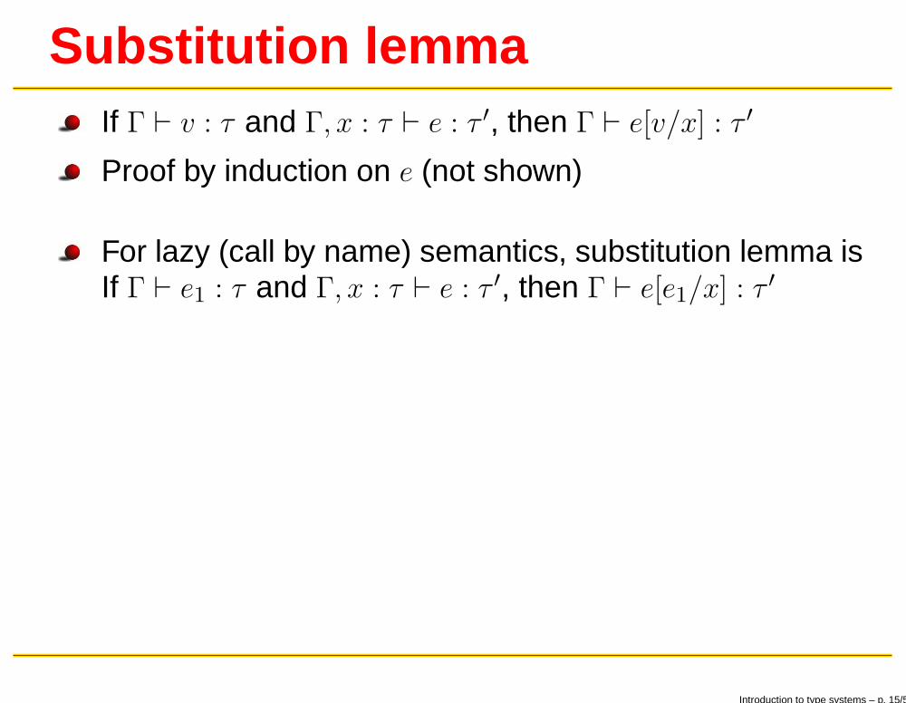
Substitution lemmaIf Γ ⊢ v : τ and Γ, x : τ ⊢ e : τ ′, then Γ ⊢ e[v/x] : τ ′
Proof by induction on e (not shown)
For lazy (call by name) semantics, substitution lemma isIf Γ ⊢ e1 : τ and Γ, x : τ ⊢ e : τ ′, then Γ ⊢ e[e1/x] : τ ′
Introduction to type systems – p. 15/59
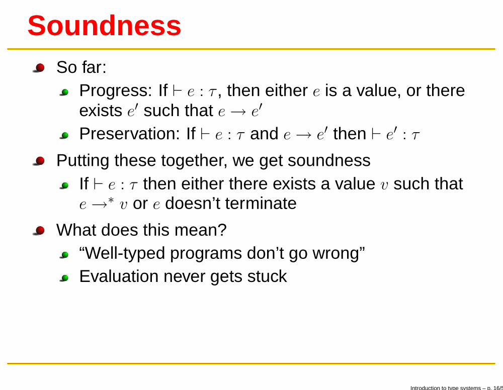
SoundnessSo far:
Progress: If ⊢ e : τ , then either e is a value, or thereexists e′ such that e→ e′
Preservation: If ⊢ e : τ and e→ e′ then ⊢ e′ : τ
Putting these together, we get soundnessIf ⊢ e : τ then either there exists a value v such thate→∗ v or e doesn’t terminate
What does this mean?“Well-typed programs don’t go wrong”Evaluation never gets stuck
Introduction to type systems – p. 16/59
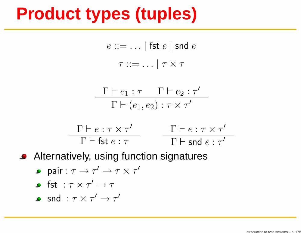
Product types (tuples)
e ::= . . . | fst e | snd e
τ ::= . . . | τ × τ
Γ ⊢ e1 : τ Γ ⊢ e2 : τ ′
Γ ⊢ (e1, e2) : τ × τ ′
Γ ⊢ e : τ × τ ′
Γ ⊢ fst e : τΓ ⊢ e : τ × τ ′
Γ ⊢ snd e : τ ′
Alternatively, using function signaturespair : τ → τ ′ → τ × τ ′
fst : τ × τ ′ → τ
snd : τ × τ ′ → τ ′
Introduction to type systems – p. 17/59
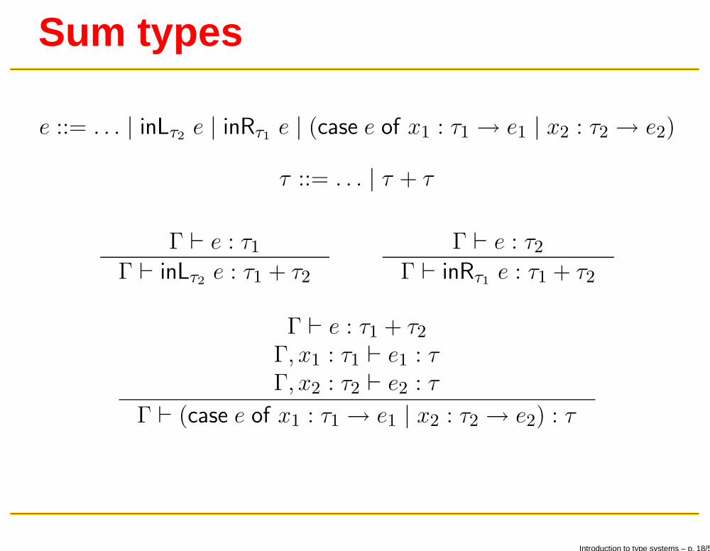
Sum types
e ::= . . . | inLτ2e | inRτ1
e | (case e of x1 : τ1 → e1 | x2 : τ2 → e2)
τ ::= . . . | τ + τ
Γ ⊢ e : τ1Γ ⊢ inLτ2
e : τ1 + τ2
Γ ⊢ e : τ2Γ ⊢ inRτ1
e : τ1 + τ2
Γ ⊢ e : τ1 + τ2Γ, x1 : τ1 ⊢ e1 : τΓ, x2 : τ2 ⊢ e2 : τ
Γ ⊢ (case e of x1 : τ1 → e1 | x2 : τ2 → e2) : τ
Introduction to type systems – p. 18/59
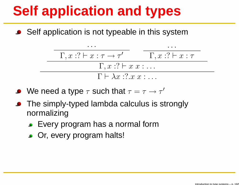
Self application and typesSelf application is not typeable in this system
· · ·Γ, x :? ⊢ x : τ → τ ′
· · ·Γ, x :? ⊢ x : τ
Γ, x :? ⊢ x x : . . .
Γ ⊢ λx :?.x x : . . .
We need a type τ such that τ = τ → τ ′
The simply-typed lambda calculus is stronglynormalizing
Every program has a normal formOr, every program halts!
Introduction to type systems – p. 19/59
Recursive typesWe can type self application if we have a type torepresent the solution to equations like τ = τ → τ ′
We define the type µα.τ to be the solution to the(recursive) equation α = τ
Example: µα.int→ α
Introduction to type systems – p. 20/59
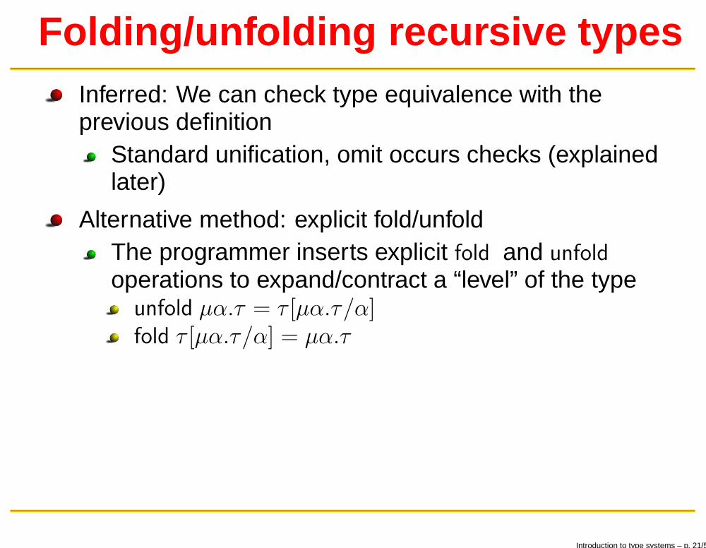
Folding/unfolding recursive typesInferred: We can check type equivalence with theprevious definition
Standard unification, omit occurs checks (explainedlater)
Alternative method: explicit fold/unfoldThe programmer inserts explicit fold and unfold
operations to expand/contract a “level” of the typeunfold µα.τ = τ [µα.τ/α]fold τ [µα.τ/α] = µα.τ
Introduction to type systems – p. 21/59
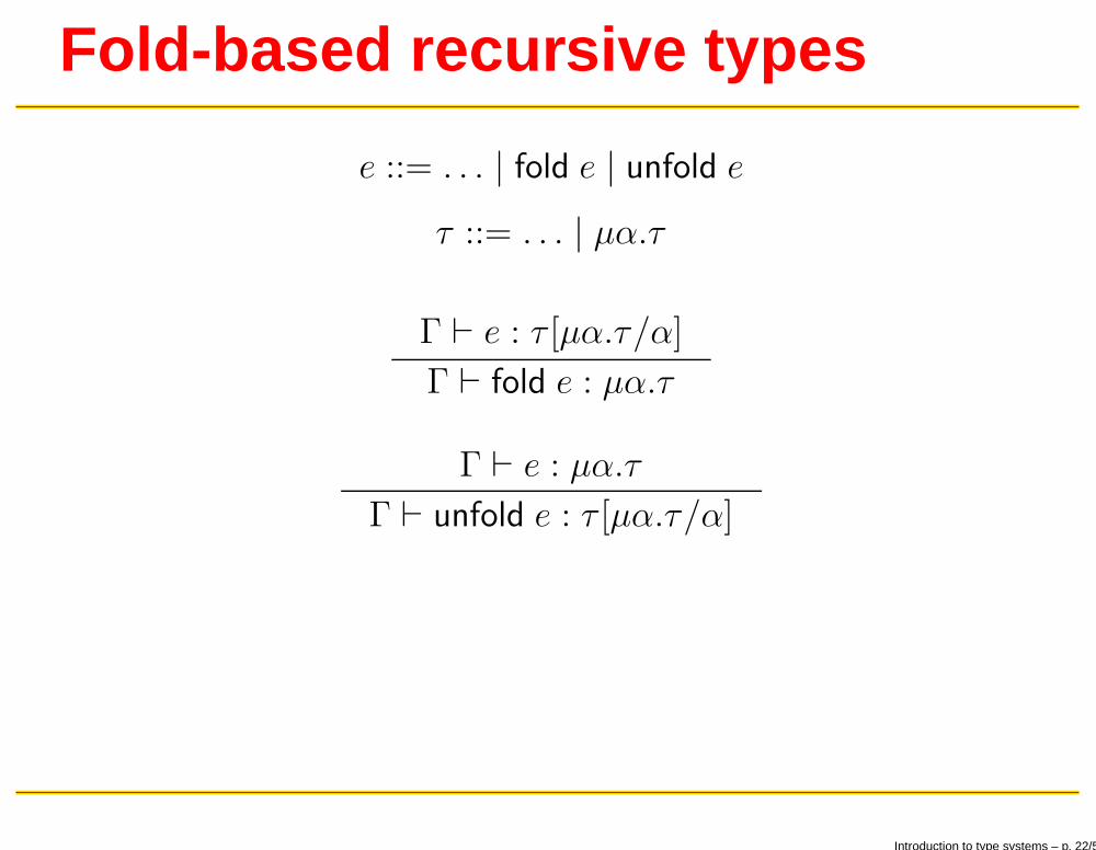
Fold-based recursive types
e ::= . . . | fold e | unfold e
τ ::= . . . | µα.τ
Γ ⊢ e : τ [µα.τ/α]
Γ ⊢ fold e : µα.τ
Γ ⊢ e : µα.τ
Γ ⊢ unfold e : τ [µα.τ/α]
Introduction to type systems – p. 22/59
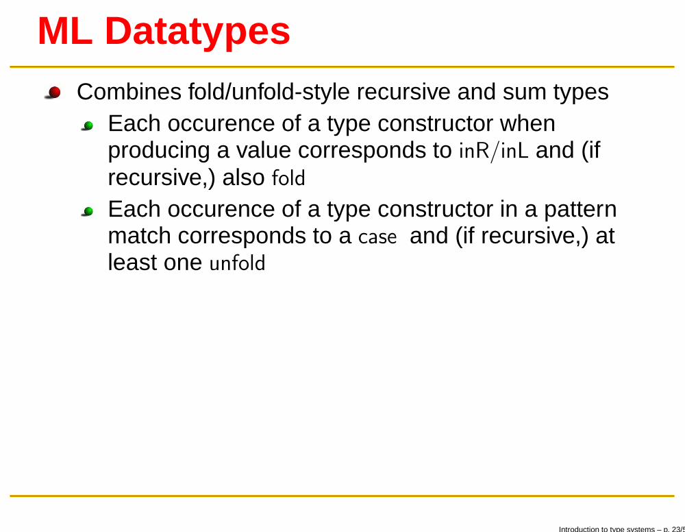
ML DatatypesCombines fold/unfold-style recursive and sum types
Each occurence of a type constructor whenproducing a value corresponds to inR/inL and (ifrecursive,) also fold
Each occurence of a type constructor in a patternmatch corresponds to a case and (if recursive,) atleast one unfold
Introduction to type systems – p. 23/59
ML Datatypes examples
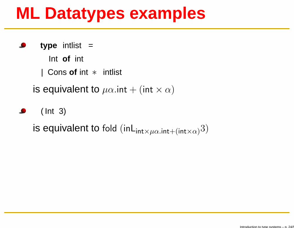
type intlist =
Int of int
| Cons of int ∗ intlist
is equivalent to µα.int + (int× α)
( Int 3)
is equivalent to fold (inLint×µα.int+(int×α)3)
Introduction to type systems – p. 24/59
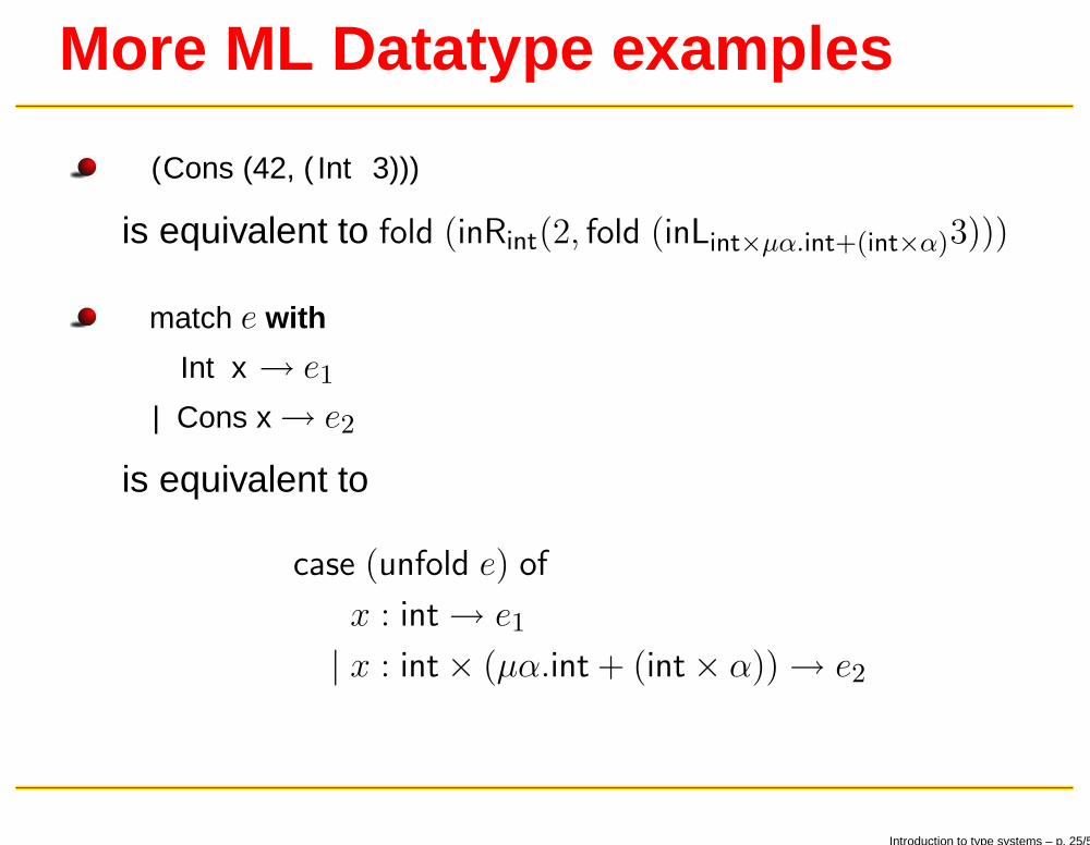
More ML Datatype examples
(Cons (42, ( Int 3)))
is equivalent to fold (inRint(2, fold (inLint×µα.int+(int×α)3)))
match e with
Int x → e1| Cons x→ e2
is equivalent to
case (unfold e) of
x : int→ e1
| x : int× (µα.int + (int× α))→ e2
Introduction to type systems – p. 25/59
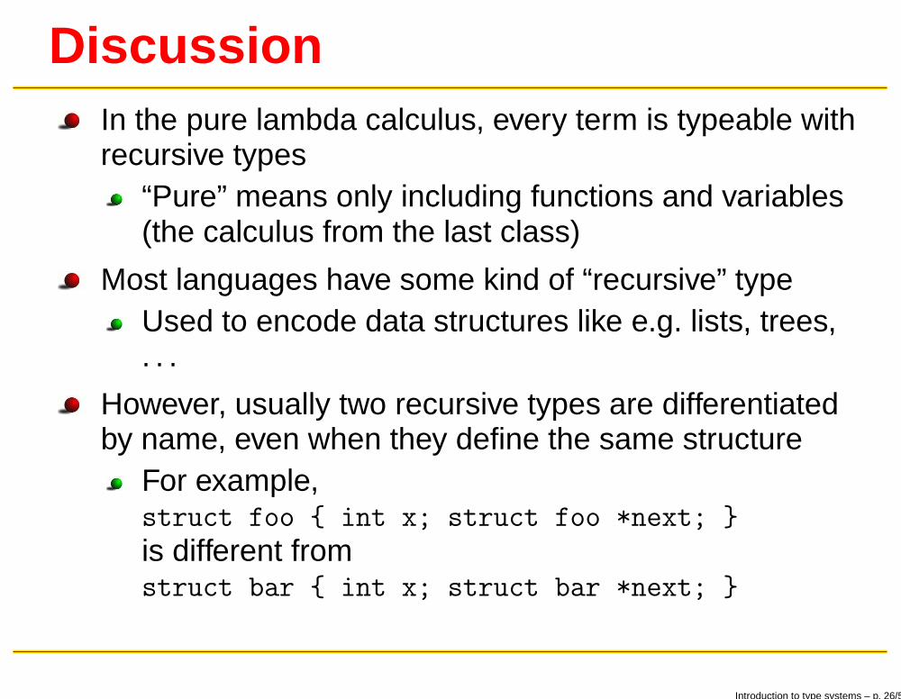
DiscussionIn the pure lambda calculus, every term is typeable withrecursive types
“Pure” means only including functions and variables(the calculus from the last class)
Most languages have some kind of “recursive” typeUsed to encode data structures like e.g. lists, trees,. . .
However, usually two recursive types are differentiatedby name, even when they define the same structure
For example,struct foo { int x; struct foo *next; }
is different fromstruct bar { int x; struct bar *next; }
Introduction to type systems – p. 26/59
Intermission
Next: Curry-Howard
correspondence
Introduction to type systems – p. 27/59

Classical propositional logicFormulas of the form
φ ::= p | ⊥ | φ ∨ φ | φ ∧ φ | φ→ φ
Where p ∈ P is an atomic proposition, e.g. “Socrates isa man”
Convenient abbreviations:¬φ means φ→ ⊥φ←→ φ′ means (φ→ φ′) ∧ (φ′ → φ)
Introduction to type systems – p. 28/59
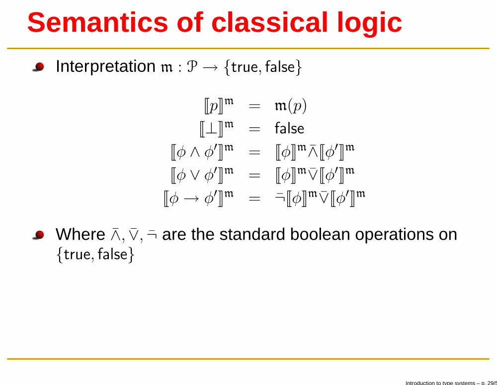
Semantics of classical logicInterpretation m : P→ {true, false}
JpKm = m(p)
J⊥Km = false
Jφ ∧ φ′Km = JφKm∧̄Jφ′Km
Jφ ∨ φ′Km = JφKm∨̄Jφ′Km
Jφ→ φ′Km = ¬̄JφKm∨̄Jφ′Km
Where ∧̄, ∨̄, ¬̄ are the standard boolean operations on{true, false}
Introduction to type systems – p. 29/59
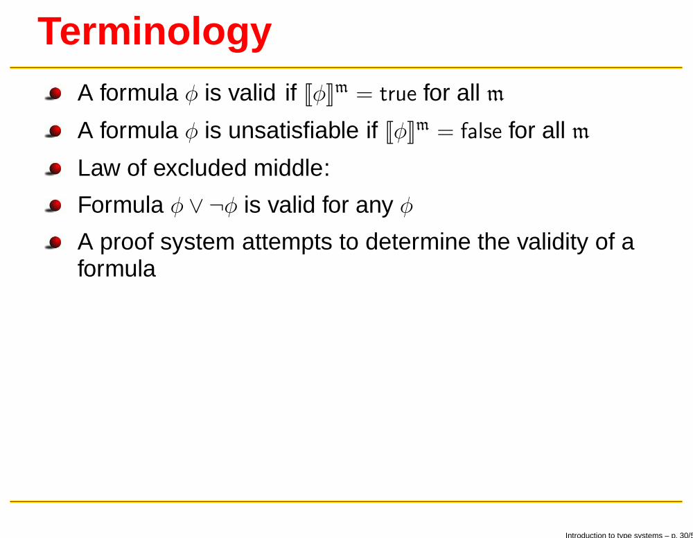
TerminologyA formula φ is valid if JφKm = true for all m
A formula φ is unsatisfiable if JφKm = false for all m
Law of excluded middle:
Formula φ ∨ ¬φ is valid for any φ
A proof system attempts to determine the validity of aformula
Introduction to type systems – p. 30/59
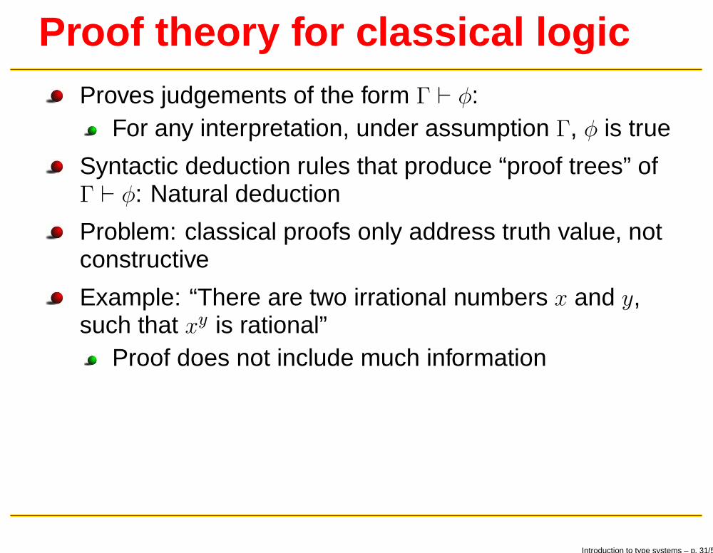
Proof theory for classical logicProves judgements of the form Γ ⊢ φ:
For any interpretation, under assumption Γ, φ is true
Syntactic deduction rules that produce “proof trees” ofΓ ⊢ φ: Natural deduction
Problem: classical proofs only address truth value, notconstructive
Example: “There are two irrational numbers x and y,such that xy is rational”
Proof does not include much information
Introduction to type systems – p. 31/59
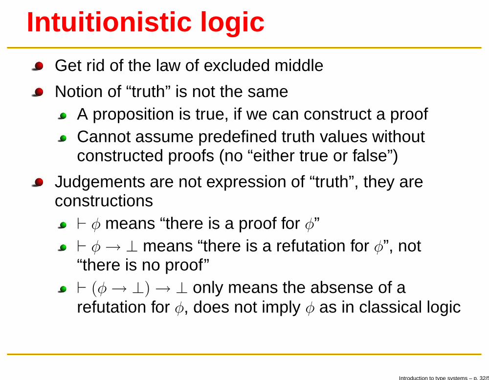
Intuitionistic logicGet rid of the law of excluded middle
Notion of “truth” is not the sameA proposition is true, if we can construct a proofCannot assume predefined truth values withoutconstructed proofs (no “either true or false”)
Judgements are not expression of “truth”, they areconstructions⊢ φ means “there is a proof for φ”⊢ φ→ ⊥ means “there is a refutation for φ”, not“there is no proof”⊢ (φ→ ⊥)→ ⊥ only means the absense of arefutation for φ, does not imply φ as in classical logic
Introduction to type systems – p. 32/59
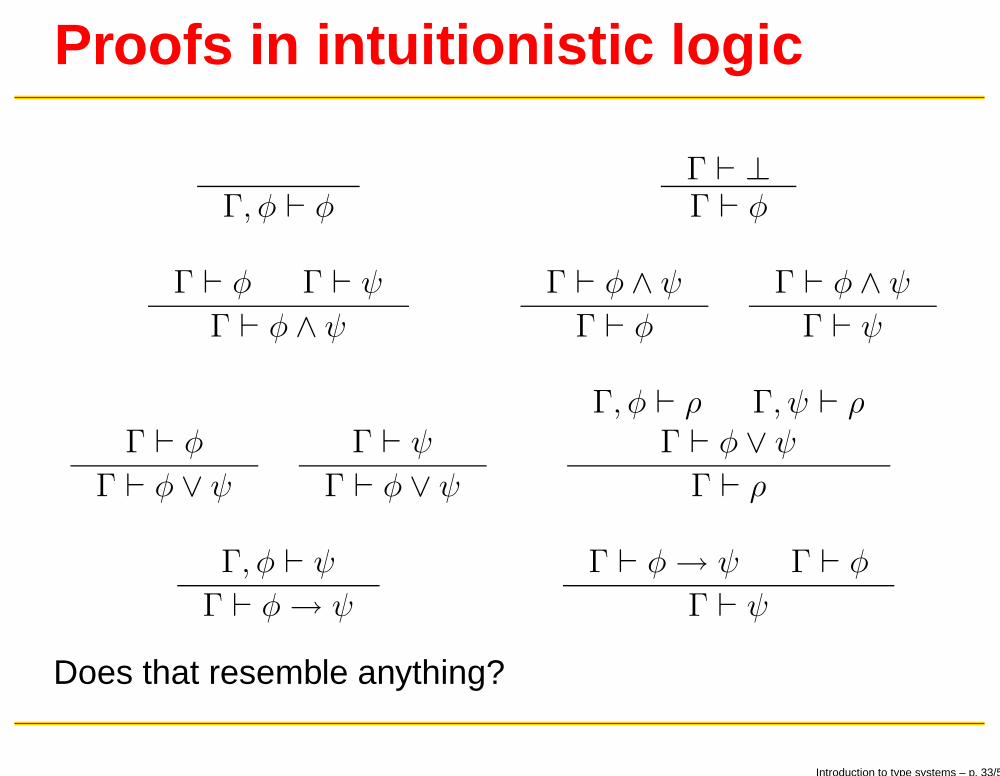
Proofs in intuitionistic logic
Γ, φ ⊢ φΓ ⊢ ⊥Γ ⊢ φ
Γ ⊢ φ Γ ⊢ ψ
Γ ⊢ φ ∧ ψ
Γ ⊢ φ ∧ ψ
Γ ⊢ φ
Γ ⊢ φ ∧ ψ
Γ ⊢ ψ
Γ ⊢ φ
Γ ⊢ φ ∨ ψ
Γ ⊢ ψ
Γ ⊢ φ ∨ ψ
Γ, φ ⊢ ρ Γ, ψ ⊢ ρΓ ⊢ φ ∨ ψ
Γ ⊢ ρ
Γ, φ ⊢ ψ
Γ ⊢ φ→ ψ
Γ ⊢ φ→ ψ Γ ⊢ φ
Γ ⊢ ψ
Does that resemble anything?
Introduction to type systems – p. 33/59
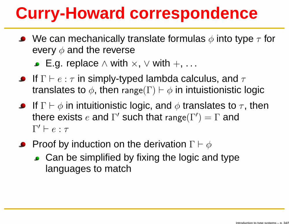
Curry-Howard correspondenceWe can mechanically translate formulas φ into type τ forevery φ and the reverse
E.g. replace ∧ with ×, ∨ with +, . . .
If Γ ⊢ e : τ in simply-typed lambda calculus, and τtranslates to φ, then range(Γ) ⊢ φ in intuistionistic logic
If Γ ⊢ φ in intuitionistic logic, and φ translates to τ , thenthere exists e and Γ′ such that range(Γ′) = Γ andΓ′ ⊢ e : τ
Proof by induction on the derivation Γ ⊢ φ
Can be simplified by fixing the logic and typelanguages to match
Introduction to type systems – p. 34/59
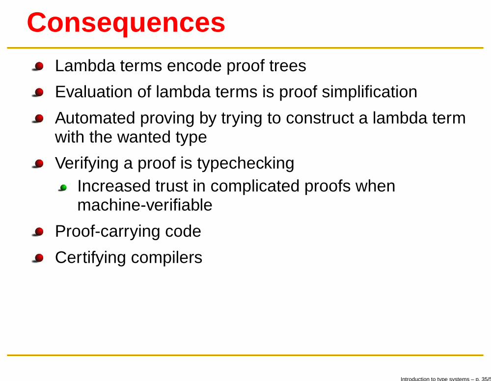
ConsequencesLambda terms encode proof trees
Evaluation of lambda terms is proof simplification
Automated proving by trying to construct a lambda termwith the wanted type
Verifying a proof is typecheckingIncreased trust in complicated proofs whenmachine-verifiable
Proof-carrying code
Certifying compilers
Introduction to type systems – p. 35/59
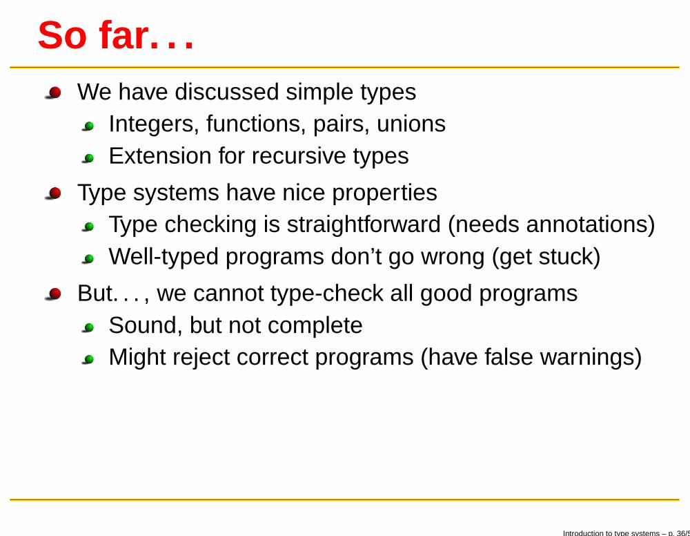
So far. . .We have discussed simple types
Integers, functions, pairs, unionsExtension for recursive types
Type systems have nice propertiesType checking is straightforward (needs annotations)Well-typed programs don’t go wrong (get stuck)
But. . . , we cannot type-check all good programsSound, but not completeMight reject correct programs (have false warnings)
Introduction to type systems – p. 36/59
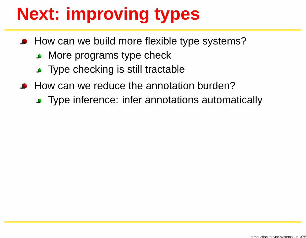
Next: improving typesHow can we build more flexible type systems?
More programs type checkType checking is still tractable
How can we reduce the annotation burden?Type inference: infer annotations automatically
Introduction to type systems – p. 37/59
Parametric polymorphismObservation: λx.x returns its argument exactly withoutany constraints on the type of x
The identity function works for any argument type
We can express this with universal quantificationλx.x : ∀α.α→ α
For any type α the identity function has type α→ α
This is also known as parametric polymorphism
Introduction to type systems – p. 38/59
System F: annotated polymorphismWe extend the previous system:
τ ::= int | τ → τ | α | ∀α.τ
e ::= n | x | λx.e | e e | Λα.e | e[τ ]
We add polymorphic types, and we add explicit typeabstraction (generalization over all α) . . .
Explicit creation of values ov polymorphic types
. . . and type application (instantiation of generalizedtypes)
Explicitly marks code locations where a value ofpolymorphic type is used
System by Girard, concurrently Reynolds
Introduction to type systems – p. 39/59
Defining polymorphic functionsPolymorphic functions map types to terms
Normal functions map terms to terms
ExamplesΛα.λx : α.x : ∀α.α→ α
Λα.Λβ.λx : α.λy : β.x : ∀α.∀β.α→ β → α
Λα.Λβ.λx : α.λy : β.y : ∀α.∀β.α→ β → β
Introduction to type systems – p. 40/59
InstantiationWhen we use a parametric polymorphic type, we applyor instantiate it with a particular type
In System F this is done by hand(Λα.λx : α.x)[τ1] : τ1 → τ1
(Λα.λx : α.x)[τ2] : τ2 → τ2
This is where the term parametric comes fromThe type ∀α.α→ α is a “function” in the domain oftypesIt is given a parameter at instantiation time
Introduction to type systems – p. 41/59
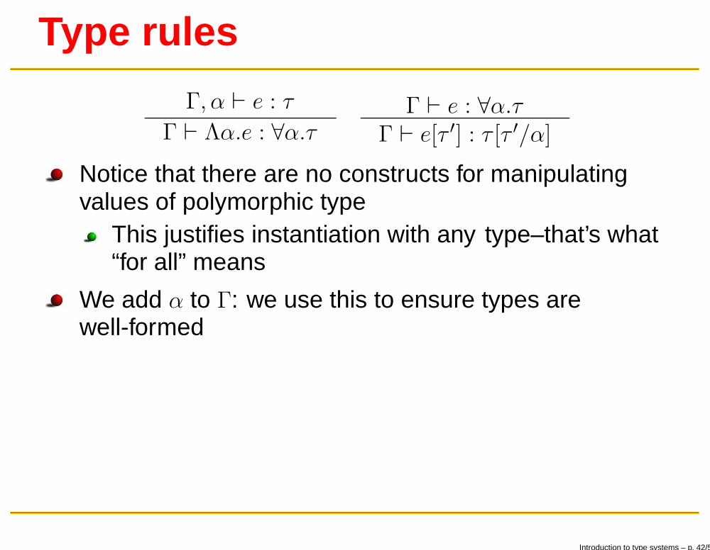
Type rules
Γ, α ⊢ e : τ
Γ ⊢ Λα.e : ∀α.τΓ ⊢ e : ∀α.τ
Γ ⊢ e[τ ′] : τ [τ ′/α]
Notice that there are no constructs for manipulatingvalues of polymorphic type
This justifies instantiation with any type–that’s what“for all” means
We add α to Γ: we use this to ensure types arewell-formed
Introduction to type systems – p. 42/59
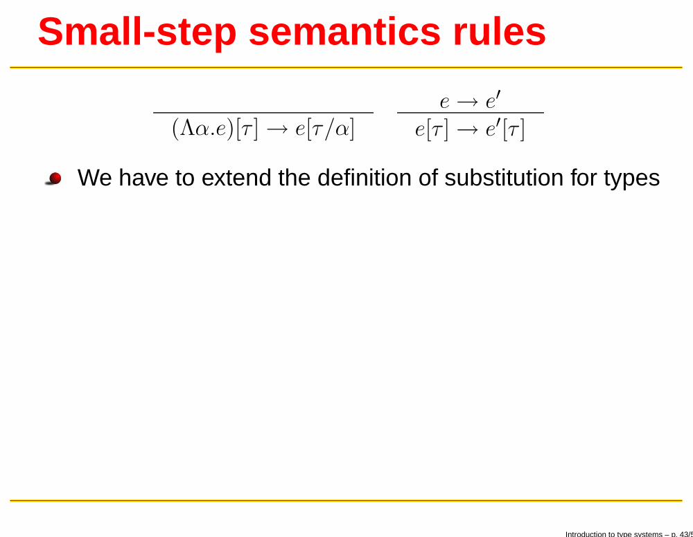
Small-step semantics rules
(Λα.e)[τ ]→ e[τ/α]e→ e′
e[τ ]→ e′[τ ]
We have to extend the definition of substitution for types
Introduction to type systems – p. 43/59
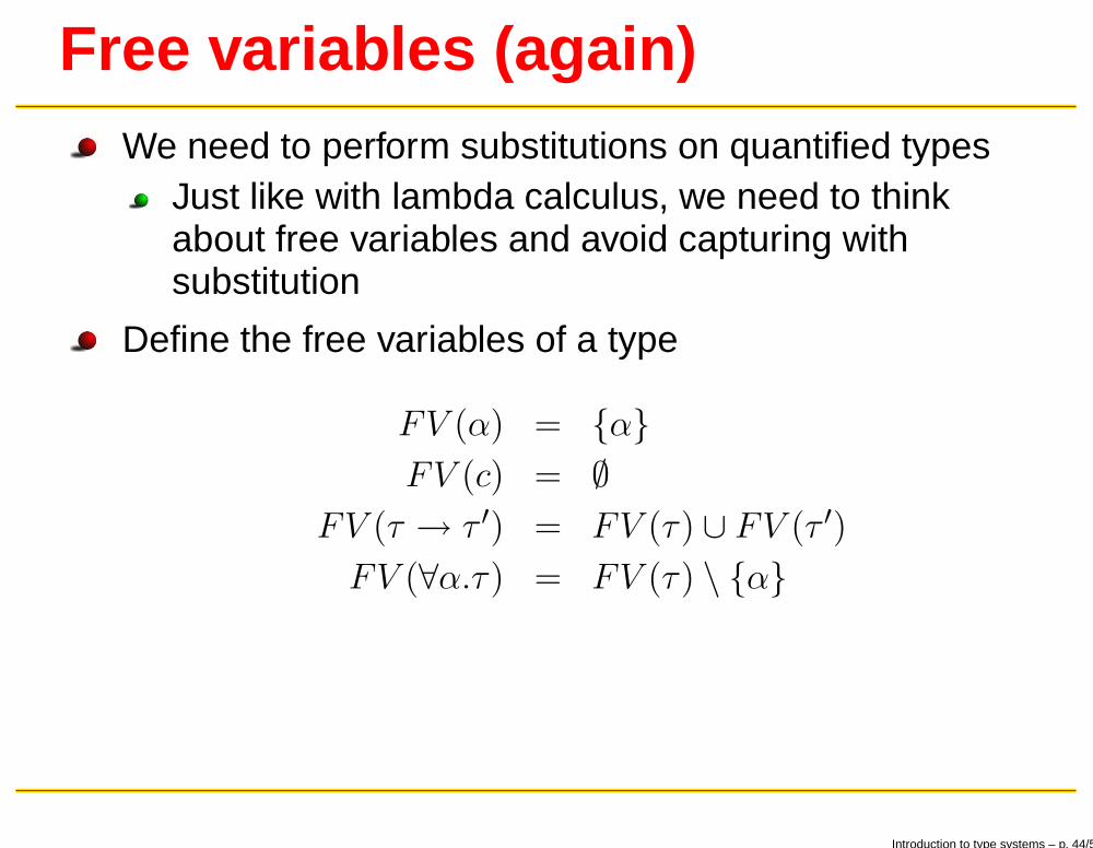
Free variables (again)We need to perform substitutions on quantified types
Just like with lambda calculus, we need to thinkabout free variables and avoid capturing withsubstitution
Define the free variables of a type
FV (α) = {α}
FV (c) = ∅
FV (τ → τ ′) = FV (τ) ∪ FV (τ ′)
FV (∀α.τ) = FV (τ) \ {α}
Introduction to type systems – p. 44/59
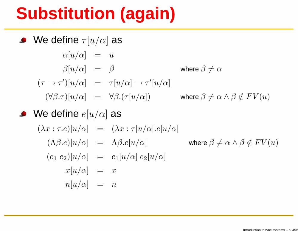
Substitution (again)We define τ [u/α] as
α[u/α] = u
β[u/α] = β where β 6= α
(τ → τ ′)[u/α] = τ [u/α]→ τ ′[u/α]
(∀β.τ)[u/α] = ∀β.(τ [u/α]) where β 6= α ∧ β /∈ FV (u)
We define e[u/α] as(λx : τ.e)[u/α] = (λx : τ [u/α].e[u/α]
(Λβ.e)[u/α] = Λβ.e[u/α] where β 6= α ∧ β /∈ FV (u)
(e1 e2)[u/α] = e1[u/α] e2[u/α]
x[u/α] = x
n[u/α] = n
Introduction to type systems – p. 45/59
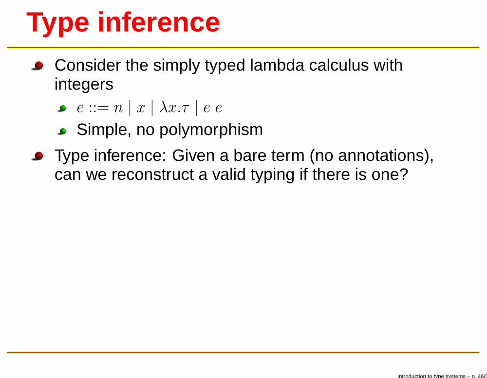
Type inferenceConsider the simply typed lambda calculus withintegers
e ::= n | x | λx.τ | e e
Simple, no polymorphism
Type inference: Given a bare term (no annotations),can we reconstruct a valid typing if there is one?
Introduction to type systems – p. 46/59
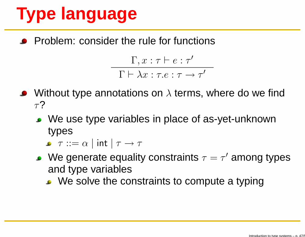
Type languageProblem: consider the rule for functions
Γ, x : τ ⊢ e : τ ′
Γ ⊢ λx : τ.e : τ → τ ′
Without type annotations on λ terms, where do we findτ?
We use type variables in place of as-yet-unknowntypesτ ::= α | int | τ → τ
We generate equality constraints τ = τ ′ among typesand type variables
We solve the constraints to compute a typing
Introduction to type systems – p. 47/59
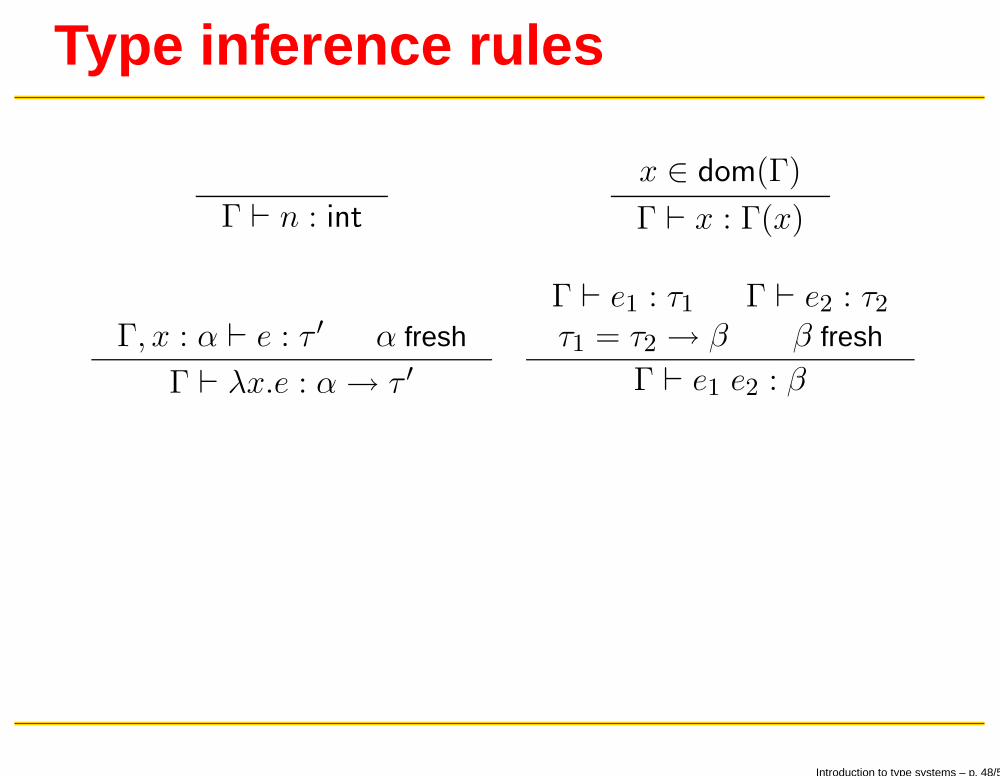
Type inference rules
Γ ⊢ n : int
x ∈ dom(Γ)
Γ ⊢ x : Γ(x)
Γ, x : α ⊢ e : τ ′ α fresh
Γ ⊢ λx.e : α→ τ ′
Γ ⊢ e1 : τ1 Γ ⊢ e2 : τ2τ1 = τ2 → β β fresh
Γ ⊢ e1 e2 : β
Introduction to type systems – p. 48/59
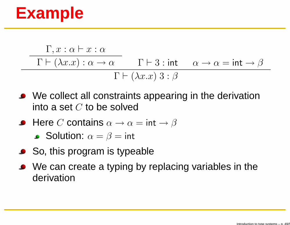
Example
Γ, x : α ⊢ x : α
Γ ⊢ (λx.x) : α→ α Γ ⊢ 3 : int α→ α = int→ β
Γ ⊢ (λx.x) 3 : β
We collect all constraints appearing in the derivationinto a set C to be solved
Here C contains α→ α = int→ β
Solution: α = β = int
So, this program is typeable
We can create a typing by replacing variables in thederivation
Introduction to type systems – p. 49/59
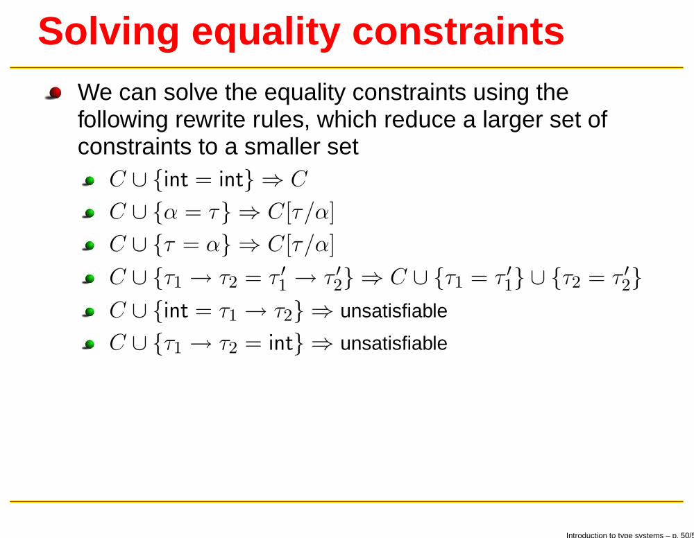
Solving equality constraintsWe can solve the equality constraints using thefollowing rewrite rules, which reduce a larger set ofconstraints to a smaller set
C ∪ {int = int} ⇒ C
C ∪ {α = τ} ⇒ C[τ/α]
C ∪ {τ = α} ⇒ C[τ/α]
C ∪ {τ1 → τ2 = τ ′1 → τ ′2} ⇒ C ∪ {τ1 = τ ′1} ∪ {τ2 = τ ′2}
C ∪ {int = τ1 → τ2} ⇒ unsatisfiable
C ∪ {τ1 → τ2 = int} ⇒ unsatisfiable
Introduction to type systems – p. 50/59
TerminationWe can prove that the constraint solving algorithmterminates
For each rewriting rule, eitherWe reduce the size of the constraint setWe reduce the number of “arrow” constructors in theconstraint set
As a result, the constraint always gets “smaller” andeventually becomes empty
A similar argument is made for strong normalizationof the simply-typed lambda calculus
Introduction to type systems – p. 51/59

Occurs checkWe don’t have recursive types, so we don’t infer them
In the operation C[τ/α] we require that α /∈ FV (τ)
In practice, it may be better to allow α ∈ FV (τ) andperform an occurs check at the end
Could be difficult to implementUnification might not terminate without occurs check
Introduction to type systems – p. 52/59
Unifying a variable and a typeComputing C[τ/α] by substitution is inefficient
Instead, use a union-find data structure to representequal types
The terms are in a union-find forestWhen a variable and a term are equated, we unionthem so they have the same equivalence classIf there is a concrete type in an equivalence class,use it to represent the classSolution is the representative of each class at theend
Introduction to type systems – p. 53/59
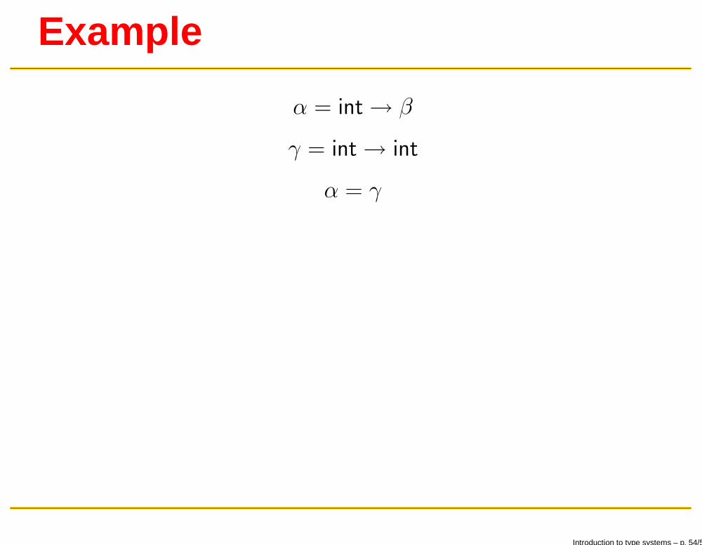
Example
α = int→ β
γ = int→ int
α = γ
Introduction to type systems – p. 54/59
UnificationThe process of finding a solution to a set of equalityconstraints is called unification
Original algorithm by Robinson (inefficient)Often written in different form (algorithm W)Usually solved on-line as type rules are applied
Introduction to type systems – p. 55/59
DiscussionThe algorithm we’ve given finds the most general typeof a term
Any other type is “more specific”Formally, any other valid type can be created fromthe most general type by applying a substitution ontype variables
All this is for a monomorphic type system, noquantification
Variables α stand for “some particular type”
Introduction to type systems – p. 56/59
Inference for polymorphismWe would like to have the power of System F, and theease of use of type inference
In short: given an untyped lambda calculus term,can we discover the annotations necessary for typingthe term in System F, if such a typing is possible?Unfortunately, no. This problem has been shown tobe undecidable.
Can we at least perform some kind of parametricpolymorphism
Yes, a “sweet spot” was found by Hindley and MilnerAbstraction at let-statements, instantiation on eachvariable useUsed in ML
Introduction to type systems – p. 57/59
Curry-Howard extensionDoes the equivalent logic get extended usingpolymorphism?
More than enough to encode first-order logicA subset of System F (with several restrictions) isequivalent to First Order Logic
Actually, we can use System F as a common languagefor polymorphic lambda calculus and for second-orderpropositional logic!
Introduction to type systems – p. 58/59
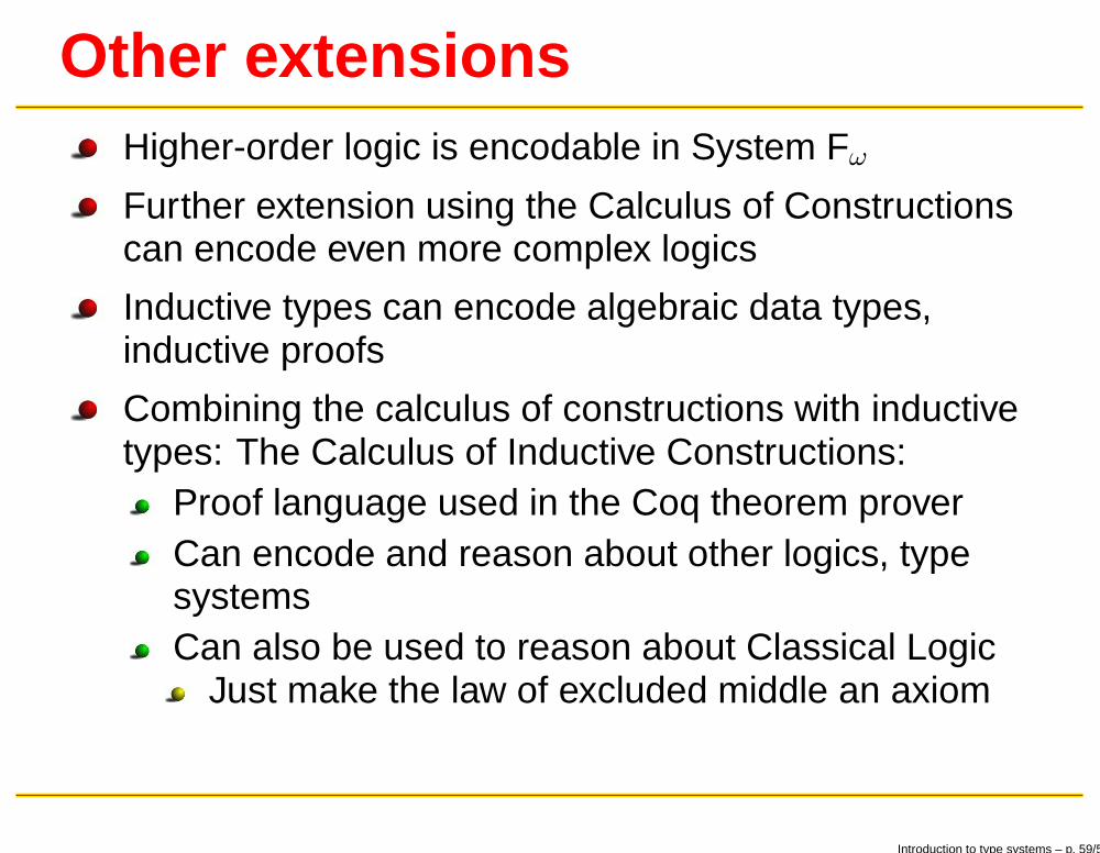
Other extensionsHigher-order logic is encodable in System Fω
Further extension using the Calculus of Constructionscan encode even more complex logics
Inductive types can encode algebraic data types,inductive proofs
Combining the calculus of constructions with inductivetypes: The Calculus of Inductive Constructions:
Proof language used in the Coq theorem proverCan encode and reason about other logics, typesystemsCan also be used to reason about Classical Logic
Just make the law of excluded middle an axiom
Introduction to type systems – p. 59/59

![Queries on TreesAutomata, logic, and XML [Nev02b, Nev02a] Automata for XML – a survey [Sch07] Effective Characterizations of Tree Logics [Boj08a] Treewalking automata [Boj08b] Books](https://static.fdocument.org/doc/165x107/5fde4ddcef0206202f21ac29/queries-on-trees-automata-logic-and-xml-nev02b-nev02a-automata-for-xml-a.jpg)