
IntroductiontoPhotonics ——— Draft · IntroductiontoPhotonics ——— Draft ... Preface...
208
Introduction to Photonics ——— Draft Technical University of Clausthal WS 2000/2001 – WS 2004/2005 W. L¨ ucke
Transcript of IntroductiontoPhotonics ——— Draft · IntroductiontoPhotonics ——— Draft ... Preface...
Introduction to Photonics
———
Draft
Technical University of ClausthalWS 2000/2001 – WS 2004/2005
W. Lucke

3
Preface
Photonics deals with controlled production, evolution, and detection of (mainlycoherent) light (photons) within the ‘optical’ region of the electromagnetic spectrum(vacuum wavelength (λ0) from 50 nm to 500 µm or photon energies (~ω) from 25 to0.002 eV). With the advent of the laser non-linear properties of optical media havebecome essential.
...
This draft should be considered as just the germ of a more complete introductionto photonics.
Recommended Literature: (Loudon, 2000; Mandel and Wolf, 1995;Yariv, 1997; Vogel et al., 2001; Shen, 1984; Bachor, 1998; Saleh and Teich, 1991)

4
Contents
1 Fundamentals 91.1 Classical Electrodynamics . . . . . . . . . . . . . . . . . . . . . . . . 9
1.1.1 Maxwell Equations . . . . . . . . . . . . . . . . . . . . . . . 91.1.2 Energy and Energy Flux of the Field . . . . . . . . . . . . . . 111.1.3 Frequency Analysis . . . . . . . . . . . . . . . . . . . . . . . . 12
1.2 Quantized Electromagnetic Radiation . . . . . . . . . . . . . . . . . . 131.2.1 Quantum Aspects of Light . . . . . . . . . . . . . . . . . . . . 141.2.2 Field Operators . . . . . . . . . . . . . . . . . . . . . . . . . . 141.2.3 Field Modes . . . . . . . . . . . . . . . . . . . . . . . . . . . . 191.2.4 ‘Classical’ States of Light . . . . . . . . . . . . . . . . . . . . 24
2 Linear Optical Media 352.1 General Considerations . . . . . . . . . . . . . . . . . . . . . . . . . . 35
2.1.1 A Simple Model . . . . . . . . . . . . . . . . . . . . . . . . . . 352.1.2 Exploiting Homogeneity . . . . . . . . . . . . . . . . . . . . . 372.1.3 Radiation off a Given Source . . . . . . . . . . . . . . . . . . . 40
2.2 Monochromatic Waves of Exponential Type . . . . . . . . . . . . . . 422.2.1 Basic Equations . . . . . . . . . . . . . . . . . . . . . . . . . . 422.2.2 Simple Reflection and Refraction . . . . . . . . . . . . . . . . 442.2.3 Birefringent Media (Crystal Optics) . . . . . . . . . . . . . . . 51
2.3 Monochromatic Light Rays . . . . . . . . . . . . . . . . . . . . . . . . 572.4 Group-Velocity Dispersion . . . . . . . . . . . . . . . . . . . . . . . . 59
3 Nonlinear Optical Media 613.1 General Considerations . . . . . . . . . . . . . . . . . . . . . . . . . . 61
3.1.1 Functionals of the Electric Field . . . . . . . . . . . . . . . . . 623.1.2 Various Electric Polarization Effect . . . . . . . . . . . . . . . 633.1.3 Perturbative Solution of Maxwell’s Equations . . . . . . . . 63
3.2 Classical Nonlinear Optical Effects . . . . . . . . . . . . . . . . . . . 653.2.1 Phase Matching . . . . . . . . . . . . . . . . . . . . . . . . . . 653.2.2 Three-Wave Mixing . . . . . . . . . . . . . . . . . . . . . . . . 703.2.3 Four-Wave Mixing . . . . . . . . . . . . . . . . . . . . . . . . 76
3.3 Quantum Aspects of Three-Wave Mixing . . . . . . . . . . . . . . . . 773.3.1 Quantized Radiation Inside Linear Media . . . . . . . . . . . . 77
5
6 CONTENTS
3.3.2 Nonlinear Perturbation . . . . . . . . . . . . . . . . . . . . . . 793.3.3 Type-II Spontaneous Down Conversion . . . . . . . . . . . . . 81
4 Photodetection 834.1 Simple Detector Models . . . . . . . . . . . . . . . . . . . . . . . . . 83
4.1.1 Single Localized Detectors . . . . . . . . . . . . . . . . . . . . 834.1.2 Independent Detectors . . . . . . . . . . . . . . . . . . . . . . 85
4.2 Quantum Theory of Coherence . . . . . . . . . . . . . . . . . . . . . 864.2.1 Correlation Functions in General . . . . . . . . . . . . . . . . 864.2.2 Correlation Functions of Single-Mode States . . . . . . . . . . 88
4.3 Simple Interference Experiments . . . . . . . . . . . . . . . . . . . . . 954.3.1 Young’s Double-Slit Experiment . . . . . . . . . . . . . . . . 954.3.2 Hanbury-Brown-Twiss Effect . . . . . . . . . . . . . . . . 95
5 Applications of Non-Classical Light 995.1 Criteria for Non-Classical Light . . . . . . . . . . . . . . . . . . . . . 995.2 The Action of Beam Splitters on Photons . . . . . . . . . . . . . . . . 102
5.2.1 General Action of Linear Optical Devices . . . . . . . . . . . . 1025.2.2 Classical Description of Lossless Beam Splitters . . . . . . . . 1035.2.3 Transformation of Photon Modes . . . . . . . . . . . . . . . . 1055.2.4 Mach-Zehnder Interferometer . . . . . . . . . . . . . . . . . 109
5.3 Applications to Quantum Information Processing . . . . . . . . . . . 1115.3.1 Single-Photon States and Quantum Cryptography . . . . . . . 1115.3.2 Entangled Pairs of Photons . . . . . . . . . . . . . . . . . . . 1145.3.3 Quantum Teleportation . . . . . . . . . . . . . . . . . . . . . 116
6 Coupling of Quantum Systems 1276.1 Closed Systems . . . . . . . . . . . . . . . . . . . . . . . . . . . . . . 127
6.1.1 States and Observables in the Heisenberg Picture . . . . . . . 1276.1.2 Time Evolution and Projective Measurements . . . . . . . . . 1306.1.3 Time Dependent Perturbation Theory . . . . . . . . . . . . . 132
6.2 Bipartite Systems . . . . . . . . . . . . . . . . . . . . . . . . . . . . . 1336.2.1 Composition of Distinguishable Systems . . . . . . . . . . . . 1336.2.2 Partial States . . . . . . . . . . . . . . . . . . . . . . . . . . . 1346.2.3 Composition of Indistinguishable Systems . . . . . . . . . . . 135
6.3 Open Systems . . . . . . . . . . . . . . . . . . . . . . . . . . . . . . . 137
7 Radiative Transitions 1397.1 Single Atoms in General . . . . . . . . . . . . . . . . . . . . . . . . . 139
7.1.1 Naive Interaction Picture . . . . . . . . . . . . . . . . . . . . . 1397.1.2 Electric Field Representation . . . . . . . . . . . . . . . . . . 1427.1.3 First Order Perturbation Theory . . . . . . . . . . . . . . . . 144
7.2 Photoelectric Detection of Light . . . . . . . . . . . . . . . . . . . . . 1477.2.1 Ionisation of One-Electron Atoms . . . . . . . . . . . . . . . . 1477.2.2 Simple Photodetectors . . . . . . . . . . . . . . . . . . . . . . 150
CONTENTS 7
8 Few-Level Atomic Systems 1538.1 The Exterior Electric Field Representation . . . . . . . . . . . . . . . 1538.2 2-Level Systems . . . . . . . . . . . . . . . . . . . . . . . . . . . . . . 154
8.2.1 Interpretation of the Bloch Vector . . . . . . . . . . . . . . . 1578.2.2 Rotating Wave Approximation . . . . . . . . . . . . . . . . . . 158
8.3 3-Level Atoms . . . . . . . . . . . . . . . . . . . . . . . . . . . . . . . 1618.3.1 Population Trapping . . . . . . . . . . . . . . . . . . . . . . . 1618.3.2 Electromagnetically Induced Transparency . . . . . . . . . . . 1638.3.3 Change of Linear Susceptibility . . . . . . . . . . . . . . . . . 165
9 Cavity QED 1739.1 The Jaynes-Cummings Model . . . . . . . . . . . . . . . . . . . . . 173
9.1.1 Quantized Radiation Field for Selected Modes . . . . . . . . . 1739.1.2 Interaction of the Two-Level System with the Cavity Field . . 174
A Appendix 181A.1 Functional Taylor Expansion . . . . . . . . . . . . . . . . . . . . . . . 181A.2 Elementary Quantum Mechanics . . . . . . . . . . . . . . . . . . . . . 183
A.2.1 Scalar Particles in One Dimension . . . . . . . . . . . . . . . . 183A.2.2 Energy Eigenstates of the Harmonic Oscillator . . . . . . . . . 185A.2.3 Coherent States . . . . . . . . . . . . . . . . . . . . . . . . . . 188
A.3 Construction of Field Operators . . . . . . . . . . . . . . . . . . . . . 189A.4 Dyson Series . . . . . . . . . . . . . . . . . . . . . . . . . . . . . . . 191
Bibliography 193
Index 206

8 CONTENTS

Chapter 1
Fundamentals
1.1 Classical Electrodynamics
1.1.1 Maxwell Equations
The classical electromagnetic field E(x, t) , B(x, t) is defined (implicitly) by theforce density
f(x, t) = ρtest(x, t)E(x, t) + test(x, t)×B(x, t) (1.1)
that it exerts on the carriers of test 4-current densities(c ρtest(x, t), test(x, t)
); see,
e.g., Sections 3.3.3 and 4.1.3 of (Lucke, rel). The field generated by a 4-current
density(c ρ(x, t), (x, t)
)fulfilling the continuity equation
ρ(x, t) + div (x, t) = 0 (1.2)
has to obey Maxwell’s equations1
curlB(x, t) = µ0
(ǫ0∂
∂tE(x, t) + (x, t)
), (1.3)
curlE(x, t) = − ∂
∂tB(x, t) ,
divE(x, t) =1
ǫ0ρ(x, t) ,
divB(x, t) = 0
(we use SI units; see Appendix A.3.3 of (Lucke, edyn)). More precisely, in theclassical case, it is the physical solution
E(x, t) = −gradΦret(x, t)−∂
∂tAret(x, t) , B(x, t) = curlAret(x, t)
Draft, November 5, 2011
1Note that µ0 ǫ0 = c−2 , where
ǫ0 ≈ 8, 85 · 10−12 As
Nm
and c denotes the velocity of light in vacuum (≈ 3 · 108 m/s).
9
10 CHAPTER 1. FUNDAMENTALS
given by the retarded electromagnetic Potentials
Φret(x, t) =1
ǫ0
∫ ρ(x′, t− |x−x′|
c
)
4π |x− x′| dVx′ ,
Aret(x, t) = µ0
∫ (x′, t− |x−x′|
c
)
4π |x− x′| dVx′ .
(1.4)
In typical applications the 4-current density is approximated as
ρ(x, t) = ρex(x, t)− divP(x, t) ,
(x, t) = ex(x, t) +∂
∂tP(x, t) ,
(1.5)
with some known 4-current density(c ρex(x, t), ex(x, t)
)of excess charges and some
generalized polarization P(x, t) .
Remarks:
1. For every choice of ρex(x, t), ex(x, t) obeying the continuity equation there is2
a time-dependent vector field P(x, t) fulfilling (1.5).
2. Under suitable conditions we have
∂
∂tP(x, t) =
∂
∂tPel(x, t) +
1
µ0rotM(x, t) , (1.6)
(see, e.g., Chapter 4 of (Lucke, edyn)), where Pel(x, t) = D(x, t) − ǫ0 E(x, t)denotes the electric dipole density and M(x, t) = B(x, t) − µ0 H(x, t) themagnetic dipole density.3
Then Maxwell’s equation become equivalent to
curlB(x, t) = µ0∂
∂t
(ǫ0 E(x, t) +P(x, t)
)+ µ0 ex(x, t) , (1.7)
curlE(x, t) = − ∂
∂tB(x, t) , (1.8)
div(ǫ0 E(x, t) +P(x, t)
)= +ρex(x, t) , (1.9)
divB(x, t) = 0 . (1.10)
Draft, November 5, 2011
2See (Lucke, 1995), in this connection.3Contrary to a wrong argument given in (Landau und Lifschitz, 1967, § 60) the interpretation
of M(x, t) does not imply ∂∂t Pel(x, t) ≈ 0 for ex(x, t) = 0 . For higher dipole moments see
(Bloembergen, 1996b, p. 63).
1.1. CLASSICAL ELECTRODYNAMICS 11
1.1.2 Energy and Energy Flux of the Field
For arbitrary (sufficiently well-behaved) regions G we have
∫
Gµ0 (x, t) · E(x, t) dVx
=(1.3)
∫
G
(E(x, t) ·
(∇x ×B(x, t)
)
︸ ︷︷ ︸=B(x,t)·(∇x ×E(x, t)︸ ︷︷ ︸
=
(1.8)
− ∂∂t
B(r,t)
)−∇x·(E(x,t)×B(x,t))
−ǫ0 µ0 E(x, t) ·∂
∂tE(x, t)
)dVx
= −∫
G
(ǫ0 µ0E(x, t) ·
∂
∂tE(x, t) +B(x, t) · ∂
∂tB(x, t) +∇x ·
(E(x, t)×B(x, t)
))dVx .
This implies1
2
∂
∂t
(ǫ0 |E(x, t)|2 + 1
µ0
|B(x, t)|2)
= −(x, t) · E(x, t)−∇x ·E(x, t)×B(x, t)
µ0
(1.11)
and therefore, by Gauß’ theorem, the Poynting theorem 4
d
dt
∫
G
1
2
(ǫ0 |E(x, t)|2 + 1
µ0
|B(x, t)|2)dVx
= −∫
G(x, t) · E(x, t) dVx −
∫
∂G
E(x, t)×B(x, t)
µ0
· dSx .
(1.12)
Remark: If (1.6) holds then (1.12) and Gauß’s theorem, because of
div(E(x, t)×M(x, t)
)= M(x, t) · curlE(x, t)−E(x, t) · curlM(x, t)
(1.8) −M(x, t) · ∂∂t
B(x, t)−E(x, t) · curlM(x, t) ,
also imply
∫
G
(E(x, t) · ∂
∂tD(x, t) +H(x, t)
∂
∂tB(x, t)
)dVx
= −∫
G
ex(x, t) ·E(x, t) dVx −∫
∂G
(E(x, t)×H(x, t)
)· dSx ,
(1.13)
where
D(x, t)def= ǫ0 E(x, t) +P(x, t) , H(x, t)
def=
B(x, t)−M(x, t)
µ0.
Draft, November 5, 2011
4See also (Kinsler et al., 2009).
12 CHAPTER 1. FUNDAMENTALS
Since, by (1.1),
∫
G(x, t) · E(x, t) dVx is to be interpreted as the rate of the work
done by the electromagnetic field on the charges, (1.12) suggests the interpretation
S(x, t)def=
1
µ0
E(x, t)×B(x, t) =
engergy current density of theplain electromagnetic field
(1.14)
of the (free) Poynting vector S(x, t) and
H0(x, t)def=
1
2
(ǫ0 |E(x, t)|2 + 1
µ0
|B(x, t)|2)
=
energy density of theplain electromagnetic field .
(1.15)
Assuming (1.5) and defining5
U(x, t) def=
work done by the fieldon the non-excess charges .
we get∂
∂tU(x, t) =
(1.1)E(x, t) · ∂
∂tP(x, t) . (1.16)
Remark: Recall that the power performed by a force F(t) on a masspoint withtrajectory x(t) is F(t) · x(t) . Correspondingly, the power performed by the angularmomentum M(t) on a rigid body rotating with circular angular velocity ω(t) isM · ω(t) . Likewise, the power performed by an electrical field E(t) on an electrical
dipole P(t) is E(t) · P(t) — notd
dt(E(t) ·P(t)) .
Therefore, (1.11) and (1.5) imply
∂
∂t
(H0(x, t) + U(x, t)
)= −ex(x, t) · E(x, t)−∇x ·
E(x, t)×B(x, t)
µ0
.
Consequently:
ex = 0 =⇒ d
dt
∫ (H0(x, t) + U(x, t)
)dVx = 0 . (1.17)
1.1.3 Frequency Analysis
Using the Fourier transform
f(x, ω)def=
1√2π
∫f(x, t) eiω t dt
Draft, November 5, 2011
5Concerning the classical field energy see (Landau und Lifschitz, 1967, Chapt. IX, § 61).
1.2. QUANTIZED ELECTROMAGNETIC RADIATION 13
resp.
f (x, ω)def=
1√2π
∫f(x, t) eiω t dt
we may write (1.7)–(1.10) in the equivalent form
1
µ0
curl B(x, ω) = −i ω(ǫ0 E(x, ω) + P(x, ω)
)+ ex(x, ω) , (1.18)
curl E(x, ω) = +i ω B(x, ω) , (1.19)
div(ǫ0 E(x, ω) + P(x, ω)
)= +ρex(x, ω) , (1.20)
div B(x, ω) = 0 . (1.21)
Remark: If the Fourier-integrals do not exist in the ordinary sense — as, e.g., formonochromatic waves — they have to be interpreted in the distributional sense; seeExercise 33 of (Lucke, qft) or Section 3.1.1 of (Lucke, ftm).
The continuity equation for ρex, ex implies
ρex(x, ω) =1
iωdiv ex(x, ω) ∀ω 6= 0 (1.22)
and, consequently, equivalence of the equations (1.18)–(1.21) to
B(x, ω) =1
i ωcurl E(x, ω) ∀ω 6= 0
and
curl(curl E(x, ω)
)=(ωc
)2 (E(x, ω) +
1
ǫ0P(x, ω)
)+ i ω µ0 ex(x, ω) (1.23)
for ω 6= 0 .
Of course, the physical fields have to be real. For the electric field, e.g., thismeans
E(x, t) =(E(x, t)
)∗,
i.e.E(x,−ω) =
(E(x, ω)
)∗. (1.24)
Therefore, it is sufficient to determine E(x, ω) for ω ≥ 0 .
1.2 Quantized Electromagnetic Radiation
Of course, the classical electromagnetic theory should be quantized.6 A rigorousrelativistic quantum theory describing the interaction of radiation with matter (non-perturbative QED) does not yet exist. Fortunately, as we will see, for many importantapplications the classical macroscopic Maxwell theory supplies sufficient informa-tion concerning the influence of linear optical devices on photons.7
Draft, November 5, 2011
6For a detailed discussion why a semiclassical theory (treating only ‘particles’ quantum me-chanically) plus vacuum fluctuations is insufficient see, e.g., (Scully and Zubairy, 1999).
7The notion ‘photon’ was introduced in (Lewis, 1926). See (Lamb, Jr., 1995) for a historicalreview.
14 CHAPTER 1. FUNDAMENTALS
1.2.1 Quantum Aspects of Light
Nowadays (almost) monochromatic electromagnetic radiation of angular frequencyω is considered to be composed of quanta (photons) having (total) energy ~ω each(and zero rest mass). This leads to additional information on optical processes.
To give an example, consider second harmonic generation which has to be con-sidered as formation of quanta having energy 2 ~ω out of pairs of quanta having en-ergy ~ω each.8 Reversibility of quantum dynamics predicts also the reverse process,called spontaneous down conversion: instantaneous formation of pairs of photonsout of single photons. Contrary to the quantized theory9 classical optics does notgive any hint at (essentially) simultaneous creation of both partners of each pair, asconfirmed by experiment.10
More generally, quantum optics describes multi-photon processes mediated bymatter. These processes are called nonlinear if what happens to a photon dependsin an essential way on the presence and properties of other optical photons.11 Thiskind of nonlinearity is essential for optical implementations of modern quantuminformation processing.
1.2.2 Field Operators
In the so-called radiation gauge a classical electromagnetic vacuum field E(x, t) ,B(x, t) (of sufficiently rapid decrease at spatial infinity) may be represented in theform
B(x, t) = curlA(x, t) , E(x, t) = − ∂
∂tA(x, t) (1.25)
with the vector potential
A(x, t) =1
4π
∫curlB(x′, t)
|x− x′| dVx′ (1.26)
fulfilling the Coulomb condition
divA(x, t) = 0 , (1.27)
Remark: Equations (1.25) follow from (1.26) by curl curl = grad div −∆ and the
Poisson equation ∆x
1
|x− x′| = −4π δ (x− x′) ; see, e.g., equations 4.87 and 4.63 of
(Lucke, ein). The Coulomb condition follows for (1.26) by div curl = 0 ; see, e.g.,Equation 4.89 of (Lucke, ein).
Draft, November 5, 2011
8Momentum conservation holds for the momenta inside the medium, corresponding to phase(-velocity) matching from the classical point of view.
9See (Mandel and Wolf, 1995, Sect. 22.4.2).10See (Mandel and Wolf, 1995, Sect. 22.4.7).11This type of nonlinearity does not contradict the fundamental linearity of quantum mechanical
time evolution!
1.2. QUANTIZED ELECTROMAGNETIC RADIATION 15
In this gauge the free Maxwell equations are equivalent to the vectorial waveequation
A(x, t) = 0 , def= ∆−
(1
c
∂
∂t
)2
. (1.28)
If no boundary conditions are imposed, every (sufficiently well-behaved, real) solu-tion of (1.28) fulfilling the Coulomb condition is of the form
A(x, t)def= A(+)(x, t) +
(A(+)(x, t)
)∗(1.29)
with a complex vector potential 12
A(+)(x, t) = (2π)−3/2√µ0~c
∫ ( 2∑
j=1
ǫj(k) aj(k)
)e−i(c|k|t−k·x) dVk√
2 |k|, (1.30)
where the aj(k) are (sufficiently well-behaved) complex-valued functions and theǫj(k) are vector-valued functions forming a
right handed orthonormal basis
ǫ1(k), ǫ2(k),
k
|k|
of R3
for every k 6= 0 .In the Heisenberg picture the observables E(x, t) and B(x, t) should obey the
same linear relations as their classical counter parts E(x, t) and B(x, t) . This can beachieved replacing the complex-valued functions aj(k) by suitable operator-valuedfunctions aj(k) :
A(+)(x, t)def= (2π)−3/2
õ0~c
∫ ( 2∑
j=1
ǫj(k) aj(k)
)e−i(c|k|t−k·x) dVk√
2 |k|, (1.31)
B(+)(x, t)def= curl A(+)(x, t) (1.32)
= (2π)−3/2√µ0~c
2∑
j=1
∫ik× ǫj(k) aj(k) e
−i(c|k|t−k·x) dVk√2 |k|
,
E(+)(x, t)def= − ∂
∂tA(+)(x, t) (1.33)
= (2π)−3/2√µ0~c
2∑
j=1
∫ic |k| ǫj(k) aj(k) e−i(c|k|t−k·x) dVk√
2 |k|,
Draft, November 5, 2011
12The factor 1/√
2 |k| under the integral will be necessary for Lorentz covariance of the quan-tized field tensor. The factor
õ0~c is chosen in view of (1.57).
16 CHAPTER 1. FUNDAMENTALS
A(x, t)def= A(+)(x, t) +
(A(+)(x, t)
)†, (1.34)
B(x, t)def= B(+)(x, t) +
(B(+)(x, t)
)†, (1.35)
E(x, t)def= E(+)(x, t) +
(E(+)(x, t)
)†. (1.36)
If the operators aj(k) , (aj(k))† fulfill the canonical commutation relations 13
[aj(k), aj′(k′)]− = 0 ,
[aj(k),
(aj′(k
′))†]
−= δjj′ δ(k− k′) (1.37)
on a suitable dense subspace D0 , of the Hilbert space Hfield , containing a cyclicnormalized vacuum state vector Ω characterized by14
aj(k) Ω = 0 , (1.38)
then the observables B(+)(x, t) , E(+)(x, t) fulfill all reasonable physical postulates.
Remarks:
1. These properties fix the quantized theory up to unitary equivalence (see Sect.4.1.1 of (Lucke, qft) and (Fredenhagen, 2001, Sect. III.4)). This also implies, bythe way, that all irreducible realizations of (1.37)/(1.38) are unitarily equivalent.
2. Actually, the (aj(k))†have to be considered as operator-valued distributions
(generalized functions):
∫a†j(k)ϕ
∗(k) dk ⊂(∫
aj(k)ϕ(k) dk
)†
∀ϕ ∈ S(R3) .
See, e.g., Section 2.1.3 of (Lucke, qft) for details.
Especially, the field observables fulfill the quantized free Maxwell equations:
curl B(x, t) = µ0 ǫ0∂
∂tE(x, t) , (1.39)
curl E(x, t) = − ∂
∂tB(x, t) , (1.40)
div E(x, t) = 0 , (1.41)
div B(x, t) = 0 . (1.42)
Draft, November 5, 2011
13We simply write z for z 1 , z ∈ C , as long as this does not cause any confusion. For a possiblerealization of (1.37)/(1.38) see A.3.
14Because of (1.38) the aj(k) are called annihilation operators (see(Mizrahi and Dodonov, 2002) in this connection). Here, ‘cyclic’ means that the linear spanof all vectors of the form
∫f(k1, . . . ,kn)
(aj1(k1)
)† · · ·(ajn(k1)
)†dVk1
. . . dVkn
︸ ︷︷ ︸def= 1 forn=0
Ω , n ∈ Z+ , j1, . . . , jn ∈ 1, 2 ,
with square integrable f ’s is dense in Hfield .
1.2. QUANTIZED ELECTROMAGNETIC RADIATION 17
However, the canonical commutation relations also imply[(Aj1)(+)(x1, t1) ,
((Aj2)(+)(x2, t2)
)†]
−
= i µ0 ~ c
δj1j2 −
∂
∂xj11
∂
∂xj21
∆x1
∆
(+)0 (x1 − x2, t1 − t2)
(1.43)
(in the distributional sense), where
∆(+)0 (x, t)
def= −i (2π)−3
∫eik·x e−i c|k|t
dVk2 |k| (1.44)
= −i (2π)−3∫
k0>0
δ(k0 k0 − k · k
)e−i(k
0ct−k·x) dVk dk0 .
Outline of proof for (1.43): Since
2∑
j=1
ǫj1j (k) aj(k) ,
2∑
j′=1
ǫj2j′ (k
′)(aj′(k
′))†−
=
2∑
j,j′=1
ǫj1j (k) ǫj2j′ (k′)
[aj(k) ,
(aj′(k
′))†]
−
=
2∑
j=1
ǫj1j (k) ǫj2j (k′) δ (k− k′) ,
(1.31) implies[(Aj1)(+)(x1, t1) ,
((Aj2)(+)(x2, t2)
)†]
−
= (2π)−3µo ~ c
∫ 2∑
j=1
ǫj1j (k) ǫj2j (k′)
︸ ︷︷ ︸=δj1j2
− kj1kj2
|k|2
e−i(c|k|(t1−t2)−k·(x1−x2))dVk2 |k| .
(1.43) implies
[Aj1(x1, t1) , A
j2(x2, t2)]−
= i µ0 ~ c
(δj1j2 −
∂
∂xj11
∂
∂xj21
∆x1
)∆0(x1 − x2, t1 − t2) ,
(1.45)
where15
∆0(x, t)def= ∆
(+)0 (x, t)−∆
(+)0 (−x,−t) . (1.46)
Draft, November 5, 2011
15Note that ∆0(x, t) , being an anti-symmetric Lorentz invariant distribution, vanishes forc |t| ≥ |x| . However, the operator on the r.h.s of (1.45) is non-local.
18 CHAPTER 1. FUNDAMENTALS
Therefore, we have ⟨Ω∣∣∣ E(x, t) · E(x′, t′) Ω
⟩6= 0 (1.47)
in spite of 16 ⟨Ω∣∣∣ E(x, t) Ω
⟩= 0 .
Since E(x, t) is the observable of the electric field,17 field, (1.47) shows the presenceof vacuum fluctuations18 (quantum noise). (1.45) also implies19
[Aj1(x1, t) , A
j2(x2, t)]−
= 0 ,
[Aj1(x1, t) , B
j2(x2, t)]−
= 0 (1.48)
[Bj1(x1, t) , B
j2(x2, t)]−
= 0 ,
[Ej1(x1, t) , E
j2(x2, t)]−
= 0
and[Aj1(x1, t) , E
j2(x2, t)]−
= −i ~ǫ0δj1j2⊥ (x1 − x2) , (1.49)
[B(x1, t) , E
j2(x2, t)]−
= i~
ǫ0ej2 ×∇x1δ(x1 − x2) ,
where
δj1j2⊥ (x)def= (2π)−3
∫ (δj1j2 −
kj1kj2
|k|2)eik·x dVk (1.50)
fulfills3∑
j,j′=1
∫δjj
′
⊥ (x− x′)F j(x′) dVx′ ej′ = F⊥(x)
def= F(x) + grad
∫divF(x′)
4π |x− x′| dVx′ (1.51)
for sufficiently well-behaved F(x) .
Draft, November 5, 2011
16Also for Johnson noise, the electric current in a simple circuit resulting from fluctuatingelectromagnetic forces due to thermal motion of the charges, one has zero mean but nonzero meansquare. Ω being an eigenvector of the (non-hermitean!) operator E(+)(x, t) does not mean thatthe positive-frequency part of the electric field has a definite value in the vacuum state.
17I.e.⟨Φ∣∣∣ E(x, t) Φ
⟩is the expectation value for the electric field in the quantum state Φ , for
all Φ ∈ D0 .18These provide, e.g., a simple explanation for the spontaneous transitions of exited atoms
into lower energy states; see (Milonni, 1994, Chapter 3) for some further effects. Also spontaneousdown-conversion can be explained as a result of vacuum fluctuations.
19The first three equations hold because of ∆0(x, 0) = 0 . The last one follows from(∂
∂t
)2
∆0(x, t)|t=0= 0 .
1.2. QUANTIZED ELECTROMAGNETIC RADIATION 19
Remark: Note that F⊥(x) is just the transversal part of
F(x) = curl
∫curlF(x′)
4π |x− x′| dVx − grad
∫divF(x′)
4π |x− x′| dVx
(see, e.g., Section 4.5.3 of (Lucke, ein)).
Let us finally note that one may prove relativistic covariance of the theory in thesense that there is a unitary representation20 U(a,Λ) of the restricted Poincare
group P↑+ fulfilling
U(a,Λ)Ω = 0
and
U−1(a,Λ)F µν (Λx+ a) U(a,Λ) =3∑
α,β=0
ΛµαΛνβF
αβ(x)
(see, e.g., Chapter 4 of (Lucke, qft) for details), where21
(F µν(x)
)def=
0 −1cE1(x, t) −1
cE2(x, t) −1
cE3(x, t)
+ 1cE1(x, t) 0 −B3(x, t) +B2(x, t)
+ 1cE2(x, t) +B3(x, t) 0 −B1(x, t)
+ 1cE3(x, t) −B2(x, t) +B1(x, t) 0
andx
def= (x0, . . . , x3) , x0
def= c t .
This together with the above commutation relations also shows that the field mea-surements at space-like separated space-time points are compatible:
[F µν(x), F µ′ν′(x′)
]−= 0 for c |t− t′| > |x− x′| (Einstein causality) .
1.2.3 Field Modes
The free Hamiltonian Hfield , characterized as the self-adjoint operator fulfilling thecommutation relation
i
~
[Hfield, A
(+)(x, t)]−=
∂
∂tA(+)(x, t) (1.52)
Draft, November 5, 2011
20This means that the U(a,Λ) are unitary operators fulfilling
U(a1,Λ1)U(a2,Λ2) = U(a1 + Λ1a2,Λ1Λ2) ∀ (a1,Λ1), (a2Λ2) ∈ P↑+ .
21Note that Fµν is the quantized version of1
µ0Hµν , as introduced in 1.1.1.
20 CHAPTER 1. FUNDAMENTALS
on D0 ⊂ DHfieldand
HfieldΩ = 0 ,
is given by22
Hfield =
∫~ c |k| n(k) dVk , n(k)
def=
2∑
j=1
(aj(k))† aj(k) , (1.53)
where n(k) is interpreted as the observable (in the Heisenberg picture) for thek-space density of the number of photons :
∫
O〈Φ | n(k) Φ〉 dVk =
expectation value for thenumber of photons in the state Φwith momentum p = ~k ∈ ~O .
(1.54)
This is consistent in the sense that, for every open subset O of the k-space, the
t-independent observable
∫
On(k) dVk commutes23 with Hfield , has only nonnegative
integer eigenvalues,24 and
P0def=
∫~k n(k) dVk (1.55)
is the momentum observable25 as uniquely characterized (on D0) by
i
~
[P0, A
j(x, t)]−= −∇xA
j(x, t) (1.56)
andP0Ω = 0
According to (1.54),
Ndef=
∫n(k) dVk
has to be interpreted as the observable for the total number of photons and thesubspace H(n)
field of n-photon state vectors coincides with the closed linear span of the
Draft, November 5, 2011
22Note that (1.37) implies[n(k′), aj(k)
]−
= −aj(k) δ(k − k′) . This, actually, is the heuristic
motivation for (1.37). See (Green, 1953), in this connection.23Note that (1.37) implies
[(aj(k)
)†aj(k) ,
(aj′(k
′))†aj′(k
′)]−= 0 .
24Since (1.37) implies
((aj(k)
)†aj(k)
) (aj1(k1)
)† · · ·(ajn(kn)
)†
=(aj1(k1)
)† · · ·(ajn(kn)
)†(((
aj(k))†aj(k)
)+
n∑
ν=1
δjjν δ(k− kν)
),
(recall the derivation of (A.26)).25This observable is t-independent in the Heisenberg picture, since it commutes with Hfield .
1.2. QUANTIZED ELECTROMAGNETIC RADIATION 21
set of all vectors of the form26
∫f(k1, . . . ,kn)
(aj1(k1)
)†· · ·(ajn(k1)
)†dVk1 . . . dVkn
Ω
with square integrable f ’s.As already indicated in Footnote 12, the normalization factor on the r.h.s. of
(1.31) has been chosen to yield27
Hfield =1
2
∫ (ǫ0 : E(x, t) · E(x, t) : +
1
µ0
:B(x, t) · B(x, t) :
)dVx ,
c2 P0 =1
µ0
∫: E(x, t)× B(x, t) : dVx ,
(1.57)
where : : means normal ordering , i.e. in all products the creation operators
a†j(k)def=(aj(k)
)†have to be placed — irrespective of the initial ordering — to the
left of the annihilation operators aj(k) .
A dense subset of H(n)field is given by the linear span of the set of all (i.g. not yet
normalized) vectors of the forma†1 · · · a†nΩ
with modes a1, . . . an , i.e. operators of the form28
aν =2∑
j=1
∫aj(k)
(f jν (k)
)∗dVk , (1.58)
[aν , a
†ν
]− = 1 . (1.59)
Here
⟨Ω | A(+)(x, t) a†ν Ω
⟩= (2π)−
32
õ0 ~ c
∫ 2∑
j=1
ǫj(k) fjν (k) e
−i(c|k|t−k·x) dVk√2 |k|
(1.60)
Draft, November 5, 2011
26Recall Footnote 14.27Recall Footnote 1. Using the commutation relations for the components of A(x, t) , E(x, t)
and B(x, t) one can verify (1.52) and (1.56) also directly for (1.57). For the connection be-tween the energy current density and the momentum density of the electromagnetic field see(Landau und Lifschitz, 1967, Footnote 1 on Page 284).
28Equation (1.59) is equivalent to
2∑
j=1
∫ ∣∣f jν (k)∣∣2 dVk = 1 .
22 CHAPTER 1. FUNDAMENTALS
can be interpreted as wave function of the single photon29 in the (pure) state = a†ν Ω .Since⟨Ω
∣∣∣∣ aj(k)2∑
j=1
a†j(k) fj(k) dVk Ω
⟩=
⟨Ω
∣∣∣∣2∑
j=1
[aj′(k′) , a†j(k)]− f
j(k) dVk Ω
⟩
= f j′(k′) ,
for every φ(1) ∈ H(1)field there is exactly one mode a with
φ(1) = a† Ω .
Motivated by ⟨a†Ω
∣∣∣ c† Ω⟩
=⟨Ω∣∣∣ a c†Ω
⟩
=⟨Ω∣∣∣ [a , c†]− Ω
⟩
= [a , c†]− ,
modes a, c are said to be orthogonal if
[a, c†]− = 0 .
A family aνν∈N of pairwise orthogonal modes is said to bemaximal , ifa†ν Ω : ν ∈ N
is a maximal orthonormal system (MONS) of H(1)field . For every maximal family
aνν∈N of pairwise orthogonal modes we have
aj(k) =∞∑
ν=1
⟨Ω∣∣∣ aj(k) a†ν Ω
⟩aν ;
since
a†j(k) Ω =∞∑
ν=1
∣∣a†ν Ω⟩⟨a†ν Ω
∣∣ a†j(k) Ω
=∞∑
ν=1
(⟨Ω | aj(k) a†ν Ω
⟩)∗a†ν Ω (1.61)
and modes a are uniquely characterized by the corresponding 1-photon state vectorsa† Ω . Therefore, the field operators aj(k) may be replaced by the countable setof ordinary operators aν and every normalized 1-photon state vector Ψ(1) may bewritten in the form
Ψ(1) =∞∑
ν=1
λν a†ν Ω ,
∞∑
ν=1
|λν |2 = 1 ,
where the complex coefficients λ are the probability amplitudes for the ‘modes’aν , i.e.:
Draft, November 5, 2011
29If∑2j=1 ǫj(k) f
jν (k) ∝ ǫ1(k) + i ǫ2(k) resp.
∑2j=1 ǫj(k) f
jν (k) ∝ ǫ1(k) − i ǫ2(k) the photon is
said to have positive resp. negative helicity.
1.2. QUANTIZED ELECTROMAGNETIC RADIATION 23
For every ν0 ∈ N
|λν0| =∣∣∣⟨a†ν Ω
∣∣∣Ψ(1)⟩∣∣∣
2
is the probability for finding a photon, randomly chosen from an ensem-ble (characterized by) Ψ(1) , in the mode a†ν if an ideal test for being injust one one the modes a1, a2, . . . is performed.30
Obviously, for ν ∈ N ,
nνdef= a†ν aν
is the observable for the number of photons in mode aν and for the observable Nfor the total number of photons we get
N =n∑
ν=1
nν .
Warning: According to the simple theory of photodetection consideredin 7.2.2 the states corresponding to elements of H(n)
field are, in fact, n-fold localized: The maximal number of photodetectors which may firesimultaneously when testing such a state is n .
Typical for nonlinear quantum optics :
b†ν ω 7−→ c†ν Ω ∀ ν 6=⇒ b†1 · · · b†nΩ 7−→ c†1 · · · c†nΩ ∀n .
Such ‘nonlinear’ behavior is needed, e.g., for optical implementations of the CNOTgate acting according to
H⊗H 7−→ H⊗H ,H⊗V 7−→ H⊗V ,V ⊗V 7−→ V ⊗H ,V ⊗H 7−→ V ⊗V .
Finally, let us derive some useful relations for modes a :
A simple consequence of the commutation relations (1.37) and (1.59) is(a†a)a = a
(a†a− 1
),(a†a)a† = a†
(a†a+ 1
)(1.62)
which, by iteration, implies(a†a)(a)n = (a)n
(a†a− n
),(a†a) (a†)n
=(a†)n (
a†a+ n)
Draft, November 5, 2011
30Typical for quantum mechanics is, that such tests are considered even if
Ψ(1) = a† Ω , a 6= aν ∀ ν ∈ N .
24 CHAPTER 1. FUNDAMENTALS
for all n ∈ N . This, in turn, implies31
(a†)nan = (a†a)
(a†a− 1
)· · ·(a†a− (n− 1)
)∀n ∈ N (1.63)
and (a†a) (a†)n
Ω = n(a†)n
Ω ∀n ∈ N . (1.64)
1.2.4 ‘Classical’ States of Light
They are important,32 not only because they are one of the quantum mechanical stateswhose properties most closely resemble those of a classical electromagnetic wave, butalso because a single-mode laser operated well above threshold generates a coherentstate excitation...
(Loudon, 2000, p. 190)
Radiation off Classical Currents
The expectation values for the (no longer free) electromagnetic field associated with a
classical 4-current(c ρ(x, t), (x, t)
)in the vacuum should fulfill the corresponding
Maxwell equations:
curl 〈B(x, t)〉 = µ0
(ǫ0∂
∂t〈E(x, t)〉+ (x, t)
), (1.65)
curl 〈E(x, t)〉 = − ∂
∂t〈B(x, t)〉 , (1.66)
div 〈E(x, t)〉 =1
ǫ0ρ(x, t) , (1.67)
div 〈B(x, t)〉 = 0 . (1.68)
In the interaction picture the expectation values (for pure states) are given by33
〈B(x, t)〉 =⟨ΨIt
∣∣∣ B(x, t)ΨIt
⟩,
〈E(x, t)〉 =
⟨ΨIt
∣∣∣∣(E(x, t)− grad
∫ρ(x′, t)
4 π ǫ0 |x− x′| dVx′
)ΨIt
⟩ (1.69)
and, therefore, the equations (1.65)–(1.68) are guaranteed by the t-dependence
i~d
dtΨIt = Hint(t)Ψ
It , (1.70)
of the normalized state vector ΨIt , where
Hint(t)def= −
∫(x, t) · A(x, t) dVx . (1.71)
Draft, November 5, 2011
31Compare with (A.31).32See also (Klauder, 2010).33Note that, in the presence of charges, E(x, t) is only the transversal part of the observable
for the field strength in the interaction picture (see also Footnote 2 of Chapter 7).
1.2. QUANTIZED ELECTROMAGNETIC RADIATION 25
Outline of proof for (1.65)–(1.68): While (1.68) resp. (1.67) follows directly from(1.69) and (1.42) resp. (1.41), (1.66) follows according to
curl 〈E(x, t)〉 =(1.69)
curl⟨ΨIt
∣∣∣ E(x, t)ΨIt
⟩
=(1.40)
⟨ΨIt
∣∣∣∣∂
∂tB(x, t)ΨI
t
⟩
=(1.70)
∂∂t
⟨ΨIt
∣∣∣ B(x, t)ΨIt
⟩−⟨ΨIt
∣∣∣∣i
~
[Hint(t), B(x, t)
]−︸ ︷︷ ︸
=(1.71),(1.48)
0
ΨIt
⟩.
(1.65), finally, follows from
1
µ0 ǫ0curl 〈B(x, t)〉 =
(1.39)
⟨ΨIt
∣∣∣∣∂
∂tE(x, t)ΨI
t
⟩
=(1.70)
∂
∂t
⟨ΨIt
∣∣∣ E(x, t)ΨIt
⟩−⟨ΨIt
∣∣∣∣i
~
[Hint(t), E(x, t)
]−ΨIt
⟩
and
− i~
[Hint(t), E(x, t)
]−
=(1.71)
− i
~
∫(x′, t) ·
[A0(x
′, t), E(x, t)]−
dVx′
=(1.49),(1.51)
1
ǫ(x) + grad
∫div (x′)
4π ǫ0 |x− x′| dVx
=cont. eq.
1
ǫ(x, t)− ∂
∂tgrad
∫ρ(x′, t)
4π ǫ0 |x− x′| dVx′ .
Ifρ(x, t) = 0(x, t) = 0
∀ t < 0 (1.72)
then the retarded solution of (1.70), characterized by
ΨIt = Ω ∀ t < 0 ,
is34
ΨIt = eλ(t) eAt , At
def= − i
~
∫ t
−∞Hint(t
′) dt′ (1.73)
(for sufficiently well-behaved ρ, ), where
λ(t)def=
1
2
∫ t
−∞
d
dt′
[At′ , At
]−dt′ ∈ C .
Remark: We assume, without proof, that this solution is unique. For the expectationvalues this is a simple consequence of Poynting’s theorem; see, e.g., Section 5.1.2of (Lucke, edyn).
Draft, November 5, 2011
34For more complicated interactions the Dyson series (see A.4) has to be evaluated.
26 CHAPTER 1. FUNDAMENTALS
That this is a solution can be shown by application of the Baker-Hausdorff
formula 35
[A, [A, B]−
]−=[B, [A, B]−
]−= 0 =⇒ eA+B = e−
12[A,B]− eA eB . (1.74)
Outline of proof for ‘ (1.73) =⇒ (1.70)’:
d
dteAt Ω
= lim∆t→+0
eAt+∆te−At − 1
∆teAt Ω
=(1.74)
lim∆t→+0
eAt+∆t−Ate− 1
2 [At+∆t,At]− − 1
∆teAt Ω
= lim∆t→+0
e
At+∆t−At − 1
∆te− 1
2 [At+∆t,At]− +
e− 1
2 [At+∆t,At]− − 1
∆t
eAt Ω
=(1.73)
(− i
~Hint − λ′(t)
)eAt Ω .
Sincei
~
∫ t
−∞Hint(t
′) dt′ = a(t)−(a(t)
)†, (1.75)
where
a(t)def=∑
j=1,2
∫ (gj(k, t)
)∗aj(k) dVk ,
and
gj(k, t)def=
i
~
õ0~c
2 |k| ǫj(k) ·∫ t
−∞
((2π)−
32
∫ (x, t′) e−ik·x dVx
)e+i c|k|t
′dt′ ,
Draft, November 5, 2011
35For operators in finite dimensional vector spaces (1.74) may be proved as follows: Since
eλAB e−λ A and eadλAB (adC Ddef= [C, D]−) fulfill the same first order differential equation and
initial condition (for λ = 0), the Campbell-Hausdorff formula
eA B e−A = eadA B
holds for arbitrary A , B . Therefore, also
f1(λ)def= e
λ(A+B)+λ2
2 [A,B]−
andf2(λ)
def= eλ A eλ B
fulfill the same first order differential equation and initial condition (for λ = 0) and hence f1 = f2if the l.h.s. of (1.74) holds. For details concerning the case of unbounded operators A, B see(Frohlich, 1977).
1.2. QUANTIZED ELECTROMAGNETIC RADIATION 27
(1.73) can be written in the form
ΨIt = eλ(t) e
(a(t)
)†
−a(t)Ω . (1.76)
Proof of (1.75): Using the general definition
G(k, t)def= (2π)−
32
∫G(x, t)e−ik·x dVx
we get
Hint =(1.71)
−∫
cr(−k, t) · A(k, t) dVk
and
A(k, t) =(1.31),(1.34)
õ0~c
2 |k|∑
j=1,2
(ǫj(k) aj(k) e
−i c|k|t + ǫj(−k)(aj(−k)
)†e+i c|k|t
).
Since
(x, t) =((x, t)
)∗=⇒ (−k, t) =
((+k, t)
)∗,
this implies (1.75).
Remarks:
1. The state of the electromagnetic field depends only on the time-dependent vector field (x, t) . This is no surprise since the latter— together with the continuity equation and (1.72) — fixes thetime-dependent scalar field ρ(x, t) .
2. Note that for time intervals without interaction36 the interactionpicture coincides with the free Heisenberg picture.
3. This is why a(t) does not change during time intervals over which(x, t) vanishes.
Single Modes
Obviously, the state (1.76) generated from the vacuum by an exterior current is acoherent state ,37 i.e. a pure state corresponding to a state vector χ of the form
χ ∝ Da(α) Ω , α ∈ C , (1.77)
Draft, November 5, 2011
36For the present case this means that (x, t) = 0 over the corresponding time intervals.37These states are called coherent since their analogs for the harmonic oscillator correspond to
wave packets which do not spread but — apart form shifts of the expectation values — have thesame probability distributions for position and momentum as the ground state, for all times; seeA.2.3.
28 CHAPTER 1. FUNDAMENTALS
where a is a mode and
Da(α)def= eα a
†−α∗ a ∀α ∈ C . (1.78)
Obviously, the operators Da(α) are unitary. Using the Baker-Hausdorff formula(1.74) we easily see that
Da(α) = e+12|α|2 e−α
∗ a eα a†= e−
12|α|2 eα a
†Ω ∀α ∈ C . (1.79)
The latter especially implies
χa(α)def= e−
12|α|2
︸ ︷︷ ︸normalizing factor
eα a†Ω
= Da(α) Ω ∀α ∈ C .
(1.80)
Now, the relation [a, eα a
†]−= α eα a
†, (1.81)
corresponding to the formal rule
[A, B]− ∝ 1 =⇒ [A, f(B)]− = [A, B]− f′(B) , (1.82)
(compare Exercise E29a) of (Lucke, eine)) shows that
a χa(α) = αχa(α) ∀α ∈ C (1.83)
More generally we have
aj(k) Da(α) Ω =[aj(k), Da(α)
]−Ω
=(1.82)
α[aj(k), a
†]− Da(α) Ω
and [aj(k), a
†]− =
⟨Ω∣∣∣[aj(k), a
†]− Ω
⟩
=⟨Ω∣∣∣ aj(k) a†Ω
⟩,
hence
A(+)(x, t)χa(α) =⟨Ω∣∣∣ A(+)(x, t)α a† Ω
⟩
︸ ︷︷ ︸= complex vector potential of the expectation value
of the electromagnetic field in the state χa(α)
= α×wave function of a photon in the state a† Ω
χa(α) . (1.84)
Thus:
In a coherent state χ the (vector-valued) ‘wave function’ of everyphoton coincides (up to normalization) with the complex vector
potential⟨χ∣∣∣ A(+)
0 (x, t)χ⟩.
1.2. QUANTIZED ELECTROMAGNETIC RADIATION 29
Remarks:
1. For (Fock-)states of the form
Ψ(n) =1√n!a† Ω
the phase of the single-photon mode a is irrelevant. But it is crucialfor coherent superpositions of such states with different values ofn .
2. The unitary Da(α) a displacement operator in the sence that38
[a, Da(α)]− =(1.81)
α Da(α) , [a†, Da(α)] =(1.81)
α Da(α) . (1.85)
In coherent states χc(α) the so-called quadrature components
xadef=
a+ a†√2
, padef=
a− a†
i√2
of an arbitrary mode a have the same uncertainties as in the vacuum state and theirproduct takes the minimum value allowed by the uncertainty relations39
∆xa∆pa ≥1
2
∣∣∣[xa, pa]−∣∣∣ = 1
2.
Outline of proof: With
λdef= [a, α c†]−
we have
〈xaa〉 =⟨χc(α)
∣∣∣ xa χc(α)⟩
=1√2
(⟨χc(α)
∣∣∣ a χc(α)⟩+⟨a χc(α)
∣∣∣χc(α)⟩)
=1√2(λ+ λ∗)
and
2⟨(xa)
2⟩
=⟨χc(α)
∣∣∣((a)
2+ ((a†)2
+ 2 a† a+ 1)χc(α)
⟩
= (λ∗)2+ λ2 + 2λ∗ λ+ 1
= (λ+ λ∗)2+ 1 ,
Draft, November 5, 2011
38Note that (1.85) implies
aΨ = αΨ =⇒ a(Da(β)Ψ
)= (α+ β)
(Da(β)Ψ
).
Actually:
Da(α) Da(β) =(1.74)
e12 (αβ−αβ) Da(α+ β) ∀α, β ∈ C .
39Siehe Footnote 14 of Appendix A.
30 CHAPTER 1. FUNDAMENTALS
hence
(∆xa)2
=⟨(xa)
2⟩− (〈xa〉)2
= 1/2 .
Similarly we get(∆pa)
2= 1/2 .
In this sense coherent states are ‘as classical as possible’.40
Remarks:
1. For every t ∈ R and arbitrary real-valued f 1(x), f 1(x), f 1(x) ∈S(R3) there is a mode a with
∫E(x, t) · f(x) dVx ∝ xa .
2. If a is a mode then so is ei ϕ a for every ϕ ∈ R .
3. For every mode a we have pa = x−i a .
Let a be a mode and denote by Ha the smallest closed subspace of Hfield thatcontains Ω and is invariant under a† . Then41
∞∑
ν=0
1
ν!
∣∣(a†)ν
Ω⟩⟨(
a†)ν
Ω∣∣ = PHa
, (1.86)
holds as a consequence of
⟨(a†)ν
Ω |(a†)µ
Ω⟩= ν! δνµ . (1.87)
Proof of (1.87): The statement follows by successive application of
⟨a†Ψ |
(a†)µ
Ω⟩
=⟨Ψ |
[a ,(a†)µ]
−Ω⟩
=(1.82),(1.59)
µ⟨Ψ |
(a†)µ−1
Ω⟩
∀µ ∈ N , Ψ ∈ Hfield .
Draft, November 5, 2011
40States with ∆xa < 1/√2 or ∆pa < 1/
√2 are called squeezed states (see
(Scully and Zubairy, 1999, Sections 2.5–2.8) for a discussion of these states).41 As usual, PHa
denotes the orthogonal projection onto Ha .
1.2. QUANTIZED ELECTROMAGNETIC RADIATION 31
(1.86) implies42
1
π
∫ ∣∣∣Da(x+ iy) Ω⟩⟨Da(x+ iy) Ω
∣∣∣ dx dy = PHa, (1.88)
i.e.43
χ =1
π
∫ ⟨Da(x+ iy) Ω | χ
⟩Da(x+ iy) Ω dx dy ∀χ ∈ Ha .
Proof of (1.88): According to (1.86) and (1.87) we have to show
⟨(a†)ν
Ω
∣∣∣∣(∫ ∣∣∣Da(x+ iy) Ω
⟩⟨Da(x+ iy) Ω
∣∣∣ dx dy)(
a†)µ
Ω
⟩= π ν! δνµ .
This, however, may be shown as follows:
⟨(a†)ν
Ω
∣∣∣∣(∫ ∣∣∣Da(x+ iy) Ω
⟩⟨Da(x+ iy) Ω
∣∣∣ dx dy)(
a†)µ
Ω
⟩
=
∫ ⟨(a†)ν
Ω | Da(x+ iy) Ω⟩⟨
Da(x+ iy) Ω |(a†)µ
Ω⟩dx dy
=(1.79)
∫e−|x+iy|2
⟨(a†)ν
Ω | e(x+iy)a† Ω⟩⟨
e(x+iy)a†
Ω |(a†)µ
Ω⟩dx dy
=
∫e−|x+iy|2
∞∑
ν′,µ′=0
(x+ iy)ν′
(x− iy)µ′
ν′!µ′!
⟨(a†)ν
Ω |(a†)ν′
Ω⟩·
·⟨(a†)µ′
Ω |(a†)µ
Ω⟩dx dy
=(1.87)
∫(x+ iy)
ν(x− iy)
µe−|x+iy|2 dx dy
=
∫ ∞
0
rν+µ+1 e−r2
dr
∫ 2π
0
ei(ν−µ)ϕ dϕ
=1
2
∫ ∞
0
ξ(ν+µ)/2 e−ξ dξ
∫ 2π
0
ei(ν−µ)ϕ dϕ
= π ν! δνµ .
Draft, November 5, 2011
42The integral is to be understood in the weak sense:
⟨χ1
∣∣∣∣(∫ ∣∣∣Da(x+ iy) Ω
⟩⟨Da(x+ iy) Ω
∣∣∣ dx dy)χ2
⟩
def=
∫ ⟨χ1
∣∣∣Da(x+ iy) Ω⟩⟨
Da(x+ iy) Ω∣∣∣ χ2
⟩dx dy ∀χ1, χ2 ∈ Hfield .
43Note that, for every ǫ > 0 , alreadyDa(α) Ω : α ∈ C , |α| < ǫ
is a complete set of states
since, e.g., ∣∣∣(a†)n
Ω⟩=
((d
dα
)neα a
†
Ω
)
|α=0
∀n ∈ Z+
and ∣∣∣(a†)n
Ω⟩=n!
2πer
2/2 r−n∫e−nϕ
∣∣∣Da
(r eiϕ
)Ω⟩dϕ ∀n ∈ Z+ , r > 0 .
32 CHAPTER 1. FUNDAMENTALS
By (1.88), every vector in Ha way be written as a continuous superposition of co-
herent states∣∣∣Da(x+ iy) Ω
⟩, z ∈ C . But, of course, this representation is not
unique:44∣∣∣Da(x+ iy) Ω⟩: z ∈ C
is an over-complete subset of Ha .
The states Da(α) Ω and Da(α) Ω are only approximately orthogonal for large |α− β| :⟨Da(α) Ω | Da(β) Ω
⟩=
(1.79)e−
12(|α|
2+|β|2)〈Ω | eα∗a eβa
†Ω︸ ︷︷ ︸
=(1.83)
eα∗β eβa† Ω
〉
= e−12(|α|
2+|β|2)+α∗β ⟨eβ∗aΩ | Ω⟩
= e−12(|α|
2+|β|2)+α∗β (1.89)
Multiple Modes
More generally, let aνν∈N be a maximal family of pairwise orthogonal modes and,for n ∈ N , denote by Ha1,...,an the smallest closed subspace of Hfield that contains Ω
and is invariant under a†1, . . . , a†n . Then
s- limn→∞
PHa1,...,an= 1Hfield
. (1.90)
Now also the vectors
Φα1,...,αn
def= e−
12(|α1|2+...|αn|2) eα1a
†1+...αna
†n Ω ∀n ∈ N , α1, . . . , αn ∈ C (1.91)
describe coherent states and have the inner products
〈Φα1,...,αn| Φβ1,...,βm〉 =
minn,m∏
ν=1
e−12(|αν |2+|βν |2)+α∗
νβν . (1.92)
Outline of proof for n = m :
e+(|α1|2+...+|βn|
2) 〈Φα1,...,αn| Φβ1,...,βn
〉
=⟨Ω | eα∗
1 a1 eβ1a†1 . . . eα
∗nan eβna
†n Ω︸ ︷︷ ︸
=eα∗nβn eαna
†n Ω
⟩
= eα∗nβn⟨eα
∗nan Ω︸ ︷︷ ︸=Ω
| eα∗1 a1 eβ1a
†1 . . . eα
∗n−1an−1 eβn−1a
†n−1 Ω
⟩
...
=
n∏
ν=1
eα∗νβν .
Draft, November 5, 2011
44A simple calculation (see (Mandel and Wolf, 1995, Section 11.6.1)) even shows that∫f(x2 + y2) (x+ iy)
n∣∣∣Da(x+ iy) Ω
⟩dx dy = 0
holds for every function f and every n ∈ N for which the integral exists.
1.2. QUANTIZED ELECTROMAGNETIC RADIATION 33
(1.92) implies
∣∣⟨Φα1,...,αn′ | Φβ1,...,βn
⟩∣∣2 =n∏
ν=1
e−|αν−βν |2 for n′ ≥ n . (1.93)
The corresponding generalization of (1.88) is
π−n∫
|Φα1,...,αn〉〈Φα1,...,αn
| d2α1 · · · d2αn = PHa1,...,an, (1.94)
whered2(x+ iy)
def= dx dy
and this gives a nice mode expansion:
(1.90) =⇒ 1Hfield= s- lim
n→∞
∫|Φα1,...,αn
〉〈Φα1,...,αn| d
2α1
π· · · d
2αnπ
. (1.95)
This expansion is extremely useful since45
aj(k) Φα1,...,αn=[aj(k) , α1a
†1 + . . . αna
†n
]−Φα1,...,αn
. (1.96)
Now let ρ be some density operator on Ha1,...,an . Then, thanks to (1.95), ρ isuniquely determined by the matrix elements
f(α1, . . . , βn)def= 〈Φα1,...,αn
| ρΦβ1,...,βn〉 , n ∈ N , α1, . . . , βn ∈ C .
Since, by (1.91) ,
P (α1, . . . , αn, β1, . . . , βn)def= e
12
∑nν=1(|αν |2+|βν |2)f(α1, . . . , αn, β1, . . . , βn)
is a convergent power series of the variables α1, . . . , αn, β1, . . . , βn the followinglemma shows that ρ is already determined by the expectation values46
〈Φα1,...,αn| ρΦα1,...,αn
〉 , n ∈ N , α1, . . . , αn ∈ C .
Lemma 1.2.1 Let n ∈ N and let P (z1, . . . , z2n) be a power series of the complexvariables z1, . . . , z2n that converges for all (z1, . . . , z2n) ∈ C
2n and vanishes if
zν = zn+ν ∀ ν ∈ 1, . . . , n .
Then P is identically zero.
Draft, November 5, 2011
45Recall (1.82) and (1.37).46Note that Φα1,...,αn
= Φα1,...,αn,0,...,0 .
34 CHAPTER 1. FUNDAMENTALS
Outline of proof: Obviously,
P (z1, . . . , z2n)def= P (z1 − i zn+1, . . . , zn − i zn+n, z1 + i zn+1, . . . , zn + i zn+n)
is a power series of the complex variables z1, . . . , z2n that vanishes on R2n . Therefore,
it vanishes identically.
This suggests that ρ may be represented in the form
ρ = s- limn→∞
∫ρn(α1, . . . , αn) |Φα1,...,αn
〉〈Φα1,...,αn| d
2α1
π· · · d
2αnπ
with suitably chosen functions ρn(α1, . . . , αn) . Indeed, careful elaboration on thisidea leads to the following theorem:
Theorem 1.2.2 For every density operator ρ on Hfield there is a sequence of func-tions ϕN ∈ S
(R
2N)— see, e.g. Definition 9.1.1 of (Lucke, eine) for the Definition
of the Schwartz space S — such that
Tr(ρ B)
= limN→∞
∫ϕN
(ℜ(α1),ℑ(α1), . . . ,ℜ(αN ),ℑ(αN)
)⟨Φα1,...,αN
| B Φα1,...,αN
⟩ dα1
π· · · dαN
π(1.97)
is uniformly convergent for all B ∈ L (Hfield) with∥∥∥B∥∥∥ ≤ 1 .
Proof: See (Klauder and Sudarshan, 1968, Section 8-4B).
Strictly speaking (1.97) is established only for bounded operators B . Typically,however, this formula will be applied to experimentally realizable ρ with normallyordered polynomials (eventually of infinite degree) of radiation field operators substi-tuted for B . The assertion that such applications are justified is called the opticalequivalence theorem since for coherent states — thanks to (1.96) — the ex-pectation values of normal ordered products of (positive- and negative-frequency)radiation field operators coincide with the corresponding products of expectationvalues of these operators.47
Draft, November 5, 2011
47The latter implies the optical equivalence theorem for normally ordered bounded analyticfunctions of the aν . Limits of such functions are used in typical applications.
Chapter 2
Linear Optical Media
2.1 General Considerations
In situations of practical interest a given medium never extends over all of R . Con-sequently, nontrivial boundary conditions have to be taken into account and thisspoils the use of spatial Fourier techniques. Then, instead of a Cauchy problem,one usually considers a scattering problem: For t → ∞ the electromagnetic fieldtends to a prescribed vacuum solution. This together with (1.7)–(1.10) and suitableconstitutive equations determines the field for all times.
Usually, since the evolution of electromagnetic waves inside materials is very delicate,only very special types of (idealized) media and/or waveforms are discussed in theliterature. This makes it very difficult to get an overview.
In their most general form the constitutive equations for linear media1 just specifyP(x, t) as a linear functional of E(x, t) (recall Section 3.1.1) and B(x, t) . Of course,we are not able to establish linear optics in this general form. Rather we will considersimple models for special situations. However, in order to give at least some feelingfor complications arising in more general situations, we derive Fresnel’s formulasßindexFresnel@Fresnel’s formulas for (isotropic) dispersive media with absorption(on both sides of the boundary plane) and present the solutions of exponential typefor Maxwell’s equations in nonisotropic media with absorption and dispersion.
2.1.1 A Simple Model
Let us consider (non-moving) linear optical media inside which the generalizedpolarizationP(x, t) , and the induced macroscopic current density ind(x, t) are givenvia t-dependent tensor fields2
↔χ(x, t) =
(χjk(x, t)
)and
↔σ(x, t) =
(σjk(x, t)
)
Draft, November 5, 2011
1Linearity should be a good approximation for ‘normal’ electromagnetic fields.
2We use matrix multiplication:↔mA
def=
3∑
j,k=1
mjk A
k ej .
35
36 CHAPTER 2. LINEAR OPTICAL MEDIA
by3
P(x, t) =ǫ0√2π
∫↔χ(x, t− t′)E(x, t′) dt′ , (2.1)
ind(x, t) =1√2π
∫↔σ(x, t− t′)E(x, t′) dt′ (2.2)
(see Appendix A of (Lucke, ein) for an outline of tensor calculus). Thinking of Pand ind as (initially4) induced by E leads to the following causality condition :5
↔χ(x, t) =
↔σ(x, t) = 0 ∀ t < 0 . (2.3)
Moreover, the inverse Fourier transforms χjk(x, ω) , and σjk(x, ω) — usually called
“material constants” — should be ordinary functions, converging rapidly to 0 forω → ±∞ . Then also χjk(x, t) and σjk(x, t) are ordinary functions which shoulddecrease exponentially for t→ +∞ (damping).
Exercise 1 Show that the oscillation x(t) , induced by f(t) accordingto
x(t) + 2ρ x(t) + ω20 x(t) = f(t) ,
x(t) = f(t) = 0 fur t < t0 ,
is of the form
x(t) =1√2π
∫r(t− t′) f(t′) dt′
where
r(ω) =1
ω20 − ρ2 − (ω + iρ)2
can be analytically continued into an open neighborhood of the closedupper half plane. Moreover, show that
r(t) =1√2π
∫r(−ω) eiωt dω
=1√
ω20 − ρ2
e−ρt sin
(t√ω20 − ρ2
)θ(t)
holds for weak damping, i.e. for 0 < ρ≪ ω0 .
Draft, November 5, 2011
3This means — among other things — that we exclude ferroelectrics, ferromagnets, and nonlocaleffects such as optical rotation in quartz (optical activity , see (Saleh and Teich, 1991, Eq. (6.4-2))) or anomalous skin effect, here. Media with (spatially) nonlocal response are discussed in(Agranovich and Ginzburg, 1984).
4Concerning the backreaction of P onto E see, e.g., (Mandel and Wolf, 1995, Sect. 16.3).5Exact vanishing for t < 0 is not essential but quite convenient and reasonable for macroscopic
considerations.
2.1. GENERAL CONSIDERATIONS 37
2.1.2 Exploiting Homogeneity
Let us assume that the medium is homogeneous , i.e. that
↔χ(x, t) =
↔χ(t) ,
↔σ(x, t) =
↔σ(t) .
Then the causality condition (2.3) implies that
χkl(z)def=
1√2π
∫χkl(t) e
izt dt (generalized susceptibility)
σkl(z)def=
1√2π
∫σkl(t) e
izt dt (specific conductivity)
are bounded holomorphic functions on a sufficiently small neighborhood of the closedupper half plane.
Remark: This together with (2.4), (2.5), and the causality condition allows for thederivation of dispersion relations (see Sect. 4.1 of (Lucke, ftm) providing valuableinsight into the frequency dependence of the permittivity (see (Mills, 1998, Sect. 2.1)).
The same, consequently, holds for the (relative) permittivity6
↔ǫ (z)
def=
↔1 +
↔χ(z) .
Since χkl and σkl have to be real-valued, the so-called crossing relations
↔ǫ (z) =
↔ǫ∗(−z∗)
↔σ(z) =
↔σ∗(−z∗)
for ℑ(z) ≥ 0 (2.4)
have to be fulfilled7 according to Rule 7 for the Fourier transform8 and the prin-ciple of analytic continuation. The asymptotic behaviour along the real axis is:9
↔ǫ (ω) →
↔1
↔σ(ω) →
↔0
for ω → ±∞ . (2.5)
If (2.1) holds, we may use
ǫ0 E(x, ω) + P(x, ω) = ǫ0↔σ(ω) E(x, ω) (2.6)
in (1.18) resp. (1.20) and get
curl B(x, ω) =−i ωc2
↔ǫ (ω) E(x, ω) + µ0 ex(x, ω) (2.7)
Draft, November 5, 2011
6The inverse↔ǫ−1
(z) is called impermeability.7By definition, the matrix
↔m
∗results from
↔m by complex conjugation of the entries.
8See Appendix.9Compare Exercise 1 and (Romer, 1994, Sect. 2.8).
38 CHAPTER 2. LINEAR OPTICAL MEDIA
resp.
div(ǫ0
↔σ(ω) E(x, ω)
)= +ρex(x, ω) , (2.8)
If also ex = ind holds with ind given by (2.2), then (2.7) becomes10
curl B(x, ω) =−i ωc2
(↔ǫ (ω) + i
↔σ(ω)
ω ǫ0
)E(x, ω) . (2.9)
Remark: The material tensors↔ǫ (ω),
↔σ(ω) enter Maxwell’s equations
only via the combination
↔ǫc(ω)
def=
↔ǫ (ω) + i
↔σ(ω)
ω ǫ0,
usually called complex dielectric ‘constant’ — even though, fromthe physical point of view,11 already ǫ(ω) should be complex-valued.12
From the purely mathematical point of view, if only↔ǫc(ω) is given,
ǫkl(ω) and σkl(ω) may be considered as real-valued (but not separately
analytic). Similar remarks apply to the complex conductivity
↔σ c(ω)
def=
↔σ(ω)− i ω ǫ0
↔ǫ (ω)
(= −i ω ǫ0
↔ǫc(ω)
).
Exercise 2 Given ω ∈ R \ 0 and assuming (1.7)–(2.2) show that
0 6= ↔ǫc(ω) ∼
↔1
ex(x, t) = ind(x, t)
=⇒ ρex(x, ω) = 0 .
Thanks to (1.19), the radiative Part of B(x, t) as as a function of time is alreadyfixed by E(x, t) and its first order spatial derivatives at the same position inspace. Therefore:
For radiation fields inside homogeneous linear media it is sufficient todetermine E(x, t) .
Draft, November 5, 2011
10Since the 4-current νcrdef= νex − νind creating the electromagnetic wave (see Section 2.1.3) is
not included, (2.9) is — strictly speaking — only relevant for times t with νcr(x, t′) = 0 ∀ t′ ≥ t .
11Compare Exercise 1.12Thus allowing for a phase difference between E(x, ω) and D(x, ω) .
2.1. GENERAL CONSIDERATIONS 39
In the following we consider only media for which (2.1) holds. Then we have
curl(curl E(x, ω)
)=
(1.19)i ω curl B(x, ω)
=(2.7)
ω2
c2↔ǫ (ω) E(x, ω) + i ω µ0 ex(x, ω)
=(2.2)
ω2
c2↔ǫ c(ω) E(x, ω) + i ωµ0 cr(x, ω) , (2.10)
wherecr(x, ω)
def= ex(x, ω)− ind(x, ω) . (2.11)
Thanks to
∇x ×(∇x × E(x, ω)
)= ∇x
(∇x · E(x, ω)
)−∆x E(x, ω) ,
(2.10) is equivalent to
(∆x +
(ωc
)2↔ǫc(ω)
)E(x, ω) = grad
(div E(x, ω)
)− i ω µ0 cr(x, ω) . (2.12)
Therefore
B(x, ω) =(1.19)
curl E(x, ω)
i ωfor ω 6= 0 (2.13)
together with (2.12) implies (2.7). (1.21) is a direct consequence of (2.13) and (2.8),finally, serves as a definition for ρex respecting the continuity equation. The latterimplies
ρex(x, ω) = ρcr(x, ω) + ρind(x, ω) for ω 6= 0 , (2.14)
where: ρcr(x, ω)def= div (cr(x, ω))
/(iω) , (2.15)
ρind(x, ω)def= div
(↔σ(ω) E(x, ω)
)/(iω) . (2.16)
We conclude:
Solving (1.18)–(1.21) for ω 6= 0 is equivalent to solving
(2.12) and determining B(x, ω) by (2.13).
Lemma 2.1.1 Let E(x, t) be a solution of (2.12) for cr(x, ω) = 0 with
suppE(x, t) ⊂ UR (V+)
for some R > 0 . Then E(x, t) = 0 .
Proof: Use the tube theorem, the edge-of-the-wedge theorem, and (2.5).
40 CHAPTER 2. LINEAR OPTICAL MEDIA
2.1.3 Radiation off a Given Source
In this subsection we consider only isotropic13 homogeneous media, i.e. we assume
↔χ(x, t) = χ(t)
↔1 ,
↔σ(x, t) = σ(t)
↔1 . (2.17)
Then, by (2.8), (2.12) becomes(∆x +
(ωc
)2ǫc(ω)
)E(x, ω) =
1
ǫ0 ǫ(ω)grad ρex(x, ω)− i ω µ0 cr(x, ω) . (2.18)
Defining
E ret(x, ω)def= −grad
∫ρcr(x
′, ω)e i
ωcN (ω)|x−x′|
4π ǫ0 ǫc(ω) |x− x′| dVx′
−µ0
∫(−iω) cr(x′, ω)
e iωcN (ω)|x−x′|
4π |x− x′| dVx′ ,
(2.19)
whereN (ω)
def=√ǫc(ω) , ℜ
(N (ω)
)≥ 0 ,
and using (2.15) we get
div Eret(x, ω) =ρcr(x, ω)
ǫ0 ǫc(ω)(2.20)
and hence, by (2.14) and (2.16),
ρcr(x, ω)/ǫc(ω) = ρex(x, ω)/ǫ(ω) .
Therefore E(x, ω) = Eret(x, ω) is a solution of (2.18) (for ω 6= 0). By (2.13) thisimplies
Bret(x, ω)def= curl
∫µ0 cr(x
′, ω)e i
ωcN (ω)|x−x′|
4π |x− x′| dVx′ . (2.21)
Fourier transforming (2.19) and (2.21) we get solutions
E(x, t) = −gradΦ(x, t)− ∂
∂tA(x, t) , B(x, t) = curlA(x, t) (2.22)
of Maxwell’s equations (1.7)–(1.10) for14
ρex(x, t) = −∫ t
−∞
(1√2π
∫σ(t′′ − t′) divE(x, t′) dt′
)dt′′ + ρcr(x, t) ,
ex(x, t) =1√2π
∫σ(t− t′)E(x, t′) dt′ + cr(x, t)
(2.23)
Draft, November 5, 2011
13All crystals of the cubic system are isotropic. It would be interesting to generalize the resultsof this subsection for nonisotropic media.
14Note that (2.23) and the continuity equation for ex imply the continuity equation for cr .
2.1. GENERAL CONSIDERATIONS 41
with electromagnetic Potentials Φ , A of the form
Φ(x, t) = Φret(x, t)def=
1√2π
∫ρcr(x
′, ω)e−i
ωc(c t−N (ω)|x−x′|)
4π ǫ0 ǫc(ω) |x− x′| dVx′ dω ,
A(x, t) = Aret(x, t)def=
1√2π
∫µ0 cr(x
′, ω)e−i
ωc(c t−N (ω)|x−x′|)
4π |x− x′| dVx′ dω .
(2.24)
Using standard techniques one may prove (see (Borchers, 1990) and, for the maintechniques, also Sect. 4.1 of (Lucke, ftm)) that
ρcr(x, t) , cr(x, t) = 0 for (|x| , t) /∈ [0, R]× [0,∞]
=⇒ Bret(x, t) = 0 for t /∈[0, |x|−R
c
].
and, assuming15 ∫1
ǫc(ω)e−iωt dt = 0 ∀ t < 0 , (2.25)
(in addition to (2.3)) also
ρcr(x, t) , cr(x, t) = 0 for (|x| , t) /∈ [0, R]× [0,∞]
=⇒ Eret(x, t) = 0 for t /∈[0, |x|−R
c
].
(2.26)
holds. In other words:
The speed of a lightning inside the medium is strictly bounded by c .
All this becomes obvious for constant16 real ǫc . Then we have
Φret(x, t) =ρcr(x′, t− n
c|x− x′|
)
4π ǫ0 ǫc |x− x′| , Aret(x, t) = µ0
cr(x′, t− n
c|x− x′|
)
4π |x− x′|with n = N (ω) , showing that the speed of light in such a medium is cmedium = c/n .Taken together with the former argument we see that
R ∋ ǫc constant =⇒ n ≥ 1 . (2.27)
Remarks:
1. By Lemma 2.1.1, there is at most one retarded solution for givenρcr , cr .
2. Therefore we consider the solution (2.22)/(2.24) as the physical one.
3. Then (2.20) implies
div E(x, ω) = 0 (2.28)
outside the (spatial) support of ρcr(x, ω) .
Draft, November 5, 2011
15This assumption may presumably be proved using (2.5).16Strictly speaking, this is only compatible with (2.5) if ǫ = µ = 1 and σ = 0 .
42 CHAPTER 2. LINEAR OPTICAL MEDIA
2.2 Monochromatic Waves of Exponential Type
2.2.1 Basic Equations
In the following we consider only the case
cr = 0 .
Then (2.12) becomes
(∆x +
(ωc
)2↔ǫc(ω)
)E(x, ω) = grad
(div E(x, ω)
)(2.29)
Let us look for monochromatic solutions of exponential type
E(x, ω′) = Es(ω) exp(iω
cNs(ω) s · x
) √2π δ(ω′ − ω) , (2.30)
i.e. for (damped) monochromatic plane waves17
E(x, t) = Es(ω) e−i ω
c(c t−Ns(ω) s·x) ,
wheres , Es(ω) ∈ C
3
and s is a (complex) direction , i.e. 18
s · s = 1 . (2.31)
Then (2.29) holds iff 19
↔ǫc(ω)Es(ω) =
(Ns(ω)
)2 ↔P⊥s Es(ω) ,
where:↔P⊥s z
def= z− (s · z) s ∀ z ∈ C
3 .(2.32)
Draft, November 5, 2011
17Note that, by (2.31), N (ω) s can only be real if(Ns(ω)
)2is real. One may show (see
(Mills, 1998, p. 12)) that ℜ (Ns(ω)) > 0 =⇒ ωℑ (Ns(ω)) ≤ 0 . Actually, Ns(ω) may dependon the polarization (see 2.2.3).
18We use standard notation:
a · b def=
3∑
j=1
aj bj , a1e1 + a2e2 + a3e3def= a1e1 + a2e2 + a3e3 , |a| def=
√a · a ≥ 0
(a1e1 + a2e2 + a3e3
)×(b1e1 + b2e2 + b3e3
) def=(a2b3 − a3b2
)e1 +
(a3b1 − a1b3
)e2 +
(a1b2 − a2b1
)e3 .
Note that the symmetric bilinear form a·b is an indefinite inner product on C3 and that ℑ (s · s) =
0 =⇒ ℜ(s) · ℑ(s) = 0 . Modes with 0 6= e · s ∈ iR for some e ∈ R3 are called evanescent.
19(2.32) implies (2.8) for ρex = ρind according to (2.16). Note that, thanks to (2.31),↔P⊥s is a
projection operator:↔P⊥s
↔P⊥s =
↔P⊥s .
2.2. MONOCHROMATIC WAVES OF EXPONENTIAL TYPE 43
According to (2.13), the corresponding magnetic field is given by
B(x, ω) = µ0Ns(ω)
Z0
s× E(x, ω) (2.33)
for ω 6= 0 , where
Z0def= µ0 c ≈ 377Ω vacuum impedance .
Even though the object of physical interest is the real field20
E(x, t) + E(x, t) = 2 e−ωcℑ(Ns(ω) s)·x
(ℜ (Es) cos
(ω t− ω
cℜ(Ns(ω) s) · x
)
+ ℑ (Es) sin(ω t− ω
cℜ(Ns(ω) s) · x
))
(2.34)it is mathematically quite convenient to work with the complex field21 E(x, t) . Forthe corresponding Poynting vector S(x, t) we have
µ0 〈S(x, t)〉 = 4⟨ℜ(E(x, t)
)×ℜ
(B(x, t)
)⟩
=(2.33)
µ02
Z0
e−2 ωcℑ(Ns(ω) s)·x ℜ
(Es(ω)× (Ns(ω) s× Es(ω))
),(2.35)
where 〈 〉 means averaging over t . By (2.31) and
a× (b× c) = (a · c)b− (a · b) c ∀ a,b, c ∈ C3 (2.36)
this gives22
〈S(x, t)〉 =2
Z0
e−2 ωcℑ(Ns(ω) s)·x ℜ
(|Es(ω)|2
(Ns(ω) s
)
−Ns(ω)(Es(ω) · s
)Es(ω)
).
(2.37)
For real s and↔ǫ (ω) = ǫ(ω)
↔1 the polarization of the wave is given, according to
Draft, November 5, 2011
20Note that with (1.24) the crossing relations (2.4) imply that (2.29) also holds for ω replaced
by −ω . Similar formulas hold for B(x, t) and B(x, ω) with Bs = µ0N (ω)Z0
s× Es .21See (Bloembergen, 1996b, Section 1–2) for the justification of this convention.22Note that for isotropic media and real s the wave is propagating into the direction of
ℜ(Ns(ω)
)s perpendicular to the planes of constant phase while the planes of constant amplitude
are perpendicular to ℑ(Ns(ω)
)s.
44 CHAPTER 2. LINEAR OPTICAL MEDIA
polarization Jones vector
linear eiϕ(cosαsinα
)
right circular24 eiϕ√2
(1i
)
left circular eiϕ√2
(1−i
)
elliptic else25
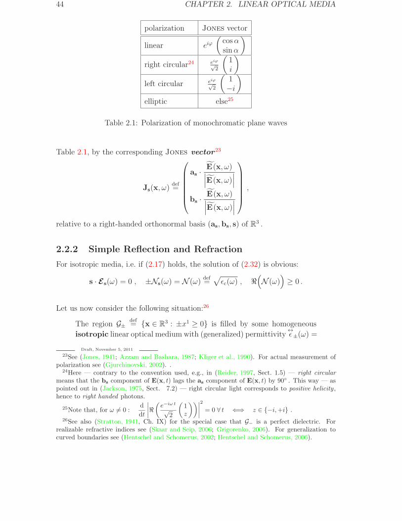
Table 2.1: Polarization of monochromatic plane waves
Table 2.1, by the corresponding Jones vector 23
Js(x, ω)def=
as ·E(x, ω)∣∣∣E(x, ω)
∣∣∣
bs ·E(x, ω)∣∣∣E(x, ω)
∣∣∣
,
relative to a right-handed orthonormal basis (as,bs, s) of R3 .
2.2.2 Simple Reflection and Refraction
For isotropic media, i.e. if (2.17) holds, the solution of (2.32) is obvious:
s · Es(ω) = 0 , ±Ns(ω) = N (ω)def=√ǫc(ω) , ℜ
(N (ω)
)≥ 0 .
Let us now consider the following situation:26
The region G±def= x ∈ R
3 : ±x1 ≥ 0 is filled by some homogeneous
isotropic linear optical medium with (generalized) permittivity↔ǫ±(ω) =
Draft, November 5, 2011
23See (Jones, 1941; Azzam and Bashara, 1987; Kliger et al., 1990). For actual measurement ofpolarization see (Gjurchinovski, 2002). .
24Here — contrary to the convention used, e.g., in (Reider, 1997, Sect. 1.5) — right circularmeans that the bs component of E(x, t) lags the as component of E(x, t) by 90 . This way — aspointed out in (Jackson, 1975, Sect. 7.2) — right circular light corresponds to positive helicity ,hence to right handed photons.
25Note that, for ω 6= 0 :d
dt
∣∣∣∣ℜ(e−iω t√
2
(1z
))∣∣∣∣2
= 0 ∀ t ⇐⇒ z ∈ −i,+i .26See also (Stratton, 1941, Ch. IX) for the special case that G− is a perfect dielectric. For
realizable refractive indices see (Skaar and Seip, 2006; Grigorenko, 2006). For generalization tocurved boundaries see (Hentschel and Schomerus, 2002; Hentschel and Schomerus, 2006).
2.2. MONOCHROMATIC WAVES OF EXPONENTIAL TYPE 45
ǫ±(ω)↔1 , and conductivity
↔σ±(ω) = σ±(ω)
↔1 . Moreover, assume
(N+(ω)
)26=(N−(ω)
)2, (2.38)
whereN±(ω)
def=√ǫ±c (ω) , ℜ
(N±(ω)
)≥ 0 .
Then scattering theory suggests to look for modes of the following form:27
• Inside G− the electric field has the form
E−(x, t) = Es− e−iω
c(c t−N−(ω) s−·x) + Es′− e−i
ωc(c t−N−(ω) s′−·x) .
• The electric field inside G+ has the form
E+(x, t) = Es+ e−iω
c(c t−N+(ω) s+·x) .
• s−, s′−, s+,Es− ,Es′− ,Es+ ∈ C3 \ 0 .
• (2.31) holds for s ∈ s−, s′−, s+ .
• s− − Pe1 s− is not isotropic28 and Pe1 s−def= (e1 · s−) e1 6= 0 .
For this Ansatz the boundary condition for the elctric field requires
e1 ×(Es− e
−i ωcN−(ω) s−·x + Es′− e
−i ωcN−(ω) s′−·x − Es+ e
−iωcN+(ω) s+·x
)|x1=0
= 0
for all x2, x3 ∈ R . This is equivalent to
e1 ×(Es−(ω) + Es′−(ω)− Es+(ω)
)= 0 (2.39)
and Snell’s law 29
e1 ×N−(ω) s′− = e1 ×N−(ω) s− = e1 ×N+(ω) s+ . (2.40)
Defining
c3def=
s− − Pe1 s−√(s− − Pe1 s−
)·(s− − Pe1 s−
) , c2def= c3 × e1
Draft, November 5, 2011
27For nonisotropic media the Ansatz has to be refined.28A vector z ∈ C
3 is called isotropic iff z · z = 0 .29Usually Snell’s law is given for the special case N±(ω) = n±(ω) ∈ R , s′−, s± ∈ R
3 . Then:
n−(ω) sin θ′− = n−(ω) sin θ− = n+(ω) sin θ+ ,
wheres± = cos θ± e1 + sin θ± e3 ; s′− = − cos θ′− e1 + sin θ′− e3 , e3
def= c3 ∈ R
3 .
46 CHAPTER 2. LINEAR OPTICAL MEDIA
we get a basis e1, c2, c3 of C3 that is orthonormal in the sense that
cj · ck = δjk , c1def= e1 .
For c3 introduced this way Snell’s law implies
s′−, s−, s+ ∈ Span e1, c3 ⊂ C3 . (2.41)
Similarly to (2.39), assuming vanishing permeability, we get
e1 ×(Bs−(ω) +Bs′−(ω)−Bs+(ω)
)= 0 . (2.42)
By (2.33) the latter is equivalent to
0 = e1 ×(N−(ω)
(s− × Es−(ω) + s′− × Es′−(ω)
)−N+(ω) s+ × Es+(ω)
). (2.43)
Thanks to (2.41) and (2.31) the splitting30
Es(ω) = E⊥s (ω) c2 + E‖
s (ω) (c2 × s) for s = s±, s′− . (2.44)
is possible iff (2.32) holds.
Proof of (2.44): Obviously, due to our assumptions concerning the material con-stants, (2.32) is equivalent to
s · Es(ω) = 0 . (2.45)
According to (2.41) and (2.31) s , c2 , c2 × s is a Basis31 of C3 . Therefore, a splittingof the form
Es(ω) = E⊥s (ω) c2 + E‖
s (ω) (c2 × s) + Eadds (ω) s
is possible. But, since s · c2 = 0 = s · (c2 × s) , Eadds (ω) vanishes iff (2.45) holds.
With this splitting, because (2.36) and (2.41) imply
e1 ×(s× (c2 × s)
)= e1 × c2 , e1 × (c2 × s) = (e1 · s) c2 ,
(2.43) becomes equivalent to
N−(ω)(E‖s−(ω) + E‖
s′−(ω))= N+(ω) E‖
s+(ω) ,
N−(ω)((e1 · s−) E⊥
s−(ω) + (e1 · s′−)E⊥s′−(ω)
)= N+(ω) (e1 · s+) E⊥
s+(ω) .
(2.46)
Similarly we see that (2.39) is equivalent to
E⊥s−(ω) + E⊥
s′−(ω) = E⊥s+(ω) ,
(e1 · s−) E‖s−(ω) + (e1 · s′−)E‖
s′−(ω) = (e1 · s+) E‖s+(ω) .
(2.47)
Draft, November 5, 2011
30The notions ⊥ and ‖ refer to the e1-c3-plane in C3 , z1 ⊥ z2 meaning z1 · z2 = 0 .
31Note that (c2 × s) · (c2 × s) = (c2 · c2) (s · s)− (c2 · s)2 = 1 .
2.2. MONOCHROMATIC WAVES OF EXPONENTIAL TYPE 47
Exercise 3 Using (2.31) and (2.41), show the following:
a) (2.47), (2.46), (2.38), and Snell’s law imply
e1 · s′− = − e1 · s− , (2.48)
if solutions with E‖s+(ω) 6= 0 as well as those with E⊥
s+(ω) 6= 0 exist.
b)s′− = (c3 · s−) c3 − (e1 · s−) e1 . (2.49)
c)
s+ =N−(ω)
N+(ω)(c3 · s−) c3 ±
√
1−(N−(ω)
N+(ω)(c3 · s−)
)2
e1 . (2.50)
By (2.48), both (2.46) and (2.47) together are equivalent to Fresnel’s formulas32
E‖s+(ω) =
2N−(ω) (e1 · s−)N−(ω) (e1 · s+) +N+(ω) (e1 · s−)
E‖s−(ω) , (2.51)
E⊥s+(ω) =
2N−(ω) (e1 · s−)N−(ω) (e1 · s−) +N+(ω) (e1 · s+)
E⊥s−(ω) , (2.52)
E‖s′−(ω) =
N+(ω) (e1 · s−)−N−(ω) (e1 · s+)N+(ω) (e1 · s−) +N−(ω) (e1 · s+)
E‖s−(ω) , (2.53)
E⊥s′−(ω) =
N−(ω) (e1 · s−)−N+(ω) (e1 · s+)N−(ω) (e1 · s−) +N+(ω) (e1 · s+)
E⊥s−(ω) . (2.54)
Exercise 4 Using Snell law, show the following:
a) (2.43) implies
e1 ·(ǫ−c (ω)Es−(ω) + ǫ−c (ω)Es′−(ω)− ǫ+c (ω)Es+(ω)
)= 0 .
b) grad (c2 · E(x, t)) is continuous.
c) grad (c3 · E(x, t)) is not continuous, in general.
Draft, November 5, 2011
32We assume that the denominators on the r.h.s. of (2.51)–(2.54) do not vanish. Forthe evaluation of these formulas in the case of nonabsorbing media and s ∈ R
3 see, e.g.,(Monzon and Sanchez-Soto, 2001).
48 CHAPTER 2. LINEAR OPTICAL MEDIA
Let us consider the case33
ℜ (e1 · s±) > 0 . (2.55)
Then Es− e−iω
c(c t−N−(ω) s−·x) may be interpreted as incoming wave,34 reflected into
G− as Es′− e−iω
c(c t−N−(ω) s′−·x) and transmitted into G+ as Es+ e
−iωc(c t−N+(ω) s+·x) .
As a direct consequence of (2.37) we have
e1 ·⟨Ss−(x, t)
⟩|x1=0
= e1 ·⟨S⊥s−(x, t)
⟩|x1=0
+ e1 ·⟨S ‖s−(x, t)
⟩|x1=0
,
where35
Ss−(x, t)def= Poynting vector of Es± e
−iωc(c t−N−(ω) s−·x) ,
S⊥s−(x, t)
def= Poyn<ting vector of E⊥
s−c2 e−iω
c(c t−N−(ω) s−·x) ,
S‖s−(x, t)
def= Poynting vector of E ‖
s−(c2 × s−) e−iω
c(c t−N−(ω) s−·x) .
Since, similar relations hold for s′− and s+ instead of s− , we may analyze the energyflow for the ⊥- and ‖-modes separately. Let us define
R⊥s−(ω)
def= −
e1 ·⟨S⊥s′−(x, t)
⟩|x1=0
e1 ·⟨S⊥s−(x, t)
⟩|x1=0
,
T⊥s−(ω)
def= +
e1 ·⟨S⊥s+(x, t)
⟩|x1=0
e1 ·⟨S⊥s−(x, t)
⟩|x1=0
for e1 ·⟨S⊥s−(x, t)
⟩|x1=0
6= 0
and similarly for ‖ instead of ⊥ . Then by (2.37) and Snell’s law (2.40) we have
R⊥s−(ω) = − e1 · ℜ(N−(ω)s′−)
e1 · ℜ(N−(ω)s−)
∣∣E⊥s′−(ω)
∣∣2/∣∣E⊥
s−(ω)∣∣2
=(2.48),(2.54)
∣∣∣∣N−(ω) (e1 · s−)−N+(ω) (e1 · s+)N−(ω) (e1 · s−) +N+(ω) (e1 · s+)
∣∣∣∣2
(2.56)
and
T⊥s−(ω) = +
e1 · ℜ(N+(ω)s+)
e1 · ℜ(N−(ω)s−)
∣∣E⊥s+(ω)∣∣2/∣∣E⊥
s−(ω)∣∣2
=(2.53)
ℜ(N+(ω) (e1 · s+)
)
ℜ(N−(ω) (e1 · s−)
)∣∣∣∣
2N−(ω) (e1 · s−)N−(ω) (e1 · s−) +N+(ω) (e1 · s+)
∣∣∣∣2
.(2.57)
Draft, November 5, 2011
33For ℜ (e1 · s+) < 0 we have incoming waves from both sides of the boundary.34Actually we should form wave packets by integrating with suitable weights over s− and ω .35Recall (2.44).
2.2. MONOCHROMATIC WAVES OF EXPONENTIAL TYPE 49
Therefore36
R⊥s−(ω) + T⊥
s−(ω) = 1
⇐⇒ℜ(N+(ω) (e1 · s+)
)
ℜ(N−(ω) (e1 · s−)
) = ℜ(N+(ω) (e1 · s+)N−(ω) (e1 · s−)
)
⇐⇒N−(ω) (e1 · s−) , N+(ω) (e1 · s+)N−(ω) (e1 · s−)
∩ R 6= ∅ ,
i.e.:
In general, the usual interpretation of R⊥s−(ω) as reflectance and T⊥
s−(ω)
as transmittance (of the ⊥-mode) is not strictly justified.
For the ‖-mode the situation is more complicated, since, e.g.,37
ℜ(N−(ω)
(Es−(ω) · s−
)Es−(ω)
)= i c2 · (s− × s−)ℑ
(N−(ω) E ‖
s−(ω)Es−(ω)).
The latter, however, implies
e1·ℜ(N−(ω)
(Es−(ω) · s−
)Es−(ω)
)= i c2·(s− × s−)
∣∣E ‖s−(ω)
∣∣2 ℑ(N−(ω) (c3 · s−)
).
(2.58)and, therefore, similarly to (2.56) and (2.57) we get
ℑ(N−(ω) (c3 · s−)
)(s− × s−) = ℑ
(N+(ω) (c3 · s+)
)(s+ × s+) = 0
=⇒ R ‖s−(ω) =
∣∣∣∣N+(ω) (e1 · s−)−N−(ω) (e1 · s+)N+(ω) (e1 · s−) +N−(ω) (e1 · s+)
∣∣∣∣2
(2.59)
and
ℑ(N−(ω) (c3 · s−)
)(s− × s−) = ℑ
(N+(ω) (c3 · s+)
)(s+ × s+) = 0
=⇒ T ‖s−(ω) =
ℜ(N+(ω) (e1 · s+)
)
ℜ(N−(ω) (e1 · s−)
)∣∣∣∣
2N−(ω) (e1 · s−)N−(ω) (e1 · s+) +N+(ω) (e1 · s−)
∣∣∣∣2
.(2.60)
Draft, November 5, 2011
36Note that
ℜ(z+)ℜ(z−)
= ℜ(z+z−
)⇐⇒ z+ z− (z− − z−) = z+ z− (z− − z−) .
For a discussion of the reflection and transmission in the case of normal incidence see(Lodenquai, 1991).
37Note that, e.g.,
i c2 · (s− × s−) = 2αβ for s− = α e1 + i β c3 α, β ∈ R .
50 CHAPTER 2. LINEAR OPTICAL MEDIA
Warning: Note that (2.56), (2.57), (2.59), and (2.60) hold only for
ℜ(N−(ω) (e1 · s−)
)6= 0 .
A direct consequence of (2.57) is that ℜ(N+(ω) (e1 · s+)
)= 0 implies T⊥
s−(ω) = 0 ,
i.e. total reflection of the ⊥-mode.38 If, in addition,
ℑ(N−(ω) (c3 · s−)
)(s− × s−) = ℑ
(N+(ω) (c3 · s+)
)(s+ × s+) = 0
holds then, by (2.60), also T‖s−(ω) = 0 .
Strictly speaking, however, total reflection appears only since G+ has infinitediameter. If G+ is replaced by a layer of finite depth, then optical tunneling ispossible, i.e. partial transmission of radiation under the conditions of otherwise totalreflection. Then, however, there is a superposition of two evanescent modes insideG+ with non-vanishing e1-component of the total Poynting vector.39
Remarks:
1. Multiple total reflection may be used for building useful opticaldevices (e.g. wave guides).
2. In case of total reflection the evanescent wave inside G+ has higherspatial frequency (=higher resolution) in the direction of propa-gation than usual and may have considerable amplitudes near theboundary of the media. These modes are exploited by near-fieldscanning optical microscopy40 (NSOM), converting the evanescentmodes into propagating ones.
3. Usually scattered light contains evanescent near-field components(Wolf and Nieto-Vesperinas, 1985).
4. Optical tunneling may be used for coupling wave guides.
Exercise 5 For real N±(ω) = N±(ω) = n±(ω) and s− ∈ R3 show that R
‖s−(ω)
vanishes iff(e1 · s−)2
1− (e1 · s−)2=
(n−(ω
n+(ω)
)2
,
Draft, November 5, 2011
38Usually the case
N±(ω) = n±(ω) , n−(ω) sin θ− > n+(ω) , s− ∈ R3
is considered, corresponding to total reflection since the e1-component of (2.50) becomes purelyimaginary.
39And the results for incident monochromatic plane waves should not be applied too naively toalmost monochromatic incident rays!
40See, e.g., (Ohtsu and Hori, 1999) and (Paesler and Moyer, 1996).
2.2. MONOCHROMATIC WAVES OF EXPONENTIAL TYPE 51
i.e. iff ∠e1, s− coincides with the so-called Brewster angle arctann−(ω)
n+(ω). More-
over, show that in this case
R ‖s−(ω) = 0 ⇐⇒ s′− · s+ = 0 .
2.2.3 Birefringent Media (Crystal Optics)
Generally, (2.32) is equivalent to
↔M s(ω)Es(ω) = 0 , (2.61)
where↔M s(ω)
def=(Ns(ω)
)2↔1 −
s1s1 s1s2 s1s3
s2s1 s2s2 s2s3
s3s1 s3s2 s3s3
− ↔
ǫc(ω) .
(2.61) can be fulfilled iff
det(↔M s(ω)
)= 0 . (2.62)
Therefore, we have to choose the complex refractive index Ns(ω) such that(2.62) is fulfilled and determine the (complex) direction of Es(ω) from (2.32) forsuch Ns(ω) .
Reasonable physical assumptions imply that41
a · ↔ǫ c(ω)b = b · ↔ǫ c(ω) a ∀ a,b ∈ C3 . (2.63)
Therefore, if Ns(ω) resp. N ′s(ω) are solutions of (2.62) and Es(ω) resp. E
′
s(ω) cor-responding solutions of (2.32), we have
(Ns(ω)
)26=(N ′
s(ω))2
=⇒(↔ǫ c(ω)Es(ω)
)· ↔ǫ c(ω)E ′
s(ω) = 0 . (2.64)
Proof of (2.64):
(N ′
s(ω))2 (↔
ǫ c(ω)Es(ω))· ↔ǫ c(ω)E
′
s(ω)
=(2.32)
(Ns(ω))2 (N ′
s(ω))4 ↔P⊥s Es(ω) ·
↔P⊥s E
′
s(ω)
= (Ns(ω))2 (N ′
s(ω))4
Es(ω) ·↔P⊥s E
′
s(ω)
=(2.32)
(Ns(ω)N ′s(ω))
2Es(ω) ·
↔ǫ c(ω)E
′
s(ω)
=(2.63)
(Ns(ω)N ′s(ω))
2E ′
s(ω) ·↔ǫ c(ω)Es(ω)
=(2.32)
(Ns(ω)
)2 (↔ǫ c(ω)E
′
s(ω))· ↔ǫ c(ω)Es(ω) .
Draft, November 5, 2011
41See (Romer, 1994, Ends of Sections 2.4 and 2.7).
52 CHAPTER 2. LINEAR OPTICAL MEDIA
Because ofa · b = b · a ∀a,b ∈ C
3
this implies
((Ns(ω)
)2−(N ′
s(ω))2)(↔
ǫ c(ω)Es(ω))· ↔ǫ c(ω)E
′
s(ω) = 0
and hence (2.64).
Note that (2.64), (2.32), and (2.31) imply
(Ns(ω)
)26=(N ′
s(ω))2
=⇒ Es(ω) · E ′
s(ω) = (s · Es(ω)) (s · E ′
s(ω)) . (2.65)
s is said to correspond to an optical axis for given ω , if there is a uniquecomplex refractive index Ns(ω) = N ord
s (ω) for which there are two independentsolutions Es(ω) of (2.32).
Lemma 2.2.1 s corresponds to an optical axis for given ω iff
s · e = 0 =⇒ e ·(↔ǫ c(ω)
)−1
e =(N ord
s (ω))−2
(2.66)
holds for all (complex) directions e .
Proof: Let s correspond to an optical axis and let Es(ω),E′
s(ω) be independentsolutions of (2.32) for Ns(ω) = N ord
s (ω) . Then, because of
Es(ω) =(N ord
s (ω))2 (↔
ǫ c(ω))−1↔
P⊥s Es(ω) , (2.67)
(and the corresponding equation for E ′
s(ω)) also↔P⊥s Es(ω) and
↔P⊥s E
′
s(ω) have tobe independent. Moreover, (2.67) implies
(↔P⊥s Es(ω)
)=(N ord
s (ω))2 ↔
I s
(↔P⊥s Es(ω)
)
for↔I s
def=
↔P⊥s
(↔ǫ c(ω)
)−1↔P⊥s .
Therefore,↔I s =
1
(N ords (ω))
2
↔P⊥s .
Since
s · e = 0 ⇐⇒ e =↔P⊥s e
and
a ·(
↔P⊥s b
)=
(↔P⊥s a
)· b ∀a,b ∈ C
3 ,
2.2. MONOCHROMATIC WAVES OF EXPONENTIAL TYPE 53
we conclude42 that (2.66) holds. Conversely, if (2.66) holds, then
Es(ω) =(↔ǫ c(ω)
)−1
z
is a solution of (2.32) for every z ∈↔P⊥s C
3 . The latter shows that s corresponds toan optical axis.
Let us assume that↔ǫ c(ω) may be diagonalized:
↔ǫ c(ω) =
ǫ1c(ω) 0 00 ǫ2c(ω) 00 0 ǫ3c(ω)
w.r.t. z1(ω), z2(ω), z3(ω) ⊂ C
3 ,
zj(ω) · zk(ω) = δjk ∀ j, k ∈ 1, 2, 3 .(2.68)
Remark: (2.68) is guaranteed by (2.63), for suitable zj(ω) ∈ C3, if
↔ǫ c(ω) does not
have any isotropic eigenvector; see Lemma 7.4.13 of (Lucke, eine). Note, however,that there are media (monoclinic and triclinic crystals) for which the eigenvectors of↔ǫ c(ω) depend on ω .
If (2.68) holds with ǫ2c(ω) = ǫ3c(ω) , then ±z1(ω) corresponds to an optical axis and
N ordz1(ω)
(ω) =√ǫ2c(ω) . (2.69)
In this case, whenever s 6∼ z1(ω) ,
Es(ω) = Eords (ω) ∼ s× z1(ω) , (2.70)
is a solution of (2.32) forNs(ω) = N ord
z1(ω)(ω) .
Note that, by (2.37),s ∈ R =⇒
⟨Sords (x, t)
⟩∼ s . (2.71)
To determine the second solution of (2.62) we may assume, without loss of generality,that
s = s1(ω) z1(ω) + s3(ω) z3(ω) .
Then, w.r.t. z1(ω), z2(ω), z3(ω) , by (2.31), we have
↔M(k0) =
(Ns(ω)
)2
+s3(ω)s3(ω) 0 −s1(ω)s3(ω)0 1 0
− s3(ω)s1(ω) 0 +s1(ω)s1(ω)
− ↔
ǫc(ω)
Draft, November 5, 2011
42Recall that↔P⊥s
↔P⊥s =
↔P⊥s .
54 CHAPTER 2. LINEAR OPTICAL MEDIA
and hence (2.62) holds iff either Ns(ω) = N ordz1(ω)
(ω) or
0 =((
Ns(ω))2s3(ω)s3(ω)− ǫ1c(ω)
)((Ns(ω)
)2s1(ω)s1(ω)− ǫ3c(ω)
)
−(Ns(ω)
)4s1(ω)s1(ω)s3(ω)s3(ω)
= ǫ1c(ω) ǫ3c(ω)
(1− (Ns(ω) s
1(ω))2
ǫ3c(ω)− (Ns(ω) s
3(ω))2
ǫ1c(ω)
).
Therefore another solution E ′
s(ω) of (2.32) exists for Ns(ω) = N exos (ω) , the latter
being implicitly defined by
(N exos (ω) s1(ω)
N ords (ω)
)2
+
(N exo
s (ω) s2(ω)√ǫ1c(ω)
)2
+
(N exo
s (ω) s3(ω)√ǫ1c(ω)
)2
= 1 . (2.72)
In the nonisotropic case, (2.70) and (2.64) imply
Eexos (ω) ∼
(↔ǫ c(ω)
)−1(s×
(s× z1(ω)
)). (2.73)
In agreement with (2.65) we have Eexos (ω) · Eord
s (ω) = 0 , in the present case.43
Exercise 6 Show that
Eords (ω) ·
⟨Sords (x, t)
⟩= E
exos (ω) · 〈Sexo
s (x, t)〉 = 0
and〈Sexo
s (x, t)〉 ∈ Span s,Eexos (ω) ⊂ Span
s, z1(ω)
if z1(ω) 6∼ s ∈ R3 and
↔ǫc =
(↔ǫc
)†.
Remarks:
1. For real directions e and real↔ǫ c(ω) we have
(↔ǫ c(ω)
)−1
e =1
2
(∇x
(x ·(↔ǫ c(ω)
)−1
x))
|x=e
and, therefore,(↔ǫ c(ω)
)−1
e ∼ n(e) , where n(e) denotes the nor-
mal of the index ellipsoidx ∈ R :
(x ·(↔ǫ c(ω)
)−1
x
)= 1
at x ∼ e .
Draft, November 5, 2011
43Note that, in the present case,(↔ǫ c(ω)
)−1
leaves the linear span of s and z1(ω) invariant.
2.2. MONOCHROMATIC WAVES OF EXPONENTIAL TYPE 55
2. Since, therefore, s · Eexos (ω)
i.g.
6= 0 Exercise 6 and (2.71) show that
〈Sexos (x, t)〉
i.g.
6∼ s ∼⟨Sords (x, t)
⟩;
i.e. the medium is birefringent .
Lemma 2.2.2 If (2.68) holds with ǫ1c(ω) 6= ǫ2c(ω) and if s is a (complex) direction
corresponding to an optical axis for given ω then3∏
j=1
s · zj(ω) = 0 .
Outline of proof: Let s correspond to an optical axis. Then, by Lemma 2.2.1,
s · x = 0 6= x · x =⇒3∑
j=1
(xj)2/ǫjc = C x · x ∀x ∈ C3
holds for some C = C(ω) ∈ C , where xjdef= x · zj(ω) for j = 1, 2, 3 . Now assume∏3
j=1 sj 6= 0 . Then
s · x = 0 ⇐⇒(x1)2
=
(s2x2 + s3x3
s1
)2
and, therefore, we have
(s2x2 + s3x3
s1
)2
+(x2)2
+(x3)2 6= 0
=⇒ 1
ǫ1c
(s2x2 + s3x3
s1
)2
+1
ǫ2c
(x2)2
+1
ǫ3c
(x3)2
= C
((s2x2 + s3x3
s1
)2
+(x2)2
+(x3)2)
for all x2, x3 ∈ C . Comparing the x2x3-terms on both sides of the latter equationshows that C = 1/ǫ1c . Similarly we conclude that C = 1/ǫ2c . Therefore,
∏3j=1 s
j 6= 0
cannot hold if ǫ1c 6= ǫ2c .
Corollary 2.2.3 If (2.68) holds with ǫ1c(ω) 6= ǫ2c(ω) and if s is a (complex) directionwith s · z2(ω) = 0, for given ω , then s corresponds to an optical axis if and only ifǫ1c(ω) 6= ǫ3c(ω) and
s = ±√1− (s3)2 z1(ω) + s3 z3(ω) , s3 = ±
√ǫ3c(ω)− ǫ2c(ω)
ǫ3c(ω)− ǫ1c(ω)
ǫ1c(ω)
ǫ2c(ω). (2.74)
56 CHAPTER 2. LINEAR OPTICAL MEDIA
Outline of proof: Let the direction s ⊥ z2(ω) correspond to an optical axis. Thenthere are complex numbers C and s3 with
s = ±√
1− (s1)2z1(ω) + s3 z3(ω)
and
s · s′ = 0 =⇒ s′ ·(↔ǫ c(ω)
)−1
s′ = C
for all directions s′ (by Lemma 2.2.1). Especially for
edef= z2(ω) , e′
def= s3 z1(ω)∓
√1− (s1)
2z3(ω) ,
therefore, we have
1/ǫ2c = e ·(↔ǫ c(ω)
)−1
e
= e′ ·(↔ǫ c(ω)
)−1
e′
=
(s3)2
ǫ1c+
1−(s3)2
ǫ3c.
This implies ǫ1c 6= ǫ3c (since ǫ1c 6= ǫ2c , by assumption) and (2.74). Conversely, since
e ·(↔ǫ c(ω)
)−1
e′ = 0 , it is obvious (by Lemma 2.2.1) that s corresponds to an optical
axis under these conditions.
Remarks:
1. For the caseǫ1c(ω) 6= ǫ2c(ω) = ǫ3c(ω) , (2.75)
Lemma 2.2.2 and Corollary 2.2.3 show that only ±z1(ω) corre-sponds to an optical axis. Therefore media for which (2.68) and(2.75) hold are called uniaxial .
2. Media withǫ1c(ω) 6= ǫ2c(ω) 6= ǫ3c(ω) 6= ǫ1c(ω)
are called biaxial . Actually, by Corollary 2.2.3, there are 6 opticalaxes,44 but only those corresponding to ‘sufficiently real’ directionsare relevant for physical applications.
3. For biaxial media with
ǫ3c(ω) > ǫ2c(ω) > ǫ1c(ω) > 0 (2.76)
the real directions e corresponding to optical axes are given byCorollary 2.2.3 (for the choice of indices corresponding to (2.76)).
4. Crystals of the hexagonal, tetragonal and trigonal system are uniax-ial and the optical axis coincides with the crystal axis of six-, four-,or three-fold symmetry. Crystals of the orthorhombic, monoclinicand triclinic system are optically biaxial.
Draft, November 5, 2011
44Note that the choice of indices in (2.68) is arbitrary
2.3. MONOCHROMATIC LIGHT RAYS 57
2.3 Monochromatic Light Rays45
In this section we consider only isotropic media and — in order to be able to applystandard Fourier analysis (for tempered distributions) — only the case46
N (ω) = n(ω) > 0 .
Then, by monochromatic light ray we mean a solution of Maxwell’s equationsfulfilling the following two conditions for suitable ω and s ∈ R
3 with |s| = 1 :
1. E(x, t) = E(x) e−i ω t(i.e. : E(x, ω′) = E(x) δ(ω′ − ω)
).
2.∣∣E(k)
∣∣≪ 1 unless |k|2 − (s · k)2 ≪ |k|2 ,where
E(k)def= (2π)−3/2
∫E(x) eix·k dVx . (2.77)
Let us assume s = e3 and define
F(k1, k2; x3)def= e−i
ωcn(ω)x3 1
2π
∫E(x) e−i(x
1k1+x2k2) dx1dx2 .
Then the Helmholtz equation (2.29) gives47
(−(k1)2 −
(k2)2
+
(∂
∂x3
)2
+(ωcn(ω)
)2)(
e+iωcn(ω)x3
F(k1, k2; x3))= 0 .
Since48
(∂
∂x3
)2 (e+i
ωcn(ω)x3
F(k1, k2; x3))
= e+iωcn(ω)x3
(−(ωcn(ω)
)2+ 2 i
ω
cn(ω)
∂
∂x3+
(∂
∂x3
)2)F(k1, k2; x3)
≈ e+iωcn(ω)x3
(−(ωcn(ω)
)2+ 2 i
ω
cn(ω)
∂
∂x3
)F(k1, k2; x3) ,
we conclude:((k1)2
+(k2)2 − 2 i
ω
cn(ω)
∂
∂x3
)F(k1, k2; x3) ≈ 0 . (2.78)
Draft, November 5, 2011
45See also (Gomez-Reino et al., 2002).46Recall (2.30).47Recall that, in the isotropic case, (2.29) implies div E(x, ω) = 0 .
48Thanks to the second defining condition for light rays , we may neglect
(∂
∂x3
)2
F(k1, k2;x3) .
58 CHAPTER 2. LINEAR OPTICAL MEDIA
This justifies to approximate F(k1, k2; x3) by the unique solution49
F≈(k1, k2; x3) = e
−i (k1)2+(k2)2
2 ωc n(ω)
x3
F(k1, k2; 0) (2.79)
of the initial-value problem
∂
∂x3F≈(k
1, k2; x3) =(k1)2 + (k2)2
2 i ωcn(ω)
F≈(k1, k2; x3) ,
F≈(k1, k2; 0) = F(k1, k2; 0) =
1
2π
∫E(x1, x2, 0) e−i(x
1k1+x2k2) dx1dx2 .
Because of
E(x) =1
2π
∫e+i
ωcn(ω)x3
F(k1, k2; x3) e+i(x1k1+x2k2) dk1 dk2 (2.80)
this means:
E(x) ≈ (2π)−2
∫ (∫E(x1, x2, 0) e−i(x
1k1+x2k2) dx1dx2)·
· e−i(k1)2+(k2)2
2 ωc n(ω)
x3
e+i(x1k1+x2k2) dk1dk2 .
(2.81)
Hence:
For monochromatic light rays,50 E(x) can be calculated everywhere ap-proximately from its values on any plane that is perpendicular to thepropagation direction s .
Especially for (linearly polarized) Gaussian rays , characterized (up to spatialrotation and translation) by
E(x)|x3=0
= E0 exp
(−(x1)
2+ (x2)
2
δ2
), s = e3 ,
Draft, November 5, 2011
49We skip the detailed mathematical prove of uniqueness.50We do not elaborate on which profiles E(x)|x3=0
are actually possible for monochromatic lightrays.
2.4. GROUP-VELOCITY DISPERSION 59
(2.81) gives
E(x) ≈ (2π)−2E0
∫ (∫e−
(x1)2+(x2)
2
δ2 e−i(x1k1+x2k2) dx1dx2
)·
· e−i(k1)2+(k2)2
2 ωc n(ω)
x3
e+i(x1k1+x2k2) dk1dk2
=δ2
4πE0
∫e−((k1)
2+(k2)
2)δ2/4
e−i (k1)2+(k2)2
2 ωc n(ω)
x3
e+i(x1k1+x2k2) dk1dk2
=δ2
4πE0
2∏
j=1
∫exp
(−(kR(x3)
)2+ i xj k
)dk
=δ2
4πE0
2∏
j=1
(e−(
xj
2R(x3)
)2 ∫exp
(−(kR(x3)− i
xj
2R(x3)
)2)dk
)
=
(δ
2R(x3)
)2
exp
(−(
x1
2R(x3)
)2
−(
x2
2R(x3)
)2),
where
R(x3)def=
√(δ/2)2 + i
x3
2 ωcn(ω)
, ℜ(R(x3)
)> 0 ,
since
ℜ(R2)> 0 < ℜ(R) =⇒
∫ +∞
−∞e−(Rx+z0)2 dx =
√π
R ∀R , z0 ∈ C (2.82)
(see, e.g., Sect. 2.1.3 of (Lucke, ftm) for a proof of (2.82)) and hence
1√2π
∫e−x
2
e−i x k dx =1√2e−k
2/4 ∀ k ∈ R . (2.83)
2.4 Group-Velocity Dispersion
See (Reider, 1997, Sect. 3.2.1).

60 CHAPTER 2. LINEAR OPTICAL MEDIA
Chapter 3
Nonlinear Optical Media
3.1 General Considerations
If, in Exercise 1, the damped harmonic oscillator is replaced by ananharmonic one then its evolution depends nonlinearly on the drivingforce. As a consequence — even if the driving force is monochromatic —higher harmonics show up in the motion of the oscillator; mainly secondorder harmonics if the medium is not inversion symmetric1 (compare(Reider, 1997, Sect. 8.1)). Moreover, if the driving force is a superpo-sition of two monochromatic ones, the motion of the oscillator containsharmonic components corresponding to the sum as well as to the differ-ence of both frequencies.2
If the damped harmonic oscillator model is applied to the electric dipolesof an optical medium then the accelerated charge of the dipoles createa radiation field acting on the other charges in addition. Therefore,actually, the driving field is a superposition of the incident exterior fieldwith the radiation emitted from the medium’s electric dipoles. Now,if the harmonic oscillator is replaced by a more realistic nonlinear one,then the radiation contributed by the medium itself (to the macroscopicelectromagnetic field) contains higher harmonics of every monochromaticcomponent of the incident (microscopic) field as well as components withfrequencies corresponding to the sum or difference of any two frequenciespresent in the incident field.
Usually, very strong electromagnetic fields — as provided by laser pulsesof high intensity — or long optical path length’s in low-loss nonlinearoptical media (optical fibers, see (Agrawal, 1999, Sect. 1.3.3)) — have tobe applied in order to gain recognizable nonlinear effects. Then, however,
Draft, November 5, 2011
1Since, e.g., silicia glasses — the material of choice for low-loss optical fibers, formed by fusingSiO2 molecules — are inversion symmetric they do not normally exhibit second-order nonlineareffects.
2See (Mills, 1998, Sect. 3.1) for a perturbative calculation.
61
62 CHAPTER 3. NONLINEAR OPTICAL MEDIA
interesting phenomena show up several of which will be studied in thischapter.
3.1.1 Functionals of the Electric Field
Usually, especially in optical applications, P(x, t) is assumed to be a (sufficientlywell-behaved) functional of E . Then3 we have the functional Taylor expansion4
Pj(x, t) =∞∑
ν=0
P (ν)j (x, t) , (3.1)
P (ν)j (x, t) =
ǫ0
(2π)ν2
∫χ(ν)jk1...kν
(x, t;x′1, t
′1; . . . ;x
′ν , t
′ν)E
k1(x′1, t
′1) . . .
. . . Ekν (x′ν , t
′ν) dVx′
1 dt′1 . . . dVx′
νdt′ν ,
(3.2)
w.r.t. an arbitrary Basis b1,b2,b3 of R , where5
Pj(x, t) def= bj ·P(x, t) , Ek(x′, t′)
def= bk · E(x, t) .
Note that the coefficients χ(ν) fulfill the symmetry condition6
χ(ν)jk1...kν
(x, t;x′1, t
′1; . . . ;x
′ν , t
′ν) = χ
(ν)jkπ(1)...kπ(ν)
(x, t;x′π(1), t
′π(1); . . . ;x
′π(ν), t
′π(ν)) (3.3)
for every permutation π of (1, . . . , ν) . If, in addition, we assume homogeneity inspace and time these coefficients have to be of the form
χ(ν)jk1...kν
(x, t;x′1, t
′1; . . . ;x
′ν , t
′ν) = χ
(ν)jk1...kν
(x− x′1, t− t′1; . . . ;x− x′
ν , t− t′ν) .
Assuming, moreover, spatial nonlocality of the electric field contributions to benegligible we have
χ(ν)jk1...kν
(x, t;x′1, t
′1; . . . ;x
′ν , t
′ν) = χ
(ν)jk1...kν
(t− t′1, . . . , t− t′ν) δ(x− x′1) . . . δ(x− x′
ν) .
Thus,
(2π)ν−12
ǫ0P (ν)j (x, t)
=1√2π
∫χ(ν)jk1...kν
(ω1, . . . , ων) Ek1(x, ω1) . . . E
kν(x, ων) e
−i(ω1+...+ων)t dω1 . . . dων
(3.4)
Draft, November 5, 2011
3See Appendix A.1.
4We use Einstein’s summation convention meaning, e.g., χjk Ek ≡
3∑
k=1
χjk Ek .
5Recall that the reciprocal basisb1,b2,b3
is characterized by:
bj · bk =1 for j = k ,0 else .
6Recall (A.1).
3.1. GENERAL CONSIDERATIONS 63
holds for the (generalized) susceptibilities
χ(ν)jk1...kν
(ω1, . . . , ων)def= (2π)−
n2
∫χ(ν)jk1...kν
(t1, . . . , tν) ei(ω1 t1+...+ων tν) dt1 . . . dtν
and (3.3) is equivalent to
χ(ν)jk1...kν
(ω1, . . . , ων) = χ(ν)jkπ(1)...kπ(ν)
(ωπ(1), . . . , ωπ(ν)) . (3.5)
The Fourier transform of (3.4) is7
(2π)ν−12
ǫ0P (ν)j (x, ω)
=
∫χ(ν)jk1...kν
(ω1, . . . , ων) Ek1(x, ω1) . . . E
kν(x, ων) δ (ω1 + . . .+ ων − ω) dω1 . . . dων .
(3.6)An optical medium modeled by (3.6) is called a linear optical medium if all the
nonlinear susceptibilities χ(ν)jk1...kν
(ω1, . . . , ων) , ν > 1 , vanish.8
Usually,P(x, t) = Pel(x, t)
is assumed for optical media and the susceptibilities should be caculated by (time-
dependent) quantum mechnical perturbation theory.9 For the tensor χ(1)jk(ω) of the
linear susceptibility first order perturbation theory is sufficient.
3.1.2 Various Electric Polarization Effects
See (Romer, 1994, Chapter 5).
3.1.3 Perturbative Solution of Maxwell’s Equations
If we replace P by P (1) in (2.1) and↔χ by
↔χ(1)
in the definition of the permit-
tivity↔ǫ then the Fourier transformed Maxwell equations (1.18)–(1.21) become
equivalent to:
curl H(x, ω) = −i ω ǫ0↔ǫ (ω) E(x, ω) + ex(x, ω)− i ω P
nl(x, ω) , (3.7)
curl B(x, ω) = i ω H(x, ω) , (3.8)
div(ǫ0
↔ǫ (ω) E(x, ω)
)= ρex(x, ω)− div
(P
nl(x, ω)), (3.9)
div B(x, ω) = 0 , (3.10)
Draft, November 5, 2011
7For a listing of the dependence of the lowest nonlinear susceptibilities on the symmetry classesfor crystals see (Brunner and Junge, 1982, Sect. 3.2.2.1).
8Note that nonlinearity does not necessarily mean that χ(ν)jk1...kν
(ω, . . . , ω) 6= 0 for some ν > 1 .9See (Armstrong et al., 1962a).
64 CHAPTER 3. NONLINEAR OPTICAL MEDIA
whereP
nl(x, ω)def= P(x, ω)− P (1)
j (x, ω)bj .
Now we have to replace (2.12) by the nonlinear equation10
HE(x, ω) = −i ω µ0 cr(x, ω)− ω2µ0 Pnl(x, ω; E (x, .)
)(3.11)
in which we have written Pnl(x, ω; E (x, .)
)instead of Pnl(x, ω) in order to indi-
cate the functional (nonlinear) dependence on E (x, .) , determined by the nonlinearsusceptibilities, and where
H E(x, ω)def=
(∆x +
(ωc
)2↔ǫ c(ω)
)E(x, ω)− grad
(div E(x, ω)
). (3.12)
Motivated by the results of 2.1.3, let us assume that there is a unique (matrix-valued,
restarted) response function↔r (x, t) of the corresponding linear medium such that
R(x, t; )def=
1√2π
∫↔r (x− x′, t− t′) (x′, t′) dVx′ dt′ (3.13)
fulfills the conditions
(x, t) = 0 for (|x| , t) /∈ [0,+R]× [0,+∞)
=⇒ R(x, t; ) = 0 for t /∈[0, |x|−R
c
]
andH R(x, ω; ) = −i ω µ0 (x, ω) (3.14)
for all sufficiently well-behaved , where
R(x, ω; )def=
1√2π
∫R(x, t; ) e+i ω t dt
=
∫↔r (x− x′, ω) (x′, ω) dVx′ . (3.15)
Let us only consider the case
cr = 0 .
Then E(x, ω) is a solution of (3.11) iff the linear equation
H E0(x, ω) = 0 . (3.16)
Draft, November 5, 2011
10Again, (3.9) serves as a definition of ρex(x, ω) for ω 6= 0 .
3.2. CLASSICAL NONLINEAR OPTICAL EFFECTS 65
is fulfilled forE0(x, ω) = E(x, ω)− R
(x, ω;
E
),
whereE(x, ω)
def= −iω P
nl(x, ω; E (x, .)
). (3.17)
This suggests the following perturbative solution of (3.11):
Take a solution E0(x, ω) of (3.16) and define recursively
Eν(x, ω)def= E0(x, ω) + R
(x, ω;
Eν−1
)for ν = 1, 2, 3, . . .
(compare Section 5.1.3 von (Lucke, ein)). Then
E(x, ω) = limν→∞
Eν(x, ω) ,
if the limit exists (in a suitable topology), is a solution of (3.11).
Certainly, one will try to get along with the first order approximation
E(x, ω) ≈ E0(x, ω)− iω
∫↔r (x− x′, ω) Pnl
(x′, ω; E 0(x
′, .))dVx′ (3.18)
(for properly chosen E0(x, ω)) as far as possible. Note that, by (3.11)–(3.13), wehave
H E(x, ω) = −ω2µ0 Pnl(x, ω; E 0(x, .)
)(3.19)
in this approximation.
3.2 Classical Nonlinear Optical Effects11
3.2.1 Phase Matching
Let us discuss the approximations (3.18) and
Pnlj (x, ω) ≈ P (2)
j (x, ω) =(3.6)
∫χ(2)jkl(ω
′, ω − ω′) Ek(x, ω′) E
l(x, ω − ω′) dω′ . (3.20)
By (3.19), then, we have to expect that
ω = ω1 + ω2 ,
χ(2)jkl(ω1, ω2) E
k0 (x, ω1) E
l0(x, ω1) 6= 0
for suitable ω1, ω1 ∈ R
=⇒ E(x, ω) 6= 0
Draft, November 5, 2011
11A freeware program for calculating nonlinear frequency conversion processes is offered at:www.sandia.gov/imrl/XWEB1128/xxtal.htm
66 CHAPTER 3. NONLINEAR OPTICAL MEDIA
and hence(E 0(x, ω1) 6= 0 6= E 0(x, ω2) =⇒ E (x, ω1 + ω2) 6= 0
)∀ω1, ω2 ∈ R
holds for sufficiently nontrivial12 χ(2) . Especially for ω1 = ω2 this means secondharmonic generation . Of course, the crucial question is how strong these effectsare.
Actually, as can be explained by simple models, Miller’s rule 13
∆jkl(ω1, ω2)def=
χ(2)jkl(ω1, ω2)
χ(1)jj (ω1 + ω2)χ
(1)kk (ω1)χ
(1)ll (ω2)
≈ independent of ω1, ω2 , (3.21)
w.r.t. the principal directions in the medium, is valid for a large variety of crystals.Therefore the dispersion relations14 for the linear susceptibilities χ
(1)jk , qualitatively
described by Exercise 1, are of great importance also for the second order suscepti-bilities.
Let us analyze (3.18)/(3.19) for the special case that the solution E0(x, ω) of(3.16) is of the form15
E0(x, ω) = E0(x, ω)(δ(ω1 − ω) + δ(ω2 − ω)
)
+E0(x,−ω)(δ(ω1 + ω) + δ(ω2 + ω)
).
(3.22)
Then we have
Ek
0 (x, ω′) E
l
0(x, ω − ω′)
= Ek0 (x, ω′) E l0(x, ω − ω′)(δ(ω1 − ω′) + δ(ω2 − ω′)
)(δ(ω1 − ω + ω′) + δ(ω2 − ω + ω′)
)
+ Ek0 (x, ω′) E l0(x, ω′ − ω)(δ(ω1 − ω′) + δ(ω2 − ω′)
)(δ(ω1 + ω − ω′) + δ(ω2 + ω − ω′)
)
+ Ek0 (x,−ω′) E l0(x, ω − ω′)(δ(ω1 + ω′) + δ(ω2 + ω′)
)(δ(ω1 − ω + ω′) + δ(ω2 − ω + ω′)
)
+ Ek0 (x,−ω′) E l0(x, ω′ − ω)(δ(ω1 + ω′) + δ(ω2 + ω′)
)(δ(ω1 + ω − ω′) + δ(ω2 + ω − ω′)
).
In the approximation (3.20), this together with
χ(2)jkl(−ω′
1,−ω′2) = χ
(2)jkl(ω
′1, ω
′2)
Draft, November 5, 2011
12For inversion-symmetric media χ(2) must vanish, because both P(2)j and El change sign under
total spatial reflection.13See (Miller, 1964). Obviously, this rule is consistent with the generally valid relations
χ(2)jlk(ω2, ω1) = χ
(2)jkl(ω1, ω2) = χ
(2)jkl(−ω1,−ω2) , χ
(1)jl (−ω) = χ
(1)jl (ω) .
14Recall the remark on page 37 of Chapter 2.15We shall see, however, that such a choice may be inappropriate for first order approximation.
3.2. CLASSICAL NONLINEAR OPTICAL EFFECTS 67
gives
Pnl(x, ω; E 0(x, .)
)= P0(x, ω) + P0(x,−ω)
where16
P0(x, ω)def= 2 δ(ω1 + ω2 − ω)χ
(2)jkl(ω1, ω2) Ek0 (x, ω1) E l0(x, ω2)
+δ(2ω1 − ω)χ(2)jkl(ω1, ω1) Ek0 (x, ω1) E l0(x, ω1)
+δ(2ω2 − ω)χ(2)jkl(ω2, ω2) Ek0 (x, ω2) E l0(x, ω2)
+2 δ(ω1 − ω2 − ω)χ(2)jkl(−ω2, ω1) Ek0 (x, ω2) E l0(x, ω1)
+δ(ω)(χ(2)jkl(ω1,−ω1) Ek0 (x, ω1) E l0(x, ω1)
+χ(2)jkl(ω2,−ω2) Ek0 (x, ω2) E l0(x, ω2)
).
Therefore, in the approximation (3.18) E(x, ω) is of the form
E(x, ω) = E0(x, ω) +∑
ω′∈Mω1,ω2
E(x, ω) δ(ω − ω′) ,
where
Mω1,ω2
def= ω1 + ω2, 2ω1, 2ω2, ω1 − ω2,−ω1 − ω2,−2ω1,−2ω2, ω2 − ω1 .
The static part of Pnl(x, ω; E 0(x, .)
)(optical rectification17) does not show up
in (3.18) because of the ω-factor.18 Let us assume, for simplicity, that
ω1, ω2 ∩Mω1,ω2 = ∅ .
Then special consequences of (3.19) are the equation
H E(x, 2ω1) = − (2ω1)2 µ0 χ
(2)jkl(ω1, ω1) Ek(x, ω1) E l(x, ω1)b
j (3.23)
for second harmonic generation , and the equation
H E(x, ω1 + ω2) = −2 (ω1 + ω2)2 µ0 χ
(2)jkl(ω1, ω2) Ek(x, ω1) E l(x, ω2)b
j (3.24)
for sum-frequency generation , where we have set
E(x, ω1) = E0(x, ω1) for j = 1, 2 . (3.25)
Draft, November 5, 2011
16Recall Footnote 13.17See, e.g., (Shen, 1984, Sect. 5.1) for a discussion of this effect.18But it does contribute to E0(x, 0) . Note that H E (x, 0) = 0 does not imply ρex(x, 0) = 0 .
68 CHAPTER 3. NONLINEAR OPTICAL MEDIA
More precisely, (3.24) is a consequence of
E(x, ω1 + ω2)
= −i (ω1 + ω2)
∫↔r (x− x′, ω1 + ω2)
(2χ
(2)jkl(ω1, ω2) Ek(x′, ω1) E l(x′, ω2)b
j)dVx′
(3.26)in very the same way as (3.19) is a consequence of (3.18).
Let us specialize further to19
E0(x, ω) = Ee1(ω) exp(iω
cNe1(ω) e1 · x
)∀ω ∈ ω1, ω2 (3.27)
andb1,b2,b3 = e1, e2, e3 right-handed orthonormal basis of R3 .
Then (3.25) and (3.26) imply
E(x, ω) = E(x1, ω
)∀ω ∈ ω1, ω2, ω1 + ω2 (3.28)
and therefore
∆x E(x, ω)−∇x
(∇x · E(x, ω)
)=
(∂
∂x1
)2
P⊥e1E(x, ω) (3.29)
holds for ω ∈ ω1, ω2, ω1 + ω2 . Especially for ω = ω1 + ω2 this means, accordingto the definition of H (Equation (3.12)), that (3.24) is equivalent to
ǫ0
(↔ǫ c(ω1 + ω2) E(x, ω1 + ω2) +
(∂
∂x1
)2
P⊥e1E(x, ω1 + ω2)
)
= −2χ(2)jkl(ω1, ω2) Ek(x, ω1) E l(x, ω2) ej ,
i.e. to the equations(ǫ0
↔ǫ c(ω1 + ω2) E(x, ω1 + ω2)
)· e1 = −2χ
(2)1kl(ω1, ω2) Ek(x, ω1) E l(x, ω2)
and
(ǫ0
↔ǫ c(ω1 + ω2) E(x, ω1 + ω2)
)· ej + ǫ0
(∂
∂x1
)2
E j(x, ω1 + ω2)
= −2χ(2)jkl(ω1, ω2) Ek(x, ω1) E l(x, ω2) for j = 2, 3 .
(3.30)
For simplicity, let us assume that the medium is uniaxial with axis along e1 . Then
Ne1(ω) = N orde1
(ω) =(2.69)
√ǫ2c(ω) ,
(↔ǫ c(ω) E(x, ω)
)· ej = ǫ2c(ω) E j(x, ω) for j = 2, 3
(3.31)
Draft, November 5, 2011
19Compare with (2.30).
3.2. CLASSICAL NONLINEAR OPTICAL EFFECTS 69
and, corresponding to (3.27), the slowly varying amplitude approximation20
∣∣∣∣∣
(∂
∂x1
)2
A(x1, ω)
∣∣∣∣∣≪∣∣∣∣ω
cNe1(ω)
∂
∂x1A(x1, ω)
∣∣∣∣ (3.32)
should be applicable to
A(x1, ω)def= exp
(−i ω
cNe1(ω) e1 · x
)E(x, ω) (3.33)
for ω = ω1 + ω2 . (3.30)–(3.33) imply
∂
∂x1Aj(x1, ω1 + ω2) = Cj e−i∆K x1 for j = 2, 3 , (3.34)
where
Cj def= i c
ω1 + ω2
Ne1(ω1 + ω2)µ0 χ
(2)jkl(ω1 + ω2) Eke1(ω1) E le1(ω2)
and
∆K def=ω1 + ω2
cNe1(ω1 + ω2)−
ω1
cNe1(ω1)−
ω2
cNe1(ω2) .
The general solution of (3.34) is21
Aj(x1, ω1 + ω2) =i
∆K Cj(e−i∆K x1 − 1
)+ Cj
= x1 Cj e− i2∆K x1 sin
(12∆K x1
)12∆K x1
+ Cj .(3.35)
with arbitrary Cj = Cj(ω1 + ω2) . Thus we see:
1. Since limx→0
sin x
x= 1 :
∣∣∣Aj(x1, ω1 + ω2)− Cj∣∣∣ ≈ eℑ(∆K)x1/2
∣∣x1 Cj∣∣ for
∣∣∆K x1∣∣≪ 1 ; j = 2, 3 .
2. Therefore, for sufficiently good phase matching |∆K| ≈ 0 arbitrary increase
of∣∣∣E(x, ω1 + ω2)
∣∣∣ =∣∣∣e−
ω1+ω2c
ℑ(Ne1 (ω1+ω2))x1 Aj(x1, ω1 + ω2)∣∣∣ in the direction of
propagation is possible in spite of absorption related to ℑ (N ) .
3. This indicates that low order perturbative approximations may have to berestricted to sufficiently small regions and that E0(x, ω) has to be adapted tothe region under consideration.
Draft, November 5, 2011
20Compare Footnote 48 of Chapter 2.3. Now, however, we allow for ℑ (Ne1(ω)) 6= 0 .
21Note that (3.35) is consistent with (3.32) if |∆K| ≪∣∣ω1+ω2
c Ne1(ω1 + ω2)
∣∣ .
70 CHAPTER 3. NONLINEAR OPTICAL MEDIA
Actually, under the conditions considered above, good phase matching is veryunlikely for ω1, ω2 > 0 . To simplify the argument, let us consider the special caseω1 = ω2 and µ = 1 . Then
∆K = 0 ⇐⇒ Ne1(2ω1) = Ne1(ω1)=
(3.31)ǫ2c(2ω1) = ǫ2c(ω1)
and the latter condition is usually violated in sufficiently lossless media as can beunderstood by inspection of dispersion relations.
Fortunately, there are uniaxial media (with frequency-independent optical axis)for which type-I phase matching
ω1 + ω2
cN exo
e1(ω1 + ω2) ≈
ω1
cN ord
e1(ω1) +
ω2
cN ord
e1(ω2) (3.36)
or type-II phase matching
ω1 + ω2
cN exo
e1(ω1 + ω2) ≈
ω1
cN exo
e1(ω1) +
ω2
cN ord
e1(ω2) (3.37)
is possible without substantial damping if the optical axis is suitably oriented (notalong e1).
Exercise 7
a) Using (2.72), show that
|N exo
s (ω)|2 : s ∈ R3 , s · s = 1
=[min
∣∣ǫ‖c(ω)∣∣ ,∣∣ǫ⊥c (ω)
∣∣ , max∣∣ǫ‖c(ω)
∣∣ ,∣∣ǫ⊥c (ω)
∣∣],
where ǫ‖c denotes the nondegenerate and ǫ⊥c the degenerate eigenvalue of
↔ǫc.
b) For ω1 = ω2 and the standard low-loss case
∣∣ǫ⊥c (ω1)∣∣ <
∣∣ǫ⊥c (2ω1)∣∣
show that(3.36) =⇒
∣∣ǫ‖c(2ω1)∣∣ ≤
∣∣ǫ⊥c (ω1)∣∣ .
3.2.2 Three-Wave Mixing
Let us consider a uniaxial medium with axis along e0 ∈ R and positive frequenciesω1, ω2 for which the phase matching conditions are such that a solution of (3.11)(for cr(x, ω) = 0) with the following properties exists:
3.2. CLASSICAL NONLINEAR OPTICAL EFFECTS 71
1. For every sufficiently small region G in x-space there is a good first orderperturbative approximation (3.18) with a suitably chosen zero order approxi-mation (solution of (3.16)) consisting only of
(a) two ordinary plane waves22 of the form
eordAG(ω) ei ω
cN ord
e1(ω)x1 δ(ωj − ω)
+ eord AG(ω) ei ω
cN ord
e1(ω)x1 δ(ωj + ω) ; j = 1, 2
where
eorddef=
e1 × e0|e1 × e0|
, (3.38)
and
(b) an extraordinary plane wave23 of the form
eexo AG(ω) ei ω
cN exo
e1(ω)x1 δ(ω1 + ω2 − ω)
+ eexo AG(ω) ei ω
cN exo
e1(ω)x1 δ(ω1 + ω2 + ω) ,
where
eexodef=
(↔ǫc(ω))−1(
e1 × (e1 × e0))
∣∣∣∣(↔ǫc(ω))−1(
e1 × (e1 × e0))∣∣∣∣. (3.39)
2. There is a good slowly varying amplitude approximation for E(x, ω) . Moreprecisely: For some Aj(x
1, ω) fulfilling24
∣∣∣∣∣
(d
dx1
)2
A(x1, ω)
∣∣∣∣∣≪∣∣∣∣ω
cNe1(ω)
∂
∂x1A(x1, ω)
∣∣∣∣ ∀ x1 ∈ R , ω ∈ R (3.40)
with
Ne1(ω) =
N ord
e1(ω) for ω = ω ∈ ω1, ω2 ,
N exoe1
(ω) for ω = ω1 + ω2 .
we have
E(x, ω) ≈ eord A(x1, ω) eiωcN ord
e1(ω)x1
(δ(ω1 − ω) + δ(ω2 − ω)
)
+eexoA(x1, ω) eiωcN exo
e1(ω)x1 δ(ω1 + ω2 − ω)
in some neighborhood of ω1, ω2, ω1 + ω2 .Draft, November 5, 2011
22Recall (2.70) and (2.71).23Recall (2.73) and Remark 2 in Section 2.2.3.24Compare (3.32).
72 CHAPTER 3. NONLINEAR OPTICAL MEDIA
Under these conditions — according to (3.19), (3.18), and (3.5) — the followingequations are approximately valid:
H(A(x1, ω1) e
iω1c
N orde1
(ω1)x1 eord
)
= − (ω1)2(A(x1, ω) ei
ωcN ord
e1(ω)x1
)|ω=ω1+ω2
A(x1, ω2) eiω2c
N orde1
(ω2)x1 a ,(3.41)
H(A(x1, ω2) e
iω2c
N orde1
(ω1)x1 eord
)
= − (ω2)2(A(x1, ω) ei
ωcN ord
e1(ω)x1
)|ω=ω1+ω2
A(x1, ω1) eiω1c
N orde1
(ω1)x1 b ,(3.42)
H(A(x1, ω1 + ω2) e
iω1+ω2
cN exo
e1(ω1+ω2)x1 eexo
)
= − (ω1 + ω2)2 A(x1, ω1) e
iω1c
N orde1
(ω1)x1 A(x1, ω2) eiω2c
N orde1
(ω2)x1 c ,
(3.43)
where:aj
def= 2µ0 χ
(2)jkl(ω1 + ω2,−ω2) e
kexo e
lord ,
bjdef= 2µ0 χ
(2)jkl(ω1 + ω2,−ω1) e
kexo e
lord ,
cjdef= 2µ0 χ
(2)jkl(ω1, ω2) e
kord e
lord .
(3.44)
The coupling of the components with frequencies ω1 , ω2 , and ω1+ω2 via equations(3.41)–(3.43) is called three-wave mixing .
For simplicity, let us consider only the favorable case25
e0 = e2 . (3.45)
Then26
eord = e3 , eexo = −e2 (3.46)
and, therefore, also for the extraordinary sum-frequency component the propagationdirection27 is e1 . Application of P⊥e1 to (3.41)–(3.43) and use of (3.40) gives the
Draft, November 5, 2011
25 Since beams (suitable superpositions of plane wave solutions) are used in real experimentsthe propagation directions of all components should essentially coincide for most efficient sum-frequency generation. See (Armstrong et al., 1962b, Sect. VI) for adaption to general e0 .
26Note that in this case
(↔ǫ c(ω1 + ω2)
)−1(e1 × (e1 × e0)
)= −
(↔ǫc(ω1 + ω2)
)−1
e0 = −ǫc‖(ω1 + ω2) e0 .
27Recall Exercise 6.
3.2. CLASSICAL NONLINEAR OPTICAL EFFECTS 73
approximate equations28
∂
∂x1A(x1, ω1) =
i ω1 c
N orde1
(ω1)ei x
1∆1K A(x1, ω1 + ω2)A(x1, ω2) a3 ,
∂
∂x1A(x1, ω2) =
i ω2 c
N orde1
(ω2)ei x
1 ∆2K A(x1, ω1 + ω2)A(x1, ω1) b3 ,
∂
∂x1A(x1, ω1 + ω2) = − i (ω1 + ω2) c
N orde1
(ω1 + ω2)ei x
1∆3K A(x1, ω1)A(x1, ω2) c2 ,
(3.47)
where:
∆1K def=
ω1
cN ord
e1(ω1)−
ω1 + ω2
cN exo
e1(ω1 + ω2) +
ω2
cN ord
e1(ω2) ,
∆2K def=
ω2
cN ord
e1(ω2)−
ω1 + ω2
cN exo
e1(ω1 + ω2) +
ω1
cN ord
e1(ω1) ,
∆3K def=
ω1 + ω2
cN exo
e1(ω1 + ω2)−
ω1
cN ord
e1(ω1)−
ω2
cN ord
e1(ω2) .
Note that (3.44) and (3.46) imply
a3 = −2µ0 χ(2)323(ω1 + ω2,−ω2) ,
b3 = −2µ0 χ(2)323(ω1 + ω2,−ω1) ,
c2 = +2µ0 χ(2)233(ω1, ω2) .
We consider only the case
∆kdef= ∆1K = ∆2K = −∆3K ∈ R . (3.48)
(lossless media) and29
Kdef= a3 = b3 = −c2 ∈ R . (3.49)
Then the system of equations (3.47) simplifies to
A′1(x) =
i (ω1)2 K
k1e+i x∆kA3(x)A2(x) ,
A′2(x) =
i (ω2)2 K
k2e+i x∆kA3(x)A1(x) ,
A′3(x) =
i (ω3)2 K
k3e−i x∆kA1(x)A2(x) ,
(3.50)
whereAj(x)
def= A(x, ωj) for j = 1, 2, 3 ,
ω3def= ω1 + ω2 ,
kjdef=
ωj
cN ord
e1(ωj) for j = 1, 2 ,
k3def= ω3
cN ord
e1(ω3) .
Draft, November 5, 2011
28Recall (3.12) and (3.29).29See (Miller, 1964).
74 CHAPTER 3. NONLINEAR OPTICAL MEDIA
If we write the Aj in polar form
Aj(x) = ρj(x) eiϕj(x) ∀ j ∈ 1, 1, 3
and defineθ(x)
def= x∆k + ϕ3(x)− ϕ1(x)− ϕ2(x)
then (3.50) becomes equivalent to
ρ′1(x) + i ϕ′1(x) ρ1(x) =
i (ω1)2K
k1ρ2(x) ρ3(x) e
+i θ(x) ,
ρ′2(x) + i ϕ′2(x) ρ2(x) =
i (ω2)2K
k2ρ3(x) ρ1(x) e
+i θ(x) ,
ρ′3(x) + i ϕ′3(x) ρ3(x) =
i (ω3)2K
k3ρ1(x) ρ2(x) e
−i θ(x) .
Separated into real and imaginary parts these equations read:
ρ′1(x) = −(ω1)2K
k1ρ2(x) ρ3(x) sin θ(x) , ϕ′
1(x) ρ1(x) = −ρ′1(x) cot θ(x) ,
ρ′2(x) = −(ω2)2K
k2ρ3(x) ρ1(x) sin θ(x) , ϕ′
2(x) ρ2(x) = −ρ′2(x) cot θ(x) ,
ρ′3(x) = +(ω3)
2K
k3ρ1(x) ρ2(x) sin θ(x) , ϕ′
3(x) ρ3(x) = +ρ′3(x) cot θ(x) .
(3.51)
The equations on the l.h.s of (3.51) imply that30
Wdef=
3∑
j=1
kjωj
|Aj(x)|2 is independent of x .
Therefore, with the definitions
ujdef=
√kj
(ωj)2Wρj ∀ j ∈ 1, 2, 3
and
ζdef= K
√W
(ω1)2(ω2)2(ω3)2
k1 k2 k3x
the system of equations (3.51) become equivalent to31
u′1(ζ) = −u2(ζ) u3(ζ) sin θ(ζ) , ϕ′1(ζ) u1(ζ) = −u′1(ζ) cot θ(ζ) ,
u′2(ζ) = −u3(ζ) u1(ζ) sin θ(ζ) , ϕ′2(ζ) u2(ζ) = −u′2(ζ) cot θ(ζ) ,
u′3(ζ) = +u1(ζ) u2(ζ) sin θ(ζ) , ϕ′3(ζ) u3(ζ) = +u′3(ζ) cot θ(ζ) .
(3.52)
Draft, November 5, 2011
30By (2.37), if µ = 1 ,2
Z0W is the total power flow of the components with frequencies
ω1, ω2, ω1 + ω3 (mediated over time), since we assumed the medium to be lossless.31Thanks to the different physical dimensions of variables we do not need extra symbols for
functions when identifying f(ξ) with f(z) in spite of z 6= ζ .
3.2. CLASSICAL NONLINEAR OPTICAL EFFECTS 75
The equations on the r.h.s. of (3.52) imply
θ′(ζ) = ∆S + cot θ(ζ)d
dζln(u1(ζ) u2(ζ) u3(ζ)
)
resp.
cos θ(ζ)d
dζ
(u1(ζ) u2(ζ) u3(ζ)
)− u1(ζ) u2(ζ) u3(ζ) θ
′(ζ) sin θ(ζ)
= −∆S u1(ζ) u2(ζ) u3(ζ) sin θ(ζ) ,
(3.53)
where
∆Sdef=
∆k
K
√k1 k2 k3
W (ω1)2(ω2)2(ω3)2.
Since the last equation on the l.h.s. of (3.52) implies
u1(ζ) u2(ζ) u3(ζ) sin θ(ζ) =1
2
d
dζ
(u3(ζ)
)2
and since
cos θ(ζ)d
dζ
(u1(ζ) u2(ζ) u3(ζ)
)− u1(ζ) u2(ζ) u3(ζ) θ
′(ζ) sin θ(ζ)
=d
dζ
(u1(ζ) u2(ζ) u3(ζ) cos θ(ζ)
),
(3.53) implies
cos θ(ζ) =Γ− 1
2
(u3(ζ)
)2∆S
u1(ζ) u2(ζ) u3(ζ), Γ = const. . (3.54)
This may be used to eliminate θ in, e.g., the last equation on the l.h.s. of (3.52):
d
dζ
(u3(ζ)
)2= ±2
√(u1(ζ) u2(ζ) u3(ζ)
)2−(Γ− 1
2
(u3(ζ)
)2∆S
)2
. (3.55)
Thanks to the equations on the l.h.s. of (3.52), we have are constant:
m1def=
(u2(ζ)
)2+(u3(ζ)
)2= const. ,
m2def=
(u3(ζ)
)2+(u1(ζ)
)2= const. ,
m3def=
(u1(ζ)
)2−(u2(ζ)
)2= const. .
(3.56)
This together with (3.54) gives
ζ = ±1
2
∫ (u3(ζ))2
(u3(0))2
dλ√λ (m2 − λ) (m1 − λ)−
(Γ− 1
2λ∆S
)2 . (3.57)
76 CHAPTER 3. NONLINEAR OPTICAL MEDIA
Now the intensities(uj(ζ)
)2may be determined from (3.54)–(3.56) and the (bound-
ary) values of the electromagnetic wave at ζ = 0 . For a detailed discussion see(Armstrong et al., 1962b).
For the simple case
u1 = u2 (second harmonic generation32) ,∆S = 0 (perfect phase matching) ,
u3(0) = 0 (second harmonic vanishing at the boundary) ,Γ = 0 (no singularity in (3.54)) .
(3.56) and (3.57) imply
ζ = ±1
2
∫ (u3(ζ))2
(u3(0))2
dλ√λ (m1 − λ)
= ±tanh−1(u3(ζ)/
√m1
)√m1
for ζ > 0 , henceu3(ζ) = +
√m1 tanh ( +
√m1 |ζ|)
inside the medium.
3.2.3 Four-Wave Mixing
See (Shen, 1984, Chapter 14).
Draft, November 5, 2011
32We suppress an additional scaling of amplitudes that is necessary in this case.
3.3. QUANTUM ASPECTS OF THREE-WAVE MIXING 77
3.3 Quantum Aspects of Three-Wave Mixing
3.3.1 Quantized Radiation Inside Linear Media
Let us consider a uniaxial linear crystal with (essentially) real permittivity
↔ǫ (ω) = 1 +
↔χ(1)(ω) =
ǫ1(ω) 0 00 ǫ2(ω) 00 0 ǫ2(ω)
w.r.t. the ONB (e1, e2, e3) .
Then, as shown in 2.2.3, for every (real) direction s there are monochromatic planewaves of the forms
Eos,ω(x, t) ∝ (s⊗ e1) ℜ
(e−i(ω t−
ωcno(ω) s·x)
)(ordinary wave)
and
Ees,ω(x, t) ∝
(s× (s⊗ e1)
)ℜ(e−i(ω t−
ωcnes(ω) s·x)
)(extraordinary wave) ,
whereno(ω)
def=√ǫ2(ω) (independent of s)
and33
nes(ω)
def= 1
/√(s1
no(ω)
)2
+(s2)2 + (s3)2
ǫ1(ω).
Correspondingly, the quantized electromagnetic field inside the↔χ(1)-crystal is of the
formE↔χ
(1)(x, t) =(E(+)
o (x, t) + E(+)e (x, t)
)+ h.c. ,
where
E(+)o (x, t)
def= (2π)−
32
∫fo(k) a1(k) ǫ1(k)︸ ︷︷ ︸
def= k
|k|×e1
e−i(ωo(k) t−k·x)
︸ ︷︷ ︸ordinary classical wave
dVk√2 |k|
and
E(+)e (x, t)
def= (2π)−
32
∫fe(k) a2(k) ǫ2(k)︸ ︷︷ ︸
def= k
|k|×(k
|k|×e1)
e−i(ωe(k) t−k·x)
︸ ︷︷ ︸extraordinary classical wave
dVk√2 |k|
.
Draft, November 5, 2011
33Recall that the optical axis is along e1 : nee1(ω) = no(ω) .
78 CHAPTER 3. NONLINEAR OPTICAL MEDIA
Of course, the Hamiltonian H↔χ
(1) has to fulfill
i
~
[H↔χ
(1) , E↔χ
(1)(x, t)
]
−=
∂
∂tE↔χ
(1)(x, t) .
Therefore (up to an additive constant) we have
H↔χ
(1) =
∫ (~ωo(k)
(a1(k)
)†a1(k) + ~ωe(k)
(a2(k)
)†a2(k)
)dVk .
Correspondingly, the generator of translations, often misinterpreted34 as momentumobservable, is
P↔χ
(1) =
∫~k
((a1(k)
)†a1(k) +
(a2(k)
)†a2(k)
)dVk .
The amplitudes fo(k) , fe(k) are fixed essentially by identification of the Hamiltonian
with the quantum version of
∫ (H0(x, t) + U(x, t)
)dVx , i.e. by postulating35 that
∫ (~ωo(k)
(a1(k)
)†a1(k) + ~ωe(k)
(a2(k)
)†a2(k)
)dVk =
∫H(x, t) dVx (3.58)
holds for some quantum field H(x, t) fulfilling the conditions
limt→−∞
⟨Φ∣∣∣ H(x, t) Φ
⟩= 0 for sufficiently well-behaved Φ ∈ Hfield (3.59)
and
∂
∂tH(x, t) = :ǫ0 E(x, t) ·
∂
∂tE(x, t) +
1
µ0
B(x, t) · ∂∂t
B(x, t) + E(x, t) · P(x, t) : ,
(3.60)where36
P(x, t)def= P
(+)(x, t) +
(P
(+)(x, t)
)†,
P(+)
(x, t)def= (2π)−
32
∫fo(k) a1(k) ǫ0
↔ǫ(ωo(k)
)ǫ1(k) e
−i(ωo(k) t−k·x) dVk√2 |k|
+(2π)−32
∫fe(k) a2(k) ǫ0
↔ǫ(ωe(k)
)ǫ2(k) e
−i(ωo(k) t−k·x) dVk√2 |k|
.
Draft, November 5, 2011
34See (Garrison and Chiao, 2004), in this connection.35The requirements (3.58)–(3.60), adopted to (1.15)–(1.17), guarantee that the energy expection
values in coherent states coincide with the corresponding classical energies.36Recall (2.1) and (3.6).
3.3. QUANTUM ASPECTS OF THREE-WAVE MIXING 79
Straightforward calculation yields
∫H(x, t) dVx =
∫(no(k)
)2
c2 |k|µ0
|fo(k)|2(a1(k)
)†a1(k) dVk
+
∫(ne(k)
)2
c2 |k|µ0
|fe(k)|2(a2(k)
)†a2(k) dVk
(3.61)
and thus
fj(k) = i c |k|õ0 ~ c
√√√√ωj(k)
c |k|(nj(k)
)2 , for j ∈ o , e ,
by (3.58), up to irrelevant phase factors.37
Proof of (3.61): ....................
Final remark: One should not be surprised that the interaction withthe infinitely extended medium cannot be described in the naive inter-action picture:
For fixed t , unless↔χ = 1 , the quantum field E↔
χ(1)(x, t) is
not unitarily equivalent to the free field E(x, t) .
3.3.2 Nonlinear Perturbation
Let us now consider a finitely extended χ(1)-χ(2) crystal embedded38 in the χ(1)
cystal, i.e. that
↔χ(1)
(x, t;x′1, t
′1) = δ(x− x′
1) (2π)− 1
2
∫ ǫ1(ω) 0 00 ǫ2(ω) 00 0 ǫ2(ω)
e−i ω(t−t
′1) dω1
and
χ(2)jk1k2
(x, t;x′1, t
′1;x
′2, t
′2)
= χG(x) δ(x− x′1) δ(x− x′
2)1
2π
∫χ(2)jk1k2
(ω1, ω2) e−i(ω1(t−t′1)+ω2(t−t′2)
)
dω1 dω2
Draft, November 5, 2011
37Obviously, such phase factors could be removed by corrsponding redefinition of the annihilationoperators a1(k), a2(k) not changing their (canonical) commutation relations.
38This way we (essentially) prohibit diffraction at the boundaries of the χ(1)-χ(2) crystal.
80 CHAPTER 3. NONLINEAR OPTICAL MEDIA
for some bounded region G whereas
χ(ν) = 0 ∀ ν > 2 .
The Hamiltonian of the quantized theory now is39
H = H↔χ
(1) +
∫
GHint(x, 0) dVx (3.62)
with Hint(x, 0) being the (normally ordered) quantum version ofHint(x, t) , the latterbeing characterized by
limt→−∞
Hint(x, t) = 0 for sufficiently well-behaved E(x, t) (3.63)
and∂
∂tHint(x, t) = Ej(x, t) · ∂
∂tP (2)j (x, t) , (3.64)
where
P (2)j (x, ω) =
(3.6)
ǫ0√2π
∫χ(2)jk1k2
(ω1, ω2) Ek1(x, ω1) E
k2(x, ω2) δ(ω1 + ω2 − ω) dω1 dω2 .
Inserting the latter into (3.64) we get
∂
∂tHint(x, t) = −i ǫ0
(2π)32
∫Ej(x, ω′) (ω − ω′)χ(2)
jk1k2(ω1, ω2) E
k1(x, ω1)
Ek2(x, ω2) δ(ω1 + ω2 − (ω − ω′)
)dω1 dω2 dω
′ e−i ω t dω
= −i ǫ0
(2π)32
∫(ω1 + ω2) e
−i (ω′+ω1+ω2) t χ(2)jk1k2
(ω1, ω2)
Ej(x, ω′) Ek1(x, ω1) Ek2(x, ω2) dω1 dω2 dω
′
and thus, thanks to (3.5),
1
2
∂
∂tHint(x, t) = −i ǫ0
(2π)32
∫ω1 e
−i (ω1+ω2+ω3) t χ(2)k3k1k2
(ω1, ω2)
Ek1(x, ω1) Ek2(x, ω2) E
k3(x, ω3) dω1 dω2 dω3
= −i ǫ0
(2π)32
∫ω2 e
−i (ω1+ω2+ω3) t χ(2)k3k1k2
(ω1, ω2)
Ek1(x, ω1) Ek2(x, ω2) E
k3(x, ω3) dω1 dω2 dω3 .
Draft, November 5, 2011
39Recall (1.15)–(1.17).
3.3. QUANTUM ASPECTS OF THREE-WAVE MIXING 81
For situations in which also∫ω1 e
−i (ω1+ω2+ω3) t χ(2)k3k1k2
(ω1, ω2) Ek1(x, ω1) E
k2(x, ω2) Ek3(x, ω3) dω1 dω2 dω3
=
∫ω3 e
−i (ω1+ω2+ω3) t χ(2)k3k1k2
(ω1, ω2) Ek1(x, ω1) E
k2(x, ω2) Ek3(x, ω3) dω1 dω2 dω3
(3.65)
holds and χ(2)k3k1k2
(ω1, ω2) can be replaced by the constant tensor χ(2)k3k1k2
this implies
3
2Hint(x, t)
= ǫ0 χ(2)k3k1k2
∫e−i (ω1+ω2+ω3) t Ek1(x, ω1) E
k2(x, ω2) Ek3(x, ω3) dω1 dω2 dω3
= ǫ0 χ(2)k3k1k2
Ek1(x, t)Ek2(x, t)Ek3(x, t) .
Hence, if PII is the projector onto a corresponding subspace of Hfield , we have
PII Hint(x, 0)PII =2
3ǫ0 PII : E
k1↔χ
(1)(x, 0) Ek2↔χ
(1)(x, 0) Ek3↔χ
(1)(x, 0) : PII
...
3.3.3 Type-II Spontaneous Down Conversion
...

82 CHAPTER 3. NONLINEAR OPTICAL MEDIA
Chapter 4
Photodetection
4.1 Simple Detector Models
4.1.1 Single Localized Detectors
The counting rate at time t for a photodetector localized at x in an almost mono-chromatic classical radiation field with complex vector potential is (the localspace-time average of)
3∑
j1,j2=1
A(−)j1(x, t)A(+)j2(x, t) ηj1j2 ,
where the ηj1j2 (depending on the mean frequency of the radiation) characterize theefficiency of the detector.1
Remark: For almost monochromatic (not quantized) light with meanangular frequency ω0
E(x, t) = − ∂
∂tA(x, t)
implies:
E(−)j1(x, t)E(+)j2(x, t) ≈ (ω0)2 A(−)j1(x, t)A(+)j2(x, t) .
For quantized almost monochromatic radiation in the (pure) state φ one can show2
that the corresponding detection rate is given in first order perturbation theory theformally similar expression3
P =3∑
j1,j2=1
⟨φ∣∣∣ A(−)j1(x, t) A(+)j2(x, t)φ
⟩ηj1j2 .
Draft, November 5, 2011
1For achievable efficiencies see (Jackson and Hockney, 2004).2See Section 7.2.2.3Hence, in this approximation, the counting rate in the vacuum state is zero.
83
84 CHAPTER 4. PHOTODETECTION
Special cases:
1. For φ = χa(α) we have
A(+)(x, t)φ = αA(+)(x, t)φ
withA(+)(x, t)
def=⟨Ω∣∣∣ A(+)(x, t) a† Ω
⟩
and hence
P = |α|23∑
j1,j2=1
A(−)j1(x, t)A(+)j2(x, t) ηj1j2 .
2. For the (normalized) n-photon state
φ =1√n!
(a†)n
Ω
we have⟨φ∣∣∣ A(−)j1(x, t) A(+)j2(x, t)φ︸ ︷︷ ︸
= n√n!
[A
(+)0 (x,t)j2(x,t),a†
]−(a†)
n−1Ω
⟩= nA(−)j1(x, t)A(+)j2(x, t) ,
in spite of ⟨φ∣∣∣ E(x, t)φ
⟩= 0 .
Remarks:
1. The phases of the 1-photon state vectors do not play any role forphotodetection!
2. Therefore4 the counting rates in the mixed state5
ρa(α)def=
1
2π
∫ 2π
0
∣∣χa(|α| ei ϕ)⟩⟨χa(|α| ei ϕ)
∣∣
=∞∑
ν=0
∣∣∣∣αν
ν!
∣∣∣∣2 ∣∣(a†
)nΩ⟩⟨(
a†)n
Ω∣∣
are the same as in the (pure) coherent state χa(α) .
3. Usually, experimental checks of predictions for n-photon states areperformed via post selection.6
Draft, November 5, 2011
4See (Sanders et al., 2003) and (Nemoto and Braunstein, 2003) in this connection.5This state corresponds fairly well to the field of a single-mode laser inside the resonant cavity
in case of high pump intensity; see (Mandel and Wolf, 1995, Sect. 18.5.2) and (Wiseman, 2004).6Since coherent superposition with the vacuum state, at least, are unavoidable.
4.1. SIMPLE DETECTOR MODELS 85
4.1.2 Independent Detectors
For an almost monochromatic classical radiation field with complex vector po-tential A(+)(x, t)
PA(+)(x1, t1;x2, t2; . . . ;xn, tn)︸ ︷︷ ︸
def=
n∏
ν=1
3∑
jν ,j′ν=1
A(−)jν (xν , tν) A(+)j′ν (xν , tν) η
jνj′νν
dt1 · · · dtn
is the probability that for all ν ∈ 1, . . . , n the detector localized at xν fires during
the time interval [tν , tν + dtν ] . Here ηjνj′νν characterizes the efficiency of the ν-th
detector and we assume that the detectors have no (essential) effect on each other.Correspondingly, for a coherent state χ this probability can be shown to be
Pχ(x1, t1; . . . ;xn, tn) dt1 · · · dtnin first order perturbation theory,7 where
Pχ(x1, t1; . . . ;xn, tn)
def=
3∑
j1,...,j′n=1
⟨φ∣∣∣ A(−)j1(x1, t1) · · · A(−)jn(xn, tn) A
(+)j′n(xn, tn) · · ·
· · · A(+)j′1(x1, t1)φ⟩ηj1j′11 · · · ηjnj′nn ∀φ ∈ Hfield .
This together with the general rule (6.11) and the optical equivalence theorem shows:
For every physically relevant state = ρ of the radiation field — to firstorder of quantum mechanical perturbation theory — the probability thatfor all ν ∈ 1, . . . , n the detector localized at xν fires during the timeinterval [tν , tν + dtν ] is
Pρ(x1, t1;x2, t2; . . . ;xn, tn) dt1 · · · dtn ,where:
Pρ(x1, t1;x2, t2; . . . ;xn, tn)
def=
3∑
j1,...,j′n=1
Tr((ρ A(−)j1(x1, t1) · · · A(−)jn(xn, tn) A
(+)jn(xn, tn) · · ·
· · · A(+)j1(x1, t1))ηj1j′11 · · · ηjnj′nn .
(4.1)
We may also consider idealized ‘distributed’ detectors8 which sample the fieldat various points of space-time and are sensitive to the resulting effective field. A
Draft, November 5, 2011
7See Section 7.2.2.8See (Klauder and Sudarshan, 1968, p. 150).
86 CHAPTER 4. PHOTODETECTION
typical example is Young’s double-slit experiment, considered in 4.3.1, where theactual detector is sensitive to the field sampled from both slits.9 The probabilitydensity for arrays of such detectors may be given by
Pρ(x1, t1; . . . ;xn, tn)
≈3∑
j1,...,jn,j′1,...,j′n=1
Tr
(ρ A
(−)eff, 1
j1(x1, t1) · · · A(−)
eff, n
jn(xn, tn)A
(+)eff, n
j′n(xn, tn) · · ·
· · · A(+)eff, 1
j′1(x1, t1)
)ηj1j′11 · · · ηjnj′nn ,
(A
(−)eff, ν
j(x, t)
)∗ def= A
(+)eff, ν
j(x, t)
def=
∫A
(+)0
k(x− x′, t− t′)Sjkν (x′, t′) dVx′ dt′ ,
instead of (4.1), with suitable distributions Sjkν (x′, t′) .
All this suggests that, in principle, all the correlation functions
G(n,m)ρ (x1, t1, j1; . . . ;xn+m, tn+m, jn+m)
def= Tr
(ρ
( n∏
ν=1
A(−)0
jν(xν , tν)
) n+m∏
µ=n+1
A(+)0
jµ(xµ, tµ)
)(4.2)
with n = m ∈ N are determined by the rate information from all possible countingarrangements.
Remark: If G(n,m)ρ exist for all n,m ∈ N — as is usually the case for physically real-
izable ρ— then the totality of all these correlation functions characterizes ρ uniquely,as may be shown by methods of axiomatic field theory (see, e.g., Corollary 2.2.16 of
(Lucke, qft)). Actually, according to (1.31), every G(n,m)ρ is already fixed by its values
at t1 = . . . = tn+m = 0 .
4.2 Quantum Theory of Coherence
4.2.1 Correlation Functions in General
As explained in 4.1.2, the counting rates of corresponding detector arrays for the
quantum state ρ of the radiation field are given (to first approximation) by the ηjνj′νν
and the correlation functions
G(n,m)ρ (x1, t1, j1; . . . ;xn, tn, jn)
def= Tr
(ρ
(n∏
ν=1
A(−)jν (xν , tν)
)n+m∏
µ=n+1
A(+)jµ(xµ, tµ)
).
Draft, November 5, 2011
9See, e.g. (Ficek and Swain, 2001) and (Brukner and Zeilinger, 2002).
4.2. QUANTUM THEORY OF COHERENCE 87
In the following we make use of the identification
xν ≡ (xν , tν , jν) ∈ M def= R
3 × R× 1, 2, 3 .In this notation we have, e.g.,10
G(n,m)
ρI(x1; . . . ; xn+m) =
(G
(n,m)
ρI(xn+m; . . . ; x1)
)∗∀n,m ∈ N , x1, . . . , xn+m ∈ M .
(4.3)
Lemma 4.2.1 The density operator ρI on Hfield is a coherent state,11 i.e. there isa mode a and a complex number α with
ρI =∣∣∣Da(α) Ω
⟩⟨Da(α) Ω
∣∣∣ , (4.4)
iff there is a function V (x) on M with
G(n,m)
ρI(x1; . . . ; xn+m) =
n∏
ν=1
(V (xν)
)∗ n+m∏
µ=n+1
V (xµ) ∀n,m ∈ N , x1, . . . , xn+m ∈ M .
(4.5)More precisely, (4.4) implies (4.5) for 12
V (x, t, j) =⟨Da(α) Ω | A(+)
0
j(x, t) Da(α) Ω︸ ︷︷ ︸∼
(1.84)
Da(α) Ω
⟩
=(1.84)
α⟨Ω | A(+)(x, t) a† Ω
⟩.
(4.6)
Outline of proof: The density operator ρI is uniquely fixed by the correlation func-
tions G(n,m)
ρI(recall the remark at the end of Sectionnlqo-S-indDet). Since, obviously,
(4.4) and (4.6) imply (4.5) this proves the statement.
The state ρI of the radiation field is said to have Mth-order coherence13 ifthere is a function V (x) on M with
G(n,n)
ρI(x1; . . . ; x2n) =
n∏
ν=1
(V (xν)
)∗ 2n∏
µ=n+1
V (xµ) (4.7)
for all n ∈ 1, . . . ,M . It is said to have infinite-order coherence if it hasMth-order coherence for all M ∈ N .
Draft, November 5, 2011
10For additional properties see (Walls and Milburn, 1995, Section 3.2).11Recall Sections 1.2.4 and 1.2.4.12Comparison of (4.6) with (4.9) confirms: 〈n〉 = |α|2 .13Here we use the terminology of, e.g., (Klauder and Sudarshan, 1968; Walls and Milburn, 1995;
Ficek and Swain, 2001) rather than that of, e.g., (Mandel and Wolf, 1995;Hariharan and Sanders, 1996).
88 CHAPTER 4. PHOTODETECTION
Remarks:
1. In a more restricted sense only the
G(n,n)ρ (x1; . . . ; xn; xn; . . . ; x1)
are relevant. But for ‘distributed’ detectors also the G(n,n) withdifferent arguments are relevant.
2. According to (Mandel and Wolf, 1995, Section 12.5) also the G(n,m)
ρI
with n 6= m are experimentally accessible, in principle, if nonlineardielectric media are exploited in the counting arrangement.
3. Both the pure (coherent) states
e−12|α|2
∞∑
n=0
1
n!
(α ei ϕn a†
)nΩ (= χa(α) fur ϕn = 0)
and the mixed state
ρa(|α|) = e−|α|2∞∑
n=0
|α|2nn!
∣∣∣∣1√n!
(a†)n
Ω
⟩⟨1√n!
(a†)n
Ω
∣∣∣∣
have infinite order coherence.
4. For these states the probability p(n) for exactly n photons ‘beingpresent’ is given by a Poisson distribution:
p(n) =〈n〉n!
e−〈n〉
〈n〉 = |α|2 (expectation value for the photon number) .
4.2.2 Correlation Functions of Single-Mode States
Lemma 4.2.2 For every single-mode state, i.e. every ρI fulfilling14
ρI = PHaρI PHa
for some mode a (as considered in 1.2.4),
G(n,m)
ρI(x1; . . . ; xn+m) = gnm
n∏
ν=1
(V (xν)
)∗ n+m∏
µ=n+1
V (xµ) ∀n,m ∈ N , x1, . . . , xn+m ∈ M
(4.8)
Draft, November 5, 2011
14As usual, we denote by PHathe orthogonal projection onto the subspace Ha . The subspace
Ha was defined below Equation (1.82).
4.2. QUANTUM THEORY OF COHERENCE 89
holds with
V (x, t, j) =√
〈n〉[A
(+)0
j(x, t) , a†
]−, 〈n〉 def
= Tr(ρI a†a
). (4.9)
and
gnmdef=
Tr(ρI(a†)nam)
〈n〉(n+m)/2∀n,m ∈ N . (4.10)
Outline of proof:
Tr
(ρI
n∏
ν=1
A(−)0
jν(xν , tν)
n+m∏
µ=n+1
A(+)0
jµ(xµ, tµ)
)
=
∞∑
γ,ρ=0
1
γ! ρ!
⟨(a†)γ
Ω∣∣∣ρI(a†)ρ
Ω⟩⟨(
a†)ρ
Ω
∣∣∣∣n∏
ν=1
A(−)0
jν(xν , tν)·
·n+m∏
µ=n+2
A(+)0
jµ(xµ, tµ) A
(+)0
jn+1
(xn+1, tn+1)(a†)γ
Ω︸ ︷︷ ︸
=(1.82),(1.37)
〈n〉−12 V (xn+1) γ (a†)γ−1Ω
⟩
=1
〈n〉n+m
2
∞∑
ρ=n
∞∑
γ=m
1
(ρ− n)! (γ −m)!
n∏
ν=1
(V (xν)
)∗ n+m∏
µ=n+1
V (xµ)⟨(a†)γ
Ω∣∣∣ρI(a†)ρ
Ω⟩
⟨(a†)ρ−n
Ω |(a†)γ−m
Ω⟩
︸ ︷︷ ︸=(ρ−n)! δρ,γ+n−m
=1
〈n〉n+m
2
n∏
ν=1
(V (xν)
)∗ n+m∏
µ=n+1
V (xµ)∞∑
γ=0
1
γ!
⟨(a†)γ+m
Ω∣∣∣ρI(a†)γ+n
Ω⟩
︸ ︷︷ ︸=Tr(am ρI (a†)n)
.
Theorem 4.2.3 For every state ρI of the radiation field the following three state-ments are equivalent: 15
1.∣∣∣G(1,1)
ρI(x1; x2)
∣∣∣2
= G(1,1)
ρI(x1; x1)G
(1,1)
ρI(x2; x2) ∀x1, x2 ∈ M .
2. ρI has 1st-order coherence.
3. ρI is a single-mode state.
Outline of proof:16 Assume the first statement to be valid and G(1,1)ρI
(x, y) suffi-
ciently well-behaved.17 Then, using the shorthand notation
G(x, y)def= G
(1,1)ρI
(x, y) ,
Draft, November 5, 2011
15In this context it is essential that, for n = 1 , (4.7) is an exact equality. Unfortunately thiscan never be checked experimentally.
16We essentially follow (Klauder and Sudarshan, 1968, Section 8–2B).17Otherwise we could consider suitably ‘smeared’ versions of G
(1,1)
ρI(x, y) ; see (4.17) and (4.18),
below.
90 CHAPTER 4. PHOTODETECTION
we have|G(x, y)| =
√G(x, x)
√G(y, y)
and henceG(x, y) = r(x)︸︷︷︸
≥0
r(y) ei ϕ(x,y) ∀x, y ∈ R3 × R× 1, 2, 3 (4.11)
for some real-valued function ϕ(x, y) , where
r(x)def=√G(x, x) .
Since
G(x, y) =(G(y, x)
)∗,
ϕ has to fulfill
ϕ(x, y) = −ϕ(y, x) ∈ R ∀x, y ∈ R3 × R× 1, 2, 3 . (4.12)
Consider arbitrary x1, x2, x3 ∈ R3 × R× 1, 2, 3 fulfilling
r(xj) 6= 0 ∀ j ∈ 1, 2, 3 (4.13)
and define
M jk
def= ei ϕ(xj ,xk) ∀ j, k ∈ 1, 2, 3 ,
Mdef= (M j
k ) .(4.14)
Then (4.12) impliesM = M
∗ (4.15)
and hence
M =
1 M12 M1
3(M1
2
)∗1 M2
3(M1
3
)∗ (M2
3
)∗1
.
Therefore we have1
2det(M) = ℜ(M1
2M23M
31)− 1
and, consequently,det(M) ≥ 0 =⇒ M1
2M23M
31 = 1 . (4.16)
Another consequence of (4.14) is
3∑
j,k=1
((r(xj) ζj
))∗ (r(xk) ζk
)M j
k =
3∑
j,k=1
(ζj)∗ζkG(xj , xk)
≥ 0 ∀ ζ1, ζ,ζ3 ∈ C ,
which, together with (4.13) and(4.15), implies
det(M) ≥ 0 .
The latter, together with (4.16) implies
M12M
23M
31 = 1
and henceϕ(x1, x2) + ϕ(x2, x3) + ϕ(x3, x1) = 0 ,
4.2. QUANTUM THEORY OF COHERENCE 91
by (4.14). This, together with (4.12) and (4.14), shows that
M2 = 3M .
Therefore, by (4.15), M/3 is a projection operator, i.e.
M jk = Aj
(Ak)∗ ∀ j, k ∈ 1, 2, 3
holds for suitable A1, A2, A3 ∈ C with∣∣A1∣∣2 +
∣∣A2∣∣2 +
∣∣A3∣∣2 = 3 . Since
M jj = 1 ∀ j ∈ 1, 2, 3 ,
we haveM j
k = ei ϕj e−i ϕk
for suitable ϕ1, ϕ2, ϕ3 ∈ R . Together with (4.14) this implies
ϕ(xj , xk) = ϕj − ϕk ∀ j, k ∈ 1, 2, 3
and hence
r(x) r(y) 6= 0 =⇒ ϕ(x, y) = ϕ(x)− ϕ(y) ∀x, y ∈ R3 × R× 1, 2, 3
for some real-valued ϕ(x) . This, together with (4.11), finally implies
G(x, y) =(V (x)
)∗V (y) ∀x, y ∈ R
3 × R× 1, 2, 3
withV (x)
def= r(x) ei ϕ(x) ∀x ∈ R
3 × R× 1, 2, 3 .This proves, that the first statement implies the second one.
Now assume that the second statement is valid. Then, since18
agdef=
∫ (g(x)
)∗· A(+)
0 (x, 0) dVx (4.17)
=(1.30)
õ0 ~ c
2∑
j=1
(g(k)
)∗· ǫj(k) aj(k)
dVk√|k|
shows that all modes (1.58) are of the form ag , there is a sequence of complex numbersz1, z2, . . . with
Tr(ρI a†ν aµ) = (zν)∗zµ ∀ ν, µ ∈ Z . (4.18)
We need only consider the physically relevant case
0 <
∞∑
ν=1
|zν |2 <∞ .
Then the definition
bdef=
∑∞µ=1 (zν)
∗aν√∑∞
ν=1 |zν |2
(4.19)
Draft, November 5, 2011
18We denote by g(k) the Fourier transform of g(x) :
g(k)def= (2π)−3/2
∫g(x) e−ix·k dVx ∀k ∈ R
3 .
92 CHAPTER 4. PHOTODETECTION
is allowed and specifies a mode b(∣∣∣b† Ω
∣∣∣ = 1). We may choose a complete system of
modesbν : ν ∈ N
(of type (1.58)) with
b1 = b . (4.20)
Then
bµ =
∞∑
ν=1
uµν aν ∀µ ∈ N (4.21)
holds for suitable complex uµν fulfilling
∞∑
λ=1
(uµλ
)∗uνλ = δµν ∀µ, ν ∈ N . (4.22)
(4.19)–(4.21) imply
u1ν =(zν)
∗
√∑∞ν=1 |zν |
2∀ ν ∈ N . (4.23)
We conclude that
Tr(ρI b†λ bλ) =(4.21),(4.18)
∞∑
ν,µ=1
(uλµ zµ
)∗(uλν zν)
=(4.23)
∞∑
ν,µ=1
(uλµ)∗u1µ uλν
(u1ν)∗
︸ ︷︷ ︸=
(4.23)
δ1λ
∞∑
ν=1
|zν |2
and henceTr(ρI b†λ bλ) = 0 ∀λ > 1 .
This shows that ρI characterizes a single mode state with mode b1 .
That the third statement implies the first one is a direct consequence of 4.2.2.
A direct consequence of Lemma 4.2.2 and (1.63) is:
gνν =n (n− 1) · · ·
(n− (ν − 1)
)
nν︸ ︷︷ ︸=0 for ν>n
for single-mode n-photon states with n 6= 0 .
This especially shows:
Single-mode n-photon states with n 6= 0 have coherence of only firstorder.19
Draft, November 5, 2011
19Since for these states we have g11 = 1 6= n− 1
n= g22 .
4.2. QUANTUM THEORY OF COHERENCE 93
Lemma 4.2.2 also shows that20
gnn = n! for ρ ∝ e−β a† a , β > 0 .
Thus:
Also the single-mode thermal states have coherence of only first order.
Corollary 4.2.4 The state ρI of the radiation field has infinite-order coherence iff
∣∣∣G(n,n)
ρI(x1; . . . ; x2n)
∣∣∣2
=2n∏
µ=1
G(1,1)
ρI(xµ; xµ) ∀n ∈ N , x1, . . . , xn+m ∈ M .
Corollary 4.2.5 If ρI is a state describing photons of the single mode a then ρI
has infinite-order coherence iff 21
pρI(m) =〈n〉mm!
e−〈n〉 ∀m ∈ Z+ , (4.24)
where
pρI(m)def= Tr
(ρI
1
m!
∣∣(a†)m
Ω⟩⟨(
a†)m
Ω∣∣)
(4.25)
Draft, November 5, 2011
20Since
Tr(e−β a
† a(a†)nan)
=(1.63)
Tr
((e−β a
† a(a† a
)(a† a− 1
). . .(a† a− (n− 1)
))
=(1.64)
∞∑
µ=0
1
µ!
⟨(a†)µ Ω
∣∣∣ e−β a† a(a† a
)(a† a− 1
). . .(a† a− (n− 1) (a†)µ Ω
⟩
=∞∑
µ=0
λµ µ (µ− 1) . . .(µ− (n− 1)
)
= λn(
d
dλ
)n ∞∑
µ=0
λµ
︸ ︷︷ ︸=1/(1−λ)
= λnn!
(1− λ)n+1
=n! e−nβ
(1− e−β)n+1 ,
and, therefore, especially
Tr(e−β a
† a)=
1
1− e−β, Tr
(e−β a
† a N)=
e−β
(1− e−β)2 .
21In other words: m 7→ pρI(m) is a Poisson distribution.
94 CHAPTER 4. PHOTODETECTION
denotes the probability for exactly m photons ‘being present’ in this state and
〈n〉 def= Tr
(ρI a†a
).
Outline of proof: From the general relations
∞∑
ν=0
(1 + λ)νpρI(ν) =
∞∑
ν=0
(1 + λ)ν 1
ν!
⟨(a†)ν
Ω | ρI(a†)ν
Ω⟩
=∞∑
ν=0
1
ν!
⟨(a†)ν
Ω | ρI eν ln(1+λ)(a†)ν
Ω⟩
=
∞∑
ν=0
1
ν!
⟨(a†)ν
Ω | ρI eln(1+λ) a†a(a†)ν
Ω⟩
= Tr(ρI eln(1+λ) a
†a)
=Lemma ??
Tr(ρI :eλ a
†a :)
(4.26)
and
pρI(m) =1
m!
((d
dλ
)m ∞∑
ν=0
(1 + λ)νpρI(ν)
)
|λ=−1
we conclude that
pρI(m) =1
m!
(d
dλ
)m ∞∑
ν=0
λν
ν!Tr(ρI(a†)νaν)|λ=−1
∀m ∈ Z+ . (4.27)
If ρI has infinite-order coherence, then (4.27) and Lemma 4.2.2 imply (4.24).
Conversely, if (4.24) holds then
Tr(ρI(a†)m
am)
=
((d
dλ
)mTr(ρI :eλ a
†a :))
|λ=0
=(4.26)
((d
dλ
)m ∞∑
ν=0
(1 + λ)νpρI(ν)
)
|λ=0
=(4.24)
((d
dλ
)m ∞∑
ν=0
(1 + λ)ν 〈n〉ν
ν!
)
|λ=0
e−〈n〉
=
((d
dλ
)meλ〈n〉
)
|λ=0
= 〈n〉m
together with Lemma 4.2.2 implies that ρI has infinite-order coherence.
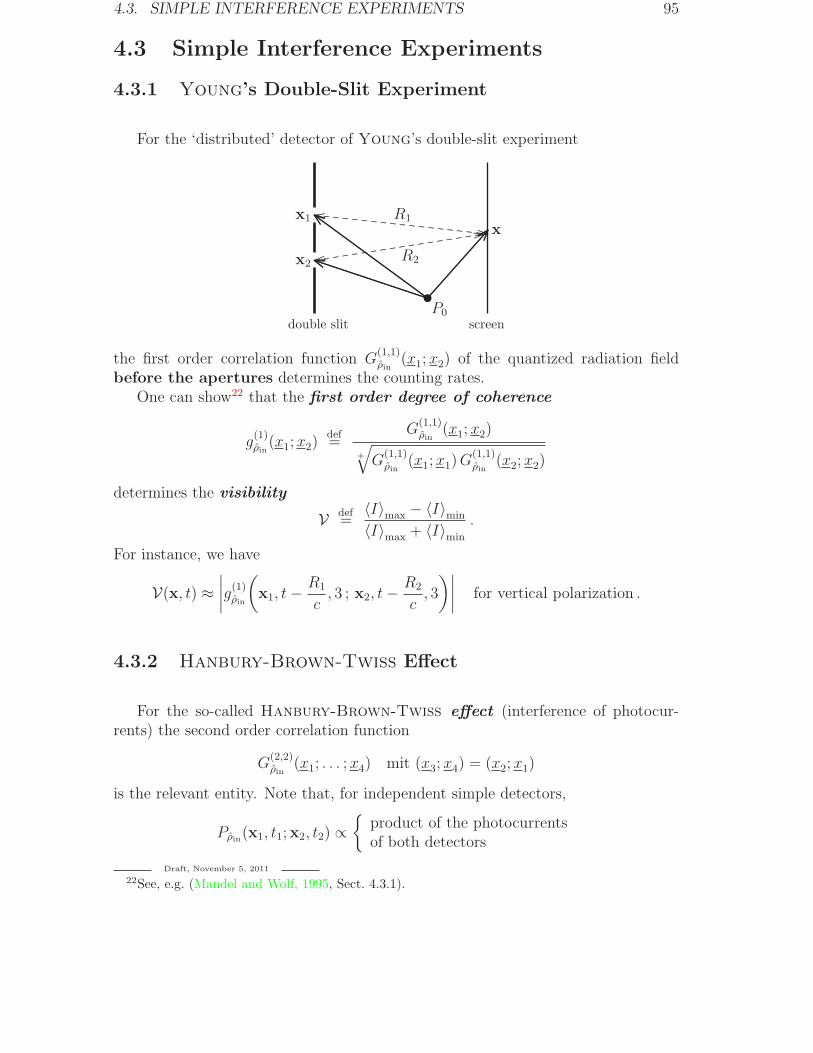
4.3. SIMPLE INTERFERENCE EXPERIMENTS 95
4.3 Simple Interference Experiments
4.3.1 Young’s Double-Slit Experiment
For the ‘distributed’ detector of Young’s double-slit experiment
uppppppppppppppppppppppppppppppppppppppppppppppppppppppppppppppppppppppppppp
ppppppppppppppppppppppppppppppppppppppppppppppppppppppppppppppppppppppppppp
ppppppppppppppppppppppppppppppppppppppppppppppppppppppppppppppppppppppppppp
pppppppppppppppppppppppppppppppppppppppppp
pppppppppppppppppppppppppppppppppppppppp
pppppppppppppppppppppppppppppppppppppppp
pppppppppppppppppppppppppppppppppppppppp
pppppppppppppppppppppppppppppppppppppppp
pppppppppppppppppppppppppppppppppppppppp
pppppppppppppppppppppppppppppppppppppppp
ppppppppppppppppppppppppp pppppppppppppppppppppppppppppppppppppppppp
pppppppppppppppppppppppppppppppppppppppppppppppppppppppppppppppppppppppppppppppppppppppppppppppppppppppppppppppppppppppppppppppppppppppppppppppppppppppppppppppppppppppppppppppppppppppppppppppppppppppppppppppppppppp
.................................................. .......... .......... .......... .......... .......... .......... .......... .......... .......... .......... .......... .......... .......... .......... .......... .......... .......... ...................................
.........
.................................................. .......... .......... .......... ..........
.......... .......... .......... .......... ..........
.......... .......... .......... .......... ..........
.......... .......... ..................................................
x1
x2
x
P0
R1
R2
double slit screen
the first order correlation function G(1,1)ρin
(x1; x2) of the quantized radiation fieldbefore the apertures determines the counting rates.
One can show22 that the first order degree of coherence
g(1)ρin(x1; x2)
def=
G(1,1)ρin
(x1; x2)
+
√G
(1,1)ρin
(x1; x1)G(1,1)ρin
(x2; x2)
determines the visibility
V def=
〈I〉max − 〈I〉min
〈I〉max + 〈I〉min
.
For instance, we have
V(x, t) ≈∣∣∣∣g
(1)ρin
(x1, t−
R1
c, 3 ; x2, t−
R2
c, 3
)∣∣∣∣ for vertical polarization .
4.3.2 Hanbury-Brown-Twiss Effect
For the so-called Hanbury-Brown-Twiss effect (interference of photocur-rents) the second order correlation function
G(2,2)ρin
(x1; . . . ; x4) mit (x3; x4) = (x2; x1)
is the relevant entity. Note that, for independent simple detectors,
Pρin(x1, t1;x2, t2) ∝
product of the photocurrentsof both detectors
Draft, November 5, 2011
22See, e.g. (Mandel and Wolf, 1995, Sect. 4.3.1).
96 CHAPTER 4. PHOTODETECTION
ifηjνj
′ν
ν ∝ δjνj′ν ∀ ν ∈ 1, 2 , jν , j′ν ∈ 1, 2, 3 .Especially for coherent states of the form
χ = e−|α|2+|β|2
2 eα a†+β b†Ω
=
(e−
|α|22 eα a
†Ω
)⊗(e−
|β|22 eβ b
†Ω
)
= double light source
with a ⊥ b we have
A(+)j(x, t)χ =⟨Ω∣∣∣ A(+)j(x, t)
(α a† + β b†
)Ω⟩χ
=(A
(+)a
j(x, t) + A
(+)b
j(x, t)
)χ
where
A(+)a
j(x, t)
def=
⟨Ω∣∣∣ A(+)j(x, t)α a† Ω
⟩,
A(+)b
j(x, t)
def=
⟨Ω∣∣∣ A(+)j(x, t) β b† Ω
⟩.
If
A(+)a
j(x, t) ≈ Aja︸︷︷︸
>0
e−i(ω t−ka·x+ϕa) ,
A(+)b
j(x, t) ≈ Ajb︸︷︷︸
>0
e−i(ω t−kb·x+ϕb)
in the considered space-time region then this implies
G(2,2)ρin
(x1; x2; x2; x1) =∣∣Aj1a e−i(ω t1−ka·x1+ϕa) + Aj1b e
−i(ω t1−kb·x1+ϕb)∣∣×
×∣∣Aj2a e−i(ω t2−ka·x2+ϕa) + Aj2b e
−i(ω t2−kb·x2+ϕb)∣∣
=
(∣∣Aj1a∣∣2 +
∣∣Aj1b∣∣2 + Aj1a A
j1b
(e−i(ϕa−ϕb) e(ka−kb)·x1 + c.c.
))×
×(∣∣Aj2a
∣∣2 +∣∣Aj2b
∣∣2 + Aj2a Aj2b
(e−i(ϕa−ϕb) e(ka−kb)·x2 + c.c.
))
and hence⟨G
(2,2)ρin
(x1; x2; x2; x1)⟩
=(|Aj1a |
2+∣∣Aj1b
∣∣2)(
|Aj2a |2+∣∣Aj2b
∣∣2)
+2Aj1a Aj2a A
j1b A
j2b cos
((ka − kb) · (x1 − x2)
)
︸ ︷︷ ︸interference term!
,
where by 〈 〉 we indicate averaging over one (or both) of the angles ϕa, ϕb . Hencefor
ρ =e−|α|2−|β|2
(2π)2
∫ 2π
ϕa=0
∫ 2π
ϕb=0
∣∣∣eα ei ϕa a†+β ei ϕb b†Ω⟩⟨eα e
i ϕa a†+β ei ϕb b†Ω∣∣∣ dϕa dϕb
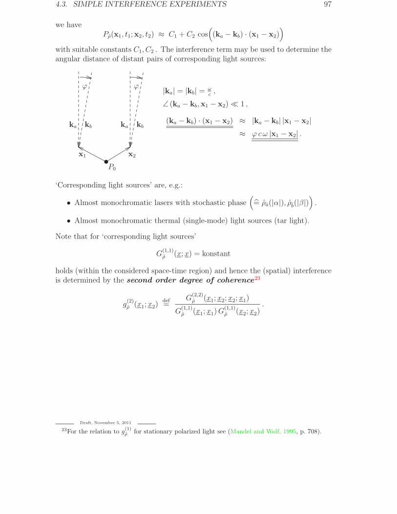
4.3. SIMPLE INTERFERENCE EXPERIMENTS 97
we havePρ(x1, t1;x2, t2) ≈ C1 + C2 cos
((ka − kb) · (x1 − x2)
)
with suitable constants C1, C2 . The interference term may be used to determine theangular distance of distant pairs of corresponding light sources:
........................................ .............................................................................
....... ............................................
u
..........
..........
..........
..........
..........
..........
..........
..........
..........
..........
..........
..........
..........
..........
..........
..........
...
........................................
..........
..........
..........
..........
..........
..........
..........
..........
..........
..........
..........
..........
..........
..........
..........
..........
...
........................................
...................................................................................................................................................................
........................................
...................................................................................................................................................................
........................................
............................
............................
............................
............................
......... ........................................
.............................................................................................................
........................................
ϕ ϕ
x2x1
ka kb ka kb
P0
|ka| = |kb| = ωc,
∠ (ka − kb,x1 − x2) ≪ 1 ,
(ka − kb) · (x1 − x2) ≈ |ka − kb| |x1 − x2|≈ ϕ cω |x1 − x2| .
‘Corresponding light sources’ are, e.g.:
• Almost monochromatic lasers with stochastic phase(= ρa(|α|), ρb(|β|)
).
• Almost monochromatic thermal (single-mode) light sources (tar light).
Note that for ‘corresponding light sources’
G(1,1)ρ (x; x) = konstant
holds (within the considered space-time region) and hence the (spatial) interferenceis determined by the second order degree of coherence23
g(2)ρ (x1; x2)
def=
G(2,2)ρ (x1; x2; x2; x1)
G(1,1)ρ (x1; x1)G
(1,1)ρ (x2; x2)
.
Draft, November 5, 2011
23For the relation to g(1)ρ for stationary polarized light see (Mandel and Wolf, 1995, p. 708).

98 CHAPTER 4. PHOTODETECTION
Chapter 5
Applications of Non-ClassicalLight
5.1 Criteria for Non-Classical Light
According to Glauber a state ρ of the radiation field is called classical if inTheorem 1.2.2 the ρN can be chosen nonnegative.1
The optical equivalence theorem explains why interference experiments with typ-ical interference pattern — as in Young’s double-slit experiment or the Hanbury-
Brown-Twiss effect — do not show any striking difference between classical andnon-classical light.
Inequalities, however, which are valid for classical light may be violated by non-classical light, since inequalities are not invariant under averaging with non-positiveweights.
For states ρFock with strictly bounded photon number this is quite obvious, sincethey fulfill the condition
G(n,n)ρFock
≡ 0 for sufficiently large n , (5.1)
whereas for classical light we always have3∑
j1,...,jn=1
∫G
(n,n)ρ (x1; . . . ; xn) dx1 · · · dxn > 0 .
Unfortunately, preparation of states with strictly bounded photon number is impos-sible and, moreover, (5.1) cannot be rigorously checked.
Better suited for experimental checks is the inequality∣∣∣G(2,2)
ρ (x1; x2; x2; x1)∣∣∣2
≤ G(2,2)ρ (x1; x1; x1; x1)G
(2,2)ρ (x2; x2; x2; x2)
for classical states ρ ∈ B(Hfield) .(5.2)
Draft, November 5, 2011
1See (Johansen, 2004) for critical remarks on Glauber’s classicality criterion. See also(Miranowicz et al., 2010).
99
100 CHAPTER 5. APPLICATIONS OF NON-CLASSICAL LIGHT
Outline of proof for (5.2): Let a1, a2, . . . be a maximal family of pairwiseorthogonal modes and define
G(n,m)α1,...,αN (x1; . . . ;xn+m)
def= Tr
(|χα1,...,αN
〉〈χα1,...,αN|(
n∏
ν=1
A(−)jν (xν , tν)
)n+m∏
µ=n−1
A(+)jµ(xµ, tµ)
).
ThenG(2,2)α1,...,αN
(x1;x2;x2;x1) = G(1,1)α1,...,αN
(x1;x1) G(1,1)α1,...,αN
(x2;x2)︸ ︷︷ ︸≥0
.
For classical states this implies
∣∣∣G(2,2)ρ (x1;x2;x2;x1)
∣∣∣2
= limN→∞
∣∣∣∣∫ρN (ξ1, . . . , ηN )︸ ︷︷ ︸
≥0
G(2,2)ξ1+i η1,...,ξN+i ηN
(x1;x2;x2;x1)dξ1 dη1π
· · · dξN dηNπ
∣∣∣∣2
= limN→∞
∣∣∣∣∫ (
+√ρN (ξ1, . . . , ηN )G
(1,1)ξ1+i η1,...,ξN+i ηN
(x1;x1))∗
×
× +√ρN (ξ1, . . . , ηN )G
(1,1)ξ1+i η1,...,ξN+i ηN
(x2;x2)dξ1 dη1π
· · · dξN dηNπ
∣∣∣∣2
≤Schwarz
limN→∞
∫ρN (ξ1, . . . , ηN )
∣∣∣G(1,1)ξ1+i η1,...,ξN+i ηN
(x1;x1)∣∣∣2
︸ ︷︷ ︸=G
(2,2)ξ1+i η1,...,ξN+i ηN
(x1;x1;x1;x1)
dξ1 dη1π
· · · dξN dηNπ
×
×∫ρN (ξ1, . . . , ηN )
∣∣∣G(1,1)ξ1+i η1,...,ξN+i ηN
(x2;x2)∣∣∣2
︸ ︷︷ ︸=G
(2,2)ξ1+i η1,...,ξN+i ηN
(x2;x2;x2;x2)
dξ1 dη1π
· · · dξN dηNπ
= G(2,2)ρ (x1;x1;x1;x1)G
(2,2)ρ (x2;x2;x2;x2) .
Definition 5.1.1 Let G = O × (τ1, τ2) be an open space-time region and let ρI bea density operator on Hfield . Then ρ
I is called stationary in G iff 2
G(n,m)
ρI(x1; . . . ; xn+m) = G
(n,m)
ρI(x1 + τ ; . . . ; xn+m + τ) ,
wherexν + τ
def= (xν , jν , tν + τ) ,
holds for all n,m ∈ N and for all x1, . . . , xn+m ∈ M and τ ∈ R with
x1, . . . , xn+m, x1 + τ, . . . , xn+m + τ ∈ G .
Remark: of course, also for stationary states there are stochastic fluc-tuations.
Draft, November 5, 2011
2It is stationary in all of space-time iff e−i~Hfield τ ρI e+
i~Hfield τ = ρI ∀ τ ∈ R .
5.1. CRITERIA FOR NON-CLASSICAL LIGHT 101
Corollary 5.1.2 Let G be as in Definition 5.1.1 and let ρ be a classical state ofthe radiation field that is stationary in G . Then
G(2,2)ρ (x; x+ τ ; x+ τ ; x) ≤ G
(2,2)ρ (x; x; x; x) (5.3)
holds for all x ∈ M and all τ ∈ R with x, x+ τ ∈ G .
Outline of proof:
(G
(2,2)ρ (x;x;x;x)︸ ︷︷ ︸=
(G
(1,1)ρ (x;x)︸ ︷︷ ︸
≥0
)2
)2=
stat.G
(2,2)ρ (x;x;x;x)G
(2,2)ρ (x+ τ ;x+ τ ;x+ τ ;x+ τ)
≥(5.2)
∣∣∣G(2,2)ρ (x;x+ τ ;x+ τ ;x)︸ ︷︷ ︸
≥0
∣∣∣2
.
While bunching
G(2,2)ρ (x; x+ τ ; x+ τ ; x) < G
(2,2)ρ (x; x; x; x) ,
is possible for stationary classical light Corollary 5.1.2 shows that anti-bunching
G(2,2)ρ (x; x+ τ ; x+ τ ; x) > G
(2,2)ρ (x; x; x; x) ,
is not possible for stationary classical light!Bunching is typical for thermal light:
If a detector fires then with high probability the intensity of the radi-ation field is considerable which — for coherent states — implies highprobability for detection of additional photons at that instant. There-fore, strong stochastic fluctuations of the momentary coherent state ofclassical radiation support bunching, i.e.:
The probability for detecting a second photon almost immedi-ately after a first one decreases with increasing time delay.
Anti-bunching is to be expected if one can arrange that single photons arrive in(essentially) fixed time intervals. This could be observed for resonance fluorescence.3
Draft, November 5, 2011
3See (Mandel and Wolf, 1995, Sect. 15.6.5) and (Kurtsiefer et al., 2000).
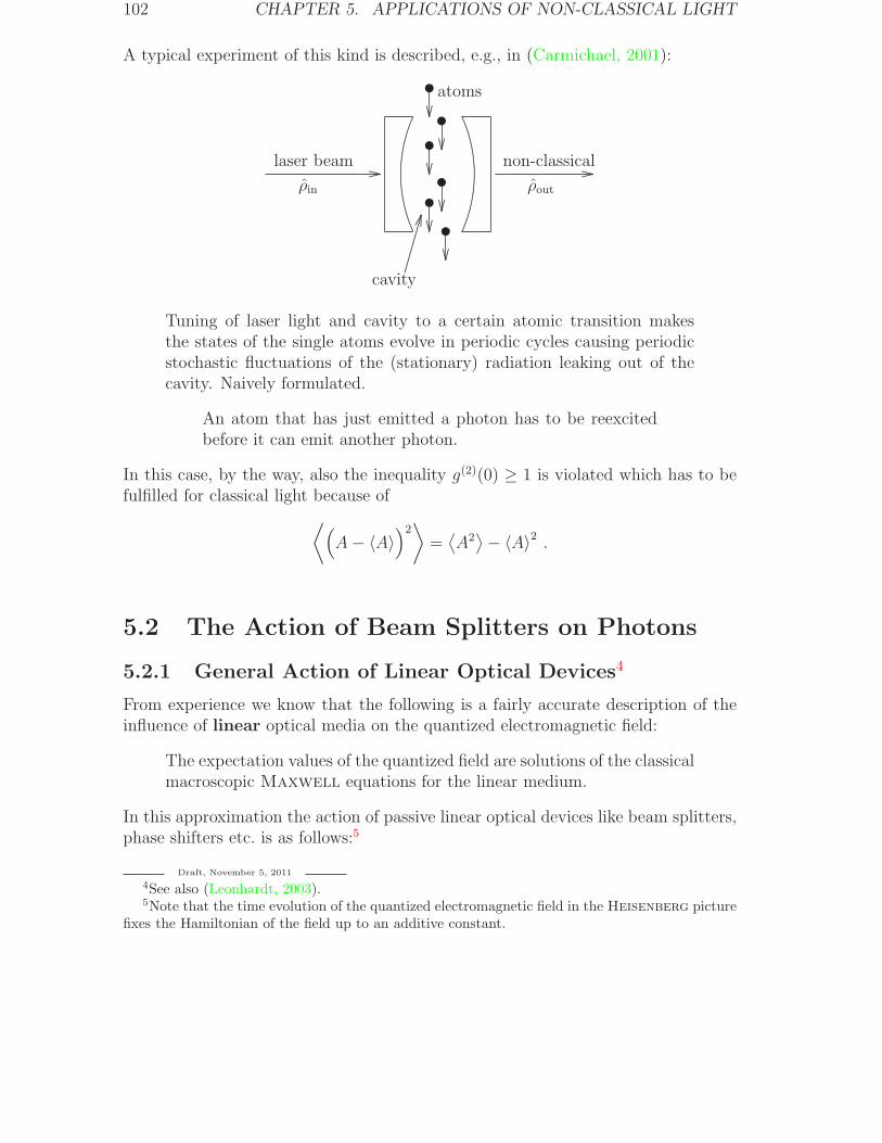
102 CHAPTER 5. APPLICATIONS OF NON-CLASSICAL LIGHT
A typical experiment of this kind is described, e.g., in (Carmichael, 2001):
u
........................................
u
........................................u
........................................
u
........................................
u
........................................
u
........................................
.............................................................................................................................................................................................................. ..............................................................................................................................................................................................................
........................................
........................................
........................................................................................................
.......
.......
..........................
atoms
laser beam
ρin ρout
non-classical
cavity
Tuning of laser light and cavity to a certain atomic transition makesthe states of the single atoms evolve in periodic cycles causing periodicstochastic fluctuations of the (stationary) radiation leaking out of thecavity. Naively formulated.
An atom that has just emitted a photon has to be reexcitedbefore it can emit another photon.
In this case, by the way, also the inequality g(2)(0) ≥ 1 is violated which has to befulfilled for classical light because of
⟨(A− 〈A〉
)2⟩=⟨A2⟩− 〈A〉2 .
5.2 The Action of Beam Splitters on Photons
5.2.1 General Action of Linear Optical Devices4
From experience we know that the following is a fairly accurate description of theinfluence of linear optical media on the quantized electromagnetic field:
The expectation values of the quantized field are solutions of the classicalmacroscopic Maxwell equations for the linear medium.
In this approximation the action of passive linear optical devices like beam splitters,phase shifters etc. is as follows:5
Draft, November 5, 2011
4See also (Leonhardt, 2003).5Note that the time evolution of the quantized electromagnetic field in the Heisenberg picture
fixes the Hamiltonian of the field up to an additive constant.
5.2. THE ACTION OF BEAM SPLITTERS ON PHOTONS 103
If aνν∈N is a maximal family of pairwise orthogonal modes and if
⟨Ω∣∣∣ A(+)(x, t) a†ν Ω
⟩7−→
⟨Ω∣∣∣ A(+)(x, t) b†ν Ω
⟩
agrees with the transformation of the complex vector potential in thecorresponding classical optics (for every ν ∈ N) then the state transfor-mation for the quantized electromagnetic field in the interaction pictureis
f(a†1, . . . , a†2, . . .) Ω 7−→ f(b†, . . . , b†2, . . .) Ω
for sufficiently well-behaved f .
For coherent states this is a direct consequence of (1.84). Therefore, according tothe optical equivalence theorem, this holds for all states of the quantized radiationfield.
5.2.2 Classical Description of Lossless Beam Splitters
Consider the action of a beam splitter , as sketched in Figure 5.1, on an incomingmonochromatic classical light beam corresponding to the complex vector potential
A(+)in (x, t) = (2π)−3/2
õ0~c
∫a in(k)e
−i(ω t−k·x) dVk√2 |k|
,
where6
a in(k) = z1in aV1(k) + z2in a
V2(k) ,
aVj(k)def=(ωc
) 32δ(k− kj) e2 ∀ j ∈ 1, 2
(5.4)
and7
k1def=ω
c
e1 − e3√2
, k2def=ω
c
e1 + e3√2
.
Linearity of the (plane) beam splitter implies that there are r1, r2, t1, t2 ∈ C suchthat the outcoming light beam corresponds to a complex vector potential
A(+)out (x, t) = (2π)−3/2
õ0~c
∫a out(k)e
−i(ω t−k·x) dVk√2 |k|
witha out(k) = z1out a
V1(k) + z2out a
V2(k)
Draft, November 5, 2011
6The zj are just complex numbers without any physical dimension.7Actually, it would be sufficient that k1 · e3 = −k2 · e3 . Then, however the action of the beam
splitter would depend on k1 · e3 , in general.
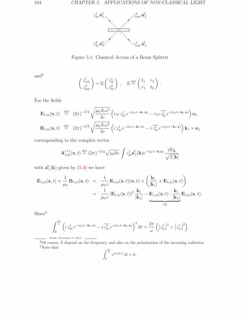
104 CHAPTER 5. APPLICATIONS OF NON-CLASSICAL LIGHT
.......... .......... .......... .......... .......... .......... .......... .......
......................................
............................
................................. .....
............................
....................
....................
....................
....................
....................
....................
.................
....................
....................
....................
....................
....................
....................
.................
z2out aV2z1in a
V1
z2in aV2 z1out a
V1
Figure 5.1: Classical Action of a Beam Splitter
and8 (z1out
z2out
)= S
(z1in
z2in
), S
def=
(t1 r2
r1 t2
).
For the fields
E1,in(x, t)def= (2π)−3/2
√µ0 ~ω2
2c
(i ω z1in e
−i(ω t−k1·x) − i ω z1in e+i(ω t−k1·x)
)e2
B1,in(x, t)def= (2π)−3/2
√µ0 ~ω2
2c
(i z1in e
−i(ω t−k1·x) − i z1in e+i(ω t−k1·x)
)k1 × e2
corresponding to the complex vector
A(+)1,in(x, t)
def= (2π)−3/2
õ0~c
∫z1ina
V1(k)e
−i(ω t−k·x) dVk√2 |k|
with aV1(k) given by (5.4) we have
E1,in(x, t)×1
µ0
B1,in(x, t) =1
µ0 cE1,in(x, t)(x, t)×
(k1
|k1|× E1,in(x, t)
)
=1
µ0 c|E1,in(x, t)|2
k1
|k1|− E1,in(x, t) ·
k1
|k1|︸ ︷︷ ︸=0
E1,in(x, t) .
Since9
∫ 2πω
0
(i z1in e
−i(ω t−k1·x) − i z1in e+i(ω t−k1·x)
)2dt =
2π
ω
(∣∣z1in∣∣2 +
∣∣z1in∣∣2)
Draft, November 5, 2011
8Of course, S depend on the frequency and also on the polarization of the incoming radiation.9Note that ∫ 2π
ω
0
e±i 2ω t dt = 0 .
5.2. THE ACTION OF BEAM SPLITTERS ON PHOTONS 105
this gives for the intensity , i.e. the modulus of the time-averaged energy currentdensity, of this stationary field
∣∣∣∣∣ω
2π
∫ 2πω
0
E0(x, t)×1
µ0
B0(x, t) dt
∣∣∣∣∣ = (2π)−3 ~ω4
2 c2
(∣∣z1in∣∣2 +
∣∣z1in∣∣2).
Since similar results hold for the fields in the other arms of the interferometer, for alossless beam splitter the condition
∣∣z1in∣∣2 +
∣∣z2in∣∣ =
∣∣z1out∣∣2 +
∣∣z2out∣∣
has to be fulfilled. This means that S has to be unitary, hence of the form
S =
(ζ1 −ζ2 eiψζ2 ζ1 eiψ
), ψ ∈ R , ζ1, ζ2 ∈ C ,
∣∣ζ1∣∣2 +
∣∣ζ2∣∣2 = 1 .
The latter may also be written in the form
S = ei ϕ(a −bb a
)φ ∈ R , a, b ∈ C , |a|2 + |b|2 = 1 (5.5)
(with ϕ = ψ/2 , a = ζ1 e−iψ/2 , and b = ζ2 e−iψ/2) or
S = ei ϕ(a b
b −a
)φ ∈ R , a, b ∈ C , |a|2 + |b|2 = 1
(with ϕ = (ψ + π) /2 + π , a = ζ1 e−i(ψ+π)/2 , and b = ζ2 e−i(ψ+π)/2). Anyway, thetransmittivity T resp. the reflectivity R is the same for both incoming rays:
R = |r1|2 = |r2|2 , T = |t1|2 = |t2|2 , R + T = 1 .
Beam splitters with R = T are called 50/50-beam splitters. Beam splitters withr1 = r2 and t1 = t2 are called symmetric. Thus:
S =eiϕ√2
(1 ∓i∓i 1
)for symmetric 50/50 beam splitters (5.6)
(see Exercise E34c) of (Lucke, eine)).
5.2.3 Transformation of Photon Modes
Let us describe the effect of beam splitters on photons as a scattering process in theinteraction picture.10
Draft, November 5, 2011
10See also (Yurke et al., 1986).
106 CHAPTER 5. APPLICATIONS OF NON-CLASSICAL LIGHT
The photon mode corresponding to the classical mode aV1 (k) resp. aV
2 (k) is(ωc
) 32 aV(k1) resp.
(ωc
) 32 aV(k2) , where
aV(k) = a2(k) ∀k ⊥ e2 ,
for the choiceǫ2(k)
def= e2 ∀k ⊥ e2 ,
and the beam splitter acts according to11
z1in aV(k1) + z2in a
V(k2) 7−→ z1out aV(k1) + z2out a
V(k2)
=(t1 z1in + r2 z2in
)aV(k1) +
(r1 z1in + t2 z2in
)aV(k2)
for arbitrary z1in, z2in ∈ C . This is equivalent to linearity plus
(aV−(k1)
aV−(k2)
)def=
(aV(k1)
aV(k2)
)7−→
(aV+(k1)
aV+(k2)
)def=
(t1 r1
r2 t2
)
︸ ︷︷ ︸=S∗=S−1
(aV(k1)
aV(k2)
). (5.7)
Remark: The scattering matrix S0 in the interaction picture fulfills
S0 Ω = Ω
andaV+(kj) = S0 a
V−(kj) S
−10 ∀ j ∈ 1, 2 .
The scattering matrix S in theHeisenberg picture — used, e.g., in (Mandel and Wolf, 1995,Section 12.12) and (Bowmeester et al., 2002, Chapter 4) — fulfills
Ωin = S Ωout
andaVin(kj) = S aVout(kj) S
−1 ∀ j ∈ 1, 2 ,where12 (
aVin(k1)
aVin(k2)
)= S
−1
(aVout(k1)
aVout(k2)
).
See Section 2.3.1 of (Lucke, qft) for a detailed discussion of the two pictures of scat-tering theory.
Draft, November 5, 2011
11Recall (1.58) and (1.60).12Some authors mystify the fact that, e.g.,
aVout(k1) = t1 aVin(k1) + r2 a
Vin(k2)
holds even if the input situation at the lower arm of the beam splitter corresponds to the vacuum.
5.2. THE ACTION OF BEAM SPLITTERS ON PHOTONS 107
For (improper) incoming n-photon states (5.7) means that the beam splitter acts as∑
j1,...,jn∈1,2cj1,...,jn
(aV(kj1) · · · aV(kjn)
)†Ω
7−→∑
j1,...,jn∈1,2cj1,...,jn
2∑
j′1=1
Sj′1j1aV(kj′1)
†
· · ·
2∑
j′n=1
Sj′njnaV(kj′n)
†
Ω ,
(5.8)
where (S1
1 S12
S21 S2
2
)def=
(t1 r2
r1 t2
).
Obviously, the total number of photons is not changed by the beam splitter.
Let us consider, for example, the special action13
aV(k1)† aV(k2)
† Ω 7−→ 1
2
(aV(k1) + i aV(k2)
)† (i aV(k1) + aV(k2)
)†
=i
2
(aV(k1)
† aV(k1)† + aV(k2)
† aV(k2)†)Ω
of a (symmetric, 50/50-) beam splitter with
S =1√2
(1 −i
−i 1
). (5.9)
Here the incoming state is a 2-photon state with one photon definitely enteringthe beam splitter from above and the other photon definitely entering the beamsplitter from below. As if agreed upon before, the photons leave the beam splittereither both on the upper side (with probability 1
2) or both on the lower side. This
so-called Hong-Ou-Mandel effect effect is often coined 2-photon interference,14
even though the relative phase of the two photon modes is irrelevant, in this case.Needless to say, there is no classical analogue for this coalescence effect.
If the action of a beam splitter with S-matrix (5.9) does not depend on thepolarization then it transforms the (improper) Bell states
Φ±=(k1,k2)
def=
1√2
(aV(k1) a
V(k2)± aH(k1) aH(k2)
)†Ω
Φ±6=(k1,k2)
def=
1√2
(aV(k1) a
H(k2)± aH(k1) aV(k2)
)†Ω ,
(5.10)
Draft, November 5, 2011
13Recall Footnote 7. For more general input k-configurations see (Scully and Zubairy, 1999,Sect. 4.4.3), where the Heisenberg picture is used.
14See (Di Giuseppe et al., 2003) for experimental verification and (McDonald and Wang, 2003;Lim and Beige, 2005) for generalization. This effect may be exploited for measurement of the spec-tral density matrix of 1-photon states (Wasilewski et al., 2007). See also (Kim and Grice, 2003)and (Zavatta et al., 2004) for additional aspects of two-photon interference. For an extensive treat-ment of two-photon interference in beam splitters see (Wang, 2003) and references given there.
108 CHAPTER 5. APPLICATIONS OF NON-CLASSICAL LIGHT
where
aH(k) = a1(k) , ǫ2(k) = e2 ×k
|k| ∀ k︸︷︷︸6=0
⊥ e2 ,
according to
Φ±=(k1,k2) 7−→ 1
2√2
2∑
j=1
(aV(kj) a
V(kj) + aH(kj) aH(kj)
)†Ω ,
Φ+6=(k1,k2) 7−→ i√
2
2∑
j=1
(aV(kj) a
H(kj))†Ω ,
Φ−6=(k1,k2) 7−→ 1√
2
(aV(k1) a
H(k2)− aH(k1) aV(k2)
)†Ω .
Note that Φ−6= is the only Bell state that is transformed into a state with exactly
one photon leaving the beam splitter on each side.15 This effect was exploited inthe first experiment on (partial) quantum teleportation (Bowmeester et al., 1997);see also (Gisin et al., 2003).
Comment: By straightforward calculation (see 5.3.3) one can show that
χ(k1)⊗ Φ−6=(k2,k3)
=1
2
(Φ+
=(k1,k2)⊗ U1 χ(k3)− Φ+6=(k1,k2)⊗ U2 χ(k3)
+ Φ−=(k1,k2)⊗ U3 χ(k3)− Φ−
6=(k1,k2)⊗ χ(k3))
holds for
χ(k)def=(λV a
V(k) + λH aH(k)
)†Ω
and
Uj χ(k)def=
(−λH aV(k) + λV a
H(k))†
Ω for j = 1 ,(λV a
V(k)− λH aH(k)
)†Ω for j = 2 ,
(λH a
V(k) + λV aH(k)
)†Ω for j = 3 .
This allows for quantum teleportation:
Alice checks in which of the four Bell states photon 1 and 2 (corresponding to k1
and k2) are and communicates (by classical means) the result to Bob. If, e.g., Alicefound Φ+
=(k1,k2) then Bob just has to apply U−11 to photon 3 (corresponding to k3)
in order to get its polarization state equal to the unknown16 original polarizationstate of photon 1.
Of great practical use are also polarizing beam splitters, transmitting thehorizontal modes and reflecting the vertical modes. Appropriately oriented, these
Draft, November 5, 2011
15See also (Pittman and Franson, 2003) in this connection.16See (Caves et al., 2002) concerning the notion of unknown state in quantum mechanics.
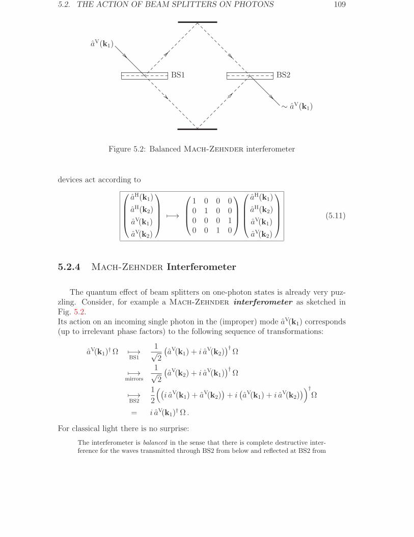
5.2. THE ACTION OF BEAM SPLITTERS ON PHOTONS 109
.......... .......... .......... .......... .......... .......... .......... .......... .......... .........
................................................
..................................
.........................................
....................
....................
....................
....................
....................
....................
....................
...............
.......... .......... .......... .......... .......... .......... .......... .......... .......... .........
.........................................
......................................... .......
..................................
....................
....................
....................
....................
....................
....................
....................
...............
....................
....................
....................
....................
....................
....................
....................
................ ..........
....................
....................
....................
....................
....................
....................
....................
.....
..................
..................
..................
..................
..................
..................
..................
..................
............
............................................................................................................................................................
aV(k1)
∼ aV(k1)
BS1 BS2
Figure 5.2: Balanced Mach-Zehnder interferometer
devices act according to
aH(k1)
aH(k2)
aV(k1)
aV(k2)
7−→
1 0 0 00 1 0 00 0 0 10 0 1 0
aH(k1)
aH(k2)
aV(k1)
aV(k2)
(5.11)
5.2.4 Mach-Zehnder Interferometer
The quantum effect of beam splitters on one-photon states is already very puz-zling. Consider, for example a Mach-Zehnder interferometer as sketched inFig. 5.2.Its action on an incoming single photon in the (improper) mode aV(k1) corresponds(up to irrelevant phase factors) to the following sequence of transformations:
aV(k1)†Ω 7−→
BS1
1√2
(aV(k1) + i aV(k2)
)†Ω
7−→mirrors
1√2
(aV(k2) + i aV(k1)
)†Ω
7−→BS2
1
2
((i aV(k1) + aV(k2)
)+ i(aV(k1) + i aV(k2)
))†Ω
= i aV(k1)† Ω .
For classical light there is no surprise:
The interferometer is balanced in the sense that there is complete destructive inter-ference for the waves transmitted through BS2 from below and reflected at BS2 from
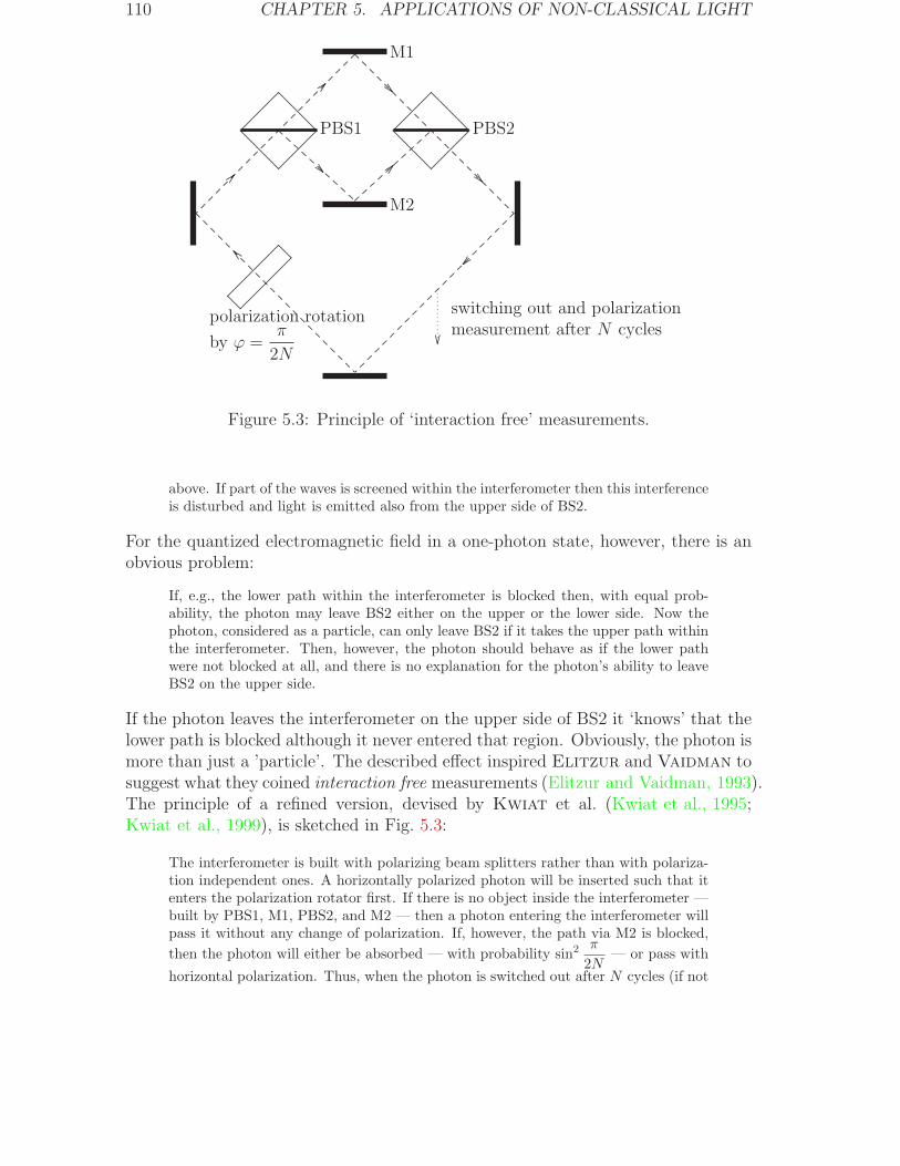
110 CHAPTER 5. APPLICATIONS OF NON-CLASSICAL LIGHT
.......................................................................................................................................................................................................................................................................................................
..................
..................
..................
..................
..........................................................................................................................................................................................................................................................................................................
..................
..................
..................
..................
...
....................
....................
....................
....................
....................
....................
....................
....................
....................
....................
..............
....................
....................
....................
....................
....................
....................
....................
....................
....................
....................
..............
....................
....................
....................
....................
....................
....................
....................
....................
....................
....................
..............
.......... .......... .......... .......... .......... .......... .......... .......... .......... ..............................
....................
....................
....................
....................
....................
....................
....................
....................
....................
....................
....................
....................
....................
....................
..............
.................................... ......
..............................
.................................... ......
..............................
..........................................
..............................
...... .............................. ......
..............................
.
.
.
.
.
.
.
.
.
.
.
.
.
...............................
..............................................................................................................................................................................................................................................................................................
..................
....
PBS2PBS1
M1
M2
switching out and polarizationmeasurement after N cycles
polarization rotation
by ϕ =π
2N
Figure 5.3: Principle of ‘interaction free’ measurements.
above. If part of the waves is screened within the interferometer then this interferenceis disturbed and light is emitted also from the upper side of BS2.
For the quantized electromagnetic field in a one-photon state, however, there is anobvious problem:
If, e.g., the lower path within the interferometer is blocked then, with equal prob-ability, the photon may leave BS2 either on the upper or the lower side. Now thephoton, considered as a particle, can only leave BS2 if it takes the upper path withinthe interferometer. Then, however, the photon should behave as if the lower pathwere not blocked at all, and there is no explanation for the photon’s ability to leaveBS2 on the upper side.
If the photon leaves the interferometer on the upper side of BS2 it ‘knows’ that thelower path is blocked although it never entered that region. Obviously, the photon ismore than just a ’particle’. The described effect inspired Elitzur and Vaidman tosuggest what they coined interaction free measurements (Elitzur and Vaidman, 1993).The principle of a refined version, devised by Kwiat et al. (Kwiat et al., 1995;Kwiat et al., 1999), is sketched in Fig. 5.3:
The interferometer is built with polarizing beam splitters rather than with polariza-tion independent ones. A horizontally polarized photon will be inserted such that itenters the polarization rotator first. If there is no object inside the interferometer —built by PBS1, M1, PBS2, and M2 — then a photon entering the interferometer willpass it without any change of polarization. If, however, the path via M2 is blocked,
then the photon will either be absorbed — with probability sin2π
2N— or pass with
horizontal polarization. Thus, when the photon is switched out after N cycles (if not
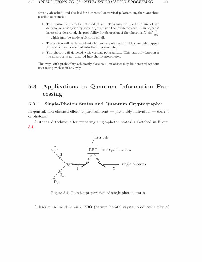
5.3. APPLICATIONS TO QUANTUM INFORMATION PROCESSING 111
already absorbed) and checked for horizontal or vertical polarization, there are threepossible outcomes:
1. The photon will not be detected at all. This may be due to failure of thedetector or absorption by some object inside the interferometer. If an object is
inserted as described, the probability for absorption of the photon is N sin2π
2N— which may be made arbitrarily small.
2. The photon will be detected with horizontal polarization. This can only happenif the absorber is inserted into the interferometer.
3. The photon will detected with vertical polarization. This can only happen ifthe absorber is not inserted into the interferometer.
This way, with probability arbitrarily close to 1, an object may be detected withoutinteracting with it in any way.
5.3 Applications to Quantum Information Pro-
cessing
5.3.1 Single-Photon States and Quantum Cryptography
In general, non-classical effect require sufficient — preferably individual — controlof photons.
A standard technique for preparing single-photon states is sketched in Figure5.4.
.......................................
...........
.................................................
....................
....................
....................
..........
....................
....................
....................
..........
..........
......................................................
..........
..........................
............................
.............................................................................................................................................................
qqqqqqqqqqqqqqqqqqqqqqqqqqqqqqqqqqqqqqqqqqqqqqqqqqqqqqqqqqqqqqqqqqqqq
.......................................................................................................
qqqqqqqqqqqqqqqqqqqqqqqqqqqqqqqqqqqqqqqqqqqqqqqqqqqqqqqqqqqqqqqqqqqqq..........................
............................
......................................................
..........
...................................................... ..........
......................................................
single photons
D2
D1
J
J⊥
BSP1 2
BBO
laser puls
“EPR pair” creation
Figure 5.4: Possible preparation of single-photon states.
A laser pulse incident on a BBO (barium borate) crystal produces a pair of
112 CHAPTER 5. APPLICATIONS OF NON-CLASSICAL LIGHT
photon with polarization state
Ψ−def=
1√2
(V︸︷︷︸
=
(10
)⊗ H︸︷︷︸
=
(01
)−H⊗V
)
via spontaneous down conversion17 and this internal state fulfills the condition
J ∈ C3
‖J‖ = 1
=⇒ Ψ− =
1√2(J⊗ J⊥ − J⊥ ⊗ J) ,
where: (ab
)
⊥
def=
(+b∗
−a∗)
∀ a, b ∈ C .
From this we conclude:
• The internal quantum state of the ensemble of those photonsrunning to the right and having a partner making detector D2 fireafter passing a J-J⊥ beam splitter has to be described (accordingto quantum mechanics) by the density operator ρ = |J〉〈J|.
• The internal quantum state of the ensemble of all photons run-ning to the right — irrespective of the behavior of their partners —corresponds to
ρ =1
21 =
1
2|J〉〈J|+ 1
2|J⊥〉〈J⊥| .
The result of a J-J⊥ test (“which detector fires?”) on photon 1 (left running)predetermines the result of an eventually following J-J⊥ test on photon 2 (runningto the right):
J⊥ for photon 1 =⇒ J for photon 1
J for photon 1 =⇒ J⊥ for photon 1
(strict correlations).If it were possible to produce exact copies of the unknown state of photon 2,
owned by Bob (far away from Alice ), then Bob could produce an ensemble ofphotons with internal state J resp. J⊥ if photon 1, owned by Alice, just passed aJ-J⊥ beam splitter and made detector 2 resp. 1 fire. Since the states of (sufficientlylarge) ensembles can be determined (quantum state tomography) Bob could imme-diately check Alice’s choice of J-J⊥ alternative. This could be exploited by Alicefor superluminal communication of information to Bob encoded in different choicesof J-J⊥ alternatives.18
Conclusion:
Draft, November 5, 2011
17See, e.g., (Gatti et al., 2003) for details.18See(Herbert, 1982) in this connection.
5.3. APPLICATIONS TO QUANTUM INFORMATION PROCESSING 113
The principles of special relativity exclude the possibility of producingexact copies of unknown quantum states (no cloning theorem).
The reason:
Every attempt to gain information not available a priori about a quantum systemusually results in uncontrollable changes of the system’s state.
The no cloning theorem opens up the possibility of single-photon quantum crypto-graphy:
If Alice and Bob both are provided with some random N -bit sequence
k = (k1, . . . , kN )
known only to them they can use this for encryption19
b = (b1, . . . , bN) 7−→ b⊕ kdef= (b1 ⊕ k1, . . . , bN ⊕ kN)
of any N -bit information b . Alice can send the N -bit sequence b+k through somepublic channel to Bob without being afraid that any eavesdropper could make useof this. Bob however can decrypt the message according to
b⊕ k 7−→ (b⊕ k)⊕ k = b
(thanks to k⊕ k = (0, . . . , 0)). Thus:
The essential point for secure secret information exchange is the abilityof Alice and Bob to create a common random key k known only to them.
A well established20 technology for secret key distribution is based on the so-called BB84 protocol suggested by (Bennet and Brassard, 1984):
Alice and Bob agree upon two alternatives J-J⊥ and J′-J′⊥ with
|〈J | J′〉|2 = 1
2.
Moreover they agree on certain instants of time at which Alice will send a photonto Bob with internal state being randomly chosen from the set J,J⊥,J′,J′
⊥ . Bobrandomly chooses a test of either the J-J⊥ or the J′-J′
⊥ alternative for the received
Draft, November 5, 2011
19As usual, ⊕ means modulo-2 addition:
b⊕ kdef= (b+ k) mod 2 ∀ b, k ∈ 0, 1 .
20See http://www.idquantique.com. For more recent implementations of quantum key distri-bution see (Sasaki et al., 2011) and references given there.
114 CHAPTER 5. APPLICATIONS OF NON-CLASSICAL LIGHT
photon. After all photons are sent and tested Alice and Bub determine, via publiccommunication, those instances for which by chance the had chosen the same al-ternative. For these instances their results are strictly correlated (in the ideal case)— unless the sending war perturbed (by an eavesdropper, for example). If thesecorrelations are confirmed for certain randomly chosen instance then the other Nresults, kept secret, provide the common key.
The crucial point, however, is to make sure that (essentially) only sin-gle photons are sent21 in order to prohibit — thanks to the no cloningtheorem — eavesdropping.
5.3.2 Entangled Pairs of Photons
Figure 5.4 also serves as a good illustration of the following well-known considerationby Einstein, Rosen, and Podolsky (EPR):
1. According to EPR the result of any test of a J,J⊥ alternative for photon 2should be predetermined (determinism) since: Without influencing photon 2in any way (locality) one could test the J,J⊥ alternative on photon 1 and usethe result to predict — thanks to the strict correlation of the photons — theoutcome of a corresponding subsequent test on photon 2 with certainty.
2. From this point of view quantum mechanics appears to be incomplete (exis-tence of hidden variables) since there is no quantum mechanical state predict-ing for all J-J⊥ alternatives the outcome of a corresponding test with certainty.
This should be confronted with another well-know consideration by Bell which —in a slightly modified form — is as follows:
Let Φ be a (large but finite) ensemble of photon pairs in the state Ψ− . Then,according to EPR the definition
ΦJ,J′def=
pairs from Φ with:
J predeterminded for photon 1 andJ′ predetermined for photon 2
should be allowed (determinism) for every ensemble of EPR pairs (photons 1 and2) and
ΦJdef= ΦJ,J′ ∪ ΦJ,J′
⊥
should be independent of J′ (locality). The correlations of the EPR pairs then imply
ΦJ,J′ = ΦJ ∩ ΦJ′ ∀J,J′ (5.12)
Draft, November 5, 2011
21See (Alleaume et al., 2003) and references given there for realizations of single-photon sources.
5.3. APPLICATIONS TO QUANTUM INFORMATION PROCESSING 115
and, consequently, for all Jones vectors J2,J2,J3 the inequality22
|ΦJ1,J2 | ≤ |ΦJ1,J3 |+ |ΦJ2,J3⊥ | (5.13)
has to be fulfilled.
Outline of proof: The inequality follows from
χ1 χ2 ≤ χ1 χ3 + χ2 (1− χ3) ∀χ1, χ2, χ3 ∈ 0, 1 ,
since23
|ΦJν| =
∑
x∈ΦJν
χΦJν(x) , |ΦJν⊥
| =∑
x∈ΦJν
(1− χΦJν
(x))
andχΦJν∩ΦJµ
(x) = χΦJν(x)χΦJµ
(x) .
Therefore (5.12) contradicts the quantum mechanical predictions
|ΦJ| / |Φ| =1
2,
|ΦJ′,J⊥ | / |Φ| =1
2|〈J | J′〉|2
∀J,J′ . (5.14)
This is because for, e.g.,
Jνdef=
(cos(ν π8
)
sin(ν π6
))
∀ ν ∈ 1, 2, 3
(5.14) implies
|ΦJ1,J2 ||Φ| =
1
2cos2 (π/6)
= 3/8
≥ 2/8
=1
2cos2(π/3) +
1
2
(1− cos2(π/6)
)
=|ΦJ1,J3 |+ |ΦJ2,J3⊥ |
|Φ|
rather than (5.13). Naive proposal:
Draft, November 5, 2011
22By |Φν | we denote the number of elements of the set Φν .23As usual we denote by χΦ′ the characteristic function of the set Φ′ :
χΦ′(x)def=1 for x ∈ Φ′ ,0 sonst .
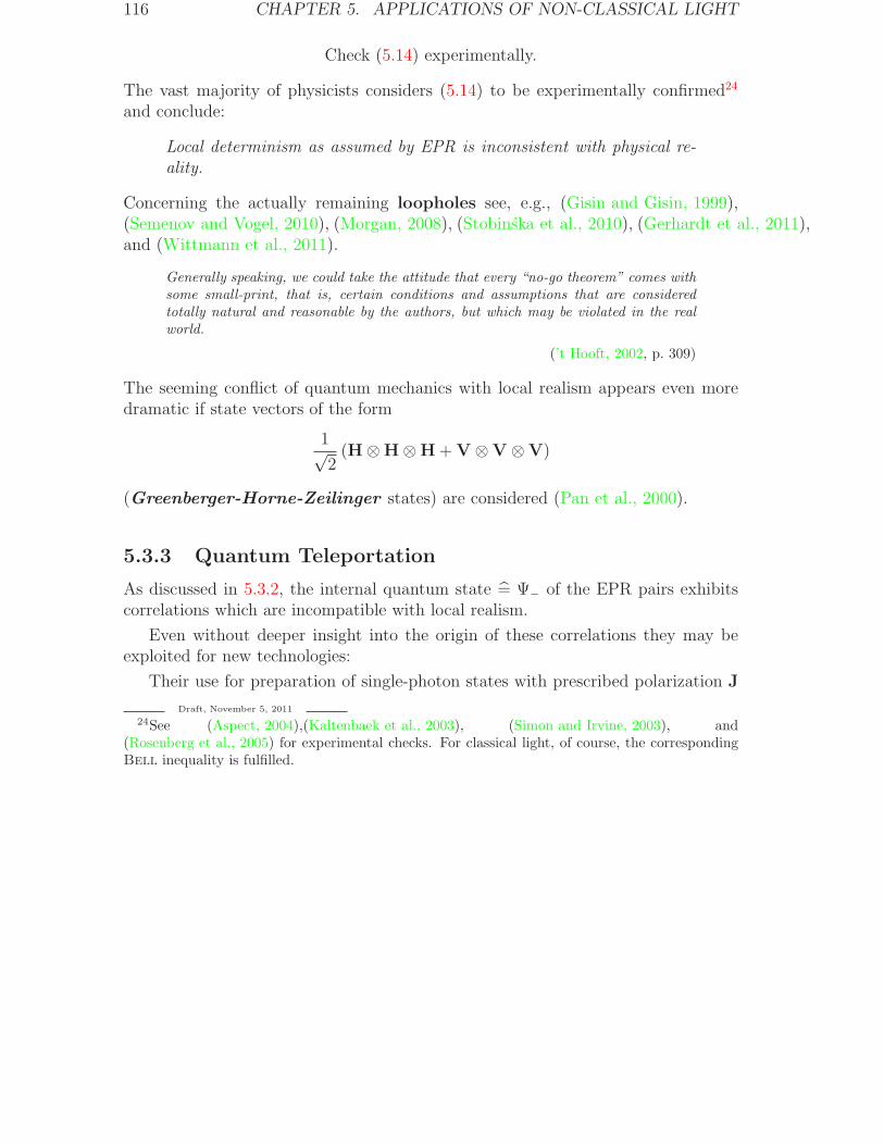
116 CHAPTER 5. APPLICATIONS OF NON-CLASSICAL LIGHT
Check (5.14) experimentally.
The vast majority of physicists considers (5.14) to be experimentally confirmed24
and conclude:
Local determinism as assumed by EPR is inconsistent with physical re-ality.
Concerning the actually remaining loopholes see, e.g., (Gisin and Gisin, 1999),(Semenov and Vogel, 2010), (Morgan, 2008), (Stobinska et al., 2010), (Gerhardt et al., 2011),and (Wittmann et al., 2011).
Generally speaking, we could take the attitude that every “no-go theorem” comes withsome small-print, that is, certain conditions and assumptions that are consideredtotally natural and reasonable by the authors, but which may be violated in the realworld.
(’t Hooft, 2002, p. 309)
The seeming conflict of quantum mechanics with local realism appears even moredramatic if state vectors of the form
1√2(H⊗H⊗H+V ⊗V ⊗V)
(Greenberger-Horne-Zeilinger states) are considered (Pan et al., 2000).
5.3.3 Quantum Teleportation
As discussed in 5.3.2, the internal quantum state = Ψ− of the EPR pairs exhibitscorrelations which are incompatible with local realism.
Even without deeper insight into the origin of these correlations they may beexploited for new technologies:
Their use for preparation of single-photon states with prescribed polarization J
Draft, November 5, 2011
24See (Aspect, 2004),(Kaltenbaek et al., 2003), (Simon and Irvine, 2003), and(Rosenberg et al., 2005) for experimental checks. For classical light, of course, the correspondingBell inequality is fulfilled.
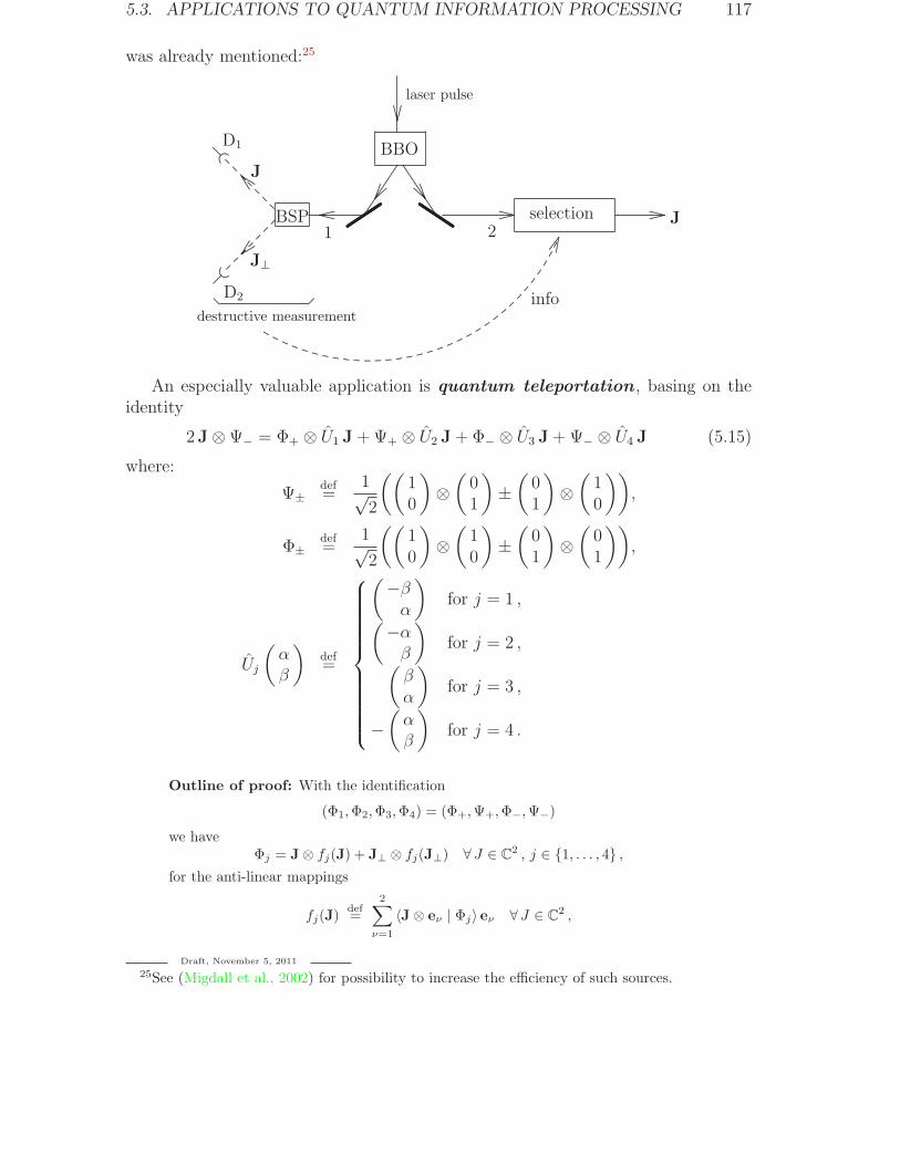
5.3. APPLICATIONS TO QUANTUM INFORMATION PROCESSING 117
was already mentioned:25
.......................................
...........
.................................................
.......
.......
.......
.................................
.......... .......... .......... .......... .......... .......... .......... .......... .......... .......... .......... .......... .......... .......... .......... ..........
.......... .......... ...
....... ..........
....................
....................
....................
.......................................................................
....................
....................
....................
..........
....................
....................
....................
..........
..........
......................................................
..........
..........................
............................
.............................................................................................................................................................
qqqqqqqqqqqqqqqqqqqqqqqqqqqqqqqqqqqqqqqqqqqqqqqqqqqqqqqqqqqqqqqqqqqqq
.......................................................................................................
qqqqqqqqqqqqqqqqqqqqqqqqqqqqqqqqqqqqqqqqqqqqqqqqqqqqqqqqqqqqqqqqqqqqq..........................
............................
......................................................
..........
...................................................... ..........
......................................................
.............. ..............
.....................................................
.
D2
D1
J
J⊥
BSP1 2
BBO
laser pulse
destructive measurementinfo
selection J
An especially valuable application is quantum teleportation , basing on theidentity
2J⊗Ψ− = Φ+ ⊗ U1 J+Ψ+ ⊗ U2 J+ Φ− ⊗ U3 J+Ψ− ⊗ U4 J (5.15)
where:
Ψ±def=
1√2
((10
)⊗(01
)±(01
)⊗(10
)),
Φ±def=
1√2
((10
)⊗(10
)±(01
)⊗(01
)),
Uj
(αβ
)def=
(−βα
)for j = 1 ,
(−αβ
)for j = 2 ,
(βα
)for j = 3 ,
−(αβ
)for j = 4 .
Outline of proof: With the identification
(Φ1,Φ2,Φ3,Φ4) = (Φ+,Ψ+,Φ−,Ψ−)
we haveΦj = J⊗ fj(J) + J⊥ ⊗ fj(J⊥) ∀ J ∈ C
2 , j ∈ 1, . . . , 4 ,for the anti-linear mappings
fj(J)def=
2∑
ν=1
〈J⊗ eν | Φj〉 eν ∀ J ∈ C2 ,
Draft, November 5, 2011
25See (Migdall et al., 2002) for possibility to increase the efficiency of such sources.
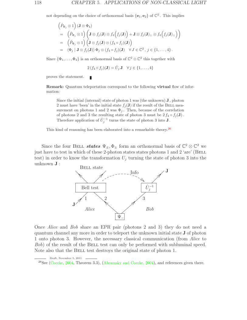
118 CHAPTER 5. APPLICATIONS OF NON-CLASSICAL LIGHT
not depending on the choice of orthonormal basis e1, e2 of C2 . This implies
(PΦj
⊗ 1)(J⊗ Φ4)
=(PΦj
⊗ 1)(
J⊗ fj(J)⊗ f4
(fj(J)
)+ J⊗ fj(J)⊥ ⊗ f4
(fj(J)⊥
))
=(PΦj
⊗ 1)(
J⊗ fj(J)⊗ (f4 fj)(J))
= 〈Φj | J⊗ fj(J)〉Φj ⊗ (f4 fj)(J) ∀ J ∈ C2 , j ∈ 1, . . . , 4 .
Since Φ1, . . . ,Φ4 is an orthonormal basis of C2 ⊗ C2 this together with
2 (f4 fj)(J) = Uj J ∀ j ∈ 1, . . . , 4
proves the statement.
Remark: Quantum teleportation correspond to the following virtual flow of infor-mation:
Since the initial (internal) state of photon 1 was (the unknown) J , photon2 must have ‘been’ in the initial state fj(J) if the result of the Bell mea-surement on photons 1 and 2 was Φj . Then, because of the correlationof photons 2 and 3 the resulting state of photon 3 must be 2 f4 fj(J) .Therefore application of U−1
j turns the state of photon 3 into J .
This kind of reasoning has been elaborated into a remarkable theory.26
Since the four Bell states Ψ±,Φ± form an orthonormal basis of C2 ⊗ C2 we
just have to test in which of these 2-photon states states photons 1 and 2 ‘are’ (Bell
test) in order to know the transformation Uj turning the state of photon 3 into theunknown J :
......................................................
....................
....................
........................................................................................................................
............................................................................................................
............................................................................................................
............................................................................................................
..........................................................................................................................................................................................................
..........................................................................................................................................................................................................
............................................................................................................
..........
......................................................
..........
......................................................
..........
......................................................
..........
......................................................
..........
..........................
............................
..........
..........................
............................
Bell stateJ
U−1j
Ψ−
Bell test
Alice Bob
Info
J
2 31
Once Alice and Bob share an EPR pair (photons 2 and 3) they do not need aquantum channel any more in order to teleport the unknown initial state J of photon1 onto photon 3. However, the necessary classical communication (from Alice toBob) of the result of the Bell test can only be performed with subluminal speed.Note also that the Bell test destroys the original state of photon 1.
Draft, November 5, 2011
26See (Coecke, 2004, Theorem 3.3), (Abramsky and Coecke, 2004), and references given there.
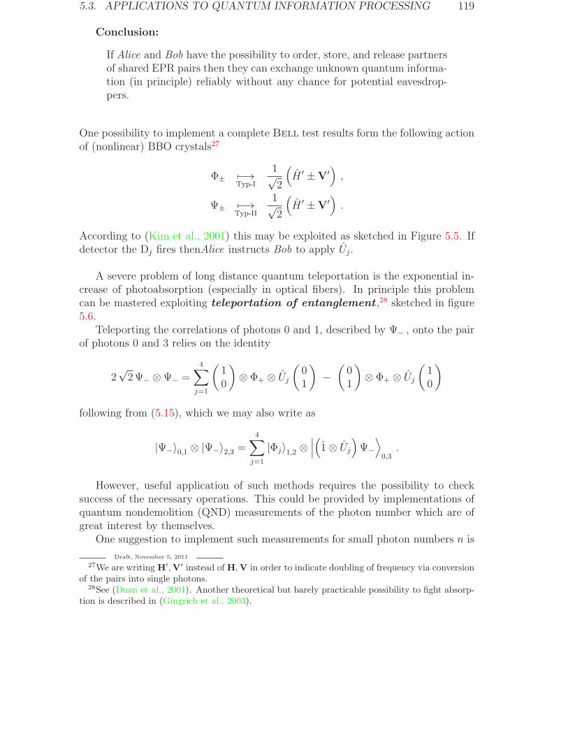
5.3. APPLICATIONS TO QUANTUM INFORMATION PROCESSING 119
Conclusion:
If Alice and Bob have the possibility to order, store, and release partnersof shared EPR pairs then they can exchange unknown quantum informa-tion (in principle) reliably without any chance for potential eavesdrop-pers.
One possibility to implement a complete Bell test results form the following actionof (nonlinear) BBO crystals27
Φ± 7−→Typ-I
1√2
(H ′ ±V′
),
Ψ± 7−→Typ-II
1√2
(H ′ ±V′
).
According to (Kim et al., 2001) this may be exploited as sketched in Figure 5.5. Ifdetector the Dj fires thenAlice instructs Bob to apply Uj.
A severe problem of long distance quantum teleportation is the exponential in-crease of photoabsorption (especially in optical fibers). In principle this problemcan be mastered exploiting teleportation of entanglement ,28 sketched in figure5.6.
Teleporting the correlations of photons 0 and 1, described by Ψ− , onto the pairof photons 0 and 3 relies on the identity
2√2Ψ− ⊗Ψ− =
4∑
j=1
(10
)⊗ Φ+ ⊗ Uj
(01
)−(01
)⊗ Φ+ ⊗ Uj
(10
)
following from (5.15), which we may also write as
|Ψ−〉0,1 ⊗ |Ψ−〉2,3 =4∑
j=1
|Φj〉1,2 ⊗∣∣∣(1⊗ Uj
)Ψ−⟩0,3
.
However, useful application of such methods requires the possibility to checksuccess of the necessary operations. This could be provided by implementations ofquantum nondemolition (QND) measurements of the photon number which are ofgreat interest by themselves.
One suggestion to implement such measurements for small photon numbers n is
Draft, November 5, 2011
27We are writing H′,V′ instead of H,V in order to indicate doubling of frequency via conversionof the pairs into single photons.
28See (Duan et al., 2001). Another theoretical but barely practicable possibility to fight absorp-tion is described in (Gingrich et al., 2003).
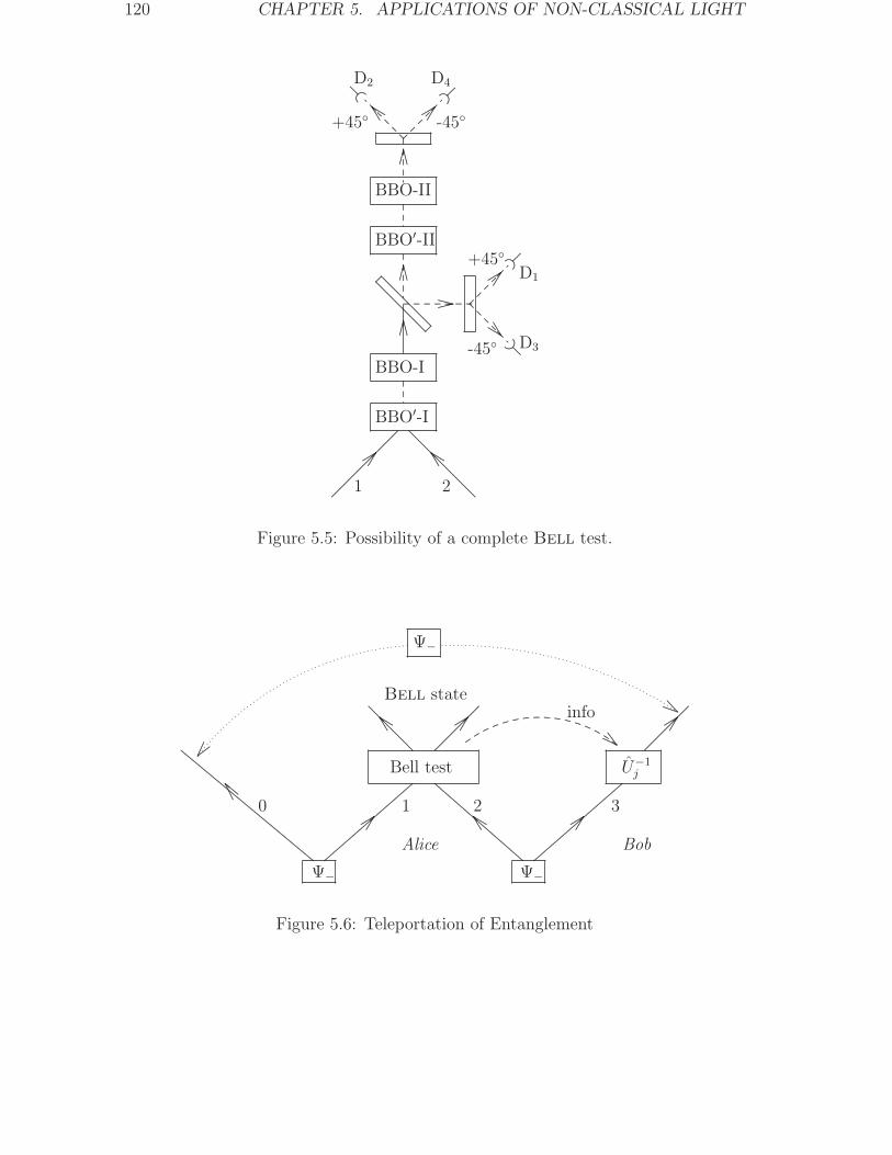
120 CHAPTER 5. APPLICATIONS OF NON-CLASSICAL LIGHT
............................................
..................
....................
....................
..............
..........
......................................................
......................................................
..................................................
............................... ...................
........................................
..........
............................... ...................
..........
..........
..
....................................................
..........
..........
..........
..........
....
......................................................
..........
..........
..........
..........
....
..........
..........................
............................
..........
..........
..........
..........
..........
....
..........
....................................................
......................................................
.........................................................................................................................
.........................................................................................................................
..............
..............
.......... .......... .......... .......... .......... .......... ..........
......................................................
.....................................................
.
..........
..........
..
.................................................................................................................................................................
..................................................................................................................................................................
..........
......................................................
..........
..........................
............................
1 2
BBO′-I
BBO-I
BBO′-II
BBO-II
+45 -45
+45
-45 D3
D1
D2 D4
Figure 5.5: Possibility of a complete Bell test.
......................................................
....................
....................
..............................................................................................................................................................
................
..............................................................
......................................................
....
....
.....
......
......
.......
.........
.......................
............................................................................................................
............................................................................................................
..........................................................................................................................................................................................................
..........................................................................................................................................................................................................
............................................................................................................
..........
......................................................
..........
......................................................
..........
......................................................
..........
..........................
............................
..........
..........................
............................
..........................................................................................................................................................................................................
..........
......................................................
....................
....................
....................
....................
....................
....................
....................
....................
....................
....................
....................
....................
....................
....................
.................
..........
....................
........................................
Bell state
U−1j
Ψ−
Bell test
Alice Bob
info
2 310
Ψ−
Ψ−
Figure 5.6: Teleportation of Entanglement
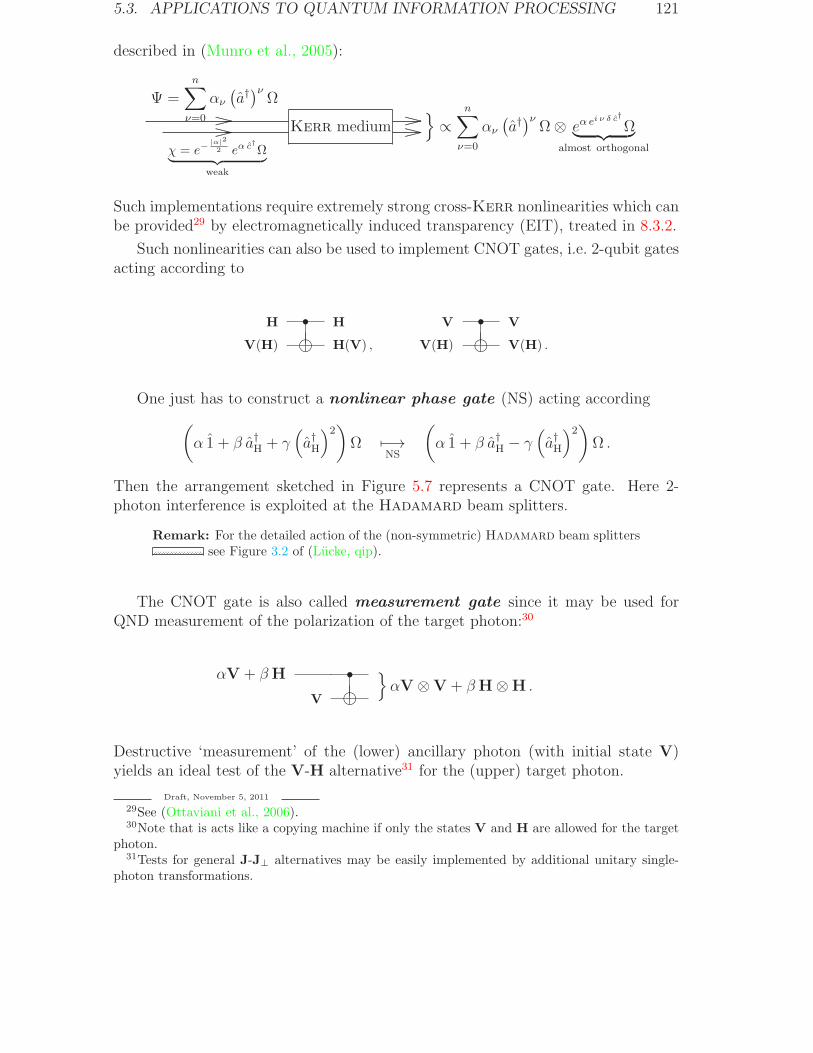
5.3. APPLICATIONS TO QUANTUM INFORMATION PROCESSING 121
described in (Munro et al., 2005):
....................................................
........
....................................................
.................................
...................................
....................................................
........
Ψ =n∑
ν=0
αν(a†)ν
Ω
χ = e−|α|2
2 eα c†
Ω︸ ︷︷ ︸weak
Kerr medium∝
n∑
ν=0
αν(a†)ν
Ω⊗ eα ei ν δ c†
Ω︸ ︷︷ ︸almost orthogonal
Such implementations require extremely strong cross-Kerr nonlinearities which canbe provided29 by electromagnetically induced transparency (EIT), treated in 8.3.2.
Such nonlinearities can also be used to implement CNOT gates, i.e. 2-qubit gatesacting according to
H s H
V(H) h H(V) ,
V s V
V(H) h V(H) .
One just has to construct a nonlinear phase gate (NS) acting according
(α 1 + β a†H + γ
(a†H
)2)Ω 7−→
NS
(α 1 + β a†H − γ
(a†H
)2)Ω .
Then the arrangement sketched in Figure 5.7 represents a CNOT gate. Here 2-photon interference is exploited at the Hadamard beam splitters.
Remark: For the detailed action of the (non-symmetric) Hadamard beam splitters..................................... see Figure 3.2 of (Lucke, qip).
The CNOT gate is also called measurement gate since it may be used forQND measurement of the polarization of the target photon:30
αV + βH s
V h
αV ⊗V + βH⊗H .
Destructive ‘measurement’ of the (lower) ancillary photon (with initial state V)yields an ideal test of the V-H alternative31 for the (upper) target photon.
Draft, November 5, 2011
29See (Ottaviani et al., 2006).30Note that is acts like a copying machine if only the states V and H are allowed for the target
photon.31Tests for general J-J⊥ alternatives may be easily implemented by additional unitary single-
photon transformations.
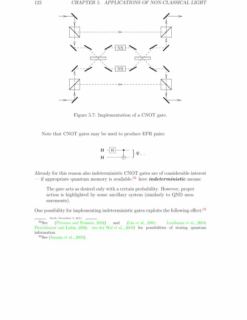
122 CHAPTER 5. APPLICATIONS OF NON-CLASSICAL LIGHT
......................................................... .......................................................
pppppppppppppppppppppppppppppppppppppppppppppppppppppppppppppppppppppppppppppppppppppppppppp
pppppppppppppppppppppppppppppppppppppppppppppppppppppppppppppppppppppppppppppppppppppppppppp
pppppppppppppppppppppppppppppppppppppppppppppppppppppppppppppppppppppppppppppppppppppppppppp
pppppppppppppppppppppppppppppppppppppppppppppppppppppppppppppppppppppppppppppppppppppppppppp
qqqqqqqqqqqqqqqqqqqqqqqqqqqqqqqqqqqqqqqqqqqqqqqqq..............................................
..............................................
qqqqqqqqqqqqqqqqqqqqqqqqqqqqqqqqqqqqqqqqqqqqqqqqq
..........
..........
..........
..........
..........
.................. .......... .......... .......... .............................
....................
....................
....................
....................
.............. .......... ..........
.......
...
.......
...
.......
...
.......
...
.......
...
.......
........... .......... .......... .......... ........................................................................................................................... .......... ..........
qqqqqqqqqqqqqqqqqqqqqqqqqqqqqqqqqqqqqqqqqqqqqqqqq
qqqqqqqqqqqqqqqqqqqqqqqqqqqqqqqqqqqqqqqqqqqqqqqqq..............................................
..............................................
..........
..........
..........
..........
..........
..............................................................................
....................
....................
....................
....................
..................................
qqqqqqqqqqqqqqqqqqqqqqqqqqqqqqqqqqqqqqqqqqqqqqqqq
.......... .......... .......... .......... .......... .......... .......... .......... .......... .......... .......... .......... .......... .......... .......... .......... .......... .......... .......... .......... .......... .......... .......... .......... .......... .......... .......... .......... .......... .......... .......... ........................................................
..............................................
..............................................
.......... .......... .......... .......... .......... .......... .......... .......... .......... .......... .......... .......... .......... .......... .......... .......... .......... .......... .......... .......... .......... .......... .......... .......... .......... .......... .......... .......... .......... .......... .......... ........................................................
..............................................
qqqqqqqqqqqqqqqqqqqqqqqqqqqqqqqqqqqqqqqqqqqqqqqqq
..............................................
.......
...
.......
...
.......
...
.......
...
.......
...
.......
.............................................................
..........
..........
..........
..........
..........
..........
..........
..........
..........
..................................
qqqqqqqqqqqqqqqqqqqqqqqqqqqqqqqqqqqqqqqqqqqqqqqqq..............................................
qqqqqqqqqqqqqqqqqqqqqqqqqqqqqqqqqqqqqqqqqqqqqqqqq
..............................................
..............................................
..............................................
qqqqqqqqqqqqqqqqqqqqqqqqqqqqqqqqqqqqqqqqqqqqqqqqqqqqqqqqqqqqqqqqqqqqqqqqqqqqqqqqqqqqqqqqqqqqqqqqqq
qqqqqqqqqqqqqqqqqqqqqqqqqqqqqqqqqqqqqqqqqqqqqqqqqqqqqqqqqqqqqqqqqqqqqqqqqqqqqqqqqqqqqqqqqqqqqqqqqq
qqqqqqqqqqqqqqqqqqqqqqqqqqqqqqqqqqqqqqqqqqqqqqqqq
qqqqqqqqqqqqqqqqqqqqqqqqqqqqqqqqqqqqqqqqqqqqqqqqqqqqqqqqqqqqqqqqqqqqqqqqqqqqqqqqqqqqqqqqqqqqqqqqqq
qqqqqqqqqqqqqqqqqqqqqqqqqqqqqqqqqqqqqqqqqqqqqqqqq
NS
NS
Figure 5.7: Implementation of a CNOT gate.
Note that CNOT gates may be used to produce EPR pairs:
H H s
H h
Ψ− .
Already for this reason also indeterministic CNOT gates are of considerable interest— if appropriate quantum memory is available.32 here indeterministic means:
The gate acts as desired only with a certain probability. However, properaction is highlighted by some ancillary system (similarly to QND mea-surements).
One possibility for implementing indeterministic gates exploits the following effect:33
Draft, November 5, 2011
32See (Pittman and Franson, 2002) and (Liu et al., 2001; Juzeliunas et al., 2003;Fleischhauer and Lukin, 2002; van der Wal et al., 2003) for possibilities of storing quantuminformation.
33See (Sanaka et al., 2003).
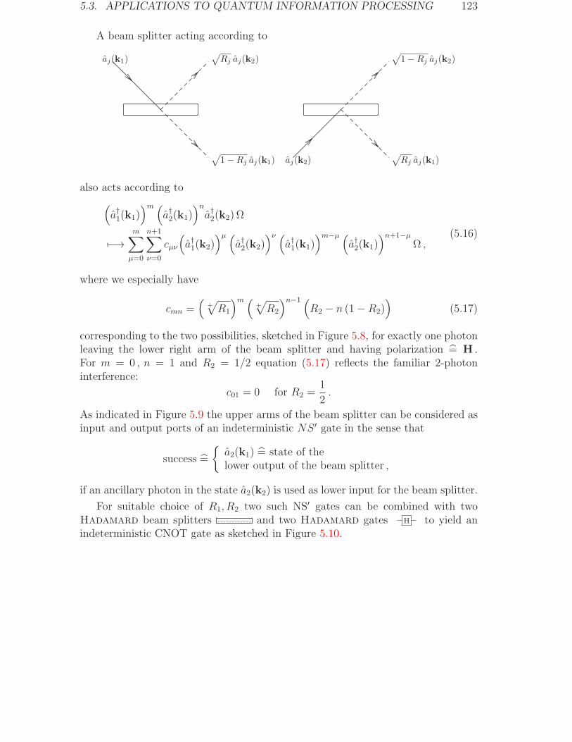
5.3. APPLICATIONS TO QUANTUM INFORMATION PROCESSING 123
A beam splitter acting according to
........
................................................
........................................
....................................
............
........
........................................
........
........................................ ........
........................................
√Rj aj(k2)aj(k1)
√1−Rj aj(k1) aj(k2)
√1−Rj aj(k2)
√Rj aj(k1)
..........................................................................................................................................................................................................
....................
....................
....................
....................
.
.....................................................................................................
....................
....................
....................
....................
....................
.
.....................................................................................................
......................................................................................................................................................................................
also acts according to
(a†1(k1)
)m (a†2(k1)
)na†2(k2) Ω
7−→m∑
µ=0
n+1∑
ν=0
cµν
(a†1(k2)
)µ (a†2(k2)
)ν (a†1(k1)
)m−µ (a†2(k1)
)n+1−µΩ ,
(5.16)
where we especially have
cmn =(
+√R1
)m (+√R2
)n−1 (R2 − n (1−R2)
)(5.17)
corresponding to the two possibilities, sketched in Figure 5.8, for exactly one photonleaving the lower right arm of the beam splitter and having polarization = H .For m = 0 , n = 1 and R2 = 1/2 equation (5.17) reflects the familiar 2-photoninterference:
c01 = 0 for R2 =1
2.
As indicated in Figure 5.9 the upper arms of the beam splitter can be considered asinput and output ports of an indeterministic NS ′ gate in the sense that
success =
a2(k1) = state of thelower output of the beam splitter ,
if an ancillary photon in the state a2(k2) is used as lower input for the beam splitter.
For suitable choice of R1, R2 two such NS′ gates can be combined with twoHadamard beam splitters ..................................... and two Hadamard gates H to yield anindeterministic CNOT gate as sketched in Figure 5.10.
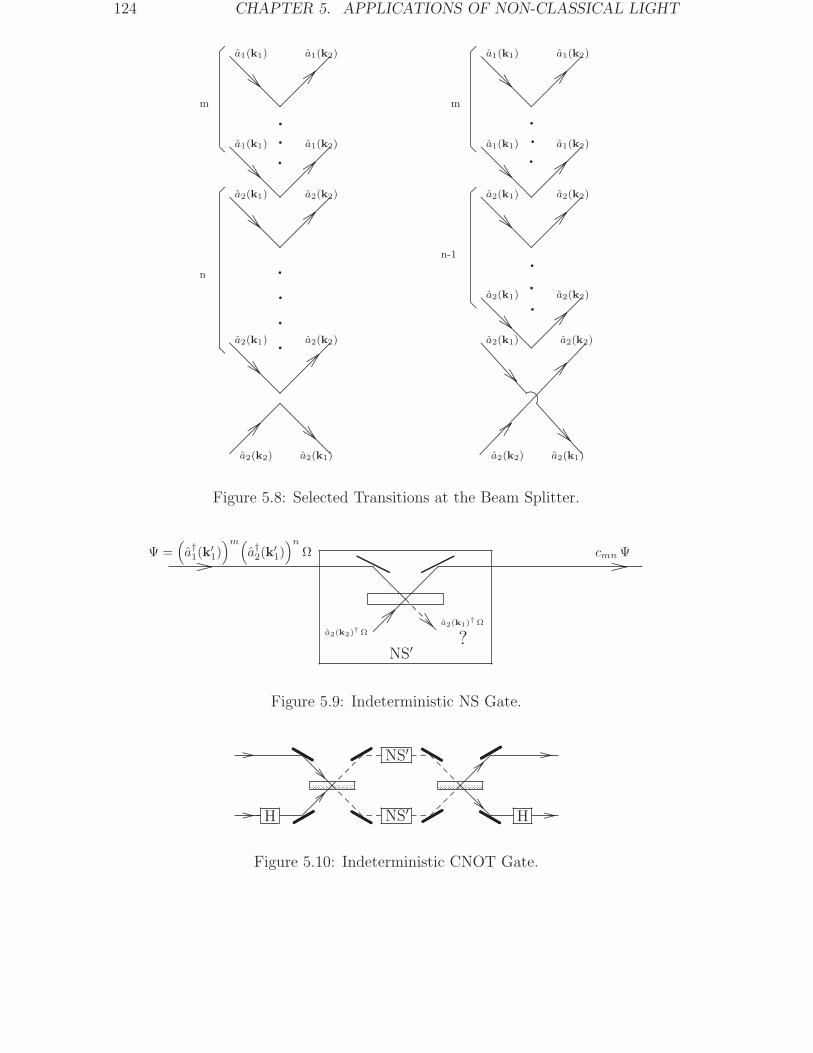
124 CHAPTER 5. APPLICATIONS OF NON-CLASSICAL LIGHT
.......................................
q
q
q
q
q
q
q
q
q
q
q
q
q
..............................................................................................................................................................................................................................................................................
.............................................
...................
..............................................................................................................................................................................................................................................................................
..............................................................................................................................................................................................................................................................................
..........
......................................................
.............................................
...................
..............................................................................................................................................................................................................................................................................
.............................................
...................
..........
......................................................
................................................................................................................................
................................................................................................................................
..........
......................................................
.............................................
...................
.............................................
...................
.................................................................................................................................................................................................................................................................................................
.............................................
...................
..............
..............
..............
..............
..............
..............
..............
..............
..........
......................................................
..........
......................................................
..........
......................................................
..........
......................................................
..........
....................................................
..........
......................................................
..........
......................................................
..........
....................................................
a1(k2)
a1(k1) a1(k2)
a1(k1)
a2(k1) a2(k2)
a1(k2)
a1(k1) a1(k2)
a1(k1)
a2(k1) a2(k2)
a2(k1) a2(k2)
a2(k2) a2(k1)
a2(k1)
a2(k2) a2(k1)
a2(k2)
a2(k1) a2(k2)
m
n-1
m
n
Figure 5.8: Selected Transitions at the Beam Splitter.
.......................................................................................
.............................................................................................................................................................................
....................
....................
.....................
.................................................................
..
........................................................
ppppppppppppppppppppppppppppppppppppppppppppppppppppppppppppppppppppp
ppppppppppppppppppppppppppppppppppppppppppppppppppppppppppppppppppppp....................................................
.............................
...............................
a2(k2)† Ω
a2(k1)† Ω
?NS′
Ψ =(a†1(k
′1))m(
a†2(k′1))n
Ω cmnΨ
Figure 5.9: Indeterministic NS Gate.
................................................ .................................................
qqqqqqqqqqqqqqqqqqqqqqqqqqqqqqqqqqqqqqqqqqqqqqqqqqqqqqqqqqqqqqqqqqqqqqqqqqqqqqqqqqqqqq
qqqqqqqqqqqqqqqqqqqqqqqqqqqqqqqqqqqqqqqqqqqqqqqqqqqqqqqqqqqqqqqqqqqqqqqqqqqqqqqqqqqqqq
qqqqqqqqqqqqqqqqqqqqqqqqqqqqqqqqqqqqqqqqqqq
qqqqqqqqqqqqqqqqqqqqqqqqqqqqqqqqqqqqqqqqqqqqqqqqqqqqqqqqqqqqqqqqqqqqqqqqqqqqqqqqqqqqqq
qqqqqqqqqqqqqqqqqqqqqqqqqqqqqqqqqqqqqqqqqqq
.................................................................................
.......... .......... ....................
....................
..........................................................................................
..................
..................
..................
..................
.........
................................................................................. .......... .......... .................................................
........................................
....................
.........
..............................
..........
..........
..........
.........
........
........................................
....................................
............
........
........................................
....................................
............
........................................
........................................
........................................
........................................
NS′
NS′
HH
Figure 5.10: Indeterministic CNOT Gate.
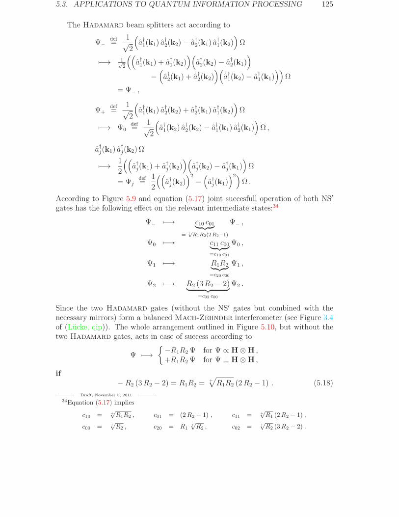
5.3. APPLICATIONS TO QUANTUM INFORMATION PROCESSING 125
The Hadamard beam splitters act according to
Ψ−def=
1√2
(a†1(k1) a
†2(k2)− a†2(k1) a
†1(k2)
)Ω
7−→ 1√2
((a†1(k1) + a†1(k2)
)(a†2(k2)− a†2(k1)
)
−(a†2(k1) + a†2(k2)
)(a†1(k2)− a†1(k1)
))Ω
= Ψ− ,
Ψ+def=
1√2
(a†1(k1) a
†2(k2) + a†2(k1) a
†1(k2)
)Ω
7−→ Ψ0def=
1√2
(a†1(k2) a
†2(k2)− a†1(k1) a
†2(k1)
)Ω ,
a†j(k1) a†j(k2) Ω
7−→ 1
2
((a†j(k1) + a†j(k2)
)(a†j(k2)− a†j(k1)
)Ω
= Ψjdef=
1
2
((a†j(k2)
)2−(a†j(k1)
)2)Ω .
According to Figure 5.9 and equation (5.17) joint succesfull operation of both NS′
gates has the following effect on the relevant intermediate states:34
Ψ− 7−→ c10 c01︸ ︷︷ ︸= +√R1R2(2R2−1)
Ψ− ,
Ψ0 7−→ c11 c00︸ ︷︷ ︸=c10 c01
Ψ0 ,
Ψ1 7−→ R1R2︸ ︷︷ ︸=c20 c00
Ψ1 ,
Ψ2 7−→ R2 (3R2 − 2)︸ ︷︷ ︸=c02 c00
Ψ2 .
Since the two Hadamard gates (without the NS′ gates but combined with thenecessary mirrors) form a balanced Mach-Zehnder interferometer (see Figure 3.4of (Lucke, qip)). The whole arrangement outlined in Figure 5.10, but without thetwo Hadamard gates, acts in case of success according to
Ψ 7−→−R1R2 Ψ for Ψ ∝ H⊗H ,+R1R2 Ψ for Ψ ⊥ H⊗H ,
if−R2 (3R2 − 2) = R1R2 =
+√R1R2 (2R2 − 1) . (5.18)
Draft, November 5, 2011
34Equation (5.17) implies
c10 = +√R1R2 , c01 = (2R2 − 1) , c11 = +
√R1 (2R2 − 1) ,
c00 = +√R2 , c20 = R1
+√R2 , c02 = +
√R2 (3R2 − 2) .
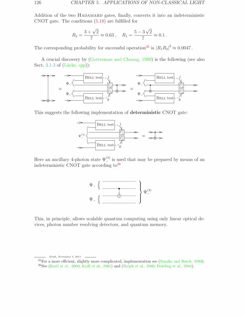
126 CHAPTER 5. APPLICATIONS OF NON-CLASSICAL LIGHT
Addition of the two Hadamard gates, finally, converts it into an indeterministicCNOT gate. The conditions (5.18) are fulfilled for
R2 =3 +
√2
7≈ 0.63 , R1 =
5− 3√2
7≈ 0.1 .
The corresponding probability for successful operation35 is |R1R2|2 ≈ 0.0047 .
A crucial discovery by (Gottesman and Chuang, 1999) is the following (see alsoSect. 3.1.3 of (Lucke, qip)):
Bell testBell test
.......
.......
...................................... ..........
...............
..........................................
....................
...............
.......
.......
...................................... ..........
...............
..........................................
....................
...............
r
...............................................
r
...............................................
r
................................................
....................
........................
..........................................
............................................
..........................................
..........................................
..........................................
....................
........................
..........................................
............................................
..........................................
..........................................
..........................................
..........................................
..........................................
..........................................
..........................................
≡
j
Ψ−
kBell testΨ−
j
Ψ−
kBell testΨ−
Uj
Uk
≡U ′j
U ′k
This suggests the following implementation of deterministic CNOT gate:
Bell test
.......
.......
...................................... ..........
...............
..........................................
....................
...............
...............................................
r
..........................................
..........................................
..........................................
..........................................
..........................................
..........................................
..........................................
..........................................
...........
......................
...........
j
kBell test
U ′j
U ′k
≡Ψ(4)−
Here an ancillary 4-photon state Ψ(4)− is used that may be prepared by means of an
indeterministic CNOT gate according to36
Ψ−
Ψ−
s
h
Ψ(4)−
This, in principle, allows scalable quantum computing using only linear optical de-vices, photon number resolving detectors, and quantum memory.
Draft, November 5, 2011
35For a more efficient, slightly more complicated, implementation see (Sanaka and Resch, 2003).36See (Knill et al., 2000; Knill et al., 2001) and (Ralph et al., 2002; Dowling et al., 2004).
Chapter 6
Coupling of Quantum Systems
Now it is customary to define the method of measuring physical quantities withoutdefining these quantities themselves. In fact we have no satisfactory reason for as-cribing objective existence to physical quantities as distinguished from the numbersobtained when we make the measurements which we correlate with them . . . It wouldevidently be philosophically more exact if we spoke of “making measurements” ofthis, that, or the other type instead of saying that we measure this, that, or the other“physical quantity” . . . however, we can continue to use the old language, reinter-preting the terms “physical quantity” and “dynamical variable,” and allowing themto stand for the corresponding operator which fixes the nature of the measurementunder consideration.
(Kemble, 1937, Section 36b)
6.1 Closed Systems
6.1.1 States and Observables in the Heisenberg Picture
In the Heisenberg picture the physical state of a closed1 quantum system ischaracterized by a density operator ρH on its state space H — being a Hilbert
space — and a time-dependent injection
Q 7−→ PHQ (t)
of the (naively assumed) testable ‘properties’ Q into the (orthogonal) projectorsPHQ (t) on H such that:2
pQ,t(ρH) def= Tr
(ρH PH
Q (t))=
probability for: “Q at time t” to beconfirmed by optimal tests .
(6.1)
Draft, November 5, 2011
1For a discussion of the applicability of the concept of a “closed system” (isolated system) see(Leggett, 2001, Lecture 3).
2If every step of a test for ‘Q at time t’ is delayed by ∆t then this amount to a test for ‘Q attime t+∆t’. We do not yet require that Q refers to an instant of time.
127
128 CHAPTER 6. COUPLING OF QUANTUM SYSTEMS
Remarks:
1. A density operator (statistical operator) is a positive traceclass operator ρ with
Tr(ρ) = 1
(see, e.g., Definition 8.3.19 of (Lucke, eine)).
2. The simplest density operators are those of the form
ρ = |Ψ〉〈Ψ| ,Ψ ∈ H ,
Those states are called vector states and fulfill 3
Tr(ρ P)=⟨Ψ | P Ψ
⟩=∥∥∥P Ψ
∥∥∥2
(6.2)
for all projectors P on Hfield .
3. Every density operator ρ on Hfield may be written in the form
ρ =∞∑
ν=1
λν︸︷︷︸≥0
|φν〉〈φν | ,∞∑
ν=1
λν = 1 = ‖Φµ‖ ∀µ ∈ N ,
suggesting the following naive interpretation:4
The actual state is one of the vector states φ1, φ2, . . . andλν is the probability for this being φν .
4. Note that (6.1) is assumed only over a time interval during whichthe system can be considered as closed. Thus, especially, the prepa-ration of the state has to be done before this time interval; andnontrivial tests (‘measurements’) — since inevitably changing thestate — are allowed only after this time interval.
5. More generally effects , i.e. bounded Operators A on H with 0 ≤A ≤ 1 , could be used5 instead of the projectors PH
Q (t) .
The (naive) idea behind (6.1) is the following:
• PHQ (t) projectsH onto the closed subspace corresponding to those vector states
for which “Q at time t” will be confirmed by every optimal test.
Draft, November 5, 2011
3Of course, Tr(ρ) = 1 implies ‖Ψ‖ = 1 .4In general, however, there is no unique choice for the states φν . See
(Timpson and Brown, 2005) in this connection.5See (Davies, 1976, Section 2.2), (Kraus, 1983, § 1), or (Busch et al., 1995) for the corresponding
physical interpretation.
6.1. CLOSED SYSTEMS 129
• ¬PHQ (t)
def= 1 − PH
Q (t) projects H onto the closed subspace corresponding tothose vector states for which “Q at time t” will never be confirmed by anyoptimal test.
• Since∥∥∥PH
Q (t)Ψ∥∥∥2
+∥∥∥¬PH
Q (t)Ψ∥∥∥2
= 1 it seems natural to interpret
∥∥∥PHQ (t)Ψ
∥∥∥2
= Tr(|Ψ〉〈Ψ| PH
Q (t))
as the probability for “Q at time t” in a state described by ρH = |Ψ〉〈Ψ| .
• This motivates (6.1) for vector states.
• Due to linearity of the trace this implies (6.1) for states represented by densityoperators of the form
ρH =∞∑
ν=0
pν︸︷︷︸≥0
|Ψ〉ν〈Ψ|ν ,∞∑
ν=0
pν = 1 , (6.3)
if,6 for every ν , pν is (naively) identified with the probability for the systemto be in the vector state corresponding to Ψν .
• Since every density operator can be written in the form (6.3), thanks to theHilbert-Schmidt theorem (see, e.g., Corollary 8.3.18 of (Lucke, eine)), thisimplies (6.1) for all states.
There is a one-one correspondence between self-adjoint operators A (see, e.g., Defi-
nition 8.3.7 (Lucke, eine)) and familiesEAλ
λ∈R
of projectors fulfilling the following
requirements (see Theorem 8.3.24 of (Lucke, eine)):
1. (λ1 ≤ λ2 =⇒
⟨Ψ | EA
λ1Ψ⟩≤⟨Ψ | Eλ2Ψ
⟩)∀Ψ ∈ H , λ1, λ2 ∈ R .
2.limǫ→−∞
⟨Ψ | EA
λΨ⟩= 0 ∀Ψ ∈ H , λ ∈ R .
3.limǫ→+∞
⟨Ψ | EA
λΨ⟩= 〈Ψ | Ψ〉 ∀Ψ ∈ H , λ ∈ R .
4.limǫ→+0
⟨Ψ | EA
λ+ǫΨ⟩=⟨Ψ | EA
λΨ⟩
∀Ψ ∈ H , λ ∈ R .
Draft, November 5, 2011
6See also Section 6.2.2 and (Zeh, 2000) for mixed states arising for subsystems from vectorstates of a composed system.
130 CHAPTER 6. COUPLING OF QUANTUM SYSTEMS
5.
DA =
Ψ ∈ H :
∫|λ|2 d
⟨Ψ | EA
λ Ψ⟩<∞
.
6. ⟨Ψ | AΨ
⟩=
∫λ d⟨Ψ | EA
λ Ψ⟩
∀Ψ ∈ DA .
Therefore self-adjoint operators are interpreted as observables of physical quanti-ties — like ‘energy at time t’ — in the following sense:
Tr(ρH EA
λ
)=
probability for: “A ∈ (−∞, λ]” to beconfirmed by optimal tests .
Consequently:
Tr(ρH A
)= expectation value of A in the state = ρH . (6.4)
Projectors are just observables of physical quantities for which only 0 and 1 are‘possible values’.
6.1.2 Time Evolution and Projective Measurements
For a closed quantum system the time evolution is assumed to be given by a self-adjoint operator H called the Hamiltonian of the system, in the sense that
PHQ (t) = e+
i~H t PH
Q (0) e− i
~H t ∀ t ∈ R (6.5)
holds for all ‘testable properties’ Q .
Remark: See, e.g., (Lucke, 1996, Section2.5) for a justification of this assumptionand Definition 8.3.30 of (Lucke, eine) for the definition of functions of self-adjointoperators.
This allows switching to the Schrodinger picture
Tr(ρSt P
SQ
)=
probability for “Q at time t” to beconfirmed by optimal tests ,
(6.6)
where
ρStdef= e−
i~H t ρH e+
i~H t , (6.7)
P SQ
def= PH(0)
= e−i~H t PH
Q (t) e+ i
~H t . (6.8)
6.1. CLOSED SYSTEMS 131
Note that, formally, (6.7) is equivalent to the Liouville equation
i~∂
∂tρSt =
[H , ρSt
]−
(6.9)
— to be suitably interpreted.
If the Hamiltonian is of the form
H = H0 + V (6.10)
with e−i~H0 t known and V ‘small’ in some sense then it may be convenient to switch
to the interaction picture
Tr(ρIt P
IQ(t)
)=
probability for “Q at time t” to beconfirmed by optimal tests ,
(6.11)
where
ρItdef= e+
i~H0 t e−
i~H t ρH e+
i~H t e−
i~H0 t , (6.12)
P IQ(t) = e+
i~H0 t PH
Q (0) e− i
~H0 t . (6.13)
The reason will become evident in Section 6.1.3.
For simplicity we require that for every ‘testable property’ Q there is a projec-tive measurement , i.e. a test changing the Heisenberg state according to7
ρH 7−→ pQ,t(ρH)ρHQ,t +
(1− pQ,t
(ρH))ρH¬Q,t (6.14)
with
ρHQ,tdef=
PHQ (t)ρ
HPHQ (t)
Tr(PHQ (t)ρ
HPHQ (t)
)
describing the subensemble of all those individual systems for which ‘Q at time t’has been confirmed and
ρH¬Q,tdef=
PH¬Q(t)ρ
HPH¬Q(t)
Tr(PH¬Q(t)ρ
HPH¬Q(t)
) , PH¬Q(t) = 1− PH
Q (t) ,
describing the subensemble of all those individual systems for which ‘Q at time t’ isdenied by the test. This assumption is consistent in the sense that
Tr(ρH)= Tr
(pQ,t(ρH)ρHQ,t +
(1− pQ,t
(ρH))ρH¬Q,t
).
Draft, November 5, 2011
7Recall (6.1).
132 CHAPTER 6. COUPLING OF QUANTUM SYSTEMS
Note that
pQ′,t
(ρH)= pQ′,t
(pQ,t(ρH)ρHQ,t +
(1− pQ,t
(ρH))ρH¬Q,t
)∀ ρH
⇐⇒[PHQ (t) , P
HQ′(t)
]−= 0 ,
sinceTr(ρ A)= Tr
(A ρ)
(6.15)
holds for all trace class operators ρ and all bounded operators A . Therefore ‘testableproperties’ Q , Q′ with commuting PH
Q (t) , PHQ′(t) are called compatible .8
6.1.3 Time Dependent Perturbation Theory9
In the interaction picture the time-dependent density operator (6.12) fulfills thedifferential equation10
i~d
dtρIt =
[V I(t), ρIt
]−, (6.16)
whereV I(t)
def= e+
i~H0 t V e−
i~H0 t . (6.17)
(6.16) is (formally) equivalent to the integral equation
ρIt = ρI0 −i
~
∫ t
0
[V I(t′), ρIt′
]−dt′
which may be solved for given ρI0 by iteration
ρ(0)t
def= ρI0 ,
ρ(ν)t
def= ρI0 −
i
~
∫ t
0
[V I(t′), ρ(ν−1)
t′
]−dt′ for ν = 1, 2, . . .
(6.18)
and taking the limit11
ρIt = limν→∞
ρ(ν)t
Draft, November 5, 2011
8Note that
[PHQ (0) , PH
Q′(0)]−= 0 ⇐⇒
(6.5)
([PHQ (t) , PH
Q′(t)]−= 0 ∀ t ∈ R
).
9In this subsection we do not care about mathematical details since even for a divergent per-turbative expansion the lowest order may provide useful results.
10Compare Equation (6.9).11For simplicity, we do not specify the type of convergence.
6.2. BIPARTITE SYSTEMS 133
if V I(t) is ‘sufficiently small’. For typical applications the approximation
ρIt ≈ ρ(2)t = ρI0 −
i
~
∫ t
0
[V I(t′), ρI0
]−dt′
−~−2
∫ t
0
(∫ t′
0
[V I(t′),
[V I(t′′), ρI0
]−
]
−dt′′)dt′
is good enough. Note that, thanks to (6.15),
P ρI0 = ρI0 P = 0
=⇒ Tr(ρ(2)t P
)= ~
−2
∫
[0,t]×[0,t]
Tr(V I(t′) ρI0 V
I(t′′) P)dt′′ dt′ .
(6.19)
This is in agreement with Dyson’s perturbation theory for state vectors.12
6.2 Bipartite Systems
6.2.1 Composition of Distinguishable Systems
Let S1 and S2 be distinguishable quantum systems not interacting with eachother. In order to describe S1 and S2 together as a single quantum system S in theHeisenberg picture one takes the state space H = H1 ⊗H2 , where H1 resp. H2 isthe state space of S1 resp. S2 .
Remark: See, e.g., Section 8.4.2 of (Lucke, eine) for the definition of the tensorproducts ⊗ .
The Hamiltonian of S isH = H1 ⊗ 1 + 1⊗ H2 , (6.20)
where H1 resp. H2 is the Hamiltonian of S1 resp. S2 , and therefore
e+i~H t(PHQ1(0)⊗ PH
Q2(0))e−
i~H t = PH
Q1(t)⊗ PH
Q2(t) ∀ t ∈ R (6.21)
holds for all ‘testable properties’ Q1 and Q2 of S1 resp. S2 .
If the Heisenberg state of S is given by
ρH = ρH1 ⊗ ρH2 (6.22)
thenTr(ρH(PHQ1(t)⊗ PH
Q2(t)))
= Tr(ρH1 P
HQ1(t))Tr(ρH2 P
HQ2(t)).
This suggests the interpretation
Tr(ρH(PHQ1(t)⊗ PH
Q2(t)))
=
probability for: “Q1 and Q2 at time t”to be confirmed by optimal tests .
(6.23)
Draft, November 5, 2011
12See Appendix A.4.
134 CHAPTER 6. COUPLING OF QUANTUM SYSTEMS
As long as (6.20) holds (6.23) is equivalent to
Tr(ρSt
(P SQ1
⊗ P SQ2
))=
probability for: “Q1 and Q2 at time t”to be confirmed by optimal tests ,
(6.24)
thanks to (6.21). However, if an interaction between S1 and S2 is introduced, cor-responding to the addition of a perturbation
V 6= V1 ⊗ 1 + 1⊗ V2 ∀ V1 , V2 (6.25)
on the r.h.s. of (6.20), then (6.21) is no longer consistent for all Q1, Q2 . Then wetry to keep (6.24) for as many Q1, Q2 as possible.13
Even for the restricted class of Q1, Q2 do correlations arise, i.e.
Tr(ρSt
(P SQ1
⊗ P SQ2
)) i.g.
6= Tr(ρSt
(P SQ1
⊗ 1))
Tr(ρSt
(1⊗ P S
Q2
)),
since:
Even if the Schrodinger state at time 0 is factorized , i.e. if
ρS0 = ρ1 ⊗ ρ2 ,
ρSt is typically not even separable14 for t > 0 .
Correlations of subsystems also arise for classical systems. But:
The subsystems S1 , S2 of S should be considered as classically cor-related at time t only if ρSt is separable (Werner, 1989).
6.2.2 Partial States
Now let us consider a bipartite system S as described in 6.2.1 and ask only forproperties Q1 of the subsystem S , i.e. for the partial state of S1 given by themapping
(Q1, t) 7−→ Tr(ρSt
(P SQ1
⊗ 1))
=
probability for: “Q1 at time t”to be confirmed by optimal tests .
.
Draft, November 5, 2011
13Problems arise whenever the relation between two observables depends on the dynamics; atypical example being the observables of position and velocity.
14A (momentary Schrodinger) state with density operator ρ is called separable if for everyǫ > 0 there exist N ∈ N , p1, . . . , pN ≥ 0 , and density operators ρ1,ν , . . . , ρ2,N with
Tr
∣∣∣∣∣ρ−N∑
ν=1
pν ρ1,ν ⊗ ρ2,ν
∣∣∣∣∣ < ǫ .
Otherwise the state is called entangled.
6.2. BIPARTITE SYSTEMS 135
One may show that (for every t) there is a density operator Tr2(ρSt)on H1 , called
the partial trace of ρSt w.r.t. H2 , for which
Tr(ρSt
(P SQ1
⊗ 1))
= Tr(Tr2(ρSt)P SQ1
)∀Q1 . (6.26)
Obviously, Tr2(ρSt)represents the partial Schrodinger state of S1 at time t . But:
Even if ρSt represents a vector state of S its partial trace w.r.t. H2 usuallydoes not represent a vector state15 of S1 .
Moreover, the interaction between S1 and S2 has to be very special16 for all theTr2(ρSt)with t > 0 to be determined by Tr2
(ρS0), at all. Usually, therefore, the
Heisenberg picture does not work for subsystems.
6.2.3 Composition of Indistinguishable Systems
Two quantum systems S1 , S2 are called indistinguishable if they may be de-scribed in the same way, especially with
H1 = H2 , H1 = H2 , Q1 = Q2 .Then there is a natural decomposition
H1 ⊗H2 = H+ ⊕H− ,
where Hσ denotes the Hilbert subspace of H1 ⊗H2 generated by all vectors Ψ ofthe form
Ψ = ψ1 ⊗ ψ2 + σψ2 ⊗ ψ1 , ψ1, ψ2 ∈ H1 ,
and the composition described in 6.2.1 has to be modified in the following way:17
1. The state space of the composed system is Hσ with σ = +resp. σ = − if S1 isa Boson resp. a Fermion .
2. Only those properties of the composed system can be considered as ‘testableproperties’ which do not depend on the enumeration of the subsystems. Thus,for instance, if Q1 6= Q2 are compatible properties of S1 then
(‘Q1 for S1’ ∧ ‘Q2 for S2’) ∨ (‘Q2 for S1’ ∧ ‘Q1 for S2’)
is a ‘testable property’ of the composed system represented by the projector(P SQ1
⊗ P SQ2
+ P SQ2
⊗ P SQ1
−(P SQ1P SQ2
)⊗(P SQ1P SQ2
))/\Hσ
in the Schrodinger picture. But
‘Q1 for S1’ ∧ ‘Q2 for S2’
cannot be considered as a testable.
Draft, November 5, 2011
15The evolution of an initial partial vector state into a mixed state is called decoherence.16See Section 6.317Here we assume V = 0 , for simplicity.
136 CHAPTER 6. COUPLING OF QUANTUM SYSTEMS
3. The Hamiltonian has to be replaced by
(H1 ⊗ 1 + 1⊗ H2 + V
)/\Hσ
with V leaving Hσ invariant.
Recall that particles with integer spin like photons are Bosons while particles withhalf-integer spin like electrons are Fermions.
For multipartite systems and the possibility of parastatistics we refer to (Ohnuki and Kamefuchi, 1982

6.3. OPEN SYSTEMS 137
6.3 Open Systems
See (Davies, 1976; Kraus, 1983; Carmichael, 1993; Alicki, 2003).

138 CHAPTER 6. COUPLING OF QUANTUM SYSTEMS
Chapter 7
Perturbation Theory of RadiativeTransitions
Being able to predict things or describe them, however accurately, is not at all thesame thing as understanding them.
(Deutsch, 1997, p. 2)
7.1 Single Atoms in General
7.1.1 Naive Interaction Picture
Let S1 be a single 1-electron atom with approximate Hamiltonian1
Hatomdef=
p 2can
2m+ qcA0(x)
acting on Hatom = L2(R3) and let S2 be the electromagnetic radiation system withstate space Hfield and Hamiltonian
Hfield =1
2
∫ (ǫ0 : E⊥(x, 0) · E⊥(x, 0) : +
1
µ0
: B(x, 0) · B(x, 0) :
)dVx ,
where E⊥(x, 0) resp. B(x, 0) denotes the observable of the electric2 resp. magneticfield at time t = 0 .
Draft, November 5, 2011
1We assume that the atom’s center of mass fixed at x = 0 and neglect spin-orbit interactionand the like. q < 0 is the electron’s charge, m > 0 its (reduced) mass , c ≈ 3 · 10−10cm the velocityof light in vacuum, and cA0(x) the electric (binding) potential of the nucleus. pcan denotes theelectron’s canonical momentum operator and x its position operator:
(pjcan ψ
)(x) =
~
i
∂
∂xjψ(x) ,
(xj ψ
)(x) = xj ψ(x) .
2Note that only in the absence of charges the total electric field E(x, 0) coincides with its
transversal part E⊥(x, 0) (recall Footnote 33 of Chapter 1).
139
140 CHAPTER 7. RADIATIVE TRANSITIONS
Agreement: From now on we identify operators B on Hatom with thecorresponding operators B⊗ 1field on Hatom⊗Hfield . Similarly we identifyoperators C on Hfield with the corresponding operators 1atom ⊗ C onHatom ⊗Hfield .
Since the interaction between S1 and S2 cannot be switched off let us considerthese systems as components of a closed bipartite system, as described in 6.2.1, withminimal coupling3
V = − q
2m
(pcan · A (x, 0) + A (x, 0) · pcan
)
+q2
2m:A 2(x, 0) : ,
(7.1)
where we assume that the naive interaction picture works, i.e. that the state spaceand the time zero fields E⊥(x, 0) , B(x, 0) , A(x, 0) can be chosen identical withthose of the free theory described in 1.2.2.
Warning: Actually, as stressed in (Hoffmann, 1994, Sect. 3.5), V is notwell-defined. This is a simple consequence of the equations
Aj10 (x1, t1) Aj20 (x2, t2) = : Aj10 (x1, t1) A
j20 (x2, t2) :
+⟨Ω | Aj10 (x1, t1) A
j20 (x2, t2) Ω
⟩ (7.2)
and⟨Ω | Aj10 (x1, t1) A
j20 (x2, t2) Ω
⟩
=
⟨Ω |[(Aj10 )
(+)(x1, t1) ,((Aj20 )
(+)(x2, t2))†]
−Ω
⟩
=(1.45)
(2π)−3 µ0 ~ c
∫ (δj1j2 −
kj1kj2
|k|2)eik(x1−x2) e−i c|k|(t1−t2)
dVk2 |k|
(7.3)for the free field operators A0(x, t) . Therefore we should replace A(x, 0)
by
∫A0(x−y, 0)ϕ(y) dy with ϕ ∈ S(R3) (introduce a ultraviolet cutoff
this way) and determine the limit dynamics for ϕ→ δ . However, we arenot going to elaborate on such mathematical details.4
Draft, November 5, 2011
3Our notation should be understood in the sense that, e.g.,
⟨ψ′ ⊗ χ′ | A (x, 0) (ψ ⊗ χ)
⟩def=
∫ (ψ′(x)
)∗ψ(x)
⟨χ′ | A (x, 0) χ
⟩field
dVx
holds for sufficiently well-behaved ψ ⊗ χ, ψ′ ⊗ χ′ ∈ H . See (Simon, 1971) in this context.4See (Frohlich et al., 2003) for such techniques.
7.1. SINGLE ATOMS IN GENERAL 141
Remark: (7.2) is a special case ofWick’s theorem; see, e.g., Sect. 3.2.1 of (Lucke, qft).
Now the time evolution of the composed system is generated by the total Hamilto-nian
H = Hatom + Hfield + V (7.4)
=1
2m:(pcan − q A(x, 0)︸ ︷︷ ︸= pkin
def= m i
~[H,x]−
)2: + qcA0(x) + Hfield . (7.5)
For (sufficiently well-behaved) vector states the dynamical law (6.7) suggestsvalidity of the Schrodinger equation5
i~d
dtΨt = H Ψt ∀ t ∈ R , (7.6)
where ρSt = |Ψt〉〈Ψt| .Remark: See Section 9.1.1 of (Lucke, eine) for arbitrary vector states.
Assuming6
Ψt ≈ ψt ⊗ χt ,‖χt‖ = 1
∀ t ∈ R (7.7)
and taking the inner product of (7.6) with ψ′ ⊗ χt gives
∫ (ψ′(x)
)∗i~
∂
∂tψt(x) dVx
=⟨ψ′ ⊗ χt
∣∣∣ i~ d
dt(ψt ⊗ χt)
⟩− 〈ψ′ | ψt〉
⟨χt
∣∣∣i~ d
dtχt
⟩
≈(7.7),(7.6)
⟨ψ′ ⊗ χt | H (ψt ⊗ χt)
⟩− 〈ψ′ | ψt〉
⟨χt
∣∣∣i~ d
dtχt
⟩
=(7.4),(7.1)
⟨ψ′ | Hatom ψt
⟩+ 〈ψ′ | ψt〉
⟨χt
∣∣∣(Hfield − i~
d
dt
)χt
⟩
− q
2m
∫ (ψ′(x)
)∗(pcan ·Aext(x, t) +Aext(x, t) · pcan)ψt(x) dVx
+q2
2m
∫ (ψ′(x)
)∗ ⟨χt
∣∣∣ :A 2(x, 0) :χt
⟩ψt(x) dVx ,
whereAext(x, t)
def=⟨χt | A(x, 0)χt
⟩.
Draft, November 5, 2011
5Note, however, that the time evolution of ρSt — contrary to that of Ψt — is not changed byaddition of a constant to H .
6This possibility seems reasonable for coherent states χ0 ; see end of 7.2.1.
142 CHAPTER 7. RADIATIVE TRANSITIONS
Since ψ′ is arbitrary, this establishes the exterior field formalism
i~∂
∂tψt(x) ≈
(1
2m
(~
i∇− qAext(x, t)
)2
+ qcA0ext(x, t) + qcA0(x)
)ψt(x) , (7.8)
if (7.7) holds ,
with suitably defined A0ext(x, t) . We postpone the discussion under which conditions
(7.7) is reasonable.7
7.1.2 Electric Field Representation8
Let us choose some ϕ ∈ S (R3) with
ϕ(x) =(ϕ(x)
)∗≈ δ(x) (7.9)
and exploit the Wigner symmetry corresponding to the unitary operator
U = exp
(− i
~q x ·
∫A(y, 0)ϕ(y) dy
). (7.10)
Remark: See,e.g., Section 8.3.4 of (Lucke, eine) for the notion of Wigner symme-try.
This means that all operators B have to be replaced by
AdU Bdef= U B U−1 (7.11)
without changing the physical interpretation. The new observable for the transversalpart of the electric field, for example, in the Schrodinger picture is now
AdU E⊥(x, 0) = E⊥(x, 0)−1
ǫ 0P
(0)⊥ (x) , (7.12)
where
P(0)⊥ (x)
def= ǫ0
3∑
j=1
q xji
~
∫ [Aj(y, 0), E⊥(x, 0)
]−ϕ(y) dy . (7.13)
Proof of (7.12): As usual, we (formally) define
adA Bdef=[A, B
]−.
Draft, November 5, 2011
7See (Gemmer and Mahler, 2001) for the case of bipartite systems with finite dimensional statespaces.
8Here we follow (Cohen-Tannoudji et al., 1992, Appendix 5), to some extent, rather than(Mandel and Wolf, 1995, Section 14.1.3). See also (Scully and Zubairy, 1999, App. 5.A) for thecorresponding exterior field formalism.
7.1. SINGLE ATOMS IN GENERAL 143
Then (1.37) implies that adln(U)E⊥(x, 0) is a function of x and, conse-quently, (
adln(U)
)νE⊥(x, 0) = 0 ∀ ν > 1 .
Therefore (7.12) follows from the Campbell-Hausdorff formula9
Adexp(A) B = exp(adA) B (7.14)
and
adln(U)E⊥(x, 0) = − i
~q
3∑
j=1
xj∫ [
Aj(y, 0), E⊥(x, 0)]−ϕ(y) dy .
Similarly we get:
AdU x = x ,
AdU pkin = pkin + qi
~
3∑
j=1
[pcan, x
j]−
∫Aj(y, 0)ϕ(y) dy
= pcan − q A (x, 0) + q
∫A(y, 0)ϕ(y) dy (7.15)
AdUB(x, 0) =(1.48)
B(x, 0) ,
AdUH =1
2m: (AdU pkin)
2 : + qcA0(x) + Hfield
−∫
P(0)⊥ (x) · E⊥(x, 0) dVx +
1
2ǫ0
∫ (P
(0)⊥ (x)
)2dVx .(7.16)
Proof of (7.16): According to (7.5) it is sufficient to show
AdU Hfield = Hfield −∫
P(0)⊥ (x) · E⊥(x, 0) dVx +
1
2ǫ0
∫ (P
(0)⊥ (x)
)2dVx .
This follows from
AdU Hfield =1
2
∫ (ǫ0 :
(AdU E⊥(x, 0)
)2: +
1
µ0: B2(x, 0) :
)dVx
and (7.12).
Draft, November 5, 2011
9Formally (7.14) is a consequence of the fact that Adexp(λA) B and exp(adλA
)B , considered as
operator-valued functions of λ , fulfill the same first order differential equation and the same initialcondition for λ = 0 .
144 CHAPTER 7. RADIATIVE TRANSITIONS
Note that (1.49) and (7.13) imply10
P(0)⊥ (x) = q
3∑
j,j′=1
xj ej′
∫δjj
′
⊥ (y − x)ϕ(y) dy . (7.17)
Since ∫δjj
′
⊥ (y − x) Ej′
⊥(x) dVx = Ej⊥(y) ,
(7.17) implies
∫P
(0)⊥ (x) · E⊥(x, 0) dVx = q x ·
∫E⊥(y, 0)ϕ(y) dy .
Substituting the latter into (7.16) we get
AdUH =
(1
2m: (AdU pkin)
2 : + qcA0(x) +1
2ǫ0
∫ (P
(0)⊥ (x)
)2dVx
)+ Hfield
−q x ·∫
E⊥(y, 0)ϕ(y) dy .
(7.18)Therefore we call the new representation, resulting from the Wigner symmetrytransformation AdU , the electric field representation .
Warning: The new observable of the (transversal part of the) electricfield is AdU E⊥(x, 0) rather than E⊥(x, 0) . According to (7.12)/(7.13),both coincide only ‘outside’ the atom.
7.1.3 First Order Perturbation Theory
Let us go back to the representation described in 7.1.1 which we shall call theCoulomb representation . Then we have
H0def= Hatom + Hfield
Draft, November 5, 2011
10The observable of the transversal polarization density is the operator-valued distribution
P⊥(x)def= q
3∑
j,j′=1
xj ej′δjj′
⊥ (x− x)
= ǫ0
3∑
j=1
q xji
~
[Aj(x, 0), E⊥(x, 0)
]−.
7.1. SINGLE ATOMS IN GENERAL 145
as unperturbed Hamiltonian and
V I(t) =(6.17)
e+i~H0 t V e−
i~H0 t
with V given by (7.1).
Let us consider the special case
ρI0 = |ψ ⊗ χ〉〈ψ ⊗ χ| ,P =
∣∣ψ ⊗ χ⟩⟨ψ ⊗ χ
∣∣ ,P ρI0 = ρI0 P = 0 .
(7.19)
Then11
pt(ψ ⊗ χ→ ψ ⊗ χ
)
def= Tr
(ρIt P
)
≈(6.19)
~−2
∣∣∣∣∫ t
0
⟨ψ ⊗ χ | V I(t′) (ψ ⊗ χ)
⟩dt′∣∣∣∣2
=(6.17)
~−2
∣∣∣∣∫ t
0
⟨ψ
(0)t′ ⊗ χ
(0)t′ | V
(ψ
(0)t′ ⊗ χ
(0)t′
)⟩dt′∣∣∣∣2
=(7.1)
~−2
∣∣∣∣∫ t
0
(− q
m
∫ 3∑
j=1
⟨χ(0)t′ | Aj(x, 0)χ(0)
t′
⟩(ψ
(0)t′ (x)
)∗ ~i
∂
∂xjψ
(0)t′ (x) dVx
+q2
2m
∫ ⟨χ(0)t′ | :A2(x, 0) :χ
(0)t′
⟩(ψ
(0)t′ (x)
)∗ψ
(0)t′ (x) dVx
)dt′∣∣∣∣2
,
= ~−2
∣∣∣∣∫ t
0
(− q
m
∫ 3∑
j=1
⟨χ | Aj(x, t′)χ
⟩(ψ
(0)t′ (x)
)∗ ~i
∂
∂xjψ
(0)t′ (x) dVx
+q2
2m
∫ ⟨χ | :
(A)2(x, t′) :χ
⟩(ψ
(0)t′ (x)
)∗ψ
(0)t′ (x) dVx
)dt′∣∣∣∣2
,
where we usedA(x, t) = e+
i~Hfield t A(x, 0) e−
i~Hfield t (7.20)
andψ
(0)t
def= e−
i~Hatom t ψ , ψ
(0)t
def= e−
i~Hatom t ψ ,
χ(0)t
def= e−
i~Hfield t χ , χ
(0)t
def= e−
i~Hfield t χ .
Draft, November 5, 2011
11Note that ∇ · A(x, 0) = 0 .
146 CHAPTER 7. RADIATIVE TRANSITIONS
Usually
⟨χ | :
(A)2(x, t′) :χ
⟩will be neglected:12
pt(ψ ⊗ χ→ ψ ⊗ χ
)
≈ q2
m2~2
∣∣∣∣∣
∫ t
0
(∫ 3∑
j=1
⟨χ | Aj(x, t′)χ
⟩(ψ
(0)t′ (x)
)∗ ~i
∂
∂xjψ
(0)t′ (x) dVx
)dt′
∣∣∣∣∣
2
if (7.19) holds .
(7.21)
For obvious reasons13
pt(ψ ⊗ χ→ ψ ⊗ χ
)=
(6.7),(6.12)Tr(ρSt e
− i~H0 t P e+
i~H0 t)
is called the transition probability for the transition of the Schrodinger state= e−
i~H0 t (ψ ⊗ χ) into the Schrodinger state = e−
i~H0 t(ψ ⊗ χ
)at time t .
In typical quantum optical applications also the approximation∫ 3∑
j=1
⟨χ | Aj(x, t′)χ
⟩(ψ
(0)t′ (x)
)∗ ~i
∂
∂xjψ
(0)t′ (x) dVx
≈∫ 3∑
j=1
⟨χ | Aj(0, t′)χ
⟩(ψ
(0)t′ (x)
)∗ ~i
∂
∂xjψ
(0)t′ (x) dVx
=⟨χ | A(0, t′)χ
⟩·⟨ψ
(0)t′ | pcan ψ
(0)t′
⟩
=⟨χ | A(0, t′)χ
⟩·⟨ψ
(0)t′ | m i
~
[Hatom, x
]−ψ
(0)t′
⟩
=m
q
⟨χ | A(0, t′)χ
⟩· d
dt′
⟨ψ
(0)t′ | q xψ(0)
t′
⟩
is justified. Substituting this into (7.21) we get the so-called electric dipoleapproximation
pt(ψ ⊗ χ→ ψ ⊗ χ
)
≈∫
[0,t]2
3∑
j1,j2=1
⟨χ | Aj1(0, t1) χ
⟩⟨χ | Aj2(0, t2)χ
⟩f j1j2ψ,ψ
(t1, t2) dt1 dt2 ,
in the Coulomb representation, where
f j1j2ψ,ψ
(t1, t2)def= ~
−2
(d
dt1
⟨ψ
(0)t1 | q xj1 ψ(0)
t1
⟩)( d
dt2
⟨ψ
(0)t2 | q xj2 ψ(0)
t2
⟩).
(7.22)
Obviously, the f -factor gives rise to selection rules :14⟨ψ
(0)t′ | q xψ(0)
t′
⟩= 0 ∀ t′ ∈ [0, t] =⇒ pt
(ψ ⊗ χ→ ψ ⊗ χ
)≈ 0 . (7.23)
Draft, November 5, 2011
12See (Mandel and Wolf, 1995, End of Section 14.1.2) for justification.13Recall (6.6).14The l.h.s. of (7.23) is often implied by symmetries.
7.2. PHOTOELECTRIC DETECTION OF LIGHT 147
Remark: Note that⟨χ | A(x, t) Ω
⟩ i.g.
6= 0(=⟨Ω | A(x, t) Ω
⟩).
Therefore (7.22) may be non-negligible even for χ = Ω . This explains,e.g., the occurrence of spontaneous decay15 of excited atomic states inthe vacuum.
7.2 Photoelectric Detection of Light
7.2.1 Ionisation of One-Electron Atoms
Let us assume that the projection Pion onto the subspace of Hatom corresponding toionisation is of the form
Pion =
∫
E≥0
σ(E, Ω)︸ ︷︷ ︸≥0
∣∣ψ(E, Ω)⟩⟨ψ(E, Ω)
∣∣ dE dΩ , (7.24)
where the ψ(E, Ω) are (improper) eigenstates of Hatom :
Hatom ψ(E, Ω) = E ψ(E, Ω) .
Moreover, let χνν∈N be a maximal orthonormal system (MONS) of Hfield . Then,if
Hatom ψ = E ψ , E < 0 ,
the probability piont (ψ, χ) for ionisation at time t is
piont (ψ, χ)
= Tr(ρIt
(Pion ⊗ 1
))
=∞∑
ν=1
∫
E≥0
σ(E, Ω) pt(ψ ⊗ χ→ ψ(E, Ω)⊗ χν
)dE dΩ
≈(7.22)
∫
[0,t]2
3∑
j1,j2=1
⟨χ | Aj1(0, t1) Aj2(0, t2)χ
⟩Ij1j2ψ (t1 − t2) dt1 dt2 ,
where
Ij1j2ψ (t1 − t2)
def=
∫
E≥0
σ(E, Ω)(E − E
)2 ⟨ψ | q xj1 ψ(E, Ω)
⟩⟨ψ(E, Ω) | q xj2 ψ
⟩·
· e+ i~(E−E)(t1−t2) dE dΩ
=
∫
E≥0
σ(E, Ω) f j1j2ψ,ψ(E,Ω)
(t1, t2) dE dΩ .
Draft, November 5, 2011
15See, e.g., (Baym, 1969, Chapter 13).
148 CHAPTER 7. RADIATIVE TRANSITIONS
This together with (7.2) gives
piont (ψ, χ)
≈∫
[0,t]2
3∑
j1,j2=1
⟨χ | : Aj1(0, t1) Aj2(0, t2) :χ
⟩Ij1j2ψ (t1 − t2) dt1 dt2 + Vt(ψ) , (7.25)
where
Vt(ψ) def=
∫
[0,t]2
3∑
j1,j2=1
⟨Ω | Aj1(0, t1) Aj2(0, t2) Ω
⟩Ij1j2ψ (t1 − t2) dt1 dt2
=(7.3)
(2π)−3 µ0 ~ c3∑
j1,j2=1
∫ (δj1j2 −
kj1kj2
|k|2)·
·(∫
[0,t]2Ij1j2ψ (t1 − t2) e
−i c|k|(t1−t2) dt1 dt2
)dVk2 |k| . (7.26)
Since ⟨Ω | : Aj1(0, t1) Aj2(0, t2) : Ω
⟩= 0 ,
we haveVt(ψ) ≈
(7.25)piont (ψ,Ω)
and, therefore, expect Vt(ψ) to be negligible.
Additional consideration: By change of variables16
(t1, t2) −→ (τ, t′)def=
(t1 − t2,
t1 + t22
)
we see — in the typical case,17 that Ij1j2ψ (τ) is sufficiently concentrated around τ = 0—- that
∫
[0,t]2Ij1j2ψ (t1 − t2) e
−i c|k|(t1−t2) dt1 dt2 =
∫ +t
−t
(Ij1j2ψ (τ) e−i c|k|τ
∫ t−| τ2 |
| τ2 |dt′
)dτ
=
∫ +t
−t
(t− |τ |) Ij1j2ψ (τ) e−i c|k|τ dτ
≈ t
∫ +t
−t
Ij1j2ψ (τ) e−i c|k|τ dτ
≈ t
∫ +∞
−∞
Ij1j2ψ (τ) e−i c|k|τ dτ
Draft, November 5, 2011
16Note that
(t1, t2) ∈ [0, t]2 ⇐⇒ 0 ≤ t′ ± τ
2≤ t ⇐⇒
∣∣∣τ2
∣∣∣ ≤ t′ ≤ t−∣∣∣τ2
∣∣∣ .
17See comments to (Mandel and Wolf, 1995, (14.2-13)).
7.2. PHOTOELECTRIC DETECTION OF LIGHT 149
for relevant t . Together with (7.26) and
∫ +∞
−∞
Ij1j2ψ (τ) e−i c|k|τ dτ
=
∫
E≥0
σ(E, Ω)(E − E
)2 ⟨ψ | q xj1 ψ(E, Ω)
⟩⟨ψ(E, Ω) | q xj2 ψ
⟩·
·(∫ +∞
−∞
e−i~ (E−(E−~c|k|))τ dτ
︸ ︷︷ ︸=2π δ
(E−(E − ~c |k|)︸ ︷︷ ︸
<0
)
)dE dΩ
= 0
this implies Vt(ψ, χ) ≈ 0 .
Therefore, by (7.25),
piont (ψ, χ) ≈∫
[0,t]2
3∑
j1,j2=1
⟨χ | : Aj1(0, t1) Aj2(0, t2) :χ
⟩Ij1j2ψ (t1 − t2) dt1 dt2 (7.27)
for relevant t . Obviously,
for normalized coherent states χ :⟨χ | : Aj1(x1, t1) A
j2(x2, t2) :χ⟩
= Aj1χ (x1, t1)Aj2χ (x2, t2) ,
where18 Ajχ(x, t)def=
⟨χ | Aj(x, t)χ
⟩.
(7.28)
Since, on the other hand,
Tr(ρIt
(Pion ⊗ |χ〉〈χ|
))
=∞∑
ν=1
∫
E≥0
σ(E, Ω) pt(ψ ⊗ χ→ ψ(E, Ω)⊗ χν
)dE dΩ
≈(7.22)
∫
[0,t]2
3∑
j1,j2=1
⟨χ | Aj1(0, t1)χ
⟩⟨χ | Aj2(0, t2)χ
⟩Ij1j2ψ (t1 − t2) dt1 dt2 ,
we see thatpiont (ψ, χ) ≈ Tr
(ρIt
(Pion ⊗ |χ〉〈χ|
)).
This indicates that the following holds within the limits of our approximations:
If the (partial) state of the radiation field is a coherent one at timet = 0 , then the interaction influences only the time evolution of theatom’s (partial) state.19
Draft, November 5, 2011
18Usually, the positive-frequency part A(+)χ
j(x, t) of Ajχ(x, t) is called the analytic signal asso-
ciated with Ajχ(x, t) .19Nevertheless the total energy is conserved thanks to the interaction term (7.1).
150 CHAPTER 7. RADIATIVE TRANSITIONS
Recalling the definitions of Ij1j2ψ (t1−t2) and A(x, t) and interchanging integration
over t1, t2 with integration over E, Ω we easily see that (7.27) implies
piont (ψ, χ) ≈∫
[0,t]2
3∑
j1,j2=1
⟨χ | A(−)j1(0, t1) A
(+)j2(0, t2)χ⟩Ij1j2ψ (t1 − t2) dt1 dt2
(7.29)for sufficiently well-behaved states χ .
7.2.2 Simple Photodetectors
A typical photodetector consists of an assembly of ‘atoms’ to be ionized by theincident radiation. The electrons thus emitted from the ‘atoms’ are counted.20 Inthe following by ‘ detector’ we always mean a photodetector of this type.
First of all, let us consider the special case that the radiation field is initially ina coherent state χ (in the interaction picture). Then, as we have seen, this stateremains essentially unchanged by the ionisation processes. Therefore the aboveconsiderations of the previous section make it plausible21 that the counting rate attime t0 of such a detector, localized at x0 , is
P|χ〉〈χ|(x0, t0)
≈(∂
∂t
∫
[t0,t0+t]2
3∑
j1,j2=1
⟨χ∣∣∣ A(−)j1(x0, t1) A
(+)j2(x0, t2)χ⟩Kj1j2(t1 − t2) dt1 dt2
)
|t=0
,
(7.30)where Kj1j2
ψ (t1 − t2) is a characteristic function of the detector.
Remarks:
1. Here, by ‘counting rate at time t0’ we mean the production ratefor photoelectrons at time t0 . Of course, actual registration needssome extra time.22
2. Strictly speaking, in (7.30), we should not use the derivative w.r.t.t at t = 0 but rather choose some ‘relevant’ t and divide by thist . This is because piont (ψ, χ) becomes proportional to t2 for toosmall t .
3. Generalization of the latter is also the reason for the so-called quan-tum Zeno effect :23
Draft, November 5, 2011
20Actually, what we mean by ‘atom’ here is an electron bound in some photosensitive material.Ionisation of ordinary atoms would require frequencies above the optical domain.
21See (Mandel and Wolf, 1995, Sections 414.2–14.4) for further details.22See, e.g., (Paul, 1995, Chapter 5).23See (Lynds, 2003) for Zeno’s paradoxes and, concerning quantum mechanics,
(Misra and Sudarshan, 1977).
7.2. PHOTOELECTRIC DETECTION OF LIGHT 151
A quantum mechanical system does not change its state aslong as it is permanently checked, by ideal tests, whetherit is in this state.
4. Justification of (7.30) as a consequence of (7.29) is not as straight-forward, as usually tacitly assumed:
(7.29) is the probability for finding the atom ionized if measuredat time t . So in order to relate (7.29) to actual ionisation we haveto assume that such measurements automatically occur at randomtimes. However, these ‘measurements’ must not appear too oftenin order to avoid the quantum Zeno effect !
In typical cases we may substitute ηj1j2 δ(t1 − t2) for Kj1j2(t1 − t2) , where ηj1j2
describes the efficiency of the counter (slowly varying with the frequency range ofthe radiation field). Then (7.30) becomes24
P|χ〉〈χ|(x0, t0) ≈3∑
j1,j2=1
⟨χ∣∣∣ A(−)j1(x0, t0) A
(+)j2(x0, t0)χ⟩ηj1j2 . (7.31)
Now let us consider n detectors located at the positions x1, . . . ,xn and definethe corresponding probability density 25
P|χ〉〈χ|(x1, t1; . . . ;xn, tn)def=
(∂
∂t′1· · · ∂
∂t′npχ(x1, t1, t
′1; . . . ;xn, tn, t
′n)
)
|t′1=...=t′n=0
,
for the radiation field being initially in the coherent state χ , where pχ(x1, t1, t′1; . . . ;
xn, tn, t′n) is the probability for the following effect:26
For all ν ∈ 1, . . . , n the detector localized at xν ‘clicks’ during the timeinterval (tν , t
′ν) .
Then, assuming that the coherent state suffers no relevant changes by the detectors,we get by (7.31)
P|χ〉〈χ|(x1, t1; . . . ;xn, tn)
≈n∏
ν=1
3∑
jν ,j′ν=1
⟨χ∣∣∣ A(−)jν (xν , tν) A
(+)j′ν(xν , tν)χ
⟩ηjνj
′ν
ν
=3∑
j1,...,jn,j′1,...,j′n=1
⟨χ∣∣∣ A(−)j1(x1, t1) · · · A(−)jn(xn, tn)A
(+)j′n(xn, tn) · · ·
· · · A(+)j′1(x1, t1)χ
⟩ηj1j′11 · · · ηjnj′nn ,
(7.32)
Draft, November 5, 2011
24Recall Footnote 16.25Here Remark 1 to (7.30) applies accordingly.26For instance, PρI(x1, t1;x2, t2) is measured in the Hanbury Brown-Twiss experiment; see,
e.g., (Mandel and Wolf, 1995, Sections 9.9, 9.10, and 14.6.1).
152 CHAPTER 7. RADIATIVE TRANSITIONS
where, for ν ∈ 1, . . . , n , the ηj1j2ν characterize the efficiency of the detector local-ized at xν .
Since PρI(x1, t1; . . . ;xn, tn) — to be defined for general ρI accordingly27 — islinear (and suitably continuous) in ρI Theorem 1.2.2 tells us that
PρI(x1, t1; . . . ;xn, tn)
= limN→∞
∫ρN(α1, . . . , αN )PΦα1,...,αN
(x1, t1; . . . ;xn, tn)dα1
π· · · dαN
π
holds with suitable functions ρN with28
ρI = limN→∞
∫ρN(α1, . . . , αN) |Φα1,...,αN
〉〈Φα1,...,αN| dα1
π· · · dαN
π. (7.33)
This together with (7.32) and the optical equivalence theorem gives29
PρI(x1, t1; . . . ;xn, tn)
≈3∑
j1,...,jn,j′1,...,j′n=1
Tr(ρI A(−)j1(x1, t1) · · · A(−)jn(xn, tn)A
(+)j′n(xn, tn) · · ·
· · · A(+)j′1(x1, t1)
)ηj1j′11 · · · ηjnj′nn .
(7.34)
Draft, November 5, 2011
27From now on we denote by ρI the density matrix of the (partial) state of the electromagneticfield — rather than of the total system — in the interaction picture.
28In spite of (7.33), ρI need not be an ordinary mixture of coherent states, since the ρN neednot be nonnegative functions.
29Admittedly, this argument involves an interchange of limits that ought to be justified.
Chapter 8
Semiclassical Treatment ofFew Level Atomic Systems
8.1 The Exterior Electric Field Representation
Let us recall the exterior field formalism for a single atom as introduced in 7.1.1:
The atom’s state space is
Hatom = L2(R3, d3x)
and its free Hamiltonian is
Hatom =1
2m
(~
i∇x
)2
+ q cA0atom(x)︸ ︷︷ ︸
Bindungspotential
.
Interaction with the (optical) radiation field is introduced via minimal coupling :1
Hatom 7−→ HS(t)def=
1
2m
(~
i∇x − qAext(x, t)
)2
+ q cA0atom(x) .
As usual, we evaluate the Schrodinger equation
id
dt~ψt = HS(t)ψt
only in the so-called dipole approximation
HS(t)ψt(x) =
(1
2m
(~
i∇x − qA(t)
)2
+ q cA0atom(x)
)ψt(x) ,
whereA(t)
def= Aext(0, t) ∀ t ∈ R .
Draft, November 5, 2011
1Here we use the Schrodinger picture.
153
154 CHAPTER 8. FEW-LEVEL ATOMIC SYSTEMS
By change of representation
ψt 7→ φtdef= U(t)ψt ,
whereU(t)
def= e−
i~q x·A(t) ,
the Schrodinger equation (in dipole approximation) becomes
i ~∂
∂tφt(x) ≈ Hcl(t)φt(x) ,
where:2 Hcl(t)def= − ~
2
2m∆x − q x · E(t) + q cA0
atom(x) ,
E(t)def= − ∂
∂tAext(0, t) .
(8.1)
Warning: Recall that — strictly speaking — the usual interpretation of
− ~2
2m∆x + q cA0
atom(x)
as observable of the energy of the atom is not correct.3
8.2 2-Level Systems
Let us assume that (within the considered time interval essentially) only a groundstate |g〉 and an excited state |e〉 are occupied4 corresponding to the energy eigen-values Eg, Ee :
Hatom |g〉 = Eg |g〉 , Hatom |e〉 = Ee |e〉 .Then, because of
ρSatom(t) ≈ PH(2)atom(t)
ρSatom(t)PH(2)atom(t)
,
restriction to the 2-dimensional subspace
H(2)atom(t)
def= L
(|g〉 , |e〉
)
Draft, November 5, 2011
2Note that:
i ~∂
∂tU(t)ψt(x) =
(q x · ∂
∂tA(t)
)U(t)ψt(x) , U(t)
~
i∇x U(t)−1 =
~
i∇x + qA(t) .
3See also (Scully and Zubairy, 1999, 5.1.3) and (Shore, 1990a, End of § 3.11).4For simplicity we assume that interaction with the electromagnetic field does not change the
level scheme.
8.2. 2-LEVEL SYSTEMS 155
of Hatom is adequate:
i~d
dtρ(2)atom(t) ≈
[H
(2)cl (t), ρ
(2)atom(t)
]−
where: ρ(2)atom(t)
def=
PH(2)atom(t)
ρSatom(t) /\ H(2)
atom(t)
Spur(PH(2)
atom(t)ρSatom(t) PH(2)
atom(t)
) ,
H(2)cl (t)
def= PH(2)
atom(t)Hcl(t) /
\H(2)atom(t) .
(8.2)
W.r.t. the basis (|e〉 =
(10
), |g〉 =
(01
))
we have
|g〉〈e| = bdef=
(0 01 0
),
|e〉〈g| = b† =
(0 10 0
),
|e〉〈e| = b† b =
(1 00 0
),
|g〉〈g| = b b† =
(0 00 1
)= τ 0 − b† b
and hence
H(2)cl (t) = Ee |e〉〈e|+ Eg |g〉〈g| − qPH(2)
atom(t)x · Eext(x, t)/
\H(2)atom(t)
= ~ω0b† b+ Eg τ
0
︸ ︷︷ ︸irrelevant
−qPH(2)atom(t)
x · Eext(x, t)/\H(2)
atom(t) , (8.3)
where:
ω0def=
Ee − Eg
~.
ForEext(x, t) = 0 ,
because of
b† b =τ 0 + τ 3
2,
the Hamiltonian may be written as
H(2)cl (t) =
~ω0
2τ 3 +
Eg + Ee
2τ 0
︸ ︷︷ ︸irrelevant
(8.4)
and the Liouville equation (8.2) simplifies to
i~d
dtρ(2)atom(t) =
[~ω0
2τ 3, ρ
(2)atom(t)
]
−. (8.5)
156 CHAPTER 8. FEW-LEVEL ATOMIC SYSTEMS
(8.5) can easily solved by means of the Bloch representation5
ρ(2)atom(t) =
1
2
(τ 0 + x(t)︸︷︷︸
∈R3
·τ). (8.6)
Here
τ 0def=
(1 00 1
), τ 1
def=
(0 11 0
), τ 2
def=
(0 −i
+i 0
), τ 3
def=
(1 00 −1
)
(8.7)are the well-known Pauli-matrices6 — forming an orthonormal basis of B (Hm)w.r.t. the Hilbert-Schmidt norm and obeying the relations
τ ν τ ν = 1 ∀ ν ∈ 0, 1, 2, 3 ,τ j τ k = − τ kτ j ∀ j, k ∈ 1, 2, 3 , j 6= k ,τ 1τ 2 = i τ 3 ,τ 2τ 3 = i τ 1 ,τ 3τ 1 = i τ 2
(8.8)
(see, e.g., Section 7.2.2 of (Lucke, eine)). In this connection let us note that
τ 3 = b†b− b b† = 2 b†b− τ 0 , (8.9)
where the Fermi annihilation operator
bdef=
τ 1 − i τ 2
2=
(0 01 0
)(8.10)
acts asb |g〉 = 0 , b |e〉 = |g〉 , b† |g〉 = |e〉 , b† |e〉 = 0 . (8.11)
and fulfills the canonical anti-commutation relations[b, b†
]+= τ 0 ,
[b, b]+= 0 . (8.12)
In the Bloch representation (8.5) is equivalent to
i ~
2x(t) · τ =
~ω0
4x(t) · [τ 3, τ ]−
= i~
2ω0
(x1(t) τ 2 − x2(t) τ 1
)
= i~
2ω0 e3 ·
(x(t)× τ
),
hence also tox(t) = ω0 e3 × x(t) ;
i.e.:
The Bloch vector x(t) rotates7 with constant angular frequency ω0 e3 .
Draft, November 5, 2011
5See (Leggett, 2001, p. 8) for generalization.6A widespread notation is σν instead of τν .7Since spontaneous decay was not taken into account.
8.2. 2-LEVEL SYSTEMS 157
8.2.1 Interpretation of the Bloch Vector
Obviously, positivity of ρ(2)atom(t) implies
det(ρ(2)atom(t)
)≥ 0
and hence|x(t)| ≤ 1 ,
since
det(ρ(2)atom(t)
)=
(8.6)det(12
(τ 0 + x(t)︸︷︷︸
∈R3
·τ))
=1− |x(t)|2
4.
Since, moreover,
ρ(2)atom(t) projector ⇐⇒
(ρ(2)atom(t)
)2= ρ
(2)atom(t)
⇐⇒ 1
4
(τ 0 + 2x(t) · τ + |x(t)|2 τ 0
)=
1
2
(τ 0 + x(t) · τ
)
⇐⇒ |x(t)|2 = 1
we conclude:
ρ(2)atom(t) describes a
pure state if |x(t)| = 1 ,mixed state if |x(t)| < 1 .
Especially we have
1
2
τ 0 +
sinϑ cosϕsinϑ sinϕ
cosϑ
· τ
=
(cos2 ϑ
212e−i ϕ sinϑ
12e+i ϕ sinϑ sin2 ϑ
2
)
=
∣∣∣∣(e−i
ϕ2 cos ϑ
2
e+iϕ2 sin ϑ
2
)⟩⟨(e−i
ϕ2 cos ϑ
2
e+iϕ2 sin ϑ
2
)∣∣∣∣
and8
ρxdef=
1
2
(τ 0 + x · τ
)
=1 + |x|
2ρ x
|x|+
1− |x|2
ρ− x
|x|∀x ∈ R
3 \ 0 . (8.13)
Draft, November 5, 2011
8The vector x characterizing ρx is called Bloch vector resp. Stokes vector if ρx describeselectron spin resp. photon polarization. The set of all normalized Bloch vectors resp. Stokesvectors is called Bloch sphere resp. Poincare sphere. In both cases |x| is called the degreeof polarization.
158 CHAPTER 8. FEW-LEVEL ATOMIC SYSTEMS
Furthermore, we have
ρ(2)atom(t) = ρx(t) =⇒ 〈µ〉(t) = ℜ
(q 〈g| x |e〉
)x1(t) + ℑ
(q 〈g| x |e〉
)x2(t) , (8.14)
whereµ
def= q PH(2)
atom(t)x PH(2)
atom(t)
denotes the observable of the atom’s electric dipole moment (truncateded toH(2)atom(t)).
Outline of proof for (8.14): The statement follows from
〈µ〉(t) def= Tr
(ρ(2)atom(t) µ
)
= Tr
(1
2
(τ0 + x(t) · τ
)(q 〈g| x |e〉 b+ h.c.
))
=1
2Tr
(x(t) · τ
(q 〈g| x |e〉 b+ h.c.
))
and
Tr(τ b)
=1
2Tr(τ τ1
)− i
2Tr(τ τ2
)
= e1 − i e2 ,
Tr(τ b†
)= e1 + i e2 .
8.2.2 Rotating Wave Approximation
For E(t) 6= 0 we have
q PH(2)atom(t)
x · E(t) PH(2)atom(t)
= µ · E(t) .
This, together with (8.2) and (8.3) implies
i~d
dtρ(2)atom(t) ≈
[~ω0 b
†b− µ · Eext(0, t), ρ(2)atom(t)
]−. (8.15)
In case9
Eext(0, t) ≈ E e−i ω t + c.c. (8.16)
it is easier to determine
ρω(t)def= e+i ω b
†b t ρ(2)atom(t) e
−i ω b†b t
for which (8.15) implies
i~d
dtρω(t) ≈
[~ (ω0 − ω) b†b− µω(t) · Eext(0, t), ρω(t)
]−,
Draft, November 5, 2011
9In (Mandel and Wolf, 1995, Eq. (15.3-9)) E(t) is allowed to vary slowly with time.
8.2. 2-LEVEL SYSTEMS 159
whereµω(t)
def= e+i ω b
†b t µ e−i ω b†b t .
Usually the conditions〈g| x |g〉 = 〈e| x |e〉 = 0
are fulfilled.10 Thene+i ω b
†b t b e−i ω b†b t =
(8.12)b e−i ω t
implies
µω(t) · Eext(0, t) =(q 〈g| x |e〉 b e−i ω t + h.c.
)· (E e−i ω t + c.c.)
=(q 〈g| x |e〉 · E∗ b+ h.c.
)
+(q 〈g| x |e〉 · E b e−i 2ω t + h.c.
),
and this is usually replaced by the so-called rotating wave approximation 11
µω(t) · Eext(0, t) ≈ q 〈g| x |e〉 · E∗ b+ h.c. .
All approximations together result in the equation
i~d
dtρω(t) ≈
[~ (ω0 − ω) b†b− ~
2
(Ω b+ h.c.
), ρω(t)
]
−,
where12
Ωdef=
2 q
~〈g| x |e〉 · E∗ .
For suitable choice of the origin of the time scale we have
Ω = |Ω| Rabi frequency
and, in the Bloch representation
ρω(t) =1
2
(τ 0 + xω(t) · τ
),
this implies
i~ xω(t) · τ = xω(t) ·[~ (ω0 − ω) b†b− ~
2Ω(b+ b†
), τ
]
−
= i~((ω0 − ω) e3 × xω(t)
)· τ − ~
2Ωxω(t) · [τ 1, τ ]− .
Draft, November 5, 2011
10Especially if |g〉 , |e〉 are parity eigenstates.11For exact solutions of related problems not using the rotating wave approximation approxima-
tion see (Angelo and Wreszinski, 2005) and (Chen et al., 2010).12Note the used convention: Eext(0, t) = ℜ
(2E e−i ω t
).
160 CHAPTER 8. FEW-LEVEL ATOMIC SYSTEMS
Usingi
2[τ j, τ ]− = ej × τ ∀ j ∈ 1, 2, 3 (8.17)
we conclude that13
xω(t) = Ω∆ × xω(t) ,
where:
Ω∆def= ∆ e3 − Ω e1 ,
∆def= ω0 − ω detuning .
Correspondingly we have
xω(t) = D−ϑ e2 D|Ω∆|t e3 D+ϑ e2 xω(0)
with
D±ϑ e2 =
∆
|Ω∆| 0 ± Ω
|Ω∆|0 1 0
∓ Ω
|Ω∆| 0 ∆
|Ω∆|
and
Dϕ e3 =
cosϕ − sinϕ 0sinϕ cosϕ 00 0 1
∀ϕ ∈ R .
Especially forxω(0) = −e3 ,
therefore,
xω(t) =
Ω∆
|Ω∆|2(1− cos (|Ω∆| t)
)
− Ω
|Ω∆|sin (|Ω∆| t)
−∆2 + Ω2 cos (|Ω∆| t)|Ω∆|2
.
Remarks:
1. We see that the population of |g〉 and |e〉 oscillates with angular
frequency |Ω∆| =√(ω0 − ω)2 + Ω2 .
2. For |∆| ≫ Ω these Rabi oscillations are negligible.
Draft, November 5, 2011
13Thus:ρω(t) stationary ⇐⇒ xω(t) ∝ Ω∆ .
8.3. 3-LEVEL ATOMS 161
3. If Ω∆ is ‘slowly’ changed with time and the initial angle betweenρω(t) and Ω∆(t) is ‘small’ then this angle remains essentially con-stant.
4. This adiabatic following of xω(t) may be used for specific statepreparation:
For instance, starting with xω(t) = −e3 and ∆ ≫ Ω decreaseω until −∆ ≫ Ω . Then xω changes essentially into +e3 , i.e. theatom’s state is changed from |g〉 essentially to |e〉 .The exact value of ω0 does not matter in this connection!
5. Of course:
x(t) = Dω t e3 xω(t) .
6. Spontaneously emitted radiation — recognizable as fluorescence butnot considered so far — could be taken into account to some extent,as far as ρω(t) is concerned by inserting phenomenological dampingterms into the evolution equation.14
7. The Rabi oscillation are correlated with a modulation of the am-plitude of the emitted light. Therefore side-bands show up at the
angular frequencies15 ω ±√(ω0 − ω)2 + Ω2 .
8.3 3-Level Atoms
8.3.1 Population Trapping
Now assume that the atom is coupled to the classical field
Eext(0, t) ≈(Ep e
−i ωpt + Ec e−i ωct
)+ c.c.
and that maximally only the three levels |g〉 , |g′〉 , |e〉 are (essentially) occupied.Then, if
〈g| x |e〉 · E∗c = 〈g′| x |e〉 · E∗
p = 0 ,
〈e| x |e〉 = 〈g| x |g〉 = 〈g′| x |g′〉 = 〈g′| x |g〉 = 0 , (8.18)
in dipole and rotation wave approximation the Liouville equation restricted to
H(3)atom(t)
def= L
(|g〉 , |e〉 , |g′〉
)
is
i~d
dtρ(3)atom(t) = [H
(3)cl (t), ρ
(3)atom(t)]− , (8.19)
Draft, November 5, 2011
14See (Scully and Zubairy, 1999, 5.3) and 8.3.2.15See (Mandel and Wolf, 1995, Eq. (15.3-22)) for the special case x(0) = −e3 .
162 CHAPTER 8. FEW-LEVEL ATOMIC SYSTEMS
where:16
H(3)cl (t)
def= H
(3)atom −
(~
2Ωp e
+i(ωp t+φp) |g〉〈e|+ h.c.
)
−(~
2Ωc e
+i(ωc t+φc) |g′〉〈e|+ h.c.
),
Ωpdef=
2 q
~〈g| x |e〉 · E∗
p e−iφp ≥ 0 , (8.20)
Ωcdef=
2 q
~〈g′| x |e〉 · E∗
c e−iφc ≥ 0 .
With the definitions
ρrot(t)def= Urot(t) ρ
(3)atom(t) Urot(−t) ,
Urot(t)def= e−i (ωpt+φp)|g〉〈g| e−i (ωct+φc)|g′〉〈g′| ,
Hrot(t)def= Urot(t) H
(3)atom Urot(−t) + ~ωc |g′〉〈g′|+ ~ωp |g〉〈g| − Ee
this gives
i~d
dtρrot(t) = [Hrot(t), ρrot(t)]− . (8.21)
Using the Campbell-Hausdorff formula17
eA B e−A = eadA B , adA
(B)
def= [A, B]− ∀ A, B ,
and [|g〉〈g| , |g〉〈e|
]−= |g〉〈e| ,
[|g′〉〈g′| , |g′〉〈e|
]−= |g′〉〈e|
we get
Hrot(t) = −~∆p |g〉〈g| − ~∆c |g′〉〈g′| −~
2Ωp
(|g〉〈e|+ |e〉〈g|
)
− ~
2Ωc
(|g′〉〈e|+ |e〉〈g′|
),
(8.22)
where
∆pdef=
Ee − Eg
~− ωp , ∆c
def=
Ee − Eg′
~− ωc .
For the special case∆p = ∆c = ∆
Draft, November 5, 2011
16 Note thatH
(3)atom = Ee |e〉〈e|+ Eg |g〉〈g|+ Eg′ |g′〉〈g′| .
17See Footnote 35 of Chapter 1.
8.3. 3-LEVEL ATOMS 163
this gives
H∆def= Hrot(t) + ∆ = −~
2
0 Ωp 0Ωp −2∆ Ωc
0 Ωc 0
w.r.t. the basis(|g〉 , |e〉 , |g′〉
)and hence
H∆
Ωc
0−Ωp
= 0 .
This implies that the dark state
ρ(3)atom(t) = |ψdark(t)〉〈ψdark(t)| ,
(not depending on ∆), where
ψdark(t)def=
1√Ω2
c + Ω2p
(Ωc e
+i(ωp t+φp) |g〉 − Ωpe+i(ωc t+φc) |g′〉
),
is a solution of the Liouville equation (8.19) — which is also easy to check directly.Thanks to (8.18) the expectation value of the atom’s electric dipole moment vanishesin this state. Hence the atom has no optical influence.
Remarks:
1. By suitable adiabatic variation of Ωp,Ωc the population may betransferred completely from |g〉 to |g′〉 .18
2. Extremely weak pump radiation (with angular frequency ωp) hasto be treated quantum mechanically since in this case the spon-taneously emitted portion of the total radiation with angular fre-quency ωp can no longer be neglected.19
8.3.2 Electromagnetically Induced Transparency
Of course, (8.21) can be solved explicitly for Hrot(t) given by (8.22). For simplicity,however, let us assume strict resonance
∆p = ∆c = 0 . (8.23)
Draft, November 5, 2011
18See (Kuklinski et al., 1989). For the possible implementation of a universal set of quantumgates based on adiabatic population transfer see (Moller et al., 2007).
19See (Fleischhauer and Lukin, 2000) for this case. In (Kuang et al., 2003) both the pump andthe coupling radiation are treated quantum mechanically.
164 CHAPTER 8. FEW-LEVEL ATOMIC SYSTEMS
Then we have
Hrot(t) |g〉 = −~
2Ωp |e〉 ,
Hrot(t) |g′〉 = −~
2Ωc |e〉 ,
Hrot(t) |e〉 = −~
2
(Ωp |g〉+ Ωc |g′〉
)
and hence
Hrot(t)(Ωc |g〉 − Ωp |g′〉
)= 0 , (8.24)
Hrot(t)
(|e〉 ± Ωp
Ω|g〉 ± Ωc
Ω|g′〉)
= −~
2
(Ωp |g〉+ Ωc |g′〉
)∓ ~
2
(Ω2
p
Ω+
Ω2c
Ω
)|e〉
= ∓~
2Ω
(|e〉 ± Ωp
Ω|g〉 ± Ωc
Ω|g′〉), (8.25)
whereΩ
def=√
Ω2p + Ω2
c .
(8.24) corresponds to population trapping for the special case (8.23). (8.24) and(8.25) show that the normalized vectors
ψ0def=
1
Ω
(Ωc |g〉 − Ωp |g′〉
)
ψ±def=
1√2
(|e〉 ±
(Ωp
Ω|g〉+ Ωc
Ω|g′〉))
are eigenvectors of Hrot(t) :
Hrot(t)Ψ0 = 0 ,
Hrot(t)Ψ± = ∓~
2Ωψ± .
(8.26)
Note that
ψ+ − ψ− =
√2
Ω
(Ωp |g〉+ Ωc |g′〉
)(8.27)
and, therefore,
ψ+ − ψ− +√2Ωc
Ωp
ψ0 =
(√2Ωp
Ω+√2
Ω2c
ΩΩp
)|g〉
=√2Ω
Ωp
|g〉 .
8.3. 3-LEVEL ATOMS 165
The latter implies20
e−i~Hrot(t) t |g〉
=(8.26)
Ωc
Ωψ0 +
1√2
Ωp
Ω
(e+
i2Ω t ψ+ − e−
i2Ω t ψ−
)
=Ωc
Ωψ0 + i
Ωp
Ωsin
(Ω
2t
)|e〉+
(Ωp
Ω
)2
sin
(Ω
2t
)|g〉+ Ωp Ωc
Ω2cos
(Ω
2t
)|g′〉 ,
i.e. the probability for finding the atom in the excited state at time T is
∣∣∣〈e| e− i~Hrot(t) t |g〉
∣∣∣2
=
∣∣∣∣Ωp
Ωsin
(Ω
2t
)∣∣∣∣2
≤(Ωp
Ω
)2
≪ 1 for Ωp ≪ Ω
if the state at time t = 0 is given by |g〉 .
This explains the effect of electromagnetically induced transparency (EIT):
The coupling radiation = Ωc applied to the atom initially in the groundstate |g〉 essentially prohibits transitions into the excited state |e〉 , ifΩp ≪ Ω , thus making the atom transparent for probe radiation = Ωp .
8.3.3 Change of Linear Susceptibility21
In order to calculate the susceptibility for the pump frequency, fading out of thetransient perturbation — see Exercise 38a) of (Lucke, ein) in this context — hasto be incorporated. A convenient heuristic way to achieve this is modifying theevolution equation into22
i~d
dtρ(3)atom(t) = [H
(3)cl (t), ρ
(3)atom(t)]− − i
~
2[Γ, ρ
(3)atom(t)]+
by means of a phenomenological relaxation matrix
Γ = γg︸︷︷︸=0
|g〉〈g|+ γe︸︷︷︸>0
|e〉〈e|+ γg′︸︷︷︸≥0
|g′〉〈g′| .
For the interaction picture23
ρI(t)def= e+
i~H
(3)atom t ρ
(3)atom(t) e
− i~H
(3)atom t ,
V I(t)def= e+
i~H
(3)atom t
(H
(3)cl (t)− H
(3)atom
)e−
i~H
(3)atom t
Draft, November 5, 2011
20If a damping term is added to Hrot(t) then |g〉 will be driven into the corresponding dark state;see (Scully, 1994).
21We essentially follow the representation in (Scully and Zubairy, 1999, Sect. 7.3).22Actually, one should also add i ~
√Γ ρ
(3)atom(t)
√Γ on the r.h.s. in order to get a Lindblad
equation preserving the trace and positivity of ρ(3)atom(t); more generally, see (Ottaviani et al., 2006).
However, this would not effect the result for the linear susceptibility.23See 6.1.2.
166 CHAPTER 8. FEW-LEVEL ATOMIC SYSTEMS
this implies
i~d
dtρI(t) = [V I(t), ρI(t)]− − i
~
2[Γ, ρI(t)]+ (8.28)
with
V I(t) = −(~
2Ωp e
−i(∆pt−φp) |g〉〈e|+ h.c.
)
−(~
2Ωc e
−i(∆ct−φc) |g′〉〈e|+ h.c.
).
In order to determine — for given coupling radiation — the linear atomic suscepti-bility
↔χ(1)
atom(ωp)Ep = limT→+∞
∫ T
0
Ωp∂
∂Ωp
〈µ〉 (t) e+i ωp t dt
µdef= q PH(3)
atom(t)x /\ H(3)
atom(t)
for the pump beam we develop the functions
ρjk(t)def= 〈j| ρI(t) |k〉 ∀ j, k ∈ g, e, g′
into power series of Ωp :
ρjk(t,Ωp) =∞∑
n=0
ρ[n]jk (t) (Ωp)
n .
Then we have
ǫ0↔χ(1)
atom(ωp)Ep
= limT→+∞
∫ T
0
Ωp Tr
(e−
i~H
(3)atom t
∑
j,k∈g,e,g′ρ[1]jk(t) |j〉〈k|
︸ ︷︷ ︸=(
∂∂Ωp
ρI(t))|Ωp=0
e+i~H
(3)atom t µ
)e+i ωp t dt
= limT→+∞
∫ T
0
∑
j,k∈g,e,g′ρ[1]jk(t) e
− i~(Ej−Ek)t 〈k| q x |j〉Ωp e
+i ωp t dt
=(8.18)
limT→+∞
∫ T
0
(ρ[1]eg (t) e
− i~(Ee−Eg)t 〈g| q x |e〉Ωp + c.c.
)e+i ωp t dt
+ limT→+∞
∫ T
0
(ρ[1]eg′(t) e
− i~(Ee−Eg′)t 〈g′| q x |e〉Ωp + c.c.
)e+i ωp t dt .
(8.29)
8.3. 3-LEVEL ATOMS 167
With
[V I(t), |g〉〈g|
]−
=~
2Ωp e
−i(∆pt−φp) |g〉〈e| − h.c. ,
[V I(t), |g′〉〈g′|
]−
=~
2Ωc e
−i(∆ct−φc) |g′〉〈e| − h.c. ,
[V I(t), |e〉〈e|
]−
= −(~
2Ωp e
−i(∆pt−φp) |g〉〈e| − h.c.
)
−(~
2Ωc e
−i(∆ct−φc) |g′〉〈e| − h.c.
),
[V I(t), |e〉〈g|
]−
=~
2Ωp e
−i(∆pt−φp)(|e〉〈e| − |g〉〈g|
)
− ~
2Ωc e
−i(∆ct−φc) |g′〉〈g| ,[V I(t), |e〉〈g′|
]−
=~
2Ωc e
−i(∆ct−φc)(|e〉〈e| − |g′〉〈g′|
)
− ~
2Ωp e
−i(∆pt−φp) |g〉〈g′| ,[V I(t), |g〉〈g′|
]−
= −~
2Ωp e
+i(∆pt−φp) |e〉〈g′|+ ~
2Ωc e
−i(∆ct−φc) |g〉〈e| .
and [Γ, |j〉〈k|
]+= (γj + γk) |j〉〈k| ∀ j, k ∈ g, e, g′
together with (8.28) we also conclude that
ρ[0]gg(t) = 0 ,
ρ[0]ee (t) = −γe ρ[0]ee (t) ,
ρ[0]g′g′(t) = −γg′ ρ[0]g′g′(t) ,
ρ[0]g′e(t) = −γg′ + γe
2ρ[0]g′e(t)
(8.30)
and
ρ[1]eg (t) =
i
2e+i(∆pt−φp) (ρ[0]gg(t)− ρ[0]ee (t)
)
+i
2Ωc e
+i(∆ct−φc)ρ[1]g′g(t)−γe2ρ[1]eg (t) ,
ρ[1]g′g(t) =
i
2Ωc e
−i(∆ct−φc)ρ[1]eg (t)
− i
2e+i(∆ct−φc) ρ[0]g′e(t)−
γg′
2ρ[1]g′g(t) ,
ρ[1]eg′(t) =
i
2Ωc e
+i(∆ct−φc)(ρ[1]g′g′(t)− ρ[1]ee (t)
)
+i
2e+i(∆pt−φp) ρ[0]gg′(t)−
γe + γg′
2ρ[1]eg′(t) .
(8.31)
168 CHAPTER 8. FEW-LEVEL ATOMIC SYSTEMS
For the special case
ρ I(t0) = |g〉〈g| ∀Ωp (8.32)
(8.30) implies
ρ[0]gg(t) = 1 , ρ[0]ee (t) = ρ[0]g′g′(t) = ρ
[0]g′e(t) = 0
and hence, by (8.31),
ρ[1]eg (t) =
i
2e+i(∆pt−φp) +
i
2Ωc e
+i(∆ct−φc) ρ[1]g′g(t)−γe2ρ[1]eg (t) ,
ρ[1]g′g(t) =
i
2Ωc e
−i(∆ct−φc)ρ[1]eg (t)−γg′
2ρ[1]g′g(t) .
If, moreover, we assumeωc = ωeg′ (8.33)
then me may concludeR(t) = −M R(t) +A ,
R(t0) = 0 ,(8.34)
where:
R(t)def=
(e−i(∆pt−φp) ρ[1]eg (t)
e−i(∆pt−φp) ρ[1]g′g(t)
),
Mdef=
( γe2+ i∆p − i
2Ωc e
−i φc
− i2Ωc e
+i φc γg′2+ i∆p
),
Adef=
(i2
0
).
The solution of the initial value problem (8.34) is
R(t) = M−1A − e−M(t−t0) M−1 A
−→t0→−∞
M−1A . (8.35)
Sketch of proof for (8.35): Since
det(M − i∆p − E
)=
1
4(γe − E)(γg′ − E) + (Ωc/2)
2,
M − i∆p has only eigenvalues E with ℜ(E) = 12 (γe + γg′) > 0 .
8.3. 3-LEVEL ATOMS 169
Therefore,24 assuming (8.32) and (8.33), asymptotically (for large t) we have
ρ[1]eg (t) =i
2
e+i(∆pt−φp)(γg′2+ i∆p
)
(γe2+ i∆p
)(γg′2+ i∆p
)+ (Ωc/2)
2.
ForEe − Eg
~> 0 <
Ee − Eg′
~6= ωp > 0
this, together with
Ωp =(8.20)
2 q
~〈e| x |g〉 · Ep e
+iφp
and (8.29), implies25
ǫ0↔χ(1)
atom(ωp)Ep = ρ[1]eg (t) ei(ωp−ωeg)t 〈g| q x |e〉Ωp
=i
~
〈g| q x |e〉(〈e| q x |g〉 · Ep
)(γg′2+ i∆p
)
(γe2+ i∆p
)(γg′2+ i∆p
)+ (Ωc/2)
2.
Thus, especially forEp ∝ 〈e| x |g〉
we have↔χ(1)
atom(ωp)Ep = χatom(ωp)Ep ,
where
χatom(ωp)def=
i
ǫ0 ~
|〈g| q x |e〉|2(γg′2+ i∆p
)
(γe2+ i∆p
)(γg′2+ i∆p
)+ (Ωc/2)
2.
Together with
1(γe2+ i∆p
)(γg′2+ i∆p
)+ (Ωc/2)
2
=γe2
γg′2− (∆p)
2 + (Ωc/2)2 − i
(γe2+
γg′2
)∆p∣∣γe
2
γg′2− (∆p)
2 + (Ωc/2)2 + i
(γe2+
γg′2
)∆p
∣∣2
=γe2
γg′2− (∆p)
2 + (Ωc/2)2 − i
(γe2+
γg′2
)∆p
(γe2
γg′2− (∆p)
2 + (Ωc/2)2)2 +
(γe2+
γg′2
)2(∆p)
2
Draft, November 5, 2011
24Note that
a d− b c 6= 0 =⇒(a bc d
)−1
=
(+d −c−b +a
)/(a d− b c) ∀ a, b, c, d ∈ C .
25We do not show explicitly that the second contribution on the r.h.s. of (8.29) vanishes.
170 CHAPTER 8. FEW-LEVEL ATOMIC SYSTEMS
this, finally, gives:
ℜ(χatom(ωp)
)=
|〈g| q x |e〉|2ǫ0 ~
∆p
((γg′2
)2+ (∆p)
2 − (Ωc/2)2)
(γe2
γg′2− (∆p)
2 + (Ωc/2)2)2 +
(γe2+
γg′2
)2(∆p)
2,
ℑ(χatom(ωp)
)=
|〈g| q x |e〉|2ǫ0 ~
(∆p)2 γe
2+
γg′2
(γe2
γg′2+ (Ωc/2)
2)(γe2
γg′2− (∆p)
2 + (Ωc/2)2)2 +
(γe2+
γg′2
)2(∆p)
2.
Defining
ξ(λ)def=
λ (λ2 − 1)
(λ2 − 1)2 +(
2 γeΩc
)2λ2,
η(λ)def=
λ2
(λ2 − 1)2 +(
2 γeΩc
)2λ2
=1
(λ− 1/λ)2 +(
2 γeΩc
)2 fur λ 6= 0
we get
γg′ = 0 < Ωc =⇒
ℜ(χatom(ωp)
)=
2 |〈g| q x |e〉|2ǫ0 ~Ωc
ξ
(2∆p
Ωc
),
ℑ(χatom(ωp)
)=
2 |〈g| q x |e〉|2ǫ0 ~Ωc
γeΩc
η
(2∆p
Ωc
),
max06=λ∈R
η(λ) = λ(1) .
For the special case Ωc = 2 γe the graphs of the functions ξ(λ) and η(λ) are sketchedin Figure 8.1.
Quite generally the complex refractive index of an isotropic medium with linearsusceptibility χ(ωp) is characterized by
N (ωp)def=√1 + χ(ωp) ∈ R+ + iR .
Because of(
+
√|z|+ ℜ(z)
2+ i
+
√|z| − ℜ(z)
2sign
(ℑ(z)
))2
= z ∀ z ∈ C \ R .
the latter is equivalent to
ℜ(N (ωp)
)=
+
√√√√ |1 + χ(ωp)|+ ℜ(1 + χ(ωp)
)
2,
ℑ(N (ωp)
)=
+
√√√√ |1 + χ(ωp)| − ℜ(1 + χ(ωp)
)
2sign
(ℑ(χ(ωp)
)).
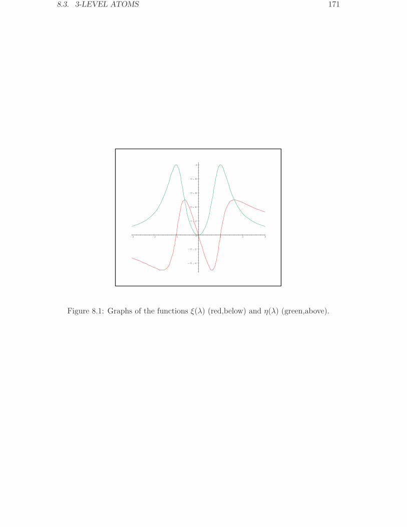
8.3. 3-LEVEL ATOMS 171
-0.4
-0.2
0
0.2
0.4
0.6
0.8
1
-3 -2 -1 1 2 3
Figure 8.1: Graphs of the functions ξ(λ) (red,below) and η(λ) (green,above).

172 CHAPTER 8. FEW-LEVEL ATOMIC SYSTEMS
Chapter 9
Cavity QED
The general idea for modeling the coupled system of an atom and radiation in ahigh Q cavity is the following:
• There are only a few resonant modes dominating the radiation in the cavity.Therefore, in a reasonable approximate description, all other modes of thequantized radiation field may be disregarded.
• There are only a few levels of the atom involved in the interaction with thecavity field. Therefore, in a reasonable approximate description, the internalstate space of the atom subsystem may be restricted to describe just theselevels.
9.1 The Jaynes-Cummings Model
In the simplest model of cavity QED the radiation field is restricted to a single,essentially monochromatic mode a and the atom is described as a two-level quantumsystem at some fixed position in the cavity.
9.1.1 Quantized Radiation Field for Selected Modes
Let a1, a2 , . . . be a maximal family of pairwise orthogonal modes. Then, by (1.37),
f jν (k) = [aj(k), a†ν ]− ∀ j ∈ 1, 2 , ν ∈ R , k ∈ R
3 . (9.1)
(1.61) together with (1.33) implies
E(+)a1,...,an
(x)def= PHa1,...,an
E(+)0 (x, 0) PHa1,...,an
=n∑
ν=1
E aν(x) aν ∀n ∈ N ,(9.2)
173
174 CHAPTER 9. CAVITY QED
where
E aν(x)def= −i (2π)− 3
2
õ0~c
2∑
j=1
∫c |k| ǫj(k) [aj(k), a†ν ]− eik·x
dVk√2 |k|
. (9.3)
(1.61) together with (1.53) implies
Ha1,...,andef= PHa1,...,an
Hfield PHa1,...,an
=n∑
ν,µ=1
hνµ a†ν aµ ∀n ∈ N ,
(9.4)
where
hνµdef=
2∑
j=1
∫~ c |k|
(f jν (k)
)∗f jµ(k) dVk
= (hν′ν)∗ ∀ ν, µ ∈ N .
(9.5)
(9.4) simplifies to
Ha1,...,an =n∑
ν=1
hνν a†ν aν
if the modes aν are non-overlapping , i.e. if
ν 6= µ =⇒ f jν (k) fjµ(k) = 0 ∀ j ∈ 1, 2 .
Remark: Note that restriction to the non-overlapping modes a1, . . . , ancan only be consistent if, e.g., the a†1 Ω, . . . , a
†nΩ have (sufficiently) sharp
energy. Actually for cavity modes this is only possible due to a changeof boundary conditions resulting in a change of the dynamics. Thusrestricting the Hamiltonian of the radiation field to some non-overlappingmodes is much more drastic than restricting the Hamiltonian of an atomto a few levels.
9.1.2 Interaction of the Two-Level System with the CavityField
Let the atom be localized at x = 0 . Then the electric field representation discussedin 7.1.2 suggests using1
Hcavdef=
(PHm
⊗ PHa
)(Hatom + Hfield − q x · E0(0, 0)
)(PHm
⊗ PHa
)
= Hm + Ha − q xm · Ea , (9.6)
Draft, November 5, 2011
1Recall the agreement made in 7.1.1.
9.1. THE JAYNES-CUMMINGS MODEL 175
where
Eadef= E
(+)a (0) +
(E
(+)a (0)
)†, xm
def= PHm
x PHm, (9.7)
as an approximate Hamiltonian for interacting system of the two-level atom and thequantized single-mode radiation field.
Remark: Note that in the electric field representation pcan is to beinterpreted as the (approximate) observable of the mechanical — ratherthan canonical — momentum of the atom’s electron! Correspondingly,Hatom is to be interpreted as the (approximate) observable of the internalenergy of the one-electron atom.
Assuming2
〈Ψν | xΨν〉 = 0 for ν = 1, 2 (9.8)
and defining
µ01def= q 〈Ψ0 | xΨ1〉 (9.9)
we getq xm = µ01 b+ µ∗
01 b† (9.10)
for the (restricted) atomic dipole operator in the matrix representation. This is asimple consequence of (9.7), (9.2), and (8.11). Moreover, defining
Edef= −i (2π)− 3
2
õ0~c
2∑
j=1
∫c |k| ǫj(k) [aj(k), a†ν ]−
dVk√2 |k|
we getEa = E a+ E
∗a† (9.11)
for the restricted electric field operator as a direct consequence of (9.7), (9.2), and(9.3).
Let us consider the special case3
µ01 = µme1 + i e2√
2, E = E0
e1 + i e2√2
. (9.12)
Then, up to an irrelevant additive constant, Hcav coincides with the Jaynes-Cummings
HamiltonianHJC
def= ~ω0 b
†b+ ~ω a†a+ λ a†b+ λ∗ a b† , (9.13)
Draft, November 5, 2011
2This assumption is usually fulfilled for the stationary states Ψ0,Ψ1 of the atom.3The first condition corresponds to Ψ1 → Ψ0 being a ∆m = ±1-transition. If the conditions
(9.12) are not fulfilled (9.13) is called rotating-wave approximation; see, e.g., (Schleich, 2001,Section 14.8.2).
176 CHAPTER 9. CAVITY QED
where
ωdef= ~
−1
2∑
j,j′=1
∫c |k| [a, a†j(k)]− [aj′(k), a
†]− dVk , λdef= µm E0 .
Proof: Thanks to
(e1 + i e2)2= 0 , (e1 + i e2) (e1 − i e2) = 2
we have
− q xm · Ea =(9.10)–(9.12)
(µm
e1 + i e2√2
b+ µ∗m
e1 − i e2√2
b†)
·(E0
e1 + i e2√2
a+ E∗0
e1 − i e2√2
a†)
= λ a†b+ λ∗ a b† . (9.14)
(9.2), (9.3), and (9.1) implyHa = ~ω a†a . (9.15)
(8.4) and (8.9), finally, imply
Hm − ~ω0 b†b ∝ 1 , (9.16)
Now, the statement is a direct consequence of (9.14)–(9.16).
Without loss of generality, we assume that4
λ = λ∗ .
WithH(0) def
= α |0, 0〉 : α ∈ Cand
H(n+1) def=
(α1
α0
)
n
def= α0 |0, n+ 1〉+ α1 |1, n〉 : α0, α1 ∈ C
∀n ∈ Z+ ,
where
|j, n〉 def= Ψj ⊗
1√n!
(a†)n
Ω ∀ j ∈ 0, 1 , n ∈ Z+ .
we have
Hm ⊗Ha =∞⊕
n=0
H(n)
and, obviously, HJC leaves all the H(n) invariant. For every n ∈ Z+ , since
a† |j, n〉 =√n+ 1 |j, n+ 1〉 , a |j, n+ 1〉 =
√n+ 1 |j, n〉 ,
Draft, November 5, 2011
4Otherwise we could change a by a phase factor to arrange this.
9.1. THE JAYNES-CUMMINGS MODEL 177
we have
HJC
(α1
α0
)
n
= H(n+1)JC
(α1
α0
)
n
∀α0, α1 ∈ C
with
H(n+1)JC
def=
(~ω0 + n ~ω λ
√n+ 1
λ√n+ 1 (n+ 1) ~ω
)
= En τ0 + λ
√n+ 1 τ 1 + ~
δ
2τ 3 (9.17)
andEn
def= ~
(ω0 + (n+ 1/2)ω
), δ
def= ω0 − ω (detuning) . (9.18)
In order to exploit (9.17), note that5
eiϕ·τ τ e−iϕ·τ = D2ϕ τ ∀ϕ ∈ R3 . (9.19)
Sketch of proof: A straightforward calculation using (8.8) shows that
f(ϕ) = f1(ϕ)def= ei ϕ e·τ τ e−i ϕ e·τ
is a solution of the initial value problem
d
dϕf(ϕ) = 2 e× f(ϕ) , f(0) = τ .
Since alsof(ϕ) = f2(ϕ)
def= D2ϕ e τ
is such a solution, both f1(ϕ) and f2(ϕ) must coincide.
Thuse+i
i~H
(n+1)JC t τ e−i
i~H
(n+1)JC t = D2Ωnt e′n τ , (9.20)
where
e′ndef=
√n+ 1λ/~
0δ/2
/Ωn
and
Ωndef=
√(λ
~
)2
(n+ 1) +
(δ
2
)2
(Rabi frequency) . (9.21)
Note that, according to (8.13), the nutation of the Bloch vector (relative to e3) cor-responds to transitions between the two levels of the atom with a circular frequencyΩn .
Draft, November 5, 2011
5By Dϕ we denote rotation around the axis along ϕ by the angle |ϕ| .
178 CHAPTER 9. CAVITY QED
Assume that
Ψ(n+1) =
(α1
α0
)
n
∈ H(n+1) , α1 ≥ 0 ,
is a normalized eigenstate of H(n+1)JC , n ∈ Z+ , Then, by (9.20),
α1 (α0 + α∗0)
−i α1 (α0 − α∗0)
|α1|2 − |α0|2
=
⟨Ψ(n+1) | τ Ψ(n+1)
⟩= σe′n
holds for either σ = +1 or σ = −1 . This implies σ α0 ≥ 0 and, together withnormalization:
(α1)2 + (α0)
2 = 1 , (α1)2 − (α0)
2 =σ δ
2Ωn
.
Thus,
α1 =+
√1
2+
σ δ
4Ωn
, α0 = σ +
√1
2− σ δ
4Ωn
holds for either σ = +1 or σ = −1 . We conclude thatΨ(n+1)σ
def= +
√1
2+
σ δ
4Ωn
|1, n〉+ σ +
√1
2− σ δ
4Ωn
|0, n+ 1〉 : σ ∈ −,+
is a maximal orthonormal set of eigenvectors of H(n+1)JC :
H(n+1)JC Ψ
(n+1)± =
(En ± ~Ωn
)Ψ
(n+1)± . (9.22)
Proof of (9.22): The statement is a direct consequence of
(H
(n+1)JC − En τ
0)(
α1
α0
)
n
=(9.17)
λ√n+ 1α0 + ~
δ
2α1
λ√n+ 1α1 − ~
δ
2α0
n
=(9.17)
(λ√n+ 1
α0
α1+ ~
δ
2
)α1
(λ√n+ 1
α1
α0− ~
δ
2
)α0
n
and
λ√n+ 1σ
√2Ωn ∓ σ δ
2Ωn ± σ δ± ~
δ
2=
σ λ√n+ 1 (2Ωn ∓ σ δ)√4 (Ωn)
2 − δ2± ~
δ
2
=(9.21)
σ λ√n+ 1 (2Ωn ∓ σ δ)
2 λ~
√n+ 1
± ~δ
2
= σ ~Ωn .
9.1. THE JAYNES-CUMMINGS MODEL 179
Sinceeiϕ·τ = cos |ϕ| τ 0 + i sin |ϕ| ϕ
|ϕ| · τ ∀ϕ ∈ R3
(see Exercise E25b) of (Lucke, eine)), (9.17) also implies
e−i~H
(n+1)JC t = e−
i~En t
(cos (Ωn t) τ
0 − i sin (Ωn t)
(λ√n+ 1
~Ωn
τ 1 +δ
2Ωn
τ 3))
.

180 CHAPTER 9. CAVITY QED
Appendix A
A.1 Functional Taylor Expansion
Of course, the polarization of a nonlinear medium should be a nonlinear func-tional of electromagnetic field. The first order functional derivative characterizesthis functional only approximately (fortunately with very high precision for usualfields). This is why a functional Taylor expansion is needed.
Let T be some complex vector space of functions on Rn with norm1 ‖.‖ and let
F be a continuous (complex) functional on T , i.e. a continuous mapping from Tinto C . Then the functional derivative2 of F at g ∈ T , if it exists, is the uniquebounded linear Functional Lg on T fulfilling
limǫ→+0
supϕ∈T‖ϕ‖<ǫ
1
ǫ|F (g + ϕ)− F (g)− Lg(ϕ)| = 0
and is identified with the generalized functionδ
δg(x)F (g) :
∫
Rn
(δ
δg(x)F (g)
)ϕ(x) dVx
def= Lg(ϕ) ∀ϕ ∈ T .
Note that∫
Rn
(δ
δg(x)F (g)
)ϕ(x) dVx = lim
ǫ→+0
F (g + ǫ ϕ)− F (g)
ǫ∀ϕ ∈ T
if Lg exists. More generally, the n-fold functional derivative
δ
δg(x1). . .
δ
δg(xν)F (g)
Draft, November 5, 2011
1The linear space T need not be complete w.r.t. ‖.‖ .2This is a special case of the Frechet derivative (see, e.g., (Choquet-Bruhat et al., 1978,
p. 71)).
181
182 APPENDIX A. APPENDIX
of F at g is iteratively defined by∫
R(ν+1)n
(δ
δg(x1). . .
δ
δg(xν+1)F (g)
)ϕ1(x1) . . . ϕν+1(xν+1) dVx1 . . . dVxν+1
def=
∫
Rn
(δ
δg(x)Fϕ2,...,ϕν+1(g)
)ϕ1(x) dVx ∀ϕ1, . . . , ϕν+1 ∈ T ,
where
Fϕ2,...,ϕν+1(g)
def=
∫
Rνn
(δ
δg(x2). . .
δ
δg(xν+1)F (g)
)ϕ2(x2) . . . ϕν+1(xν+1) dVx2 . . . dVxν+1
∀ϕ2, . . . , ϕν+1 ∈ T .
This amounts to∫
Rνn
(δ
δg(x1). . .
δ
δg(xν)F (g)
)ϕ1(x1) . . . ϕν(xν) dVx1 . . . dVxν
=
(∂
∂ǫ1. . .
∂
∂ǫνF (g + ǫ1 ϕ1 + . . . ǫν ϕν)
)
|ǫ1=...=ǫν=0
∀ϕ1, . . . , ϕν ∈ T(A.1)
wheneverδ
δg(x1). . .
δ
δg(xν)F (g) exists. (A.1) especially implies
((∂
∂ǫ
)νF (g + ǫ ϕ)
)
|ǫ=0
=
∫
Rνn
(δ
δg(x1). . .
δ
δg(xν)F (g)
)ϕ(x1) . . . ϕ(xν) dVx1 . . . dVxν
∀ϕ ∈ T .
Therefore, for sufficiently well-behaved F , we have the functional Taylor ex-pansion
F (ϕ) =(e∫dVx ϕ(x)
δδg(x)F (g)
)|g=0
def= F (0) +
∞∑
ν=1
1
ν!
∫Fν(x1, . . . ,xν)ϕ(x1) . . . ϕ(xν) dVx1 . . . dVxν
,
where
Fν(x1, . . . ,xν)def=
(δ
δg(x1). . .
δ
δg(xν)F (g)
)
|g=0
∀ ν ∈ N .
More precisely, we have
F (ϕ) = F (0) +
n∑
ν=1
1
ν!
∫Fν(x1, . . . ,xν)ϕ(x1) . . . ϕ(xν) dVx1
. . . dVxν
+1
n!
∫ 1
0
(1− λ)n
(d
dλ
)n+1
F (λϕ) dλ ,
This formalism has a straightforward generalization to vector-valued functions g onRn .
A.2. ELEMENTARY QUANTUM MECHANICS 183
A.2 Elementary Quantum Mechanics3
A.2.1 Scalar Particles in R1
(In the Schrodinger picture) the (pure) state of a single, free, 1-dimensional,scalar, quantummechanical ‘particle’ of massm is always given by awave functionΨ(x, t) fulfilling the free Schrodinger equation
i∂
∂tΨ(x, t) =
Hkindef=︷ ︸︸ ︷
1
2mp2 Ψ(x, t) , (A.2)
where
pdef=
~
i
∂
∂x. (A.3)
Its basic interpretation is
∫
G|Ψ(x, t)|2 dx = probability for ‘position at time t inside G’ (A.4)
for all (sufficiently well-behaved) region G ⊂ R and requires4
∫|Ψ(x, t)|2 dx = 1 (A.5)
for all t ∈ R . Simple asymptotic considerations5 show that the spatial Fouriertransform
Ψ(p, t)def=
1√2π~
∫Ψ(x, t) e
i~p xdx (A.6)
(adapted to quantum mechanics) has a similar interpretation w.r.t. linear momen-tum:6
∫
G
∣∣∣Ψ(p, t)∣∣∣2
dp = probability for ‘momentum at time t inside G’. (A.7)
The latter is consistent in the sense that∫ ∣∣∣Ψ(p, t)
∣∣∣2
dp =
∫|Ψ(x, t)|2 dx (A.8)
= 1 .Draft, November 5, 2011
3For mathematical details see, e.g., (Lucke, fuan).4As usual, we write
∫for∫∞
−∞ resp.∫R. One can easily show that (A.2) guarantees that (A.5)
holds for all t if fulfilled for t = 0 .5See, e.g., (Lucke, 1995, Section 5).6Actually, (A.2) implies the l.h.s. of (A.7) — contrary to the l.h.s. of (A.4) — to be independent
of t .
184 APPENDIX A. APPENDIX
Defining
Ψt(x)def= Ψ(x, t) ,
〈Ψ | Φ〉 def=
∫Ψ(x)Φ(x) dx ,
and the position observable x by
(xΨ) (x)def= xΨ(x) (A.9)
one gets
〈Ψt | xΨt〉 =∫x |Ψt(x)|2 dx
and hence7
〈Ψt | xΨt〉 = 〈x(t)〉 def=
expectation value for the position variablex at time t in the state given by Ψt .
(A.10)
Similarly one has
〈Ψt | pΨt〉 = 〈p(t)〉 def=
expectation value for the momentum variablep at time t in the state given by Ψt ,
(A.11)
sinceΦ(x, t) = pΨ(x, t) =⇒ Φ(p, t) = p Ψ(x, t)
and, therefore, the generalization
∫Φ(x)Ψ(x) dx =
∫Φ(p) Ψ(p) dp (A.12)
of (A.8) implies
〈Ψt | pΨt〉 =∫p∣∣∣Ψ(p, t)
∣∣∣2
dp . (A.13)
In view of (A.11), p is called momentum observable . (A.10) and (A.11) areconsistent in the sense that
(A.2) =⇒ d
dt〈x(t)〉 = 1
m〈p(t)〉 = constant. (A.14)
Similarly to (A.14) one gets
〈Ψt | Hkin︸︷︷︸= p2
2m=− ~2
2m(∂∂x)
2
Ψt〉 =∫
p2
2m
∣∣∣Ψ(p, t)∣∣∣2
dp
Draft, November 5, 2011
7Note, however, that 〈x(t)〉 may be infinite.
A.2. ELEMENTARY QUANTUM MECHANICS 185
and, therefore,⟨Ψt
∣∣∣ p2
2mΨt
⟩= 〈Ekin(t)〉 def
=
expectation value for the kinetic energyat time t in the state given by Ψt .
(A.15)
If the particle is not free but interacting with an external force field with poten-tial8 V (x) then, of course, (A.2) has to be modified. The basic interpretations (A.4)and (A.7), however, are maintained. Therefore, also (A.10) resp. (A.11) has to bemaintained for (A.9) resp. (A.3). But now, in addition, we have
〈Ψt | V (x)Ψt〉 = 〈Ekin(t)〉 def=
expectation value for the potential energyat time t in the state given by Ψt .
(A.16)Assuming that the expectation value of the total energy is the sum of the expectationvalues for kinetic and potential energy, one concludes from (A.15) and (A.16) that
⟨Ψt | H Ψt
⟩= 〈E(t)〉 def
=
expectation value for the total energyat time t in the state given by Ψt ,
(A.17)
where the operator
Hdef=
p2
2m+ V (x) (Hamiltonian) (A.18)
is the observable for the total energy. The latter suggests replacing (A.2) by thetime dependent Schrodinger equation
i∂
∂tΨ(x, t) = H Ψ(x, t) , (A.19)
coinciding with (A.2) for V = 0 . This is consistent in the sense that — generalizing(A.14) — (A.19) implies the Ehrenfest equations
d
dt〈x(t)〉 = 1
m〈p(t)〉 , d
dt〈p(t)〉 =
∫ (− d
dxV (x)
)|Ψ(x, t)|2 dx
and 〈E(t)〉 =constant.
A.2.2 Energy Eigenstates of the Harmonic Oscillator
One of the main objectives of quantum mechanics is to determine the (possiblyimproper) energy eigenfunctions, i.e. those Ψ(x) for which there is an energy valueE with
H Φ(x) = EΨ(x) . (A.20)
Draft, November 5, 2011
8For particles interacting with a general electromagnetic field see 7.1.1.
186 APPENDIX A. APPENDIX
These eigenfunctions give rise to the special solutions
Ψ(x, t) = e−i~E tΨ(x) (A.21)
of (A.19) called stationary , since
(A.21) =⇒ ∂
∂t|Ψ(x, t)|2 = 0 .
Let us solve (A.20) for the (quantum mechanical) harmonic oscillator ,characterized by
V (x) =m
2ω2 x2 . (A.22)
This problem is easily solvable by means of the operators
adef=
p− imω x√2m ~ω
, a†def=
p+ imω x√2m ~ω
(A.23)
fulfilling the commutation relations9
[a, a†
]− = 1 (A.24)
and hence the equations(a†a)a = a (a†a− 1) ,(
a†a)a† = a†(a†a+ 1) .
Iterating these equations gives10
(a†a)aν = aν
(a†a− ν
)∀ ν ∈ N , (A.25)
(a†a)(a†)ν
=(a†)ν (
a†a+ ν)
∀ ν ∈ N . (A.26)
Since
H =~
2ω(a† a+ a a†
)
= ~ω
(a† a+
1
2
), (A.27)
we have
H Ψ = EΨ =⇒
H (aν Ψ) =(A.25)
(E − ν) aν Ψ
H((a†)ν Ψ
)=
(A.26)(E + ν) (a†)ν Ψ
Draft, November 5, 2011
9We simply write z for z1 (with z ∈ C) in the following. Note that, in this sense, [p , x] = ~
i .10Note that, e.g., (A.26) also follows from
a(a†)ν
=(1.82)
(a†)νa+ ν
(a†)ν−1
.
A.2. ELEMENTARY QUANTUM MECHANICS 187
for all (sufficiently well-behaved) Ψ . Thus, if Ψ is an eigenfunction of H witheigenvalue E then
⟨aν Ψ | H aν Ψ
⟩= (E − ν) 〈aν Ψ | aν Ψ〉
could become negative if aν Ψ were nontrivial for all ν ∈ N . The latter, however isimpossible because of
⟨Φ | H Φ
⟩=
(A.27)~ω 〈aΦ | aΦ〉+ 1
2~ω 〈Φ | Φ〉
> 0 ∀Φ 6= 0 .
Therefore:
For every eigenfunction Ψ of H there is some µ ∈ Z+ with
a (aµΨ) = 0 . (A.28)
Now, aµΨ is fixed — up to some factor — by (A.28):
a (aµΨ) = 0 =⇒(A.23),(A.3)
d
dx(aµΨ) (x) = −mω
~x (aµΨ) (x)
=⇒ d
dxln (aµΨ) (x) = −mω
~x
=⇒ (aµΨ) (x) ∼ e−mω2 ~
x2 .
We conclude that
H Ψ = EΨ =⇒ 0 6= aµΨ ∼ Ω for some µ ∈ Z+ , (A.29)
where11
Ω(x)def=(mω
π ~
) 14e−
mω2 ~
x2 , aΩ = 0 . (A.30)
Iterating (a†)νaν =
(a†)ν−1 (
a†a)aν−1
=(A.25)
(a†)ν−1
aν−1(a†a− (ν − 1)
)
we get (a†)νaν =
(a†a)(a†a− 1
)· · ·(a†a− (ν − 1)
)∀ ν ∈ N (A.31)
and conclude:12
H(a†)µ
Ω =(A.26),(A.30)
(µ+
1
2
)~ωΩ ∀µ ∈ Z+ ,
Draft, November 5, 2011
11Note that
∫e−x
2
dx =√π
(more generally, see (2.83)
), hence 〈Ω | Ω〉 = 1 .
12Note thataµΨ 6= 0 =⇒
(a†)µaµΨ 6= 0 ,
188 APPENDIX A. APPENDIX
H Ψ = EΨ =⇒(A.29),(A.31),(A.27)
Ψ ∼(a†)µ
Ω for some µ ∈ Z+ ,
A.2.3 Coherent States
Recall13 that the operators
aoscdef=
~
iddx
− imω x√2m ~ω
, a†osc =~
iddx
+ imω x√2m ~ω
of the 1-dimensional harmonic oscillator with Hamiltonian
Hoscdef= − ~
2
2m
(d
dx
)2
+1
2mω2 x2
also obey the commutation relation
[aosc, a
†osc
]− = 1
and that
Hosc =~
2ω(a†osc aosc + aosc a
†osc
),
hence
Hosc = ~ω
(a†osc aosc +
1
2
).
Here the ground state
Ωosc(x)def=(mω
π ~
) 14e−
mω2 ~
x2
corresponds to the vacuum:aosc Ωosc = 0 .
Therefore, since
α a†osc − α aosc = ℑ(α)√
2 ~
mω
d
dx+ iℜ(α)
√2mω
~x ,
the corresponding coherent states, according to (1.79) and (1.74), are
Ψaosc,α(x) =(mω
π ~
) 14eiℜ(α)ℑ(α) eiℜ(α)
√2mω
~x e
− mω2 ~
(x+ℑ(α)
√2 ~
mω
)2.
This shows that the coherent states of the harmonic oscillator are just displace-ments in position and momentum of the ground state, hence have the same minimal
Draft, November 5, 2011
13See A.2.2.
A.3. CONSTRUCTION OF FIELD OPERATORS 189
uncertainty product14
∆x∆p =~
2=
~
2∆(a+ a†)∆(i a− i a†) .
In this sense, the coherent states of the quantized electromagnetic field correspondto coherent classical fields as closely as possible.15
A.3 Construction of Field Operators
Denote by F the complex vector space of all truncated sequences
f = f0, f1, f2, . . .
of (sufficiently well-behaved) functions16 fν(k1, j1; . . . ;kν , jν) over (R3 × 1, 2, 3)νfulfilling17
fν(kπ1, jπ1; . . . ;kπν , jπν) = fν(k1, j1; . . . ;kν , jν) ∀ π ∈ Sν
and3∑
j1,...,jν=1
∫|fν(k1, j1; . . . ;kν , jν)|2 dVk1 . . . dVkν
<∞ .
Of course, the linear structure is meant to be the natural one:
z f = z f0, z f1, z f2, . . . ∀ z ∈ C , f ∈ F ,
f+ f′def= f0 + f ′
0, f1 + f ′1, f2 + f ′
2, . . . ∀ f, f′ ∈ F .
With the inner product
〈f | f′〉 def= f0 f
′0 +
3∑
j1,...,jν=1
∫fν(k1, j1; . . . ;kν , jν) f
′ν(k1, j1; . . . ;kν , jν)dVk1 . . . dVkν
Draft, November 5, 2011
14Quite generally we have
∥∥∥(A− a)Ψ∥∥∥2 ∥∥∥(B − b)Ψ
∥∥∥2
≥∣∣∣⟨(A− a
)Ψ∣∣∣(B − b
)Ψ⟩∣∣∣
2
= 14
∥∥∥∥⟨Ψ∣∣∣ [A, B]− Ψ
⟩
︸ ︷︷ ︸real
∥∥∥∥2
+ 14
∥∥∥∥⟨Ψ∣∣∣ [A− a, B − b]+ Ψ
⟩
︸ ︷︷ ︸imaginary
∥∥∥∥2
.
for all selfadjoint operators A, B , all real numbers a, b , and every vector Ψ ∈ DBA ∩DAB .15States with ∆(a + a†) < 1 or ∆(i a − i a†) < 1 are called squeezed states (see
(Scully and Zubairy, 1999, Sections 2.5–2.8) for a discussion of these states).16The physical dimension of the values of these functions should be such that the integrals∫|fν(k1, j1; . . . ;kν , jν)|2 dVk1
. . . dVkνare just real numbers without any physical dimension.
17As usual, we denote by Sν the group of all permutations of (1, . . . , ν) .
190 APPENDIX A. APPENDIX
F becomes a euklidean vector space (pre-Hilbert space). Now let us introduceoperator-valued functions bj(k) by
18
f− = bj(k) f
def⇐⇒ f−ν (k1, j1; . . . ;kν , jν) = ℓ−
32√ν fν+1(k1, j1; . . . ;kν , jν ;k, j) ∀ ν ∈ Z+ ,
where ℓ is some fixed length necessary for adjusting the physical dimensions. Then
for the adjoint operators(bj(k)
)†, characterized by
⟨f∣∣∣ bj(k) f′
⟩=
⟨(bj(k)
)†f∣∣∣ f′⟩
∀ f, f′ ∈ F ,
we have f+ =(bj(k)
)†f iff f+
0 = 0 and:
ℓ32 f+
ν+1(k1, j1; . . . ;kν+1, jν+1)
=1√ν + 1
ν∑
µ=1
δjnuj δ (kµ − k) fν+1(k1, j1; . . . ;kµ\, jµ\; . . . ;kν+1, jν+1) ∀ ν ∈ Z+ .
Consequently, we have the commutation relations
[bj(k), bj′(k′)]− = 0 ,
[bj(k),
(bj′(k
′))†]
−= ℓ−3 δjj′ δ(k− k′)
and the definition
aj(k)def= ℓ
32 ǫj(k) · b(k) ∀ j ∈ 1, 2 , k ∈ R
3 ,
where
b(k)def=
3∑
j=1
bj(k) ej ,
yields a realization of the canonical commutation relations (1.37) fulfilling (1.38) for
Ωdef= (1, 0, 0, . . .) .
Note that2∑
j=1
ǫj(k) aj(k) = b(k)− k
|k| · b(k) ∀k 6= 0 .
This shows that A(+)(x, t) does not depend on the choice of polarization vectorsǫj(k) in (1.31).
Draft, November 5, 2011
18Of course ‘. . . ;kν , jν ’ should be dropped for ν ≤ 1 and also ‘k1, j1’ if ν = 0 .
A.4. DYSON SERIES 191
A.4 Dyson Series
In the Schrodinger picture the state vectors (wave functions) Ψt = ΨSt de-
scribe the momentary situation of the quantum system at time t . Thus, if A = AS
is the observable of a physical quantity A then⟨ΨSt | ASΨS
t
⟩is the correspond-
ing expectation value for A at time t . The time evolution is described by theSchrodinger equation
i~∂
∂tΨSt = HS(t)ΨS
t . (A.32)
Now assume that the Hamiltonian in the Schrodinger picture is of the form
HS(t) = HS0 + V S(t) , (A.33)
Where HS0 (t) corresponds to some known ‘free evolution’ and V S(t) is some pertur-
bation of the ‘free’ Hamiltonian HS0 (t) . Then we may get a perturbative solution
of (A.32) by switching to the interaction picture:19
ΨSt 7−→ ΨI
tdef= e
i~HS0 tΨS
t , (A.34)
AS(t) 7−→ AI(t)def= e+
i~HS0 tAS(t) e−
i~HS0 t . (A.35)
This way (A.32) becomes equivalent to
i~∂
∂tΨIt = V I(t)ΨI
t . (A.36)
Sure, (A.36) has the same formal structure as (A.32). Now, however, for the suffi-ciently small T the mapping20
I : Φ(t) 7−→ − i
~
∫ t
0
V I(t) Φ(t′) dt′ (A.37)
may be contracting with respect to the norm
‖Φ‖Tdef=
∫ T
0
‖Φ(t)‖ dt ;
i.e. the may be some λ < 1 with
‖Φ‖T ≤ λ ‖Φ‖T ∀Φ .If this is the case we have
ΨIt =
∞∑
ν=0
(IνΨI
0
)(t) ∀ t ∈ [0, T ] (A.38)
Draft, November 5, 2011
19See (Lucke, qft, Sect. 3.1.3) for a qualitative discussion.20Here we assume that Φ(t) is a (sufficiently well behaved) function of t with values in the state
space H and denote by ‖.‖ the norm corresponding to the inner product of H .
192 APPENDIX A. APPENDIX
(compare Section 5.1.3 of (Lucke, ein)), since (A.36) is equivalent to the integralequation
ΨIt = ΨI
0 −i
~
∫ t
0
V I(t′)ΨIt′ dt
′ .
Using time ordering21
T(V I(tπ1) · · · V I(tπν)
)def= V I(t1) · · · V I(tν) ∀ t1 ≤ . . . ≤ tν , π ∈ Sν
we may rewrite (A.38) as Dyson series :22
ΨIt = T
(e−
i~
∫ t0 V
I(t′) dt′)ΨI
0
def= ΨI
0(0) +∞∑
ν=1
1
ν!
(− i
~
)ν ∫
[0,t]νT(V I(t1) · · · V I(tν)
)ΨI
0 dt1 · · · dtν .
(A.39)Usually only the first order approximation
ΨIt ≈ ΨI
0 −i
~
∫ t
0
V I(t′)ΨI0 dt
′ ∀ t ∈ [0, T ] (A.40)
is used — as justified for sufficiently small T . This implies for the transitionprobability
∣∣⟨Φ00 | ΨI
t
⟩∣∣ ≈ ~−2
∣∣∣∣∫ t
0
⟨Φ0
0 | V I(t′)ΨI0
⟩dt′∣∣∣∣2
if⟨Φ0
0 | ΨIt
⟩= 0 . (A.41)
Remark: Since
∣∣∣∣∫ t
0
⟨Φ0
0 | V I(t′)ΨI0
⟩dt′∣∣∣∣2
=
∫
[0,t]×[0,t]
⟨Φ0
0 | V I(t1)ΨI0
⟩⟨ΨI
0 | V I(t2) Φ00
⟩dt1 dt2 ,
the corresponding formula for mixed states with density matrix ρIt is
trace(ρIt∣∣Φ0
0
⟩⟨Φ0
0
∣∣)≈ ~
−2
∫
[0,t]×[0,t]
⟨Φ0
0 | V I(t1) ρI0 V
I(t2) Φ00
⟩dt1 dt2 ,
in agreement with (6.19).
Draft, November 5, 2011
21As usual, we denote by Sν the set of all permutations of 1, . . . , ν .22Of course, we tacitly assume also t 7→ V I(t) to be sufficiently well behaved.
Bibliography
Abramsky, S. and Coecke, B. (2004). A categorical semantics of quantum protocols.quant-ph/0402130, pages 1–16. 118
Agranovich, V. M. and Ginzburg, V. L. (1984). Crystal Optics with Spatial Disper-sion and Excitons, volume 42 of Solid-State Sci. Springer-Verlag, 2. edition.36
Agrawal, G. P. (1999). Nonlinear fiber optics. Optics and Photonics. AcademicPress. 61
Alicki, R. (2003). Controlled quantum open systems. Lecture Notes in Physics,622:121–139. quant-ph/0302132. 137
Alleaume, R., Treussart, F., Courty, J.-M., and Roch, J.-F. (2003). Photon statisticscharacterization of a single photon source. quant-ph/0312084, pages 1–22. 114
Angelo, R. M. and Wreszinski, W. F. (2005). Quantum NOT operation and inte-grability in two-level systems. quant-ph/0502102, pages 1–17. 159
Armstrong, J., Bloembergen, N., Ducuing, J., and Pershan, P. S. (1962a). Interac-tions between light waves in a nonlinear dielectric. Phys. Rev., 127:1918–1939.63
Armstrong, J. A., Bloembergen, N., Ducuing, J., and Pershan, P. S. (1962b). Inter-actions between light waves in a nonlinear dielectric. Phys. Rev., 127:1918–1939.72, 76
Aspect, A. (2004). Bell’s theorem : The naive view of an experimentalist.quant-ph/0402001, pages 1–34. 116
Azzam, R. M. A. and Bashara, N. M. (1987). Ellipsometry and Polarized Light.Elsevier Science B.V. 44
Bachor, H.-A. (1998). A Guide to Experiments in Quantum Optics. Wiley-VCH. 3
Baym, G. (1969). Lectures on Quantum Mechanics. Benjamin, New York. 147
193
194 Bibliography
Bennet, C. H. and Brassard, G. (1984). Quantum cryptography, public key distribu-tion and coin tossing. In Proceedings of International Conference on ComputerSystems and Signal Processing, pages 175–179, New York. IEEE. 113
Bloembergen, N. (1996a). Encounters in Nonlinear Optics, volume 16 of WorldScientific Series in 20th Century Physics. World Scientific.
Bloembergen, N. (1996b). Nonlinear Optics. World Scientific. 10, 43
Borchers, H.-J. (1990). Eine Bemerkung zur Ausbreitung von Licht in dis-pergierenden Medien. In Nachrichten der Akademie der Wissenschaften inGottingen aus dem Jahre 1990, pages 1–8. Vandenhoeck & Ruprecht, Gottingen.Mathematisch-Physikalische Klasse. 41
Bowmeester, D., Howell, J. C., and Lamas-Linares, A. (2002). Quantum informationscience using photons. Lecture Notes in Physics, 587:149–197. 106
Bowmeester, D., Pan, J., Mattle, K., Eibl, M., Weinfurter, H., and Zeilinger, A.(1997). Experimental quantum teleportation. Nature, 390:575–579. 108
Brukner, C. and Zeilinger, A. (2002). Young’s experiment and the finiteness ofinformation. Phil. Trans. R. Soc. Lond. A, 360:1061. quant-ph/0201026. 86
Brunner, W. and Junge, K. (1982). Lasertechnik. Dr. Alfred Huthig Verlag, Heidel-berg. 63
Busch, P., Grabowski, M., and Lahti, P. J. (1995). Operational Quantum Physics,volume m 31 of Lecture Notes in Physics. Springer-Verlag. 128
Carmichael, H. (1993). An Open Systems Approach to Quantum Optics, volume m18 of Lecture Notes in Physics. Springer-Verlag. 137
Carmichael, H. J. (2001). Quantum fluctuations of light: A modern perspective onwave/particle duality. quant-ph/0104073. 102
Caves, C. M., Fuchs, C. A., and Schack, R. (2002). Unknown quantum states:The quantum de Finetti representation. J. Math. Phys., 43:4537–4559.quant-ph/0104088. 108
Chen, Q.-H., Liu, T., Zhang, Y.-Y., and Wang, K.-L. (2010). Solutionsto the Jaynes-Cummings model without the rotating-wave approximation.arXiv:1011.3280 [quant-ph], pages 1–6. 159
Choquet-Bruhat, Y., Dewitt-Morette, C., and Dillard-Bleick, M. (1978). Analysis,Manifolds and Physics. North-Holland Publishing Company. 181
Coecke, B. (2004). The logic of entanglement. quant-ph/0402014, pages 1–8. 118
Bibliography 195
Cohen-Tannoudji, C., Dupont-Roc, J., and Grynberg, G. (1992). Atom-PhotonInteractions. John Wiley & Sons, Inc. 142
Davies, E. B. (1976). Quantum Theory of Open Systems. Academic Press. 128, 137
Deutsch, D. (1997). The Fabric of Reality. Penguin Books. 139
Di Giuseppe, G., Atature, M., Shaw, M. D., Sergienko, A. V., Saleh, B. E. A.,Teich, M. C., Miller, A. J., Nam, S. W., and Martinis, J. (2003). Observationof bosonic coalescence of photon pairs. quant-ph/0306131, pages 1–4. 107
Dowling, J. P., Franson, J. D., Lee, H., and Milburn, G. J. (2004). Towards linearoptical quantum computers. quant-ph/0402090, pages 1–9. 126
Duan, L.-M., Lukin, M. D., Cirac, J. I., and Zoller, P. (2001). Long-distance quan-tum communication with atomic ensembles and linear optics. Nature, 414:413–418. quant-ph/0105105. 119
Elitzur, A. and Vaidman, L. (1993). Quantum-mechanical interaction-free measure-ments. Found. Phys., 23:987–997. 110
Ficek, Z. and Swain, S. (2001). Quantum interference in optical fields and atomicradiation. quant-ph/0109100, pages 1–30. 86, 87
Fleischhauer, M. and Lukin, M. D. (2000). Dark-state polaritons in electromag-netically induced transparency. Phys. Rev. Lett., 84:5094. quant-ph/0001094.163
Fleischhauer, M. and Lukin, M. D. (2002). Quantum memory for photons: Dark-state polaritons. Phys. Rev. Lett., 65:022314. 122
Fredenhagen, K. (Winter Term 2000/2001). Quantenfeldthe-orie. Notes from lectures held at Hamburg University,http://unith.desy.de/research/aqft/lecture_notes. 16
Frohlich, J. (1977). Application of commutator theorems to the integration of repre-sentations of Lie algebras and commutation relations. Commun. Math. Phys.,54:135–150. 26
Frohlich, J., Griesemer, M., and Schlein, B. (2003). Asymptotic completeness forCompton scattering. mp arc/03-504, pages 1–63. 140
Gardiner, C. W. and Zoller, P. (2000). Quantum Noise, volume 56 of SpringerSeries in Synergetics. Springer, 2. edition. A Handbook of Markovian andNon-Markovian Quantum Stochastic Methods with Applications to QuantumOptics.
196 Bibliography
Garrison, J. C. and Chiao, R. Y. (2004). Canonical and kinetic forms of the elec-tromagnetic momentum in an ad hoc quantization scheme for a dispersive di-electric. quant-ph/0406222. 78
Gatti, A., Zambrini, R., Miguel, M. S., and Lugiato, L. A. (2003). Multi-photon, multi-mode polarization entanglement in parametric down-conversion.quant-ph/0306133, pages 1–22. 112
Gemmer, J. and Mahler, G. (2001). Entanglement and the factorization-approximation. Eur. Phys J. D, 17:385–393. quant-ph/0109140. 142
Gerhardt, I., Liu, Q., Lamas-Linares, A., Skaar, J., Scarani, V., Makarov, V., andKurtsiefer, C. (2011). Experimentally faking the violation of bell’s inequalities.arXiv:1106.3224 [quant-ph], pages 1–5. 116
Gingrich, R. M., Ko, P., Lee, H., Vatan, F., and Dowling, J. P. (2003). An all linearoptical quantum memory based on quantum error correction. Phys. Rev. Lett.,91:217901. quant-ph/0306098. 119
Gisin, N. and Gisin, B. (1999). A local hidden variable model of quantum correlationexploiting the detection. Phys. Lett. A, 260:323–327. quant-ph/9905018. 116
Gisin, N., Marcikic, I., de Riedmatten, H., Tittel, W., and Zbinden, H. (2003). Quan-tum communications with time-bin entangled photons: long distance quantumteleportation and quantum repeaters. quant-ph/0301181, pages 1–4. 108
Gjurchinovski, A. (2002). Polarization measurements - a numerical approach. Phys-ica Macedonica, 52:69–76. physics/0401105. 44
Gomez-Reino, C., Perez, M. V., and Bao, C. (2002). Gradient-Index Optics.Springer. Fundamentals and Applications. 57
Gottesman, D. and Chuang, I. L. (1999). Demonstrating the viability of universalquantum computation using teleportation and single-qubit operations. Nature,402:390–393. quant-ph/9908010. 126
Green, H. S. (1953). A general method of field quantization. Phys. Rev., 90:270–273.20
Grigorenko, A. N. (2006). Negative refractive index in artificial metamaterials.Optics Letters, 31:2483–2485. physics/0603216. 44
Hariharan, P. and Sanders, B. C. (1996). Quantum phenomena in optical interfer-ometry. Progress in Optics, 36:49–128. 87
Hentschel, M. and Schomerus, H. (2002). Fresnel laws at curved dielectric interfacesof microresonators. Phys. Rev. E, 65:045603(R). physics/0111160. 44
Bibliography 197
Hentschel, M. and Schomerus, H. (2006). Correcting ray optics at curved dielectricmicroresonator interfaces: Phase-space unification of Fresnel filtering and theGoos-Haenchen shift. Phys. Rev. Lett., 96:243903. physics/0606024. 44
Herbert, N. (1982). FLASH—A superluminal communicator based upon a new kindof quantum measurement. Foundations of Physics, 12:1171–1181. 112
Hodgson, J. N. (1970). Optical Absorption and Dispersion in Solids. Chapman andHall Ltd.
Hoffmann, F. (1994). Zur Strahlungstheorie wasserstoffahnlicher Atome unterBerucksichtigung der Schwerpunktsbewegung. Master’s thesis, Intitut fur Ma-thematische Physik, Technische Universitat Braunschweig. 140
Jackson, D. J. and Hockney, G. M. (2004). Detector efficiency limits on quantumimprovement. quant-ph/0402201, pages 1–7. 83
Jackson, J. D. (1975). Classical Electrodynamics, Second Edition. John Wiley &Sons, Inc., New York·London·Sydney. 44
Johansen, L. M. (2004). Nonclassicality of thermal radiation. J. Opt. B: QuantumSemiclass. Opt., 6:L21–L24. quant-ph/0402105. 99
Jones, R. C. (1941). New calculus for the treatment of optical systems. J. Opt. Soc.Am., 31:488. 44
Juzeliunas, G., Masalas, M., and Fleischhauer, M. (2003). Storing and releasinglight in a gas of moving atoms. Phys. Rev. A, page 023809. quant-ph/0210123.122
Kaltenbaek, R., Aspelmeyer, M., Jennewein, T., Brukner, C., Pfennigbauer, M.,Leeb, W. R., and Zeilinger, A. (2003). Proof-of-concept experiments for quan-tum physics in space. quant-ph/0308174, pages 1–15. 116
Kemble, E. C. (1937). The Fundamental Principles of Quantum Mechanics withElementary Applications. Dover Publications, Inc., New York. 127
Kim, Y.-H. and Grice, W. P. (2003). Quantum interference with distinguishablephotons through indistinguishable pathways. quant-ph/0304086, pages 1–6.107
Kim, Y.-H., Kulik, S. P., and Shih, Y. (2001). Quantum teleportation with a com-plete Bell state measurement. Phys. Rev. Lett., 86:1370. quant-ph/0010046.119
Kinsler, P., Favaro, A., and McCall, M. W. (2009). Four poynting theorems. Eur.J. Phys., 30:983. arXiv:0908.1721 [physics.optics]. 11
198 Bibliography
Klauder, J. R. (2010). On the role of coherent states in quantum foundations.arXiv:1008.4307 [quant-ph], pages 1–9. 24
Klauder, J. R. and Sudarshan, E. C. G. (1968). Fundamentals of Quantum Optics.W. A. Benjamin, Inc. 34, 85, 87, 89
Klein, A. (1999). Localization of light in randomized periodic media. In Fouque, J.-P., editor, Diffuse Waves in Complex Media, pages 73–92. Kluwer, The Nether-lands.
Kliger, D. S., Lewis, J. W., and Randall, C. E. (1990). Polarized Light in Opticsand Spectroscopy. Academic Press, Inc. 44
Klyshko, D. N. (1988). Photons and Nonlinear Optics. Gordon and Breach SciencePublishers.
Knill, E., Laflamme, R., and Milburn, G. (2000). Efficient linear optics quantumcomputation. Nature, 409:46. quant-ph/0006088. 126
Knill, E., Laflamme, R., and Milburn, G. J. (2001). A scheme for efficient quantumcomputation with linear optics. Nature, 409:46–52. 126
Kraus, K. (1983). Sates, Effects, and Operations, volume 190 of Lecture Notes inPhysics. Springer-Verlag. 128, 137
Kuang, L.-M., Chen, G.-H., and Wu, Y.-S. (2003). Nonlinear optical propertiesof an electromagnetically-induced transparency medium interacting with twoquantized fields. J. Optics B, 5:341–448. quant-ph/0402041. 163
Kuklinski, J. R., Gaubatz, U., Hioe, F. T., and Bergmann, K. (1989). Adiabaticpopulation transfer in a three-level system driven by delayed laser pulses. Phys.Rev. A, 40:6741–6744. 163
Kurtsiefer, C., Mayer, S., Zarda, P., and Weinfurther, H. (2000). A stable solid-statesource of single photons. Phys. Rev. Lett., 85:290. 101
Kwiat, P. G., Weinfurther, H., Herzog, T., Zeilinger, A., and Kasevich, M. A. (1995).Interaction-free measurement. Phys. Rev. Lett., 74:4763–4766. 110
Kwiat, P. G., White, A. G., Mitchell, J. R., Nairz, O., Weihs, G., Weinfurter, H., andZeilinger, A. (1999). High-efficiency quantum interrogation measurements viathe quantum Zeno effect. Phys. Rev. Lett., pages 4725–4728. quant-ph/9909083.110
Lamb, Jr., W. E. (1995). Anti-photon. Appl. Phys. B, pages 77–84. 13
Landau, L. and Lifschitz, E. (1967). Elektrodynamik der Kontinua, volume VIII ofLehrbuch der Theoretischen Physik. Akademie-Verlag, Berlin. 10, 12, 21
Bibliography 199
Leggett, A. J. (2001). Qubits, cbits, decoherence, quantum measurement and en-vironment. In Fundamentals of Quantum Information, pages 3–45. Springer.127, 156
Leonhardt, U. (2003). Quantum physics of simple optical instruments. Rept. Prog.Phys, 66:1207–1250. quant-ph/0305007. 102
Lewis, G. N. (1926). The conservation of photons. Nature, pages 874–875. 13
Lim, Y. L. and Beige, A. (2005). Generalised Hong-Ou-Mandel experiments withbosons and fermions. New J. Phys., 7:155. quant-ph/0505034. 107
Liu, C., Dutton, Z., Behroozi, C. H., and Vestergaard Hau, L. (2001). Observationof coherent optical information storage in an atomic medium using halted lightpulses. Nature, 409:490–493. 122
Lodenquai, J. (1991). Electromagnetic wave propagation in media with complexrefractive indices and transmission through absorbing films. Am. J. Phys.,59:248–254. 49
Loudon, R. (2000). The Quantum Theory of Light. Oxford Science Publications,third edition. 3, 24
Lucke, W. (1995a). Nonlinear Schrodinger dynamics and nonlinear observables.In Doebner, H.-D., Dobrev, V. K., and Nattermann, P., editors, Nonlinear,Deformed and Irreversible Quantum Systems, pages 140–154. World Scientific.183
Lucke, W. (1995b). Solutions of the inhomogeneous wave equation with unusualpropagation character and global solution of the Poisson equation. J. Phys. A,28:5393–5400. 10
Lucke, W. (1996). Axiomatic quantum theory. Acta Phys. Pol., 27:2357–2385. 130
Lucke, W. (edyn). Elektrodynamik .http://www.wolfgang-luecke.de/skripten/edyn.pdf. 9, 10, 25
Lucke, W. (ein). Mathematische Methoden der Physik.http://www.wolfgang-luecke.de/skripten/ein.pdf. 14, 19, 36, 65, 165,192
Lucke, W. (eine). Erganzungen zu “Mathematische Methoden der Physik”.http://www.wolfgang-luecke.de/skripten/eine.pdf. 28, 34, 53, 105, 128,129, 130, 133, 141, 142, 156, 179
Lucke, W. (ftm). Mathematische Methoden der Physik: FunktionentheoretischeMethoden.http://www.wolfgang-luecke.de/skripten/ftm.pdf. 13, 37, 41, 59
200 Bibliography
Lucke, W. (fuan). Mathematische Methoden der Physik: FunktionalanalytischeMethoden.http://www.wolfgang-luecke.de/skripten/fuan.pdf. 183
Lucke, W. (qft). Particles and fields.http://www.wolfgang-luecke.de/skripten/qft.pdf. 13, 16, 19, 86, 106,141, 191
Lucke, W. (qip). Introduction to quantum information processing.http://www.wolfgang-luecke.de/skripten/qip.pdf. 121, 125, 126
Lucke, W. (rel). Spezielle Relativitatstheorie .http://www.wolfgang-luecke.de/skripten/rel.pdf. 9
Lynds, P. (2003). Zeno’s paradoxes: A timely solution.http: // philsci-archive. pitt. edu/ archive/ 00001197 , pages 1–9.150
Mandel, L. and Wolf, E. (1995). Optical coherence and quantum optics. CambridgeUniversity Press. 3, 14, 32, 36, 84, 87, 88, 95, 97, 101, 106, 142, 146, 148, 150,151, 158, 161
McDonald, K. T. and Wang, L. (2003). Bunching of photons when two beams passthrough a beam splitter. quant-ph/0312032, pages 1–8. 107
Migdall, A. L., Branning, D., Castelletto, S., and Ware, M. (2002). Single pho-ton source with individualized single photon certifications. Proc. of the SPIE,4821:455–465. quant-ph/0209103. 117
Miller, R. C. (1964). Optical second harmonic generation in piezoelectric crystals.Appl. Phys. Lett., 5:17–19. 66, 73
Mills, D. L. (1998). Nonlinear Optics. Springer-Verlag. Basic Concepts. 37, 42, 61
Milonni, P. W. (1994). The Quantum Vacuum. An Introduction to Quantum Elec-trodynamics. Academic Press, Inc. 18
Miranowicz, A., Bartkowiak, M., Wang, X., xi Liu, Y., and Nori, F. (2010). Testingnonclassicality in multimode fields: a unified derivation of classical inequalities.arXiv:1004.3182 [quant-ph], pages 1–16. 99
Misra, B. and Sudarshan, E. C. G. (1977). The Zeno’s paradox in quantum theory.J. Mathem. Phys., page 756. 150
Mizrahi, S. S. and Dodonov, V. V. (2002). Creating quanta with ‘annihilation’operator. quant-ph/0207035, pages 1–8. 16
Bibliography 201
Moller, D., Madsen, L. B., and Molmer, K. (2007). Geometric phase gates basedon stimulated raman adiabatic passage in tripod systems. quant-ph/0701240,pages 1–6. 163
Monzon, J. J. and Sanchez-Soto, L. L. (2001). Constructing fresnel reflection coef-ficients by ruler and compass. physics/0111129, pages 1–5. 47
Morgan, P. (2008). Violation of Bell inequalities through the coincidence-time loop-hole. arXiv:0801.1776 [quant-ph], pages 1–4. 116
Munro, W. J., Nemoto, K., Beausoleil, R. G., and Spiller, T. P. (2005). A high-efficiency quantum non-demolition single photon number resolving detector.Phys. Rev. A, 71:033819. quant-ph/0310066. 121
Nemoto, K. and Braunstein, S. L. (2003). Quantum coherence: myth or fact?quant-ph/0312108, pages 1–3. 84
Ohnuki, Y. and Kamefuchi, S. (1982). Quantum Field Theory and Parastatistics.Springer Verlag, Berlin. 136
Ohtsu, M. and Hori, H. (1999). Near-Field Nano-Optics. From Basic Principles toNano-Fabrication and Nano-Photonics. Kluwer Academic / Plenum Publishers.50
Ottaviani, C., Rebic, S., Vitali, D., and Tombesi, P. (2006). Quantum phase gateoperation based on nonlinear optics: Full quantum analysis. Phys. Rev. A,73:010301(R). quant-ph/0507137. 121, 165
Paesler, M. A. and Moyer, P. J. (1996). Near-Field Optics. Theory, Instrumentation,and Applications. John Wiley& Sons, Inc. 50
Pan, J.-W., Bouwmeester, D., Daniell, M., Weinfurter, H., and Zeilinger, A. (2000).Experimental test of quantum nonlocality in three-photon Greenberger-Horne-Zeilinger entanglement. Nature, 403:515–519. 116
Paul, H. (1995). Photonen. Eine Einfuhrung in die Quantenoptik. B.G. Teubner,Stuttgart. 150
Pittman, T. and Franson, J. D. (2003). Violation of Bell’s inequality with photonsfrom independent sources. Phys. Rev. Lett., 90:240401. quant-ph/0301169. 108
Pittman, T. B. and Franson, J. D. (2002). Cyclical quantum memory for photonicqubits. Phys. Rev. A, 66:062302. 122
Ralph, T. C., White, A. G., Munro, W. J., and Milburn, G. J. (2002). Simplescheme for efficient linear optics quantum gates. Phys. Rev. A, 65:012314.quant-ph/0108049. 126
Reider, G. (1997). Photonik. Springer-Verlag. 44, 59, 61

202 Bibliography
Romer, H. (1994). Theoretische Optik. Konzepte der Theoretischen Physik. VCHVerlagsgesellschaft mbH., Weinheim. 37, 51, 63
Rosenberg, D., Lita, A. E., Miller, A. J., and Nam, S. W. (2005). Noise-freehigh-efficiency photon-number-resolving detectors. Phys. Rev. A, 71:061803.quant-ph/0506175. 116
Rulliere, C., editor (1998). Femtosecond Laser Pulses. Springer.
Saleh, B. E. A. and Teich, M. C. (1991). Fundamentals of Photonics. John Wiley& Sons, Inc. 3, 36
Sanaka, K., Jennewein, T., Pan, J.-W., Resch, K., and Zeilinger, A. (2003). Exper-imental nonlinear sign shift for linear optics quantum computation. Phys. Rev.Lett., 92:017902. quant-ph/0308134. 122
Sanaka, K. and Resch, K. (2003). A feasible gate for scalable linear optics quantumcomputation using polarization optics. quant-ph/0312226, pages 1–10. 126
Sanders, B. C., Bartlett, S. D., Rudolph, T., and Knight, P. L. (2003). Photon-number superselection and the entangled coherent-state representation. Phys.Rev. A, 68:042329. quant-ph/0306076. 84
Sasaki, M., Fujiwara, M., Ishizuka, H., Klaus, W., Wakui, K., Takeoka, M., Tanaka,A., Yoshino, K., Nambu, Y., Takahashi, S., Tajima, A., Tomita, A., Domeki,T., Hasegawa, T., Sakai, Y., Kobayashi, H., Asai, T., Shimizu, K., Tokura, T.,Tsurumaru, T., Matsui, M., Honjo, T., Tamaki, K., Takesue, H., Tokura, Y.,Dynes, J. F., Dixon, A. R., Sharpe, A. W., Yuan, Z. L., Shields, A. J., Uchikoga,S., Legre, M., Robyr, S., Trinkler, P., Monat, L., Page, J.-B., Ribordy, G.,Poppe, A., Allacher, A., Maurhart, O., Langer, T., Peev, M., and Zeilinger, A.(2011). Field test of quantum key distribution in the Tokyo QKD Network.arXiv:1103.3566 [quant-ph], pages 1–21. 113
Sauter, E. G. (1996). Nonlinear Optics. John Wiley & Sons, Inc.
Schleich, W. P. (2001). Quantum Optics in Phase Space. WILEY-VCH. 175
Scully, M. O. (1994). Resolving conundrums in lasing without inversion via exactsolutions to simple models. Quantum Opt., 6:203–215. 165
Scully, M. O. and Zubairy, M. S. (1999). Quantum Optics. Cambridge UniversityPress. 13, 30, 107, 142, 154, 161, 165, 189
Semenov, A. A. and Vogel, W. (2010). Fake violations of quantum physics.arXiv:1004.3700 [quant-ph], pages 1–4. 116
Shen, Y. R. (1984). The Principles of Nonlinear Optics. John Wiley & Sons, Inc.3, 67, 76
Bibliography 203
Shore, B. W. (1990a). The theory of coherent atomic excitation, volume 1 SimpleAtoms and Fields. John Wiley & Sons. 154
Shore, B. W. (1990b). The theory of coherent atomic excitation, volume 2 MultilevelAtoms and Incoherence. John Wiley & Sons.
Simon, B. (1971). Quantum mechanics for Hamiltonians defined as quadratic forms.Princeton series in physics. Princeton University Press. 140
Simon, C. and Irvine, W. T. (2003). Robust long-distance entanglement and aloophole-free Bell test with ions and photons. Phys. Rev. Lett., page 110405.quant-ph/0303023. 116
Skaar, J. and Seip, K. (2006). Bounds for the refractive indices of metamaterials.J. Phys. D: Appl. Phys., 39:1226–1229. physics/0507001. 44
Smith, F. G. and King, T. A. (2000). Optics and Photonics: An Introduction. JohnWiley & Sons, Ltd.
Stobinska, M., Horodecki, P., Buraczewski, A., Chhajlany, R. W., Horodecki, R.,and Leuchs, G. (2010). Macroscopic polarization entanglement and loophole-free Bell inequality test. arXiv:0909.1545 [quant-ph], pages 1–13. 116
Stratton, J. A. (1941). Electromagnetic Theory. MacGraw-Hill Book Company. 44
’t Hooft, G. (2002). How does god play dice? (Pre-)determinism at the Planckscale. In Bertlmann, R. A. and Zeilinger, A., editors, Quantum [Un]speakables,chapter 22, pages 307–316. Springer. 116
Timpson, C. G. and Brown, H. R. (2005). Proper and improper separability. In-ternational Journal of Quantum Information, 3(4):679–690. quant-ph/0402094.128
van der Wal, C. H., Eisaman, M. D., Andr, A., Walsworth, R. L., Phillips, D. F.,Zibrov, A. S., and Lukin, M. D. (2003). Atomic memory for correlated photonstates. Science, pages 196–200. 122
Vogel, W., Welsch, D.-G., and Wallentowitz, S. (2001). Quantum Optics AnIntroduction. Wiley-VCH, 2. edition. 3
Walls, D. F. and Milburn, G. J. (1995). Quantum Optics. Springer-Verlag, 2. edition.87
Wang, K. (2003). Quantum theory of two-photon wavepacket interference in a beamsplitter. quant-ph/0311011, pages 1–33. 107
Wasilewski, W., Kolenderski, P., and Frankowski, R. (2007). Spectral density matrixof a single photon measured. quant-ph/0702200, pages 1–5. 107
204 Bibliography
Werner, R. F. (1989). Quantum states with Einstein-Podolsky-Rosen correlationsadmitting a hidden-variable model. Phys. Rev. A, 40:4277–4281. 134
Wiseman, H. M. (2004). Defending continuous variable teleportation: Why a laseris a clock, not a quantum channel. Journal of Optics B, pages S849–S859.quant-ph/0403137. 84
Wittmann, B., Ramelow, S., Steinlechner, F., Langford, N. K., Brunner, N., Wise-man, H., Ursin, R., and Zeilinger, A. (2011). Loophole-free quantum steering.arXiv:1111.0760 [quant-ph], pages 1–10. 116
Wolf, E. and Nieto-Vesperinas, M. (1985). J. Opt. Soc. Am. A, 2:886. 50
Yariv, A. (1997). Optical Electronics in Modern Communications. Oxford UniversityPress. 3
Yeh, P. and Gu, C. (1999). Optics of Liquid Crystal Displays. Wiley Series in Pureand Applied Optics. John Wiley & Sons, Inc.
Yurke, B., McCall, S. L., and Klauder, J. R. (1986). SU(2) and SU(1,1) interferom-eters. Phys. Rev. A, 33:4033–4054. 105
Zavatta, A., Viciani, S., and Bellini, M. (2004). Recurrent fourth-order interferencedips and peaks with a comb-like two-photon entangled state. Phys. Rev. A,70:023806. quant-ph/0312082. 107
Zeh, H. D. (2000). The meaning of decoherence. Lect. Notes Phys., 538:19–42.quant-ph/9905004. 129

Bibliography 205

Index
4-current density, 9, 10
absorption, 35adiabatic, 161annihilation operators, 16anti-bunching, 101
Baker-Hausdorff formula, 26biaxial, 56birefringent, 55Boson, 135Brewster angle, 51bunching, 101
Campbell-Hausdorff formula, 26canonical commutation relations, 16causality
Einstein-, 19causality condition, 36, 37charge
excess, 10classically correlated, 134coherent
state, 34coherent state, 27commutation relations
canonical, 16compatible, 132complex
conductivity, 38dielectric constant, 38
complex conductivity, 38complex dielectric ‘constant’, 38conductivity
complex, 38constitutive equations, 35continuity equation, 9, 13contracting, 191
correlation functions, 86correlations, 134Coulomb
condition, 14creation operators, 21crossing relations, 37current density
induced, 35
dark state, 163density operator, 128detuning, 160, 177dielectric constant
complex, 38dipole
electricdensity, 10
magneticdensity, 10
dipole approximation, 153direction, 42dispersion, 35
relations, 37down-conversion
spontaneous, 18Dyson series, 25
effects, 128Einstein causality
Einstein causality, 19electric
dipole density, 10fieldobservable, 18
electric field representation, 144electromagnetically induced transparency,
165
206
INDEX 207
excess charge, 10exterior field formalism, 142
factorized, 134Fermion, 135field
electromagnetic, 35classical, 9, 14
mode, 21operators, 14, 34quantizedtensor, 15
first order, 192first order degree of coherence, 95force density, 9Fourier transform, 12, 37functional derivative, 181
gaugeradiation-, 14
generalizedpolarization, 10, 35
Hamiltonian, 130, 185Heisenberg picture, 15, 20
impermeability, 37indeterministic, 122index ellipsoid, 54indistinguishable, 135infinite-order coherence, 87intensity, 105interaction picture, 131
Johnson noise, 18
key, 113
linearfunctional, 35media, 35
Lorentz
covariance, 15
magneticdipole density, 10
maximal
orthonormal system, 22set of modes, 22
Maxwell equations, 9, 35, 38measurement gate, 121medium
nonisotropic, 35Miller’s rule, 66minimal coupling, 140, 153mode, 88modes, 21
maximal set, 22orthogonal, 22
momentumobservable, 20
momentum observable, 184
noiseJohnson, 18quantum, 18
non-overlapping, 174nonlinear
multi-photon process, 14quantum optics, 23
normal ordering, 21, 34number
of photons, 20
observablemomentum, 20
observables, 130optical axis, 52optical equivalence theorem, 34optical medium
homogeneou, 37linear, 35
optical rectification, 67optical tunneling, 50orthogonal
modes, 22
partial state, 134partial trace, 135permittivity, 37perturbation, 134, 191phase matching, 69
208 INDEX
photonnumber, 20
polarization, 43degree of, 157generalized, 10, 35
polarizing beam splitter, 108position observable, 184potential
vectorcomplex, 15
potentialselectromagneticretarded, 10
Poynting
theorem, 11vector, 12
probability amplitudes, 22probability density, 151process
nonlinear, 14projective measurement, 131
quadrature components, 29quantum
noise, 18quantum teleportation, 117
radiationgauge, 14
reflectance, 49reflectivity, 105relaxation matrix, 165retarded
solution, 25rotating wave approximation, 159
second harmonic generation, 66, 67second order degree of coherence, 97selection rules, 146single-mode state, 88slowly varying amplitude approxima-
tion, 69specific conductivity, 37sphere
Bloch, 157
Poincare, 157spontaneous
down-conversion, 18transition, 18
statecoherent, 27, 34vacuum-, 16
state space, 127stationary, 186statistical operator, 128sum-frequency generation, 67susceptibility, 37
teleportation of entanglement, 119tensor
field, 35theorem
optical equivalence, 34three-wave mixing, 72time ordering, 192total reflection, 50transition
spontaneous, 18transition probability, 146, 192transmittance, 49transmittivity, 105
uniaxial, 56
vacuum, 16fluctuations, 18
vacuum impedance, 43vector
Bloch, 157Stokes, 157
vector states, 128visibility, 95
wave function, 183