ON THE SINGULARITY OF RANDOM SYMMETRIC MATRICES

MARCELO CAMPOS, LETICIA MATTOS, ROBERT MORRIS, AND NATASHA MORRISON

Abstract. A well-known conjecture states that a random symmetric n × n matrix with

entries in −1, 1 is singular with probability Θ(n22−n

). In this paper we prove that the

probability of this event is at most exp(− Ω(

√n)), improving the best known bound of

exp(− Ω(n1/4

√log n)

), which was obtained recently by Ferber and Jain. The main new

ingredient is an inverse Littlewood–Offord theorem in Znp that applies under very mild

conditions, whose statement is inspired by the method of hypergraph containers.

1. Introduction

Let An denote a (uniformly-chosen) random n× n matrix with entries in the set −1, 1.An old and notorious conjecture (see, for example, the discussion in [12]) states that the

probability that det(An) = 0 is asymptotically equal to the probability that two of the rows

or columns of An are equal (up to a factor of ±1), and hence is equal to(1 + o(1)

)n22−n+1.

The first progress on this conjecture was made in 1967, by Komlos [13], who used Erdos’

celebrated solution [6] of the Littlewood–Offord problem (see below) to deduce that An is

singular with probability at most O(n−1/2). However, the first exponential bound on the

probability was only obtained in 1995, by Kahn, Komlos and Szemeredi [12]. Subsequent

improvements were made by Tao and Vu [24] and by Bourgain, Vu and Wood [3], culminating

in the recent work of Tikhomirov [27], who proved that

P(

det(An) = 0)

=

(1

2+ o(1)

)n.

In this paper we will consider the analogous problem for random symmetric ±1 matrices,

for which significantly less is known. As in the case of An, it is natural to conjecture that

such a matrix is singular with probability Θ(n22−n

); however, it turns out to be extremely

difficult even to prove that this probability tends to zero as n → ∞. This problem was

apparently first posed by Weiss in the early 1990s (see [4]), but only resolved in 2005, by

Costello, Tao and Vu [4], who proved that

P(

det(Mn) = 0)6 n−1/8+o(1), (1)

where we write Mn for a (uniformly-chosen) random n×n symmetric matrix with entries in

the set −1, 1. The first super-polynomial bound on the probability that Mn is singular, and

The first and fourth authors were supported by CNPq, the second author was supported by CAPES, and

the third author was partially supported by CNPq (Proc. 303275/2013-8) and FAPERJ (Proc. 201.598/2014).1

the first exponential-type bound (i.e., of the form exp(−nc) for some c > 0), were obtained

almost simultaneously, by Nguyen [15] and Vershynin [28], respectively. We remark that the

proof in [15] was based on earlier work of Nguyen and Vu [16], which relied on deep results

from additive combinatorics, while the proof in [28] built on the earlier breakthroughs of

Rudelson and Vershynin [20,21].

Recently, a new ‘combinatorial’ approach was introduced by Ferber, Jain, Luh, and

Samotij [7], and applied by Ferber and Jain [8] to prove that

P(

det(Mn) = 0)6 exp

(− cn1/4

√log n

)for some c > 0. In this paper we use a different combinatorial approach (inspired by the

method of [7, 8]) to obtain the following bound.

Theorem 1.1. There exists c > 0 such that

P(

det(Mn) = 0)6 exp

(− c√n)

(2)

for all sufficiently large n ∈ N.

The main new ingredient in our approach is an inverse Littlewood–Offord theorem (see

Theorem 1.2, below) which applies to vectors v ∈ Znp that exhibit a very mild amount of

‘structure’. In order to motivate this theorem, let us begin by recalling the problem of

Littlewood and Offord [14], introduced in 1943 during their study of random polynomials.

For any abelian group G, integer n ∈ N, and vector v ∈ Gn, define

ρ(v) := maxa∈G

P( n∑

i=1

uivi = a

),

where u is a uniformly-chosen random element of −1, 1n. Littlewood and Offord [14] proved

that ρ(v) = O(n−1/2 log n

)when G = Z, and Erdos [6] improved this to ρ(v) = O

(n−1/2

),

which is best possible, using Sperner’s theorem. The problem of proving upper bounds on

ρ(v) (under various assumptions) has become known as the ‘Littlewood–Offord problem’,

and has been extensively studied, perhaps most notably by Frankl and Furedi [9] and by

Halasz [10]. Costello, Tao and Vu [4] proved a ‘quadratic’ Littlewood–Offord inequality, and

used it to deduce their bound (1) on the probability that Mn is singular.

Inverse Littlewood–Offord theory, the study of the structure of vectors v ∈ Gn such

that ρ(v) is (relatively) large, was initiated by Tao and Vu [25], and has since played an

important role in the study of random matrices, see for example the work of Rudelson and

Vershynin [20, 21], Tao and Vu [26], Nguyen and Vu [15, 16], and the surveys [17, 22, 29].

Our inverse Littlewood–Offord theorem differs from these earlier results in several important

ways: it is designed for Zp, rather than Z; it gives (weak) structural information about

every vector v ∈ Znp such that ρ(v) > 4/p (most earlier results gave stronger structural

information, but required a condition of the form ρ(v) > n−C for some C > 0); and it is

designed to facilitate iteration. We remark that the statement of Theorem 1.2 was inspired2

by the method of hypergraph containers, a technique that was introduced several years ago

by Balogh, Morris and Samotij [1] and (independently) Saxton and Thomason [23], and

which has turned out to have a large number of applications in extremal and probabilistic

combinatorics. We refer the interested reader to the survey [2] for more details.

Given a vector v ∈ Znp , let |v| :=∣∣i ∈ [n] : vi 6= 0

∣∣ denote the size of the support of v,

and for each subset Y ⊂ [n], let us write vY for the restriction of v to the coordinates of Y .

Our inverse Littlewood–Offord theorem is as follows.

Theorem 1.2. Let p be a prime. There exists a family C of subsets of Zp, with

|C| 6 exp(

212(

log p)2), (3)

such that for each n ∈ N, and every v ∈ Znp with ρ(v) > 4/p and |v| > 218 log p, there exist

sets B(v) ∈ C and Y = Y (v) ⊂ [n], with n/4 6 |Y | 6 n/2, such that∣∣i ∈ [n] : vi /∈ B(v)∣∣ 6 n

4and |B(v)| 6 216

ρ(vY )√|v|. (4)

In order to motivate the statement of the theorem above, it is instructive to consider the

example of a vector whose entries are chosen uniformly (and independently) at random from

a d-dimensional generalised arithmetic progression1 Q. For such a vector, ρ(v) is typically

of order |Q|−1|v|−d/2 (as long as |v| is not too small), and the pΘ(d) such progressions are

natural ‘containers’ for these vectors. This example suggests that one might be able to

prove a stronger version of Theorem 1.2, in which most ‘containers’ (members of the family

C) are significantly smaller than the maximum given in (4). However, without significant

additional ideas such a strengthening would not imply a significant improvement over the

bound in Theorem 1.1, see the discussion in Section 2.2 for more details.

We remark that the sets Y (v), whose appearance in Theorem 1.2 might appear somewhat

unnatural at first sight, will play a vital role in our application of the theorem to prove

Theorem 1.1. More precisely, we will use the sets Y (v) to maintain independence as we

reveal various rows and columns of the matrix, see Section 2.1 for more details. Let us

also mention here that the family of containers C will be defined explicitly (see (9), below),

but we will only need the properties stated in the theorem. The proof of Theorem 1.2 uses

the probabilistic method (for those readers familiar with the container method, we choose

the ‘fingerprint’ randomly), and a classical ‘anticoncentration lemma’ proved by Halasz [10]

(Lemma 2.3, below), see Section 2.3 for more details.

The rest of the paper is organised as follows: in Section 2 we give an overview of the

proof, in Section 3 we prove Theorem 1.2, and in Section 4 we deduce Theorem 1.1. In

Appendices A and B we provide (for completeness) proofs of a ‘reduction lemma’ of Ferber

and Jain [8] (whose proof was based on the method of [4, 15]) and of Halasz’s lemma.

1This is a set of the forma + j1`1 + · · ·+ jd`d : 1 6 ji 6 ki

for some a, `1, . . . , `d ∈ Zp and k1, . . . , kd ∈ N.

3

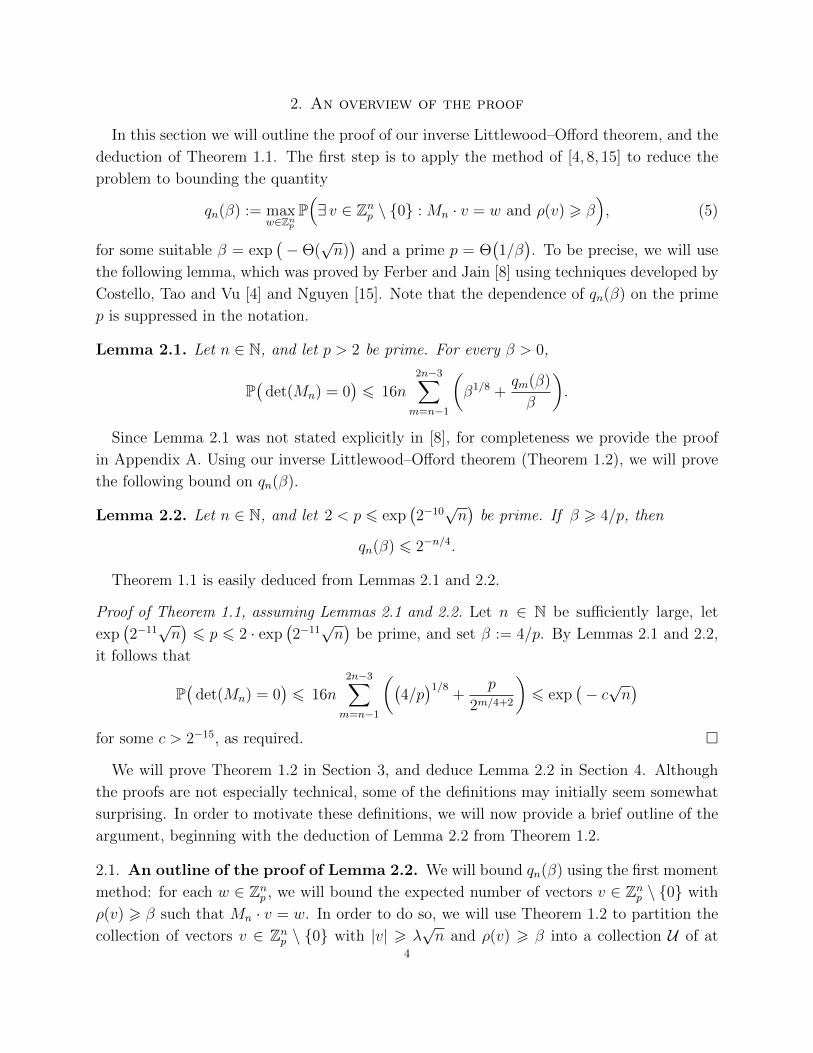
2. An overview of the proof

In this section we will outline the proof of our inverse Littlewood–Offord theorem, and the

deduction of Theorem 1.1. The first step is to apply the method of [4, 8, 15] to reduce the

problem to bounding the quantity

qn(β) := maxw∈Zn

p

P(∃ v ∈ Znp \ 0 : Mn · v = w and ρ(v) > β

), (5)

for some suitable β = exp(− Θ(

√n))

and a prime p = Θ(1/β

). To be precise, we will use

the following lemma, which was proved by Ferber and Jain [8] using techniques developed by

Costello, Tao and Vu [4] and Nguyen [15]. Note that the dependence of qn(β) on the prime

p is suppressed in the notation.

Lemma 2.1. Let n ∈ N, and let p > 2 be prime. For every β > 0,

P(

det(Mn) = 0)6 16n

2n−3∑m=n−1

(β1/8 +

qm(β)

β

).

Since Lemma 2.1 was not stated explicitly in [8], for completeness we provide the proof

in Appendix A. Using our inverse Littlewood–Offord theorem (Theorem 1.2), we will prove

the following bound on qn(β).

Lemma 2.2. Let n ∈ N, and let 2 < p 6 exp(2−10√n)

be prime. If β > 4/p, then

qn(β) 6 2−n/4.

Theorem 1.1 is easily deduced from Lemmas 2.1 and 2.2.

Proof of Theorem 1.1, assuming Lemmas 2.1 and 2.2. Let n ∈ N be sufficiently large, let

exp(2−11√n)6 p 6 2 · exp

(2−11√n)

be prime, and set β := 4/p. By Lemmas 2.1 and 2.2,

it follows that

P(

det(Mn) = 0)6 16n

2n−3∑m=n−1

((4/p)1/8

+p

2m/4+2

)6 exp

(− c√n)

for some c > 2−15, as required.

We will prove Theorem 1.2 in Section 3, and deduce Lemma 2.2 in Section 4. Although

the proofs are not especially technical, some of the definitions may initially seem somewhat

surprising. In order to motivate these definitions, we will now provide a brief outline of the

argument, beginning with the deduction of Lemma 2.2 from Theorem 1.2.

2.1. An outline of the proof of Lemma 2.2. We will bound qn(β) using the first moment

method: for each w ∈ Znp , we will bound the expected number of vectors v ∈ Znp \ 0 with

ρ(v) > β such that Mn · v = w. In order to do so, we will use Theorem 1.2 to partition the

collection of vectors v ∈ Znp \ 0 with |v| > λ√n and ρ(v) > β into a collection U of at

4

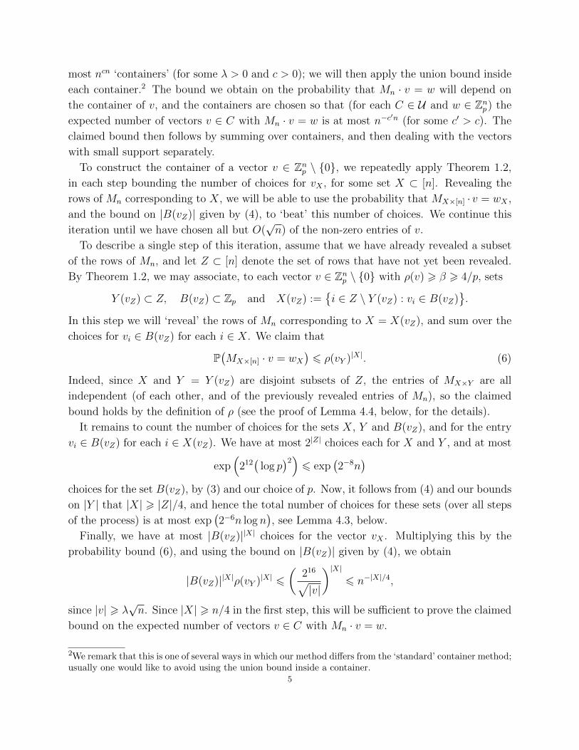
most ncn ‘containers’ (for some λ > 0 and c > 0); we will then apply the union bound inside

each container.2 The bound we obtain on the probability that Mn · v = w will depend on

the container of v, and the containers are chosen so that (for each C ∈ U and w ∈ Znp ) the

expected number of vectors v ∈ C with Mn · v = w is at most n−c′n (for some c′ > c). The

claimed bound then follows by summing over containers, and then dealing with the vectors

with small support separately.

To construct the container of a vector v ∈ Znp \ 0, we repeatedly apply Theorem 1.2,

in each step bounding the number of choices for vX , for some set X ⊂ [n]. Revealing the

rows of Mn corresponding to X, we will be able to use the probability that MX×[n] · v = wX ,

and the bound on |B(vZ)| given by (4), to ‘beat’ this number of choices. We continue this

iteration until we have chosen all but O(√n) of the non-zero entries of v.

To describe a single step of this iteration, assume that we have already revealed a subset

of the rows of Mn, and let Z ⊂ [n] denote the set of rows that have not yet been revealed.

By Theorem 1.2, we may associate, to each vector v ∈ Znp \ 0 with ρ(v) > β > 4/p, sets

Y (vZ) ⊂ Z, B(vZ) ⊂ Zp and X(vZ) :=i ∈ Z \ Y (vZ) : vi ∈ B(vZ)

.

In this step we will ‘reveal’ the rows of Mn corresponding to X = X(vZ), and sum over the

choices for vi ∈ B(vZ) for each i ∈ X. We claim that

P(MX×[n] · v = wX

)6 ρ(vY )|X|. (6)

Indeed, since X and Y = Y (vZ) are disjoint subsets of Z, the entries of MX×Y are all

independent (of each other, and of the previously revealed entries of Mn), so the claimed

bound holds by the definition of ρ (see the proof of Lemma 4.4, below, for the details).

It remains to count the number of choices for the sets X, Y and B(vZ), and for the entry

vi ∈ B(vZ) for each i ∈ X(vZ). We have at most 2|Z| choices each for X and Y , and at most

exp(

212(

log p)2)6 exp

(2−8n

)choices for the set B(vZ), by (3) and our choice of p. Now, it follows from (4) and our bounds

on |Y | that |X| > |Z|/4, and hence the total number of choices for these sets (over all steps

of the process) is at most exp(2−6n log n

), see Lemma 4.3, below.

Finally, we have at most |B(vZ)||X| choices for the vector vX . Multiplying this by the

probability bound (6), and using the bound on |B(vZ)| given by (4), we obtain

|B(vZ)||X|ρ(vY )|X| 6

(216√|v|

)|X|6 n−|X|/4,

since |v| > λ√n. Since |X| > n/4 in the first step, this will be sufficient to prove the claimed

bound on the expected number of vectors v ∈ C with Mn · v = w.

2We remark that this is one of several ways in which our method differs from the ‘standard’ container method;usually one would like to avoid using the union bound inside a container.

5

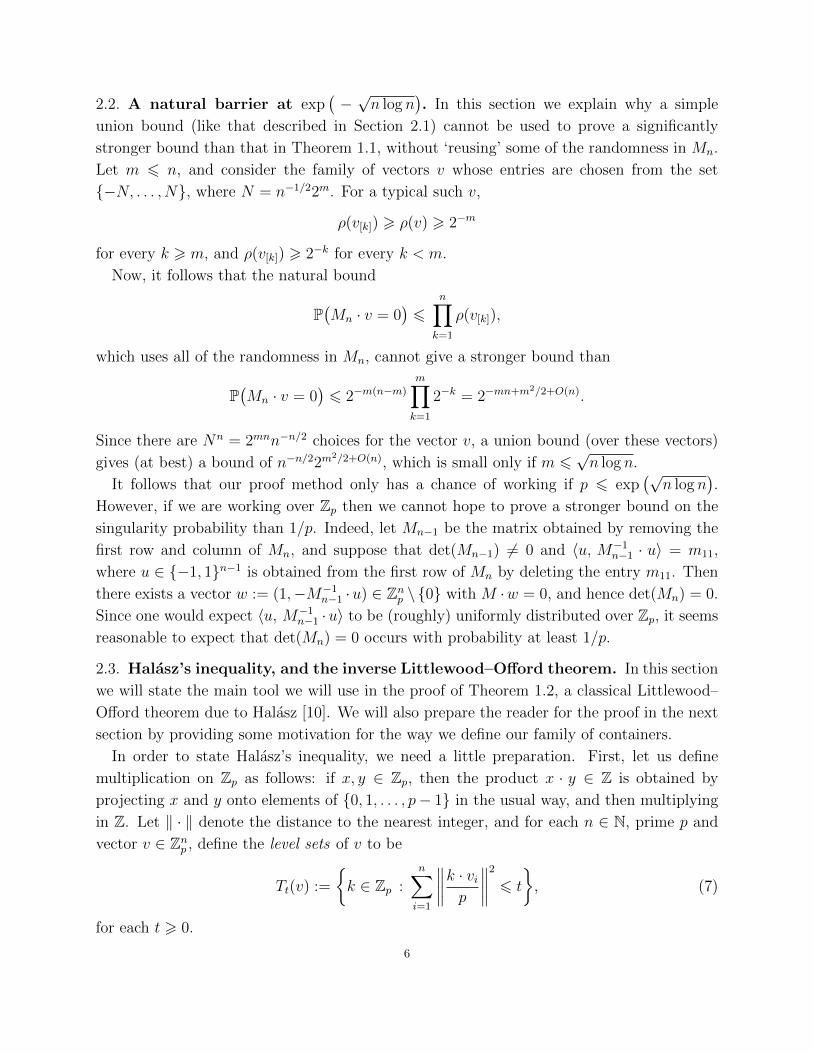
2.2. A natural barrier at exp(−√n log n

). In this section we explain why a simple

union bound (like that described in Section 2.1) cannot be used to prove a significantly

stronger bound than that in Theorem 1.1, without ‘reusing’ some of the randomness in Mn.

Let m 6 n, and consider the family of vectors v whose entries are chosen from the set

−N, . . . , N, where N = n−1/22m. For a typical such v,

ρ(v[k]) > ρ(v) > 2−m

for every k > m, and ρ(v[k]) > 2−k for every k < m.

Now, it follows that the natural bound

P(Mn · v = 0

)6

n∏k=1

ρ(v[k]),

which uses all of the randomness in Mn, cannot give a stronger bound than

P(Mn · v = 0

)6 2−m(n−m)

m∏k=1

2−k = 2−mn+m2/2+O(n).

Since there are Nn = 2mnn−n/2 choices for the vector v, a union bound (over these vectors)

gives (at best) a bound of n−n/22m2/2+O(n), which is small only if m 6

√n log n.

It follows that our proof method only has a chance of working if p 6 exp(√

n log n).

However, if we are working over Zp then we cannot hope to prove a stronger bound on the

singularity probability than 1/p. Indeed, let Mn−1 be the matrix obtained by removing the

first row and column of Mn, and suppose that det(Mn−1) 6= 0 and 〈u, M−1n−1 · u〉 = m11,

where u ∈ −1, 1n−1 is obtained from the first row of Mn by deleting the entry m11. Then

there exists a vector w := (1,−M−1n−1 ·u) ∈ Znp \ 0 with M ·w = 0, and hence det(Mn) = 0.

Since one would expect 〈u, M−1n−1 ·u〉 to be (roughly) uniformly distributed over Zp, it seems

reasonable to expect that det(Mn) = 0 occurs with probability at least 1/p.

2.3. Halasz’s inequality, and the inverse Littlewood–Offord theorem. In this section

we will state the main tool we will use in the proof of Theorem 1.2, a classical Littlewood–

Offord theorem due to Halasz [10]. We will also prepare the reader for the proof in the next

section by providing some motivation for the way we define our family of containers.

In order to state Halasz’s inequality, we need a little preparation. First, let us define

multiplication on Zp as follows: if x, y ∈ Zp, then the product x · y ∈ Z is obtained by

projecting x and y onto elements of 0, 1, . . . , p− 1 in the usual way, and then multiplying

in Z. Let ‖ · ‖ denote the distance to the nearest integer, and for each n ∈ N, prime p and

vector v ∈ Znp , define the level sets of v to be

Tt(v) :=

k ∈ Zp :

n∑i=1

∥∥∥∥k · vip

∥∥∥∥2

6 t

, (7)

for each t > 0.

6

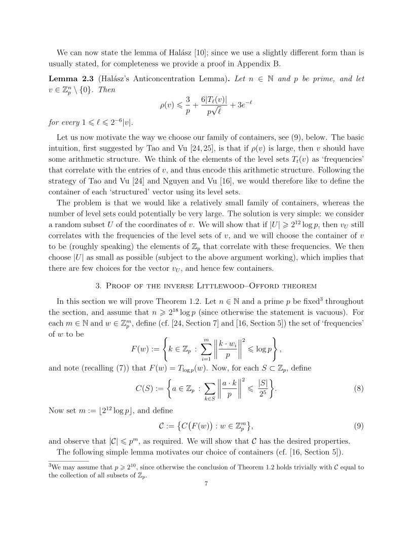
We can now state the lemma of Halasz [10]; since we use a slightly different form than is

usually stated, for completeness we provide a proof in Appendix B.

Lemma 2.3 (Halasz’s Anticoncentration Lemma). Let n ∈ N and p be prime, and let

v ∈ Znp \ 0. Then

ρ(v) 63

p+

6|T`(v)|p√`

+ 3e−`

for every 1 6 ` 6 2−6|v|.

Let us now motivate the way we choose our family of containers, see (9), below. The basic

intuition, first suggested by Tao and Vu [24, 25], is that if ρ(v) is large, then v should have

some arithmetic structure. We think of the elements of the level sets Tt(v) as ‘frequencies’

that correlate with the entries of v, and thus encode this arithmetic structure. Following the

strategy of Tao and Vu [24] and Nguyen and Vu [16], we would therefore like to define the

container of each ‘structured’ vector using its level sets.

The problem is that we would like a relatively small family of containers, whereas the

number of level sets could potentially be very large. The solution is very simple: we consider

a random subset U of the coordinates of v. We will show that if |U | > 212 log p, then vU still

correlates with the frequencies of the level sets of v, and we will choose the container of v

to be (roughly speaking) the elements of Zp that correlate with these frequencies. We then

choose |U | as small as possible (subject to the above argument working), which implies that

there are few choices for the vector vU , and hence few containers.

3. Proof of the inverse Littlewood–Offord theorem

In this section we will prove Theorem 1.2. Let n ∈ N and a prime p be fixed3 throughout

the section, and assume that n > 218 log p (since otherwise the statement is vacuous). For

each m ∈ N and w ∈ Zmp , define (cf. [24, Section 7] and [16, Section 5]) the set of ‘frequencies’

of w to be

F (w) :=

k ∈ Zp :

m∑i=1

∥∥∥∥k · wip

∥∥∥∥2

6 log p

,

and note (recalling (7)) that F (w) = Tlog p(w). Now, for each S ⊂ Zp, define

C(S) :=

a ∈ Zp :

∑k∈S

∥∥∥∥a · kp∥∥∥∥2

6|S|25

. (8)

Now set m := b212 log pc, and define

C :=C(F (w)

): w ∈ Zmp

, (9)

and observe that |C| 6 pm, as required. We will show that C has the desired properties.

The following simple lemma motivates our choice of containers (cf. [16, Section 5]).

3We may assume that p > 210, since otherwise the conclusion of Theorem 1.2 holds trivially with C equal tothe collection of all subsets of Zp.

7

Lemma 3.1. Let v ∈ Znp , and let t 6 2−7n. If S ⊂ Tt(v), then∣∣i ∈ [n] : vi 6∈ C(S)∣∣ 6 n

4.

Proof. Let R =i ∈ [n] : vi /∈ C(S)

, and observe that, by (7) and (8),

|R||S|25

6∑i∈R

∑k∈S

∥∥∥∥k · vip

∥∥∥∥2

6∑k∈S

n∑i=1

∥∥∥∥k · vip

∥∥∥∥2

6n|S|27

,

so |R| 6 n/4, as required.

Later in the proof, we will define B(v) := C(F (vU)

)for some set U ⊂ [n] with |U | 6 m

such that F (vU) ⊂ Tt(v) for t = 2−7n (see Lemma 3.6, below). We next turn to bounding

the size of our containers; the following lemma (cf. [16, Section 5]) provides a first step.

Lemma 3.2. For any set S ⊂ Zp, we have

|C(S)| 6 4p

|S|. (10)

Proof. We will instead bound the size of the larger set

C ′(S) :=

a ∈ Zp :

∑k∈S

cos

(2πak

p

)>|S|2

.

Indeed, observe that C(S) ⊂ C ′(S), since we have 1− 24‖x‖2 6 cos(2πx) for every x ∈ R.

Now, let a be a uniformly-chosen random element of Zp, and observe that, by Markov’s

inequality,

P(a ∈ C ′(S)

)= P

((∑k∈S

cos

(2πak

p

))2

>|S|2

4

)

64

|S|2· 1

p

∑a∈Zp

(∑k∈S

cos

(2πak

p

))2

,

Now, since 2 cos(x) = eix + e−ix, we have

4∑a∈Zp

(∑k∈S

cos

(2πak

p

))2

=∑k1∈±S

∑k2∈±S

∑a∈Zp

exp

(2πia(k1 + k2)

p

)6 4p|S|,

where ±S is the multi-set obtained by taking the union of S and −S, counting elements in

both twice. For the second step, simply note that the roots of unity sum to zero, so the only

terms that contribute are those with k1 + k2 = 0. It follows that

4

|S|2· 1

p

∑a∈Zp

(∑k∈S

cos

(2πak

p

))2

64

|S|,

and hence |C(S)| 6 |C ′(S)| 6 4p/|S|, as claimed. 8

We will use Halasz’s Anticoncentration Lemma (Lemma 2.3) to bound the right-hand side

of (10) in terms of ρ(vY ) (for some set Y that will be chosen in Lemma 3.5, below). The

following lemma is a straightforward application of Lemma 2.3.

Lemma 3.3. Let v ∈ Znp with ρ(v) > 4/p and |v| > 218 log p, and let Y ⊂ [n] be such that

|vY | > |v|/4. Then

ρ(vY ) 6213|T`(vY )|p√|v|

,

where ` := 2−16|v|.

In the proof of Lemma 3.3, and also later in the section, we will need the following simple

observation (see Lemma A.10 or [8, Lemma 2.8]).

Observation 3.4 (Lemma 2.8 of [8]). ρ(vY ) > ρ(v) for every v ∈ Znp and every Y ⊂ [n].

Proof of Lemma 3.3. Applying Lemma 2.3 to vY , with ` = 2−16|v| 6 2−14|vY |, gives

ρ(vY ) 63

p+

6|T`(vY )|p√`

+ 3e−`.

Now, by Observation 3.4 and our assumption on ρ(v), we have ρ(vY ) > ρ(v) > 4/p. Since

` > 4 log p, it follows that

ρ(vY ) 625|T`(vY )|p√`

=213|T`(vY )|p√|v|

,

as claimed.

To complete the proof, it will now suffice to choose sets Y ⊂ [n], with n/4 6 |Y | 6 n/2,

and U ⊂ [n], with |U | 6 m, such that

F (vU) ⊂ Tt(v), |vY | >|v|4

and |T`(vY )| 6 2 · |F (vU)|, (11)

where ` = 2−16|v| and t = 2−7n. Indeed, for any such sets we have, by Lemmas 3.2 and 3.3,∣∣C(F (vU))∣∣ 6 4p

|F (vU)|6

215

ρ(vY )√|v|· |T`(vY )||F (vU)|

6216

ρ(vY )√|v|,

and, by Lemma 3.1, we have ∣∣i ∈ [n] : vi 6∈ C(F (vU)

)∣∣ 6 n

4.

Thus, setting B(v) := C(F (vU)

), we obtain a set in C for which the properties (4) hold.

We will choose the sets Y and U in the next two lemmas. In each case we simply choose

a random set of the correct density. We will say that R is a q-random subset of a set S if

each element of S is included in R independently at random with probability q.

9

Lemma 3.5. Let v ∈ Znp with |v| > 218 log p. There exists Y ⊂ [n], with n/4 6 |Y | 6 n/2,

such that

|vY | >|v|4

and T`(vY ) ⊂ T8`(v),

where ` = 2−16|v|.

Proof. Let Y be a (3/8)-random subset of [n]; we will prove that with positive probability

Y has all of the required properties. Since n > |v| > 218 log p > 218, the properties

n

46 |Y | 6 n

2and |vY | >

|v|4

each hold with probability at least 3/4, by Chernoff’s inequality. To bound the probability

that T`(vY ) \ T8`(v) is non-empty, define a random variable

W (k) :=∑i∈Y

∥∥∥∥k · vip

∥∥∥∥2

for each k ∈ Zp, and observe that, by (7),

k ∈ T`(vY ) ⇔ W (k) 6 ` and k 6∈ T8`(v) ⇒ E[W (k)] > 3`.

Moreover, by Chernoff’s inequality,4

P(k ∈ T`(vY )

)= P

(W (k) 6 `

)6 e−`/2 6

1

p2

for every k 6∈ T8`(v), since ` > 4 log p. It follows that

E[|T`(vY ) \ T8`(v)|

]6

1

p,

and hence T`(vY ) ⊂ T8`(v) with probability at least 3/4, as required.

Finally, we need to show that a suitable set U exists.

Lemma 3.6. Let v ∈ Znp . There exists U ⊂ [n], with |U | 6 m, such that

|T8`(v)| 6 2 · |F (vU)| and F (vU) ⊂ Tt(v),

where ` = 2−16|v| and t = 2−7n.

Proof. Let U be a (m/2n)-random subset of [n]. We will prove that the claimed properties

hold simultaneously with positive probability. Note first that |U | 6 m with probability at

least 3/4, by Chernoff’s inequality, since m = b212 log pc > 212.

Next, we show that |T8`(v) \ F (vU)| 6 |T8`(v)|/2 with probability at least 1/2. Observe

first that, for every k ∈ Zp,

P(k 6∈ F (vU)

)= P

(∑i∈U

∥∥∥∥k · vip

∥∥∥∥2

> log p

)6

1

log p· E

[∑i∈U

∥∥∥∥k · vip

∥∥∥∥2],

4Here we use the following variant of the standard Chernoff inequality: if X1, . . . , XN are iid Bernoulli

random variables, and t1, . . . , tN ∈ [0, 1], then P(∑N

i=1 tiXi 6 s)6 exp

(− E[X]/2 + s

).

10

by Markov’s inequality. Now, if k ∈ T8`(v), then

1

log p· E

[∑i∈U

∥∥∥∥k · vip

∥∥∥∥2]

=m

2n log p

n∑i=1

∥∥∥∥k · vip

∥∥∥∥2

68m`

2n log p6

1

4,

since m 6 212 log p and ` = 2−16|v| 6 2−16n. It follows that

P(|T8`(v) \ F (vU)| > |T8`(v)|

2

)6

2

|T8`(v)|· E[|T8`(v) \ F (vU)|

]6

1

2,

by Markov’s inequality, as claimed.

Finally, to bound the probability that F (vU)\Tt(v) is non-empty, we repeat the argument

used in the proof of Lemma 3.5. To be precise, we define a random variable

W (k) :=∑i∈U

∥∥∥∥k · vip

∥∥∥∥2

for each k ∈ Zp, and observe that, by (7),

k ∈ F (vU) ⇔ W (k) 6 log p and k 6∈ Tt(v) ⇒ E[W (k)] > 2−8m.

Recalling that m = b212 log pc, it follows by Chernoff’s inequality that

P(k ∈ F (vU)

)= P

(W (k) 6 log p

)6

1

p2

for every k 6∈ Tt(v), and hence

P(F (vU) 6⊂ Tt(v)

)6 E

[|F (vU) \ Tt(v)|

]6

1

p.

It follows that, with positive probability, the random set U satisfies

|U | 6 m, |T8`(v)| 6 2 · |F (vU)| and F (vU) ⊂ Tt(v),

as required.

As observed above, it is now straightforward to complete the proof of Theorem 1.2.

Proof of Theorem 1.2. Let C be as defined in (9), and note that

|C| 6 pm 6 exp(212(log p)2

).

For each v ∈ Znp with ρ(v) > 4/p and |v| > 218 log p, let Y and U be the sets given by

Lemmas 3.5 and 3.6 respectively, and define B(v) := C(F (vU)

). Now, we have n/4 6 |Y | 6

n/2, by Lemma 3.5, and ∣∣i ∈ [n] : vi 6∈ B(v)∣∣ 6 n

4,

by Lemma 3.1, since F (vU) ⊂ Tt(v), where t = 2−7n, by Lemma 3.6. Finally, we have

|B(v)| 6 4p

|F (vU)|6

215

ρ(vY )√|v|· |T`(vY )||F (vU)|

6216

ρ(vY )√|v|,

by Lemmas 3.2–3.6, since |T`(vY )| 6 |T8`(v)| 6 2 · |F (vU)|. This completes the proof of the

inverse Littlewood–Offord theorem. 11

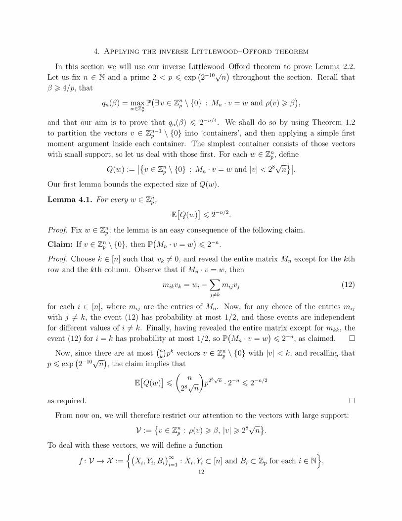
4. Applying the inverse Littlewood–Offord theorem

In this section we will use our inverse Littlewood–Offord theorem to prove Lemma 2.2.

Let us fix n ∈ N and a prime 2 < p 6 exp(2−10√n)

throughout the section. Recall that

β > 4/p, that

qn(β) = maxw∈Zn

p

P(∃ v ∈ Znp \ 0 : Mn · v = w and ρ(v) > β

),

and that our aim is to prove that qn(β) 6 2−n/4. We shall do so by using Theorem 1.2

to partition the vectors v ∈ Zn−1p \ 0 into ‘containers’, and then applying a simple first

moment argument inside each container. The simplest container consists of those vectors

with small support, so let us deal with those first. For each w ∈ Znp , define

Q(w) :=∣∣v ∈ Znp \ 0 : Mn · v = w and |v| < 28

√n∣∣.

Our first lemma bounds the expected size of Q(w).

Lemma 4.1. For every w ∈ Znp ,

E[Q(w)

]6 2−n/2.

Proof. Fix w ∈ Znp ; the lemma is an easy consequence of the following claim.

Claim: If v ∈ Znp \ 0, then P(Mn · v = w

)6 2−n.

Proof. Choose k ∈ [n] such that vk 6= 0, and reveal the entire matrix Mn except for the kth

row and the kth column. Observe that if Mn · v = w, then

mikvk = wi −∑j 6=k

mijvj (12)

for each i ∈ [n], where mij are the entries of Mn. Now, for any choice of the entries mij

with j 6= k, the event (12) has probability at most 1/2, and these events are independent

for different values of i 6= k. Finally, having revealed the entire matrix except for mkk, the

event (12) for i = k has probability at most 1/2, so P(Mn · v = w

)6 2−n, as claimed.

Now, since there are at most(nk

)pk vectors v ∈ Znp \ 0 with |v| < k, and recalling that

p 6 exp(2−10√n), the claim implies that

E[Q(w)

]6

(n

28√n

)p28√n · 2−n 6 2−n/2

as required.

From now on, we will therefore restrict our attention to the vectors with large support:

V :=v ∈ Znp : ρ(v) > β, |v| > 28

√n.

To deal with these vectors, we will define a function

f : V → X :=(Xi, Yi, Bi

)∞i=1

: Xi, Yi ⊂ [n] and Bi ⊂ Zp for each i ∈ N,

12

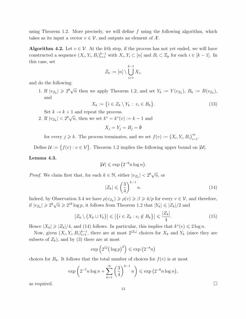
using Theorem 1.2. More precisely, we will define f using the following algorithm, which

takes as its input a vector v ∈ V , and outputs an element of X .

Algorithm 4.2. Let v ∈ V . At the kth step, if the process has not yet ended, we will have

constructed a sequence (Xi, Yi, Bi)k−1i=1 with Xi, Yi ⊂ [n] and Bi ⊂ Zp for each i ∈ [k − 1]. In

this case, set

Zk := [n] \k−1⋃i=1

Xi,

and do the following:

1. If |vZk| > 28

√n then we apply Theorem 1.2, and set Yk := Y (vZk

), Bk := B(vZk),

and

Xk :=i ∈ Zk \ Yk : vi ∈ Bk

. (13)

Set k → k + 1 and repeat the process.

2. If |vZk| < 28

√n, then we set k∗ = k∗(v) := k − 1 and

Xj = Yj = Bj = ∅

for every j > k. The process terminates, and we set f(v) :=(Xi, Yi, Bi

)∞i=1

.

Define U :=f(v) : v ∈ V

. Theorem 1.2 implies the following upper bound on |U|.

Lemma 4.3.

|U| 6 exp(2−6n log n

).

Proof. We claim first that, for each k ∈ N, either |vZk| < 28

√n, or

|Zk| 6(

3

4

)k−1

n. (14)

Indeed, by Observation 3.4 we have ρ(vZk) > ρ(v) > β > 4/p for every v ∈ V , and therefore,

if |vZk| > 28

√n > 218 log p, it follows from Theorem 1.2 that |Yk| 6 |Zk|/2 and∣∣Zk \ (Xk ∪ Yk

)∣∣ 6 ∣∣i ∈ Zk : vi /∈ Bk

∣∣ 6 |Zk|4. (15)

Hence |Xk| > |Zk|/4, and (14) follows. In particular, this implies that k∗(v) 6 2 log n.

Now, given (Xi, Yi, Bi)k−1i=1 , there are at most 2|Zk| choices for Xk and Yk (since they are

subsets of Zk), and by (3) there are at most

exp(

212(

log p)2)6 exp

(2−8n

)choices for Bk. It follows that the total number of choices for f(v) is at most

exp

(2−7n log n+

∞∑k=1

(3

4

)k−1

n

)6 exp

(2−6n log n

),

as required. 13

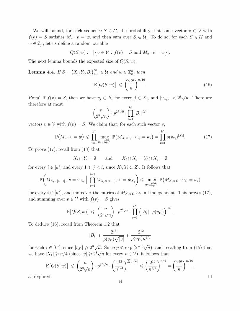
We will bound, for each sequence S ∈ U , the probability that some vector v ∈ V with

f(v) = S satisfies Mn · v = w, and then sum over S ∈ U . To do so, for each S ∈ U and

w ∈ Znp , let us define a random variable

Q(S,w) :=∣∣v ∈ V : f(v) = S and Mn · v = w

∣∣.The next lemma bounds the expected size of Q(S,w).

Lemma 4.4. If S =(Xi, Yi, Bi

)∞i=1∈ U and w ∈ Znp , then

E[Q(S,w)

]6

(256

n

)n/16

. (16)

Proof. If f(v) = S, then we have vj ∈ Bi for every j ∈ Xi, and |vZk∗ | < 28√n. There are

therefore at most (n

28√n

)· p28

√n ·

k∗∏i=1

|Bi||Xi|

vectors v ∈ V with f(v) = S. We claim that, for each such vector v,

P(Mn · v = w

)6

k∗∏i=1

maxwi∈Z

|Xi|p

P(MXi×Yi · vYi = wi

)=

k∗∏i=1

ρ(vYi)|Xi|. (17)

To prove (17), recall from (13) that

Xi ∩ Yi = ∅ and Xi ∩Xj = Yi ∩Xj = ∅

for every i ∈ [k∗] and every 1 6 j < i, since Xi, Yi ⊂ Zi. It follows that

P(MXi×[n−1] · v = wXi

∣∣∣ i−1⋂j=1

MXj×[n−1] · v = wXj

)6 max

wi∈Z|Xi|p

P(MXi×Yi · vYi = wi

)for every i ∈ [k∗], and moreover the entries of MXi×Yi are all independent. This proves (17),

and summing over v ∈ V with f(v) = S gives

E[Q(S,w)

]6

(n

28√n

)· p28

√n ·

k∗∏i=1

(|Bi| · ρ(vYi)

)|Xi|.

To deduce (16), recall from Theorem 1.2 that

|Bi| 6216

ρ(vY )√|v|6

212

ρ(vYi)n1/4

for each i ∈ [k∗], since |vZi| > 28

√n. Since p 6 exp

(2−10√n), and recalling from (15) that

we have |X1| > n/4 (since |v| > 28√n for every v ∈ V), it follows that

E[Q(S,w)

]6

(n

28√n

)· p28

√n ·(

212

n1/4

)∑i |Xi|

6

(214

n1/4

)n/4=

(256

n

)n/16

,

as required. 14

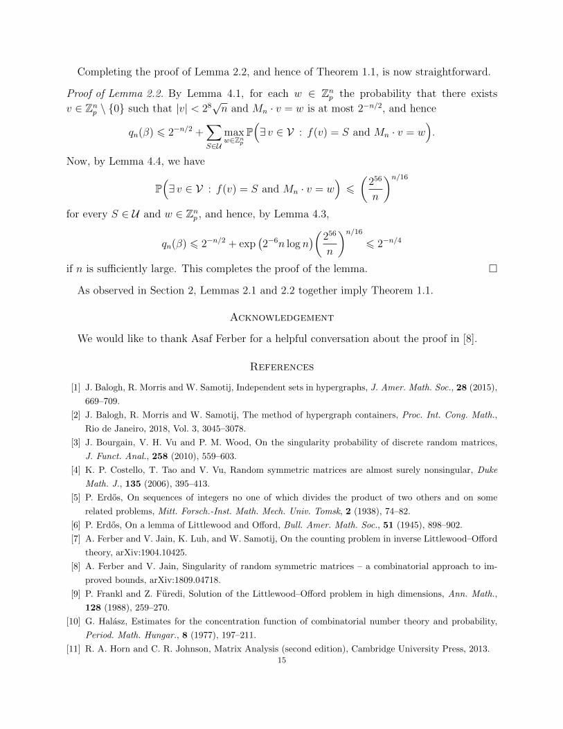
Completing the proof of Lemma 2.2, and hence of Theorem 1.1, is now straightforward.

Proof of Lemma 2.2. By Lemma 4.1, for each w ∈ Znp the probability that there exists

v ∈ Znp \ 0 such that |v| < 28√n and Mn · v = w is at most 2−n/2, and hence

qn(β) 6 2−n/2 +∑S∈U

maxw∈Zn

p

P(∃ v ∈ V : f(v) = S and Mn · v = w

).

Now, by Lemma 4.4, we have

P(∃ v ∈ V : f(v) = S and Mn · v = w

)6

(256

n

)n/16

for every S ∈ U and w ∈ Znp , and hence, by Lemma 4.3,

qn(β) 6 2−n/2 + exp(2−6n log n

)(256

n

)n/16

6 2−n/4

if n is sufficiently large. This completes the proof of the lemma.

As observed in Section 2, Lemmas 2.1 and 2.2 together imply Theorem 1.1.

Acknowledgement

We would like to thank Asaf Ferber for a helpful conversation about the proof in [8].

References

[1] J. Balogh, R. Morris and W. Samotij, Independent sets in hypergraphs, J. Amer. Math. Soc., 28 (2015),

669–709.

[2] J. Balogh, R. Morris and W. Samotij, The method of hypergraph containers, Proc. Int. Cong. Math.,

Rio de Janeiro, 2018, Vol. 3, 3045–3078.

[3] J. Bourgain, V. H. Vu and P. M. Wood, On the singularity probability of discrete random matrices,

J. Funct. Anal., 258 (2010), 559–603.

[4] K. P. Costello, T. Tao and V. Vu, Random symmetric matrices are almost surely nonsingular, Duke

Math. J., 135 (2006), 395–413.

[5] P. Erdos, On sequences of integers no one of which divides the product of two others and on some

related problems, Mitt. Forsch.-Inst. Math. Mech. Univ. Tomsk, 2 (1938), 74–82.

[6] P. Erdos, On a lemma of Littlewood and Offord, Bull. Amer. Math. Soc., 51 (1945), 898–902.

[7] A. Ferber and V. Jain, K. Luh, and W. Samotij, On the counting problem in inverse Littlewood–Offord

theory, arXiv:1904.10425.

[8] A. Ferber and V. Jain, Singularity of random symmetric matrices – a combinatorial approach to im-

proved bounds, arXiv:1809.04718.

[9] P. Frankl and Z. Furedi, Solution of the Littlewood–Offord problem in high dimensions, Ann. Math.,

128 (1988), 259–270.

[10] G. Halasz, Estimates for the concentration function of combinatorial number theory and probability,

Period. Math. Hungar., 8 (1977), 197–211.

[11] R. A. Horn and C. R. Johnson, Matrix Analysis (second edition), Cambridge University Press, 2013.15

[12] J. Kahn, J. Komlos and E. Szemeredi, On the probability that a random ±1 matrix is singular,

J. Amer. Math. Soc., 8 (1995), 223–240.

[13] J. Komlos, On the determinant of (0, 1) matrices, Studia Sci. Math. Hungar., 2 (1967), 7–22.

[14] J. E. Littlewood and A. C. Offord, On the number of real roots of a random algebraic equation III,

Rec. Math. (Mat. Sbornik) N.S., 12 (1943), 277–286.

[15] H. H. Nguyen, Inverse Littlewood–Offord problems and the singularity of random symmetric matrices,

Duke Math. J., 161 (2012), 545–586.

[16] H. H. Nguyen and V. H. Vu, Optimal inverse Littlewood–Offord theorems, Adv. Math., 226 (2011),

5298–5319.

[17] H. H. Nguyen and V. H. Vu, Small ball probability, inverse theorems, and applications, In: Erdos

Centennial, pages 409–463. Springer, 2013.

[18] A. M. Odlyzko, On subspaces spanned by random selections of ±1 vectors, J. Combin. Theory Ser. A,

47 (1988), 124–133.

[19] M. Rudelson, Invertibility of random matrices: norm of the inverse, Ann. Math., 168 (2008), 575–600.

[20] M. Rudelson and R. Vershynin, The Littlewood–Offord problem and invertibility of random matrices,

Adv. Math., 218 (2008), 600–633.

[21] M. Rudelson and R. Vershynin, Smallest singular value of a random rectangular matrix, Comm. Pure

Appl. Math., 62 (2009), 1707–1739.

[22] M. Rudelson and R. Vershynin, Non-asymptotic theory of random matrices: extreme singular values,

Proc. Int. Cong. Math., Hyderabad, 2010, Vol. 3, 1576–1602.

[23] D. Saxton and A. Thomason, Hypergraph containers, Inv. Math., 201 (2015), 1–68.

[24] T. Tao and V. Vu, On the singularity probability of random Bernoulli matrices, J. Amer. Math. Soc.,

20 (2007), 603–628.

[25] T. Tao and V. Vu, Inverse Littlewood–Offord theorems and the condition number of random discrete

matrices, Ann. Math., 169 (2009), 595–632.

[26] T. Tao and V. Vu, From the Littlewood–Offord problem to the circular law: universality of the spectral

distribution of random matrices, Bull. Amer. Math. Soc., 46 (2009), 377–396.

[27] K. Tikhomirov, Singularity of random Bernoulli matrices, arXiv:1812.09016.

[28] R. Vershynin, Invertibility of symmetric random matrices, Random Structures Algorithms, 44 (2014),

135–182.

[29] V. Vu, Combinatorial problems in random matrix theory, Proc. Int. Cong. Math., Seoul, 2014, Vol. 4,

489–508.

Appendix A. Proof of Lemma 2.1

In this appendix we will provide a proof of Lemma 2.1, which allowed us to reduce the

problem of bounding the probability that det(Mn) = 0 to the problem of bounding qn(β).

The proof given below is essentially contained in the paper of Ferber and Jain [8], and several

of the key lemmas appeared in the papers of Costello, Tao and Vu [4] and Nguyen [15].

However, for the benefit of the reader who is unfamiliar with the area, and since Lemma 2.1

was not stated explicitly in [8], we will provide the details in full. We begin by giving an

overview of the proof.16

A.1. Overview of the proof of Lemma 2.1. It will be convenient in this section to work

over Fp; in particular, we will consider the entries of Mn as elements of Fp, noting that doing

so can only increase the probability that Mn is singular. Observe also that

qn(β) = maxw∈Fn

p

P(∃ v ∈ Fnp \ 0 : Mn · v = w and ρ(v) > β

), (18)

where now Mn is a matrix over Fp.Let us write rk(M) for the rank of a matrixM over Fp, andMn−1 for the random symmetric

matrix obtained by removing the first row and column from Mn. The following lemma, which

was proved by Nguyen (see [15, Section 2]), allows us to restrict our attention to matrices

Mn such that rk(Mn) = n− 1 and rk(Mn−1) ∈ n− 2, n− 1.

Lemma A.1. For every n ∈ N and prime p > 2,

P(

det(Mn) = 0)6 4n

2n−2∑m=n

P(

rk(Mm) = m− 1∩

rk(Mm−1) ∈ m− 2,m− 1).

The proof of Lemma A.1 is given in Section A.2. The next two lemmas deal with the cases

rk(Mn−1) = n− 2 and rk(Mn−1) = n− 1 respectively; the first is more straightforward.

Lemma A.2. For every n ∈ N, prime p > 2, and β > 0,

P(

rk(Mn) = n− 1∩

rk(Mn−1) = n− 2)6 β + qn−1(β).

The proof of Lemma A.2, which follows that given in [8, Section 2.2], is described in

Section A.3. Finally, the following lemma deals with the case rk(Mn−1) = n− 1.

Lemma A.3. For every n ∈ N, prime p > 2, β > 0, and integer 1 6 k 6 n− 2, we have

P(

rk(Mn) = rk(Mn−1) = n− 1)6 2 ·

(2kβ + 2−k

)1/4+ 3k+1qn−1(β).

The proof of Lemma A.3, which is similar to that given in [8, Section 2.3], is provided in

Section A.4. Combining Lemmas A.1, A.2 and A.3, we obtain Lemma 2.1.

Proof of Lemma 2.1. Observe first that qn(β) > 2−n for every β < 1/2 (to see this, set

v = (1, 0, . . . , 0)), so the claimed bound holds trivially if β > n−1 or β < 2−n. We may

therefore assume that k := blog4(1/β)c ∈ [n − 2], and therefore, by Lemmas A.1, A.2

and A.3, we obtain

P(

det(An) = 0)6 4n

2n−2∑m=n

(β + qm−1(β) + 2 ·

(3β1/2

)1/4+ β−1qm−1(β)

)6 16n

2n−3∑m=n−1

(β1/8 +

qm(β)

β

).

as required. 17

A.2. The proof of Lemma A.1. As noted above, Lemma A.1 is a straightforward conse-

quence of [15, Lemmas 2.1 and 2.3]. The first of these two lemmas is as follows.

Lemma A.4 (Lemma 2.1 of [15]). For any 0 6 k 6 n− 1,

P(rk(Mn) = k

)6 2 · P

(rk(M2n−k−1) = 2n− k − 2

). (19)

To prove Lemma A.4 we will need the following observation of Odlyzko [18]; since it is

usually stated in Rn, we provide the short proof.

Observation A.5. Let V be a subspace of Fnp of dimension at most k. Then∣∣V ∩ −1, 1n∣∣ 6 2k.

Proof. Form an n × k matrix over Fp whose columns are a basis v(1), . . . , v(k) of V , and

choose k linearly independent rows. We obtain an invertible matrix A, and so for each

b ∈ −1, 1k, there is a unique solution in Fkp to the set of equations Ax = b. The 2k vectors∑ki=1 xiv

(i) (one for each b ∈ −1, 1k) are the only possible elements of V ∩ −1, 1n.

We can now prove Lemma A.4.

Proof of Lemma A.4. We claim that, for any 0 6 k 6 n− 1,

P(rk(Mn+1) = k + 2

∣∣ rk(Mn) = k)> 1− 2k−n. (20)

where we remind the reader that Mn is obtained from Mn+1 by removing the first row and

column. Let W be the subspace spanned by the rows of Mn, and note that, by Observa-

tion A.5, if rk(Mn) = k then W intersects −1, 1n in at most 2k vectors.

Let v ∈ Fnp be the vector formed by removing the first element from the first row of Mn+1.

By the remarks above, it follows that P(v /∈ W ) > 1 − 2k−n. We claim that if v 6∈ W then

rk(Mn+1) = k + 2. To see this, note first that if v 6∈ W then the rank of the final n columns

of Mn+1 is k + 1. Now, since Mn+1 is symmetric, the first column of Mn+1 is the same as

the first row, and if v 6∈ W then v is not in the span of the columns of Mn. It follows that

rk(Mn+1) = k + 2, as claimed, and (20) follows.

It follows immediately from (20) that

P(rk(Mn+t) = k + 2t

∣∣ rk(Mn+t−1) = k + 2t− 2))> 1− 2k+t−n−1

for every k > 0 and 1 6 t 6 n − k. Now, building Mn+t from Mn by adding one row and

column at a time, it follows that

P(rk(M2n−k−1) = 2n− k − 2

∣∣ rk(Mn) = k)>

n−k∏i=2

(1− 2−i) >1

2,

which implies (19).

We can now deduce Lemma A.1 using [15, Lemma 2.3], which is the following observation.

Let us write M(i)n for the (symmetric) matrix obtained from Mn by removing the ith row

and the ith column.18

Lemma A.6 (Lemma 2.3 of [15]). If rk(Mn) = n− 1, then maxi∈[n] rk(M(i)n ) > n− 2.

Proof. Choose n− 1 rows of Mn whose span has dimension n− 1, and remove the remaining

row, giving an (n − 1) × n matrix of rank n − 1. Hence, removing any column from this

matrix, we obtain a matrix of rank at least n− 2.

Proof of Lemma A.1. By Lemma A.4, we have

P(

det(Mn) = 0)

=n−1∑k=1

P(rk(Mn) = k

)6 2

n−1∑k=1

P(rk(M2n−k−1) = 2n− k − 2

). (21)

We therefore need to bound P(rk(Mm) = m− 1

)for each n 6 m 6 2n− 2. By Lemma A.6,

and by symmetry, we have

P(rk(Mm) = m− 1) 6

m∑i=1

P(

rk(Mm) = m− 1∩

rk(M (i)m ) > m− 2

)6 m · P

(rk(Mm) = m− 1

∩

rk(Mm−1) ∈ m− 2,m− 1).

Combining this with (21) gives the statement of the lemma.

A.3. The case rk(Mn−1) = n − 2. In this subsection we will prove Lemma A.2, following

the presentation in [8, Section 2.2]. Let us write adj(M) for the adjugate of a matrix M over

Fp. We will need the following lemma of Nguyen [15], see [8, Lemma 2.5].

Lemma A.7. If rk(Mn−1) = n − 2, then there exists a non-trivial column a ∈ Fn−1p of

adj(Mn−1) such that

(a) Mn−1 · a = 0, and

(b) if det(Mn) = 0, then∑n

i=2 aixi = 0,

where a = (a2, . . . , an), and (x1, . . . , xn) is the first row of Mn.

Proof. Recall (see, e.g., [11, page 22]) that if rk(Mn−1) = n− 2, then

Mn−1 · adj(Mn−1) = 0 and rk(adj(Mn−1)

)= 1.

It follows that there exists a non-trivial column vector a of adj(Mn−1), and Mn−1 · a = 0.

To show that property (b) holds, recall that, since Mn is symmetric,

det(Mn) = x1 det(Mn−1)−∑

26i,j6n

cijxixj,

where cij are the entries of adj(Mn−1). Since adj(Mn−1) is a symmetric matrix of rank 1, its

entries can be written in the form cij = λaiaj for some λ ∈ Fp \ 0. Hence

0 =∑

26i,j6n

aiajxixj =

( ∑26i6n

aixi

)2

, (22)

since det(Mn−1) = det(Mn) = 0, as required. 19

We now use Lemma A.7 to deduce Lemma A.2, cf. [8, Section 2.2].

Proof of Lemma A.2. By Lemma A.7, it follows that in order to bound the probability that

rk(Mn) = n− 1 and rk(Mn−1) = n− 2, it suffices to bound the probability that there exists

a vector a ∈ Fn−1p \ 0 (unique up to a constant factor) with Mn−1 · a = 0 and a · x = 0,

where x ∈ −1, 1n−1 is a random vector chosen uniformly and independent of Mn−1.

We will partition this event into ‘structured’ and ‘unstructured’ cases, using the event

Uβ :=ρ(v) 6 β for every vector v ∈ Fn−1

p \ 0 with Mn−1 · v = 0.

Observe first that, for any Mn−1 ∈ Uβ, and any a ∈ Fn−1p \ 0 with Mn−1 · a = 0, we have

P(a · x = 0

∣∣Mn−1

)6 β,

and hence

P(

rk(Mn) = n− 1∩

rk(Mn−1) = n− 2∩ Uβ

)6 β.

On the other hand, by the definition (18) of qn(β), we have

P(U cβ)

= P(∃ v ∈ Fn−1

p \ 0 : Mn−1 · v = 0 and ρ(v) > β)6 qn−1(β).

It follows that

P(

rk(Mn) = n− 1∩

rk(Mn−1) = n− 2)6 β + qn−1(β),

as required.

A.4. The case rk(Mn−1) = n − 1. It only remains to prove Lemma A.3. The strategy is

similar to that used in the previous subsection (in particular, we will split our event into a

‘structured’ case and an ‘unstructured’ case), but now it is trickier to relate our event to

qn(β), as we do not have the simple factorisation of the determinant used in Lemma A.7.

Instead, we will apply the following ‘decoupling’ lemma of Costello, Tao and Vu [4].

Lemma A.8 (Lemma 4.7 of [4]). Let X and Y be independent random variables, and let

E(X, Y ) be an event that depends on X and Y . Then

P(E(X, Y )

)6(P(E(X, Y ) ∩ E(X ′, Y ) ∩ E(X, Y ′) ∩ E(X ′, Y ′)

))1/4

,

where X ′ and Y ′ are independent copies of X and Y .

It was remarked in [4] that Lemma A.8 is equivalent to the classical fact (which was

essentially proved by Erdos [5] in 1938) that a bipartite graph with parts of size m and

n and cmn edges contains at least c4m2n2 (possibly degenerate) copies of C4. Indeed, to

deduce Lemma A.8 from this theorem, simply define a bipartite graph, each of whose vertices

represents an element of the range of X or Y , and whose edges encode the event E .

In order to state the key technical lemma that we will use to prove Lemma A.3, we need

a little notation. Given a vector v ∈ Fmp and a set J ⊂ [m], let vJ ∈ F|J |p denote the

restriction of v to the coordinates of J , and let v∗J be the vector in Fmp whose ith coordinate20

is vi · 1[i ∈ J ]. Moreover, let u, u′ ∈ −1, 1n−1 be chosen uniformly and independently at

random, and define w ∈ −2, 0, 2n−1 by setting wi := ui − u′i for each i ∈ [n− 1].

The following lemma was essentially proved in [4, Section 4.6] (see also [8, Section 2.3]).

Lemma A.9. For any non-trivial partition I ∪ J = [n− 1], we have

P(rk(Mn) = rk(Mn−1) = n− 1

)6 2 · E

[maxa∈Fp

P(zI ·wI = a

∣∣Mn−1

)1/41[rk(Mn−1) = n− 1

]],

where z := M−1n−1 · w∗J , and the expectation is over the choice of Mn−1.

Proof. Let X := (ui)i∈I and Y := (ui)i∈J be random variables, and note that u is determined

by X and Y . Now define, for each choice of Mn−1, an event

E(X, Y ) :=∃ v ∈ Fn−1

p : Mn−1 · v = u and u · v ∈ −1, 1

depending on X and Y . We claim that if rk(Mn−1) = n − 1, and the first row of Mn is

(x1, u1, . . . , un−1) for some x1 ∈ −1, 1, thenrk(Mn) = n− 1

⇒u ∈ E(X, Y )

.

Indeed, since det(Mn) = 0 6= det(Mn−1) there exists a vector v ∈ Fnp such that Mn · v = 0

and v1 = −1. Letting v′ = (v2, . . . , vn), we see that Mn−1 · v′ = u and u · v′ ∈ −1, 1.Now, for each choice of Mn−1, define5

E1 := E(X, Y ) ∩ E(X ′, Y ) ∩ E(X, Y ′) ∩ E(X ′, Y ′).

By Lemma A.8, we have

P(E(X, Y )

∣∣Mn−1

)6 P

(E1

∣∣Mn−1

)1/4,

and hence

P(

rk(Mn) = rk(Mn−1) = n− 1)6 E

[P(E(X, Y )

∣∣Mn−1

)1[rk(Mn−1) = n− 1

]]6 E

[P(E1

∣∣Mn−1

)1/41[rk(Mn−1) = n− 1

]],

where the expectation is over the choice of Mn−1.

To complete the proof of the lemma, it will therefore suffice to show that

P(E1

∣∣Mn−1

)6 16 ·max

a∈Fp

P(zI · wI = a

∣∣Mn−1

)(23)

for all Mn−1 with rk(Mn−1) = n− 1. To prove (23), let us fix Mn−1 (arbitrarily among those

with rk(Mn−1) = n−1) and set A := M−1n−1 and D := −1, 1. We claim that if u ∈ E(X, Y ),

then uTAu ∈ D. To see this, simply observe that

uTAu = uTA ·Mn−1v = uTv ∈ −1, 1 = D.

Recalling that u = u(X, Y ), define f(X, Y ) := uTAu, and observe that if E1 holds, then

f(X, Y )− f(X ′, Y )− f(X, Y ′) + f(X ′, Y ′) ∈ 2D − 2D, (24)

5Here we set X ′ := (u′i)i∈I and Y ′ := (u′i)i∈J , so X ′ and Y ′ are independent copies of X and Y .21

by the observation above. We claim that the left-hand side of (24) is equal to 2zI · wI . To

see this, note that

f(X, Y ) = uTAu =∑

16i,j6n−1

Aijuiuj,

and (abusing notation) let us write f(X, Y )ij := Aijuiuj. Now, observe that if i, j ∈ I, then

f(X, Y )ij = f(X, Y ′)ij and f(X ′, Y )ij = f(X ′, Y ′)ij, and therefore∑i,j∈I

f(X, Y )ij − f(X ′, Y )ij − f(X, Y ′)ij + f(X ′, Y )ij = 0.

Similarly, if i, j ∈ J then f(X, Y )ij = f(X ′, Y )ij and f(X, Y ′)ij = f(X ′, Y ′)ij, and hence

f(X, Y )− f(X ′, Y )− f(X, Y ′) + f(X ′, Y ′) = 2∑i∈I

∑j∈J

Aij(ui − u′i)(uj − u′j).

Recalling that w = u− u′ and zi :=∑

j∈J Aijwj, it follows that

zI · wI =∑i∈I

(ui − u′i)∑j∈J

Aij(uj − u′j),

so the left-hand side of (24) is equal to 2zI · wI , as claimed. Since |D| = 2, it follows that

P(E1

∣∣Mn−1

)6 16 ·max

a∈Fp

P(zI · wI = a

∣∣Mn−1

),

as claimed. As noted above, this completes the proof of the lemma.

In the proof of Lemma A.3 we will need the following variant of ρ(v). For any n ∈ N and

v ∈ Fnp , define

ρ1/2(v) := maxa∈Fp

P(u1v1 + · · ·+ unvn = a

),

where u1, . . . , un are iid random variables taking the value 0 with probability 1/2, and the

values ±1 each with probability 1/4. We will need the following simple inequalities.

Lemma A.10 (Lemma 2.8 and 2.9 of [8]). For any v ∈ Fnp , and any partition I ∪ J = [n],

ρ1/2(v) 6 ρ(v) and ρ(v) 6 ρ(vI) 6 2|J |ρ(v).

Proof. Observe first that

ρ(v) 6∑

w∈−1,1|J|P(uJ = w

)·maxa∈Fp

P(uI · vI = a− w · vJ

∣∣uJ = w)6 ρ(vI).

Since ρ1/2(v) = ρ(v ⊕ v), it follows that ρ1/2(v) 6 ρ(v). Finally, if a ∈ Fp maximises

P(uI · vI = a

), then

ρ(vI) = 2|J | · P(uI · vI = a

)∏j∈J

P(uj = 1

)6 2|J | · P

(u · v = a+

∑j∈J

vj

)6 2|J | · ρ(v),

as claimed.

22

We are now ready to prove our final lemma, cf. [8, Section 2.3].

Proof of Lemma A.3. Recall that 1 6 k 6 n − 2, and let J ⊂ [n − 1] with |J | = k. By

Lemma A.9, it will suffice to show that

E[

maxa∈Fp

P(zI · wI = a

∣∣Mn−1

)1/41[rk(Mn−1) = n− 1

]]6(2|J |β + 2−|J |

)1/4+ 3|J |qn−1(β),

where I = [n] \ J and z = M−1n−1 · w∗J is defined whenever rk(Mn−1) = n − 1. Recall that

w ∈ −2, 0, 2n−1, and observe that therefore Mn−1 · z = w∗J ∈ W (J), where

W (J) :=v ∈ −2, 0, 2n−1 : vj = 0 for all j 6∈ J

.

We will use the following event to partition into cases:

U (J)β :=

ρ(v) 6 β for every vector v ∈ Fn−1

p \ 0 such that Mn−1 · v ∈ W (J).

We will bound the expectation above using the following three claims.

Claim 1: P(Mn−1 6∈ U (J)

β

)6 3|J |qn−1(β).

Proof of Claim 1. If U (J)β does not hold for Mn−1, then there exists a vector v ∈ Fn−1

p \ 0such that Mn−1 · v ∈ W (J) and ρ(v) > β. For each individual vector w ∈ W (J), the

probability that this holds with Mn−1 · v = w is at most qn−1(β), by (18). Hence, summing

over w ∈ W (J), and noting that |W (J)| = 3|J |, the claim follows.

Claim 2: If rk(Mn−1) = n− 1, then P(z = 0

∣∣Mn−1

)6 2−|J |.

Proof of Claim 2. If z = 0 then w∗J = Mn−1 · z = 0. Since wi = 0 occurs with probability

1/2 for each i ∈ J , and these events are independent, the claim follows immediately.

Claim 3: If Mn−1 ∈ U (J)β and rk(Mn−1) = n− 1, then

maxa∈Fp

P(zI · wI = a

∩z 6= 0

∣∣Mn−1

)6 2|J |β.

Proof of Claim 3. Recall that wJ and Mn−1 together determine z, and that the entries of wIare independent of wJ , and observe that ρ1/2(zI) = maxa∈Fp P

(zI · wI = a

). Therefore

P(zI · wI = a

∩z 6= 0

∣∣Mn−1

)6 E

[ρ1/2(zI)1

[z 6= 0

] ∣∣Mn−1

]for every a ∈ Fp, where the expectation is over the choice of wJ . Now, by Lemma A.10,

ρ1/2(zI) 6 ρ(zI) 6 2|J |ρ(z).

Since Mn−1 ∈ U (J)β and Mn−1 · z = w∗J ∈ W (J), if z 6= 0 then ρ(z) 6 β. It follows that

E[ρ1/2(zI)1

[z 6= 0

] ∣∣Mn−1

]6 2|J |β,

as claimed. 23

By Claims 1, 2 and 3, it follows that

E[

maxa∈Fp

P(zI · wI = a

∣∣Mn−1

)1/41[rk(Mn−1) = n− 1

]]6(2|J |β + 2−|J |

)1/4+ 3|J |qn−1(β),

and, as noted above, this completes the proof of Lemma A.3.

As shown in Section A.1, this completes the proof of Lemma 2.1.

Appendix B. Halasz’s Anticoncentration Lemma

In this appendix we will provide, for completeness, a proof of Lemma 2.3, which is due to

Halasz [10]. Let us fix a prime p, and an integer n ∈ N; the first step is the following bound

on ρ(v). Recall that ‖ · ‖ denotes the distance to the nearest integer.

Lemma B.1. For every v ∈ Znp ,

ρ(v) 61

p·∑k∈Zp

exp

(−

n∑j=1

∥∥∥∥k · vjp

∥∥∥∥2). (25)

Proof. We need to bound, for each a ∈ Zp, the probability that u · v = a, where u is chosen

uniformly at random from −1, 1n. The first step is to rewrite this probability as

P(u · v = a

)=

1

p·∑k∈Zp

E[

exp

(2πi · (u · v − a)k

p

)],

using the fact that∑

k∈Zpexp

(2πi · xk/p

)= 0 for every x ∈ Zp \ 0. Now, noting that

E[

exp

(2πi · ujvjk

p

)]=

1

2

(e2πikvj/p + e−2πikvj/p

)= cos

(2πk · vj

p

)for each k ∈ Zp and j ∈ [n], and recalling that the uj are independent, it follows that

P(u · v = a

)=

1

p·∑k∈Zp

exp

(− 2πi · a · k

p

) n∏j=1

cos

(2πk · vj

p

)

61

p·∑k∈Zp

n∏j=1

∣∣∣∣ cos

(πk · vjp

)∣∣∣∣,where we used the fact that 2k : k ∈ Zp = Zp.

Finally, using the inequality∣∣ cos(πx/p)

∣∣ 6 exp(− ‖x/p‖2

), we obtain

ρ(v) = maxa∈Zp

P(u · v = a

)6

1

p·∑k∈Zp

exp

(−

n∑j=1

∥∥∥∥k · vjp

∥∥∥∥2),

as claimed.

We next rewrite the right-hand side of (25) in terms of the level sets Tt(v).

24

Lemma B.2. For every v ∈ Znp \ 0 and k > 1,

ρ(v) 61

p+e

p

k∑t=1

e−t∣∣Tt(v)

∣∣+ 3e−k. (26)

Proof. By Lemma B.1 and the definition (7) of Tt(v), we have

ρ(v) 61

p

(|T0(v)|+

n∑t=1

∣∣Tt(v) \ Tt−1(v)∣∣ · e−(t−1)

).

Now observe that T0(v) = 0, since v 6= 0, and therefore

ρ(v) 61

p+e

p

k∑t=1

e−t∣∣Tt(v)

∣∣+ 3e−k

for any k > 1, as required.

In order to deduce Lemma 2.3 from Lemma B.2, we will need the following simple lemma.

Lemma B.3. For any m ∈ N and t > 0, and any vector v ∈ Znp ,

m · Tt(v) ⊂ Tm2t(v)

where m · T denotes the m-fold sumset of a set T .

Proof. For each a1, . . . am ∈ Tt(v), we have

n∑k=1

∥∥∥∥ m∑j=1

aj · vkp

∥∥∥∥2

6n∑k=1

( m∑j=1

∥∥∥∥aj · vkp

∥∥∥∥)2

6 mm∑j=1

n∑k=1

∥∥∥∥aj · vkp

∥∥∥∥2

6 m2t

by the triangle inequality for ‖ · ‖, convexity, and the definition of Tt(v).

Finally, we will need the Cauchy–Davenport theorem.

Lemma B.4. Let m ∈ N, let p be a prime, and let A ⊂ Zp be such that m · A 6= Zp. Then

|m · A| > m|A| −m+ 1.

We are now ready to prove Halasz’s Anticoncentration Lemma.

Proof of Lemma 2.3. Let v ∈ Znp \ 0, and let 1 6 t 6 ` 6 2−6|v|. We claim first that

|T`(v)| < p. To see this, let a be a uniformly-chosen random element of Zp, and note that

for each fixed k ∈ Zp \ 0 we have P(‖a · k/p‖ > 1/4

)> 1/4, and therefore

E[ n∑i=1

∥∥∥∥a · vip

∥∥∥∥2 ]>|v|26. (27)

Since ` 6 2−6|v|, it follows that there exists k ∈ Zp with k 6∈ T`(v), as claimed.

Now, by Lemma B.3, applied with m :=⌊√

`/t⌋>√`/(2√t), and by the definitions of

Tt(v) and |v|, we have

|m · Tt(v)| 6 |Tm2t(v)| 6 |T`(v)|.

25

By the Cauchy–Davenport theorem, it follows that |m · Tt(v)| > m(|Tt(v)| − 1

), and hence

|Tt(v)| 6 1 +|T`(v)|m

6 1 + 2

√t

`· |T`(v)|.

Combining this with Lemma B.2, we obtain

ρ(v) 63

p+

2e

p· |T`(v)|√

`

∑t=1

√te−t + 3e−` 6

3

p+

6|T`(v)|p√`

+ 3e−`,

as claimed.

IMPA, Estrada Dona Castorina 110, Jardim Botanico, Rio de Janeiro, 22460-320, Brazil

Email address: marcelo.campos|leticiamat|rob@impa.br

IMPA, Estrada Dona Castorina 110, Jardim Botanico, Rio de Janeiro, 22460-320, Brazil

and Sidney Sussex College, Sidney Street, University of Cambridge, CB2 3HU, UK

Email address: morrison@dpmms.cam.ac.uk

26