Introduction to Type Theory

Herman Geuvers

Radboud University Nijmegen, The NetherlandsTechnical University Eindhoven, The Netherlands

1 Overview

These notes comprise the lecture “Introduction to Type Theory” that I gaveat the Alpha Lernet Summer School in Piriapolis, Uruguay in February 2008.The lecture was meant as an introduction to typed λ-calculus for PhD. studentsthat have some (but possibly not much) familiarity with logic or functionalprogramming. The lecture consisted of 5 hours of lecturing, using a beamerpresentation, the slides of which can be found at my homepage1. I also handedout exercises, which are now integrated into these lecture notes.

In the lecture, I attempted to give an introductory overview of type theory.The problem is: there are so many type systems and so many ways of definingthem. Type systems are used in programming (languages) for various purposes:to be able to find simple mistakes (e.g. caused by typing mismatches) at compiletime; to generate information about data to be used at runtime, . . . . But typesystems are also used in theorem proving, in studying the the foundations ofmathematics, in proof theory and in language theory.

In the lecture I have focussed on the use of type theory for compile-timechecking of functional programs and on the use of types in proof assistants(theorem provers). The latter combines the use of types in the foundations ofmathematics and proof theory. These topics may seem remote, but as a matterof fact they are not, because they join in the central theme of these lectures:

Curry-Howard isomorphism of formulas-as-types(and proofs-as-terms )

This isomorphism amounts to two readings of typing judgments

M : A

– M is a term (program, expression) of the data type A– M is a proof (derivation) of the formula A

The first reading is very much a “programmers” view and the second a “prooftheory” view. They join in the implementation of proof assistants using typesystems, where a term (proof) of a type (formula) is sought for interactivelybetween the user and the system, and where terms (programs) of a type can alsobe used to define and compute with functions (as algorithms).1 url: http:://www.cs.ru.nl/H.Geuvers/Uruguay2008SummerSchool.html/

2

For an extensive introduction into the Curry-Howard isomorphism, we referto [39].

The contents of these notes is as follows.

1. Introduction: what are types and why are they not sets?2. Simply typed λ-calculus (Simple Type Theory) and the Curry Howard iso-

morphism3. Simple Type Theory: “Curry” type assignment, principle type algorithm and

normalization4. Polymorphic type theory: full polymorphism and ML style polymorphism5. Dependent type theory: logical framework and type checking algorithm

In the course, I have also (briefly) treated higher order logic, the λ-cube, PureType Systems and inductive types, but I will not do that here. This is partlybecause of space restrictions, but mainly because these notes should be of a veryintroductory nature, so I have chosen to treat lesser things in more detail.

2 Introduction

2.1 Types and sets

Types are not sets. Types are a bit like sets, but types give syntactic information,e.g.

3 + (7 ∗ 8)5 : nat

whereas sets give semantic information, e.g.

3 ∈ n ∈ IN | ∀x, y, z ∈ IN+(xn + yn 6= zn)

Of course, the distinction between syntactical and semantical informationcan’t always be drawn that clearly, but the example should be clear: 3 + (7 ∗ 8)5

is of type nat simply because 3, 7 and 8 are natural numbers and ∗ and + areoperations on natural numbers. On the other hand, 3 ∈ n ∈ IN | ∀x, y, z ∈IN+(xn+yn 6= zn), because there are no positive x, y, z such that xn+yn = zn.This is an instance of ‘Fermat’s last Theorem’, proved by Wiles. To establishthat 3 is an element of that set, we need a proof, we can’t just read it off fromthe components of the statement. To establish that 3 + (7 ∗ 8)5 : nat we don’tneed a proof but a computation: our “reading the type of the term” is done bya simple computation.

One can argue about what can be “just read off”, and what not; a simplecriterion may be whether there is an algorithm that establishes the fact. So thenwe draw the line between “is of type” (:) and “is an element of” (∈) as to whetherthe relation is decidable or not. A further refinement may be given by arguingthat a type checking algorithm should be of low complexity (or compositionalor syntax directed).

There are very many different type theories and also mathematicians whobase their work on set theory use types as a high level ordering mechanism, usu-ally in an informal way. As an example consider the notion of monoid, which is

3

defined as a tuple 〈A, ·, e〉, where A is a set, · a binary operation on A and e anelement of A, satisfying the monoidic laws. In set theory, such an ordered pair〈a, b〉 is typically defined as a, a, b, and with that we can define orderedtriples, but one usually doesn’t get into those details, as they are irrelevant rep-resentation issues: the only thing that is relevant for an ordered pair is that onehas pairing and projection operators, to create a pair and to take it apart. Thisis exactly how an ordered pair would be defined in type theory: if A and B aretypes, then A×B is a type; if a : A and b : B, then 〈a, b〉 : A×B; if p : A×B, thenπ1 p : A, π2 t : B and moreover π1〈a, b〉 = a and π2〈a, b〉 = b. So mathematiciansuse a kind of high level typed language, to avoid irrelevant representation issues,even if they may use set theory as their foundation. However, this high levellanguage plays a more important role than just a language, as can be seen fromthe problems that mathematicians study: whether

√2 is an element of the set π

is not considered a relevant question. A mathematician would probably not evenconsidered this as a meaningful question, because the types don’t match: π isn’ta set but a number. (But in set theory, everything is a set.) Whether

√2 ∈ π

depends on the actual representation of the real numbers as sets, which is quitearbitrary, so the question is considered irrelevant.

We now list a number of issues and set side by side how set theory and typetheory deal with them.

Collections Sets are “collections of things”, where the things themselves areagain sets. There are all kinds of ways for putting things together in a set:basically (ignoring some obvious consistency conditions here) one can just putall the elements that satisfy a property together in a set. Types are collectionsof objects of the same intrinsic nature or the same structure. There are specificways of forming new types out of existing ones.

Existence Set theory talks about what things exist. The infinity axiom statesthat an infinite set exists and the power set axiom states that the set of subsetsof a set exists. This gives set theory a clear foundational aspect, apart from itsinformal use. It also raises issues whether a “choice set” exists (as stated by theaxiom of choice) and whether inaccessible cardinals exist. (A set X such that forall sets Y with |Y | < |X|, |2Y | < |X|.) Type theory talks about how things can beconstructed (syntax, expressions). Type theory defines a formal language. Thisputs type theory somewhere in between the research fields of software technologyand proof theory, but there is more: being a system describing what things canbe constructed, type theory also has something to say about the foundations ofmathematics, as it also – just like set theory – describes what exists (can beconstructed) and what not.

Extensionality versus intensionality Sets are extensional: Two sets are equal ifthey contain the same elements. For example n ∈ IN | ∃x, y, z ∈ IN+(xn + yn =zn) = 0, 1, 2. So set equality is undecidable. In general it requires a proof to

4

establish the equality of two sets. Types are intensional2. Two types are equalif they have the same representation, something that can be verified by simplesyntactic considerations. So, n | ∃x, y, z : nat+(xn + yn 6= zn) 6= n | n =0 ∨ n = 1 ∨ n = 2 because these two types don’t have the same representation.Of course, one may wonder what types these are exactly, or put differently, whatan object of such a type is. We’ll come to that below.

Decidability of :, undecidability of ∈ Membership is undecidable in set theory, asit requires a proof to establish a ∈ A. Typing (and type checking) is decidable3.Verifying whether M is of type A requires purely syntactic methods, which canbe cast into a typing algorithm. As indicated before, types are about syntax:3 + (7 ∗ 8)5 : nat, because 3, 7, 8 are of type nat and the operations take objectsof type nat to nat. Similarly, 1

2Σ∞n=02−n : IN is not a typing judgment, because

one needs additional information to know that the sum is divisible by 2.

The distinction between syntax and semantics is not always as sharp as itseems. The more we know about semantics (a model), the more we can formalizeit and “turn it into syntax”. For example, we can turn

n ∈ IN | ∃x, y, z ∈ IN+(xn + yn = zn)

into a (syntactic) type , with decidable type checking , if we take as its termspairs

〈n, p〉 : n : nat | ∃x, y, z : nat+(xn + yn = zn)

where p is a proof of ∃x, y, z ∈ nat+(xn + yn = zn). If we have decidable proofchecking, then it is decidable whether a given pair 〈n, p〉 is typable with theabove type or not.

In these notes, we will study the formulas-as-types and proof-as-terms embed-ding, which gives syntactic representation of proofs that can be type checked tosee whether they are correct and what formula (their type) they prove. So withsuch a representation, proof checking is certainly decidable. We can thereforesummarize the difference between set theory and type theory as the differencebetween proof checking (required to check a typing judgment), which is decidableand proof finding (which is required to check an element-of judgment) which isnot decidable.

2.2 A hierarchy of type theories

In this paper we describe a numbers of type theories. These could be describedin one framework of the λ-cube or Pure Type Systems, but we will not do thathere. For the general framework we refer to [5, 4]. This paper should be seen

2 But the first version of Martin-Lof’s type theory is extensional – and hence has unde-cidable type checking. This type theory is the basis of the proof assistant Nuprl[10].

3 But there are type systems with undecidable type checking, for example the Curryvariant of system F (see Section 5.2). And there are more exceptions to this rule.

5

(and used) as a very introductory paper, that can be used as study material forresearchers interested in type theory, but relatively new to the field.

Historically, untyped λ-calculus was studied in much more depth and de-tail (see [3]) before the whole proliferation of types and related research tookoff. Therefore, in overview papers, one still tends to first introduce untyped λ-calculus and then the typed variant. However, if one knows nothing about eithersubjects, typed λ-calculus is more natural then the untyped system, which – atfirst sight – may seem like a pointless token game with unclear semantics. So,we start off from the simply typed λ- calculus.

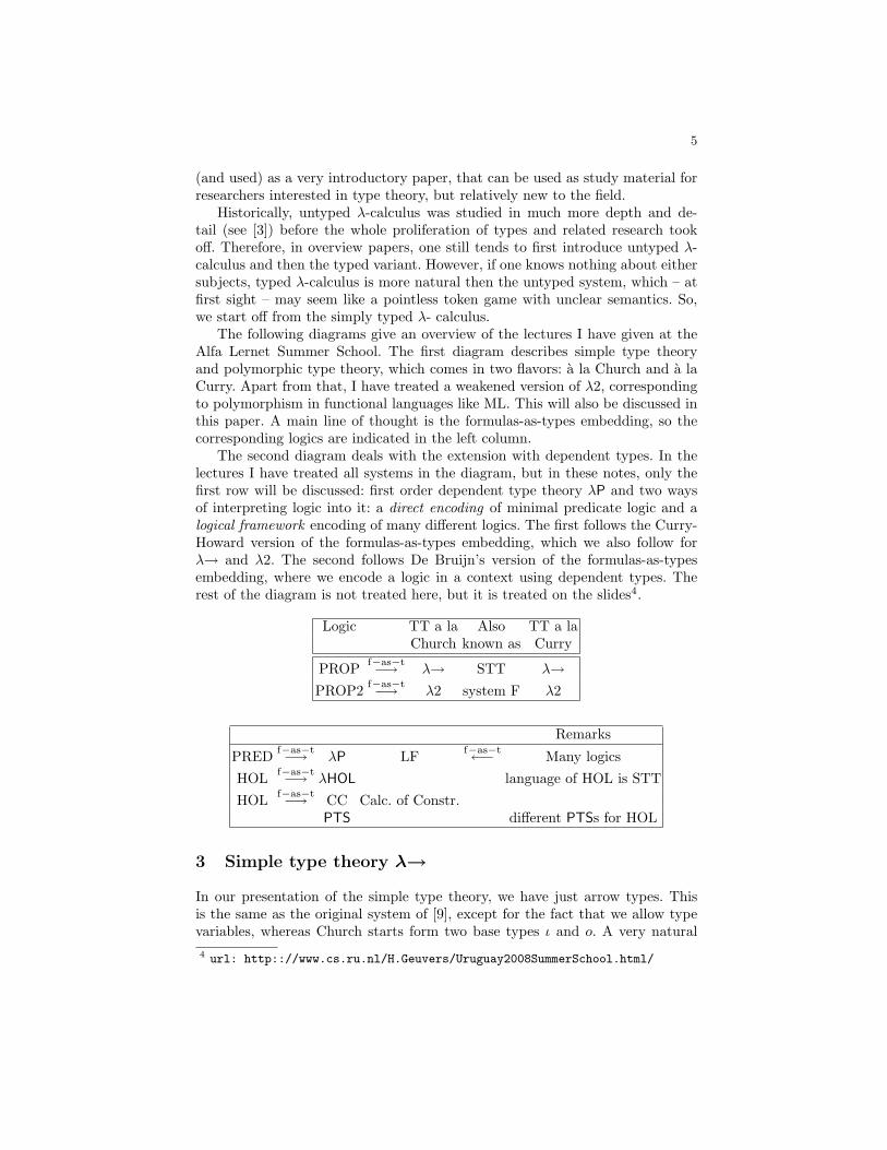
The following diagrams give an overview of the lectures I have given at theAlfa Lernet Summer School. The first diagram describes simple type theoryand polymorphic type theory, which comes in two flavors: a la Church and a laCurry. Apart from that, I have treated a weakened version of λ2, correspondingto polymorphism in functional languages like ML. This will also be discussed inthis paper. A main line of thought is the formulas-as-types embedding, so thecorresponding logics are indicated in the left column.

The second diagram deals with the extension with dependent types. In thelectures I have treated all systems in the diagram, but in these notes, only thefirst row will be discussed: first order dependent type theory λP and two waysof interpreting logic into it: a direct encoding of minimal predicate logic and alogical framework encoding of many different logics. The first follows the Curry-Howard version of the formulas-as-types embedding, which we also follow forλ→ and λ2. The second follows De Bruijn’s version of the formulas-as-typesembedding, where we encode a logic in a context using dependent types. Therest of the diagram is not treated here, but it is treated on the slides4.

Logic TT a la Also TT a laChurch known as Curry

PROP f−as−t−→ λ→ STT λ→PROP2 f−as−t−→ λ2 system F λ2

Remarks

PRED f−as−t−→ λP LF f−as−t←− Many logicsHOL f−as−t−→ λHOL language of HOL is STTHOL f−as−t−→ CC Calc. of Constr.

PTS different PTSs for HOL

3 Simple type theory λ→

In our presentation of the simple type theory, we have just arrow types. Thisis the same as the original system of [9], except for the fact that we allow typevariables, whereas Church starts form two base types ι and o. A very natural4 url: http:://www.cs.ru.nl/H.Geuvers/Uruguay2008SummerSchool.html/

6

extension is the one with product types and possibly other type constructions(like sum types, a unit type, . . . ). A good reference for the simple type theoryextended with product types is [27].

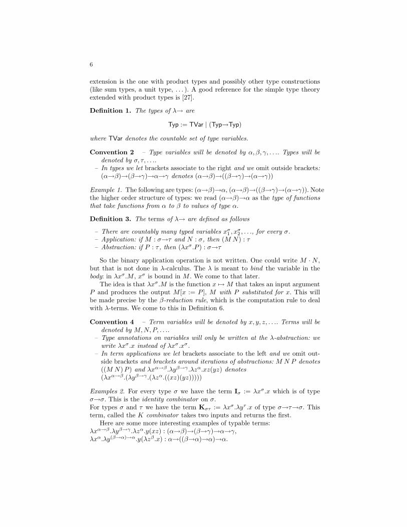
Definition 1. The types of λ→ are

Typ := TVar | (Typ→Typ)

where TVar denotes the countable set of type variables.

Convention 2 – Type variables will be denoted by α, β, γ, . . .. Types will bedenoted by σ, τ, . . ..

– In types we let brackets associate to the right and we omit outside brackets:(α→β)→(β→γ)→α→γ denotes (α→β)→((β→γ)→(α→γ))

Example 1. The following are types: (α→β)→α, (α→β)→((β→γ)→(α→γ)). Notethe higher order structure of types: we read (α→β)→α as the type of functionsthat take functions from α to β to values of type α.

Definition 3. The terms of λ→ are defined as follows

– There are countably many typed variables xσ1 , xσ2 , . . ., for every σ.

– Application: if M : σ→τ and N : σ, then (M N) : τ– Abstraction: if P : τ , then (λxσ.P ) : σ→τ

So the binary application operation is not written. One could write M · N ,but that is not done in λ-calculus. The λ is meant to bind the variable in thebody: in λxσ.M , xσ is bound in M . We come to that later.

The idea is that λxσ.M is the function x 7→M that takes an input argumentP and produces the output M [x := P ], M with P substituted for x. This willbe made precise by the β-reduction rule, which is the computation rule to dealwith λ-terms. We come to this in Definition 6.

Convention 4 – Term variables will be denoted by x, y, z, . . .. Terms will bedenoted by M,N,P, . . ..

– Type annotations on variables will only be written at the λ-abstraction: wewrite λxσ.x instead of λxσ.xσ.

– In term applications we let brackets associate to the left and we omit out-side brackets and brackets around iterations of abstractions: M N P denotes((M N)P ) and λxα→β .λyβ→γ .λzα.xz(yz) denotes(λxα→β .(λyβ→γ .(λzα.((xz)(yz)))))

Examples 2. For every type σ we have the term Iσ := λxσ.x which is of typeσ→σ. This is the identity combinator on σ.For types σ and τ we have the term Kστ := λxσ.λyτ .x of type σ→τ→σ. Thisterm, called the K combinator takes two inputs and returns the first.

Here are some more interesting examples of typable terms:λxα→β .λyβ→γ .λzα.y(xz) : (α→β)→(β→γ)→α→γ,λxα.λy(β→α)→α.y(λzβ .x) : α→((β→α)→α)→α.

7

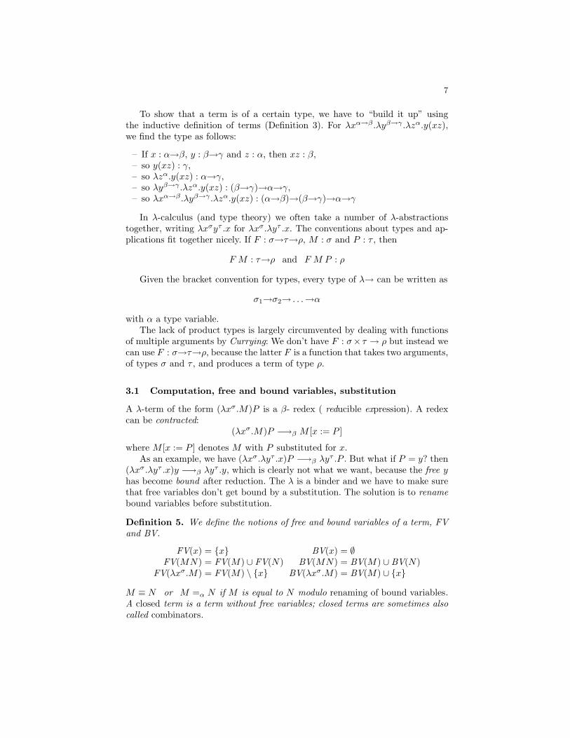
To show that a term is of a certain type, we have to “build it up” usingthe inductive definition of terms (Definition 3). For λxα→β .λyβ→γ .λzα.y(xz),we find the type as follows:

– If x : α→β, y : β→γ and z : α, then xz : β,– so y(xz) : γ,– so λzα.y(xz) : α→γ,– so λyβ→γ .λzα.y(xz) : (β→γ)→α→γ,– so λxα→β .λyβ→γ .λzα.y(xz) : (α→β)→(β→γ)→α→γ

In λ-calculus (and type theory) we often take a number of λ-abstractionstogether, writing λxσyτ .x for λxσ.λyτ .x. The conventions about types and ap-plications fit together nicely. If F : σ→τ→ρ, M : σ and P : τ , then

F M : τ→ρ and F M P : ρ

Given the bracket convention for types, every type of λ→ can be written as

σ1→σ2→ . . .→α

with α a type variable.The lack of product types is largely circumvented by dealing with functions

of multiple arguments by Currying: We don’t have F : σ× τ → ρ but instead wecan use F : σ→τ→ρ, because the latter F is a function that takes two arguments,of types σ and τ , and produces a term of type ρ.

3.1 Computation, free and bound variables, substitution

A λ-term of the form (λxσ.M)P is a β- redex ( reducible expression). A redexcan be contracted:

(λxσ.M)P −→β M [x := P ]

where M [x := P ] denotes M with P substituted for x.As an example, we have (λxσ.λyτ .x)P −→β λy

τ .P . But what if P = y? then(λxσ.λyτ .x)y −→β λy

τ .y, which is clearly not what we want, because the free yhas become bound after reduction. The λ is a binder and we have to make surethat free variables don’t get bound by a substitution. The solution is to renamebound variables before substitution.

Definition 5. We define the notions of free and bound variables of a term, FVand BV.

FV(x) = x BV(x) = ∅FV(MN) = FV(M) ∪ FV(N) BV(MN) = BV(M) ∪ BV(N)

FV(λxσ.M) = FV(M) \ x BV(λxσ.M) = BV(M) ∪ x

M ≡ N or M =α N if M is equal to N modulo renaming of bound variables.A closed term is a term without free variables; closed terms are sometimes alsocalled combinators.

8

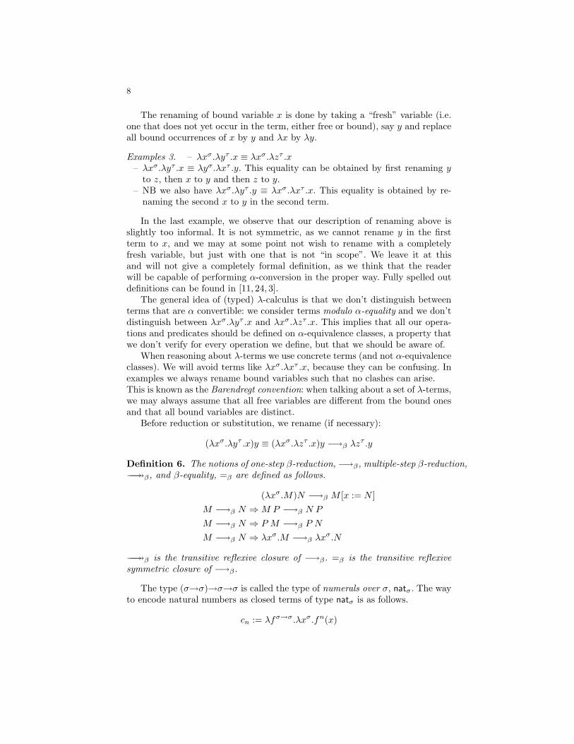
The renaming of bound variable x is done by taking a “fresh” variable (i.e.one that does not yet occur in the term, either free or bound), say y and replaceall bound occurrences of x by y and λx by λy.

Examples 3. – λxσ.λyτ .x ≡ λxσ.λzτ .x– λxσ.λyτ .x ≡ λyσ.λxτ .y. This equality can be obtained by first renaming y

to z, then x to y and then z to y.– NB we also have λxσ.λyτ .y ≡ λxσ.λxτ .x. This equality is obtained by re-

naming the second x to y in the second term.

In the last example, we observe that our description of renaming above isslightly too informal. It is not symmetric, as we cannot rename y in the firstterm to x, and we may at some point not wish to rename with a completelyfresh variable, but just with one that is not “in scope”. We leave it at thisand will not give a completely formal definition, as we think that the readerwill be capable of performing α-conversion in the proper way. Fully spelled outdefinitions can be found in [11, 24, 3].

The general idea of (typed) λ-calculus is that we don’t distinguish betweenterms that are α convertible: we consider terms modulo α-equality and we don’tdistinguish between λxσ.λyτ .x and λxσ.λzτ .x. This implies that all our opera-tions and predicates should be defined on α-equivalence classes, a property thatwe don’t verify for every operation we define, but that we should be aware of.

When reasoning about λ-terms we use concrete terms (and not α-equivalenceclasses). We will avoid terms like λxσ.λxτ .x, because they can be confusing. Inexamples we always rename bound variables such that no clashes can arise.This is known as the Barendregt convention: when talking about a set of λ-terms,we may always assume that all free variables are different from the bound onesand that all bound variables are distinct.

Before reduction or substitution, we rename (if necessary):

(λxσ.λyτ .x)y ≡ (λxσ.λzτ .x)y −→β λzτ .y

Definition 6. The notions of one-step β-reduction, −→β, multiple-step β-reduction,−→−→β, and β-equality, =β are defined as follows.

(λxσ.M)N −→β M [x := N ]M −→β N ⇒M P −→β N P

M −→β N ⇒ P M −→β P N

M −→β N ⇒ λxσ.M −→β λxσ.N

−→−→β is the transitive reflexive closure of −→β. =β is the transitive reflexivesymmetric closure of −→β.

The type (σ→σ)→σ→σ is called the type of numerals over σ, natσ. The wayto encode natural numbers as closed terms of type natσ is as follows.

cn := λfσ→σ.λxσ.fn(x)

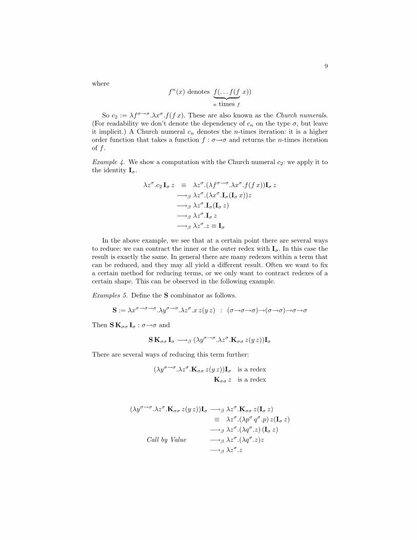
9

wherefn(x) denotes f(. . . f(f︸ ︷︷ ︸

n times f

x))

So c2 := λfσ→σ.λxσ.f(f x). These are also known as the Church numerals.(For readability we don’t denote the dependency of cn on the type σ, but leaveit implicit.) A Church numeral cn denotes the n-times iteration: it is a higherorder function that takes a function f : σ→σ and returns the n-times iterationof f .

Example 4. We show a computation with the Church numeral c2: we apply it tothe identity Iσ.

λzσ.c2 Iσ z ≡ λzσ.(λfσ→σ.λxσ.f(f x))Iσ z−→β λz

σ.(λxσ.Iσ(Iσ x))z−→β λz

σ.Iσ(Iσ z)−→β λz

σ.Iσ z

−→β λzσ.z ≡ Iσ

In the above example, we see that at a certain point there are several waysto reduce: we can contract the inner or the outer redex with Iσ. In this case theresult is exactly the same. In general there are many redexes within a term thatcan be reduced, and they may all yield a different result. Often we want to fixa certain method for reducing terms, or we only want to contract redexes of acertain shape. This can be observed in the following example.

Examples 5. Define the S combinator as follows.

S := λxσ→σ→σ.λyσ→σ.λzσ.x z(y z) : (σ→σ→σ)→(σ→σ)→σ→σ

Then S Kσσ Iσ : σ→σ and

S Kσσ Iσ −→β (λyσ→σ.λzσ.Kσσ z(y z))Iσ

There are several ways of reducing this term further:

(λyσ→σ.λzσ.Kσσ z(y z))Iσ is a redexKσσ z is a redex

(λyσ→σ.λzσ.Kσσ z(y z))Iσ −→β λzσ.Kσσ z(Iσ z)

≡ λzσ.(λpσ qσ.p) z(Iσ z)−→β λz

σ.(λqσ.z) (Iσ z)Call by Value −→β λz

σ.(λqσ.z)z−→β λz

σ.z

10

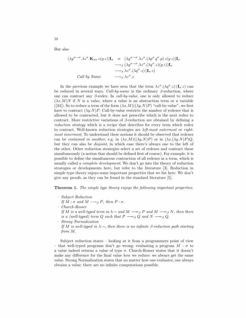
But also

(λyσ→σ.λzσ.Kσσ z(y z))Iσ ≡ (λyσ→σ.λzσ.(λpσ qσ.p) z(y z))Iσ−→β (λyσ→σ.λzσ.(λqσ.z)(y z))Iσ−→β λz

σ.(λqσ.z) (Iσ z)Call by Name −→β λz

σ.z

In the previous example we have seen that the term λzσ.(λqσ.z) (Iσ z) canbe reduced in several ways. Call-by-name is the ordinary β-reduction, whereone can contract any β-redex. In call-by-value, one is only allowed to reduce(λx.M)N if N is a value, where a value is an abstraction term or a variable([34]). So to reduce a term of the form (λx.M)((λy.N)P ) “call-by-value”, we firsthave to contract (λy.N)P . Call-by-value restricts the number of redexes that isallowed to be contracted, but it does not prescribe which is the next redex tocontract. More restrictive variations of β-reduction are obtained by defining areduction strategy which is a recipe that describes for every term which redexto contract. Well-known reduction strategies are left-most outermost or right-most innermost. To understand these notions it should be observed that redexescan be contained in another, e.g. in (λx.M)((λy.N)P ) or in (λx.(λy.N)P )Q,but they can also be disjoint, in which case there’s always one to the left ofthe other. Other reduction strategies select a set of redexes and contract thesesimultaneously (a notion that should be defined first of course). For example, it ispossible to define the simultaneous contraction of all redexes in a term, which isusually called a complete development. We don’t go into the theory of reductionstrategies or developments here, but refer to the literature [3]. Reduction insimple type theory enjoys some important properties that we list here. We don’tgive any proofs, as they can be found in the standard literature [5].

Theorem 1. The simple type theory enjoys the following important properties.

– Subject ReductionIf M : σ and M −→β P , then P : σ.

– Church-RosserIf M is a well-typed term in λ→ and M −→−→β P and M −→−→β N , then thereis a (well-typed) term Q such that P −→−→β Q and N −→−→β Q.

– Strong NormalizationIf M is well-typed in λ→, then there is no infinite β-reduction path startingfrom M .

Subject reduction states – looking at it from a programmers point of view– that well-typed programs don’t go wrong: evaluating a program M : σ toa value indeed returns a value of type σ. Church-Rosser states that it doesn’tmake any difference for the final value how we reduce: we always get the samevalue. Strong Normalization states that no matter how one evaluates, one alwaysobtains a value: there are no infinite computations possible.

11

3.2 Simple type theory presented with derivation rules

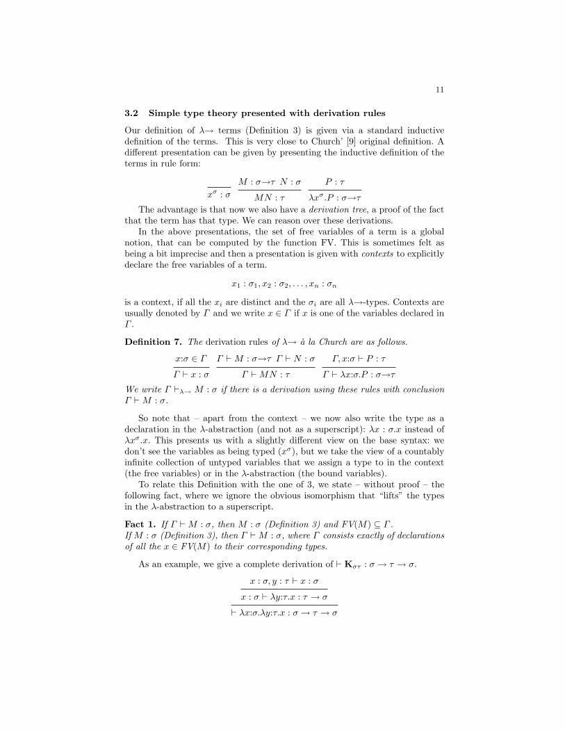
Our definition of λ→ terms (Definition 3) is given via a standard inductivedefinition of the terms. This is very close to Church’ [9] original definition. Adifferent presentation can be given by presenting the inductive definition of theterms in rule form:

xσ : σM : σ→τ N : σ

MN : τ

P : τ

λxσ.P : σ→τThe advantage is that now we also have a derivation tree, a proof of the fact

that the term has that type. We can reason over these derivations.In the above presentations, the set of free variables of a term is a global

notion, that can be computed by the function FV. This is sometimes felt asbeing a bit imprecise and then a presentation is given with contexts to explicitlydeclare the free variables of a term.

x1 : σ1, x2 : σ2, . . . , xn : σn

is a context, if all the xi are distinct and the σi are all λ→-types. Contexts areusually denoted by Γ and we write x ∈ Γ if x is one of the variables declared inΓ .

Definition 7. The derivation rules of λ→ a la Church are as follows.

x:σ ∈ Γ

Γ ` x : σ

Γ `M : σ→τ Γ ` N : σ

Γ `MN : τ

Γ, x:σ ` P : τ

Γ ` λx:σ.P : σ→τWe write Γ `λ→ M : σ if there is a derivation using these rules with conclusionΓ `M : σ.

So note that – apart from the context – we now also write the type as adeclaration in the λ-abstraction (and not as a superscript): λx : σ.x instead ofλxσ.x. This presents us with a slightly different view on the base syntax: wedon’t see the variables as being typed (xσ), but we take the view of a countablyinfinite collection of untyped variables that we assign a type to in the context(the free variables) or in the λ-abstraction (the bound variables).

To relate this Definition with the one of 3, we state – without proof – thefollowing fact, where we ignore the obvious isomorphism that “lifts” the typesin the λ-abstraction to a superscript.

Fact 1. If Γ `M : σ, then M : σ (Definition 3) and FV(M) ⊆ Γ .If M : σ (Definition 3), then Γ `M : σ, where Γ consists exactly of declarationsof all the x ∈ FV(M) to their corresponding types.

As an example, we give a complete derivation of ` Kστ : σ → τ → σ.

x : σ, y : τ ` x : σ

x : σ ` λy:τ.x : τ → σ

` λx:σ.λy:τ.x : σ → τ → σ

12

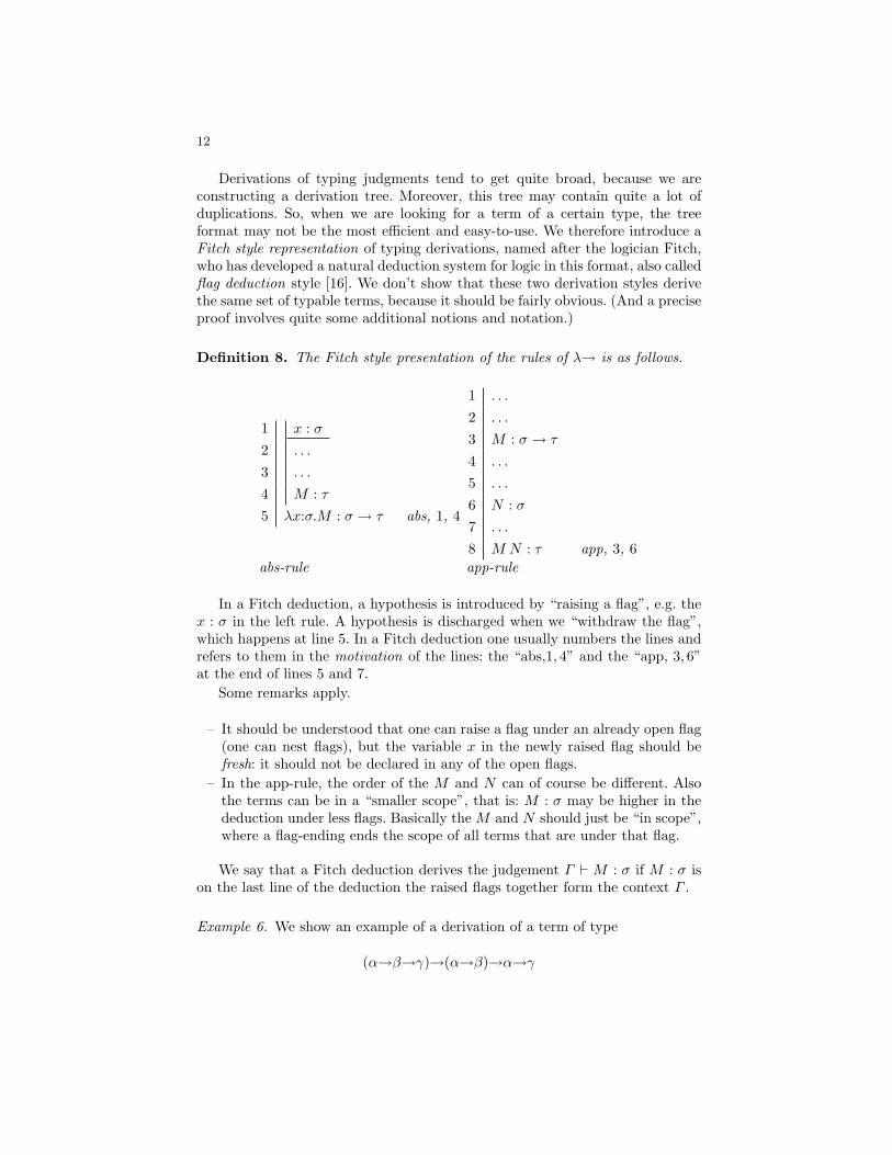
Derivations of typing judgments tend to get quite broad, because we areconstructing a derivation tree. Moreover, this tree may contain quite a lot ofduplications. So, when we are looking for a term of a certain type, the treeformat may not be the most efficient and easy-to-use. We therefore introduce aFitch style representation of typing derivations, named after the logician Fitch,who has developed a natural deduction system for logic in this format, also calledflag deduction style [16]. We don’t show that these two derivation styles derivethe same set of typable terms, because it should be fairly obvious. (And a preciseproof involves quite some additional notions and notation.)

Definition 8. The Fitch style presentation of the rules of λ→ is as follows.

1 x : σ2 . . .

3 . . .

4 M : τ5 λx:σ.M : σ → τ abs, 1, 4

1 . . .

2 . . .

3 M : σ → τ

4 . . .

5 . . .

6 N : σ7 . . .

8 M N : τ app, 3, 6abs-rule app-rule

In a Fitch deduction, a hypothesis is introduced by “raising a flag”, e.g. thex : σ in the left rule. A hypothesis is discharged when we “withdraw the flag”,which happens at line 5. In a Fitch deduction one usually numbers the lines andrefers to them in the motivation of the lines: the “abs,1, 4” and the “app, 3, 6”at the end of lines 5 and 7.

Some remarks apply.

– It should be understood that one can raise a flag under an already open flag(one can nest flags), but the variable x in the newly raised flag should befresh: it should not be declared in any of the open flags.

– In the app-rule, the order of the M and N can of course be different. Alsothe terms can be in a “smaller scope”, that is: M : σ may be higher in thededuction under less flags. Basically the M and N should just be “in scope”,where a flag-ending ends the scope of all terms that are under that flag.

We say that a Fitch deduction derives the judgement Γ ` M : σ if M : σ ison the last line of the deduction the raised flags together form the context Γ .

Example 6. We show an example of a derivation of a term of type

(α→β→γ)→(α→β)→α→γ

13

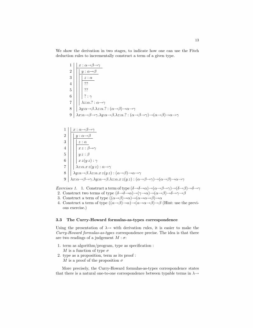
We show the derivation in two stages, to indicate how one can use the Fitchdeduction rules to incrementally construct a term of a given type.

1 x : α→β→γ2 y : α→β3 z : α4 ??5 ??6 ? : γ7 λz:α.? : α→γ8 λy:α→β.λz:α.? : (α→β)→α→γ9 λx:α→β→γ.λy:α→β.λz:α.? : (α→β→γ)→(α→β)→α→γ

1 x : α→β→γ2 y : α→β3 z : α4 x z : β→γ5 y z : β6 x z(y z) : γ7 λz:α.x z(y z) : α→γ8 λy:α→β.λz:α.x z(y z) : (α→β)→α→γ9 λx:α→β→γ.λy:α→β.λz:α.x z(y z) : (α→β→γ)→(α→β)→α→γ

Exercises 1. 1. Construct a term of type (δ→δ→α)→(α→β→γ)→(δ→β)→δ→γ2. Construct two terms of type (δ→δ→α)→(γ→α)→(α→β)→δ→γ→β3. Construct a term of type ((α→β)→α)→(α→α→β)→α4. Construct a term of type ((α→β)→α)→(α→α→β)→β (Hint: use the previ-

ous exercise.)

3.3 The Curry-Howard formulas-as-types correspondence

Using the presentation of λ→ with derivation rules, it is easier to make theCurry-Howard formulas-as-types correspondence precise. The idea is that thereare two readings of a judgement M : σ:

1. term as algorithm/program, type as specification :M is a function of type σ

2. type as a proposition, term as its proof :M is a proof of the proposition σ

More precisely, the Curry-Howard formulas-as-types correspondence statesthat there is a natural one-to-one correspondence between typable terms in λ→

14

and derivations in minimal proposition logic. Looking at it from the logical pointof view: the judgement x1 : τ1, x2 : τ2, . . . , xn : τn ` M : σ can be read as M isa proof of σ from the assumptions τ1, τ2, . . . , τn.

Definition 9. The system of minimal proposition logic PROP consists of

– implicational propositions, generated by the following abstract syntax:

prop ::= PropVar|(prop→prop)

– derivation rules (∆ is a set of propositions, σ and τ are propositions)

σ→τ σ→-E

τ

[σ]j...τ

[j]→-Iσ→τ

We write ∆ `PROP σ if there is a derivation using these rules with conclusionσ and non-discharged assumptions in ∆.

Note the difference between a context, which is basically a list, and a set ofassumptions. Logic (certainly in natural deduction) is usually presented using aset of assumptions, but there is no special reason for not letting the assumptionsbe a list, or a multi-set.

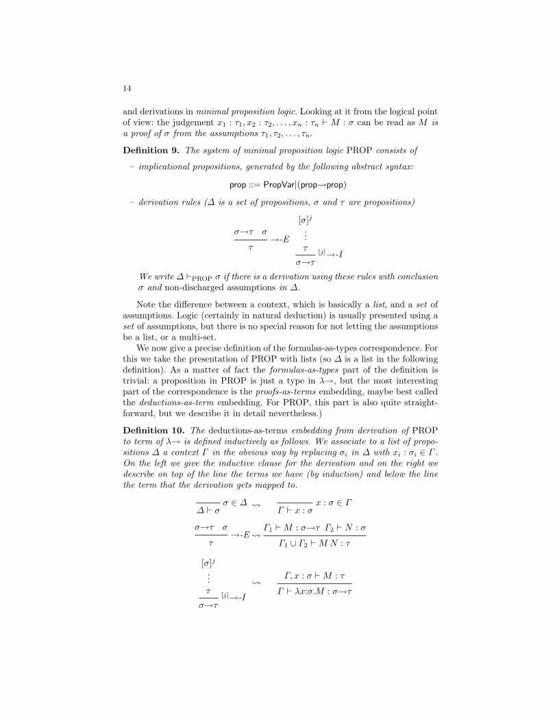
We now give a precise definition of the formulas-as-types correspondence. Forthis we take the presentation of PROP with lists (so ∆ is a list in the followingdefinition). As a matter of fact the formulas-as-types part of the definition istrivial: a proposition in PROP is just a type in λ→, but the most interestingpart of the correspondence is the proofs-as-terms embedding, maybe best calledthe deductions-as-term embedding. For PROP, this part is also quite straight-forward, but we describe it in detail nevertheless.)

Definition 10. The deductions-as-terms embedding from derivation of PROPto term of λ→ is defined inductively as follows. We associate to a list of propo-sitions ∆ a context Γ in the obvious way by replacing σi in ∆ with xi : σi ∈ Γ .On the left we give the inductive clause for the derivation and on the right wedescribe on top of the line the terms we have (by induction) and below the linethe term that the derivation gets mapped to.

σ ∈ ∆∆ ` σ x : σ ∈ Γ

Γ ` x : σ

σ→τ σ→-E

τ Γ1 `M : σ→τ Γ2 ` N : σ

Γ1 ∪ Γ2 `M N : τ

[σ]j...τ

[j]→-Iσ→τ

Γ, x : σ `M : τ

Γ ` λx:σ.M : σ→τ

15

We denote this embedding by −, so if D is a derivation from PROP, D is aλ→-term.

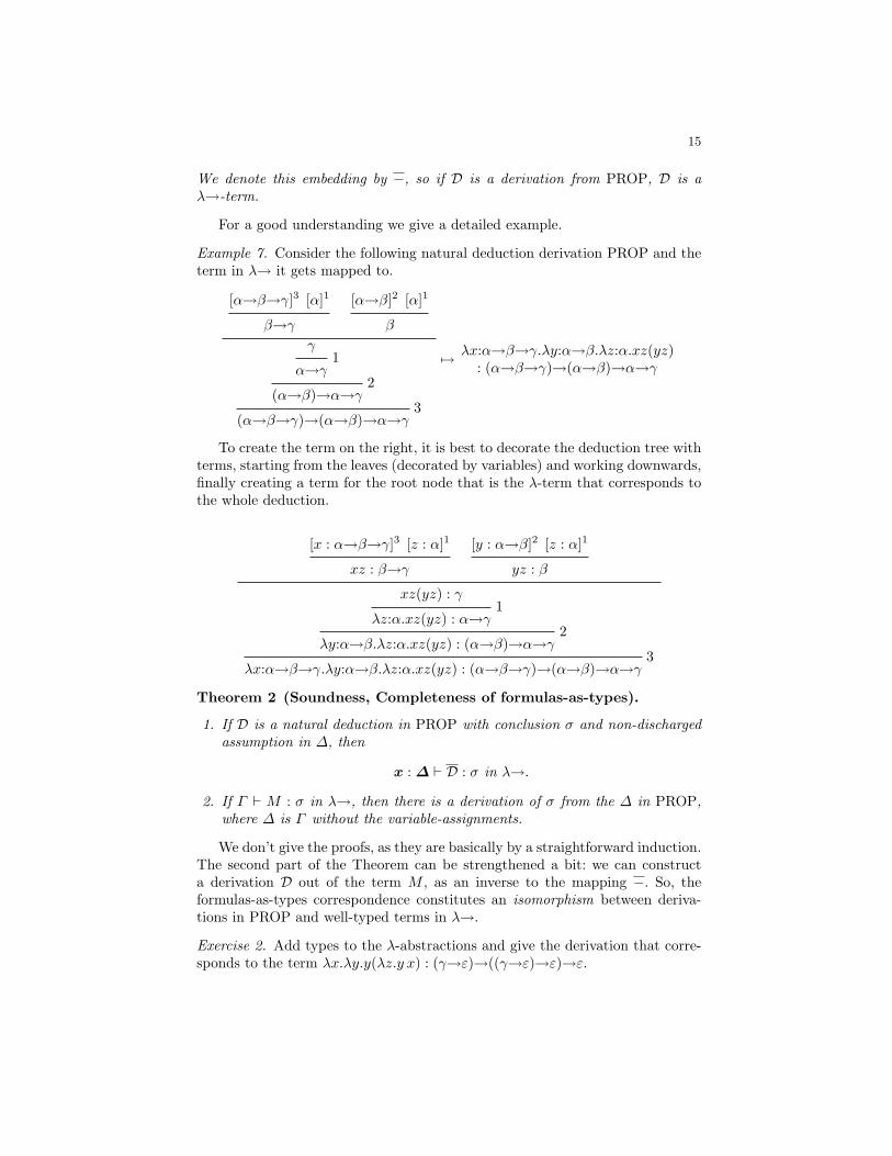
For a good understanding we give a detailed example.

Example 7. Consider the following natural deduction derivation PROP and theterm in λ→ it gets mapped to.

[α→β→γ]3 [α]1

β→γ

[α→β]2 [α]1

β

γ1

α→γ2

(α→β)→α→γ3

(α→β→γ)→(α→β)→α→γ

7→ λx:α→β→γ.λy:α→β.λz:α.xz(yz): (α→β→γ)→(α→β)→α→γ

To create the term on the right, it is best to decorate the deduction tree withterms, starting from the leaves (decorated by variables) and working downwards,finally creating a term for the root node that is the λ-term that corresponds tothe whole deduction.

[x : α→β→γ]3 [z : α]1

xz : β→γ

[y : α→β]2 [z : α]1

yz : β

xz(yz) : γ1

λz:α.xz(yz) : α→γ2

λy:α→β.λz:α.xz(yz) : (α→β)→α→γ3

λx:α→β→γ.λy:α→β.λz:α.xz(yz) : (α→β→γ)→(α→β)→α→γ

Theorem 2 (Soundness, Completeness of formulas-as-types).

1. If D is a natural deduction in PROP with conclusion σ and non-dischargedassumption in ∆, then

x : ∆ ` D : σ in λ→.

2. If Γ ` M : σ in λ→, then there is a derivation of σ from the ∆ in PROP,where ∆ is Γ without the variable-assignments.

We don’t give the proofs, as they are basically by a straightforward induction.The second part of the Theorem can be strengthened a bit: we can constructa derivation D out of the term M , as an inverse to the mapping −. So, theformulas-as-types correspondence constitutes an isomorphism between deriva-tions in PROP and well-typed terms in λ→.

Exercise 2. Add types to the λ-abstractions and give the derivation that corre-sponds to the term λx.λy.y(λz.y x) : (γ→ε)→((γ→ε)→ε)→ε.

16

In the λ-calculus we have a notion of computation, given by β-reduction:(λx:σ.M)P −→β M [x := P ]. Apart from that, there is also a notion of η-reduction: λx:σ.M x −→η M if x /∈ FV(M). The idea of considering these termsas equal is quite natural, because they behave exactly the same as functions:(λx:σ.M x)P −→β M P . In a typed setting, it is very natural to consider therule in the opposite direction, because then one can make sure that every term ofa function type has a normal form that is a λ-abstraction. Of course this requiresa proviso to prevent an infinite η-reduction of the form x −→η λy:σ.x y −→η

λy:σ.(λz:σ.x z)y . . .In natural deduction we also have a notion of computation: cut-elimination or

detour-elimination. If one introduces a connective and then immediately elim-inates it again, this is called a cut or a detour. A cut is actually a rule inthe sequent calculus representation of logic and the cut-elimination theorem insequent calculus states that the cut-rule is derivable and thus superfluous. Innatural deduction, we can eliminate detours, which are often also called cuts, aterminology that we will also use here.

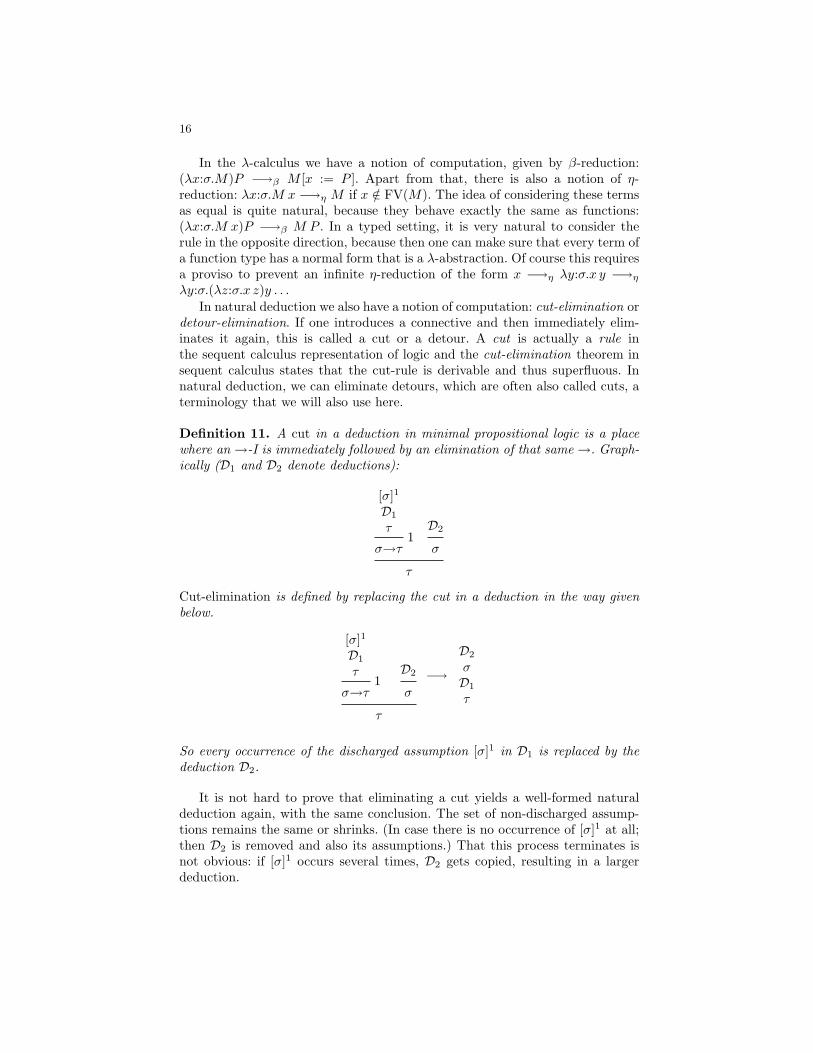
Definition 11. A cut in a deduction in minimal propositional logic is a placewhere an →-I is immediately followed by an elimination of that same →. Graph-ically (D1 and D2 denote deductions):

[σ]1

D1

τ1

σ→τ

D2

σ

τ

Cut-elimination is defined by replacing the cut in a deduction in the way givenbelow.

[σ]1

D1

τ1

σ→τ

D2

σ

τ

−→

D2

σD1

τ

So every occurrence of the discharged assumption [σ]1 in D1 is replaced by thededuction D2.

It is not hard to prove that eliminating a cut yields a well-formed naturaldeduction again, with the same conclusion. The set of non-discharged assump-tions remains the same or shrinks. (In case there is no occurrence of [σ]1 at all;then D2 is removed and also its assumptions.) That this process terminates isnot obvious: if [σ]1 occurs several times, D2 gets copied, resulting in a largerdeduction.

17

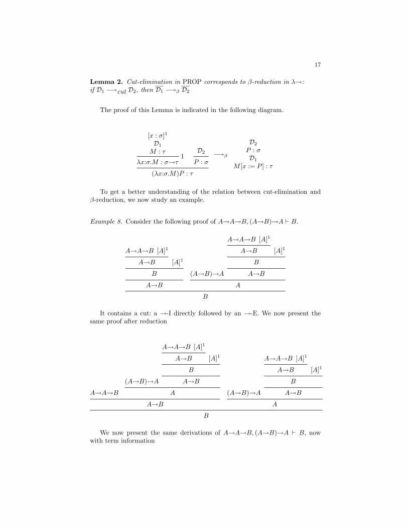
Lemma 2. Cut-elimination in PROP corresponds to β-reduction in λ→:if D1 −→cut D2, then D1 −→β D2

The proof of this Lemma is indicated in the following diagram.

[x : σ]1

D1

M : τ1

λx:σ.M : σ→τ

D2

P : σ

(λx:σ.M)P : τ

−→β

D2

P : σD1

M [x := P ] : τ

To get a better understanding of the relation between cut-elimination andβ-reduction, we now study an example.

Example 8. Consider the following proof of A→A→B, (A→B)→A ` B.

A→A→B [A]1

A→B [A]1

B

A→B

(A→B)→A

A→A→B [A]1

A→B [A]1

B

A→B

A

B

It contains a cut: a →-I directly followed by an →-E. We now present thesame proof after reduction

A→A→B

(A→B)→A

A→A→B [A]1

A→B [A]1

B

A→B

A

A→B

(A→B)→A

A→A→B [A]1

A→B [A]1

B

A→B

A

B

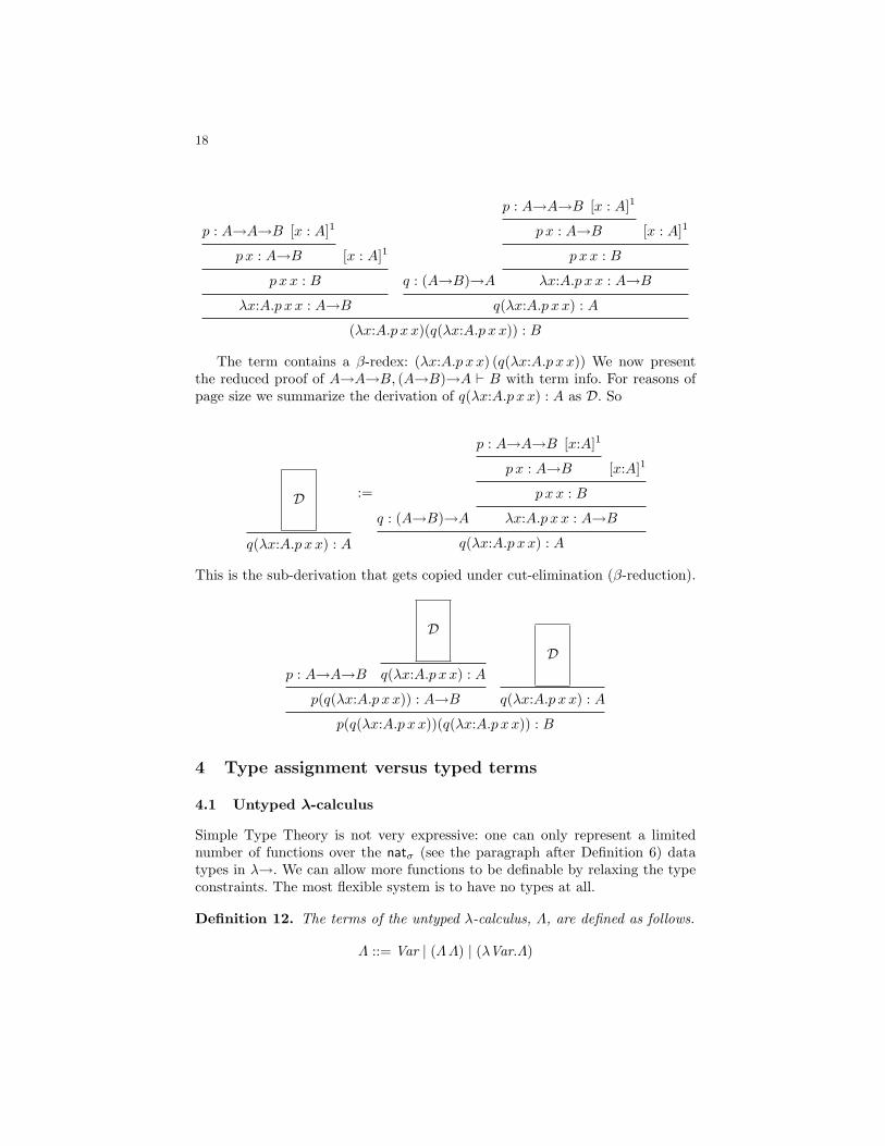
We now present the same derivations of A→A→B, (A→B)→A ` B, nowwith term information

18

p : A→A→B [x : A]1

p x : A→B [x : A]1

p xx : B

λx:A.p xx : A→B

q : (A→B)→A

p : A→A→B [x : A]1

p x : A→B [x : A]1

p xx : B

λx:A.p xx : A→B

q(λx:A.p xx) : A

(λx:A.p xx)(q(λx:A.p xx)) : B

The term contains a β-redex: (λx:A.p xx) (q(λx:A.p xx)) We now presentthe reduced proof of A→A→B, (A→B)→A ` B with term info. For reasons ofpage size we summarize the derivation of q(λx:A.p xx) : A as D. So

D

q(λx:A.p xx) : A

:=

q : (A→B)→A

p : A→A→B [x:A]1

p x : A→B [x:A]1

p xx : B

λx:A.p xx : A→B

q(λx:A.p xx) : A

This is the sub-derivation that gets copied under cut-elimination (β-reduction).

p : A→A→B

D

q(λx:A.p xx) : A

p(q(λx:A.p xx)) : A→B

D

q(λx:A.p xx) : A

p(q(λx:A.p xx))(q(λx:A.p xx)) : B

4 Type assignment versus typed terms

4.1 Untyped λ-calculus

Simple Type Theory is not very expressive: one can only represent a limitednumber of functions over the natσ (see the paragraph after Definition 6) datatypes in λ→. We can allow more functions to be definable by relaxing the typeconstraints. The most flexible system is to have no types at all.

Definition 12. The terms of the untyped λ-calculus, Λ, are defined as follows.

Λ ::= Var | (ΛΛ) | (λVar.Λ)

19

Examples are the well-known combinators that we have already seen in atyped fashion: K := λx y.x, S := λx y z.x z(y z). But we can now do more: hereare some well-known untyped λ-terms ω := λx.x x, Ω := ω ω. The notions ofβ-reduction and β-equality generalize from the simple typed case, so we don’trepeat it here. An interesting aspect is that we can now have infinite reduc-tions. (Which is impossible in λ→, as that system is Strongly Normalizing.) Thesimplest infinite reduction is the following loop:

Ω −→β Ω

A term that doesn’t loop but whose reduction path contains infinitely manydifferent terms is obtained by putting ω3 := λx.x xx, Ω3 := ω3ω3. Then:

Ω3 −→β ω3 ω3 ω3 −→β ω3 ω3 ω3 ω3 −→β . . .

The untyped λ-calculus was defined by Church [9] and proposed as a systemto capture the notion of mechanic computation, for which Turing proposed thenotion of Turing machine. An important property of the untyped λ-calculus isthat it is Turing complete, which was proved by Turing in 1936, see [13]. Thepower of Λ lies in the fact that you can solve recursive equations.

A recursive equation is a question of the following kind:

– Is there a term M such that

M x =β xM x?

– Is there a term M such that

M x =β if (Zerox) then 1 else Multx (M (Predx))?

So, we have two expressions on either side of the =β sign, both containing anunknown M and we want to know whether a solution for M exists.

The answer is: yes, if we can rewrite the equation to one of the form

M =β . . .M . . . (1)

Note that this is possible for the equations written above. For example the firstequation is solved by a term M that satisfies M =β λx.xM x.

That we can solve equation of the form (1) is because every term in theλ-calculus has a fixed point. Even more: we have a fixed point combinator.

Definition 13. – The term M is a fixed point of the term P if P M =β M .– The term Y is a fixed point combinator if for every term P , Y P is a fixed

point of P , that is ifP (Y P ) =β Y P.

In the λ-calculus we have various fixed point combinators, of which the Y -combinator is the most well-known one: Y := λf.(λx.f(xx))(λx.f(xx)).

20

Exercise 3. Verify that the Y as defined above is a fixed point combinator:P (Y P ) =β Y P for every λ-term P .Verify that Θ := (λx y.y(xx y))(λx y.y(xx y)) is also a fixed point combinatorthat is even reducing: ΘP −→−→β P (ΘP ) for every λ-term P .

The existence of fixed-points is the key to the power of the λ-calculus. Butwe also need natural numbers and booleans to be able to write programs. InSection 3 we have already seen the Church numerals:

cn := λf.λx.fn(x)

wherefn(x) denotes f(. . . f(f︸ ︷︷ ︸

n times f

x))

The successor is easy to define for these numerals: Suc := λn.λf x.f(n f x).Addition can also be defined quite easily, but if we are lazy we can also use thefixed-point combinator. We want to solve

Addnm := if(Zeron) thenm else Add (Predn)m)

where Pred is the predecessor function, Zero is a test for zero and if . . . then . . . elseis a case distinction on booleans. The booleans can be defined by

true := λx y.x

false := λx y.y

if b thenP elseQ := b P Q.

Exercise 4. 1. Verify that the booleans behave as expected:if true thenP elseQ =β P and if false thenP elseQ =β Q.

2. Define a test-for-zero Zero on the Church numerals :Zero c0 =β true andZero cn+1 =β false. (Defining the predecessor is remarkably tricky!)

Apart from the natural numbers and booleans, it is not difficult to findencodings of other data, like lists and trees. Given the expressive power of theuntyped λ-calculus and the limited expressive power of λ→, one may wonder whywe want types. There are various good reasons for that, most of which apply tothe the “typed versus untyped programming languages” issue in general.

Types give a (partial) specification. Types tell the programmer – and a personreading the program — what a program (λ-term) does, to a certain extent. Typesonly give a very partial specification, like f : IN→ IN, but depending on the typesystem, this information can be enriched, for example: f : Πn : IN.∃m : IN.m >n, stating that f is a program that takes a number n and returns an m thatis larger than n. In the Chapter by Bove and Dybjer, one can find examples ofthat type and we will also come back to this theme in this Chapter in Section 6.

21

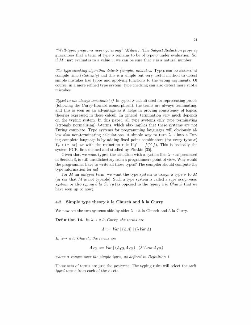
“Well-typed programs never go wrong” (Milner). The Subject Reduction propertyguarantees that a term of type σ remains to be of type σ under evaluation. So,if M : nat evaluates to a value v, we can be sure that v is a natural number.

The type checking algorithm detects (simple) mistakes. Types can be checked atcompile time (statically) and this is a simple but very useful method to detectsimple mistakes like typos and applying functions to the wrong arguments. Ofcourse, in a more refined type system, type checking can also detect more subtlemistakes.

Typed terms always terminate(?) In typed λ-calculi used for representing proofs(following the Curry-Howard isomorphism), the terms are always terminating,and this is seen as an advantage as it helps in proving consistency of logicaltheories expressed in these calculi. In general, termination very much dependson the typing system. In this paper, all type systems only type terminating(strongly normalizing) λ-terms, which also implies that these systems are notTuring complete. Type systems for programming languages will obviously al-low also non-terminating calculations. A simple way to turn λ→ into a Tur-ing complete language is by adding fixed point combinators (for every type σ)Yσ : (σ→σ)→σ with the reduction rule Y f → f(Y f). This is basically thesystem PCF, first defined and studied by Plotkin [35].

Given that we want types, the situation with a system like λ→ as presentedin Section 3, is still unsatisfactory from a programmers point of view. Why wouldthe programmer have to write all those types? The compiler should compute thetype information for us!

For M an untyped term, we want the type system to assign a type σ to M(or say that M is not typable). Such a type system is called a type assignmentsystem, or also typing a la Curry (as opposed to the typing a la Church that wehave seen up to now).

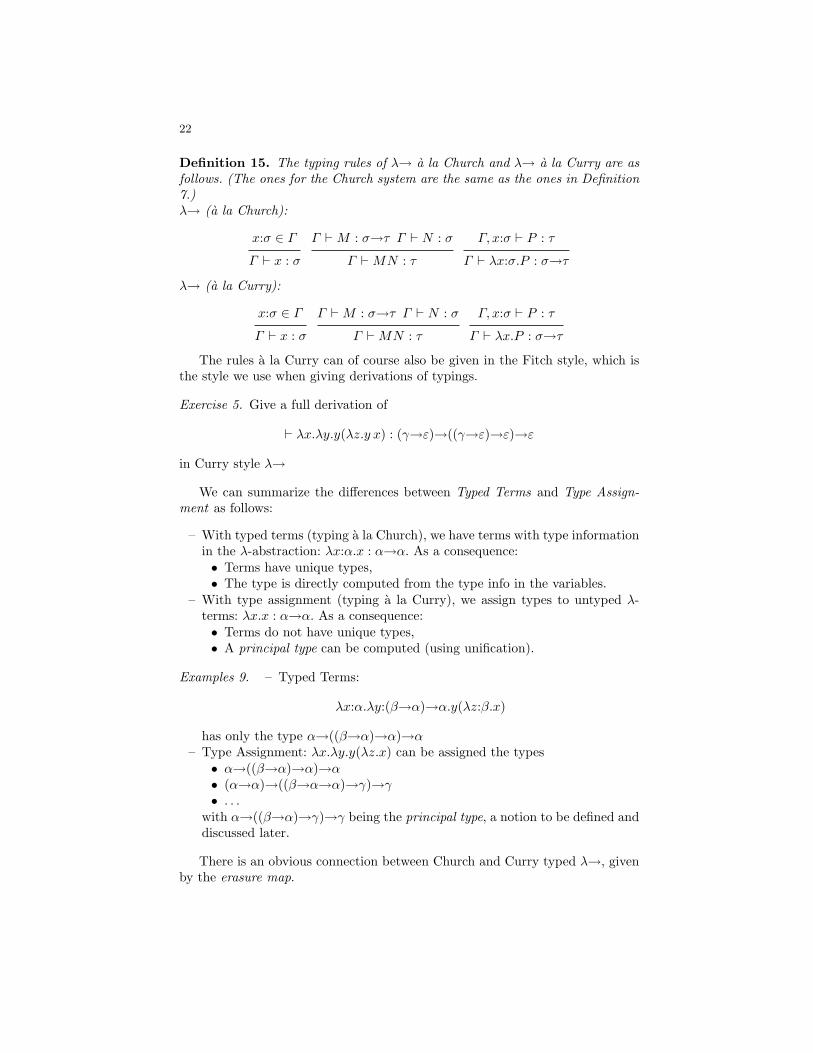
4.2 Simple type theory a la Church and a la Curry

We now set the two systems side-by-side: λ→ a la Church and a la Curry.

Definition 14. In λ→ a la Curry, the terms are

Λ ::= Var | (ΛΛ) | (λVar.Λ)

In λ→ a la Church, the terms are

ΛCh ::= Var | (ΛCh ΛCh) | (λVar:σ.ΛCh)

where σ ranges over the simple types, as defined in Definition 1.

These sets of terms are just the preterms. The typing rules will select the well-typed terms from each of these sets.

22

Definition 15. The typing rules of λ→ a la Church and λ→ a la Curry are asfollows. (The ones for the Church system are the same as the ones in Definition7.)λ→ (a la Church):

x:σ ∈ Γ

Γ ` x : σ

Γ `M : σ→τ Γ ` N : σ

Γ `MN : τ

Γ, x:σ ` P : τ

Γ ` λx:σ.P : σ→τ

λ→ (a la Curry):

x:σ ∈ Γ

Γ ` x : σ

Γ `M : σ→τ Γ ` N : σ

Γ `MN : τ

Γ, x:σ ` P : τ

Γ ` λx.P : σ→τ

The rules a la Curry can of course also be given in the Fitch style, which isthe style we use when giving derivations of typings.

Exercise 5. Give a full derivation of

` λx.λy.y(λz.y x) : (γ→ε)→((γ→ε)→ε)→ε

in Curry style λ→

We can summarize the differences between Typed Terms and Type Assign-ment as follows:

– With typed terms (typing a la Church), we have terms with type informationin the λ-abstraction: λx:α.x : α→α. As a consequence:• Terms have unique types,• The type is directly computed from the type info in the variables.

– With type assignment (typing a la Curry), we assign types to untyped λ-terms: λx.x : α→α. As a consequence:• Terms do not have unique types,• A principal type can be computed (using unification).

Examples 9. – Typed Terms:

λx:α.λy:(β→α)→α.y(λz:β.x)

has only the type α→((β→α)→α)→α– Type Assignment: λx.λy.y(λz.x) can be assigned the types• α→((β→α)→α)→α• (α→α)→((β→α→α)→γ)→γ• . . .

with α→((β→α)→γ)→γ being the principal type, a notion to be defined anddiscussed later.

There is an obvious connection between Church and Curry typed λ→, givenby the erasure map.

23

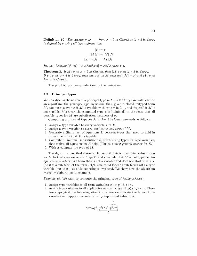
Definition 16. The erasure map | − | from λ→ a la Church to λ→ a la Curryis defined by erasing all type information:

|x| := x

|M N | := |M | |N ||λx : σ.M | := λx.|M |

So, e.g. |λx:α.λy:(β→α)→α.y(λz:β.x))| = λx.λy.y(λz.x)).

Theorem 3. If M : σ in λ→ a la Church, then |M | : σ in λ→ a la Curry.If P : σ in λ→ a la Curry, then there is an M such that |M | ≡ P and M : σ inλ→ a la Church.

The proof is by an easy induction on the derivation.

4.3 Principal types

We now discuss the notion of a principal type in λ→ a la Curry. We will describean algorithm, the principal type algorithm, that, given a closed untyped termM , computes a type σ if M is typable with type σ in λ→, and “reject” if M isnot typable. Moreover, the computed type σ is “minimal” in the sense that allpossible types for M are substitution instances of σ.

Computing a principal type for M in λ→ a la Curry proceeds as follows:

1. Assign a type variable to every variable x in M .2. Assign a type variable to every applicative sub-term of M .3. Generate a (finite) set of equations E between types that need to hold in

order to ensure that M is typable.4. Compute a “minimal substitution” S, substituting types for type variables,

that makes all equations in E hold. (This is a most general unifier for E.)5. With S compute the type of M .

The algorithm described above can fail only if their is no unifying substitutionfor E. In that case we return “reject” and conclude that M is not typable. Anapplicative sub-term is a term that is not a variable and does not start with a λ.(So it is a sub-term of the form P Q). One could label all sub-terms with a typevariable, but that just adds superfluous overhead. We show how the algorithmworks by elaborating an example.

Example 10. We want to compute the principal type of λx.λy.y(λz.yx).

1. Assign type variables to all term variables: x : α, y : β, z : γ.2. Assign type variables to all applicative sub-terms: y x : δ, y(λz.y x) : ε. These

two steps yield the following situation, where we indicate the types of thevariables and applicative sub-terms by super- and subscripts.

λxα.λyβ . yβ(λzγ .

δ︷ ︸︸ ︷yβxα)︸ ︷︷ ︸

ε

24

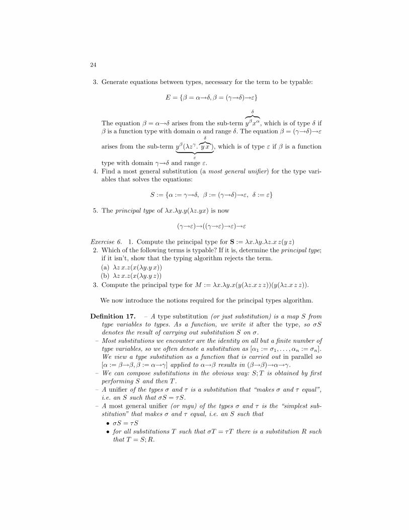
3. Generate equations between types, necessary for the term to be typable:

E = β = α→δ, β = (γ→δ)→ε

The equation β = α→δ arises from the sub-term

δ︷ ︸︸ ︷yβxα, which is of type δ if

β is a function type with domain α and range δ. The equation β = (γ→δ)→ε

arises from the sub-term yβ(λzγ .δ︷︸︸︷y x )︸ ︷︷ ︸

ε

, which is of type ε if β is a function

type with domain γ→δ and range ε.4. Find a most general substitution (a most general unifier) for the type vari-

ables that solves the equations:

S := α := γ→δ, β := (γ→δ)→ε, δ := ε

5. The principal type of λx.λy.y(λz.yx) is now

(γ→ε)→((γ→ε)→ε)→ε

Exercise 6. 1. Compute the principal type for S := λx.λy.λz.x z(y z)2. Which of the following terms is typable? If it is, determine the principal type;

if it isn’t, show that the typing algorithm rejects the term.(a) λz x.z(x(λy.y x))(b) λz x.z(x(λy.y z))

3. Compute the principal type for M := λx.λy.x(y(λz.x z z))(y(λz.x z z)).

We now introduce the notions required for the principal types algorithm.

Definition 17. – A type substitution (or just substitution) is a map S fromtype variables to types. As a function, we write it after the type, so σSdenotes the result of carrying out substitution S on σ.

– Most substitutions we encounter are the identity on all but a finite number oftype variables, so we often denote a substitution as [α1 := σ1, . . . , αn := σn].We view a type substitution as a function that is carried out in parallel so[α := β→β, β := α→γ] applied to α→β results in (β→β)→α→γ.

– We can compose substitutions in the obvious way: S;T is obtained by firstperforming S and then T .

– A unifier of the types σ and τ is a substitution that “makes σ and τ equal”,i.e. an S such that σS = τS.

– A most general unifier (or mgu) of the types σ and τ is the “simplest sub-stitution” that makes σ and τ equal, i.e. an S such that• σS = τS

• for all substitutions T such that σT = τT there is a substitution R suchthat T = S;R.

25

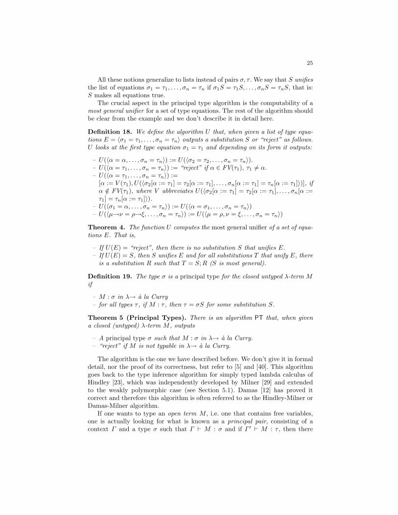
All these notions generalize to lists instead of pairs σ, τ . We say that S unifiesthe list of equations σ1 = τ1, . . . , σn = τn if σ1S = τ1S, . . . , σnS = τnS, that is:S makes all equations true.

The crucial aspect in the principal type algorithm is the computability of amost general unifier for a set of type equations. The rest of the algorithm shouldbe clear from the example and we don’t describe it in detail here.

Definition 18. We define the algorithm U that, when given a list of type equa-tions E = 〈σ1 = τ1, . . . , σn = τn〉 outputs a substitution S or “reject” as follows.U looks at the first type equation σ1 = τ1 and depending on its form it outputs:

– U(〈α = α, . . . , σn = τn〉) := U(〈σ2 = τ2, . . . , σn = τn〉).– U(〈α = τ1, . . . , σn = τn〉) := “reject” if α ∈ FV(τ1), τ1 6= α.– U(〈α = τ1, . . . , σn = τn〉) :=

[α := V (τ1), U(〈σ2[α := τ1] = τ2[α := τ1], . . . , σn[α := τ1] = τn[α := τ1]〉)], ifα /∈ FV(τ1), where V abbreviates U(〈σ2[α := τ1] = τ2[α := τ1], . . . , σn[α :=τ1] = τn[α := τ1]〉).

– U(〈σ1 = α, . . . , σn = τn〉) := U(〈α = σ1, . . . , σn = τn〉)– U(〈µ→ν = ρ→ξ, . . . , σn = τn〉) := U(〈µ = ρ, ν = ξ, . . . , σn = τn〉)

Theorem 4. The function U computes the most general unifier of a set of equa-tions E. That is,

– If U(E) = “reject”, then there is no substitution S that unifies E.– If U(E) = S, then S unifies E and for all substitutions T that unify E, there

is a substitution R such that T = S;R (S is most general).

Definition 19. The type σ is a principal type for the closed untyped λ-term Mif

– M : σ in λ→ a la Curry– for all types τ , if M : τ , then τ = σS for some substitution S.

Theorem 5 (Principal Types). There is an algorithm PT that, when givena closed (untyped) λ-term M , outputs

– A principal type σ such that M : σ in λ→ a la Curry.– “reject” if M is not typable in λ→ a la Curry.

The algorithm is the one we have described before. We don’t give it in formaldetail, nor the proof of its correctness, but refer to [5] and [40]. This algorithmgoes back to the type inference algorithm for simply typed lambda calculus ofHindley [23], which was independently developed by Milner [29] and extendedto the weakly polymorphic case (see Section 5.1). Damas [12] has proved itcorrect and therefore this algorithm is often referred to as the Hindley-Milner orDamas-Milner algorithm.

If one wants to type an open term M , i.e. one that contains free variables,one is actually looking for what is known as a principal pair, consisting of acontext Γ and a type σ such that Γ ` M : σ and if Γ ′ ` M : τ , then there

26

is a substitution S such that τ = σS and Γ ′ = ΓS. (A substitution extendsstraightforwardly to contexts.) However, there is a simpler way of attacking thisproblem: just apply the PT algorithm for closed terms to λx1 . . . λxn.M wherex1, . . . , xn is the list of free variables in M .

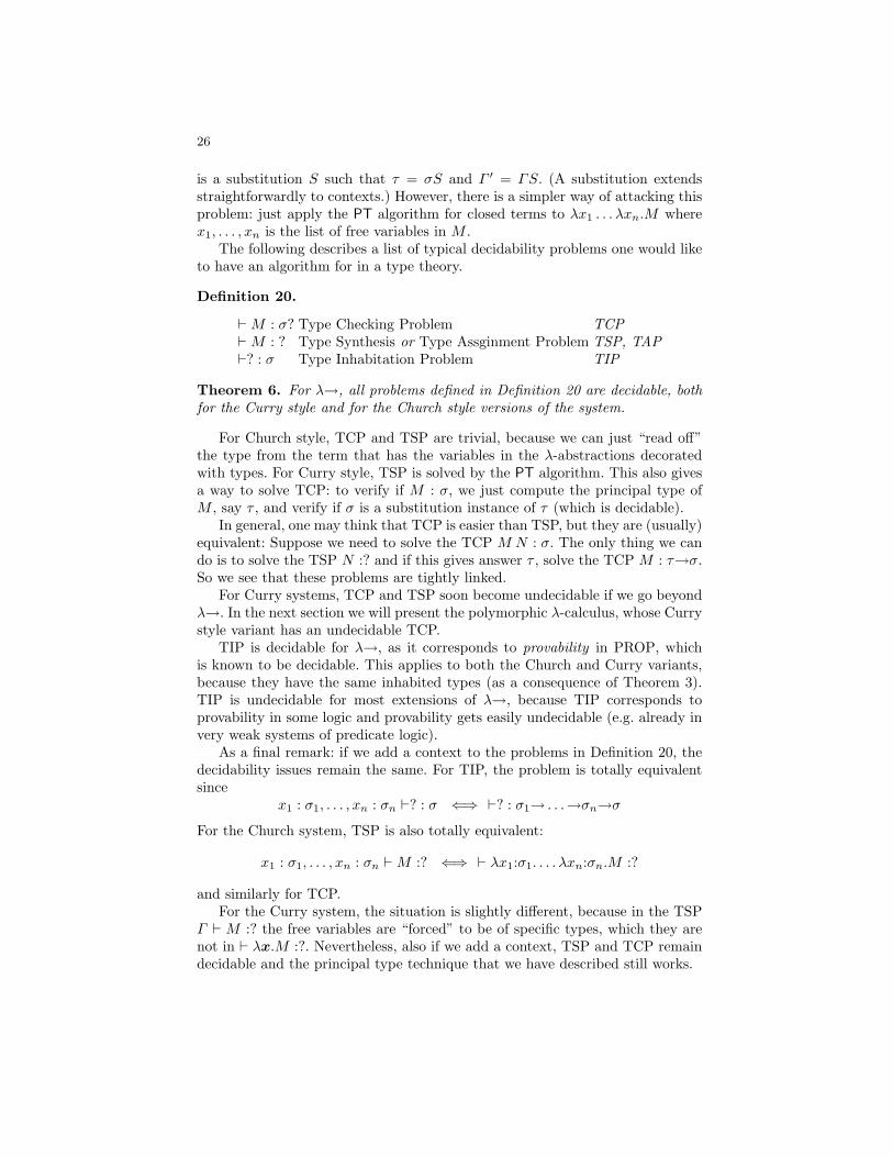
The following describes a list of typical decidability problems one would liketo have an algorithm for in a type theory.

Definition 20.

`M : σ? Type Checking Problem TCP`M : ? Type Synthesis or Type Assginment Problem TSP, TAP`? : σ Type Inhabitation Problem TIP

Theorem 6. For λ→, all problems defined in Definition 20 are decidable, bothfor the Curry style and for the Church style versions of the system.

For Church style, TCP and TSP are trivial, because we can just “read off”the type from the term that has the variables in the λ-abstractions decoratedwith types. For Curry style, TSP is solved by the PT algorithm. This also givesa way to solve TCP: to verify if M : σ, we just compute the principal type ofM , say τ , and verify if σ is a substitution instance of τ (which is decidable).

In general, one may think that TCP is easier than TSP, but they are (usually)equivalent: Suppose we need to solve the TCP M N : σ. The only thing we cando is to solve the TSP N :? and if this gives answer τ , solve the TCP M : τ→σ.So we see that these problems are tightly linked.

For Curry systems, TCP and TSP soon become undecidable if we go beyondλ→. In the next section we will present the polymorphic λ-calculus, whose Currystyle variant has an undecidable TCP.

TIP is decidable for λ→, as it corresponds to provability in PROP, whichis known to be decidable. This applies to both the Church and Curry variants,because they have the same inhabited types (as a consequence of Theorem 3).TIP is undecidable for most extensions of λ→, because TIP corresponds toprovability in some logic and provability gets easily undecidable (e.g. already invery weak systems of predicate logic).

As a final remark: if we add a context to the problems in Definition 20, thedecidability issues remain the same. For TIP, the problem is totally equivalentsince

x1 : σ1, . . . , xn : σn `? : σ ⇐⇒ `? : σ1→ . . .→σn→σ

For the Church system, TSP is also totally equivalent:

x1 : σ1, . . . , xn : σn `M :? ⇐⇒ ` λx1:σ1. . . . λxn:σn.M :?

and similarly for TCP.For the Curry system, the situation is slightly different, because in the TSP

Γ ` M :? the free variables are “forced” to be of specific types, which they arenot in ` λx.M :?. Nevertheless, also if we add a context, TSP and TCP remaindecidable and the principal type technique that we have described still works.

27

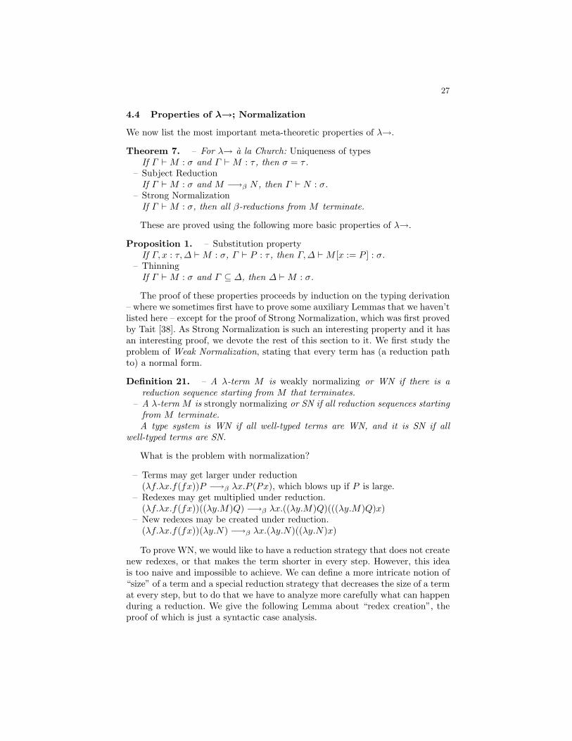
4.4 Properties of λ→; Normalization

We now list the most important meta-theoretic properties of λ→.

Theorem 7. – For λ→ a la Church: Uniqueness of typesIf Γ `M : σ and Γ `M : τ , then σ = τ .

– Subject ReductionIf Γ `M : σ and M −→β N , then Γ ` N : σ.

– Strong NormalizationIf Γ `M : σ, then all β-reductions from M terminate.

These are proved using the following more basic properties of λ→.

Proposition 1. – Substitution propertyIf Γ, x : τ,∆ `M : σ, Γ ` P : τ , then Γ,∆ `M [x := P ] : σ.

– ThinningIf Γ `M : σ and Γ ⊆ ∆, then ∆ `M : σ.

The proof of these properties proceeds by induction on the typing derivation– where we sometimes first have to prove some auxiliary Lemmas that we haven’tlisted here – except for the proof of Strong Normalization, which was first provedby Tait [38]. As Strong Normalization is such an interesting property and it hasan interesting proof, we devote the rest of this section to it. We first study theproblem of Weak Normalization, stating that every term has (a reduction pathto) a normal form.

Definition 21. – A λ-term M is weakly normalizing or WN if there is areduction sequence starting from M that terminates.

– A λ-term M is strongly normalizing or SN if all reduction sequences startingfrom M terminate.A type system is WN if all well-typed terms are WN, and it is SN if all

well-typed terms are SN.

What is the problem with normalization?

– Terms may get larger under reduction(λf.λx.f(fx))P −→β λx.P (Px), which blows up if P is large.

– Redexes may get multiplied under reduction.(λf.λx.f(fx))((λy.M)Q) −→β λx.((λy.M)Q)(((λy.M)Q)x)

– New redexes may be created under reduction.(λf.λx.f(fx))(λy.N) −→β λx.(λy.N)((λy.N)x)

To prove WN, we would like to have a reduction strategy that does not createnew redexes, or that makes the term shorter in every step. However, this ideais too naive and impossible to achieve. We can define a more intricate notion of“size” of a term and a special reduction strategy that decreases the size of a termat every step, but to do that we have to analyze more carefully what can happenduring a reduction. We give the following Lemma about “redex creation”, theproof of which is just a syntactic case analysis.

28

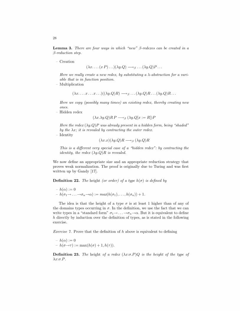
Lemma 3. There are four ways in which “new” β-redexes can be created in aβ-reduction step.

– Creation(λx. . . . (xP ) . . .)(λy.Q) −→β . . . (λy.Q)P . . .

Here we really create a new redex, by substituting a λ-abstraction for a vari-able that is in function position.

– Multiplication

(λx. . . . x . . . x . . .)((λy.Q)R) −→β . . . (λy.Q)R . . . (λy.Q)R . . .

Here we copy (possibly many times) an existing redex, thereby creating newones.

– Hidden redex(λx.λy.Q)RP −→β (λy.Q[x := R])P

Here the redex (λy.Q)P was already present in a hidden form, being “shaded”by the λx; it is revealed by contracting the outer redex.

– Identity(λx.x)(λy.Q)R −→β (λy.Q)R

This is a different very special case of a “hidden redex”: by contracting theidentity, the redex (λy.Q)R is revealed.

We now define an appropriate size and an appropriate reduction strategy thatproves weak normalization. The proof is originally due to Turing and was firstwritten up by Gandy [17].

Definition 22. The height (or order) of a type h(σ) is defined by

– h(α) := 0– h(σ1→ . . .→σn→α) := max(h(σ1), . . . , h(σn)) + 1.

The idea is that the height of a type σ is at least 1 higher than of any ofthe domains types occurring in σ. In the definition, we use the fact that we canwrite types in a “standard form” σ1→ . . .→σn→α. But it is equivalent to defineh directly by induction over the definition of types, as is stated in the followingexercise.

Exercise 7. Prove that the definition of h above is equivalent to defining

– h(α) := 0– h(σ→τ) := max(h(σ) + 1, h(τ)).

Definition 23. The height of a redex (λx:σ.P )Q is the height of the type ofλx:σ.P .

29

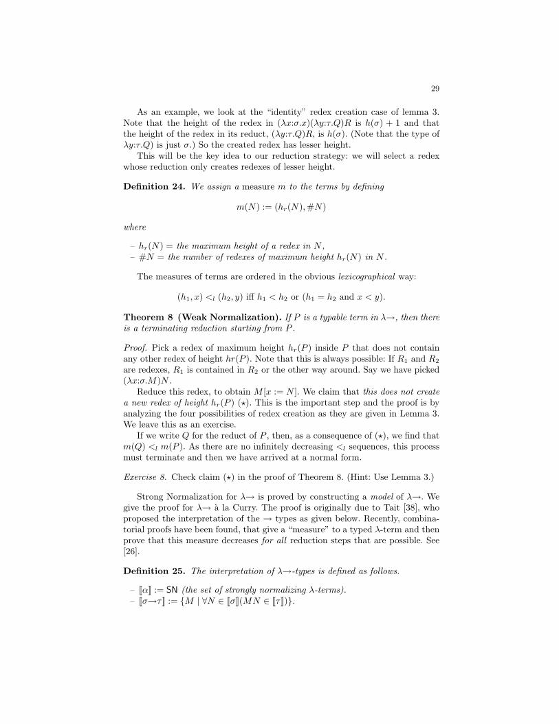
As an example, we look at the “identity” redex creation case of lemma 3.Note that the height of the redex in (λx:σ.x)(λy:τ.Q)R is h(σ) + 1 and thatthe height of the redex in its reduct, (λy:τ.Q)R, is h(σ). (Note that the type ofλy:τ.Q) is just σ.) So the created redex has lesser height.

This will be the key idea to our reduction strategy: we will select a redexwhose reduction only creates redexes of lesser height.

Definition 24. We assign a measure m to the terms by defining

m(N) := (hr(N),#N)

where

– hr(N) = the maximum height of a redex in N ,– #N = the number of redexes of maximum height hr(N) in N .

The measures of terms are ordered in the obvious lexicographical way:

(h1, x) <l (h2, y) iff h1 < h2 or (h1 = h2 and x < y).

Theorem 8 (Weak Normalization). If P is a typable term in λ→, then thereis a terminating reduction starting from P .

Proof. Pick a redex of maximum height hr(P ) inside P that does not containany other redex of height hr(P ). Note that this is always possible: If R1 and R2

are redexes, R1 is contained in R2 or the other way around. Say we have picked(λx:σ.M)N .

Reduce this redex, to obtain M [x := N ]. We claim that this does not createa new redex of height hr(P ) (?). This is the important step and the proof is byanalyzing the four possibilities of redex creation as they are given in Lemma 3.We leave this as an exercise.

If we write Q for the reduct of P , then, as a consequence of (?), we find thatm(Q) <l m(P ). As there are no infinitely decreasing <l sequences, this processmust terminate and then we have arrived at a normal form.

Exercise 8. Check claim (?) in the proof of Theorem 8. (Hint: Use Lemma 3.)

Strong Normalization for λ→ is proved by constructing a model of λ→. Wegive the proof for λ→ a la Curry. The proof is originally due to Tait [38], whoproposed the interpretation of the → types as given below. Recently, combina-torial proofs have been found, that give a “measure” to a typed λ-term and thenprove that this measure decreases for all reduction steps that are possible. See[26].

Definition 25. The interpretation of λ→-types is defined as follows.

– [[α]] := SN (the set of strongly normalizing λ-terms).– [[σ→τ ]] := M | ∀N ∈ [[σ]](MN ∈ [[τ ]]).

30

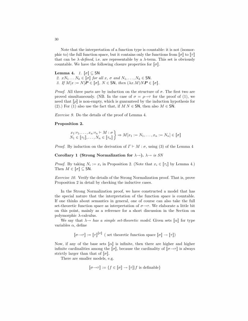
Note that the interpretation of a function type is countable: it is not (isomor-phic to) the full function space, but it contains only the functions from [[σ]] to [[τ ]]that can be λ-defined, i.e. are representable by a λ-term. This set is obviouslycountable. We have the following closure properties for [[σ]].

Lemma 4. 1. [[σ]] ⊆ SN2. xN1 . . . Nk ∈ [[σ]] for all x, σ and N1, . . . , Nk ∈ SN.3. If M [x := N ]P ∈ [[σ]], N ∈ SN, then (λx.M)NP ∈ [[σ]].

Proof. All three parts are by induction on the structure of σ. The first two areproved simultaneously. (NB. In the case of σ = ρ→τ for the proof of (1), weneed that [[ρ]] is non-empty, which is guaranteed by the induction hypothesis for(2).) For (1) also use the fact that, if M N ∈ SN, then also M ∈ SN.

Exercise 9. Do the details of the proof of Lemma 4.

Proposition 2.

x1:τ1, . . . , xn:τn `M : σN1 ∈ [[τ1]], . . . , Nn ∈ [[τn]]

⇒M [x1 := N1, . . . , xn := Nn] ∈ [[σ]]

Proof. By induction on the derivation of Γ `M : σ, using (3) of the Lemma 4

Corollary 1 (Strong Normalization for λ→). λ→ is SN

Proof. By taking Ni := xi in Proposition 2. (Note that xi ∈ [[τi]] by Lemma 4.)Then M ∈ [[σ]] ⊆ SN.

Exercise 10. Verify the details of the Strong Normalization proof. That is, proveProposition 2 in detail by checking the inductive cases.

In the Strong Normalization proof, we have constructed a model that hasthe special nature that the interpretation of the function space is countable.If one thinks about semantics in general, one of course can also take the fullset-theoretic function space as interpretation of σ→τ . We elaborate a little biton this point, mainly as a reference for a short discussion in the Section onpolymorphic λ-calculus.

We say that λ→ has a simple set-theoretic model. Given sets [[α]] for typevariables α, define

[[σ→τ ]] := [[τ ]][[σ]] ( set theoretic function space [[σ]]→ [[τ ]])

Now, if any of the base sets [[α]] is infinite, then there are higher and higherinfinite cardinalities among the [[σ]], because the cardinality of [[σ→τ ]] is alwaysstrictly larger than that of [[σ]].

There are smaller models, e.g.

[[σ→τ ]] := f ∈ [[σ]]→ [[τ ]]|f is definable

31

where definability means that it can be constructed in some formal system. Thisrestricts the collection to a countable set. As an example we have seen in the SNproof the following interpretation

[[σ→τ ]] := f ∈ [[σ]]→ [[τ ]]|f is λ-definable

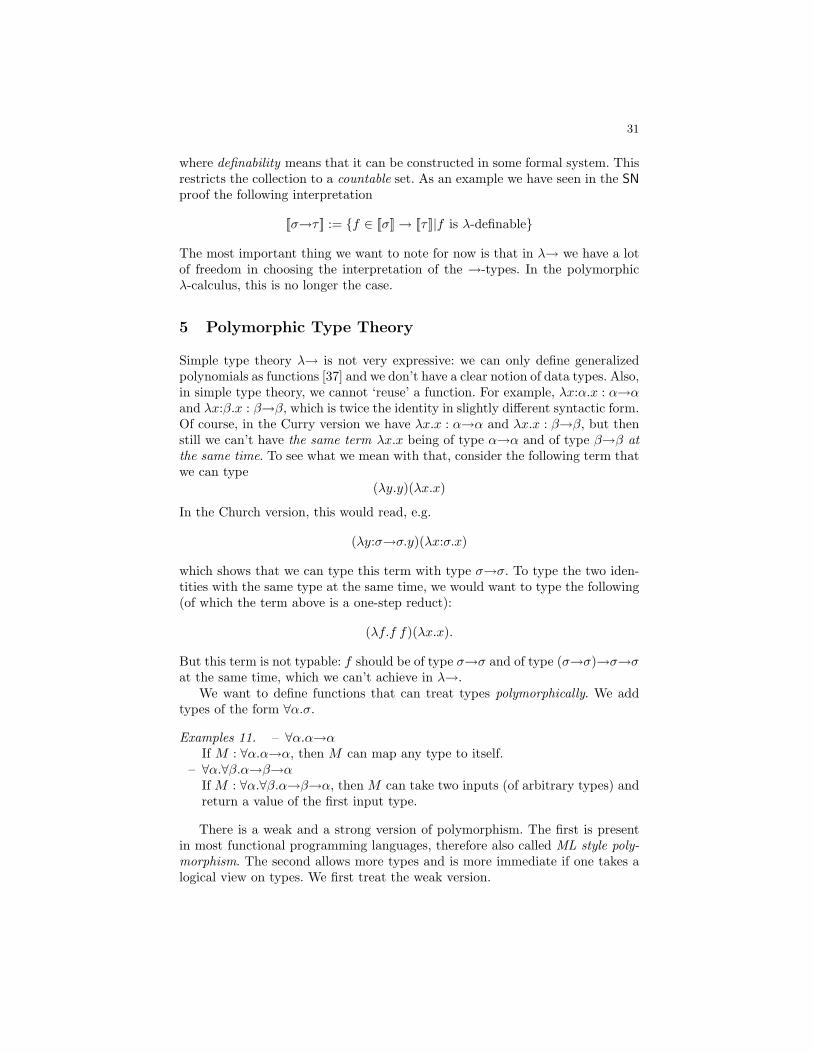
The most important thing we want to note for now is that in λ→ we have a lotof freedom in choosing the interpretation of the →-types. In the polymorphicλ-calculus, this is no longer the case.

5 Polymorphic Type Theory

Simple type theory λ→ is not very expressive: we can only define generalizedpolynomials as functions [37] and we don’t have a clear notion of data types. Also,in simple type theory, we cannot ‘reuse’ a function. For example, λx:α.x : α→αand λx:β.x : β→β, which is twice the identity in slightly different syntactic form.Of course, in the Curry version we have λx.x : α→α and λx.x : β→β, but thenstill we can’t have the same term λx.x being of type α→α and of type β→β atthe same time. To see what we mean with that, consider the following term thatwe can type

(λy.y)(λx.x)

In the Church version, this would read, e.g.

(λy:σ→σ.y)(λx:σ.x)

which shows that we can type this term with type σ→σ. To type the two iden-tities with the same type at the same time, we would want to type the following(of which the term above is a one-step reduct):

(λf.f f)(λx.x).

But this term is not typable: f should be of type σ→σ and of type (σ→σ)→σ→σat the same time, which we can’t achieve in λ→.

We want to define functions that can treat types polymorphically. We addtypes of the form ∀α.σ.

Examples 11. – ∀α.α→αIf M : ∀α.α→α, then M can map any type to itself.

– ∀α.∀β.α→β→αIf M : ∀α.∀β.α→β→α, then M can take two inputs (of arbitrary types) andreturn a value of the first input type.

There is a weak and a strong version of polymorphism. The first is presentin most functional programming languages, therefore also called ML style poly-morphism. The second allows more types and is more immediate if one takes alogical view on types. We first treat the weak version.

32

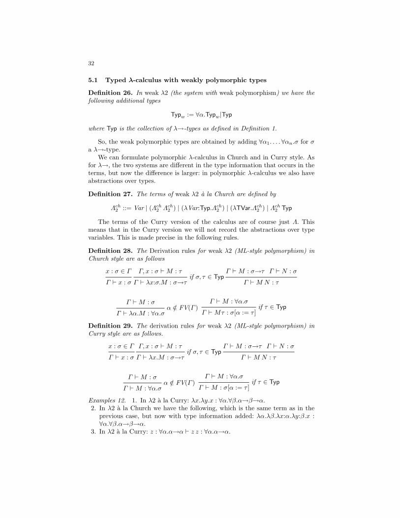
5.1 Typed λ-calculus with weakly polymorphic types

Definition 26. In weak λ2 (the system with weak polymorphism) we have thefollowing additional types

Typw := ∀α.Typw|Typ

where Typ is the collection of λ→-types as defined in Definition 1.

So, the weak polymorphic types are obtained by adding ∀α1. . . .∀αn.σ for σa λ→-type.

We can formulate polymorphic λ-calculus in Church and in Curry style. Asfor λ→, the two systems are different in the type information that occurs in theterms, but now the difference is larger: in polymorphic λ-calculus we also haveabstractions over types.

Definition 27. The terms of weak λ2 a la Church are defined by

Λch2 ::= Var | (Λch2 Λch2 ) | (λVar:Typ.Λch2 ) | (λTVar.Λch2 ) | Λch2 Typ

The terms of the Curry version of the calculus are of course just Λ. Thismeans that in the Curry version we will not record the abstractions over typevariables. This is made precise in the following rules.

Definition 28. The Derivation rules for weak λ2 (ML-style polymorphism) inChurch style are as follows

x : σ ∈ Γ

Γ ` x : σ

Γ, x : σ `M : τif σ, τ ∈ Typ

Γ ` λx:σ.M : σ→τ

Γ `M : σ→τ Γ ` N : σ

Γ `M N : τ

Γ `M : σα /∈ FV(Γ )

Γ ` λα.M : ∀α.σ

Γ `M : ∀α.σif τ ∈ Typ

Γ `Mτ : σ[α := τ ]

Definition 29. The derivation rules for weak λ2 (ML-style polymorphism) inCurry style are as follows.

x : σ ∈ Γ

Γ ` x : σ

Γ, x : σ `M : τif σ, τ ∈ Typ

Γ ` λx.M : σ→τ

Γ `M : σ→τ Γ ` N : σ

Γ `M N : τ

Γ `M : σα /∈ FV(Γ )

Γ `M : ∀α.σ

Γ `M : ∀α.σif τ ∈ Typ

Γ `M : σ[α := τ ]

Examples 12. 1. In λ2 a la Curry: λx.λy.x : ∀α.∀β.α→β→α.2. In λ2 a la Church we have the following, which is the same term as in the

previous case, but now with type information added: λα.λβ.λx:α.λy:β.x :∀α.∀β.α→β→α.

3. In λ2 a la Curry: z : ∀α.α→α ` z z : ∀α.α→α.

33

4. In λ2 a la Church, we can annotate this term with type information to obtain:z : ∀α.α→α ` λα.z (α→α) (z α) : ∀α.α→α.

5. We do not have ` λz.z z : . . .

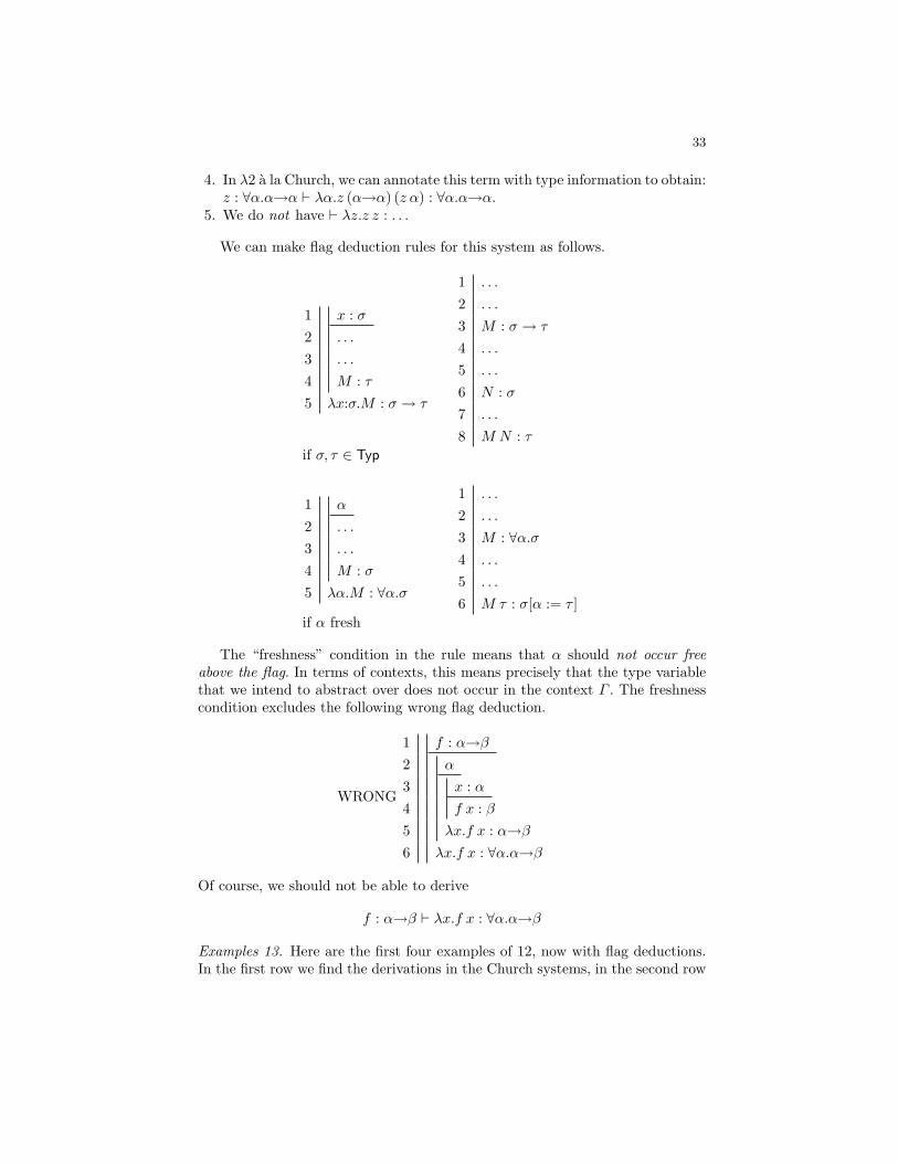
We can make flag deduction rules for this system as follows.

1 x : σ2 . . .

3 . . .

4 M : τ5 λx:σ.M : σ → τ

1 . . .

2 . . .

3 M : σ → τ

4 . . .

5 . . .

6 N : σ7 . . .

8 M N : τif σ, τ ∈ Typ

1 α

2 . . .

3 . . .

4 M : σ5 λα.M : ∀α.σ

1 . . .

2 . . .

3 M : ∀α.σ4 . . .

5 . . .

6 M τ : σ[α := τ ]if α fresh

The “freshness” condition in the rule means that α should not occur freeabove the flag. In terms of contexts, this means precisely that the type variablethat we intend to abstract over does not occur in the context Γ . The freshnesscondition excludes the following wrong flag deduction.

WRONG

1 f : α→β2 α

3 x : α4 f x : β5 λx.f x : α→β6 λx.f x : ∀α.α→β

Of course, we should not be able to derive

f : α→β ` λx.f x : ∀α.α→β

Examples 13. Here are the first four examples of 12, now with flag deductions.In the first row we find the derivations in the Church systems, in the second row

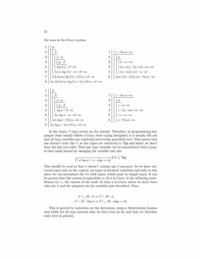
34

the ones in the Curry system.

1 α

2 β

3 x : α4 y : β5 λy:β.x : β→α6 λx:α.λy:β.x : α→β→α7 λβ.λx:α.λy:β.x : ∀β.α→β→α8 λα.λβ.λx:α.λy:β.x : ∀α.∀β.α→β→α

1 z : ∀α.α→α2 α

3 z α : α→α4 z (α→α) : (α→α)→α→α5 z (α→α)(z α) : α→α6 λα.z (α→α)(z α) : ∀α.α→α

1 α

2 β

3 x : α4 y : β5 λy.x : β→α6 λx.λy.x : α→β→α7 λx.λy.x : ∀β.α→β→α8 λx.λy.x : ∀α.∀β.α→β→α

1 z : ∀α.α→α2 α

3 z : α→α4 z : (α→α)→α→α5 z z : α→α6 z z : ∀α.α→α

In the types, ∀ only occurs on the outside. Therefore, in programming lan-guages (that usually follow a Curry style typing discipline) it is usually left outand all type variables are implicitly universally quantified over. This means thatone doesn’t write the ∀, so the types are restricted to Typ and hence we don’thave the last two rules. That any type variable can be instantiated with a type,is then made formal by changing the variable rule into

if τ ⊆ TypΓ, x:∀α.σ ` x : σ[α := τ ]

This should be read as that σ doesn’t contain any ∀ anymore. So we have uni-versal types only in the context (as types of declared variables) and only at thisplace we can instantiate the ∀α with types, which must be simple types. It canbe proven that this system is equivalent to λ2 a la Curry in the following sense.Denote by `v the variant of the weak λ2 rules a la Curry where we don’t haverules for ∀ and the adapted rule for variables just described. Then

Γ `v M : σ ⇒ Γ `M : σΓ `M : ∀α.σ ⇒ Γ `v M : σ[α := τ ]

This is proved by induction on the derivation, using a Substitution Lemmathat holds for all type systems that we have seen so far and that we thereforestate here in general.

35

Lemma 5 (Substitution for types). If Γ ` M : σ, then Γ [α := τ ] ` M :σ[α := τ ], for all systems a la Curry defined so far.For the Church systems we have types in the terms. Then the Substitution Lemmastates: If Γ `M : σ, then Γ [α := τ ] `M [α := τ ] : σ[α := τ ].

For all systems, this Lemma is proved by a straightforward induction overthe derivation.

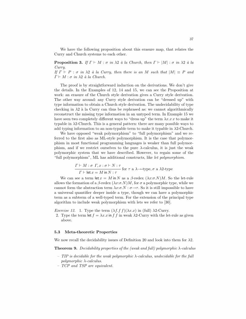
With weak polymorphism, type checking is still decidable: the principal typesalgorithm can be extended to incorporate type schemes: types of the form ∀α.σ.We have observed that weak polymorphism allows terms to have many (poly-morphic) types, but we cannot abstract over variables of these types. This isallowed with full polymorphism, also called system F style polymorphism.

5.2 Typed λ-calculus with full polymorphism

Definition 30. The types of λ2 with full (system F-style) polymorphism are

Typ2 := TVar | (Typ2→Typ2) | ∀α.Typ2

1. The derivation rules for λ2 with full (system F-style) polymorphism in Currystyle are as follows. (Note that σ and τ range over Typ2.)

x : σ ∈ Γ

Γ ` x : σ

Γ, x : σ `M : τ

Γ ` λx.M : σ→τ

Γ `M : σ→τ Γ ` N : σ

Γ `M N : τ

Γ `M : σα /∈ FV(Γ )

Γ `M : ∀α.σ

Γ `M : ∀α.σ

Γ `M : σ[α := τ ]

2. The derivation rules for λ2 with full (system F-style) polymorphism inChurch style are as follows. (Again, note that σ and τ range over Typ2.)

x : σ ∈ Γ

Γ ` x : σ

Γ, x : σ `M : τ

Γ ` λx:σ.M : σ→τ

Γ `M : σ→τ Γ ` N : σ

Γ `M N : τ

Γ `M : σα /∈ FV(Γ )

Γ ` λα.M : ∀α.σ

Γ `M : ∀α.σ

Γ `Mτ : σ[α := τ ]

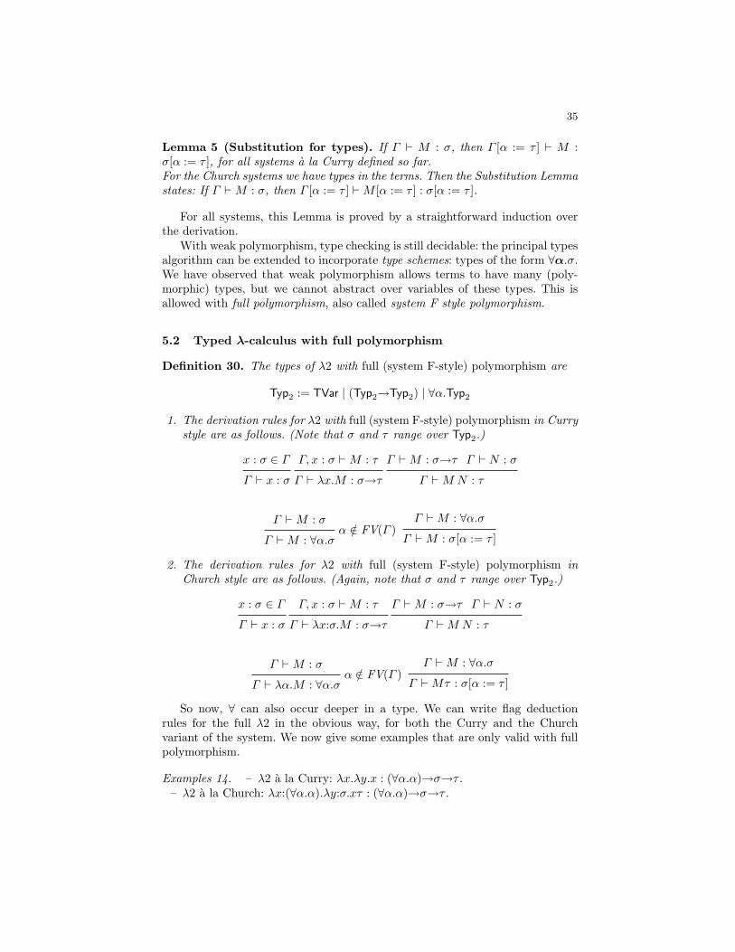
So now, ∀ can also occur deeper in a type. We can write flag deductionrules for the full λ2 in the obvious way, for both the Curry and the Churchvariant of the system. We now give some examples that are only valid with fullpolymorphism.

Examples 14. – λ2 a la Curry: λx.λy.x : (∀α.α)→σ→τ .– λ2 a la Church: λx:(∀α.α).λy:σ.xτ : (∀α.α)→σ→τ .

36

Here are the flag deductions that prove the two typings in the Examples.

1 x : ∀α.α2 y : σ3 x τ : τ4 λy:σ.x τ : σ→τ5 λx:∀α.α.λy:σ.x τ : (∀α.α)→σ→τ

1 x : ∀α.α2 y : σ3 x : τ4 λy.x : σ→τ5 λx.λy.x : (∀α.α)→σ→τ

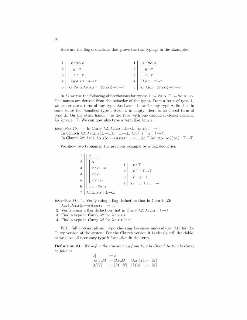
In λ2 we use the following abbreviations for types: ⊥ := ∀α.α, > := ∀α.α→α.The names are derived from the behavior of the types. From a term of type ⊥,we can create a term of any type: λx:⊥.xσ : ⊥→σ for any type σ. So ⊥ is insome sense the “smallest type”. Also, ⊥ is empty: there is no closed term oftype ⊥. On the other hand, > is the type with one canonical closed element:λα.λx:α.x : >. We can now also type a term like λx.x x.

Examples 15. – In Curry λ2: λx.xx : ⊥→⊥, λx.xx : >→>– In Church λ2: λx:⊥.x(⊥→⊥)x : ⊥→⊥, λx:>.x>x : >→>.– In Church λ2: λx:⊥.λα.x(α→α)(xα) : ⊥→⊥, λx:>.λα.x(α→α)(xα) : >→>.

We show two typings in the previous example by a flag deduction.

1 x : ⊥2 α

3 x : α→α4 x : α5 xx : α6 xx : ∀α.α7 λx:⊥.x x : ⊥→⊥

1 x : >2 x> : >→>3 x>x : >4 λx:>.x>x : >→>

Exercises 11. 1. Verify using a flag deduction that in Church λ2:λx:>.λα.x(α→α)(xα) : >→>.

2. Verify using a flag deduction that in Curry λ2: λx.xx : >→>3. Find a type in Curry λ2 for λx.x xx4. Find a type in Curry λ2 for λx.x x (xx)

With full polymorphism, type checking becomes undecidable [41] for theCurry version of the system. For the Church version it is clearly still decidable,as we have all necessary type information in the term.

Definition 31. We define the erasure map from λ2 a la Church to λ2 a la Curryas follows.

|x| := x|λx:σ.M | := |λx.M | |λα.M | := |M ||MN | := |M | |N | |Mσ| := |M |

37

We have the following proposition about this erasure map, that relates theCurry and Church systems to each other.

Proposition 3. If Γ ` M : σ in λ2 a la Church, then Γ ` |M | : σ in λ2 a laCurry.If Γ ` P : σ in λ2 a la Curry, then there is an M such that |M | ≡ P andΓ `M : σ in λ2 a la Church.

The proof is by straightforward induction on the derivations. We don’t givethe details. In the Examples of 12, 14 and 15, we can see the Proposition atwork: an erasure of the Church style derivation gives a Curry style derivation.The other way around: any Curry style derivation can be “dressed up” withtype information to obtain a Church style derivation. The undecidability of typechecking in λ2 a la Curry can thus be rephrased as: we cannot algorithmicallyreconstruct the missing type information in an untyped term. In Example 15 wehave seen two completely different ways to “dress up” the term λx.x x to make ittypable in λ2-Church. This is a general pattern: there are many possible ways toadd typing information to an non-typable term to make it typable in λ2-Church.

We have opposed “weak polymorphism” to “full polymorphism” and we re-ferred to the first also as ML-style polymorphism. It is the case that polymor-phism in most functional programming languages is weaker than full polymor-phism, and if we restrict ourselves to the pure λ-calculus, it is just the weakpolymorphic system that we have described. However, to regain some of the“full polymorphism”, ML has additional constructs, like let polymorphism.

Γ `M : σ Γ, x : σ ` N : τfor τ a λ→-type, σ a λ2-type

Γ ` letx = M inN : τWe can see a term letx = M inN as a β-redex (λx:σ.N)M . So the let-rule

allows the formation of a β-redex (λx:σ.N)M , for σ a polymorphic type, while wecannot form the abstraction term λx:σ.N : σ→τ . So it is still impossible to havea universal quantifier deeper inside a type, though we can have a polymorphicterm as a subterm of a well-typed term. For the extension of the principal typealgorithm to include weak polymorphism with lets we refer to [30].

Exercise 12. 1. Type the term (λf.f f)(λx.x) in (full) λ2-Curry.2. Type the term let f = λx.x in f f in weak λ2-Curry with the let-rule as given

above.

5.3 Meta-theoretic Properties

We now recall the decidability issues of Definition 20 and look into them for λ2.

Theorem 9. Decidability properties of the (weak and full) polymorphic λ-calculus

– TIP is decidable for the weak polymorphic λ-calculus, undecidable for the fullpolymorphic λ-calculus.

– TCP and TSP are equivalent.

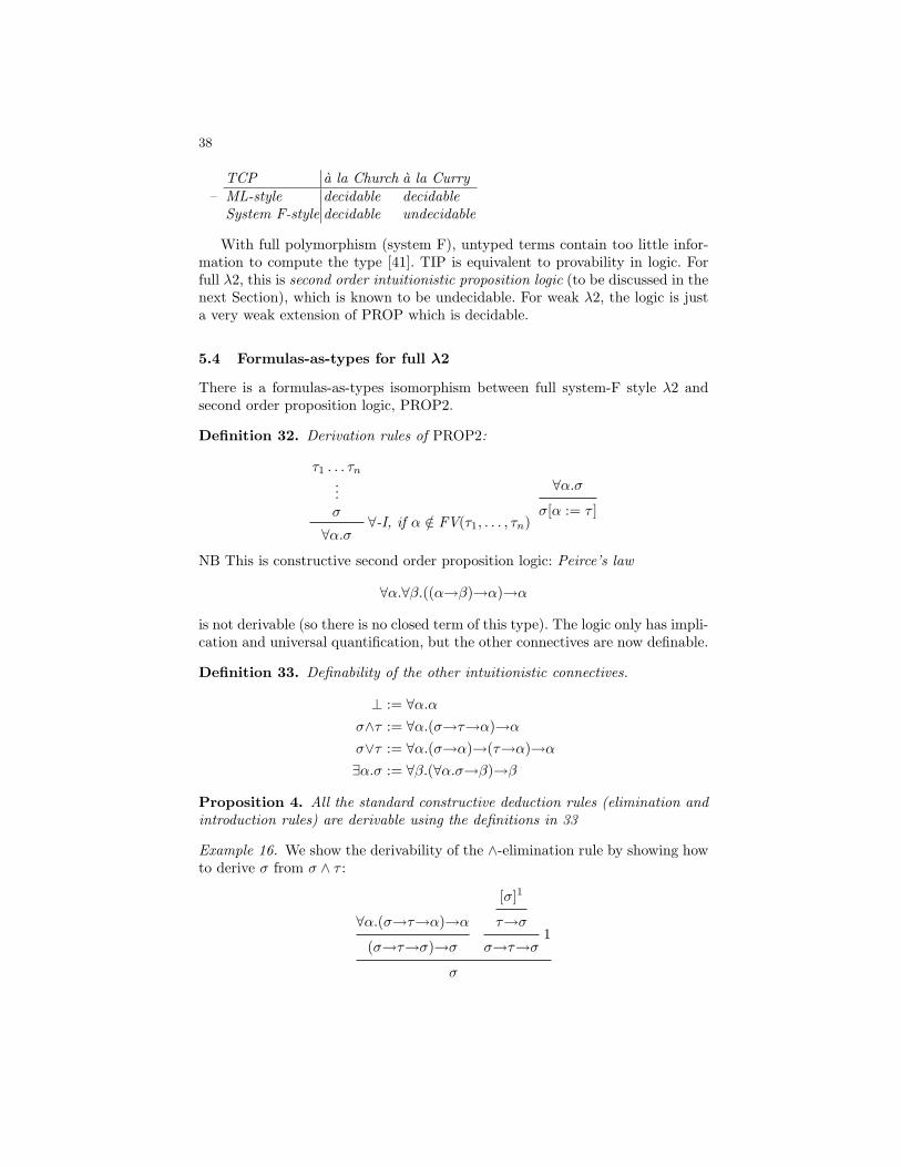
38

–TCP a la Church a la CurryML-style decidable decidableSystem F-style decidable undecidable

With full polymorphism (system F), untyped terms contain too little infor-mation to compute the type [41]. TIP is equivalent to provability in logic. Forfull λ2, this is second order intuitionistic proposition logic (to be discussed in thenext Section), which is known to be undecidable. For weak λ2, the logic is justa very weak extension of PROP which is decidable.

5.4 Formulas-as-types for full λ2

There is a formulas-as-types isomorphism between full system-F style λ2 andsecond order proposition logic, PROP2.

Definition 32. Derivation rules of PROP2:

τ1 . . . τn...σ

∀-I, if α /∈ FV(τ1, . . . , τn)∀α.σ

∀α.σ

σ[α := τ ]

NB This is constructive second order proposition logic: Peirce’s law

∀α.∀β.((α→β)→α)→α

is not derivable (so there is no closed term of this type). The logic only has impli-cation and universal quantification, but the other connectives are now definable.

Definition 33. Definability of the other intuitionistic connectives.

⊥ := ∀α.ασ∧τ := ∀α.(σ→τ→α)→ασ∨τ := ∀α.(σ→α)→(τ→α)→α∃α.σ := ∀β.(∀α.σ→β)→β

Proposition 4. All the standard constructive deduction rules (elimination andintroduction rules) are derivable using the definitions in 33

Example 16. We show the derivability of the ∧-elimination rule by showing howto derive σ from σ ∧ τ :

∀α.(σ→τ→α)→α

(σ→τ→σ)→σ

[σ]1

τ→σ1

σ→τ→σ

σ

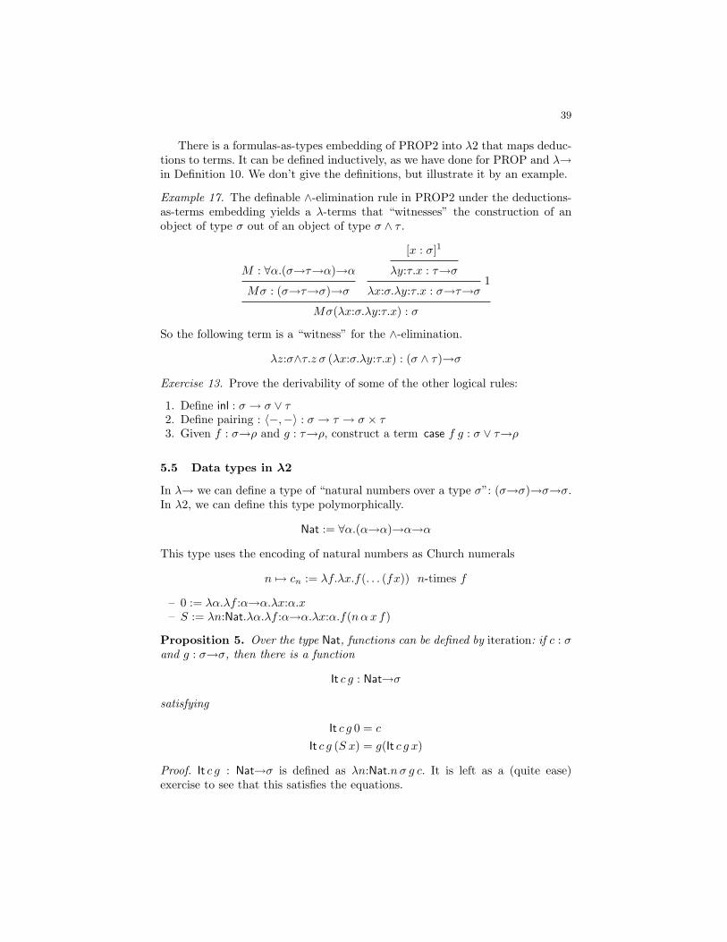
39

There is a formulas-as-types embedding of PROP2 into λ2 that maps deduc-tions to terms. It can be defined inductively, as we have done for PROP and λ→in Definition 10. We don’t give the definitions, but illustrate it by an example.

Example 17. The definable ∧-elimination rule in PROP2 under the deductions-as-terms embedding yields a λ-terms that “witnesses” the construction of anobject of type σ out of an object of type σ ∧ τ .

M : ∀α.(σ→τ→α)→α

Mσ : (σ→τ→σ)→σ

[x : σ]1

λy:τ.x : τ→σ1

λx:σ.λy:τ.x : σ→τ→σ

Mσ(λx:σ.λy:τ.x) : σ

So the following term is a “witness” for the ∧-elimination.

λz:σ∧τ.z σ (λx:σ.λy:τ.x) : (σ ∧ τ)→σ

Exercise 13. Prove the derivability of some of the other logical rules:

1. Define inl : σ → σ ∨ τ2. Define pairing : 〈−,−〉 : σ → τ → σ × τ3. Given f : σ→ρ and g : τ→ρ, construct a term case f g : σ ∨ τ→ρ

5.5 Data types in λ2

In λ→ we can define a type of “natural numbers over a type σ”: (σ→σ)→σ→σ.In λ2, we can define this type polymorphically.

Nat := ∀α.(α→α)→α→α

This type uses the encoding of natural numbers as Church numerals

n 7→ cn := λf.λx.f(. . . (fx)) n-times f

– 0 := λα.λf :α→α.λx:α.x– S := λn:Nat.λα.λf :α→α.λx:α.f(nαx f)

Proposition 5. Over the type Nat, functions can be defined by iteration: if c : σand g : σ→σ, then there is a function

It c g : Nat→σ

satisfying

It c g 0 = c

It c g (S x) = g(It c g x)

Proof. It c g : Nat→σ is defined as λn:Nat.n σ g c. It is left as a (quite ease)exercise to see that this satisfies the equations.

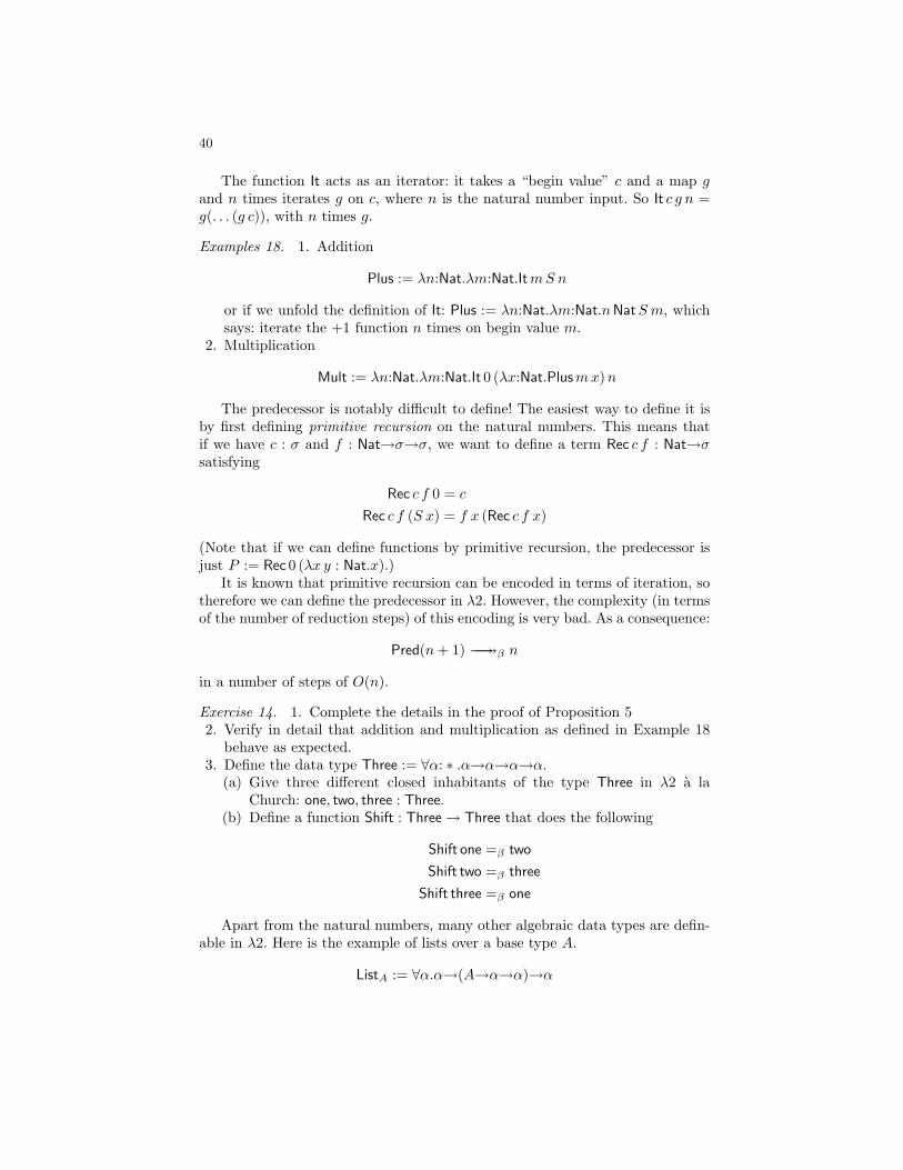
40

The function It acts as an iterator: it takes a “begin value” c and a map gand n times iterates g on c, where n is the natural number input. So It c g n =g(. . . (g c)), with n times g.

Examples 18. 1. Addition

Plus := λn:Nat.λm:Nat.ItmS n

or if we unfold the definition of It: Plus := λn:Nat.λm:Nat.nNatS m, whichsays: iterate the +1 function n times on begin value m.

2. Multiplication

Mult := λn:Nat.λm:Nat.It 0 (λx:Nat.Plusmx)n

The predecessor is notably difficult to define! The easiest way to define it isby first defining primitive recursion on the natural numbers. This means thatif we have c : σ and f : Nat→σ→σ, we want to define a term Rec c f : Nat→σsatisfying

Rec c f 0 = c

Rec c f (S x) = f x (Rec c f x)

(Note that if we can define functions by primitive recursion, the predecessor isjust P := Rec 0 (λx y : Nat.x).)

It is known that primitive recursion can be encoded in terms of iteration, sotherefore we can define the predecessor in λ2. However, the complexity (in termsof the number of reduction steps) of this encoding is very bad. As a consequence:

Pred(n+ 1) −→−→β n

in a number of steps of O(n).

Exercise 14. 1. Complete the details in the proof of Proposition 52. Verify in detail that addition and multiplication as defined in Example 18

behave as expected.3. Define the data type Three := ∀α: ∗ .α→α→α→α.

(a) Give three different closed inhabitants of the type Three in λ2 a laChurch: one, two, three : Three.

(b) Define a function Shift : Three→ Three that does the following

Shift one =β two

Shift two =β three

Shift three =β one

Apart from the natural numbers, many other algebraic data types are defin-able in λ2. Here is the example of lists over a base type A.

ListA := ∀α.α→(A→α→α)→α

41

The representation of lists over A as terms of this type uses the followingencoding

[a1, a2, . . . , an] 7→ λx.λf.fa1(fa2(. . . (fanx))) n-times f

We can now define the constructors Nil (empty list) and Cons (to “cons” anelement to a list) as follows.

– Nil := λα.λx:α.λf :A→α→α.x– Cons := λa:A.λl:ListA.λα.λx:α.λf :A→α→α.f a(l α x f)

Note that the definition of Cons conforms with the representation of lists givenabove.

Proposition 6. Over the type ListA we can define functions by iteration: if c : σand g : A→σ→σ, then there is a function

It c g : ListA→σ

satisfying

It c gNil = c

It c g (Cons a l) = g a (It c g l)

Proof. It c g : ListA→σ is defined as λl:ListA.l σ c g. This satisfies the equations inthe proposition. Basically, we have, for l = [a1, . . . , an], It c g l = g a1(. . . (g an c))(n times g).

Example 19. A standard function one wants to define over lists is the “map”function, which given a function on the carrier type, extends it to a function onthe lists over this carrier type. Given f : σ→τ , Map f : Listσ→Listτ should applyf to all elements in a list. It is defined by

Map := λf :σ→τ.It Nil(λx:σ.λl:Listτ .Cons(f x)l).

Then

Map f Nil = Nil

Map f (Cons a k) = It Nil(λx:σ.λl:Listτ .Cons(f x)l) (Cons a k)= (λx:σ.λl:Listτ .Cons(f x)l)a(Map f k)= Cons(f a)(Map f k)

This is exactly the recursion equation for Map that we would expect.

Many more data-types can be defined in λ2. The product of two data-types isdefined in the same way as the (logical) conjunction: σ×τ := ∀α.(σ→τ→α)→α.we have already seen how to define projections and pairing (the ∧-elimination

42

and ∧-introduction rules). The disjoint union (or sum) of two data-types is de-fined in the same way as the logical disjunction: σ+τ := ∀α.(σ→α)→(τ→α)→α.We can define inl, inr and case . The type of binary trees with nodes in A andleaves in B can be defined as follows.

TreeA,B := ∀α.(B→α)→(A→α→α→α)→α

and we define leaf : B→TreeA,B by leaf := λb:B.λα.λl:B→α.λj:A→α→α→α.l b.

Exercises 15. – Define a function of type ListA→Nat that computes the lengthof a list.

– Define join : TreeA,B → TreeA,B → A → TreeA,B that takes two trees and anode label and builds a tree.

– Define a function TreeSum : TreeNat,Nat→Nat that computes the sum of allleaves and nodes in a binary tree.

– Give the iteration scheme over binary trees and show that it is definable inλ2.

5.6 Meta-theory of λ2; Strong Normalization

Theorem 10. – For λ2 a la Church: Uniqueness of typesIf Γ `M : σ and Γ `M : τ , then σ = τ .

– Subject ReductionIf Γ `M : σ and M −→βη N , then Γ ` N : σ.

– Strong NormalizationIf Γ `M : σ, then all β-reductions from M terminate.

The third property is remarkably complicated and we address it in detailbelow. The first two are proved by induction on the derivation, using some othermeta-theoretic properties, that one also proves by induction over the derivation(the Substitution Property we have already seen for types; this is the sameproperty for terms):

Proposition 7. – Substitution propertyIf Γ, x : τ,∆ `M : σ, Γ ` P : τ , then Γ,∆ `M [x := P ] : σ.

– ThinningIf Γ `M : σ and Γ ⊆ ∆, then ∆ `M : σ.

We now elaborate on the proof of Strong Normalization of β-reduction forλ2. The proof is an extension of the Tait proof of SN for λ→, but it needs somecrucial extra ingredients that have been developed by Girard [21]. We motivatethese additional notions below.

In λ2 a la Church there are two kinds of β-reductions:

– Kind 1, term-applied-to-term: (λx:σ.M)P −→β M [x := P ]– Kind 2, term-applied-to-type: (λα.M)τ −→β M [α := τ ]

43

The second kind of reductions does no harm: (i) there are no infinite β-reduction paths with solely reductions of kind 2; (ii) if M −→β N with a re-duction of kind 2, then |M | ≡ |N |. So, if there is an infinite β-reduction inλ2-Church, then there is one in λ2-Curry and we are done if we prove SN for λ2a la Curry.

Recall the model construction in the proof for λ→:

– [[α]] := SN.– [[σ→τ ]] := M | ∀N ∈ [[σ]](MN ∈ [[τ ]]).

So, now the question is: How to define [[∀α.σ]]? A natural guess would beto define [[∀α.σ]] := ΠX∈U [[σ]]α:=X , where U is some set capturing all possibleinterpretations of types. This Π-set is a set of functions that take an element Xof U (an interpretation of a type) and yield an element of the interpretation ofσ where we assign X to α.

But now the problem is that ΠX∈U [[σ]]α:=X gets too big: if there is any typewith more than one element (something we would require for a model), thencard(ΠX∈U [[σ]]α:=X) > card(U). The cardinality of the interpretation of ∀α.σwould be larger than the set it is a member of and that’s impossible. So wecannot interpret the ∀ as a Π-set (or a union for the same reason).

Girard has given the solution to this problem: [[∀α.σ]] should be very small:

[[∀α.σ]] :=⋂X∈U

[[σ]]α:=X

This conforms with the idea that ∀α.σ is the type of terms that act parametricallyon a type. A lot of literature has been devoted to the nature of polymorphism,for which the terminology parametricity has been introduced, intuitively sayingthat a function operates on types without looking into them. So a parametricfunction cannot act differently on Nat and Bool. This implies, e.g. that thereis only one parametric function from α to α: the identity. See [1] for more onparametricity.

The second important novelty of Girard is the actual definition of U , thecollection of all possible interpretations of types. U will be defined as SAT, thecollection of saturated sets of (untyped) λ-terms.

Definition 34. X ⊂ Λ is saturated if

– xP1 . . . Pn ∈ X (for all x ∈ Var, P1, . . . , Pn ∈ SN)– X ⊆ SN– If M [x := N ]P ∈ X and N ∈ SN, then (λx.M)NP ∈ X.

The definition of saturated sets basically arises by taking the closure prop-erties that we proved for the interpretation of λ→-types as a definition of thecollection of possible interpretation of λ2-types.

Definition 35. Let ρ : TVar → SAT be a valuation of type variables. Define[[σ]]ρ by:

44

– [[α]]ρ := ρ(α)– [[σ→τ ]]ρ := M |∀N ∈ [[σ]]ρ(MN ∈ [[τ ]]ρ)– [[∀α.σ]]ρ := ∩X∈SAT[[σ]]ρ,α:=X

Proposition 8.

x1 : τ1, . . . , xn : τn `M : σ ⇒M [x1 := P1, . . . , xn : Pn] ∈ [[σ]]ρ

for all valuations ρ and P1 ∈ [[τ1]]ρ, . . . , Pn ∈ [[τn]]ρ

The proof is by induction on the derivation of Γ `M : σ.

Corollary 2. λ2 is SN

Proof. Take P1 to be x1, . . . , Pn to be xn.

Exercise 16. Verify the details of the proof of the Proposition.

We end this section with some remarks on semantics. In the section on λ→we have seen that the SN proof consists of the construction of a model, where theinterpretation of the function type is “small” (not the full function space). Butfor λ→, there are also models where the function type is the full set-theoreticfunction space. These are often referred to as set-theoretical models of type the-ory.

Theorem 11 (Reynolds[36]). λ2 does not have a non-trivial set-theoreticmodel.

This is a remarkable theorem, also because there are no requirements forthe interpretation of the other constructs, only that the model is sound. Theproof proceeds by showing that if [[σ→τ ]] := [[τ ]][[σ]] (the set theoretic functionspace), then [[σ]] is a singleton set for every σ. We call such a model trivial, asall types are interpreted as the empty set or the singleton set. This is a soundinterpretation, corresponding with the interpretation of the formulas of PROP2in a classical way (suing a truth table semantics). It is also called the proofirrelevance semantics as all proofs of propositions are identified. As said, it isa sound model, but not a very interesting one, certainly from a programmerspoint of view, because all natural numbers are identified.

So we can rephrase Reynolds result as: in an interesting λ2-model, [[σ→τ ]]must be small.

6 Dependent Type Theory

In the paper by Bove and Dybjer, we can see “Dependent Types at Work” andthat paper also gives some of the history and intuitions behind it. In this SectionI will present the rules. The problem with dependent types is that “everythingdepends on everything”, so we can’t first define the types and then the terms.We will have two “universes”: type and kind. Dybjer and Bove used “Set” for

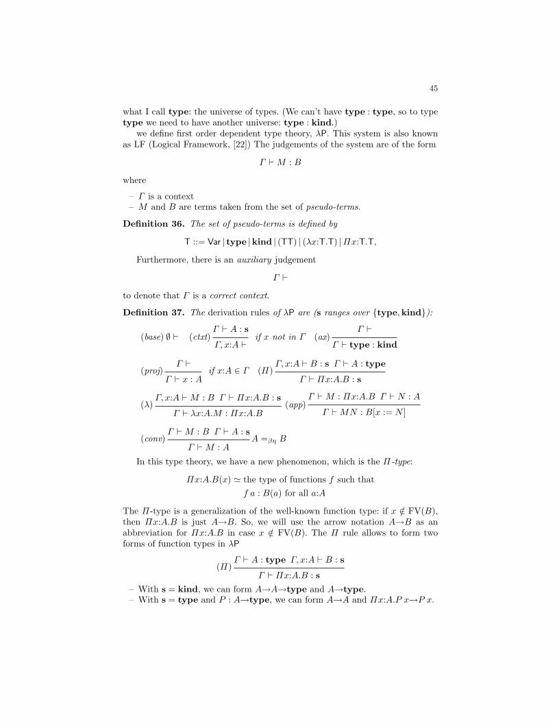
45

what I call type: the universe of types. (We can’t have type : type, so to typetype we need to have another universe: type : kind.)

we define first order dependent type theory, λP. This system is also knownas LF (Logical Framework, [22]) The judgements of the system are of the form

Γ `M : B

where

– Γ is a context– M and B are terms taken from the set of pseudo-terms.

Definition 36. The set of pseudo-terms is defined by

T ::= Var | type |kind | (TT) | (λx:T.T) |Πx:T.T,

Furthermore, there is an auxiliary judgement

Γ `

to denote that Γ is a correct context.

Definition 37. The derivation rules of λP are (s ranges over type,kind):

(base) ∅ ` (ctxt)Γ ` A : s

Γ, x:A `if x not in Γ (ax)

Γ `

Γ ` type : kind

(proj)Γ `

Γ ` x : Aif x:A ∈ Γ (Π)

Γ, x:A ` B : s Γ ` A : type

Γ ` Πx:A.B : s

(λ)Γ, x:A `M : B Γ ` Πx:A.B : s

Γ ` λx:A.M : Πx:A.B(app)

Γ `M : Πx:A.B Γ ` N : A

Γ `MN : B[x := N ]

(conv)Γ `M : B Γ ` A : s

Γ `M : AA =βη B

In this type theory, we have a new phenomenon, which is the Π-type:

Πx:A.B(x) ' the type of functions f such thatf a : B(a) for all a:A

The Π-type is a generalization of the well-known function type: if x /∈ FV(B),then Πx:A.B is just A→B. So, we will use the arrow notation A→B as anabbreviation for Πx:A.B in case x /∈ FV(B). The Π rule allows to form twoforms of function types in λP

(Π)Γ ` A : type Γ, x:A ` B : s

Γ ` Πx:A.B : s

– With s = kind, we can form A→A→type and A→type.– With s = type and P : A→type, we can form A→A and Πx:A.P x→P x.

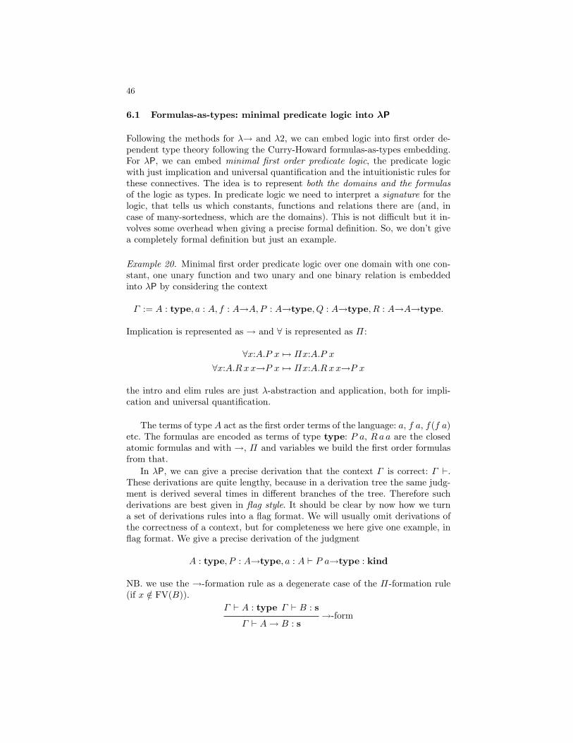
46

6.1 Formulas-as-types: minimal predicate logic into λP

Following the methods for λ→ and λ2, we can embed logic into first order de-pendent type theory following the Curry-Howard formulas-as-types embedding.For λP, we can embed minimal first order predicate logic, the predicate logicwith just implication and universal quantification and the intuitionistic rules forthese connectives. The idea is to represent both the domains and the formulasof the logic as types. In predicate logic we need to interpret a signature for thelogic, that tells us which constants, functions and relations there are (and, incase of many-sortedness, which are the domains). This is not difficult but it in-volves some overhead when giving a precise formal definition. So, we don’t givea completely formal definition but just an example.

Example 20. Minimal first order predicate logic over one domain with one con-stant, one unary function and two unary and one binary relation is embeddedinto λP by considering the context

Γ := A : type, a : A, f : A→A,P : A→type, Q : A→type, R : A→A→type.

Implication is represented as → and ∀ is represented as Π:

∀x:A.P x 7→ Πx:A.P x∀x:A.Rxx→P x 7→ Πx:A.Rxx→P x

the intro and elim rules are just λ-abstraction and application, both for impli-cation and universal quantification.

The terms of type A act as the first order terms of the language: a, f a, f(f a)etc. The formulas are encoded as terms of type type: P a, Raa are the closedatomic formulas and with →, Π and variables we build the first order formulasfrom that.

In λP, we can give a precise derivation that the context Γ is correct: Γ `.These derivations are quite lengthy, because in a derivation tree the same judg-ment is derived several times in different branches of the tree. Therefore suchderivations are best given in flag style. It should be clear by now how we turna set of derivations rules into a flag format. We will usually omit derivations ofthe correctness of a context, but for completeness we here give one example, inflag format. We give a precise derivation of the judgment

A : type, P : A→type, a : A ` P a→type : kind

NB. we use the →-formation rule as a degenerate case of the Π-formation rule(if x /∈ FV(B)).

Γ ` A : type Γ ` B : s→-form

Γ ` A→ B : s

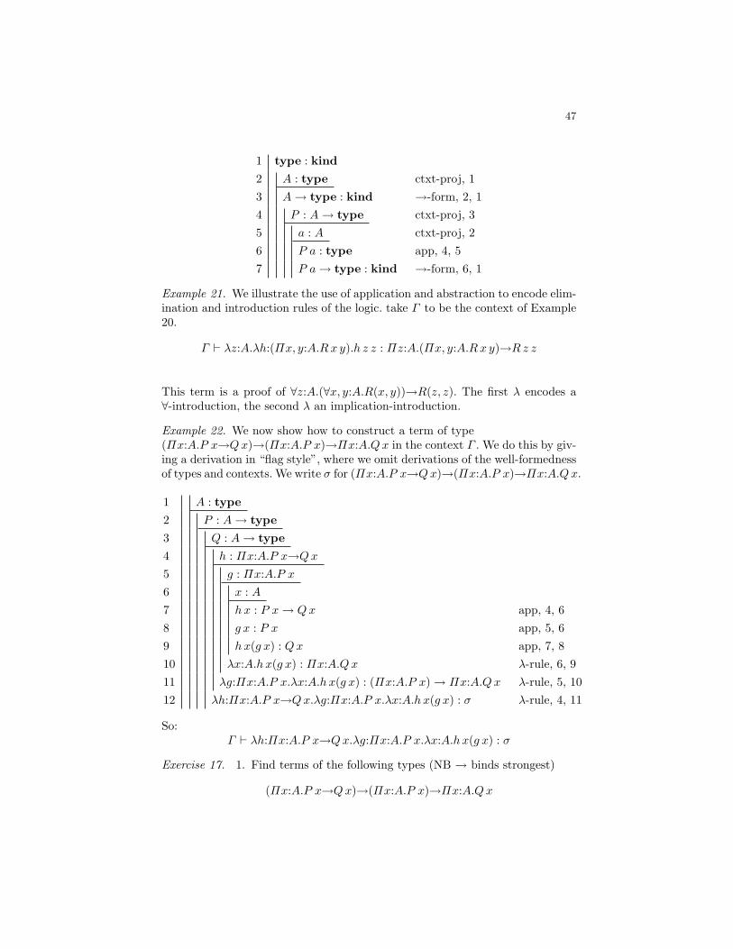
47

1 type : kind

2 A : type ctxt-proj, 13 A→ type : kind →-form, 2, 14 P : A→ type ctxt-proj, 35 a : A ctxt-proj, 26 P a : type app, 4, 57 P a→ type : kind →-form, 6, 1

Example 21. We illustrate the use of application and abstraction to encode elim-ination and introduction rules of the logic. take Γ to be the context of Example20.

Γ ` λz:A.λh:(Πx, y:A.Rx y).h z z : Πz:A.(Πx, y:A.Rx y)→Rz z

This term is a proof of ∀z:A.(∀x, y:A.R(x, y))→R(z, z). The first λ encodes a∀-introduction, the second λ an implication-introduction.

Example 22. We now show how to construct a term of type(Πx:A.P x→Qx)→(Πx:A.P x)→Πx:A.Qx in the context Γ . We do this by giv-ing a derivation in “flag style”, where we omit derivations of the well-formednessof types and contexts. We write σ for (Πx:A.P x→Qx)→(Πx:A.P x)→Πx:A.Qx.

1 A : type

2 P : A→ type

3 Q : A→ type

4 h : Πx:A.P x→Qx5 g : Πx:A.P x6 x : A7 hx : P x→ Qx app, 4, 68 g x : P x app, 5, 69 hx(g x) : Qx app, 7, 810 λx:A.hx(g x) : Πx:A.Qx λ-rule, 6, 911 λg:Πx:A.P x.λx:A.hx(g x) : (Πx:A.P x)→ Πx:A.Qx λ-rule, 5, 1012 λh:Πx:A.P x→Qx.λg:Πx:A.P x.λx:A.hx(g x) : σ λ-rule, 4, 11

So:Γ ` λh:Πx:A.P x→Qx.λg:Πx:A.P x.λx:A.hx(g x) : σ

Exercise 17. 1. Find terms of the following types (NB → binds strongest)

(Πx:A.P x→Qx)→(Πx:A.P x)→Πx:A.Qx

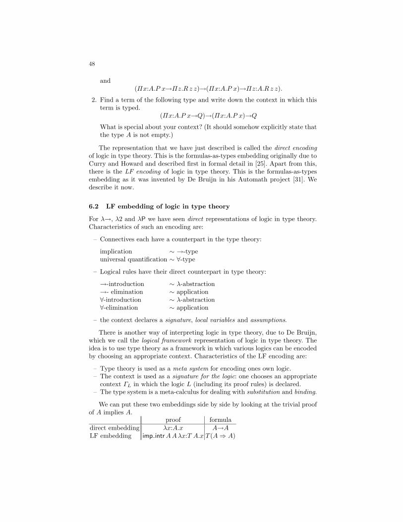
48

and(Πx:A.P x→Πz.R z z)→(Πx:A.P x)→Πz:A.R z z).

2. Find a term of the following type and write down the context in which thisterm is typed.

(Πx:A.P x→Q)→(Πx:A.P x)→Q

What is special about your context? (It should somehow explicitly state thatthe type A is not empty.)

The representation that we have just described is called the direct encodingof logic in type theory. This is the formulas-as-types embedding originally due toCurry and Howard and described first in formal detail in [25]. Apart from this,there is the LF encoding of logic in type theory. This is the formulas-as-typesembedding as it was invented by De Bruijn in his Automath project [31]. Wedescribe it now.

6.2 LF embedding of logic in type theory

For λ→, λ2 and λP we have seen direct representations of logic in type theory.Characteristics of such an encoding are:

– Connectives each have a counterpart in the type theory:

implication ∼ →-typeuniversal quantification ∼ ∀-type

– Logical rules have their direct counterpart in type theory:

→-introduction ∼ λ-abstraction→- elimination ∼ application∀-introduction ∼ λ-abstraction∀-elimination ∼ application

– the context declares a signature, local variables and assumptions.

There is another way of interpreting logic in type theory, due to De Bruijn,which we call the logical framework representation of logic in type theory. Theidea is to use type theory as a framework in which various logics can be encodedby choosing an appropriate context. Characteristics of the LF encoding are:

– Type theory is used as a meta system for encoding ones own logic.– The context is used as a signature for the logic: one chooses an appropriate

context ΓL in which the logic L (including its proof rules) is declared.– The type system is a meta-calculus for dealing with substitution and binding.

We can put these two embeddings side by side by looking at the trivial proofof A implies A.

proof formuladirect embedding λx:A.x A→ALF embedding imp intrAAλx:T A.x T (A⇒ A)

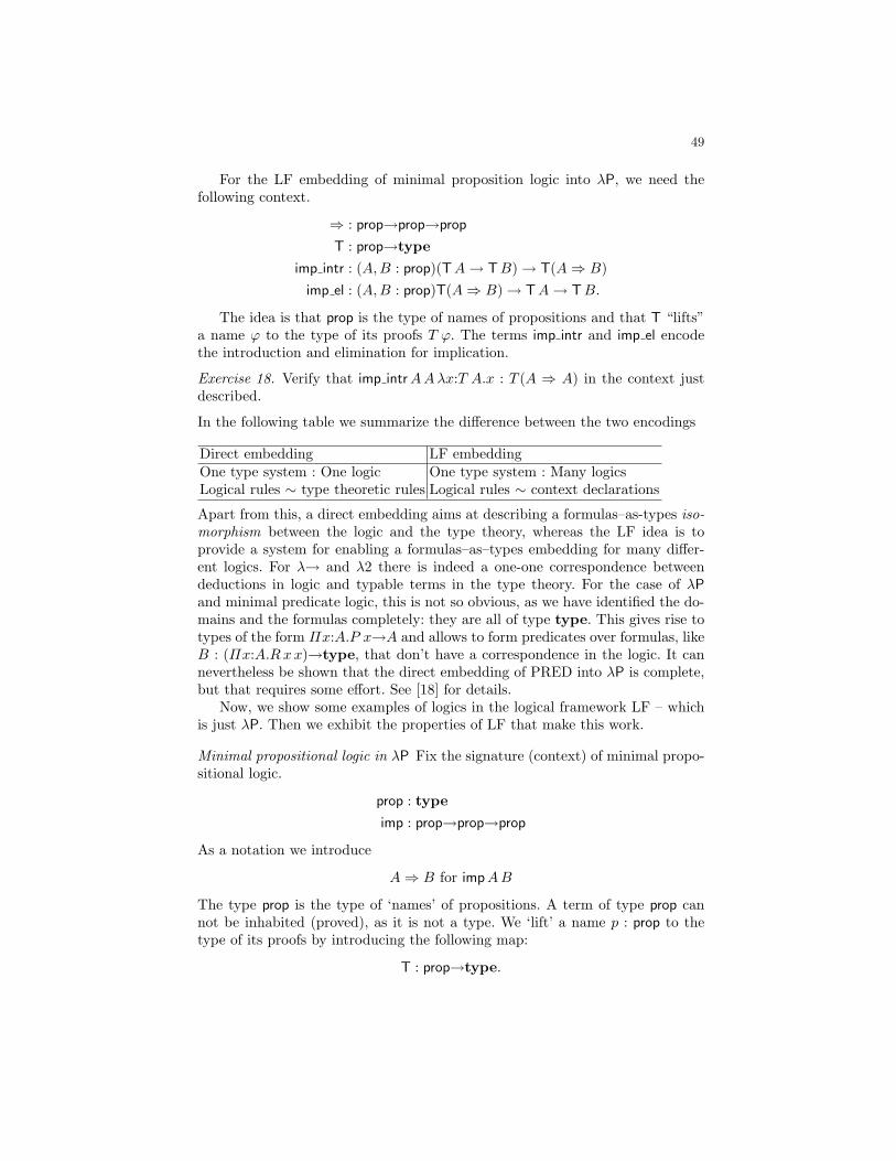
49

For the LF embedding of minimal proposition logic into λP, we need thefollowing context.

⇒ : prop→prop→prop

T : prop→type

imp intr : (A,B : prop)(TA→ TB)→ T(A⇒ B)imp el : (A,B : prop)T(A⇒ B)→ TA→ TB.

The idea is that prop is the type of names of propositions and that T “lifts”a name ϕ to the type of its proofs T ϕ. The terms imp intr and imp el encodethe introduction and elimination for implication.

Exercise 18. Verify that imp intrAAλx:T A.x : T (A ⇒ A) in the context justdescribed.

In the following table we summarize the difference between the two encodings

Direct embedding LF embeddingOne type system : One logic One type system : Many logicsLogical rules ∼ type theoretic rules Logical rules ∼ context declarations

Apart from this, a direct embedding aims at describing a formulas–as-types iso-morphism between the logic and the type theory, whereas the LF idea is toprovide a system for enabling a formulas–as–types embedding for many differ-ent logics. For λ→ and λ2 there is indeed a one-one correspondence betweendeductions in logic and typable terms in the type theory. For the case of λPand minimal predicate logic, this is not so obvious, as we have identified the do-mains and the formulas completely: they are all of type type. This gives rise totypes of the form Πx:A.P x→A and allows to form predicates over formulas, likeB : (Πx:A.Rxx)→type, that don’t have a correspondence in the logic. It cannevertheless be shown that the direct embedding of PRED into λP is complete,but that requires some effort. See [18] for details.

Now, we show some examples of logics in the logical framework LF – whichis just λP. Then we exhibit the properties of LF that make this work.

Minimal propositional logic in λP Fix the signature (context) of minimal propo-sitional logic.

prop : type

imp : prop→prop→prop

As a notation we introduce

A⇒ B for impAB

The type prop is the type of ‘names’ of propositions. A term of type prop cannot be inhabited (proved), as it is not a type. We ‘lift’ a name p : prop to thetype of its proofs by introducing the following map:

T : prop→type.

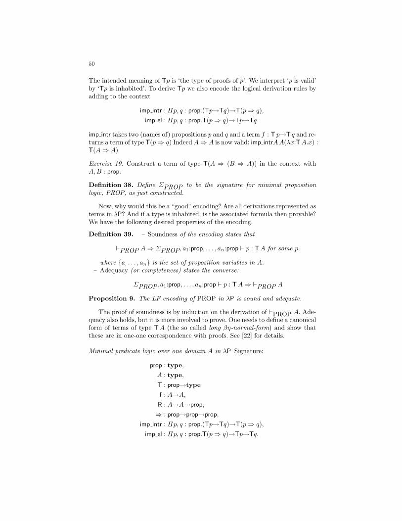
50

The intended meaning of Tp is ‘the type of proofs of p’. We interpret ‘p is valid’by ‘Tp is inhabited’. To derive Tp we also encode the logical derivation rules byadding to the context

imp intr : Πp, q : prop.(Tp→Tq)→T(p⇒ q),imp el : Πp, q : prop.T(p⇒ q)→Tp→Tq.

imp intr takes two (names of) propositions p and q and a term f : T p→T q and re-turns a term of type T(p⇒ q) IndeedA⇒ A is now valid: imp intrAA(λx:TA.x) :T(A⇒ A)

Exercise 19. Construct a term of type T(A ⇒ (B ⇒ A)) in the context withA,B : prop.

Definition 38. Define ΣPROP to be the signature for minimal propositionlogic, PROP, as just constructed.

Now, why would this be a “good” encoding? Are all derivations represented asterms in λP? And if a type is inhabited, is the associated formula then provable?We have the following desired properties of the encoding.

Definition 39. – Soundness of the encoding states that

`PROP A⇒ ΣPROP, a1:prop, . . . , an:prop ` p : TA for some p.

where a, . . . , an is the set of proposition variables in A.– Adequacy (or completeness) states the converse:

ΣPROP, a1:prop, . . . , an:prop ` p : TA⇒ `PROP A

Proposition 9. The LF encoding of PROP in λP is sound and adequate.

The proof of soundness is by induction on the derivation of `PROP A. Ade-quacy also holds, but it is more involved to prove. One needs to define a canonicalform of terms of type TA (the so called long βη-normal-form) and show thatthese are in one-one correspondence with proofs. See [22] for details.

Minimal predicate logic over one domain A in λP Signature:

prop : type,

A : type,

T : prop→type

f : A→A,R : A→A→prop,

⇒ : prop→prop→prop,

imp intr : Πp, q : prop.(Tp→Tq)→T(p⇒ q),imp el : Πp, q : prop.T(p⇒ q)→Tp→Tq.

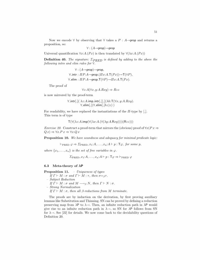
51

Now we encode ∀ by observing that ∀ takes a P : A→prop and returns aproposition, so:

∀ : (A→prop)→prop

Universal quantification ∀x:A.(Px) is then translated by ∀(λx:A.(Px))

Definition 40. The signature: ΣPRED is defined by adding to the above thefollowing intro and elim rules for ∀.

∀ : (A→prop)→prop,

∀ intr : ΠP :A→prop.(Πx:A.T(Px))→T(∀P ),∀ elim : ΠP :A→prop.T(∀P )→Πx:A.T(Px).

The proof of∀z:A(∀x, y:A.Rxy)⇒ Rzz

is now mirrored by the proof-term

∀ intr[ ]( λz:A.imp intr[ ][ ](λh:T(∀x, y:A.Rxy).∀ elim[ ](∀ elim[ ]hz)z) )

For readability, we have replaced the instantiations of the Π-type by [ ].This term is of type

T(∀(λz:A.imp(∀(λx:A.(∀(λy:A.Rxy))))(Rzz)))

Exercise 20. Construct a proof-term that mirrors the (obvious) proof of ∀x(P x⇒Qx)⇒ ∀x.P x⇒ ∀x.Qx

Proposition 10. We have soundness and adequacy for minimal predicate logic:

`PRED ϕ⇒ ΣPRED, x1:A, . . . , xn:A ` p : Tϕ, for some p,

where x1, . . . , xn is the set of free variables in ϕ.

ΣPRED, x1:A, . . . , xn:A ` p : Tϕ⇒ `PRED ϕ

6.3 Meta-theory of λP

Proposition 11. – Uniqueness of typesIf Γ `M : σ and Γ `M : τ , then σ=βτ .

– Subject ReductionIf Γ `M : σ and M −→β N , then Γ ` N : σ.

– Strong NormalizationIf Γ `M : σ, then all β-reductions from M terminate.

The proofs are by induction on the derivation, by first proving auxiliarylemmas like Substitution and Thinning. SN can be proved by defining a reductionpreserving map from λP to λ→. Then, an infinite reduction path in λP wouldgive rise to an infinite reduction path in λ→, so SN for λP follows from SNfor λ→. See [22] for details. We now come back to the decidability questions ofDefinition 20.

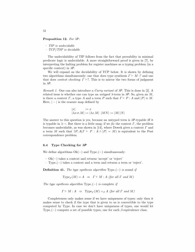
52

Proposition 12. For λP:

– TIP is undecidable– TCP/TSP is decidable

The undecidability of TIP follows from the fact that provability in minimalpredicate logic is undecidable. A more straightforward proof is given in [7], byinterpreting the halting problem for register machines as a typing problem (in aspecific context) in λP.

We will expand on the decidability of TCP below. It is shown by definingtwo algorithms simultaneously: one that does type synthesis Γ ` M :? and onethat does context checking: Γ `?. This is to mirror the two forms of judgmentin λP.

Remark 1. One can also introduce a Curry variant of λP. This is done in [2]. Arelated issue is whether one can type an untyped λ-term in λP. So, given an M ,is there a context Γ , a type A and a term P such that Γ ` P : A and |P | ≡M .Here, | − | is the erasure map defined by

|x| := x|λx:σ.M | := |λx.M | |MN | := |M | |N |

The answer to this question is yes, because an untyped term is λP-typable iff itis typable in λ→. But there is a little snag: if we fix the context Γ , the problembecomes undecidable, as was shown in [14], where Dowek gives a context Γ anda term M such that ∃P,A(Γ ` P : A ∧ |P | = M) is equivalent to the Postcorrespondence problem.

6.4 Type Checking for λP

We define algorithms Ok(−) and Type (−) simultaneously:

– Ok(−) takes a context and returns ‘accept’ or ‘reject’– Type (−) takes a context and a term and returns a term or ‘reject’.

Definition 41. The type synthesis algorithm Type (−) is sound if

TypeΓ (M) = A ⇒ Γ `M : A (for all Γ and M)

The type synthesis algorithm Type (−) is complete if

Γ `M : A ⇒ TypeΓ (M) =β A (for all Γ and M)

Completeness only makes sense if we have uniqueness of types: only then itmakes sense to check if the type that is given to us is convertible to the typecomputed by Type. In case we don’t have uniqueness of types, one would letType (−) compute a set of possible types, one for each β-equivalence class.

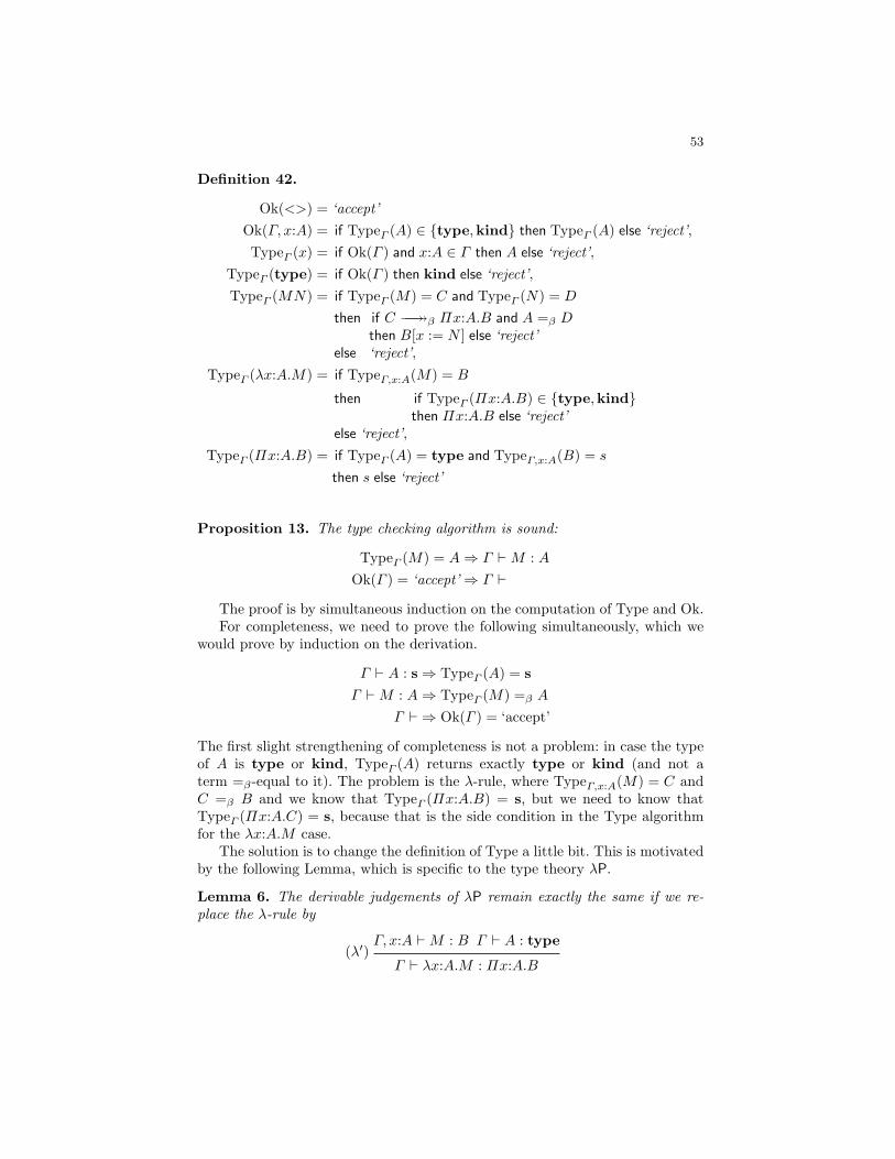
53

Definition 42.

Ok(<>) = ‘accept’Ok(Γ, x:A) = if TypeΓ (A) ∈ type,kind then TypeΓ (A) else ‘reject’,TypeΓ (x) = if Ok(Γ ) and x:A ∈ Γ then A else ‘reject’,

TypeΓ (type) = if Ok(Γ ) then kind else ‘reject’,TypeΓ (MN) = if TypeΓ (M) = C and TypeΓ (N) = D

then if C −→−→β Πx:A.B and A =β Dthen B[x := N ] else ‘reject’

else ‘reject’,TypeΓ (λx:A.M) = if TypeΓ,x:A(M) = B

then if TypeΓ (Πx:A.B) ∈ type,kindthen Πx:A.B else ‘reject’

else ‘reject’,TypeΓ (Πx:A.B) = if TypeΓ (A) = type and TypeΓ,x:A(B) = s

then s else ‘reject’

Proposition 13. The type checking algorithm is sound:

TypeΓ (M) = A⇒ Γ `M : AOk(Γ ) = ‘accept’⇒ Γ `

The proof is by simultaneous induction on the computation of Type and Ok.For completeness, we need to prove the following simultaneously, which we

would prove by induction on the derivation.

Γ ` A : s⇒ TypeΓ (A) = s

Γ `M : A⇒ TypeΓ (M) =β A

Γ ` ⇒ Ok(Γ ) = ‘accept’

The first slight strengthening of completeness is not a problem: in case the typeof A is type or kind, TypeΓ (A) returns exactly type or kind (and not aterm =β-equal to it). The problem is the λ-rule, where TypeΓ,x:A(M) = C andC =β B and we know that TypeΓ (Πx:A.B) = s, but we need to know thatTypeΓ (Πx:A.C) = s, because that is the side condition in the Type algorithmfor the λx:A.M case.

The solution is to change the definition of Type a little bit. This is motivatedby the following Lemma, which is specific to the type theory λP.

Lemma 6. The derivable judgements of λP remain exactly the same if we re-place the λ-rule by

(λ′)Γ, x:A `M : B Γ ` A : type

Γ ` λx:A.M : Πx:A.B

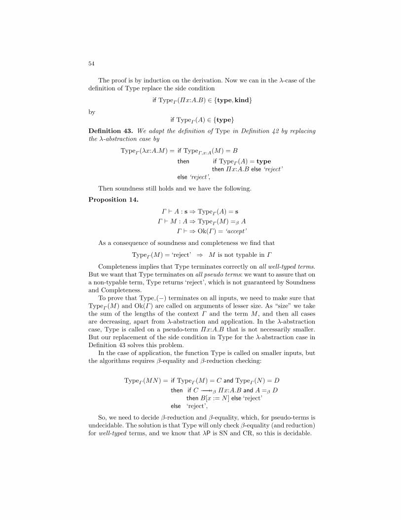
54

The proof is by induction on the derivation. Now we can in the λ-case of thedefinition of Type replace the side condition

if TypeΓ (Πx:A.B) ∈ type,kind

byif TypeΓ (A) ∈ type

Definition 43. We adapt the definition of Type in Definition 42 by replacingthe λ-abstraction case by

TypeΓ (λx:A.M) = if TypeΓ,x:A(M) = B

then if TypeΓ (A) = typethen Πx:A.B else ‘reject’

else ‘reject’,

Then soundness still holds and we have the following.

Proposition 14.

Γ ` A : s⇒ TypeΓ (A) = s

Γ `M : A⇒ TypeΓ (M) =β A

Γ ` ⇒ Ok(Γ ) = ‘accept’

As a consequence of soundness and completeness we find that

TypeΓ (M) = ‘reject’ ⇒ M is not typable in Γ

Completeness implies that Type terminates correctly on all well-typed terms.But we want that Type terminates on all pseudo terms: we want to assure that ona non-typable term, Type returns ‘reject’, which is not guaranteed by Soundnessand Completeness.

To prove that Type (−) terminates on all inputs, we need to make sure thatTypeΓ (M) and Ok(Γ ) are called on arguments of lesser size. As “size” we takethe sum of the lengths of the context Γ and the term M , and then all casesare decreasing, apart from λ-abstraction and application. In the λ-abstractioncase, Type is called on a pseudo-term Πx:A.B that is not necessarily smaller.But our replacement of the side condition in Type for the λ-abstraction case inDefinition 43 solves this problem.

In the case of application, the function Type is called on smaller inputs, butthe algorithms requires β-equality and β-reduction checking:

TypeΓ (MN) = if TypeΓ (M) = C and TypeΓ (N) = D

then if C −→−→β Πx:A.B and A =β Dthen B[x := N ] else ‘reject’

else ‘reject’,

So, we need to decide β-reduction and β-equality, which, for pseudo-terms isundecidable. The solution is that Type will only check β-equality (and reduction)for well-typed terms, and we know that λP is SN and CR, so this is decidable.

55

Proposition 15. Termination of Type and Ok: For all pseudo-terms M andpseudo-contexts Γ , TypeΓ (M) terminates (in either a pseudo-term A or ‘reject’)and Ok(Γ ) terminates (in either ‘accept’ or ‘reject’).

The proof is by induction on the size of the inputs, using the Soundness(Proposition 13) and decidability of β-equality for well-typed terms in the ap-plication case.

7 Conclusion and further reading

In this paper we have introduced various type theories by focussing on the Curry-Howard formulas-as-types embedding and by highlighting some of the program-ming aspects related to type theory. As stated in the Introduction, we could havepresented the type systems a la Church in a unified framework of the “λ-cube”or “Pure Type Systems”, but for expository reasons we have refrained from do-ing so. In the PTS framework, one can study the systems Fω, a higher orderextension of system F , λHOL, a type systems for higher order (predicate) logic,and the Calculus of Constructions, a higher order extension of λP. Also one cangeneralize these systems to the logically inconsistent systems λU and λ? wheretype is itself a type. (These systems are computationally not inconsistent sostill interesting to study.) We refer to [4, 5] and the references in those papersfor further reading.

In another direction, there are various typing constructs that can be addedto make the theories more powerful. The most prominent one is the addition ofa scheme for inductive types, which also adds an induction and a well-foundedrecursion principle for every inductive type. Examples are the Calculus of Induc-tive Constructions (CIC) and Martin-Lof type theory. The latter is introducedin the paper by Bove and Dybjer and a good reference is [32]. CIC is the typetheory implemented in the proof assistant Coq and a good reference for boththe theory and the tool is [6].

In the direction of programming, there is a world of literature and a goodstarting point is [33]. We have already mentioned PCF [35], which is the simplestway to turn λ→ into a Turing complete language. The next thing to add arealgebraic data types, which are the programmer’s analogue to inductive types.Using these one can define and compute with data types of lists, trees etc. as aprimitive in the language (as opposed to coding them in λ2 as we have done inSection 5.5). Other important concepts to add, especially to the type systems ala Curry, are overloading and subtyping. A good reference for further reading is[33].

References

1. E.S. Bainbridge, P.J. Freyd, A. Scedrov, and P.J. Scott, Functorialpolymorphism. Theoretical Computer Science 70, 35-64, 1990.

56

2. S. van Bakel, L. Liquori, S. Ronchi Della Rocca and P. Urzyczyn, ComparingCubes of Typed and Type Assignment Systems. Ann. Pure Appl. Logic 86(3):267-303, 1997.

3. H. Barendregt, The Lambda Calculus: Its Syntax and Semantics, vol. 103 ofStudies in Logic and the Foundations of Mathematics, North Holland, 1981.

4. H. Barendregt and H. Geuvers, Proof Assistants using Dependent Type Systems,Chapter 18 of the Handbook of Automated Reasoning (Vol 2), eds. A. Robinsonand A. Voronkov, Elsevier, pp. 1149 – 1238, 2001.

5. H. Barendregt, Lambda Calculi with Types, Handbook of Logic in ComputerScience, Volume 1, Abramsky, Gabbay, Maibaum (Eds.), Clarendon, 1992.

6. Y. Bertot and P. Casteran, Interactive Theorem Proving and ProgramDevelopment: Coq’Art : the Calculus of Inductive Constructions, EATCS Series:Texts in Theoretical Computer Science, Springer 2004, 469 pp.

7. M. Bezem and J. Springintveld, A Simple Proof of the Undecidability ofInhabitation in λP . J. Funct. Program. 6(5): 757-761, 1996.

8. C. Bohm and A. Berarducci, Automatic synthesis of typed λ-programs on termalgebras, Theoretical Computer Science 39, pp. 135154, 1985.

9. A. Church, A formulation of the simple theory of types, Journal of SymbolicLogic 5, pp. 5668, 1940.

10. R.L Constable, S.F. Allen, H.M. Bromley, W.R. Cleaveland, J.F. Cremer, R.W.Harper, D.J. Howe, T.B. Knoblock, N.P. Mendler, P. Panangaden, J.T. Sasakiand S.F. Smith, Implementing Mathematics with the Nuprl Development System,Prentice-Hall, NJ, 1986.

11. H.B. Curry, R. Feys, and W. Craig, Combinatory Logic, Vol. 1. North–Holland,Amsterdam, 1958.

12. L. Damas and R. Milner, Principal type-schemes for functional programs, POPL’82: Proceedings of the 9th ACM SIGPLAN-SIGACT symposium on Principles ofprogramming languages, pp. 207-212, ACM, 1982.

13. M. Davis, editor, The Undecidable, Basic Papers on Undecidable Propositions,Unsolvable Problems And Computable Functions, Raven Press, New York, 1965.

14. G. Dowek, The Undecidability of Typability in the Lambda-Pi-CalculusProceedings of the International Conference on Typed Lambda Calculi andApplications, LNCS 664, pp. 139 - 145, 1993.

15. G. Dowek, Collections, sets and types, Mathematical Structures in ComputerScience 9, pp. 1-15, 1999.

16. F. Fitch, Symbolic Logic, An Introduction, The Ronald Press Company, 1952.17. R.O. Gandy, An early proof of normalization by A.M. Turing. In J.P. Seldin and

J.R. Hindley, editors, to H.B. Curry: Essays on Combinatory Logic, LambdaCalculus and Formalism, pages 453455. Academic Press, 1980.

18. H. Geuvers and E. Barendsen, Some logical and syntactical observationsconcerning the first order dependent type system λP , Math. Struc. in Comp. Sci.vol. 9-4, 1999, pp. 335 – 360.

19. J.-Y. Girard, P. Taylor, and Y. Lafont, Proofs and types. Cambridge tracts intheoretical computer science, no. 7. Cambridge University Press.

20. J.-Y. Girard, The system F of variable types, fifteen years later. TheoreticalComputer Science, 45:159192, 1986.

21. J.-Y. Girard, Une extension de l’interpretation de Godel a l’analyse et sonapplication a l’elimination des coupures dans l’analyse et la theorie des types,Proceedings of the Second Scandinavian Logic Symposium, pp. 63–92. Studies inLogic and the Foundations of Mathematics, Vol. 63, North-Holland, Amsterdam,1971.

57

22. R. Harper, F. Honsell and G. Plotkin, A Framework for Defining Logics,Proceedings 2nd Annual IEEE Symp. on Logic in Computer Science, LICS’87,Ithaca, NY, USA, 22–25 June 1987

23. J.R. Hindley, The principal type-scheme of an object in combinatory logic,Transactions of the American Mathematical Society 146 (1969), 29–60.

24. J.R. Hindley and J.P. Seldin, Introduction to combinators and lambda-calculus.London Mathematical Society Student Texts. Cambridge University Press, 1986.

25. W. Howard, The formulas-as-types notion of construction. In J.P. Seldin and J.R.Hindley, editors, To H.B. Curry: Essays on Combinatory Logic, Lambda-Calculusand Formalism, pages 479–490. Academic Press, NY, 1980.

26. F. Joachimski, R. Matthes, Short proofs of normalization for the simply- typedlambda-calculus, permutative conversions and Godel’s T. Arch. Math. Log. 42(1):59-87, 2003.

27. J. Lambek and P. Scott, Introduction to Higher Order Categorical Logic,Cambridge University Press, 1986.

28. P. Martin-Lof, Intuitionistic type theory, Bibliopolis, 1984.29. R. Milner, Robin, A Theory of Type Polymorphism in Programming, JCSS 17:

348-375, 1978.30. A. Mycroft, Polymorphic type schemes and recursive definitions, International

Symposium on Programming, LNCS 167, pp. 217-228, Springer 1984.31. R. Nederpelt, H. Geuvers and R. de Vrijer (eds.) Selected Papers on Automath,

Studies in Logic, Vol. 133, North-Holland, 1994.32. B. Nordstrom, K. Petersson and J. Smith, Programming in Martin-Lof ’s Type

Theory, An Introduction, Oxford University Press, 1990.33. Benjamin C. Pierce, Types and Programming Languages, MIT Press, 2002.34. G. Plotkin, Call-by-Name, Call-by-Value and the lambda-Calculus. Theor. Comp.

Sci. 1(2): 125-159, 1975.35. G. Plotkin, LCF considered as a programming language, Theor. Comp. Sci. 5,

pp. 223255, 1977.36. J.C. Reynolds, Polymorphism is not Set-Theoretic. In G. Kahn, D.B. MacQueen,

G. Plotkin (Eds.): Semantics of Data Types, International Symposium,Sophia-Antipolis, France, June 27-29, LNCS 173, Springer 1984, pp. 145-156.

37. H. Schwichtenberg, Definierbare Funktionen im λ-Kalkul mit Typen, Archiv furMathematische Logik und Grundlagenforschung 17, pp. 113114, 1976.

38. W.W. Tait, Intensional interpretation of functionals of finite type. J. Symbol.Logic, v. 32, n. 2, pages 187–199, 1967.

39. P. Urzyczyn and M. Sørensen, Lectures on the Curry-Howard Isomorphism,Volume 149 of Studies in Logic and the Foundations of Mathematics, Elsevier,2006.

40. M. Wand, A simple algorithm and proof for type inference,FundamentaInformaticae X, pp. 115122, 1987.

41. J.B Wells, Typability and type-checking in the second-order λ-calculus areequivalent and undecidable, Proceedings of the 9th Annual Symposium on Logicin Computer Science, Paris, France, IEEE Computer Society Press, pp. 176185,1994.