Introduction to Time Series Analysis. Lecture 14.

Last lecture: Maximum likelihood estimation

1. Review: Maximum likelihood estimation

2. Model selection

3. Integrated ARMA models

4. Seasonal ARMA

5. Seasonal ARIMA models

1

Recall: Maximum likelihood estimation

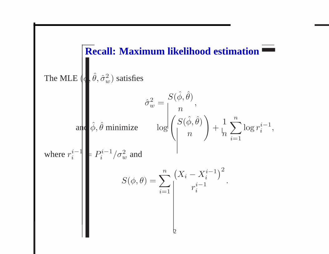
The MLE (φ̂, θ̂, σ̂2w) satisfies

σ̂2w =

S(φ̂, θ̂)

n,

andφ̂, θ̂ minimize log

(

S(φ̂, θ̂)

n

)

+1

n

n∑

i=1

log ri−1

i ,

whereri−1

i = P i−1

i /σ2w and

S(φ, θ) =n∑

i=1

(Xi −Xi−1

i

)2

ri−1

i

.

2

Recall: Maximum likelihood estimation

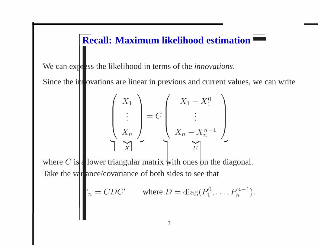
We can express the likelihood in terms of theinnovations.

Since the innovations are linear in previous and current values, we can write

X1

...

Xn

︸ ︷︷ ︸

X

= C

X1 −X01

...

Xn −Xn−1n

︸ ︷︷ ︸

U

whereC is a lower triangular matrix with ones on the diagonal.

Take the variance/covariance of both sides to see that

Γn = CDC ′ whereD = diag(P 01 , . . . , P

n−1n ).

3

Recall: Maximum likelihood estimation

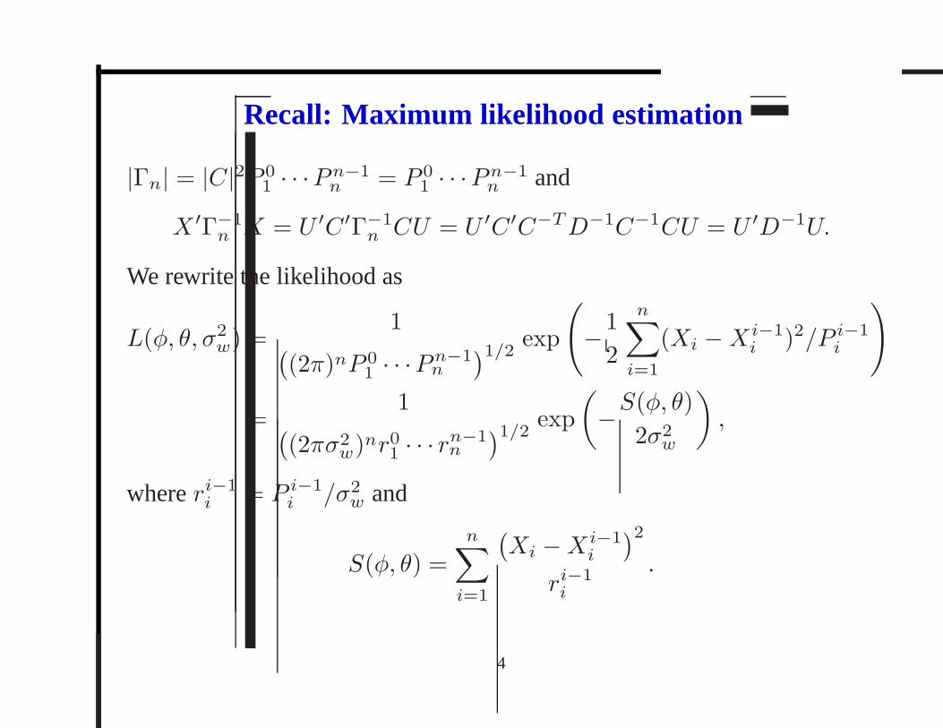
|Γn| = |C|2P 01 · · ·Pn−1

n = P 01 · · ·Pn−1

n and

X ′Γ−1n X = U ′C ′Γ−1

n CU = U ′C ′C−TD−1C−1CU = U ′D−1U.

We rewrite the likelihood as

L(φ, θ, σ2w) =

1((2π)nP 0

1 · · ·Pn−1n

)1/2exp

(

−1

2

n∑

i=1

(Xi −Xi−1

i )2/P i−1

i

)

=1

((2πσ2

w)nr01 · · · r

n−1n

)1/2exp

(

−S(φ, θ)

2σ2w

)

,

whereri−1

i = P i−1

i /σ2w and

S(φ, θ) =n∑

i=1

(Xi −Xi−1

i

)2

ri−1

i

.

4

Recall: Maximum likelihood estimation

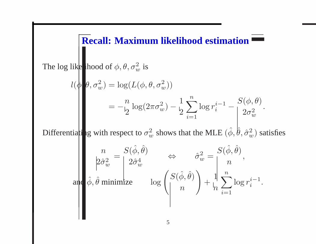
The log likelihood ofφ, θ, σ2w is

l(φ, θ, σ2w) = log(L(φ, θ, σ2

w))

= −n

2log(2πσ2

w)−1

2

n∑

i=1

log ri−1

i −S(φ, θ)

2σ2w

.

Differentiating with respect toσ2w shows that the MLE(φ̂, θ̂, σ̂2

w) satisfies

n

2σ̂2w

=S(φ̂, θ̂)

2σ̂4w

⇔ σ̂2w =

S(φ̂, θ̂)

n,

andφ̂, θ̂ minimize log

(

S(φ̂, θ̂)

n

)

+1

n

n∑

i=1

log ri−1

i .

5

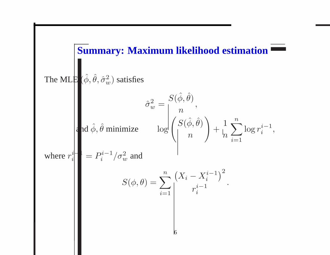
Summary: Maximum likelihood estimation

The MLE (φ̂, θ̂, σ̂2w) satisfies

σ̂2w =

S(φ̂, θ̂)

n,

andφ̂, θ̂ minimize log

(

S(φ̂, θ̂)

n

)

+1

n

n∑

i=1

log ri−1

i ,

whereri−1

i = P i−1

i /σ2w and

S(φ, θ) =

n∑

i=1

(Xi −Xi−1

i

)2

ri−1

i

.

6

Introduction to Time Series Analysis. Lecture 14.

1. Review: Maximum likelihood estimation

2. Model selection

3. Integrated ARMA models

4. Seasonal ARMA

5. Seasonal ARIMA models

7

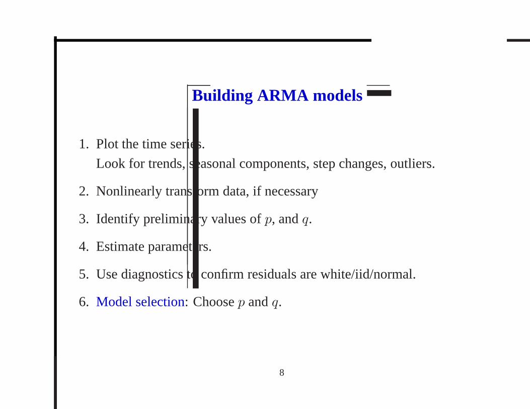
Building ARMA models

1. Plot the time series.

Look for trends, seasonal components, step changes, outliers.

2. Nonlinearly transform data, if necessary

3. Identify preliminary values ofp, andq.

4. Estimate parameters.

5. Use diagnostics to confirm residuals are white/iid/normal.

6. Model selection: Choosep andq.

8

Model Selection

We have used the datax to estimate parameters of several models. They all

fit well (the innovations are white). We need to choose a single model to

retain for forecasting. How do we do it?

If we had access to independent datay from the same process, we could

compare the likelihood on the new data,Ly(φ̂, θ̂, σ̂2w).

We could obtainy by leaving out some of the data from our model-building,

and reserving it for model selection. This is calledcross-validation. It

suffers from the drawback that we are not using all of the datafor parameter

estimation.

9

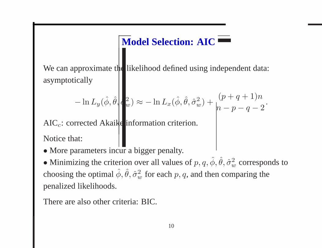
Model Selection: AIC

We can approximate the likelihood defined using independentdata:

asymptotically

− lnLy(φ̂, θ̂, σ̂2w) ≈ − lnLx(φ̂, θ̂, σ̂

2w) +

(p+ q + 1)n

n− p− q − 2.

AICc: corrected Akaike information criterion.

Notice that:

• More parameters incur a bigger penalty.

• Minimizing the criterion over all values ofp, q, φ̂, θ̂, σ̂2w corresponds to

choosing the optimal̂φ, θ̂, σ̂2w for eachp, q, and then comparing the

penalized likelihoods.

There are also other criteria: BIC.

10

Introduction to Time Series Analysis. Lecture 14.

1. Review: Maximum likelihood estimation

2. Computational simplifications: un/conditional least squares

3. Diagnostics

4. Model selection

5. Integrated ARMA models

6. Seasonal ARMA

7. Seasonal ARIMA models

11

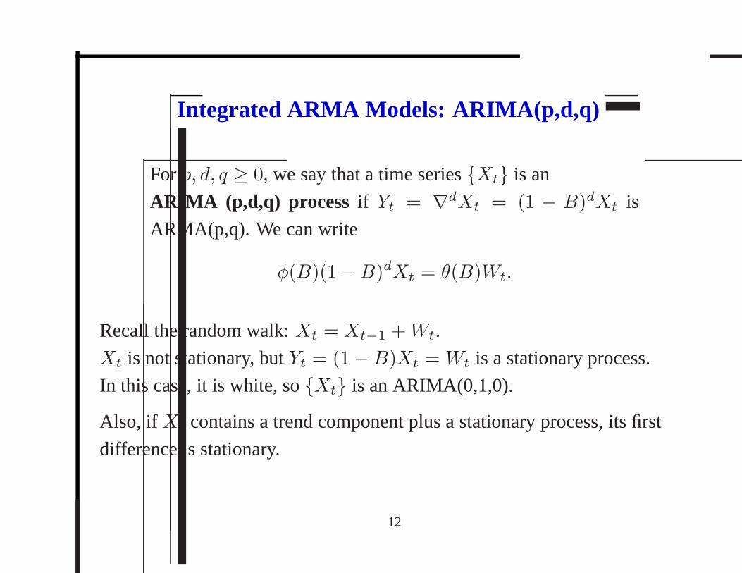
Integrated ARMA Models: ARIMA(p,d,q)

Forp, d, q ≥ 0, we say that a time series{Xt} is an

ARIMA (p,d,q) process if Yt = ∇dXt = (1 − B)dXt is

ARMA(p,q). We can write

φ(B)(1−B)dXt = θ(B)Wt.

Recall the random walk:Xt = Xt−1 +Wt.

Xt is not stationary, butYt = (1−B)Xt = Wt is a stationary process.

In this case, it is white, so{Xt} is an ARIMA(0,1,0).

Also, if Xt contains a trend component plus a stationary process, its first

difference is stationary.

12

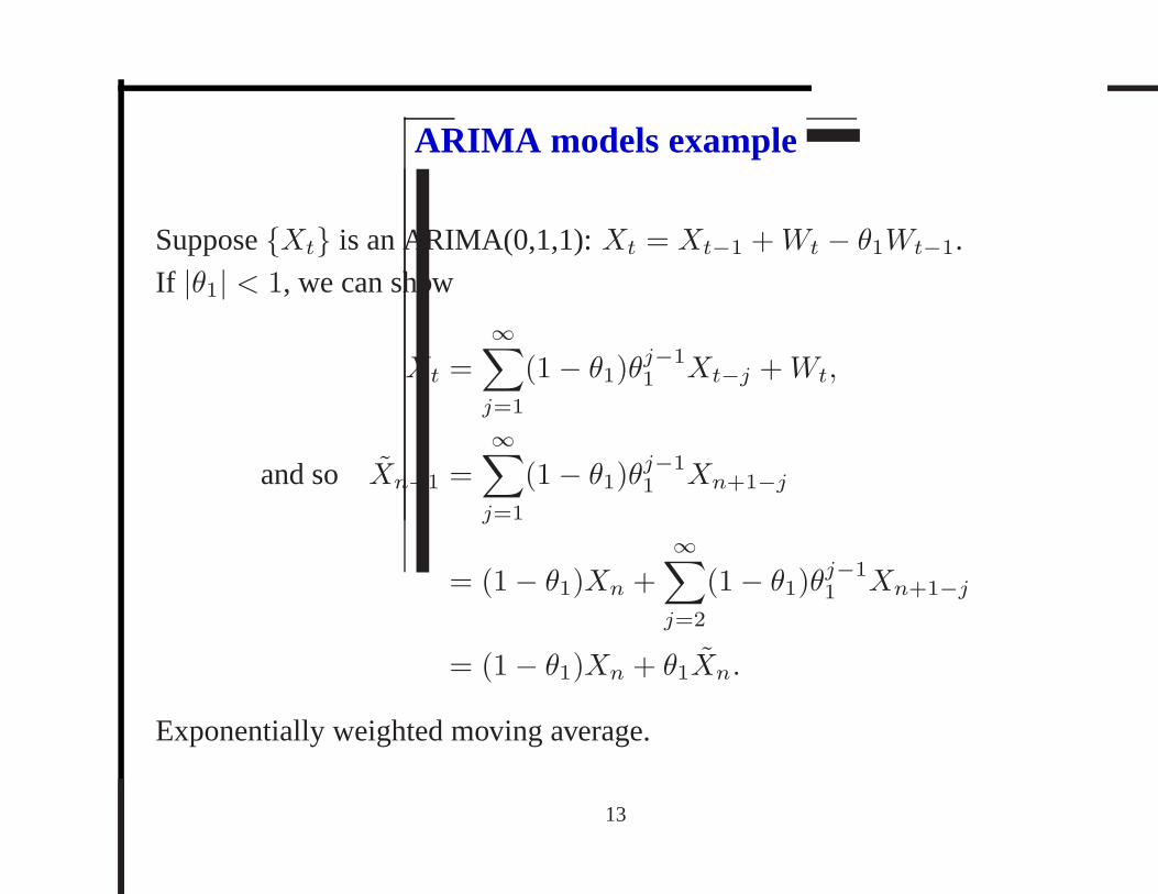
ARIMA models example

Suppose{Xt} is an ARIMA(0,1,1):Xt = Xt−1 +Wt − θ1Wt−1.

If |θ1| < 1, we can show

Xt =∞∑

j=1

(1− θ1)θj−1

1 Xt−j +Wt,

and so X̃n+1 =∞∑

j=1

(1− θ1)θj−1

1 Xn+1−j

= (1− θ1)Xn +

∞∑

j=2

(1− θ1)θj−1

1 Xn+1−j

= (1− θ1)Xn + θ1X̃n.

Exponentially weighted moving average.

13

Introduction to Time Series Analysis. Lecture 14.

1. Review: Maximum likelihood estimation

2. Computational simplifications: un/conditional least squares

3. Diagnostics

4. Model selection

5. Integrated ARMA models

6. Seasonal ARMA

7. Seasonal ARIMA models

14

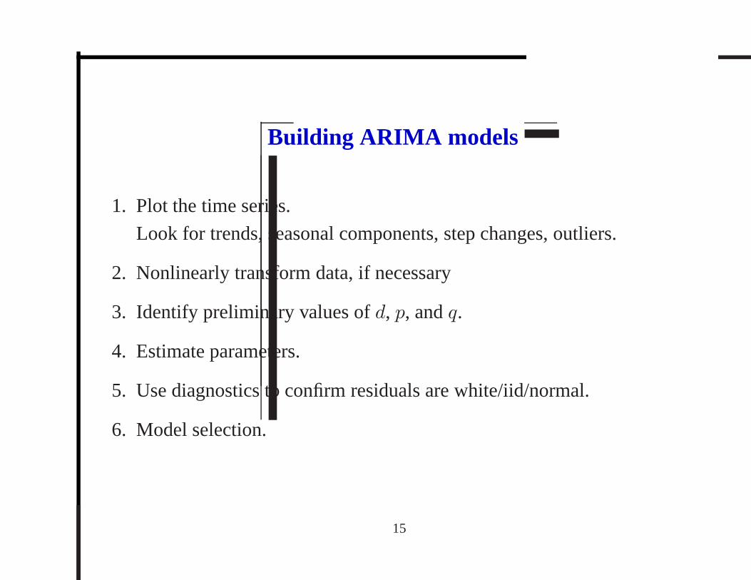
Building ARIMA models

1. Plot the time series.

Look for trends, seasonal components, step changes, outliers.

2. Nonlinearly transform data, if necessary

3. Identify preliminary values ofd, p, andq.

4. Estimate parameters.

5. Use diagnostics to confirm residuals are white/iid/normal.

6. Model selection.

15

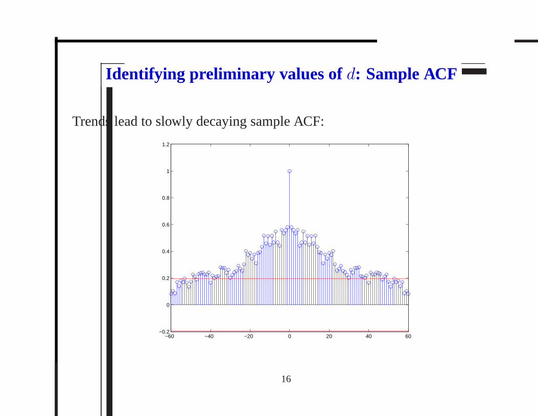
Identifying preliminary values of d: Sample ACF

Trends lead to slowly decaying sample ACF:

−60 −40 −20 0 20 40 60−0.2

0

0.2

0.4

0.6

0.8

1

1.2

16

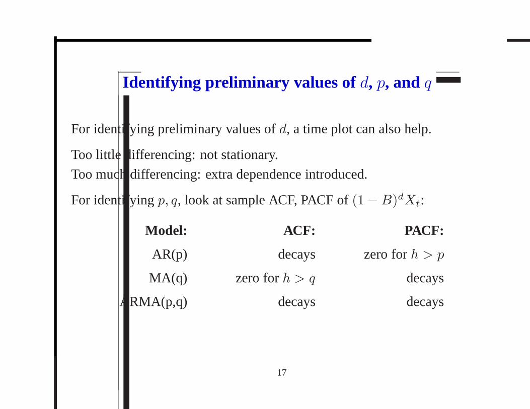
Identifying preliminary values of d, p, and q

For identifying preliminary values ofd, a time plot can also help.

Too little differencing: not stationary.

Too much differencing: extra dependence introduced.

For identifyingp, q, look at sample ACF, PACF of(1−B)dXt:

Model: ACF: PACF:

AR(p) decays zero forh > p

MA(q) zero forh > q decays

ARMA(p,q) decays decays

17

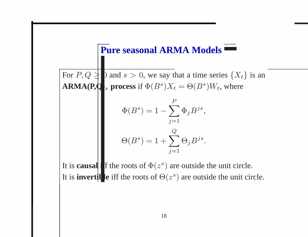
Pure seasonal ARMA Models

ForP,Q ≥ 0 ands > 0, we say that a time series{Xt} is an

ARMA(P,Q)s process if Φ(Bs)Xt = Θ(Bs)Wt, where

Φ(Bs) = 1−

P∑

j=1

ΦjBjs,

Θ(Bs) = 1 +

Q∑

j=1

ΘjBjs.

It is causal iff the roots ofΦ(zs) are outside the unit circle.

It is invertible iff the roots ofΘ(zs) are outside the unit circle.

18

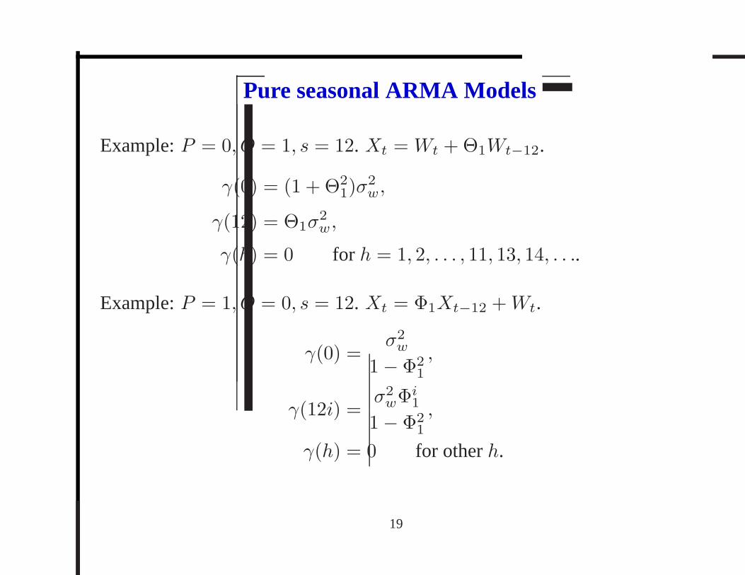
Pure seasonal ARMA Models

Example:P = 0, Q = 1, s = 12. Xt = Wt +Θ1Wt−12.

γ(0) = (1 + Θ21)σ

2w,

γ(12) = Θ1σ2w,

γ(h) = 0 for h = 1, 2, . . . , 11, 13, 14, . . ..

Example:P = 1, Q = 0, s = 12. Xt = Φ1Xt−12 +Wt.

γ(0) =σ2w

1− Φ21

,

γ(12i) =σ2wΦ

i1

1− Φ21

,

γ(h) = 0 for otherh.

19

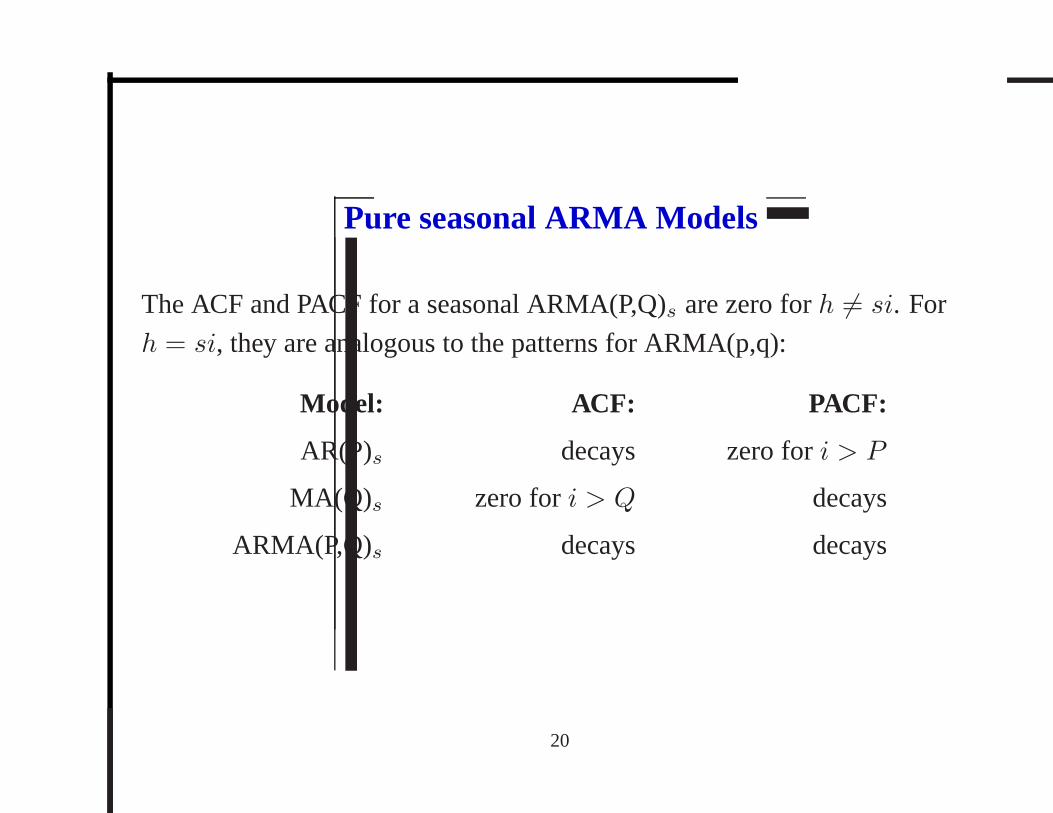
Pure seasonal ARMA Models

The ACF and PACF for a seasonal ARMA(P,Q)s are zero forh 6= si. For

h = si, they are analogous to the patterns for ARMA(p,q):

Model: ACF: PACF:

AR(P)s decays zero fori > P

MA(Q)s zero fori > Q decays

ARMA(P,Q)s decays decays

20

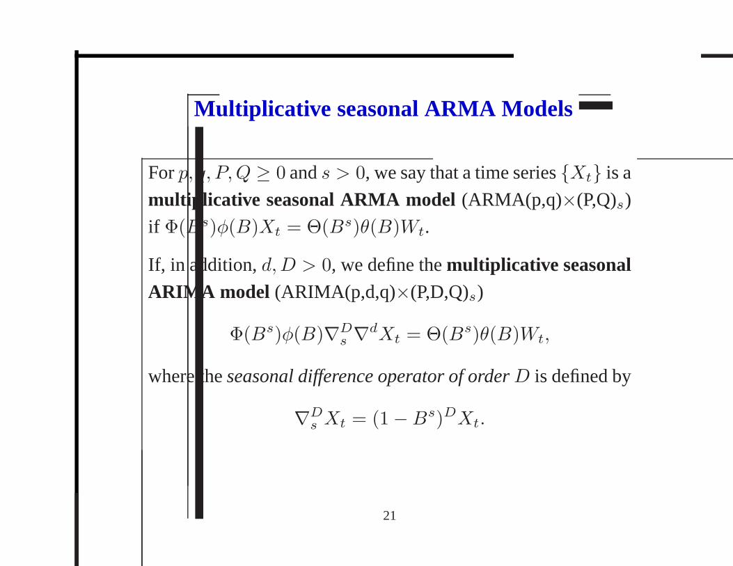
Multiplicative seasonal ARMA Models

Forp, q, P,Q ≥ 0 ands > 0, we say that a time series{Xt} is a

multiplicative seasonal ARMA model (ARMA(p,q)×(P,Q)s)

if Φ(Bs)φ(B)Xt = Θ(Bs)θ(B)Wt.

If, in addition,d,D > 0, we define themultiplicative seasonalARIMA model (ARIMA(p,d,q)×(P,D,Q)s)

Φ(Bs)φ(B)∇Ds ∇dXt = Θ(Bs)θ(B)Wt,

where theseasonal difference operator of order D is defined by

∇Ds Xt = (1−Bs)DXt.

21

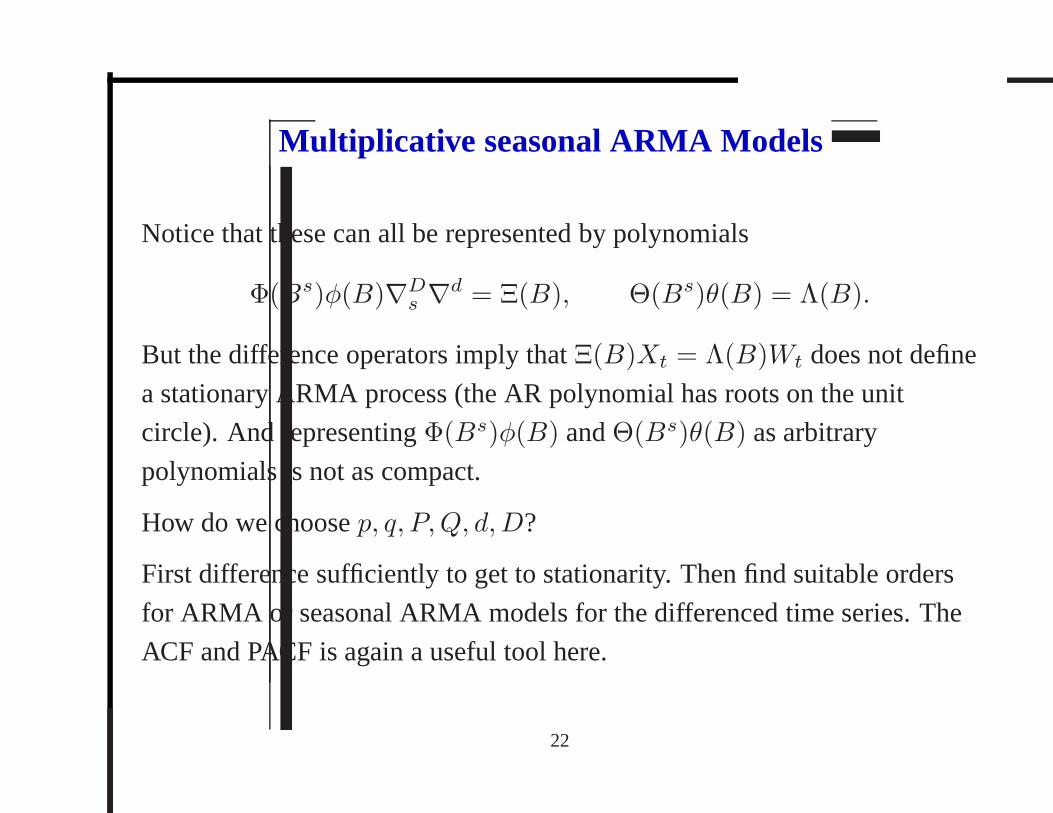
Multiplicative seasonal ARMA Models

Notice that these can all be represented by polynomials

Φ(Bs)φ(B)∇Ds ∇d = Ξ(B), Θ(Bs)θ(B) = Λ(B).

But the difference operators imply thatΞ(B)Xt = Λ(B)Wt does not define

a stationary ARMA process (the AR polynomial has roots on theunit

circle). And representingΦ(Bs)φ(B) andΘ(Bs)θ(B) as arbitrary

polynomials is not as compact.

How do we choosep, q, P,Q, d,D?

First difference sufficiently to get to stationarity. Then find suitable orders

for ARMA or seasonal ARMA models for the differenced time series. The

ACF and PACF is again a useful tool here.

22

Introduction to Time Series Analysis. Lecture 14.

1. Review: Maximum likelihood estimation

2. Computational simplifications: un/conditional least squares

3. Diagnostics

4. Model selection

5. Integrated ARMA models

6. Seasonal ARMA

7. Seasonal ARIMA models

23