Introduction to the field theory of classical and

quantum phase transitions

Flavio S. Nogueira

September 2010

Contents

1 Introduction 1

2 Ferromagnetism 4

2.1 Spin in an external magnetic field . . . . . . . . . . . . . . . . 4

2.2 The Landau-Lifshitz equation . . . . . . . . . . . . . . . . . . 8

2.3 The Berry vector potential, magnetic monopoles in spin space,

and hedgehogs in real space . . . . . . . . . . . . . . . . . . . 10

2.4 The classical nonlinear σ model . . . . . . . . . . . . . . . . . 12

2.4.1 The expansion in ε = d− 2 . . . . . . . . . . . . . . . . 13

2.4.2 The 1/n expansion . . . . . . . . . . . . . . . . . . . . 29

3 The Kosterlitz-Thouless phase transition 38

3.1 The XY model . . . . . . . . . . . . . . . . . . . . . . . . . . 38

3.2 Spin-wave theory . . . . . . . . . . . . . . . . . . . . . . . . . 39

3.3 Two-dimensional vortices . . . . . . . . . . . . . . . . . . . . . 42

3.4 The renormalization group for the Coulomb gas . . . . . . . . 47

4 Bose-Einstein condensation and superfluidity 55

4.1 Bose-Einstein condensation in an ideal gas . . . . . . . . . . . 55

i

4.2 The dilute Bose gas in the large N limit . . . . . . . . . . . . 60

4.2.1 The saddle-point approximation . . . . . . . . . . . . . 61

4.2.2 Gaussian fluctuations around the saddle-point approx-

imation: Bogoliubov theory and beyond . . . . . . . . 63

4.2.3 The excitation spectrum below Tc . . . . . . . . . . . . 68

4.2.4 Depletion of the condensate . . . . . . . . . . . . . . . 73

4.2.5 The superfluid density . . . . . . . . . . . . . . . . . . 76

5 Mott insulators 82

5.1 The Hubbard model . . . . . . . . . . . . . . . . . . . . . . . 82

5.2 The Bose-Hubbard model . . . . . . . . . . . . . . . . . . . . 90

5.3 The Heisenberg antiferromagnet . . . . . . . . . . . . . . . . . 105

5.3.1 Antiferromagnetic spin waves . . . . . . . . . . . . . . 105

5.3.2 The quantum O(n) non-linear σ model . . . . . . . . . 110

5.3.3 The CPN−1 model . . . . . . . . . . . . . . . . . . . . 112

5.3.4 Quantum electrodynamics in 2 + 1 dimensions . . . . . 127

Appendices 147

A The surface of a sphere in d dimensions 148

B Dimensional regularization and evaluation of some simple

integrals in d dimensions 150

C Evaluation of the integral over a Bose-Einstein distribution

in d dimensions 154

D Matsubara sums 157

ii

E Classical limit of the polarization bubble of the dilute Bose

gas 163

iii

Abstract

These lecture notes provide a relatively self-contained introduction to field

theoretic methods employed in the study of classical and quantum phase

transitions.

Chapter 1

Introduction

After the work of Wilson and others [1] in the 1970s on the renormalization

group (RG) in the theory of phase transitions, field theory methods originally

employed in high-energy physics became an indispensable tool in theoretical

condensed matter physics. Indeed, since the seminal work of Wilson, many

excellent textbooks on field theoretic methods in condensed matter physics

appeared, where a variety of other topics are also discussed; see, for exam-

ple, Refs. [2, 3, 4, 5, 6, 7, 8, 9, 10, 11, 12]. On the other side, the use of

field theoretic methods in condensed matter physics led to further insights

in particle physics. Thus, the study of classical phase transitions in several

lattice spin models gave birth to lattice gauge theory (for a review, see Ref.

[13]), which provided an approach to numerically tackle the strong-coupling

regime of gauge theories. This interchange of ideas between these two fields

became even more intensive after the discovery of high-temperature (high-

Tc) superconductors, where it became apparent that traditional many-body

techniques are insufficient to understand the mechanism behind high-Tc su-

1

perconductivity. For instance, gauge theories, both Abelian and non-Abelian

were employed to understand several properties of doped Mott insulators

[3, 7, 14], which eventually may become superconducting upon doping.

These notes have the aim of introducing some field theoretic methods

widely used in the study of classical and quantum phase transitions. Classi-

cal phase transitions occur at a regime where quantum fluctuations do not

play an important role, usually at high enough temperatures. In this case

time, as obtained from quantum-mechanical equations of motion, does not

play a role. Furthermore, in many situations is possible to use a continuum

model Hamiltonian, which provides the stage for employing the field theory

formalism. Wilson’s RG was originally introduced in this context [1]. The

Hamiltonians are in this case actually determined by a Landau-Ginzburg

type of expansion [15] where the free energy is expanded in powers of the

order parameter and its derivatives. The result is similar to Lagrangians of

quantum field theories in Euclidean space, i.e., a space-time where time is

imaginary [5]. It is this fact that allows for the application of field theory in

the study of phase transitions [2, 5, 8, 11]. Quantum phases transitions [6],

on the other hand, occur at zero temperature, such that time becomes impor-

tant. The quantum phase transition is usually driven by some dimensionless

parameter, like for example the ratio between two couplings appearing in a

quantum Hamiltonian. Very often the Lagrangian for a system undergoing

a quantum phase transition resembles one for a classical phase transition,

excepts that one of directions of space is the (imaginary) time. Thus, when

this occurs, the same field theoretic methods employed in the framework of

classical phase transitions can be applied in the quantum phase. Sometimes

2

we say in such a context that a quantum system in d + 1 spacetime dimen-

sions (i.e., d spatial dimensions and one time dimension) is equivalent to

a classical system having d + 1 spatial dimensions. Thus, if we think of a

Landau-Ginzburg theory, we see that the effective Lagrangian of the quantum

system has to look relativistic. There are several non-relativistic condensed

matter systems possessing an effective description which is relativistic-like

[3, 6, 7, 10, 11, 12]. Here “effective” means a field theory description valid

at some energy scale where the details of the underlying lattice model are

irrelevant. There are cases, however, where time arises in the effective theory

in a way which is not rotational invariant in d+1 spacetime dimensions 1. In

those situations, frequency scales differently from momenta near the critical

point, so they differ in scaling by some power [6, 9]. Thus, we can write the

scaling relation ω ∼ |p|z at the critical point, which defines the so called dy-

namic critical exponent, z. In this way, we see that a relativistic-like theory

will have z = 1, so that the results from classical phase transitions can be

applied to the quantum case more directly. We will see in these notes mostly

examples of theories having z = 1.

In these notes priority is given to the introduction of calculational meth-

ods. Thus, the reader will usually find here very detailed calculations, which

are often done step-by-step.

1When we say “rotational invariant” here, we are thinking of d+1 Euclidean dimensions.

3

Chapter 2

Ferromagnetism

2.1 Spin in an external magnetic field

Let us start with a very simple example spin dynamics, namely, the interac-

tion of a spin with an external magnetic field. The Hamiltonian is

H = −γS ·B. (2.1)

The Heisenberg equation of motion for the i-th spin component yields 1

i∂Si∂t

= [Si, H]

= −γ[Si, Sj]Bj. (2.2)

From the quantum mechanical commutation relation,

1From now on we assume that repeated indices are summed over.

4

[Si, Sj] = iεijkSk, (2.3)

we obtain immediately,

∂Si∂t

= −γεijkBjSk, (2.4)

or, in vector notation,

∂S

∂t= γ(S×B). (2.5)

The above equation simply describes the precession of a spin in an external

magnetic field.

The above equation can also be obtained from a Lagrangian for a classical

spin. The classical spin is given by S = Sn, where n2 = 1. In this case we

have the Lagrangian density,

L = S[A(n) · ∂tn + γn ·B], (2.6)

where the vector functional A(n) has to be determined. This functional plays

the role of a “momentum” canonically conjugate to n, so that A(n) · ∂tn

would play the role analogous to a term pdq/dt in classical mechanics. In

this context, we note that the Hamiltonian density H = −Sγn ·B does not

depend on A, which may appear to be a strange feature when compared to

the most common situations in classical mechanics. However, we should not

forget that we have a constraint, n2 = 1, which will play an important role

in the derivation of the equations of motion.

5

The equation of motion for each component of the unit vector field n is

given by the Euler-Lagrange equation:

∂t∂L

∂(∂tni)− ∂L∂ni

= 0. (2.7)

Thus, we have ∂L/[∂(∂tni)] = Ai(n), so that,

∂t∂L

∂(∂tni)= S

∂Ai∂nj

∂tnj. (2.8)

We also have,

∂L∂ni

= S

(∂Aj∂ni

∂tnj + γBi

). (2.9)

Altogether we obtain,

(∂Ai∂nj− ∂Aj∂ni

)∂tnj = γBi. (2.10)

The term between parentheses is an antisymmetric second-rank tensor which

is a function of the unit vector n. Therefore, it should have the form,

∂Ai∂nj− ∂Aj∂ni

= εijknk, (2.11)

or, equivalently,

εijk∂Ak∂nj

= ni. (2.12)

The LHS of Eq. (2.12) is the i-th component of the curl of A. We can

interpret A as a vector potential defined in spin space. It is actually called

6

the Berry vector potential, and the corresponding term in the Lagrangian

containing A, when associated to a functional integral representation of spin

systems [6], constitutes the so called Berry phase. We will study the Berry

vector potential further in a while. For the moment, let us proceed by deriv-

ing the equation of motion for n.

Using Eq. (2.12) in Eq. (2.10, we obtain easily,

εijknk∂tnj = γBi. (2.13)

Contracting both sides with εlminm yields,

εlmiεijknmnk∂tnj = γεlminmBi

=⇒ (δljδmk − δlmδjk)nmnk∂tnj = γεlminmBi

=⇒ ∂tnl = γ(n×B)l, (2.14)

where from the second line to the third we have used both n2 = 1 and

n · ∂tn = (1/2)∂tn2 = 0. Therefore, we have just obtained the desired result,

namely,

∂tn = γ(n×B) (2.15)

Thus, once more a precessing vector is obtained, except that this time it is

not an operator that is precessing.

7

2.2 The Landau-Lifshitz equation

Eq. (2.15) is the simplest example of the so called Landau-Lifshitz (LL)

equation. In order to study the dynamics of ferromagnetic systems, we have

to go beyond the situation of an external magnetic field. To do this, first

note that

Bi = − 1

S

δH

δni, (2.16)

where

H = −γS∫d3rn ·B. (2.17)

If H has a more complicate functional dependence on n, involving spatial

variations of the unit vector, B will be itself a function of n, constituting

in this way an effective magnetic field. By assuming spatial isotropy, such a

Hamiltonian is given by

H =

∫d3r

[JS2

2∂in · ∂in− γSn ·B

], (2.18)

where JS2, with J > 0, is the bare spin stiffness. The first term in the

Hamiltonian above can be motivated via the continuum limit of the lattice

spin Hamiltonian for a ferromagnet,

H = −J∑〈i,j〉

Si · Sj, (2.19)

8

where the lattice spin fields are assumed to be classical vectors, Si = Sni,

and the lattice sites are summed over nearest neighbors. Indeed, by inserting

the lattice Fourier transformation

Si =1√L

∑k

eik·RiSk, (2.20)

where L is the number of lattice sites, in the Hamiltonian above, we obtain,

H =∑k

J (k) Sk · S−k, (2.21)

where

J (k) = −2J3∑

α=1

cos kα, (2.22)

and we have set the lattice space equal to unity. In the continuum limit, we

have,

J (k) ≈ −6J +J

2k2. (2.23)

The second term above contributes to the first term in (2.18), while the term

−6J just adds an irrelevant constant to the Hamiltonian, since

−6J∑k

Sk · S−k = −6JS2∑i

n2i = −6JS2L. (2.24)

Let us consider now the LL equation with an effective field determined

by the Hamiltonian (2.18). The LL becomes,

9

∂tn = SJ(n×∇2n) + γ(n×B). (2.25)

Next we set B = 0 and study small transverse fluctuations around the

e3-axis, i.e.,

n =1√2e3 + δn⊥, (2.26)

where

δn⊥ =1√2

[cos(k · r− ωt)e1 + sin(k · r− ωt)e2]. (2.27)

This solution describes a so called spin-wave, whose quanta are known as

magnons. By inserting the above spin-wave profile in the LL equation, we

see that it solves it provided

ω =JS2

√2k2, (2.28)

which yields the spin-wave spectrum for a ferromagnet.

2.3 The Berry vector potential, magnetic monopoles

in spin space, and hedgehogs in real space

Let us discuss the Berry vector potential further. If we compute the flux of

the curl (in spin space) of A(n) through the unit sphere S2 (the bar reminds

us that S2 is embedded in spin space) using Eq. (2.12), we obtain,

10

∮S2

dSi εijk∂Ak∂nj

=

∮S2

dSi ni

=

∫ 2π

0

dξ

∫ π

0

dη

(∂n

∂ξ× ∂n

∂η

)· n

= 4πN, (2.29)

where we have used the parametrization n = (sin η cos ξ, sin η sin ξ, cos η),

and N ∈ Z is the winding number. This result shows that the Berry vector

potential corresponds to the field strength of a magnetic monopole in spin

space.

Note that this result is supposed to be an intrinsic property of the Berry

vector potential such that should hold beyond the case of a single spin in

an external field. However, for the case where many spins are involved and

have a gradient energy, we have a further topological aspect. In fact, when

n has a nonzero gradient, we have the following flux through a sphere S2

in real space (note the absence of the bar over S2 and the differences in the

integration measure),

∮S2

dSiεijkn · (∂jn× ∂kn) =

∫ 2π

0

dϕ

∫ π

0

dθεilm∂xl∂ϕ

∂xm∂θ

εijkn · (∂jn× ∂kn)

=

∫ 2π

0

dϕ

∫ π

0

dθ(δljδmk − δlmδjk)∂xl∂ϕ

∂xm∂θ

n · (∂jn× ∂kn)

= 2

∫ 2π

0

dϕ

∫ π

0

dθn ·(∂xl∂ϕ

∂n

∂xl× ∂xm

∂θ

∂n

∂xm

)= 2

∫ 2π

0

dϕ

∫ π

0

dθn ·(∂n

∂ϕ× ∂n

∂θ

). (2.30)

11

We see that the last line of (2.30) is twice the second line of (2.29). Thus,

we have,

1

2

∮S2

dSiεijkn · (∂jn× ∂kn) = 4πN. (2.31)

Therefore, we see that there is not only a topological object living in spin

space, but there is also one living in real (three-dimensional) space, a so called

hedgehog. Just like the magnetic monopole in spin space, the hedgehog in real

space is also a point-like topological object. These topological objects arise

also in two-dimensional quantum antiferromagnets, which will be discussed

later in these notes.

2.4 The classical nonlinear σ model

In order to study the static critical behavior of a ferromagnet, we can consider

just the Hamiltonian (2.18) and try to compute the partition function via

the functional integral representation,

Z =

∫Dnδ(n2 − 1)e−

1T

Rd3rH, (2.32)

where the δ function enforces the constraint. We can rescale the coordinates

and the temperature such as to have only 1/T as the coefficient of the gradient

termH and remove the prefactor JS2. We will also generalize the model such

that it will have d dimensions and the unit vector field will have n components

instead of three. In this way, we will be able to consider two approximation

schemes, namely, one where an expansion in ε = d− 2 is made, and another

12

one where the number of components n is large, such that an expansion in

1/n can be done.

2.4.1 The expansion in ε = d− 2

The main idea behind all ε-expansions is to make a perturbative analysis

of the problem around the dimensionality where the coupling constant of

the model is dimensionless. In such a case, at the so called critical dimen-

sion (i.e., the dimension that makes the coupling constant dimensionless),

perturbation theory is relatively well behaved. The perturbation series is

still divergent and frequently needs to be resummed, especially when higher

orders in perturbation theory is involved. However, rigorous mathematical

results exist in some cases where out of some (initially) perturbation series a

non-perturbative expansion may be rigorously constructed [16]. The situa-

tion is considerably more difficult if we are not at the critical dimension and

the theory approaches the critical point, thus becoming strongly coupled. In

these cases there are several resummation procedures; for a review on these,

with focus on variational perturbation theory, see the textbook by Kleinert

and Schulte-Frohlinde [8].

For the classical non-linear σ model, the coupling constant is the tem-

perature T . Simple dimensional analysis shows that this coupling becomes

dimensionless at d = 2. We will show later that for d = 2 the model is

actually asymptotically free. We are ultimately interested at d = 3, so the

goal will be to set ε = 1 at the end of the calculations. The case d = 2 and

n = 2 is special and will be treated separately in the next chapter.

13

The calculations will be performed up to second order in the temperature

and will serve as a good introduction to the calculation of loop integrals

occurring in Feynman diagrams. Therefore, we will perform all integrals

exactly in d dimensions and in great detail below. Simple properties of

analytical continuation of the dimension in the integrals will be assumed.

This is known as dimensional regularization. The properties of dimensional

regularization are very simple and are discussed in several textbooks; see for

example Ref. [8]

By resolving the constraint n2 = σ2 + π2 = 1, the Hamiltonian of the

nonlinear σ model can be written as

H =1

2T

[(∂iπ)2 +

(∂i√

1− π2)2]

=1

2T

[(∂iπ)2 +

(π · ∂iπ)2

1− π2

], (2.33)

where π = (π1, . . . , πn−1).

The Green function can be written as [n = (σ,π)]

G(x) = 〈n(x) · n(0)〉

= 〈σ(x)σ(0)〉+ 〈π(x) · π(0)〉

= 〈√

1− π2(x)√

1− π2(0)〉+ 〈π(x) · π(0)〉. (2.34)

If one rescales π by√T and expand up to order T , we obtain

14

G(x) = 1− T

2〈π2(x) + π2(0)〉+ T 〈π(x) · π(0)〉+O(T 2)

= 1 + (n− 1)T [G0(x)−G0(0)] +O(T 2), (2.35)

where

G0(x) =

∫p

eip·x

p2, (2.36)

and we have used the short-hand notation

∫p

≡∫

ddp

(2π)d. (2.37)

Note that we have used translation invariance to write 〈π2(x)〉 = 〈π2(0)〉 =

(n− 1)G0(0).

The dimensional regularization rules demand that (see, for example, the

textbook [8] and Appendix B)

∫q

1

|q|α= 0, for all α, (2.38)

which immediately leads to G0(0) = 0.

In order to calculate G0(x) explicitly we use Feynman parameters:

G0(x) =

∫ ∞0

dλ

∫p

eip·x−λp2

(2.39)

By performing the Gaussian integral in p (by just completing the squares),

we obtain

15

G0(x) =1

(4π)d/2

∫ ∞0

dλλ−d/2 exp

(−x

2

4λ

). (2.40)

The substitution u = x2/(4λ) yields

G0(x) =2d−2

(4π)d/2|x|d−2

∫ ∞0

duu(d−2)/2−1e−u

=2d−2Γ(d/2− 1)

(4π)d/2|x|d−2=

1

(d− 2)Sd|x|d−2, (2.41)

where Sd = 2πd/2/Γ(d/2) is the surface of the unit sphere in d dimensions

(see Appendix A) and we have made use of the definition of the gamma

function:

Γ(z) =

∫ ∞0

dττ z−1e−τ . (2.42)

By performing the substitution τ = as, with a constant, the above definition

of the gamma function gives another very useful formula in calculations with

dimensional regularization:

1

az=

1

Γ(z)

∫ ∞0

dssz−1e−as. (2.43)

To illustrate the usefulness of this formula, let us calculate two functions that

will be needed later:

Gα(x) =

∫p

eip·x

(p2)α/2(2.44)

and

16

Iα(p) =

∫q

1

q2[(p+ q)2]α/2, (2.45)

where α ∈ R.

Using Eq. (2.43), we obtain for Eq. (2.44),

Gα(x) =1

Γ(α/2)

∫ ∞0

dτ

∫p

τα/2−1e−τp2+ip·x

=1

(4π)d/2Γ(α/2)

∫ ∞0

dττ (α−d)/2−1 exp

(−x

2

4τ

)=

2d−α

(4π)d/2Γ(α/2)|x|d−α

∫ ∞0

duu(d−α)/2−1e−u

=2d−αΓ

(d−α

2

)(4π)d/2Γ(α/2)|x|d−α

. (2.46)

Note that by setting α = 2 we recover the expression for G0(x).

The calculation of Iα(p) is more involved. By using Eq. (2.43), we can

write

Iα(p) =1

Γ(α/2)

∫ ∞0

dτ1

∫ ∞0

dτ2

∫ddq

(2π)dτα/2−12 e−p

2τ2−q2(τ1+τ2)−2p·qτ2 . (2.47)

After performing the Gaussian integral in q, we obtain

Iα(p) =1

(4π)d/2Γ(α/2)

∫ ∞0

dτ1

∫ ∞0

dτ2τα/2−12

(τ1 + τ2)d/2exp

(− p

2τ1τ2

τ1 + τ2

). (2.48)

Now we perform the change of variables

17

τ1 = τσ, τ2 = (1− τ)σ, (2.49)

where 0 ≤ τ ≤ 1 and 0 ≤ σ <∞. Note that the Jacobian of the transforma-

tion is σ. The result is

Iα(p) =1

(4π)d/2Γ(α/2)

∫ 1

0

dτ

∫ ∞0

dσe−p

2τ(1−τ)σ

σ(d−α)/2(1− τ)1−α/2 . (2.50)

After introducing the change of variables s = p2τ(1− τ)σ, the above integral

can be rewritten as

Iα(p) =|p|d−α−2

(4π)d/2Γ(α/2)

∫ 1

0

dττ (d−α−2)/2

(1− τ)(4−d)/2

∫ ∞0

dse−ss(α−d)/2

=|p|d−α−2

(4π)d/2Γ(α/2)Γ

(2 + α− d

2

)∫ 1

0

dττ (d−α−2)/2(1− τ)(d−4)/2

=|p|d−α−2

(4π)d/2Γ(α/2)Γ

(2 + α− d

2

)Γ

(d− 2

2

)Γ(d−α

2

)Γ(d− 1− α/2)

,(2.51)

where from the second line to third we have used the integral

∫ 1

0

dxxa(1− x)b =Γ(1 + a)Γ(1 + b)

Γ(2 + a+ b). (2.52)

We can easily go up to third order in T using the methods illustrated in

the paper of Amit and Kotliar [17]. Up to second order in T , for example,

we can proceed as before and expand further√

1− Tπ2(x) to obtain

18

〈√

1− Tπ2(x)√

1− Tπ2(0)〉 = 1− (n− 1)TG0(0)− T 2

4〈π2(x)π2(0)〉+ . . .

= 1− T 2

4〈π2(x)π2(0)〉+ . . . , (2.53)

where we have used dimensional regularization to setG0(0) = 0. The remaing

avarage involving four pi fields can be decoupled with the help of Wick’s

theorem, i.e.,

〈π2(x)π2(0)〉 = 2[〈π(x) · π(0)〉 − 〈π2(x)〉〈π2(0)〉]

= 2(n− 1)[G20(x)−G2

0(0)] = 2(n− 1)G20(x). (2.54)

The third order contribution is more difficult to obtain, since in this case

the non-linear factor

exp

[−1

2

∫ddx

(π · ∂iπ)2

1− Tπ2

](2.55)

in the partition function has to be taken into account when performing the

correlation function average. By expanding the exponential factor above in

powers of T we obtain also derivative contributions. The latter are more

easily handled with in momentum space. Afterwards we can transform the

result to real space. Thus, we have the following expansion,

19

G(p) = (2π)dδd(p) + T (n− 1)/p2 +1

2T 2(n− 1)Ib(p)

+ T 3(n− 1)

[1

2(n− 1)Ic(p) + Id(p)−

1

4(n− 1)Ie(p)−

1

2If (p)

],

(2.56)

where [17]

Ib(p) =

∫q

1

q2(p+ q)2, (2.57)

Ic(p) =1

p4

∫q

∫q1

(p+ q)4

q2q21(p+ q + q1)2

, (2.58)

Id(p) =1

p4

∫q

∫q1

(p+ q)2(p+ q1)2

q2q21(p+ q + q1)2

, (2.59)

Ie(p) = p2I2b (p), (2.60)

and

If (p) =

∫q

∫q1

(q − q1)2

q2(p+ q)2q21(p+ q1)2

. (2.61)

Note that the integral Ib appearing in the term of second order in T is

just the Fourier transform of Eq. (2.54), taking into account also Eq. (2.53).

However, it is instructive as one more exercise in dimensional regularization

to perform the integral Ib. This can be done straightforwardly by considering

20

Eq. (2.51) with α = 2 to obtain

Ib(p) = c(d)|p|d−4, (2.62)

where

c(d) =Γ(2− d/2)Γ2(d/2− 1)

(4π)d/2Γ(d− 2). (2.63)

Using Eq. (2.46), we obtain

Ib(x) = G20(x), (2.64)

which corresponds to the expected result, in view of Eqs. (2.53) and (2.54).

Integrating over q1 in Ic, using the result of Ib, we obtain

Ic(p) =c(d)

p4

∫q

1

q2[(p+ q)2]−d/2. (2.65)

By using Eq. (2.51) with α = −d, we obtain

Ic(p) =c(d)Γ(1− d)Γ(d/2− 1)Γ(d)

(4π)d/2Γ(−d/2)Γ(3d/2− 1)|p|2(d−3). (2.66)

Next we can use Eq. (2.46) to obtain Ic(x):

Ic(x) =d

9d− 12G3

0(x). (2.67)

The integral Id(p) can be written in the form

21

Id(p) = Jd(p)/p2 +Kd(p)/p

4 + p−4

∫q

∫q1

(p+ q)2

q2(p+ q + q1)2, (2.68)

Jd =

∫q

∫q1

(p+ q)2

q2q21(p+ q + q1)2

, (2.69)

and

Kd =

∫q

∫q1

2p · q1(p+ q)2

q2q21(p+ q + q1)2

. (2.70)

The last integral in Eq. (2.68) vanishes due to the rule (2.38) (by integrating

over q1).

Using (2.51) with α = 2 to integrate over q1, we obtain

Jd = c(d)

∫q

1

q2[(p+ q)2](2−d)/2(2.71)

Now we use once more (2.51), but this time with α = 2− d, to obtain

Jd(p) ≡ Jd(p)/p2 =

Γ(2− d/2)Γ3(d/2− 1)Γ(d− 2)Γ(d− 1)

(4π)dΓ(d− 2)Γ(1− d/2)Γ(3d/2− 2)|p|2(d−3). (2.72)

For Kd we need first to calculate

(p+ q)µI =

∫q1

q1µ

q21(p+ q + q1)2

, (2.73)

i.e.,

22

I =1

(p+ q)2

∫q1

q1 · (p+ q)

q21(p+ q + q1)2

=1

2(p+ q)2

∫q1

(p+ q + q1)2 − (p+ q)2 − q21

q21(p+ q + q1)2

= −1

2

∫q1

1

q21(p+ q + q1)2

= −c(d)

2[(p+ q)2](d−4)/2, (2.74)

where rule (2.38) has been used in the first and last terms of the second line

of the above equation. Using this result in the expression for Kd, we obtain

Kd(p) = −c(d)

∫q

p · (p+ q)

q2[(p+ q)2](2−d)/2

= −p2Jd − c(d)Ld(p), (2.75)

where

Ld(p) =

∫q

p · qq2[(p+ q)2](2−d)/2

=1

2

∫q

(p+ q)2 − p2 − q2

q2[(p+ q)2](2−d)/2

=p4Ic(p)

2c(d)− p2Jd(p)

2c(d). (2.76)

At the end, we obtain

23

Id(x) =1

2[Jd(x)− Ic(x)]

=1

3

d− 2

3d− 4G3

0(x). (2.77)

Since Ie(p) = p2I2b (p), we have

Ie(x) = c2(d)

∫p

eip·x

|p|2(3−d), (2.78)

which can be solved using (2.46) with α = 2(3− d). We have,

Ie(x) =c2(d)23(d−2)Γ(3d/2− 3)

(4π)d/2Γ(3− d)|x|3(d−2). (2.79)

For If (p), it is easy to see by expanding (q − q1)2 that

If (p) = 2

∫q

∫q1

1

q2(p+ q)2(p+ q1)2− 2

∫q

∫q1

q · q1

q2(p+ q)2q21(p+ q1)2

. (2.80)

The first integral above vanishes because of (2.38), and we obtain

If (p) = −2

[∫q

qµq2(p+ q)2

]2

. (2.81)

We can now use (2.74) with p+ q replaced by p to obtain

If (p) = −c2(d)

2|p|2(d−3). (2.82)

Therefore,

24

If (x) = − c2(d)23(d−2)Γ(3d/2− 3)

2(4π)d/2Γ(3− d)|x|3(d−2). (2.83)

In the expression for G(x) it is the following combination that appears:

1

4(n− 1)Ie(x) +

1

2If (x) = −(n− 2)

2

cos(πd/2)Γ(2− d/2)Γ(3d/2− 3)

Γ(d− 2)G3

0(x).

(2.84)

Therefore,

G(x) = 1 + T (n− 1)G0(x) +T 2

2(n− 1)G2

0(x)

+ (n− 1)T 3G30(x)

[(n+ 1)d− 4

6(3d− 4)+

(n− 2) cos(πd/2)Γ(2− d/2)Γ(3d/2− 3)

2Γ(d− 2)

]+ O(T 4). (2.85)

The above is the final expression for G(x) up to third order in T . By

setting d = 2 + ε and expanding for small ε, we obtain exactly the same

expression as in the paper of Amit and Kotliar [17], i.e.,

G(x) = 1 + T (n− 1)G0(x) +T 2

2(n− 1)G2

0(x)

+ T 3(n− 1)

{−n− 3

6− (n− 2)ε

6

+(n− 2)ε2

4+ε3

4(n− 2)

[ζ(3)− 3

2

]}, (2.86)

Note that due to the expression for G0(x), Eq. (2.86) contains poles for ε = 0.

25

These poles can be subtracted by introducing two renormalization constants

[18, 17], Z and Zt, such that the renormalized correlation function reads

Gr(x; t) = Z−1G(x;T = Ztµ−εt), (2.87)

having no poles for ε = 0.

The bare correlation function should be independent of the renormaliza-

tion scale µ, which is expressed by the equation,

µdG

dµ= µ

d

dµ[ZGr(x, t)] = 0, (2.88)

or, using the chain rule,

[µ∂

∂µ+ β(t)

∂

∂t+ ζ(t)

]G(x;T = Ztµ

−εt) = 0, (2.89)

where the renormalization group (RG) functions β(t) and ζ(t) are given by

β(t) ≡ µ∂t

∂µ, ζ(t) ≡ µ

∂ lnZ

∂µ. (2.90)

Using the derived perturbative expansion for the correlation function, we

obtain,

β(t) = εt− (n− 2)t2 − (n− 2)t3, (2.91)

ζ(t) = (n− 1)t+3

4(n− 1)(n− 2)t3. (2.92)

The vanishing of the β function determines the critical temperature as an

26

expansion in powers of ε,

tc =ε

n− 2

[1− ε

n− 2+ε2

4

(6− nn− 2

)]+O(ε4). (2.93)

In terms of the RG functions above, the exponents ν and η are respectively

given by [17]

ν = − 1

β′(tc), η = ζ(tc)− ε, (2.94)

corresponding to the critical behavior

ξ ∼ (t− tc)−ν , (2.95)

where ξ is the correlation length, and

G(x) ∼ 1

|x|d−2+η. (2.96)

The correspondence between the RG functions and the critical exponents

follows by making dimensionless variables in G(x) explicit. For instance, we

can write,

G(x) ∼(µ

Λ

)ε+η(µ|x|)−ε−η, (2.97)

where Λ is the ultraviolet cutoff. Thus, we have the behavior,

Z ∼(µ

Λ

)−(ε+η)

. (2.98)

Therefore, near the critical point we have,

27

µ∂ lnZ

∂µ≈ −ε− η. (2.99)

Comparison with Eq. (2.92) yields the second of Eqs. (2.94).

For the critical exponent ν, we linearize the β function near the critical

point tc, i.e.,

µ∂(t− tc)∂µ

≈ −β′(tc)(t− tc), (2.100)

where the prime denote a derivative with respect to t and the minus sign

reflects the negative slope of the β function at tc (ultraviolet stability of the

fixed point). Integrating the above equation yields

µ

Λ∼ (t− tc)−1/β′(tc), (2.101)

which upon the identification µ = ξ−1 leads to the determination of the

critical exponent ν.

Explicitly, we have

1

ν= ε+

ε2

n− 2+O(ε3), (2.102)

η =ε

n− 2

[1−

(n− 1

n− 2

)ε+

n(n− 1)

2(n− 2)2ε2]

+O(ε4). (2.103)

Note that the calculations allow to obtain η with one order of ε higher than

for 1/ν.

28

2.4.2 The 1/n expansion

The saddle-point approximation

A common nonperturbative approach to study the non-linear σ is the large

n limit [6, 5], where n is taken to be large while ng is kept fixed. Such an

analysis is more easily done if the constraint is implemented with the help of

a Lagrange multiplier field, such that the Lagrangian becomes

L =1

2g[(∂in)2 + iλ(n2 − 1)]. (2.104)

This Lagrange multiplier field arises from the partition function (2.32) when

the functional integral representation of the delta function is used:

δ(n2 − 1) =

∫Dλe−

12T

Rddxiλ(n2−1). (2.105)

Let us integrate n−1 components of n exactly and call the non-integrated

one σ. The resulting effective action reads

Seff =(n− 1)

2Tr ln(−∇2 + iλ) +

1

2T

∫ddx[σ(−∇2 + iλ)σ − iλ]. (2.106)

The limit n → ∞ is obtained from the saddle-point approximation to the

above effective action. We will consider a uniform saddle-point with iλ = m2

and σ = s. Thus, from

∂Seff

∂m2= 0,

∂Seff

∂s= 0, (2.107)

29

we obtain,

s2 = 1− nT∫

ddp

(2π)d1

p2 +m2, (2.108)

m2s = 0. (2.109)

For T < Tc we have s 6= 0, so that m2 = 0, leading to

s2 = 1− nT∫

ddp

(2π)d1

p2. (2.110)

At the critical point, T = Tc, we have that s = 0, so that

1

nTc=

∫ddp

(2π)d1

p2=

SdΛd−2

(2π)d(d− 2), (2.111)

where Λ is the ultraviolet cutoff. Therefore,

s2 =1

Tc(Tc − T ), (2.112)

which implies that the critical exponent of the order parameter is β = 1/2.

For T > Tc, on the other hand, we have s = 0 and m2 6= 0, such that

∫ddp

(2π)d1

p2 +m2=

1

nT. (2.113)

If we now write

1 = nT

(∫ddp

(2π)d1

p2 +m2−∫

ddp

(2π)d1

p2+

∫ddp

(2π)d1

p2

), (2.114)

30

we obtain,

T − TcTc

= nTm2

∫ddp

(2π)d1

p2(p2 +m2). (2.115)

The integral above can be evaluated with help of the integral I1 of Appendix

B. Indeed, it is proportional to the integral I1 evaluated in d−2 dimensions,

i.e.,

∫ddp

(2π)d1

p2(p2 +m2)=

1

2π(d− 2)I1(d− 2) =

21−dπ−d/2md−4

d− 2Γ

(2− d

2

).

(2.116)

Thus,

21−dπ−d/2

d− 2Γ

(2− d

2

)nTmd−2 =

T − TcTc

, (2.117)

or, after substituting the value of Tc, Eq. (2.111),

m = Λ

{πd/2−2

Γ(d/2)Γ(2− d/2)

[1− (2π)d(d− 2)Λ2−d

SdnT

]}1/(d−2)

(2.118)

It turns out that the mass gap m = ξ−1, where ξ is the correlation length.

Therefore, the corresponding critical exponent is

ν =1

d− 2. (2.119)

The limit d→ 2 of Eq. (2.118) yields 2

2We are making use of the well-known result ex = limm→∞(1 + x/m)m.

31

m =Λ

πexp

(− 2π

nT

), (2.120)

which implies that for d = 2 the system is gapped for all T > 0, i.e., no

phase transition occurs in this case. This is consistent with the Mermin-

Wagner theorem [20], which states that a continuous symmetry associated

to quadratic dispersions cannot be broken in d = 2. Note that the Mermin-

Wagner theorem rules out the symmetry breaking at d = 2, but not neces-

sarily the phase transition. Indeed, we will see in the next chapter that d = 2

and n = 2 is special. In fact, although no symmetry breaking occurs in this

case, a phase transition happens even in its absence.

The β function for the dimensionless coupling t = Λd−2T at large n is

easily obtained by demanding the scale invariance of the mass gap, i.e.,

Λ∂m

∂Λ= 0, (2.121)

which yields,

Λ∂t

∂Λ= (d− 2)t− Sd

(2π)dnt2, (2.122)

and we see that for d = 2 the theory is asymptotically free.

1/n corrections to the saddle-point

Now we want to compute the 1/n corrections to the saddle-point calculation.

Let us consider for instance the theory at the critical temperature and find

the anomalous dimension of the σ-field. This is achieved by first expanding

32

the effective action (2.106) up to quadratic order in λ, such as to obtain the

λ-propagator. This yields

Seff ≈n

4

∫ddx

∫ddx′G0(x−x′)G0(x′−x)λ(x)λ(x′)+

1

2T

∫ddxσ(−∇2+iλ)σ,

(2.123)

where G0(x) is given in Eq. (2.36). Thus, it is easy to obtain the correlation

function for the field λ in momentum space as

〈λ(p)λ(−p)〉 =(2/n)∫

ddq(2π)d

1q2(p+q)2

, (2.124)

or, using the result (2.62),

〈λ(p)λ(−p)〉 =2

c(d)n|p|d−4, (2.125)

where c(d) is given in Eq. (2.63). In order to find the anomalous dimension

of the σ-field we need to compute the σ-propagator up to order 1/n. This

is done by taking into account the vertex iλσ2/(2T ) in Eq. (2.123). The

lowest order contribution to the σ-propagator features two vertices. The

corresponding Feynman diagram is shown in Fig. 2.1. Thus,

〈σ(p)σ(−p)〉−1 = p2 +

∫ddq

(2π)d〈λ(p+ q)λ(−p− q)〉

q2

= p2 +2

nc(d)

∫ddq

(2π)d1

|p+ q|d−4q2. (2.126)

33

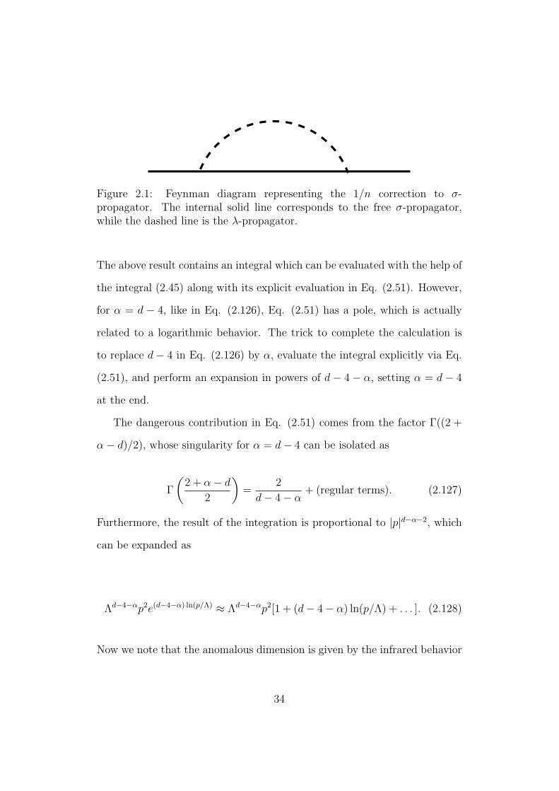
Figure 2.1: Feynman diagram representing the 1/n correction to σ-propagator. The internal solid line corresponds to the free σ-propagator,while the dashed line is the λ-propagator.

The above result contains an integral which can be evaluated with the help of

the integral (2.45) along with its explicit evaluation in Eq. (2.51). However,

for α = d − 4, like in Eq. (2.126), Eq. (2.51) has a pole, which is actually

related to a logarithmic behavior. The trick to complete the calculation is

to replace d− 4 in Eq. (2.126) by α, evaluate the integral explicitly via Eq.

(2.51), and perform an expansion in powers of d − 4 − α, setting α = d − 4

at the end.

The dangerous contribution in Eq. (2.51) comes from the factor Γ((2 +

α− d)/2), whose singularity for α = d− 4 can be isolated as

Γ

(2 + α− d

2

)=

2

d− 4− α+ (regular terms). (2.127)

Furthermore, the result of the integration is proportional to |p|d−α−2, which

can be expanded as

Λd−4−αp2e(d−4−α) ln(p/Λ) ≈ Λd−4−αp2[1 + (d− 4− α) ln(p/Λ) + . . . ]. (2.128)

Now we note that the anomalous dimension is given by the infrared behavior

34

of the propagator, i.e.,

〈σ(p)σ(−p)〉 ∼ 1

p2−η . (2.129)

Thus, before setting α = d − 4, we neglect the terms which are smalller in

comparison with p2−η as p → 0, anticipating already that η > 0. Thus, by

keeping only the dominant terms in the infrared, we can safely set α = d− 4

to obtain

〈σ(p)σ(−p)〉−1 ≈ p2

[1 +

2(d− 4)Γ(d− 2)

nΓ(2− d/2)Γ(d/2 + 1)Γ2(d/2− 1)ln( p

Λ

)],

(2.130)

which should be compared to

p2−η ≈ p2[1− η ln(p/Λ)], (2.131)

to obtain, after some simplifications,

η =(4− d)(d− 2)2Γ(d− 2)

ndΓ(2− d/2)Γ3(d/2). (2.132)

For d = 3 this yields

η =8

3π2n. (2.133)

The above result for η is the same as obtained for the O(n) Landau-Ginzburg

model at large n. Indeed, both models have in the framework of a 1/n

expansion the same critical exponents, belonging henceforth to the same

35

universality class [5].

In order to see the non-perturbative character of Eq. (2.132), let us

compare this expression with the perturbative expansion in powers of ε =

d− 2 in Eq. (2.103) for n large. If we expand Eq. (2.132) in powers of ε, we

obtain

η =ε

n

(1− ε+

ε2

2+ . . .

), (2.134)

which is precisely Eq. (2.103) in the limit n � 1. The large n result agrees

with the large n regime of the ε-expansion even up to order four. Indeed,

we have that up to this order the anomalous dimension is given by (see for

example Ref. [5] and references therein)

η = ε+ (n− 1)ε2{−1 +

n

2ε

+

[−b+ (n− 2)

(2− n

3+

3− n4

ζ(3)

)]ε2}

+O(ε5), (2.135)

where we have defined

ε =ε

n− 2, (2.136)

and

b = − 1

12(n2 − 22n+ 34) +

3

2ζ(3)(n− 3). (2.137)

In the limit n� 1 Eq. (2.135) becomes

36

η =ε

n

(1− ε+

ε2

2− 1 + ζ(3)

4ε3)

+O(ε5), (2.138)

which agrees precisely with the expansion of Eq. (2.132) in powers of ε up

to the same order. This comparison clearly exhibits the non-perturbative

character of the 1/n expansion, since the lowest non-trivial 1/n correction to

η is already able to reproduce the large n limit of perturbation theory up to

fourth order.

37

Chapter 3

The Kosterlitz-Thouless phase

transition

3.1 The XY model

When n = 2, the local constraint n2i = 1 in the classical Heisenberg model is

solved by writing

ni = (cos θi, sin θi), (3.1)

such that the Heisenberg Hamiltonian becomes

H = −JS2∑〈i,j〉

cos(θi − θj). (3.2)

Such a planar magnetic system is known as XY model. As we will see in a

later Chapter, this model is in the same universality class as a superfluid.

The reason is not difficult to understand, since universality classes are usually

38

determined by the underlying symmetry group, which in the present case

is O(2), and this is the same as the unitary group U(1). The spontaneous

symmetry breaking of the U(1) group will be studied in several ways for d > 2

in the next Chapters. Here we will explore the case n = 2 and d = 2, where

no spontaneous symmetry breaking occurs, as we have already mentioned in

the last Chapter. While for n > 2 no phase transition can occur at d = 2,

the situation is different for n = 2. When n = 2 and d = 2 a phase transition

occurs without spontaneous symmetry breaking.

3.2 Spin-wave theory

Let us consider the classical non-linear σ model for n = 2. By writing

n = (cos θ, sin θ), we obtain,

H =1

2T(∇θ)2. (3.3)

The above equation is just the continuum limit of the XY model in Eq. (3.2),

up to a trivial renaming of the couplings.

It is easy to see that the correlation function G(x) = 〈n(x) · n(0)〉 of the

non-linear σ model can be written in this case as 1

G(x) = 〈ei[θ(x)−θ(0)]〉. (3.4)

More explicitly,

1Note that translation invariance implies 〈cos θ(x) sin θ(0)〉 = 〈sin θ(x) cos θ(0)〉.

39

G(x) =1

Z

∫Dθe−

Rddx′[ 1

2T(∇′θ)2−J(x′)θ(x′)], (3.5)

where Z is the partition function and

J(x′) = i[δd(x− x′)− δd(x′)]. (3.6)

Note that we are not setting d = 2 yet. We will see soon why it is convenient

to do so. We can perform the Gaussian integral over θ exactly to obtain

G(x) = exp

[T

2

∫ddx′

∫ddx′′J(x′)G(x′ − x′′)J(x′′)

]= exp {T [G(x)− G(0)]} , (3.7)

where

G(x) =

∫ddp

(2π)deip·x

p2. (3.8)

We are not going to use dimensional regularization in this Chapter. It is

actually essential to us not to have G(0) = 0. This is important, in order

to take the limit d → 2 in a clean way. Thus, by evaluating G(0) explicitly

using a cutoff, we obtain,

G(0) =SdΛ

d−2

(2π)d(d− 2). (3.9)

From Eq. (2.41), we obtain

40

G(x) =|x|2−d

Sd(d− 2). (3.10)

Thus,

G(x)− G(0) =SdΛ

d−2

(2π)d(d− 2)

[(2π)d

S2d

(Λ|x|)2−d − 1

], (3.11)

which has a straightforward limit d→ 2,

G(x)− G(0) = − 1

2πln(Λ|x|). (3.12)

Therefore, we have

G(x) =1

(Λ|x|)η(T ), (3.13)

where

η(T ) =T

2π, (3.14)

is the anomalous dimension of the theory. Interestingly, in contrast with

the case d > 2, the correlation function for n = 2 and d = 2 features a

temperature-dependent anomalous dimension. This is a particularity of the

two-dimensional XY model, as shown first by Kosterlitz and Thouless [21].

The above result is exact within spin-wave theory, which corresponds to

a situation where the fact that θ is an angle is not taken into account. The

periodicity of θ is, however, crucial for characterizing the phase structure of

the model. This will be the subject of the next Section.

41

Before closing this Section, let us point out the agreement between the

perturbation theory for the non-linear σ model for n = 2 and the results of

this Section. Indeed, if we set n = 2 in Eq. (2.85), we obtain,

G(x) = 1 + TG0(x) +T 2

2G0(x) +

T 3

6G3

0(x) +O(T 4). (3.15)

The above expansion contains the first terms of the expansion of exp[TG0(x)].

Note that G0(x) is the same as G(x) in this Section. Furthermore, since we

are not using dimensional regularization, we must make the replacement

G0(x)→ G(x)− G(0).

Another point worth mentioning in the context of the perturbation theory

of the previous chapter is that for n = 2 and d = 2 the β function (2.91)

vanishes, i.e.,

µ∂t

∂µ= 0. (3.16)

Thus, for n = 2 and d = 2 perturbation theory is just reproducing the result

of spin-wave theory, i.e., a free theory.

3.3 Two-dimensional vortices

We have already mentioned in the previous Section that the spin-wave theory

neglects the periodicity of θ. Thus, the spin-wave analysis implies

∮C

dx · ∇θ = 0. (3.17)

42

The above is not always true in the case of a periodic field [21, 2, 22]. This

is precisely the case if we interpret ∇θ as the superfluid velocity 2. In the

presence of vortices, the circulation of the superfluid velocity is quantized,

∮C

dx · ∇θ = 2πn, (3.18)

where n ∈ Z is the winding the number counting how many times the

closed curve C goes around the vortex. The equation above is just the

Bohr-Sommerfeld quantization condition applied to a superfluid.

In two dimensions vortices are just points. Thus, the problem of studying

the statistical mechanics of many vortices in two dimensions is much easier

as in three dimensions. In three dimensions vortices are either infinite lines

or loops. The statitiscal mechanics of vortex loops is much more complicated

and requires often the use of special duality techniques involving multivalued

fields [2, 22].

Let us give a concrete example of a single vortex at the origin in two

dimensions. Such a vortex has to be singular at x = (x1, x2) = (0, 0). Such

a vortex configuration is simply given by

∇θ =1

x2(−x2, x1). (3.19)

Thus,

dx · ∇θ =x1dx2 − x2dx1

x2. (3.20)

2The superfluid velocity is given in terms of the phase of the order parameter as [42]vs = (~/m)∇θ.

43

Using polar coordinates,

x1 = r cos θ, x2 = r sin θ, (3.21)

where r =√x2

1 + x22, we obtain simply,

∮C

dx · ∇θ =

∫ 2π

0

dθ = 2π, (3.22)

which is just Eq. (3.18) with n = 1. It is easy to see that the θ corresponding

to such a singular configuration is given by

θ = arctan

(x2

x1

). (3.23)

We are of course interested in a configuration involving many vortices.

We will consider only vortices with vorticity n = ±1, which are energetically

more favorable. A many-vortex configuration can be easily constructed. We

have,

∇θV =∑i

qi(x− xi)2

[−(x− xi)2e1 + (x− xi)1e2], (3.24)

where xi is the position of the i-th vortex and qi = ±1. Note that ∇θV looks

like an electrostatic field caused by a potential θV in two dimensions. In this

analogy, the vorticities qi play the role of point charges in two dimensions.

Thus, we are going to study the statistical mechanics of a two-dimensional

Coulomb gas. Since

∇ ln(Λ|x− x0|) =x− x0

(x− x0)2, (3.25)

44

we have that the vortex contribution of the Hamiltonian is given by

HV =1

2T

∫d2x(∇θV )2

=1

2T

∑i,j

qiqj

∫d2x∇ ln(Λ|x− xi|) · ∇ ln(Λ|x− xj|). (3.26)

A partial integration yields

HV =1

2T

∑i,j

qiqj

∫d2x ln(Λ|x− xi|) · [−∇2 ln(Λ|x− xj|), (3.27)

and the boundary term vanishes by imposing the “neutrality” of the two-

dimensional Coulomb gas,

∑i

qi = 0. (3.28)

Since

∇2 ln |x− x0| = 2πδ2(x− x0), (3.29)

we have,

HV = −πT

∑i,j

qiqj ln(Λ|xi − xj|). (3.30)

The electric susceptibility of this Coulomb gas is obtained by coupling

the vortex Hamiltonian to an external “electric” field and taking the second

45

derivative of the free energy with respect to it. The result for a single dipole

is a susceptibility proportional to 〈x2〉. In calculating this average the Boltz-

mann factor involving the energy of a vortex-antivortex pair has to be used

as weight for the averaging. Thus,

〈x2〉 ∼∫ ∞

Λ−1

drr3e−(π/T ) ln(Λr). (3.31)

Note that the integral features a short-distance cutoff. The integral converges

only if

T <π

2. (3.32)

We obtain in this case,

〈x2〉 ∼ 1

π/T − 2. (3.33)

Therefore, the susceptibility will diverge at the critical temperature

Tc =π

2. (3.34)

At this critical temperature the system changes the phase in a singular way

(the susceptibility diverges). For T < Tc the system is in a dielectric phase

of vortices. For T > Tc the vortices unbind and we have a plasma of vortex

“charges” ±1. This phase transition between vortex states is the celebrated

Kosterlitz-Thouless phase transition [21].

At the critical temperature the anomalous dimension has the universal

value

46

η(Tc) =1

4. (3.35)

3.4 The renormalization group for the Coulomb

gas

In this Section we will derive the RG equations governing the KT phase

transition. These equations were derived for the first time by Kosterlitz [23]

and are important in order to derive one of the most remarkable results of

the KT phase transition, namely, the existence of a universal jump in the

superfluid density at Tc [24]. This result was later confirmed by experiments

[25].

In this Section we will derive the RG equations for the Coulomb gas us-

ing a scale-dependent Debye-Huckel screening theory. The derivation will

be done in d dimensions, as the three-dimensional result will be useful to us

later on in a different context.The RG equations for a d-dimensional Coulomb

gas were first derived by Kosterlitz [26] using the so called “poor man scal-

ing” [27]. The Debye-Huckel method used here to analyze the d-dimensional

Coulomb gas follows Refs. [28, 29], which is inspired from a paper by Young

[30], who analyzed the two-dimensional case.

To begin with, let us consider the bare Coulomb potential in d dimensions,

which can be written using the result (3.11) as

U0(r) = −4π2K0V (r), (3.36)

47

where we have defined r ≡ |x| and K0 = 1/T , and

V (r) = G(r)− G(0)

=Sda

2−d

(d− 2)(2π)d

[(2π)d

S2d

(ra

)2−d− 1

], (3.37)

with a = Λ−1. From the bare Coulomb interaction (3.36) we obtain the bare

electric field,

E0(r) = −∂U0

∂r= −4π2K0

Sdrd−1. (3.38)

The crucial step for our analysis is the introduction of a scale-dependent

dielectric function defining an effective medium for the Coulomb system,

so that the renormalized electric field determines a renormalized Coulomb

potential U(r), i.e.,

E(r) = −∂U0

∂r= − 4π2K0

Sdε(r)rd−1= −∂U

∂r. (3.39)

In order to establish a selfconsistent equation, we need to specify the dielectric

constant via the electric susceptibility of the system. Thus, from the standard

theory of electricity, we know that

ε(r) = 1 + Sdχ(r), (3.40)

where the scale-dependent electric susceptibility is given by

48

χ(r) = Sd

∫ r

a

dssd−1α(s)n(s), (3.41)

and the polarizability for small separation of a dipole pair is

α(r) ≈ 4π2K0

dr2, (3.42)

while the density of dipoles is given by a Boltzmann distribution in terms of

the renormalized Coulomb potential,

n(r) = z20e−U(r), (3.43)

with z0 being the bare fugacity. Therefore, by integrating Eq. (3.39) the

selfconsistent equation for the renormalized Coulomb potential is obtained:

U(r) = U(a) +4π2K0

Sd

∫ r

a

ds

ε(s)sd−1. (3.44)

Now we set l ≡ ln(r/a) and define the effective coupling via

K−1(l) =ε(ael)

K0

e(d−2)l. (3.45)

Since

rdU

dr=

4π2K0

Sdε(ael)r(d−2), (3.46)

we obtain

dU

dl=

4π2

Sdad−2K(l). (3.47)

49

Furthermore,

dK−1

dl= (d− 2)K−1 +

SdK0

e(d−2)ldχ

dl

= (d− 2)K−1 +4π2S2

dad+2z2

0

de2dl−U(ael)

= (d− 2)K−1 + z2, (3.48)

where z2(l) is obviously defined by the second term of the second line in the

equation above. Thus, the renormalized fugacity z(l) satisfies the differential

equation,

dz

dl=

(d− 2π2K

Sdad−2

)z. (3.49)

By introducing the dimensionless couplings κ = a2−dK and y = adz, we

finally obtain the desired RG equations for the d-dimensional Coulomb gas,

dκ−1

dl= (d− 2)κ−1 + y2, (3.50)

dy

dl=

(d− 2π2κ

Sd

)y. (3.51)

For d = 2 the above equations yield the celebrated RG equations for the KT

phase transition [24],

dκ−1

dl= y2, (3.52)

50

dy

dl= (2− πκ) y. (3.53)

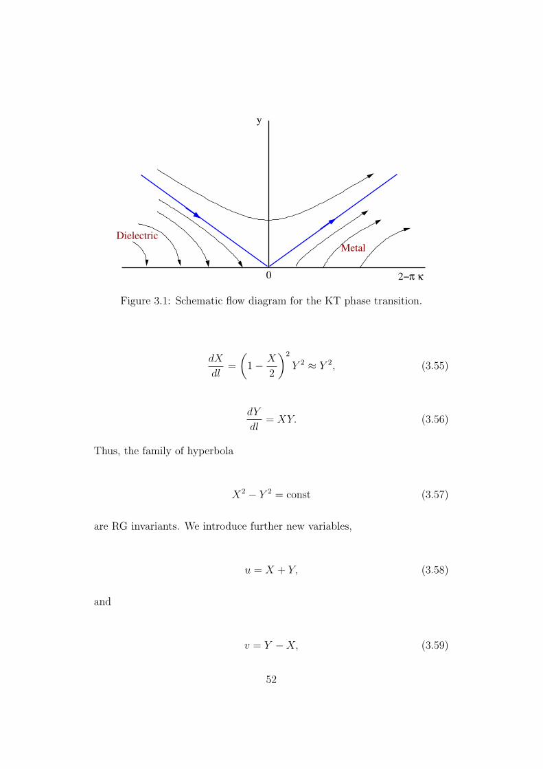
Eq. (3.53) has a fixed point at κc = 2/π, which corresponds precisely to

the critical temperature Tc = π/2 obtained before. However, Eqs. (3.52) and

(3.53) contain additional information. The flow diagram actually features a

line of fixed points for κ > κc at zero fugacity. Usually we say that the KT

flow diagram has a fixed line rather than a fixed point. The RG flow diagram

is shown in Fig. 3.1. Note that the we set 2−πκ as the horizontal axis, such

that the critical point occurs for a vanishing abscisse. The blue line shown

in the figure is a separatrix delimitating three different regimes. Below the

separatrix and for 2 − πκ < 0 we have a dielectric phase of vortices, which

corresponds to the low temperature regime where a vortex-antivortex pair is

tightly bound, forming in this way a dipole. The dielectric phase is gapless

because dipoles do not screen [31]. That is the reason why for 2 − πκ < 0

there is a fixed line. At a fixed point all modes are gapless, so if there is a line

of fixed points, like in the KT case, the excitation spectrum is completely

gapless along this line. For 2− πκ > 0, on the other hand, Debye screening

occurs and a gap arises. This is a (classical) metallic phase (or plasma phase)

of vortices.

Let us study in more detail the RG equations. To this end we introduce

the new variables,

X = 2− πκ, Y =2√πy. (3.54)

The RG equations become

51

2−π κ

y

Metal

Dielectric

0

Figure 3.1: Schematic flow diagram for the KT phase transition.

dX

dl=

(1− X

2

)2

Y 2 ≈ Y 2, (3.55)

dY

dl= XY. (3.56)

Thus, the family of hyperbola

X2 − Y 2 = const (3.57)

are RG invariants. We introduce further new variables,

u = X + Y, (3.58)

and

v = Y −X, (3.59)

52

such that the RG invariance equation becomes

u(l)v(l) = u0v0, (3.60)

where u0 = u(0) and v0 = v(0) are given initial conditions. Thus,

du

dl=

1

2(uv + u2)

=1

2(u0v0 + u2). (3.61)

It is straightforward to solve the above equation by direct integration. The

result is

arctan

(u

√u0v0

)− arctan

(u0√u0v0

)= 2√u0v0 ln

(ra

). (3.62)

Now we set r = ξ, i.e., we let the distance scale be equal to the correlation

length. In this case we have that the mass gap is approximately given by

ξ−1 ≈ exp

(− const√

T − Tc

), (3.63)

which is a result characteristic of the KT transition. Note that we do not

obtain in this case a power law for the mass gap.

For d > 2 the situation is completely different. First of all, the Coulomb

gas cannot be interpreted as vortices any longer, since in three dimensions

vortices are one-dimensional objects, lines or loops [2]. However, there are

53

physical systems in three dimensions with point-like topological defects where

an analysis similar to the one made here is applicable. For example, there

are systems where magnetic monopole-like defects occur in three spacetime

dimensions [28, 29, 32, 33, 34, 35, 36, 37, 38, 39, 40, 41]. Second, for d > 2

the RG equations (3.50) and (3.51) do not have nontrivial fixed points. Thus,

no phase transition occurs in this case. The excitation spectrum is always

gapped, so that the system remains permanently in the plasma phase.

54

Chapter 4

Bose-Einstein condensation and

superfluidity

4.1 Bose-Einstein condensation in an ideal gas

The Lagrangian for an ideal Bose gas is written in the imaginary time for-

malism as

L = b∗∂τb− µ|b|2 +1

2m∇b∗ · ∇b. (4.1)

All thermodynamic properties of the ideal Bose gas can be derived from the

partition function, which is given by the functional integral representation,

Z =

∫Db∗Db e−S, (4.2)

where

55

S =

∫ β

0

dτ

∫ddrL. (4.3)

The functional integral above is to be solved using periodic boundary condi-

tions b(0) = b(β) and b∗(0) = b∗(β).

We see from the action for the ideal Bose gas that the case µ = 0 is

special. Indeed, if µ = 0, the action is invariant by a transformation where

the Bose field is shifted by a constant, b → b + c. Note that the periodic

boundary conditions make the contribution c∗∂τb vanish. Thus, the special

role of the µ = 0 regime can be accounted for by shifting the Bose field by a

constant, i.e.,

b = b0 + b, (4.4)

and we require that b0 minimizes the action. This requirement implies that

no term linear in b or b∗ appears in the action. This is only true provided

µb0 = 0. (4.5)

This equation is fulfilled either for b0 = 0 and µ 6= 0, or b0 6= 0 and µ = 0.

The Lagrangian is rewritten as

L = −µ|b0|2 + b∗(∂τ − µ−

1

2m∇2

)b, (4.6)

where the Laplacian term is obtained through partial integration in the ac-

tion. By performing the Gaussian functional integral over b, we obtain, up

to a constant, the result,

56

Z ∼ exp(βV µ|b0|2)

det(∂τ − µ− 1

2m∇2) , (4.7)

where V is the (infinite) volume. Thus, the free energy density is given by,

f = − 1

βVlnZ

= −µ|b0|2 +1

βVln det

(∂τ − µ−

1

2m∇2

). (4.8)

Since the determinant of an operator is given by the product of the eigenval-

ues of the operator, we have to solve the differential equation,

(∂τ − µ−

1

2m∇2

)ψ = Eψ, (4.9)

where E is the eigenvalue. The equation above should be solved with periodic

boundary conditions ψ(0) = ψ(β). In order to solve the eigenvalue problem

we perform a Fourier transformation in the spatial variables,

ψ(τ, r) =

∫ddr

(2π)deip·rψ(τ,p). (4.10)

In this way the partial differential equation becomes an ordinary differential

equation of first order,

(∂τ − µ+

p2

2m

)ψ(τ,p) = Eψ(τ,p), (4.11)

which can be easily solved to obtain,

57

ψ(τ,p) = ψ(0,p) exp

[τ

(E + µ− p2

2m

)]. (4.12)

Due to the periodic boundary condition, the above equation for τ = β be-

comes

1 = exp

[β

(E + µ− p2

2m

)]. (4.13)

This implies,

En(p) = −iωn − µ+p2

2m, (4.14)

where ωn = 2πn/β with n ∈ Z is the so called Matsubara frequency. Inserting

these eigenvalues in Eq. (4.8) yields,

f = −µ|b0|2 +1

β

∞∑n=−∞

∫ddp

(2π)dln

(−iωn − µ+

p2

2m

). (4.15)

Our interest is to compute the particle density, n, which is the variable

conjugated to the chemical potential. We have,

n = −∂f∂µ, (4.16)

which yields,

n = |b0|2 −1

β

∞∑n=−∞

∫ddp

(2π)d1

iωn + µ− p2

2m

. (4.17)

In order to have b0 6= 0 we need µ = 0, so that the above equation becomes

for b0 6= 0,

58

n = |b0|2 −1

β

∞∑n=−∞

∫ddp

(2π)d1

iωn − p2

2m

. (4.18)

The Matsubara sum appearing above is performed in the Appendix D. Thus,

n = |b0|2 +

∫ddp

(2π)d1

eβp2

2m − 1.. (4.19)

The remaining integral is over a Bose distribution for free bosons in d di-

mensions. An integral involving a more general spectrum is evaluated in

Appendix C. Using Eq. (C.9) with z = 2 and c = 1/(2m) and making some

simplifications, we obtain,

|b0|2 = n

[1− ζ(d/2)

n

(mT

2π

)d/2]. (4.20)

Note that we have solved for |b0|2, which is the so called condensate density.

Its physical meaning is that for µ = 0 the particle density zero momentum

gets depleted due to temperature effects. The density at zero momentum

emerges because in momentum and frequency space,

b(ωn,p) = b0δd(p)δn,0 + b(ωn,p), (4.21)

such that b0 is associated to the zero momentum and zero Matsubara mode

contribution of the Bose field. The Bose-Einstein condensation is thus the

macroscopic occupation of the zero momentum state, in which case b repre-

sents the fluctuation around the condensate.

Eq. (4.20) can be rewritten as

59

|b0|2 = n

[1−

(T

Tc

)d/2], (4.22)

where

Tc =2π

m

[n

ζ(d/2)

]2/d

, (4.23)

is the critical temperature. For T = Tc the condensate vanishes. Note that

for T = 0 all the particles are condensed. This is a feature of the ideal Bose

gas. We will see that in the interacting case the condensate is also depleted

at T = 0 due to the interaction.

From the expression for the critical temperature we see that it vanishes

for d = 2, implying that no condensate exists in a two-dimensional ideal Bose

gas at finite temperature. This result is actually more general and holds even

in the interacting case. It is known as Hohenberg’s theorem [19].

4.2 The dilute Bose gas in the large N limit

In Chapter 2 we have studied the O(n) classical non-linear σ model in the

large n limit. We will now use this knowledge to perform a 1/N expansion

for an interacting Bose gas. Such an expansion actually corresponds to the so

called random phase approximation (RPA) for the dilute Bose gas introduced

long time ago [49, 50, 52, 53, 54]. That the 1/N expansion for the dilute Bose

gas corresponds to RPA was recognized by Kondor and Szepfalusy [53] long

time ago. Their analysis will be revisited here from a functional integral

point of view [43].

60

4.2.1 The saddle-point approximation

Let us consider the following action for a N -component interacting Bose gas:

S =

∫ β

0

dτ

∫ddr

N∑α=1

b∗α

(∂τ − µ−

∇2

2m

)bα +

g

2

(N∑α=1

|bα|2)2 , (4.24)

where bα and b∗α are complex commuting fields. The partition function is

then given by

Z =

∫ [∏α

Db∗αDbα

]e−S. (4.25)

In order to perform the 1/N -expansion we introduce an auxiliary field λ(τ, r)

via a Hubbard-Stratonovich transformation:

S ′ =

∫ β

0

dτ

∫ddr

[N∑α=1

b∗α

(∂τ − µ−

∇2

2m+ iλ

)bα +

1

2gλ2

]. (4.26)

Now we integrate out N − 1 Bose fields to obtain the effective action

Seff = (N − 1)Tr ln

(∂τ − µ−

∇2

2m+ iλ

)+

∫ β

0

dτ

∫ddr

[b∗(∂τ − µ−

∇2

2m+ iλ

)b+

1

2gλ2

], (4.27)

where we have called b the unintegrated Bose field.

Next we extremize the action according to the saddle-point approxima-

61

tion (SPA), a procedure that becomes exact for N → ∞. This part of the

calculation is practically identical with the one for the ideal Bose gas. This

is done by making the replacement iλ → λ0 and b → b0, with λ0 and b0 be-

ing constant fields, followed by extremization with respect to these constant

background fields. From this SPA we obtain the equations

(λ0 − µ)b0 = 0, (4.28)

λ0 = g|b0|2 −Ng

β

∞∑n=−∞

∫ddp

(2π)d1

iωn + µ− λ0 − p2

2m

. (4.29)

The large N limit is taken with Ng fixed. Below the critical temperature

Tc we have b0 6= 0, and thus from Eq. (4.28) λ0 = µ. Therefore, Eq. (4.29)

becomes

|b0|2 =µ

g−N

(m

2πβ

)d/2ζ(d/2), (4.30)

provided d > 2. The second term on the RHS of thee above equation is, up to

the prefactor N , the same as the one in Eq. (4.20) for the condensate density

of the ideal Bose gas. The particle density is obtained as usual n = −∂f/∂µ,

where f = − lnZ/(NV β) is the free energy density. This gives us

n =|b0|2

N+

∫ddp

(2π)d1

exp[β(

p2

2m+ λ0 − µ

)]− 1

. (4.31)

By setting λ0 = µ in Eq. (4.31) and using Eq. (4.30), we obtain

62

n =µ

Ng, (4.32)

and therefore the condensate density becomes,

n0 ≡|b0|2

N= n

[1−

(T

Tc

)d/2], (4.33)

where

Tc =2π

m

[n

ζ(d/2)

]2/d

. (4.34)

We see that the SPA does not change the value of Tc with respect to the

non-interacting Bose gas. Indeed, the SPA corresponds to the Hartree ap-

proximation and it is well known that it gives a zero Tc shift.

4.2.2 Gaussian fluctuations around the saddle-point ap-

proximation: Bogoliubov theory and beyond

In order to integrate out λ approximately, we consider the 1/N -corrections

to the SPA by computing the fluctuations around the constant background

fields b0 and λ0. By setting

b = b0 + b, iλ = λ0 + iλ, (4.35)

and expanding the effective action (4.27) up to quadratic order in the λ field,

we obtain

63

Seff = SSPAeff +

∫ β

0

dτ

∫ddr

[b∗(∂τ − µ+ λ0 −

∇2

2m

)b+ iλ(b∗0b+ b0b

∗ + |b|2) +1

2gλ2

]−N

2

∫ β

0

dτ

∫ β

0

dτ ′∫ddr

∫ddr′λ(τ, r)G0(τ − τ ′, r− r′)G0(τ ′ − τ, r′ − r)λ(τ ′, r′), (4.36)

where SSPAeff is the effective action (4.27) in the SPA and

G0(τ, r) =1

β

∞∑n=−∞

∫ddp

(2π)dei(p·r−ωnτ)G0(iωn,p), (4.37)

with

G0(iωn,p) =1

iωn + µ− λ0 − p2

2m

. (4.38)

After integrating out λ the effective action can be cast in the form

Seff = SSPAeff +

1

2Tr ln

[δ(τ − τ ′)δd(r− r′)−Ng G0(τ − τ ′, r− r′)G0(τ ′ − τ, r′ − r)

]+

1

2

∫ β

0

dτ

∫ddr

∫ β

0

dτ ′∫ddr′ Ψ†(τ, r)M(τ − τ ′, r− r′)Ψ(τ, r′)

+b∗02

∫ β

0

dτ

∫ddr

∫ β

0

dτ ′∫ddr′

[1 0

]Ψ(τ, r)Γ(τ − τ ′, r− r′)Ψ†(τ ′, r′)Ψ(τ ′, r′)

+b0

2

∫ β

0

dτ

∫ddr

∫ β

0

dτ ′∫ddr′ Ψ†(τ, r)

1

0

Γ(τ − τ ′, r− r′)Ψ†(τ ′, r′)Ψ(τ ′, r′)

+1

8

∫ β

0

dτ

∫ddr

∫ β

0

dτ ′∫ddr′Ψ†(τ, r)Ψ(τ, r)Γ(τ − τ ′, r− r′)Ψ†(τ ′, r′)Ψ(τ ′, r′),(4.39)

where we have introduced the two-component fields

64

Ψ†(τ, r) =

[b∗(τ, r) b(τ, r)

], Ψ(τ, r) =

b(τ, r)

b∗(τ, r)

, (4.40)

which satisfy Ψ†Ψ = 2|b|2. The matrix M(τ − τ ′, r − r′) has a Fourier

transform given by

M(iωn,p) =

−iωn + E(ωn,p) b20 Γ(iωn,p)

(b∗0)2Γ(iωn,p) iωn + E(ωn,p)

, (4.41)

where

E(ωn,p) = −µ+ λ0 +p2

2m+ |b0|2Γ(iωn,p), (4.42)

with

Γ(iωn,p) =g

1−NgΠ(iωn,p), (4.43)

which is the Fourier transform of the effective interaction Γ(τ − τ ′, r − r′),

and

Π(iωn,p) =1

β

∞∑m=−∞

∫ddq

(2π)dG0(iωn + iωm,p + q)G0(iωm,q), (4.44)

is the polarization bubble. The effective interaction can be represented in

terms of Feynman diagrams as in Fig. 4.1. Physically λ corresponds to the

65

= +

+ + ...

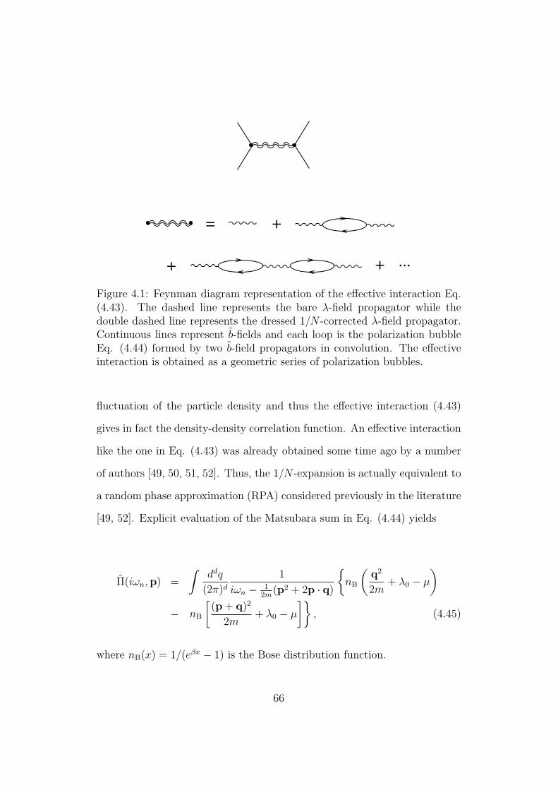
Figure 4.1: Feynman diagram representation of the effective interaction Eq.(4.43). The dashed line represents the bare λ-field propagator while thedouble dashed line represents the dressed 1/N -corrected λ-field propagator.Continuous lines represent b-fields and each loop is the polarization bubbleEq. (4.44) formed by two b-field propagators in convolution. The effectiveinteraction is obtained as a geometric series of polarization bubbles.

fluctuation of the particle density and thus the effective interaction (4.43)

gives in fact the density-density correlation function. An effective interaction

like the one in Eq. (4.43) was already obtained some time ago by a number

of authors [49, 50, 51, 52]. Thus, the 1/N -expansion is actually equivalent to

a random phase approximation (RPA) considered previously in the literature

[49, 52]. Explicit evaluation of the Matsubara sum in Eq. (4.44) yields

Π(iωn,p) =

∫ddq

(2π)d1

iωn − 12m

(p2 + 2p · q)

{nB

(q2

2m+ λ0 − µ

)− nB

[(p + q)2

2m+ λ0 − µ

]}, (4.45)

where nB(x) = 1/(eβx − 1) is the Bose distribution function.

66

By inverting the matrix (5.31) we obtain the propagator

G(iωn,p) =

Gb∗b(iωn,p) Fb∗b∗(iωn,p)

Fbb(iωn,p) Gb∗b(−iωn,p)

, (4.46)

where

Gb∗b(iωn,p) =iωn + λ0 − µ+ p2

2m+ |b0|2Γ(iωn,p)

ω2n +

[p2

2m+ λ0 − µ+ |b0|2Γ(iωn,p)

]2

− |b0|4Γ2(iωn,p),

(4.47)

and

Fb∗b∗(iωn,p) = − (b∗0)2Γ(iωn,p)

ω2n +

[p2

2m+ λ0 − µ+ |b0|2Γ(iωn,p)

]2

− |b0|4Γ2(iωn,p),

(4.48)

is the anomalous propagator.

For T > Tc we have that b0 = 0 and the matrix propagator becomes diag-

onal. In this case if we neglect the interaction terms from the effective action

(4.39), the b propagator corresponds to the Hartree approximation. Thus,

above Tc we have to consider the effective interaction between the bosons in

Eq. (4.39) in order to obtain a nontrivial result for the excitation spectrum.

This is achieved by computing the 1/N -correction to the propagator. Below

Tc, however, a nontrivial result for the excitation spectrum is obtained from

the pole of the propagator even without considering the 1/N correction to

it. This is easily seen from the structure of the propagators (4.47) and (4.48)

67

where the effective interaction Γ(iωn,p) appears explicitly. Above Tc the ef-

fective interaction appears in the propagator only in the next to the leading

order in 1/N .

4.2.3 The excitation spectrum below Tc

As we have discussed in the previous Subsection, below Tc a nontrivial re-

sult for the excitation spectrum is obtained in an approximation where the

interaction term of the effective action is neglected. Thus, we now undertake

a study of the spectrum of the system in such a Gaussian approximation.

Later we shall see that the effective action in the Gaussian approximation

gives the free energy density up to the order 1/N .

From the pole of the matrix propagator (4.46) we obtain that the energy

spectrum E(p) satisfy the equation

E2(p) = Re

{p2

2m+ λ0 − µ+ |b0|2Γ[E(p) + iδ,p]

}2

− |b0|4Re Γ2[E(p) + iδ,p]

=

(p2

2m+ λ0 − µ

)2

+ 2

(p2

2m+ λ0 − µ

)|b0|2Re Γ[E(p) + iδ,p], (4.49)

where δ → 0+. Note that Eq. (4.49) can be written as the product of two

elementary excitations, E2(p) = El(p)Et(p), where

El(p) =p2

2m+ λ0 − µ+ 2|b0|2Re Γ[E(p) + iδ,p], (4.50)

Et(p) =p2

2m+ λ0 − µ, (4.51)

68

are the spectrum of the longitudinal and transverse modes, respectively.

When λ0 = µ we obtain that the transverse mode is gapless, consistent

with Goldstone theorem.

By inserting the saddle-point value λ0 = µ, we obtain the following self-

consistent equation for the excitation spectrum

E(p) =

√p4

4m2+|b0|2m

p2 ReΓ[E(p) + iδ,p], (4.52)

where the notation E(p) ≡ E(p)|λ0=µ is used. Note that the above spectrum

corresponds to a generalization of the well known Bogoliubov spectrum [48].

The difference lies in the fact that in the 1/N -expansion the coupling con-

stant g is replaced by the effective interaction Γ[E(p) + iδ,p] [49, 50]. At

zero temperature Π(iω,p) vanishes and the excitation spectrum corresponds

to the usual Bogoliubov spectrum. As we shall see, the modification of the

spectrum by the effective interaction accounts for thermal fluctuation effects

in higher temperatures and allows us a consistent treatment of critical fluc-

tuations near Tc.

In Eq. (4.52) we can legitimately replace |b0|2 by Nn, since the error

committed in such a replacement is of higher order in 1/N . Thus, Eq. (4.52)

becomes

E(p) =

√p4

4m2+nN

mp2 ReΓ[E(p) + iδ,p]. (4.53)

Note that since Γ[E(p) + iδ,p] ∼ O(1/N), Eq. (4.53) is independent of N

for N →∞.

In order to obtain the spectrum of elementary excitations we need to

69

evaluate the polarization bubble (4.45). Unfortunately, it cannot be evalu-

ated exactly, although many of its properties and asymptotic limits can be

worked out exactly [52, 55]. For instance, for distances much larger than the

thermal wavelength the polarization bubble can be evaluated exactly [52, 55].

This is called the classical limit in the early literature of the field. In the

classical limit we can approximate the Bose distribution in Eq. (4.45) by

nB(x) ≈ 1/βx. In such a limit we can write

Π(iωn,p) = Π0(p) + Π1(iωn,p), (4.54)

where

Π0(p) = −4m2T

∫ddq

(2π)d1

[(p + q)2 + 2m(λ0 − µ)][q2 + 2m(λ0 − µ)],

(4.55)

Π1(iωn,p) = 8m3Tiωn

∫ddq

(2π)d1

2miωn − p2 − 2p · q

× 1

[(p + q)2 + 2m(λ0 − µ)][q2 + 2m(λ0 − µ)]. (4.56)

Setting λ0 = µ, we obtain the following result for the effective interaction:

Γ0(p) =g

1 + αdTm2Ngpd−4, (4.57)

where p ≡ |p| and

70

αd =Γ(2− d/2)Γ2(d/2− 1)

2d−2πd/2Γ(d− 2). (4.58)

When 2 < d < 4 we obtain for small p that Γ0(p) ≈ p4−d/(αdTm2N), such

that the excitation spectrum is given approximately by

E(p) ≈√

n

αdm3Tp(6−d)/2. (4.59)

The above equation reflects the dynamic scaling behavior, E(p) ∼ pz of the

excitation spectrum, where z is the dynamic critical exponent. Thus, from

Eq. (4.59) we see that it implies a dynamic exponent

z =6− d

2. (4.60)

At d = 3 we obtain z = 3/2, which is the expected result for 4He. This

result was obtained first by Patashinskii and Pokrovskii [56]. Note that

the same order in 1/N when Tc is approached from above fails to give a

non-trivial dynamic scaling behavior. Only after taking into account non-

Gaussian Gaussian fluctuations, corresponding to the next-to-leading order in

1/N , is possible to obtain a non-trivial dynamic exponent. The origin of this

non-symmetric critical behavior comes from the intrinsic existing asymmetry

in the dilute Bose gas with respect to the ordered and disordered phases.

Indeed, in the ordered phase the spectrum has a relativistic-like form, while

in the disordered phase the non-relativistic behavior dominates the physics.

The static critical exponents are not affected by this asymmetric behavior

of the theory, but the critical dynamics properties are. Note that our value

71

of the dynamic exponent is independent of N , i.e., z = (6 − d)/2. This

exponent agrees with model F critical dynamics only at d = 3. There the

dynamic exponent is given exactly by z = d/2 [70]. At d = 3 the value of z is

indeed expected to be z = 3/2 [57]. However, a word of caution is necessary

here. Our calculation of the dynamic exponent was made assuming that finite

temperature dynamics can be derived out of a quantum Hamiltonian using

equilibrium statistical mechanics. This is not quite right. Critical dynamics

cannot be derived from a Hamiltonian and equilibrium statistical mechanics

analysis [70].

The full classical theory, including dynamical effects, should account for

the frequency dependence of Π(iωn,p). The full expression for Π(iωn,p) in

the classical approximation and 2 < d < 4 is [53]

Π(iωn,p) = −Adm2Tpd−4

[(1− 2miωn

p2

)d−3

+ e−iπ(d−2)

(1 +

2miωnp2

)d−3],

(4.61)

where

Ad = 22−dπ−d/2eiπ(d−2)/2Γ(d/2− 1)Γ(3− d). (4.62)

The derivation of Eq. (4.61) is made in Appendix E. As ωn → 0 Eq. (4.61)

reduces correctly to Π(0,p) = Π0(p) = −αdTm2pd−4 and we recover Eq.

(4.57) for the effective interaction.

For d = 3 Eq. (4.61) becomes

72

Π(iωn,p) = −iTm2

2πpln

(2miωn + p2

2miωn − p2

). (4.63)

By making the replacement iωn → E(p) + iδ and substituting in Eq. (4.53),

we obtain after taking the real part of the effective interaction the following

expression for the excitation spectrum

E(p) =p2

2m

1 +4mnNg

p2 +(Tm2Ng

2πln∣∣∣2m eE(p)+p2

2m eE(p)−p2

∣∣∣)2

1/2

. (4.64)

4.2.4 Depletion of the condensate

At T = 0 the depletion of the condensate is more easily obtained from the

formula

n =1

N(|b0|2 + 〈|b|2〉) = n0 +

1

N〈|b|2〉, (4.65)

where

〈|b|2〉 = limε→0+

∫ ∞−∞

dω

2π

∫ddp

(2π)dGb∗b(iω,p)eiωε. (4.66)

Note that for T = 0 the polarization bubble vanishes and we can set Γ(iω, p) =

g. Explicit evaluation of the ω-integral in Eq. (4.66) yields

〈|b|2〉 =

∫ddp

(2π)d

[p2

2m+ nNg

2E(p)− 1

2

], (4.67)

where E(p) =√

p4/4m2 + nNgp2/m. The integral in Eq. (4.67) can be

easily evaluated using dimensional regularization [44], so that the factor 1/2

73

between brackets does not contribute. Thus, we can rewrite Eq. (4.67) as

〈|b|2〉 =1

2

(A+

M2

2B

), (4.68)

where M2 = 4mnNg and

A =

∫ddp

(2π)dp√

p2 +M2, (4.69)

and

B =

∫ddp

(2π)d1

p√p2 +M2

. (4.70)

The integrals A and B are related to the integral

Iα(d) =

∫ddp

(2π)d1

(p2 +M2)α, (4.71)

by

A =2√πΓ(d+1

2

)Γ(d/2)

I1/2(d+ 1), (4.72)

and

B =Γ(d−1

2

)2√πΓ(d/2)

I1/2(d− 1). (4.73)

The integral Iα can be evaluated with the usually tricks already employed in

Chapter 2. We have evaluated it in Appendix B. The result is given in Eq.

(B.13). Thus, ,

74

〈|b|2〉 =(mnNg/π)d/2

2√πΓ(d/2)

[Γ

(−d

2

)Γ

(d+ 1

2

)+

1

2Γ

(1− d

2

)Γ

(d− 1

2

)].

(4.74)

From the relation Γ(z + 1) = zΓ(z), we have

Γ

(1− d

2

)= −d

2Γ

(−d

2

), (4.75)

Γ

(d+ 1

2

)= Γ

(d− 1

2+ 1

)=d− 1

2Γ

(d− 1

2

), (4.76)

such that

〈|b|2〉 =(mnNg/π)d/2(d− 2)

8√πΓ(d/2)

Γ

(−d

2

)Γ

(d− 1

2

). (4.77)

It can be shown that for 2 < d < 4 the coupling g is given in terms of the

s-wave scattering length by [46]

g =4πd/2ad−2

Γ(d/2− 1)m. (4.78)

For d = 3 this yields the well-known formula g = 4πa/m. Setting d = 3

finally yields

n0 = n

(1− 8

3

√Nna3

π

), (4.79)

which for N = 1 is the usual Bogoliubiv’s formula for the depletion of the

condensate [48].

75

4.2.5 The superfluid density

In order to calculate the superfluid density, we have to perform a Galilei

boost in the system [58]. A normal fluid is insensitive to a Galilei boost

but a superfluid is not. This fact imposes strong constraints on the form

of the excitation spectrum of a superfluid [47]. For instance, it implies that

an ideal Bose gas in its condensed phase is not a superfluid, although we

sometimes speak in this case of “ideal superfluidity”, since the calculation of

the superfluid density using the standard definition implies in this case that

it is identical to the condensate density. This is absolutely not the case in

general. Indeed, superfluidity may occur even when no Bose condensation

is possible, as for example in the case of two-dimensional interacting Bose

systems at finite temperature, where the Hohenberg-Mermin-Wagner [19, 20]

theorem forbids the appearance of a Bose condensate. In this situation there

is a phase transition to a superfluid state without spontaneous symmetry

breaking, which is the Kosterlitz-Thouless phase transition [21] discussed in

Chap. 3. Another example comes from three-dimensional superfluids. It

is easy to show that for a homogeneous superfluid at zero temperature the

superfluid density corresponds to the whole density [69], while the condensate

is depleted due to interaction effects [47, 48]. Experimentally it is estimated

that for 4He in three dimensions and at zero temperature the condensate

fraction is about 13% [59], although the whole system is superfluid.

A Galilei boost of momentum k0 changes the Lagrangian to

Lk0 = L+k2

0

2m|b|2 + k0 · j, (4.80)

76

where

j = − i

2m(b∗∇b− b∇b∗) (4.81)

is the current density.

The free-energy density in the presence of the Galilei boost is given by

the functional integral

Fk0 = −TV

[ln

∫Db∗Dbe−

R β0 dτ

RddrLk0

]. (4.82)

The superfluid density is defined by [58]

ρs = m2 limk0→0

∂2Fk0

∂k20

. (4.83)

It is now easy to show that

ρs = m〈|b|2〉 − m2

d

∫ β

0

dτ

∫ddrC(τ, r), (4.84)

where

C(τ, r) = 〈j(τ, r) · j(0, 0)〉 − 〈j(τ, r)〉 · 〈j(0, 0)〉 (4.85)

is the connected current correlation function and the factor 1/d in Eq. (4.84)

emerges due to rotational invariance. Note that 〈|b|2〉 is the total density of

the fluid and sometimes we define ρ = m〈|b|2〉 as the total fluid density.

As an example, let us calculate the superfluid density for the Lagrangian

(4.80) in a regime where the non-Gaussian fluctuations are small using a

77

Bogoliubov transformation [48] for the Lagrangian (4.80). We will not con-

sider the effects of vortices, which is certainly important when perfoming

calculations using directly the phase of the order parameter [2, 21].

In the Bogoliubov approximation the superfluid density is given by

ρs = ρ− T

4d

∞∑n=−∞

∫ddk

(2π)dk2[G2(ωn,k)− |F (ωn,k)|2

], (4.86)

where we the Green functions are given by the zero temperature counterpart

of the Green functions (4.47) and (4.48), which we write as

G(ωn,k) =iωn + k2

2m+ gρ

m

ω2n +

(k2

2m

)2+ gρ

m2 k2, (4.87)

and

F (ωn,k) =gb2

0

ω2n +

(k2

2m

)2+ gρ

m2 k2. (4.88)

In the above equation b0 = 〈b〉 and we are approximately setting 〈|b|2〉 ≈ |b0|2,

which is true up to higher order effects.

The above integral and Matsubara sum can be calculated exactly if we

assume a low-energy approximation to the Bogoliubov spectrum, i.e.,

E(k) ≈ c|k|, (4.89)

where c2 = gρ/m2. Thus, by rescaling the momenta to remove the c factor,

the expression for the normal fluid density (note that ρs = ρ− ρn) becomes

78

ρn =T

cd+2d

∞∑n=−∞

∫ddk

(2π)dk2

ω2n + k2

− 2T

cd+2d

∞∑n=−∞

∫ddk

(2π)dk2ω2

n

(ω2n + k2)2

, (4.90)

which can be rewritten as

ρn =T

cd+2d

∫0<|k|<Λ

ddk

(2π)d+

T

cd+2d

∞∑n6=0

∫ddk

(2π)dk2

ω2n + k2

− 2T

cd+2d

∞∑n=−∞

∫ddk

(2π)dk2ω2

n

(ω2n + k2)2

. (4.91)

It is convenient in this case to perform the integrations first, and only

afterwards evaluate the Matsubara sums. The first and second integrals in

ρn can be related to the integrals I1 and I2 evaluated in the Appendix B,

where ω2n plays the role of M2. We only need to notice that

∫ddk

(2π)dk2

(k2 +M2)α= 2πd Iα(d+ 2), (4.92)

where α = 1, 2. Note that we have to replace d → d + 2 in the integrals I1

and I2 of Appendix B. Thus,

∫ddk

(2π)dk2

ω2n + k2

= −πd/2T d

dΓ

(1− d

2

)|n|d. (4.93)

Now the sum can be easily performed by using the definition of the zeta

function (see Appendix C), so that we obtain,

79

T∞∑n6=0

∫ddk

(2π)dk2

ω2n + k2

= −2πd/2T d+1

dΓ

(1− d

2

)ζ(−d). (4.94)

The remaining integral along with the Matsubara sum in ρn is easily eval-

uated using a similar procedure. Therefore, after some simplifications, the

final result for the superfluid density is

ρs = ρ− 2md+2

(gρ)1+d/2d

[ΛdT

(4π)d/2dΓ(d/2)

− (d+ 1)πd/2Γ

(1− d

2

)ζ(−d)T d+1

], (4.95)

where Λ is an ultraviolet cutoff which is of the order of the inverse scattering

length, Λ ∼ a−1. The term linear in the temperature arises also in a mean-

field calculation of the stiffness in the classical XY model [60]. The term

proportional to T d+1 is a quantum correction due to phonon excitations of

the Bose liquid [47]. The Landau formula usually only gives the contribution

proportional to T d+1.

For d = 2 we have

ρs = ρ− m4

2π(gρ)2

[Λ2T

4+ 3ζ(3)T 3

], (4.96)

while for d = 3 we obtain

ρs = ρ− 2m5

9(gρ)5/2

(Λ3T

4π2+π2

5T 4

). (4.97)

80

It should be noted that for d = 2 the coupling g itself is density dependent,

being given by [61]

g = − 4π

m ln(e2γρa2

4m

) , (4.98)

where γ is the Euler constant and the naive diluteness condition ρad/m� 1

has to be modified for d = 2 to ln ln[m/(ρa2)] � 1 [62]. This is in contrast

with the d = 3 case where g = 4πa/m, with no dependence on the the total

density.

81

Chapter 5

Mott insulators

5.1 The Hubbard model

The simplest electronic model of a Mott insulator is provided by the so called

Hubbard model:

H = −t∑〈i,j〉

∑σ

f †iσfjσ − µ∑i,σ

niσ + U∑i

ni↑ni↓, (5.1)

where fiσ is a fermion in the lattice, niσ ≡ f †iσfiσ, and σ =↑, ↓. In the above

Hamiltonian t, U > 0, and µ is the chemical potential. In the kinetic term

the lattice sum runs only nearest neighbors only. The Hubbard Hamiltonian

is exactly solvable in the limits U = 0 and t = 0. The non-interacting limit

corresponds to band theory in the tight-binding approximation, while the

t = 0 limit corresponds to the atomic limit. Although in the atomic limit

the theory is interacting, it is easily diagonalizable, since

82

Ht=0 =∑i

hi, (5.2)

where

hi = −µ∑σ

niσ + U∑i

ni↑ni↓. (5.3)

Thus,

[hi, niα] = 0, (5.4)

and therefore the eigenstates of niα are also eigenstates of hi. In this case

we can simply omit the lattice sites of any calculation, since the sites are

decoupled. The eigenstates of the h are |0〉, | ↑〉, | ↓〉, and | ↑↓〉, correspond-

ing to empty, singly occupied (with either up or down spins), and doubly

occupied sites, respectively. The corresponding eigenenergies are ε0 = 0,

ε↑ = ε↓ = −µ, and ε2 = U − 2µ.

Let us consider the example of a half-filled band, i.e., the total number

of fermions in the system equals the number of lattice sites L. In this case

it can be shown that for a bipartite lattice1 µ = U/2 exactly. This result

is straightforwardly checked in the atomic limit. To see that this result is

also valid when t 6= 0, we just perform a particle-hole (ph) transformation

fiσ → eiQ·Rif †iσ, f †iσ → eiQ·Rifiσ, where Q = (π, ..., π). When µ = U/2 the

Hamiltonian is invariant under this particle-hole transformation. Note that

the factor eiQ·Ri is necessary in order to maintain the sign of the hopping

1This means that the lattice can be viewed as being made of two interpenetratingsublattices. One simple example is the cubic lattice

83

term, because fermions anticommute. Indeed, we have that eiQ·(Ri−Rj) = −1,

since Ri and Rj are nearest neighbor sites. Thus, the ph-transformation

yields in general the Hamiltonian

H ′ = U − 2µ− t∑〈i,j〉

∑σ

f †iσfjσ + (µ− U)∑σ

niσ + U∑i

ni↑ni↓ (5.5)

Note that the Hamiltonians H from Eq. (5.1) and the one given above

coincide for µ = U/2. Now let f and f ′ be the free energy densities of the

Hamiltonians H and H ′ given in Eqs. (5.1) and (5.5), respectively. We have

the particle density is given as usual by the thermodynamical relation

n = −∂f∂µ, (5.6)

while from f ′ we obtain,

2− n = −∂f′

∂µ. (5.7)

Since µ = U/2 implies H = H ′, we also have that f = f ′ for this value of

the chemical potential. Therefore, for µ = U/2 the RHS of both Eqs. (5.6)

and (5.7) are the same, so that we obtain n = 2− n, which yields n = 1.

At half-filling the Hubbard Hamiltonian can be rewritten as

H = −t∑〈i,j〉

∑σ

f †iσfjσ −2U

3

∑i

S2i , (5.8)

where

84

Si =1

2

∑α,β

f †iασαβfiβ, (5.9)

with σ ≡ (σ1, σ2, σ3), σi being the Pauli matrices. For U � t doubly occupied

sites are strongly suppressed and second-order perturbation theory yields the

effective Hamiltonian [3]

H =4t2

USi · Sj, (5.10)

subjected to the local constraint

∑σ

niσ = 1. (5.11)

Note the subtlety here. The half-filling condition demands that the particle

density

n =1

L

∑i,σ

〈niσ〉 = 1, (5.12)

which is easily enforced when µ = U/2. This is a global constraint, that

simply demands the average site occupation be the unity. However, when

U � t the average constraint becomes a local one given by the operator

equation (5.11), i.e., double occupation is strictly forbidden.

The effective Hamiltonian (5.10) is the one of a Heisenberg antiferromag-

net. It is rotational invariant in spin space, i.e., it has an SU(2) symmetry.

This means that the total spin operator

85

S =∑i

Si, (5.13)

commutes with the Hamiltonian. However, the ground state of the Heisen-

berg Hamiltonian breaks this symmetry. The most favorable state at zero

temperature corresponds to alternating spins in the lattice. This state is pic-

torially shown for a square lattice in Fig. 2.1. The antiferromagnetic state

shown in the figure is actually a mean-field state for the Heisenberg model,

the so called Neel state. This state is also a mean-field state of the Hubbard

model at half-filling. Incidentally, the total spin operator (5.13) obviously

commutes with the Hubbard Hamiltonian, showing that the Hubbard model

is SU(2) symmetric, as expected physically.

Let us perform the mean-field theory for the Hubbard model in a d-

dimensional cubic lattice explicitly. In order to do this, we introduce an

auxiliary field via a Hubbard-Stratonovich transformation:

H = −t∑〈i,j〉

∑σ

f †iσfjσ − U∑i

mi · Si +3U

8

∑i

m2i . (5.14)

We are looking for a mean-field state with a staggered magnetic moment

mi = eiQ·Rim, (5.15)

where the vector m is uniform. Rotational invariance allows us to fix a

direction for m. We will choose the quantization axis to be along the z-

direction. Thus, m = mez. Let us define

86

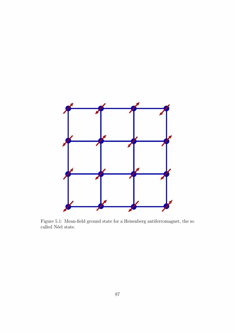
Figure 5.1: Mean-field ground state for a Heisenberg antiferromagnet, the socalled Neel state.

87

fiσ =

ciσ, i ∈ A

ciσ, i ∈ B(5.16)

The mean-field Hamiltonian can be written as

HMF =∑k,σ

ψ†kσMkσψkσ +3UL

8m2, (5.17)

where

ψkσ =

ckσ

ckσ

, ψ†kσ =

[c†kσ c†kσ

], (5.18)

and

Mkσ =

−σUm2

εk

εkσUm

2

, (5.19)

with the tight-binding dispersion

εk = −2td∑a=1

cos ka. (5.20)

The mean-field Hamiltonian is easily diagonalized and leads to the energy

spectrum

E±k = ±√ε2k +

U2m2

4, (5.21)

and we see that the electronic spectrum is gapped. Thus, the mean-field

ground state energy per site is

88

E0 = − 2

L

′∑k

E+k +

3U

8m2, (5.22)

where the prime on the sum over k is to denote that we are summing over

the upper half of the Brillouin zone. Let us specialize to two dimensions.

By minimizing the above equation with respect to m, we obtain the gap

equation,

3

2U=

∫ π

0

dkx2π

∫ π

0

dky2π

1

E+k

. (5.23)

In two dimensions it is not a too bad approximation, at least for more qual-

itative purposes, to use a square density of states to evaluate the above

momentum integral,

ρ(ε) =1

Wθ

(W

2− |ε|

), (5.24)

where W = 4t is the bandwidth and θ(x) is the Heaviside function. This

yields the magnetization,

m =2W

U

e−3W2U

1− e− 3WU

. (5.25)

Thus, mean-field theory predicts that at half-filling the Hubbard model is

an antiferromagnetic insulator for all U > 0. This is not quite accurate, of

course. For a small enough U the system should be a metal. Indeed, the

Hubbard model undergoes a metal insulator transition for a critical value of

the interaction typically of the order of the bandwidth W [64]. The metal-

insulator transition in the Hubbard model started to be better understood

89

with the use of the so called dynamical mean-field [65], which is based on the

large dimension limit of the Hubbard model [66]. For a thorough review on

the subject, see Ref. [65].

5.2 The Bose-Hubbard model

The Hamiltonian of the so called Bose-Hubbard model [67] is given by

H = −J∑〈i,j〉

b†i bj − µ∑i

ni +U

2

∑i

ni(ni − 1), (5.26)

where U, J > 0, ni ≡ b†i bi and µ is the chemical potential. The summations

are over the sites of a cubic lattice and the symbol 〈i, j〉 means a sum over

nearest neighbors. The operators bi obey the usual bosonic commutation

relations, i.e., [bi, b†j] = δij und [bi, bj] = [b†i , b

†j] = 0.

The aim of this tutorial is to provide an introduction to the theory of the

Bose-Hubbard model, which in the last years gained considerable experimen-

tal relevance in the context of Bose-Einstein condensation (BEC) [68].

What kind of phases we expect for the above model? Firstly, let us note

that the Hamiltonian (5.26) is simply a lattice version of the interacting Bose

gas Hamiltonian. Indeed, the hopping term is just a lattice derivative. Thus,

for small enough U we expect to obtain a superfluid featuring the well known

Bogoliubov spectrum. To see this, just write

bi = b0 + δbi, b†i = b∗0 + δb†i , (5.27)

90

where b0 represents the condensate and minimize the Hamiltonian, and δbi

are small fluctuations around the condensate. By keeping just the quadratic

fluctuations, it is easy to see that the Hamiltonian can be approximately

written as H = LE0 + δH (L is the number of lattice sites), with

E0 = −(

2dJ + µ+U

2

)n0 +

U

2n2

0, (5.28)

δH =1

2

∑k 6=0

Ψ†kMkΨk, (5.29)

where we have performed a Fourier transformation in the lattice and

Ψ†k =

[δb†k δb−k

], Ψk =

δbk

δb†−k

, (5.30)

Mk =

εk − µ− U/2 + 2Un0 Ub20

U(b∗0)2 εk − µ− U/2 + 2Un0

, (5.31)

with εk = −2J∑d

a=1 cos ka and n0 ≡ |b0|2. Due to the minimization condi-

tion we have

µ = −2dJ − U

2+ Un0. (5.32)

The above result follows easily by demanding that the linear terms in both

δbi and δb†i vanish. Alternatively it may be derived by simply minimizing E0

with respect to n0. The energy spectrum can be obtained by simply solving

the Heisenberg equations of motion. To this end we need the equations

i∂tδbk = [δbk, δH], i∂tδb†−k = [δb†−k, δH]. (5.33)

91

After straightforward evaluation of the commutators, we can rewrite the two

equations above as a single matrix equation:

iσ3∂tΨk = MkΨk, (5.34)

where σ3 is the third Pauli matrix. The Ansatz

Ψk(t) = e−iEktΨk(0) (5.35)

solves Eq. (5.34) provided det(Ekσ3 − Mk) = 0, or

Ek = ±√

(εk − µ− U/2 + 2Un0)2 − U2n20. (5.36)

Note that due to the form of the chemical potential (5.32), the above spec-

trum is gapless, i.e., Ek=0 = 0, as required by superfluidity.

The above results are valid for U small, i.e., U � J . So, what happens

now in the opposite limit, when U � J? This is a subtle question. In the

continuum limit exact arguments [69, 70] involving the Ward identities show

that at zero temperature the superfluid density is identical to the particle

density, and this for for all values of U . This means that at zero temperature

the whole system is in a superfluid state, although not every particle is con-

densed, since the condensate is depleted due to interaction effects. Does this

exact result also holds in the lattice? The answer is: it depends on whether

the particle density 〈n〉 is integer or not! For noninteger particle density, ap-

proaching the strong coupling limit from the weak coupling one by varying

J/U essentially does not change the superfluid characteristics of the system.

92

Thus, in this situation the system is still a superfluid for U � J . However,

for 〈n〉 = n ∈ N the situation is different. In this case the bosons will localize

for large enough U and the system will become an insulator, whose ground

state has n particles per site. In order to better understand how it actually

works, let us consider the eigenstates of the number operator (we omit the

site index for simplicity)

|n〉 =1√n!

(b†)n|0〉, (5.37)

and the coherent state

|z〉 = e−|z|2/2 exp(zb†)|0〉

= e−|z|2/2

∞∑n=0

zn√n!|n〉. (5.38)

Recall that for a coherent state b|z〉 = z|z〉. Let us consider for simplicity

a two-site problem. For this case let us assume that the system is in the

coherent state

|Φ〉 = |z1, z2〉. (5.39)

The expectation value of the Hamiltonian in this state is the energy

E(z1, z2) ≡ 〈Φ|H|Φ〉 = −J(z∗1z2 + z∗2z1) +∑i=1,2

[−µ|zi|2 +

U

2|zi|2(|zi|2 − 1)

].

(5.40)

In terms of zi =√nie

iϕi , where ni is the mean particle number at the site i,

93

Eq. (5.40) becomes

En1,n2(ϕ1, ϕ2) = −2J√n1n2 cos(ϕ1 − ϕ2) +

∑i=1,2

[−µni +

U

2ni(ni − 1)

].

(5.41)

The above energy is similar to the classical Hamiltonian of a Josephson junc-

tion [72]. In order to explore this similarity further, we rewrite Eq. (5.41)

as

E(∆n,∆ϕ) = −J√N2 − (∆n)2 cos ∆ϕ+

U

4(∆n)2 + EN , (5.42)

where N = n1 + n2 is the total number of particles of the system, ∆n ≡

n1 − n2, ∆ϕ ≡ ϕ1 − ϕ2, and

EN = −(µ+

U

2

)N +

U

4N2. (5.43)

The energy (5.42) corresponds precisely to the Hamiltonian describing a

two-level Bose-Einstein condensate via a Josephson junction as discussed

by Leggett [73]. In this case the variable ∆n plays the role of the momentum

conjugated to ∆ϕ. Therefore, the Josephson current is given by

∂t∆n = −J√N2 − (∆n)2 sin ∆ϕ. (5.44)

The Josephson effect implies superfluidity. Semiclassically, since ∆n and ∆ϕ

are canonically conjugated, we have the uncertainty relation [72]

∆n∆ϕ ∼ 1. (5.45)

94

The so called Josephson “phase-voltage” relation is here generalized to

∂t∆ϕ =U

2∆n+

J∆n√N2 − (∆n)2

cos ∆ϕ. (5.46)

Recall that in the case of superconductors we have ∂t∆ϕ = 2eV/~, where

the voltage V the same as the difference of chemical potential across the

junction. In the above equation the role of 2eV/~ is played by U∆n/2. The

second term is absent in the Josephson relation. This term appears in the

context of Josephson junctions in Bose-Einstein condensates [71].

If U � J , the second term in Eq. (5.42) will constraint n1 ≈ n2 and a

commensurate situation n1 = n2 = n = 1, 2, 3, . . . will be favored. It is then

clear that the current will be zero and we have an insulator.

Now we will solve the full model approximately using a Green function

method. The aim is to compute the Green function

Gij(t) = −i〈T [bi(t)b†j(0)]〉, (5.47)

where T [bi(t1)b†j(t2)] = θ(t1− t2)bi(t1)b†j(t2) + θ(t2− t1)b†j(t2)bi(t1) and θ(t) is

the Heaviside function. The Green function can be calculated exactly in both

limit cases J = 0 and U = 0. We will consider a solution that corresponds to

a perturbation expansion in J/U , i.e., around the limit case J = 0. Thus, we

have to compute the exact Green function in this limit in order to proceed.

The J = 0 limit is actually a single-site system, since the Hamiltonian

95

can be written as a sum of single-site Hamiltonians:

HJ=0 =∑i

hi, (5.48)

where

hi = −µni +U

2ni(ni − 1). (5.49)

In this case it is enough to compute the Green function for the single-site

Hamiltonian hi and the site index can even be omitted. Since [h, n] = 0, the

eigenstates |n〉 of n are the exact eigenstates of h with eigenvalues

En = −µn+U

2n(n− 1). (5.50)

We want to compute

G(t) = −i〈T [b(t)b†(0)]〉

= −i[θ(t)〈b(t)b†(0)〉+ θ(−t)〈b†(0)b(t)〉]. (5.51)

Let us assume a ground state with n ∈ N particles per site. Then we have

〈b(t)b†(0)〉 = 〈n|b(t)b†(0)|n〉

=√n+ 1〈n|eihtb(0)e−iht|n+ 1〉

= (n+ 1)ei(En−En+1)t (5.52)

Similarly we find

〈b(0)†b(t)〉 = nei(En−1−En)t. (5.53)

96

Therefore,

G(t) = −i[θ(t)(n+ 1)ei(En−En+1)t + θ(−t)nei(En−1−En)t], (5.54)

such that the Fourier transformation

G(ω) =

∫ ∞−∞

dteiωtG(t) (5.55)

reads

G(ω) =n+ 1

ω + En − En+1 + iδ− n

ω + En−1 − En − iδ

=n+ 1

ω + µ− Un+ iδ− n

ω + µ− U(n− 1)− iδ, (5.56)

where δ → 0+. Note that in order to perform the Fourier transformation

of (5.54) a convergence factor e−δt was used for the first term, while for the

second term a convergence factor eδt was needed.

The approximation we are going to employ is equivalent to a well known

mean-field theory approach to solve the Bose-Hubbard model [6]. Instead

performing a mean-field theory in the Hamiltonian, we will compute the

Green function approximately using an expansion on the hopping. Thus, the

unperturbed Green function will be given by Eq. (5.56). In order to better

motivate the method of solution, let us show how it can be used to solve

the exactly solvable limit U = 0. For this particular case the Hamiltonian is

97

easily diagonalized by a Fourier transformation:

HU=0 =∑k

(εk − µ)nk, (5.57)

where nk = b†kbk. The exact Green function is obviously given by

G(k, ω) =1

ω + µ− εk + iδ. (5.58)

Let us derive the above Green function in a less direct way, namely, via

the hopping expansion. It will be a more or less complicate way to derive a

straightforward result, but it will serve the purpose of illustrating the strategy

to solve the Bose-Hubbard model approximately.

The U = 0 Hamiltonian can be decomposed in the following way:

HU=0 = H0 + H1, (5.59)

where

H0 = −µ∑i

ni, (5.60)

is the unperturbed Hamiltonian, and

H1 = −J∑〈i,j〉

b†i bj, (5.61)

is the perturbation. The unperturbed Green function is given by

G0(ω) =1

ω + µ+ iδ. (5.62)

98

The exact Green function can be obtained by performing the infinite sum of

diagrams shown in Fig. 2.2. The continuum line represents the local Green

function (5.62) at a lattice site i, while the dashed line represents a hopping

process between two neighboring sites. The exact Green function gives the

response of the system to a boson propagating from a site i at some time t

to another site j at an earlier time t′. The diagrams of the figure illustrate

all the possible processes for a quadratic Hamiltonian. In this case only tree

diagrams contribute are nonzero, since U = 0. The perturbation expansion

reads simply

Gij(ω) = G0(ω)δij+G0(ω)JijG0(ω)+G0(ω)∑l

JilG0(ω)JljG0(ω)+ . . . , (5.63)

where Jij = −J if (i, j) are nearest neighbors and zero otherwise. This has

the structure of a geometric series and can be rewritten as

Gij(ω) = G0(ω)δij + G0(ω)∑l

Jil [δljG0(ω) + G0(ω)JljG0(ω) + . . . ]

= G0(ω)δij + G0(ω)∑l

JilGlj(ω). (5.64)

The Fourier representations

Jij =1

L

∑k

eik·(Ri−Rj)εk, (5.65)

Gij(ω) =1

L

∑k

eik·(Ri−Rj)G(k, ω), (5.66)

δij =1

L

∑k

eik·(Ri−Rj), (5.67)

99

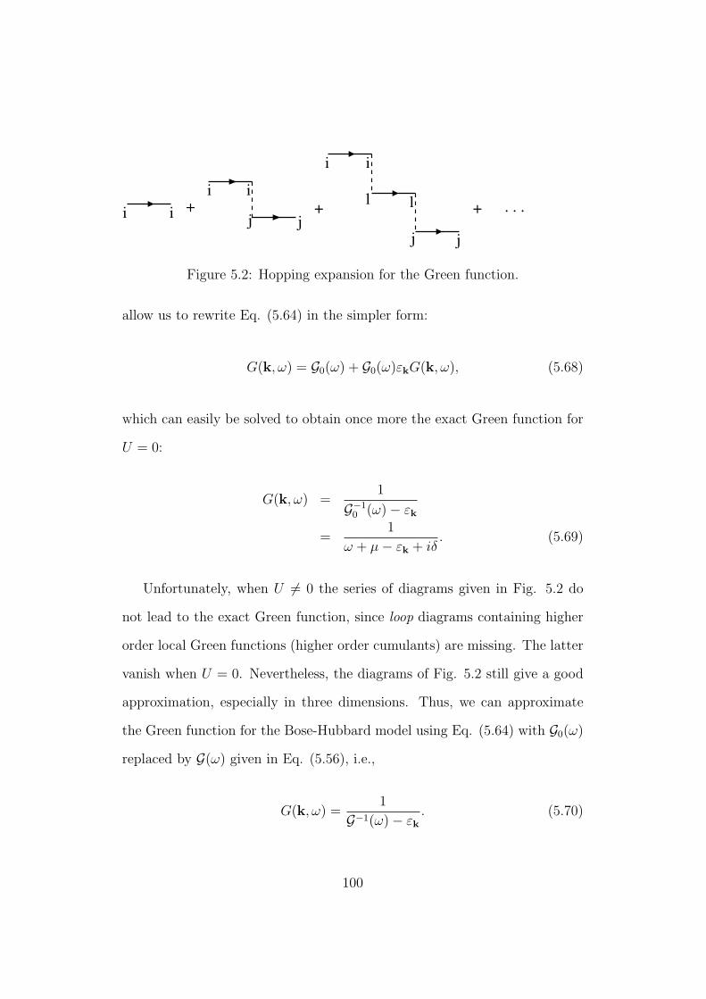
i ij j

i i

i i

l l

j j

+ + + . . .

Figure 5.2: Hopping expansion for the Green function.

allow us to rewrite Eq. (5.64) in the simpler form:

G(k, ω) = G0(ω) + G0(ω)εkG(k, ω), (5.68)

which can easily be solved to obtain once more the exact Green function for

U = 0:

G(k, ω) =1

G−10 (ω)− εk

=1

ω + µ− εk + iδ. (5.69)

Unfortunately, when U 6= 0 the series of diagrams given in Fig. 5.2 do

not lead to the exact Green function, since loop diagrams containing higher

order local Green functions (higher order cumulants) are missing. The latter

vanish when U = 0. Nevertheless, the diagrams of Fig. 5.2 still give a good

approximation, especially in three dimensions. Thus, we can approximate

the Green function for the Bose-Hubbard model using Eq. (5.64) with G0(ω)

replaced by G(ω) given in Eq. (5.56), i.e.,

G(k, ω) =1

G−1(ω)− εk. (5.70)

100

The energy spectrum is given by the poles of the above Green function:

E±(k) = −µ+1

2[εk + (2n− 1)U ]± 1

2

√ε2k + 2(2n+ 1)Uεk + U2. (5.71)

For large enough U there is an energy gap ∆ between the + and − branches

of the spectrum, which is given by

∆ = E+(0)− E−(0)

=√

(2dJ)2 − 4d(2n+ 1)UJ + U2. (5.72)

The presence of the energy gap indicates that the system is an insulator. As

U gets smaller, it will eventually attains a critical value Uc below which the

system becomes a superfluid. This critical value of U is found by demanding

that the gap vanishes for U = Uc. The condition ∆ = 0 yields

U±c = 2dJ[2n+ 1± 2

√n(n+ 1)

]. (5.73)

Note that both solutions are positive. In order to know what is the right

one we have to plot the phase diagram and study it more carefully. The

transition from the insulating phase to the superfluid phase occurs when the

bosons condense. This happens when the Green function is singular for ω = 0

and k = 0, since the bosons condense at k = 0. Thus, the phase diagram is

given by the equation

G(0) =1

εk=0

, (5.74)

101

or

n

µ/U + 1− n− n+ 1

µ/U − n=

U

2dJ. (5.75)

In Fig. 5.3 we plot the phase diagram for d = 3 and n = 1, 2, 3, 4. It

features the so called Mott lobes [67]. The phase inside the Mott lobes is

an insulating one. Outside them we have a superfluid phase. Each Mott

lobe corresponds to a Mott-insulating phase with n particles per site. Thus,

the largest lobe, corresponding to 0 ≤ µ/U ≤ 1 has n = 1. The next one,

in the interval 1 ≤ µ/U ≤ 2 has n = 2, and so on. The tips of the lobes

correspond to the points where the upper and lower bands of the spectrum

meet for k = 0, thus closing the gap. The coordinates of the tips can be

easily obtained by extremizing Eq. (5.75) with respect to µ/U . The tip of a

Mott lobe corresponds to the maximum value of J/U for a given value of n.

Extremization gives the results:

( µU

)c

=√n(n+ 1)− 1, (5.76)

Uc = 2dJ[2n+ 1 + 2

√n(n+ 1)

], (5.77)

and we see that Uc corresponds to the solution U+c of the equation ∆ = 0.

Let us compare the above results with recent highly precise Monte Carlo

(MC) simulations for the n = 1 case [74]. There it is obtained that J/Uc ≈

0.03408. On the other hand, our formula (5.77) for d = 3 and n = 1 gives

J

Uc=

1

6(3 + 2√

2)≈ 0.0286. (5.78)

102

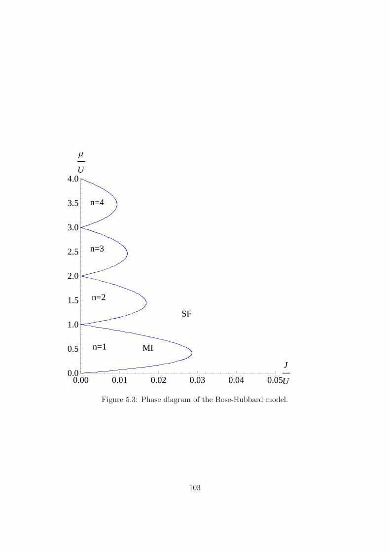
SF

MIn=1

n=2

n=3

n=4

0.00 0.01 0.02 0.03 0.04 0.05

J

U0.0

0.5

1.0

1.5

2.0

2.5

3.0

3.5

4.0

Μ

U

Figure 5.3: Phase diagram of the Bose-Hubbard model.

103

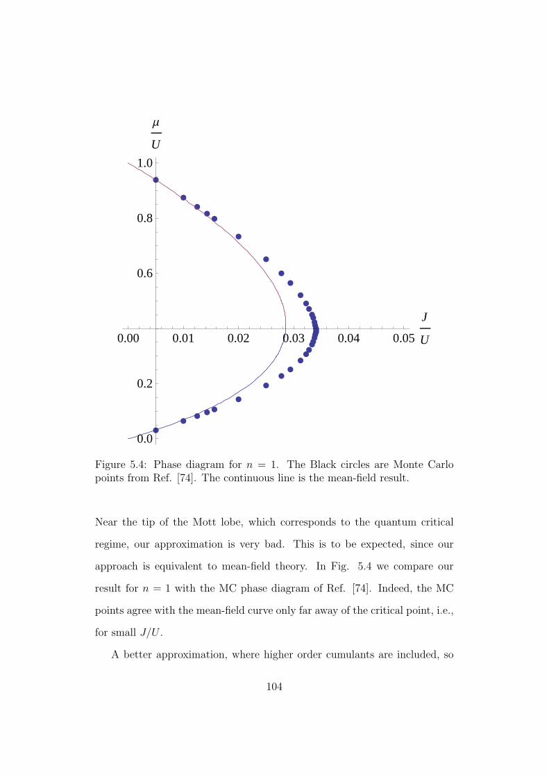
0.00 0.01 0.02 0.03 0.04 0.05

J

U

0.0

0.2

0.6

0.8

1.0

Μ

U

Figure 5.4: Phase diagram for n = 1. The Black circles are Monte Carlopoints from Ref. [74]. The continuous line is the mean-field result.

Near the tip of the Mott lobe, which corresponds to the quantum critical

regime, our approximation is very bad. This is to be expected, since our

approach is equivalent to mean-field theory. In Fig. 5.4 we compare our

result for n = 1 with the MC phase diagram of Ref. [74]. Indeed, the MC

points agree with the mean-field curve only far away of the critical point, i.e.,

for small J/U .

A better approximation, where higher order cumulants are included, so

104

that also loop diagrams appear in the hopping expansion, allows to go beyond

mean-field theory and approach better the MC result. This was done recently

in a remarkable paper by dos Santos and Pelster [75], where a quantum

Landau-Ginzburg formalism including higher order cumulants was developed.

Their result closely agrees with the MC simulations. Furthermore, in contrast

with the mean-field approach discussed here, their analysis shows how the

behavior of the phase diagram changes with the dimensionality. Their phase

diagram is shown for d = 3 in Fig. 5.5.

5.3 The Heisenberg antiferromagnet

5.3.1 Antiferromagnetic spin waves

We have seen in Chap. 2 that the spin waves in a ferromagnet have a dis-

persion ω ∼ k2. For an antiferromagnetic system the situation is different,

due to sublattice magnetization (see Fig. 5.1). Thus, in order to derive the

spin-wave excitation of a Heisenberg antiferromagnet we have to consider the

lattice sites explicitly. We will perform the calculations in the semi-classical

limit. The Heisenberg model for an antiferromagnet will be written as

H = JS2∑〈i,j〉

ni · nj, (5.79)

where n2i = 1. We can easily write down the corresponding lattice Landau-

Lifshitz equation if we rewrite the above Hamiltonian as

105

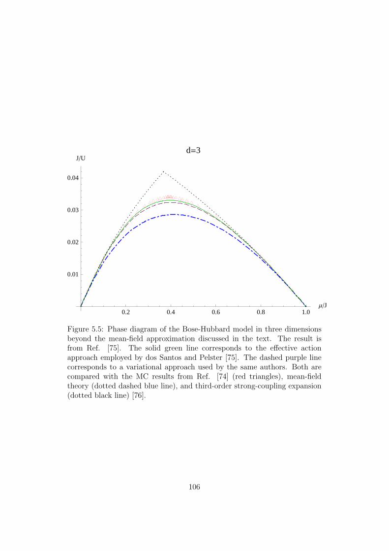
0.2 0.4 0.6 0.8 1.0Μ�J

0.01

0.02

0.03

0.04

J�Ud=3

Figure 5.5: Phase diagram of the Bose-Hubbard model in three dimensionsbeyond the mean-field approximation discussed in the text. The result isfrom Ref. [75]. The solid green line corresponds to the effective actionapproach employed by dos Santos and Pelster [75]. The dashed purple linecorresponds to a variational approach used by the same authors. Both arecompared with the MC results from Ref. [74] (red triangles), mean-fieldtheory (dotted dashed blue line), and third-order strong-coupling expansion(dotted black line) [76].

106

H = JS2∑i

ni ·Bi, (5.80)

where the effective local magnetic field is given by

Bi =′∑j

nj, (5.81)

where the prime in the sum reminds us that the sum is over the sites which

are nearest neighbors of i (that is why the effective field is i-dependent). For

example, in one dimension we have

Bi = ni−1 + ni+1. (5.82)

Therefore, the LL equation is given for the lattice model as

∂tni = JS2(ni ×Bi). (5.83)

For simplicity, we will derive the spin-wave spectrum in one dimension.

The generalization to higher dimensions is straightforward.

In one dimension the staggered magnetization occurs between even and

odd lattice sites, such that we have

n2m = n0e3 + δn⊥2m, (5.84)

and

n2m+1 = −n0e3 + δn⊥2m+1, (5.85)

107

where δn⊥i is a small transverse fluctuation that will be used to linearize the

LL equation. Thus, the calculation is similar to the one for ferromagnets in

Chap. 2, except that here we have to consider a staggered magnetization

and work on the lattice. Thus, we have the coupled equations,

∂tn2m = JS2[n2m × (n2m−1 + n2m+1)], (5.86)

∂tn2m+1 = JS2[n2m+1 × (n2m + n2(m+1))]. (5.87)

Substituting Eqs. (5.84) and (5.85) in the above equations and neglecting

terms of order higher than two in the fluctuations, we obtain,

∂tδn+2m = in0JS

2(δn+2m−1 + δn+

2m+1 + 2δn+2m), (5.88)

and

∂tδn+2m+1 = −in0JS

2(δn+2m + δn+

2(m+1) + 2δn+2m+1), (5.89)

where we have defined δn+j = δn1

j + iδn2j .

We will solve the Eqs. (5.88) and (5.89) via the Ansatze:

δn+2m = uei(2km−ωt), δn+

2m+1 = vei[(2m+1)k−ωt]. (5.90)

Thus, Eqs. (5.88) and (5.89) can be put in matrix form,

108

ω

u

v

= ω0

−1 − cos k

cos k 1

u

v

, (5.91)

where ω0 = 2n0S2J . The frequency ω is therefore determined by the eigen-

value equation,

det

−(ω + ω0) −ω0 cos k

ω0 cos k ω0 − ω

= 0, (5.92)

which yields the spin-wave spectrum:

ω(k) = ω0

√1− cos2 k = ω0| sin k|. (5.93)

The generalization to higher dimensions is straightforward, leading to the

result,

ω(k) = ω0

√√√√d2 −

(d∑a=1

cos ka

)2

. (5.94)

In the long wavelength limit, the above equation becomes

ω(k) ≈√d ω0|k|. (5.95)

Therefore, in contrast with a ferromagnet, which has a quadratic dispersion,

the antiferromagnet has a linear dispersion.

109

5.3.2 The quantum O(n) non-linear σ model

In Chap. 2 we have studied the classical O(n) non-linear σ model in de-

tail. In that Chapter the model was classical because it was being used to

describe the thermal fluctuations in a ferromagnet. However, in the context

of an antiferromagnet, the classical O(n) non-linear σ model is used to de-

scribe the quantum dynamics of an antiferromagnet at T = 0. In this case,

the temperature of the classical model studied in Chap. 2 is replaced by a

coupling constant g and the dimension d should be interpreted as D + 1,

such that d corresponds to the number of dimensions of spacetime with time

being imaginary. In this context D is the dimension of space.

The action of the quantum O(n) non-linear σ model is given by

S =1

2g

∫ β

0

dτ

∫dDx[(∂τn)2 + (∂in) · (∂in) + iλ(n2 − 1)]. (5.96)

The zero temperature case follows directly from the results for the clas-

sical model, with T replaced by g, and d being interpreted as the dimension

of spacetime. So, let us consider the so called quantum critical finite tem-

perature case. In this regime, we have that g = gc, but the temperature is

not zero, so that the mass gap m is non-vanishing. In fact, in this case the

temperature is the only energy scale available (up to the energy cutoff) and

we actually expect that m2 = aT 2, where a is a number to be determined.

For g = gc and T > 0 we still have s = 0, so that the relevant gap equation

is (2.113) (with T replaced by g), which at finite temperature becomes

110

T∞∑

n=−∞

∫dDk

(2π)D1

ω2n + k2 +m2

=1

ngc=

∫dD+1p

(2π)D+1

1

p2, (5.97)

where we have used Eq. (2.111) with T replaced by g. We stress that the

temperature T appearing in the above equation has nothing to do with the

temperature T in Chap. 2, as in the present case T arises from the integration

over τ ∈ (0, β = 1/T ) in the action.

We can perform the Matsubara sum straightforwardly (see Appendix D)

to obtain

∫dD+1p

(2π)D+1

1

p2=

∫dDk

(2π)D1

2√k2 +m2

+1

(2π)D

∫dDk√k2 +m2

1

e√k2+m2/T − 1

.

(5.98)

Note that by considering the T = 0 limit, we have from the above equation

that

∫dD+1p

(2π)D+1

1

p2=

∫dDk

(2π)D1

2|k|. (5.99)

The integrals can be easily evaluated for D = 2 and we obtain

m = −2T ln(1− e−m/T ), (5.100)

whose solution is

m(T ) = T ln

(3 +√

5

2

). (5.101)

111

The above result has been obtained before by Chubukov et al. [77].

5.3.3 The CPN−1 model

Many two-dimensional Mott insulators feature competing orders. One exam-

ple is the competition between a Neel state and a valence-bond solid (VBS)

state [79], as illustrated in Fig. 5.6. In a Landau-Ginzburg-Wilson (LGW)

framework, competing orders usually feature a first-order phase transition.

This is because the order parameters involved are the most fundamental fields

in a LGW type of theory. Furthermore, within this so called LGW paradigm

[78, 81, 82] second-order phase transitions are characterized by a very small

anomalous dimension of the order parameter. In quantum phase transitions,

on the other hand, there are examples of order parameters which are them-

selves made of more elementary building blocks. This is precisely the case of

the Neel-VBS transition illustrated in Fig. 5.6. In this case both order fields,

the staggered magnetization orientation field n and the valence-bond order

field ψVBS, are made of spinons, which in this case are more conveniently

represented as a bosonic excitation.

Mott insulators featuring competing ordered states have been matter of

intensive discussions in recent years [78]. In particular, there has been some

controversy on the nature of the Neel-VBS phase transition [83, 84, 85, 86,

87, 88]. The LGW point of view ignores the topological order of the Mott

insulator. This topological order is essential in the VBS phase, since degen-

erate VBS ground states are connected by tunneling events characterized by

a topological charge [79]. This important aspect of Mott insulators is more

112

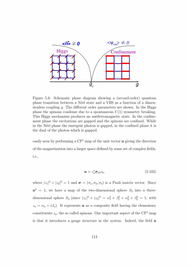
<n> 0 <ψ >VBS 0

gC

Higgs Confinement

g

Figure 5.6: Schematic phase diagram showing a (second-order) quantumphase transition between a Neel state and a VBS as a function of a dimen-sionless coupling g. The different order parameters are shown. In the Higgsphase the spinons condense due to a spontaneous U(1) symmetry breaking.This Higgs mechanism produces an antiferromagnetic state. In the confine-ment phase the excitations are gapped and the spinons are confined. Whilein the Neel phase the emergent photon is gapped, in the confined phase it isthe dual of the photon which is gapped.

easily seen by performing a CP1 map of the unit vector n giving the direction

of the magnetization into a larger space defined by some set of complex fields,

i.e.,

n = z∗aσabzb, (5.102)

where |z1|2 + |z2|2 = 1 and σ = (σ1, σ2, σ3) is a Pauli matrix vector. Since

n2 = 1, we have a map of the two-dimensional sphere S2 into a three-

dimensional sphere S3 (since |z1|2 + |z2|2 = α21 + β2

1 + α22 + β2

2 = 1, with

za = αa + iβa). It represents n as a composite field having the elementary

constituents za, the so called spinons. One important aspect of the CP1 map

is that it introduces a gauge structure in the system. Indeed, the field n

113

written in terms of spinons fields is a gauge invariant object, since the lo-

cal phase transformation za(x) → eiθ(x)za(x) leaves n invariant. This gauge

symmetry can be better understood by considering the topological charge

Q =1

8π

∮S2

dSµεµνλn · (∂νn× ∂λn), (5.103)

where Q ∈ N. We have encountered the above topological charge before in a

different context in Chap. 2, Eq. (2.31). There it was a spatial topological

object that we called a “hedgehog”, a magnetic monopole-like excitation.

The main difference between the topological charge in (5.103) and the one in

Eq. (2.31) is that the former lives in a (2 + 1)-dimensional spacetime, while

the latter arises in three-dimensional space. The spacetime hedgehog is often

called instanton.

In order to obtain the gauge field from the CP1 representation we need

the formula

εabcσaµνσ

bαβσ

cγδ = 2i(δµδδανδβγ − δµβδνγδαδ), (5.104)

which can be easily derived by using the commutation relation [σa, σb] =

2iεabcσc and the completeness relation

σaαβσaγδ = 2δαδδβγ − δαβδγδ. (5.105)

Therefore, we obtain from the CP1 map that the topological charge is given

by the magnetic flux

114

Q =1

2π

∮S2

dSµBµ, (5.106)

where Bµ = εµνλ∂νAλ and

Aµ =i

2(z∗a∂µza − za∂µz∗a). (5.107)

By coupling the above gauge field minimally to the spinons we obtain the

Lagrangian for the CP1 model

L =1

g|(∂µ − iAµ)za|2. (5.108)

In view of Eq. (5.107) and the form of the above Lagrangian together with

n = z∗aσabzb along with the corresponding constraint, it is not difficult to

see that the Lagrangian (5.108) is equivalent to the Lagrangian of the O(3)

nonlinear σ model.

The J −Q model: A lattice model for the AF-VBS transition

Competing orders need competing interactions. For instance, the AF-VBS

transition can be obtained from the following lattice model due to Sandvik

[86]:

H = J∑〈i,j〉

Si · Sj −Q∑〈ijkl〉

(Si · Sj −

1

4

)(Sk · Sl −

1

4

), (5.109)

where the sum over ijkl is around a plaquette, as shown in Fig. 5.7. The

phases of the model are as shown in Fig. 5.6. When Q/J � 1 the Heisenberg

115

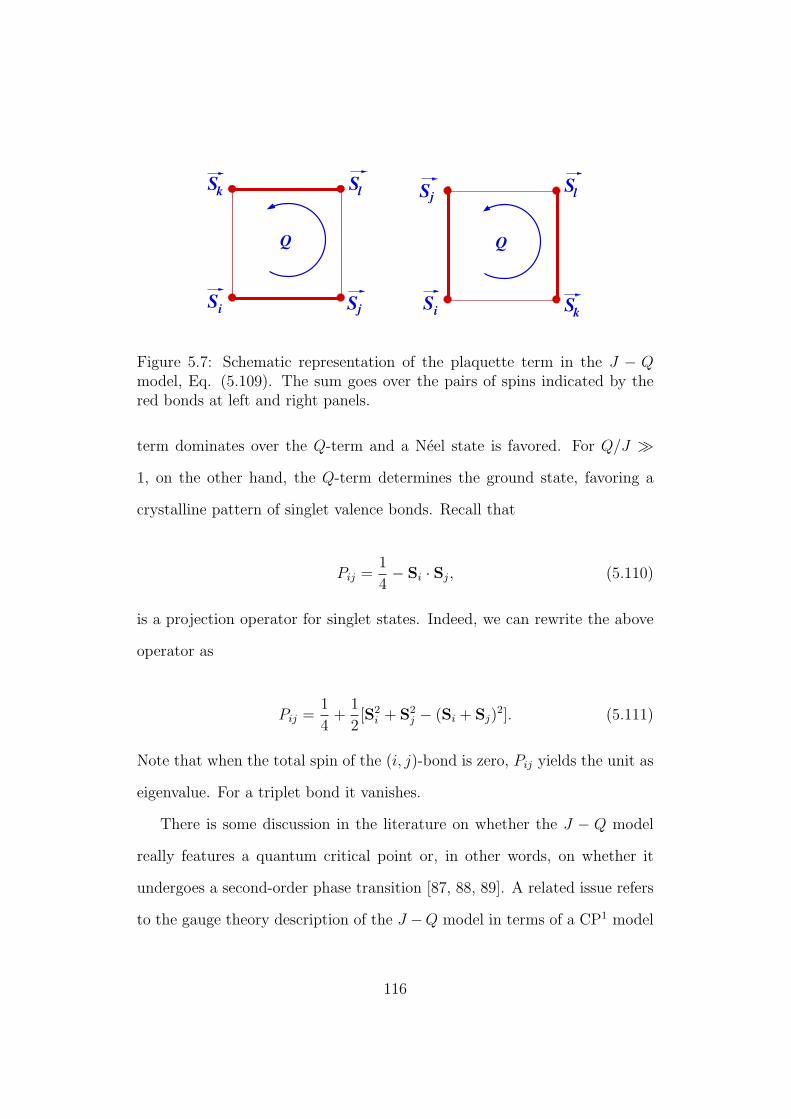
Si Sj

Sk Sl

Q

Si

Sl

Sk

Sj

Q

Figure 5.7: Schematic representation of the plaquette term in the J − Qmodel, Eq. (5.109). The sum goes over the pairs of spins indicated by thered bonds at left and right panels.

term dominates over the Q-term and a Neel state is favored. For Q/J �

1, on the other hand, the Q-term determines the ground state, favoring a

crystalline pattern of singlet valence bonds. Recall that

Pij =1

4− Si · Sj, (5.110)

is a projection operator for singlet states. Indeed, we can rewrite the above

operator as

Pij =1

4+

1

2[S2i + S2

j − (Si + Sj)2]. (5.111)

Note that when the total spin of the (i, j)-bond is zero, Pij yields the unit as

eigenvalue. For a triplet bond it vanishes.

There is some discussion in the literature on whether the J − Q model

really features a quantum critical point or, in other words, on whether it

undergoes a second-order phase transition [87, 88, 89]. A related issue refers

to the gauge theory description of the J −Q model in terms of a CP1 model

116

with instanton suppression via a Maxwell term [78, 82, 83, 84, 85]. While

Kuklov et al. [85] numerically find a weak first-order phase transition for

the CP1 model in 2 + 1 dimensions with a Maxwell term, a recent paper

by Sandvik [89] shows strong evidence that a second-order phase transition

occurs in the J − Q model. However, logarithmic violations of scaling are

also found, which may cast some doubts on whether CP1-like models can

really fully provide a description of quantum criticality in the J −Q model.

The CPN−1 model in the large N limit

The CP1 model can be generalized to include N spinons instead of two. This

yields the so called CPN−1 model, which can be studied in the large N limit.

In order to facilitate the analysis, we write the CPN−1 model as

L =1

4e20

F 2µν +

Λd−2

g

[|(∂µ − iAµ)za|2

+ iσ(|za|2 − 1)], (5.112)

such that the constraint is accounted for by the introduction of a Lagrange

multiplier field σ. Note that g here is a dimensionless coupling. We have also

introduced a Maxwell term in the Lagrangian. With this Maxwell term the

model at N = 2 is no longer equivalent to the O(3) nonlinear σ model. This

occurs only in the e0 →∞ limit. By integrating out N − 2 spinon fields we

obtain the effective action

117

Seff = (N − 2)Tr ln[−(∂µ − iAµ)2 + iσ]

+∑a=1,2

∫d3x

{1

4e20

F 2µν +

Λd−2

g

[|(∂µ − iAµ)za|2

+ iσ(|za|2 − 1)]}. (5.113)

The saddle-point equations are obtained in a standard way. We will consider

a saddle-point with Aµ = 0, iσ = σ0, and za = ζa, where σ0 and ζa are

constants. This means that no classical instanton solution is being considered

here.

The calculation below is very similar to the one made for the classical

O(n) nonlinear σ model in Chap. 2, so the reader may be interested in going

back to that Chapter again to recall the main features of the calculation.

The VBS phase occurs for g > gc, where gc is a critical coupling. In this

case we have σ0 6= 0 and ζa = 0, leading to a gap equation (for large N)

NgΛ2−d∫

ddp

(2π)d1

p2 + σ0

= 1. (5.114)

For g < gc, on the other hand, we are in the Neel phase and σ0 = 0 and

ζa 6= 0. Thus, we have

NgΛ2−d∫

ddp

(2π)d1

p2= 1−

∑a=1,2

|ζa|2. (5.115)

For g = gc we have σ0 = 0 and ζa = 0, which determines the critical coupling:

gc = (d − 2)(2π)d/(NSd), where Sd = 2πd/2/Γ(d/2) is the surface of a unit

sphere in d dimensions.

118

It is easy to see that in general we should have

∑a=1,2

|ζa|2 +g

gc− 1 = NgΛ2−dσ0

∫ddp

(2π)d1

p2(p2 + σ0). (5.116)

Therefore, we obtain for g ≥ gc,

σ0 = Λ2

[1

Γ(d/2)Γ(2− d/2)

(1− gc

g

)]2/(d−2)

. (5.117)

It is clear that σ0 should be identified with ξ−2, where ξ is the correlation

length. This leads to the well known large N critical exponent for this quan-

tity, ν = 1/(d− 2). The limit d→ 2, on the other hand, yields

σ0 = Λ2 exp

(− 4π

Ng

), (5.118)

and we see that in this case there is a gap for all g > 0.

For g < gc we obtain∑

a=1,2 |ζa|2 = 1 − g/gc, which implies that the

critical exponent of the Neel field order parameter

〈n〉 = ζ∗aσabζb (5.119)

is βN = 1. Thus, from the hyperscaling relation βN = ν(d − 2 + ηN)/2 it

follows that the anomalous dimension is

ηN = d− 2 (5.120)

for large N .

Now we consider the gauge field fluctuations to lowest order for g ≥ gc.

119

This correction is obtained from the expansion of

Tr ln[−(∂µ − iAµ)2 + σ0] (5.121)

up to quadratic order in the gauge field. In order to do this, we first note

that the covariant differential operator appearing in the inside the logarithm

can expanded as

−(∂µ − iAµ)2 = −∂2 + i∂µAµ + 2iAµ∂µ + A2, (5.122)

so that

Tr ln[−(∂µ − iAµ)2 + σ0] ≈ Tr ln(−∂2 + σ0) +G(0)

∫ddxA2(x)

− 1

2

∫ddx

∫ddx′[i∂µAµ(x) + 2iAµ(x)∂µ]G(x− x′)

× [i∂′µAµ(x′) + 2iAµ(x′)∂′µ]G(x′ − x), (5.123)

where

G(x) =

∫ddp

(2π)deip·xG(p), (5.124)

with

G(p) =1

p2 + σ0

. (5.125)

The first term on the RHS of (5.123) contributes to the saddle-point approx-

imation. The second term can be written in momentum space as

120

1

2

∫ddp

(2π)dΣµν(p)Aµ(p)Aν(−p), (5.126)

where

Σµν(p) = 2δµν

∫ddk

(2π)dG(k)−

∫ddk

(2π)d(2k − p)µ(2k − p)νG(k − p)G(k)

= 2δµν

∫ddk

(2π)d1

k2 + σ0

−∫

ddk

(2π)d(2k − p)µ(2k − p)ν

[(k − p)2 + σ0](k2 + σ0).

(5.127)

Next we set M2 = σ0 and employ some tricks of dimensional regularization.

First, by applying the operator Md/dM to both sides of Eq. (B.3) from

Appendix B, we obtain

∫ddk

(2π)d1

k2 +M2= − 2M2

d− 2

∫ddk

(2π)d1

(k2 +M2)2. (5.128)

Second, we can decompose the second integral appearing in the second line

of Eq. (5.127) into its transversal and longitudinal parts, i.e.,

∫ddk

(2π)d(2k − p)µ(2k − p)ν

[(k − p)2 +M2](k2 +M2)= Dt(p)

(δµν −

pµpνp2

)+Dl(p)

pµpνp2

.

(5.129)

By taking the trace of both sides of the above equation on one hand and

contracting with pµpν on the other hand, we can determine Dt(p) and Dl(p):

121

Dt(p) = − 1

d− 1

{4M2

d− 2

∫k

1

(k2 +M2)2

+ (p2 + 4M2)

∫k

1

[(k − p)2 +M2](k2 +M2)

},

(5.130)

and

Dl(p) = − 4M2

d− 2

∫k

1

(k2 +M2)2, (5.131)

where we have used the shorthand notation for the d-dimensional integrals

of Chap. 2, Eq. (2.37). Thus, we obtain,

Σµν(p) = −[−Dt(p) +

4M2

d− 2

∫k

1

(k2 +M2)2

]δµν

+ [Dt(p)−Dl(p)]pµpνp2

= Σ(p)

(δµν −

pµpνp2

), (5.132)

where

Σ(p) =1

d− 1

{−4M2

∫k

1

(k2 +M2)2

+ (p2 + 4M2)

∫k

1

[(k − p)2 +M2](k2 +M2)

}.

(5.133)

122

For large distances or, equivalently, in the infrared (i.e., p small), we can

write Σ(p) ≈ const p2, such that in real spacetime this fluctuation correction

generates a Maxwell term. In order to obtain this result, we have to expand

[(k − p)2 +M2]−1 up to second order in p. Thus, we have

1

(k − p)2 +M2=

1

k2 +M2+

2p · k(k2 +M2)2

+pµpν(4kµkν − δµν)

(k2 +M2)3+ . . . (5.134)

The above expression has to inserted in Eq. (5.133). In order to perform the

integrals with help of the results from Appendix B, some simplifications are

needed. First of all, rotational invariance implies

∫k

kµkν(k2 +M2)4

=δµνd

∫k

k2

(k2 +M2)4. (5.135)

Furthermore, the integral on the RHS of the above equation can be rewritten

as

∫k

k2

(k2 +M2)4=

∫k

1

(k2 +M2)3−M2

∫k

1

(k2 +M2)4. (5.136)

It should also be noted that

∫k

kµ(k2 +M2)2

= 0. (5.137)

Now we are ready to express Σ(p) in terms of the integrals evaluated in

Appendix B to obtain

123

Σ(p) =p2

d− 1

[I2(d) +

4(4− d)M2

dI3(d)− 16M4

dI4(d)

]=

p2Md−4

(d− 1)(4π)d/2

[Γ

(2− d

2

)+

2(4− d)

dΓ

(3− d

2

)− 8

3dΓ

(4− d

2

)]=

p2Md−4

3(4π)d/2Γ

(2− d

2

), (5.138)

where in the simplifications repeated use of the identity Γ(z + 1) = zΓ(z)

was made. Therefore, after replacing back M =√σ0, we obtain at large

distances the following low-energy contribution to the effective Lagrangian:

LMaxwell =1

4

(1

e20

+Ncdσ(d−4)/20

)F 2µν , (5.139)

where Fµν = ∂µAν − ∂νAµ and

cd =1

3(4π)d/2Γ

(2− d

2

). (5.140)

We have c2 = 1/(12π) and c3 = 1/(24π) for d = 2 and d = 3, respectively.

Note that even if a Maxwell term were not be present in the Lagrangian (i.e.,

e0 →∞), it would be generated by fluctuations in the paramagnetic phase.

By using M =√σ0 as a mass scale, we can define a dimensionless gauge

coupling constant f = Md−4e2, where

e2(M) =e2

0

1 + cdNe20M

d−4. (5.141)

Therefore, the RG β function for f is

124

Mdf

dM= −(4− d)f + (4− d)cdNf

2. (5.142)

Note that by expanding around d = 4 we obtain exactly the one-loop β

function for the Abelian Higgs model in the minimal subtraction scheme [5],

although we have considered N large.

We see that within the large N approach the presence of a bare Maxwell

term does not spoil the quantum critical point. Indeed, the behavior of e2

for e20 large is the same as for M small (or g → gc), provided 2 < d < 4.

However, as we have already mentioned, for the CP1 (i.e., for N = 2) model

with a Maxwell term there is strong numerical evidence against the existence

of a quantum critical point [84, 85]. However, there are indications that a

doped version of the model exhibits quantum criticality [90, 91].

Finite temperature at criticality

The finite temperature analysis at large N is similar to the one made for the

non-linear σ model, since for the leading order in 1/N we can set the gauge

field to zero. This leads again to a thermal gap

m(T ) ≡√σ0 = T ln

(3 +√

5

2

). (5.143)

Let us next calculate the uniform susceptibility χu at the QCP. In the case

of the O(3) non-linear σ model it is obtained by considering the response to

an external field twisting in the time direction of the direction field n. Thus,

the following replacement holds

125

(∂τn)2 → (∂τn− iH× n)2; (5.144)

see for example Ref. [6]. The CPN−1 model for N = 2 is equivalent to the

O(3) non-linear σ model. In this case we replace [87]

∂τza → ∂τza − iHσzabzb/2, (5.145)

for a field H = Hez. We can generalize the above to the CPN−1 model by

considering the generators of SU(N) instead of the Pauli matrices. Thus, at

leading order the large N free energy density at the presence of H becomes

for D = 2

f ≡ F/V =N

2

∞∑n=−∞

∫d2p

(2π)2[ln(ω2

n −Hωn + p2 +H2/4 +m2)

+ ln(ω2n +Hωn + p2 +H2/4 +m2)]− Λ

gcTm2. (5.146)

The uniform susceptibility is then defined by [6, 87]

χu =1

N

∂2f

∂H2

∣∣∣∣H=0

. (5.147)

Therefore,

χu =T

2

∞∑n=−∞

∫d2p

(2π)2

1

ω2n + p2 +m2

− T∞∑

n=−∞

∫d2p

(2π)2

ω2n

(ω2n + p2 +m2)2

(5.148)

126

The Matsubara sums and the integrals are straightforwardly done to obtain

χu =1

4π

[m

em/T − 1− T ln(1− e−m/T )

]. (5.149)

Upon substituting m(T ) from Eq. (5.143), we obtain

χu =T

4π

√5 ln

(1 +√

5

2

). (5.150)

5.3.4 Quantum electrodynamics in 2 + 1 dimensions

We have seen in Section 5.1 that for U � t the Hamiltonian of the Hub-

bard model becomes the Heisenberg Hamiltonian for an antiferromagnet

[Eq. (5.10)]. In this Section we will consider a generalization of it in which

the SU(2) symmetry is enlarged to SU(N). The aim of this generalization

is to provide effective field-theoretic models that can be studied systemati-

cally within a 1/N expansion. This approach was pioneered by Affleck and

Marston [92, 93] long time ago with the physical motivation of better under-

standing the Mott-insulating physics underlying the cuprates superconduc-

tors.

The SU(N) generalization of the Heisenberg model is given, up to irrel-

evant constant terms by

H = − JN

∑〈i,j〉

f †iαfjαf†jβfiβ, (5.151)

where from now on summation over repeated Greek indices is implied, J =

4t2/U [see Eq. (5.10)], and we have rescaled J → J/N in order to facili-

127

tate the large N approach. In addition, the fermions must satisfy the local

constraint:

f †iαfiα = N/2. (5.152)

By performing a Hubbard-Stratonovich transformation, we can rewrite

the Hamiltonian as

H =N

J|χij|2 −

∑〈i,j〉

χijf†iαfjα + h.c.. (5.153)

The saddle-point solution at large N is given by the so called π-flux phase,

χij = χ0eiθij ,∑

P={ijkl}

θP = π, (5.154)

corresponding to a flux amount of π around a plaquette P . This gives the

spectrum at large N :

Ek = 4χ0

√cos2 kx + cos2 ky. (5.155)

The above spectrum is gapless at the points (±π/2,±π/2).

The large N saddle-point approximation we just described corresponds

to a Mott insulator without any broken symmetries. Thus, the solution

is paramagnetic and preserves the symmetries of the square lattice. The

obtained solution constitutes one of the simplest examples of spin liquid.

128

Let us now consider the fluctuations around the saddle-point. First, we

would like to show that the elementary excitations near the nodes of the large

N spectrum (5.155) are Dirac fermions. Here we will closely follow Refs. [94]

and [95]. Let us define

χ1 = χj,j+ex , χ2 = χj+ex,j+ey ,

χ3 = χj+ex+ey ,j+ey , χ4 = χj+ey ,j. (5.156)

Since the square lattice is bipartite, we can describe it as being composed by

two interpenetrating sublattices, A and B, similarly to the mean-field theory

for the Hubbard model at half-filling discussed in Sect. 5.1. Therefore, using

Eq. (5.16), we can write

H = −∑j∈A

∑σ

(χ1c

†j+ex,σ

cjσ + χ∗4c†j+ey ,σ

cjσ + h.c.)

−∑j∈B

(χ∗3c

†j+ex,σ

cjσ + χ2c†j+ey ,σ

cjσ + h.c.)

(5.157)

+NL

J

(|χ1|2 + |χ2|2 + |χ3|2 + |χ4|2

).

Therefore, the Hamiltonian can be rewritten as

H =∑k

′[c†kσ c†kσ

] 0 |χ| (cos k1 + i cos k2)

|χ| (cos k1 − i cos k2) 0

ckσ

ckσ

,(5.158)

129

where, as before in Sect. 5.1), the prime on the sum implies that the sum is

carried over the half of the Brilouin zone. Let us denote c1kσ (c1kσ) as the

fermionic operator ckσ (ckσ) near the node (π/2, π/2). Similarly, c2kσ (c2kσ)

will denote the fermionic operator ckσ (ckσ) near the node (−π/2, π/2). Thus,

the Hamiltonian becomes approximately

H '∑k

′[c†1kσ c†1kσ c†2kσ c†2kσ

]−|χ|k1

σ1 0

0 −σ1

+|χ|k2

σ2 0

0 σ2

c1kσ

c1kσ

c2kσ

c2kσ

, (5.159)

where σ1 and σ2 are the usual Pauli matrices. The above Hamiltonian is

the one of four-component Dirac fermions in two spatial dimensions. If in

addition we include the phase fluctuations of the link field χij, i.e.,

χlm = χeiAlm , (5.160)

the Dirac fermions will get gauged. The resulting effective theory that

emerges in the continuum is quantum electrodynamics in 2 + 1 dimensions

(QED2+1), with a Lagrangian given by

Lf =N∑α=1

ψα(/∂ + ie0 /A)ψα, (5.161)

130

where we have introduced a bare “electric charge” e0 to set the energy scale,

and the standard notation /a ≡ γµaµ is used. The Dirac matrices are in this

case given by

γ0 =

σ3 0

0 −σ3

, γ1 =

σ2 0

0 −σ2

,

γ2 =

σ1 0

0 −σ1

. (5.162)

The gamma matrices above satisfy the anticommutation relation

γµγν + γνγµ = 2δµνI, (5.163)

where I is a 4× 4 identity matrix. The above relation implies

tr(γµγν) = 4δµν . (5.164)

It is well known that massless QED2+1 featuring four-component Dirac

spinors has a chiral symmetry [96], in contrast with QED2+1 involving two-

component spinors, which even admits a mass term breaking parity sym-

metry. Indeed, for the QED2+1 above there are two γ5-like matrices which

anticommute with all the other Dirac matrices, namely,

γ3 =

0 I

I 0

, γ5 =

0 I

−I 0

, (5.165)

with I being a 2×2 identity matrix. The chiral symmetry of the Lagrangian

131

(5.161) is then

ψ → eiγ3,5θψ. (5.166)

Spontaneous breaking of the chiral symmetry leads to a dynamical mass

generation in QED2+1 [98]. This mass is proportional to the chiral conden-

sate, i.e.,

m ∼N∑α=1

〈ψαψα〉. (5.167)

The dynamical mass generation implies the spontaneous breaking of the

SU(2) symmetry in the Heisenberg model, leading in this way to a stag-

gered magnetization (for more details on this point, see Ref. [99]). A similar

result [100] holds also in the case of effective QED theories for d-wave super-

conductivity [101, 102].

The dynamical mass generation in QED2+1 is more easily obtained by

studying the Schwinger-Dyson equations [98]. First of all, we need the photon

propagator in the large N limit. This is obtained in a functional integral for-

malism by performing the Gaussian integral over the Dirac fermions exactly.

In this case Dirac fields are Grassmann variables (i.e., they anticommute),

so that the effective action reads

Seff = −NTr ln(/∂ + ie0 /A). (5.168)

In order to obtain the photon propagator we simply expand the above effec-

tive action up to quadratic order in Aµ. Although we are interested in the

132

d = 3 case, we will evaluate Σµν(p) in d spacetime dimensions and set d = 3

at the end. In momentum space we obtain in this way the quadratic form,

Seff ≈1

2

∫ddp

(2π)dΣµν(p)Aµ(p)Aν(−p), (5.169)

where

Σµν(p) = −α∫

ddk

(2π)dγµG0(k)γνG0(p− k), (5.170)

with the fermionic propagator

G0(p) = − i/pp2, (5.171)

and α = Ne20. Gauge invariance implies pµΣµν(p) = 0, so that Σµν(p) is

transverse, so we can write

Σµν(p) = p2Π(p)

(δµν −

pµpνp2

). (5.172)

Taking the trace over the vector indices yields

(d− 1)p2Π(p) = α

∫ddk

(2π)dtr[γµ/kγµ(/k − /p)]

k2(p− k)2. (5.173)

Next we use the identity

γµ/pγµ = (2− d)/p, (5.174)

and the trace formula (5.164) to rewrite Eq. (5.173) as

133

(d− 1)p2Π(p) = 4(d− 2)α

∫d3k

(2π)3

k · (p− k)

k2(p− k)2. (5.175)

Since in the numerator we have

k · p− k2 =p2 − k2 − (p− k)2

2, (5.176)

and assuming the rules of dimensional regularization,2 we obtain

(d− 1)Π(p) = 2(d− 2)α

∫ddk

(2π)d1

k2(p− k)2. (5.177)

The integral in the equation above was evaluated in Chap. 2, Sect. 2.4. It

is the same as the one in Eq. (2.57), with the result of the integration given

in Eq. (2.62). Therefore,

Π(p) =2(d− 2)c(d)

d− 1|p|d−4, (5.178)

with c(d) given in Eq. (2.63). Thus, the gauge field propagator has the form

Dµν(p) =1

p2Π(p)

(δµν −

pµpνp2

), (5.179)

where Π(p) is given for d = 3 by

Π(p) =α

8|p|. (5.180)

Let us insert the propagator (5.179) in the one loop correction to the

fermionic full propagator,

2In writing the following equation we have used∫ddkk−2 =

∫ddk(p− k)−2 = 0, which

is true in dimensional regularization; see Appendix B.

134

G−1(p) = G−10 (p) +

∫d3k

(2π)3γµG(p− k)γνDµν(k), (5.181)

with a dressed fermion propagator

G(p) =1

i/pZ(p) + Σ(p)=

Σ(p)− i/pZ(p)

Z2(p)p2 + Σ2(p). (5.182)

Explicitly, we have,

i/pZ(p) + Σ(p) = i/p+8

N

∫d3k

(2π)3

γµ[Σ(k − p) + i(/k − /p)Z(k − p)]γµ[Z2(k − p)(k − p)2 + Σ2(k − p)]|k|

− 8

N

∫d3k

(2π)3

/k[Σ(k − p) + i(/k − /p)Z(k − p)]/k[Z2(k − p)(k − p)2 + Σ2(k − p)]|k|3

.(5.183)

Thus, we obtain the selfconsistent equations:

Σ(p) =16

N

∫d3k

(2π)3

Σ(k)

[Z2(k)k2 + Σ2(k)]|k + p|, (5.184)

Z(p) = 1− 8

Np2

∫d3k

(2π)3

[k2 − p2 + (k + p)2](k + p) · pZ(k)

[Z2(k)k2 + Σ2(k)]|k + p|3. (5.185)

In writing the above equations we have used the identity (5.174) and

/k/p/k = 2p · k/k − k2/p. (5.186)

After integrating over the angles, we obtain

135

Σ(p) =4

Nπ2p

∫ α

0

dkkΣ(k)(k + p− |k − p|)

Z2(k)k2 + Σ2(k)

=8

Nπ2p

[∫ p

0

dkk2Σ(k)

Z2(k)k2 + Σ2(k)+ p

∫ α

p

dkkΣ(k)

Z2(k)k2 + Σ2(k)

],

(5.187)

Z(p) = 1− 8

3π2N

[∫ α

p

dkkZ(k)

Z2(k)k2 + Σ2(k)+

1

p3

∫ p

0

dkk4Z(k)

Z2(k)k2 + Σ2(k)

].

(5.188)

From Eq. (5.187) we obtain

p2dΣ(p)

dp= − 8

Nπ2

∫ p

0

dkk2Σ(k)

Z2(k)k2 + Σ2(k), (5.189)

and therefore,

d

dp

[p2dΣ(p)

dp

]= − 8

π2N

p2Σ(p)

Z2(p)p2 + Σ2(p), (5.190)

A similar calculation using Eq. (5.188) yields

d

dp

[p4dZ(p)

dp

]=

8

π2N

p4Z(p)

Z2(p)p2 + Σ2(p). (5.191)

In Refs. [97] and [98] Z(p) is considered as being approximately one, so that

Eq. (5.191) is absent in their treatment.

From Eq. (5.187) it follows the boundary condition

136

limp→0

pΣ(p) = 0. (5.192)

Another important boundary condition is obtained from Eq. (5.187), since

pdΣ(p)

dp= −Σ(p) +

8

Nπ2

∫ α

p

dkkΣ(k)

Z2(k)k2 + Σ2(k), (5.193)

implying

pdΣ(p)

dp

∣∣∣∣p=α

= −Σ(α), (5.194)

which should be considered in addition to the boundary condition 0 ≤ Σ(0) <

∞. Similarly, from Eq. (5.188) follows the boundary condition

pdZ(p)

dp

∣∣∣∣p=α

= 3[1− Z(α)], (5.195)

while positivity of the spectral represention implies 0 < Z(0) ≤ 1.

In Ref. [96] it is found that a fermion mass is dynamically generated for

all values of N . Such a result can be obtained by considering the limit p→ 0

of Eq. (5.187) and replacing Σ(k) and Z(k) in the integrand by their lowest

order expansion in 1/N , Σ(0) and unity, respectively. Doing this we obtain

the gap equation

Σ(0) =8 Σ(0)

Nπ2

∫ α

0

dkk

k2 + Σ2(0). (5.196)

If we assume Σ(0) 6= 0 we can easily solve the above gap equation to obtain

Σ(0) = αe−Nπ2/8, (5.197)

137

reproducing the result of Ref. [96]. Under the same approximation used to

derive Eq. (5.196), we obtain from Eq. (5.188) that

Z(p) = 1 +8

3π2N

{ln

[√p2 + Σ2(0)

α

]− 1

3

+Σ2(0)

p2− Σ3(0)

p3arctan

[p

Σ(0)

]}. (5.198)

If we insert in Eq. (5.198) the trivial solution Σ(0) = 0 of the gap equation

(5.196), we obtain

Z(p) = 1 +8

3π2N

[ln( pα

)− 1

3

]. (5.199)

The above equation implies the existence of an anomalous dimension η de-

fined through

η = − limp→0

pd lnZ(p)

dp, (5.200)

and we obtain the known 1/N result [103]

η = − 8

3π2N. (5.201)

On the other hand, the p→ 0 limit gives

Z(0) = 1 +8

3π2Nln

[Σ(0)

α

]. (5.202)

Substitution of the result (5.197) in (5.202) yields Z(0) = 2/3, which con-

tradicts the value Z(0) = 3/4 obtained in Ref. [96] through an argument

138

involving the Ward identities 3. The contradiction is removed if instead of

Eq. (5.196) the following gap equation is used:

Σ(0) =8 Σ(0)

Nπ2

∫ α

0

dkk

Z2(0)k2 + Σ2(0). (5.203)

In this case we obtain

Σ(0) = αZ(0)e−Nπ2Z2(0)/8, (5.204)

Z(0) = 1 +8

3π2NZ(0)ln

[Σ(0)

αZ(0)

], (5.205)

implying that

Z(0) =3

4. (5.206)

Note that such a modification affects the value of the anomalous dimension,

since in the limit of a vanishing gap we have

Z(p) = 1 +8

3π2NZ(0)

[ln( pα

)− 1

3

]= 1 +

32

9π2N

[ln( pα

)− 1

3

], (5.207)

instead of the standard 1/N result (5.199). Thus, we obtain instead of Eq.

(5.201) the result

η = − 32

9π2N. (5.208)

Thus, revisiting the earlier approach of Ref. [96] taught us an impor-

tant lesson: in order to not violate the Ward identities when linearizing the

3This result is discussed in Ref. [19] of Ref. [96].

139

problem, we have to account not only for Σ(0) but also for Z(0).

We consider next an improved linearized problem given by the approxi-

mated differential equations

d

dp

[p2dΣ(p)

dp

]= − 8

π2N

p2Σ(p)

Z2(0)p2 + Σ2(0), (5.209)

d

dp

[p4dZ(p)

dp

]=

8

π2N

p4Z(p)

Z2(0)p2 + Σ2(0). (5.210)

The solutions obeying the initial conditions Σ′(0) = 0 and Z ′(0) = 0, while

Σ(0) 6= 0 and Z(0) 6= 0, as required by the boundary conditions, are

Z(p) = Z(0)2F1

[3

4− 3

4ζ,

3

4+

3

4ζ;

5

2;−Z

2(0)p2

Σ2(0)

], (5.211)

Σ(p) = Σ(0)2F1

[1

4− i

4γ,

1

4+

i

4γ;

3

2;−Z

2(0)p2

Σ2(0)

], (5.212)

where 2F1 is a hypergeometric function and

ζ =

√1 +

32

9π2Z2(0)N, γ =

√32

π2Z2(0)N− 1. (5.213)

The solution (5.212) with Z(0) = 1 was obtained before in Ref. [104].

The CSB is more easily analysed in the regime where Z2(0)p2 � Σ2(0),

in which case the above solutions simplify to

Z(p) ≈ 9√π

8Z(0)B

[Z(0)p

Σ(0)

]−3/2

cosh

{3ζ

2ln

[Z(0)p

Σ(0)

]+ ϕ

}, (5.214)

Σ(p) ≈ |C|4

√πΣ3(0)

Z(0)pcos

{γ

2ln

[Z(0)p

Σ(0)

]+ θ

}, (5.215)

140

where

A± =Γ(±ζ)(1± ζ)

Γ2(

74± 3ζ

4

) , B =√|A+A−|, C =

Γ(iγ/2)(1 + iγ)

Γ2(

54

+ iγ4

) ,

(5.216)

and

θ = arccos

(C + C∗

2|C|

), ϕ =

1

2ln

∣∣∣∣A+

A−

∣∣∣∣ . (5.217)

The boundary conditions can be used to determine Σ(0) and simplify the

above equations. For Σ(0) we obtain

Σ(0) = αZ(0) exp

{−2

γarccos

[πZ(0)

4

√N

2(sin θ + γ cos θ)

]}. (5.218)

Note that the critical number of flavors is now modified due to the wave

function renormalization at p = 0 and given by demanding that γ vanishes,

i.e.,

Nch =32

π2Z2(0). (5.219)

Therefore, Eq. (5.218) can be rewritten as

Σ(0) = αZ(0) exp

{−2

γarccos

[√N

Nch

(sin θ + γ cos θ)

]}. (5.220)

Note that θ is non-singular as N → Nch, approaching the value (2m+ 1)π/2,

with m = 1, 2, . . . . Thus, near N = Nch Eq. (5.220) becomes

Σ(0) = αZ(0) exp

(−2πn

γ

), (5.221)

with n = 1, 2, . . . , which agrees with Ref. [98] for Z(0) = 1. Interestingly,

141

the functional form of the generated mass gap Σ(0) resembles the one in Eq.

(3.63) for the KT transition. In the present case the number of fermionic

degrees of freedom is playing the role of the temperature.

Inserting (5.221) with n = 1 in (5.214) yields

Z(p) =9√π

8Z(0)Be−3π/γ

( pα

)−3/2

cosh

[3ζ

2ln( pα

)+

3πζ

γ+ ϕ

]. (5.222)

Using Eq. (5.195) this can be further rewritten as

Z(p) =2(p/α)−3/2

cosh(3πζ/γ + ϕ) + ζ sinh(3πζ/γ + ϕ)cosh

[3ζ

2ln( pα

)+

3πζ

γ+ ϕ

].

(5.223)

For N ≥ Nch the mass gap Σ(0) vanishes and the above equation becomes

simply

Z(p) =2

1 + ζ

( pα

)−eη, (5.224)

which defines the anomalous dimension

η =3

2(1− ζ). (5.225)

Precisely at N = Nch we have η = −0.08. On the other hand, for N � Nch

we obtain the following large N result:

η ≈ − Nch

12N= − 8

3π2Z2(0)N. (5.226)

The result (5.225) can be more easily obtained by considering Eq. (5.191)

142

at the critical point, in which case it becomes

d

dp

[p4dZ(p)

dp

]=

8

π2N

p2

Z(p). (5.227)

Eq. (5.227) can be rewritten as a set of two RG-like equations:

pd lnZ(p)

dp= −γ(p), (5.228)

pdγ

dp= γ(γ − 3)− 8

π2NZ2. (5.229)

Thus, η = limp→0 γ(p). This limit is attained at the fixed point, which in

this case is given by

γ± =3

2(1± ζ). (5.230)

Only the solution γ− makes sense since γ+ > 3, which would lead to a

vanishing of the fermion propagator as p → 0. Therefore, we obtain that

η = γ−, in agreement with Eq. (5.225).

Within the present calculation the determination of Z(0) is not so straight-

forward, as the approximation we have used implies an anomalous dimension.

On the other hand, since the anomalous dimension arises only for vanishing

gap, it is reasonable to assume that η coincides with the anomalous dimen-

sion we have computed before, Eq. (5.208). Thus, we demand that η = η,

such that Z(0) =√

3/2 is obtained, contrasting with the Z(0) obtained be-

fore, which is given by the square of the present result. Therefore, we obtain

from Eq. (5.219) the critical value Nch = 128/(3π2) ≈ 4.32, in full agreement

with the result of Ref. [105] and the one of Ref. [106] in the case where the

143

anomalous dimension is computed up to order 1/N .

The physical interpretation of the above results is as follows. The num-

ber Nch separates two different insulating regimes, namely, a magnetically

ordered one at N < Nch and another one having no broken symmetries

at N > Nch. The latter can be identified with a U(1) spin liquid state.

The physically interesting case is N = 2, which corresponds to an SU(2)

Heisenberg antiferromagnet. Thus, the above Schwinger-Dyson calculation

indicates that there is no spin liquid state in this case. However, there is

numerical evidence [107] that the Schwinger-Dyson approach overestimates

the value of Nch. The numerical analysis made in Ref. [107] indicates that

Nch ≈ 1.5. This result is in agreement with an earlier prediction [108] based

on mathematical inequalities and symmetry arguments. If this result is cor-

rect, it would imply that the two-dimensional Heisenberg antiferromagnet

has a spin liquid ground state.

144

Acknowledgements

I would like to the thank the organizers of the VIII School of Physics of the

CBPF (Brazilian Center for Research in Physics in the Portuguese abrevia-

tion), especially the director of the school, Luiz Sampaio, and the colleagues

who helped to make the invitation possible, like Adolfo P. C. Malbouisson

and Itzhak Roditi, with whom I had many interesting discussions during my

stay.

I have discussed with several colleagues on the topics of these lecture notes

in the last years. I would like to thank in particular my collaborators Hagen

Kleinert, Asle Sudbø, Karl Bennemann, Ilya Eremin, Rene Tarento, Zohar

Nussinov, Dirk Manske, Steinar Kragset, Joakim Hove, Eivind Smørgrav,

and Jo Smiseth.

I had many illuminating discussions with the following colleagues. For the

topic on quantum phase transitions in Mott insulators, I benefited in the last

years from discussions I had with Anders Sandvik, Subir Sachdev, Anatoly

Kuklov, Nikolay Prokof’ev, Boris Svistunov, Zi Cai, and Ying Jiang. For top-

ics around QED in 2 + 1 dimensions I had many interesting discussions with

Igor Herbut, Zlatko Tesanovic, Jorg Schmalian, Guo-Zhu Liu, Petr Jizba, and

Jurgen Dietel. I also benefited from discussions I had on Bose-Einstein con-

145

densation with Axel Pelster, Anna Posazhennikova, Adriaan Schakel, Victor

Bezerra, Ednilson Santos, and Aristeu Lima.

146

Appendices

147

Appendix A

The surface of a sphere in d

dimensions

In this appendix we will derive the formula for the surface of a sphere whose

radius is unity in d dimensions. Such a factor occurs in many calculations in

the text and we will derive it here as a simple exercise involving d-dimensional

integrals. The trick is to consider the d-dimensional Gauss integral

I =

∫ddxe−x2

(A.1)

in two ways. In the first way we simply evaluate the above integral directly,

since it is just an ordinary one-dimensional Gauss integral to the power d.

Thus,

I = πd/2. (A.2)

148

Next, we use spherical coordinates in d dimensions and formally perform

the integral over the d − 1 angular variables. We call the result of such an

integration Sd, which is precisely the surface of a unit sphere in d dimensions.

In this way, we can also write,

I = Sd

∫ ∞0

drrd−1e−r2

. (A.3)

Now we make the change of variables u = r2, such that,

I =Sd2

∫ ∞0

duud/2−1e−u

=SdΓ(d/2)

2, (A.4)

where we have used the definition of the gamma function. From Eq. (A.2)

we obtain immediately,

Sd =2πd/2

Γ(d/2), (A.5)

which is the desired result.

149

Appendix B

Dimensional regularization and

evaluation of some simple

integrals in d dimensions

In this Appendix we evaluate the following simple d-dimensional integrals

and, at the same time, introduce the method of dimensional regularization

of integrals:

I1 =

∫ddk

(2π)d1

k2 +M2, (B.1)

and

I2 =

∫ddk

(2π)d1

(k2 +M2)2. (B.2)

Both integrals can be obviously be done in 2 < d ≤ 4 if an ultraviolet cutoff

Λ is introduced. In the limit Λ → ∞ divergencies appear. Dimensional

150

regularization converts logarithmic divergencies due to the infinite cutoff into

poles for some values of d. Moreover, divergencies involving positive powers

of Λ “disappear”. In order to understand the consistence of the technique, let

us consider the integral I1 as a function of M and d, while demanding that it

should be cutoff independent. This can be done by considering d somewhere

in the complex plane, such that the integral is convergent. The result of

the integration, as a function of d, can then be analytically continued in a

larger domain (for more details, see Refs. [5] and [8]). In this way, simple

dimensional analysis yields

I1(M,d) = c1(d)Md−2, (B.3)

where c(d) is a dimensionless function of d. We obtain similarly for I2,

I2(M,d) = c2(d)Md−4. (B.4)

Note that if it is assumed that no cutoff is needed, the only scale available

is M . This way of doing things is not always useful and sometimes we may

need the explicit cutoff dependence. Note that Eq. (B.3) implies that I1

vanishes for all d > 2 if M = 0, which is certainly not true if we regularize

the integral with a cutoff. Indeed, if a cutoff is introduced, we have

I1(0, d) =SdΛ

d−2

d− 2, (B.5)

thus leading to a positive power of Λ when d > 2. Thus, by demanding that

I1(M,d) is independent of Λ for all d, we obtain that this condition actually

151

imposes

∫ddk

(2π)d1

k2= 0. (B.6)

The above equation is one of the properties required by dimensional regular-

ization. In fact, an even more general formula should be used, namely,

∫ddk

(2π)d1

kα= 0, (B.7)

where α ∈ C.

We now proceed with the explicit evaluation of the constants c1(d) and

c2(d). To this end, note that the integral I1 can be written as

I1 =

∫ ∞0

dλ

∫ddk

(2π)de−λ(k2+M2). (B.8)

The d-dimensional Gauss integral is easily performed to obtain,

I1 =1

(4π)d/2

∫ ∞0

dλλ−d/2e−λM2

. (B.9)

By changing the variable as u = M2λ, we obtain,

I1 =Md−2

(4π)d/2

∫ ∞0

duu−d/2e−u =Md−2

(4π)d/2Γ

(1− d

2

), (B.10)

where we have used the integral definition of the gamma function.

The integral I2 is obtained from I1 via simple differentiation of I1 with

respect to M2. We obtain,

152

I2 = − ∂I1

∂M2=

Md−4

(4π)d/2Γ

(2− d

2

). (B.11)

Note that the integral I1 has poles for d = 2 and for d = 4, while I2 has

only a pole at d = 4.

Now we will consider the most general case, i.e., we will evaluate the

integral

Iα(d) =

∫ddk

(2π)d1

(k2 +M2)α. (B.12)

Using the identity (2.43), we have,

Iα(d) =1

Γ(α)

∫ ∞0

dλ

∫ddk

(2π)de−λ(k2+M2)λα−1

=1

(4π)d/2Γ(α)

∫ ∞0

dλλα−1−d/2e−λM2

=Md−2α

(4π)d/2Γ(α)

∫ ∞0

duuα−1−d/2e−u

=Md−2α

(4π)d/2Γ(α)Γ

(α− d

2

), (B.13)

where from the first to the second line we have performed the d-dimensional

Gauss integral in k and from the second to the third line we made the sub-

stitution u = M2λ. From the third to the last line we used the definition of

the gamma function.

Of course, for α = 1 and α = 2 the integral (B.13) reproduces the results

I1 and I2, respectively.

153

Appendix C

Evaluation of the integral over

a Bose-Einstein distribution in

d dimensions

Let us consider the following integral:

IBE(z,D) =

∫ddk

(2π)d1

ec|k|z − 1

=Sd

(2π)d

∫ ∞0

dkkd−1

eckz − 1, (C.1)

where c > 0 and Sd is given in Appendix A. The exponent z > 0 defines the

power law for the spectrum of the corresponding Bose particle. For example,

a free particle will have z = 2, while phonons have z = 1.

After performing the change of variables u = ckz, the integral becomes,

154

IBE(z,D) =Sd

(2π)dzcd/z

∫ ∞0

ud/z−1

eu − 1. (C.2)

In order to calculate the integral appearing in the expression above, we con-

sider the integral representation of the gamma function,

Γ(s) =

∫ ∞0

dtts−1e−t, (C.3)

and make the replacement t → nt, where n is a positive integer. This leads

to

Γ(s)

ns=

∫ ∞0

dtts−1e−nt. (C.4)

Now we sum over n from 1 to ∞,

Γ(s)∞∑n=1

1

ns=

∫ ∞0

dtts−1

∞∑n=1

e−nt. (C.5)

On the LHS of the above equation appears the definition of the zeta function,

ζ(s) =∞∑n=1

1

ns, (C.6)

while on the RHS features a trivial geometric sum,

∞∑n=1

e−nt =1

1− e−t− 1 =

1

et − 1. (C.7)

Therefore,

ζ(s)Γ(s) =

∫ ∞0

dtts−1

et − 1. (C.8)

155

Using the above result in Eq. (C.2), we obtain finally,

IBE(z,D) =Sd

(2π)dzcd/zζ

(d

z

)Γ

(d

z

). (C.9)

156

Appendix D

Matsubara sums

The computation of Matsubara sums is a standard method in both relativistic

and non-relativistic quantum field theory; see for example Ref. [109].

Let us evaluate here two bosonic Matsubara sums frequently used in the

text, namaly,

S1 = − 1

β

∞∑n=−∞

1

iωn − ε, (D.1)

and

S2 =1

β

∞∑n=−∞

1

ω2n + ε2

, (D.2)

where ωn = 2πn/β.

Although, strictly speaking, the first sum does not converge, it can nev-

ertheless be done using regularization methods. Moreover, as we will see, it

is related to the second sum, which is convergent.

Since S2 is convergent, let us calculate this one first.

157

������������

������������

�������������

�������������

����

���������������������������������������������������������

���������������������������������������������������������

���������������������������������������������������������

���������������������������������������������������������

C2

C1

εε

������

������

������

������

Figure D.1: Initial contour integration in complex plane used for performingthe Matsubara sum S2. The red crosses indicate the position of the Matsub-ara modes.

In order to calculate S2, we rewrite the sum in terms of a contour integral

over an appropriate contour in such a way as to set the sum of the residues

at poles given by the Matsubara frequency modes. The two straight lines

shown in Fig. D.1 enclose all Matsubara modes. We can imagine a finite

number of modes with a closed curve around all of them. In the limit of

an infinite number of modes, the closed curve becomes two parallel lines

having the Matsubara modes between them. This picture explains why the

arrows are pointing the way they do: if to the closed curve a counterclockwise

orientation is given, in the limit of an infinite number of Matsubara modes

the resulting straight line on the right will point upwards, while the one on

the left will point downwards. Thus, the sum S2 is equivalent to

158

����

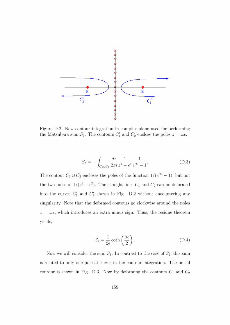
C1

C2

εε

������

������

������

������

Figure D.2: New contour integration in complex plane used for performingthe Matsubara sum S2. The contours C ′1 and C ′2 enclose the poles z = ±ε.

S2 = −∫C1∪C2

dz

2πi

1

z2 − ε21

eβz − 1. (D.3)

The contour C1 ∪ C2 encloses the poles of the function 1/(eβz − 1), but not

the two poles of 1/(z2 − ε2). The straight lines C1 and C2 can be deformed

into the curves C ′1 and C ′2 shown in Fig. D.2 without encountering any

singularity. Note that the deformed contours go clockwise around the poles

z = ±ε, which introduces an extra minus sign. Thus, the residue theorem

yields,

S2 =1

2εcoth

(βε

2

). (D.4)

Now we will consider the sum S1. In contrast to the case of S2, this sum

is related to only one pole at z = ε in the contour integration. The initial

contour is shown in Fig. D.3. Now by deforming the contours C1 and C2

159

������������

������������

�������������

�������������

���������������������������������������������������������

���������������������������������������������������������

���������������������������������������������������������

���������������������������������������������������������

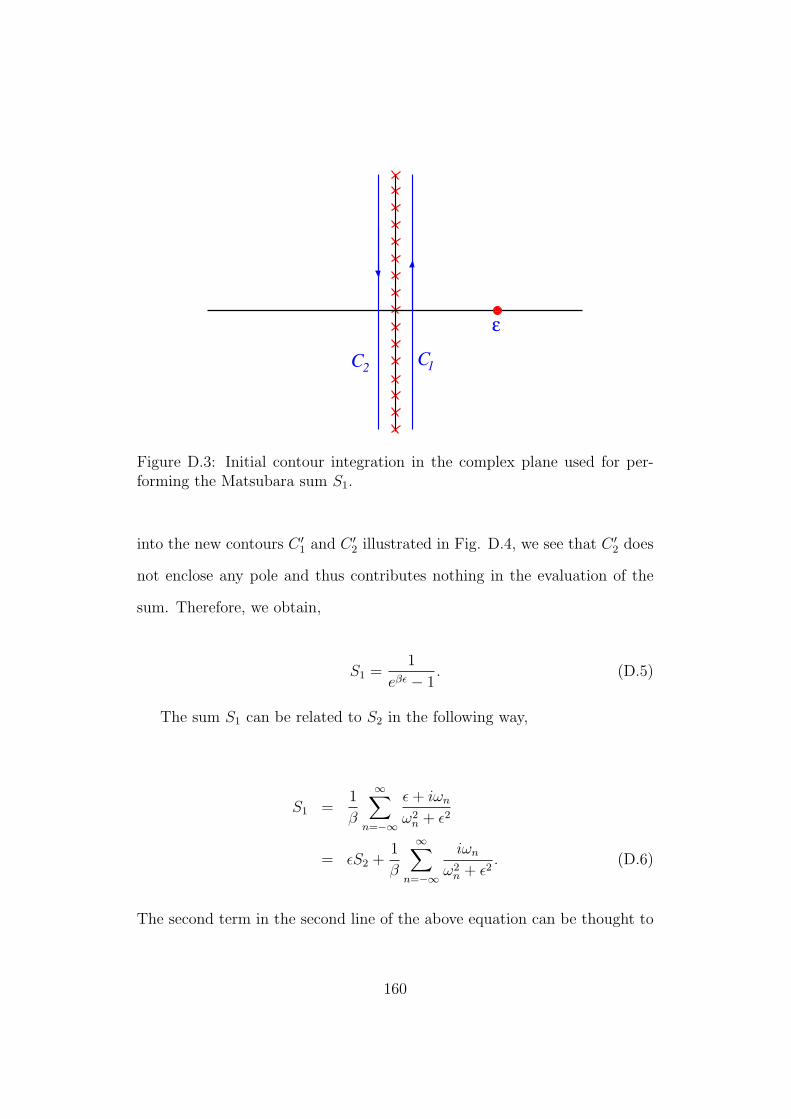
C2

C1

ε

������

������

Figure D.3: Initial contour integration in the complex plane used for per-forming the Matsubara sum S1.

into the new contours C ′1 and C ′2 illustrated in Fig. D.4, we see that C ′2 does

not enclose any pole and thus contributes nothing in the evaluation of the

sum. Therefore, we obtain,

S1 =1

eβε − 1. (D.5)

The sum S1 can be related to S2 in the following way,

S1 =1

β

∞∑n=−∞

ε+ iωnω2n + ε2

= εS2 +1

β

∞∑n=−∞

iωnω2n + ε2

. (D.6)

The second term in the second line of the above equation can be thought to

160

vanish, as to every positive term there is a corresponding negative term of

identical magnitude. Thus, it seems that we just have to plug the result of

the sum S2 into the above result and we are done. However, this is not quite

correct. The point is that S2 involves two poles, z = ±ε, corresponding to a

“particle” and an “anti-particle” mode, while S1 involves just a single pole

at z = ε. Actually the second sum in Eq. (D.6) is not convergent. This is

consistent with the the already mentioned fact, that the sum (D.1) is not

convergent. Since,

S1 =1

2coth

(βε

2

)+ S3 =

1

2+

1

eβε − 1+ S3, (D.7)

where

S3 =1

β

∞∑n=−∞

iωnω2n + ε2

, (D.8)

and using Eq. (D.5), we obtain that

S3 = −1

2. (D.9)

The factor 1/2 subtracted via the sum S3 reflects the “vacuum” con-

tribution associated to the particle-antiparticle pair. In S2 this leads to a

finite zero-temperature contribution, which is absent in the non-relativistic

Matsubara sum.

161

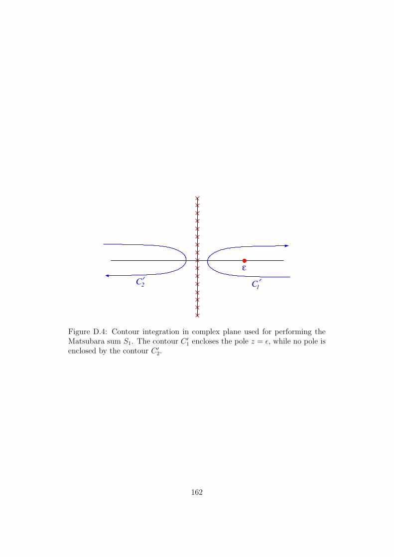
C1

C2

ε

������

������

Figure D.4: Contour integration in complex plane used for performing theMatsubara sum S1. The contour C ′1 encloses the pole z = ε, while no pole isenclosed by the contour C ′2.

162

Appendix E

Classical limit of the

polarization bubble of the

dilute Bose gas

After setting λ0 = µ Eq. (4.44) can be rewritten as

Π(iω,p) = 4m2

∫ddq

(2π)dnB

(q2

2m

)(1

2miω − p2 − 2p · q− 1

2miω + p2 − 2p · q

).

(E.1)

In the classical approximation we write nb(x) ≈ T/x and the polarization

bubble can be rewritten as

Π(iω,p) = 4m2T (I+ − I−), (E.2)

where

163

I± = −i∫

ddq

(2π)d1

2mω + i(2p · q± p2)

1

q2. (E.3)

The integrals I± can be evaluated using the Feynman parameters [8],

I± = −i∫ ∞

0

dλ1

∫ ∞0

dλ2ddq

(2π)de−λ1(2mω±ip2+2ip·q)e−λ2q2 . (E.4)

After evaluating the Gaussian integral over q we obtain

I± = − i

(2π)d

∫ ∞0

dλ1

∫ ∞0

dλ2

(π

λ2

)d/2e−λ1(2mω±ip2)e−p

2λ21/λ2

= ∓(±i)d−2

2dπd/2Γ(d/2− 1)Γ(3− d)pd−4

(1∓ 2miω

p2

)d−3

. (E.5)

Substituting the above expression back into (E.2) we obtain Eq. (4.61).

164

Bibliography

[1] K. G. Wilson and J. B. Kogut, Physics Reports 12C, 76 (1974).

[2] H. Kleinert, Gauge Fields in Condensed Matter, Vols. 1 and 2 (World

Scientific, Singapore, 1989).

[3] E. Fradkin, Field Theories of Condensed Matter Systems (Addison-

Wesley, 1991).

[4] D. I. Uzunov, Introduction to the Theory of Critical Phenomena (World

Scientific, Singapore, 1992).

[5] J. Zinn-Justin, Quantum Field Theory and Critical Phenomena, 2nd

ed. (Oxford University Press, Oxford, 1993).

[6] S. Sachdev, Quantum Phase Transitions (Cambridge University Press,

1999).

[7] N. Nagaosa, Quantum field theory in condensed matter physics

(Springer, Berlin, 1999).

[8] H. Kleinert and V. Schulte-Frohlinde, Critical properties of ϕ4-theory

(World Scientific, Singapore, 2001).

165

[9] M. Continentino, Quantum scaling in many-body systems (World Sci-

entific, Singapore, 2001).

[10] X.-G. Wen, Quantum Field Theory of Many-Body Systems (Oxford

University Press, 2004).

[11] I. F. Herbut, A modern approach to critical phenomena (Cambridge

University Press, 2007).

[12] A. M. J. Schakel, Boulevard of Broken Symmetries: Effective Field

Theories of Condensed Matter (World Scientific, Singapore, 2009).

[13] J. B. Kogut, Rev. Mod. Phys. 51, 659 (1979).

[14] P. A. Lee., N. Nagaosa, and X.-G. Wen, Rev. Mod. Phys. 78,17 (2006).

[15] L. D. Landau and E. M. Lifshitz, Statistical Mechanics, Part I, 3rd

edition revised and enlarged by E. M. Lifshitz and L. P. Pitaevskii

(Pergamon Press, 1980).

[16] V. Rivasseau, From perturbative to constructive renormalization

(Princeton University Press, Princeton, NJ, 1994).

[17] D. J. Amit and G. B. Kotliar, Nucl. Phys. B 170, 187 (1980).

[18] A. McKane and M. Stone, Nucl. Phys. B 163, 169 (1980).

[19] P.C. Hohenberg, Phys. Rev. 158, 383 (1967).

[20] N.D. Mermin and H. Wagner, Phys. Rev. Lett. 17, 1133 (1966).

[21] J. M. Kosterlitz and D. J. Thouless, J. Phys. C 6, 1181 (1973).

166

[22] H. Kleinert, Multivalued Fields in Condensed Matter, Electromag-

netism, and Gravitation (World Scientific, Singapore, 2008).

[23] J. M. Kosterlitz, J. Phys. C 7, 1046 (1974).

[24] D. R. Nelson and J. M. Kosterlitz, Phys. Rev. Lett., 39, 1201 (1977).

[25] G. Agnolet, D.F. McQueeney, and J.D. Reppy, Phys. Rev. B 39, 8934

(1989).

[26] J.M. Kosterlitz, J. Phys. C 10, 3753 (1977).

[27] P. W. Anderson, J. Phys. C: Solid State Phys. 3, 2436 (1970).

[28] H. Kleinert, F.S. Nogueira, and A. Sudbø, Nucl. Phys. B 666, 361

(2003).

[29] F. S. Nogueira and H. Kleinert, Phys. Rev. B 77, 045107 (2008).

[30] A. P. Young, Phys. Rev. B19, 1855 (1982).

[31] J. Frohlich and T. Spencer, J. Stat. Phys. 24, 617 (1981).

[32] A. M. Polyakov, Nucl. Phys. B 120, 429 (1977).

[33] L. B. Ioffe and A. I. Larkin, Phys. Rev. B 39, 8988 (1989).

[34] H. Kleinert, F.S. Nogueira, and A. Sudbø, Phys. Rev. Lett. 88, 232001

(2002).

[35] I.F. Herbut and B.H. Seradjeh, Phys. Rev. Lett. 91, 171601 (2003).

[36] I.F. Herbut, B.H. Seradjeh, S. Sachdev, and G. Murthy, Phys. Rev. B

68, 195110 (2003).

167

[37] S. Kragset, A. Sudbø, and F. S. Nogueira, Phys. Rev. Lett. 92, 186403

(2004).

[38] K. Borkje, S. Kragset, and A. Sudbø, Phys. Rev. B 71, 085112 (2005).

[39] M. Hermele, T. Senthil, M.P.A. Fisher, P.A. Lee, N. Nagaosa, and

X.-G. Wen, Phys. Rev. B 70, 214437 (2004).

[40] F.S. Nogueira and H. Kleinert, Phys. Rev. Lett. 95, 176406 (2005).

[41] F. S. Nogueira and Z. Nussinov, Phys. Rev. B 80, 104413 (2009).

[42] P.C. Hohenberg and P.C. Martin, Ann. Phys. (N.Y.) 34, 291 (1965).

[43] F. S. Nogueira, in W. Janke and A. Pelster (Editors): Proceedings

of the 9th International Conference Path Integrals – New Trends and

Perspectives (World Scientific, Singapore, 2007).

[44] J. O. Andersen, Rev. Mod. Phys. 76, 599 (2004).

[45] L. Pitaevskii and S. Stringari, J. Low Temp. Phys. 85, 377 (1991).

[46] F. S. Nogueira and H. Kleinert, Phys. Rev. B 73, 104515 (2006).

[47] A. A. Abrikosov, L.P. Gorkov, and I.E. Dzyaloshinski, Methods of

Quantum Field Theory in Statistical Physics (Dover Publications, Inc.,

1975).

[48] N.N. Bogoliubov, Izv. Akad. Nauk SSSR, Ser. Fiz. 11, 77 (1947) [Engl.

transl. J. Phys. (U.S.S.R.) 11, 23 (1947)].

168

[49] Yu. A. Tserkovnikov, Dokl. Akad. Nauk SSSR 159, 1023 (1964) [Engl.

trans.: Soviet Phys. Dokl. 9, 1095 (1965)].

[50] I. Kondor and P. Szepfalusy, Phys. Lett. A 33, 311 (1970).

[51] T. H. Cheung and A. Griffin, Canad. J. Phys. 48, 2135 (1970); Phys.

Lett. A 35, 141 (1971).

[52] P. Szepfalusy and I. Kondor, Ann. Phys. (N.Y.) 82, 1 (1974).

[53] I. Kondor and P. Szepfalusy, Phys. Lett. A 47, 393 (1974).

[54] P. Szepfalusy and I. Kondor, in: Proceedings of the International School

of Physics “Enrico Fermi”: Local Properties of Phase transitions, K.A.

Muller (Ed.) (North-Holland, Amsterdam, 1976), p. 806.

[55] R. Abe, Prog. Theor. Phys. 52, 1135 (1974); R. Abe and Hikami, Prog.

Theor. Phys. 52, 1463 (1974).

[56] A.Z. Patashinskii and V.L. Pokrovskii, Soviet Phys. JETP 19, 677

(1964).

[57] R.A. Ferrell, N. Menyhard, H. Schmidt, F. Schwabl, and P. Szepfalusy,

Phys. Rev. Lett. 18, 891 (1967).

[58] P.B. Weichman, Phys. Rev. B 38, 8739 (1988).

[59] S. Hunklinger and C. Enss, Low-Temperature Physics (Springer, Berlin,

2005); see pages 50 and 51 and references therein.

[60] C. Ebner and D. Stroud, Phys. Rev. B 28, 5053 (1983).

169

[61] M. Schick, Phys. Rev. A 3, 1067 (1971).

[62] D.S. Fisher and P.C. Hohenberg, Phys. Rev. B 37, 4936 (1988).

[63] J. Hubbard, Proc. Roy. Soc. (London) A276, 238 (1963).

[64] J. Hubbard, Proc. Roy. Soc. (London) A281, 401 (1964).

[65] A. Georges, G. Kotliar, W. Krauth, and M. J. Rozenberg, Rev. Mod.

Phys. 68, 13 (1996).

[66] W. Metzner and D. Vollhardt, Phys. Rev. Lett. 62, 324 (1989).

[67] M. P. A. Fisher, P. B. Weichman, G. Grinstein, and D. S. Fisher, Phys.

Rev. B 40, 546 (1989).

[68] M. Greiner, O. Mandel, T. Esslinger, T.W. Hansch, and I. Bloch, Na-

ture 415, 39 (2002).

[69] J. Gavoret and P. Nozieres, Ann. Phys. (N.Y.) 28, 349 (1964).

[70] P. C. Hohenberg and P. C. Martin, Ann. Phys. (N.Y.) 34, 291 (1965).

[71] A. Smerzi, S. Fantoni, S. Giovanazzi, and S. R. Shenoy, Phys. Rev.

Lett. 79, 4950 (1997).

[72] P.W. Anderson, in: Lectures on the Many-Body Problem, E.R. Ca-

ianello (Ed.) (Academic Press, New York, 1964).

[73] A. J. Leggett, Rev. Mod. Phys. 73, 307 (2001).

[74] B. Capogrosso-Sansone, N. V. Prokof’ev, and B. V. Svistunov, Phys.

Rev. B 75, 134302 (2007).

170

[75] F.E.A. dos Santos and A. Pelster, Phys. Rev. A 79, 013614 (2009).

[76] J. K. Freericks and H. Monien, Phys. Rev. B 53, 2691 (1996)

[77] A. V. Chubukov, S. Sachdev, and J. Ye, Phys. Rev. B 49, 11919 (1994).

[78] S. Sachdev, Nature Physics 4, 173 (2008).

[79] N. Read and S. Sachdev, Phys. Rev. Lett. 62, 1694 (1989); Phys. Rev.

B 42, 4568 (1990).

[80] O. I. Motrunich and A. Vishwanath, Phys. Rev. B 70, 075104 (2004).

[81] T. Senthil, A. Vishwanath, L. Balents, S. Sachdev, and M. P. A. Fisher,

Science, 303, 1490 (2004).

[82] T. Senthil, L. Balents, S. Sachdev, A. Vishwanath, and M. P. A. Fisher,

Phys. Rev. B 70, 144407 (2004).

[83] O. I. Motrunich and A. Vishwanath, arXiv:0805.1494.

[84] A. B. Kuklov, M. Matsumoto, N. V. Prokof’ev, B. V. Svistunov, and

M. Troyer, arXiv:0805.2578.

[85] A. B. Kuklov, M. Matsumoto, N. V. Prokof’ev, B. V. Svistunov, and

M. Troyer, Phys. Rev. Lett. 101, 050405 (2008).

[86] A. W. Sandvik, Phys. Rev. Lett. 98, 227202 (2007).

[87] R. G. Melko and R. K. Kaul, Phys. Rev. Lett. 100, 017203 (2008).

[88] F.-J. Jiang, M. Nyfeler, S. Chandrasekharan, and U.-J. Wiese, J. Stat.

Mech. P02009 (2008).

171

[89] A. W. Sandvik, Phys. Rev. Lett. 104, 177201 (2010).

[90] R. K. Kaul, Y. B. Kim, S. Sachdev, and T. Senthil, Nature Physics 4,

28 (2008).

[91] F. S. Nogueira, Phys. Rev. B 77, 195101 (2008).

[92] I. Affleck and J. B. Marston, Phys. Rev. B 37, R3774 (1988).

[93] J. B. Marston and I. Affleck, Phys. Rev. B 39,11538 (1989).

[94] T. Morinari, arXiv:cond-mat/0508251.

[95] R. Dillenschneider and J. Richert, Phys. Rev. B 73, 224443 (2006).

[96] R.D. Pisarski, Phys. Rev. D 29, R2423 (1984).

[97] T. W. Appelquist, M. Bowick, D. Karabali, and L. C. R. Wijeward-

hana, Phys. Rev. D 33, 3704 (1986).

[98] T. Appelquist and L.C.R. Wijewardhana, Phys. Rev. Lett. 60, 2575

(1988).

[99] D. H. Kim and P. A. Lee, Ann. Phys. (N.Y.) 272, 130 (1999).

[100] I. F. Herbut, Phys. Rev. Lett. 88, 047006 (2002).

[101] M. Franz and Z. Tesanovic, Phys. Rev. Lett. 87, 257003 (2001).

[102] M. Franz, Z. Tesanovic, and O. Vafek, Phys. Rev. B 66, 054535 (2002).

[103] D. Atkinson, P. W. Johnson, and P. Maris, Phys. Rev. D 42, 602

(1990).

172

[104] K.-I. Kondo and P. Maris, Phys. Rev. D 52, 1212 (1995).

[105] K.-I. Kondo, T. Ebihara, T. Iizuka, and E. Tanaka, Nucl. Phys. B 434,

85 (1995).

[106] D. Nash, Phys. Rev. Lett. 62, 3024 (1989).

[107] C. G. Strouthos and J. B. Kogut, arXiv:0804.0300v2.

[108] T. Appelquist, A.G. Cohen, and M. Schmaltz, Phys. Rev. D 60, 045003

(1999).

[109] G. D. Mahan, Many-Particle Physics (Kluwer Academics/Plenum Pub-

lishers, New York, 2000).

173