Applications to Queueing Theory

Introduction to Stochastic Processes (Erhan Cinlar)Ch. 5.5, 5.6

2

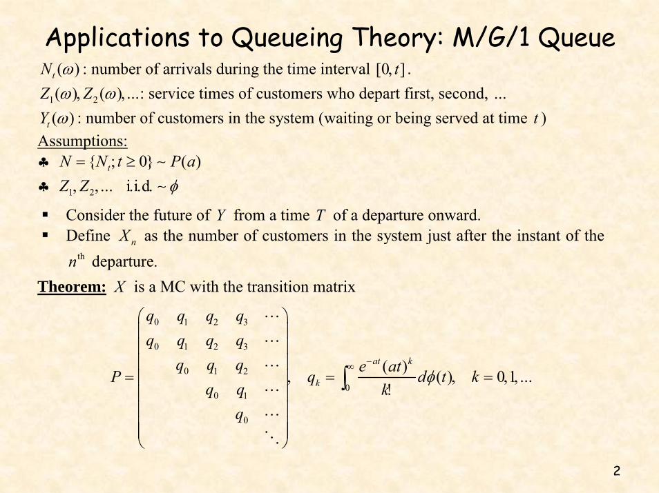
Applications to Queueing Theory: M/G/1 Queue( )tN ω : number of arrivals during the time interval [0 ]t, .

1 2( ) ( )Z Z …ω ω, , : service times of customers who depart first, second, … ( )tY ω : number of customers in the system (waiting or being served at time t )

Assumptions: ♣ { 0} ( )tN N t P a= ; ≥ ∼ ♣ 1 2 i i dZ Z … φ, , . . . ∼

Consider the future of Y from a time T of a departure onward. Define nX as the number of customers in the system just after the instant of the

thn departure.

Theorem: X is a MC with the transition matrix

0 1 2 3

0 1 2 3

0 1 2

00 1

0

( ) ( ) 0 1at k

k

q q q qq q q q

q q q e atP q d t k …q q k

q

φ−∞

⎛ ⎞⎜ ⎟⎜ ⎟⎜ ⎟

= , = , = , ,⎜ ⎟!⎜ ⎟

⎜ ⎟⎜ ⎟⎜ ⎟⎝ ⎠

∫

3

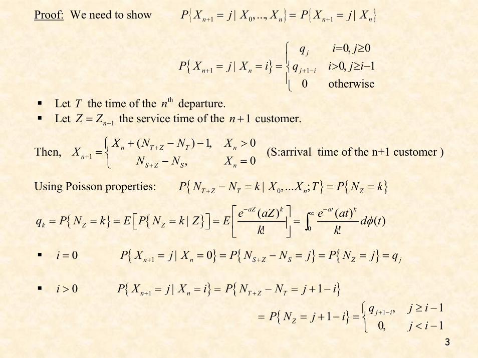
Proof: We need to show { }1 0n nP X j X … X+ = | , , = { }1n nP X j X+ = |

{ }1n nP X j X i+ = | = = 1

0 00 1

0 otherwise

j

j i

q i jq i j i+ −

= , ≥⎧⎪ > , ≥ −⎨⎪⎩

Let T the time of the thn departure. Let 1nZ Z += the service time of the 1n + customer.

Then, 1

( ) 1 00

n T Z T nn

S Z S n

X N N XX

N N X+

++

+ − − , >⎧= ⎨ − , =⎩

(S:arrival time of the n+1 customer )

Using Poisson properties: { } { }0T Z T n ZP N N k X …X T P N k+ − = | , ; = =

{ } { }0

( ) ( ) ( )aZ k at k

k Z Ze aZ e atq P N k E P N k Z E d t

k kφ

− −∞⎡ ⎤= = = = | = =⎡ ⎤ ⎢ ⎥⎣ ⎦ ! !⎣ ⎦

∫

0i = { } { } { }1 0n n S Z S Z jP X j X P N N j P N j q+ += | = = − = = = =

0i > { }1n nP X j X i+ = | = = { }1T Z TP N N j i+ − = + −

= { } 1 11

0 1j i

Z

q j iP N j i

j i+ − , ≥ −⎧

= + − = ⎨ , < −⎩

4

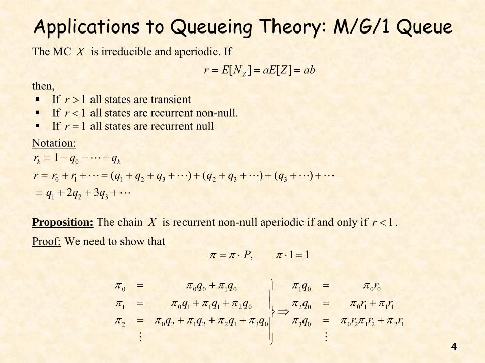
The MC X is irreducible and aperiodic. If

[ ] [ ]Zr E N aE Z ab= = =

then, If 1r > all states are transient If 1r < all states are recurrent non-null. If 1r = all states are recurrent null

Notation: kr = 01 kq q− − −

r = 0 1 1 2 3 2 3 3( ) ( ) ( )r r q q q q q q+ + = + + + + + + + + +

= 1 2 32 3q q q+ + +

Proposition: The chain X is recurrent non-null aperiodic if and only if 1r < .

Proof: We need to show that 1 1Pπ π π= ⋅ , ⋅ =

0 0 0 1 0 1 0 0 0

0 1 1 1 2 0 0 1 1 11 2 0

0 2 1 2 2 1 3 0 0 2 1 2 2 12 3 0

q q q rq q q q r r

q q q q q r r r

π π π π ππ π π π π π ππ π π π π π π π π

= + =⎫⎪= + + = +⎪⇒⎬= + + + = +⎪⎪⎭

Applications to Queueing Theory: M/G/1 Queue

5

Applications to Queueing Theory: M/G/1 Queue Summing all equations ( 0 01q r= − , 0 1 2r r r r= + + + )

0 0 01 1

(1 ) ( )j jj j

r r r rπ π π∞ ∞

= =

− ⋅ = + −∑ ∑

If 1r < , then we obtain 0 01 0

11 1j j

j j

rr r

π π π π∞ ∞

= =

= ⇒ =− −∑ ∑

The condition 1 1π ⋅ = is satisfied with 0 1 rπ = −

Theorem: The limits ( ) lim ( )nnj P i jπ →∞= , exist j E∀ ∈ and are independent of the

initial state i . • If 1r ≥ , then ( ) 0j jπ = , ∀ . • If 1r < , then

1 2

0

0

1

1 0

(0) 1

(1) (1 )

1( 1) (1 )k

jk

kj

a a ak S

rrrq

j r r r rq

π

π

π+

= ∈

= −

= −

⎛ ⎞+ = − ⎜ ⎟

⎝ ⎠∑ ∑

a

where jkS is the set of all k -tuples 1( )ka … a= , ,a of integers 1ia ≥ with 1 ka a j+ =

6

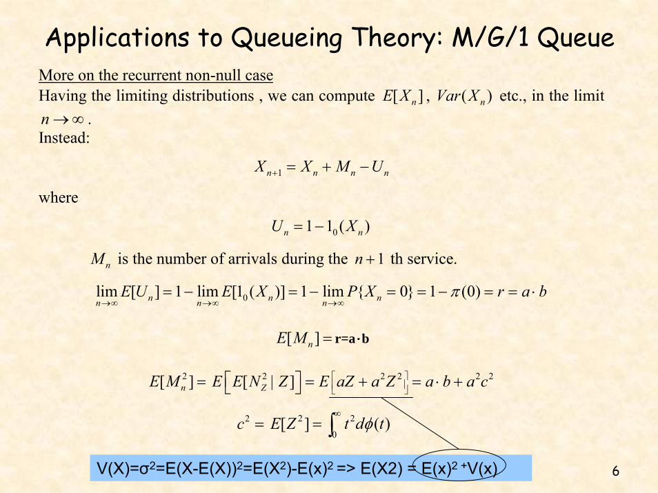
Applications to Queueing Theory: M/G/1 Queue More on the recurrent non-null case Having the limiting distributions , we can compute [ ]nE X , ( )nVar X etc., in the limitn→∞ . Instead:

1n n n nX X M U+ = + −

where

01 1 ( )n nU X= −

nM is the number of arrivals during the 1n + th service.

0lim [ ] 1 lim [1 ( )] 1 lim { 0} 1 (0)n n nn n nE U E X P X r a bπ

→∞ →∞ →∞= − = − = = − = = ⋅

[ ]nE M = r=a·b

2[ ]nE M = 2 2 2 2 2[ ]ZE E N Z E aZ a Z a b a c⎡ ⎤⎢ ⎥⎣ ⎦

⎡ ⎤| = + = ⋅ +⎣ ⎦

2c = 2 2

0[ ] ( )E Z t d tφ

∞= ∫

V(X)=σ2=E(X-E(X))2=E(X2)-E(x)2 => E(X2) = E(x)2 +V(x)

7

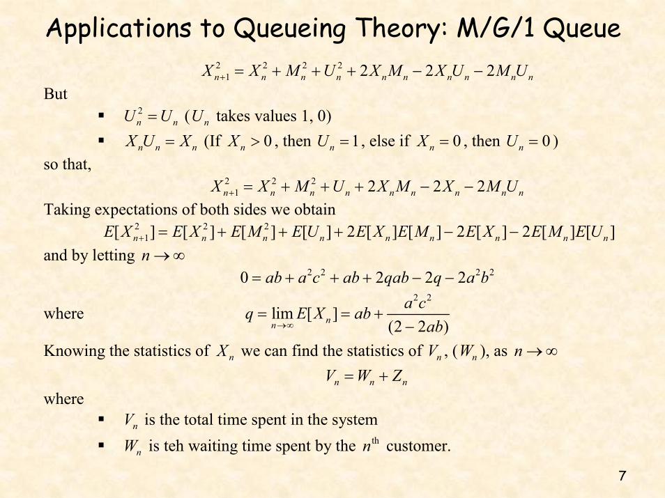
Applications to Queueing Theory: M/G/1 Queue 2 2 2 2

1 2 2 2n n n n n n n n n nX X M U X M X U M U+ = + + + − −

But 2

n nU U= ( nU takes values 1, 0) n n nX U X= (If 0nX > , then 1nU = , else if 0nX = , then 0nU = )

so that, 2 2 2

1 2 2 2n n n n n n n n nX X M U X M X M U+ = + + + − −

Taking expectations of both sides we obtain 2 2 2

1[ ] [ ] [ ] [ ] 2 [ ] [ ] 2 [ ] 2 [ ] [ ]n n n n n n n n nE X E X E M E U E X E M E X E M E U+ = + + + − −and by letting n→∞ 2 2 2 20 2 2 2ab a c ab qab q a b= + + + − −

where 2 2

lim [ ](2 2 )nn

a cq E X abab→∞

= = +−

Knowing the statistics of nX we can find the statistics of nV , ( nW ), as n→∞ n n nV W Z= +

where nV is the total time spent in the system nW is teh waiting time spent by the thn customer.

8

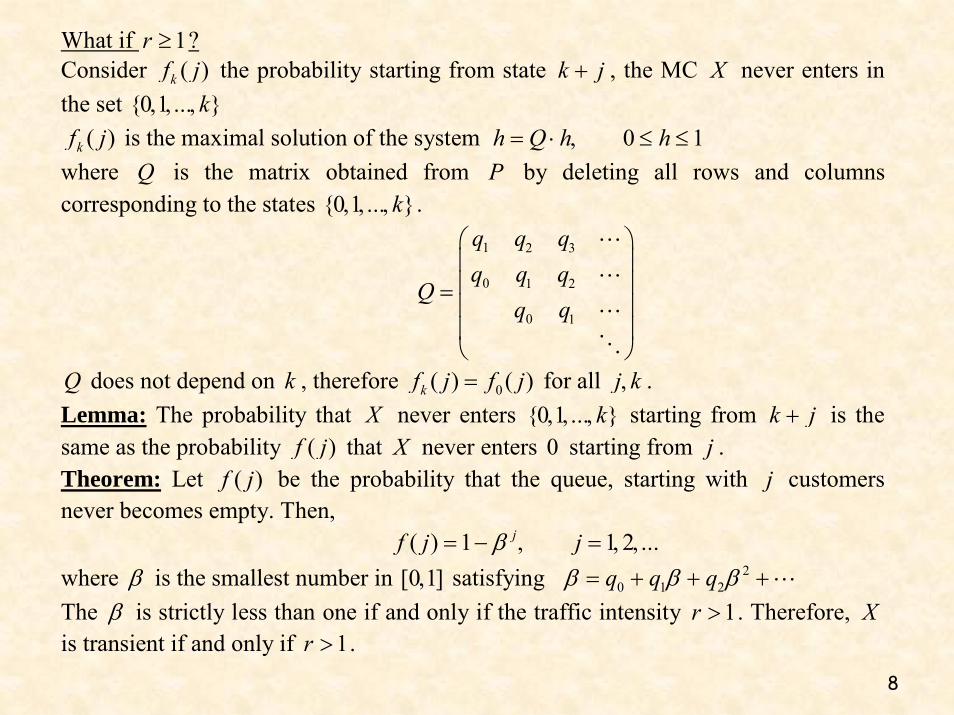
What if 1r ≥ ? Consider ( )kf j the probability starting from state k j+ , the MC X never enters inthe set {0 1 }… k, , ,

( )kf j is the maximal solution of the system 0 1h Q h h= ⋅ , ≤ ≤ where Q is the matrix obtained from P by deleting all rows and columnscorresponding to the states {0 1 }… k, , , .

1 2 3

0 1 2

0 1

q q qq q q

Qq q

⎛ ⎞⎜ ⎟⎜ ⎟=⎜ ⎟⎜ ⎟⎝ ⎠

Q does not depend on k , therefore 0( ) ( )kf j f j= for all j k, . Lemma: The probability that X never enters {0 1 }… k, , , starting from k j+ is thesame as the probability ( )f j that X never enters 0 starting from j . Theorem: Let ( )f j be the probability that the queue, starting with j customersnever becomes empty. Then, ( ) 1 1 2jf j j …β= − , = , ,

where β is the smallest number in [0 1], satisfying 20 1 2q q qβ β β= + + +

The β is strictly less than one if and only if the traffic intensity 1r > . Therefore, Xis transient if and only if 1r > .

9

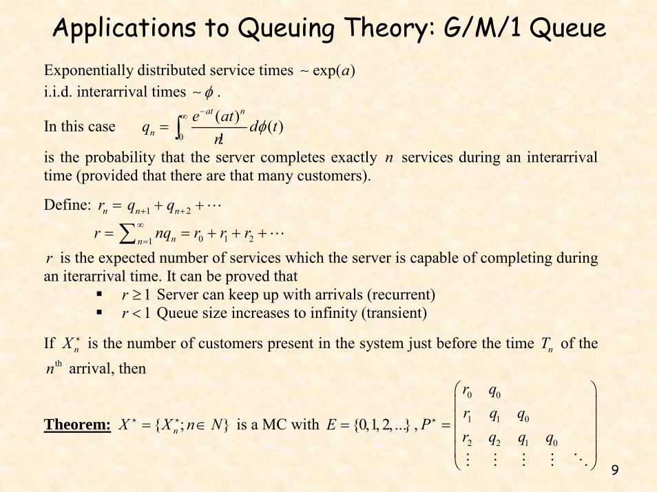
Applications to Queuing Theory: G/M/1 QueueExponentially distributed service times exp( )a∼ i.i.d. interarrival times φ∼ .

In this case 0

( ) ( )at n

ne atq d tn

φ−∞

=!∫

is the probability that the server completes exactly n services during an interarrivaltime (provided that there are that many customers).

Define: nr = 1 2n nq q+ ++ +

r = 0 1 21 nnnq r r r∞

== + + +∑

r is the expected number of services which the server is capable of completing duringan iterarrival time. It can be proved that

1r ≥ Server can keep up with arrivals (recurrent) 1r < Queue size increases to infinity (transient)

If nX is the number of customers present in the system just before the time nT of thethn arrival, then

Theorem: { }nX X n N= ; ∈ is a MC with {0 1 2 }E …= , , , ,

0 0

1 1 0

2 2 1 0

r qr q q

Pr q q q

⎛ ⎞⎜ ⎟⎜ ⎟=⎜ ⎟⎜ ⎟⎝ ⎠

10

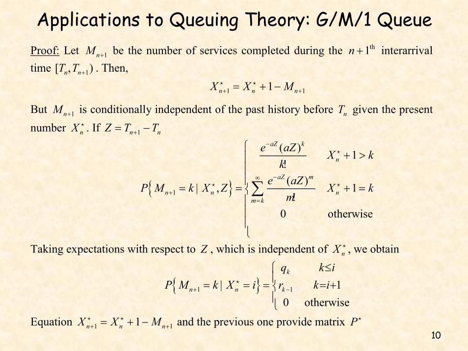
Applications to Queuing Theory: G/M/1 Queue Proof: Let 1nM + be the number of services completed during the th1n + interarrivaltime 1[ )n nT T +, . Then, 1 11n n nX X M+ += + −

But 1nM + is conditionally independent of the past history before nT given the presentnumber nX . If 1n nZ T T+= −

{ }1

( ) 1

( ), 1

0 otherwise

aZ k

n

aZ m

n n nm k

e aZ X kk

e aZP M k X Z X km

−

−∞

+=

⎧+ >⎪ !⎪

⎪= | = + =⎨

!⎪⎪⎪⎩

∑

Taking expectations with respect to Z , which is independent of nX , we obtain

{ }1 1 10 otherwise

k

n n k

q k iP M k X i r k i+ −

≤⎧⎪= | = = = +⎨⎪⎩

Equation 1 11n n nX X M+ += + − and the previous one provide matrix P

11

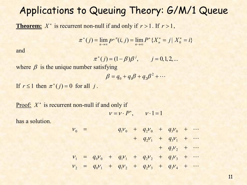
Applications to Queuing Theory: G/M/1 Queue Theorem: X is recurrent non-null if and only if 1r > . If 1r > , 0( ) lim ( ) lim { }n

nn nj i j P X j X iPπ

→∞ →∞= , = = | =

and ( ) (1 ) 0 1 2jj j …π β β= − , = , , , where β is the unique number satisfying 2

0 1 2q q qβ β β= + + +

If 1r ≤ then ( ) 0jπ = for all j .

Proof: X is recurrent non-null if and only if 1 1Pν ν ν= ⋅ , ⋅ = has a solution.

0 1 0 2 0 3 0

2 1 3 1

3 2

1 0 0 1 1 2 2 3 3

2 0 1 1 2 2 3 3 4

q q qq q

qq q q qq q q q

ν ν ν νν ν

νν ν ν ν νν ν ν ν ν

= + + ++ + +

+ += + + + += + + + +

12

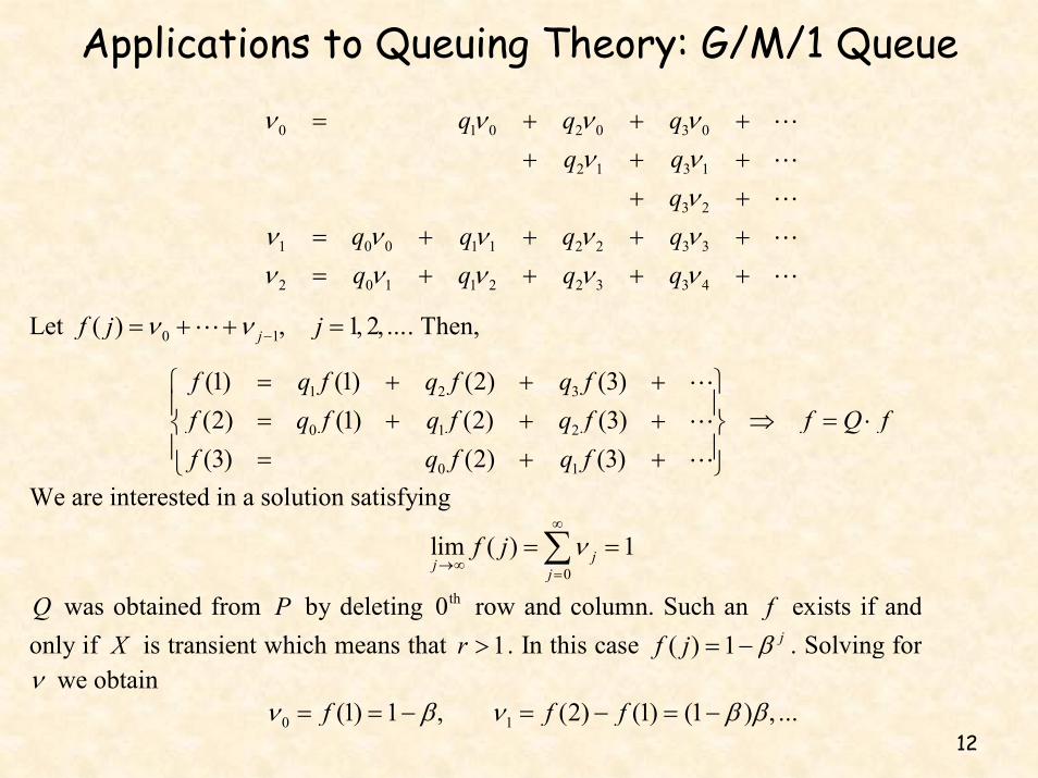
Applications to Queuing Theory: G/M/1 Queue

0 1 0 2 0 3 0

2 1 3 1

3 2

1 0 0 1 1 2 2 3 3

2 0 1 1 2 2 3 3 4

q q qq q

qq q q qq q q q

ν ν ν νν ν

νν ν ν ν νν ν ν ν ν

= + + ++ + +

+ += + + + += + + + +

Let 0 1( ) 1 2jf j j …ν ν −= + + , = , , . Then,

1 2 3

0 1 2

0 1

(1) (1) (2) (3)(2) (1) (2) (3)(3) (2) (3)

f q f q f q ff q f q f q f f Q ff q f q f

= + + +⎧ ⎫⎪ ⎪= + + + ⇒ = ⋅⎨ ⎬⎪ ⎪= + +⎩ ⎭

We are interested in a solution satisfying

0

lim ( ) 1jj jf j ν

∞

→∞=

= =∑

Q was obtained from P by deleting th0 row and column. Such an f exists if andonly if X is transient which means that 1r > . In this case ( ) 1 jf j β= − . Solving forν we obtain 0 1(1) 1 (2) (1) (1 )f f f …ν β ν β β= = − , = − = − ,

13

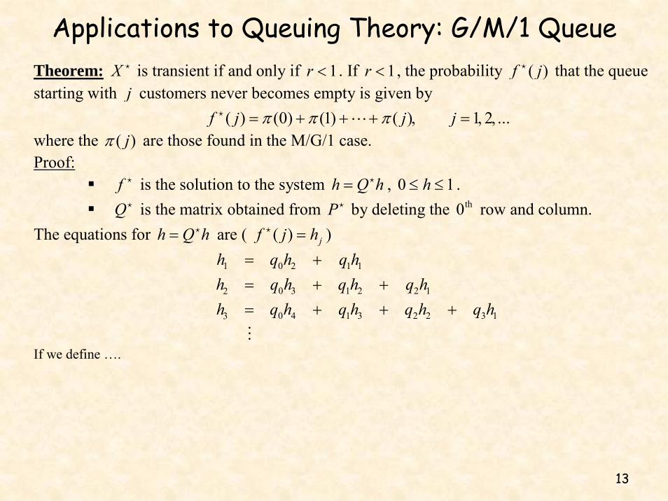
Applications to Queuing Theory: G/M/1 Queue Theorem: X is transient if and only if 1r < . If 1r < , the probability ( )f j that the queue

starting with j customers never becomes empty is given by ( ) (0) (1) ( ) 1 2f j j j …π π π= + + + , = , , where the ( )jπ are those found in the M/G/1 case. Proof:

f is the solution to the system h Q h= , 0 1h≤ ≤ . Q is the matrix obtained from P by deleting the th0 row and column.

The equations for h Q h= are ( ( ) jf j h= )

1 0 2 1 1

0 3 1 2 2 12

0 4 1 3 2 2 3 13

h q h q hh q h q h q hh q h q h q h q h

= += + += + + +

If we define ….

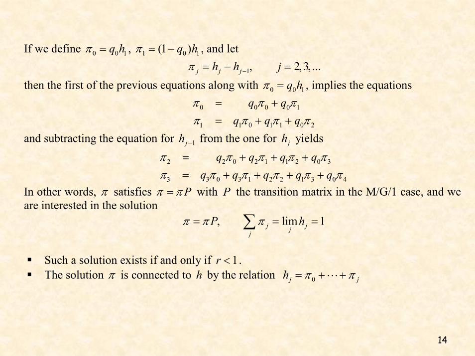
14

If we define 0 0 1q hπ = , 1 0 1(1 )q hπ = − , and let 1 2 3j j jh h j …π −= − , = , ,

then the first of the previous equations along with 0 0 1q hπ = , implies the equations

0 0 0 0 1

1 0 1 1 0 21

q qq q q

π π ππ π π π

= += + +

and subtracting the equation for 1jh − from the one for jh yields

2 2 0 2 1 1 2 0 3

3 0 3 1 2 2 1 3 0 43

q q q qq q q q q

π π π π ππ π π π π π

= + + += + + + +

In other words, π satisfies Pπ π= with P the transition matrix in the M/G/1 case, and weare interested in the solution lim 1j jjj

P hπ π π= , = =∑

Such a solution exists if and only if 1r < . The solution π is connected to h by the relation 0j jh π π= + +

15

Special case M/M/1 We can consider this queue as a special case of M/G/1 or G/M/1. In the sequel we useG/M/1. Now the interarrival distribution is given by:

( ) 1 0tt e tλφ −= − , ≥

To compute the limiting distribution of X (queue size just before the thn arrival, we findfirst β , where

0

kk

kqβ β

∞

=

= =∑ ( )0 0

at ke atk tkk

e dtλβ λ−∞∞ −

!=∑ ∫ = (1 )

0

at ta ae e dtβ λ λ

λ βλ∞ − − −

+ −=∫

The previous equation becomes or (1 )( ) 0aba aλβ β λ

λ β= − − =

+ −

with solutions 1β = and aλβ = . When 1ar λ= > , the smallest solution is

aλβ =

So we have { }lim 1 0 1j

nnP X j j …

a aλ λ

→∞

⎛ ⎞⎛ ⎞= = − , = , ,⎜ ⎟⎜ ⎟⎝ ⎠⎝ ⎠

It turns out that { }lim 1 0 1j

ttP Y j j …

a aλ λ

→∞

⎛ ⎞⎛ ⎞= = − , = , ,⎜ ⎟⎜ ⎟⎝ ⎠⎝ ⎠

for the queue size tY at time t .

and { }lim 1 0 1j

nnP X j j …

a aλ λ

→∞

⎛ ⎞⎛ ⎞= = − , = , ,⎜ ⎟⎜ ⎟⎝ ⎠⎝ ⎠

for the queue size nX just after the thn departure.

16

Birth and Death Processes

Introduction to Stochastic Processes (Erhan Cinlar)Ch. 8.6

17

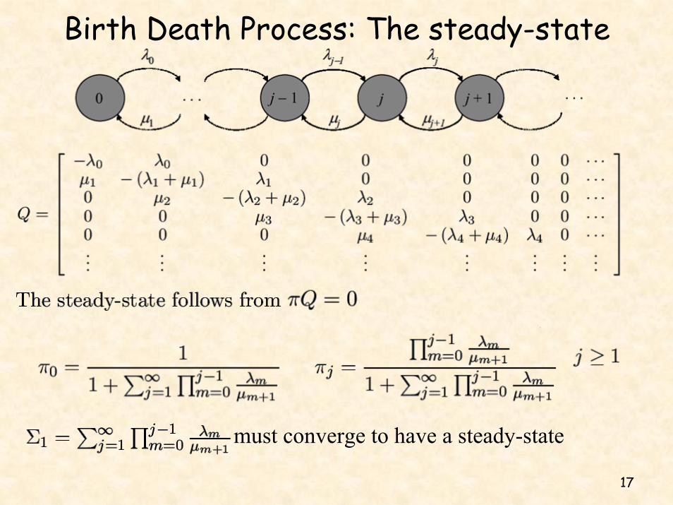
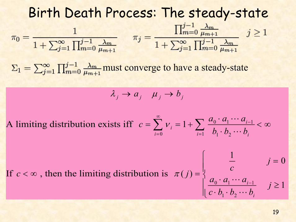
Birth Death Process: The steady-state

must converge to have a steady-state

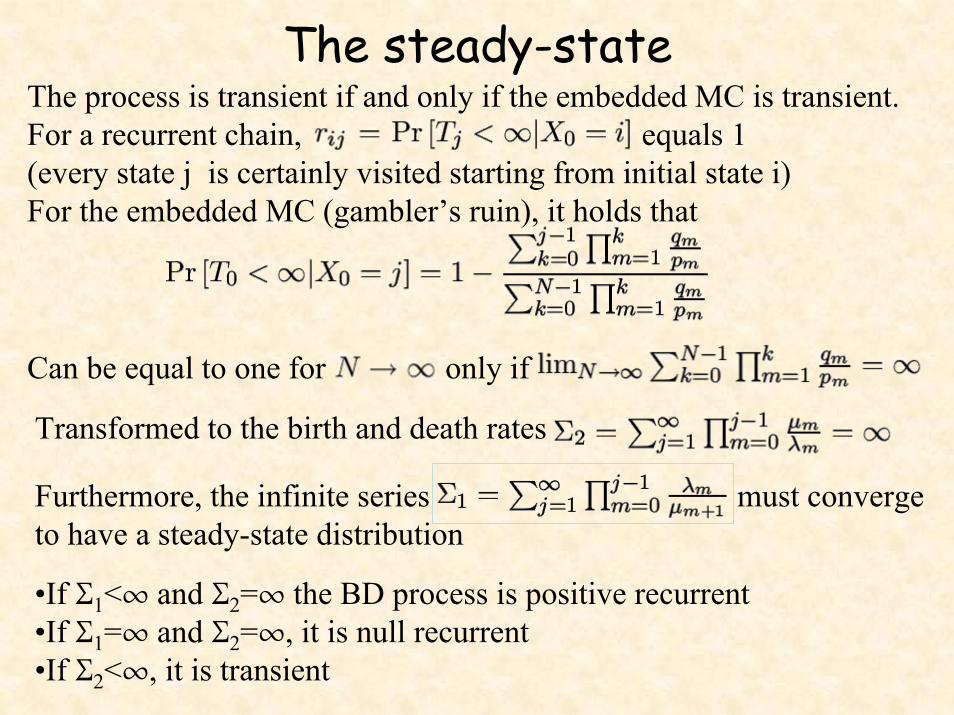
The steady-stateThe process is transient if and only if the embedded MC is transient.For a recurrent chain, equals 1(every state j is certainly visited starting from initial state i)For the embedded MC (gambler’s ruin), it holds that

Can be equal to one for only if

Transformed to the birth and death rates

Furthermore, the infinite series must converge to have a steady-state distribution

•If S1<¶ and S2=¶ the BD process is positive recurrent •If S1=¶ and S2=¶, it is null recurrent•If S2<¶, it is transient

19

Birth Death Process: The steady-state

must converge to have a steady-state

j j j ja bλ μ→ →

A limiting distribution exists iff 0 1 1

0 1 1 2

1 ii

i i i

a a acb b b

ν∞

−

= =

⋅= = + < ∞

⋅∑ ∑

If c < ∞ , then the limiting distribution is 0 1 1

1 2

1 0( )

1i

i

jcj a a a j

c b b b

π−

⎧ =⎪⎪= ⎨ ⋅⎪ ≥⋅ ⋅⎪⎩

20

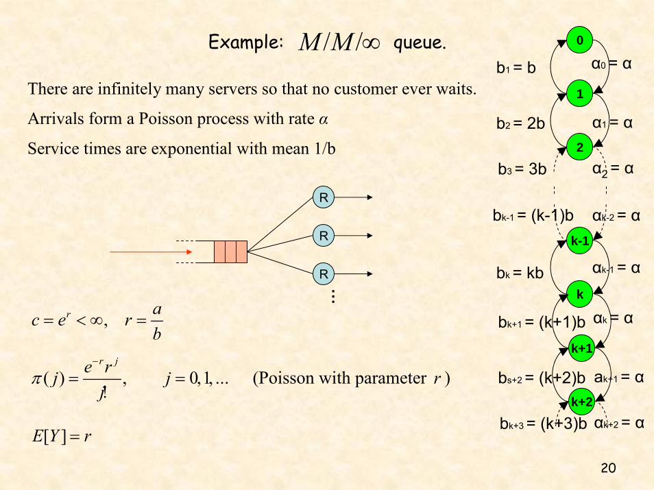
Example: queue.M M/ /∞

There are infinitely many servers so that no customer ever waits.

Arrivals form a Poisson process with rate α

Service times are exponential with mean 1/b

,r ac e rb

= < ∞ =

( ) 0 1r je rj j …j

π−

= , = , ,!

(Poisson with parameter r )

[ ]E Y r=

R

R

R...

0

1

2

k-1

k

α0 = α

α1 = α

α2 = α

αk-1 = α

b2 = 2b

b1 = b

b3 = 3b

bk = kb

bk-1 = (k-1)b αk-2 = α

k+1

k+2

αk = α

ak+1 = α

αk+2 = α

bs+2 = (k+2)b

bk+1 = (k+1)b

bk+3 = (k+3)b

21

Example: queue.

0 0

1 1 1 1

2 2 2 2 2 2

a ab a b a

Qb a b a

a ab a b a

b a b a

−⎛ ⎞⎜ ⎟− −⎜ ⎟⎜ ⎟− −⎜ ⎟⎝ ⎠

−⎛ ⎞⎜ ⎟− −⎜ ⎟= =⎜ ⎟− −⎜ ⎟⎝ ⎠

0

*0 1 1

1 01 2 1

1! !

1

nx

n

i

i i

x enari ib

ri

i i

a rc ei b

a a ab b ib

∞

=

=!

= ∞

== =

−

∑⋅

+= = =⋅

+ =∑ ∑∑

0 1 1

1 2

1 0( ) , or ( )

1 !1! !

1r j

j j r

r j rj

i

je rj ja r e jj

e j

ca a ac b b b b e j

π π−

⎧ = =⎪⎪= =⎨⎪ = = ≥⎩

⋅⎪ ⋅ ⋅

M M/ /∞

0

*1

0 1 1 0

[ ]! ( 1) ! !

nx

n

x en

j j kr r r r

j rj j j k

r r rE Y j j e r e r e re re j j k

π

∞

=

=!

−∞ ∞ ∞ ∞− − −

= = = =

∑

= = = = = =−∑ ∑ ∑ ∑

22

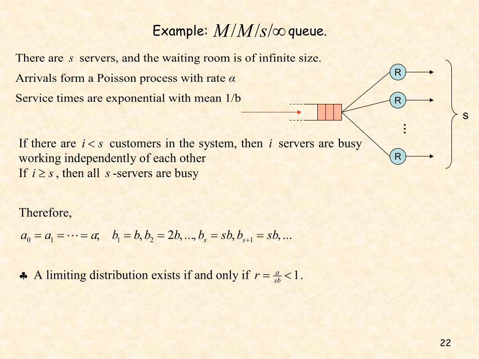
Example: queue.M M s/ / /∞There are s servers, and the waiting room is of infinite size.

Arrivals form a Poisson process with rate α

Service times are exponential with mean 1/b

If there are i s< customers in the system, then i servers are busyworking independently of each other If i s≥ , then all s -servers are busy

Therefore,

0 1 1 2 12 s sa a a b b b b … b sb b sb …+= = = ; = , = , , = , = ,

♣ A limiting distribution exists if and only if 1a

sbr = < .

R

R

R

...s

23

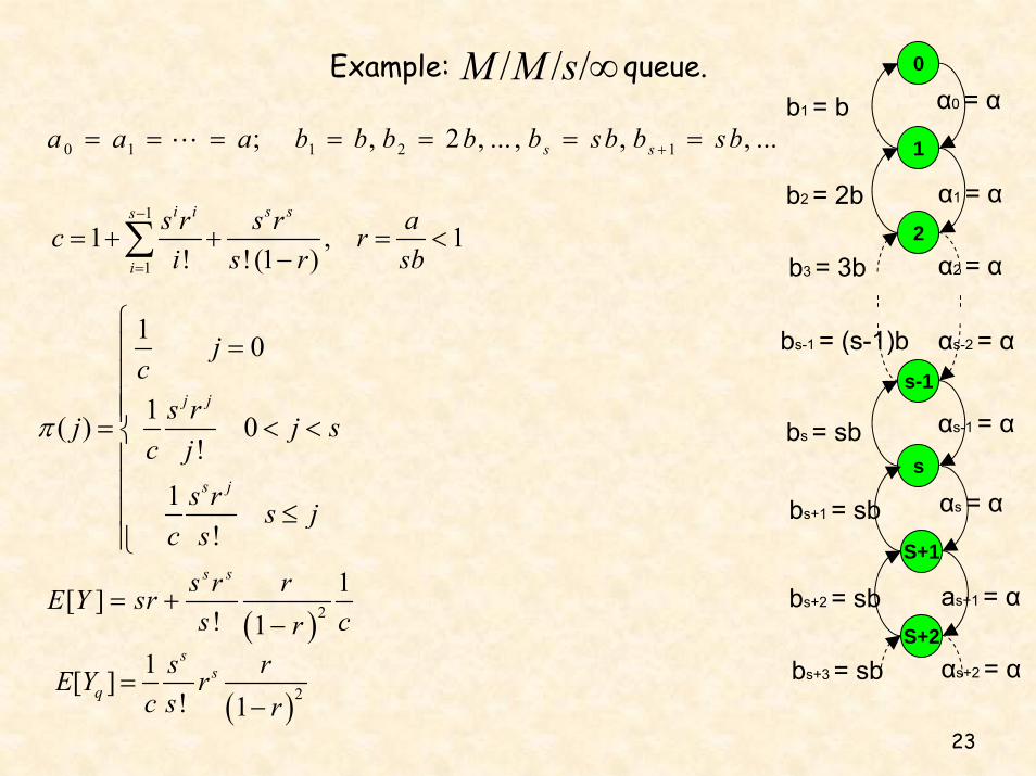
Example: queue.M M s/ / /∞

0 1 1 2 12 s sa a a b b b b … b sb b sb …+= = = ; = , = , , = , = ,

0

1

2

s-1

s

α0 = α

α1 = α

α2 = α

αs-1 = α

b2 = 2b

b1 = b

b3 = 3b

bs = sb

bs-1 = (s-1)b αs-2 = α

S+1

S+2

αs = α

as+1 = α

αs+2 = α

bs+2 = sb

bs+1 = sb

bs+3 = sb

1

1

1 , 1! !(1 )

i i s ss

i

s r s r ac ri s r sb

−

=

= + + = <−∑

1 0

1( ) 0!

1!

j j

s j

jcs rj j sc js r s jc s

π

⎧=⎪

⎪⎪⎪= < <⎨⎪⎪

≤⎪⎪⎩

( )21[ ]

! 1

s ss r rE Y srs cr

= +−

( )21[ ]

! 1

ss

qs rE Y r

c s r=

−

24

Example: queue.M M s/ / /∞An arriving customer is permitted to balk: if he finds the systemtoo crowded, he may leave, but once he joins the system hecannot change his mind later. Suppose the probability of joining the queue is ip if there are i -customers in the system at the time of arrival.

s

R

R

R

...pi

1-pi

i

Ιf the queue size at time t is tY i= , and if there were no service completions during [ ]t t u, + , then the probability that there are no additions to the queue during [ ]t t u, + is

0

* (1 )

0 0

( (1 ))( ) (1 )

nx

n

i i

x en

nau nau p ap un au aui

in n

au pe au p e e e en n

∞

=

=!

−∞ ∞− −− −

= =

∑−

− = = =! !∑ ∑

0

1

2

s-1

s

α0 = αp0

α1 = α p1

α3 = α p2

αs-1 = α ps-1

b2 = 2b

b1 = b

b3 = 3b

bs = sb

bs-1 = (s-1)b αs-2 = α ps-2

S+1

S+2

αs = α ps

as+1 = α ps+1

αs+2 = α ps+2

bs+2 = sb

bs+1 = sb

bs+3 = sb

Hence, 0 0 1 1

1 2 1 22i i

s s s

a ap a ap …a apb b b b … b sb b b sb+ +

= , = , =

= , = , , = , = = =

25

tY is a special birth-death process, where

0 1 2 1 2a a a a b b b= = = = ; = = =

The parameter abr = is called traffic intensity.

If 1abr = < , then there is a limiting distribution, which is

1 01( )

11

j

j

jcj c

ra jcb

π

⎧ =⎪⎪= , =⎨ −⎪ ≥⎪⎩

Thus, ( ) (1 ) jj r rπ = − , j=0, 1, …

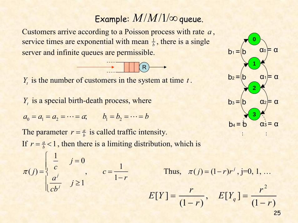
Example: queue.Customers arrive according to a Poisson process with rate a , service times are exponential with mean 1

b , there is a single server and infinite queues are permissible. tY is the number of customers in the system at time t .

1M M/ / /∞

0

1

2

3

α0 = α

α1 = α

α2 = α

α3 = α

b2 = b

b1 = b

b4 = b

b3 = b

R

2

[ ] , [ ](1 ) (1 )qr rE Y E Yr r

= =− −

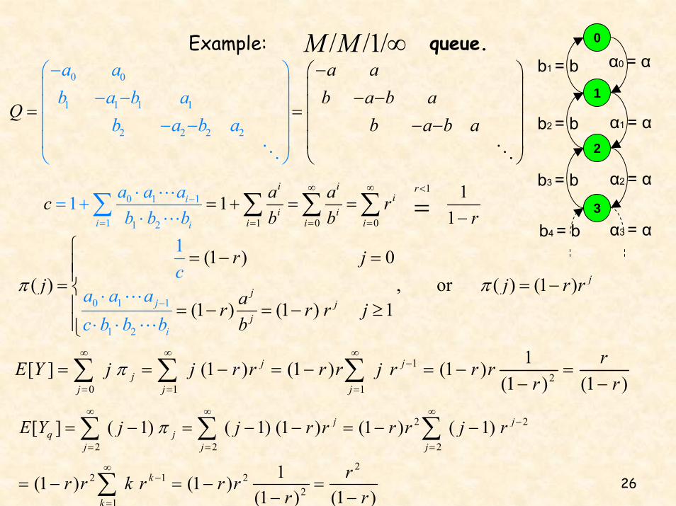
26

Example: queue.0 0

1 1 1 1

2 2 2 2

a ab a b a

Qb

a ab a b a

b a b a a b a

−⎛ ⎞ −⎛ ⎞⎜ ⎟− −⎜ ⎟= =⎜ ⎟− −⎜ ⎟⎝

⎜ ⎟− −⎜ ⎟⎜

⎠

⎟− −⎜ ⎟⎝ ⎠

1

1 0

0 1 1

1 1 2 0

1 111

i i ri

i ii i

i

i ii

a ac rb b r

a a ab b b

∞ ∞ <

= =

−

= =

= +−

⋅==

⋅=+ ∑ ∑ ∑ =∑

0 1 1

1 2

(1 ) 0( ) , or

1

( ) (1 )(1 ) (1 ) 1

jj

jjj

i

r jj j r r

ac

a a ac b b

r r jbb

rπ π

−

⎧ = − =⎪⎪= = −⎨⎪ = − =

⋅−

⋅ ⋅≥

⎪⎩

0

1

2

3

α0 = α

α1 = α

α2 = α

α3 = α

b2 = b

b1 = b

b4 = b

b3 = b

1M M/ / /∞

2 2

2 2 2

22 1 2

21

[ ] ( 1) ( 1) (1 ) (1 ) ( 1)

1(1 ) (1 )(1 ) (1 )

j jq j

j j j

k

k

E Y j j r r r r j r

rr r k r r rr r

π∞ ∞ ∞

−

= = =

∞−

=

= − = − − = − −

= − = − =− −

∑ ∑ ∑

∑

12

0 1 1

1[ ] (1 ) (1 ) (1 )(1 ) (1 )

j jj

j j j

rE Y j j r r r r j r r rr r

π∞ ∞ ∞

−

= = =

= = − = − = − =− −∑ ∑ ∑

27

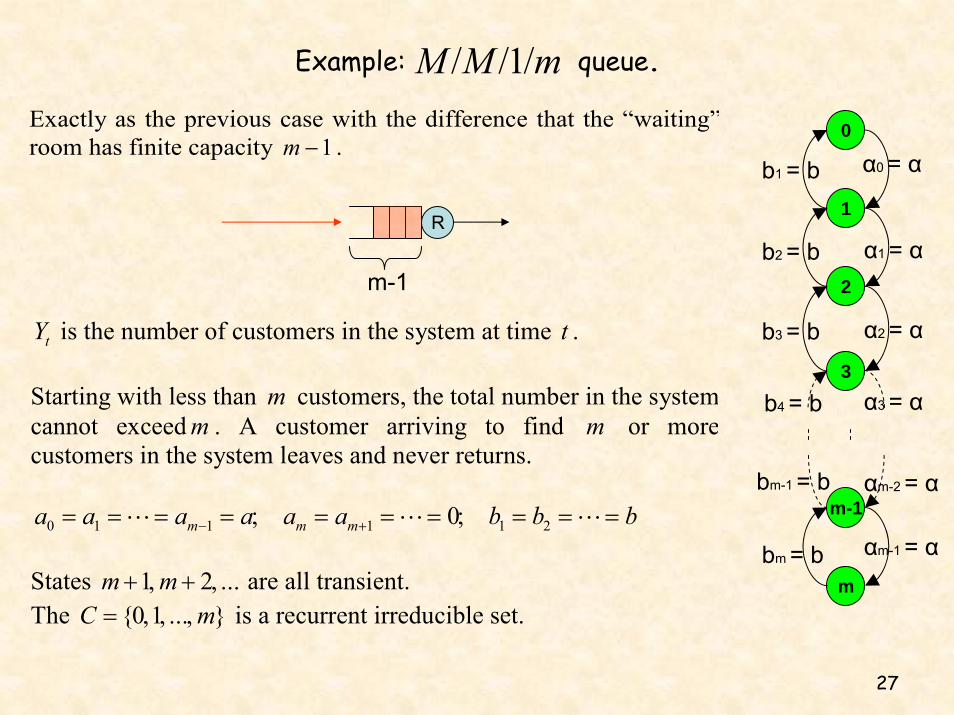
Example: queue. 1M M m/ / /Exactly as the previous case with the difference that the “waiting”room has finite capacity 1m − .

0

1

2

3

m-1

m

α0 = α

α1 = α

α2 = α

α3 = α

αm-1 = α

b2 = b

b1 = b

b4 = b

b3 = b

bm = b

bm-1 = b αm-2 = α

tY is the number of customers in the system at time t . Starting with less than m customers, the total number in the systemcannot exceedm . A customer arriving to find m or morecustomers in the system leaves and never returns.

0 1 1 1 1 20m m ma a a a a a b b b− += = = = ; = = = ; = = =

States 1 2m m …+ , + , are all transient. The {0 1 }C … m= , , , is a recurrent irreducible set.

R

m-1

28

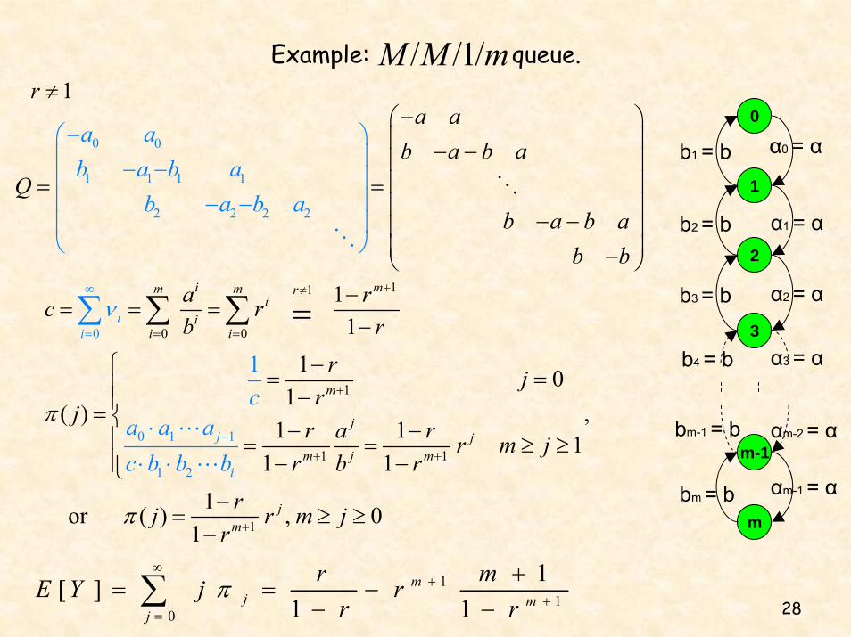
Example: queue.1M M m/ / /

0

1

2

3

m-1

m

α0 = α

α1 = α

α2 = α

α3 = α

αm-1 = α

b2 = b

b1 = b

b4 = b

b3 = b

bm = b

bm-1 = b αm-2 = α

0 0

1 1 1 1

2 2 2 2

a ab a b a

b a b a

a ab a b a

Qb a b a

b b

−⎛ ⎞⎜ ⎟− −⎜ ⎟⎜ ⎟

−⎛ ⎞⎜ ⎟− −⎜ ⎟⎜ ⎟= =⎜ ⎟

− −⎜ ⎟⎜ ⎟−⎝

− −⎜ ⎟⎝ ⎠

⎠11

0 00

11

i mm m ri

ii i

ii

a rc rb r

ν+≠

=

∞

= =

−= = =

−∑ ∑ =∑

1

1 1

1

0 1 1

1 2

1 01

( ) ,1 1 1

1 11or (

1

1

) , 0

j

m

jj

m j m

jm

i

r jr

jr a r r m jr

ca a ac b r

rj r

b b b

m jr

π

π

+

+

+

−+

−⎧ = =⎪ −⎪= ⎨ − −⎪ = = ≥ ≥⎪ −

⋅

⋅ ⋅ −⎩−

= ≥ ≥−

1r ≠

11

0

1[ ]1 1

mj m

j

r mE Y j rr r

π∞

++

=

+= = −

− −∑

29

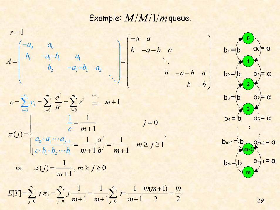
Example: queue. 1M M m/ / /

0

1

2

3

m-1

m

α0 = α

α1 = α

α2 = α

α3 = α

αm-1 = α

b2 = b

b1 = b

b4 = b

b3 = b

bm = b

bm-1 = b αm-2 = α

0 0

1 1 1 1

2 2 2 2

a ab a b a

b a b a

a ab a b a

Ab a b a

b b

−⎛ ⎞⎜ ⎟− −⎜ ⎟⎜ ⎟

−⎛ ⎞⎜ ⎟− −⎜ ⎟⎜ ⎟= =⎜ ⎟

− −⎜ ⎟⎜ ⎟−⎝

− −⎜ ⎟⎝ ⎠

⎠1

0 0 0

1i

im m ri

ii ii

ac r mb

ν=

= =

∞

=

= = = +∑ ∑ ∑ =

0 1 1

1 2

1 01

( ) ,1 1 1

1 11or ( ) , 0

1

1

jj

j

i

jm

ja m j

m b

ca a ac m

j m

b

m

b b

j

π

π

−

⎧ = =⎪ +⎪= ⎨⎪ = = ≥ ≥⎪ + +

⋅

⋅ ⋅⎩

= ≥ ≥+

1r =

0 0 0

1 1 1 ( 1)[ ]1 1 1 2 2

m m

jj j j

m m mE Y j j jm m m

π∞

= = =

+= = = = =

+ + +∑ ∑ ∑

30

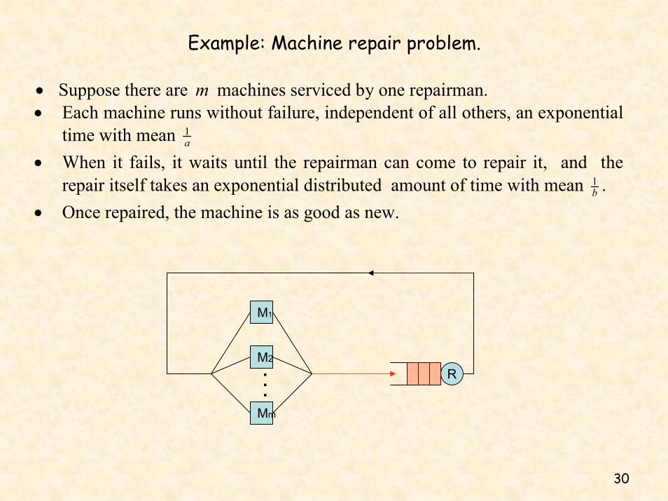
• Suppose there are m machines serviced by one repairman. • Each machine runs without failure, independent of all others, an exponential

time with mean 1a

• When it fails, it waits until the repairman can come to repair it, and the repair itself takes an exponential distributed amount of time with mean 1

b . • Once repaired, the machine is as good as new.

Example: Machine repair problem.

M1

M2...

R

Mm

31

• Let tY be the number of failed machines at time t • If tY i= , then there are m i

Example: Machine repair problem.

− machines working, and the time until the next failure is exponential withparameter ( )m i a− (if no machines are repaired in themeantime).

Hence, 0 1 1 1

1 2

( 1) ; ( 0)m m ma ma a m a … a a a ab b b

− +• = , = − , , = = = =

• = = =

Limiting distribution:

( ) ( 1) ( ) 0 1jaj pm m m j j … m

bπ ⎛ ⎞= − − , = , , ,⎜ ⎟

⎝ ⎠

where 0

1 ( 1) ( )im

i

am m m ip b=

⎛ ⎞= − − ⎜ ⎟⎝ ⎠

∑

0

1

2

3

m-1

m

α0 = m α

α1 = (m-1) α

α2 = (m-2) α

α3 = (m-3) α

αm-1 = α

b2 = b

b1 = b

b4 = b

b3 = b

bm = b

bm-1 = b αm-2 = 2 α