Introduction to Series-Parallel Duality

David Ellerman University of California at Riverside

www.ellerman.org May 2004 Abstract

The parallel sum of two positive real numbers x:y = [(1/x) + (1/y)]-1 arises in electrical circuit theory as the resistance resulting from hooking two resistances x and y in parallel. There is a duality between the usual (series) sum and the parallel sum. The reciprocity map ρ taking x to 1/x is an "anti-isomorphism" of the positive reals onto itself in the sense that the map swaps the sums: ρ(x:y) = [x:y]-1 = (1/x) + (1/y) = ρ(x)+ρ(y), while it preserves multiplication: ρ(xy) = ρ(x)ρ(y). This duality allows one to dualize any statement involving the two sums and multiplication. For example, this yields a duality theory for financial arithmetic (where the pairing of basic functions and their reciprocals has been previously noticed without the explanation of the underlying series-parallel duality). Geometrically, positive scalars can be represented as positively sloped straight lines through the origin which can be generalized to increasing functions. The multiplication of scalars becomes the composition of functions and the reciprocal of a scalar becomes the inverse of a function. The series and parallel sum then become the vertical and horizontal sums of increasing functions. The duality transformation (the reciprocity map on scalars) is carried out by rotating the graph around the 450 line. Since the derivative of a convex function is an increasing function, we then show how an convex function and its convex conjugate have derivatives that are series-parallel duals. Table of Contents Introduction to Parallel Addition

Series Chauvinism Parallel Sums in High School Math The Harmonic Mean

Series-Parallel Duality The Reciprocity Map Dual Equations on the Positive Reals

Series and Parallel Geometric Series Geometric Interpretation of Parallel Sum Solutions of Linear Equations: Geometric Interpretation Duality in Financial Arithmetic

Parallel Sums in Financial Arithmetic Future Values and Sinking Fund Deposits Infinite Streams of Payments Application: The Faustmann-Ohlin-Gaffney Steady-state Forest Problem

Economic Duality and Convex Conjugate Functions References

Introduction to Parallel Addition In economic theory, "duality" means "convex duality," which includes duality in linear and non-linear programming as special cases. Series-parallel duality has been studied largely in electrical circuit theory and, to some extent, in combinatorial theory. Series-parallel duality also occurs in economics and finance, and it is related to convex duality as the derivative of a function is related to the function (anti-derivative). When resistors with resistances a and b are placed in series, their compound resistance is the usual sum (hereafter the series sum) of the resistances a+b. If the resistances are placed in parallel, their compound resistance is the parallel sum of the resistances, which is denoted by the full colon:

( ) .

b1

a1

1bab:a111

+=+=

−−−

����������������a

b ����������������������������������������������������������������������������������������������������������������a:b = (1/a + 1/b)

-1

����������������a b

����������������������������������������a + b

��������������������������������������������������������������������������

����������������������������������������������������������������������������������

Series and Parallel Sums

The parallel sum is associative x:(y:z)) = (x:y):z, commutative x:y = y:x, and distributive x(y:z) = xy:xz. On the positive reals, there is no identity element for either sum but the "closed circuit" 0 and the "open circuit" ∞ can be added to form the extended positive reals. Those elements are the identity elements for the two sums, x+0 = x = x:∞. For fractions, the series sum is the usual addition expressed by the annoyingly asymmetrical rule: "Find the common denominator and then add the numerators." The parallel sum of fractions restores symmetry since it is defined in the dual fashion: "Find the common numerator and then (series) add the denominators."

ab

ad

ab d

: =+

The parallel sum of fractions can also be obtained by finding the common denominator and taking the parallel sum of numerators.

ab

cb

a cb

: :=

The usual series sum of fractions can be obtained by finding the common numerator and then taking the parallel sum of the denominators.

ab

ad

ab d

+ =:

2

The rules for series and parallel sums of fractions can be summarized in the following four equations which restore full symmetry.

a b a b a b a b

a b a b a b a b

1 1 1 1 1 1

1 1 1 1 1 1

+ =+

=

=+

+ =

: :

::

Series Chauvinism

From the viewpoint of pure mathematics, the parallel sum is "just as good" as the series sum. It is only for empirical and perhaps even some accidental reasons that so much mathematics is developed using the series sum instead of the equally good parallel sum. There is a whole "parallel mathematics" which can be developed with the parallel sum replacing the series sum. Since the parallel sum can be defined in terms of the series sum (or vice-versa), "parallel mathematics" is essentially a new way of looking at certain known parts of mathematics. Exclusive promotion of the series sum is "series chauvinism" or "serialism." Before venturing further into the parallel universe, we might suggest some exercises to help the reader combat the heritage of series chauvinism. Anytime the series sum seems to occur naturally in mathematics with the parallel sum nowhere in sight, it is an illusion. The parallel sum lurks in a "parallel" role that has been unfairly neglected. For instance, a series chauvinist might point out that the series sum appears naturally in the rule for working with exponents xaxb = xa+b while the parallel sum does not. But this is only an illusion due to our mathematically arbitrary symmetry-breaking choice to take exponents to represent powers rather than roots. Let a pre-superscript stand for a root (just as a post-superscript stands for a power) so 2x would be the square root of x. Then the rule for working with these exponents is axbx = a:bx so the parallel sum does have a role symmetrical to the series sum in the rules for working with exponents.

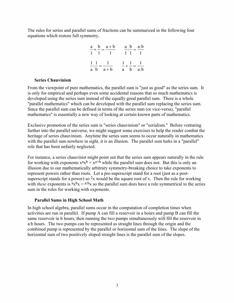
Parallel Sums in High School Math

In high school algebra, parallel sums occur in the computation of completion times when activities are run in parallel. If pump A can fill a reservoir in a hours and pump B can fill the same reservoir in b hours, then running the two pumps simultaneously will fill the reservoir in a:b hours. The two pumps can be represented as straight lines through the origin and the combined pump is represented by the parallel or horizontal sum of the lines. The slope of the horizontal sum of two positively sloped straight lines is the parallel sum of the slopes.

3

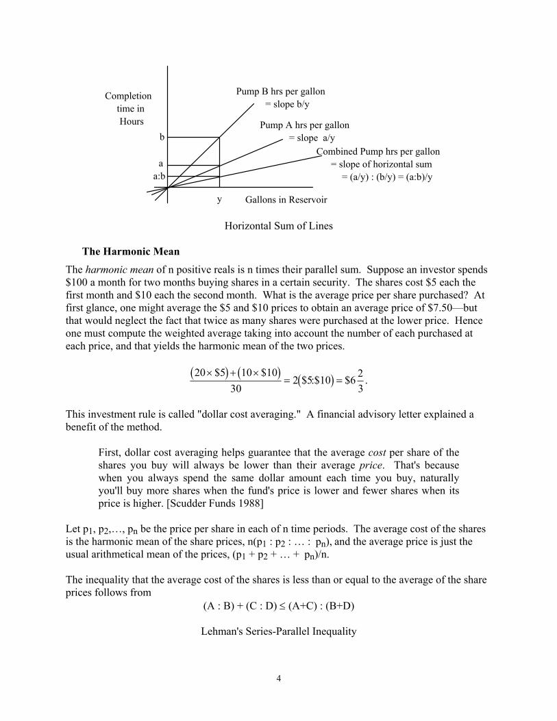
b

a a:b

Gallons in Reservoir

Completion time in Hours Pump A hrs per gallon

= slope a/y

Pump B hrs per gallon = slope b/y

Combined Pump hrs per gallon = slope of horizontal sum

= (a/y) : (b/y) = (a:b)/y

y

Horizontal Sum of Lines

The Harmonic Mean

The harmonic mean of n positive reals is n times their parallel sum. Suppose an investor spends $100 a month for two months buying shares in a certain security. The shares cost $5 each the first month and $10 each the second month. What is the average price per share purchased? At first glance, one might average the $5 and $10 prices to obtain an average price of $7.50—but that would neglect the fact that twice as many shares were purchased at the lower price. Hence one must compute the weighted average taking into account the number of each purchased at each price, and that yields the harmonic mean of the two prices.

( ) ( ) ( )20 1030

2 23

× + ×= =

$5 $10$5:$10 $6 .

This investment rule is called "dollar cost averaging." A financial advisory letter explained a benefit of the method.

First, dollar cost averaging helps guarantee that the average cost per share of the shares you buy will always be lower than their average price. That's because when you always spend the same dollar amount each time you buy, naturally you'll buy more shares when the fund's price is lower and fewer shares when its price is higher. [Scudder Funds 1988]

Let p1, p2,…, pn be the price per share in each of n time periods. The average cost of the shares is the harmonic mean of the share prices, n(p1 : p2 : … : pn), and the average price is just the usual arithmetical mean of the prices, (p1 + p2 + … + pn)/n. The inequality that the average cost of the shares is less than or equal to the average of the share prices follows from

(A : B) + (C : D) ≤ (A+C) : (B+D)

Lehman's Series-Parallel Inequality

4

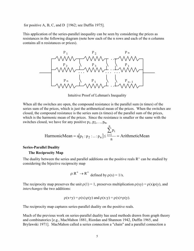
for positive A, B, C, and D [1962; see Duffin 1975]. This application of the series-parallel inequality can be seen by considering the prices as resistances in the following diagram (note how each of the n rows and each of the n columns contains all n resistances or prices).

p 1

p 2

p n

p 3

p 1

p 2

p n p 1

p n − 1

... ... ...

...

...

...

Intuitive Proof of Lehman's Inequality

When all the switches are open, the compound resistance is the parallel sum (n times) of the series sum of the prices, which is just the arithmetical mean of the prices. When the switches are closed, the compound resistance is the series sum (n times) of the parallel sum of the prices, which is the harmonic mean of the prices. Since the resistance is smaller or the same with the switches closed, we have for any positive p1, p2,…, pn,

[ ] MeanArithmeticMeanHarmonicn

pp:...:p:pn

n

1ii

n21 ==∑=≤

Series-Parallel Duality The Reciprocity Map

The duality between the series and parallel additions on the positive reals R+ can be studied by considering the bijective reciprocity map

ρ:R R+ +→ defined by ρ(x) = 1/x.

The reciprocity map preserves the unit ρ(1) = 1, preserves multiplication ρ(xy) = ρ(x)ρ(y), and interchanges the two additions:

ρ(x+y) = ρ(x):ρ(y) and ρ(x:y) = ρ(x)+ρ(y).

The reciprocity map captures series-parallel duality on the positive reals. Much of the previous work on series-parallel duality has used methods drawn from graph theory and combinatorics [e.g., MacMahon 1881, Riordan and Shannon 1942, Duffin 1965, and Brylawski 1971]. MacMahon called a series connection a "chain" and a parallel connection a

5

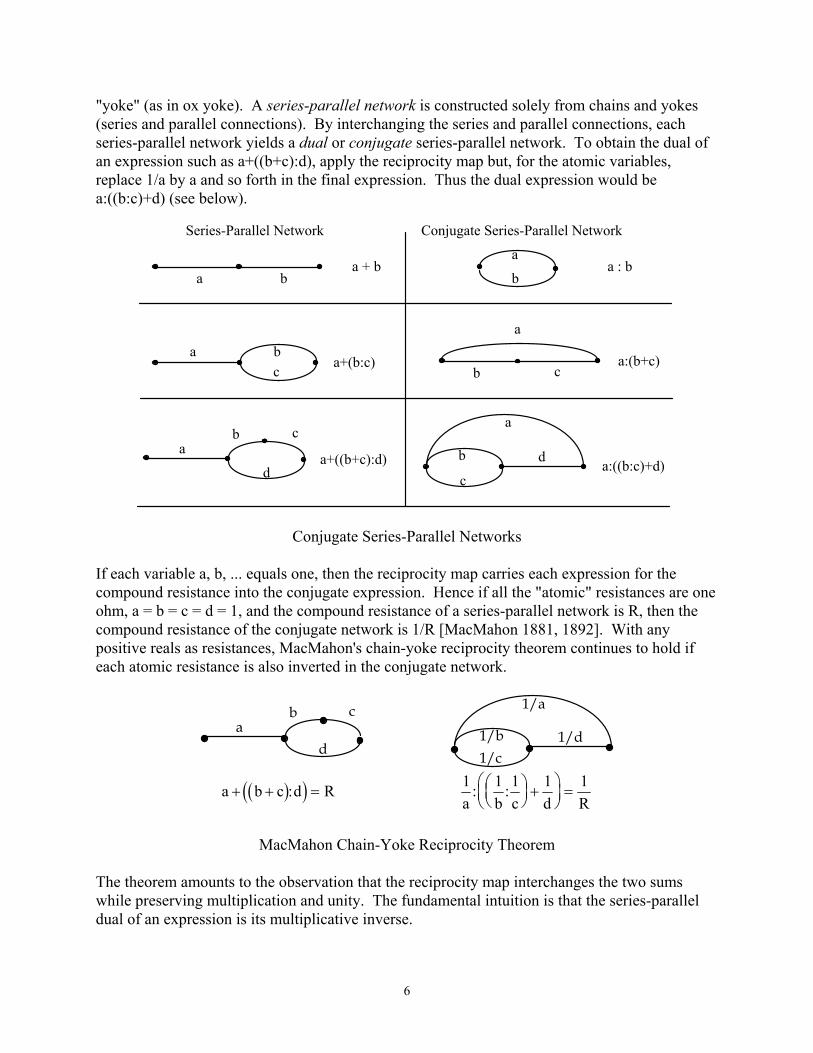
"yoke" (as in ox yoke). A series-parallel network is constructed solely from chains and yokes (series and parallel connections). By interchanging the series and parallel connections, each series-parallel network yields a dual or conjugate series-parallel network. To obtain the dual of an expression such as a+((b+c):d), apply the reciprocity map but, for the atomic variables, replace 1/a by a and so forth in the final expression. Thus the dual expression would be a:((b:c)+d) (see below).

Series-Parallel Network Conjugate Series-Parallel Network

a b

a

b a : b a + b

a b c a+(b:c)

a

b c a:(b+c)

· a b c

d a+((b+c):d) a:((b:c)+d)

a

b

c

d

Conjugate Series-Parallel Networks

If each variable a, b, ... equals one, then the reciprocity map carries each expression for the compound resistance into the conjugate expression. Hence if all the "atomic" resistances are one ohm, a = b = c = d = 1, and the compound resistance of a series-parallel network is R, then the compound resistance of the conjugate network is 1/R [MacMahon 1881, 1892]. With any positive reals as resistances, MacMahon's chain-yoke reciprocity theorem continues to hold if each atomic resistance is also inverted in the conjugate network.

a b c

d

1/a

1/b 1/c

1/d

( )( )a b c d+ + =: R 1 1 1 1 1a b c d R

: :

+

=

MacMahon Chain-Yoke Reciprocity Theorem

The theorem amounts to the observation that the reciprocity map interchanges the two sums while preserving multiplication and unity. The fundamental intuition is that the series-parallel dual of an expression is its multiplicative inverse.

6

Dual Equations on the Positive Reals

Any equation on the positive reals concerning the two sums and multiplication can be dualized by applying the reciprocity map to obtain another equation. The series sum and parallel sum are interchanged. For example, the equation

13

5 25

35

2+ +

=

dualizes to the equation

3 15

52

53

12

: :

= .

The following equation

( )1 1 1 1= + +

xx

:

holds for any positive real x. Add any x to one and add its reciprocal to one. The results are two numbers larger than one and their parallel sum is exactly one. Dualizing yields the equation

( )1 1 1 1=

+: :x

x

for all positive reals x. Taking the parallel sum of any x and its reciprocal with one yields two numbers smaller than one which sum to one. For any set of positive reals x1,...,xn, the parallel summation can be expressed using the capital P:

i

ni i

i

n

P x x=

−

=

−

=

∑

1

1

1

1

.

Parallel Summation The binomial theorem

( )a bnk

a bn

k

nk n k+ =

=

−∑0

dualizes to the parallel sum binomial theorem (where "1/a" is replaced by "a" and similarly for "b"):

( )a bnk

a bn

k

nk n kP: .=

=

−−

0

1

Parallel Sum Binomial Theorem

7

Taking a = 1+x and b = 1 + 1/x (and using a previous equation on the left-hand side), we have a nonobvious identity

( ) ( )1 1 1 10

1=

+ +

=

− −

k

n k n kP

nk

x x

for any x > 0.

Series and Parallel Geometric Series The following formula (and its dual) for partial sums of geometric series (starting at i = 1) are useful in financial mathematics (where x is any positive real).

( ) ( )( ) ( )( )nn1n

0i

in

1i

i x:11x)x:1(1

x:11)x:1()x:1()x:1(x:1 −=−

−== ∑∑

−

==

Partial Sums of Geometric Series

Dualizing yields a formula for partial sums of parallel-sum geometric series. The dual of the series subtraction a–b where a > b is the parallel subtraction x\y = [1/x – 1/y]-1 where x < y.

( ) ( ) ( )( ) .

)x1(1x

x1\1x1(\1)x1(x1)x1(x1 n

ni

1n

0i

in

1iPP −

−

== +−=

++

+=++=+

Partial Sums of Dual Geometric Series

Dualization can also be applied to infinite series. Taking the limit as n→∞ in the above partial sum formulas yields for any positive reals x the dual summation formulas for series and parallel sum geometric series that begin at the index i = 1.

( ) ( )1 11 1

:x x xi

i i

iP=

∞

=

∞∑ = = +

The parallel sum series in the above equation can be used to represent a repeating decimal as a fraction. An example will illustrate the procedure so let z = .367367367… where the "367" repeats. Then since 1/a + 1/b = 1/(a:b), we have:

( ) ( )z i

i

i

iP= = =

=

∞

=

∞∑. .367367 367

1000

367

10001

1

K

Taking y = x+1 for x > 0 in the previous geometric series equation yields

8

i

iP y y=

∞= −

11

for y > 1 which is applied to yield

( ).

999367

11000367

1000

367367367.zi

1iP

=−

===∞

=

K

For any positive real x, the beautiful dual formulas for the geometric series with indices beginning at i = 0 can be obtained by serial or parallel adding 1= (1:x)0 = (1+x)0 to each side.

( ) (1 10

:x xi

i=

∞

∑ = + )

): .

Geometric Series for any Positive Real x

( ) (i

iP x x=

∞+ =

01 1

Dual Geometric Series for any Positive Real x

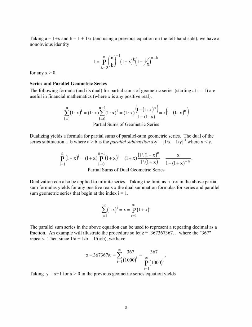
Geometric Interpretation of Parallel Sum The harmonic mean of two numbers is twice their parallel sum, just as the usual series or arithmetical mean is half their series sum. The geometric interpretation of the harmonic mean will lead us into geometric applications of the parallel sum. Draw a line FG through the point E where the diagonals cross in the trapezoid ABDC.

A B

C D

E F G

Geometry of Parallel Sum

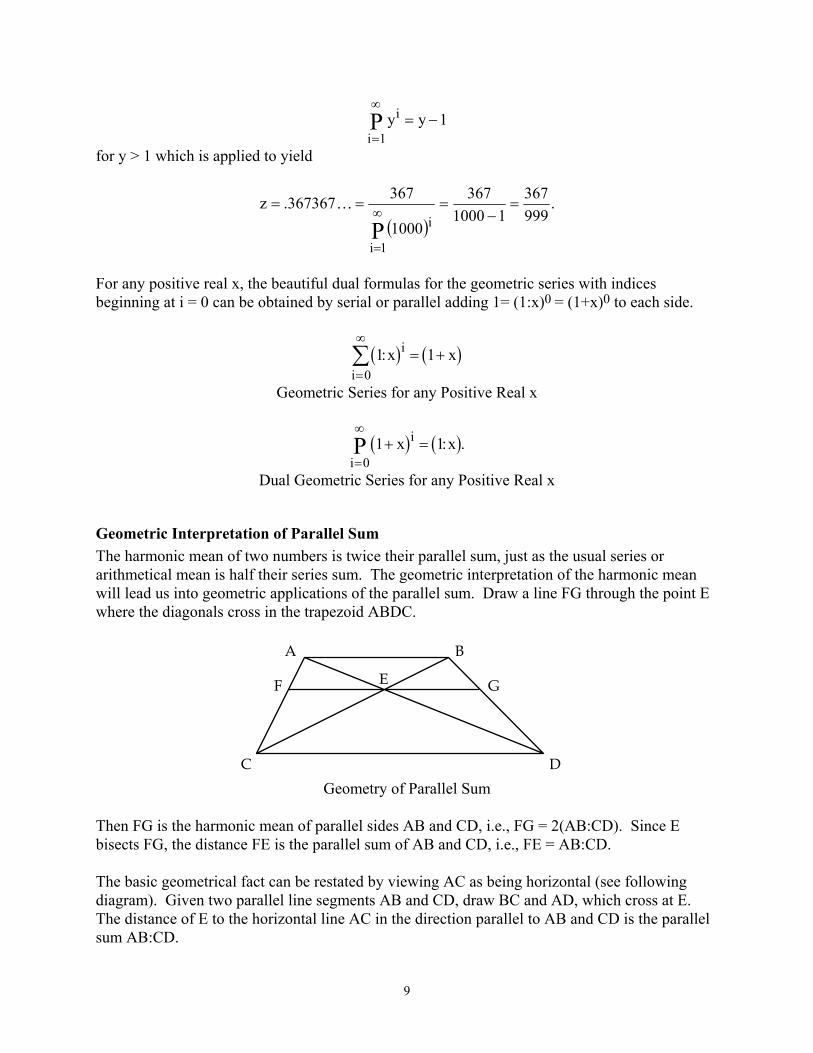
Then FG is the harmonic mean of parallel sides AB and CD, i.e., FG = 2(AB:CD). Since E bisects FG, the distance FE is the parallel sum of AB and CD, i.e., FE = AB:CD. The basic geometrical fact can be restated by viewing AC as being horizontal (see following diagram). Given two parallel line segments AB and CD, draw BC and AD, which cross at E. The distance of E to the horizontal line AC in the direction parallel to AB and CD is the parallel sum AB:CD.

9

A

B

C

D

E

F

EF = AB:CD

It is particularly interesting to note that the distance AC is arbitrary. If CD is shifted out parallel to C'D' and the new diagonals AD' and BC' are drawn (as if rubber bands connected B with C and A with D), then the distance E'F' is again the parallel sum of AB and CD (= C'D').

A

B

C

D

E

F C'

D'

E'

F' EF = E'F' = AB:CD where CD = C'D'

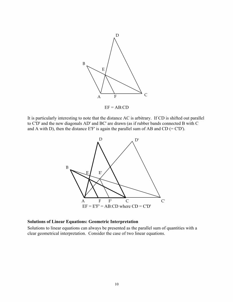
Solutions of Linear Equations: Geometric Interpretation Solutions to linear equations can always be presented as the parallel sum of quantities with a clear geometrical interpretation. Consider the case of two linear equations.

10

A

B

C

D

E

F

x 2

x 1

Linear Equations and Parallel Sum EF = AB:CD

For instance, the x2 solution EF is the parallel sum of AB and CD, which are the "pillars" that rise up to each line from where the other line hits the x1 floor. This procedure generalizes to any nonsingular system of n linear equations. Suppose we wish to find the solution value of xj. Each of the linear equations defines a hyperplane in n-space. For each i = 1,…,n, the n-1 hyperplanes taken by excluding the ith hyperplane intersect to form a line which, in turn, intersects the xj = 0 floor at some point called the "base of the ith pillar." The perpendicular distance from that base point on the xj = 0 floor up to the ith hyperplane is the height cj(i) of the "ith pillar" (on the xj = 0 floor). If the perpendicular line through the base point does not intersect the ith hyperplane, then the height cj(i) of the ith pillar can be taken as ∞ ("∞" is "open circuit" element that is the identity for the parallel sum, ∞ : x = x, and absorbs under the series sum, ∞ + x = ∞). The parallel sum of the pillars is the solution value of xj:

cj(1) : cj(2) : … : cj(n) = xj solution.

For i = 1,…,n, the base of the ith pillar is the solution of the system of equations if the ith equation is replaced by xj = 0. Now solve the ith equation for xj when the other variables are set at their "base of the ith pillar" values. That value is the ith pillar cj(i). Thus the ith pillar measures the effect of the ith equation on determining xj if the role of xj if the other variables are fixed at their "base of the ith pillar" values. The parallel sum of these isolated effects is the xj solution. The proof of this result uses Cramer’s Rule. Consider each column of a square matrix A = [aij ] as a (reversible) linear activity that uses n inputs supplied in given amounts (the bi constants). The jth activity is given by a column vector (a1j,…,anj)T (where the "T" superscript indicates transpose). Each unit of the jth activity uses up aij units of the ith input. With given input supplies b = (b1,…,bn)T, the levels of the n activities x = (x1,…,xn)T are determined by the matrix equation Ax = b. To isolate the effect of the jth activity on using the ith input, replace the jth activity by the column (0,…,0,aij,0,…,0)T so we only consider the effect of the jth activity on using the ith input (where

11

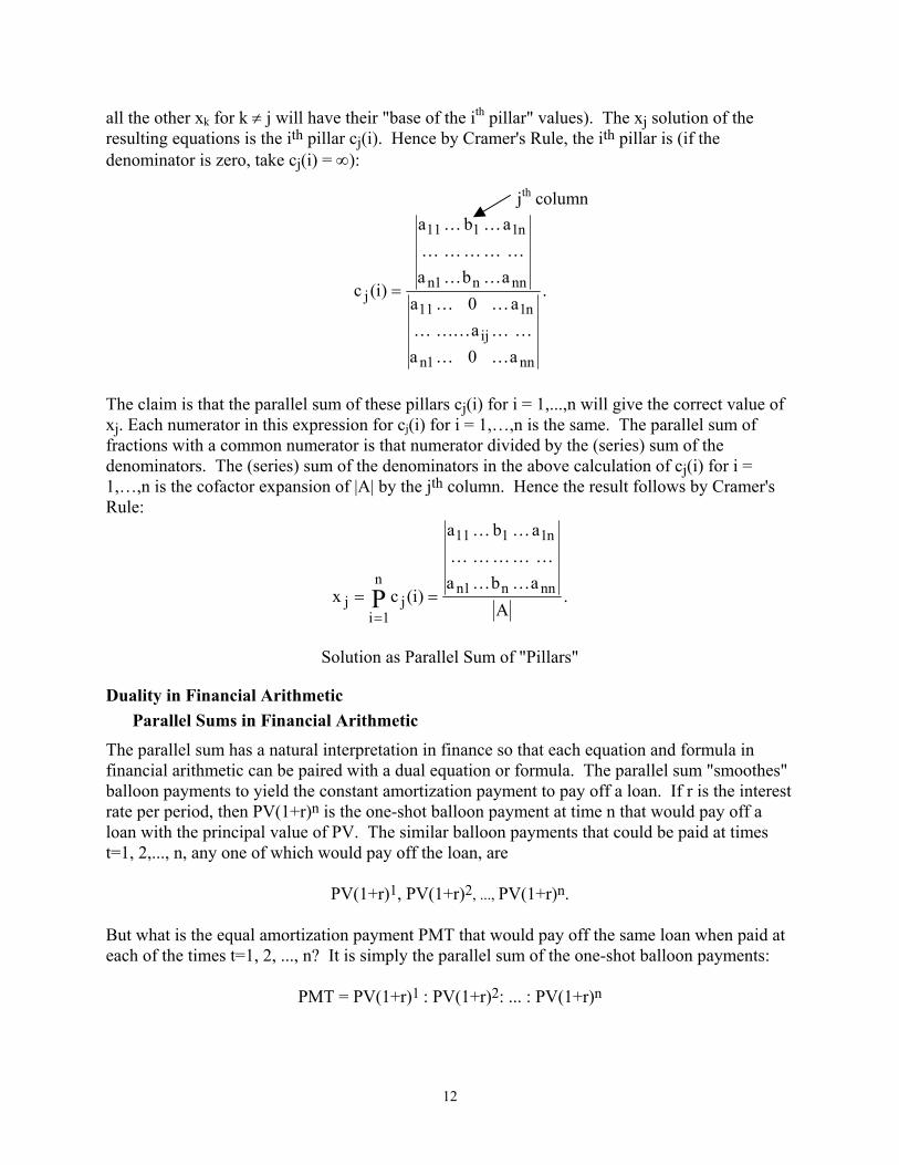
all the other xk for k ≠ j will have their "base of the ith pillar" values). The xj solution of the resulting equations is the ith pillar cj(i). Hence by Cramer's Rule, the ith pillar is (if the denominator is zero, take cj(i) = ∞):

n

0a0

a

aa

a

b

b

a

a

)i(c

ij

1n

11

n

1

1n

11

j

K

K

K

K

K

K

K

K

K

K

K

K

K

K

K

K

K

=

The claim is that the parallel sum of these pillars cj(i) forxj. Each numerator in this expression for cj(i) for i = 1,…fractions with a common numerator is that numerator divdenominators. The (series) sum of the denominators in th1,…,n is the cofactor expansion of |A| by the jth column. Rule:

Ab

b

a

a

)i(cx n

1

1n

11

jn

1ij P

K

K

K

K

K

===

Solution as Parallel Sum o

Duality in Financial Arithmetic Parallel Sums in Financial Arithmetic

The parallel sum has a natural interpretation in finance sofinancial arithmetic can be paired with a dual equation orballoon payments to yield the constant amortization paymrate per period, then PV(1+r)n is the one-shot balloon payloan with the principal value of PV. The similar balloon t=1, 2,..., n, any one of which would pay off the loan, are

PV(1+r)1, PV(1+r)2, ..., P

But what is the equal amortization payment PMT that woeach of the times t=1, 2, ..., n? It is simply the parallel su

PMT = PV(1+r)1 : PV(1+r)2:

12

jth colum

.

a

a

nn

n1

nn

n1

K

i = 1,...,n will give the correct value of ,n is the same. The parallel sum of ided by the (series) sum of the e above calculation of cj(i) for i =

Hence the result follows by Cramer's

.a

a

nn

n1K

K

K

K

f "Pillars"

that each equation and formula in formula. The parallel sum "smoothes" ent to pay off a loan. If r is the interest ment at time n that would pay off a payments that could be paid at times

V(1+r)n.

uld pay off the same loan when paid at m of the one-shot balloon payments:

... : PV(1+r)n

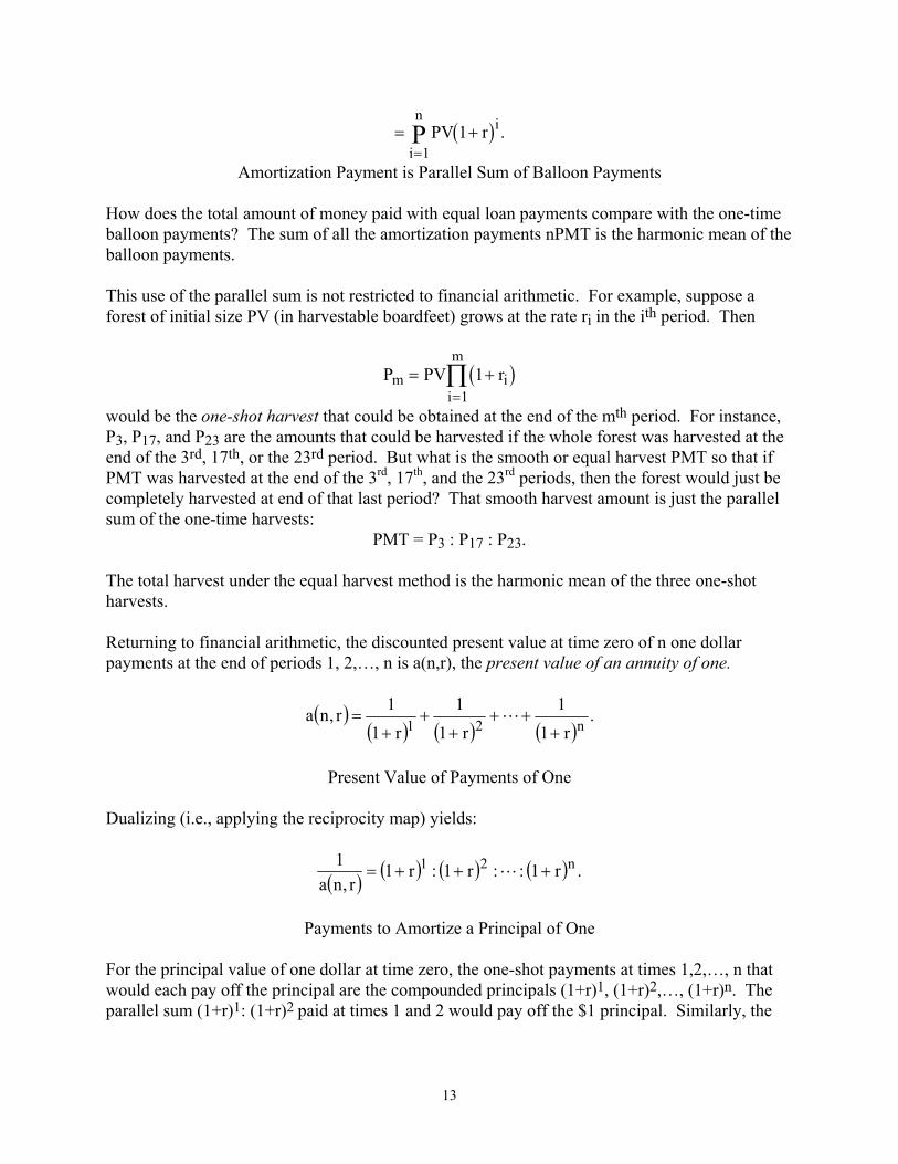
( )= +=i

n iP PV r1

1 .

Amortization Payment is Parallel Sum of Balloon Payments

How does the total amount of money paid with equal loan payments compare with the one-time balloon payments? The sum of all the amortization payments nPMT is the harmonic mean of the balloon payments. This use of the parallel sum is not restricted to financial arithmetic. For example, suppose a forest of initial size PV (in harvestable boardfeet) grows at the rate ri in the ith period. Then

( )P PV rm ii

m= +

=∏ 1

1 would be the one-shot harvest that could be obtained at the end of the mth period. For instance, P3, P17, and P23 are the amounts that could be harvested if the whole forest was harvested at the end of the 3rd, 17th, or the 23rd period. But what is the smooth or equal harvest PMT so that if PMT was harvested at the end of the 3rd, 17th, and the 23rd periods, then the forest would just be completely harvested at end of that last period? That smooth harvest amount is just the parallel sum of the one-time harvests:

PMT = P3 : P17 : P23.

The total harvest under the equal harvest method is the harmonic mean of the three one-shot harvests. Returning to financial arithmetic, the discounted present value at time zero of n one dollar payments at the end of periods 1, 2,…, n is a(n,r), the present value of an annuity of one.

( )( ) ( ) ( )

.r1

1r1

1r1

1r,na n21 +++

++

+= L

Present Value of Payments of One

Dualizing (i.e., applying the reciprocity map) yields:

( ) ( ) ( ) ( ) .r1::r1:r1r,na

1 n21 +++= L

Payments to Amortize a Principal of One

For the principal value of one dollar at time zero, the one-shot payments at times 1,2,…, n that would each pay off the principal are the compounded principals (1+r)1, (1+r)2,…, (1+r)n. The parallel sum (1+r)1: (1+r)2 paid at times 1 and 2 would pay off the $1 principal. Similarly, the

13

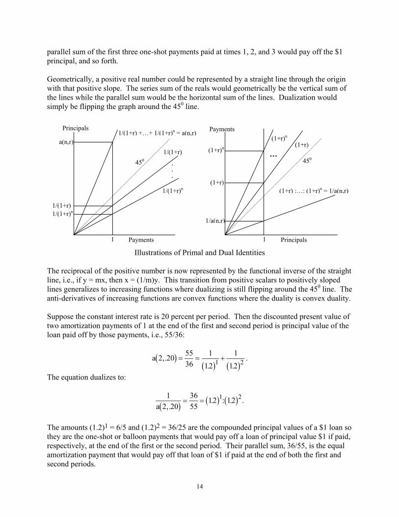
parallel sum of the first three one-shot payments paid at times 1, 2, and 3 would pay off the $1 principal, and so forth. Geometrically, a positive real number could be represented by a straight line through the origin with that positive slope. The series sum of the reals would geometrically be the vertical sum of the lines while the parallel sum would be the horizontal sum of the lines. Dualization would simply be flipping the graph around the 450 line.

Payments Principals

1/a(n,r)

(1+r)

(1+r)n 450 450

1

(1+r) :…: (1+r)n = 1/a(n,r)

…

(1+r)n (1+r)

1

a(n,r)

1/(1+r) 1/(1+r)n

1/(1+r) +…+ 1/(1+r)n = a(n,r)

.

.

.

1/(1+r)n

1/(1+r)

Payments Principals

Illustrations of Primal and Dual Identities The reciprocal of the positive number is now represented by the functional inverse of the straight line, i.e., if y = mx, then x = (1/m)y. This transition from positive scalars to positively sloped lines generalizes to increasing functions where dualizing is still flipping around the 450 line. The anti-derivatives of increasing functions are convex functions where the duality is convex duality. Suppose the constant interest rate is 20 percent per period. Then the discounted present value of two amortization payments of 1 at the end of the first and second period is principal value of the loan paid off by those payments, i.e., 55/36:

( )( ) ( )

a 2 20 5536

1

12

1

121 2,.. .

.= = +

The equation dualizes to:

( ) ( ) ( )12 20

3655

12 121 2a ,.

. : .= = .

The amounts (1.2)1 = 6/5 and (1.2)2 = 36/25 are the compounded principal values of a $1 loan so they are the one-shot or balloon payments that would pay off a loan of principal value $1 if paid, respectively, at the end of the first or the second period. Their parallel sum, 36/55, is the equal amortization payment that would pay off that loan of $1 if paid at the end of both the first and second periods.

14

These facts can be arranged in the following dual format.

Primal Fact: The series sum of the

discounted amortization payments for a loan

is the principal of the loan.

Dual Fact: The parallel sum of the

compounded principals of a loan

is the amortization payment for the loan. The example illustrates some of the substitutions involved in dualizing the interpretation.

series sum ⇔ parallel sum discounting ⇔ compounding principals ⇔ payments

Future Values and Sinking Fund Deposits

Another staple of financial arithmetic is the computation of sinking fund deposits. The compounded future value at time n of n one dollar deposits at times 1,2,…, n is s(n,r), the accumulation of one per period.

( ) ( ) ( ) ( ) ( )( ) .r1r,na1r1r1r1r,ns n12n1n +=+++++++= −− L

Fund Accumulated by One per Period

The discounted values 1/(1+r)n–1,…, 1/(1+r), 1 of a one-dollar fund are the one-shot deposits at times 1,…,n-1, n that would each by itself yield a one-dollar future value for the sinking fund at time n. The parallel sum of these one-shot deposits is the (equal) sinking fund deposit at times 1,…,n-1, n that would yield a one-dollar fund at time n:

( ) ( ) ( ).1:

r11:

r11

r,ns1

11n ++=

−L

Sinking Fund Factor: Payments to Accumulate a Fund of One

The sum of the smooth sinking fund deposits is the harmonic mean of the one-shot deposits. The dual interpretations might be stated as follows.

The series sum of the n compounded one-dollar deposits

is the sinking fund that is accumulated

by the one-dollar deposits.

The parallel sum of the n discounted one-dollar funds

is the deposit that accumulates

to a one-dollar sinking fund.

15

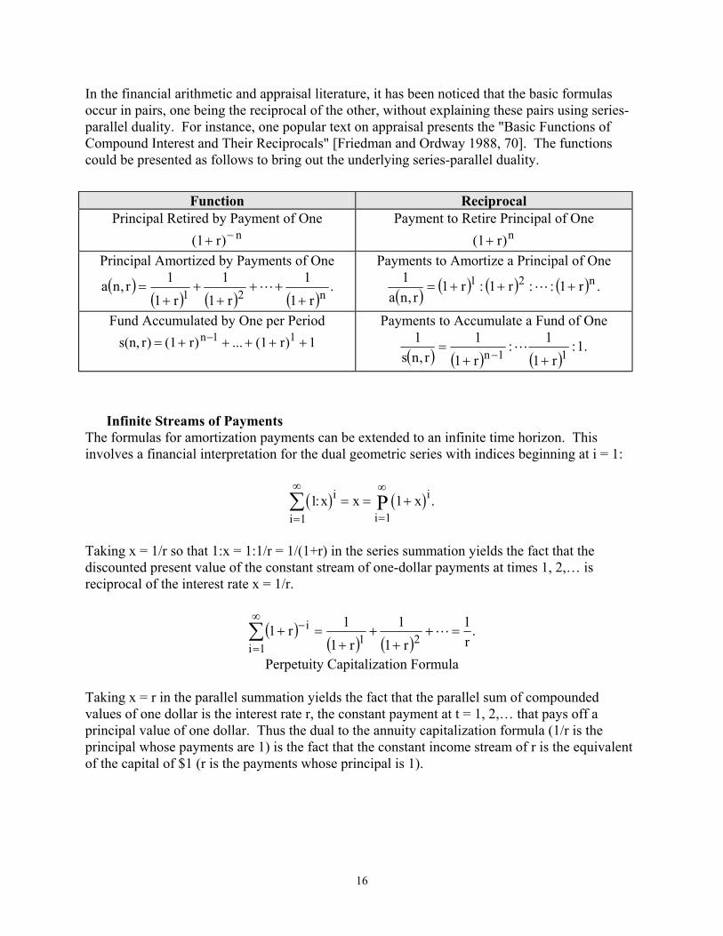
In the financial arithmetic and appraisal literature, it has been noticed that the basic formulas occur in pairs, one being the reciprocal of the other, without explaining these pairs using series-parallel duality. For instance, one popular text on appraisal presents the "Basic Functions of Compound Interest and Their Reciprocals" [Friedman and Ordway 1988, 70]. The functions could be presented as follows to bring out the underlying series-parallel duality.

Function Reciprocal Principal Retired by Payment of One

n)r(1 −+

Payment to Retire Principal of One n)r(1+

Principal Amortized by Payments of One

( )( ) ( ) ( )

.r1

1r1

1r1

1r,nan21 +

+++

++

= L

Payments to Amortize a Principal of One

( ) ( ) ( ) ( ) .r1::r1:r1r,na

1 n21 +++= L

Fund Accumulated by One per Period

1)r(1...)r(1)rs(n, 11n +++++= −

Payments to Accumulate a Fund of One

( ) ( ) ( ).1:

r11:

r11

r,ns1

11n ++=

−L

Infinite Streams of Payments

The formulas for amortization payments can be extended to an infinite time horizon. This involves a financial interpretation for the dual geometric series with indices beginning at i = 1:

( ) ( )1 11 1

: .x x xi

i i

iP=

∞

=

∞∑ = = +

Taking x = 1/r so that 1:x = 1:1/r = 1/(1+r) in the series summation yields the fact that the discounted present value of the constant stream of one-dollar payments at times 1, 2,… is reciprocal of the interest rate x = 1/r.

( )( ) ( )

.r1

r11

r11r1 21

1i

i =++

++

=+∑∞

=

− L

Perpetuity Capitalization Formula

Taking x = r in the parallel summation yields the fact that the parallel sum of compounded values of one dollar is the interest rate r, the constant payment at t = 1, 2,… that pays off a principal value of one dollar. Thus the dual to the annuity capitalization formula (1/r is the principal whose payments are 1) is the fact that the constant income stream of r is the equivalent of the capital of $1 (r is the payments whose principal is 1).

16

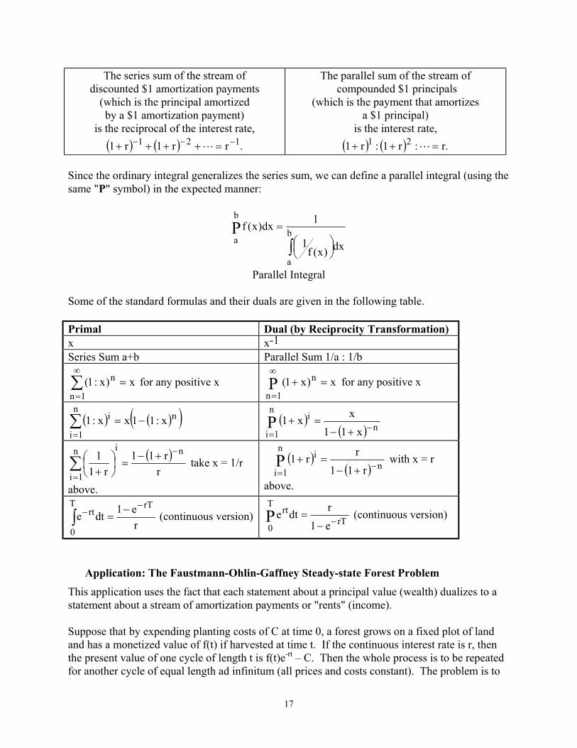
The series sum of the stream of discounted $1 amortization payments

(which is the principal amortized by a $1 amortization payment)

is the reciprocal of the interest rate, ( ) ( ) .rr1r1 121 −−− =++++ L

The parallel sum of the stream of compounded $1 principals

(which is the payment that amortizes a $1 principal)

is the interest rate, ( ) ( ) .r:r1:r1 21 =++ L

Since the ordinary integral generalizes the series sum, we can define a parallel integral (using the same "P" symbol) in the expected manner:

∫

= b

a

b

a dx)x(f1

1dx)x(fP

Parallel Integral Some of the standard formulas and their duals are given in the following table. Primal Dual (by Reciprocity Transformation) x x-1 Series Sum a+b Parallel Sum 1/a : 1/b

x)x:1(1n

n =∑∞

= for any positive x x)x1( n

1nP =+∞

= for any positive x

( ) ( )( )nn

1i

i x:11xx:1 −=∑=

( )( ) n

in

1i x11xx1P −

= +−=+

( )r

r11r1

1 nin

1i

−

=

+−=

+∑ take x = 1/r

above.

( )( ) n

in

1i r11rr1P −

= +−=+ with x = r

above.

re1dte

rTT

0

rt−

− −=∫ (continuous version) rT

rtT

0 e1rdteP −−

= (continuous version)

Application: The Faustmann-Ohlin-Gaffney Steady-state Forest Problem

This application uses the fact that each statement about a principal value (wealth) dualizes to a statement about a stream of amortization payments or "rents" (income). Suppose that by expending planting costs of C at time 0, a forest grows on a fixed plot of land and has a monetized value of f(t) if harvested at time t. If the continuous interest rate is r, then the present value of one cycle of length t is f(t)e-rt – C. Then the whole process is to be repeated for another cycle of equal length ad infinitum (all prices and costs constant). The problem is to

17

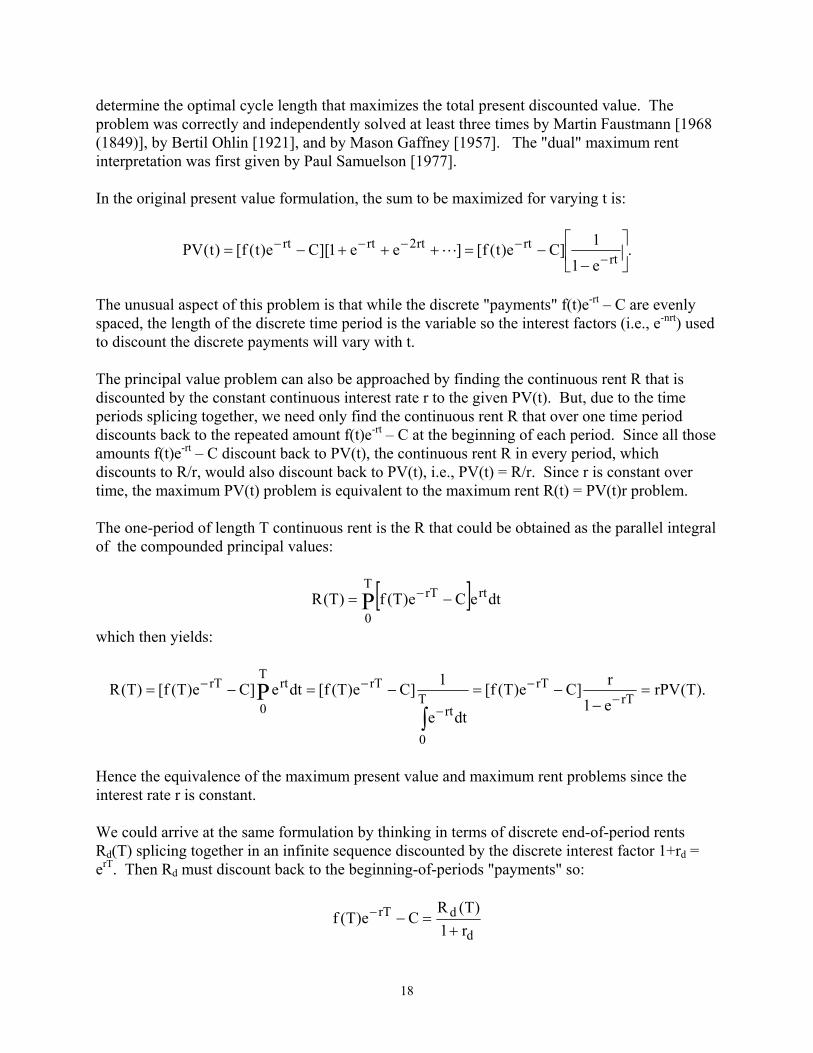
determine the optimal cycle length that maximizes the total present discounted value. The problem was correctly and independently solved at least three times by Martin Faustmann [1968 (1849)], by Bertil Ohlin [1921], and by Mason Gaffney [1957]. The "dual" maximum rent interpretation was first given by Paul Samuelson [1977]. In the original present value formulation, the sum to be maximized for varying t is:

.e11]Ce)t(f[]ee1][Ce)t(f[)t(PV rt

rtrt2rtrt

−−=+++−=

−−−−− L

The unusual aspect of this problem is that while the discrete "payments" f(t)e-rt – C are evenly spaced, the length of the discrete time period is the variable so the interest factors (i.e., e-nrt) used to discount the discrete payments will vary with t. The principal value problem can also be approached by finding the continuous rent R that is discounted by the constant continuous interest rate r to the given PV(t). But, due to the time periods splicing together, we need only find the continuous rent R that over one time period discounts back to the repeated amount f(t)e-rt – C at the beginning of each period. Since all those amounts f(t)e-rt – C discount back to PV(t), the continuous rent R in every period, which discounts to R/r, would also discount back to PV(t), i.e., PV(t) = R/r. Since r is constant over time, the maximum PV(t) problem is equivalent to the maximum rent R(t) = PV(t)r problem. The one-period of length T continuous rent is the R that could be obtained as the parallel integral of the compounded principal values:

[ ] dteCe)T(f)T(R rtrTT

0P −= −

which then yields:

).T(rPVe1r]Ce)T(f[

dte

1]Ce)T(f[dte]Ce)T(f[)T(R rTrT

T

0

rt

rTrtT

0

rT P =−

−=−=−=−

−

−

−−

∫

Hence the equivalence of the maximum present value and maximum rent problems since the interest rate r is constant. We could arrive at the same formulation by thinking in terms of discrete end-of-period rents Rd(T) splicing together in an infinite sequence discounted by the discrete interest factor 1+rd = erT. Then Rd must discount back to the beginning-of-periods "payments" so:

d

drTr1

)T(RCe)T(f

+=−−

18

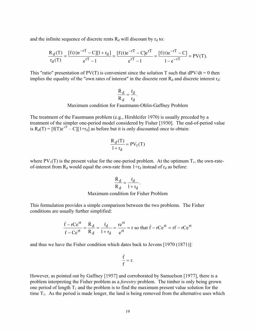
and the infinite sequence of discrete rents Rd will discount by rd to:

).T(PVe1

]Ce)t(f[1e

e]Ce)t(f[1e

]r1][Ce)t(f[)T(r)T(R

rT

rT

rT

rTrT

rTd

rT

d

d =−

−=

−

−=

−

+−=

−

−−−

This "ratio" presentation of PV(T) is convenient since the solution T such that dPV/dt = 0 then implies the equality of the "own rates of interest" in the discrete rent Rd and discrete interest rd:

.rr

RR

d

d

d

d &&=

Maximum condition for Faustmann-Ohlin-Gaffney Problem

The treatment of the Faustmann problem (e.g., Hirshleifer 1970) is usually preceded by a treatment of the simpler one-period model considered by Fisher [1930]. The end-of-period value is Rd(T) = [f(T)e-rT – C][1+rd] as before but it is only discounted once to obtain:

)T(PVr1

)T(R1

d

d =+

where PV1(T) is the present value for the one-period problem. At the optimum T1, the own-rate-of-interest from Rd would equal the own-rate from 1+rd instead of rd as before:

.r1

rRR

d

d

d

d+

=&&

Maximum condition for Fisher Problem

This formulation provides a simple comparison between the two problems. The Fisher conditions are usually further simplified:

rtrtrt

rt

d

d

d

drt

rtrCerfrCefthatsor

ere

r1r

RR

CefrCef

−=−==+

==−

− &&&&

and thus we have the Fisher condition which dates back to Jevons [1970 (1871)]:

.rff

=&

However, as pointed out by Gaffney [1957] and corroborated by Samuelson [1977], there is a problem interpreting the Fisher problem as a forestry problem. The timber is only being grown one period of length T1 and the problem is to find the maximum present value solution for the time T1. As the period is made longer, the land is being removed from the alternative uses which

19

will have some opportunity cost that does not figure in the problem. Hence to awkwardly interpret the Fisher problem as a forestry problem, we would have to assume that the land had no other uses as if growing the timber once would "salt" or ruin the land for any later uses. Summary Fisher 1-Period Problem Faustmann-Ohlin-Gaffney Problem Statement of Problem

d

d1 r1

)T(R)T(PVMax

+=

d

dr

)T(R)T(PVMax =

Max Conditions

d

d

d

dr1

rRR

+=

&&

where .rr1

r

d

d =+&

d

d

d

drr

RR &&

=

where ( )K&

+++= −− rt2rt

d

d ee1rrr

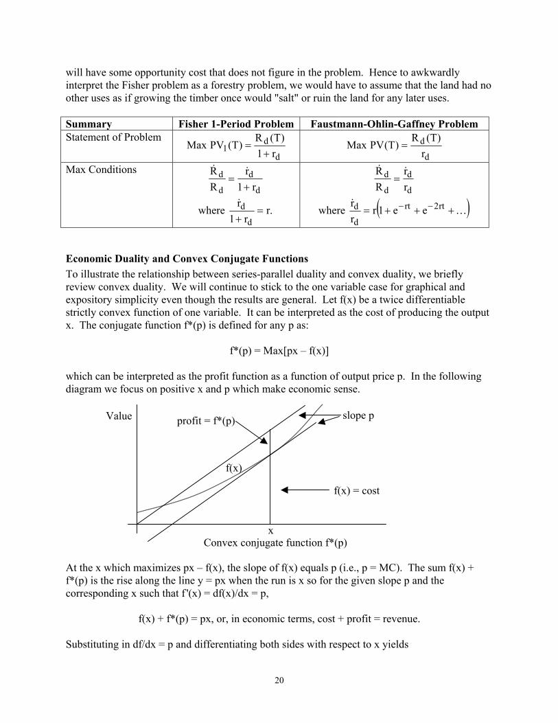
Economic Duality and Convex Conjugate Functions To illustrate the relationship between series-parallel duality and convex duality, we briefly review convex duality. We will continue to stick to the one variable case for graphical and expository simplicity even though the results are general. Let f(x) be a twice differentiable strictly convex function of one variable. It can be interpreted as the cost of producing the output x. The conjugate function f*(p) is defined for any p as:

f*(p) = Max[px – f(x)] which can be interpreted as the profit function as a function of output price p. In the following diagram we focus on positive x and p which make economic sense.

profit = f*(p)

f(x) = cost

slope p

f(x)

Value

x Convex conjugate function f*(p)

At the x which maximizes px – f(x), the slope of f(x) equals p (i.e., p = MC). The sum f(x) + f*(p) is the rise along the line y = px when the run is x so for the given slope p and the corresponding x such that f '(x) = df(x)/dx = p,

f(x) + f*(p) = px, or, in economic terms, cost + profit = revenue. Substituting in df/dx = p and differentiating both sides with respect to x yields

20

df/dx + (df*/dp) d2f/dx2 = df/dx + xd2f/dx2.

Subtracting df/dx from each side and canceling the second derivative (which is positive by strict convexity) yields

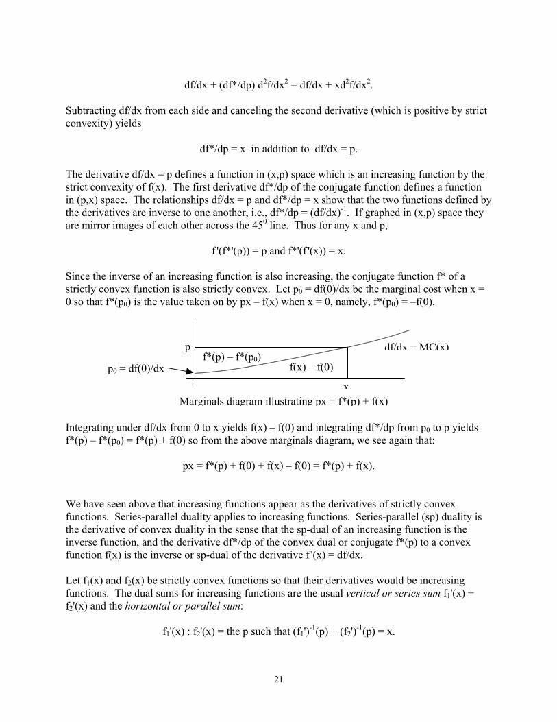
df*/dp = x in addition to df/dx = p. The derivative df/dx = p defines a function in (x,p) space which is an increasing function by the strict convexity of f(x). The first derivative df*/dp of the conjugate function defines a function in (p,x) space. The relationships df/dx = p and df*/dp = x show that the two functions defined by the derivatives are inverse to one another, i.e., df*/dp = (df/dx)-1. If graphed in (x,p) space they are mirror images of each other across the 450 line. Thus for any x and p,

f '(f*'(p)) = p and f*'(f '(x)) = x. Since the inverse of an increasing function is also increasing, the conjugate function f* of a strictly convex function is also strictly convex. Let p0 = df(0)/dx be the marginal cost when x = 0 so that f*(p0) is the value taken on by px – f(x) when x = 0, namely, f*(p0) = –f(0).

f*(p) – f*(p0) p0 = df(0)/dx f(x) – f(0)

df/dx = MC(x)p

x

Marginals diagram illustrating px = f*(p) + f(x) Integrating under df/dx from 0 to x yields f(x) – f(0) and integrating df*/dp from p0 to p yields f*(p) – f*(p0) = f*(p) + f(0) so from the above marginals diagram, we see again that:

px = f*(p) + f(0) + f(x) – f(0) = f*(p) + f(x). We have seen above that increasing functions appear as the derivatives of strictly convex functions. Series-parallel duality applies to increasing functions. Series-parallel (sp) duality is the derivative of convex duality in the sense that the sp-dual of an increasing function is the inverse function, and the derivative df*/dp of the convex dual or conjugate f*(p) to a convex function f(x) is the inverse or sp-dual of the derivative f '(x) = df/dx. Let f1(x) and f2(x) be strictly convex functions so that their derivatives would be increasing functions. The dual sums for increasing functions are the usual vertical or series sum f1'(x) + f2'(x) and the horizontal or parallel sum:

f1'(x) : f2'(x) = the p such that (f1')-1(p) + (f2')-1(p) = x.

21

The parallel sum of positive scalars x and y is [x:y]-1 = (1/x)+(1/y) is dual to the usual sum x+y, and the parallel sum of increasing functions can be written in an analogous way:

[f1'(x) : f2'(x)]-1(p) = [(f1')-1(p) + (f2')-1(p)]. The duality relationship carries over, mutatis mutandis, to the duality of series-parallel combinations of increasing functions. For instance, the dual of the function

(f1')-1(p) + (f2')-1(p) would be f1'(x):f2'(x) and, indeed, we see from the definition of the parallel sum of functions that the two are inverses of one another. Continuing on the theme that convex duality and series-parallel duality are related as a (convex) function is to its derivative, we can expect that there would be two sums of convex functions whose derivatives would be the corresponding series and parallel sums of the derivatives. This is trivial for the series sums. The ordinary (series) sum of convex functions is convex and its derivative is the series or vertical sum of the derivatives, i.e.,

d[f1(x)+f2(x)]/dx = f1'(x) + f2'(x). There is also a "parallel sum" of convex functions and it has an economic interpretation in our example of cost functions. Suppose that the firm has two plants and that we are only given the two (again strictly convex and differentiable) cost functions f1(x) and f2(x) for the plants. The overall cost function could then be defined as the infimal convolution [Rockafellar 1970, 34] of the two functions:

)].x(f)xx(f[)x(f)x(f 2221x

21 inf2

+−=⊕

The infimum would (by strict convexity) occur at the g(x) = x2 where f1'(x-g(x)) = f2'(g(x)) and that common value p (the same marginal cost in each plant) is the p such that:

(f1')-1(p) + (f2')-1(p) = x-g(x) + g(x) = x. The derivative of the infimal convolution is:

p))x(gx('f))x(g('f'g))x(g('f)'g1))(x(g('f

'g))x(g('f)'g1))(x(gx('fdx

))]x(g(f))x(gx(f[ddx

)]x(f)x(f[d

1222

212121

=−==+−=

+−−=+−

=⊕

where the p is such that: (f1')-1(p) + (f2')-1(p) = x-g(x) + g(x) = x which is precisely the p that is the value of f1'(x) : f2'(x). Hence the derivative of the infimal convolution is the parallel sum of the derivatives:

22

).x('f:)x('fdx

)]x(f)x(f[d21

21 =⊕

On the economic interpretation, the overall marginal cost is the parallel sum of the marginal costs for the separate plants. It remains to show that the infimal convolution and ordinary sum of convex functions are dual operations. Given the two convex functions f1*(p) and f2*(p), the dual to their sum is:

(f1* + f2*)*(x) = Max[px – f1*(p) – f2*(p)] where the maximum occurs at the p where x = df1*(p)/dp + df2*(p)/dp = (f1')-1(p) + (f2')-1(p) The result to be proven is that the value of this function at that x is the same as the value of the infimal convolution at that x:

))]x(g(f))x(gx(f[)x(f)x(f 2121 +−=⊕ for the previously defined g(x) = x2 such that f1'(x-g(x)) = f2'(g(x)) and that common value p is the p such that: (f1')-1(p) + (f2')-1(p) = x-g(x) + g(x) = x. Hence we have:

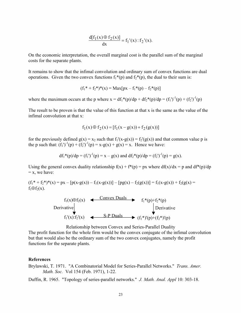
df1*(p)/dp = (f1')-1(p) = x – g(x) and df2*(p)/dp = (f2')-1(p) = g(x). Using the general convex duality relationship f(x) + f*(p) = px where df(x)/dx = p and df*(p)/dp = x, we have: (f1* + f2*)*(x) = px – [p(x-g(x)) – f1(x-g(x))] – [pg(x) – f2(g(x))] = f1(x-g(x)) + f2(g(x) = f1⊕f2(x).

f1(x)⊕f2(x) f1*(p)+f2*(p)

f1'(x):f2'(x) (f1*)'(p)+(f2*)'(p)

Derivative

S-P Duals

Convex Duals Derivative

Relationship between Convex and Series-Parallel Duality The profit function for the whole firm would be the convex conjugate of the infimal convolution but that would also be the ordinary sum of the two convex conjugates, namely the profit functions for the separate plants.

References Brylawski, T. 1971. "A Combinatorial Model for Series-Parallel Networks." Trans. Amer.

Math. Soc. Vol 154 (Feb. 1971), 1-22.

Duffin, R. 1965. "Topology of series-parallel networks." J. Math. Anal. Appl 10: 303-18.

23

Duffin, R. 1975. "Electrical Network Models." In Studies in Graph Theory, Part I (D. R. Fulkerson, ed.), Math. Assn. of America: 94-138.

Faustmann, Martin 1968 (1849). On the Determination of the Value Which Forest Land and Immature Stands Possess for Forestry. In Martin Faustmann and the Evolution of Discounted Cash Flow: Oxford Institute Paper 42. Ed. by M. Gane.

Fisher, Irving 1930. The Theory of Interest. New York: Macmillan.

Friedman, Jack P. and Nicholas Ordway 1988. Income Property Appraisal and Analysis. Englewood Cliffs: Prentice Hall.

Gaffney, Mason 1957. Concepts of financial maturity of timber and other assets. In Agricultural Economics Information Series 62. Raleigh NC: North Carolina State College.

Hirshleifer, Jack 1970. Investment, Interest, and Capital. Englewood Cliffs: Prentice-Hall.

Jevons, W. Stanley 1970 (1871). The Theory of Political Economy. Harmondsworth: Penguin Books.

Lehman, Alfred. 1962. "Problem 60-5-A resistor network inequality." SIAM Review 4: 150-55.

MacMahon, Percy A. 1881. "Yoke-Chains and Multipartite Compositions in connexion with the Analytical Forms called 'Trees' ." Proc. London Math. Soc. 22: 330-46.

MacMahon, Percy A. 1892. "The Combinations of Resistances." The Electrician 28, 601-2.

MacMahon, Percy A. 1978. Collected Papers: Volume I, Combinatorics. Edited by George E. Andrews. Cambridge, Mass.: MIT Press.

Ohlin, Bertil 1921. Till Fragen om skogarnas omloppstid. In Ekonomisk Tidskrift, "Festschrift to Knut Wicksell".

Riordan, J., and C. Shannon. 1942. "The Number of Two-Terminal Series-Parallel Networks." J. Math. Phys. of MIT 21: 83-93.

Rockafellar, R. T. 1970. Convex Analysis. Princeton: Princeton University Press.

Samuelson, Paul A. 1977. Economics of Forestry in an Evolving Society. In The Collected Scientific Papers of Paul A. Samuelson: Volume IV. Ed. by H. Nagatani and K. Crowley. Cambridge: MIT Press: 146-72.

Scudder Funds 1988. News from the Scudder Funds. (Spring). Boston, Mass.

24