Introduction to Pseudopotentials and Electronic Structure

Philip B. Allen Stony Brook University

Nov. 3, 2014 Brookhaven National Laboratory

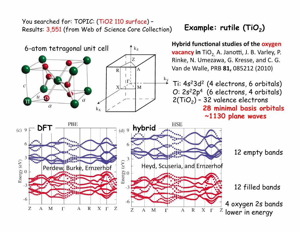
You searched for: TOPIC: (TiO2 110 surface) – Results: 3,551 (from Web of Science Core Collection)

Ti: 4s23d2 (4 electrons, 6 orbitals)

O: 2s22p4 (6 electrons, 4 orbitals)

2(TiO2) – 32 valence electrons 28 minimal basis orbitals ~1130 plane waves

12 filled bands

12 empty bands

Hybrid  func,onal  studies  of  the  oxygen  vacancy  in  TiO2,  A.  Jano-,  J.  B.  Varley,  P.  Rinke,  N.  Umezawa,  G.  Kresse,  and  C.  G.  Van  de  Walle,  PRB  81,  085212  (2010)  

Heyd,  Scuseria,  and  Ernzerhof  Perdew,  Burke,  Ernzerhof  

4 oxygen 2s bands lower in energy

6-atom tetragonal unit cell

Example: rutile (TiO2)

DFT hybrid

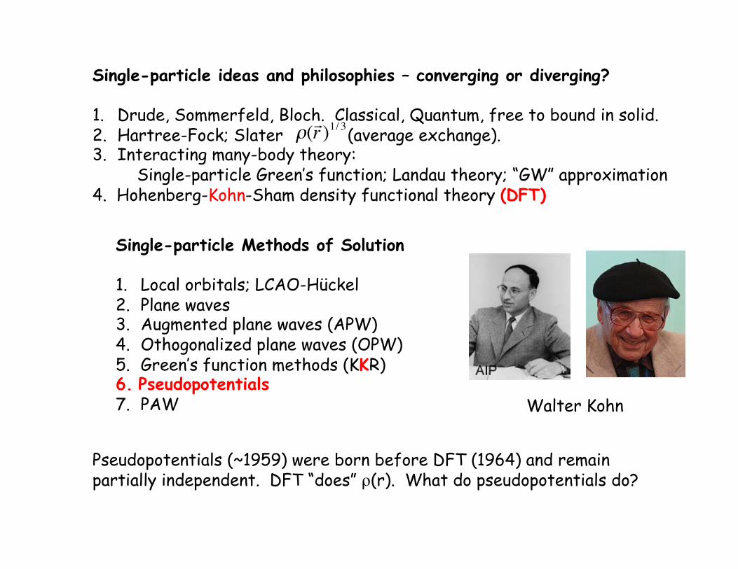
Single-particle ideas and philosophies – converging or diverging?

1.  Drude, Sommerfeld, Bloch. Classical, Quantum, free to bound in solid. 2.  Hartree-Fock; Slater (average exchange). 3.  Interacting many-body theory: Single-particle Green’s function; Landau theory; “GW” approximation 4. Hohenberg-Kohn-Sham density functional theory (DFT)

€

ρ(! r )1/ 3

Single-particle Methods of Solution

1.  Local orbitals; LCAO-Hückel 2.  Plane waves 3.  Augmented plane waves (APW) 4.  Othogonalized plane waves (OPW) 5.  Green’s function methods (KKR) 6.  Pseudopotentials 7.  PAW Walter Kohn

Pseudopotentials (~1959) were born before DFT (1964) and remain partially independent. DFT “does” ρ(r). What do pseudopotentials do?

€

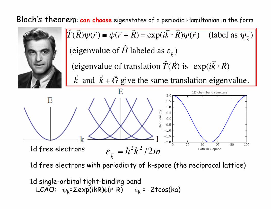
ˆ T (! R )ψ(! r ) ≡ψ(! r +

! R ) = exp(i

! k ⋅! R )ψ(! r ) (label as ψ ! k )

(eigenvalue of ˆ H labeled as ε ! k )

(eigenvalue of translation ˆ T (! R ) is exp(i

! k ⋅! R )

! k and

! k +! G give the same translation eigenvalue.

Bloch’s theorem: can choose eigenstates of a periodic Hamiltonian in the form

1d free electrons

1d free electrons with periodicity of k-space (the reciprocal lattice)

1d single-orbital tight-binding band LCAO: ψk=Σexp(ikR)φ(r-R) εk = -2tcos(ka)

€

ε ! k

= "2k 2 /2m

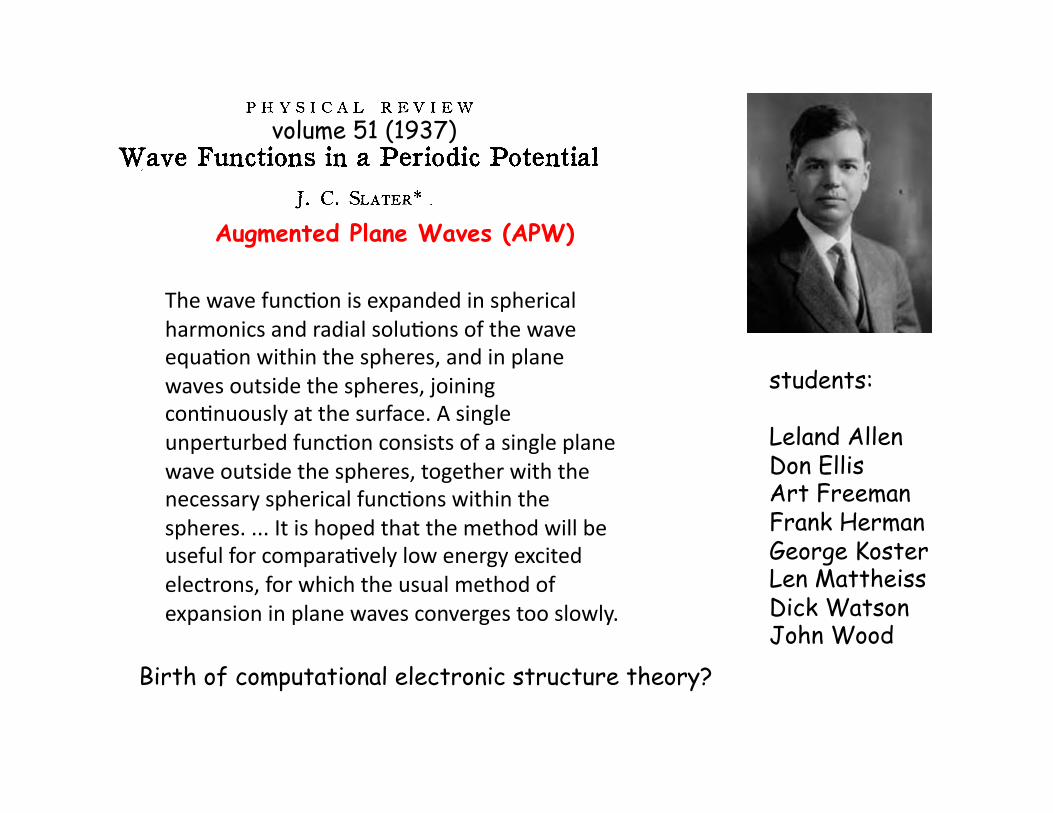
volume 51 (1937)

The  wave  funcPon  is  expanded  in  spherical  harmonics  and  radial  soluPons  of  the  wave  equaPon  within  the  spheres,  and  in  plane  waves  outside  the  spheres,  joining  conPnuously  at  the  surface.  A  single  unperturbed  funcPon  consists  of  a  single  plane  wave  outside  the  spheres,  together  with  the  necessary  spherical  funcPons  within  the  spheres.  ...  It  is  hoped  that  the  method  will  be  useful  for  comparaPvely  low  energy  excited  electrons,  for  which  the  usual  method  of  expansion  in  plane  waves  converges  too  slowly.  

Augmented Plane Waves (APW)

students:

Leland Allen Don Ellis Art Freeman Frank Herman George Koster Len Mattheiss Dick Watson John Wood

Birth of computational electronic structure theory?

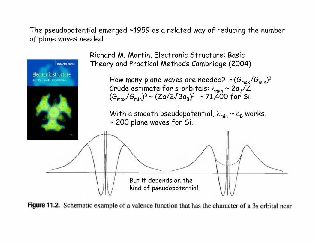
Richard M. Martin, Electronic Structure: Basic Theory and Practical Methods Cambridge (2004)

How many plane waves are needed? ~(Gmax/Gmin)3

Crude estimate for s-orbitals: λmin ~ 2aB/Z (Gmax/Gmin)3 ~ (Za/2√3aB)3 ~ 71,400 for Si.

With a smooth pseudopotential, λmin ~ aB works. ~ 200 plane waves for Si.

The pseudopotential emerged ~1959 as a related way of reducing the number of plane waves needed.

But it depends on the kind of pseudopotential.

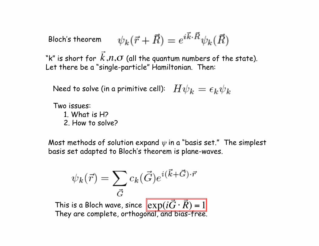
Bloch’s theorem

“k” is short for (all the quantum numbers of the state). Let there be a “single-particle” Hamiltonian. Then:

€

! k ,n,σ

Most methods of solution expand ψ in a “basis set.” The simplest basis set adapted to Bloch’s theorem is plane-waves.

This is a Bloch wave, since They are complete, orthogonal, and bias-free.

€

exp(i! G ⋅! R ) =1

Need to solve (in a primitive cell):

Two issues: 1. What is H? 2. How to solve?

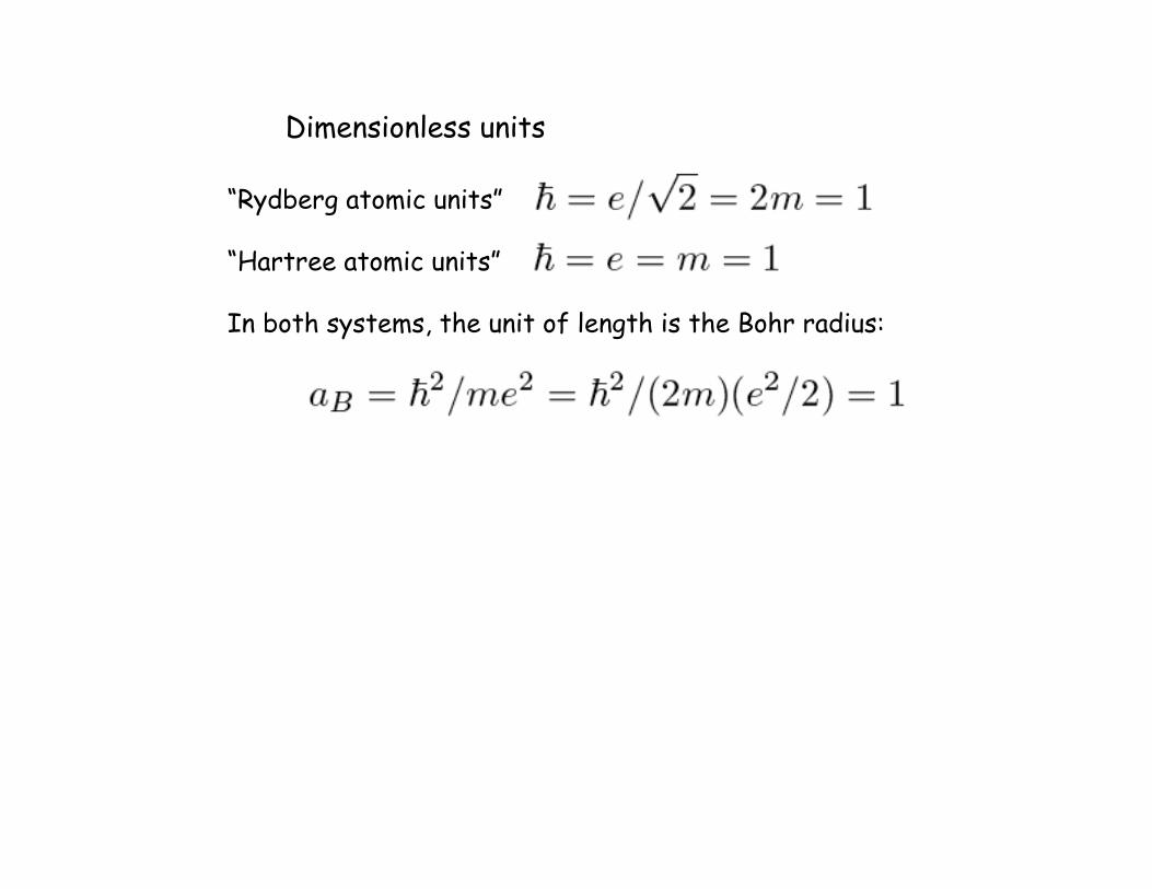
Dimensionless units

“Rydberg atomic units”

“Hartree atomic units”

In both systems, the unit of length is the Bohr radius:

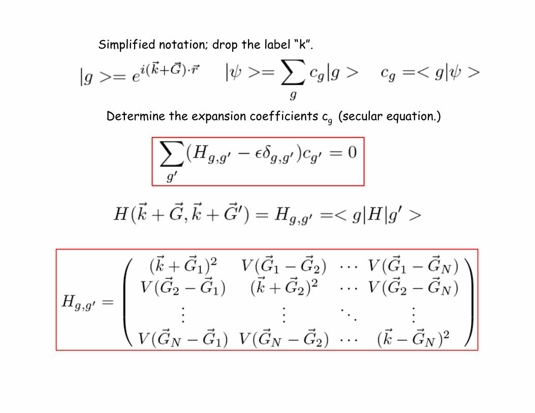
Simplified notation; drop the label “k”.

Determine the expansion coefficients cg (secular equation.)

€

ψ =n=1

∞

∑ αn n

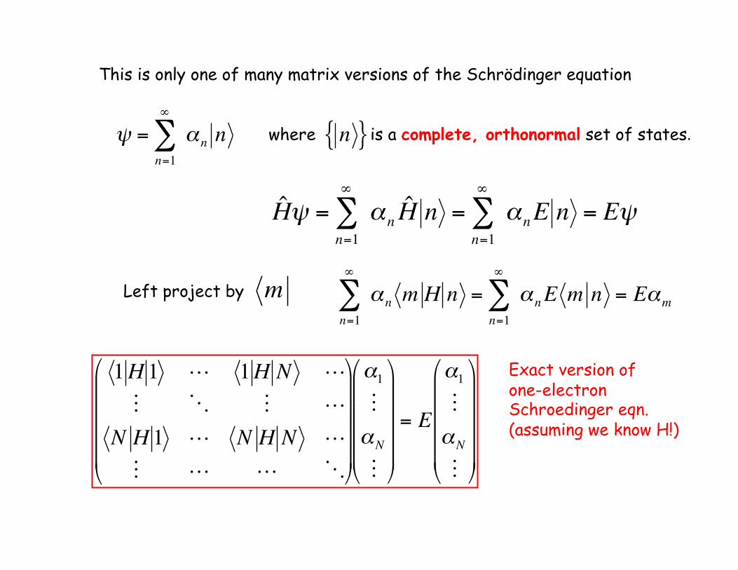
This is only one of many matrix versions of the Schrödinger equation

€

n{ }where is a complete, orthonormal set of states.  

€

ˆ H ψ =n=1

∞

∑ αnˆ H n =

n=1

∞

∑ αn E n = Eψ

Left project by    

€

m

€

n=1

∞

∑ αn m H n =n=1

∞

∑ αnE m n = Eαm

€

1H 1 ! 1H N !" # " !

N H 1 ! N H N !" ! ! #

⎛

⎝

⎜ ⎜ ⎜ ⎜

⎞

⎠

⎟ ⎟ ⎟ ⎟

α1"αN

"

⎛

⎝

⎜ ⎜ ⎜ ⎜

⎞

⎠

⎟ ⎟ ⎟ ⎟

= E

α1"αN

"

⎛

⎝

⎜ ⎜ ⎜ ⎜

⎞

⎠

⎟ ⎟ ⎟ ⎟

Exact version of one-electron Schroedinger eqn. (assuming we know H!)

€

ψ =n=1

N

∑ αn n

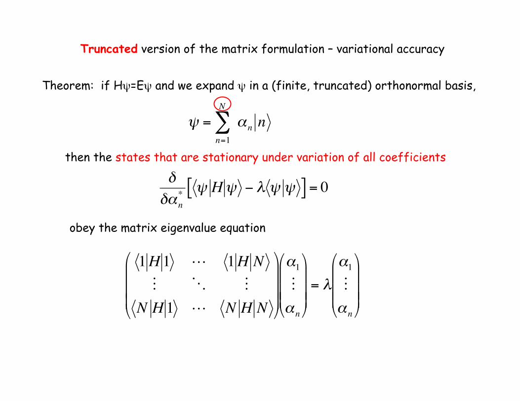
Theorem: if Hψ=Eψ and we expand ψ in a (finite, truncated) orthonormal basis,

€

δδαn

* ψ Hψ − λ ψ ψ[ ] = 0

then the states that are stationary under variation of all coefficients

obey the matrix eigenvalue equation

€

1H 1 ! 1H N" # "

N H 1 ! N H N

⎛

⎝

⎜ ⎜ ⎜

⎞

⎠

⎟ ⎟ ⎟

α1"αn

⎛

⎝

⎜ ⎜ ⎜

⎞

⎠

⎟ ⎟ ⎟

= λ

α1"αn

⎛

⎝

⎜ ⎜ ⎜

⎞

⎠

⎟ ⎟ ⎟

Truncated version of the matrix formulation – variational accuracy

€

ˆ H

α1

!αN

!

⎛

⎝

⎜ ⎜ ⎜ ⎜

⎞

⎠

⎟ ⎟ ⎟ ⎟

= E ˆ S

α1

!αN

!

⎛

⎝

⎜ ⎜ ⎜ ⎜

⎞

⎠

⎟ ⎟ ⎟ ⎟

€

ˆ H =

1 H 1 ! 1 H N !" # " !

N H 1 ! N H N !" ! ! #

⎛

⎝

⎜ ⎜ ⎜ ⎜

⎞

⎠

⎟ ⎟ ⎟ ⎟

€

ˆ S =

1 1 ! 1 N !" # " !

N 1 ! N N !" ! ! #

⎛

⎝

⎜ ⎜ ⎜ ⎜

⎞

⎠

⎟ ⎟ ⎟ ⎟

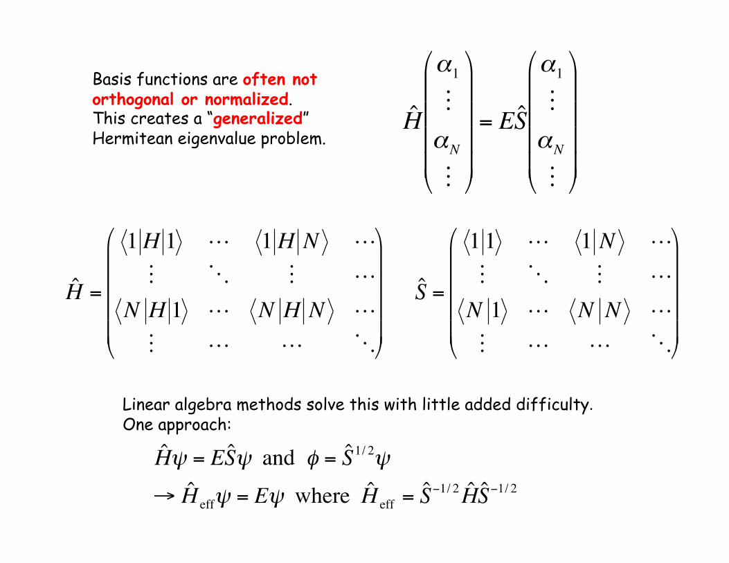
Basis functions are often not orthogonal or normalized. This creates a “generalized” Hermitean eigenvalue problem.

Linear algebra methods solve this with little added difficulty.  One approach:

€

ˆ H ψ = E ˆ S ψ and φ = ˆ S 1/ 2ψ

→ ˆ H effψ = Eψ where ˆ H eff = ˆ S −1/ 2 ˆ H ̂ S −1/ 2

€

ˆ H (E)

α1

!αN

!

⎛

⎝

⎜ ⎜ ⎜ ⎜

⎞

⎠

⎟ ⎟ ⎟ ⎟

= E ˆ S (E)

α1

!αN

!

⎛

⎝

⎜ ⎜ ⎜ ⎜

⎞

⎠

⎟ ⎟ ⎟ ⎟

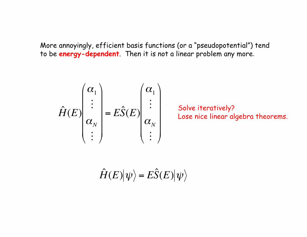
More annoyingly, efficient basis functions (or a “pseudopotential”) tend to be energy-dependent. Then it is not a linear problem any more.  

€

ˆ H (E)ψ = E ˆ S (E)ψ

Solve iteratively? Lose nice linear algebra theorems.

€

ˆ H (E)ψ = E ˆ S (E)ψ

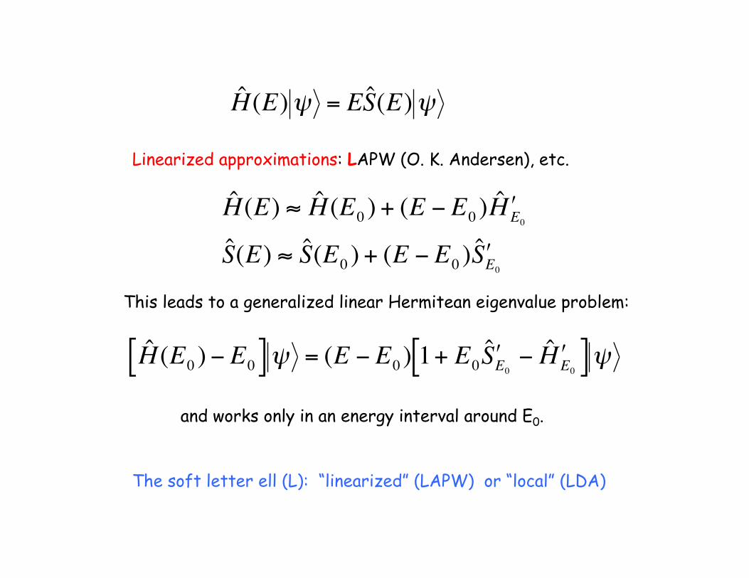
Linearized approximations: LAPW (O. K. Andersen), etc.

€

ˆ H (E0 ) − E0[ ]ψ = (E − E0 ) 1+ E0ˆ ʹ′ S E0

− ˆ ʹ′ H E0[ ]ψ€

ˆ H (E) ≈ ˆ H (E0 ) + (E − E0 ) ˆ ʹ′ H E0

ˆ S (E) ≈ ˆ S (E0 ) + (E − E0 ) ˆ ʹ′ S E0

This leads to a generalized linear Hermitean eigenvalue problem:

and works only in an energy interval around E0.

The soft letter ell (L): “linearized” (LAPW) or “local” (LDA)

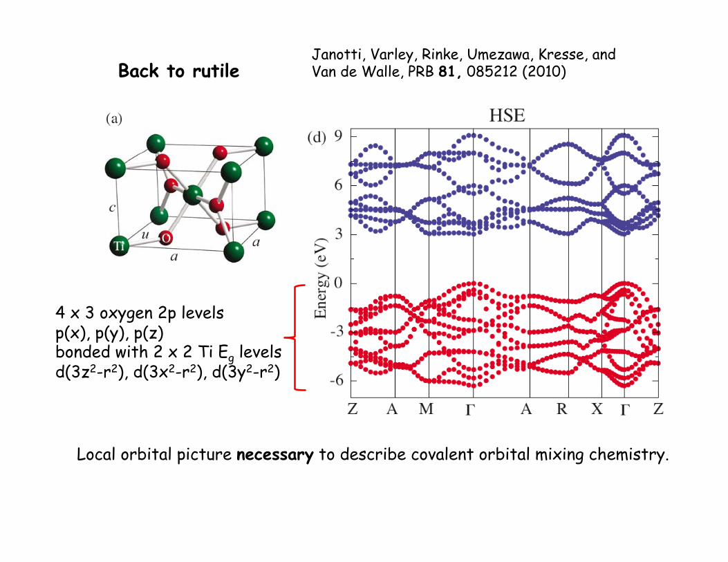
Back to rutile

4 x 3 oxygen 2p levels p(x), p(y), p(z) bonded with 2 x 2 Ti Eg levels d(3z2-r2), d(3x2-r2), d(3y2-r2)

Janotti, Varley, Rinke, Umezawa, Kresse, and Van de Walle, PRB 81, 085212 (2010)

Local orbital picture necessary to describe covalent orbital mixing chemistry.

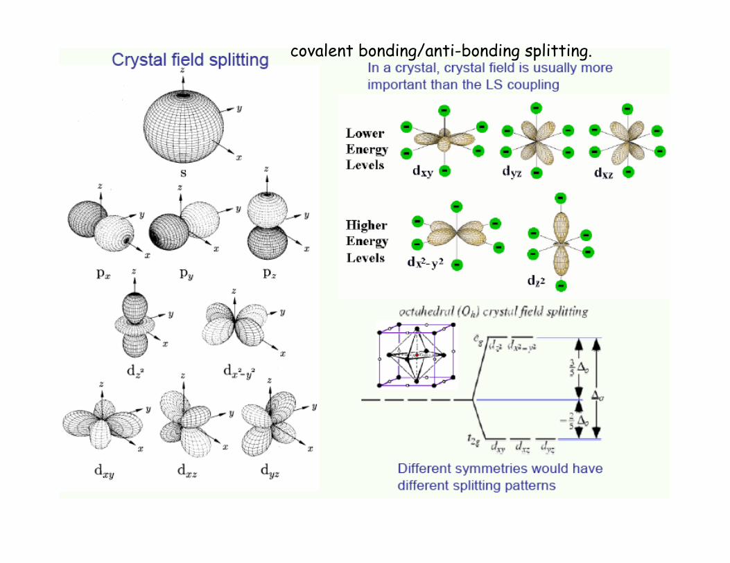
covalent bonding/anti-bonding splitting.

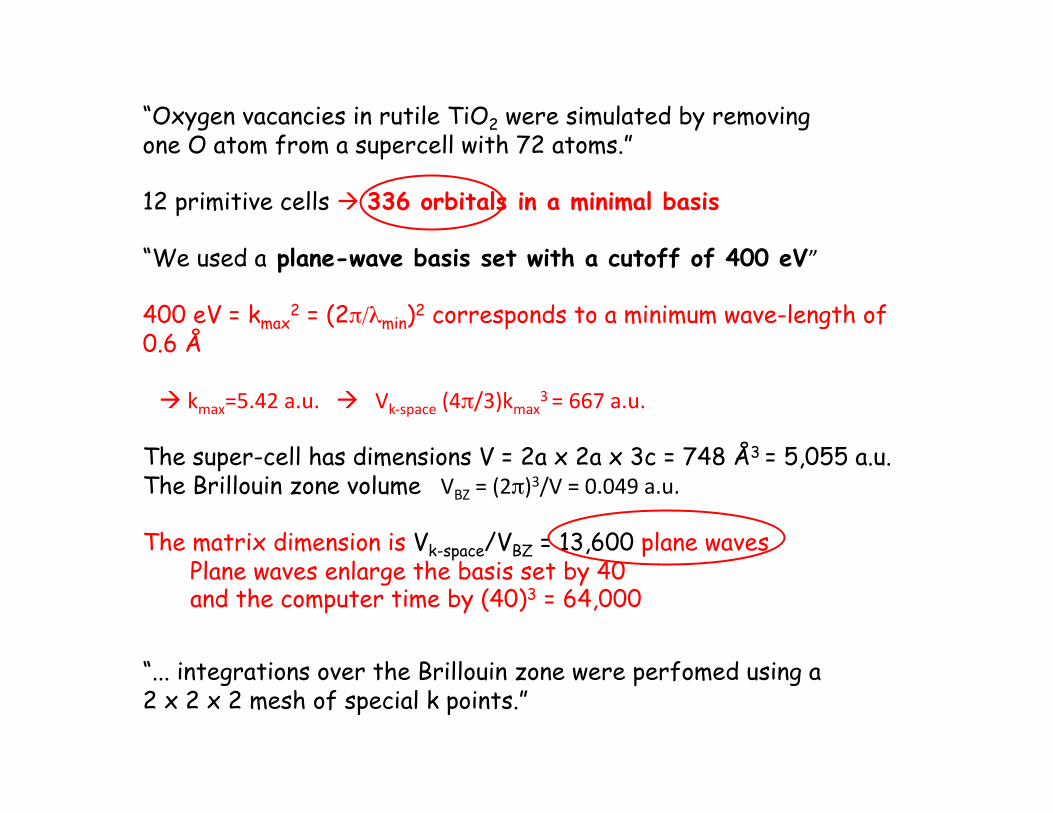
“Oxygen vacancies in rutile TiO2 were simulated by removing one O atom from a supercell with 72 atoms.”

12 primitive cells ! 336 orbitals in a minimal basis

“We used a plane-wave basis set with a cutoff of 400 eV”    

400 eV = kmax2 = (2π/λmin)2 corresponds to a minimum wave-length of

0.6 Å

     !  kmax=5.42  a.u.      !      Vk-­‐space  (4π/3)kmax3  =  667  a.u.  

The super-cell has dimensions V = 2a x 2a x 3c = 748 Å3 = 5,055 a.u. The Brillouin zone volume  VBZ  =  (2π)3/V  =  0.049  a.u.  

The matrix dimension is Vk-space/VBZ = 13,600 plane waves Plane waves enlarge the basis set by 40 and the computer time by (40)3 = 64,000

“... integrations over the Brillouin zone were perfomed using a 2 x 2 x 2 mesh of special k points.”

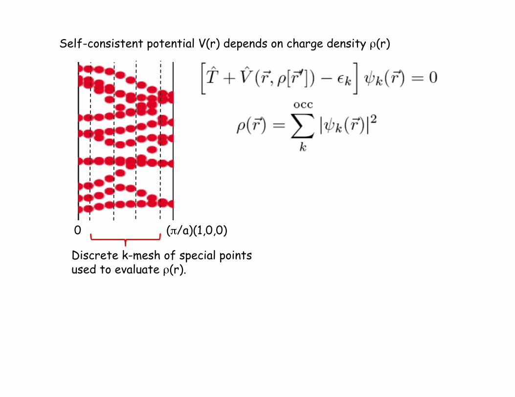
0 (π/a)(1,0,0)

Self-consistent potential V(r) depends on charge density ρ(r)

Discrete k-mesh of special points used to evaluate ρ(r).

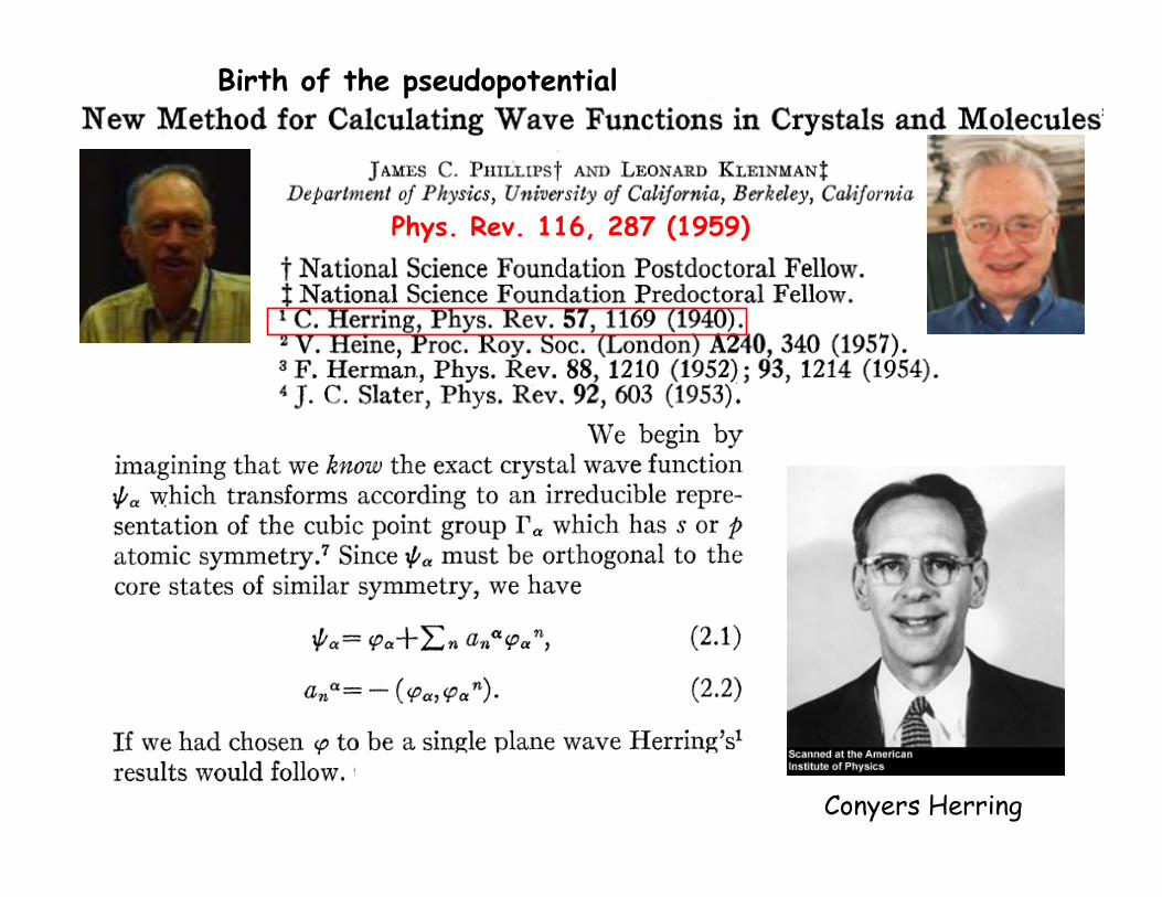
Phys. Rev. 116, 287 (1959)

Conyers Herring

Birth of the pseudopotential

€

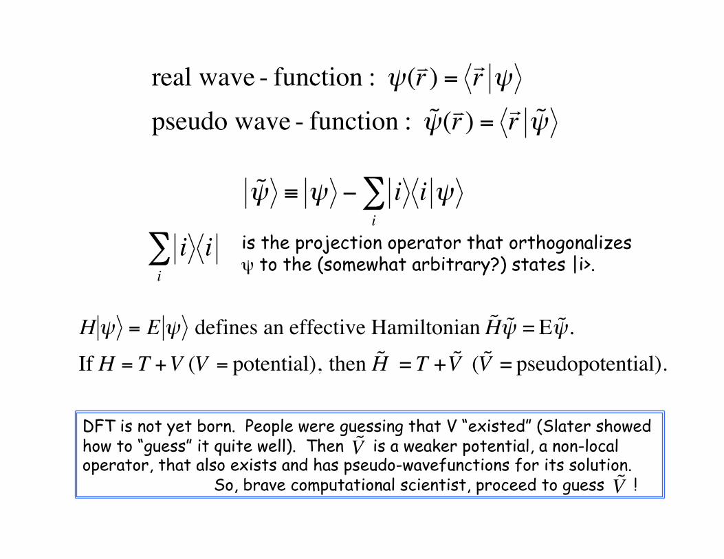
˜ ψ ≡ ψ − i i ψi∑

€

real wave - function : ψ(! r ) =" r ψ

pseudo wave - function : ˜ ψ (! r ) =" r ˜ ψ

€

i ii∑ is the projection operator that orthogonalizes

ψ to the (somewhat arbitrary?) states |i>.

€

Hψ = E ψ defines an effective Hamiltonian ˜ H ˜ ψ = E ˜ ψ .If H = T +V (V = potential), then ˜ H = T + ˜ V ( ˜ V = pseudopotential).

DFT is not yet born. People were guessing that V “existed” (Slater showed how to “guess” it quite well). Then is a weaker potential, a non-local operator, that also exists and has pseudo-wavefunctions for its solution. So, brave computational scientist, proceed to guess !

€

˜ V

€

˜ V

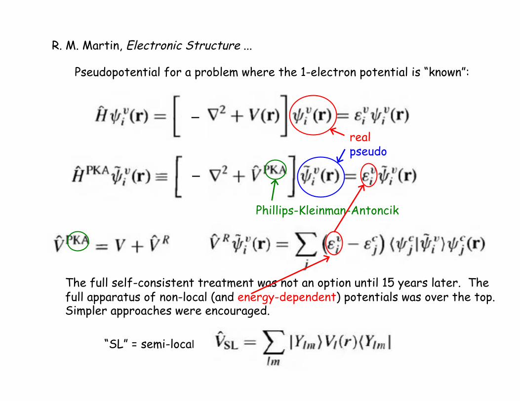
Pseudopotential for a problem where the 1-electron potential is “known”:

   –          

   –          

real pseudo

Phillips-Kleinman-Antoncik

The full self-consistent treatment was not an option until 15 years later. The full apparatus of non-local (and energy-dependent) potentials was over the top. Simpler approaches were encouraged.

R. M. Martin, Electronic Structure ...

“SL” = semi-local  

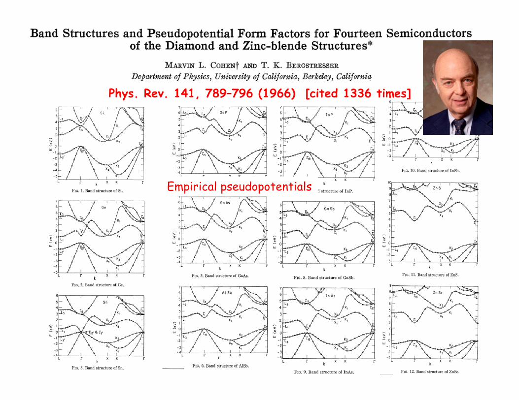
Phys. Rev. 141, 789–796 (1966) [cited 1336 times]

Empirical pseudopotentials

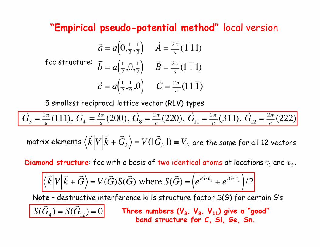
“Empirical pseudo-potential method” local version

fcc structure:    

€

! a = a 0, 12 , 1

2( ) ! A = 2π

a (1 11)! b = a 1

2 ,0, 12( )

! B = 2π

a (11 1)! c = a 1

2 , 12 ,0( )

! C = 2π

a (111 )

€

! G 3 = 2π

a (111), ! G 4 = 2π

a (200), ! G 8 = 2π

a (220), ! G 11 = 2π

a (311), ! G 12 = 2π

a (222)5 smallest reciprocal lattice vector (RLV) types

€

! k V! k +! G 3 = V (|

! G 3 |) ≡V3matrix elements are the same for all 12 vectors

Diamond structure: fcc with a basis of two identical atoms at locations τ1 and τ2..

€

! k V! k +! G = V (

! G )S(

! G ) where S(

! G ) = ei

! G ⋅ ! τ 1 + ei

! G ⋅ ! τ 2( ) /2

€

S(! G 4 ) = S(

! G 12) = 0 Three numbers (V3, V8, V11) give a “good”

band structure for C, Si, Ge, Sn.

Note – destructive interference kills structure factor S(G) for certain G’s.

opti

cal r

efle

ctiv

ity

ħω (eV)

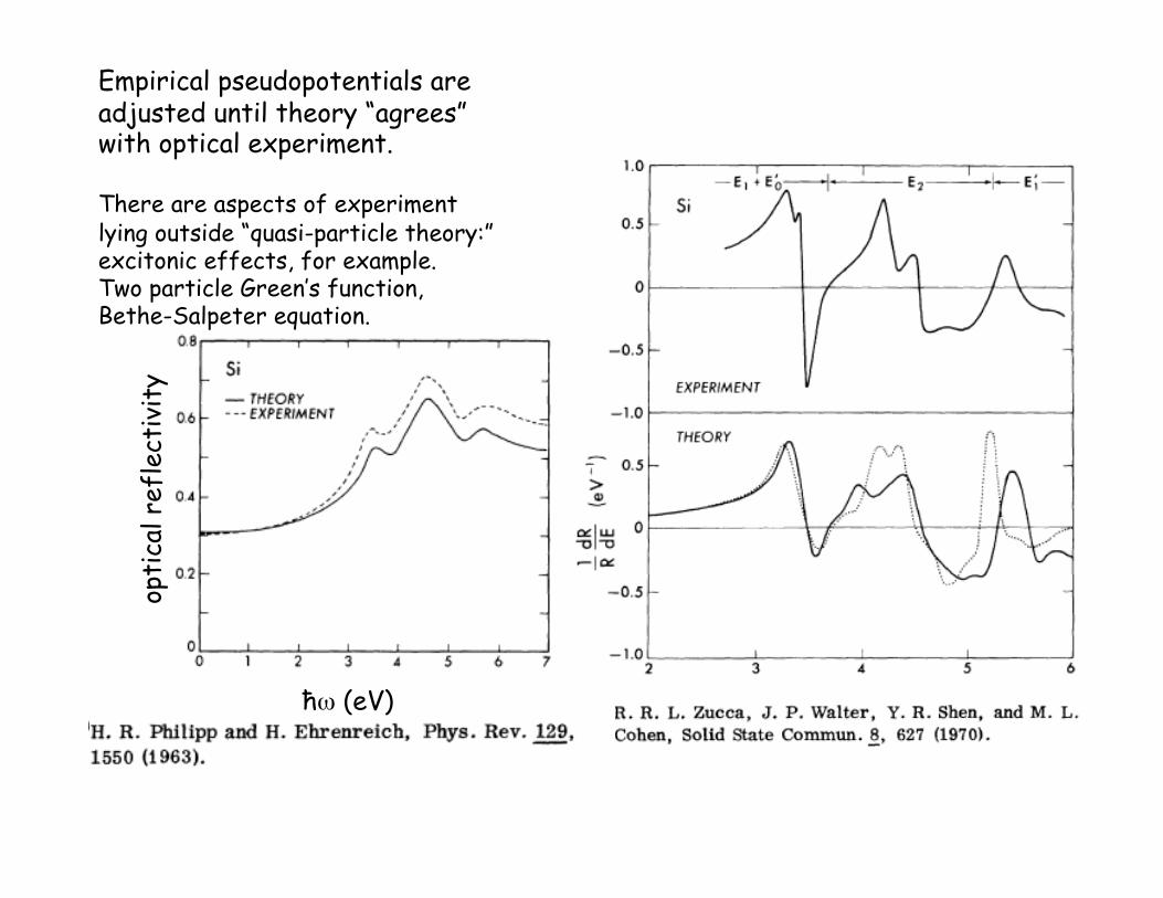
Empirical pseudopotentials are adjusted until theory “agrees” with optical experiment.

There are aspects of experiment lying outside “quasi-particle theory:” excitonic effects, for example. Two particle Green’s function, Bethe-Salpeter equation.

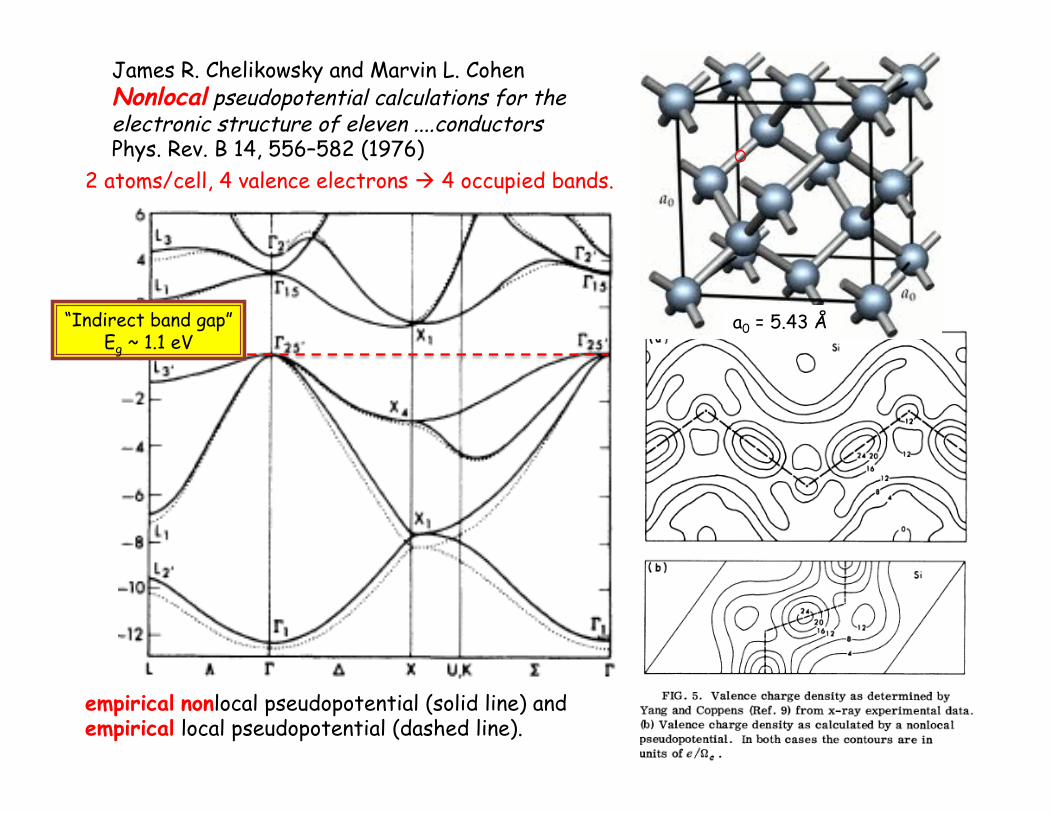
James R. Chelikowsky and Marvin L. Cohen Nonlocal pseudopotential calculations for the electronic structure of eleven ....conductors Phys. Rev. B 14, 556–582 (1976)

empirical nonlocal pseudopotential (solid line) and empirical local pseudopotential (dashed line).

a0 = 5.43 Å

2 atoms/cell, 4 valence electrons ! 4 occupied bands.

“Indirect band gap” Eg ~ 1.1 eV

Elec

tron

ic d

ensi

ty o

f st

ates

predicted electron quasiparticle energy

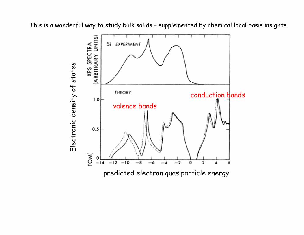
valence bands conduction bands

This is a wonderful way to study bulk solids – supplemented by chemical local basis insights.

Around 1980, self-consistent calculations had become attainable. “Ab initio” (i.e. non-empirical, no adjusting) had become desirable.

Why? It worsened quasiparticle properties. The “band-gap problem” emerged with ab initio theory.

Answer: surface physics!

DFT promises ground state properties, especially total energy – These had not been the target of previous semi-empirical approaches.

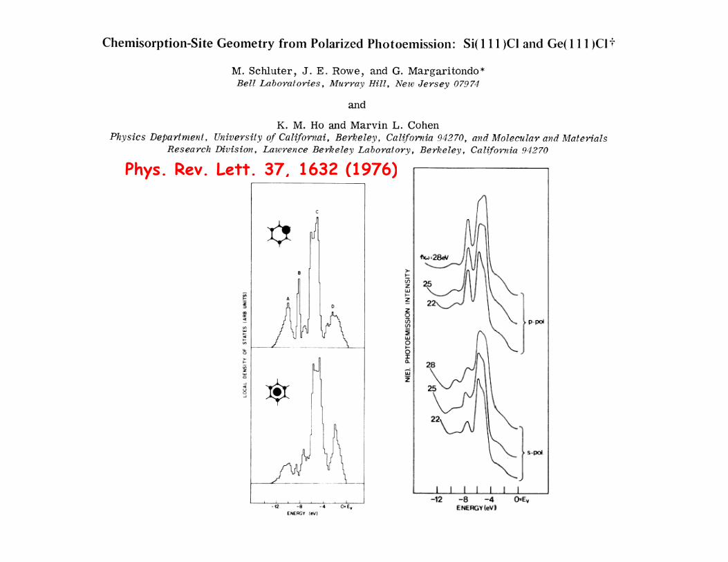
Phys. Rev. Lett. 37, 1632 (1976)

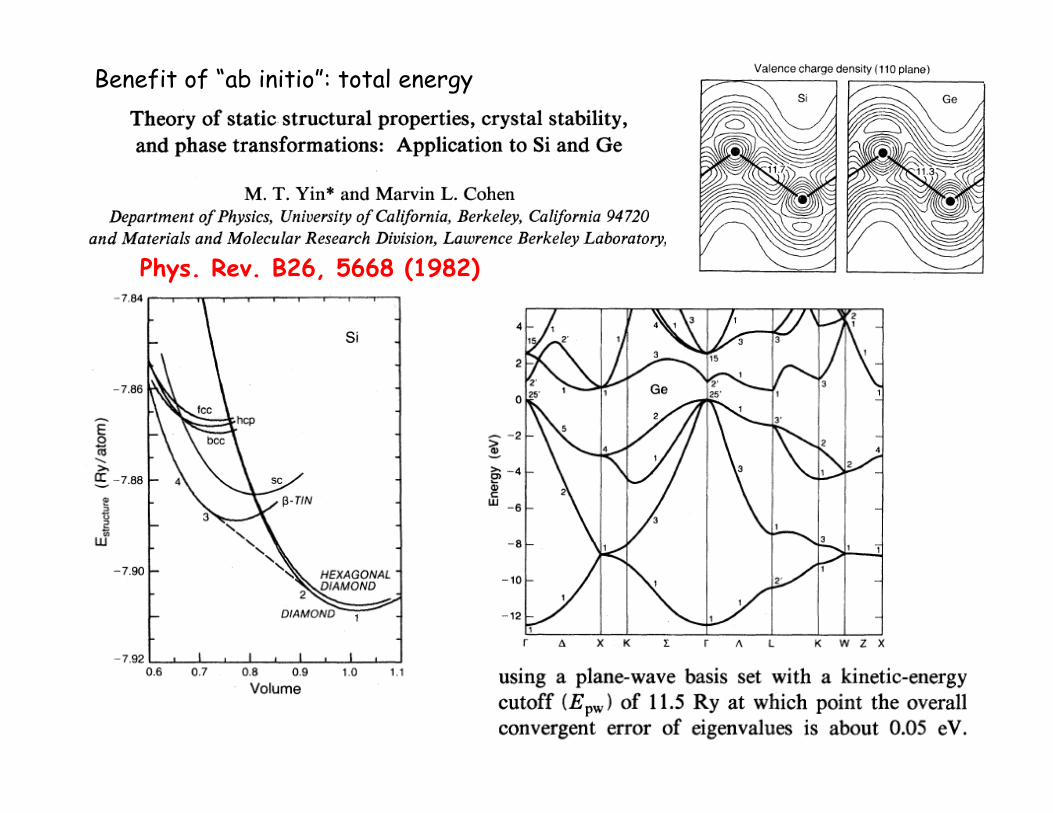
Phys. Rev. B26, 5668 (1982)

Benefit of “ab initio”: total energy

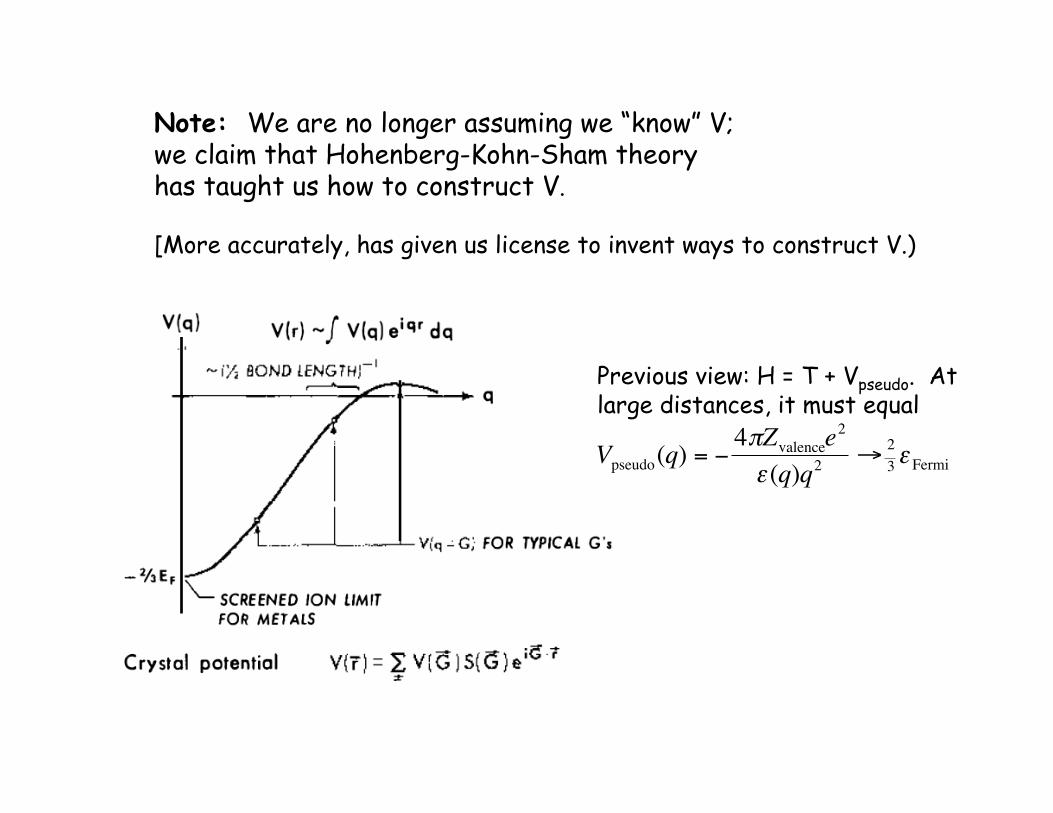
Note: We are no longer assuming we “know” V; we claim that Hohenberg-Kohn-Sham theory has taught us how to construct V.

[More accurately, has given us license to invent ways to construct V.)

Previous view: H = T + Vpseudo. At large distances, it must equal

€

Vpseudo(q) = −4πZvalencee

2

ε (q)q2→ 2

3ε Fermi

€

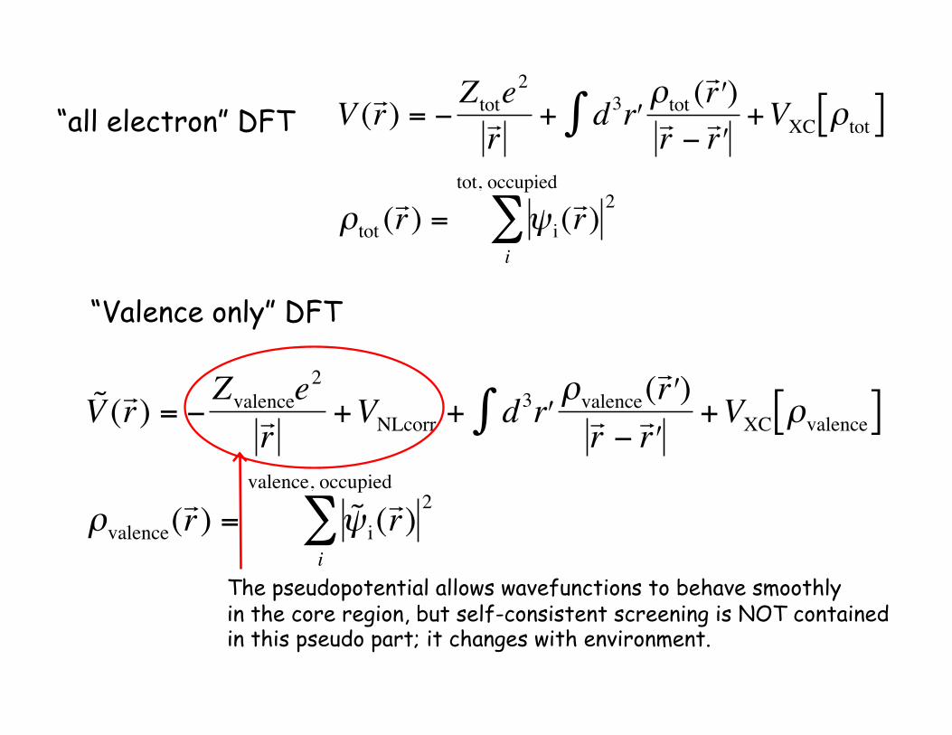
V (! r ) = −Ztote

2

! r + d3 ʹ′ r ∫ ρtot (

! ʹ′ r )

! r − ! ʹ′ r +VXC ρtot[ ]

ρtot (! r ) = ψ i (

! r ) 2

i

tot, occupied

∑

€

˜ V (! r ) = −Zvalencee

2

! r +VNLcorr + d3 ʹ′ r ∫ ρvalence(

! ʹ′ r )

! r − ! ʹ′ r +VXC ρvalence[ ]

ρvalence(! r ) = ˜ ψ i (

! r ) 2

i

valence, occupied

∑

“all electron” DFT

“Valence only” DFT

The pseudopotential allows wavefunctions to behave smoothly in the core region, but self-consistent screening is NOT contained in this pseudo part; it changes with environment.

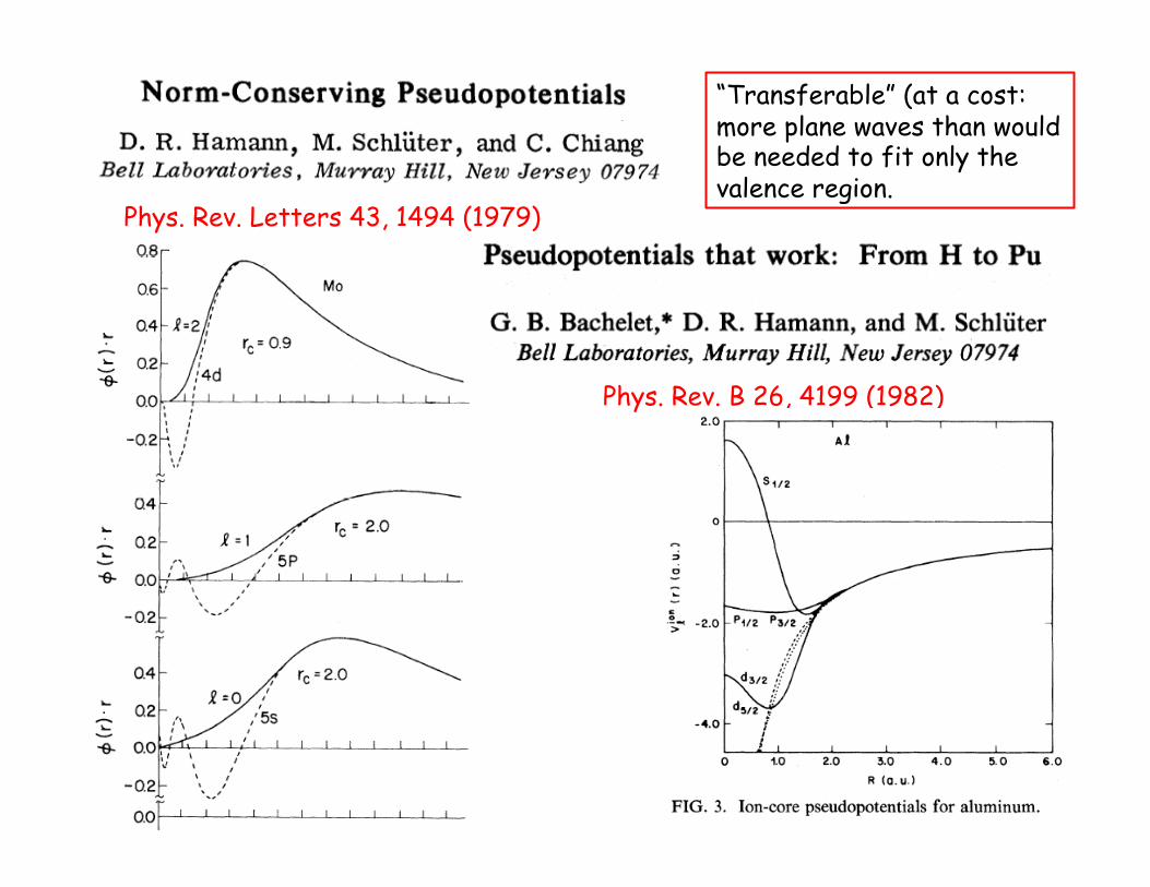
Phys. Rev. Letters 43, 1494 (1979)

Phys. Rev. B 26, 4199 (1982)

“Transferable” (at a cost: more plane waves than would be needed to fit only the valence region.

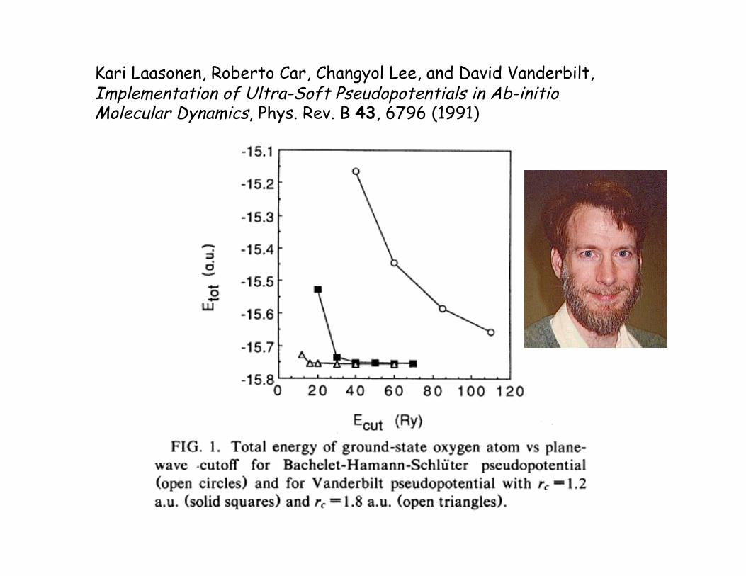
Kari Laasonen, Roberto Car, Changyol Lee, and David Vanderbilt, Implementation of Ultra-Soft Pseudopotentials in Ab-initio Molecular Dynamics, Phys. Rev. B 43, 6796 (1991)

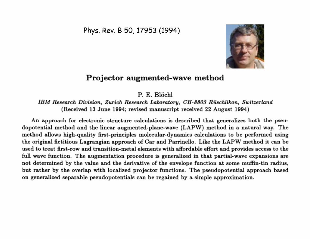
Phys. Rev. B 50, 17953 (1994)

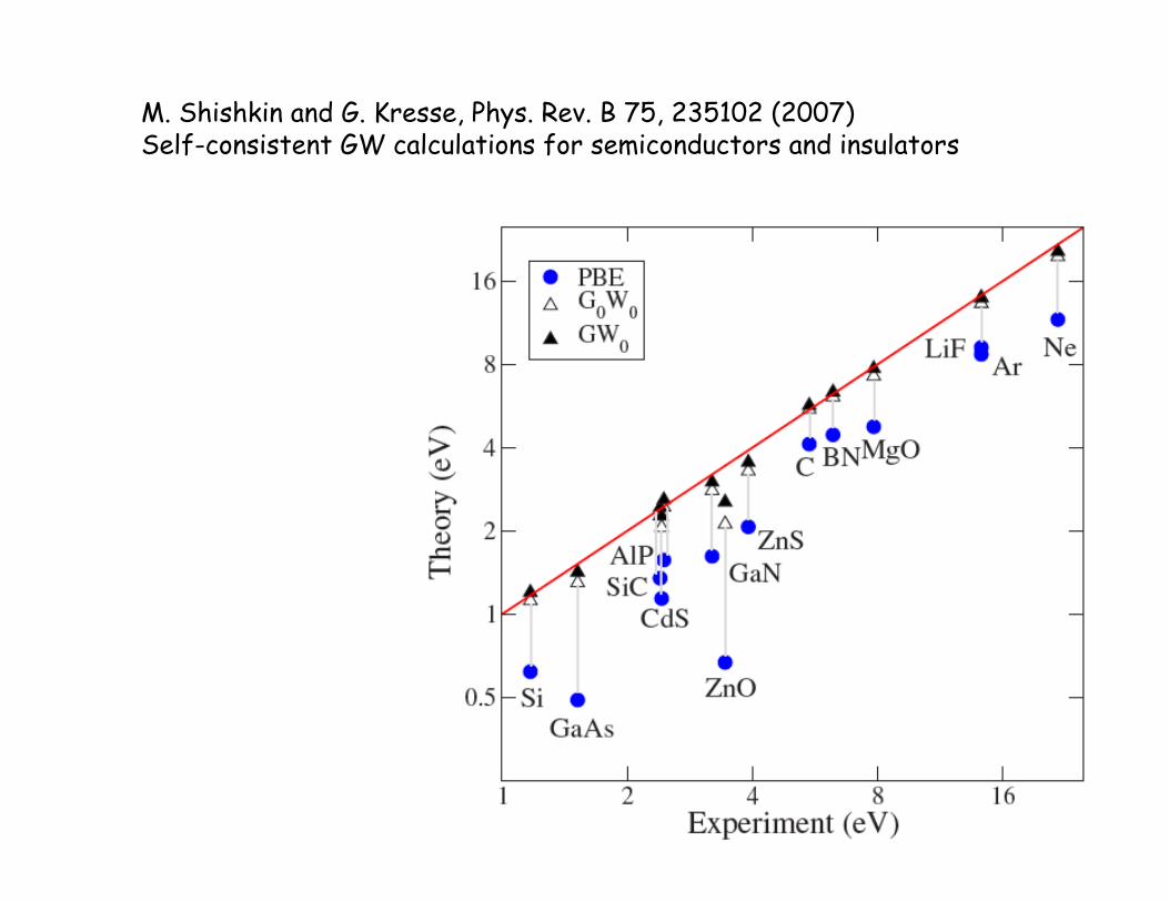
M. Shishkin and G. Kresse, Phys. Rev. B 75, 235102 (2007) Self-consistent GW calculations for semiconductors and insulators

Thank you to all my electronic structure collaborators, especially

Marvin Cohen Warren Pickett Bill Butler Jim Davenport Mike Weinert Renata Wentzcovitch Mark Hybertsen Jim Muckerman Marivi Fernandez-Serra Artem Oganov

and Manuel Cardona, who watched me do one by myself.