Introduction to Mathematical Fluid Dynamics-IIIruediger/pages/vortraege/ws1011/mengxu/... ·...
49
Introduction to Mathematical Fluid Dynamics-III The Navier-Stokes Equations Meng Xu Department of Mathematics University of Wyoming Bergische Universität Wuppertal Math Fluid Dynamics-III
Transcript of Introduction to Mathematical Fluid Dynamics-IIIruediger/pages/vortraege/ws1011/mengxu/... ·...
Introduction to Mathematical Fluid Dynamics-IIIThe Navier-Stokes Equations
Meng Xu
Department of MathematicsUniversity of Wyoming
Bergische Universität Wuppertal Math Fluid Dynamics-III
Euler equations
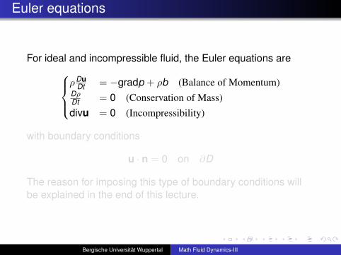
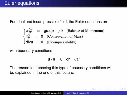
For ideal and incompressible fluid, the Euler equations areρDu
Dt = −gradp + ρb (Balance of Momentum)DρDt = 0 (Conservation of Mass)divu = 0 (Incompressibility)
with boundary conditions
u · n = 0 on ∂D
The reason for imposing this type of boundary conditions willbe explained in the end of this lecture.
Bergische Universität Wuppertal Math Fluid Dynamics-III
Euler equations
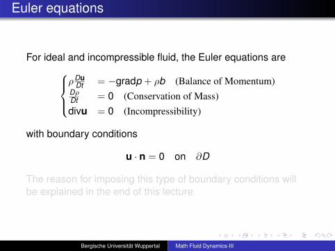
For ideal and incompressible fluid, the Euler equations areρDu
Dt = −gradp + ρb (Balance of Momentum)DρDt = 0 (Conservation of Mass)divu = 0 (Incompressibility)
with boundary conditions
u · n = 0 on ∂D
The reason for imposing this type of boundary conditions willbe explained in the end of this lecture.
Bergische Universität Wuppertal Math Fluid Dynamics-III
Balance of momentum
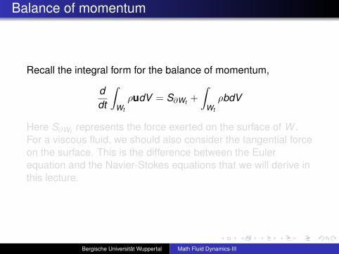
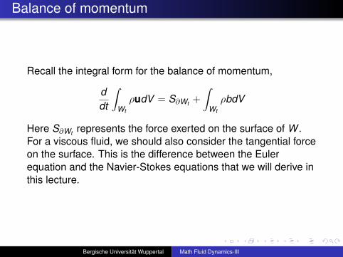
Recall the integral form for the balance of momentum,
ddt
∫Wt
ρudV = S∂Wt +
∫Wt
ρbdV
Here S∂Wt represents the force exerted on the surface of W .For a viscous fluid, we should also consider the tangential forceon the surface. This is the difference between the Eulerequation and the Navier-Stokes equations that we will derive inthis lecture.
Bergische Universität Wuppertal Math Fluid Dynamics-III
Balance of momentum
Recall the integral form for the balance of momentum,
ddt
∫Wt
ρudV = S∂Wt +
∫Wt
ρbdV
Here S∂Wt represents the force exerted on the surface of W .For a viscous fluid, we should also consider the tangential forceon the surface. This is the difference between the Eulerequation and the Navier-Stokes equations that we will derive inthis lecture.
Bergische Universität Wuppertal Math Fluid Dynamics-III
Stress tensor
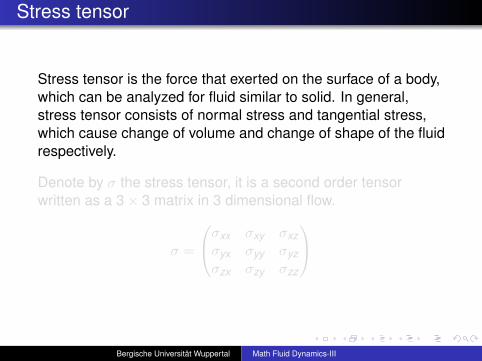
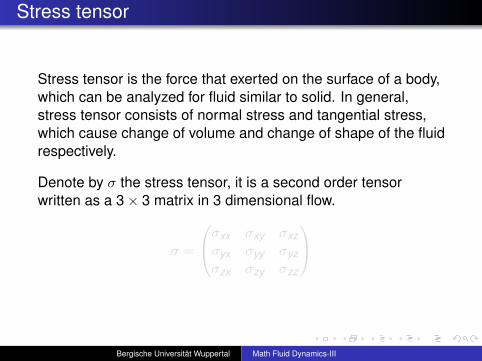
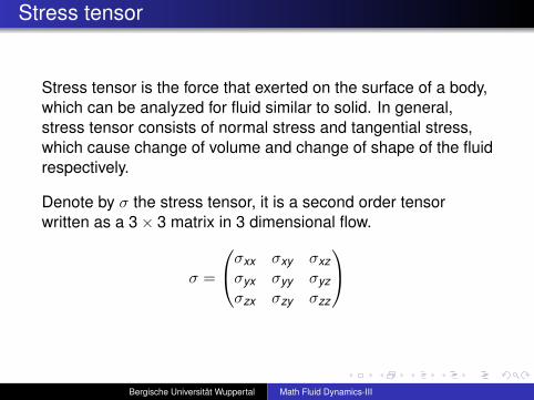
Stress tensor is the force that exerted on the surface of a body,which can be analyzed for fluid similar to solid. In general,stress tensor consists of normal stress and tangential stress,which cause change of volume and change of shape of the fluidrespectively.
Denote by σ the stress tensor, it is a second order tensorwritten as a 3× 3 matrix in 3 dimensional flow.
σ =
σxx σxy σxzσyx σyy σyzσzx σzy σzz
Bergische Universität Wuppertal Math Fluid Dynamics-III
Stress tensor
Stress tensor is the force that exerted on the surface of a body,which can be analyzed for fluid similar to solid. In general,stress tensor consists of normal stress and tangential stress,which cause change of volume and change of shape of the fluidrespectively.
Denote by σ the stress tensor, it is a second order tensorwritten as a 3× 3 matrix in 3 dimensional flow.
σ =
σxx σxy σxzσyx σyy σyzσzx σzy σzz
Bergische Universität Wuppertal Math Fluid Dynamics-III
Normal stress tensor
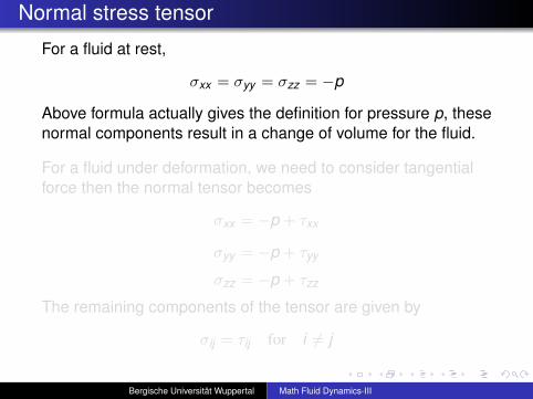
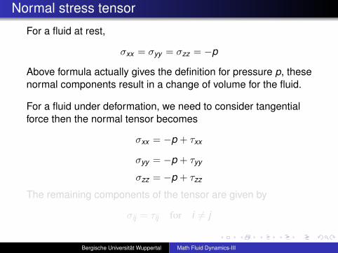
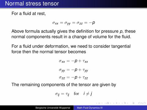
For a fluid at rest,
σxx = σyy = σzz = −p
Above formula actually gives the definition for pressure p, thesenormal components result in a change of volume for the fluid.
For a fluid under deformation, we need to consider tangentialforce then the normal tensor becomes
σxx = −p + τxx
σyy = −p + τyy
σzz = −p + τzz
The remaining components of the tensor are given by
σij = τij for i 6= j
Bergische Universität Wuppertal Math Fluid Dynamics-III

Normal stress tensor
For a fluid at rest,
σxx = σyy = σzz = −p
Above formula actually gives the definition for pressure p, thesenormal components result in a change of volume for the fluid.
For a fluid under deformation, we need to consider tangentialforce then the normal tensor becomes
σxx = −p + τxx
σyy = −p + τyy
σzz = −p + τzz
The remaining components of the tensor are given by
σij = τij for i 6= j
Bergische Universität Wuppertal Math Fluid Dynamics-III
Deviatoric tensor
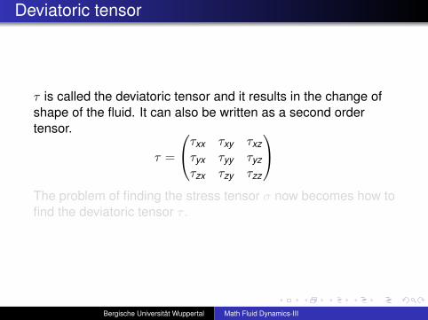
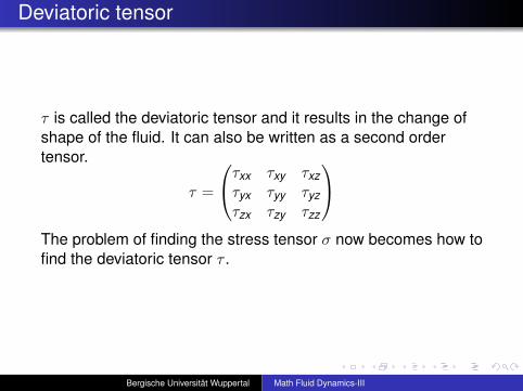
τ is called the deviatoric tensor and it results in the change ofshape of the fluid. It can also be written as a second ordertensor.
τ =
τxx τxy τxzτyx τyy τyzτzx τzy τzz
The problem of finding the stress tensor σ now becomes how tofind the deviatoric tensor τ .
Bergische Universität Wuppertal Math Fluid Dynamics-III
Deviatoric tensor
τ is called the deviatoric tensor and it results in the change ofshape of the fluid. It can also be written as a second ordertensor.
τ =
τxx τxy τxzτyx τyy τyzτzx τzy τzz
The problem of finding the stress tensor σ now becomes how tofind the deviatoric tensor τ .
Bergische Universität Wuppertal Math Fluid Dynamics-III
Strain tensor
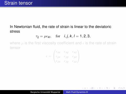
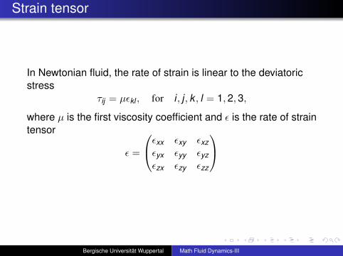
In Newtonian fluid, the rate of strain is linear to the deviatoricstress
τij = µεkl , for i , j , k , l = 1,2,3,
where µ is the first viscosity coefficient and ε is the rate of straintensor
ε =
εxx εxy εxzεyx εyy εyzεzx εzy εzz
Bergische Universität Wuppertal Math Fluid Dynamics-III
Strain tensor
In Newtonian fluid, the rate of strain is linear to the deviatoricstress
τij = µεkl , for i , j , k , l = 1,2,3,
where µ is the first viscosity coefficient and ε is the rate of straintensor
ε =
εxx εxy εxzεyx εyy εyzεzx εzy εzz
Bergische Universität Wuppertal Math Fluid Dynamics-III
Strain tensor
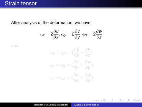
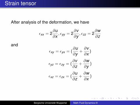
After analysis of the deformation, we have
εxx = 2∂u∂x, εyy = 2
∂v∂y, εzz = 2
∂w∂z
andεxy = εyx = (
∂u∂y
+∂v∂x
)
εyz = εzy = (∂v∂z
+∂w∂y
)
εxz = εzx = (∂u∂z
+∂w∂x
)
Bergische Universität Wuppertal Math Fluid Dynamics-III
Strain tensor
After analysis of the deformation, we have
εxx = 2∂u∂x, εyy = 2
∂v∂y, εzz = 2
∂w∂z
andεxy = εyx = (
∂u∂y
+∂v∂x
)
εyz = εzy = (∂v∂z
+∂w∂y
)
εxz = εzx = (∂u∂z
+∂w∂x
)
Bergische Universität Wuppertal Math Fluid Dynamics-III
Normal direction
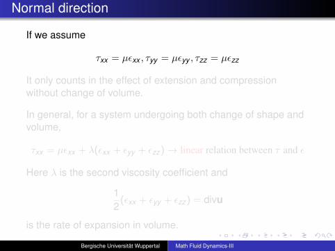
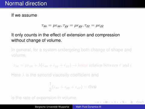
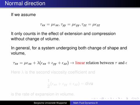
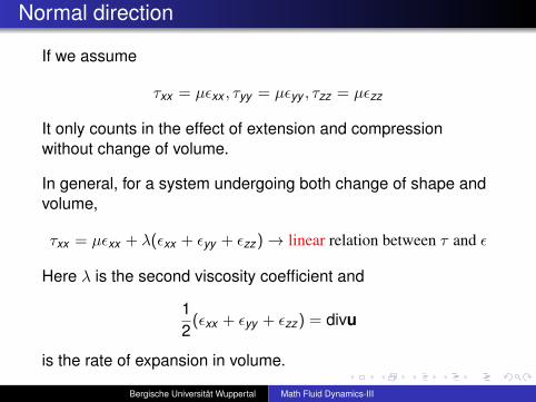
If we assume
τxx = µεxx , τyy = µεyy , τzz = µεzz
It only counts in the effect of extension and compressionwithout change of volume.
In general, for a system undergoing both change of shape andvolume,
τxx = µεxx + λ(εxx + εyy + εzz)→ linear relation between τ and ε
Here λ is the second viscosity coefficient and
12(εxx + εyy + εzz) = divu
is the rate of expansion in volume.
Bergische Universität Wuppertal Math Fluid Dynamics-III
Normal direction
If we assume
τxx = µεxx , τyy = µεyy , τzz = µεzz
It only counts in the effect of extension and compressionwithout change of volume.
In general, for a system undergoing both change of shape andvolume,
τxx = µεxx + λ(εxx + εyy + εzz)→ linear relation between τ and ε
Here λ is the second viscosity coefficient and
12(εxx + εyy + εzz) = divu
is the rate of expansion in volume.
Bergische Universität Wuppertal Math Fluid Dynamics-III
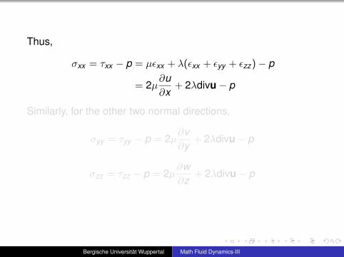
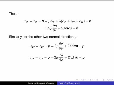
Thus,
σxx = τxx − p = µεxx + λ(εxx + εyy + εzz)− p
= 2µ∂u∂x
+ 2λdivu− p
Similarly, for the other two normal directions,
σyy = τyy − p = 2µ∂v∂y
+ 2λdivu− p
σzz = τzz − p = 2µ∂w∂z
+ 2λdivu− p
Bergische Universität Wuppertal Math Fluid Dynamics-III
Thus,
σxx = τxx − p = µεxx + λ(εxx + εyy + εzz)− p
= 2µ∂u∂x
+ 2λdivu− p
Similarly, for the other two normal directions,
σyy = τyy − p = 2µ∂v∂y
+ 2λdivu− p
σzz = τzz − p = 2µ∂w∂z
+ 2λdivu− p
Bergische Universität Wuppertal Math Fluid Dynamics-III
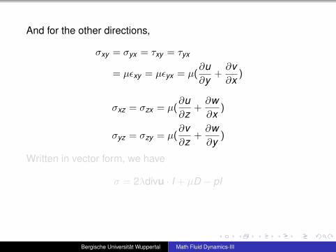
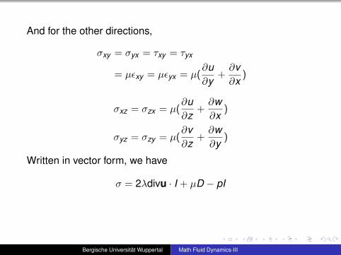
And for the other directions,
σxy = σyx = τxy = τyx
= µεxy = µεyx = µ(∂u∂y
+∂v∂x
)
σxz = σzx = µ(∂u∂z
+∂w∂x
)
σyz = σzy = µ(∂v∂z
+∂w∂y
)
Written in vector form, we have
σ = 2λdivu · I + µD − pI
Bergische Universität Wuppertal Math Fluid Dynamics-III
And for the other directions,
σxy = σyx = τxy = τyx
= µεxy = µεyx = µ(∂u∂y
+∂v∂x
)
σxz = σzx = µ(∂u∂z
+∂w∂x
)
σyz = σzy = µ(∂v∂z
+∂w∂y
)
Written in vector form, we have
σ = 2λdivu · I + µD − pI
Bergische Universität Wuppertal Math Fluid Dynamics-III
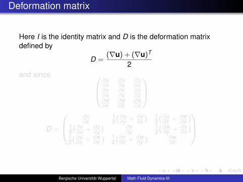
Deformation matrix
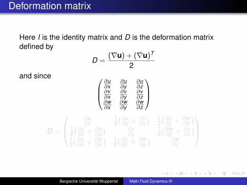
Here I is the identity matrix and D is the deformation matrixdefined by
D =(∇u) + (∇u)T
2and since
∂u∂x
∂u∂y
∂u∂z
∂v∂x
∂v∂y
∂v∂z
∂w∂x
∂w∂y
∂w∂z
D =
∂u∂x
12(∂u∂y + ∂v
∂x )12(∂u∂z + ∂w
∂x )12(∂v∂x + ∂u
∂y )∂v∂y
12(∂w∂y + ∂v
∂z )12(∂u∂z + ∂w
∂x )12(∂v∂z + ∂w
∂y )∂w∂z
Bergische Universität Wuppertal Math Fluid Dynamics-III
Deformation matrix
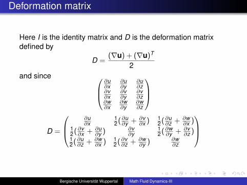
Here I is the identity matrix and D is the deformation matrixdefined by
D =(∇u) + (∇u)T
2and since
∂u∂x
∂u∂y
∂u∂z
∂v∂x
∂v∂y
∂v∂z
∂w∂x
∂w∂y
∂w∂z
D =
∂u∂x
12(∂u∂y + ∂v
∂x )12(∂u∂z + ∂w
∂x )12(∂v∂x + ∂u
∂y )∂v∂y
12(∂w∂y + ∂v
∂z )12(∂u∂z + ∂w
∂x )12(∂v∂z + ∂w
∂y )∂w∂z
Bergische Universität Wuppertal Math Fluid Dynamics-III
Deformation matrix
Here I is the identity matrix and D is the deformation matrixdefined by
D =(∇u) + (∇u)T
2and since
∂u∂x
∂u∂y
∂u∂z
∂v∂x
∂v∂y
∂v∂z
∂w∂x
∂w∂y
∂w∂z
D =
∂u∂x
12(∂u∂y + ∂v
∂x )12(∂u∂z + ∂w
∂x )12(∂v∂x + ∂u
∂y )∂v∂y
12(∂w∂y + ∂v
∂z )12(∂u∂z + ∂w
∂x )12(∂v∂z + ∂w
∂y )∂w∂z
Bergische Universität Wuppertal Math Fluid Dynamics-III
Force on the surface
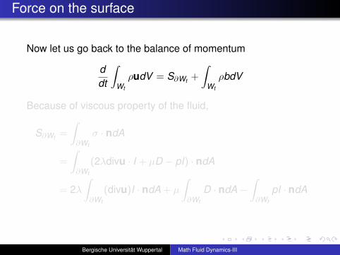
Now let us go back to the balance of momentum
ddt
∫Wt
ρudV = S∂Wt +
∫Wt
ρbdV
Because of viscous property of the fluid,
S∂Wt =
∫∂Wt
σ · ndA
=
∫∂Wt
(2λdivu · I + µD − pI) · ndA
= 2λ∫∂Wt
(divu)I · ndA + µ
∫∂Wt
D · ndA−∫∂Wt
pI · ndA
Bergische Universität Wuppertal Math Fluid Dynamics-III
Force on the surface
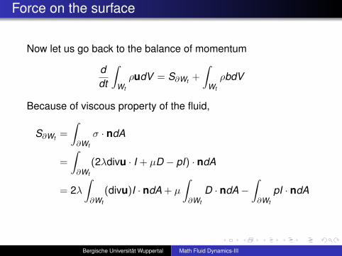
Now let us go back to the balance of momentum
ddt
∫Wt
ρudV = S∂Wt +
∫Wt
ρbdV
Because of viscous property of the fluid,
S∂Wt =
∫∂Wt
σ · ndA
=
∫∂Wt
(2λdivu · I + µD − pI) · ndA
= 2λ∫∂Wt
(divu)I · ndA + µ
∫∂Wt
D · ndA−∫∂Wt
pI · ndA
Bergische Universität Wuppertal Math Fluid Dynamics-III
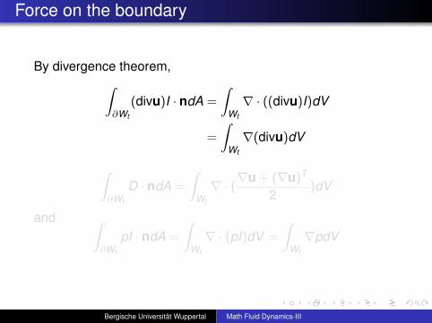
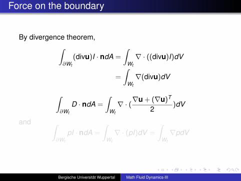
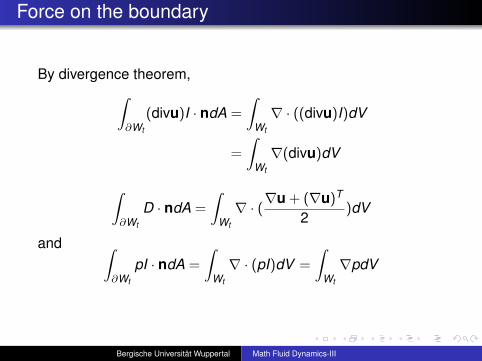
Force on the boundary
By divergence theorem,∫∂Wt
(divu)I · ndA =
∫Wt
∇ · ((divu)I)dV
=
∫Wt
∇(divu)dV
∫∂Wt
D · ndA =
∫Wt
∇ · (∇u + (∇u)T
2)dV
and ∫∂Wt
pI · ndA =
∫Wt
∇ · (pI)dV =
∫Wt
∇pdV
Bergische Universität Wuppertal Math Fluid Dynamics-III
Force on the boundary
By divergence theorem,∫∂Wt
(divu)I · ndA =
∫Wt
∇ · ((divu)I)dV
=
∫Wt
∇(divu)dV
∫∂Wt
D · ndA =
∫Wt
∇ · (∇u + (∇u)T
2)dV
and ∫∂Wt
pI · ndA =
∫Wt
∇ · (pI)dV =
∫Wt
∇pdV
Bergische Universität Wuppertal Math Fluid Dynamics-III
Force on the boundary
By divergence theorem,∫∂Wt
(divu)I · ndA =
∫Wt
∇ · ((divu)I)dV
=
∫Wt
∇(divu)dV
∫∂Wt
D · ndA =
∫Wt
∇ · (∇u + (∇u)T
2)dV
and ∫∂Wt
pI · ndA =
∫Wt
∇ · (pI)dV =
∫Wt
∇pdV
Bergische Universität Wuppertal Math Fluid Dynamics-III
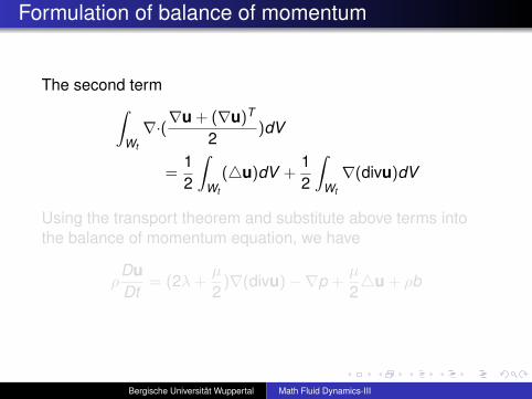
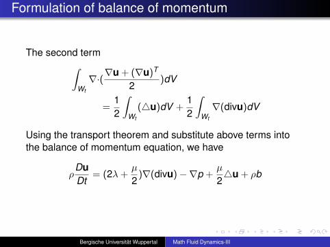
Formulation of balance of momentum
The second term∫Wt
∇·(∇u + (∇u)T
2)dV
=12
∫Wt
(4u)dV +12
∫Wt
∇(divu)dV
Using the transport theorem and substitute above terms intothe balance of momentum equation, we have
ρDuDt
= (2λ+µ
2)∇(divu)−∇p +
µ
24u + ρb
Bergische Universität Wuppertal Math Fluid Dynamics-III
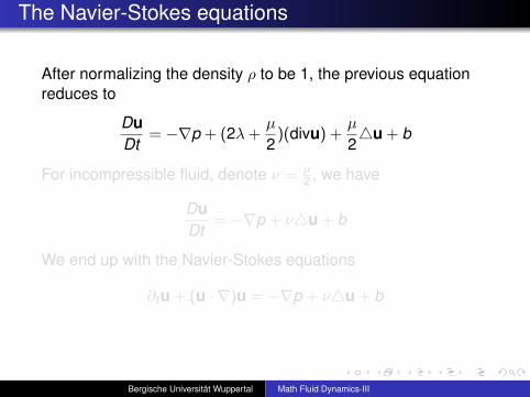
The Navier-Stokes equations
After normalizing the density ρ to be 1, the previous equationreduces to
DuDt
= −∇p + (2λ+µ
2)(divu) +
µ
24u + b
For incompressible fluid, denote ν = µ2 , we have
DuDt
= −∇p + ν4u + b
We end up with the Navier-Stokes equations
∂tu + (u · ∇)u = −∇p + ν4u + b
Bergische Universität Wuppertal Math Fluid Dynamics-III
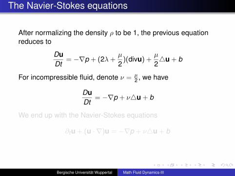
The Navier-Stokes equations
After normalizing the density ρ to be 1, the previous equationreduces to
DuDt
= −∇p + (2λ+µ
2)(divu) +
µ
24u + b
For incompressible fluid, denote ν = µ2 , we have
DuDt
= −∇p + ν4u + b
We end up with the Navier-Stokes equations
∂tu + (u · ∇)u = −∇p + ν4u + b
Bergische Universität Wuppertal Math Fluid Dynamics-III
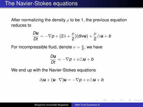
The Navier-Stokes equations
After normalizing the density ρ to be 1, the previous equationreduces to
DuDt
= −∇p + (2λ+µ
2)(divu) +
µ
24u + b
For incompressible fluid, denote ν = µ2 , we have
DuDt
= −∇p + ν4u + b
We end up with the Navier-Stokes equations
∂tu + (u · ∇)u = −∇p + ν4u + b
Bergische Universität Wuppertal Math Fluid Dynamics-III
Boundary conditions for Euler and N-S equations
We end this lecture with a discussion on the boundaryconditions we should impose for the Euler and Navier-Stokesequations.
For Euler’s equations for ideal flow we use u · n = 0, that is,fluid does not cross the boundary but may move tangentially tothe boundary.
For the Navier-Stokes equations, the extra term ν4u raises thenumber of derivatives of u. For both experimental andmathematical reasons, this is accompanied by an increase inthe number of boundary conditions.
Bergische Universität Wuppertal Math Fluid Dynamics-III
Mathematical reason
For instance, on a solid wall at rest we add the condition thatthe tangential velocity also be zero ("no-slip condition"), so thefull boundary condition are simply
u = 0 on solid walls at rest
The mathematical need for extra boundary conditions lies ontheir role in proving that the equations are well posed, that is, aunique solution exists and depends continuously on the initialdata.
Bergische Universität Wuppertal Math Fluid Dynamics-III
Physical reason
The physical need for the extra boundary conditions comesfrom simple experiments involving flow past a solid wall. Forexample, if dye is injected into flow down a pipe and is carefullywatched near the boundary, one sees that the velocityapproaches zero at the boundary to a high degree of precision.
The no-slip condition is also reasonable if one contemplates thephysical mechanism responsible for the viscous terms, namely,molecular diffusion. Our example indicates that molecularinteraction between the solid wall with zero tangential velocityshould impart the same condition to the immediately adjacentfluid.
Bergische Universität Wuppertal Math Fluid Dynamics-III
Final remark
Another crucial feature of the boundary condition u = 0 is that itprovides a mechanism by which a boundary can producevorticity in the fluid. But we will not talk about rotation andvorticity of fluid in this lecture.
Bergische Universität Wuppertal Math Fluid Dynamics-III