
Introduction to Linear Mixed-E ect Models
46
Introduction to Linear Mixed-Effect Models Niels Hagenbuch March 1, 2010
Transcript of Introduction to Linear Mixed-E ect Models

Introduction to Linear Mixed-Effect Models
Niels Hagenbuch
March 1, 2010
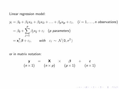
Linear regression model:
yi = β0 + β1xi1 + β2xi2 + . . .+ βpxip + εi , (i = 1, . . . , n observations)
= β0 +
p∑j=1
βjxij + εi (p parameters)
= xTi β + εi , with εi ∼ N〈 0, σ2 〉
or in matrix notation:
y = X × β + ε(n × 1) (n × p) (p × 1) (n × 1)
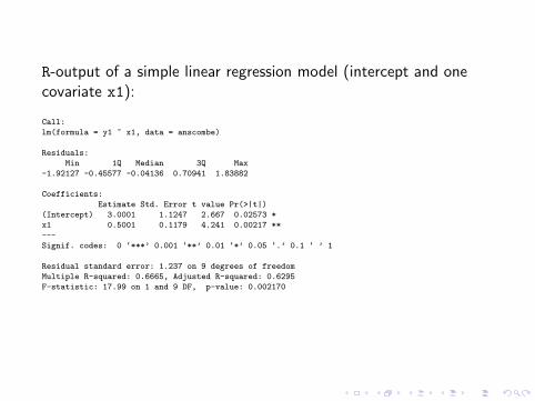
R-output of a simple linear regression model (intercept and onecovariate x1):
Call:
lm(formula = y1 ~ x1, data = anscombe)
Residuals:
Min 1Q Median 3Q Max
-1.92127 -0.45577 -0.04136 0.70941 1.83882
Coefficients:
Estimate Std. Error t value Pr(>|t|)
(Intercept) 3.0001 1.1247 2.667 0.02573 *
x1 0.5001 0.1179 4.241 0.00217 **
---
Signif. codes: 0 ‘***’ 0.001 ‘**’ 0.01 ‘*’ 0.05 ‘.’ 0.1 ‘ ’ 1
Residual standard error: 1.237 on 9 degrees of freedom
Multiple R-squared: 0.6665, Adjusted R-squared: 0.6295
F-statistic: 17.99 on 1 and 9 DF, p-value: 0.002170
●
●
●
●
●
●
●
●
●
●
●
0 5 10 15 20
05
1015
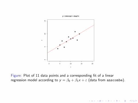
y = intercept + slope*x
x
y
Figure: Plot of 11 data points and a corresponding fit of a linearregression model according to y = β0 + β1x + ε (data from anscombe).
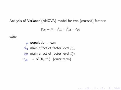
Analysis of Variance (ANOVA) model for two (crossed) factors:
yijk = µ+ βi1 + βj2 + εijk
with:
µ population mean
βi1 main effect of factor level βi1
βj2 main effect of factor level βj2
εijk ∼ N〈 0, σ2 〉 (error term)
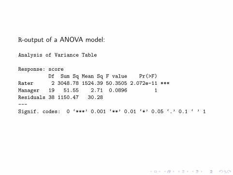
R-output of a ANOVA model:
Analysis of Variance Table
Response: score
Df Sum Sq Mean Sq F value Pr(>F)
Rater 2 3048.78 1524.39 50.3505 2.072e-11 ***
Manager 19 51.55 2.71 0.0896 1
Residuals 38 1150.47 30.28
---
Signif. codes: 0 ‘***’ 0.001 ‘**’ 0.01 ‘*’ 0.05 ‘.’ 0.1 ‘ ’ 1

Classical Analysis of Variance (ANOVA)
I Classical ANOVA developed for agricultural experimentsI Control over
I crop varietiesI type of fertilizers usedI amount of fertilizerI plots, subplotsI greenhouse: light, irrigation, soil type, etc.
I Need for randomization in order to avoid confounding
I Different designs
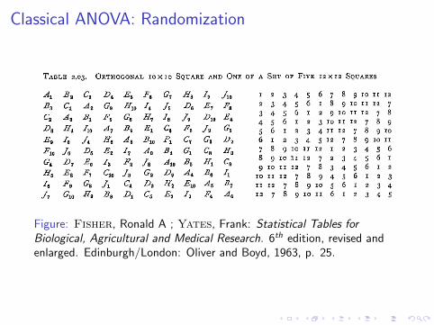
Classical ANOVA: Randomization
Figure: Fisher, Ronald A ; Yates, Frank: Statistical Tables forBiological, Agricultural and Medical Research. 6th edition, revised andenlarged. Edinburgh/London: Oliver and Boyd, 1963, p. 25.
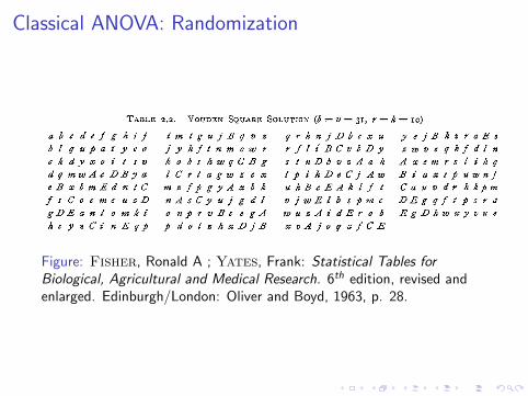
Classical ANOVA: Randomization
Figure: Fisher, Ronald A ; Yates, Frank: Statistical Tables forBiological, Agricultural and Medical Research. 6th edition, revised andenlarged. Edinburgh/London: Oliver and Boyd, 1963, p. 28.

Experimental Design: Crossed vs. Nested
I Two factors are said to be crossed if all levels of the first factorappear in combination with all levels of the other factor.
I A crossed design is also called factorial.
I Example: five enzymes are tested in two solutions with different pH(four measurements each).
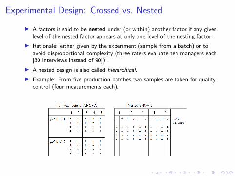
Experimental Design: Crossed vs. Nested
I A factors is said to be nested under (or within) another factor if any givenlevel of the nested factor appears at only one level of the nesting factor.
I Rationale: either given by the experiment (sample from a batch) or toavoid disproportional complexity (three raters evaluate ten managers each[30 interviews instead of 90]).
I A nested design is also called hierarchical.
I Example: From five production batches two samples are taken for qualitycontrol (four measurements each).
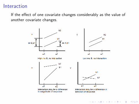
Interaction
If the effect of one covariate changes considerably as the value ofanother covariate changes.
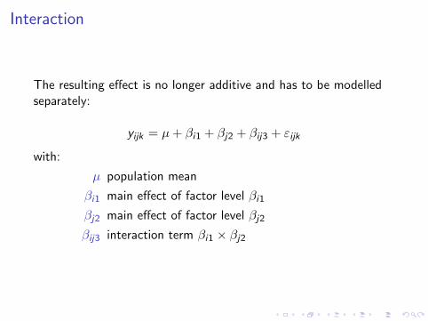
Interaction
The resulting effect is no longer additive and has to be modelledseparately:
yijk = µ+ βi1 + βj2 + βij3 + εijk
with:
µ population mean
βi1 main effect of factor level βi1
βj2 main effect of factor level βj2
βij3 interaction term βi1 × βj2

Fixed vs. Random Effects
I So far, covariates were considered fixed.
I Levels were chosen deliberately
I Levels had a specific meaning
I Changing levels leads to fundamental changes in theexperiment
Examples:
1. Different crop varieties (oat; oat and rye; oat, rye, barley)
2. Medical test on humans (males; males and females)
3. Life expectancy (german speaking countries; german and french; german,french, italian)
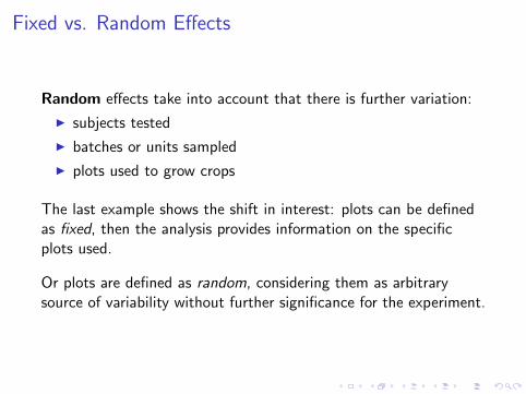
Fixed vs. Random Effects
Random effects take into account that there is further variation:
I subjects tested
I batches or units sampled
I plots used to grow crops
The last example shows the shift in interest: plots can be definedas fixed, then the analysis provides information on the specificplots used.
Or plots are defined as random, considering them as arbitrarysource of variability without further significance for the experiment.

Random Effects
Random effects
I assess variability
I reduce threats to validity
I increase generalizability
Random effects allow to generalize
I the results: schools in Markus’ nano-introduction
I the research question: can a research method be used“universally”?
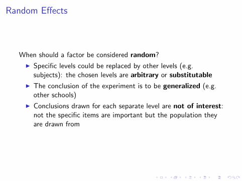
Random Effects
When should a factor be considered random?
I Specific levels could be replaced by other levels (e.g.subjects): the chosen levels are arbitrary or substitutable
I The conclusion of the experiment is to be generalized (e.g.other schools)
I Conclusions drawn for each separate level are not of interest:not the specific items are important but the population theyare drawn from
Model
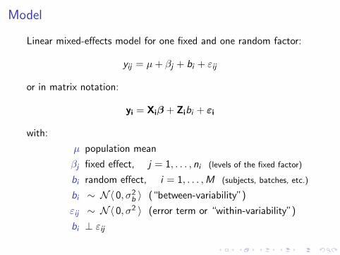
Linear mixed-effects model for one fixed and one random factor:
yij = µ+ βj + bi + εij
or in matrix notation:
yi = Xiβ + Zibi + εi
with:
µ population mean
βj fixed effect, j = 1, . . . , ni (levels of the fixed factor)
bi random effect, i = 1, . . . ,M (subjects, batches, etc.)
bi ∼ N〈 0, σ2b 〉 (“between-variability”)
εij ∼ N〈 0, σ2 〉 (error term or “within-variability”)
bi ⊥ εij
Software
The new variance term σ2b needs to be estimated numerically,
implemented differently in software packages:
R: lme() from package nlme (Pinheiro/Bates 2000)lmer() from package lme4 (Bates 2010)
SAS: PROC GLM, NESTED, ANOVA or VARCOMP
SPSS: MIXED
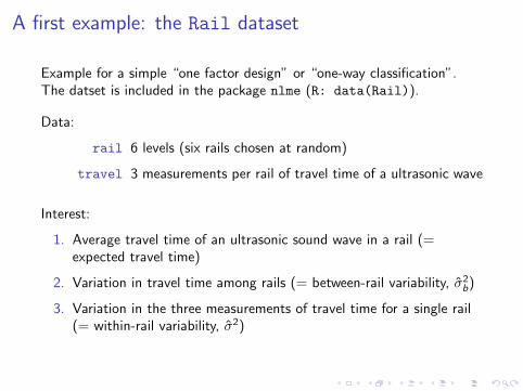
A first example: the Rail dataset
Example for a simple “one factor design” or “one-way classification”.The datset is included in the package nlme (R: data(Rail)).
Data:
rail 6 levels (six rails chosen at random)
travel 3 measurements per rail of travel time of a ultrasonic wave
Interest:
1. Average travel time of an ultrasonic sound wave in a rail (=expected travel time)
2. Variation in travel time among rails (= between-rail variability, σ2b)
3. Variation in the three measurements of travel time for a single rail(= within-rail variability, σ2)
A first example: the Rail dataset
Zero−force travel time (nanoseconds)
Rai
l
2
5
1
6
3
4
40 60 80 100
●●●
● ●●
● ●●
● ●●
● ●●
● ●●
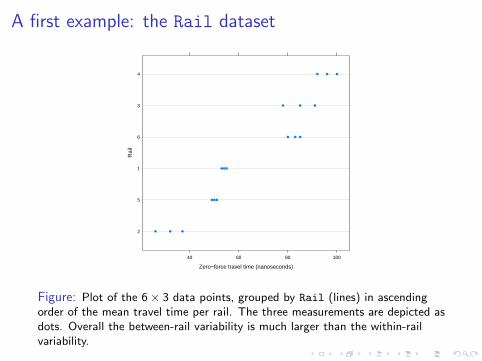
Figure: Plot of the 6× 3 data points, grouped by Rail (lines) in ascendingorder of the mean travel time per rail. The three measurements are depicted asdots. Overall the between-rail variability is much larger than the within-railvariability.
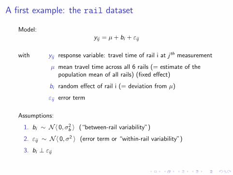
A first example: the rail dataset
Model:yij = µ+ bi + εij
with yij response variable: travel time of rail i at j th measurement
µ mean travel time across all 6 rails (= estimate of thepopulation mean of all rails) (fixed effect)
bi random effect of rail i (= deviation from µ)
εij error term
Assumptions:
1. bi ∼ N〈 0, σ2b 〉 (“between-rail variability”)
2. εij ∼ N〈 0, σ2 〉 (error term or “within-rail variability”)
3. bi ⊥ εij
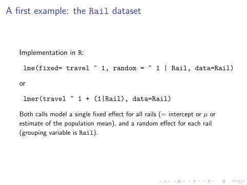
A first example: the Rail dataset
Implementation in R:
lme(fixed= travel ~ 1, random = ~ 1 | Rail, data=Rail)
or
lmer(travel ~ 1 + (1|Rail), data=Rail)
Both calls model a single fixed effect for all rails (= intercept or µ or
estimate of the population mean), and a random effect for each rail
(grouping variable is Rail).
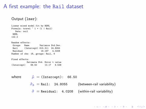
A first example: the Rail dataset
Output (lmer):
Linear mixed model fit by REML
Formula: travel ~ 1 + (1 | Rail)
Data: rail
REML
122.2
Random effects:
Groups Name Variance Std.Dev.
Rail (Intercept) 615.311 24.8055
Residual 16.167 4.0208
Number of obs: 18, groups: Rail, 6
Fixed effects:
Estimate Std. Error t value
(Intercept) 66.50 10.17 6.538
where µ = (Intercept): 66.50
σb = Rail: 24.8055 (between-rail variability)
σ = Residual: 4.0208 (within-rail variability)
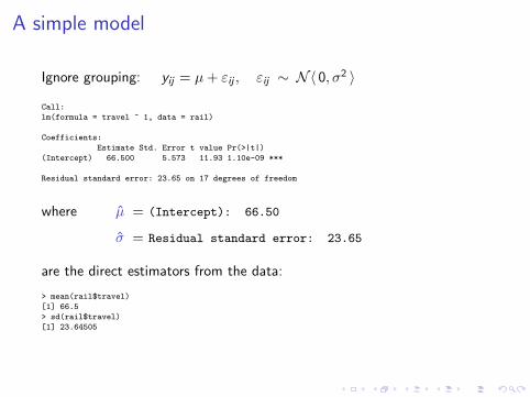
A simple model
Ignore grouping: yij = µ+ εij , εij ∼ N〈 0, σ2 〉
Call:
lm(formula = travel ~ 1, data = rail)
Coefficients:
Estimate Std. Error t value Pr(>|t|)
(Intercept) 66.500 5.573 11.93 1.10e-09 ***
Residual standard error: 23.65 on 17 degrees of freedom
where µ = (Intercept): 66.50
σ = Residual standard error: 23.65
are the direct estimators from the data:
> mean(rail$travel)
[1] 66.5
> sd(rail$travel)
[1] 23.64505
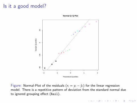
Is it a good model?
●
●
●
−2 −1 0 1 2
−40
−20
020
Normal Q−Q Plot
Theoretical Quantiles
Sam
ple
Qua
ntile
s
Figure: Normal-Plot of the residuals (ri = yi − yi ) for the linear regressionmodel. There is a repetitive pattern of deviation from the standard normal dueto ignored grouping effect (Rail).
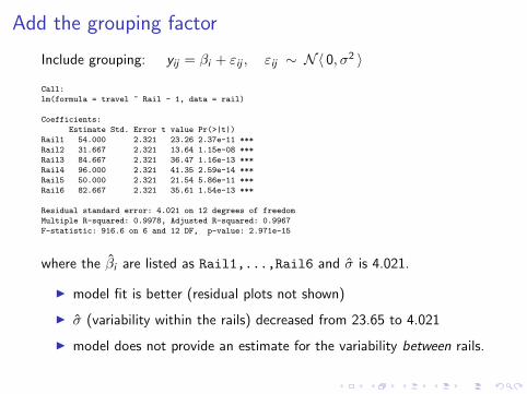
Add the grouping factor
Include grouping: yij = βi + εij , εij ∼ N〈 0, σ2 〉
Call:
lm(formula = travel ~ Rail - 1, data = rail)
Coefficients:
Estimate Std. Error t value Pr(>|t|)
Rail1 54.000 2.321 23.26 2.37e-11 ***
Rail2 31.667 2.321 13.64 1.15e-08 ***
Rail3 84.667 2.321 36.47 1.16e-13 ***
Rail4 96.000 2.321 41.35 2.59e-14 ***
Rail5 50.000 2.321 21.54 5.86e-11 ***
Rail6 82.667 2.321 35.61 1.54e-13 ***
Residual standard error: 4.021 on 12 degrees of freedom
Multiple R-squared: 0.9978, Adjusted R-squared: 0.9967
F-statistic: 916.6 on 6 and 12 DF, p-value: 2.971e-15
where the βi are listed as Rail1,...,Rail6 and σ is 4.021.
I model fit is better (residual plots not shown)
I σ (variability within the rails) decreased from 23.65 to 4.021
I model does not provide an estimate for the variability between rails.
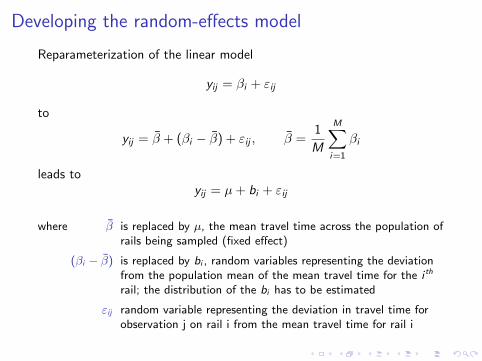
Developing the random-effects model
Reparameterization of the linear model
yij = βi + εij
to
yij = β + (βi − β) + εij , β =1
M
M∑i=1
βi
leads toyij = µ+ bi + εij
where β is replaced by µ, the mean travel time across the population ofrails being sampled (fixed effect)
(βi − β) is replaced by bi , random variables representing the deviationfrom the population mean of the mean travel time for the i th
rail; the distribution of the bi has to be estimated
εij random variable representing the deviation in travel time forobservation j on rail i from the mean travel time for rail i

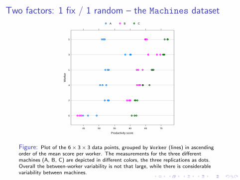
Two factors: 1 fix / 1 random – the Machines dataset
Example for a “replicated, randomized block design” with an interaction term.The dataset is included in the package nlme (R: data(Machines)).
Data:
score Productivity score achieved on a machine (measured 3 times)
Machine Type of machine used (3 levels)
Worker Subject used in the experiment (6 levels)
Interest:
1. Expected productivity score of the three different machines
2. Is there an interdependence of worker and machine?
3. Variation among workers (= between-worker variability, σ2b)
4. Variation within a worker (= within-worker variability, σ2)
Two factors: 1 fix / 1 random – the Machines dataset
Productivity score
Wor
ker
6
2
4
1
3
5
45 50 55 60 65 70
● ●●
● ●●
●●●
● ●●
● ●●
●● ●
● ● ●
●●●
●● ●
●●●
●●●
● ●●
●●●
●● ●
●●●
● ●●
●●●
●●●
● ● ●A B C
Figure: Plot of the 6× 3× 3 data points, grouped by Worker (lines) in ascendingorder of the mean score per worker. The measurements for the three differentmachines (A, B, C) are depicted in different colors, the three replications as dots.Overall the between-worker variability is not that large, while there is considerablevariability between machines.
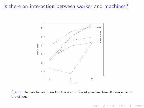
Is there an interaction between worker and machines?
4550
5560
6570
Machine
mea
n of
sco
re
A B C
Worker
531426
Figure: As can be seen, worker 6 scored differently on machine B compared tothe others.
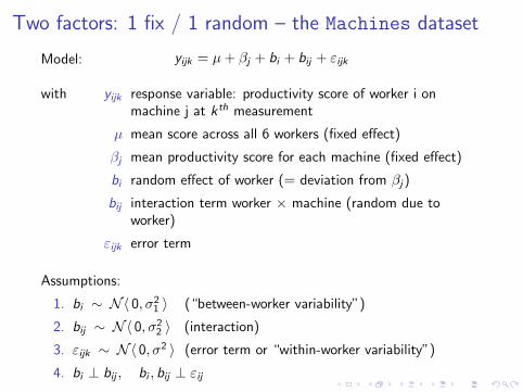
Two factors: 1 fix / 1 random – the Machines dataset
Model: yijk = µ+ βj + bi + bij + εijk
with yijk response variable: productivity score of worker i onmachine j at k th measurement
µ mean score across all 6 workers (fixed effect)
βj mean productivity score for each machine (fixed effect)
bi random effect of worker (= deviation from βj)
bij interaction term worker × machine (random due toworker)
εijk error term
Assumptions:
1. bi ∼ N〈 0, σ21 〉 (“between-worker variability”)
2. bij ∼ N〈 0, σ22 〉 (interaction)
3. εijk ∼ N〈 0, σ2 〉 (error term or “within-worker variability”)
4. bi ⊥ bij , bi , bij ⊥ εij
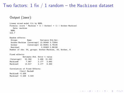
Two factors: 1 fix / 1 random – the Machines dataset
Output (lmer):
Linear mixed model fit by REML
Formula: score ~ Machine + (1 | Worker) + (1 | Worker:Machine)
Data: machine
REML
215.7
Random effects:
Groups Name Variance Std.Dev.
Worker:Machine (Intercept) 13.90945 3.72954
Worker (Intercept) 22.85851 4.78106
Residual 0.92463 0.96158
Number of obs: 54, groups: Worker:Machine, 18; Worker, 6
Fixed effects:
Estimate Std. Error t value
(Intercept) 52.356 2.486 21.062
MachineB 7.967 2.177 3.660
MachineC 13.917 2.177 6.393
Correlation of Fixed Effects:
(Intr) MachnB
MachineB -0.438
MachineC -0.438 0.500
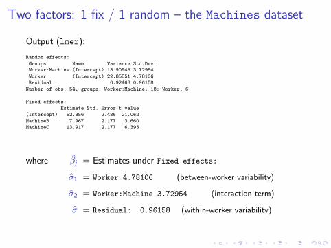
Two factors: 1 fix / 1 random – the Machines dataset
Output (lmer):
Random effects:
Groups Name Variance Std.Dev.
Worker:Machine (Intercept) 13.90945 3.72954
Worker (Intercept) 22.85851 4.78106
Residual 0.92463 0.96158
Number of obs: 54, groups: Worker:Machine, 18; Worker, 6
Fixed effects:
Estimate Std. Error t value
(Intercept) 52.356 2.486 21.062
MachineB 7.967 2.177 3.660
MachineC 13.917 2.177 6.393
where βj = Estimates under Fixed effects:
σ1 = Worker 4.78106 (between-worker variability)
σ2 = Worker:Machine 3.72954 (interaction term)
σ = Residual: 0.96158 (within-worker variability)

Two factors: both random – the manager1 dataset
Example for a model with two random effects in a crossed design. (Thedataset manager1 is constructed.)
Background A behavioural researcher has devised a method for evaluating“managerial style” by observing the ordinary workdayinteractions of managers and rating certain kinds ofoccurrences. Because the evaluation method is to be applied inthe field by many different evaluators, it is important to findout whether ratings vary much or little from one trainedevaluator to another.
Interest: Variation among raters (= between-rater variability) with themain question: “can the test be generalized”?
Design: Each rater evaluated all 20 managers (crossed design).
Data: score Score on an observational rating scale (measured once)
Rater (3 levels)
Manager Subject evaluated in the experiment (20 levels)
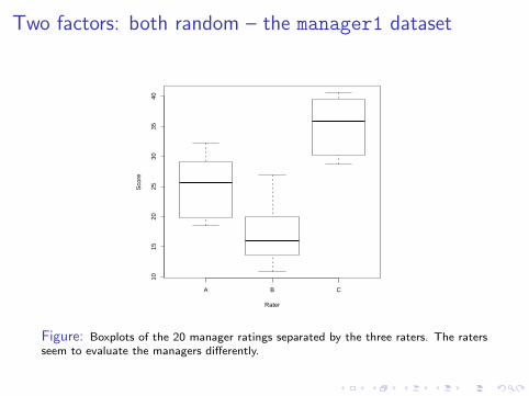
Two factors: both random – the manager1 dataset
A B C
1015
2025
3035
40
Rater
Sco
re
Figure: Boxplots of the 20 manager ratings separated by the three raters. The ratersseem to evaluate the managers differently.
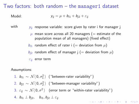
Two factors: both random – the manager1 dataset
Model: yij = µ+ bi1 + bj2 + εij
with yij response variable: score given by rater i for manager j
µ mean score across all 20 managers (= estimate of thepopulation mean of all managers) (fixed effect)
bi1 random effect of rater i (= deviation from µ)
bj2 random effect of manager j (= deviation from µ)
εij error term
Assumptions:
1. bi1 ∼ N〈 0, σ21 〉 (“between-rater variability”)
2. bj2 ∼ N〈 0, σ22 〉 (“between-manager variability”)
3. εij ∼ N〈 0, σ2 〉 (error term or “within-rater variability”)
4. bi1 ⊥ bj2, bi1, bj2 ⊥ εij
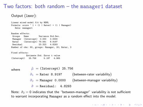
Two factors: both random – the manager1 dataset
Output (lmer):
Linear mixed model fit by REML
Formula: score ~ 1 + (1 | Rater) + (1 | Manager)
Data: manager1
Random effects:
Groups Name Variance Std.Dev.
Manager (Intercept) 0.000 0.0000
Rater (Intercept) 79.561 8.9197
Residual 23.323 4.8293
Number of obs: 60, groups: Manager, 20; Rater, 3
Fixed effects:
Estimate Std. Error t value
(Intercept) 25.756 5.187 4.965
where µ = (Intercept) 25.756
σ1 = Rater 8.9197 (between-rater variability)
σ2 = Manager 0.0000 (between-manager variability)
σ = Residual: 4.8293
Note: σ2 = 0 indicates that the “between-manager” variability is not sufficientto warrant incorporating Manager as a random effect into the model.
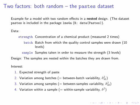
Two factors: both random – the pastes dataset
Example for a model with two random effects in a nested design. (The datasetpastes is included in the package lme4a (R: data(Pastes)).
Data:
strength Concentration of a chemical product (measured 2 times)
batch Batch from which the quality control samples were drawn (10levels)
sample Samples taken in order to measure the strength (3 levels)
Design: The samples are nested within the batches they are drawn from.
Interest:
1. Expected strength of paste
2. Variation among batches (= between-batch variability, σ2b1)
3. Variation among samples (= between-samples variability, σ2b2)
4. Variation within a sample (= within-sample variability, σ2)
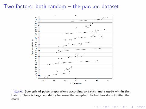
Two factors: both random – the pastes dataset
Figure: Strength of paste preparations according to batch and sample within thebatch. There is large variability between the samples, the batches do not differ thatmuch.
Two factors: both random – the pastes dataset
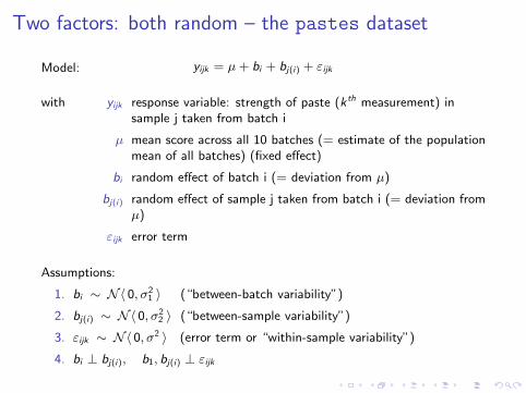
Model: yijk = µ+ bi + bj(i) + εijk
with yijk response variable: strength of paste (k th measurement) insample j taken from batch i
µ mean score across all 10 batches (= estimate of the populationmean of all batches) (fixed effect)
bi random effect of batch i (= deviation from µ)
bj(i) random effect of sample j taken from batch i (= deviation fromµ)
εijk error term
Assumptions:
1. bi ∼ N〈 0, σ21 〉 (“between-batch variability”)
2. bj(i) ∼ N〈 0, σ22 〉 (“between-sample variability”)
3. εijk ∼ N〈 0, σ2 〉 (error term or “within-sample variability”)
4. bi ⊥ bj(i), b1, bj(i) ⊥ εijk
Two factors: both random – the pastes dataset
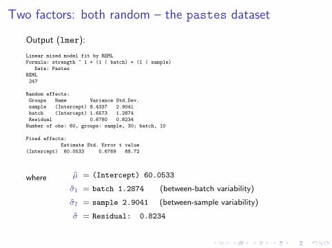
Output (lmer):
Linear mixed model fit by REML
Formula: strength ~ 1 + (1 | batch) + (1 | sample)
Data: Pastes
REML
247
Random effects:
Groups Name Variance Std.Dev.
sample (Intercept) 8.4337 2.9041
batch (Intercept) 1.6573 1.2874
Residual 0.6780 0.8234
Number of obs: 60, groups: sample, 30; batch, 10
Fixed effects:
Estimate Std. Error t value
(Intercept) 60.0533 0.6769 88.72
where µ = (Intercept) 60.0533
σ1 = batch 1.2874 (between-batch variability)
σ2 = sample 2.9041 (between-sample variability)
σ = Residual: 0.8234
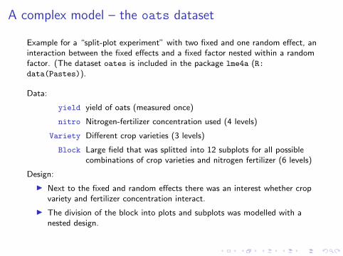
A complex model – the oats dataset
Example for a “split-plot experiment” with two fixed and one random effect, aninteraction between the fixed effects and a fixed factor nested within a randomfactor. (The dataset oates is included in the package lme4a (R:data(Pastes)).
Data:
yield yield of oats (measured once)
nitro Nitrogen-fertilizer concentration used (4 levels)
Variety Different crop varieties (3 levels)
Block Large field that was splitted into 12 subplots for all possiblecombinations of crop varieties and nitrogen fertilizer (6 levels)
Design:
I Next to the fixed and random effects there was an interest whether cropvariety and fertilizer concentration interact.
I The division of the block into plots and subplots was modelled with anested design.
A complex model – the oats dataset
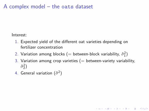
Interest:
1. Expected yield of the different oat varieties depending onfertilizer concentration
2. Variation among blocks (= between-block variability, σ21)
3. Variation among crop varieties (= between-variety variability,σ2
2)
4. General variation (σ2)
A complex model – the oats dataset
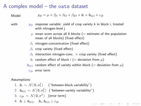
Model: yijk = µ+ βj1 + βk2 + βjk3 + bi + bk(i) + εijk
with yijk response variable: yield of crop variety k in block i, treatedwith nitrogen-level j
µ mean score across all 6 blocks (= estimate of the populationmean of all blocks) (fixed effect)
β1 nitrogen-concentration (fixed effect)
β2 crop variety (fixed effect)
β3 interaction nitrogen-conc. × crop variety (fixed effect)
bi random effect of block i (= deviation from µ)
bk(i) random effect of variety within block (= deviation from µ)
εijk error term
Assumptions:
1. bi ∼ N〈 0, σ21 〉 (“between-block variability”)
2. bk(i) ∼ N〈 0, σ22 〉 (“between-variety variability”)
3. εijk ∼ N〈 0, σ2 〉 (error term)
4. bi ⊥ bk(i), b1, bk(i) ⊥ εijk
A complex model – the oats dataset
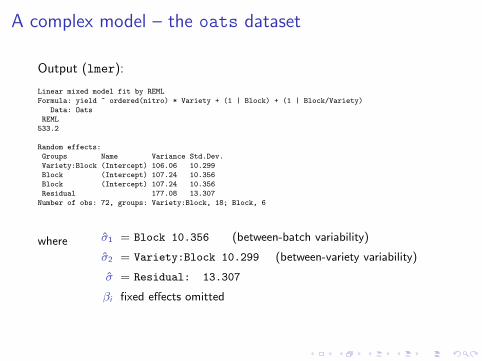
Output (lmer):
Linear mixed model fit by REML
Formula: yield ~ ordered(nitro) * Variety + (1 | Block) + (1 | Block/Variety)
Data: Oats
REML
533.2
Random effects:
Groups Name Variance Std.Dev.
Variety:Block (Intercept) 106.06 10.299
Block (Intercept) 107.24 10.356
Block (Intercept) 107.24 10.356
Residual 177.08 13.307
Number of obs: 72, groups: Variety:Block, 18; Block, 6
where σ1 = Block 10.356 (between-batch variability)
σ2 = Variety:Block 10.299 (between-variety variability)
σ = Residual: 13.307
βi fixed effects omitted