Introduction to Convex Optimizationhelper.ipam.ucla.edu/publications/gss2013/gss2013_11378.pdf1....
82
Introduction to Convex Optimization Lieven Vandenberghe Electrical Engineering Department, UCLA IPAM Graduate Summer School: Computer Vision August 5, 2013
Transcript of Introduction to Convex Optimizationhelper.ipam.ucla.edu/publications/gss2013/gss2013_11378.pdf1....
Introduction to Convex Optimization
Lieven Vandenberghe
Electrical Engineering Department, UCLA
IPAM Graduate Summer School: Computer Vision
August 5, 2013
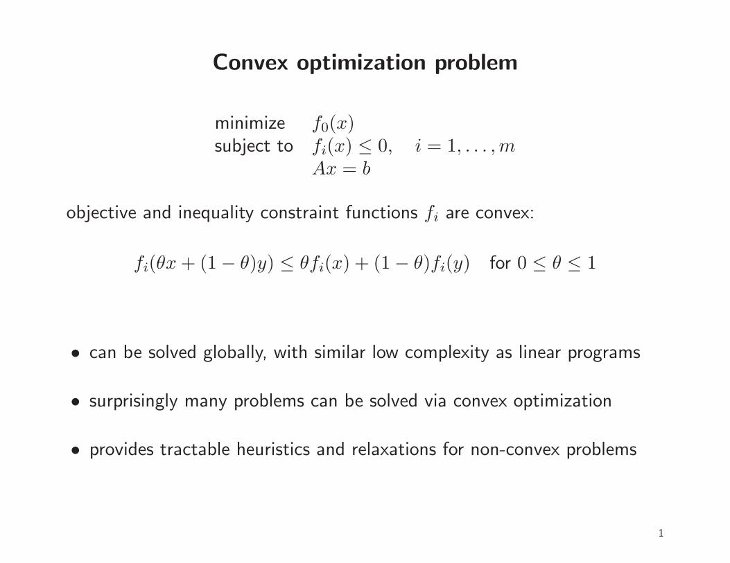
Convex optimization problem
minimize f0(x)subject to fi(x) ≤ 0, i = 1, . . . ,m
Ax = b
objective and inequality constraint functions fi are convex:
fi(θx+ (1− θ)y) ≤ θfi(x) + (1− θ)fi(y) for 0 ≤ θ ≤ 1
• can be solved globally, with similar low complexity as linear programs
• surprisingly many problems can be solved via convex optimization
• provides tractable heuristics and relaxations for non-convex problems
1

History
• 1940s: linear programming
minimize cTxsubject to aTi x ≤ bi, i = 1, . . . ,m
• 1950s: quadratic programming
minimize (1/2)xTPx+ qTxsubject to aTi x ≤ bi, i = 1, . . . ,m
• 1960s: geometric programming
• since 1990: semidefinite programming, second-order cone programming,quadratically constrained quadratic programming, robust optimization,sum-of-squares programming, . . .
2
New applications since 1990
• linear matrix inequality techniques in control
• semidefinite programming relaxations in combinatorial optimization
• support vector machine training via quadratic programming
• circuit design via geometric programming
• ℓ1-norm optimization for sparse signal reconstruction
• applications in structural optimization, statistics, machine learning,signal processing, communications, image processing, computer vision,quantum information theory, finance, power distribution, . . .
3
Advances in convex optimization algorithms
Interior-point methods
• 1984 (Karmarkar): first practical polynomial-time algorithm for LP
• 1984-1990: efficient implementations for large-scale LPs
• around 1990 (Nesterov & Nemirovski): polynomial-time interior-pointmethods for nonlinear convex programming
• 1990s: high-quality software packages for conic optimization
• 2000s: convex modeling software based on interior-point solvers
First-order algorithms
• fast gradient methods, based on Nesterov’s methods from 1980s
• extensions to nondifferentiable or constrained problems
• multiplier/splitting methods for large-scale and distributed optimization
4
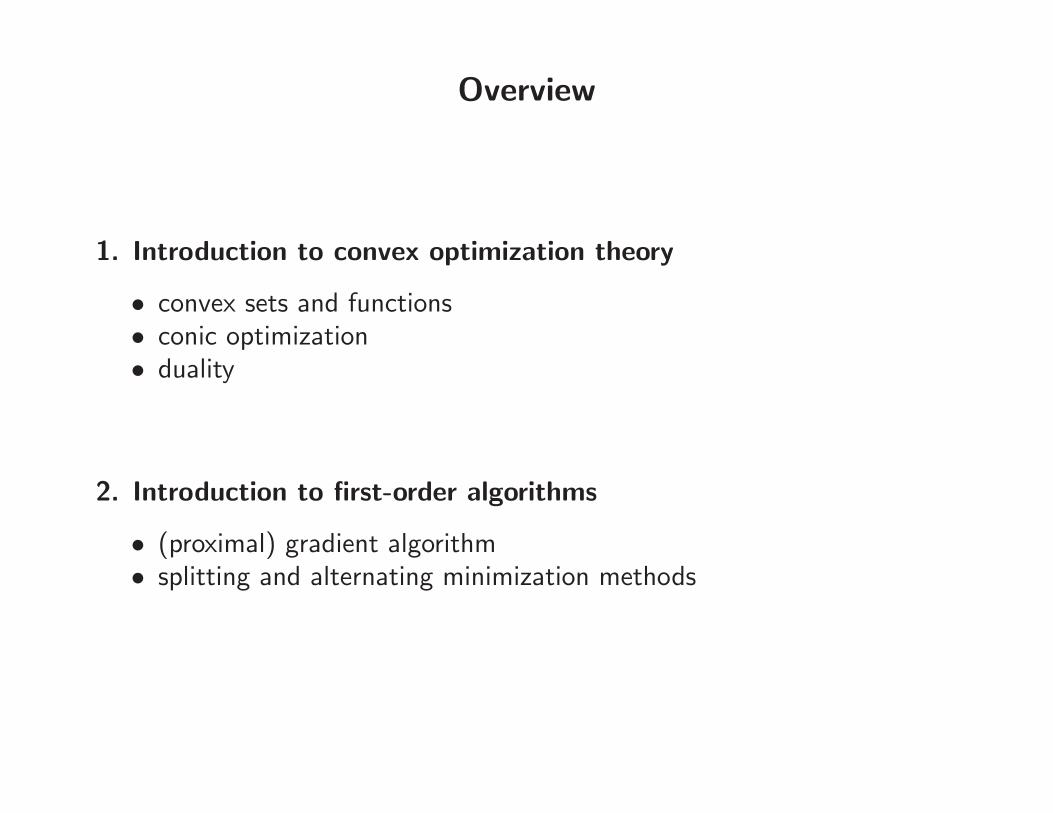
Overview
1. Introduction to convex optimization theory
• convex sets and functions• conic optimization• duality
2. Introduction to first-order algorithms
• (proximal) gradient algorithm• splitting and alternating minimization methods
2013 IPAM Graduate Summer School: Computer Vision
1. Convex optimization theory
• convex sets and functions
• conic optimization
• duality
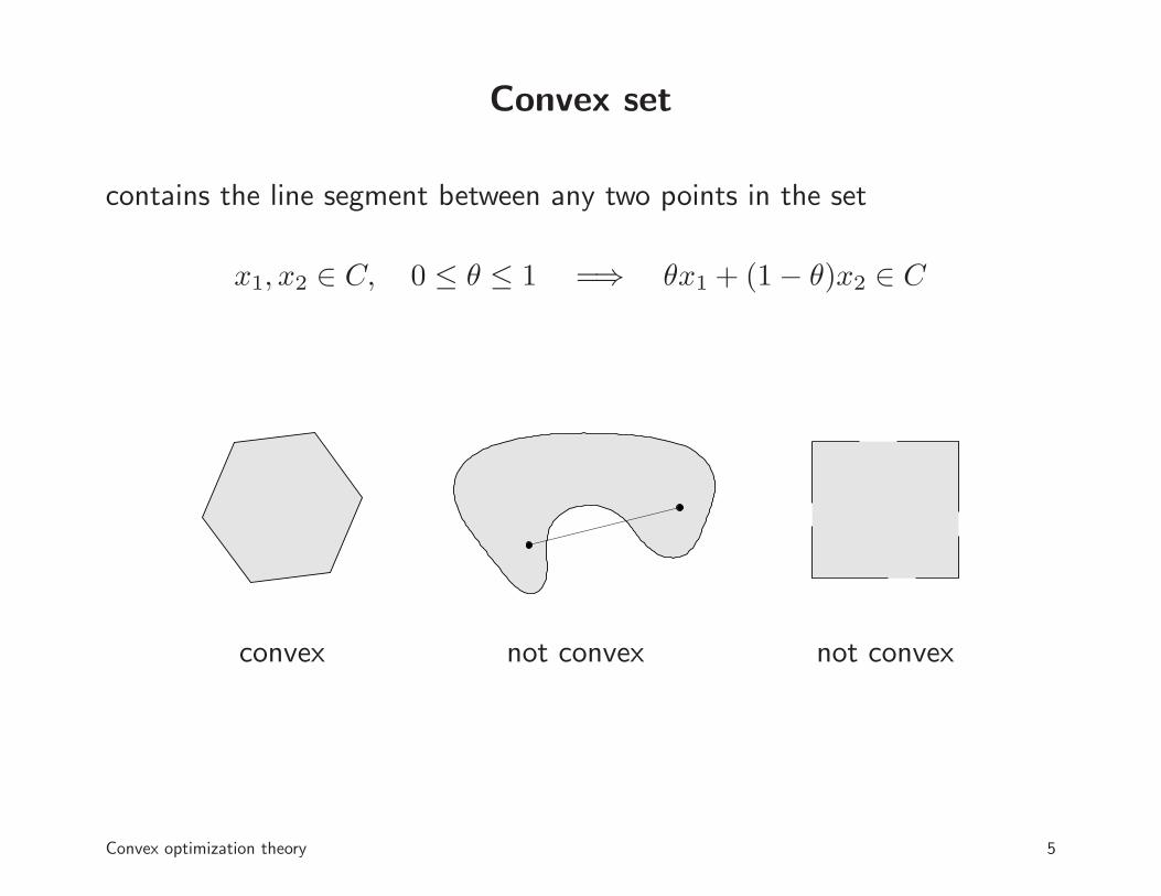
Convex set
contains the line segment between any two points in the set
x1, x2 ∈ C, 0 ≤ θ ≤ 1 =⇒ θx1 + (1− θ)x2 ∈ C
convex not convex not convex
Convex optimization theory 5
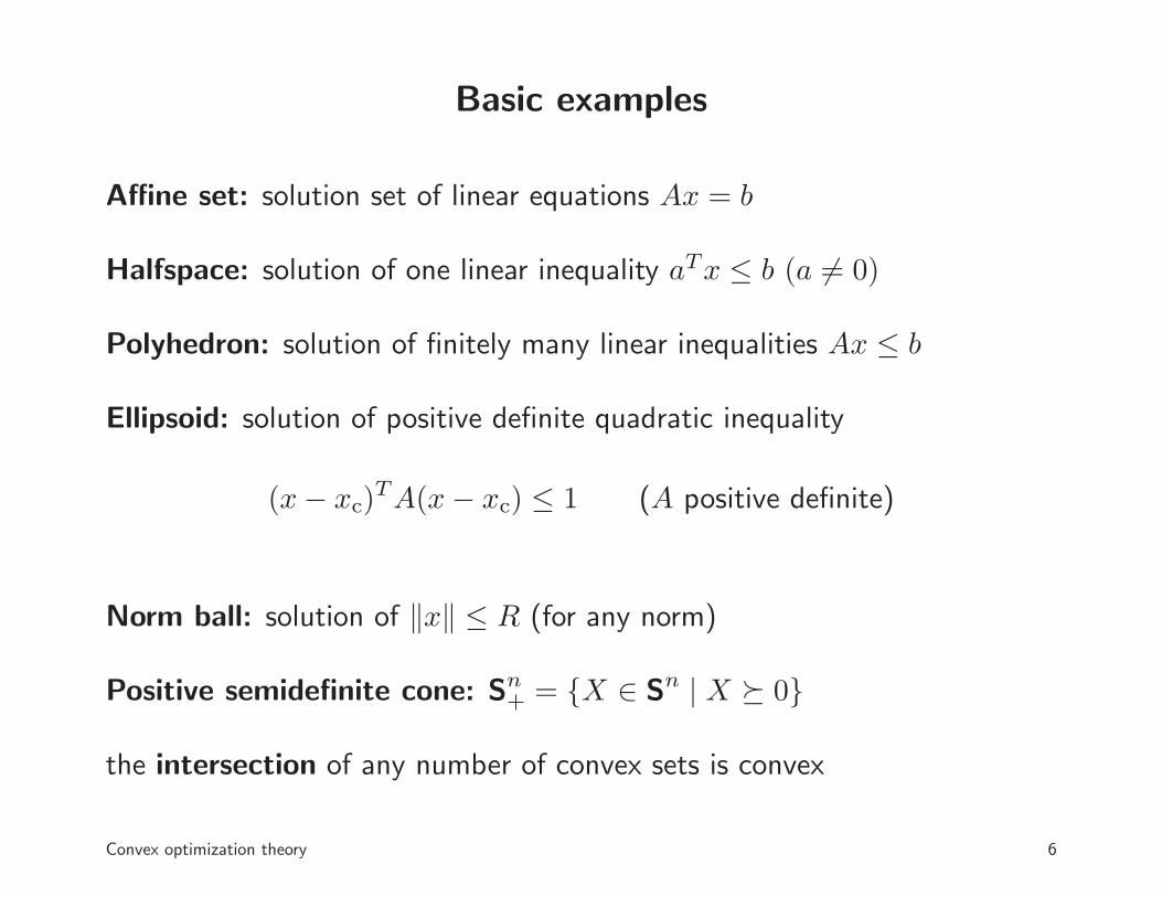
Basic examples
Affine set: solution set of linear equations Ax = b
Halfspace: solution of one linear inequality aTx ≤ b (a 6= 0)
Polyhedron: solution of finitely many linear inequalities Ax ≤ b
Ellipsoid: solution of positive definite quadratic inequality
(x− xc)TA(x− xc) ≤ 1 (A positive definite)
Norm ball: solution of ‖x‖ ≤ R (for any norm)
Positive semidefinite cone: Sn+ = {X ∈ Sn | X � 0}
the intersection of any number of convex sets is convex
Convex optimization theory 6
Convex function
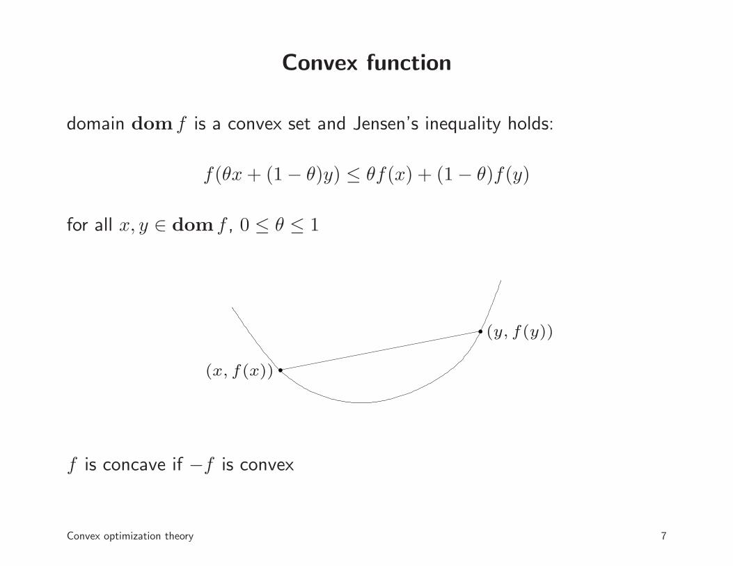
domain dom f is a convex set and Jensen’s inequality holds:
f(θx+ (1− θ)y) ≤ θf(x) + (1− θ)f(y)
for all x, y ∈ dom f , 0 ≤ θ ≤ 1
(x, f(x))
(y, f(y))
f is concave if −f is convex
Convex optimization theory 7
Examples
• linear and affine functions are convex and concave
• expx, − log x, x log x are convex
• xα is convex for x > 0 and α ≥ 1 or α ≤ 0; |x|α is convex for α ≥ 1
• norms are convex
• quadratic-over-linear function xTx/t is convex in x, t for t > 0
• geometric mean (x1x2 · · ·xn)1/n is concave for x ≥ 0
• log detX is concave on set of positive definite matrices
• log(ex1 + · · · exn) is convex
Convex optimization theory 8
Differentiable convex functions
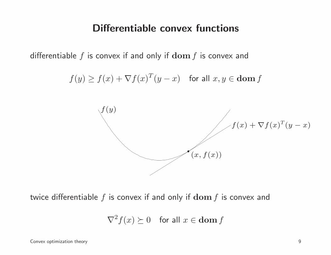
differentiable f is convex if and only if dom f is convex and
f(y) ≥ f(x) +∇f(x)T (y − x) for all x, y ∈ dom f
(x, f(x))
f(y)
f(x) + ∇f(x)T (y − x)
twice differentiable f is convex if and only if dom f is convex and
∇2f(x) � 0 for all x ∈ dom f
Convex optimization theory 9
Subgradient
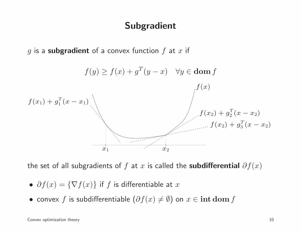
g is a subgradient of a convex function f at x if
f(y) ≥ f(x) + gT (y − x) ∀y ∈ dom f
x1 x2
f(x1) + gT1 (x − x1)
f(x2) + gT2 (x − x2)
f(x2) + gT3 (x − x2)
f(x)
the set of all subgradients of f at x is called the subdifferential ∂f(x)
• ∂f(x) = {∇f(x)} if f is differentiable at x
• convex f is subdifferentiable (∂f(x) 6= ∅) on x ∈ int dom f
Convex optimization theory 10
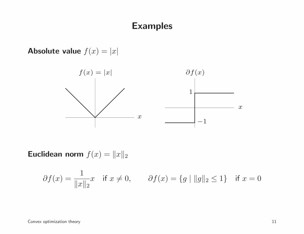
Examples
Absolute value f(x) = |x|
f(x) = |x| ∂f(x)
x
x
1
−1
Euclidean norm f(x) = ‖x‖2
∂f(x) =1
‖x‖2x if x 6= 0, ∂f(x) = {g | ‖g‖2 ≤ 1} if x = 0
Convex optimization theory 11
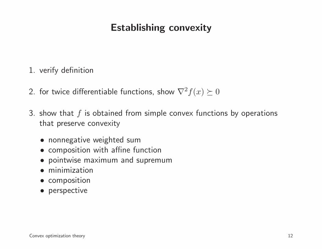
Establishing convexity
1. verify definition
2. for twice differentiable functions, show ∇2f(x) � 0
3. show that f is obtained from simple convex functions by operationsthat preserve convexity
• nonnegative weighted sum• composition with affine function• pointwise maximum and supremum• minimization• composition• perspective
Convex optimization theory 12
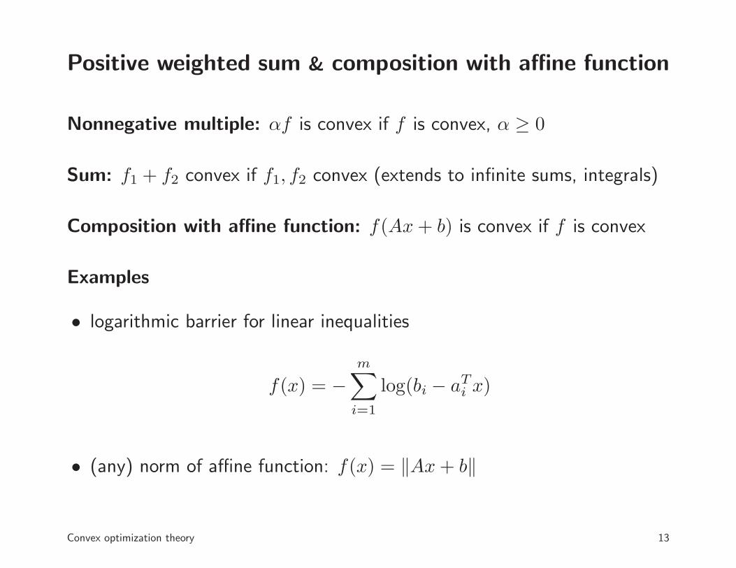
Positive weighted sum & composition with affine function
Nonnegative multiple: αf is convex if f is convex, α ≥ 0
Sum: f1 + f2 convex if f1, f2 convex (extends to infinite sums, integrals)
Composition with affine function: f(Ax+ b) is convex if f is convex
Examples
• logarithmic barrier for linear inequalities
f(x) = −m∑
i=1
log(bi − aTi x)
• (any) norm of affine function: f(x) = ‖Ax+ b‖
Convex optimization theory 13
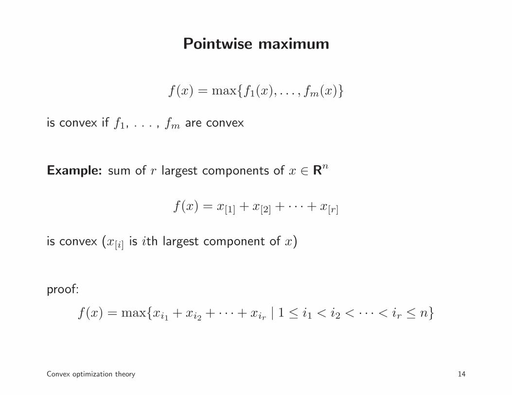
Pointwise maximum
f(x) = max{f1(x), . . . , fm(x)}
is convex if f1, . . . , fm are convex
Example: sum of r largest components of x ∈ Rn
f(x) = x[1] + x[2] + · · ·+ x[r]
is convex (x[i] is ith largest component of x)
proof:
f(x) = max{xi1 + xi2 + · · ·+ xir | 1 ≤ i1 < i2 < · · · < ir ≤ n}
Convex optimization theory 14
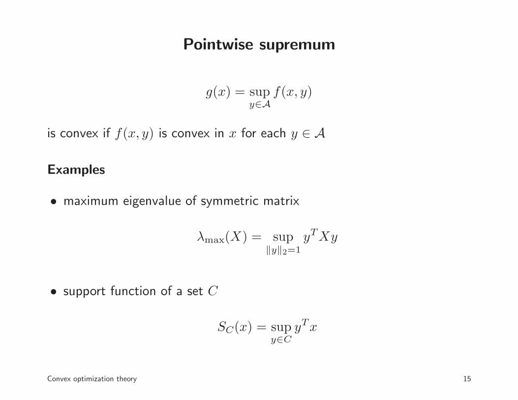
Pointwise supremum
g(x) = supy∈A
f(x, y)
is convex if f(x, y) is convex in x for each y ∈ A
Examples
• maximum eigenvalue of symmetric matrix
λmax(X) = sup‖y‖2=1
yTXy
• support function of a set C
SC(x) = supy∈C
yTx
Convex optimization theory 15
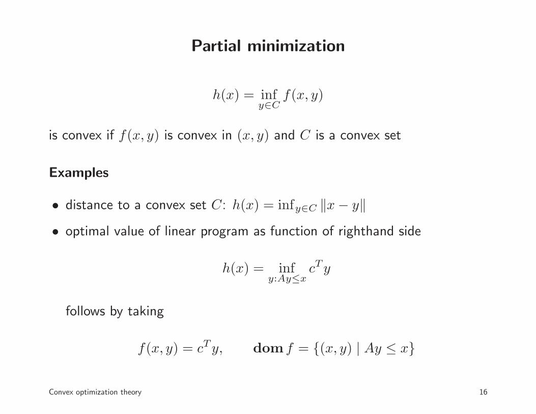
Partial minimization
h(x) = infy∈C
f(x, y)
is convex if f(x, y) is convex in (x, y) and C is a convex set
Examples
• distance to a convex set C: h(x) = infy∈C ‖x− y‖• optimal value of linear program as function of righthand side
h(x) = infy:Ay≤x
cTy
follows by taking
f(x, y) = cTy, dom f = {(x, y) | Ay ≤ x}
Convex optimization theory 16
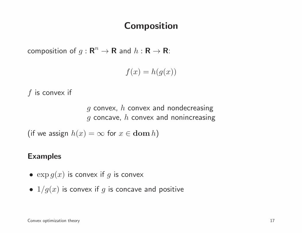
Composition
composition of g : Rn → R and h : R → R:
f(x) = h(g(x))
f is convex if
g convex, h convex and nondecreasingg concave, h convex and nonincreasing
(if we assign h(x) = ∞ for x ∈ domh)
Examples
• exp g(x) is convex if g is convex
• 1/g(x) is convex if g is concave and positive
Convex optimization theory 17
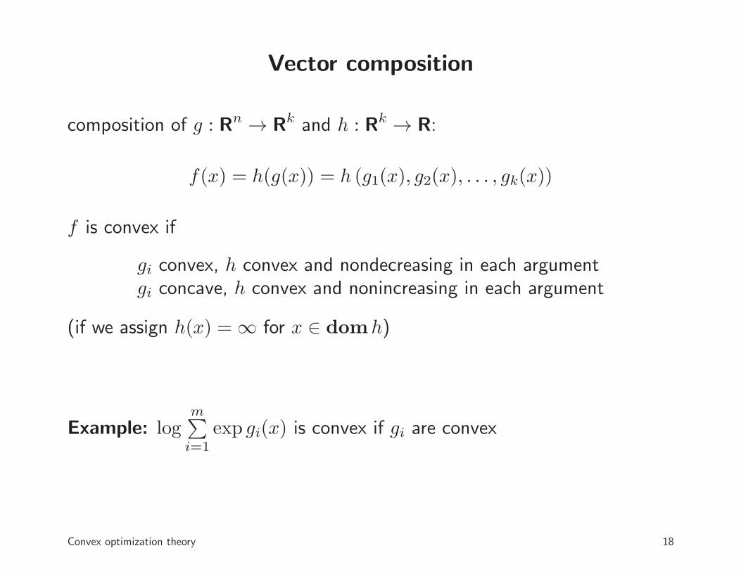
Vector composition
composition of g : Rn → Rk and h : Rk → R:
f(x) = h(g(x)) = h (g1(x), g2(x), . . . , gk(x))
f is convex if
gi convex, h convex and nondecreasing in each argumentgi concave, h convex and nonincreasing in each argument
(if we assign h(x) = ∞ for x ∈ domh)
Example: logm∑
i=1
exp gi(x) is convex if gi are convex
Convex optimization theory 18
Perspective
the perspective of a function f : Rn → R is the function g : Rn ×R → R,
g(x, t) = tf(x/t)
g is convex if f is convex on dom g = {(x, t) | x/t ∈ dom f, t > 0}
Examples
• perspective of f(x) = xTx is quadratic-over-linear function
g(x, t) =xTx
t
• perspective of negative logarithm f(x) = − log x is relative entropy
g(x, t) = t log t− t log x
Convex optimization theory 19
Modeling software
Modeling packages for convex optimization
• CVX, YALMIP (MATLAB)
• CVXPY, CVXMOD (Python)
• MOSEK Fusion (several platforms)
assist the user in formulating convex problems, by automating two tasks:
• verifying convexity from convex calculus rules
• transforming problem in input format required by standard solvers
Related packages
general-purpose optimization modeling: AMPL, GAMS
Convex optimization theory 20
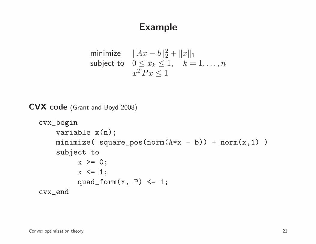
Example
minimize ‖Ax− b‖22 + ‖x‖1subject to 0 ≤ xk ≤ 1, k = 1, . . . , n
xTPx ≤ 1
CVX code (Grant and Boyd 2008)
cvx_begin
variable x(n);
minimize( square_pos(norm(A*x - b)) + norm(x,1) )
subject to
x >= 0;
x <= 1;
quad_form(x, P) <= 1;
cvx_end
Convex optimization theory 21
Outline
• convex sets and functions
• conic optimization
• duality
Conic linear program
minimize cTxsubject to b−Ax ∈ K
• K a convex cone (closed, pointed, with nonempty interior)
• if K is the nonnegative orthant, this is a (regular) linear program
• constraint often written as generalized linear inequality Ax �K b
widely used in recent literature on convex optimization
• modeling: 3 cones (nonnegative orthant, second-order cone, positivesemidefinite cone) are sufficient to represent most convex constraints
• algorithms: a convenient problem format when extending interior-pointalgorithms for linear programming to convex optimization
Convex optimization theory 22
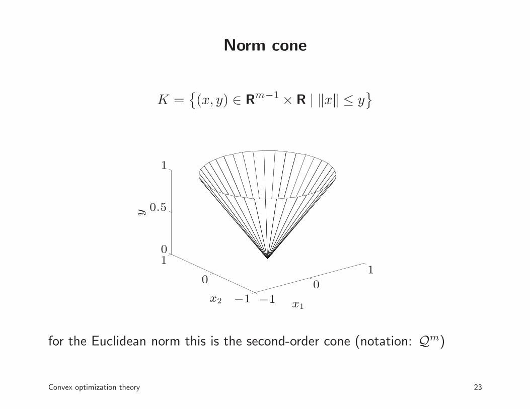
Norm cone
K ={(x, y) ∈ Rm−1 × R | ‖x‖ ≤ y
}
x1x2
y
−1
0
1
−1
0
10
0.5
1
for the Euclidean norm this is the second-order cone (notation: Qm)
Convex optimization theory 23
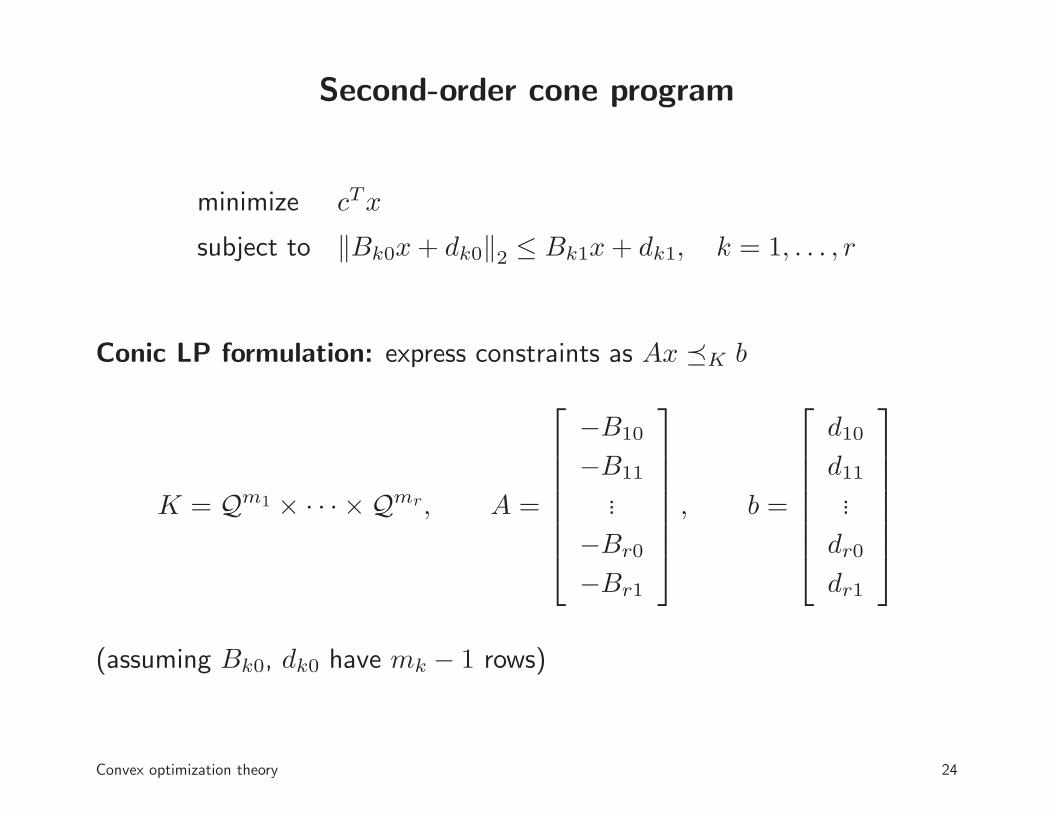
Second-order cone program
minimize cTx
subject to ‖Bk0x+ dk0‖2 ≤ Bk1x+ dk1, k = 1, . . . , r
Conic LP formulation: express constraints as Ax �K b
K = Qm1 × · · · × Qmr, A =
−B10
−B11
...
−Br0
−Br1
, b =
d10
d11...
dr0
dr1
(assuming Bk0, dk0 have mk − 1 rows)
Convex optimization theory 24
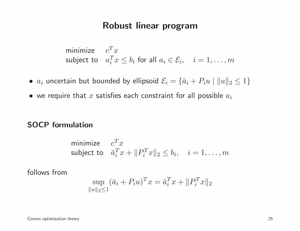
Robust linear program
minimize cTxsubject to aTi x ≤ bi for all ai ∈ Ei, i = 1, . . . ,m
• ai uncertain but bounded by ellipsoid Ei = {ai + Piu | ‖u‖2 ≤ 1}• we require that x satisfies each constraint for all possible ai
SOCP formulation
minimize cTxsubject to aTi x+ ‖PT
i x‖2 ≤ bi, i = 1, . . . ,m
follows fromsup
‖u‖2≤1
(ai + Piu)Tx = aTi x+ ‖PT
i x‖2
Convex optimization theory 25
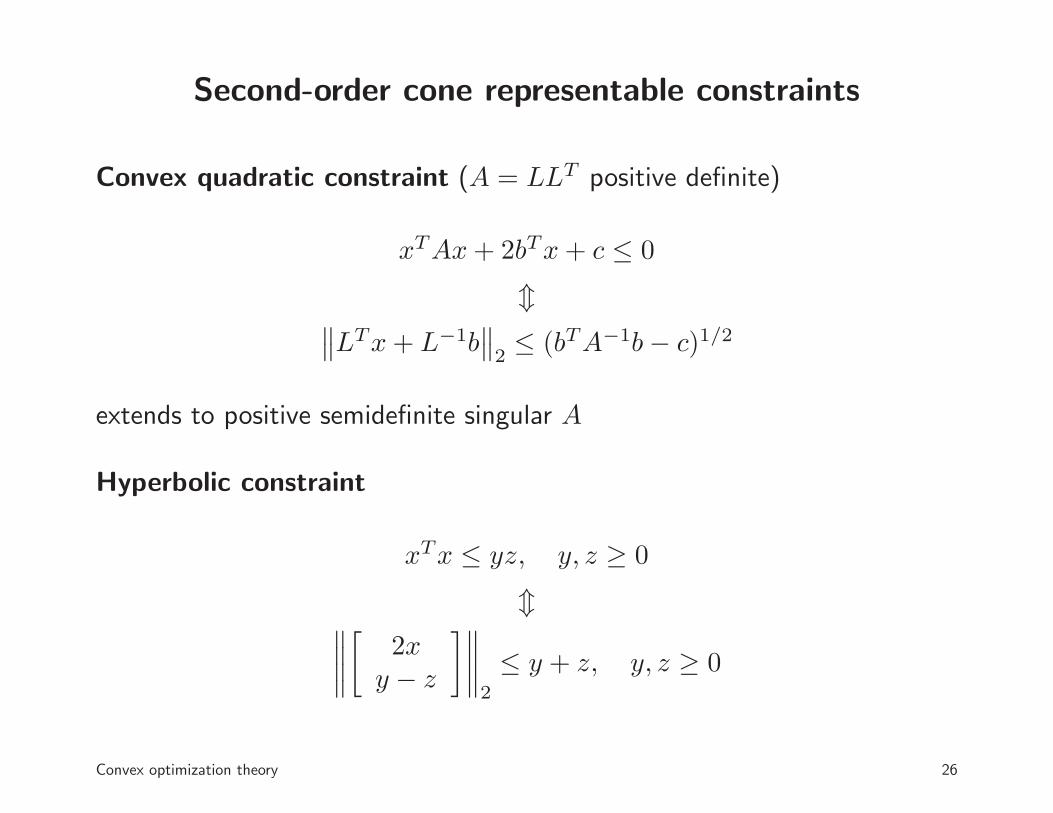
Second-order cone representable constraints
Convex quadratic constraint (A = LLT positive definite)
xTAx+ 2bTx+ c ≤ 0
m∥∥LTx+ L−1b
∥∥2≤ (bTA−1b− c)1/2
extends to positive semidefinite singular A
Hyperbolic constraint
xTx ≤ yz, y, z ≥ 0
m∥∥∥∥
[2x
y − z
]∥∥∥∥2
≤ y + z, y, z ≥ 0
Convex optimization theory 26
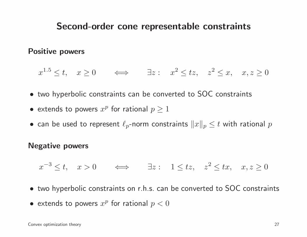
Second-order cone representable constraints
Positive powers
x1.5 ≤ t, x ≥ 0 ⇐⇒ ∃z : x2 ≤ tz, z2 ≤ x, x, z ≥ 0
• two hyperbolic constraints can be converted to SOC constraints
• extends to powers xp for rational p ≥ 1
• can be used to represent ℓp-norm constraints ‖x‖p ≤ t with rational p
Negative powers
x−3 ≤ t, x > 0 ⇐⇒ ∃z : 1 ≤ tz, z2 ≤ tx, x, z ≥ 0
• two hyperbolic constraints on r.h.s. can be converted to SOC constraints
• extends to powers xp for rational p < 0
Convex optimization theory 27
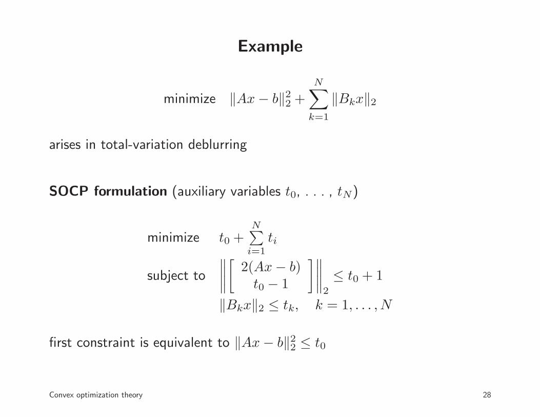
Example
minimize ‖Ax− b‖22 +N∑
k=1
‖Bkx‖2
arises in total-variation deblurring
SOCP formulation (auxiliary variables t0, . . . , tN)
minimize t0 +N∑
i=1
ti
subject to
∥∥∥∥
[2(Ax− b)t0 − 1
]∥∥∥∥2
≤ t0 + 1
‖Bkx‖2 ≤ tk, k = 1, . . . , N
first constraint is equivalent to ‖Ax− b‖22 ≤ t0
Convex optimization theory 28
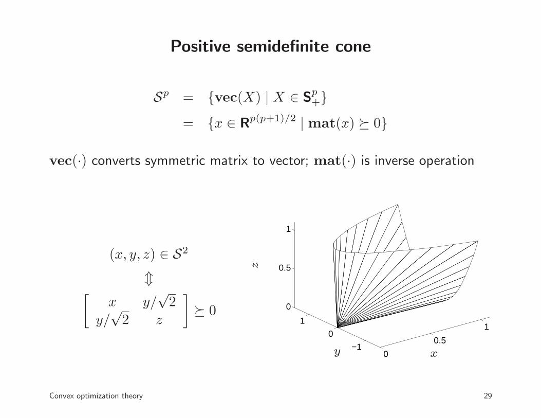
Positive semidefinite cone
Sp = {vec(X) | X ∈ Sp+}
= {x ∈ Rp(p+1)/2 | mat(x) � 0}
vec(·) converts symmetric matrix to vector; mat(·) is inverse operation
(x, y, z) ∈ S2
m[
x y/√2
y/√2 z
]
� 0
0
0.5
1
−1
0
1
0
0.5
1
xy
z
Convex optimization theory 29
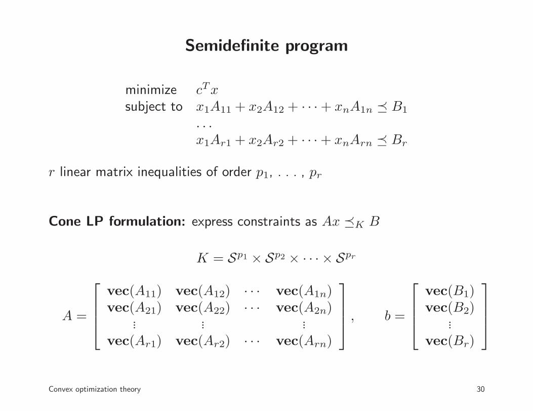
Semidefinite program
minimize cTxsubject to x1A11 + x2A12 + · · ·+ xnA1n � B1
. . .x1Ar1 + x2Ar2 + · · ·+ xnArn � Br
r linear matrix inequalities of order p1, . . . , pr
Cone LP formulation: express constraints as Ax �K B
K = Sp1 × Sp2 × · · · × Spr
A =
vec(A11) vec(A12) · · · vec(A1n)vec(A21) vec(A22) · · · vec(A2n)
... ... ...vec(Ar1) vec(Ar2) · · · vec(Arn)
, b =
vec(B1)vec(B2)
...vec(Br)
Convex optimization theory 30

Semidefinite cone representable constraints
Matrix-fractional function
yTX−1y ≤ t, X ≻ 0, y ∈ range(X)
m[
X yyT t
]
� 0
Maximum eigenvalue of symmetric matrix
λmax(X) ≤ t ⇐⇒ X � tI
Convex optimization theory 31
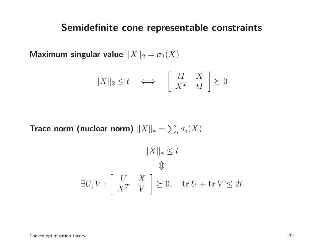
Semidefinite cone representable constraints
Maximum singular value ‖X‖2 = σ1(X)
‖X‖2 ≤ t ⇐⇒[
tI XXT tI
]
� 0
Trace norm (nuclear norm) ‖X‖∗ =∑
i σi(X)
‖X‖∗ ≤ t
m
∃U, V :
[U XXT V
]
� 0, trU + trV ≤ 2t
Convex optimization theory 32
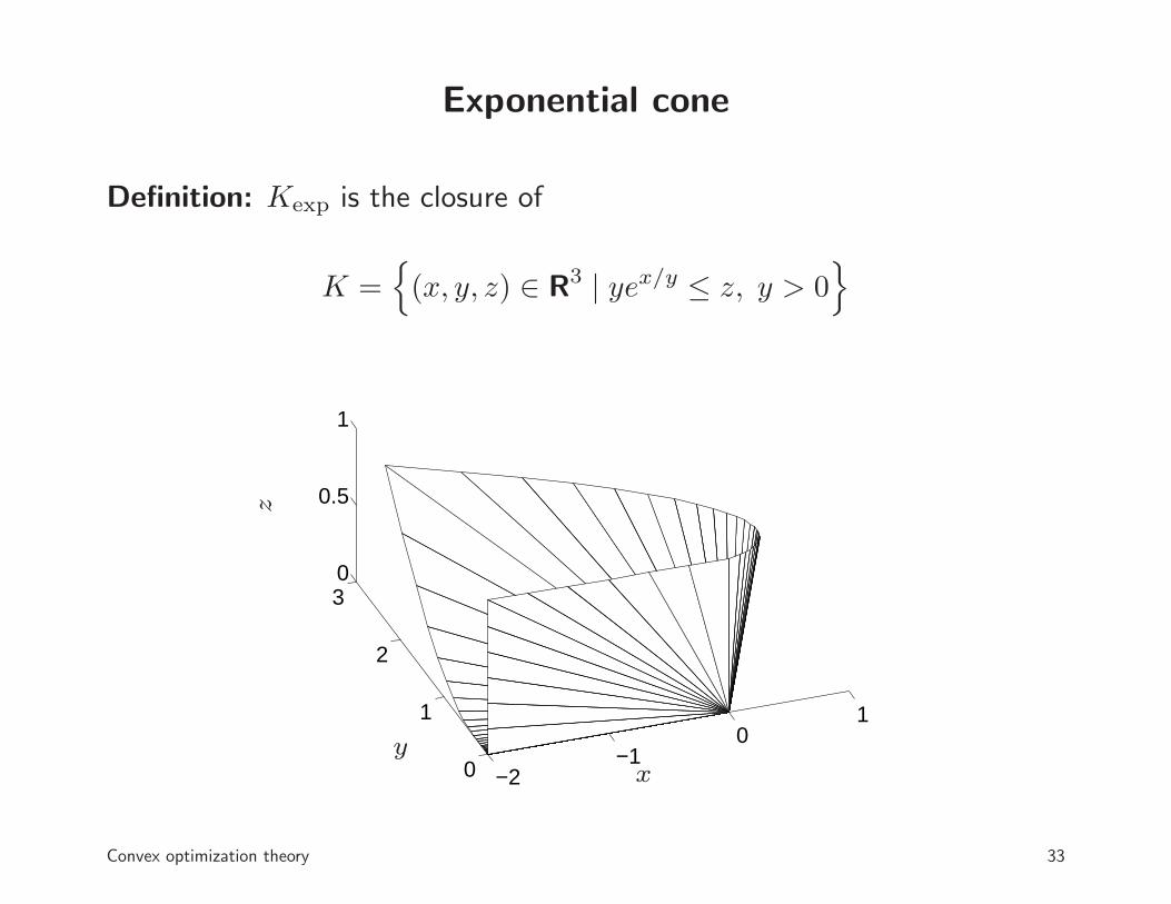
Exponential cone
Definition: Kexp is the closure of
K ={
(x, y, z) ∈ R3 | yex/y ≤ z, y > 0}
−2−1
01
0
1
2
30
0.5
1
xy
z
Convex optimization theory 33
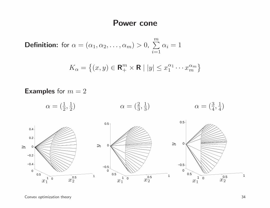
Power cone
Definition: for α = (α1, α2, . . . , αm) > 0,m∑
i=1
αi = 1
Kα ={(x, y) ∈ Rm
+ × R | |y| ≤ xα11 · · ·xαm
m
}
Examples for m = 2
α = (12,12) α = (23,
13) α = (34,
14)
00.5
1 0 0.5 1
−0.4
−0.2
0
0.2
0.4
x1 x2
y
00.5
1 0 0.5 1
−0.5
0
0.5
x1 x2
y
00.5
1 0 0.5 1
−0.5
0
0.5
x1 x2
y
Convex optimization theory 34
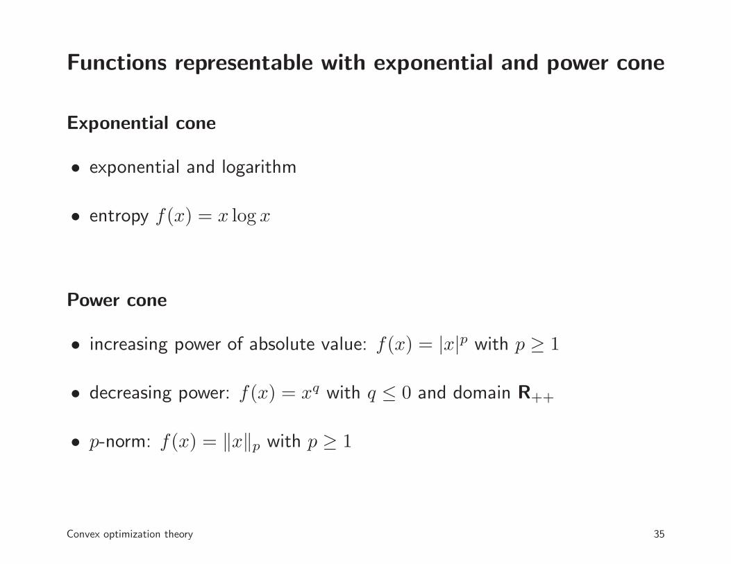
Functions representable with exponential and power cone
Exponential cone
• exponential and logarithm
• entropy f(x) = x log x
Power cone
• increasing power of absolute value: f(x) = |x|p with p ≥ 1
• decreasing power: f(x) = xq with q ≤ 0 and domain R++
• p-norm: f(x) = ‖x‖p with p ≥ 1
Convex optimization theory 35
Outline
• convex sets and functions
• conic optimization
• duality
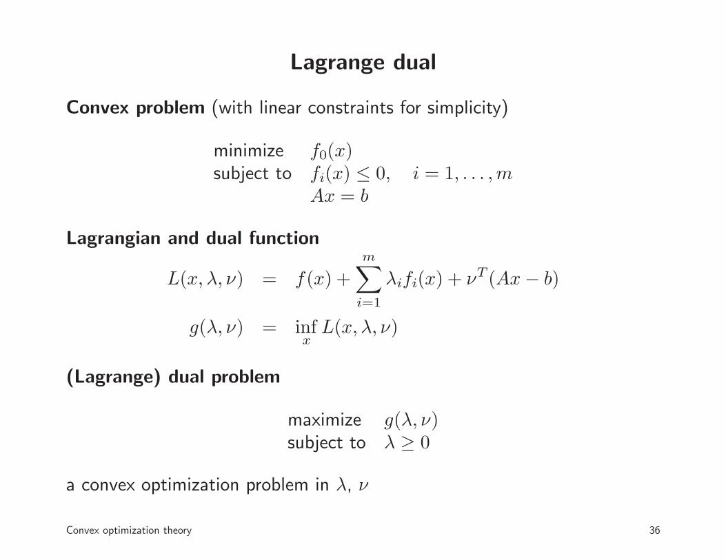
Lagrange dual
Convex problem (with linear constraints for simplicity)
minimize f0(x)subject to fi(x) ≤ 0, i = 1, . . . ,m
Ax = b
Lagrangian and dual function
L(x, λ, ν) = f(x) +
m∑
i=1
λifi(x) + νT (Ax− b)
g(λ, ν) = infx
L(x, λ, ν)
(Lagrange) dual problem
maximize g(λ, ν)subject to λ ≥ 0
a convex optimization problem in λ, ν
Convex optimization theory 36
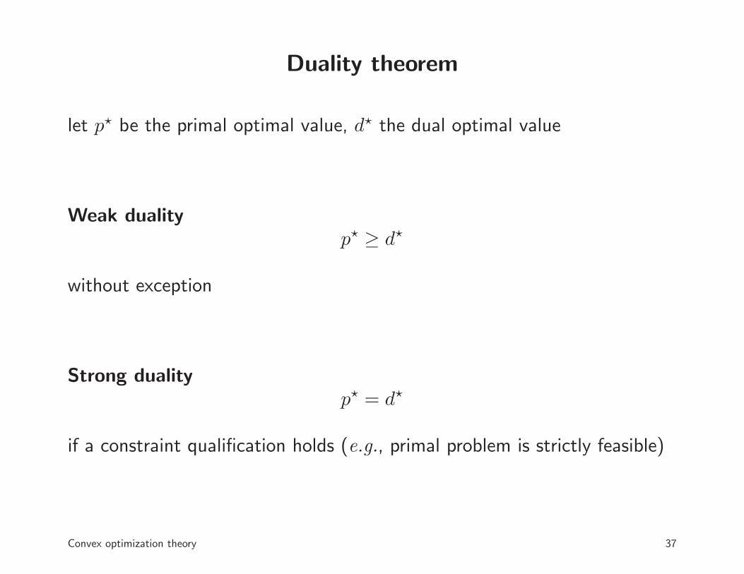
Duality theorem
let p⋆ be the primal optimal value, d⋆ the dual optimal value
Weak dualityp⋆ ≥ d⋆
without exception
Strong dualityp⋆ = d⋆
if a constraint qualification holds (e.g., primal problem is strictly feasible)
Convex optimization theory 37
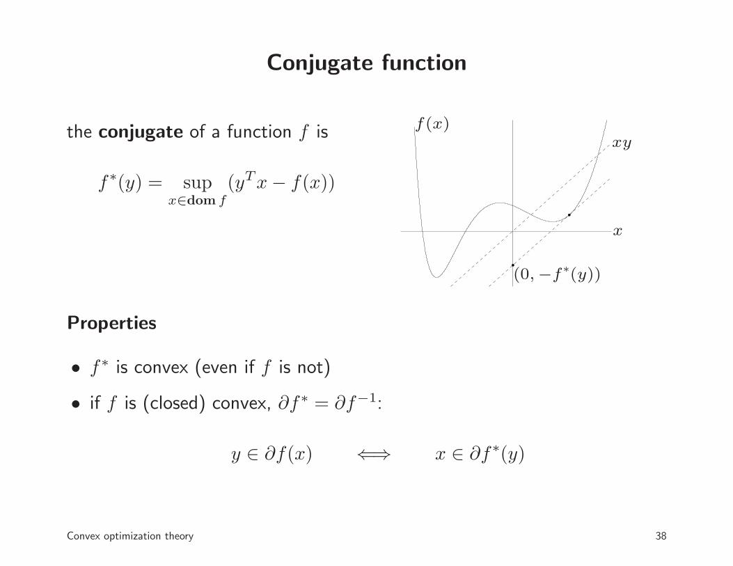
Conjugate function
the conjugate of a function f is
f∗(y) = supx∈dom f
(yTx− f(x))
f(x)
(0,−f∗(y))
xy
x
Properties
• f∗ is convex (even if f is not)
• if f is (closed) convex, ∂f∗ = ∂f−1:
y ∈ ∂f(x) ⇐⇒ x ∈ ∂f∗(y)
Convex optimization theory 38
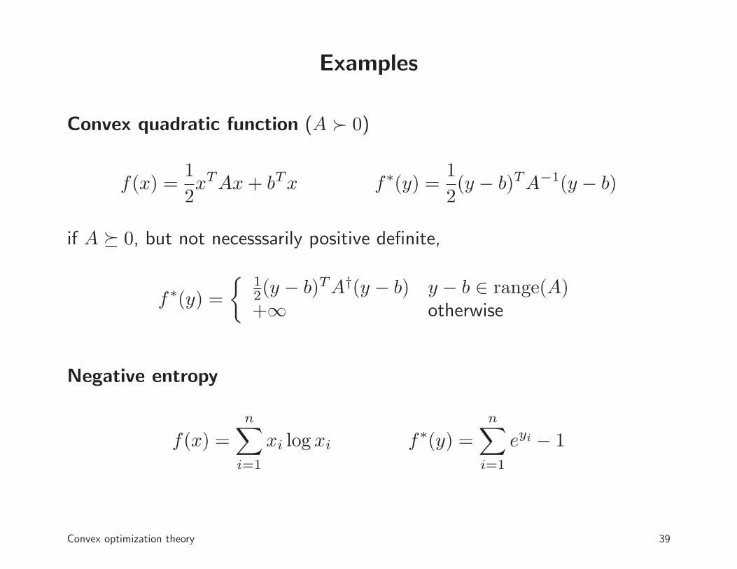
Examples
Convex quadratic function (A ≻ 0)
f(x) =1
2xTAx+ bTx f∗(y) =
1
2(y − b)TA−1(y − b)
if A � 0, but not necesssarily positive definite,
f∗(y) =
{12(y − b)TA†(y − b) y − b ∈ range(A)+∞ otherwise
Negative entropy
f(x) =
n∑
i=1
xi log xi f∗(y) =
n∑
i=1
eyi − 1
Convex optimization theory 39
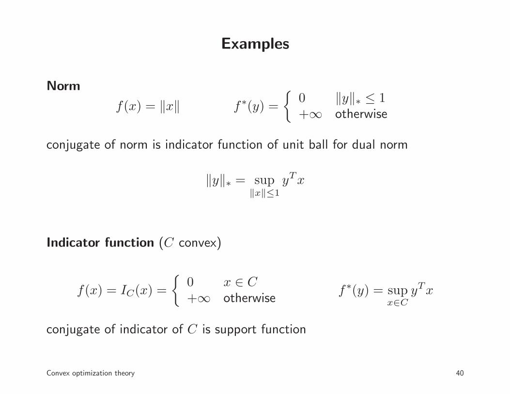
Examples
Norm
f(x) = ‖x‖ f∗(y) =
{0 ‖y‖∗ ≤ 1+∞ otherwise
conjugate of norm is indicator function of unit ball for dual norm
‖y‖∗ = sup‖x‖≤1
yTx
Indicator function (C convex)
f(x) = IC(x) =
{0 x ∈ C+∞ otherwise
f∗(y) = supx∈C
yTx
conjugate of indicator of C is support function
Convex optimization theory 40
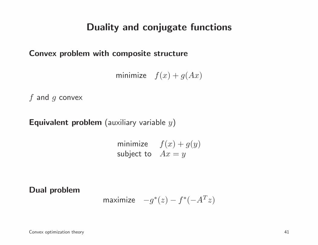
Duality and conjugate functions
Convex problem with composite structure
minimize f(x) + g(Ax)
f and g convex
Equivalent problem (auxiliary variable y)
minimize f(x) + g(y)subject to Ax = y
Dual problemmaximize −g∗(z)− f∗(−ATz)
Convex optimization theory 41
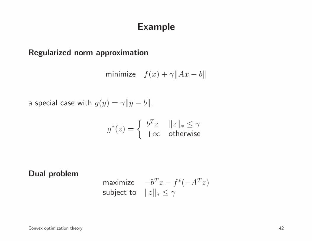
Example
Regularized norm approximation
minimize f(x) + γ‖Ax− b‖
a special case with g(y) = γ‖y − b‖,
g∗(z) =
{bTz ‖z‖∗ ≤ γ+∞ otherwise
Dual problemmaximize −bTz − f∗(−ATz)subject to ‖z‖∗ ≤ γ
Convex optimization theory 42
2013 IPAM Graduate Summer School: Computer Vision
2. First-order methods
• (proximal) gradient method
• splitting and alternating minimization methods
43

Proximal operator
the proximal operator (prox-operator) of a convex function h is
proxh(x) = argminu
(
h(u) +1
2‖u− x‖22
)
• h(x) = 0: proxh(x) = x
• h(x) = IC(x) (indicator function of C): proxh is projection on C
proxh(x) = argminu∈C
‖u− x‖22 = PC(x)
• h(x) = ‖x‖1: proxh is the ‘soft-threshold’ (shrinkage) operation
proxh(x)i =
xi − 1 xi ≥ 10 |xi| ≤ 1xi + 1 xi ≤ −1
First-order methods 44
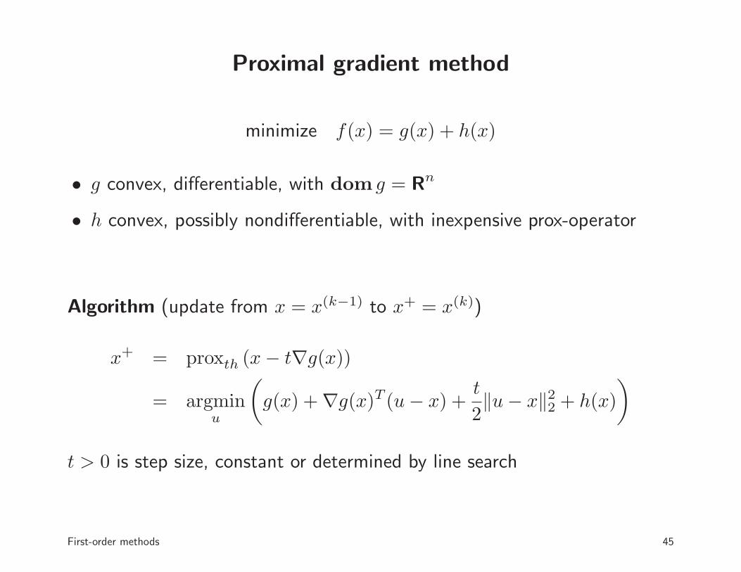
Proximal gradient method
minimize f(x) = g(x) + h(x)
• g convex, differentiable, with dom g = Rn
• h convex, possibly nondifferentiable, with inexpensive prox-operator
Algorithm (update from x = x(k−1) to x+ = x(k))
x+ = proxth (x− t∇g(x))
= argminu
(
g(x) +∇g(x)T (u− x) +t
2‖u− x‖22 + h(x)
)
t > 0 is step size, constant or determined by line search
First-order methods 45
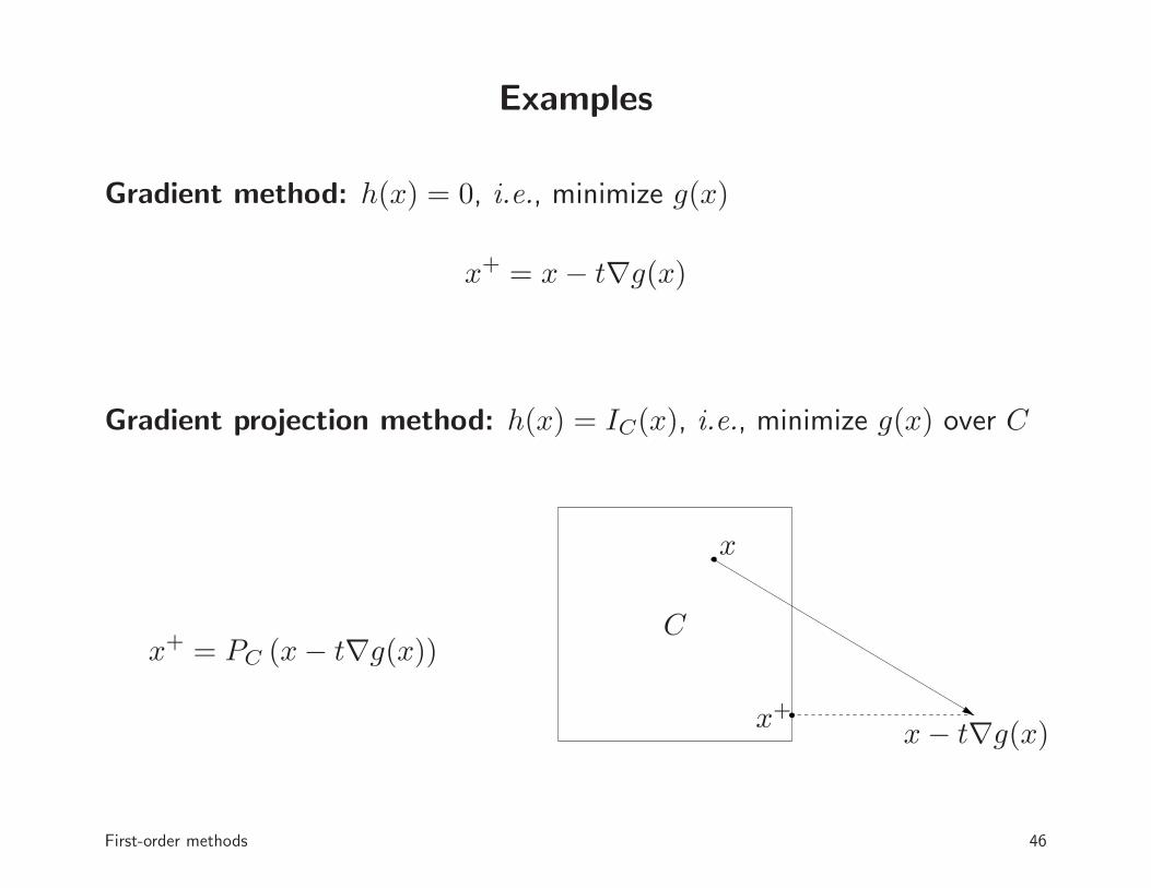
Examples
Gradient method: h(x) = 0, i.e., minimize g(x)
x+ = x− t∇g(x)
Gradient projection method: h(x) = IC(x), i.e., minimize g(x) over C
x+ = PC (x− t∇g(x))C
x
x− t∇g(x)x+
First-order methods 46
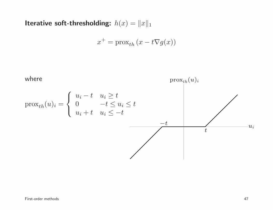
Iterative soft-thresholding: h(x) = ‖x‖1
x+ = proxth (x− t∇g(x))
where
proxth(u)i =
ui − t ui ≥ t0 −t ≤ ui ≤ tui + t ui ≤ −t
uit
−t
proxth(u)i
First-order methods 47
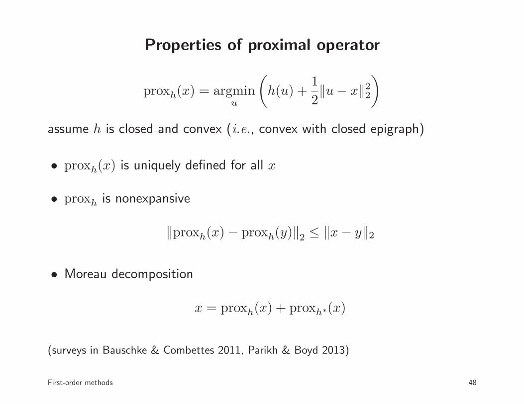
Properties of proximal operator
proxh(x) = argminu
(
h(u) +1
2‖u− x‖22
)
assume h is closed and convex (i.e., convex with closed epigraph)
• proxh(x) is uniquely defined for all x
• proxh is nonexpansive
‖proxh(x)− proxh(y)‖2 ≤ ‖x− y‖2
• Moreau decomposition
x = proxh(x) + proxh∗(x)
(surveys in Bauschke & Combettes 2011, Parikh & Boyd 2013)
First-order methods 48
Examples of inexpensive projections
• hyperplanes and halfspaces
• rectangles{x | l ≤ x ≤ u}
• probability simplex{x | 1Tx = 1, x ≥ 0}
• norm ball for many norms (Euclidean, 1-norm, . . . )
• nonnegative orthant, second-order cone, positive semidefinite cone
First-order methods 49
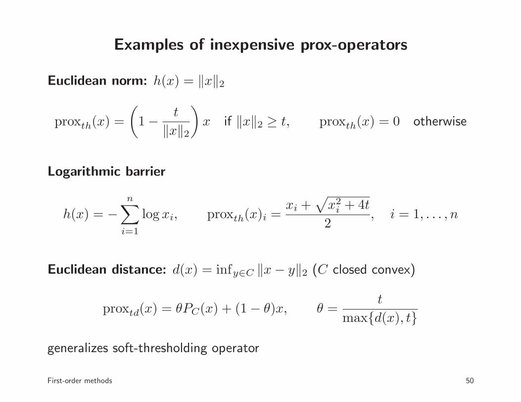
Examples of inexpensive prox-operators
Euclidean norm: h(x) = ‖x‖2
proxth(x) =
(
1− t
‖x‖2
)
x if ‖x‖2 ≥ t, proxth(x) = 0 otherwise
Logarithmic barrier
h(x) = −n∑
i=1
log xi, proxth(x)i =xi +
√
x2i + 4t
2, i = 1, . . . , n
Euclidean distance: d(x) = infy∈C ‖x− y‖2 (C closed convex)
proxtd(x) = θPC(x) + (1− θ)x, θ =t
max{d(x), t}
generalizes soft-thresholding operator
First-order methods 50
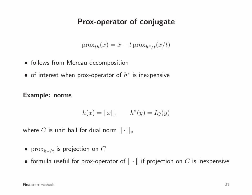
Prox-operator of conjugate
proxth(x) = x− t proxh∗/t(x/t)
• follows from Moreau decomposition
• of interest when prox-operator of h∗ is inexpensive
Example: norms
h(x) = ‖x‖, h∗(y) = IC(y)
where C is unit ball for dual norm ‖ · ‖∗
• proxh∗/t is projection on C
• formula useful for prox-operator of ‖ · ‖ if projection on C is inexpensive
First-order methods 51
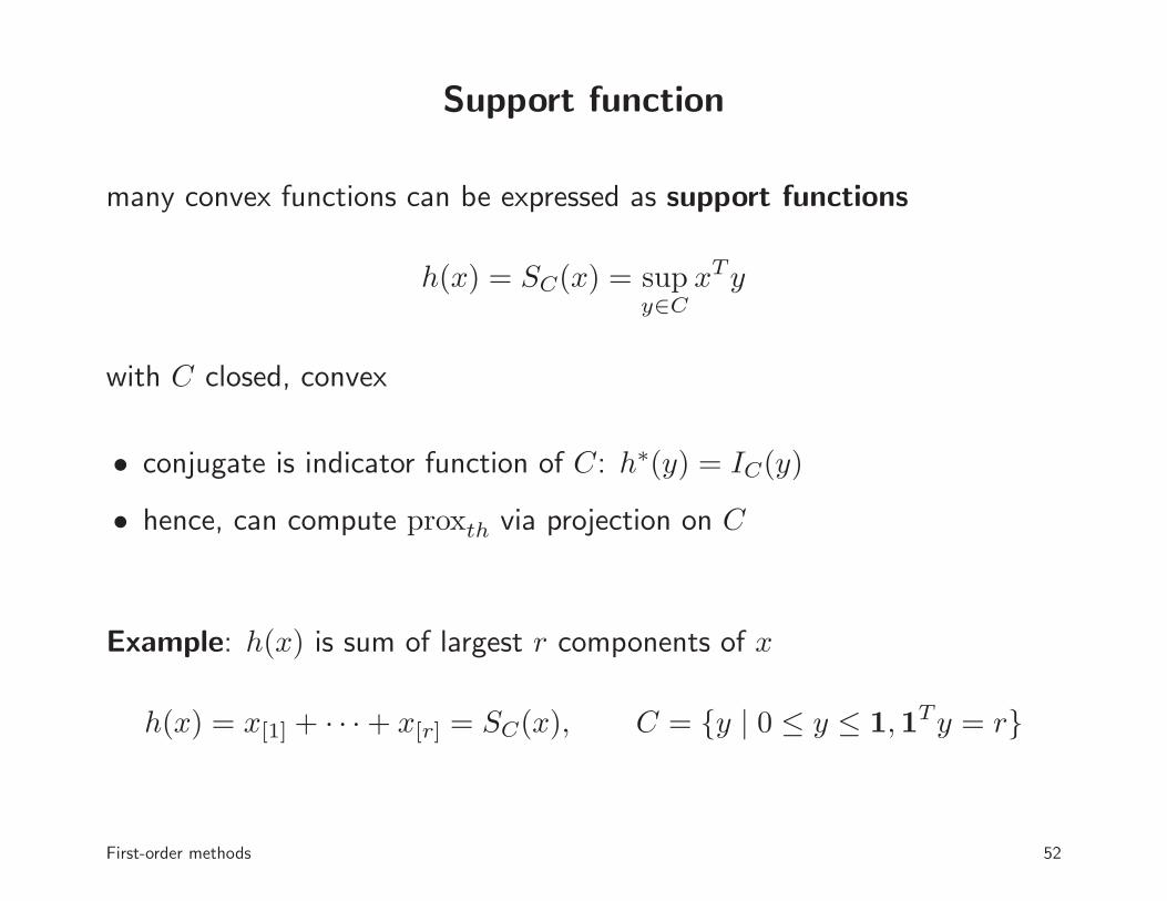
Support function
many convex functions can be expressed as support functions
h(x) = SC(x) = supy∈C
xTy
with C closed, convex
• conjugate is indicator function of C: h∗(y) = IC(y)
• hence, can compute proxth via projection on C
Example: h(x) is sum of largest r components of x
h(x) = x[1] + · · ·+ x[r] = SC(x), C = {y | 0 ≤ y ≤ 1,1Ty = r}
First-order methods 52
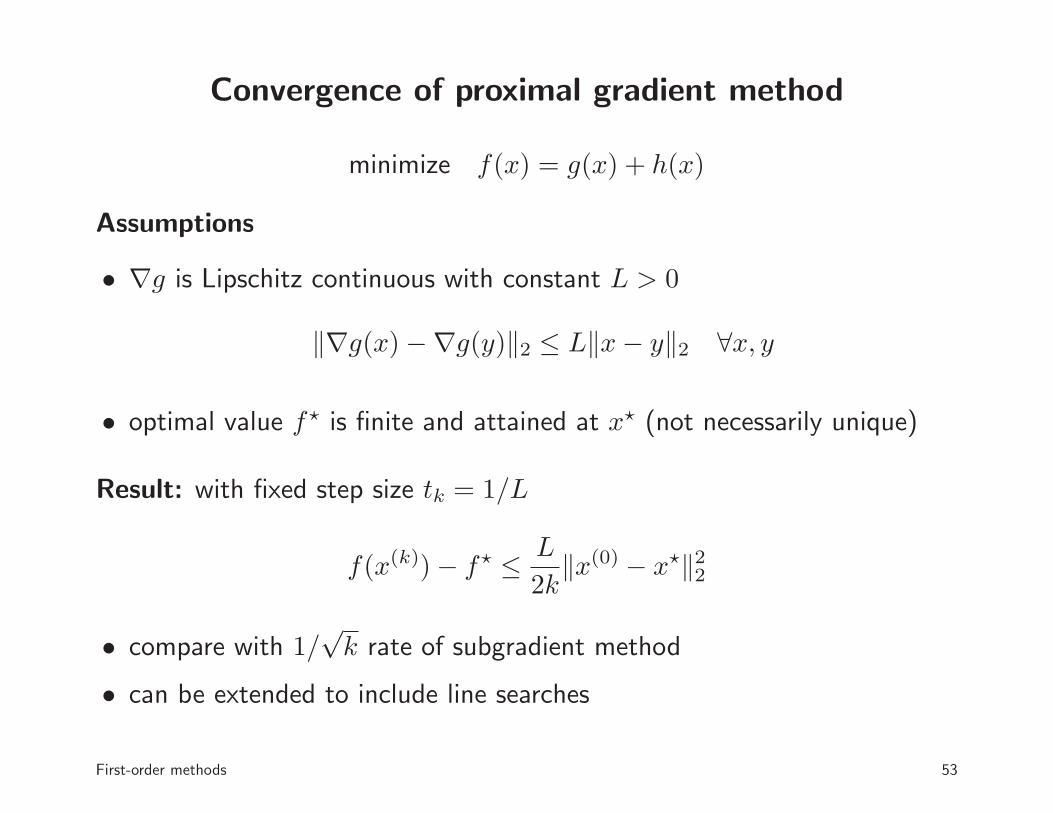
Convergence of proximal gradient method
minimize f(x) = g(x) + h(x)
Assumptions
• ∇g is Lipschitz continuous with constant L > 0
‖∇g(x)−∇g(y)‖2 ≤ L‖x− y‖2 ∀x, y
• optimal value f⋆ is finite and attained at x⋆ (not necessarily unique)
Result: with fixed step size tk = 1/L
f(x(k))− f⋆ ≤ L
2k‖x(0) − x⋆‖22
• compare with 1/√k rate of subgradient method
• can be extended to include line searches
First-order methods 53
Fast (proximal) gradient methods
• Nesterov (1983, 1988, 2005): three gradient projection methods with1/k2 convergence rate
• Beck & Teboulle (2008): FISTA, a proximal gradient version ofNesterov’s 1983 method
• Nesterov (2004 book), Tseng (2008): overview and unified analysis offast gradient methods
• several recent variations and extensions
This lecture: FISTA (Fast Iterative Shrinkage-Thresholding Algorithm)
First-order methods 54
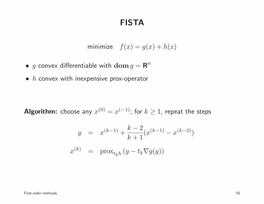
FISTA
minimize f(x) = g(x) + h(x)
• g convex differentiable with dom g = Rn
• h convex with inexpensive prox-operator
Algorithm: choose any x(0) = x(−1); for k ≥ 1, repeat the steps
y = x(k−1) +k − 2
k + 1(x(k−1) − x(k−2))
x(k) = proxtkh (y − tk∇g(y))
First-order methods 55
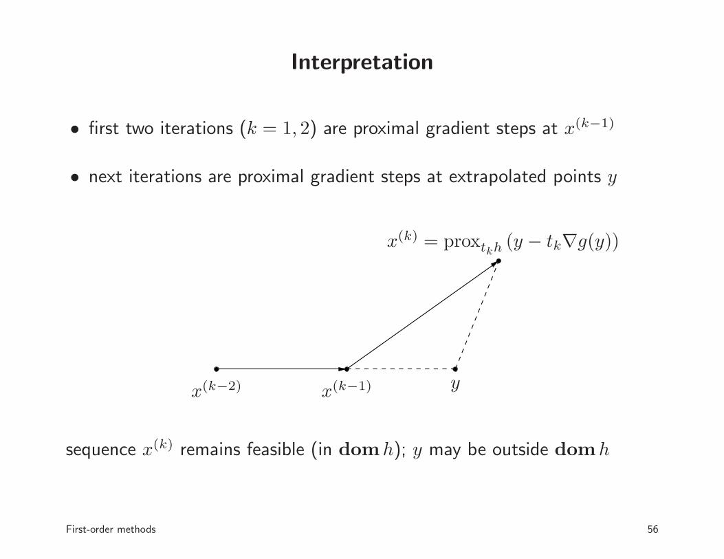
Interpretation
• first two iterations (k = 1, 2) are proximal gradient steps at x(k−1)
• next iterations are proximal gradient steps at extrapolated points y
x(k−2) x(k−1) y
x(k) = proxtkh (y − tk∇g(y))
sequence x(k) remains feasible (in domh); y may be outside domh
First-order methods 56
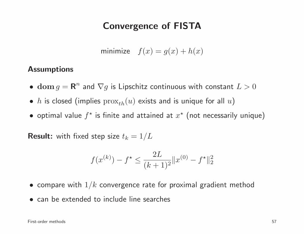
Convergence of FISTA
minimize f(x) = g(x) + h(x)
Assumptions
• dom g = Rn and ∇g is Lipschitz continuous with constant L > 0
• h is closed (implies proxth(u) exists and is unique for all u)
• optimal value f⋆ is finite and attained at x⋆ (not necessarily unique)
Result: with fixed step size tk = 1/L
f(x(k))− f⋆ ≤ 2L
(k + 1)2‖x(0) − f⋆‖22
• compare with 1/k convergence rate for proximal gradient method
• can be extended to include line searches
First-order methods 57
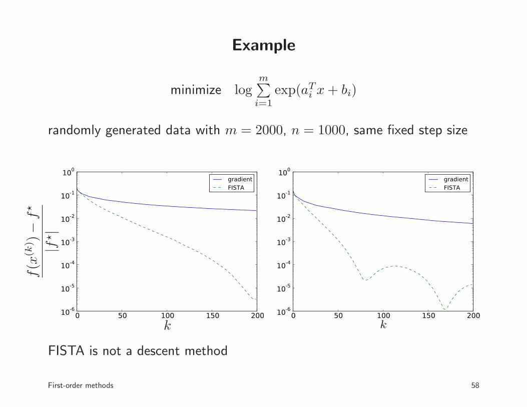
Example
minimize logm∑
i=1
exp(aTi x+ bi)
randomly generated data with m = 2000, n = 1000, same fixed step size
0 50 100 150 20010-6
10-5
10-4
10-3
10-2
10-1
100
gradientFISTA
k
f(x
(k) )−
f⋆
|f⋆|
0 50 100 150 20010-6
10-5
10-4
10-3
10-2
10-1
100
gradientFISTA
k
FISTA is not a descent method
First-order methods 58
Proximal point algorithm
to minimize h(x), apply fixed-point iteration to proxth
x+ = proxth(x)
• proximal gradient method with zero g
• implementable if inexact prox-evaluations are used
Convergence
• O(1/ǫ) iterations to reach h(x)− h(x⋆) ≤ ǫ (rate 1/k)
• O(1/√ǫ) iterations with accelerated (1/k2) algorithm (Guler 1992)
First-order methods 59
Smoothing interpretation
Moreau-Yosida regularization of h
h(t)(x) = infu
(
h(u) +1
2t‖u− x‖22
)
• convex, with full domain
• differentiable with 1/t-Lipschitz continuous gradient
∇h(t)(x) =1
t(x− proxth(x)) = proxh∗/t(x/t)
Proximal point algorithm (with constant t): gradient method for h(t)
x+ = proxth(x) = x− t∇h(t)(x)
First-order methods 60
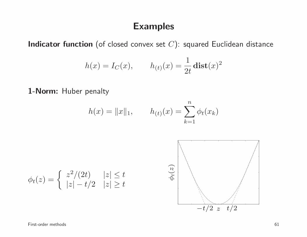
Examples
Indicator function (of closed convex set C): squared Euclidean distance
h(x) = IC(x), h(t)(x) =1
2tdist(x)2
1-Norm: Huber penalty
h(x) = ‖x‖1, h(t)(x) =
n∑
k=1
φt(xk)
φt(z) =
{z2/(2t) |z| ≤ t|z| − t/2 |z| ≥ t
t/2−t/2 z
φt(z)
First-order methods 61
Monotone operator
Monotone (set-valued) operator. F : Rn → Rn with
(y − y)T (x− x) ≥ 0 ∀x, x, y ∈ F (x), y ∈ F (x)
Examples
• subdifferential F (x) = ∂f(x) of closed convex function
• linear function F (x) = Bx with B +BT positive semidefinite
First-order methods 62
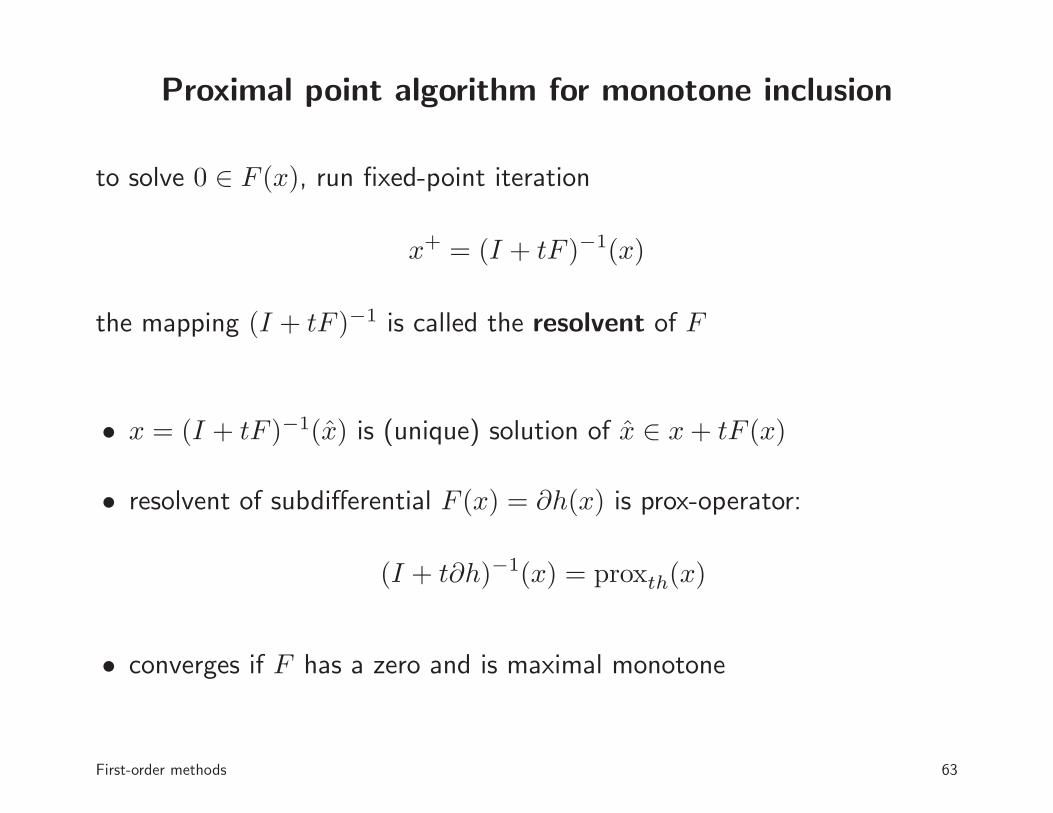
Proximal point algorithm for monotone inclusion
to solve 0 ∈ F (x), run fixed-point iteration
x+ = (I + tF )−1(x)
the mapping (I + tF )−1 is called the resolvent of F
• x = (I + tF )−1(x) is (unique) solution of x ∈ x+ tF (x)
• resolvent of subdifferential F (x) = ∂h(x) is prox-operator:
(I + t∂h)−1(x) = proxth(x)
• converges if F has a zero and is maximal monotone
First-order methods 63
Outline
• (proximal) gradient method
• splitting and alternating minimization methods
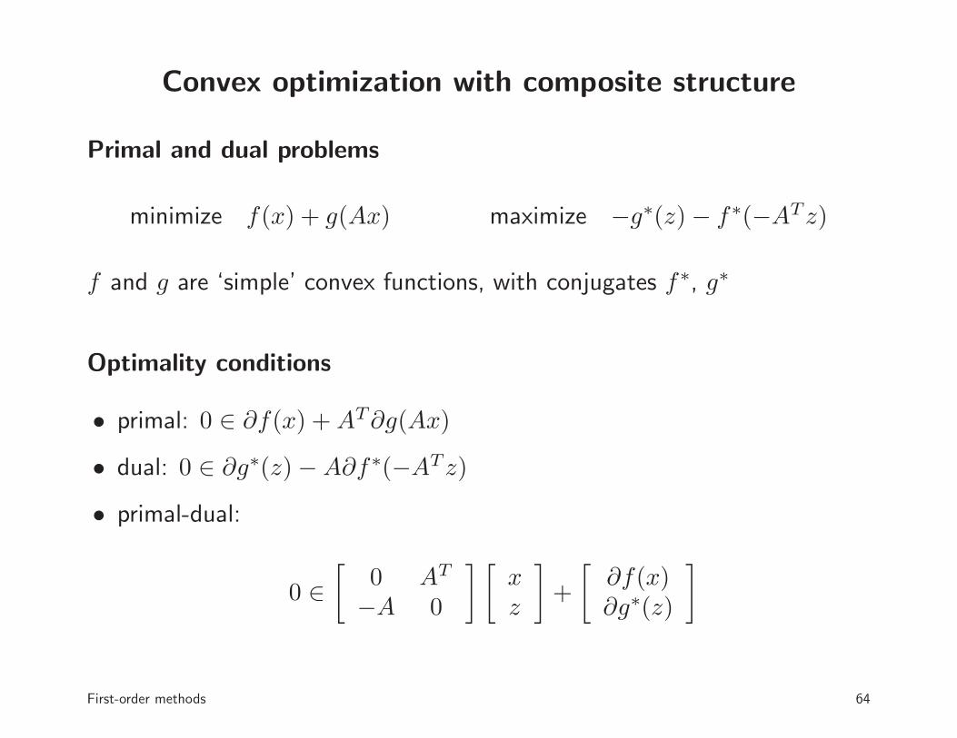
Convex optimization with composite structure
Primal and dual problems
minimize f(x) + g(Ax) maximize −g∗(z)− f∗(−ATz)
f and g are ‘simple’ convex functions, with conjugates f∗, g∗
Optimality conditions
• primal: 0 ∈ ∂f(x) +AT∂g(Ax)
• dual: 0 ∈ ∂g∗(z)−A∂f∗(−ATz)
• primal-dual:
0 ∈[
0 AT
−A 0
] [xz
]
+
[∂f(x)∂g∗(z)
]
First-order methods 64
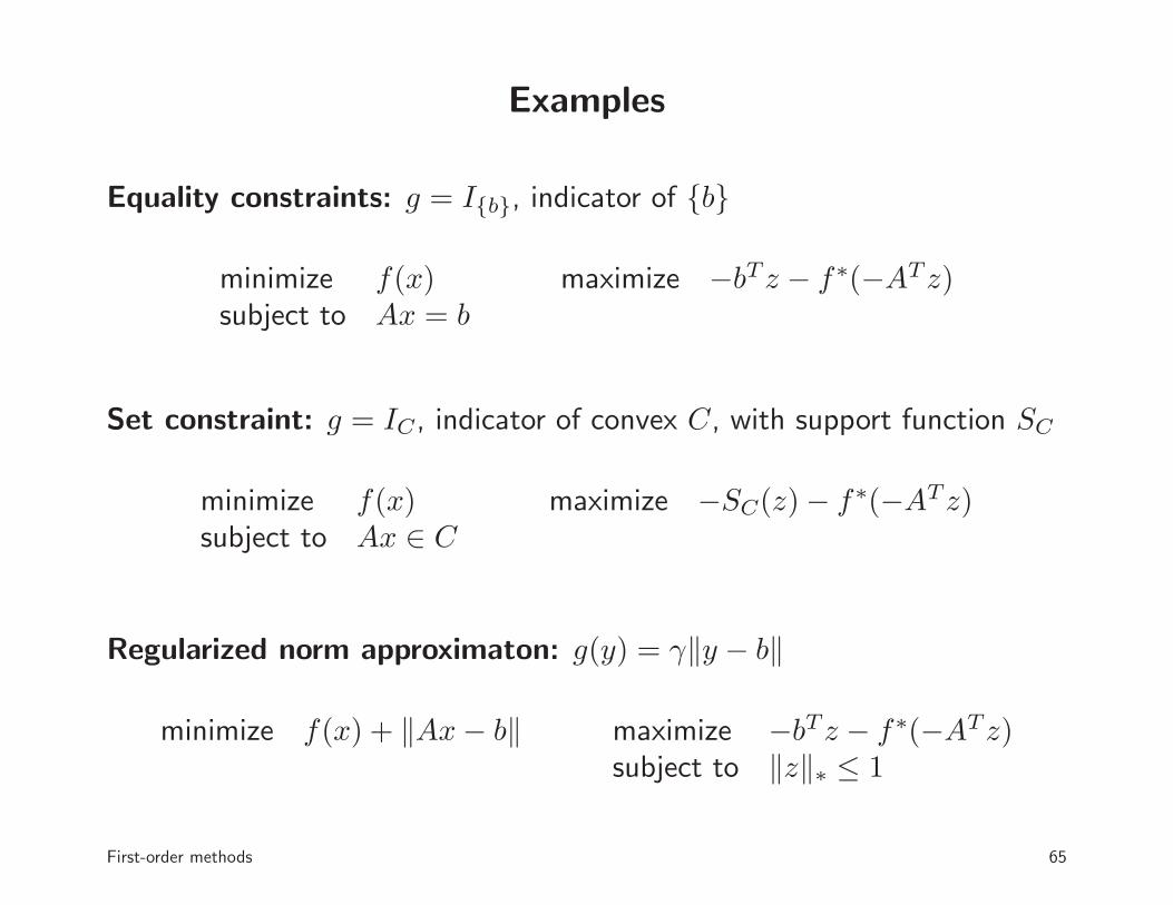
Examples
Equality constraints: g = I{b}, indicator of {b}
minimize f(x)subject to Ax = b
maximize −bTz − f∗(−ATz)
Set constraint: g = IC, indicator of convex C, with support function SC
minimize f(x)subject to Ax ∈ C
maximize −SC(z)− f∗(−ATz)
Regularized norm approximaton: g(y) = γ‖y − b‖
minimize f(x) + ‖Ax− b‖ maximize −bTz − f∗(−ATz)subject to ‖z‖∗ ≤ 1
First-order methods 65
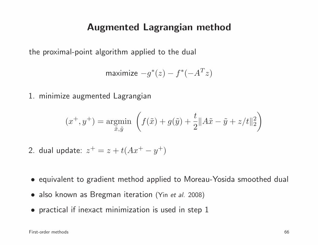
Augmented Lagrangian method
the proximal-point algorithm applied to the dual
maximize −g∗(z)− f∗(−ATz)
1. minimize augmented Lagrangian
(x+, y+) = argminx,y
(
f(x) + g(y) +t
2‖Ax− y + z/t‖22
)
2. dual update: z+ = z + t(Ax+ − y+)
• equivalent to gradient method applied to Moreau-Yosida smoothed dual
• also known as Bregman iteration (Yin et al. 2008)
• practical if inexact minimization is used in step 1
First-order methods 66
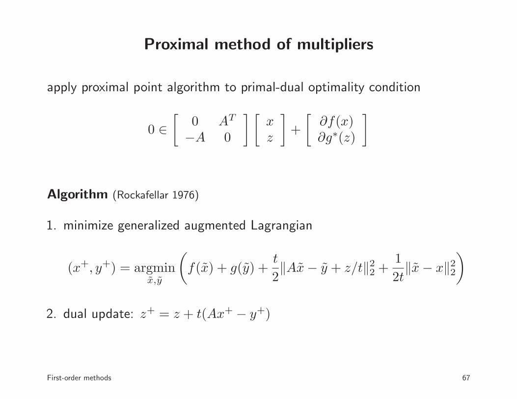
Proximal method of multipliers
apply proximal point algorithm to primal-dual optimality condition
0 ∈[
0 AT
−A 0
] [xz
]
+
[∂f(x)∂g∗(z)
]
Algorithm (Rockafellar 1976)
1. minimize generalized augmented Lagrangian
(x+, y+) = argminx,y
(
f(x) + g(y) +t
2‖Ax− y + z/t‖22 +
1
2t‖x− x‖22
)
2. dual update: z+ = z + t(Ax+ − y+)
First-order methods 67
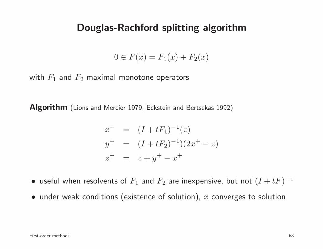
Douglas-Rachford splitting algorithm
0 ∈ F (x) = F1(x) + F2(x)
with F1 and F2 maximal monotone operators
Algorithm (Lions and Mercier 1979, Eckstein and Bertsekas 1992)
x+ = (I + tF1)−1(z)
y+ = (I + tF2)−1)(2x+ − z)
z+ = z + y+ − x+
• useful when resolvents of F1 and F2 are inexpensive, but not (I + tF )−1
• under weak conditions (existence of solution), x converges to solution
First-order methods 68
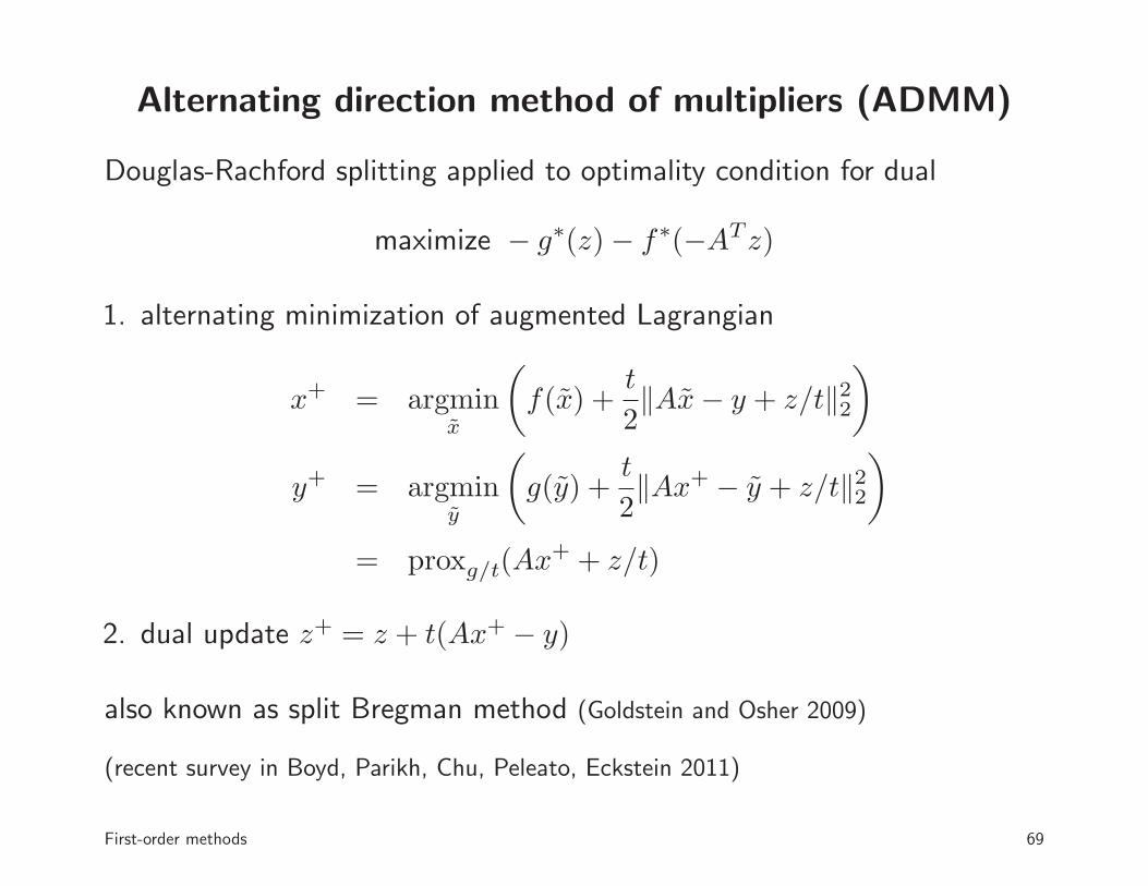
Alternating direction method of multipliers (ADMM)
Douglas-Rachford splitting applied to optimality condition for dual
maximize − g∗(z)− f∗(−ATz)
1. alternating minimization of augmented Lagrangian
x+ = argminx
(
f(x) +t
2‖Ax− y + z/t‖22
)
y+ = argminy
(
g(y) +t
2‖Ax+ − y + z/t‖22
)
= proxg/t(Ax+ + z/t)
2. dual update z+ = z + t(Ax+ − y)
also known as split Bregman method (Goldstein and Osher 2009)
(recent survey in Boyd, Parikh, Chu, Peleato, Eckstein 2011)
First-order methods 69
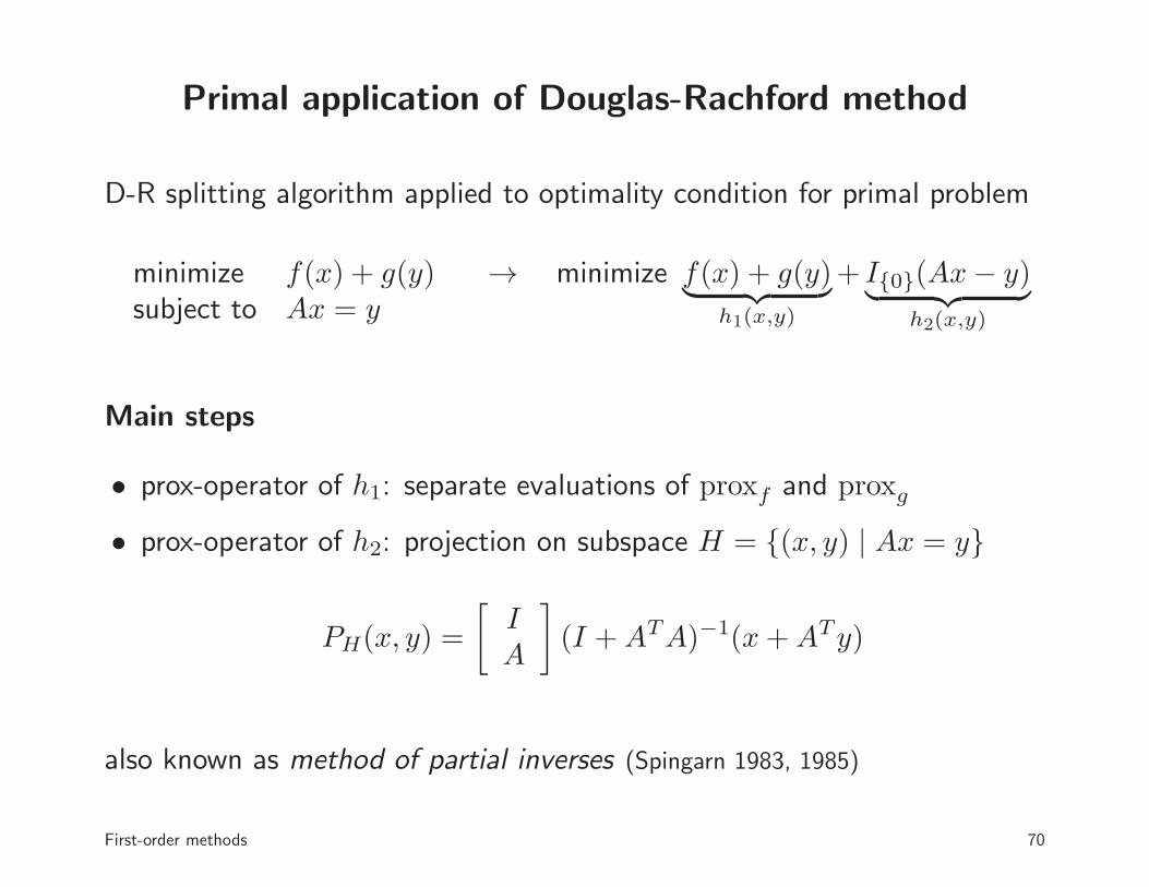
Primal application of Douglas-Rachford method
D-R splitting algorithm applied to optimality condition for primal problem
minimize f(x) + g(y)subject to Ax = y
→ minimize f(x) + g(y)︸ ︷︷ ︸
h1(x,y)
+ I{0}(Ax− y)︸ ︷︷ ︸
h2(x,y)
Main steps
• prox-operator of h1: separate evaluations of proxf and proxg
• prox-operator of h2: projection on subspace H = {(x, y) | Ax = y}
PH(x, y) =
[IA
]
(I +ATA)−1(x+ATy)
also known as method of partial inverses (Spingarn 1983, 1985)
First-order methods 70
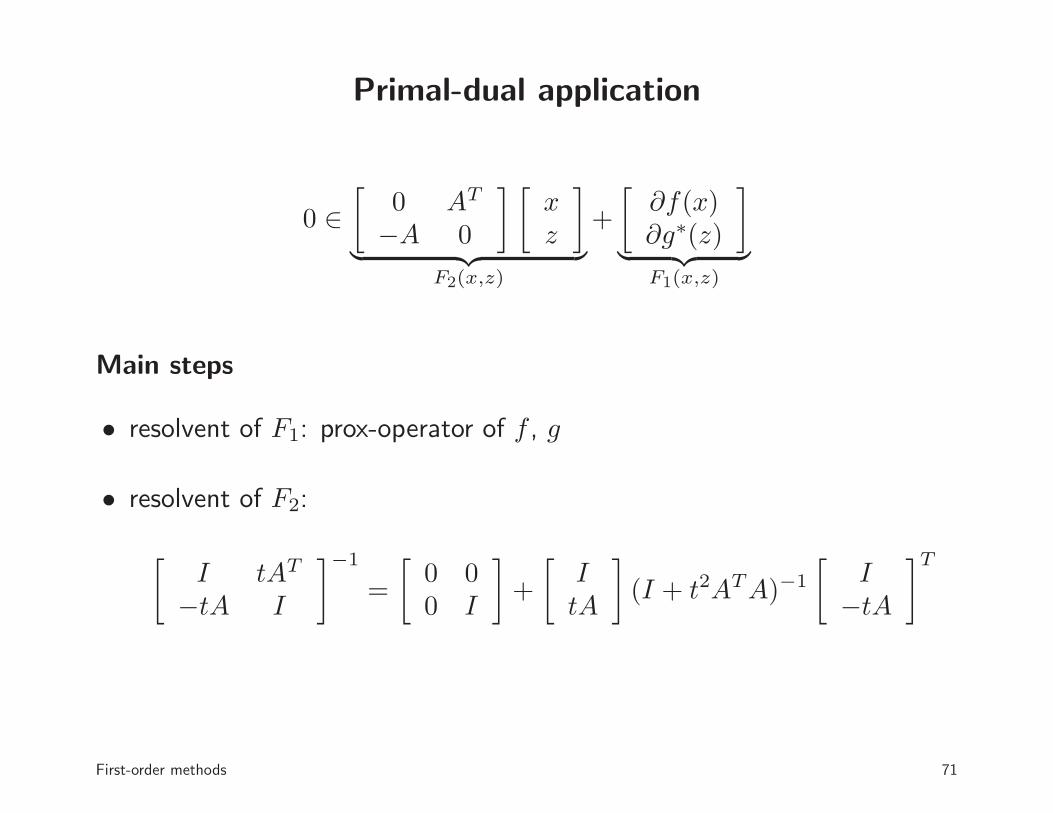
Primal-dual application
0 ∈[
0 AT
−A 0
] [xz
]
︸ ︷︷ ︸
F2(x,z)
+
[∂f(x)∂g∗(z)
]
︸ ︷︷ ︸
F1(x,z)
Main steps
• resolvent of F1: prox-operator of f , g
• resolvent of F2:
[I tAT
−tA I
]−1
=
[0 00 I
]
+
[ItA
]
(I + t2ATA)−1
[I
−tA
]T
First-order methods 71
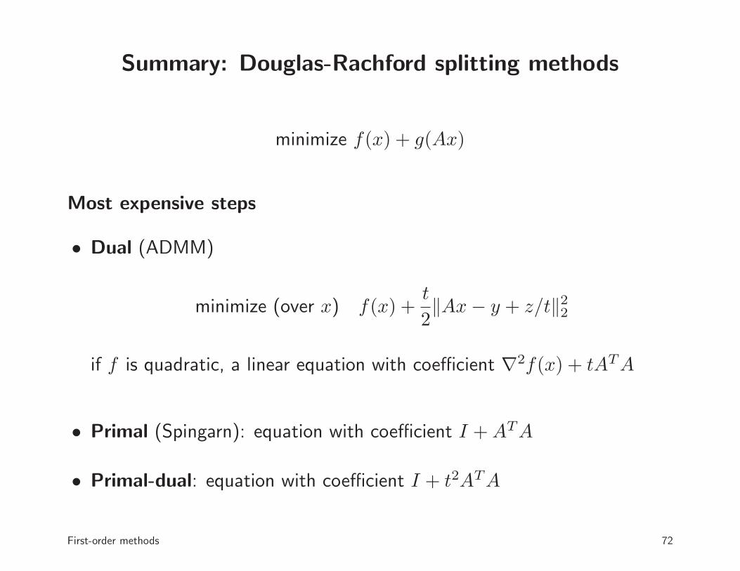
Summary: Douglas-Rachford splitting methods
minimize f(x) + g(Ax)
Most expensive steps
• Dual (ADMM)
minimize (over x) f(x) +t
2‖Ax− y + z/t‖22
if f is quadratic, a linear equation with coefficient ∇2f(x) + tATA
• Primal (Spingarn): equation with coefficient I +ATA
• Primal-dual: equation with coefficient I + t2ATA
First-order methods 72
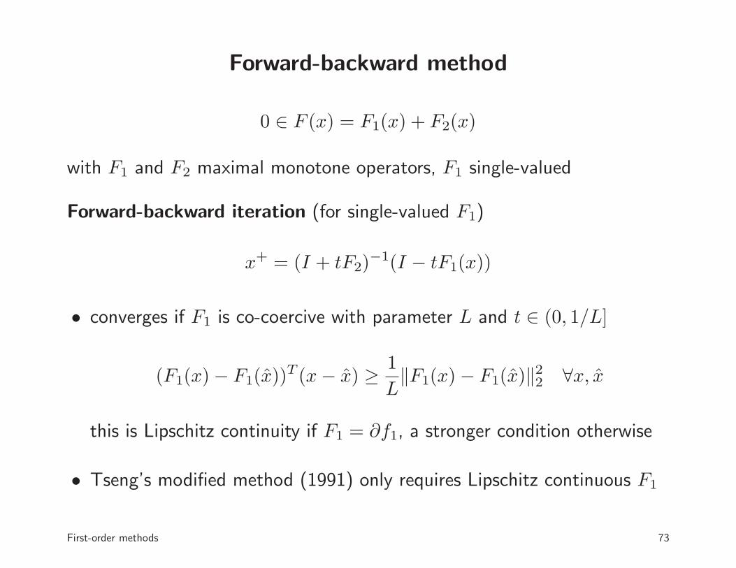
Forward-backward method
0 ∈ F (x) = F1(x) + F2(x)
with F1 and F2 maximal monotone operators, F1 single-valued
Forward-backward iteration (for single-valued F1)
x+ = (I + tF2)−1(I − tF1(x))
• converges if F1 is co-coercive with parameter L and t ∈ (0, 1/L]
(F1(x)− F1(x))T (x− x) ≥ 1
L‖F1(x)− F1(x)‖22 ∀x, x
this is Lipschitz continuity if F1 = ∂f1, a stronger condition otherwise
• Tseng’s modified method (1991) only requires Lipschitz continuous F1
First-order methods 73
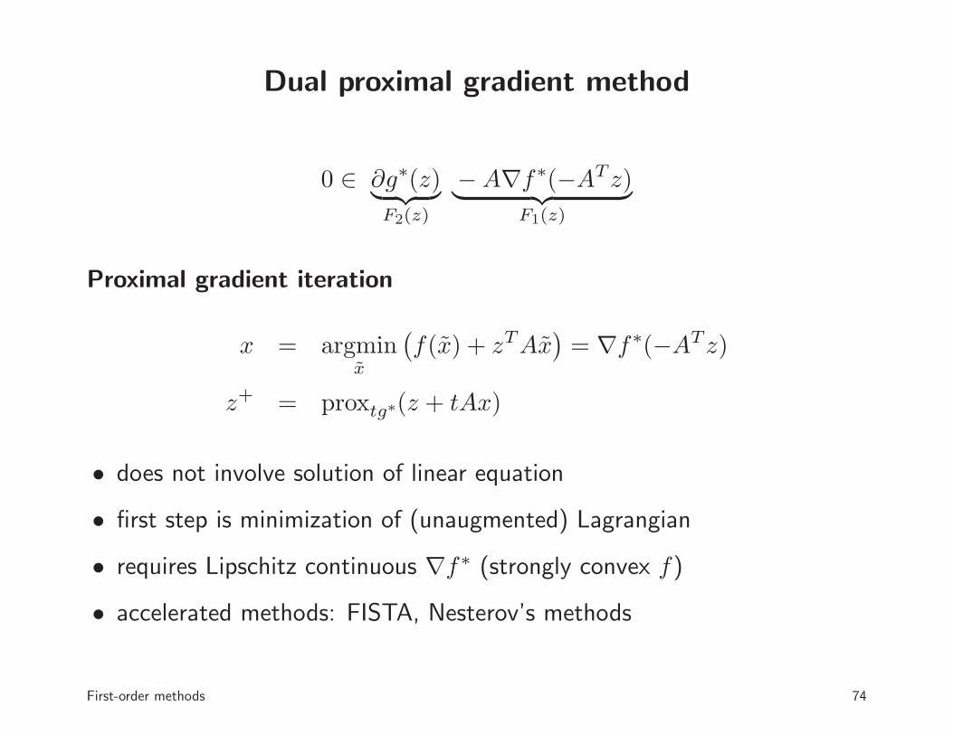
Dual proximal gradient method
0 ∈ ∂g∗(z)︸ ︷︷ ︸
F2(z)
−A∇f∗(−ATz)︸ ︷︷ ︸
F1(z)
Proximal gradient iteration
x = argminx
(f(x) + zTAx
)= ∇f∗(−ATz)
z+ = proxtg∗(z + tAx)
• does not involve solution of linear equation
• first step is minimization of (unaugmented) Lagrangian
• requires Lipschitz continuous ∇f∗ (strongly convex f)
• accelerated methods: FISTA, Nesterov’s methods
First-order methods 74
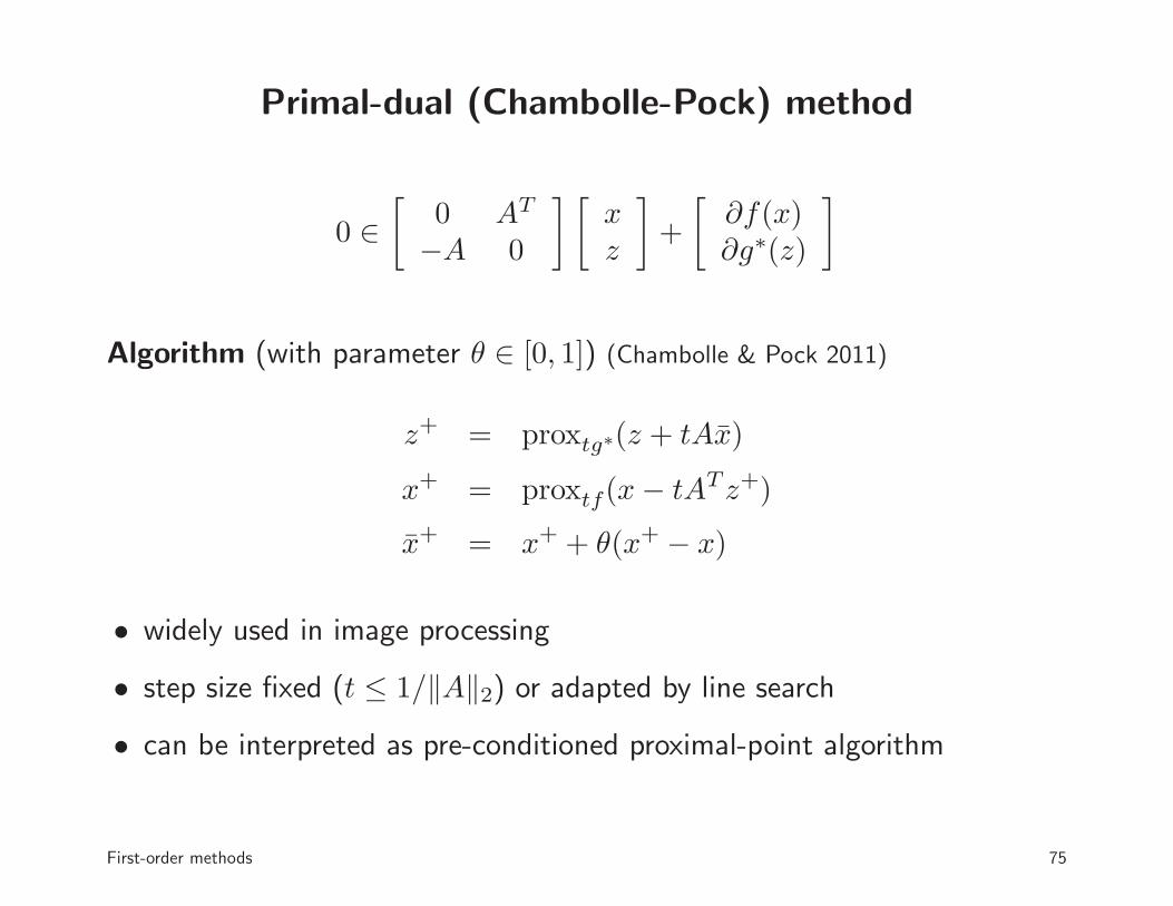
Primal-dual (Chambolle-Pock) method
0 ∈[
0 AT
−A 0
] [xz
]
+
[∂f(x)∂g∗(z)
]
Algorithm (with parameter θ ∈ [0, 1]) (Chambolle & Pock 2011)
z+ = proxtg∗(z + tAx)
x+ = proxtf(x− tATz+)
x+ = x+ + θ(x+ − x)
• widely used in image processing
• step size fixed (t ≤ 1/‖A‖2) or adapted by line search
• can be interpreted as pre-conditioned proximal-point algorithm
First-order methods 75
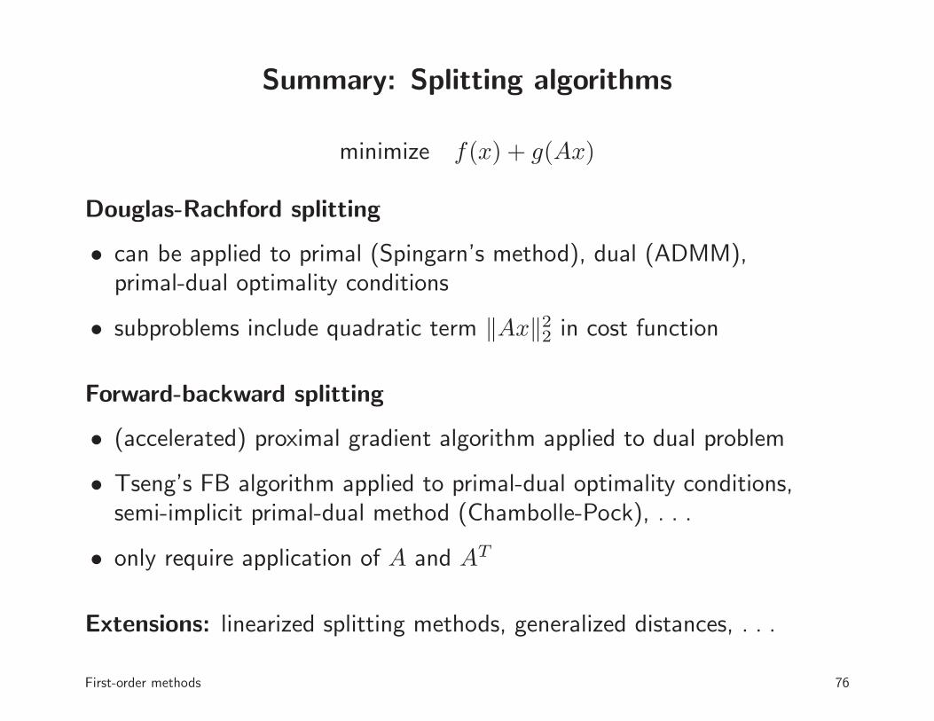
Summary: Splitting algorithms
minimize f(x) + g(Ax)
Douglas-Rachford splitting
• can be applied to primal (Spingarn’s method), dual (ADMM),primal-dual optimality conditions
• subproblems include quadratic term ‖Ax‖22 in cost function
Forward-backward splitting
• (accelerated) proximal gradient algorithm applied to dual problem
• Tseng’s FB algorithm applied to primal-dual optimality conditions,semi-implicit primal-dual method (Chambolle-Pock), . . .
• only require application of A and AT
Extensions: linearized splitting methods, generalized distances, . . .
First-order methods 76


![Domain Specific Languages [0.5ex] for Convex Optimization](https://static.fdocument.org/doc/165x107/61fb7d612e268c58cd5ec7a1/domain-specific-languages-05ex-for-convex-optimization.jpg)