Introduction to Complex Analysis

Michael Taylor

1

2

Contents

Chapter 1. Basic calculus in the complex domain

0. Complex numbers, power series, and exponentials1. Holomorphic functions, derivatives, and path integrals2. Holomorphic functions defined by power series3. Exponential and trigonometric functions: Euler’s formula4. Square roots, logs, and other inverse functionsI. π2 is irrational

Chapter 2. Going deeper – the Cauchy integral theorem and consequences

5. The Cauchy integral theorem and the Cauchy integral formula6. The maximum principle, Liouville’s theorem, and the fundamental theorem of al-

gebra7. Harmonic functions on planar regions8. Morera’s theorem, the Schwarz reflection principle, and Goursat’s theorem9. Infinite products

10. Uniqueness and analytic continuation11. Singularities12. Laurent seriesC. Green’s theoremF. The fundamental theorem of algebra (elementary proof)L. Absolutely convergent series

Chapter 3. Fourier analysis and complex function theory

13. Fourier series and the Poisson integral14. Fourier transforms15. Laplace transforms and Mellin transformsH. Inner product spacesN. The matrix exponentialG. The Weierstrass and Runge approximation theorems

Chapter 4. Residue calculus, the argument principle, and two very specialfunctions

16. Residue calculus17. The argument principle18. The Gamma function19. The Riemann zeta function and the prime number theoremJ. Euler’s constantS. Hadamard’s factorization theorem

3

Chapter 5. Conformal maps and geometrical aspects of complex function the-ory

20. Conformal maps21. Normal families22. The Riemann sphere (and other Riemann surfaces)23. The Riemann mapping theorem24. Boundary behavior of conformal maps25. Covering maps26. The disk covers C \ 0, 127. Montel’s theorem28. Picard’s theorems29. Harmonic functions IID. Surfaces and metric tensorsE. Poincare metrics

Chapter 6. Elliptic functions and elliptic integrals

30. Periodic and doubly periodic functions - infinite series representations31. The Weierstrass ℘ in elliptic function theory32. Theta functions and ℘33. Elliptic integrals34. The Riemann surface of

√q(ζ)

K. Rapid evaluation of the Weierstrass ℘-function

Chapter 7. Complex analysis and differential equations

35. Bessel functions36. Differential equations on a complex domainO. From wave equations to Bessel and Legendre equations

Appendices

A. Metric spaces, convergence, and compactnessB. Derivatives and diffeomorphismsP. The Laplace asymptotic method and Stirling’s formulaM. The Stieltjes integralR. Abelian theorems and Tauberian theoremsQ. Cubics, quartics, and quintics

4

Preface

This text is designed for a first course in complex analysis, for beginning graduate stu-dents, or well prepared undergraduates, whose background includes multivariable calculus,linear algebra, and advanced calculus. In this course the student will learn that all the basicfunctions that arise in calculus, first derived as functions of a real variable, such as powersand fractional powers, exponentials and logs, trigonometric functions and their inverses,and also many new functions that the student will meet, are naturally defined for complexarguments. Furthermore, this expanded setting reveals a much richer understanding ofsuch functions.

Care is taken to introduce these basic functions first in real settings. In the openingsection on complex power series and exponentials, in Chapter 1, the exponential functionis first introduced for real values of its argument, as the solution to a differential equation.This is used to derive its power series, and from there extend it to complex argument.Similarly sin t and cos t are first given geometrical definitions, for real angles, and theEuler identity is established based on the geometrical fact that eit is a unit-speed curve onthe unit circle, for real t. Then one sees how to define sin z and cos z for complex z.

The central objects in complex analysis are functions that are complex-differentiable(i.e., holomorphic). One goal in the early part of the text is to establish an equivalencebetween being holomorphic and having a convergent power series expansion. Half of thisequivalence, namely the holomorphy of convergent power series, is established in Chapter1.

Chapter 2 starts with two major theoretical results, the Cauchy integral theorem, andits corollary, the Cauchy integral formula. These theorems have a major impact on theentire rest of the text, including the demonstration that if a function f(z) is holomorphicon a disk, then it is given by a convergent power series on that disk. A useful variant ofsuch power series is the Laurent series, for a function holomorphic on an annulus.

The text segues from Laurent series to Fourier series, in Chapter 3, and from there to theFourier transform and the Laplace transform. These three topics have many applications inanalysis, such as constructing harmonic functions, and providing other tools for differentialequations. The Laplace transform of a function has the important property of beingholomorphic on a half space. It is convenient to have a treatment of the Laplace transformafter the Fourier transform, since the Fourier inversion formula serves to motivate andprovide a proof of the Laplace inversion formula.

Results on these transforms illuminate the material in Chapter 4. For example, thesetransforms are a major source of important definite integrals that one cannot evaluate byelementary means, but that are amenable to analysis by residue calculus, a key applicationof the Cauchy integral theorem. Chapter 4 starts with this, and proceeds to the study oftwo important special functions, the Gamma function and the Riemann zeta function.

The Gamma function, which is the first “higher” transcendental function, is essentiallya Laplace transform. The Riemann zeta function is a basic object of analytic number

5

theory, arising in the study of prime numbers. One sees in Chapter 4 roles of Fourieranalysis, residue calculus, and the Gamma function in the study of the zeta function. Forexample, a relation between Fourier series and the Fourier transform, known as the Poissonsummation formula, plays an important role in its study.

In Chapter 5, the text takes a geometrical turn, viewing holomorphic functions asconformal maps. This notion is pursued not only for maps between planar domains,but also for maps to surfaces in R3. The standard case is the unit sphere S2, and theassociated stereographic projection. The text also considers other surfaces. It constructsconformal maps from planar domains to general surfaces of revolution, deriving for the mapa first-order differential equation, nonlinear but separable. These surfaces are discussed

as examples of Riemann surfaces. The Riemann sphere C = C ∪ ∞ is also discussed asa Riemann surface, conformally equivalent to S2. One sees the group of linear fractional

transformations as a group of conformal automorphisms of C, and certain subgroups asgroups of conformal automorphisms of the unit disk and of the upper half plane.

We also bring in the notion of normal families, to prove the Riemann mapping theorem.Application of this theorem to a special domain, together with a reflection argument, showsthat there is a holomorphic covering of C\0, 1 by the unit disk. This leads to key resultsof Picard and Montel, and applications to the behavior of iterations of holomorphic maps

R : C → C, and the Julia sets that arise.

The treatment of Riemann surfaces includes some differential geometric material. Inan appendix to Chapter 5, we introduce the concept of a metric tensor, and show how itis associated to a surface in Euclidean space, and how the metric tensor behaves undersmooth mappings, and in particular how this behavior characterizes conformal mappings.We discuss the notion of metric tensors beyond the setting of metrics induced on surfacesin Euclidean space. In particular, we introduce a special metric on the unit disk, calledthe Poincare metric, which has the property of being invariant under all conformal auto-morphisms of the disk. We show how the geometry of the Poincare metric leads to anotherproof of Picard’s theorem, and also provides a different perspective on the proof of theRiemann mapping theorem.

The text next examines elliptic functions, in Chapter 6. These are doubly periodicfunctions on C, holomorphic except at poles (that is, meromorphic). Such a functioncan be regarded as a meromorphic function on the torus TΛ = C/Λ, where Λ ⊂ C is alattice. A prime example is the Weierstrass function ℘Λ(z), defined by a double series.Analysis shows that ℘′

Λ(z)2 is a cubic polynomial in ℘Λ(z), so the Weierstrass function

inverts an elliptic integral. Elliptic integrals arise in many situations in geometry andmechanics, including arclengths of ellipses and pendulum problems, to mention two basiccases. The analysis of general elliptic integrals leads to the problem of finding the latticewhose associated elliptic functions are related to these integrals. This is the Abel inversionproblem. Section 34 of the text tackles this problem by constructing the Riemann surfaceassociated to

√p(z), where p(z) is a cubic or quartic polynomial.

Early in this text, the exponential function was defined by a differential equation andgiven a power series solution, and these two characterizations were used to develop itsproperties. Coming full circle, we devote Chapter 7 to other classes of differential equations

6

and their solutions. We first study a special class of functions known as Bessel functions,characterized as solutions to Bessel equations. Part of the central importance of thesefunctions arises from their role in producing solutions to partial differential equations inseveral variables, as explained in an appendix. The Bessel functions for real values oftheir arguments arise as solutions to wave equations, and for imaginary values of theirarguments they arise as solutions to diffusion equations. Thus it is very useful that theycan be understood as holomorphic functions of a complex variable. Next, Chapter 7 dealswith more general differential equations on a complex domain. Results include constructingsolutions as convergent power series and the analytic continuation of such solutions to largerdomains. General results here are used to put the Bessel equations in a larger context. Thisincludes a study of equations with “regular singular points.” Other classes of equationswith regular singular points are presented, particularly hypergeometric equations.

The text ends with a short collection of appendices. Some of these survey backgroundmaterial that the reader might have seen in an advanced calculus course, including materialon convergence and compactness, and differential calculus of several variables. Othersdevelop tools that prove useful in the text, the Laplace asymptotic method, the Stieltjesintegral, and results on Abelian and Tauberian theorems. The last appendix shows how tosolve cubic and quartic equations via radicals, and introduces a special function, called theBring radical, to treat quintic equations. (In §36 the Bring radical is shown to be given interms of a generalized hypergeometric function.)

As indicated in the discussion above, while the first goal of this text is to present thebeautiful theory of functions of a complex variable, we have the further objective of placingthis study within a broader mathematical framework. Examples of how this text differsfrom many others in the area include the following.

1) A greater emphasis on Fourier analysis, both as an application of basic results in complexanalysis and as a tool of more general applicability in analysis. We see the use of Fourierseries in the study of harmonic functions. We see the influence of the Fourier transformon the study of the Laplace transform, and then the Laplace transform as a tool in thestudy of differential equations.

2) The use of geometrical techniques in complex analysis. This clarifies the study of con-formal maps, extends the usual study to more general surfaces, and shows how geometricalconcepts are effective in classical problems, from the Riemann mapping theorem to Picard’stheorem. An appendix discusses applications of the Poincare metric on the disk.

3) Connections with differential equations. The use of techniques of complex analysis tostudy differential equations is a strong point of this text. This important area is frequentlyneglected in complex analysis texts, and the treatments one sees in many differential equa-tions texts are often confined to solutions for real variables, and may furthermore lack acomplete analysis of crucial convergence issues. Material here also provides a more detailedstudy than one usually sees of significant examples, such as Bessel functions.

7

4) Special functions. In addition to material on the gamma function and the Riemann zetafunction, the text has a detailed study of elliptic functions and Bessel functions, and alsomaterial on Airy functions, Legendre functions, and hypergeometric functions.

We follow this introduction with a record of some standard notation that will be usedthroughout this text.

AcknowledgmentThanks to Shrawan Kumar for testing this text in his Complex Analysis course, for pointingout corrections, and for other valuable advice.

8

Some Basic Notation

R is the set of real numbers.

C is the set of complex numbers.

Z is the set of integers.

Z+ is the set of integers ≥ 0.

N is the set of integers ≥ 1 (the “natural numbers”).

x ∈ R means x is an element of R, i.e., x is a real number.

(a, b) denotes the set of x ∈ R such that a < x < b.

[a, b] denotes the set of x ∈ R such that a ≤ x ≤ b.

x ∈ R : a ≤ x ≤ b denotes the set of x in R such that a ≤ x ≤ b.

[a, b) = x ∈ R : a ≤ x < b and (a, b] = x ∈ R : a < x ≤ b.

z = x− iy if z = x+ iy ∈ C, x, y ∈ R.

Ω denotes the closure of the set Ω.

f : A→ B denotes that the function f takes points in the set A to pointsin B. One also says f maps A to B.

x→ x0 means the variable x tends to the limit x0.

f(x) = O(x) means f(x)/x is bounded. Similarly g(ε) = O(εk) meansg(ε)/εk is bounded.

f(x) = o(x) as x→ 0 (resp., x→ ∞) means f(x)/x→ 0 as x tends to thespecified limit.

S = supn

|an| means S is the smallest real number that satisfies S ≥ |an| for all n.If there is no such real number then we take S = +∞.

lim supk→∞

|ak| = limn→∞

(supk≥n

|ak|).

9

Chapter 1. Basic calculus in the complex domain

This first chapter introduces the complex numbers and begins to develop results on thebasic elementary functions of calculus, first defined for real arguments, and then extendedto functions of a complex variable.

An introductory §0 defines the algebraic operations on complex numbers, say z = x+ iyand w = u+ iv, discusses the magnitude |z| of z, defines convergence of infinite sequencesand series, and derives some basic facts about power series

(1.0.1) f(z) =

∞∑k=0

akzk,

such as the fact that if this converges for z = z0, then it converges absolutely for |z| <R = |z0|, to a continuous function. It is also shown that, for z = t real,

(1.0.2) f ′(t) =∑k≥1

kaktk−1, for −R < t < R.

Here we allow ak ∈ C. As an application, we consider the differential equation

(1.0.3)dx

dt= x, x(0) = 1,

and deduce from (1.0.2) that a solution is given by x(t) =∑k≥0 t

k/k!. Having this, wedefine the exponential function

(1.0.4) ez =

∞∑k=0

1

k!zk,

and use these observations to deduce that, whenever a ∈ C,

(1.0.5)d

dteat = aeat.

We use this differential equation to derive further properties of the exponential function.While §0 develops calculus for complex valued functions of a real variable, §1 introduces

calculus for complex valued functions of a complex variable. We define the notion of com-plex differentiability. Given an open set Ω ⊂ C, we say a function f : Ω → C is holomorphicon Ω provided it is complex differentiable, with derivative f ′(z), and f ′ is continuous on Ω.Writing f(z) = u(z) + iv(z), we discuss the Cauchy-Riemann equations for u and v. Wealso introduce the path integral and provide some versions of the fundamental theorem ofcalculus in the complex setting. (More definitive results will be given in Chapter 2.)

10

Typically the functions we study are defined on a subset Ω ⊂ C that is open. That is,if z0 ∈ Ω, there exists ε > 0 such that z ∈ Ω whenever |z − z0| < ε. Other terms we usefor a nonempty open set are “domain” and “region.” These terms are used synonymouslyin this text.

In §2 we return to convergent power series and show they produce holomorphic functions.We extend results of §0 from functions of a real variable to functions of a complex variable.Section 3 returns to the exponential function ez, defined above. We extend (1.0.5) to

(1.0.6)d

dzeaz = aeaz.

We show that t 7→ et maps R one-to-one and onto (0,∞), and define the logarithm on(0,∞), as its inverse:

(1.0.7) x = et ⇐⇒ t = log x.

We also examine the behavior of γ(t) = eit, for t ∈ R, showing that this is a unit-speedcurve tracing out the unit circle. From this we deduce Euler’s formula,

(1.0.8) eit = cos t+ i sin t.

This leads to a direct, self-contained treatment of the trigonometric functions.In §4 we discuss inverses to holomorphic functions. In particular, we extend the loga-

rithm from (0,∞) to C \ (−∞, 0], as a holomorphic function. We define fractional powers

(1.0.9) za = ea log z, a ∈ C, z ∈ C \ (−∞, 0],

and investigate their basic properties. We also discuss inverse trigonometric functions inthe complex plane.

The number π arises in §3 as half the length of the unit circle, or equivalently thesmallest positive number satisfying

(1.0.10) eπi = −1.

This is possibly the most intriguing number in mathematics. It will appear many timesover the course of this text. One of our goals will be to obtain accurate numerical approx-imations to π. In another vein, in Appendix I we show that π2 is irrational.

11

0. Complex numbers, power series, and exponentials

A complex number has the form

(0.1) z = x+ iy,

where x and y are real numbers. These numbers make up the complex plane, which isjust the xy-plane with the real line forming the horizontal axis and the real multiples of iforming the vertical axis. See Figure 0.1. We write

(0.2) x = Re z, y = Im z.

We write x, y ∈ R and z ∈ C. We identify x ∈ R with x+ i0 ∈ C. If also w = u+ iv withu, v ∈ R, we have addition and multiplication, given by

(0.3)z + w = (x+ u) + i(y + v),

zw = (xu− yv) + i(xv + yu),

the latter rule containing the identity

(0.4) i2 = −1.

One readily verifies the commutative laws

(0.5) z + w = w + z, zw = wz,

the associative laws (with also c ∈ C)

(0.6) z + (w + c) = (z + w) + c, z(wc) = (zw)c,

and the distributive law

(0.7) c(z + w) = cz + cw,

as following from their counterparts for real numbers. If c = 0, we can perform divisionby c,

z

c= w ⇐⇒ z = wc.

See (0.13) for a neat formula.For z = x+iy, we define |z| to be the distance of z from the origin 0, via the Pythagorean

theorem:

(0.8) |z| =√x2 + y2.

12

Note that

(0.9) |z|2 = z z, where z = x− iy,

is called the complex conjugate of z. One readily checks that

(0.10) z + z = 2 Re z, z − z = 2i Im z,

and

(0.11) z + w = z + w, zw = z w.

Hence |zw|2 = zwz w = |z|2|w|2, so

(0.12) |zw| = |z| · |w|.

We also have, for c = 0,

(0.13)z

c=

1

|c|2zc.

The following result is known as the triangle inequality, as Figure 0.2 suggests.

Proposition 0.1. Given z, w ∈ C,

(0.14) |z + w| ≤ |z|+ |w|.

Proof. We compare the squares of the two sides:

(0.15)

|z + w|2 = (z + w)(z + w)

= zz + ww + zw + wz

= |z|2 + |w|2 + 2 Re(zw),

while

(0.16)(|z|+ |w|)2 = |z|2 + |w|2 + 2|z| · |w|

= |z|2 + |w|2 + 2|zw|.

Thus (0.14) follows from the inequality Re(zw) ≤ |zw|, which in turn is immediate fromthe definition (0.8). (For any ζ ∈ C, Re ζ ≤ |ζ|.)

We can define convergence of a sequence (zn) in C as follows. We say

(0.17) zn → z if and only if |zn − z| → 0,

13

the latter notion involving convergence of a sequence of real numbers. Clearly if zn =xn + iyn and z = x+ iy, with xn, yn, x, y ∈ R, then

(0.18) zn → z if and only if xn → x and yn → y.

One readily verifies that

(0.19) zn → z, wn → w =⇒ zn + wn → z + w and znwn → zw,

as a consequence of their counterparts for sequences of real numbers.A related notion is that a sequence (zn) in C is Cauchy if and only if

(0.19A) |zn − zm| −→ 0 as m,n→ ∞.

As in (0.18), this holds if and only if (xn) and (yn) are Cauchy in R. The following is animportant fact.

(0.19B) Each Cauchy sequence in C converges.

This follows from the fact that

(0.19C) each Cauchy sequence in R converges.

A detailed presentation of the field R of real numbers, including a proof of (0.19C), is givenin Chapter 1 of [T0].

We can define the notion of convergence of an infinite series

(0.20)

∞∑k=0

zk

as follows. For each n ∈ Z+, set

(0.21) sn =

n∑k=0

zk.

Then (0.20) converges if and only if the sequence (sn) converges:

(0.22) sn → w =⇒∞∑k=0

zk = w.

Note that

(0.23)

|sn+m − sn| =∣∣∣ n+m∑k=n+1

zk

∣∣∣≤

n+m∑k=n+1

|zk|.

Using this, we can establish the following.

14

Lemma 0.1A. Assume that

(0.24)∞∑k=0

|zk| <∞,

i.e., there exists A <∞ such that

(0.24A)

N∑k=0

|zk| ≤ A, ∀N.

Then the sequence (sn) given by (0.21) is Cauchy, hence the series (0.20) is convergent.

Proof. If (sn) is not Cauchy, there exist a > 0, nν ∞, and mν > 0 such that

|snν+mν− snν

| ≥ a.

Passing to a subsequence, one can assume that nν+1 > nν +mν . Then (0.23) implies

mν+nν∑k=0

|zk| ≥ νa, ∀ ν,

contradicting (0.24A).

If (0.24) holds, we say the series (0.20) is absolutely convergent.An important class of infinite series is the class of power series

(0.25)∞∑k=0

akzk,

with ak ∈ C. Note that if z1 = 0 and (0.25) converges for z = z1, then there exists C <∞such that

(0.25A) |akzk1 | ≤ C, ∀ k.

Hence, if |z| ≤ r|z1|, r < 1, we have

(0.26)∞∑k=0

|akzk| ≤ C∞∑k=0

rk =C

1− r<∞,

the last identity being the classical geometric series computation. See Exercise 3 below.This yields the following.

15

Proposition 0.2. If (0.25) converges for some z1 = 0, then either this series is absolutelyconvergent for all z ∈ C, or there is some R ∈ (0,∞) such that the series is absolutelyconvergent for |z| < R and divergent for |z| > R.

We call R the radius of convergence of (0.25). In case of convergence for all z, we saythe radius of convergence is infinite. If R > 0 and (0.25) converges for |z| < R, it definesa function

(0.27) f(z) =

∞∑k=0

akzk, z ∈ DR,

on the disk of radius R centered at the origin,

(0.28) DR = z ∈ C : |z| < R.

Proposition 0.3. If the series (0.27) converges in DR, then f is continuous on DR, i.e.,given zn, z ∈ DR,

(0.29) zn → z =⇒ f(zn) → f(z).

Proof. For each z ∈ DR, there exists S < R such that z ∈ DS , so it suffices to show thatf is continuous on DS whenever 0 < S < R. Pick T such that S < T < R. We know thatthere exists C <∞ such that |akT k| ≤ C for all k. Hence

(0.30) z ∈ DS =⇒ |akzk| ≤ C(ST

)k.

For each N , write

(0.31)

f(z) = SN (z) +RN (z),

SN (z) =N∑k=0

akzk, RN (z) =

∞∑k=N+1

akzk.

Each SN (z) is a polynomial in z, and it follows readily from (0.19) that SN is continuous.Meanwhile,

(0.32) z ∈ DS ⇒ |RN (z)| ≤∞∑

k=N+1

|akzk| ≤ C

∞∑k=N+1

(ST

)k= CεN ,

and εN → 0 as N → ∞, independently of z ∈ DS . Continuity of f on DS follows, as aconsequence of the next lemma.

16

Lemma 0.3A. Let SN : DS → C be continuous functions. Assume f : DS → C andSN → f uniformly on DS, i.e.,

(0.32A) |SN (z)− f(z)| ≤ δN , ∀ z ∈ DS , δN → 0, as N → ∞.

Then f is continuous on DS.

Proof. Let zn → z in DS . We need to show that, given ε > 0, there existsM =M(ε) <∞such that

|f(z)− f(zn)| ≤ ε, ∀n ≥M.

To get this, pick N such that (0.32A) holds with δN = ε/3. Now use continuity of SN , todeduce that there exists M such that

|SN (z)− SN (zn)| ≤ε

3, ∀n ≥M.

It follows that, for n ≥M ,

|f(z)− f(zn)| ≤ |f(z)− SN (z)|+ |SN (z)− SN (zn)|+ |SN (zn)− f(zn)|

≤ ε

3+ε

3+ε

3,

as desired.

Remark. The estimate (0.32) says the series (0.27) converges uniformly on DS , for eachS < R.

A major consequence of material developed in §§1–5 will be that a function on DR

is given by a convergent power series (0.27) if and only if f has the property of beingholomorphic on DR (a property that is defined in §1). We will be doing differential andintegral calculus on such functions. In this preliminary section, we restrict z to be real,and do some calculus, starting with the following.

Proposition 0.4. Assume ak ∈ C and

(0.33) f(t) =

∞∑k=0

aktk

converges for real t satisfying |t| < R. Then f is differentiable on the interval −R < t < R,and

(0.34) f ′(t) =∞∑k=1

kaktk−1,

the latter series being absolutely convergent for |t| < R.

17

We first check absolute convergence of the series (0.34). Let S < T < R. Convergenceof (0.33) implies there exists C <∞ such that

(0.35) |ak|T k ≤ C, ∀ k.

Hence, if |t| ≤ S,

(0.35A) |kaktk−1| ≤ C

Sk(ST

)k.

The absolute convergence of

(0.36)∞∑k=0

krk, for |r| < 1,

follows from the ratio test. (See Exercises 4–5 below.) Hence

(0.37) g(t) =

∞∑k=1

kaktk−1

is continuous on (−R,R). To show that f ′(t) = g(t), by the fundamental theorem ofcalculus, it is equivalent to show

(0.38)

∫ t

0

g(s) ds = f(t)− f(0).

The following result implies this.

Proposition 0.5. Assume bk ∈ C and

(0.39) g(t) =∞∑k=0

bktk

converges for real t, satisfying |t| < R. Then, for |t| < R,

(0.40)

∫ t

0

g(s) ds =∞∑k=0

bkk + 1

tk+1,

the series being absolutely convergent for |t| < R.

Proof. Since, for |t| < R,

(0.41)∣∣∣ bkk + 1

tk+1∣∣∣ ≤ R|bktk|,

18

convergence of the series in (0.40) is clear. Next, parallel to (0.31), write

(0.42)

g(t) = SN (t) +RN (t),

SN (t) =N∑k=0

bktk, RN (t) =

∞∑k=N+1

bktk.

Parallel to (0.32), if we pick S < R, we have

(0.43) |t| ≤ S ⇒ |RN (t)| ≤ CεN → 0 as N → ∞,

so

(0.44)

∫ t

0

g(s) ds =N∑k=0

bkk + 1

tk+1 +

∫ t

0

RN (s) ds,

and

(0.45)∣∣∣∫ t

0

RN (s) ds∣∣∣ ≤ ∫ t

0

|RN (s)| ds ≤ CRεN ,

for |t| ≤ S. This gives (0.40).

We use Proposition 0.4 to solve some basic differential equations, starting with

(0.46) f ′(t) = f(t), f(0) = 1.

We look for a solution as a power series, of the form (0.33). If there is a solution of thisform, (0.34) requires

(0.47) a0 = 1, ak+1 =akk + 1

,

i.e., ak = 1/k!, where k! = k(k − 1) · · · 2 · 1. We deduce that (0.46) is solved by

(0.48) f(t) = et =∞∑k=0

1

k!tk, t ∈ R.

This defines the exponential function et. Convergence for all t follows from the ratio test.(Cf. Exercise 4 below.) More generally, we define

(0.49) ez =∞∑k=0

1

k!zk, z ∈ C.

19

Again the ratio test shows that this series is absolutely convergent for all z ∈ C. Anotherapplication of Proposition 0.4 shows that

(0.50) eat =

∞∑k=0

ak

k!tk

solves

(0.51)d

dteat = aeat,

whenever a ∈ C.We claim that eat is the only solution to

(0.52) f ′(t) = af(t), f(0) = 1.

To see this, compute the derivative of e−atf(t):

(0.53)d

dt

(e−atf(t)

)= −ae−atf(t) + e−ataf(t) = 0,

where we use the product rule, (0.51) (with a replaced by −a), and (0.52). Thus e−atf(t)is independent of t. Evaluating at t = 0 gives

(0.54) e−atf(t) = 1, ∀ t ∈ R,

whenever f(t) solves (0.52). Since eat solves (0.52), we have e−ateat = 1, hence

(0.55) e−at =1

eat, ∀ t ∈ R, a ∈ C.

Thus multiplying both sides of (0.54) by eat gives the asserted uniqueness:

(0.56) f(t) = eat, ∀ t ∈ R.

We can draw further useful conclusions by applying d/dt to products of exponentials.Let a, b ∈ C. Then

(0.57)

d

dt

(e−ate−bte(a+b)t

)= −ae−ate−bte(a+b)t − be−ate−bte(a+b)t + (a+ b)e−ate−bte(a+b)t

= 0,

so again we are differentiating a function that is independent of t. Evaluation at t = 0gives

(0.58) e−ate−bte(a+b)t = 1, ∀ t ∈ R.

20

Using (0.55), we get

(0.59) e(a+b)t = eatebt, ∀ t ∈ R, a, b ∈ C,

or, setting t = 1,

(0.60) ea+b = eaeb, ∀ a, b ∈ C.

We will resume study of the exponential function in §3, and derive further importantproperties.

Exercises

1. Supplement (0.19) with the following result. Assume there exists A > 0 such that|zn| ≥ A for all n. Then

(0.61) zn → z =⇒ 1

zn→ 1

z.

2. Show that

(0.62) |z| < 1 =⇒ zk → 0, as k → ∞.

Hint. Deduce (0.62) from the assertion

(0.63) 0 < s < 1 =⇒ ksk is bounded, for k ∈ N.

Note that this is equivalent to

(0.64) a > 0 =⇒ k

(1 + a)kis bounded, for k ∈ N.

Show that

(0.65) (1 + a)k = (1 + a) · · · (1 + a) ≥ 1 + ka, ∀ a > 0, k ∈ N.

Use this to prove (0.64), hence (0.63), hence (0.62).

3. Letting sn =∑nk=0 r

k, write the series for rsn and show that

(0.66) (1− r)sn = 1− rn+1, hence sn =1− rn+1

1− r.

21

Deduce that

(0.67) 0 < r < 1 =⇒ sn → 1

1− r, as n→ ∞,

as stated in (0.26). More generally, show that

(0.67A)∞∑k=0

zk =1

1− z, for |z| < 1.

4. This exercise discusses the ratio test, mentioned in connection with the infinite series(0.36) and (0.49). Consider the infinite series

(0.68)

∞∑k=0

ak, ak ∈ C.

Assume there exists r < 1 and N <∞ such that

(0.69) k ≥ N =⇒∣∣∣ak+1

ak

∣∣∣ ≤ r.

Show that

(0.70)

∞∑k=0

|ak| <∞.

Hint. Show that

(0.71)∞∑k=N

|ak| ≤ |aN |∞∑ℓ=0

rℓ =|aN |1− r

.

5. In case

(0.72) ak =zk

k!,

show that for each z ∈ C, there exists N < ∞ such that (0.69) holds, with r = 1/2. Alsoshow that the ratio test applies to

(0.73) ak = kzk, |z| < 1.

6. This exercise discusses the integral test for absolute convergence of an infinite series,

22

which goes as follows. Let f be a positive, monotonically decreasing, continuous functionon [0,∞), and suppose |ak| = f(k). Then

∞∑k=0

|ak| <∞ ⇐⇒∫ ∞

0

f(t) dt <∞.

Prove this.Hint. Use

N∑k=1

|ak| ≤∫ N

0

f(t) dt ≤N−1∑k=0

|ak|.

7. Use the integral test to show that, if a > 0,

∞∑n=1

1

na<∞ ⇐⇒ a > 1.

8. This exercise deals with alternating series. Assume bk 0. Show that

∞∑k=0

(−1)kbk is convergent,

be showing that, for m,n ≥ 0, ∣∣∣n+m∑k=n

(−1)kbk

∣∣∣ ≤ bn.

9. Show that∑∞k=1(−1)k/k is convergent, but not absolutely convergent.

10. Show that if f, g : (a, b) → C are differentiable, then

(0.74)d

dt

(f(t)g(t)

)= f ′(t)g(t) + f(t)g′(t).

Note the use of this identity in (0.53) and (0.57).

11. Use the results of Exercise 10 to show, by induction on k, that

(0.75)d

dttk = ktk−1, k = 1, 2, 3, . . . ,

hence

(0.76)

∫ t

0

sk ds =1

k + 1tk+1, k = 0, 1, 2, . . . .

23

Note the use of these identities in (0.44), leading to many of the identities in (0.34)–(0.51).

12. Consider

φ(z) =z − 1

z + 1.

Show thatφ : C \ −1 −→ C \ 1

is continuous, one-to-one, and onto. Show that, if Ω = z ∈ C : Re z > 0 and D = z ∈C : |z| < 1, then

φ : Ω → D and φ : ∂Ω → ∂D \ 1

are one-to-one and onto.Remark. This exercise is relevant to material in Exercise 7 of §4. The result here is aspecial case of important results on linear fractional transformations, discussed at lengthin §20.

24

1. Holomorphic functions, derivatives, and path integrals

Let Ω ⊂ C be open, i.e., if z0 ∈ Ω, there exists ε > 0 such that Dε(z0) = z ∈ C :|z− z0| < ε is contained in Ω. Let f : Ω → C. If z ∈ Ω, we say f is complex-differentiableat z, with derivative f ′(z) = a, if and only if

(1.1) limh→0

1

h[f(z + h)− f(z)] = a.

Here, h = h1 + ih2, with h1, h2 ∈ R, and h→ 0 means h1 → 0 and h2 → 0. Note that

(1.2) limh1→0

1

h1[f(z + h1)− f(z)] =

∂f

∂x(z),

and

(1.2A) limh2→0

1

ih2[f(z + ih2)− f(z)] =

1

i

∂f

∂y(z),

provided these limits exist. Another notation we use when f is complex differentiable atz is

(1.3)df

dz(z) = f ′(z).

As a first set of examples, we have

(1.4)

f(z) = z =⇒ 1

h[f(z + h)− f(z)] = 1,

f(z) = z =⇒ 1

h[f(z + h)− f(z)] =

h

h.

In the first case, the limit exists and we have f ′(z) = 1 for all z. In the second case, thelimit does not exist. The function f(z) = z is not complex-differentiable.

Definition. A function f : Ω → C is holomorphic if and only if it is complex-differentiableand f ′ is continuous on Ω. Another term applied to such a function f is that it is complexanalytic.

Adding the hypothesis that f ′ is continuous makes for a convenient presentation of thebasic results. In §9 it will be shown that every complex differentiable function has thisadditional property.

So far, we have seen that f1(z) = z is holomorphic. We produce more examples ofholomorphic functions. For starters, we claim that fk(z) = zk is holomorphic on C foreach k ∈ Z+, and

(1.5)d

dzzk = kzk−1.

One way to see this is inductively, via the following result.

25

Proposition 1.1. If f and g are holomorphic on Ω, so is fg, and

(1.6)d

dz(fg)(z) = f ′(z)g(z) + f(z)g′(z).

Proof. Just as in beginning calculus, we have

(1.7)

1

h[f(z + h)g(z + h)− f(z)g(z)]

=1

h[f(z + h)g(z + h)− f(z)g(z + h) + f(z)g(z + h)− f(z)g(z)]

=1

h[f(z + h)− f(z)]g(z + h) + f(z) · 1

h[g(z + h)− g(z)].

The first term in the last line tends to f ′(z)g(z), and the second term tends to f(z)g′(z),as h → 0. This gives (1.6). If f ′ and g′ are continuous, the right side of (1.6) is alsocontinuous, so fg is holomorphic.

It is even easier to see that the sum of two holomorphic functions is holomorphic, and

(1.8)d

dz(f(z) + g(z)) = f ′(z) + g′(z),

Hence every polynomial p(z) = anzn + · · ·+ a1z + a0 is holomorphic on C.

We next show that f−1(z) = 1/z is holomorphic on C \ 0, with

(1.9)d

dz

1

z= − 1

z2.

In fact,

(1.10)1

h

[ 1

z + h− 1

z

]= − 1

h

h

z(z + h)= − 1

z(z + h),

which tends to −1/z2 as h → 0, if z = 0, and this gives (1.9). Continuity on C \ 0 isreadily established. From here, we can apply Proposition 1.1 inductively and see that zk

is holomorphic on C \ 0 for k = −2,−3, . . . , and (1.5) holds on C \ 0 for such k.Next, recall the exponential function

(1.11) ez =∞∑k=0

1

k!zk,

Introduced in §0. We claim that ez is holomorphic on C and

(1.12)d

dzez = ez.

26

To see this, we use the identity (0.60), which implies

(1.13) ez+h = ezeh.

Hence

(1.14)1

h[ez+h − ez] = ez

eh − 1

h.

Now (1.11) implies

(1.15)eh − 1

h=

∞∑k=1

1

k!hk−1 =

∞∑k=0

1

(k + 1)!hk,

and hence (thanks to Proposition 0.3)

(1.16) limh→0

eh − 1

h= 1.

This gives (1.12). See Exercise 13 below for a second proof of (1.12). A third proof willfollow from the results of §2.

We next establish a “chain rule” for holomorphic functions. In preparation for this,we note that the definition (1.1) of complex differentiability is equivalent to the conditionthat, for h sufficiently small,

(1.17) f(z + h) = f(z) + ah+ r(z, h),

with

(1.18) limh→0

r(z, h)

h= 0,

i.e., r(z, h) → 0 faster than h. We write

(1.18) r(z, h) = o(|h|).

Here is the chain rule.

Proposition 1.2. Let Ω,O ⊂ C be open. If f : Ω → C and g : O → Ω are holomorphic,then f g : O → C, given by

(1.19) f g(z) = f(g(z)),

is holomorphic, and

(1.20)d

dzf(g(z)) = f ′(g(z))g′(z).

27

Proof. Since g is holomorphic,

(1.21) g(z + h) = g(z) + g′(z)h+ r(z, h),

with r(z, h) = o(|h|). Hence

(1.22)

f(g(z + h)) = f(g(z) + g′(z)h+ r(z, h))

= f(g(z)) + f ′(g(z))(g′(z)h+ r(z, h)) + r2(z, h)

= f(g(z)) + f ′(g(z))g′(z)h+ r3(z, h),

with r2(z, h) = o(|h|), because f is holomorphic, and then

(1.23) r3(z, h) = f ′(g(z))r(z, h) + r2(z, h) = o(|h|).

This implies f g is complex-differentiable and gives (1.20). Since the right side of (1.20)is continuous, f g is seen to be holomorphic.

Combining Proposition 1.2 with (1.9), we have the following.

Proposition 1.3. If f : Ω → C is holomorphic, then 1/f is holomorphic on Ω \ S, where

(1.24) S = z ∈ Ω : f(z) = 0,

and, on Ω \ S,

(1.25)d

dz

1

f(z)= − f ′(z)

f(z)2.

We can also combine Proposition 1.2 with (1.12) and get

(1.26)d

dzef(z) = f ′(z)ef(z).

We next examine implications of (1.2)–(1.3). The following is immediate.

Proposition 1.4. If f : Ω → C is holomorphic, then

(1.27)∂f

∂xand

∂f

∂yexist, and are continuous on Ω,

and

(1.28)∂f

∂x=

1

i

∂f

∂y

on Ω, each side of (1.28) being equal to f ′ on Ω.

28

When (1.27) holds, one says f is of class C1 and writes f ∈ C1(Ω). As shown inAppendix B, if f ∈ C1(Ω), it is R-differentiable, i.e.,

(1.29) f((x+ h1) + i(y + h2)) = f(x+ iy) +Ah1 +Bh2 + r(z, h),

with z = x+ iy, h = h1 + ih2, r(z, h) = o(|h|), and

(1.30) A =∂f

∂x(z), B =

∂f

∂y(z).

This has the form (1.17), with a ∈ C, if and only if

(1.31) a(h1 + ih2) = Ah1 +Bh2,

for all h1, h2 ∈ R, which holds if and only if

(1.32) A =1

iB = a,

leading back to (1.28). This gives the following converse to Proposition 1.4.

Proposition 1.5. If f : Ω → C is C1 and (1.28) holds, then f is holomorphic.

The equation (1.28) is called the Cauchy-Riemann equation. Here is an alternativepresentation. Write

(1.33) f(z) = u(z) + iv(z), u = Re f, v = Im f.

Then (1.28) is equivalent to the system of equations

(1.34)∂u

∂x=∂v

∂y,

∂v

∂x= −∂u

∂y.

To pursue this a little further, we change perspective, and regard f as a map from anopen subset Ω of R2 into R2. We represent an element of R2 as a column vector. Objectson C and on R2 correspond as follows.

(1.35)

On C On R2

z = x+ iy z =

(x

y

)f = u+ iv f =

(u

v

)h = h1 + ih2 h =

(h1h2

)

29

As discussed in Appendix B, a map f : Ω → R2 is differentiable at z ∈ Ω if and only ifthere exists a 2× 2 matrix L such that

(1.36) f(z + h) = f(z) + Lh+R(z, h), R(z, h) = o(|h|).

If such L exists, then L = Df(z), with

(1.37) Df(z) =

(∂u/∂x ∂u/∂y∂v/∂x ∂v/∂y

).

The Cauchy-Riemann equations specify that

(1.38) Df =

(α −ββ α

), α =

∂u

∂x, β =

∂v

∂x.

Now the map z 7→ iz is a linear transformation on C ≈ R2, whose 2× 2 matrix represen-tation is given by

(1.39) J =

(0 −11 0

).

Note that, if L =

(α γβ δ

), then

(1.40) JL =

(−β −δα γ

), LJ =

(γ −αδ −β

),

so JL = LJ if and only if α = δ and β = −γ. (When JL = LJ , we say J and L commute.)When L = Df(z), this gives (1.38), proving the following.

Proposition 1.6. If f ∈ C1(Ω), then f is holomorphic if and only if, for each z ∈ Ω,

(1.41) Df(z) and J commute.

Remark. Given that J is the matrix representation of multiplication by i on C ≈ R2, thecontent of (1.41) is that the R-linear transformation Df(z) is actually complex linear.

In the calculus of functions of a real variable, the interaction of derivatives and integrals,via the fundamental theorem of calculus, plays a central role. We recall the statement.

Theorem 1.7. If f ∈ C1([a, b]), then

(1.42)

∫ b

a

f ′(t) dt = f(b)− f(a).

30

Furthermore, if g ∈ C([a, b]), then, for a < t < b,

(1.43)d

dt

∫ t

a

g(s) ds = g(t).

In the study of holomorphic functions on an open set Ω ⊂ C, the partner of d/dz is theintegral over a curve (i.e., path integral), which we now discuss.

A C1 curve (or path) in Ω is a C1 map

γ : [a, b] −→ Ω,

where [a, b] = t ∈ R : a ≤ t ≤ b. If f : Ω → C is continuous, we define

(1.44)

∫γ

f(z) dz =

∫ b

a

f(γ(t))γ′(t) dt,

the right side being the standard integral of a continuous function, as studied in beginningcalculus (except that here the integrand is complex valued). More generally, if f, g : Ω → Care continuous and γ = γ1 + iγ2, with γj real valued, we set

(1.44A)

∫γ

f(z) dx+ g(z) dy =

∫ b

a

[f(γ(t))γ′1(t) + g(γ(t))γ′2(t)

]dt.

Then (1.44) is the special case g = if (with dz = dx+ i dy). A more general notion is thatof a piecewise smooth path (or curve) in Ω. This is a continuous path γ : [a, b] → Ω withthe property that there is a finite partition

a = a0 < a1 < · · · < aN = b

such that each piece γj : [aj , aj+1] → Ω is smooth of class Ck (k ≥ 1) with limits γ(ℓ)j

existing at the endpoints of [aj , aj+1]. In such a case, we set

(1.44B)

∫γ

f(z) dz =

N−1∑j=0

∫γj

f(z) dz,

∫γ

f(z) dx+ g(z) dy =N−1∑j=0

∫γj

f(z) dx+ g(z) dy,

with the integrals over eac piece γj defined as above.The following result is a counterpart to (1.42).

31

Proposition 1.8. If f is holomorphic on Ω, and γ : [a, b] → C is a C1 path, then

(1.45)

∫γ

f ′(z) dz = f(γ(b))− f(γ(a)).

The proof will use the following chain rule.

Proposition 1.9. If f : Ω → C is holomorphic and γ : [a, b] → Ω is C1, then, fora < t < b,

(1.46)d

dtf(γ(t)) = f ′(γ(t))γ′(t).

The proof of Proposition 1.9 is essentially the same as that of Proposition 1.2. Toaddress Proposition 1.8, we have

(1.47)

∫γ

f ′(z) dz =

∫ b

a

f ′(γ(t))γ′(t) dt

=

∫ b

a

d

dtf(γ(t)) dt

= f(γ(b))− f(γ(a)),

the second identity by (1.46) and the third by (1.42). This gives Proposition 1.8.The second half of Theorem 1.7 involves producing an antiderivative of a given function

g. In the complex context, we have the following.

Definition. A holomorphic function g : Ω → C is said to have an antiderivative f on Ωprovided f : Ω → C is holomorphic and f ′ = g.

Calculations done above show that g has an antiderivative f in the following cases:

(1.48)g(z) = zk, f(z) =

1

k + 1zk+1, k = −1,

g(z) = ez, f(z) = ez.

A function g holomorphic on an open set Ω might not have an antiderivative f on allof Ω. In cases where it does, Proposition 1.8 implies

(1.49)

∫γ

g(z) dz = 0

32

for any closed path γ in Ω, i.e., any C1 path γ : [a, b] → Ω such that γ(a) = γ(b). In §3,we will see that if γ is the unit circle centered at the origin,

(1.50)

∫γ

1

zdz = 2πi,

so 1/z, which is holomorphic on C\0, does not have an antiderivative on C\0. In §§3 and4, we will construct log z as an antiderivative of 1/z on the smaller domain C \ (−∞, 0].

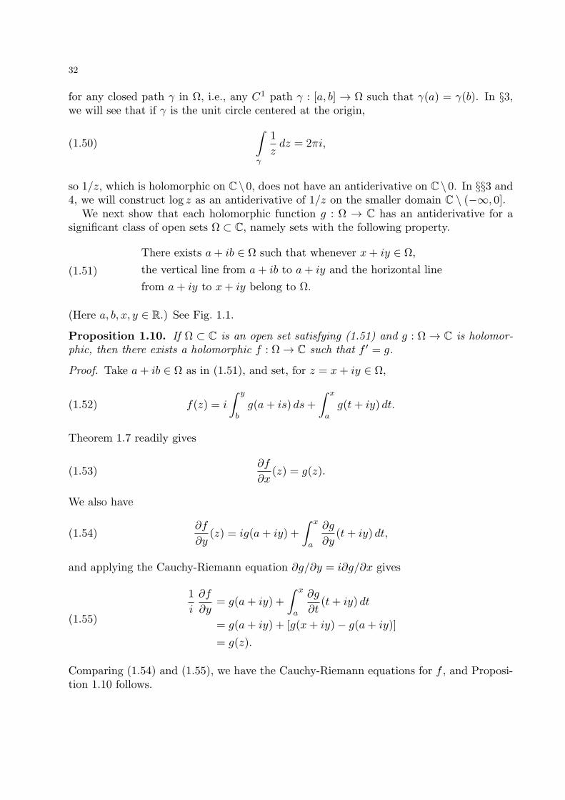
We next show that each holomorphic function g : Ω → C has an antiderivative for asignificant class of open sets Ω ⊂ C, namely sets with the following property.

(1.51)

There exists a+ ib ∈ Ω such that whenever x+ iy ∈ Ω,

the vertical line from a+ ib to a+ iy and the horizontal line

from a+ iy to x+ iy belong to Ω.

(Here a, b, x, y ∈ R.) See Fig. 1.1.

Proposition 1.10. If Ω ⊂ C is an open set satisfying (1.51) and g : Ω → C is holomor-phic, then there exists a holomorphic f : Ω → C such that f ′ = g.

Proof. Take a+ ib ∈ Ω as in (1.51), and set, for z = x+ iy ∈ Ω,

(1.52) f(z) = i

∫ y

b

g(a+ is) ds+

∫ x

a

g(t+ iy) dt.

Theorem 1.7 readily gives

(1.53)∂f

∂x(z) = g(z).

We also have

(1.54)∂f

∂y(z) = ig(a+ iy) +

∫ x

a

∂g

∂y(t+ iy) dt,

and applying the Cauchy-Riemann equation ∂g/∂y = i∂g/∂x gives

(1.55)

1

i

∂f

∂y= g(a+ iy) +

∫ x

a

∂g

∂t(t+ iy) dt

= g(a+ iy) + [g(x+ iy)− g(a+ iy)]

= g(z).

Comparing (1.54) and (1.55), we have the Cauchy-Riemann equations for f , and Proposi-tion 1.10 follows.

33

Examples of open sets satisfying (1.51) include disks and rectangles, while C \ 0 doesnot satisfy (1.51), as one can see by taking a+ ib = −1, x+ iy = 1.

In §7 we extend the conclusion of Proposition 1.10 to a larger class of open sets Ω ⊂ C,called simply connected. See Exercise 8 of §7.

Exercises

1. Let f, g ∈ C1(Ω), not necessarily holomorphic. Show that

(1.56)

∂

∂x(f(z)g(z)) = fx(z)g(z) + f(z)gx(z),

∂

∂y(f(z)g(z)) = fy(z)g(z) + f(z)gy(z),

on Ω, where fx = ∂f/∂x, etc.

2. In the setting of Exercise 1, show that, on z ∈ Ω : g(z) = 0,

(1.57)∂

∂x

1

g(z)= −gx(z)

g(z)2,

∂

∂y

1

g(z)= −gy(z)

g(z)2.

Derive formulas for∂

∂x

f(z)

g(z)and

∂

∂y

f(z)

g(z).

3. In (a)–(d), compute ∂f/∂x and ∂f/∂y. Determine whether f is holomorphic (and onwhat domain). If it is holomorphic, specify f ′(z).

f(z) =z + 1

z2 + 1,(a)

f(z) =z + 1

z2 + 1,(b)

f(z) = e1/z,(c)

f(z) = e−|z|2 .(d)

4. Find the antiderivative of each of the following functions.

f(z) =1

(z + 3)2,(a)

f(z) = zez2

,(b)

f(z) = z2 + ez,(c)

34

5. Let γ : [−1, 1] → C be given by

γ(t) = t+ it2.

Compute∫γf(z) dz in the following cases.

f(z) = z,(a)

f(z) = z,(b)

f(z) =1

(z + 5)2,(c)

f(z) = ez.(d)

6. Do Exercise 5 withγ(t) = t4 + it2.

7. Recall the definition (1.44) for∫γf(z) dz when f ∈ C(Ω) and γ : [a, b] → Ω is a C1

curve. Suppose s : [a, b] → [α, β] is C1, with C1 inverse, such that s(a) = α, s(b) = β. Setσ(s(t)) = γ(t). Show that ∫

γ

f(z) dz =

∫σ

f(ζ) dζ,

so path integrals are invariant under change of parametrization.

In the following exercises, let

∆hf(z) =1

h(f(z + h)− f(z)).

8. Show that ∆hz−1 → −z−2 uniformly on z ∈ C : |z| > ε, for each ε > 0.

Hint. Use (1.10).

9. Let Ω ⊂ C be open and assume K ⊂ Ω is compact. Assume f, g ∈ C(Ω) and

∆hf(z) → f ′(z), ∆hg(z) → g′(z), uniformly on K.

Show that∆h(f(z)g(z)) −→ f ′(z)g(z) + f(z)g′(z), uniformly on K.

Hint. Write∆h(fg)(z) = ∆hf(z) · g(z + h) + f(z)∆hg(z).

35

10. Show that, for each ε > 0, A <∞,

∆hz−n −→ −nz−(n+1)

uniformly on z ∈ C : ε < |z| ≤ A.Hint. Use induction.

11. Let

f(z) =

∞∑k=0

akzk,

and assume this converges for |z| < R, so, by Propositions 0.2–0.3, f is continuous on DR.Show that f is complex-differentiable at 0 and f ′(0) = a1.Hint. Write

f(z) = a0 + a1z + z2∞∑k=0

ak+2zk,

and show that Propositions 0.2–0.3 apply to g(z) =∑∞k=0 ak+2z

k, for |z| < R.

12. Using (1.34)–(1.38), show that if f : Ω → C is a C1 map, each of the following identitiesis equivalent to the condition that f be holomorphic on Ω:

Df =∂u

∂xI +

∂v

∂xJ,

Df =∂v

∂yI − ∂u

∂yJ.

13. For another approach to showing that ez is holomorphic and (d/dz)ez = ez, use (0.60)to write ez = exeiy, with z = x+ iy. Then use (0.51) to show that

∂

∂xex+iy = exeiy, and

∂

∂yex+iy = iexeiy,

so the Cauchy-Riemann equation (1.28) holds, and Proposition 1.5 applies.

14. Let O,Ω be open in C. Assume u : O → Ω is C1 (but not necessarily holomorphic),and f : Ω → C is holomorphic. Show that

∂

∂xf u(z) = f ′(u(z))

∂u

∂x(z),

∂

∂yf u(z) = f ′(u(z))

∂u

∂y(z).

36

2. Holomorphic functions defined by power series

A power series has the form

(2.1) f(z) =

∞∑n=0

an(z − z0)n.

Recall from §0 that to such a series there is associated a radius of convergence R ∈ [0,∞],with the property that the series converges absolutely whenever |z − z0| < R (if R > 0),and diverges whenever |z − z0| > R (if R <∞). We begin this section by identifying R asfollows:

(2.2)1

R= lim sup

n→∞|an|1/n.

This is established in the following result, which reviews and complements Propositions0.2–0.3.

Proposition 2.1. The series (2.1) converges whenever |z−z0| < R and diverges whenever|z − z0| > R, where R is given by (2.2). If R > 0, the series converges uniformly onz : |z − z0| ≤ R′, for each R′ < R. Thus, when R > 0, the series (2.1) defines acontinuous function

(2.3) f : DR(z0) −→ C,

where

(2.4) DR(z0) = z ∈ C : |z − z0| < R.

Proof. If R′ < R, then there exists N ∈ Z+ such that

n ≥ N =⇒ |an|1/n <1

R′ =⇒ |an|(R′)n < 1.

Thus

(2.5) |z − z0| < R′ < R =⇒ |an(z − z0)n| ≤

∣∣∣z − z0R′

∣∣∣n,for n ≥ N , so (2.1) is dominated by a convergent geometrical series in DR′(z0).

For the converse, we argue as follows. Suppose R′′ > R, so infinitely many |an|1/n ≥1/R′′, hence infinitely many |an|(R′′)n ≥ 1. Then

|z − z0| ≥ R′′ > R =⇒ infinitely many |an(z − z0)n| ≥

∣∣∣z − z0R′′

∣∣∣n ≥ 1,

forcing divergence for |z − z0| > R.The assertions about uniform convergence and continuity follow as in Proposition 0.3.

The following result, which extends Proposition 0.4 from the real to the complex domain,is central to the study of holomorphic functions. A converse will be established in §5, as aconsequence of the Cauchy integral formula.

37

Proposition 2.2. If R > 0, the function defined by (2.1) is holomorphic on DR(z0), withderivative given by

(2.6) f ′(z) =∞∑n=1

nan(z − z0)n−1.

Proof. Absolute convergence of (2.6) on DR(z0) follows as in the proof of Proposition 0.4.Alternatively (cf. Exercise 3 below), we have

(2.7) limn→∞

n1/n = 1 =⇒ lim supn→∞

|nan|1/n = lim supn→∞

|an|1/n,

so the power series on the right side of (2.6) converges locally uniformly onDR(z0), defininga continuous function g : DR(z0) → C. It remains to show that f ′(z) = g(z).

To see this, consider

(2.8) fk(z) =k∑

n=0

an(z − z0)n, gk(z) =

k∑n=1

nan(z − z0)n−1.

We have fk → f and gk → g locally uniformly on DR(z0). By (1.12) we have f ′k(z) = gk(z).Hence it follows from Proposition 1.8 that, for z ∈ DR(z0),

(2.9) fk(z) = a0 +

∫σz

gk(ζ) dζ,

for any path σz : [a, b] → DR(z0) such that σz(a) = z0 and σz(b) = z. Making use of thelocally uniform convergence, we can pass to the limit in (2.9), to get

(2.10) f(z) = a0 +

∫σz

g(ζ) dζ.

Taking σz to approach z horizontally, we have (with z = x+ iy, z0 = x0 + iy0)

f(z) = a0 +

∫ y

y0

g(x0 + it) i dt+

∫ x

x0

g(t+ iy) dt,

and hence

(2.11)∂f

∂x(z) = g(z),

while taking σz to approach z vertically yields

f(z) = a0 +

∫ x

x0

g(t+ iy0) dt+

∫ y

y0

g(x+ it) i dt,

38

and hence

(2.12)∂f

∂y(z) = ig(z).

Thus f ∈ C1(DR(z0)) and it satisfies the Cauchy-Riemann equation, so f is holomorphicand f ′(z) = g(z), as asserted.

Remark. A second proof of Proposition 2.2, not involving integral calculus, is given below,following the treatment of Proposition 2.6.

It is useful to note that we can multiply power series with radius of convergence R > 0.In fact, there is the following more general result on products of absolutely convergentseries.

Proposition 2.3. Given absolutely convergent series

(2.13) A =∞∑n=0

αn, B =∞∑n=0

βn,

we have the absolutely convergent series

(2.14) AB =∞∑n=0

γn, γn =n∑j=0

αjβn−j .

Proof. Take Ak =∑kn=0 αn, Bk =

∑kn=0 βn. Then

(2.15) AkBk =k∑

n=0

γn +Rk

with

(2.16) Rk =∑

(m,n)∈σ(k)

αmβn, σ(k) = (m,n) ∈ Z+ × Z+ : m,n ≤ k,m+ n > k.

Hence

(2.17)

|Rk| ≤∑

m≤k/2

∑k/2≤n≤k

|αm| |βn|+∑

k/2≤m≤k

∑n≤k

|αm| |βn|

≤ A∑n≥k/2

|βn|+B∑

m≥k/2

|αm|,

where

(2.18) A =∞∑n=0

|αn| <∞, B =∞∑n=0

|βn| <∞.

It follows that Rk → 0 as k → ∞. Thus the left side of (2.15) converges to AB and theright side to

∑∞n=0 γn. The absolute convergence of (2.14) follows by applying the same

argument with αn replaced by |αn| and βn replaced by |βn|.

39

Corollary 2.4. Suppose the following power series converge for |z| < R:

(2.19) f(z) =∞∑n=0

anzn, g(z) =

∞∑n=0

bnzn.

Then, for |z| < R,

(2.20) f(z)g(z) =∞∑n=0

cnzn, cn =

n∑j=0

ajbn−j .

The following result, which is related to Proposition 2.3, has a similar proof.

Proposition 2.5. If ajk ∈ C and∑j,k |ajk| < ∞, then

∑j ajk is absolutely convergent

for each k,∑k ajk is absolutely convergent for each j, and

(2.21)∑j

(∑k

ajk

)=

∑k

(∑j

ajk

)=

∑j,k

ajk.

Proof. Clearly the hypothesis implies∑j |ajk| <∞ for each k and

∑k |ajk| <∞ for each

j. It also implies that there exists B <∞ such that

SN =N∑j=0

N∑k=0

|ajk| ≤ B, ∀N.

Now SN is bounded and monotone, so there exists a limit, SN A < ∞ as N ∞. Itfollows that, for each ε > 0, there exists N ∈ Z+ such that∑

(j,k)∈C(N)

|ajk| < ε, C(N) = (j, k) ∈ Z+ × Z+ : j > N or k > N.

Now, whenever M,K ≥ N ,∣∣∣ M∑j=0

( K∑k=0

ajk

)−

N∑j=0

N∑k=0

ajk

∣∣∣ ≤ ∑(j,k)∈C(N)

|ajk|,

so ∣∣∣ M∑j=0

( ∞∑k=0

ajk

)−

N∑j=0

N∑k=0

ajk

∣∣∣ ≤ ∑(j,k)∈C(N)

|ajk|,

and hence ∣∣∣ ∞∑j=0

( ∞∑k=0

ajk

)−

N∑j=0

N∑k=0

ajk

∣∣∣ ≤ ∑(j,k)∈C(N)

|ajk|.

We have a similar result with the roles of j and k reversed, and clearly the two finite sumsagree. It follows that ∣∣∣ ∞∑

j=0

( ∞∑k=0

ajk

)−

∞∑k=0

( ∞∑j=0

ajk

)∣∣∣ < 2ε, ∀ ε > 0,

yielding (2.21).

Using Proposition 2.5, we demonstrate the following.

40

Proposition 2.6. If (2.1) has a radius of convergence R > 0, and z1 ∈ DR(z0), then f(z)has a convergent power series about z1:

(2.22) f(z) =∞∑k=0

bk(z − z1)k, for |z − z1| < R− |z1 − z0|.

The proof of Proposition 2.6 will not use Proposition 2.2, and we can use this resultto obtain a second proof of Proposition 2.2. Shrawan Kumar showed the author thisargument.

Proof of Proposition 2.6. There is no loss in generality in taking z0 = 0, which we will dohere, for notational simplicity. Setting fz1(ζ) = f(z1 + ζ), we have from (2.1)

(2.23)

fz1(ζ) =

∞∑n=0

an(ζ + z1)n

=∞∑n=0

n∑k=0

an

(n

k

)ζkzn−k1 ,

the second identity by the binomial formula (cf. (2.34) below). Now,

(2.24)∞∑n=0

n∑k=0

|an|(n

k

)|ζ|k|z1|n−k =

∞∑n=0

|an|(|ζ|+ |z1|)n <∞,

provided |ζ|+ |z1| < R, which is the hypothesis in (2.22) (with z0 = 0). Hence Proposition2.5 gives

(2.25) fz1(ζ) =

∞∑k=0

( ∞∑n=k

an

(n

k

)zn−k1

)ζk.

Hence (2.22) holds, with

(2.26) bk =∞∑n=k

an

(n

k

)zn−k1 .

This proves Proposition 2.6. Note in particular that

(2.27) b1 =∞∑n=1

nanzn−11 .

41

Second proof of Proposition 2.2. The result (2.22) implies f is complex differentiableat each z1 ∈ DR(z0). In fact, the formula (2.22) yields

f(z1 + h) = b0 + b1h+∞∑k=2

bkhk,

and hence

f ′(z1) = limh→0

f(z1 + h)− f(z1)

h= b1,

and the computation (2.27) translates to (2.6), with z = z1.

Remark. Propositions 2.2 and 2.6 are special cases of the following more general results,which will be established in §5.

Proposition 2.7. Let Ω ⊂ C be open, and assume fk : Ω → C are holomorphic. If fk → flocally uniformly on Ω, then f is holomorphic on Ω and

f ′k −→ f ′ locally uniformly on Ω.

Proposition 2.8. If f : Ω → C is holomorphic, z1 ∈ Ω, and DS(z1) ⊂ Ω, then f is givenby a convergent power series of the form (2.22) on DS(z1).

Both of these propositions follow from the Cauchy integral formula. See Proposition 5.10and Theorem 5.5. These results consequently provide alternative proofs of Propositions2.2 and 2.6.

Exercises

1. Determine the radius of convergence R for each of the following series. If 0 < R < ∞,examine when convergence holds at points on |z| = R.

(a) f1(z) =∞∑n=0

zn

(b) f2(z) =

∞∑n=1

zn

n

(c) f3(z) =∞∑n=1

zn

n2

42

(d) f4(z) =∞∑n=0

zn

n!

(e) f5(z) =

∞∑n=0

zn

2n

(f) f6(z) =∞∑n=0

z2n

2n

2. Using Proposition 2.2, find the power series of the derivatives of each of the functionsin Exercise 1. Show that

f ′2(z) =1

1− z,

zf ′3(z) = f2(z),

f ′4(z) = f4(z).

Also, evaluate

g(z) =

∞∑n=1

nzn.

3. Show that if the power series (2.1) has radius of convergence R > 0, then f ′′, f ′′′, . . .are holomorphic on DR(z0) and

(2.28) f (n)(z0) = n! an.

Here we set f (n)(z) = f ′(z) for n = 1, and inductively f (n+1)(z) = (d/dz)f (n)(z).

4. Given a > 0, show that for n ≥ 1

(2.29) (1 + a)n ≥ 1 + na.

(Cf. Exercise 2 of §0.) Use (2.29) to show that

(2.30) lim supn→∞

n1/n ≤ 1,

and hence

(2.31) limn→∞

n1/n = 1,

a result used in (2.7).Hint. To get (2.30), deduce from (2.29) that n1/n ≤ (1 + a)/a1/n. Then show that, foreach a > 0,

(2.32) limn→∞

a1/n = 1.

43

For another proof of (2.31), see Exercise 4 of §4.

5. The following is a version of the binomial formula. If a ∈ C, n ∈ N,

(2.33) (1 + a)n =n∑k=0

(n

k

)ak,

(n

k

)=

n!

k!(n− k)!.

Another version is

(2.34) (z + w)n =

n∑k=0

(n

k

)zkwn−k.

Verify this identity and show that (2.33) implies (2.29) when a > 0.Hint. To verify (2.34), expand

(2.35) (z + w)n = (z + w) · · · (z + w)

as a sum of monomials and count the number of terms equal to zkwn−k. Use the fact that

(2.36)

(n

k

)= number of combinations of n objects, taken k at a time.

6. As a special case of Exercise 3, note that, given a polynomial

(2.37) p(z) = anzn + · · ·+ a1z + a0,

we have

(2.38) p(k)(0) = k! ak, 0 ≤ k ≤ n.

Apply this to

(2.39) pn(z) = (1 + z)n.

Compute p(k)n (z), using (1.5), then compute p(k)(0), and use this to give another proof of

(2.33), i.e.,

(2.40) pn(z) =

n∑k=0

(n

k

)zk,

(n

k

)=

n!

k!(n− k)!.

44

3. Exponential and trigonometric functions: Euler’s formula

Recall from §§0 and 1 that we define the exponential function by its power series:

(3.1) ez = 1 + z +z2

2!+ · · ·+ zj

j!+ · · · =

∞∑j=0

zj

j!.

By the ratio test this converges for all z, to a continuous function on C. Furthermore, theexponential function is holomorphic on C. This function satisfies

(3.2)d

dzez = ez, e0 = 1.

One derivation of this was given in §1. Alternatively, (3.2) can be established by differen-tiating term by term the series (3.1) to get (by Proposition 2.2)

(3.3)

d

dzez =

∞∑j=1

1

(j − 1)!zj−1 =

∞∑k=0

1

k!zk

=

∞∑k=0

1

k!zk = ez.

The property (3.2) uniquely characterizes ez. It implies

(3.4)dj

dzjez = ez, j = 1, 2, 3, . . . .

By (2.21), any function f(z) that is the sum of a convergent power series about z = 0 hasthe form

(3.5) f(z) =∞∑j=0

f (j)(0)

j!zj ,

which for a function satisfying (3.2) and (3.4) leads to (3.1). A simple extension of (3.2) is

(3.6)d

dzeaz = a eaz.

Note how this also extends (0.51).As shown in (0.60), the exponential function satisfies the fundamental identity

(3.7) ezew = ez+w, ∀ z, w ∈ C.

45

For an alternative proof, we can expand the left side of (3.7) into a double series:

(3.8) ezew =

∞∑j=0

zj

j!

∞∑k=0

wk

k!=

∞∑j,k=0

zjwk

j!k!.

We compare this with

(3.9) ez+w =

∞∑n=0

(z + w)n

n!,

using the binomial formula (cf. (2.34))

(3.10) (z + w)n =n∑j=0

(n

j

)zjwn−j ,

(n

j

)=

n!

j!(n− j)!.

Setting k = n− j, we have

(3.11) ez+w =∞∑n=0

∑j+k=n;j,k≥0

1

n!

n!

j!k!zjwk =

∞∑j,k=0

zjwk

j!k!.

See (2.14) for the last identity. Comparing (3.8) and (3.11) again gives the identity (3.7).We next record some properties of exp(t) = et for real t. The power series (3.1) clearly

gives et > 0 for t ≥ 0. Since e−t = 1/et, we see that et > 0 for all t ∈ R. Sincedet/dt = et > 0, the function is monotone increasing in t, and since d2et/dt2 = et > 0,this function is convex. Note that

(3.12) et > 1 + t, for t > 0.

Hence

(3.13) limt→+∞

et = +∞.

Since e−t = 1/et,

(3.14) limt→−∞

et = 0.

As a consequence,

(3.15) exp : R −→ (0,∞)

is smooth and one-to-one and onto, with positive derivative, so the inverse function theoremof one-variable calculus applies. There is a smooth inverse

(3.16) L : (0,∞) −→ R.

46

We call this inverse the natural logarithm:

(3.17) log x = L(x).

See Figures 3.1 and 3.2 for graphs of x = et and t = log x.Applying d/dt to

(3.18) L(et) = t

gives

(3.19) L′(et)et = 1, hence L′(et) =1

et,

i.e.,

(3.20)d

dxlog x =

1

x.

Since log 1 = 0, we get

(3.21) log x =

∫ x

1

dy

y.

An immediate consequence of (3.7) (for z, w ∈ R) is the identity

(3.22) log xy = log x+ log y, x, y ∈ (0,∞),

which can also be deduced from (3.21).We next show how to extend the logarithm into the complex domain, defining log z for

z ∈ C \ R−, where R− = (−∞, 0], using Proposition 1.10. In fact, the hypothesis (1.51)holds for Ω = C \ R−, with a + ib = 1, so each holomorphic function g on C \ R− has aholomorphic anti-derivative. In particular, 1/z has an anti-derivative, and this yields

(3.22A) log : C \ R− → C,d

dzlog z =

1

z, log 1 = 0.

By Proposition 1.8, we have

(3.22B) log z =

∫ z

1

dζ

ζ,

the integral taken along any path in C\R− from 1 to z. Comparison with (3.21) shows thatthis function restricted to (0,∞) coincides with log as defined in (3.17). In §4 we displaylog in (3.22A) as the inverse of the exponential function exp(z) = ez on the domainΣ = x + iy : x ∈ R, y ∈ (−π, π), making use of some results that will be derived next.(See also Exercises 13–15 at the end of this section.)

47

We move next to a study of ez for purely imaginary z, i.e., of

(3.23) γ(t) = eit, t ∈ R.

This traces out a curve in the complex plane, and we want to understand which curve itis. Let us set

(3.24) eit = c(t) + is(t),

with c(t) and s(t) real valued. First we calculate |eit|2 = c(t)2 + s(t)2. For x, y ∈ R,

(3.25) z = x+ iy =⇒ z = x− iy =⇒ zz = x2 + y2 = |z|2.

It is elementary that

(3.26)z, w ∈ C =⇒ zw = z w =⇒ zn = zn,

and z + w = z + w.

Hence

(3.27) ez =∞∑k=0

zk

k!= ez.

In particular,

(3.28) t ∈ R =⇒ |eit|2 = eite−it = 1.

Hence t 7→ γ(t) = eit has image in the unit circle centered at the origin in C. Also

(3.29) γ′(t) = ieit =⇒ |γ′(t)| ≡ 1,

so γ(t) moves at unit speed on the unit circle. We have

(3.30) γ(0) = 1, γ′(0) = i.

Thus, for t between 0 and the circumference of the unit circle, the arc from γ(0) to γ(t) isan arc on the unit circle, pictured in Figure 3.3, of length

(3.31) ℓ(t) =

∫ t

0

|γ′(s)| ds = t.

Standard definitions from trigonometry say that the line segments from 0 to 1 and from0 to γ(t) meet at angle whose measurement in radians is equal to the length of the arc ofthe unit circle from 1 to γ(t), i.e., to ℓ(t). The cosine of this angle is defined to be the

48

x-coordinate of γ(t) and the sine of the angle is defined to be the y-coordinate of γ(t).Hence the computation (3.31) gives

(3.32) c(t) = cos t, s(t) = sin t.

Thus (3.24) becomes

(3.33) eit = cos t+ i sin t,

an identity known as Euler’s formula. The identity

(3.34)d

dteit = ieit,

applied to (3.33), yields

(3.35)d

dtcos t = − sin t,

d

dtsin t = cos t.

We can use (3.7) to derive formulas for sin and cos of the sum of two angles. Indeed,comparing

(3.36) ei(s+t) = cos(s+ t) + i sin(s+ t)

with

(3.37) eiseit = (cos s+ i sin s)(cos t+ i sin t)

gives

(3.38)cos(s+ t) = (cos s)(cos t)− (sin s)(sin t),

sin(s+ t) = (sin s)(cos t) + (cos s)(sin t).

Derivations of the formulas (3.35) for the derivative of cos t and sin t given in firstsemester calculus courses typically make use of (3.38) and further limiting arguments,which we do not need with the approach used here.

A standard definition of the number π is half the length of the unit circle. Hence π isthe smallest positive number such that γ(2π) = 1. We also have

(3.39) γ(π) = −1, γ(π2

)= i.

Furthermore, consideration of Fig. 3.4 shows that

(3.40) γ(π3

)=

1

2+

√3

2i, γ

(π6

)=

√3

2+

1

2i.

49

We now show how to compute an accurate approximation to π.This formula will arise by comparing two ways to compute the length of an arc of a

circle. So consider the length of γ(t) over 0 ≤ t ≤ φ. By (3.29) we know it is equal to φ.Suppose 0 < φ < π/2 and parametrize this segment of the circle by

(3.41) σ(s) = (√

1− s2, s), 0 ≤ s ≤ τ = sin φ.

Then we know the length is also given by

(3.42) ℓ =

∫ τ

0

|σ′(s)| ds =∫ τ

0

ds√1− s2

.

Comparing these two length calculations, we have

(3.43)

∫ τ

0

ds√1− s2

= φ, sin φ = τ,

when 0 < φ < π/2. As another way to see this, note that the substitution s = sin θ gives,

by (3.35), ds = cos θ dθ, while√1− s2 = cos θ by (3.28), which implies

(3.44) cos2 t+ sin2 t = 1.

Thus

(3.45)

∫ τ

0

ds√1− s2

=

∫ φ

0

dθ = φ,

again verifying (3.43).In particular, using sin(π/6) = 1/2, from (3.40), we deduce that

(3.46)π

6=

∫ 1/2

0

dx√1− x2

.

One can produce a power series for (1 − y)−1/2 and substitute y = x2. (For more onthis, see the exercises at the end of §5.) Integrating the resulting series term by term, oneobtains

(3.47)π

6=

∞∑n=0

an2n+ 1

(12

)2n+1

,

where the numbers an are defined inductively by

(3.48) a0 = 1, an+1 =2n+ 1

2n+ 2an.

50

Using a calculator, one can sum this series over 0 ≤ n ≤ 20 and show that

(3.49) π = 3.141592653589 · · · .

We leave the verification of (3.47)–(3.49) as an exercise, once one gets to Exercises 1–2 of§5.

Exercises

Here’s another way to demonstrate the formula (3.35) for the derivatives of sin t and cos t.

1. Suppose you define cos t and sin t so that γ(t) = (cos t, sin t) is a unit-speed parametriza-tion of the unit circle centered at the origin, satisfying γ(0) = (1, 0), γ′(0) = (0, 1), (as wedid in (3.32)). Show directly (without using (3.35)) that

γ′(t) = (− sin t, cos t),

and hence deduce (3.35). (Hint. Differentiate γ(t) · γ(t) = 1 to deduce that, for eacht, γ′(t) ⊥ γ(t). Meanwhile, |γ(t)| = |γ′(t)| = 1.)

2. It follows from (3.33) and its companion e−it = cos t− i sin t that

(3.50) cos z =eiz + e−iz

2, sin z =

eiz − e−iz

2i

for z = t ∈ R. We define cos z and sin z as holomorphic functions on C by these identities.Show that they yield the series expansions

(3.51) cos z =∞∑k=0

(−1)k

(2k)!z2k, sin z =

∞∑k=0

(−1)k

(2k + 1)!z2k+1.

3. Extend the identities (3.35) and (3.38) to complex arguments. In particular, for z ∈ C,we have

(3.52)cos(z + π

2 ) = − sin z, cos(z + π) = − cos z, cos(z + 2π) = cos z,

sin(z + π2 ) = cos z, sin(z + π) = − sin z, sin(z + 2π) = sin z.

4. We define

(3.53) cosh y =ey + e−y

2, sinh y =

ey − e−y

2.

Show that cos iy = cosh y, sin iy = i sinh y, and hence

(3.54)cos(x+ iy) = cosx cosh y − i sinx sinh y,

sin(x+ iy) = sinx cosh y + i cosx sinh y.

51

5. Define tan z for z = (k + 1/2)π and cot z for z = kπ, k ∈ Z, by

(3.55) tan z =sin z

cos z, cot z =

cos z

sin z.

Show that

(3.56) tan(z + π2 ) = − cot z, tan(z + π) = tan z,

and

(3.57)d

dztan z =

1

cos2 z= 1 + tan2 z.

6. For each of the following functions g(z), find a holomorphic function f(z) such thatf ′(z) = g(z).

a) g(z) = zkez, k ∈ Z+.b) g(z) = eaz cos bz.

7. Concerning the identities in (3.40), verify algebraically that

(12+

√3

2i)3

= −1.

Then use eπi/6 = eπi/2e−πi/3 to deduce the stated identity for γ(π/6) = eπi/6.

8. Let γ be the unit circle centered at the origin in C, going counterclockwise. Show that∫γ

1

zdz =

∫ 2π

0

ieit

eitdt = 2πi,

as stated in (1.50).

9. One sets

sec z =1

cos z,

so (3.57) yields (d/dz) tan z = sec2 z. Where is sec z holomorphic? Show that

d

dzsec z = sec z tan z.

10. Show that1 + tan2 z = sec2 z.

52

11. Show thatd

dz(sec z + tan z) = sec z (sec z + tan z),

andd

dz(sec z tan z) = sec z tan2 z + sec3 z

= 2 sec3 z − sec z.

(Hint. Use Exercise 10 for the last identity.)

12. The identities (3.53) serve to define cosh y and sinh y for y ∈ C, not merely for y ∈ R.Show that

d

dzcosh z = sinh z,

d

dzsinh z = cosh z,

andcosh2 z − sinh2 z = 1.

The next exercises present log, defined on C \R− as in (3.22A), as the inverse function tothe exponential function exp(z) = ez, by a string of reasoning different from what we willuse in §4. In particular, here we avoid having to appeal to the inverse function theorem,Theorem 4.2. Set

(3.58) Σ = x+ iy : x ∈ R, y ∈ (−π, π).

13. Using ex+iy = exeiy and the properties of exp : R → (0,∞) and of γ(y) = eiy

established in (3.15) and (3.33), show that

(3.59) exp : Σ −→ C \ R− is one-to-one and onto.

14. Show that

(3.60) log(ez) = z ∀ z ∈ Σ.

Hint. Apply the chain rule to compute g′(z) for g(z) = log(ez). Note that g(0) = 0.

15. Deduce from Exercises 13 and 14 that

log : C \ R− −→ Σ

is one-to-one and onto, and is the inverse to exp in (3.59).

53

4. Square roots, logs, and other inverse functions

We recall the Inverse Function Theorem for functions of real variables.

Theorem 4.1. Let Ω ⊂ Rn be open and let f : Ω → Rn be a C1 map. Take p ∈ Ωand assume Df(p) is an invertible linear transformation on Rn. Then there exists aneighborhood O of p and a neighborhood U of q = f(p) such that f : O → U is one-to-oneand onto, the inverse g = f−1 : U → O is C1, and, for x ∈ O, y = f(x),

(4.1) Dg(y) = Df(x)−1.

A proof of this is given in Appendix B. This result has the following consequence, whichis the Inverse Function Theorem for holomorphic functions.

Theorem 4.2. Let Ω ⊂ C be open and let f : Ω → C be holomorphic. Take p ∈ Ωand assume f ′(p) = 0. Then there exists a neighborhood O of p and a neighborhood U ofq = f(p) such that f : O → U is one-to-one and onto, the inverse g = f−1 : U → O isholomorphic, and, for z ∈ O, w = f(z),

(4.2) g′(w) =1

f ′(z).

Proof. If we check that g is holomorphic, then (4.2) follows from the chain rule, Proposition1.2, applied to

g(f(z)) = z.

We know g is C1. By Proposition 1.6, g is holomorphic on U if and only if, for each w ∈ U ,Dg(w) commutes with J , given by (1.39). Also Proposition 1.6 implies Df(z) commuteswith J . To finish, we need merely remark that if A is an invertible 2× 2 matrix,

(4.3) AJ = JA⇐⇒ A−1J = JA−1.

As a first example, consider the function Sq(z) = z2. Note that we can use polarcoordinates, (x, y) = (r cos θ, r sin θ), or equivalently z = reiθ, obtaining z2 = r2e2iθ. Thisshows that Sq maps the right half-plane

(4.4) H = z ∈ C : Re z > 0

bijectively onto C \ R− (where R− = (−∞, 0]). Since Sq′(z) = 2z vanishes only at z = 0,we see that we have a holomorphic inverse

(4.5) Sqrt : C \ R− −→ H,

54

given by

(4.6) Sqrt(reiθ) = r1/2eiθ/2, r > 0, −π < θ < π.

We also write

(4.7)√z = z1/2 = Sqrt(z).

We will occasionally find it useful to extend Sqrt to

Sqrt : C −→ C,

defining Sqrt on (−∞, 0] by Sqrt(−x) = i√x, for x ∈ [0,∞). This extended map is

discontinuous on (−∞, 0).We can define other non-integral powers of z on C\R−. Before doing so, we take a look

at log, the inverse function to the exponential function, exp(z) = ez. Consider the strip

(4.8) Σ = x+ iy : x ∈ R, −π < y < π.

Since ex+iy = exeiy, we see that we have a bijective map

(4.9) exp : Σ −→ C \ R−.

Note that dez/dz = ez is nowhere vanishing, so (4.9) has a holomorphic inverse we denotelog:

(4.10) log : C \ R− −→ Σ.

Note that

(4.11) log 1 = 0.

Applying (4.2) we have

(4.12)d

dzez = ez =⇒ d

dzlog z =

1

z.

Thus, applying Proposition 1.8, we have

(4.13) log z =

∫ z

1

1

ζdζ,

where the integral is taken along any path from 1 to z in C\R−. Comparison with (3.22B)shows that the function log produced here coincides with the function arising in (3.22A).(This result also follows from Exercises 13–15 of §3.)

55

Now, given any a ∈ C, we can define

(4.14) za = Powa(z), Powa : C \ R− → C

by

(4.15) za = ea log z.

The identity eu+v = euev then gives

(4.16) za+b = zazb, a, b ∈ C, z ∈ C \ R−.

In particular, for n ∈ Z, n = 0,

(4.17) (z1/n)n = z.

Making use of (4.12) and the chain rule (1.20), we see that

(4.18)d

dzza = a za−1.

While Theorem 4.1 and Corollary 4.2 are local in nature, the following result can provideglobal inverses, in some important cases.

Proposition 4.3. Suppose Ω ⊂ C is convex. Assume f is holomorphic in Ω and thereexists a ∈ C such that

Re af ′ > 0 on Ω.

Then f maps Ω one-to-one onto its image f(Ω).

Proof. Consider distinct points z0, z1 ∈ Ω. The convexity implies the line σ(t) = (1 −t)z0 + tz1 is contained in Ω, for 0 ≤ t ≤ 1. By Proposition 1.8, we have

(4.19) af(z1)− f(z0)

z1 − z0=

∫ 1

0

af ′((1− t)z0 + tz1

)dt,

which has positive real part and hence is not zero.

As an example, consider the strip

(4.20) Σ =x+ iy : −π

2< x <

π

2, y ∈ R

.

Take f(z) = sin z, so f ′(z) = cos z. It follows from (3.54) that

(4.21) Re cos z = cosx cosh y > 0, for z ∈ Σ,

56

so f maps Σ one-to-one onto its image. Note that

(4.22) sin z = g(eiz), where g(ζ) =1

2i

(ζ − 1

ζ

),

and the image of Σ under z 7→ eiz is the right half plane H, given by (4.4). Below we willshow that the image of H under g is

(4.23) C \ (−∞,−1] ∪ [1,∞).

It then follows that sin maps Σ one-to-one onto the set (4.23). The inverse function isdenoted sin−1:

(4.24) sin−1 : C \ (−∞,−1] ∪ [1,∞) −→ Σ.

We have sin2 z ∈ C \ [1,∞) for z ∈ Σ, and it follows that

(4.25) cos z = (1− sin2 z)1/2, z ∈ Σ.

Hence, by (4.2), g(z) = sin−1 z satisfies

(4.26) g′(z) = (1− z2)−1/2, z ∈ C \ (−∞,−1] ∪ [1,∞),

and hence, by Proposition 1.8,

(4.27) sin−1 z =

∫ z

0

(1− ζ2)−1/2 dζ,

where the integral is taken along any path from 0 to z in C\(−∞,−1]∪ [1,∞). Comparethis identity with (3.43), which treats the special case of real z ∈ (−1, 1).

It remains to prove the asserted mapping property of g, given in (4.22). We rephrasethe result for

(4.28) h(ζ) = g(iζ) =1

2

(ζ +

1

ζ

).

Proposition 4.4. The function h given by (4.28) maps both the upper half plane U =ζ : Im ζ > 0 and the lower half plane U∗ = ζ : Im ζ < 0, one-to-one onto

C \ (−∞,−1] ∪ [1,∞).

Proof. Note that h : C \ 0 → C, and

(4.29) h(1ζ

)= h(ζ).

57

Taking w ∈ C, we want to solve h(ζ) = w for ζ. This is equivalent to

(4.30) ζ2 − 2wζ + 1 = 0,

with solutions

(4.31) ζ = w ±√w2 − 1.

Thus, for each w ∈ C, there are two solutions, except for w = ±1, with single solutionsh(−1) = −1, h(1) = 1. If we examine h(x) for x ∈ R \ 0 (see Fig. 4.1), we see that h mapsR \ 0 onto (−∞,−1] ∪ [1,∞), 2-to-1 except at x = ±1. It follows that, given ζ ∈ C \ 0,h(ζ) = w belongs to (−∞,−1]∪ [1,∞) if and only if ζ ∈ R. If w belongs to the set (4.23),i.e., if w ∈ C \ (−∞,−1] ∪ [1,∞), then h(ζ) = w has two solutions, both in C \ R, andby (4.29) they are reciprocals of each other. Now

(4.32)1

ζ=

ζ

|ζ|2,

so, given ζ ∈ C \ R, we have ζ ∈ U ⇔ 1/ζ ∈ U∗. This proves Proposition 4.4.

Exercises

1. Show that, for |z| < 1,

(4.33) log(1 + z) =∞∑n=1

(−1)n−1 zn

n.

Hint. Use (4.13) to write

log(1 + z) =

∫ z

0

1

1 + ζdζ,

and plug in the power series for 1/(1 + ζ).

2. Using Exercise 1 (plus further arguments), show that

(4.34)

∞∑n=1

(−1)n−1

n= log 2.

Hint. Using properties of alternating series, show that, for r ∈ (0, 1),

(4.34A)N∑n=1

(−1)n−1

nrn = log(1 + r) + εN (r), |εN (r)| ≤ rN+1

N + 1.

58

Then let r → 1 in (4.34A).

3. Take x ∈ (0,∞). Show that

limx→∞

log x

x= 0.

Hint. If x = ey, (log x)/x = ye−y.

4. Using Exercise 3, show thatlim

x→+∞x1/x = 1.

Note that this contains the result (2.31).Hint. x1/x = e(log x)/x.

5. Write the Euler identity as

eiw =√

1− z2 + iz, z = sinw,

for w near 0. Deduce that

(4.35) sin−1 z =1

ilog

(√1− z2 + iz

), |z| < 1.

Does this extend to C \ (−∞,−1] ∪ [1,∞)?

6. Compute the following quantities:

a) i1/2,b) i1/3,c) ii.

7. Show that tan z maps the strip Σ given by (4.20) diffeomorphically onto

(4.36) C \ (−∞,−1]i ∪ [1,∞)i.

Hint. Consult Fig. 4.2. To get the last step, it helps to show that

R(z) =1− z

1 + z

has the following properties:(a) R : C \ −1 → C \ −1, and R(z) = w ⇔ z = R(w),(b) R : R \ −1 → R \ −1,(c) R : (0,∞) → (−1, 1),and in each case the map is one-to-one and onto.

59

8. Making use of (3.57), show that on the region (4.36) we have

(4.37) tan−1 z =

∫ z

0

dζ

1 + ζ2,

where tan−1 is the inverse of tan in Exercise 7, and the integral is over any path from 0 toz within the region (4.36). Writing (1 + ζ2)−1 as a geometric series and integrating termby term, show that

(4.37A) tan−1 z =

∞∑k=0

(−1)kz2k+1

2k + 1. for |z| < 1.

Use the fact that

(4.37B) tanπ

6=

√3

4

to obtain

(4.37C)π

6=

√3

4

∞∑k=0

(−1)k

2k + 1

( 3

16

)k.

Compare the series (3.47). See Exercise 29 below for an approach to evaluating√3. How

many terms in (4.37C) do you need to obtain 16 digits of accuracy?

9. Show thatd

dzlog sec z = tan z.

On what domain in C does this hold?

10. Using Exercise 11 of §3, compute

d

dzlog(sec z + tan z),

and find the antiderivatives ofsec z and sec3 z.

On what domains do the resulting formulas work?

11. Consider the integral

(4.38) I(u) =

∫ u

0

dt√1 + t2

,

60

with u ∈ R.

(a) Use the change of variable t = sinh v to show that

I(sinh v) = v.

(b) Use the change of variable t = tanx to show that

I(tanx) =

∫ x

0

sec s ds, −π2< x <

π

2.

(c) Deduce from (a) and (b) that∫ x

0

sec s ds = sinh−1(tanx), −π2< x <

π

2.

(d) Use the last identity to show that

cosh(∫ x

0

sec s ds)= secx.

Compare the last results with conclusions of Exercise 10.

12. As a variant of (4.20)–(4.23), show that z 7→ sin z mapsx+ iy : −π

2< x <

π

2, y > 0

one-to-one and onto the upper half plane z : Im z > 0.

The next exercises construct the holomorphic inverse to sin on the set

(4.39) Ω = C \ (−∞,−1] ∪ [1,∞),

satisfying (4.27), in a manner that avoids appeal to Theorem 4.2. (Compare the con-struction of log as an inverse to exp in Exercises 13–15 of §3.) We will use the resultthat

(4.40) sin : Σ −→ Ω is one-to-one and onto,

with Σ as in (4.20), established above via Proposition 4.4.

13. Show that, for Ω as in (4.39),

z ∈ Ω ⇒ z2 ∈ C \ [1,∞) ⇒ 1− z2 ∈ C \ (−∞, 0],

61

and deduce that the function f(z) = (1− z2)−1/2 is holomorphic on Ω.

14. Show that the set Ω in (4.39) satisfies the hypotheses of Proposition 1.10, with a+ ib =0. Deduce that the function f(z) = (1 − z2)−1/2 has a holomorphic anti-derivative G onΩ:

(4.41) G : Ω → C, G′(z) = (1− z2)−1/2, G(0) = 0.

Deduce from Proposition 1.8 that

(4.42) G(z) =

∫ z

0

(1− ζ2)−1/2 dζ, z ∈ Ω,

the integral taken along any path in Ω from 0 to z.

15. Show that

(4.43) G(sin z) = z, ∀ z ∈ Σ.

Hint. Apply the chain rule to f(z) = G(sin z), making use of (4.25), to show that f ′(z) = 1

for all z ∈ Σ.

16. Use (4.40) and Exercise 15 to show that

(4.44) G : Ω −→ Σ is one-to-one and onto,

and is the holomorphic inverse to sin in (4.40).

17. Expanding on Proposition 4.4, show that the function h, given by (4.28), has thefollowing properties:(a) h : C \ 0 → C is onto,(b) h : C \ 0, 1,−1 → C \ 1,−1 is two-to-one and onto,(c) h : R \ 0 → R \ (−1, 1) is onto, and is two-to-one, except at x = ±1.

18. Given a ∈ C \ R−, set

Ea(z) = az = ez log a, z ∈ C.

Show that Ea is holomorphic in z and compute E′a(z).

19. Deduce from Exercise 1 that

∞∑n=1

zn−1

n= λ(z), for |z| < 1,

62

where

λ(z) = − log(1− z)

z, for 0 < |z| < 1,

1 for z = 0.

Use this to show that∞∑n=1

zn

n2=

∫ z

0

1

ζlog

1

1− ζdζ,

for |z| < 1, where the integral is taken along any path from 0 to z in the unit disk D1(0).

20. Show that

limk→∞

k∑ℓ=−k

1

k + iℓ=

∫ 1

−1

dz

1 + iz=π

2.

21. Show that, for x > 0,

logx+ i

x− i= 2i tan−1 1

x

22. Show that, for x > 0, ∫ x

0

log t dt = x log x− x.

23. Show that, for x > 0, a ∈ C \ (−∞, 0],∫ x

0

log(t+ a) dt = (x+ a) log(x+ a)− x− a log a.

Show that ∫ x

0

log(t2 + 1) dt = x log(x2 + 1) + i logx+ i

x− i− 2x+ π.

Compute ∫ x

0

log(1 +

1

t2

)dt,

and show that ∫ ∞

0

log(1 +

1

t2

)dt = π.

24. Take the following path to explicitly finding the real and imaginary parts of a solutionto

z2 = a+ ib,

given a+ ib /∈ R−. Namely, with x = Re z, y = Im z, we have

x2 − y2 = a, 2xy = b,

63

and also

x2 + y2 = ρ =√a2 + b2,

hence

x =

√ρ+ a

2, y =

b

2x.

Exercises 25–27 deal with a method of solving

(4.45) z3 = α = 1 + β,

given a restriction on the size of β ∈ C.

25. As a first approximation to a solution to (4.45), take ζ0 = 1 + β/3, so

ζ30 = 1 + β +β2

3+β3

27

= α+β2

3

(1 +

β

9

).

Now set

z =(1 +

β

3

)z−11 ,

and show that solving (4.45) is equivalent to solving

(4.46)

z31 = 1 +1

α

(β2

3+β3

27

)= 1 + β1

= α1,

where the last 2 identities define β1 and α1.

26. Apply the procedure of Exercise 25 to the task of solving z31 = α1 = 1 + β1. Set

z1 =(1 +

β13

)z−12 ,

so solving (4.46) is equivalent to solving

z32 = 1 +1

α1

(β21

3+β31

27

)= 1 + β2

= α2.

64

Continue this process, obtaining that (4.45) is equivalent to

(4.47) z =(1 +

β

3

)(1 +

β13

)−1

· · ·(1 +

βk3

)σ(k)z−1k+1,

with β(k) = (−1)k and zk+1 solving

z3k+1 = 1 +1

αk

β2k

3

(1 +

βk9

)= 1 + βk+1

= αk+1.

27. With βk as in (4.48), show that

|βk| ≤1

2⇒ |αk| ≥

1

2

⇒ |βk+1 ≤ 19

27|βk|2,

and

|βk| ≤1

4⇒ |αk| ≥

3

4

⇒ |βk+1| ≤1

2|βk|2.

Use this to establish the following.

Assertion. Assume

|β| ≤ 1

2, α = 1 + β,

and form the sequence β1, . . . , βk, . . . , as in Exercises 25–26, i.e.,

β1 =1

α

β2

3

(1 +

β

9

), α1 = 1 + β1,

βk+1 =1

αk

β2k

3

(1 +

βk9

), αk+1 = 1 + βk+1.

Then the sequence

ζk =(1 +

β

3

)(1 +

β13

)−1

· · ·(1 +

βk3

)σ(k)converges as k → ∞ to α1/3.

Note that an equivalent description of ζk is

ζ0 = 1 +β

3,

ζk = ζk−1

(1 +

βk3

)σ(k).

65

28. Take k ∈ N, k ≥ 2. Extend the method of Exercises 25–27 to approximate a solutionto

zk = α = 1 + β,

given a restriction on the size of β.

Exercises 29–33 are recommended for the reader able to use a computer or calculator fornumerical work.

29. Here is an alternative method of approximating√α, given α ∈ C \ (−∞, 0]. Suppose

you have an approximation ζk,ζk −

√α = δk.

Square this to obtain ζ2k + α− 2ζk√α = δ2k, hence

√α =

α+ ζ2k2ζk

− δ2k2ζk

.

Hence

ζk+1 =α+ ζ2k2ζk

is an improved approximation, as long as |δk| < 2|ζk|. One can iterate this. Try it on

√2 ≈ 7

5,

√3 ≈ 7

4,

√5 ≈ 9

4.

How many iterations does it take to approximate these quantities to 16 digits of accuracy?

30. Given that

eπi/6 =

√3

2+i

2,

eπi/4 =1 + i√

2, and

eπi/12 = eπi/4e−πi/6,

use the method of Exercise 27 to obtain an accurate numerical evaluation of

eπi/36 = cosπ

36+ i sin

π

36.

How many iterations does it take to approximate this quantity to 16 digits of accuracy?

31. Peek at (Q.32) to see that

cos2π

5=

√5− 1

4.

66

Use this to obtain an accurate numerical evaluation of

e2πi/5 = cos2π

5+ i sin

2π

5,

and from this ofeπi/5 = −e−4πi/5, and

eπi/30 = eπi/5e−πi/6.

Then use the method of Exercise 27 to obtain an accurate numerical evaluation of

eπi/90 = cosπ

90+ i sin

π

90.

32. Apply Exercise 28 or 29 to α = eπi/90, to give an accurate numerical evaluation of

eπi/180 = cosπ

180+ i sin

π

180= cos 1 + i sin 1.

If you use Exercise 29, take ζ1 = (1 + α)/2. Alternatively, apply Exercise 28, with k = 6,to α = eπi/30.Using these calculations, evaluate

(4.49) tanπ

180= δ.

33. Substitute δ in (4.49) into

(4.50) tan−1 x =∞∑k=0

(−1)kx2k+1

2k + 1, |x| < 1,

from (4.37A), to obtain

(4.51)

π

180=

∞∑k=0

(−1)kδ2k+1

2k + 1

= δ − δ3

3+δ5

5− · · · .

Show that

δ − δ3

3<

π

180< δ.

How many terms in the series (4.51) are needed to obtain π to 16 digits of accuracy,assuming the evaluation of δ is sufficiently accurate?

Similarly, apply (4.50) to the following quantities, whose evaluations are available fromthe results of Exercises 30–31.

tanπ

12= δ1 = 2−

√3,

tanπ

30= δ2,

tanπ

36= δ3.

Compare the approach to evaluating π described in Exercise 8.

67

I. π2 is Irrational

The following proof that π2 is irrational follows a classic argument of I. Niven, [Niv].The idea is to consider

(I.1) In =

∫ π

0

φn(x) sinx dx, φn(x) =1

n!xn(π − x)n.

Clearly In > 0 for each n ∈ N, and In → 0 very fast, faster than geometrically. The nextkey fact is that In is a polynomial of degree n in π2 with integer coefficients:

(I.2) In =n∑k=0

cnkπ2k, cnk ∈ Z.

Given this it follows readily that π2 is irrational. In fact, if π2 = a/b, a, b ∈ N, then

(I.3)

n∑k=0

cnka2kb2n−2k = b2nIn.

But the left side of (I.3) is an integer for each n, while by the estimate on (I.1) mentionedabove the right side belongs to the interval (0, 1) for large n, yielding a contradiction. Itremains to establish (I.2).

A method of computing the integral in (I.1), which works for any polynomial φn(x)) isthe following. One looks for an antiderivative of the form

(I.4) Gn(x) sinx− Fn(x) cosx,

where Fn and Gn are polynomials. One needs

(I.5) Gn(x) = F ′n(x), G′

n(x) + Fn(x) = φn(x),

hence

(I.6) F ′′n (x) + Fn(x) = φn(x).

One can exploit the nilpotence of ∂2x on the space of polynomials of degree ≤ 2n and set

(I.7)

Fn(x) = (I + ∂2x)−1φn(x)

=n∑k=0

(−1)kφ(2k)n (x).

68

Then

(I.8)d

dx

(F ′n(x) sinx− Fn(x) cosx

)= φn(x) sinx.

Integrating (I.8) over x ∈ [0, π] gives

(I.9)

∫ π

0

φn(x) sinx dx = Fn(0) + Fn(π) = 2Fn(0),

the last identity holding for φn(x) as in (I.1) because then φn(π − x) = φn(x) and henceFn(π − x) = Fn(x). For the first identity in (I.9), we use the defining property thatsinπ = 0 while cosπ = −1.

In light of (I.7), to prove (I.2) it suffices to establish an analogous property for φ(2k)n (0).

Comparing the binomial formula and Taylor’s formula for φn(x):

(I.10)

φn(x) =1

n!

n∑ℓ=0

(−1)ℓ(n

ℓ

)πn−ℓxn+ℓ, and

φn(x) =

2n∑k=0

1

k!φ(k)n (0)xk,

we see that

(I.11) k = n+ ℓ⇒ φ(k)n (0) = (−1)ℓ

(n+ ℓ)!

n!

(n

ℓ

)πn−ℓ,

so

(I.12) 2k = n+ ℓ⇒ φ(2k)n (0) = (−1)n

(n+ ℓ)!

n!

(n

ℓ

)π2(k−ℓ).

Of course φ(2k)n (0) = 0 for 2k < n. Clearly the multiple of π2(k−ℓ) in (I.12) is an integer.

In fact,

(I.13)

(n+ ℓ)!

n!

(n

ℓ

)=

(n+ ℓ)!

n!

n!

ℓ!(n− ℓ)!

=(n+ ℓ)!

n!ℓ!

n!

(n− ℓ)!

=

(n+ ℓ

n

)n(n− 1) · · · (n− ℓ+ 1).

Thus (I.2) is established, and the proof that π2 is irrational is complete.

69

Chapter 2. Going deeper – the Cauchy integral theorem and consequences

Chapter 1 was devoted to elementary properties of holomorphic functions on open sets(also referred to as “domains,” or “regions”) in C. Here we develop deeper tools for thisstudy. In §5 we introduce a major theoretical tool of complex analysis, the Cauchy integraltheorem. We provide a couple of proofs, one using Green’s theorem and one based simplyon the chain rule and the fundamental theorem of calculus. Cauchy’s integral theoremleads to Cauchy’s integral formula,

(2.0.1) f(z) =1

2πi

∫γ

f(ζ)

ζ − zdζ.

In turn, this result leads to the general development of holomorphic functions on a domainΩ ⊂ C in power series about any p ∈ Ω,

(2.0.2) f(z) =

∞∑n=0

an(z − p)n,

convergent in any disk centered at p and contained in Ω.Results of §5 are applied in §6 to prove a maximum principle for holomorphic functions,

and also a result called Liouville’s theorem, stating that a holomorphic function on C thatis bounded must be constant. We show that each of these results imply the fundamentaltheorem of algebra, that every non-constant polynomial p(z) must vanish somewhere in C.

In §7 we discuss harmonic functions on planar regions, and their relationship to holo-morphic functions. A function u ∈ C2(Ω) is harmonic provided ∆u = 0, where

(2.0.3) ∆ =∂2

∂x2+

∂2

∂y2

is the Laplace operator. We show that if u is harmonic and real valued, then u is locallythe real part of a holomorphic function, and this holds globally if Ω is simply connected.This connection leads to maximum modulus theorems and Liouville theorems for harmonicfunctions.

In §8 we establish Morera’s theorem, a sort of converse to Cauchy’s integral theorem.We apply Morera’s theorem to a result known as the Schwarz reflection principle, a deviceto extend a holomorphic function f from a domain in the upper half plane to its reflactedimage in the lower half plane, if f is real valued on the real axis. We also use Morera’stheorem to prove Goursat’s theorem, to the effect that the C1 hypothesis can be droppedin the characterization of holomorphic functions.

Section 9 considers infinite products, a frequently useful alternative to infinite series as adevice for exhibiting a holomorphic function. Particularly incisive uses for infinite productswill arise in sections 18 and 19 of Chapter 4. Section 9 concentrates on elementary results

70

for infinite products. Deeper results of J. Hadamard are covered in an appendix to Chapter4.

In §10 we obtain a uniqueness result: two holomorphic functions on a connected domainare identical if they agree on more than a discrete set. We then introduce the notion ofanalytic continuation, taking a function holomorphic on one domain and extending it to alarger domain. A number of processes arise to do this. One is Schwarz reflection. Anotheris analytic continuation along a curve, which will play a key role in the study of differentialequations in Chapter 7.

Section 11 studies holomorphic functions with isolated singularities. A key result isRiemann’s removable singularity theorem: if f is holomorphic on Ω\p and bounded, thenit can be extended to be holomorphic on all of Ω. Another possibility is that |f(z)| → ∞as z → p. Then we say f has a pole at p. A function that is holomorphic on an openset Ω except for a discrete set of poles is said to be meromorphic on Ω. If p is neither aremovable singularity nor a pole of f , it is called an essential singularity of f . An exampleis

(2.0.4) f(z) = e1/z,

wiht an essential singularity at z = 0. The relatively wild behavior of f near an essentialsingularity is described by the Casorati-Weierstrass theorem (which will be strengthenedin Chapter 5 by Picard’s theorem).

In §12 we consider Laurent series,

(2.0.5) f(z) =∞∑

n=−∞an(z − p)n,

which holds for a function f holomorphic on an annulus

(2.0.6) A = z ∈ C : r0 < |z − p| < r1.

Here 0 ≤ r0 < r1 ≤ ∞. In case r0 = 0, f has an isolated singularity at p, and the type ofthis singularity is reflected in the behavior of the coefficients an for n < 0.

This chapter ends with several appendices. In Appendix C we treat Green’s theorem,which is used in our first proof of the Cauchy integral theorem. Appendix F gives anotherproof of the fundamental theorem of algebra. This proof is more elementary than thatgiven in §6, in that it does not use results that are consequences of the Cauchy integraltheorem (on the other hand, it is longer). We also have a general treatment of absolutelyconvergent series in Appendix L, which complements results regarding operations on powerseries that have arisen in this chapter and in Chapter 1.

71

5. The Cauchy integral theorem and the Cauchy integral formula

The Cauchy integral theorem is of fundamental importance in the study of holomorphicfunctions on domains in C. Our first proof will derive it from Green’s theorem, which wenow state.

Theorem 5.1. If Ω is a bounded region in R2 with piecewise smooth boundary, and f andg belong to C1(Ω), then

(5.1)

∫∫Ω

(∂g∂x

− ∂f

∂y

)dx dy =

∫∂Ω

(f dx+ g dy).

We define some terminology here. In Theorem 5.1, Ω is a nonempty open set in R2, withclosure Ω and boundary ∂Ω = Ω \Ω. (As mentioned in the Introduction, we use the terms“region” and also “domain” as alternative labels for “nonempty open set.”) We assume∂Ω is a finite disjoint union of simple closed curves γj : [0, 1] → R2, so γj(0) = γj(1). Weassume each curve γj is continuous and piecewise C1, as defined in §1. Also we assume Ωlies on one side of γj . Furthermore, if γj(t) is differentiable at t0, we assume γ′j(t0) ∈ R2

is nonzero and that the vector Jγ′j(t0) points into Ω. Here J is counterclockwise rotationby 90, given by (1.39). This defines an orientation on ∂Ω. We have∫

∂Ω

(f dx+ g dy) =∑j

∫γj

(f dx+ g dy).

To say f ∈ C1(Ω) is to say f is continuous on Ω and smooth of class C1 on Ω, andfurthermore that ∂f/∂x and ∂f/∂y extend continuously from Ω to Ω. See Appendix C forfurther discussion of Green’s theorem.

We will apply Green’s theorem to the line integral

(5.2)

∫∂Ω

f dz =

∫∂Ω

f(dx+ i dy).

Clearly (5.1) applies to complex-valued functions, and if we set g = if, we get

(5.3)

∫∂Ω

f dz =

∫∫Ω

(i∂f

∂x− ∂f

∂y

)dx dy.

Whenever f is holomorphic, the integrand on the right side of (5.3) vanishes, so we havethe following result, known as Cauchy’s integral theorem:

72

Theorem 5.2. If f ∈ C1(Ω) is holomorphic on Ω, then

(5.4)

∫∂Ω

f(z) dz = 0.

Until further notice, we assume Ω is a bounded region in C, with piecewise smoothboundary. Using (5.4), we can establish Cauchy’s integral formula:

Theorem 5.3. If f ∈ C1(Ω) is holomorphic and z0 ∈ Ω, then

(5.5) f(z0) =1

2πi

∫∂Ω

f(z)

z − z0dz.

Proof. Note that g(z) = f(z)/(z− z0) is holomorphic on Ω\z0. Let Dr be the open diskof radius r centered at z0. Pick r so small that Dr ⊂ Ω. Then (5.4) implies

(5.6)

∫∂Ω

f(z)

z − z0dz =

∫∂Dr

f(z)

z − z0dz.

To evaluate the integral on the right, parametrize the curve ∂Dr by γ(θ) = z0+reiθ. Hence

dz = ireiθ dθ, so the integral on the right is equal to

(5.7)

∫ 2π

0

f(z0 + reiθ)

reiθireiθ dθ = i

∫ 2π

0

f(z0 + reiθ) dθ.

As r → 0, this tends in the limit to 2πif(z0), so (5.5) is established.

Note that, when (5.5) is applied to Ω = Dr, the disk of radius r centered at z0, thecomputation (5.7) yields

(5.8) f(z0) =1

2π

∫ 2π

0

f(z0 + reiθ) dθ =1

ℓ(∂Dr)

∫∂Dr

f(z) ds(z),

when f is holomorphic and C1 on Dr, and ℓ(∂Dr) = 2πr is the length of the circle ∂Dr.This is a mean value property. We will develop this further in §§6–7.

Let us rewrite (5.5) as

(5.9) f(z) =1

2πi

∫∂Ω

f(ζ)

ζ − zdζ,

for z ∈ Ω. We can differentiate the right side with respect to z, obtaining

(5.10) f ′(z) =1

2πi

∫∂Ω

f(ζ)

(ζ − z)2dζ,

73

for z ∈ Ω, and we can continue, obtaining (for f (n)(z) defined inductively, as done below(2.28))

(5.11) f (n)(z) =n!

2πi

∫∂Ω

f(ζ)

(ζ − z)n+1dζ.

In more detail, with

∆hf(z) =1

h(f(z + h)− f(z)),

(5.9) gives

∆hf(z) =1

2πi

∫∂Ω

∆h

( 1

ζ − z

)f(ζ) dζ.

Now, as h→ 0, given z /∈ ∂Ω,

∆h(ζ − z)−1 −→ (ζ − z)−2, uniformly on ∂Ω,

by Exercise 8 of §1, and this gives (5.10). The formula (5.11) follows inductively, using

∆hf(n−1)(z) =

(n− 1)!

2πi

∫∂Ω

∆h

( 1

(ζ − z)n

)f(ζ) dζ,

and applying Exercise 10 of §1.Here is one consequence of (5.10)–(5.11).

Corollary 5.4. Whenever f is holomorphic on an open set Ω ⊂ C, we have

(5.12) f ∈ C∞(Ω).

Suppose f ∈ C1(Ω) is holomorphic, z0 ∈ Dr ⊂ Ω, where Dr is the disk of radius rcentered at z0, and suppose z ∈ Dr. Then Theorem 5.3 implies

(5.13) f(z) =1

2πi

∫∂Ω

f(ζ)

(ζ − z0)− (z − z0)dζ.

We have the infinite series expansion

(5.14)1

(ζ − z0)− (z − z0)=

1

ζ − z0

∞∑n=0

(z − z0ζ − z0

)n,

valid as long as |z − z0| < |ζ − z0|. Hence, given |z − z0| < r, this series is uniformlyconvergent for ζ ∈ ∂Ω, and we have

(5.15) f(z) =1

2πi

∞∑n=0

∫∂Ω

f(ζ)

ζ − z0

(z − z0ζ − z0

)ndζ.

This establishes the following key result.

74

Theorem 5.5. If f ∈ C1(Ω) is holomorphic, then for z ∈ Dr(z0) ⊂ Ω, f(z) has theconvergent power series expansion

(5.16) f(z) =∞∑n=0

an(z − z0)n,

with

(5.17) an =1

2πi

∫∂Ω

f(ζ)

(ζ − z0)n+1dζ =

f (n)(z0)

n!.

Remark. The second identity in (5.17) follows from (5.11). Alternatively, once we have(5.16), it also follows from (2.28) that an is equal to the last quantity in (5.17).

Next we use the Cauchy integral theorem to produce an integral formula for the inverseof a holomorphic map.

Proposition 5.6. Suppose f is holomorphic and one-to-one on a neighborhood of Ω, theclosure of a piecewise smoothly bounded domain Ω ⊂ C. Set g = f−1 : f(Ω) → Ω. Then

(5.18) g(w) =1

2πi

∫∂Ω

zf ′(z)

f(z)− wdz, ∀ w ∈ f(Ω).

Proof. Set ζ = g(w), so h(z) = f(z) − w has one zero in Ω, at z = ζ, and h′(ζ) = 0.(Cf. Exercise 8 below.) Then the right side of (5.18) is equal to

(5.19)1

2πi

∫∂Ω

zh′(z)

h(z)dz =

1

2πi

∫∂Ω

z( 1

z − ζ+φ′(z)

φ(z)

)dz = ζ,

where we set h(z) = (z− ζ)φ(z) with φ holomorphic and nonvanishing on a neighborhoodof Ω.

Having discussed fundamental consequences of Cauchy’s theorem, we return to thetheorem itself, and give three more proofs. We begin with the following result, closelyrelated though not quite identical, to Theorem 5.2. We give a proof using not Green’stheorem but simply the chain rule, the fundamental theorem of calculus, and the equalityof mixed partial derivatives for C2 functions of two real variables.

Proposition 5.7. Let f ∈ C1(Ω) be holomorphic. Let γs be a smooth family of smooth(class C2) closed curves in Ω. Then

(5.20)

∫γs

f(z) dz = A

75

is independent of s.

To set things up, say γs(t) = γ(s, t) is C2 for a ≤ s ≤ b, t ∈ R, and periodic of period 1in t. Denote the left side of (5.20) by ψ(s):

(5.21) ψ(s) =

∫ 1

0

f(γ(s, t)

)∂tγ(s, t) dt.

Hence

(5.22) ψ′(s) =

∫ 1

0

[f ′(γ(s, t)

)∂sγ(s, t) ∂tγ(s, t) + f

(γ(s, t)

)∂s∂tγ(s, t)

]dt.

We compare this with

(5.23)

∫ 1

0

∂

∂t

[f(γ(s, t)

)∂sγ(s, t)

]dt

=

∫ 1

0

[f ′(γ(s, t)

)∂tγ(s, t) ∂sγ(s, t) + f

(γ(s, t)

)∂t∂sγ(s, t)

]dt.

Using the identity ∂s∂tγ(s, t) = ∂t∂sγ(s, t) and the identity

(5.24) f ′(γ)∂sγ ∂tγ = f ′(γ)∂tγ ∂sγ,

we see that the right sides of (5.22) and (5.23) are equal. But the fundamental theorem ofcalculus implies the left side of (5.23) is equal to

(5.25) f(γ(s, 1)

)∂sγ(s, 1)− f

(γ(s, 0)

)∂sγ(s, 0) = 0.

Thus ψ′(s) = 0 for all s, and the proposition is proven.For a variant of Proposition 5.7, see Exercise 13.

Our third proof of Cauchy’s theorem establishes a result slightly weaker than Theorem5.1, namely the following.

Proposition 5.8. With Ω as in Theorem 5.1, assume Ω ⊂ O, open in C, and f isholomorphic on O. Then (5.4) holds.

The proof will not use Green’s thorem. Instead, it is based on Propositions 1.8 and1.10. By Proposition 1.8, if f had a holomorphic antiderivative on O, then we’d have∫γf(z) dz = 0 for each closed path γ in O. Since ∂Ω is a union of such closed paths,

this would give (5.4). As we have seen, f might not have an antiderivative on O, thoughProposition 1.10 does give conditions guaranteeing the existence of an antiderivative. Thenext strategy is to chop some neighborhood of Ω in O into sets to which Proposition 1.10applies.

76

To carry this out, tile the plane C with closed squares Rjk of equal size, with sidesparallel to the coordinate axes, and check whether the following property holds:

(5.26) If Rjk intersects Ω, then Rjk ⊂ O.

See Fig. 5.1 for an example of part of such a tiling. If (5.26) fails, produce a new tiling bydividing each square into four equal subsquares, and check (5.26) again. Eventually, forexample when the squares have diameters less than dist(Ω, ∂O), which is positive, (5.26)must hold.

If Rjk ∩Ω = ∅, denote this intersection by Ωjk. We have Ω = ∪j,kΩjk, and furthermore

(5.27)

∫∂Ω

f(z) dz =∑j,k

∫∂Ωjk

f(z) dz,

the integrals over those parts of ∂Ωjk not in ∂Ω cancelling out. Now Proposition 1.10implies f has a holomorphic antiderivative on each Rjk ⊂ O, and then Proposition 1.8implies

(5.28)

∫∂Ωjk

f(z) dz = 0,

so (5.4) follows.Finally, we relax the hypotheses on f , for a certain class of domains Ω. To specify the

class, we say an open set O ⊂ C is star shaped if there exists p ∈ O such that

(5.29) 0 < a < 1, p+ z ∈ O =⇒ p+ az ∈ O.Theorem 5.9. Let Ω be a bounded domain with piecewise smooth boundary. Assume Ω canbe partitioned into a finite number of piecewise smoothly bounded domains Ωj , 1 ≤ j ≤ K,

such that each Ωj is star shaped. Assume f ∈ C(Ω) and that f is holomorphic on Ω. Then(5.4) holds.

Proof. Since

(5.30)

∫∂Ω

f(z) dz =K∑j=1

∫∂Ωj

f(z) dz,

it suffices to prove the result when Ω itself is star shaped, so (5.29) holds with O = Ω,p ∈ Ω. Given f ∈ C(Ω), holomorphic on Ω, define

fa : Ω −→ C, fa(p+ z) = f(p+ az), 0 < a < 1.

Then Proposition 5.8 (or Theorem 5.2) implies

(5.31)

∫∂Ω

fa(z) dz = 0 for each a < 1.

On the other hand, since f is continuous on Ω, fa → f uniformly on Ω (and in particularon ∂Ω) as a 1, so (5.4) follows from (5.31) in the limit as a 1.

We conclude this section with the following consequence of (5.9)–(5.10), which yields,among other things, a far reaching extension of Proposition 2.2.

77

Proposition 5.10. Let Ω ⊂ C be an open set and let fν : Ω → C be holomorphic. Assumefν → f locally uniformly (i.e., uniformly on each compact subset of Ω). Then f : Ω → Cis holomorphic and

(5.32) f ′ν −→ f ′, locally uniformly on Ω.

Proof. Given a compact set K ⊂ Ω, pick a smoothly bounded O such that K ⊂ O ⊂ O ⊂Ω. Then, by (5.9)–(5.10),

(5.33)

fν(z) =1

2πi

∫∂O

fν(ζ)

ζ − zdζ,

f ′ν(z) =1

2πi

∫∂O

fν(ζ)

(ζ − z)2dζ,

for all z ∈ O. Since fν → f uniformly on ∂O, we have, for each n ∈ N,

(5.34)fν(ζ)

(ζ − z)n−→ f(ζ)

(ζ − z)n, uniformly for ζ ∈ ∂O, z ∈ K.

Thus letting ν → ∞, we have

(5.35) f(z) =1

2πi

∫∂O

f(ζ)

ζ − z, dζ, ∀ z ∈ O,

so f is holomorphic on O, and

(5.36) f ′(z) =1

2πi

∫∂O

f(ζ)

(ζ − z)2dζ.

In light of (5.34), with n = 2, this gives (5.32).

Exercises

1. Show that, for |z| < 1, γ ∈ C,

(5.37) (1 + z)γ =

∞∑n=0

an(γ)zn,

where a0(γ) = 1, a1(γ) = γ, and, for n ≥ 2,

(5.38) an(γ) =γ(γ − 1) · · · (γ − n+ 1)

n!.

78

Hint. Use (4.18) to compute f (n)(0) when f(z) = (1 + z)γ .

2. Deduce from Exercise 1 that, for |z| < 1,

(5.39) (1− z2)γ =

∞∑n=0

(−1)nan(γ)z2n,

with an(γ) as above. Take γ = −1/2 and verify that (3.46) yields (3.47).Hint. Replace z by −z2 in (5.37).

3. Find the coefficients ak in the power series

1

z2 + 1=

∞∑k=0

ak(z − 1)k.

What is the radius of convergence?Hint. Write the left side as

1

2i

( 1

z + i− 1

z − i

).

If c ∈ C, c = 1, write

1

z − c=

1

(z − 1)− (c− 1)= − 1

c− 1

1

1− z−1c−1

,

and use the geometric series.

4. Suppose f is holomorphic on a disk centered at 0 and satisfies

f ′(z) = af(z),

for some a ∈ C. Prove that f(z) = Keaz for some K ∈ C.Hint. Find the coefficients in the power series for f about 0. Alternative. Apply d/dz toe−azf(z).

5. Suppose f : C → C is a function that is not identically zero. Assume that f iscomplex-differentiable at the origin, with f ′(0) = a. Assume that

f(z + w) = f(z)f(w)

for all z, w ∈ C. Prove that f(z) = eaz.Hint. Begin by showing that f is complex-differentiable on all of C.

6. Suppose f : Ω → C is holomorphic, p ∈ Ω, and f(p) = 0. Show that g(z) = f(z)/(z−p),defined at p as g(p) = f ′(p), is holomorphic. More generally, if f(p) = · · · = f (k−1)(p) = 0

79

and f (k)(p) = 0, show that f(z) = (z − p)kg(z) with g holomorphic on Ω and g(p) = 0.Hint. Consider the power series of f about p.

7. For f as in Exercise 6, show that on some neighborhood of p we can write f(z) =[(z − p)h(z)]k, for some nonvanishing holomorphic function h.

8. Suppose f : Ω → C is holomorphic and one-to-one. Show that f ′(p) = 0 for all p ∈ Ω.Hint. If f ′(p) = 0, then apply Exercise 7 (to f(z) − f(p)), with some k ≥ 2. ApplyTheorem 4.2 to the function G(z) = (z − p)h(z).Reconsider this problem when you get to §11, and again in §17.

9. Assume f : Ω → C is holomorphic, Dr(z0) ⊂ Ω, and |f(z)| ≤ M for z ∈ Dr(z0). Showthat

(5.40)|f (n)(z0)|

n!≤ M

rn.

Hint. Use (5.11), with ∂Ω replaced by ∂Dr(z0).These inequalities are known as Cauchy’s inequalities. Applications of Cauchy’s inequali-ties can be found in Exercise 9 of §6 and Exercise 1 of §11.

A connected open set Ω ⊂ C is said to be simply connected if each smooth closed curve γin Ω is part of a smooth family of closed curves γs, 0 ≤ s ≤ 1, in Ω, such that γ1 = γ andγ0(t) has a single point as image.

10. Show that if Ω ⊂ C is open and simply connected, γ is a smooth closed curve in Ω,and f is holomorphic on Ω, then

∫γf(z) dz = 0.

11. Take Ω = z ∈ C : 0 < |z| < 2, and let γ(t) = eit, 0 ≤ t ≤ 2π. Calculate∫γdz/z and

deduce that Ω is not simply connnected.

12. Show that if Ω ⊂ C is open and convex, then it is simply connected.

13. Modify the proof of Proposition 5.7 to establish the following.

Proposition 5.7A. Let Ω ⊂ C be open and connected. Take p, q ∈ Ω and let γs be asmooth family of curves γs : [0, 1] → Ω such that γs(0) ≡ p and γs(1) ≡ q. Let f beholomorphic on Ω. Then ∫

γs

f(z) dz = A

is independent of s.

For more on this, see Exercise 8 of §7.

80

6. The maximum principle, Liouville’s theorem, and the fundamental theoremof algebra

Here we will apply results of §5 and derive some useful consequences. We start with themean value property (5.8), i.e.,

(6.1) f(z0) =1

2π

∫ 2π

0

f(z0 + reiθ) dθ,

valid whenever

(6.2) Dr(z0) = z ∈ C : |z − z0| ≤ r ⊂ Ω,

provided f is holomorphic on an open set Ω ⊂ C. Note that, in such a case,

(6.3)

∫∫Dr(z0)

f(z) dx dy =

∫ 2π

0

∫ r

0

f(z0 + seiθ)s ds dθ

= πr2f(z0),

or

(6.4) f(z0) =1

Ar

∫∫Dr(z0)

f(z) dx dy,

where Ar = πr2 is the area of the disk Dr(z0). This is another form of the mean valueproperty. We use it to prove the following result, known as the maximum principle forholomorphic functions.

Proposition 6.1. Let Ω ⊂ C be a connected, open set. If f is holomorphic on Ω, then,given z0 ∈ Ω,

(6.5) |f(z0)| = supz∈Ω

|f(z)| =⇒ f is constant on Ω.

If, in addition, Ω is bounded and f ∈ C(Ω), then

(6.6) supz∈Ω

|f(z)| = supz∈∂Ω

|f(z)|.

Proof. In the latter context, |f | must assume a maximum at some point in Ω (cf. Propo-sition A.14). Hence it suffices to prove (6.5).

81

Thus, assume there exists z0 ∈ Ω such that the hypotheses of (6.5) hold. Set

(6.7) O = ζ ∈ Ω : f(ζ) = f(z0).

We have z0 ∈ O. Continuity of f on Ω implies O is a closed subset of Ω. Now, if ζ0 ∈ O,there is a disk of radius ρ, Dρ(ζ0) ⊂ Ω, and, parallel to (6.9),

(6.8) f(ζ0) =1

Aρ

∫∫Dρ(ζ0)

f(z) dx dy.

The fact that |f(ζ0)| ≥ |f(z)| for all z ∈ Dρ(ζ0) forces

(6.9) f(ζ0) = f(z), ∀ z ∈ Dρ(ζ0).

(See Exercise 13 below.) Hence O is an open subset of Ω, as well as a nonempty closedsubset. As explained in Appendix A, the hypothesis that Ω is connected then impliesO = Ω. This completes the proof.

One useful consequence of Proposition 6.1 is the following result, known as the Schwarzlemma.

Proposition 6.2. Suppose f is holomorphic on the unit disk D1(0). Assume |f(z)| ≤ 1for |z| < 1, and f(0) = 0. Then

(6.10) |f(z)| ≤ |z|.

Furthermore, equality holds in (6.10), for some z ∈ D1(0) \ 0, if and only if f(z) = cz forsome constant c of absolute value 1.

Proof. The hypotheses imply that g(z) = f(z)/z is holomorphic on D1(0) (cf. §5, Exercise6), and that |g(z)| ≤ 1/a on the circle z : |z| = a, for each a ∈ (0, 1). Hence themaximum principle implies |g(z)| ≤ 1/a on Da(0). Letting a 1, we obtain |g(z)| ≤ 1 onD1(a), which implies (6.10).

If |f(z0)| = |z0| at some point in D1(0), then |g(z0)| = 1, so Proposition 6.1 impliesg ≡ c, hence f(z) ≡ cz.

Important applications of the Schwarz lemma can be found in §20 (Proposition 20.2)and Appendix E (Proposition E.5, which leads to proofs given there of Picard’s big theoremand the Riemann mapping theorem).

The next result is known as Liouville’s theorem. It deals with functions holomorphicon all of C, also known as entire functions.

Proposition 6.3. If f : C → C is holomorphic and bounded, then f is constant.

Proof. Given z ∈ C, we have by (5.10), for each R ∈ (0,∞),

(6.11) f ′(z) =1

2πi

∫∂DR(z)

f(ζ)

(ζ − z)2dζ,

82

where

(6.12) ∂DR(z) = ζ ∈ C : |ζ − z| = R.

Parametrizing ∂DR(z) by ζ(t) = z +Reit, 0 ≤ t ≤ 2π, we have

(6.13)

f ′(z) =1

2πi

∫ 2π

0

f(z +Reit)

R2e2itiReit dt

=1

2πR

∫ 2π

0

f(z +Reit)e−it dt,

hence, if |f(z)| ≤M for all z ∈ C,

(6.14) |f ′(z)| ≤ M

R.

Compare the case n = 1 of (5.32). Since (6.13) holds for all R <∞, we obtain

(6.15) f ′(z) = 0, ∀ z ∈ C,

which implies f is constant.

Second proof of Proposition 6.3. With f(0) = a, set

g(z) =f(z)− a

zfor z = 0,

f ′(0) for z = 0.

Then g : C → C is holomorphic (cf. §5, Exercise 6). The hypothesis |f(z)| ≤ M for all zimplies

|g(z)| ≤ M + |a|R

for |z| = R,

so the maximum principle implies |g(z)| ≤ (M + |a|)/R on DR(0), and letting R → ∞gives g ≡ 0, hence f ≡ a.

We are now in a position to prove the following result, known as the fundamentaltheorem of algebra.

Theorem 6.4. If p(z) = anzn+an−1z

n−1+ · · ·+a1z+a0 is a polynomial of degree n ≥ 1(an = 0), then p(z) must vanish somewhere in C.

Proof. Consider

(6.16) f(z) =1

p(z).

83

If p(z) does not vanish anywhere on C, then f(z) is holomorphic on all of C. On the otherhand, when z = 0,

(6.17) f(z) =1

zn1

an + an−1z−1 + · · ·+ a0z−n,

so

(6.18) |f(z)| → 0, as |z| → ∞.

Thus f is bounded on C, if p(z) has no roots. By Proposition 6.3, f(z) must be constant,which is impossible, so p(z) must have a complex root.

Alternatively, having (6.18), we can apply the maximum principle. Applied to f(z)on DR(0), it gives |f(z)| ≤ sup|ζ|=R |f(ζ)| for |z| ≤ R, and (6.18) then forces f to beidentically 0, which is impossible.

See Appendix F for an “elementary” proof of the fundamental theorem of algebra, i.e.,a proof that does not make use of consequences of the Cauchy integral theorem.

Exercises

1. Establish the following improvement of Liouville’s theorem.Proposition. Assume f : C → C is holomorphic, and that there exist w0 ∈ C and a > 0such that

|f(z)− w0| ≥ a, ∀ z ∈ C.

Then f is constant.Hint. Consider

g(z) =1

f(z)− w0.

2. Let A ⊂ C be an open annulus, with two boundary components, γ0 and γ1. Assumef ∈ C(A) is holomorphic in A. Show that one cannot have

(6.19) Re f < 0 on γ0 and Re f > 0 on γ1.

Hint. Assume (6.19) holds. Then K = z ∈ A : Re f(z) = 0 is a nonempty compactsubset of A (disjoint from ∂A), and J = f(z) : z ∈ K is a nonempty compact subsetof the imaginary axis. Pick ib ∈ J so that b is maximal. Show that, for sufficiently smallδ > 0,

gδ(z) =1

i(b+ δ)− f(z),

which is holomorphic on A, would have to have an interior maximum, which is not allowed.

84

3. Show that the following calculation leads to another proof of the mean value propertyfor f holomorphic on Ω ⊂ C, when DR(p) ⊂ Ω.

(6.20) ψ(r) =1

2π

∫ 2π

0

f(p+ reiθ) dθ

satisfies

(6.21)

ψ′(r) =1

2π

∫ 2π

0

f ′(p+ reiθ)eiθ dθ

=1

2πir

∫ 2π

0

d

dθf(p+ reiθ) dθ.

4. Let Ω = z ∈ C : 0 < Re z < 1. Assume f is bounded and continuous on Ω andholomorphic on Ω. Show that

supΩ

|f | = sup∂Ω

|f |.

Hint. For ε > 0, consider fε(z) = f(z)eεz2

.Relax the hypothesis that f is bounded.

For Exercises 5–8, suppose we have a polynomial p(z), of the form

(6.22) p(z) = zn + an−1zn−1 + · · ·+ a1z + a0.

5. Show that there exist rk ∈ C, 1 ≤ k ≤ n, such that

(6.23) p(z) = (z − r1) · · · (z − rn).

6. Show that

(6.24)p′(z)

p(z)=

1

z − r1+ · · ·+ 1

z − rn.

7. Suppose each root rk of p(z) belongs to the right half-plane H = z : Re z > 0. Showthat

(6.25) Re z < 0 =⇒ Rep′(z)

p(z)< 0 =⇒ p′(z)

p(z)= 0.

8. Show that the set of zeros of p′(z) is contained in the convex hull of the set of zeros ofp(z).Hint. Given a closed set S ⊂ Rn, the convex hull of S is the intersection of all thehalf-spaces containing S.

85

9. Suppose f : C → C is holomorphic and satisfies an estimate

|f(z)| ≤ C(1 + |z|)n−1,

for some n ∈ Z+. Show that f(z) is a polynomial in z of degree ≤ n− 1.Hint. Apply (5.40) with Ω = DR(z) and let R→ ∞ to show that f (n)(z) = 0 for all z.

10. Show that if f : C → C is holomorphic and not constant, then its range f(C) is densein C.Hint. If f(C) omits a neighborhood of p ∈ C, consider the holomorphic function g(z) =1/(f(z)− p).

11. Consider the functions

f(z) = ez − z, f ′(z) = ez − 1.

Show that all the zeros of f are contained in z : Re z > 0 while all the zeros of f ′ lie onthe imaginary axis. (Contrast this with the result of Exercise 7.)Hint for the first part. What is the image of z ∈ C : Re z ≤ 0 under the map exp exp?Remark. Results of §29 imply that ez − z has infinitely many zeros.

12. Let Ω ⊂ C be open and connected, and f : Ω → C holomorphic. Assume there existsz0 ∈ Ω such that

|f(z0)| = minz∈Ω

|f(z)|.

Show that either f(z0) = 0 or f is constant.

13. Supplement the proof of Proposition 6.1 with details on why (6.9) holds.One approach. Say supz∈Ω |f(z)| = |f(ζ0)| = Beiα, B > 0, α ∈ R. Set g(z) = e−iαf(z),so |g(z)| ≡ |f(z)| and g(ζ0) = B. Parallel to (6.8),

0 = g(ζ0)−B =1

Aρ

∫∫Dρ(ζ0)

Re[g(z)−B] dx dy.

Note that Re[g(z)−B] ≤ 0, and deduce that

Re[g(z)−B] ≡ 0 on Dρ(ζ0).

Thus, on Dρ(ζ0), g(z) = B + iγ(z), with γ(z) real valued, hence |g(z)|2 = B2 + |γ(z)|2.Show that this forces γ(z) ≡ 0 on Dρ(ζ0).

14. Do Exercise 4 with Ω replaced by

Ω = z ∈ C : Re z > 0.

86

Hint. For ε > 0, consider fε(z) = f(z)/(1 + εz).

15. Let D = z ∈ C : |z| < 1. Assume f is bounded on D, continuous on D \ 1, andholomorphic on D. Show that supD |f | = sup∂D\1 |f |.Hint. Use φ(z) = (z − 1)/(z + 1) to map Ω in Exercise 14 to D, and consider f φ.

87

7. Harmonic functions on planar regions

We can write the Cauchy-Riemann equation (1.28) as (∂/∂x+ i∂/∂y)f = 0. Applying∂/∂x− i∂/∂y to this gives

(7.1)∂2f

∂x2+∂2f

∂y2= 0,

on an open set Ω ⊂ C, whenever f is holomorphic on Ω. In general, a C2 solution to(7.1) on such Ω is called a harmonic function. More generally, if O is an open set in Rn, afunction f ∈ C2(O) is said to be harmonic on O if ∆f = 0 on O, where

(7.2) ∆f =∂2f

∂x21+ · · ·+ ∂2f

∂x2n.

Here we restrict attention to the planar case, n = 2. Material on harmonic functionsin higher dimensions can be found in many books on partial differential equations, forexample [T2] (particularly in Chapters 3 and 5), and also in Advanced Calculus texts,such as [T] (see §10).

If f = u+ iv is holomorphic, with u = Re f, v = Im f , (7.1) implies

(7.3)∂2u

∂x2+∂2u

∂y2= 0,

∂2v

∂x2+∂2v

∂y2= 0,

so the real and imaginary parts of a function holomorphic on a region Ω are both harmonicon Ω. Our first task in this section will be to show that many (though not all) domainsΩ ⊂ C have the property that if u ∈ C2(Ω) is real valued and harmonic, then there existsa real valued function v ∈ C2(Ω) such that f = u + iv is holomorphic on Ω. One saysv is a harmonic conjugate to u. Such a property is equivalent to the form (1.34) of theCauchy-Riemann equations:

(7.4)∂u

∂x=∂v

∂y,

∂v

∂x= −∂u

∂y.

To set up a construction of harmonic conjugates, we fix some notation. Given α =a + ib, z = x + iy (a, b, x, y ∈ R), let γαz denote the path from α to z consisting of thevertical line segment from a + ib to a + iy, followed by the horizontal line segment froma + iy to x + iy. Let σαz denote the path from α to z consisting of the horizontal linesegment from a+ ib to x+ ib, followed by the vertical line segment from x+ ib to x+ iy.Also, let Rαz denote the rectangle bounded by these four line segments. See Fig. 7.1. Hereis a first construction of harmonic conjugates.

88

Proposition 7.1. Let Ω ⊂ C be open, α = a+ ib ∈ Ω, and assume the following propertyholds:

(7.5) If also z ∈ Ω, then Rαz ⊂ Ω.

Let u ∈ C2(Ω) be harmonic. Then u has a harmonic conjugate v ∈ C2(Ω).

Proof. For z ∈ Ω, set

(7.6)

v(z) =

∫γαz

(−∂u∂y

dx+∂u

∂xdy

)=

∫ y

b

∂u

∂x(a, s) ds−

∫ x

a

∂u

∂y(t, y) dt.

Also set

(7.7)

v(z) =

∫σαz

(−∂u∂y

dx+∂u

∂xdy

)= −

∫ x

a

∂u

∂y(t, b) dt+

∫ y

b

∂u

∂x(x, s) ds.

Straightforward applications of the fundamental theorem of calculus yield

(7.8)∂v

∂x(z) = −∂u

∂y(z),

and

(7.9)∂v

∂y(z) =

∂u

∂x(z).

Furthermore, since Rαz ⊂ Ω, we have

(7.10)

v(z)− v(z) =

∫∂Rαz

(−∂u∂y

dx+∂u

∂xdy

)

=

∫∫Rαz

(∂2u∂x2

+∂2u

∂y2

)dx dy

= 0,

the second identity by Green’s theorem, (5.1), and the third because ∆u = 0 on Ω. Hence(7.8)–(7.9) give the Cauchy-Riemann equations (7.4), proving Proposition 7.1.

The next result, whose proof is similar to that of Proposition 1.10, simultaneouslyextends the scope of Proposition 7.1 and avoids the use of Green’s theorem.

89

Proposition 7.2. Let Ω ⊂ C be open, α = a+ ib ∈ Ω, and assume the following propertyholds.

(7.11) If also z ∈ Ω, then γαz ⊂ Ω.

Let u ∈ C2(Ω) be harmonic. Then u has a harmonic conjugate v ∈ C2(Ω).

Proof. As in the proof of Proposition 7.1, define v on Ω by (7.6). We again have (7.8). Itremains to compute ∂v/∂y. Applying ∂/∂y to (7.6) gives

(7.12)

∂v

∂y(z) =

∂u

∂x(a, y)−

∫ x

a

∂2u

∂y2(t, y) dt

=∂u

∂x(a, y) +

∫ x

a

∂2u

∂t2(t, y) dt

=∂u

∂x(a, y) +

∂u

∂x(t, y)

∣∣∣xt=a

=∂u

∂x(z),

the second identity because u is harmonic and the third by the fundamental theorem ofcalculus. This again establishes the Cauchy-Riemann equations, and completes the proofof Proposition 7.2.

Later in this section, we will establish the existence of harmonic conjugates for a largerclass of domains. However, the results given above are good enough to yield some importantinformation on harmonic functions, which we now look into. The following is the meanvalue property for harmonic functions.

Proposition 7.3. If u ∈ C2(Ω) is harmonic, z0 ∈ Ω, and Dr(z0) ⊂ Ω, then

(7.13) u(z0) =1

2π

∫ 2π

0

u(z0 + reiθ) dθ.

Proof. We can assume u is real valued. Take ρ > r such that Dρ(z0) ⊂ Ω. By Proposition7.1, u has a harmonic conjugate v on Dρ(z0), so f = u+ iv is holomorphic on Dρ(z0). By(5.8),

(7.14) f(z0) =1

2π

∫ 2π

0

f(z0 + reiθ) dθ.

Taking the real part gives (7.13).

As in (6.3), we also have, under the hypotheses of Proposition 7.3,

(7.15)

∫∫Dr(z0)

u(z) dx dy =

∫ 2π

0

∫ r

0

u(z0 + seiθ)s ds dθ

= πr2u(z0),

90

hence

(7.16) u(z0) =1

Ar

∫∫Dr(z0)

u(z) dx dy.

With this, we can establish a maximum principle for harmonic functions.

Proposition 7.4. Let Ω ⊂ C be a connected, open set. If u : Ω → R is harmonic on Ω,then, given z0 ∈ Ω,

(7.17) u(z0) = supz∈Ω

u(z) =⇒ u is constant on Ω.

If, addition, Ω is bounded and u ∈ C(Ω), then

(7.18) supz∈Ω

u(z) = supz∈∂Ω

u(z).

Proof. Essentially the same as the proof of Proposition 6.1.

Next, we establish Liouville’s theorem for harmonic functions on C.

Proposition 7.5. If u ∈ C2(C) is bounded and harmonic on all of C, then u is constant.

Proof. Pick any two points p, q ∈ C. We have, for all r > 0,

(7.19) u(p)− u(q) =1

Ar

[∫∫Dr(p)

u(z) dx dy −∫∫Dr(q)

u(z) dx dy],

where, as before, Ar = πr2. Hence

(7.20) |u(p)− u(q)| ≤ 1

πr2

∫∫∆(p,q,r)

|u(z)| dx dy,

where

(7.21)∆(p, q, r) = Dr(p)Dr(q)

=(Dr(p) \Dr(q)

)∪(Dr(q) \Dr(p)

).

Note that if a = |p− q|, then ∆(p, q, r) ⊂ Dr+a(p) \Dr−a(p), so

(7.22) Area(∆(p, q, r)) ≤ π[(r + a)2 − (r − a)2] = 4πar.

It follows that, if |u(z)| ≤M for all z ∈ C, then

(7.23) |u(p)− u(q)| ≤ 4M |p− q|r

, ∀ r <∞,

91

and taking r → ∞ gives u(p)− u(q) = 0, so u is constant.

Second proof of Proposition 7.5. Take u as in the statement of Proposition 7.5. By Propo-sition 7.1, u has a harmonic conjugate v, so f(z) = u(z) + iv(z) is holomorphic on C, and,for some M <∞,

|Re f(z)| ≤M, ∀ z ∈ C.

In such a case, Re(f(z) +M + 1) ≥ 1 for all z, so

g(z) =1

f(z) +M + 1

is holomorphic on C and |g(z)| ≤ 1 for all z, so Proposition 6.3 implies g is constant, whichimplies f is constant. (Compare Exercise 1 in §6.)

We return to the question of when does a harmonic function on a domain Ω ⊂ C have aharmonic conjugate. We start with a definition. Let Ω ⊂ C be a connected, open set. Wesay Ω is a simply connected domain if the following property holds. Given p, q ∈ Ω and apair of smooth paths

(7.24) γ0, γ1 : [0, 1] −→ Ω, γj(0) = p, γj(1) = q,

there is a smooth family γs of paths, such that

(7.25) γs : [0, 1] −→ Ω, γs(0) = p, γs(1) = q, ∀ s ∈ [0, 1].

Compare material in Exercises 10–13 of §5. The definition given there looks a little dif-ferent, but it is equivalent to the one given here. We also write γs(t) = γ(s, t), γ :[0, 1]× [0, 1] → Ω. We will prove the following.

Proposition 7.6. Let Ω ⊂ C be a simply connected domain. Then each harmonic functionu ∈ C2(Ω) has a harmonic conjugate.

The proof starts like that of Proposition 7.1, picking α ∈ Ω and setting

(7.26) v(z) =

∫γαz

(−∂u∂y

dx+∂u

∂xdy

),

except this time, γαz denotes an arbitrary piecewise smooth path from α to z. The cruxof the proof is to show that (7.26) is independent of the choice of path from α to z. If thisknown, we can simply write

(7.27) v(z) =

∫ z

α

(−∂u∂y

dx+∂u

∂xdy

),

and proceed as follows. Given z ∈ Ω, take r > 0 such that Dr(z) ⊂ Ω. With z = x + iy,pick ξ + iy, x+ iη ∈ Dr(z) (x, y, ξ, η ∈ R). We have

(7.28) v(z) =

∫ ξ+iy

α

(−∂u∂y

dx+∂u

∂xdy

)+

∫ x+iy

ξ+iy

(−∂u∂y

dx+∂u

∂xdy

),

92

where we go from ξ + iy to z = x + iy on a horizontal line segment, and a calculationparallel to (7.8) gives

(7.29)∂v

∂x(z) = −∂u

∂y(z).

We also have

(7.30) v(z) =

∫ x+iη

α

(−∂u∂y

dx+∂u

∂xdy

)+

∫ x+iy

x+iη

(−∂u∂y

dx+∂u

∂xdy

),

where we go from x+ iη to z = x+ iy on a vertical line segment, and a calculation parallelto (7.9) gives

(7.31)∂v

∂y(z) =

∂u

∂x(z),

thus establishing that v is a harmonic conjugate of u.It remains to prove the asserted path independence of (7.26). This is a special case of

the following result.

Lemma 7.7. Let Ω ⊂ C be a simply connected domain, and pick p, q ∈ Ω. AssumeF1, F2 ∈ C1(Ω) satisfy

(7.32)∂F1

∂y=∂F2

∂x.

Then

(7.33)

∫γpq

F1 dx+ F2 dy

is independent of the choice of path from p to q.

To see how this applies to the path independence in (7.26), which has the form (7.33)with

(7.34) F1 = −∂u∂y, F2 =

∂u

∂x,

note that in this case we have

(7.35)∂F1

∂y= −∂

2u

∂y2,

∂F2

∂x=∂2u

∂x2,

so (7.32) is equivalent to the assertion that u is harmonic on Ω.In view of the definition of a simply connected domain, the following result implies

Lemma 7.7.

93

Lemma 7.8. Let Ω ⊂ C be open and connected, and pick p, q ∈ Ω. Let F1, F2 ∈ C1(Ω)satisfy (7.32). Then, if γs : [0, 1] → Ω, 0 ≤ s ≤ 1, is a smooth family of paths from p to q,

(7.36)

∫γs

F1 dx+ F2 dy

is independent of s.

To prove Lemma 7.8, it is convenient to introduce some notation. Set

(7.37) x1 = x, x2 = y,

so (7.32) yields

(7.38)∂Fk∂xj

=∂Fj∂xk

,

for all j, k ∈ 1, 2. Also, represent elements of R2 ≈ C as vectors:

(7.39) F =

(F1

F2

), γ′ =

(γ′1γ′2

), F · γ′ =

∑j

Fjγ′j .

Then (7.36) takes the form

(7.40)

∫ 1

0

F (γs(t)) · γ′s(t) dt.

We are assumingγs(t) = γ(s, t), γ : [0, 1]× [0, 1] → Ω,

γ(s, 0) = p, γ(s, 1) = q,

and the claim is that (7.40) is independent of s, provided (7.38) holds.To see this independence, we compute the s-derivative of (7.40), i.e., of

(7.42)

ψ(s) =

∫ 1

0

F (γ(s, t)) · ∂γ∂t

(s, t) dt

=

∫ 1

0

∑j

Fj(γ(s, t))∂γj∂t

(s, t) dt.

The s-derivative of the integrand in (7.42) is obtained via the product rule and the chainrule. Thus

(7.43)

ψ′(s) =

∫ 1

0

∑j,k

∂Fj∂xk

(γ(s, t))∂

∂sγk(s, t)

∂

∂tγj(s, t) dt

+

∫ 1

0

∑j

Fj(γ(s, t))∂

∂s

∂

∂tγj(s, t) dt.

94

Compare (7.43) with

(7.44)

ω(s) =

∫ 1

0

∂

∂t

[F (γs(t)) ·

∂

∂sγs(t)

]dt

=

∫ 1

0

∂

∂t

∑k

Fk(γ(s, t))∂γk∂s

(s, t) dt

=

∫ 1

0

∑j,k

∂Fk∂xj

(γ(s, t))∂γj∂t

(s, t)∂γk∂t

(s, t) dt

+

∫ 1

0

∑j

Fj(γ(s, t))∂

∂t

∂

∂sγj(s, t) dt,

where we have relabeled the index of summation in the last sum. Noting that

∂

∂s

∂

∂tγj(s, t) =

∂

∂t

∂

∂sγj(s, t),

we see that

(7.45) ω(s) = ψ′(s), provided that (7.38) holds.

However, the fundamental theorem of calculus implies

ω(s) ≡ 0, provided∂

∂sγs(0) ≡

∂

∂sγs(1) ≡ 0,

which holds provided γs(0) ≡ p and γs(1) ≡ q. This proves Lemma 7.8.With this done, the proof of Proposition 7.6 is complete.

We next describe a useful method of taking one harmonic function and producing others.

Proposition 7.9. Let O,Ω ⊂ C be open sets. Let u ∈ C2(Ω) be harmonic. If g : O → Ωis holomorphic, then u g is harmonic on O.

Proof. It suffices to treat the case of real valued u. Also, it suffices to show that u g isharmonic on a neighborhood of each point p ∈ O. Let q = g(p) ∈ Ω and pick ρ > 0 suchthat Dρ(q) ⊂ Ω. Then Op = g−1(Dρ(q)) is a neighborhood of p in O, and u g ∈ C2(Op).By Proposition 7.1, there is a holomorphic function f : Dρ(q) → C such that u = Re f .Hence u g = Re f g on Op. But f g is holomorphic on Op, by Proposition 1.2, so wehave the desired result.

Exercises

1. Modify the second proof of Proposition 7.5 to establish the following.

95

Proposition 7.5A. If u ∈ C2(C) is harmonic on C, real valued, and bounded from below,then u is constant.

Hint. Let u = Re f, f : C → C, holomorphic. See Exercise 1 of §6.

Alternative. Modify the argument involving (7.19)–(7.23), used in the first proof of Propo-sition 7.5, to show that u(p)− u(q) ≤ 0, and then reverse the roles of p and q.

2. Let u : Ω → R be harmonic. Assume u has a harmonic conjugate v, so f(z) = u(z)+iv(z)is holomorphic. Show that, if γ : [a, b] → Ω is a piecewise smooth path,

(7.46)1

i

∫γ

f ′(z) dz =

∫γ

(−∂u∂y

dx+∂u

∂xdy

)+ i

∫γ

(−∂v∂y

dx+∂v

∂xdy

).

Deduce that the integral on the right side of (7.46) must vanish whenever γ is a closedcurve in Ω.Hint. Write f ′(z) dz = (ux + ivx)(dx + idy), separate the left side of (7.46) into real andimaginary parts, and use the Cauchy-Riemann equations to obtain the right side of (7.46).

3. Let Ω ⊂ C be a connected, open set and u : Ω → R be harmonic. Show that u has aharmonic conjugate v ∈ C2(Ω) if and only if

(7.47)

∫γ

(−∂u∂y

dx+∂u

∂xdy

)= 0,

for every smooth closed curve γ in Ω.Hint. For the “only if” part, use (7.46). For the converse, consider the role of (7.26) inthe proof of Proposition 7.6.

Recall from §4 the holomorphic function log : C \ (−∞, 0] → C, characterized by

z = reiθ, r > 0, −π < θ < π =⇒ log z = log r + iθ.

In particular, if we define Arg(z) to be θ, then log |z| is harmonic on C \ (−∞, 0], withharmonic conjugate Arg(z).

4. Show directly that log |z| is harmonic on C \ 0.

5. Show that log |z| does not have a harmonic conjugate on C \ 0.One approach: Apply Exercise 3.Hint. Show that if γ(t) = reit, 0 ≤ t ≤ 2π, and u(z) = ψ(|z|2), then

(7.48)

∫γ

(−∂u∂y

dx+∂u

∂xdy

)= 4πr2ψ′(r2).

96

6. Let Ω ⊂ C be open and connected, u : Ω → R harmonic. If v and v are both harmonicconjugates of u on Ω, show that v − v is constant.Hint. Use the Cauchy-Riemann equations to show that if g : Ω → R is holomorphic, theng is constant.

7. Use Exercise 6 to get another solution to Exercise 5, via the results on Arg(z).

8. Let Ω ⊂ C be simply connected. Pick p ∈ Ω. Given g holomorphic on Ω, set

f(z) =

∫γpz

g(ζ) dζ, z ∈ Ω,

with γpz a smooth path in Ω from p to z. Show that this integral is independent of thechoice of such a path, so f(z) is well defined. Show that f is holomorphic on Ω and

f ′(z) = g(z), ∀ z ∈ Ω.

Hint. For the independence, see Exercise 13 of §5. For the rest, adapt the argument usedto prove Proposition 7.6, to show that

∂f

∂x(z) = g(z), and

1

i

∂f

∂y(z) = g(z).

9. Let Ω ⊂ C be a bounded domain with piecewise smooth boundary. Let F1, F2 ∈ C1(Ω)satisfy (7.32). Use Green’s theorem to show that∫

∂Ω

F1 dx+ F2 dy = 0.

Compare this conclusion with that of Lemma 7.7. Compare the relation between thesetwo results with the relation of Proposition 5.7 to Theorem 5.2.

10. Let Ω ⊂ C be open, and γpq : [a, b] → Ω a path from p to q. Show that if v ∈ C1(Ω),then

(7.49) v(q)− v(p) =

∫γpq

(∂v∂x

dx+∂v

∂ydy

).

Relate this to the use of (7.6), (7.7), and (7.26).Hint. Compute (d/dt)v(γ(t)).

11. Show that (7.49) implies Proposition 1.8.

97

12. Work out an “index free” proof of Lemma 7.8 along the following lines. With ψ(s) asin (7.42), i.e.,

ψ(s) =

∫ 1

0

∂γ

∂t(s, t) · F (γ(s, t)) dt,

show that

ψ′(s) =

∫ 1

0

∂γ

∂t(s, t) ·DF (γ(s, t))∂γ

∂s(s, t) dt

+

∫ 1

0

∂

∂s

∂

∂tγ(s, t) · F (γ(s, t)) dt.

With ω(s) as in (7.44), show that

ω(s) =

∫ 1

0

∂γ

∂s(s, t) ·DF (γ(s, t))∂γ

∂t(s, t) dt

+

∫ 1

0

∂

∂t

∂

∂sγ(s, t) · F (γ(s, t)) dt.

Conclude that ω(s) = ψ′(s) provided

DF (z) = DF (z)t, ∀ z ∈ Ω,

and compare this condition with (7.38).

98

8. Morera’s theorem, the Schwarz reflection principle, and Goursat’s theorem

Let Ω be a connected open set in C. We have seen that if f : Ω → C is holomorphic,i.e., f ∈ C1(Ω) and f is complex-differentiable, then the Cauchy integral theorem and theCauchy integral formula hold for f , and hence f ∈ C∞(Ω) and f ′ is also holomorphic. Herewe will establish a converse of the Cauchy integral theorem, known as Morera’s theorem.

Theorem 8.1. Assume g : Ω → C is continuous and

(8.1)

∫γ

g(z) dz = 0

whenever γ = ∂R and R ⊂ Ω is a rectangle (with sides parallel to the real and imaginaryaxes). Then g is holomorphic.

Proof. Since the property of being holomorphic is local, there is no loss of generality inassuming Ω is a rectangle. Fix α = a + ib ∈ Ω. Given z = x + iy ∈ Ω, let γαz and σαzbe the piecewise linear paths from α to z described below (7.4); cf. Fig. 7.1. That is, γαzgoes vertically from a+ ib to a+ iy, then horizontally from a+ iy to x+ iy, and σαz goeshorizontally from a+ ib to x+ ib, then vertically from x+ ib to x+ iy. Now set

(8.2) f(z) =

∫γαz

g(ζ) dζ = i

∫ y

b

g(a+ is) ds+

∫ x

a

g(t+ iy) dt.

By (8.1), we also have

(8.2A) f(z) =

∫σαz

g(ζ) dζ =

∫ x

a

g(s+ ib) ds+ i

∫ y

b

g(x+ it) dt.

Applying ∂/∂x to (8.2) gives (as in (1.53))

(8.3)∂f

∂x(z) = g(z).

Similarly, applying ∂/∂y to (8.2A) gives

(8.4)∂f

∂y(z) = ig(z).

This shows that f : Ω → C is C1 and satisfies the Cauchy-Riemann equations. Hence f isholomorphic and f ′(z) = g(z). Thus g is holomorphic, as asserted.

Morera’s theorem helps prove an important result known as the Schwarz reflectionprinciple, which we now discuss. Assume Ω ⊂ C is an open set that is symmetric aboutthe real axis, i.e.,

(8.5) z ∈ Ω =⇒ z ∈ Ω.

Say L = Ω ∩ R, and set Ω± = z ∈ Ω : ± Im z > 0.

99

Proposition 8.2. In the set-up above, assume f : Ω+∪L→ C is continuous, holomorphicin Ω+, and real valued on L. Define g : Ω → C by

(8.6)g(z) = f(z), z ∈ Ω+ ∪ L,

f(z), z ∈ Ω−.

Then g is holomorphic on Ω.

Proof. It is readily verified that g is C1 on Ω− and satisfies the Cauchy-Riemann equationthere, so g is holomorphic on Ω \L. Also it is clear that g is continuous on Ω. To see thatg is holomorphic on all of Ω, we show that g satisfies (8.1) whenever γ = ∂R and R ⊂ Ωis a (closed) rectangle. If R ⊂ Ω+ or R ⊂ Ω− this is clear. If R ⊂ Ω+ ∪ L, it follows bythe continuity of g and a limiting argument (see Theorem 5.9); similarly we treat the caseR ⊂ Ω− ∪ L. Finally, if R intersects both Ω+ and Ω−, then we set R = R+ ∪ R− withR± = Ω± ∪ L, and note that∫

∂R

g(z) dz =

∫∂R+

g(z) dz +

∫∂R−

g(z) dz,

to finish the proof.

Remark. For a stronger version of the Schwarz reflection principle, see Proposition 13.9.

We next apply Morera’s theorem to the proof of a result of E. Goursat, described asfollows. If Ω ⊂ C is open and f : Ω → C, we have defined f to be holomorphic providedf ∈ C1(Ω) and f is complex-differentiable. Goursat’s theorem states that the hypothesisf ∈ C1(Ω) can be dispensed with.

Theorem 8.3. If f : Ω → C is complex-differentiable at each point of Ω, then f isholomorphic, so f ∈ C1(Ω), and in fact f ∈ C∞(Ω).

Proof. We will show that the hypothesis yields

(8.7)

∫∂R

f(z) dz = 0

for every rectangle R ⊂ Ω. The conclusion then follows from Morera’s theorem.Given a rectangle R ⊂ Ω, set a =

∫∂Rf(z) dz. Divide R into 4 equal rectangles. The

integral of f(z) dz over their boundaries sums to a. Hence one of them (call it R1) musthave the property that

(8.8)∣∣∣ ∫∂R1

f(z) dz∣∣∣ ≥ |a|

4.

100

Divide R1 into four equal rectangles. One of them (call it R2) must have the property that

(8.9)∣∣∣ ∫∂R2

f(z) dz∣∣∣ ≥ 4−2 |a|.

Continue, obtaining nested rectangles Rk, with perimeter ∂Rk of length 2−kℓ(∂R) = 2−kb,such that

(8.10)∣∣∣ ∫∂Rk

f(z) dz∣∣∣ ≥ 4−k |a|.

The rectangles Rk shrink to a point; call it p. Since f is complex-differentiable at p, wehave

(8.11) f(z) = f(p) + f ′(p)(z − p) + Φ(z),

with

(8.12) |Φ(z)| = o(|z − p|).

In particular,

(8.13) supz∈∂Rk

|Φ(z)||z − p|

= δk → 0, as k → ∞.

Now it is directly verifiable, e.g., via (1.45), that

(8.14)

∫∂Rk

dz = 0,

∫∂Rk

z dz = 0.

Hence, with δk as in (8.13),

(8.15)∣∣∣ ∫∂Rk

f(z) dz∣∣∣ = ∣∣∣ ∫

∂Rk

Φ(z) dz∣∣∣ ≤ Cδk · 2−k · 2−k,

since |z − p| ≤ C 2−k for z ∈ ∂Rk, and the length of ∂Rk is ≤ C 2−k. Comparing (8.10)and (8.15), we see that |a| ≤ Cδk for all k, and hence a = 0. This establishes (8.7) andhence proves Goursat’s theorem.

Exercises

101

1. Let Ω ⊂ C be a connected domain. Suppose γ is a smooth curve in Ω, and Ω \ γ hastwo connected pieces, say Ω±. Assume g is continuous on Ω, and holomorphic on Ω+ andon Ω−. Show that g is holomorphic on Ω.Hint. Verify the hypotheses of Morera’s theorem.

2. Suppose f is holomorphic on the semidisk |z| < 1, Im z > 0, continuous on its closure,and real valued on the semicircle |z| = 1, Im z > 0. Show that setting

g(z) = f(z), |z| ≤ 1, Im z > 0,

f(1/z), |z| > 1, Im z > 0,

defines a holomorphic function on the upper half-plane Im z > 0.

3. Take a > 1. Suppose that f is holomorphic (and nowhere vanishing) on the annulus1 < |z| < a, continuous on its closure, and |f | = 1 on the circle |z| = 1. Show that setting

g(z) = f(z), 1 ≤ |z| ≤ a,

1

f(1/z), 1/a ≤ |z| < 1,

defines a holomorphic function on the annulus 1/a < |z| < a.

4. The proof of Proposition 8.2 used the assertion that if f : Ω+ → C is holomorphic andg(z) = f(z), then g is holomorphic on Ω− = z ∈ C : z ∈ Ω+. Prove this.Hint. Given z0 ∈ Ω+, write f(z) =

∑k≥0 ak(z−z0)k on a neighborhood of z0 in Ω+. Then

produce a power series for g about z0.

5. Given f : Ω → C, we say f is antiholomorphic if f is holomorphic, where f(z) = f(z).Let g : O → Ω, with O and Ω open in C. Prove the following:

(a) f holomorphic, g antiholomorphic =⇒ f g antiholomorphic.(b) f antiholomorphic, g holomorphic =⇒ f g antiholomorphic.(c) f antiholomorphic, g antiholomorphic =⇒ f g holomorphic.

6. Let Ω ⊂ C be open. Assume fk : Ω → C are holomorphic and fk → f uniformly on Ω.Show that f is holomorphic on Ω.

7. Define f : R → C by

f(x) = x2 sin1

x, x = 0,

0, x = 0.

Show that f is differentiable on R, but f ′ is not continuous on R. Contrast this withTheorem 8.3.

102

8. Define f : C \ 0 → C by

f(z) = z2 sin1

z, z = 0.

Show that f is not bounded on z ∈ C : 0 < |z| < 1.

103

9. Infinite products

In previous sections, we have seen the usefulness of infinite series representations, par-ticularly power series, as a tool in the analysis of holomorphic functions. Here we takeup infinite products, as another useful tool. We start with infinite products of numbers,before proceeding to infinite products of functions.

We first look at infinite products of the form

(9.1)∞∏k=1

(1 + ak).

Disregarding cases where one or more factors 1+ak vanish, the convergence of∏Mk=1(1+ak)

as M → ∞ amounts to the convergence

(9.2) limM→∞

N∏k=M

(1 + ak) = 1, uniformly in N > M.

In particular, we require ak → 0 as k → ∞. To investigate when (9.2) happens, write

(9.3)

N∏k=M

(1 + ak) = (1 + aM )(1 + aM+1) · · · (1 + aN )

= 1 +∑j

aj +∑j1<j2

aj1aj2 + · · ·+ aM · · · aN ,

where, e.g., M ≤ j1 < j2 ≤ N . Hence

(9.4)

∣∣∣ N∏k=M

(1 + ak)− 1∣∣∣ ≤ ∑

j

|aj |+∑j1<j2

|aj1aj2 |+ · · ·+ |aM · · · aN |

=N∏

k=M

(1 + |ak|)− 1

= bMN ,

the last identity defining bMN . Our task is to investigate when bMN → 0 as M → ∞,uniformly in N > M . To do this, we note that

(9.5)

log(1 + bMN ) = logN∏

k=M

(1 + |ak|)

=N∑

k=M

log(1 + |ak|),

104

and use the facts

(9.6)x ≥ 0 =⇒ log(1 + x) ≤ x,

0 ≤ x ≤ 1 =⇒ log(1 + x) ≥ x

2.

Assuming ak → 0 and taking M so large that k ≥M ⇒ |ak| ≤ 1/2, we have

(9.7)1

2

N∑k=M

|ak| ≤ log(1 + bMN ) ≤N∑

k=M

|ak|,

and hence

(9.8) limM→∞

bMN = 0, uniformly in N > M ⇐⇒∑k

|ak| <∞.

Consequently,

(9.9)

∑k

|ak| <∞ =⇒∞∏k=1

(1 + |ak|) converges

=⇒∞∏k=1

(1 + ak) converges.

Another consequence of (9.8) is the following:

(9.10) If 1 + ak = 0 for all k, then∑

|ak| <∞ ⇒∞∏k=1

(1 + ak) = 0.

See Exercise 3 below for more on this.We can replace the sequence (ak) of complex numbers by a sequence (fk) of holomorphic

functions, and deduce from the estimates above the following.

Proposition 9.1. Let fk : Ω → C be holomorphic. Assume that for each compact setK ⊂ Ω there exist Mk(K) such that

(9.11) supz∈K

|fk(z)| ≤Mk(K), and∑k

Mk(K) <∞.

Then we have a convergent infinite product

(9.12)∞∏k=1

(1 + fk(z)) = F (z).

105

In fact,

(9.13)

n∏k=1

(1 + fk(z)) −→ F (z), as n→ ∞,

uniformly on compact subsets of Ω. Thus F is holomorphic on Ω. If z0 ∈ Ω and 1+fk(z0) =0 for all k, then F (z0) = 0.

Now assume fk, gk : Ω → C are both holomorphic and assume, in addition to (9.11),that supK |gk| ≤Mk(K). Thus one has a convergent inner product

(9.14)∞∏k=1

(1 + gk(z)) = G(z),

with G holomorphic on Ω. Note that

(9.15)(1 + fk(z))(1 + gk(z)) = 1 + hk(z),

hk(z) = fk(z) + gk(z) + fk(z)gk(z),

and

(9.16) supz∈K

|hk(z)| ≤ 2Mk(K) +Mk(K)2 ≤ C(K)Mk(K),

where C(K) = 2+maxkMk(K). It follows that Proposition 9.1 also applies to hk(z), andwe have the convergent infinite product

(9.17)

∞∏k=1

(1 + hk(z)) = H(z),

with H holomorphic on Ω. Since we clearly have, for n ∈ N,

(9.18)

n∏k=1

(1 + fk(z))(1 + gk(z)) =

n∏k=

(1 + fk(z)) ·n∏k=1

(1 + gk(z)),

we have

(9.19) H(z) = F (z)G(z).

We present some examples to which Proposition 9.1 applies. We start with

(9.20) S(z) = z∞∏k=1

(1− z2

k2

),

106

to which (9.11) applies with fk(z) = −z2/k2 and Mk(K) = R2/k2 for K = z ∈ C : |z| ≤R. By Proposition 9.1, S is holomorphic on all of C, and

(9.21) S(z) = 0 ⇐⇒ z ∈ Z.

Also, all the zeros of S(z) are simple.We next seek an infinite product representation of a function that is holomorphic on C

and whose zeros are precisely the elements of N = 1, 2, 3, . . . , all simple. We might wantto try

∏k≥1(1 − z/k), but the hypothesis (9.11) fails for fk(z) = −z/k. We fix this by

taking

(9.22) G(z) =∞∏k=1

(1− z

k

)ez/k,

which has the form (9.12) with

(9.23) 1 + fk(z) =(1− z

k

)ez/k.

To see that (9.11) applies, note that

(9.24) ew = 1 + w +R(w), |w| ≤ 1 ⇒ |R(w)| ≤ C|w|2.Hence

(9.25)

(1− z

k

)ez/k =

(1− z

k

)(1 +

z

k+R

( zk

))= 1− z2

k2+

(1− z

k

)R( zk

).

Hence (9.23) holds with

(9.26) fk(z) = − z2

k2+

(1− z

k

)R( zk

),

so

(9.27) |fk(z)| ≤ C∣∣∣ zk

∣∣∣2 for k ≥ |z|,

which yields (9.11). Hence G(z) in (9.22) is holomorphic on C, and

(9.28) G(z) = 0 ⇐⇒ z ∈ N,

and all the zeros of G(z) are simple. Note that S(z) in (9.20) satisfies

(9.29) S(z) = zG(z)G(−z),as one sees by applying (9.18).

Returning to S(z), defined by (9.20), we see that a familiar function that satisfies (9.21)is sinπz. Noting that limz→0 S(z)/z = 1, we are tempted to compare S(z) to

(9.30) s(z) =1

πsinπz.

We assert that S(z) = s(z). To begin the demonstration, we note that the identitysin(z − π) = − sin z is equivalent to s(z − 1) = −s(z), and claim that S(z) satisfies thesame identity.

107

Lemma 9.2. For S(z) as in (9.20),

(9.31) S(z − 1) = −S(z).

Proof. We have S(z) = limn→∞ Sn(z), where

(9.32)

Sn(z) = zn∏k=1

(1− z2

k2

)= z

n∏k=1

(1− z

k

)(1 +

z

k

)= z

n∏k=1

k − z

k· k + z

k

=(−1)n

(n!)2(z − n)(z − n+ 1) · · · z(z + 1) · · · (z + n− 1)(z + n).

Replacing z by z − 1 yields the identity

(9.33) Sn(z − 1) =z − n− 1

z + nSn(z),

and letting n→ ∞ yields (9.31).

To proceed, we form

(9.34) f(z) =1

S(z)− 1

s(z),

which is holomorphic on C \ Z and satisfies

(9.35) f(z − 1) = −f(z).Furthermore, we have, for z ∈ C,(9.36) S(z) = zH(z), s(z) = zh(z),

with H and h holomorphic on C and H(0) = h(0) = 1. Hence, on some neighborhood Oof 0,

(9.37)1

H(z)= 1 + zA(z),

1

h(z)= 1 + za(z),

with A and a holomorphic on O. Consequently, on O \ 0,

(9.38)1

S(z)− 1

s(z)=

1

z(1 + zA(z))− 1

z(1 + za(z)) = A(z)− a(z).

It follows that we can set f(0) = A(0)− a(0) and have f holomorphic on a neighborhoodof 0. Using (9.35), we can set f(−k) = (−1)k[A(0− a(0)], for each k ∈ Z, and we get

(9.39) f : C −→ C, holomorphic,

such that (9.34) holds on C \ Z. (In language to be introduced in §11, one says thesingularities of (9.34) at points of Z are removable.) The following result will allow us toshow that f ≡ 0 on C.

108

Lemma 9.3. We have

(9.40) f(z) −→ 0, as |z| → ∞,

uniformly on the set

(9.41) z ∈ C : 0 ≤ Re z ≤ 1.

Proof. It suffices to show that

(9.42) |S(z)|, |s(z)| −→ ∞, as |z| → ∞,

uniformly on the set (9.41). Since

(9.43) sin(x+ iy) =1

2i(e−y+ix − ey−ix),

this is clear for s(z). As for S(z), given by (9.20), we have

(9.44)∣∣∣1− z2

k2

∣∣∣ ≥ 1 +y2 − x2

k2≥ 1 +

y2 − 1

k2, for |x| ≤ 1,

with z = x+ iy, so

(9.45) |Re z| ≤ 1, | Im z| ≥ 1 =⇒ |S(z)| ≥ |z|.

This gives (9.42).

Having Lemma 9.3, we deduce from f(z − 1) = −f(z) that f is bounded on C, henceconstant, and (9.40) implies the constant is 0. This concludes the proof that S(z) ≡ s(z),which we formalize:

Proposition 9.4. For z ∈ C,

(9.46) sinπz = πz

∞∏k=1

(1− z2

k2

).

We will see other derivations of (9.46) in (18.21) and (S.36).In parallel with (9.31), it is also of interest to relate G(z − 1) to G(z), for G(z) given

by (9.22), that is,

(9.47) G(z) = limn→∞

Gn(z), Gn(z) =n∏k=1

(1− z

k

)ez/k.

109

Calculations parallel to (9.32)–(9.33) give

(9.48)

Gn(z − 1) =Gn(z)

z − 1(z − n− 1) exp

(−

n∑k=1

1

k

)= −Gn(z)

z − 1

n+ 1− z

n+ 1e−γn ,

where

(9.49) γn =n∑k=1

1

k− log(n+ 1).

As n→ ∞, there is a limit

(9.50) γn −→ γ,

and passing to the limit n→ ∞ in (9.48) yields

(9.51) G(z − 1) = −G(z)

z − 1e−γ .

The number γ in (9.50) is called Euler’s constant. It is discussed at length in §18 (and inAppendix J), where G(z) is related to the Euler gamma function (cf. (18.19)).

The factor (1− z)ez that appears (evaluated at z/k) in (9.22) is the first in a sequenceof factors that figure in more general infinite product expansions. We set E(z, 0) = 1− z,and, for p ∈ N,

(9.52) E(z, p) = (1− z) exp

p∑k=1

zk

k.

Noting that

(9.53) log1

1− z=

∞∑k=1

zk

k,

for |z| < 1, we see that

(9.54) logE(z, p) = −∞∑

k=p+1

zk

k,

for |z| < 1, hence

(9.55) E(z, p)− 1 = O(zp+1).

110

In this notation, we can write (9.22) as

(9.56) G(z) =∞∏k=1

E( zk, 1).

Note that, if instead we take the product over k ∈ Z \ 0, the exponential factors cancel,and

(9.57)∏k∈Z\0

E( zk, 1)=

∞∏k=1

(1− z2

k2

),

bringing us back to (9.20) (and to (9.29)).We now look at some examples where E(z, 2) plays a role. Pick two numbers α, β ∈ C,

linearly independent over R, and consider the lattice

(9.58) Λ = mα+ nβ : m,n ∈ Z ⊂ C.

We seek a holomorphic function on C whose zeros are precisely the points of Λ (and areall simple). The infinite product

(9.59) z∏

ω∈Λ\0

(1− z

ω

)is not convergent, nor do we get convergence upon replacing the factors by E(z/ω, 1).Instead, we consider

(9.60) H(z) = z∏

ω∈Λ\0

E( zω, 2).

By (9.55),

(9.61) E( zω, 2)= 1 + fω(z), |fω(z)| ≤ C

|z|3

|ω|3,

and one can verify (e.g., via the integral test) that

(9.62)∑ω∈Λ\0

|ω|−3 <∞,

so (9.60) is a convergent infinite product, defining such a holomorphic function as describedabove.

We note an alternative formula for (9.60) (paralleling (9.57)), when

(9.63) Λ = Z2 = m+ ni : m,n ∈ Z.

111

This latice has the property that ω ∈ Λ ⇒ iω ∈ Λ. Now, for z ∈ C,

(9.64)

E(z, 2)E(iz, 2)E(−z, 2)E(−iz, 2)

= (1− z4)ez+z2/2eiz−z

2/2e−z+z2/2e−iz−z

2/2

= 1− z4.

Hence, for

(9.65) H(z) = z∏

ω∈Z2\0

E( zω, 2),

if we set

(9.66) Λ+ = m+ ni : m ≥ 0, n > 0,

then

(9.67)

H(z) = z∏ω∈Λ+

E( zω, 2)E( z

iω, 2)E( z

−ω, 2)E( z

−iω, 2)

= z∏ω∈Λ+

(1− z4

ω4

),

an infinite product whose convergence follows directly from

(9.68)∑ω∈Λ+

|ω|−4 <∞.

We have

(9.69) H(z) = limk→∞

Hk(z), Hk(z) = z∏

0≤m≤k,0<n≤k

(1− z4

ω4mn

),

where ωmn = m+ in, and recalling the factorization of 1− z4, we can rewrite this as

(9.70) Hk(z) = z∏

|m|,|n|≤k,m+in=0

(1− z

ωmn

).

Proceeding beyond the use of E(z, 2), we have the following.

Proposition 9.5. Let zk be a sequence in C \ 0. Assume that |zk| → ∞, and furthermorethat

(9.71)∑k

|zk|−(p+1) <∞,

112

for some p ∈ Z+. Then

(9.72) f(z) =∏k

E( z

zk, p)

converges locally uniformly to a holomorphic function on C. The seros of f are preciselythe points zk. The multiplicity of a zero w of f is equal to the number of labels k such thatzk = w.

The proof is again a straightforward consequence of (9.55), together with Proposition9.1.

Holomorphic functions of the form (19.72) are said to be of finite order. We will returnto this class. For now, we look at more general entire holomorphic functions on C. Forthis study, it is convenient to replace (9.55) by the following refinement.

Proposition 9.6. The function E(z, p), defined in (9.52), satisfies

(9.73) |E(z, p)− 1| ≤ |z|p+1, for |z| ≤ 1.

Proof. To start, a calculation gives

(9.74)d

dz(1− E(z, p)) = − d

dzE(z, p) = zp exp

(z +

z2

2+ · · ·+ zp

p

).

This function has a power series whose coefficients are all ≥ 0. Hence the same holds forthe holomorphic function

(9.75) φ(z) =1− E(z, p)

zp+1.

Thus

(9.76) sup|z|≤1

|φ(z)| = φ(1) = 1,

and we have (9.73).

With this, we prepare to obtain a result called the Weierstrass product formula.

Lemma 9.7. Let (zk) be a sequence in C \ 0. Assume |zk| → ∞, and furthermore assumepk ∈ Z+ has the property that

(9.77)∑k≥1

∣∣∣ rzk

∣∣∣pk+1

<∞, ∀ r > 0.

Then the product

(9.78) f(z) =∏k≥1

E( z

zk, pk

)

113

converges locally uniformly on C to a holomorphic function whose zeros (counting multi-plicities) are given by the sequence zk.

Proof. By (9.73),

(9.79)∣∣∣E( z

zk, pk

)− 1

∣∣∣ ≤ ∣∣∣ zzk

∣∣∣pk+1

, if |z| ≤ |zk|.

By hypothesis, for R < ∞, R ≤ |zk| for all but finitely many k. The result then followsfrom Proposition 9.1.

The product on the right side of (9.78) is called a Weierstrass product. The followingis the Weierstrass product theorem.

Proposition 9.8. If (zk) is any sequence in C such that |zk| → ∞, then there exists anentire function f with zk as its set of zeros, counted with multiplicity.

Proof. Only finitely many zk are zero (say m of them). Separate them out, so |zk| > 0 fork ≥ m+ 1. If R > 0, then there exists K > m such that |zk| > 2R for each k > K. Hencethe series

(9.80)

∞∑k=m+1

∣∣∣ zzk

∣∣∣kconverges uniformly on z : |z| ≤ R. Thus the hypotheses of Lemma 9.7 hold. Theresulting Weierstrass product

(9.81)∏

k≥m+1

E( z

zk, pk

)converges, with pk = k − 1, and we obtain the advertised function as zm times thisWeierstrass product.

With these results in hand, we establish the following result, known as the Weierstrassfactorization theorem for entire functions.

Proposition 9.9. Let f : C → C be entire and not identically zero. Let f have a zero oforder m at z = 0, and let (zk) be the sequence of other zeros of f , counted with multiplicity.Then there exist pk ∈ N and a holomorphic function h : C → C such that

(9.82) f(z) = eh(z)zm∏k≥1

E( z

zk, pk

).

Here, pk can be any sequence for which (9.77) holds.

Proof. The conclusion of Proposition 9.8 yields a holomorphic function g(z) = zm∏k≥1E(z/zk, pk)

with the required set of zeros. Then f/g is entire and nowhere vanishing, so we know thatthis has the form eh(z) for an entire function h.

114

We return to the setting of Proposition 9.5. More precisely, we assume (zk) is a sequencein C \ 0 and

(9.83)∑k

|zk|−ρ <∞,

for some ρ < ∞. Say p ≤ ρ < p + 1, with p ∈ Z+. We want to obtain a global estimateon the holomorphic function (9.72). This requires an estimate on the factors on the rightside of (9.72), given as follows.

Lemma 9.10. For p ∈ Z+ and p ≤ ρ < p+ 1,

(9.84) |E(z, p)| ≤ eA|z|ρ ,

with A = Ap,ρ <∞.

Proof. For w ∈ C, |w| < 1/2, we have | log(1+w)| ≤ 2|w|. This together with (9.73) gives| logE(z, p)| ≤ 2|z|p+1 ≤ 2|z|ρ, and hence (9.84) holds in this range for any A ≥ 2.

If |z| > 1/2 and k ≤ p, then |z|k ≤ 2ρ−k|z|ρ, so

(9.85)

log |E(z, p)| = log |1− z|+p∑k=1

Re zk

k

≤ |z|+p∑k=1

|z|k

≤ (p+ 1)2ρ|z|ρ,

which gives (9.82) with A = (p+ 1)2ρ, in this range.

Here is our global estimate:

Proposition 9.11. If (zk) is a sequence in C \ 0 satisfying (9.83), and p ≤ ρ < p + 1,then there exists B <∞ such that the product

(9.86) f(z) =∏k≥1

E( z

zk, p)

satisfies

(9.87) |f(z)| ≤ eB|z|ρ .

Proof. By (9.84),

(9.88) |f(z)| ≤∏k≥1

eA|z/zk|ρ = eB|z|ρ ,

115

with

(9.89) B = A∑k≥1

|zk|−ρ.

An entire function f that satisfies an estimate of the form

(9.90) |f(z)| ≤ CeB|z|ρ , ∀ z ∈ C,

for some B,C, ρ <∞, is called an entire function of finite order. The infimum of all ρ forwhich such an estimate holds is called the order of f . Proposition 9.11 has a deep converse,called Hadamard’s factorization theorem:

Theorem 9.12. Assume f is an entire function of order σ, and p ≤ σ < p+ 1 (p ∈ Z+).Then f can be written as

(9.91) f(z) = zmeq(z)∏k≥1

E( z

zk, p),

where q(z) is a polynomial of degree at most p, and (zk) is the set of zeros of f in C \ 0,counted with multiplicity, whose associated series (9.83) converges for all ρ > σ.

Hadamard established this result as a tool for his famous proof of the prime numbertheorem. Other proofs of the prime number theorem, such as the one given in §19 of thistext, do not use this factorization theorem, but it is a beautiful and powerful result in itsown right. We provide a proof of Theorem 9.12 in Appendix S.

116

Exercises

1. Using (9.6), show that if 0 ≤ ak ≤ 1, for k ≥M , then

1

2

∞∑k=M

ak ≤ log∞∏

k=M

(1 + ak) ≤∞∑

k=M

ak.

2. Complement (9.6) with the estimates

x ≤ log1

1− x≤ 2x, for 0 ≤ x ≤ 1

2.

Use this to show that, if 0 ≤ ak ≤ 1/2 for k ≥M , then

∞∑k=M

ak ≤ log∞∏

k=M

(1− ak)−1 ≤ 2

∞∑k=M

ak.

3. Show that, if z ∈ C and |z| ≤ 1/2, then∣∣∣log 1

1− z

∣∣∣ ≤ 2|z|.

Use this to show that, if ak ∈ C and |ak| ≤ 1/2 for k ≥M , then

∣∣∣log ∞∏k=M

(1− ak)−1

∣∣∣ ≤ 2∞∑

k=M

|ak|.

4. Take γn as in (9.49). Show that γn and 0 < γn < 1. Deduce that γ = limn→∞ γnexists, as asserted in (9.50).

5. Show that

(9.A)∞∏n=1

(1− 1

4n2

)=

2

π.

Hint. Take z = 1/2 in (9.46).

6. Show that, for all z ∈ C,

(9.B) cosπz

2=

∏oddn≥1

(1− z2

n2

).

117

Hint. Use cosπz/2 = − sin((π/2)(z − 1)) and (9.46) to obtain

(9.C) cosπz

2=π

2(1− z)

∞∏n=1

(1− (z − 1)2

4n2

).

Use (1− u2) = (1− u)(1 + u) to write the general factor in this infinite product as

(9.D)

(1 +

1

2n− z

2n

)(1− 1

2n+

z

2n

)=

(1− 1

4n2

)(1− z

2n+ 1

)(1 +

z

2n− 1

),

and obtain from (9.C) that

cosπz

2=π

2

∞∏n=1

(1− 1

4n2

)·

∏oddn≥1

(1− z

n

)(1 +

z

n

).

Deduce (9.B) from this and (9.A).

7. Show that

(9.E)sinπz

πz= cos

πz

2· cos πz

4· cos πz

8· · · .

Hint. Make use of (9.46) and (9.B).

8. Take H and Hk as in (9.65)–(9.70). Show that

Hk(z) = αk∏

|m|,|n|≤k

(z − ωmn),

αk =∏

|m|,|n|≤k,m+in=0

(−ωmn)−1.

Using this, examine Hk(z − 1), and show that

H(z − 1) = −e−π(z−1/2)H(z).

Make a parallel computation for H(z − i).Hint. Modify the path from (9.32) to (9.33). Exercise 20 of §4 might be useful.

118

10. Uniqueness and analytic continuation

It is a central fact that a function holomorphic on a connected open set Ω ⊂ C isuniquely determined by its values on any set S with an accumulation point in Ω, i.e., apoint p ∈ Ω with the property that for all ε > 0, the disk Dε(p) contains infinitely manypoints in S. Phrased another way, the result is:

Proposition 10.1. Let Ω ⊂ C be open and connected, and let f : Ω → C be holomorphic.If f = 0 on a set S ⊂ Ω and S has an accumulation point p ∈ Ω, then f = 0 on Ω.

Proof. There exists R > 0 such that the disk DR(p) ⊂ Ω and f has a convergent powerseries on DR(p):

(10.1) f(z) =∞∑n=0

an(z − p)n.

If all an = 0, then f = 0 on DR(p). Otherwise, say aj is the first nonzero coefficient, andwrite

(10.2) f(z) = (z − p)jg(z), g(z) =

∞∑n=0

aj+n(z − p)n.

Now g(p) = aj = 0, so there is a neighborhood U of p on which g is nonvanishing. Hencef(z) = 0 for z ∈ U \ p, contradicting the hypothesis that p is an accumulation point of S.

This shows that if S# is the set of accumulation points in Ω of the zeros of f , then S#

is open. It is elementary that S# is closed, so if Ω is connected and S# = ∅, then S# = Ω,which implies f is identically zero.

To illustrate the use of Proposition 10.1, we consider the following Gaussian integral:

(10.3) G(z) =

∫ ∞

−∞e−t

2+tz dt.

It is easy to see that the integral is absolutely convergent for each z ∈ C and defines acontinuous function of z. Furthermore, if γ is any closed curve on C (such as γ = ∂R forsome rectangle R ⊂ C) then we can interchange order of integrals to get

(10.4)

∫γ

G(z) dz =

∫ ∞

−∞

∫γ

e−t2+tz dz dt = 0,

the last identity by Cauchy’s integral theorem. Then Morera’s theorem implies that G isholomorphic on C.

119

For z = x real we can calculate (10.3) via elementary calculus. Completing the squarein the exponent gives

(10.5) G(x) = ex2/4

∫ ∞

−∞e−(t−x/2)2 dt = ex

2/4

∫ ∞

−∞e−t

2

dt.

To evaluate the remaining integral, which we denote I, we write

(10.6) I2 =

∫ ∞

−∞

∫ ∞

−∞e−s

2−t2 ds dt =

∫ 2π

0

∫ ∞

0

e−r2

r dr dθ = π,

where∫∞0e−r

2

r dr is evaluated via the change of variable ρ = r2. Thus I =√π, so

(10.7) G(x) =√π ex

2/4, x ∈ R.

Now we assert that

(10.8) G(z) =√π ez

2/4, z ∈ C,

since both sides are holomorphic on C and coincide on R. In particuler, G(iy) =√πe−y

2/4,for y ∈ R, so we have

(10.9)

∫ ∞

−∞e−t

2+ity dt =√πe−y

2/4, y ∈ R.

We next prove the following

Proposition 10.2. Let Ω ⊂ C be a simply connected domain. Assume f : Ω → C isholomorphic and nowhere vanishing. Then there exists a holomorphic function g on Ωsuch that

(10.10) eg(z) = f(z), ∀ z ∈ Ω.

Proof. We may as well assume f is not constant. Take p ∈ Ω such that f(p) /∈ R− =(−∞, 0]. Let O ⊂ Ω be a neighborhood of p such that

(10.11) f : O −→ C \ R−.

We can define g on O by

(10.12) g(z) = log f(z), z ∈ O,

where log : C \ R− → C is as in §4. Applying d/dz and using the chain rule gives

(10.13) g′(z) =f ′(z)

f(z), z ∈ O.

120

Consequently

(10.14) g(z) = log f(p) +

∫ z

p

f ′(ζ)

f(ζ)dζ,

for z ∈ O, where we integrate along a path from p to z within O. Now if f is nowherevanishing, then f ′/f is holomorphic on Ω, and if Ω is simply connected, then the integralon the right side is well defined for all z ∈ Ω and is independent of the choice of path fromp to z, within Ω, and defines a holomorphic function on Ω. (See Exercise 13 of §5 andExercise 8 of §7.)

Hence (10.14) gives a well defined holomorphic function on Ω. From (10.12), we have

(10.15) eg(z) = f(z), ∀ z ∈ O,

and then Proposition 10.1 implies (10.10).

It is standard to denote the function produced above by log f(z), so

(10.16) log f(z) = log f(p) +

∫ z

p

f ′(ζ)

f(ζ)dζ,

under the hypotheses of Proposition 10.2. One says that log f(z) is extended from O to Ωby “analytic continuation.” In the setting of Proposition 10.2, we can set

(10.17)√f(z) = e(1/2) log f(z), z ∈ Ω,

and, more generally, for a ∈ C,

(10.18) f(z)a = ea log f(z), z ∈ Ω,

These functions are hence analytically continued from O (where they have a standarddefinition from §4) to Ω.

Generally speaking, analytic continuation is a process of taking a holomorphic functionf on some domain O ⊂ C and extending it to a holomorphic function on a larger domain,Ω ⊃ O. (It would also be reasonable to call this process “holomorphic continuation,” butthis latter terminology seems not to be so popular.)

A number of means have been devised to produce analytic continuations of variousfunctions. One is to use the Schwarz reflection principle, established in §8. Sometimesone can iterate this reflection construction. An important example of such an iteratedreflection argument appears in §26, regarding a holomorphic covering of C \ 0, 1 by theunit disk.

In other cases we can analytically continue a function by establishing a functional equa-tion. For example, as we will see in §18, we can define

(10.19) Γ(z) =

∫ ∞

0

e−ttz−1 dt, Re z > 0,

121

holomorphic in the right half plane, establish the identity

(10.20) Γ(z + 1) = zΓ(z)

for such z, and use this to analytically continue Γ(z) to C \ 0,−1,−2, . . . . A moresophisticated functional equation is seen in §19 to lead to an analytic continuation of theRiemann zeta function

(10.21) ζ(z) =∞∑k=1

k−z, Re z > 1,

to C \ 1.Another very important technique involves analytic continuation along a curve. The

set-up is the following. Let Ω ⊂ C be open and connected. Take z0, z1 ∈ Ω, and supposewe have a continuous path

(10.22) γ : [a, b] −→ Ω, γ(a) = z0, γ(b) = z1.

Assue f is holomorphic on a neighborhood of z0. We say a chain along γ is a partition of[a, b],

(10.23) a = a0 < a1 < · · · < an+1 = b,

together with a collection of open, convex sets Dj satisfying

(10.24) γ([aj , aj+1]) ⊂ Dj ⊂ Ω, for 0 ≤ j ≤ n.

Given f = fD0 , holomorphic on D0, we say an analytic continuation of f along this chainis a collection

(10.25)fDj

: Dj −→ C is holomorphic, such that

fDj = fDj+1 on Dj ∩Dj+1, for 0 ≤ j ≤ n− 1.

We make the following definition. Let O0 and O1 be open convex neighborhoods of z0 andz1 in Ω, and let γ be a continuous path from z0 to z1, as in (10.22). Let f be holomorphic onO0. Assume there exists a chain D0, . . . , Dn along γ such that D0 = O0 and Dn = O1,and an analytic continuation of f along this chain, as in (10.25). We set

(10.26) fγ : O1 −→ C,

equal to fDn on Dn = O1. One has the following uniqueness result.

Proposition 10.3. Given that f : O0 → C is holomorphic, and that there is an analyticcontinuation of f along γ, as described above, the function fγ in (10.28) is independent ofthe choice of chain along γ for which such an analytic continuation exists.

Supplementing Proposition 10.3, we have the following key uniqueness result, known asthe monodromy theorem. To formulate it, suppose we have a continuous family of curves

(10.27) γs : [a, b] −→ Ω, γs(a) ≡ z0, γs(b) ≡ z1, 0 ≤ s ≤ 1,

so γ(s, t) = γs(t) defines a continuous map γ : [0, 1]× [a, b] → Ω. As above, assume O0 andO1 are convex open neighborhoods of z0 and z1 in Ω, and that f is holomorphic on O0.

122

Proposition 10.4. Assume that for each s ∈ [0, 1] there is a chain along γs from O0 toO1 and an analytic continuation of f along the chain, producing

(10.28) fγs : O1 −→ C.

Then fγs is independent of s ∈ [0, 1].

Propositions 10.3–10.4 apply to situations where one can analytically continue a functionf , first known to be holomorphic on a neighborhood O0 of z0. One of the most importantclass of cases where such analytic continuation can be done involves the solution of lineardifferential equations with holomorphic coefficients on a donain Ω ⊂ C. This is treatedin §36, where one can find proofs of Propositions 10.3–10.4 (given there as Propositions36.2–36.3).

We end this section with the following result, which is elementary but which pushes theconcept of analytic continuation a bit. To state it, let I = (a, b) ⊂ R be an interval, anddefine a function

(10.29) f : (a, b) −→ C

to be real analytic provided that for each x0 ∈ (a, b), there exists ε(x0) > 0 such that for|x− x0| < ε(x0), f(x) is given by a convergent power series

(10.30) f(x) =

∞∑k=0

ak(x0)(x− x0)k.

With the next result, we analytically continue f to a complex neighborhood of I.

Proposition 10.5. Let f : (a, b) → C be real analytic. Then there is a neighborhood U of(a, b) in C and a holomorphic function

(10.31) F : U −→ C such that F = f on (a, b).

Proof. For each x0 ∈ (a, b), let Ux0= Dε(x0)(x0) be a disk in C centered at x0 such that

(10.30) holds for x ∈ R ∩Dε(x0)(x0). We set

(10.32) Fx0(z) =

∞∑k=0

ak(x0)(z − x0)k, z ∈ Dε(x0)(x0),

and propose to take

(10.33)

U =∪

x0∈(a,b)

Dε(x0)(x0),

F : U −→ C, F = Fx0on Dε(x0)(x0).

123

Now U , defined in (10.33), is an open subset of C containing (a, b). Clearly each Fx0 isholomorphic on Dε(x0)(x0). To show that F is well defined by (10.33), it suffices to showthat, for x0, x1 ∈ (a, b),

(10.34)Dε(x0)(x0) ∩Dε(x1)(x1) = ∅=⇒ Fx0 = Fx1 on Dε(x0)(x0) ∩Dε(x1)(x1).

In fact, Fx0 = Fx1 = f on Dε(x0)(x0)∩Dε(x1)(x1)∩R, so (10.34) follows from Proposition10.1. This completes the proof of Proposition 10.5.

Exercises

1. Suppose Ω ⊂ C is a connected region that is symmetric about the real axis, i.e.,z ∈ Ω ⇒ z ∈ Ω. If f is holomorphic on Ω and real valued on Ω ∩ R, show that

(10.35) f(z) = f(z).

Hint. Both sides are holomorphic. How are they related on Ω ∩ R?

1A. Set z∗ = −z and note that z 7→ z∗ is reflection about the imaginary axis, just as z 7→ zis reflection about the real axis. Suppose Ω ⊂ C is a connected region that is symmetricabout the imaginary axis, i.e., z ∈ Ω ⇔ z∗ ∈ Ω. If f is holomorphic on Ω and is purelyimaginary on Ω ∩ iR, show that

(10.36) f(z) = f(z∗)∗.

Hint. Show that f(z∗)∗ = −f(−z) is holomorphic in z.

2. Let D be the unit disk centered at the origin. Assume f : D → C is holomorphicand that f is real on D ∩ R and purely imaginary on D ∩ iR. Show that f is odd, i.e.,f(z) = −f(−z).Hint. Show that (10.35) and (10.36) both hold.

3. Let Ω be a simply connected domain in C and f a holomorphic function on Ω with theproperty that f : Ω → C \ −1, 1. Assume f is not constant, and take p ∈ Ω such thatf(p) /∈ C \ (−∞, 1] ∪ [1,∞), the set where sin−1 is defined; cf. (4.23)–(4.27). Show thatsin−1 f(z) can be analytically continued from a small neighborhood of p to all of Ω, and

sin−1 f(z) = sin−1 f(p) +

∫ z

p

f ′(ξ)√1− f(ξ)2

dξ.

4. In the setting of Proposition 10.2, if g(z) is given by (10.14), show directly that

d

dz

(e−g(z)f(z)

)= 0,

124

and deduce that (10.10) holds, without appealing to Proposition 10.1.

5. Consider

I(a) =

∫ ∞

0

e−at2

dt, Re a > 0.

Show that I is holomorphic in a ∈ C : Re a > 0. Show that

I(a) =

√π

2a−1/2.

Hint. Use a change of variable to evaluate I(a) for a ∈ (0,∞).

6. Evaluate ∫ ∞

0

e−bt2

cos t2 dt, b > 0.

Make the evaluation explicit at b = 1.Hint. Evaluate I(b− i). Consult Exercise 20 of §4.

7. Show that

limb0

I(b− i) =

√π

2eπi/4.

8. Show that

limR→∞

∫ R

0

cos t2 dt = Ic, limR→∞

∫ R

0

sin t2 dt = Is

exist. Given this result, use the Abelian theorem, Proposition R.6, to show that

limb0

∫ ∞

0

e−bt2

cos t2 dt = Ic, limb0

∫ ∞

0

e−bt2

sin t2 dt = Is.

Then use the result of Exercise 7 to show that

Ic + iIs =

√π

2eπi/4, i.e., Ic = Is =

1

2

√π

2.

Remark. The quantities Ic and Is are called Fresnel integrals.

9. Completing the square as in (10.5), show that∫ ∞

0

e−t2−ξt dt = eξ

2/4[√π

2−

∫ ξ/2

0

e−x2

dx],

for ξ > 0. Extend this to an identity between functions holomorphic in ξ ∈ C, replacingthe last integral by ∫ ξ/2

0

e−z2

dz.

125

Deduce that, for ξ ∈ R,∫ ∞

0

e−t2−iξt dt = e−ξ

2/4[√π

2− i

∫ ξ/2

0

ey2

dy],

and hence ∫ ∞

0

e−t2

sin ξt dt = e−ξ2/4

∫ ξ/2

0

ey2

dy.

126

11. Singularities

The function 1/z is holomorphic on C \ 0 but it has a singularity at z = 0. Here we willmake a further study of singularities of holomorphic functions.

A point p ∈ C is said to be an isolated singularity of f if there is a neighborhood U of psuch that f is holomorphic on U \ p. The singularity is said to be removable if there exists

a holomorphic function f on U such that f = f on U \ p. Clearly 0 is not a removablesingularity for 1/z, since this function is not bounded on any set Dε(0) \ 0. This turns outto be the only obstruction to removability, as shown in the following result, known as theremovable singularities theorem.

Theorem 11.1. If p ∈ Ω and f is holomorphic on Ω\p and bounded, then p is a removablesingularity.

Proof. Consider the function g : Ω → C defined by

(11.1)g(z) = (z − p)2f(z), z ∈ Ω \ p,g(p) = 0.

That f is bounded implies g is continuous on Ω. Furthermore, g is seen to be complex-differentiable at each point of Ω:

(11.2)g′(z) = 2(z − p)f(z) + (z − p)2f ′(z), z ∈ Ω \ p,g′(p) = 0.

Thus (by Goursat’s theorem) g is holomorphic on Ω, so on a neighborhood U of p it hasa convergent power series:

(11.3) g(z) =∞∑n=0

an(z − p)n, z ∈ U.

Since g(p) = g′(p) = 0, a0 = a1 = 0, and we can write

(11.4) g(z) = (z − p)2h(z), h(z) =∞∑n=0

a2+n(z − p)n, z ∈ U.

Comparison with (11.1) shows that h(z) = f(z) on U \ p, so setting

(11.5) f(z) = f(z), z ∈ Ω \ p, f(p) = h(p)

defines a holomorphic function on Ω and removes the singularity.

127

By definition an isolated singularity p of a holomorphic function f is a pole if |f(z)| → ∞as z → p. Say f is holomorphic on Ω \ p with pole at p. Then there is a disk U centered atp such that |f(z)| ≥ 1 on U \p. Hence g(z) = 1/f(z) is holomorphic on U \p and g(z) → 0as z → p. Thus p is a removable singularity for g. Let us also denote by g the holomorphicextension, with g(p) = 0. Thus g has a convergent power series expansion valid on U :

(11.6) g(z) =

∞∑n=k

an(z − p)n,

where we have picked ak as the first nonzero coefficient in the power series. Hence

(11.7) g(z) = (z − p)kh(z), h(p) = ak = 0,

with h holomorphic on U . This establishes the following.

Proposition 11.2. If f is holomorphic on Ω\p with a pole at p, then there exists k ∈ Z+

such that

(11.8) f(z) = (z − p)−kF (z)

on Ω \ p, with F holomorphic on Ω and F (p) = 0.

If Proposition 11.2 works with k = 1, we say f has a simple pole at p.An isolated singularity of a function that is not removable and not a pole is called an

essential singularity. An example is

(11.9) f(z) = e1/z,

for which 0 is an essential singularity. The following result is known as the Casorati-Weierstrass theorem.

Proposition 11.3. Suppose f : Ω \ p → C has an essential singularity at p. Then, forany neighborhood U of p in Ω, the image of U \ p under f is dense in C.Proof. Suppose that, for some neighborhood U of p, the image of U \ p under f omits aneighborhood of w0 ∈ C. Replacing f(z) by f(z) − w0, we may as well suppose w0 = 0.Then g(z) = 1/f(z) is holomorphic and bounded on U \ p, so p is a removable singularityfor g, which hence has a holomorphic extension g. If g(p) = 0, then p is removable for f .If g(p) = 0, then p is a pole of f .

Remark. There is a strengthening of Proposition 11.3, due to E. Picard, which we willtreat in §28.

A function holomorphic on Ω except for a set of poles is said to be meromorphic on Ω.For example,

tan z =sin z

cos zis meromorphic on C, with poles at (k + 1/2)π : k ∈ Z.

Here we have discussed isolated singularities. In §4 we have seen examples of functions,such as z1/2 and log z, with singularities of a different nature, called branch singularities.

Another useful consequence of the removable singularities theorem is the following char-acterization of polynomials.

128

Proposition 11.4. If f : C → C is holomorphic and |f(z)| → ∞ as |z| → ∞, then f(z)is a polynomial.

Proof. Consider g : C \ 0 → C, defined by

(11.10) g(z) = f(1z

).

The hypothesis on f implies |g(z)| → ∞ as z → 0, so g has a pole at 0. By Proposition11.2, we can write

(11.11) g(z) = z−kG(z)

on C \ 0, for some k ∈ Z+, with G holomorphic on C and G(0) = 0. Then write

(11.12) G(z) =

k−1∑j=0

gjzj + zkh(z),

with h(z) holomorphic on C. Then

g(z) =

k−1∑j=0

gjzj−k + h(z),

so

f(z) =

k−1∑j=0

gjzk−j + h

(1z

), for z = 0.

It follows that

(11.13) f(z)−k−1∑j=0

gjzk−j

is holomorphic on C and, as |z| → ∞, this tends to the finite limit h(0). Hence, byLiouville’s theorem, this difference is constant, so f(z) is a polynomial.

Exercises

1. Show that 0 is a removable singularity for each of the following functions.

sin z

z,

1− cos z

z2

z

1− ez,

sin(tan z)

tan(sin z).

129

2. In the setting of Theorem 11.1, suppose |z−p| = r and Dr(z) ⊂ Ω. If |f | ≤M on Ω\p,show that

(11.14) |f ′(z)| ≤ M

r,

and hence, in (11.2),

(11.15) |(z − p)2f ′(z)| ≤M |z − p|.

Use this to show directly that the hypotheses of Theorem 11.1 imply g ∈ C1(Ω), avoidingthe need for Goursat’s theorem in the proof.Hint. Use (5.10) to prove (11.14). In (5.10), replace Ω by Ds(z) with s < r, and then lets r.

3. For yet another approach to the proof of Theorem 11.1, define h : Ω → C by

(11.16)h(z) = (z − p)f(z), z ∈ Ω \ p,h(p) = 0.

Show that h : Ω → C is continuous. Show that∫∂Rh(z) dz = 0 for each closed rectangle

R ⊂ Ω, and deduce that h is holomorphic on Ω. Use a power series argument parallel tothat of (11.3)–(11.4) to finish the proof of Theorem 11.1.

4. Suppose Ω,O ⊂ C are open and f : Ω → O is holomorphic and a homeomorphism.Show that f ′(p) = 0 for all p ∈ Ω.Hint. Apply the removable singularities theorem to f−1 : O → Ω.Compare the different approach suggested in Exercise 8 of §5.

5. Let f : C → C be holomorphic and assume f is not a polynomial. (We say f is atranscendental function.) Show that g : C \ 0 → C, defined by g(z) = f(1/z), has anessential singularity at 0. Apply the Casorati-Weierstrass theorem to g, and interpret theconclusion in terms of the behavior of f .Remark. (Parallel to that after Proposition 11.3) For an improvement of this conclusion,see §28.

130

12. Laurent series

There is a generalization of the power series expansion, which works for functions holo-morphic in an annulus, rather than a disk. Let

(12.1) A = z ∈ C : r0 < |z − z0| < r1.

be such an annulus. For now assume 0 < r0 < r1 < ∞. Let γj be the counter-clockwise

circles |z − z0| = rj, so ∂A = γ1 − γ0. If f ∈ C1(A) is holomorphic in A, the Cauchyintegral formula gives

(12.2) f(z) =1

2πi

∫γ1

f(ζ)

ζ − zdζ − 1

2πi

∫γ0

f(ζ)

ζ − zdζ,

for z ∈ A. For such a z, we write

1

ζ − z=

1

(ζ − z0)− (z − z0)=

1

ζ − z0

1

1− z−z0ζ−z0

, ζ ∈ γ1,

− 1

z − z0

1

1− ζ−z0z−z0

, ζ ∈ γ0,

and use the fact that|z − z0| < |ζ − z0|, for ζ ∈ γ1,

> |ζ − z0|, for ζ ∈ γ0,

to write

(12.3)1

ζ − z=

1

ζ − z0

∞∑n=0

(z − z0ζ − z0

)n, ζ ∈ γ1,

and

(12.4)1

ζ − z= − 1

z − z0

∞∑m=0

(ζ − z0z − z0

)m, ζ ∈ γ0.

Plugging these expansions into (12.2) yields

(12.5) f(z) =

∞∑n=−∞

an(z − z0)n, z ∈ A,

131

with

(12.6) an =1

2πi

∫γ1

f(ζ)

(ζ − z0)n+1dζ, n ≥ 0,

and

(12.7) an =1

2πi

∫γ0

f(ζ)(ζ − z0)m dζ, n = −m− 1 < 0.

Now in (12.6) and (12.7) γ0 and γ1 can be replaced by any circle in A concentric withthese. Using this observation, we can prove the following.

Proposition 12.1. Given 0 ≤ r0 < r1 ≤ ∞, let A be the annulus (12.1). If f : A → C isholomorphic, then it is given by the absolutely convergent series (12.5), with

(12.8) an =1

2πi

∫γ

f(ζ)

(ζ − z0)n+1dζ, n ∈ Z,

where γ is any (counter-clockwise oriented) circle centered at z0, of radius r ∈ (r0, r1).

Proof. The preceding argument gives this result on every annulus

Ab = z ∈ C : r′0 < |z − z0| < r′1

for r0 < r′0 < r′1 < r1, which suffices.

Of particular interest is the case r0 = 0, dealing with an isolated singularity at z0.

Proposition 12.2. Suppose f is holomorphic on DR(z0) \ z0, with Laurent expansion(12.5). Then f has a pole at z0 if and only if an = 0 for all but finitely many n < 0 (andan = 0 for some n < 0). Hence f has an essential singularity at z0 if and only if an = 0for infinitely many n < 0.

Proof. If z0 is a pole, the stated conclusion about the Laurent series expansion followsfrom Proposition 11.2. The converse is elementary.

We work out Laurent series expansions for the function

(12.9) f(z) =1

z − 1,

on the regions

(12.10) z : |z| < 1 and z : |z| > 1.

132

On the first region, we have

(12.11) f(z) = − 1

1− z= −

∞∑k=0

zk,

and on the second region,

(12.12) f(z) =1

z

1

1− 1z

=1

z

∞∑k=0

(1z

)k=

−1∑k=−∞

zk.

Similarly, for

(12.13) g(z) =1

z − 2on the regions

(12.14) z : |z| < 2 and z : |z| > 2,on the first region we have

(12.15) g(z) = −1

2

1

1− z2

= −1

2

∞∑k=0

(z2

)k,

and on the second region,

(12.16) g(z) =1

z

1

1− 2z

=1

z

∞∑k=0

(2z

)k=

−1∑k=−∞

2−k−1zk.

The next result can be regarded as an extension of Proposition 2.2.

Proposition 12.3. Assume f(z) is given by the series (12.5), converging for z ∈ A, i.e.,for r0 < |z − z0| < r1. Then f is holomorphic on A, and

(12.17) f ′(z) =∞∑

n=−∞nan(z − z0)

n−1, ∀ z ∈ A.

Proof. Arguments parallel to those used for Proposition 0.3 show that the series (12.5)converges absolutely and uniformly on r′0 ≤ |z − z0| ≤ r′1, whenever r0 < r′0 < r′1 < r1.Hence, with

(12.18) fν(z) =

ν∑n=−ν

an(z − z0)n,

we have fν → f locally uniformly on A. That the limit f is holomorphic on A, withderivative given by (12.17), follows from Proposition 5.10.

We next consider products of holomorphic functions on A, say fg, where f is given by(12.5) and

(12.19) g(z) =∞∑

n=−∞bn(z − z0)

n, z ∈ A.

Both (12.5) and (12.19) are absolutely convergent, locally uniformly on A. The analysishere is parallel to that of (2.19)–(2.20). Extending Proposition 2.3, we have the following.

133

Proposition 12.4. Given absolutely convergent series

(12.20) A =

∞∑n=−∞

αn, B =

∞∑n=−∞

βn,

we have the absolutely convergent series

(12.21) AB =∞∑

n=−∞γn, γn =

∞∑k=−∞

αkβn−k.

Indeed, we have

(12.22)

AB =∞∑

k=−∞

∞∑ℓ=−∞

αkβℓ =∞∑

n=−∞

∑k+ℓ=n

αkβℓ

=∞∑

n=−∞

∞∑k=−∞

αkβn−k.

See Appendix L, particularly Proposition L.8, in conjunction with Corollary L.5, for generalresults of this nature.

Proposition 12.4 readily yields the following.

Proposition 12.5. Given f, g holomorphic on A, as in (12.5) and (12.19), we have

(12.23) f(z)g(z) =

∞∑n=−∞

cn(z − z0)n, cn =

∞∑k=−∞

akbn−k.

Exercises

Consider the Laurent series

(12.24) ez+1/z =∞∑

n=−∞anz

n.

1. Where does (12.24) converge?

2. Show that

an =1

π

∫ π

0

e2 cos t cosnt dt.

134

3. Show that, for k ≥ 0,

ak = a−k =∞∑m=0

1

m!(m+ k)!.

Hint. For Exercise 2, use (12.7); for Exercise 3 multiply the series for ez and e1/z.

4. Consider the function

f(z) =1

(z − 1)(z − 2).

Give its Laurent series about z = 0:

a) on z : |z| < 1,b) on z : 1 < |z| < 2,c) on z : 2 < |z| <∞.

Hint. Use the calculations (12.9)–(12.16).

5. Let Ω ⊂ C be open, z0 ∈ Ω and let f be holomorphic on Ω \ z0 and bounded. ByProposition 12.1, we have a Laurent series

f(z) =∞∑

n=−∞an(z − z0)

n,

valid on z : 0 < |z − z0| < b for some b > 0. Use (12.8), letting γ shrink, to show thatan = 0 for each n < 0, thus obtaining another proof of the removable singularities theorem(Theorem 11.1).

6. Show that, for |z| sufficiently small,

(12.25)1

2

ez + 1

ez − 1=

1

z+

∞∑k=1

akz2k−1.

Rewrite the left side as

F (z) =1

2

cosh z/2

sinh z/2,

and show that

F ′(z) =1

4− F (z)2.

Using (2.19)–(2.20), write out the Laurent expansion for F (z)2, in terms of that for F (z)given above. Comparing terms in the expansions of F ′(z) and 1/4− F (z)2, show that

a1 =1

2,

135

and, for k ≥ 2,

ak = − 1

2k + 1

k−1∑ℓ=1

aℓak−ℓ.

One often writes

ak = (−1)k−1 Bk(2k)!

,

and Bk are called the Bernoulli numbers. For more on these numbers, see the exercises atthe end of §30.

7. As an alternative for Exercise 6, rewrite (12.25) as

z

2

(2 +

∞∑n=1

zn

n!

)=

( ∞∑ℓ=1

zℓ

ℓ!

)(1 +

∞∑k=1

akz2k),

multiply out using (2.19)–(2.20), and solve for the coefficients ak.

8. As another alternative, note that

1

2

ez + 1

ez − 1=

1

ez − 1+

1

2,

and deduce that (12.25) is equivalent to

z =( ∞∑ℓ=1

zℓ

ℓ!

)(1− z

2+

∞∑k=1

akz2k).

Use this to solve for the coefficients ak.

136

C. Green’s theorem

Here we prove Green’s theorem, which was used in one approach to the Cauchy integraltheorem in §5.

Theorem C.1. If Ω is a bounded region in R2 with piecewise smooth boundary, andf, g ∈ C1(Ω), then

(C.1)

∫∫Ω

(∂g∂x

− ∂f

∂y

)dx dy =

∫∂Ω

(f dx+ g dy).

We recall some terms used above. The set Ω ⊂ R2 is a nonempty open set, containedin some finite disk (x, y) ∈ R2 : x2 + y2 < A2, with closure Ω and boundary ∂Ω = Ω \Ω.We assume ∂Ω is a finite disjoint union of simple closed curves γj : [0, 1] → R2, withγj(0) = γj(1). We assume each curve γj is continuous and piecewise C1, as defined in§2. Also we assume Ω lies on one side of γj . Furthermore, if γj(t) is differentiable at t0,we assume γ′j(t0) ∈ R2 is nonzero and that the vector Jγ′j(t0) points into Ω, where J iscounterclockwise rotation by 90 (see (1.39)). This defines an orientation on ∂Ω. To sayf ∈ C1(Ω) is to say f is continuous on Ω and smooth of class C1 on Ω, and furthermorethat ∂f/∂x and ∂f/∂y extend continuously from Ω to Ω.

The identity (C.1) combines two separate identities, namely

(C.2)

∫∂Ω

f dx = −∫∫Ω

∂f

∂ydx dy,

and

(C.3)

∫∂Ω

g dy =

∫∫Ω

∂g

∂xdx dy.

We will first prove (C.2) for regions Ω of the form depicted in Fig. C.1 (which we will calltype I), then prove (C.3) for regions of the form depicted in Fig. C.2 (which we call typeII), and then discuss more general regions.

If Ω is type I (cf. Fig. C.1), then

(C.4)

∫∂Ω

f dx =

∫ b

a

f(x, ψ0(x)) dx−∫ b

a

f(x, ψ1(x)) dx.

Now the fundamental theorem of calculus gives

(C.5) f(x, ψ1(x))− f(x, ψ0(x)) =

∫ ψ1(x)

ψ0(x)

∂f

∂y(x, y) dy,

137

so the right side of (C.4) is equal to

(C.6) −∫ b

a

∫ ψ1(x)

ψ0(x)

∂f

∂y(x, y) dy dx = −

∫∫Ω

∂f

∂ydx dy,

and we have (C.2). Similarly, if Ω is type II (cf. Fig. C.2), then

(C.7)

∫∂Ω

g dy =

∫ d

c

g(φ1(y)) dy −∫ d

c

g(φ0(y), y) dy

=

∫ d

c

∫ φ1(y)

φ0(y)

∂g

∂x(x, y), dx dy

=

∫∫Ω

∂g

∂xdx dy,

and we have (C.3).Figure C.3 depicts a region Ω that is type I but not type II. The argument above gives

(C.2) in this case, but we need a further argument to get (C.3). As indicated in the figure,we divide Ω into two pieces, Ω1 and Ω2, and observe that Ω1 and Ω2 are each of type II.Hence, given g ∈ C1(Ω),

(C.8)

∫∂Ωj

g dy =

∫∫Ωj

∂g

∂ydx dy,

for each j. Now

(C.9)∑j

∫∫Ωj

∂g

∂ydx dy =

∫∫Ω

∂g

∂ydx dy.

On the other hand, if we sum the integrals∫∂Ωj

g dy, we get an integral over ∂Ω plus two

integrals over the interface between Ω1 and Ω2. However, the latter two integrals cancelout, since they traverse the same path except in opposite directions. Hence

(C.10)∑j

∫∂Ωj

g dy =

∫∂Ω

g dy,

and (C.3) follows.A garden variety piecewise smoothly bounded domain Ω might not be of type I or type

II, but typically can be divided into domains Ωj of type I, as depicted in Fig. C.4. Foreach such Ω, we have

(C.11)

∫∂Ωj

f dx = −∫∫Ωj

∂f

∂ydx dy,

138

and summing over j yields (C.2). Meanwhile, one can typically divide Ω into domains oftype II, as depicted in Fig. C.5, get (C.8) on each such domain, and sum over j to get(C.3).

It is possible to concoct piecewise smoothly bounded domains that would require aninfinite number of divisions to yield subdomins of type I (or of type II). In such a casea limiting argument can be used to establish (C.1). We will not dscuss the details here.Arguments applying to general domains can be found in [T3], in Appendix G for domainswith C2 boundary, and in Appendix I for domains substantially rougher than treated here.

Of use for the proof of Cauchy’s integral theorem in §5 is the special case f = −iu, g = uof (C.1), which yields

(C.12)

∫∫Ω

(∂u∂x

+ i∂u

∂y

)dx dy = −i

∫∂Ω

u (dx+ i dy)

= −i∫∂Ω

u dz.

When u ∈ C1(Ω) is holomorphic in Ω, the integrand on the left side of (C.12) vanishes.Another special case arises by taking f = iu, g = u. Then we get

(C.13)

∫∫Ω

(∂u∂x

− i∂u

∂y

)dx dy = i

∫∂Ω

u (dx− i dy)

= i

∫∂Ω

u dz.

In case u is holomorphic and u′(z) = v(z), the integrand on the left side of (C.13) is 2v(z).Such an identity (together with a further limiting argument) is useful in Exercise 7 of §30.

139

F. The fundamental theorem of algebra (elementary proof)

Here we provide a proof of the fundamental theorem of algebra that is quite a bitdifferent from that given in §6. The proof here is more “elementary,” in the sense that itdoes not make use of consequences of the Cauchy integral theorem. On the other hand, itis a little longer than the proof in §6. Here it is.

Theorem F.1. If p(z) is a nonconstant polynomial (with complex coefficients), then p(z)must have a complex root.

Proof. We have, for some n ≥ 1, an = 0,

(F.1)p(z) = anz

n + · · ·+ a1z + a0

= anzn(1 +O(z−1)

), |z| → ∞,

which implies

(F.2) lim|z|→∞

|p(z)| = ∞.

Picking R ∈ (0,∞) such that

(F.3) inf|z|≥R

|p(z)| > |p(0)|,

we deduce that

(F.4) inf|z|≤R

|p(z)| = infz∈C

|p(z)|.

Since DR = z : |z| ≤ R is compact and p is continuous, there exists z0 ∈ DR such that

(F.5) |p(z0)| = infz∈C

|p(z)|.

The theorem hence follows from:

Lemma F.2. If p(z) is a nonconstant polynomial and (F.5) holds, then p(z0) = 0.

Proof. Suppose to the contrary that

(F.6) p(z0) = a = 0.

We can write

(F.7) p(z0 + ζ) = a+ q(ζ),

140

where q(ζ) is a (nonconstant) polynomial in ζ, satisfying q(0) = 0. Hence, for some k ≥ 1and b = 0, we have q(ζ) = bζk + · · ·+ bnζ

n, i.e.,

(F.8) q(ζ) = bζk +O(ζk+1), ζ → 0,

so, uniformly on S1 = ω : |ω| = 1

(F.9) p(z0 + εω) = a+ bωkεk +O(εk+1), ε 0.

Pick ω ∈ S1 such that

(F.10)b

|b|ωk = − a

|a|,

which is possible since a = 0 and b = 0. Then

(F.11) p(z0 + εω) = a(1−

∣∣∣ ba

∣∣∣εk)+O(εk+1),

which contradicts (F.5) for ε > 0 small enough. Thus (F.6) is impossible. This provesLemma F.2, hence Theorem F.1.

141

L. Absolutely convergent series

Here we produce some results on absolutely convergent infinite series, along the lines ofthose that arose in §§0, 2, and 12, but in a more general setting. Rather than looking at aseries as a sum of ak for k ∈ N, we find it convenient to let Z be a countably infinite set,and take a function

(L.1) f : Z −→ C.

We say f is absolutely summable, and write f ∈ ℓ1(Z), provided there exists M <∞ suchthat

(L.2)∑k∈F

|f(k)| ≤M, for each finite set F ⊂ Z.

In notation used in §0, we would have f(k) denoted by fk, k ∈ N (or maybe k ∈ Z+), butwe use the notation f(k) here. If f ∈ ℓ1(Z), we say the series

(L.3)∑k∈Z

f(k) is absolutely convergent.

Also we would like to write the characterization (L.2) as

(L.4)∑k∈Z

|f(k)| <∞.

Of course, implicit in (L.3)–(L.4) is that∑k∈Z f(k) and

∑k∈Z |f(k)| are well defined

elements of C and [0,∞), respectively. We will see shortly that this is the case.To start, we note that, by hypothesis (L.2), if f ∈ ℓ1(Z), the quantity

(L.5) M(f) = sup∑k∈F

|f(k)| : F ⊂ Z finite

is well defined, and M(f) ≤ M . Hence, given ε > 0, there is a finite set Kε(f) ⊂ Z suchthat

(L.6)∑

k∈Kε(f)

|f(k)| ≥M(f)− ε.

These observations yield the following.

142

Lemma L.1. If f ∈ ℓ1(Z), then

(L.7) F ⊂ Z \Kε(f) finite =⇒∑k∈F

|f(k)| ≤ ε.

This leads to:

Corollary L.2. If f ∈ ℓ1(Z) and A,B ⊃ Kε(f) are finite, then

(L.8)∣∣∣∑k∈A

f(k)−∑k∈B

f(k)∣∣∣ ≤ 2ε.

To proceed, we bring in the following notion. Given subsets Fν ⊂ Z (ν ∈ N), wesay Fν → Z provided that, if F ⊂ Z is finite, there exists N = N(F ) < ∞ such thatν ≥ N ⇒ Fν ⊃ F . Since Z is countable, we see that there exist sequences Fν → Z suchthat each Fν is finite.

Proposition L.3. Take f ∈ ℓ1(Z,Rn). Assume Fν ⊂ Z are finite and Fν → Z. Thenthere exists SZ(f) ∈ Rn such that

(L.9) limν→∞

∑k∈Fν

f(k) = SZ(f).

Furthermore, the limit SZ(f) is independent of the choice of finite Fν → Z.

Proof. By Corollary L.2, the sequence Sν(f) =∑k∈Fν

f(k) is a Cauchy sequence in C, soit converges to a limit we call SZ(f). As for the independence of the choice, note that ifalso F ′

ν are finite and F ′ν → Z, we can interlace Fν and F ′

ν .

Given Proposition L.3, we set

(L.10)∑k∈Z

f(k) = SZ(f), for f ∈ ℓ1(Z,Rn).

Note in particular that, if f ∈ ℓ1(Z), then |f | ∈ ℓ1(Z), and

(L.11)∑k∈Z

|f(k)| =M(f),

defined in (L.6). (These two results illuminate (L.3)–(L.4).)

Remark. Proposition L.3 contains Lemma 0.1A. It is stronger than that result, in thatit makes clear that the order of summation is irrelevant.

Our next goal is to establish the following result, known as a dominated convergencetheorem.

143

Proposition L.4. For ν ∈ N, let fν ∈ ℓ1(Z), and let g ∈ ℓ1(Z). Assume

(L.12) |fν(k)| ≤ g(k), ∀ ν ∈ N, k ∈ Z,

and

(L.13) limν→∞

fν(k) = f(k), ∀ k ∈ Z.

Then f ∈ ℓ1(Z) and

(L.14) limν→∞

∑k∈Z

fν(k) =∑k∈Z

f(k).

Proof. We have∑k∈Z |g(k)| =

∑k∈Z g(k) = M < ∞. Parallel to (L.6)–(L.7), for each

ε > 0, we can take a finite set Kε(g) ⊂ Z such that∑k∈Kε(g)

g(k) ≥M − ε, and hence

(L.15)

F ⊂ Z \Kε(g) finite =⇒∑k∈F

g(k) ≤ ε

=⇒∑k∈F

|fν(k)| ≤ ε, ∀ ν ∈ N,

the last implication by (L.12). In light of Proposition L.3, we can restate this conclusionas

(L.16)∑

k∈Z\Kε(g)

|fν(k)| ≤ ε, ∀ ν ∈ N.

Bringing in (L.13), we also have

(L.17)∑k∈F

|f(k)| ≤ ε, for each finite F ⊂ Z \Kε(g),

and hence

(L.18)∑

k∈Z\Kε(g)

|f(k)| ≤ ε.

On the other hand, since Kε(g) is finite,

(L.19) limν→∞

∑k∈Kε(g)

fν(k) =∑

k∈Kε(g)

f(k).

It follows that

(L.20)

lim supν→∞

|SZ(fν)− SZ(f)|

≤ lim supν→∞

|SKε(g)(fν)− SKε(g)(f)|+ lim supν→∞

|SZ\Kε(g)(fν)− SZ\Kε(g)(f)|

≤ 2ε,

for each ε > 0, hence

(L.21) lim supν→∞

|SZ(fν)− SZ(f)| = 0,

which is equivalent to (L.14).

Here is one simple but basic application of Proposition L.4.

144

Corollary L.5. Assume f ∈ ℓ1(Z). For ν ∈ N, let Fν ⊂ Z and assume Fν → Z. Oneneed not assume that Fν is finite. Then

(L.22) limν→∞

∑k∈Fν

f(k) =∑k∈Z

f(k).

Proof. Apply Proposition L.4 with g(k) = |f(k)| and fν(k) = χFν(k)f(k).

The following result recovers Proposition 2.5.

Proposition L.6. Let Y and Z be countable sets, and assume f ∈ ℓ1(Y × Z), so

(L.23)∑

(j,k)∈Y×Z

|f(j, k)| =M <∞.

Then, for each j ∈ Y ,

(L.24)∑k∈Z

f(j, k) = g(j)

is absolutely convergent,

(L.25) g ∈ ℓ1(Y ),

and

(L.26)∑

(j,k)∈Y×Z

f(j, k) =∑j∈Y

g(j).

hence

(L.27)∑

(j,k)∈Y×Z

f(j, k) =∑j∈Y

(∑k∈Z

f(j, k)).

Proof. Since∑k∈Z |f(j, k)| is dominated by (L.23), the absolute convergence in (L.24) is

clear. Next, if A ⊂ Y is finite, then

(L.28)∑j∈A

|g(j)| ≤∑j∈A

∑k∈Z

|f(j, k)| ≤M,

so g ∈ ℓ1(Y,Rn). Furthermore, if Aν ⊂ Y are finite, then

(L.29)∑j∈Aν

g(j) =∑

(j,k)∈Fν

f(j, k), Fν = Aν × Z,

and Aν → Y ⇒ Fν → Y × Z, so (L.26) follows from Corollary L.5.

We next examine implications for multiplying two absolutely convergent series, extend-ing Proposition 2.3.

145

Proposition L.7. Let Y and Z be countable sets, and assume f ∈ ℓ1(Y ), g ∈ ℓ1(Z).Define

(L.30) f × g : Y × Z −→ C, (f × g)(j, k) = f(j)g(k).

Then

(L.31) f × g ∈ ℓ1(Y × Z).

Proof. Given a finite set F ⊂ Y × Z, there exist finite A ⊂ Y and B ⊂ Z such thatF ⊂ A×B. Then

(L.32)

∑(j,k)∈F

|f(j)g(k)| ≤∑

(j,k)∈A×B

|f(j)g(k)|

=∑j∈A

|f(j)|∑k∈B

|g(k)|

≤M(f)M(g),

where M(f) =∑j∈Y |f(j)| and M(g) =

∑k∈Z |g(k)|.

We can apply Proposition L.6 to f × g to deduce:

Proposition L.8. In the setting of Proposition L.7,

(L.33)∑

(j,k)∈Y×Z

f(j)g(k) =(∑j∈Y

f(j))(∑

k∈Z

g(k)).

In case Y = Z = N, we can then apply Proposition L.3, with Z replaced by N × N, freplaced by f × g, and

(L.34) Fν = (j, k) ∈ N× N : j + k ≤ ν,

and recover Proposition 2.3, including (2.14).In case Y = Z = Z, we can instead apply Corollary L.5, with Z replaced by Z × Z, f

replaced by f × g, and

(L.35) Fν = (j, k) ∈ Z× Z : |j + k| ≤ ν,

and recover Proposition 12.4.

146

Chapter 3. Fourier analysis and complex function theory

Fourier analysis is an area of mathematics that is co-equal to the area of complex anal-ysis. These two areas interface with each other in numerous ways, and these interactionsmagnify the power of each area. Thus it is very natural to bring in Fourier analysis in acomplex analysis text.

In one variable, the two main facets of Fourier analysis are Fourier series,

(3.0.1) f(θ) =∞∑

k=−∞

akeikθ, θ ∈ R/(2πZ),

and the Fourier transform

(3.0.2) f(ξ) =1√2π

∫ ∞

−∞f(x)e−ixξ dx, ξ ∈ R.

Major results include Fourier inversion formulas, to the effect that (3.0.1) holds with

(3.0.3) ak =1

2π

∫ π

−πf(θ)e−ikθ dθ,

and that in the situation of (3.0.2),

(3.0.4) f(x) =1√2π

∫ ∞

−∞f(ξ)eixξ dξ,

with appropriate hypotheses on f in each case. We note that the Fourier series (3.0.1) canbe regarded as the limiting case of the Laurent series of a holomorphic function on theannulus A = z ∈ C : 1− ε < |z| < 1 + ε, in the limit ε 0.

Fourier series is studied in §13, and the Fourier transform in §14. In §15 we introducethe Laplace transform,

(3.0.5) Lf(s) =∫ ∞

0

f(t)e−st dt,

defined and holomorphic on s ∈ C : Re s > A, under the hypothesis that

(3.0.6)

∫ ∞

0

|f(t)|e−at dt <∞, for a > A.

We use results from §14 to establish a Laplace inversion formula. A variant is the Mellintransform,

(3.0.7) Mf(z) =

∫ ∞

0

f(t)tz−1 dt.

147

We will see these transforms arise in subsequent chapters, in various ways. For one,evaluation of such transforms often leads to non-elementary integrals, which can neverthe-less be evaluated by residue calculus, developed in §16 of Chapter 4. For another, thesetransforms have intimate connections with important special functions. We will see thison display in Chapter 4, first for the Gamma function, then for the Riemann zeta function.

There are several appendices at the end of this chapter. Appendix H considers innerproduct spaces, with emphasis on the inner product

(3.0.8) (f, g) =

∫f(x)g(x) dx

on functions. It is shown that taking

(3.0.9) ∥f∥2 = (f, f)

defines a norm. In particular, there is the triangle inequality

(3.0.10) ∥f + g∥ ≤ ∥f∥+ ∥g∥.

This is deduced from the Cauchy inequality

(3.0.11) |(f, g)| ≤ ∥f∥ · ∥g∥.

These results hold in an abstract setting of vector spaces equipped with an inner product.They are significant for Fourier analysis for functions f and g that are square integrable,for which (3.0.8) is germane.

Appendix N discusses the matrix exponential

(3.0.12) etA =∞∑k=0

tk

k!Ak,

for an n×nmatrix A. This is of use in the analysis in §15 of the Laplace transform approachto solutions of systems of differential equations, and the equivalence of this result to anidentity known as Duhamel’s formula.

This chapter is capped by Appendix G, which derives two important approximationresults. One, due to Weierstrass, says any continuous function on an interval [a, b] ⊂ R isa uniform limit of polynomials. The other, due to Runge, says that if K ⊂ C is compactand if f is holomorphic on a neighborhood of K, then, on K, f is a limit of rationalfunctions. These results could have been pushed to Chapter 2, but the arguments involvedseem natural in light of material developed in this chapter. This appendix also containsan important extension of the Weierstrass approximation result, known as the Stone-Weierstrass theorem. This will play a useful role in the proof of Karamata’s Tauberiantheorem, in Appendix R.

148

13. Fourier series and the Poisson integral

Given an integrable function f : S1 → C, we desire to write

(13.1) f(θ) =∞∑

k=−∞

f(k) eikθ,

for some coefficients f(k) ∈ C. We identify S1 with R/(2πZ). If (13.1) is absolutelyconvergent, we can multiply both sides by e−inθ and integrate. A change in order ofsummation and integration is then justified, and using

(13.2)

1

2π

∫ π

−πeiℓθ dθ = 0 if ℓ = 0,

1 if ℓ = 0,

we see that

(13.3) f(k) =1

2π

∫ π

−πf(θ)e−ikθ dθ.

The series on the right side of (13.1) is called the Fourier series of f .

If f is given by (13.3), and if (13.1) holds, it is called the Fourier inversion formula.To examine whether (13.1) holds. we first sneak up on the sum on the right side. For0 < r < 1, set

(13.4) Jrf(θ) =∞∑

k=−∞

f(k)r|k|eikθ.

Note that

(13.5) |f(k)| ≤ 1

2π

∫ π

−π|f(θ)| dθ,

so whenever the right side of (13.5) is finite we see that the series (13.4) is absolutely

convergent for each r ∈ [0, 1). Furthermore, we can substitute (13.3) for f in (13.4) andchange order of summation and integration, to obtain

(13.6) Jrf(θ) =

∫S1

f(θ′)pr(θ − θ′) dθ′,

149

where

(13.7)

pr(θ) = p(r, θ) =1

2π

∞∑k=−∞

r|k|eikθ

=1

2π

[1 +

∞∑k=1

(rkeikθ + rke−ikθ)],

and summing these geometrical series yields

(13.8) p(r, θ) =1

2π

1− r2

1− 2r cos θ + r2.

Let us examine p(r, θ). It is clear that the numerator and denominator on the right sideof (13.8) are positive, so p(r, θ) > 0 for each r ∈ [0, 1), θ ∈ S1. As r 1, the numeratortends to 0; as r 1, the denominator tends to a nonzero limit, except at θ = 0. Since wehave

(13.9)

∫S1

p(r, θ) dθ =1

2π

∫ π

−π

∑r|k|eikθ dθ = 1,

we see that, for r close to 1, p(r, θ) as a function of θ is highly peaked near θ = 0 and smallelsewhere, as in Fig. 13.1. Given these facts, the following is an exercise in real analysis.

Proposition 13.1. If f ∈ C(S1), then

(13.10) Jrf → f uniformly on S1 as r 1.

Proof. We can rewrite (13.6) as

(13.11) Jrf(θ) =

∫ π

−πf(θ − θ′)pr(θ

′) dθ′.

The results (13.8)–(13.9) imply that for each δ ∈ (0, π),

(13.12)

∫|θ′|≤δ

pr(θ′) dθ′ = 1− ε(r, δ),

with ε(r, δ) → 0 as r 1. Now, we break (13.11) into three pieces:

(13.13)

Jrf(θ) = f(θ)

∫ δ

−δpr(θ

′) dθ′

+

∫ δ

−δ[f(θ − θ′)− f(θ)]pr(θ

′) dθ′

+

∫δ≤|θ′|≤π

f(θ − θ′)pr(θ′) dθ′

= I + II + III.

150

We have

(13.14)

I = f(θ)(1− ε(r, δ)),

|II| ≤ sup|θ′|≤δ

|f(θ − θ′)− f(θ)|,

|III| ≤ ε(r, δ) sup |f |.

These estimates yield (13.10).

From (13.10) the following is an elementary consequence.

Proposition 13.2. Assume f ∈ C(S1). If the Fourier coefficients f(k) form a summableseries, i.e., if

(13.15)∞∑

k=−∞

|f(k)| <∞,

then the identity (13.1) holds for each θ ∈ S1.

Proof. What is to be shown is that if∑k |ak| <∞, then

(13.15A)∑k

ak = S =⇒ limr1

∑k

r|k|ak = S.

To get this, let ε > 0 and pick N such that∑|k|>N

|ak| < ε.

Then

SN =N∑

k=−N

ak =⇒ |S − SN | < ε,

and ∣∣∣ ∑|k|>N

r|k|ak

∣∣∣ < ε, ∀ r ∈ (0, 1).

Since clearly

limr1

N∑k=−N

r|k|ak =

N∑k=−N

ak,

the conclusion in (13.15A) follows.

Remark. A stronger result, due to Abel, is that the implication (13.15A) holds withoutthe requirement of absolute convergence. This is treated in Appendix R.

151

Note that if (13.15) holds, then the right side of (13.1) is absolutely and uniformlyconvergent, and its sum is continuous on S1.

We seek conditions on f that imply (13.15). Integration by parts for f ∈ C1(S1) gives,for k = 0,

(13.16)

f(k) =1

2π

∫ π

−πf(θ)

i

k

∂

∂θ(e−ikθ) dθ

=1

2πik

∫ π

−πf ′(θ)e−ikθ dθ,

hence

(13.17) |f(k)| ≤ 1

2π|k|

∫ π

−π|f ′(θ)| dθ.

If f ∈ C2(S1), we can integrate by parts a second time, and get

(13.18) f(k) = − 1

2πk2

∫ π

−πf ′′(θ)e−ikθ dθ,

hence

|f(k)| ≤ 1

2πk2

∫ π

−π|f ′′(θ)| dθ.

In concert with (13.5), we have

(13.19) |f(k)| ≤ 1

2π(k2 + 1)

∫S1

[|f ′′(θ)|+ |f(θ)|] dθ.

Hence

(13.20) f ∈ C2(S1) =⇒∑

|f(k)| <∞.

We will produce successive sharpenings of (13.20) below. We start with an interestingexample. Consider

(13.21) f(θ) = |θ|, −π ≤ θ ≤ π,

continued to be periodic of period 2π. This defines a Lipschitz function on S1, whoseFourier coefficients are

(13.22)f(k) =

1

2π

∫ π

−π|θ| e−ikθ dθ

= −[1− (−1)k

] 1

πk2,

152

for k = 0, while f(0) = π/2. It is clear this forms a summable series, so Proposition 13.2implies that, for −π ≤ θ ≤ π,

(13.23)

|θ| = π

2−

∑k odd

2

πk2eikθ

=π

2− 4

π

∞∑ℓ=0

1

(2ℓ+ 1)2cos(2ℓ+ 1)θ.

We note that evaluating this at θ = 0 yields the identity

(13.24)

∞∑ℓ=0

1

(2ℓ+ 1)2=π2

8.

Writing

(13.25)

∞∑k=1

1

k2

as a sum of two series, one for k ≥ 1 odd and one for k ≥ 2 even, yields an evaluation of(13.25). (See Exercise 1 below.)

We see from (13.23) that if f is given by (13.21), then f(k) satisfies

(13.26) |f(k)| ≤ C

k2 + 1.

This is a special case of the following generalization of (13.20).

Proposition 13.3. Let f be continuous and piecewise C2 on S1. Then (13.26) holds.

Proof. Here we are assuming f is C2 on S1\p1, . . . , pℓ, and f ′ and f ′′ have limits at eachof the endpoints of the associated intervals in S1, but f is not assumed to be differentiableat the endpoints pℓ. We can write f as a sum of functions fν , each of which is Lipschitzon S1, C2 on S1 \ pν , and f ′ν and f ′′ν have limits as one approaches pν from either side. It

suffices to show that each fν(k) satisfies (13.26). Now g(θ) = fν(θ + pν − π) is singular

only at θ = π, and g(k) = fν(k)eik(pν−π), so it suffices to prove Proposition 13.3 when f

has a singularity only at θ = π. In other words, f ∈ C2([−π, π]), and f(−π) = f(π).In this case, we still have (13.16), since the endpoint contributions from integration by

parts still cancel. A second integration by parts gives, in place of (13.18),

(13.27)

f(k) =1

2πik

∫ π

−πf ′(θ)

i

k

∂

∂θ(e−ikθ) dθ

= − 1

2πk2

[∫ π

−πf ′′(θ)e−ikθ dθ + f ′(π)− f ′(−π)

],

153

which yields (13.26).

Given f ∈ C(S1), let us say

(13.28) f ∈ A(S1) ⇐⇒∑

|f(k)| <∞.

Proposition 13.2 applies to elements of A(S1), and Proposition 13.3 gives a sufficientcondition for a function to belong to A(S1). A more general sufficient condition will begiven in Proposition 13.6.

We next make use of (13.2) to produce results on∫S1 |f(θ)|2 dθ, starting with the fol-

lowing.

Proposition 13.4. Given f ∈ A(S1),

(13.29)∑

|f(k)|2 =1

2π

∫S1

|f(θ)|2 dθ.

More generally, if also g ∈ A(S1),

(13.30)∑

f(k)g(k) =1

2π

∫S1

f(θ)g(θ) dθ.

Proof. Switching order of summation and integration and using (13.2), we have

(13.31)

1

2π

∫S1

f(θ)g(θ) dθ =1

2π

∫S1

∑j,k

f(j)g(k)e−i(j−k)θ dθ

=∑k

f(k)g(k),

giving (13.30). Taking g = f gives (13.29).

We will extend the scope of Proposition 13.4 below. Closely tied to this is the issue ofconvergence of SNf to f as N → ∞, where

(13.32) SNf(θ) =∑

|k|≤N

f(k)eikθ.

Clearly f ∈ A(S1) ⇒ SNf → f uniformly on S1 as N → ∞. Here, we are interested inconvergence in L2-norm, where

(13.33) ∥f∥2L2 =1

2π

∫S1

|f(θ)|2 dθ.

154

Given f and |f |2 integrable on S1 (we say f is square integrable), this defines a “norm,”satisfying the following result, called the triangle inequality:

(13.34) ∥f + g∥L2 ≤ ∥f∥L2 + ∥g∥L2 .

See Appendix H for details on this. Behind these results is the fact that

(13.35) ∥f∥2L2 = (f, f)L2 ,

where, when f and g are square integrable, we define the inner product

(13.36) (f, g)L2 =1

2π

∫S1

f(θ)g(θ) dθ.

Thus the content of (13.29) is that

(13.37)∑

|f(k)|2 = ∥f∥2L2 ,

and that of (13.30) is that

(13.38)∑

f(k)g(k) = (f, g)L2 .

The left side of (13.37) is the square norm of the sequence (f(k)) in ℓ2. Generally, asequence (ak) (k ∈ Z) belongs to ℓ2 if and only if

(13.39) ∥(ak)∥2ℓ2 =∑

|ak|2 <∞.

There is an associated inner product

(13.40) ((ak), (bk)) =∑

akbk.

As in (13.34), one has (see Appendix H)

(13.41) ∥(ak) + (bk)∥ℓ2 ≤ ∥(ak)∥ℓ2 + ∥(bk)∥ℓ2 .

As for the notion of L2-norm convergence, we say

(13.42) fν → f in L2 ⇐⇒ ∥f − fν∥L2 → 0.

There is a similar notion of convergence in ℓ2. Clearly

(13.43) ∥f − fν∥L2 ≤ supθ

|f(θ)− fν(θ)|.

155

In view of the uniform convergence SNf → f for f ∈ A(S1) noted above, we have

(13.44) f ∈ A(S1) =⇒ SNf → f in L2, as N → ∞.

The triangle inequality implies

(13.45)∣∣∣∥f∥L2 − ∥SNf∥L2

∣∣∣ ≤ ∥f − SNf∥L2 ,

and clearly (by Proposition 13.4)

(13.46) ∥SNf∥2L2 =N∑

k=−N

|f(k)|2,

so

(13.47) ∥f − SNf∥L2 → 0 as N → ∞ =⇒ ∥f∥2L2 =∑

|f(k)|2.

We now consider more general square integrable functions f on S1. With f(k) and SNfdefined by (13.3) and (13.32), we define RNf by

(13.48) f = SNf +RNf.

Note that∫S1 f(θ)e

−ikθ dθ =∫S1 SNf(θ)e

−ikθ dθ for |k| ≤ N , hence

(13.49) (f, SNf)L2 = (SNf, SNf)L2 ,

and hence

(13.50) (SNf,RNf)L2 = 0.

Consequently,

(13.51)∥f∥2L2 = (SNf +RNf, SNf +RNf)L2

= ∥SNf∥2L2 + ∥RNf∥2L2 .

In particular,

(13.52) ∥SNf∥L2 ≤ ∥f∥L2 .

We are now in a position to prove the following.

156

Lemma 13.5. Let f, fν be square integrable on S1. Assume

(13.53) limν→∞

∥f − fν∥L2 = 0,

and, for each ν,

(13.54) limN→∞

∥fν − SNfν∥L2 = 0.

Then

(13.55) limN→∞

∥f − SNf∥L2 = 0.

In such a case, (13.47) holds.

Proof. Writing f − SNf = (f − fν) + (fν − SNfν) + SN (fν − f), and using the triangleinequality, we have, for each ν,

(13.56) ∥f − SNf∥L2 ≤ ∥f − fν∥L2 + ∥fν − SNfν∥L2 + ∥SN (fν − f)∥L2 .

Taking N → ∞ and using (13.52), we have

(13.57) lim supN→∞

∥f − SNf∥L2 ≤ 2∥f − fν∥L2 ,

for each ν. Then (13.53) yields the desired conclusion (13.55).

Given f ∈ C(S1), we have seen that Jrf → f uniformly (hence in L2-norm) as r 1.Also, Jrf ∈ A(S1) for each r ∈ (0, 1). Thus (13.44) and Lemma 13.5 yield the following.

(13.58)f ∈ C(S1) =⇒ SNf → f in L2, and∑

|f(k)|2 = ∥f∥2L2 .

Lemma 13.5 also applies to many discontinuous functions. Consider, for example

(13.59)f(θ) = 0 for − π < θ < 0,

1 for 0 < θ < π.

We can set, for ν ∈ N,

(13.60)

fν(θ) = 0 for − π ≤ θ ≤ 0,

νθ for 0 ≤ θ ≤ 1

ν,

1 for1

ν≤ θ ≤ π − 1

ν

ν(π − θ) for π − 1

ν≤ θ ≤ π.

157

Then each fν ∈ C(S1). (In fact, fν ∈ A(S1), by Proposition 13.3.). Also, one can checkthat ∥f − fν∥2L2 ≤ 2/ν. Thus the conclusion in (13.58) holds for f given by (13.59).

More generally, any piecewise continuous function on S1 is an L2 limit of continuousfunctions, so the conclusion of (13.58) holds for them. To go further, let us recall the classof Riemann integrable functions. (Details can be found in Chapter 4, §2 of [T0] or in §0 of[T].) A function f : S1 → R is Riemann integrable provided f is bounded (say |f | ≤ M)and, for each δ > 0, there exist piecewise constant functions gδ and hδ on S1 such that

(13.61) gδ ≤ f ≤ hδ, and

∫S1

(hδ(θ)− gδ(θ)

)dθ < δ.

Then

(13.62)

∫S1

f(θ) dθ = limδ→0

∫S1

gδ(θ) dθ = limδ→0

∫S1

hδ(θ) dθ.

Note that we can assume |hδ|, |gδ| < M + 1, and so

(13.63)

1

2π

∫S1

|f(θ)− gδ(θ)|2 dθ ≤M + 1

π

∫S1

|hδ(θ)− gδ(θ)| dθ

<M + 1

πδ,

so gδ → f in L2-norm. A function f : S1 → C is Riemann integrable provided its real andimaginary parts are. In such a case, there are also piecewise constant functions fν → f inL2-norm, so

(13.64)f Riemann interable on S1 =⇒ SNf → f in L2, and∑

|f(k)|2 = ∥f∥2L2 .

This is not the end of the story. There are unbounded functions on S1 that are squareintegrable, such as

(13.65) f(θ) = |θ|−α on [−π, π], 0 < α <1

2.

In such a case, one can take fν(θ) = min(f(θ), ν), ν ∈ N. Then each fν is continuous and∥f − fν∥L2 → 0 as ν → ∞. Hence the conclusion of (13.64) holds for such f .

The ultimate theory of functions for which the result

(13.66) SNf −→ f in L2-norm

holds was produced by H. Lebesgue in what is now known as the theory of Lebesguemeasure and integration. There is the notion of measurability of a function f : S1 →

158

C. One says f ∈ L2(S1) provided f is measurable and∫S1 |f(θ)|2 dθ < ∞, the integral

here being the Lebesgue integral. Actually, L2(S1) consists of equivalence classes of suchfunctions, where f1 ∼ f2 if and only if

∫|f1(θ) − f2(θ)|2 dθ = 0. With ℓ2 as in (13.39), it

is then the case that

(13.67) F : L2(S1) −→ ℓ2,

given by

(13.68) (Ff)(k) = f(k),

is one-to-one and onto, with

(13.69)∑

|f(k)|2 = ∥f∥2L2 , ∀ f ∈ L2(S1),

and

(13.70) SNf −→ f in L2, ∀ f ∈ L2(S1).

For the reader who has not seen Lebesgue integration, we refer to books on the subject(eg., [T3]) for more information.

We mention two key propositions which, together with the arguments given above,establish these results. The fact that Ff ∈ ℓ2 for all f ∈ L2(S1) and (13.69)–(13.70) holdfollows via Lemma 13.5 from the following.

Proposition A. Given f ∈ L2(S1), there exist fν ∈ C(S1) such that fν → f in L2.

As for the surjectivity of F in (13.67), note that, given (ak) ∈ ℓ2, the sequence

fν(θ) =∑|k|≤ν

akeikθ

satisfies, for µ > ν,

∥fµ − fν∥2L2 =∑

ν<|k|≤µ

|ak|2 → 0 as ν → ∞.

That is to say, (fν) is a Cauchy sequence in L2(S1). Surjectivity follows from the fact thatCauchy sequences in L2(S1) always converge to a limit:

Proposition B. If (fν) is a Cauchy sequence in L2(S1), there exists f ∈ L2(S1) suchthat fν → f in L2-norm.

Proofs of these results can be found in the standard texts on measure theory and inte-gration, such as [T3].

We now establish a sufficient condition for a function f to belong to A(S1), more generalthan that in Proposition 13.3.

159

Proposition 13.6. If f is a continuous, piecewise C1 function on S1, then∑

|f(k)| <∞.

Proof. As in the proof of Proposition 13.3, we can reduce the problem to the case f ∈C1([−π, π]), f(−π) = f(π). In such a case, with g = f ′ ∈ C([−π, π]), the integration byparts argument (13.16) gives

(13.71) f(k) =1

ikg(k), k = 0.

By (13.64),

(13.72)∑

|g(k)|2 = ∥g∥2L2 .

Also, by Cauchy’s inequality (cf. Appendix H),

(13.73)

∑k =0

|f(k)| ≤(∑k =0

1

k2

)1/2(∑k =0

|g(k)|2)1/2

≤ C∥g∥L2 .

This completes the proof.

There is a great deal more that can be said about convergence of Fourier series. For ex-ample, material presented in the appendix to the next section has an analogue for Fourierseries. We also mention Chapter 5, §4 in [T0]. For further results, one can consult treat-ments of Fourier analysis such as Chapter 3 of [T2].

Fourier series connects with the theory of harmonic functions, as follows. Taking z =reiθ in the unit disk, we can write (13.4) as

(13.74) Jrf(θ) =∞∑k=0

f(k)zk +∞∑k=1

f(−k)zk.

We write this as

(13.75) (PI f)(z) = (PI+ f)(z) + (PI− f)(z),

a sum of a holomorphic function and a conjugate-holomorphic function on the unit diskD. Thus the left side is a harmonic function, called the Poisson integral of f .

Given f ∈ C(S1), PI f is the unique function in C2(D)∩C(D) equal to f on ∂D = S1

(uniqueness being a consequence of Proposition 7.4). Using (13.6)–(13.8), we can writethe following Poisson integral formula:

(13.76) PI f(z) =1− |z|2

2π

∫S1

f(w)

|w − z|2ds(w),

the integral being with respect to arclength on S1. To see this, note that if w = eiθ′and

z = reiθ, then ds(w) = dθ′ and

|w − z|2 = (eiθ′− reiθ)(e−iθ

′− re−iθ)

= 1− r(ei(θ−θ′) + e−i(θ−θ

′)) + r2.

Since solutions to ∆u = 0 remain solutions upon translation and dilation of coordinates,we have the following result.

160

Proposition 13.7. If D ⊂ C is an open disk and f ∈ C(∂D) is given, there exists aunique u ∈ C(D) ∩ C2(D) satisfying

(13.77) ∆u = 0 on D, u∣∣∂D

= f.

We call (13.77) the Dirichlet boundary problem.Now we make use of Proposition 13.7 to improve the version of the Schwarz reflection

principle given in Proposition 8.2. As in the discussion of the Schwarz reflection principlein §8, we assume Ω ⊂ C is a connected, open set that is symmetric with respect to the realaxis, so z ∈ Ω ⇒ z ∈ Ω. We set Ω± = z ∈ Ω : ± Im z > 0 and L = Ω ∩ R.

Proposition 13.8. Assume u : Ω+ ∪ L → C is continuous, harmonic on Ω+, and u = 0on L. Define v : Ω → C by

(13.78)v(z) = u(z), z ∈ Ω+ ∪ L,

−u(z), z ∈ Ω−.

Then v is harmonic on Ω.

Proof. It is readily verified that v is harmonic in Ω+ ∪ Ω− and continuous on Ω. Weneed to show that v is harmonic on a neighborhood of each point p ∈ L. Let D = Dr(p)be a disk centered at p such that D ⊂ Ω. Let f ∈ C(∂D) be given by f = v|∂D. Letw ∈ C2(D) ∩ C(D) be the unique harmonic function on D equal to f on ∂D.

Since f is odd with respect to reflection about the real axis, so is w, so w = 0 on D∩R.Thus both v and w are harmonic on D+ = D ∩ Im z > 0, and continuous on D

+, and

agree on ∂D+, so the maximum principle implies w = v on D+. Similarly w = v on D

−,

and this gives the desired harmonicity of v.

Using Proposition 13.8, we establish the following stronger version of Proposition 8.2,the Schwarz reflection principle, weakening the hypothesis that f is continuous on Ω+ ∪Lto the hypothesis that Im f is continuous on Ω+ ∪ L (and vanishes on L). While thisimprovement may seem a small thing, it can be quite useful, as we will see in §24.

Proposition 13.9. Let Ω be as in Proposition 13.8, and assume f : Ω+ → C is holomor-phic. Assume Im f extends continuously to Ω+∪L and vanishes on L. Define g : Ω+∪Ω−

by

(13.79)g(z) = f(z), z ∈ Ω+,

f(z), z ∈ Ω−.

Then g extends to a holomorphic function on Ω.

Proof. It suffices to prove this under the additional assumption that Ω is a disk. Weapply Proposition 13.8 to u(z) = Im f(z) on Ω+, 0 on L, obtaining a harmonic extension

161

v : Ω → R. By Proposition 7.1, v has a harmonic conjugate w : Ω → R, so v + iw isholomorphic, and hence h : Ω → C, given by

(13.80) h(z) = −w(z) + iv(z),

is holomorphic. Now Imh = Im f on Ω+, so g − h is real valued on Ω+, so, being holo-morphic, it must be constant. Thus, altering w by a real constant, we have

(13.81) h(z) = g(z), z ∈ Ω+.

Also, Imh(z) = v(z) = 0 on L, so (cf. Exercise 1 in §10)

(13.82) h(z) = h(z), ∀ z ∈ Ω.

It follows from this and (13.79) that

(13.83) h(z) = g(z), ∀ z ∈ Ω+ ∪ Ω−,

so h is the desired holomorphic extension.

Exercises

1. Verify the evaluation of the integral in (13.22). Use the evaluation of (13.23) at θ = 0(as done in (13.24)) to show that

(13.84)

∞∑k=1

1

k2=π2

6.

2. Compute f(k) whenf(θ) = 1 for 0 < θ < π,

0 for − π < θ < 0.

Then use (13.64) to obtain another proof of (13.84).

3. Apply (13.29) when f(θ) is given by (13.21). Use this to show that

∞∑k=1

1

k4=π4

90.

4. Give the details for (13.76), as a consequence of (13.6) and (13.8).

162

5. Suppose f is holomorphic on an annulus Ω containing the unit circle S1, with Laurentseries

f(z) =

∞∑n=−∞

anzn.

Show that

an = g(n), g = f∣∣S1 .

Compare this with (12.8), with z0 = 0 and γ the unit circle S1.

Exercises 6–8 deal with the convolution of functions on S1, defined by

f ∗ g(θ) = 1

2π

∫S1

f(φ)g(θ − φ) dφ.

6. Show that

h = f ∗ g =⇒ h(k) = f(k)g(k).

7. Show that

f, g ∈ L2(S1), h = f ∗ g =⇒∞∑

k=−∞

|h(k)| <∞.

8. Let χ be the characteristic function of [−π/2, π/2], regarded as an element of L2(S1).Compute χ(k) and χ ∗ χ(θ). Relate these computations to (13.21)–(13.23).

9. Show that a formula equivalent to (13.76) is

(13.85) PI f(z) =1

2π

∫ π

−π

(Re

eiθ + z

eiθ − z

)f(θ) dθ.

(We abuse notation by confounding f(θ) and f(eiθ), identifying S1 and R/(2πZ).)

10. Give the details for the improvement of Proposition 8.2 mentioned right after the proofof Proposition 13.8. Proposition 7.6 may come in handy.

11. Given f(θ) =∑k ake

ikθ, show that f is real valued on S1 if and only if

ak = a−k, ∀ k ∈ Z.

12. Let f ∈ C(S1) be real valued. Show that PI f and (1/i) PI g are harmonic conjugates,provided

g(k) = f(k) for k > 0,

− f(−k) for k < 0.

163

13. Using Exercise 1 and (13.15A), in concert with Exercise 19 of §4, show that

π2

6=

∫ 1

0

1

xlog

1

1− xdx

=

∫ ∞

0

t

et − 1dt.

14. Let Ω be symmetric about R, as in Proposition 13.8. Suppose f is holomorphic andnowhere vanishing on Ω+ and |f(z)| → 1 as z → L. Show that f extends to be holomorphicon Ω, with |f(z)| = 1 for z ∈ L.Hint. Consider the harmonic function u(z) = log |f(z)| = Re log f(z).

15. Establish the variant of Exercise 14 (and strengthening of Exercise 3 from §8). Takea > 1. Suppose f is holomorphic and nowhere vanishing on the annulus 1 < |z| < aand that |f(z)| → 1 as |z| → 1. Show that f extends to a holomorphic function g on1/a < |z| < a, satisfying g(z) = f(z) for 1 < |z| < a and

g(z) =1

f(1/z),

1

a< |z| < 1.

164

14. Fourier transforms

Take a function f that is integrable on R, so

(14.1) ∥f∥L1 =

∫ ∞

−∞|f(x)| dx <∞.

We define the Fourier transform of f to be

(14.2) f(ξ) = Ff(ξ) = 1√2π

∫ ∞

−∞f(x)e−ixξ dx, ξ ∈ R.

Similarly, we set

(14.2A) F∗f(ξ) =1√2π

∫ ∞

−∞f(x)eixξ dx, ξ ∈ R,

and ultimately plan to identify F∗ as the inverse Fourier transform.Clearly the Fourier transform of an integrable function is bounded:

(14.3) |f(ξ)| ≤ 1√2π

∫ ∞

−∞|f(x)| dx.

We also have continuity.

Proposition 14.1. If f is integrable on R, then f is continuous on R.

Proof. Given ε > 0, pick N < ∞ such that∫|x|>N |f(x)| dx < ε. Write f = fN + gN ,

where fN (x) = f(x) for |x| ≤ N, 0 for |x| > N . Then

(14.4) f(ξ) = fN (ξ) + gN (ξ),

and

(14.5) |gN (ξ)| < ε√2π, ∀ ξ.

Meanwhile, for ξ, ζ ∈ R,

(14.6) fN (ξ)− fN (ζ) =1√2π

∫ N

−Nf(x)

(e−ixξ − e−ixζ

)dx,

and

(14.6A)

|e−ixξ − e−ixζ | ≤ |ξ − ζ| maxη

∣∣∣ ∂∂ηe−ixη

∣∣∣≤ |x| · |ξ − ζ|≤ N |ξ − ζ|,

165

for |x| ≤ N , so

(14.7) |fN (ξ)− fN (ζ)| ≤ N√2π

∥f∥L1 |ξ − ζ|,

where ∥f∥L1 is defined by (14.1). Hence each fN is continuous, and, by (14.5), f is auniform limit of continuous functions, so it is continuous.

The Fourier inversion formula asserts that

(14.8) f(x) =1√2π

∫ ∞

−∞f(ξ)eixξ dξ,

in appropriate senses, depending on the nature of f . We approach this in a spirit similarto the Fourier inversion formula (13.1) of the previous section. First we sneak up on (14.8)

by inserting a factor of e−εξ2

. Set

(14.9) Jεf(x) =1√2π

∫ ∞

−∞f(ξ)e−εξ

2

eixξ dξ.

Note that, by (14.3), whenever f ∈ L1(R), f(ξ)e−εξ2 is integrable for each ε > 0. Further-

more, we can plug in (14.2) for f(ξ) and switch order of integration, getting

(14.10)

Jεf(x) =1

2π

∫∫f(y)ei(x−y)ξe−εξ

2

dy dξ

=

∫ ∞

−∞f(y)Hε(x− y) dy,

where

(14.11) Hε(x) =1

2π

∫ ∞

−∞e−εξ

2+ixξ dξ.

A change of variable shows that Hε(x) = (1/√ε)H1(x/

√ε), and the computation of

H1(x) is accomplished in §10; we see that H1(x) = (1/2π)G(ix), with G(z) defined by(10.3) and computed in (10.8). We obtain

(14.12) Hε(x) =1√4πε

e−x2/4ε.

The computation∫e−x

2

dx =√π done in (10.6) implies

(14.13)

∫ ∞

−∞Hε(x) dx = 1, ∀ ε > 0.

We see that Hε(x) is highly peaked near x = 0 as ε 0. An argument parallel to thatused to prove Proposition 13.1 then establishes the following.

166

Proposition 14.2. Assume f is integrable on R. Then

(14.14) Jεf(x) → f(x) whenever f is continuous at x.

If, in addition, f is continuous on R and f(x) → 0 as |x| → ∞, then Jεf(x) → f(x)uniformly on R.

From here, parallel to Proposition 13.2, we have:

Corollary 14.3. Assume f is bounded and continuous on R, and f and f are integrableon R. Then (14.8) holds for all x ∈ R.

Proof. If f ∈ L1(R), then f is bounded and continuous. If also f ∈ L1(R), then F∗f iscontinuous. Furthermore, arguments similar to those used to prove Proposition 13.2 showthat the right side of (14.9) converges to the right side of (14.8) as ε 0. That is to say,

(14.14A) Jεf(x) −→ F∗f(x), as ε→ 0.

It follows from (14.14) that f(x) = F∗f(x).

Remark. With some more work, one can omit the hypothesis in Corollary 14.3 that fbe bounded and continuous, and use (14.14A) to deduce these properties as a conclusion.This sort of reasoning is best carried out in a course on measure theory and integration.

At this point, we take the space to discuss integrable functions and square integrablefunctions on R. Examples of integrable functions on R are bounded, piecewise continuousfunctions satisfying (14.1). More generally, f could be Riemann integrable on each interval[−N,N ], and satisfy

(14.15) limN→∞

∫ N

−N|f(x)| dx = ∥f∥L1 <∞,

where Riemann integrability on [−N,N ] has a definition similar to that given in (13.61)–(13.62) for functions on S1. Still more general is Lebesgue’s class, consisting of measurablefunctions f : R → C satisfying (14.1), where the Lebesgue integral is used. An element ofL1(R) consists of an equivalence class of such functions, where we say f1 ∼ f2 provided∫∞−∞ |f1 − f2| dx = 0. The quantity ∥f∥L1 is called the L1 norm of f . It satisfies thetriangle inequality

(14.16) ∥f + g∥L1 ≤ ∥f∥L1 + ∥g∥L1 ,

as an easy consequence of the pointwise inequality |f(x)+g(x)| ≤ |f(x)|+|g(x)| (cf. (0.14)).Thus L1(R) has the structure of a metric space, with d(f, g) = ∥f − g∥L1 . We say fν → fin L1 if ∥fν − f∥L1 → 0. Parallel to Propositions A and B of §13, we have the following.

167

Proposition A1. Given f ∈ L1(R) and k ∈ N, there exist fν ∈ Ck0 (R) such that fν → fin L1.

Here, Ck0 (R) denotes the space of functions with compact support whose derivatives oforder ≤ k exist and are continuous. There is also the following completeness result.

Proposition B1. If (fν) is a Cauchy sequence in L1(R), there exists f ∈ L1(R) such thatfν → f in L1.

As in §13, we will also be interested in square integrable functions. A function f : R → Cis said to be square integrable if f and |f |2 are integrable on each finite interval [−N,N ]and

(14.17) ∥f∥2L2 =

∫ ∞

−∞|f(x)|2 dx <∞.

Taking the square root gives ∥f∥L2 , called the L2-norm of f . Parallel to (13.34) and(14.16), there is the triangle inequality

(14.18) ∥f + g∥L2 ≤ ∥f∥L2 + ∥g∥L2 .

The proof of (14.18) is not as easy as that of (14.16), but, like (13.34), it follows, via resultsof Appendix H, from the fact that

(14.19) ∥f∥2L2 = (f, f)L2 ,

where, for square integrable functions f and g, we define the inner product

(14.20) (f, g)L2 =

∫ ∞

−∞f(x)g(x) dx.

The triangle inequality (14.18) makes L2(R) a metric space, with distance function d(f, g) =∥f − g∥L2 , and we say fν → f in L2 if ∥fν − f∥L2 → 0. Parallel to Propositions A1 andB1, we have the following.

Proposition A2. Given f ∈ L2(R) and k ∈ N, there exist fν ∈ Ck0 (R) such that fν → fin L2.

Proposition B2. If (fν) is a Cauchy sequence in L2(R), there exists f ∈ L2(R) such thatfν → f in L2.

As in §13, we refer to books on measure theory, such as [T3], for further material onL1(R) and L2(R), including proofs of results stated above.

Somewhat parallel to (13.28), we set

(14.21) A(R) = f ∈ L1(R) : f bounded and continuous, f ∈ L1(R).

168

By Corollary 14.3, the Fourier inversion formula (14.8) holds for all f ∈ A(R). It also

follows that f ∈ A(R) ⇒ f ∈ A(R). Note also that

(14.22) A(R) ⊂ L2(R).

In fact, if f ∈ A(R),

(14.23)

∥f∥2L2 =

∫|f(x)|2 dx

≤ sup |f(x)| ·∫

|f(x)| dx

≤ 1√2π

∥f∥L1∥f∥L1 .

It is of interest to know when f ∈ A(R). We mention one simple result here. Namely,if f ∈ Ck(R) has compact support (we say f ∈ Ck0 (R)), then integration by parts yields

(14.24)1√2π

∫ ∞

−∞f (j)(x)e−ixξ dx = (iξ)j f(ξ), 0 ≤ j ≤ k.

Hence

(14.25) C20 (R) ⊂ A(R).

While (14.25) is crude, it will give us a start on the L2-theory of the Fourier transform.

Let us denote by F the map f 7→ f , and by F∗ the map you get upon replacing e−ixξ byeixξ. Then, with respect to the inner product (14.20), we have, for f, g ∈ A(R),

(14.26) (Ff, g) = (f,F∗g).

Now combining (14.26) with Corollary 14.3 we have

(14.27) f, g ∈ A(R) =⇒ (Ff,Fg) = (F∗Ff, g) = (f, g).

One readily obtains a similar result with F replaced by F∗. Hence

(14.28) ∥Ff∥L2 = ∥F∗f∥L2 = ∥f∥L2 ,

for f, g ∈ A(R).The result (14.28) is called the Plancherel identity. Using it, we can extend F and F∗

to act on L2(R), obtaining (14.28) and the Fourier inversion formula on L2(R).

169

Proposition 14.4. The maps F and F∗ have unique continuous linear extensions from

(14.28A) F ,F∗ : A(R) → A(R)

to

(14.29) F ,F∗ : L2(R) −→ L2(R),

and the identities

(14.30) F∗Ff = f, FF∗f = f

hold for all f ∈ L2(R), as does (14.28).

This result can be proven using Propositions A2 and B2, and the inclusion (14.25),which together with Proposition A2 implies that

(14.31) For each f ∈ L2(R), ∃fν ∈ A(R) such that fν → f in L2.

The argument goes like this. Given f ∈ L2(R), take fν ∈ A(R) such that fν → f in L2.Then ∥fµ − fν∥L2 → 0 as µ, ν → ∞. Now (14.28), applied to fµ − fν ∈ A(R), gives

(14.32) ∥Ffµ −Ffν∥L2 = ∥fµ − fν∥L2 → 0,

as µ, ν → ∞. Hence (Ffµ) is a Cauchy sequence in L2(R). By Proposition B2, there existsa limit h ∈ L2(R); Ffν → h in L2. One gets the same element h regardless of the choice of(fν) such that (14.31) holds, and so we set Ff = h. The same argument applies to F∗fν ,which hence converges to F∗f . We have

(14.33) ∥Ffν −Ff∥L2 , ∥F∗fν −F∗f∥L2 → 0.

From here, the result (14.30) and the extension of (14.28) to L2(R) follow.Given f ∈ L2(R), we have

χ[−R,R]f −→ f in L2, as R→ ∞,

so Proposition 14.4 yields the following.

Proposition 14.5. Define SR by

(14.34) SRf(x) =1√2π

∫ R

−Rf(ξ)eixξ dξ.

Then

(14.35) f ∈ L2(R) =⇒ SRf → f in L2(R),

as R→ ∞.

Having Proposition 14.4, we can sharpen (14.25) as follows.

170

Proposition 14.6. There is the inclusion

(14.36) C10 (R) ⊂ A(R).

Proof. Given f ∈ C10 (R), we can use (14.24) with j = k = 1 to get

(14.37) g = f ′ =⇒ g(ξ) = iξf(ξ).

Proposition 14.4 implies

(14.38) ∥(1 + iξ)f∥L2 = ∥f + f ′∥L2 .

Now, parallel to the proof of Proposition 13.6, we have

(14.39)

∥f∥L1 =

∫ ∣∣(1 + iξ)−1∣∣ · ∣∣(1 + iξ)f(ξ)

∣∣ dξ≤

∫ dξ

1 + ξ2

1/2∫ ∣∣(1 + iξ)f(ξ)∣∣2 dξ1/2

=√π ∥f + f ′∥L2 ,

the inequality in (14.39) by Cauchy’s inequality (cf. (H.18)) and the last identity by (14.37)–(14.38). This proves (14.36).

Remark. Parallel to Proposition 13.6, one can extend Proposition 14.6 to show that iff has compact support, is continuuous, and is piecewise C1 on R, then f ∈ A(R). Inconjunction with (14.39), the following is useful for identifying other elements of A(R).

Proposition 14.7. Let fν ∈ A(R) and f ∈ C(R) ∩ L1(R). Assume

fν → f in L1-norm, and ∥fν∥L1 ≤ A,

for some A <∞. Then f ∈ A(R).

Proof. Clearly fν → f uniformly on R. Hence, for each R <∞,∫ R

−R|fν(ξ)− f(ξ)| dξ −→ 0, as ν → ∞.

Thus ∫ R

−R|f(ξ)| dξ ≤ A, ∀R <∞,

and it follows that f ∈ L1(R), completing the proof.

171

The interested reader can consult §14A for a still sharper condition guaranteeing thatf ∈ A(R).

Exercises

In Exercises 1–2, assume f : R → C is a C2 function satisfying

(14.40) |f (j)(x)| ≤ C(1 + |x|)−2, j ≤ 2.

1. Show that

(14.41) |f(ξ)| ≤ C ′

ξ2 + 1, ξ ∈ R.

Deduce that f ∈ A(R).

2. With f given as in (14.1), show that

(14.42)1√2π

∞∑k=−∞

f(k)eikx =

∞∑ℓ=−∞

f(x+ 2πℓ).

This is known as the Poisson summation formula.Hint. Let g denote the right side of (14.42), pictured as an element of C2(S1). Relate theFourier series of g (a la §13) to the left side of (14.42).

3. Use f(x) = e−x2/4t in (14.42) to show that, for τ > 0,

(14.43)∞∑

ℓ=−∞

e−πℓ2τ =

√1

τ

∞∑k=−∞

e−πk2/τ .

This is a Jacobi identity.

Hint. Use (14.11)–(14.12) to get f(ξ) =√2t e−tξ

2

. Take t = πτ , and set x = 0 in (14.42).

4. For each of the following functions f(x), compute f(ξ).

f(x) = e−|x|,(a)

f(x) =1

1 + x2,(b)

f(x) = χ[−1/2,1/2](x),(c)

f(x) = (1− |x|)χ[−1,1](x),(d)

Here χI(x) is the characteristic function of a set I ⊂ R. Reconsider the computation of(b) when you get to §16.

172

5. In each case, (a)–(d), of Exercise 4, record the identity that follows from the Plancherelidentity (14.28). In particular, show that∫ ∞

−∞

sin2 ξ

ξ2dξ = π.

Exercises 6–8 deal with the convolution of functions on R, defined by

(14.44) f ∗ g(x) =∫ ∞

−∞f(y)g(x− y) dy.

6. Show that∥f ∗ g∥L1 ≤ ∥f∥L1∥g∥L1 , sup |f ∗ g| ≤ ∥f∥L2∥g∥L2 .

7. Show that(f ∗ g)(ξ) =

√2πf(ξ)g(ξ).

8. Compute f ∗ f when f(x) = χ[−1/2,1/2](x), the characteristic function of the interval[−1/2, 1/2]. Compare the result of Exercise 7 with the computation of (d) in Exercise 4.

9. Prove the following result, known as the Riemann-Lebesgue lemma.

(14.45) f ∈ L1(R) =⇒ lim|ξ|→∞

|f(ξ)| = 0.

Hint. (14.41) gives the desired conclusion for fν when fν ∈ C20 (R). Then use Proposition

A1 and apply (14.3) to f − fν , to get fν → f uniformly.

10. Sharpen the result of Exercise 1 as follows, using the reasoning in the proof of Propo-sition 14.6. Assume f : R → C is a C1 function satisfying

(14.45A) |f (j)(x)| ≤ C(1 + |x|)−2, j ≤ 1.

Then show that f ∈ A(R). More generally, show that f ∈ A(R) provided that f isLipschitz continuous on R, C1 on (−∞, 0] and on [0,∞), and (14.45A) holds for all x = 0.

14A. More general sufficient condition for f ∈ A(R)

Here we establish a result substantially sharper than Proposition 14.6. We mention thatan analogous result holds for Fourier series. The interested reader can investigate this.

To set things up, given f ∈ L2(R), let

(14.46) fh(x) = f(x+ h).

Our goal here is to prove the following.

173

Proposition 14.8. If f ∈ L1(R) ∩ L2(R) and there exists C <∞ such that

(14.47) ∥f − fh∥L2 ≤ Chα, ∀h ∈ [0, 1],

with

(14.48) α >1

2,

then f ∈ A(R).

Proof. A calculation gives

(14.49) fh(ξ) = eihξ f(ξ),

so, by the Plancherel identity,

(14.50) ∥f − fh∥2L2 =

∫ ∞

−∞|1− eihξ|2 |f(ξ)|2 dξ.

Now,

(14.51)π

2≤ |hξ| ≤ 3π

2=⇒ |1− eihξ|2 ≥ 2,

so

(14.52) ∥f − fh∥2L2 ≥ 2

∫π2 ≤|hξ|≤ 3π

2

|f(ξ)|2 dξ.

If (14.47) holds, we deduce that, for h ∈ (0, 1],

(14.53)

∫2h≤|ξ|≤ 4

h

|f(ξ)|2 dξ ≤ Ch2α,

hence (setting h = 2−ℓ+1), for ℓ ≥ 1,

(14.51)

∫2ℓ≤|ξ|≤2ℓ+1

|f(ξ)|2 dξ ≤ C2−2αℓ.

Cauchy’s inequality gives

(14.55)

∫2ℓ≤|ξ|≤2ℓ+1

|f(ξ)| dξ

≤ ∫2ℓ≤|ξ|≤2ℓ+1

|f(ξ)|2 dξ1/2

× ∫2ℓ≤|ξ|≤2ℓ+1

1 dξ1/2

≤ C2−αℓ · 2ℓ/2

= C2−(α−1/2)ℓ.

174

Summing over ℓ ∈ N and using (again by Cauchy’s inequality)

(14.56)

∫|ξ|≤2

|f | dξ ≤ C∥f∥L2 = C∥f∥L2 ,

then gives the proof.

To see how close to sharp Proposition 14.8 is, consider

(14.57)f(x) = χI(x) = 1 if 0 ≤ x ≤ 1,

0 otherwise.

We have, for 0 ≤ h ≤ 1,

(14.58) ∥f − fh∥2L2 = 2h,

so (14.47) holds, with α = 1/2. Since A(R) ⊂ C(R), this function does not belong toA(R), so the condition (14.48) is about as sharp as it could be.

Remark. Using

(14.59)

∫|gh| dx ≤ sup |g|

∫|h| dx,

we have the estimate

(14.60) ∥f − fh∥2L2 ≤ supx

|f(x)− fh(x)| · ∥f − fh∥L1 ,

so, with

(14.61) ∥f∥BV = sup0<h≤1

∥h−1(f − fh)∥L1 , ∥f∥Cr = supx∈R,0<h≤1

h−r|f(x)− fh(x)|,

for 0 < r < 1, we have

(14.62) ∥f − fh∥2L2 ≤ h1+r∥f∥BV ∥f∥Cr ,

which can be applied to the hypothesis (14.47) in Proposition 14.8.

14B. Fourier uniqueness

The Fourier inversion formula established in Corollary 14.3 yields

(14.63) f ∈ A(R), f = 0 =⇒ f = 0.

Similarly, Proposition 14.4 yields

(14.64) f ∈ L2(R), f = 0 =⇒ f = 0.

We call these Fourier uniqueness results. An extension of (14.63) is the following conse-quence of Proposition 14.2:

(14.65) f ∈ L1(R) ∩ C(R), f = 0 =⇒ f = 0.

Here, we advertize the following strengthening of (14.63).

175

Proposition 14.9. We have the implication

(14.66) f ∈ L1(R), f = 0 =⇒ f = 0.

We indicate a proof of this result, starting with the following variant of (14.26). Iff ∈ L1(R) and also g ∈ L1(R), then

(14.67)

∫ ∞

−∞f(ξ)g(ξ) dξ =

1√2π

∫ ∞

−∞

∫ ∞

−∞f(x)e−ixξg(ξ) dx dξ

=

∫ ∞

−∞f(x)g(x) dx,

where the second identity uses a change in the order of integration. Thus

(14.68) f ∈ L1(R), f = 0 =⇒∫ ∞

−∞f(x)h(x) dx = 0,

for all h = g, g ∈ L1(R). In particular, (14.64) holds for all h ∈ A(R), and so, by (14.25),it holds for all h ∈ C2

0 (R). The implication

(14.69) f ∈ L1(R),∫f(x)h(x) dx = 0 ∀h ∈ C2

0 (R) =⇒ f = 0

is a basic result in a course in measure theory and integration.

176

15. Laplace transforms and Mellin transforms

Suppose we have a function f : R+ → C that is integrable on [0, R] for all R < ∞ andsatisfies

(15.1)

∫ ∞

0

|f(t)|e−at dt <∞, ∀ a > A,

for some A ∈ (−∞,∞). We define the Laplace transform of f by

(15.2) Lf(s) =∫ ∞

0

f(t)e−st dt, Re s > A.

It is clear that this integral is absolutely convergent for each s in the half-plane HA = z ∈C : Re z > A and defines a continuous function Lf : HA → C. Also, if γ is a closed curve(e.g., the boundary of a rectangle) in HA, we can change order of integration to see that

(15.3)

∫γ

Lf(s) ds =∫ ∞

0

∫γ

f(t)e−st ds dt = 0.

Hence Morera’s theorem implies Lf is holomorphic on HA. We have

(15.4)d

dsLf(s) = Lg(s), g(t) = −tf(t).

On the other hand, if f ∈ C1([0,∞)) and∫∞0

|f ′(t)|e−at dt <∞ for all a > A, then wecan integrate by parts and get

(15.5) Lf ′(s) = sLf(s)− f(0),

and a similar hypothesis on higher derivatives of f gives

(15.6) Lf (k)(s) = skLf(s)− sk−1f(0)− · · · − f (k−1)(0).

Thus, if f satisfies an ODE of the form

(15.7) cnf(n)(t) + cn−1f

(n−1)(t) + · · ·+ c0f(t) = g(t)

for t ≥ 0, with initial data

(15.8) f(0) = a0, . . . , f(n−1)(0) = an−1,

177

and hypotheses yielding (15.6) hold for all k ≤ n, we have

(15.9) p(s)Lf(s) = Lg(s) + q(s),

with

(15.10)p(s) = cns

n + cn−1sn−1 + · · ·+ c0,

q(s) = cn(a0sn−1 + · · ·+ an−1) + · · ·+ c1a0.

If all the roots of p(s) satisfy Re s ≤ B, we have

(15.11) Lf(s) = Lg(s) + q(s)

p(s), s ∈ HC , C = max A,B,

and we are motivated to seek an inverse Laplace transform.We can get this by relating the Laplace transform to the Fourier transform. In fact, if

(15.1) holds, and if B > A, then

(15.12) Lf(B + iξ) =√2π φ(ξ), ξ ∈ R,

with

(15.13)φ(x) = f(x)e−Bx, x ≥ 0,

0 , x < 0.

In §14 we have seen several senses in which

(15.14) φ(x) =1√2π

∫ ∞

−∞φ(ξ)eixξ dξ,

hence giving, for t > 0,

(15.15)

f(t) =eBt

2π

∫ ∞

−∞Lf(B + iξ)eiξt dξ

=1

2πi

∫γ

Lf(s)est ds,

where γ is the vertical line γ(ξ) = B + iξ, −∞ < ξ <∞.For example, if φ in (15.13) belongs to L2(R), then (15.15) holds in the sense of Propo-

sition 14.5. If φ belongs to A(R), then (15.15) holds in the sense of Corollary 14.3.Frequently, f is continuous on [0,∞) but f(0) = 0. Then φ in (15.13) has a discontinuityat x = 0, so φ /∈ A(R). However, sometimes one has ψ(x) = xφ(x) in A(R), which isobtained as in (15.13) by replacing f(t) by tf(t). (See Exercise 7 below.) In light of (15.4),we obtain

(15.16) −tf(t) = 1

2πi

∫γ

d

dsLf(s) est ds,

with an absolutely convergent integral, provided ψ ∈ A(R).Related to such inversion formulas is the following uniqueness result, which, via (15.12)–

(15.13), is an immediate consequence of Proposition 14.9.

178

Proposition 15.1. If f1 and f2 are integrable on [0, R] for all R <∞ and satisfy (15.1),then

(15.17) Lf1(s) = Lf2(s), ∀ s ∈ HA =⇒ f1 = f2 on R+.

We can also use material of §10 to deduce that f1 = f2 given Lf1(s) = Lf2(s) on a setwith an accumulation point in HA.

We next introduce a transform called the Mellin transform:

(15.18) Mf(z) =

∫ ∞

0

f(t)tz−1 dt,

defined and holomoprhic on A < Re z < B, provided f(t)tx−1 is integrable for real x ∈(A,B). This is related to the Laplace transform via a change of variable, t = ex:

(15.19) Mf(z) =

∫ ∞

−∞f(ex)ezx dx.

Assuming 0 ∈ (A,B), evaluation of these integrals for z on the imaginary axis yields

(15.20)

M#f(ξ) =

∫ ∞

0

f(t)tiξ−1 dt

=

∫ ∞

−∞f(ex)eixξ dx.

The Fourier inversion formula and Plancherel formula imply

(15.21) f(t) =1

2π

∫ ∞

−∞(M#f)(ξ)t−iξ dξ,

and

(15.22)

∫ ∞

−∞|M#f(ξ)|2 dξ = 2π

∫ ∞

0

|f(t)|2 dtt.

If 0 /∈ (A,B) but τ ∈ (A,B), one can evaluate Mf(z) on the vertical axis z = τ + iξ, andmodify (15.20)–(15.22) accordingly.

Exercises

1. Show that the Laplace transform of f(t) = tz−1,

(15.23) Lf(s) =∫ ∞

0

e−sttz−1 dt, Re z > 0,

179

is given by

(15.24) Lf(s) = Γ(z)s−z,

where Γ(z) is the Gamma function:

(15.25) Γ(z) =

∫ ∞

0

e−ttz−1 dt.

For more on this function, see §18.Remark. The integral (15.23) has the remarkable property of being simultaneously aLaplace transform and a Mellin transform. It is the simplest integral with this property.

2. Compute the Laplace transforms of the following functions (defined for t ≥ 0).

eat,(a)

cosh at,(b)

sinh at,(c)

sin at,(d)

tz−1 eat.(e)

3. Compute the inverse Laplace transforms of the following functions (defined in appro-priate right half-spaces).

1

s− a,(a)

s

s2 − a2,(b)

a

s2 − a2,(c)

a

s2 + a2,(d)

1√s+ 1

.(e)

Reconsider these problems when you read §16.

Exercises 4–6 deal with the convolution of functions on R+, defined by

(15.26) f ∗ g(t) =∫ t

0

f(τ)g(t− τ) dτ.

4. Show that (15.26) coincides with the definition (14.44) of convolution, provided f(t)and g(t) vanish for t < 0.

180

5. Show that if fz(t) = tz−1 for t > 0, with Re z > 0, and if also Re ζ > 0, then

(15.27) fz ∗ fζ(t) = B(z, ζ) fz+ζ(t),

with

(15.28) B(z, ζ) =

∫ 1

0

sz−1(1− s)ζ−1 ds.

6. Show that

(15.29) L(f ∗ g)(s) = Lf(s) · Lg(s).

See §18 for an identity resulting from applying (15.29) to (15.27).

7. Assume f ∈ C1([0,∞)) satisfies

|f(x)|, |f ′(x)| ≤ CeAx, x ≥ 0.

Take B > A and define φ(x) as in (15.13). Show that

ψ(x) = xφ(x) =⇒ ψ ∈ A(R).

Hint. Use the result of Exercise 10 in §14.

The matrix Laplace transform and Duhamel’s formula

The matrix Laplace transform allows one to treat n×n first-order systems of differentialequations, of the form

(15.30) f ′(t) = Kf(t) + g(t), f(0) = a,

in a fashion parallel to (15.7)–(15.11). Here K is an n× n matrix,

(15.31) K ∈M(n,C), a ∈ Cn, g(t) ∈ Cn, ∀ t,

and we seek a solution f(t), taking values in Cn.A key ingredient in this study is the matrix exponential

(15.32) etK =∞∑j=0

tj

j!Kj , K ∈M(n,C),

181

which has a development parallel to that of the exponential (for K ∈ C) given in §0. Inparticular, we have

(15.33)d

dtetK = KetK = etKK, e(t+τ)K = etKeτK .

See Appendix N for more details, and definitions of some of the concepts used below, suchas the norm ∥K∥ of the matrix K. Using the notation

(15.34) EK(t) = etK ,

we have

(15.35) LEK(s) =

∫ ∞

0

etKe−st dt,

valid whenever

(15.36) ∥etK∥ ≤ ceαt, Re s > α.

In particular, the first estimate always holds for α = ∥K∥.Turning to (15.30), if we assume g and f have Laplace transforms and apply L to both

sides, then (15.5) continues to apply, and we get

(15.37) sLf(s)− a = KLf(s) + Lg(s),

hence

(15.38) Lf(s) = (sI −K)−1(a+ Lg(s)),

if Re s is sufficiently large. To solve (15.30), it suffices to identify the right side of (15.38)as the Laplace transform of a function.

To start, we assert that, with EK(t) = etK ,

(15.39) LEK(s) = (sI −K)−1,

whenever s satisfies (15.36). To see this, let L ∈ M(n,C) and note that the identity(d/dt)e−tL = −Le−tL implies

(15.40) L

∫ T

0

e−tL dt = I − e−TL,

for each T ∈ (0,∞). If L satisfies

(15.41) ∥e−tL∥ ≤ ce−δt, ∀ t > 0,

182

for some δ > 0, then we can take T → ∞ in (15.40), and deduce that

(15.42) L

∫ ∞

0

e−tL dt = I, i.e.,

∫ ∞

0

e−tL dt = L−1.

Clearly (15.41) applies to L = sI −K as long as (15.36) holds, since

(15.43) ∥et(K−sI)∥ = e−t Re s∥etK∥,

so we have (15.39). This gives

(15.44) (sI −K)−1a = L(EKa)(s).

Also, by (15.29),

(15.45) (sI −K)−1Lg(s) = L(EK ∗ g)(s),

where

(15.46)

EK ∗ g(t) =∫ t

0

EK(t− τ)g(τ) dτ

=

∫ t

0

e(t−τ)Kg(τ) dτ.

Now (15.38) yields f(t) = EK(t)a + EK ∗ g(t). In conclusion, the solution to (15.30) isgiven by

(15.47) f(t) = etKa+

∫ t

0

e(t−τ)Kg(τ) dτ.

This is known as Duhamel’s formula.Here is another route to the derivation of Duhamel’s formula. We seek the solution to

(15.30) in the form

(15.48) f(t) = etKF (t),

and find that F (t) satisfies a differential equation that is simpler than (15.30). In fact,differentiating (15.48) and using (15.33) gives

(15.49)

df

dt= etK

(dFdt

+KF (t)),

Kf(t) + g(t) = KetKF (t) + g(t),

hence

(15.50)dF

dt= e−tKg(t), F (0) = a.

Simply integrating this gives

(15.51) F (t) = a+

∫ t

0

e−τKg(τ) dτ,

and applying etK to both sides (and using the last identity in (15.33)) again gives (15.47).

183

H. Inner product spaces

On occasion, particularly in §§13–14, we have looked at norms and inner products onspaces of functions, such as C(S1) and S(R), which are vector spaces. Generally, a complexvector space V is a set on which there are operations of vector addition:

(H.1) f, g ∈ V =⇒ f + g ∈ V,

and multiplication by an element of C (called scalar multiplication):

(H.2) a ∈ C, f ∈ V =⇒ af ∈ V,

satisfying the following properties. For vector addition, we have

(H.3) f + g = g + f, (f + g) + h = f + (g + h), f + 0 = f, f + (−f) = 0.

For multiplication by scalars, we have

(H.4) a(bf) = (ab)f, 1 · f = f.

Furthermore, we have two distributive laws:

(H.5) a(f + g) = af + ag, (a+ b)f = af + bf.

These properties are readily verified for the function spaces arising in §§13–14.An inner product on a complex vector space V assigns to elements f, g ∈ V the quantity

(f, g) ∈ C, in a fashion that obeys the following three rules:

(H.6)

(a1f1 + a2f2, g) = a1(f1, g) + a2(f2, g),

(f, g) = (g, f),

(f, f) > 0 unless f = 0.

A vector space equipped with an inner product is called an inner product space. Forexample,

(H.7) (f, g) =1

2π

∫S1

f(θ)g(θ) dθ

defines an inner product on C(S1). Similarly,

(H.8) (f, g) =

∫ ∞

−∞f(x)g(x) dx

184

defines an inner product on S(R) (defined in §14). As another example, in §13 we definedℓ2 to consist of sequences (ak)k∈Z such that

(H.9)

∞∑k=−∞

|ak|2 <∞.

An inner product on ℓ2 is given by

(H.10)((ak), (bk)

)=

∞∑k=−∞

akbk.

Given an inner product on V , one says the object ∥f∥ defined by

(H.11) ∥f∥ =√(f, f)

is the norm on V associated with the inner product. Generally, a norm on V is a functionf 7→ ∥f∥ satisfying

∥af∥ = |a| · ∥f∥, a ∈ C, f ∈ V,(H.12)

∥f∥ > 0 unless f = 0,(H.13)

∥f + g∥ ≤ ∥f∥+ ∥g∥.(H.14)

The property (H.14) is called the triangle inequality. A vector space equipped with a normis called a normed vector space. We can define a distance function on such a space by

(H.15) d(f, g) = ∥f − g∥.

Properties (H.12)–(H.14) imply that d : V × V → [0,∞) satisfies the properties in (A.1),making V a metric space.

If ∥f∥ is given by (H.11), from an inner product satisfying (H.6), it is clear that (H.12)–(H.13) hold, but (H.14) requires a demonstration. Note that

(H.16)

∥f + g∥2 = (f + g, f + g)

= ∥f∥2 + (f, g) + (g, f) + ∥g∥2

= ∥f∥2 + 2Re(f, g) + ∥g∥2,

while

(H.17) (∥f∥+ ∥g∥)2 = ∥f∥2 + 2∥f∥ · ∥g∥+ ∥g∥2.

Thus to establish (H.17) it suffices to prove the following, known as Cauchy’s inequality.

185

Proposition H.1. For any inner product on a vector space V , with ∥f∥ defined by (H.11),

(H.18) |(f, g)| ≤ ∥f∥ · ∥g∥, ∀ f, g ∈ V.

Proof. We start with

(H.19) 0 ≤ ∥f − g∥2 = ∥f∥2 − 2Re(f, g) + ∥g∥2,

which implies

(H.20) 2Re(f, g) ≤ ∥f∥2 + ∥g∥2, ∀ f, g ∈ V.

Replacing f by af for arbitrary a ∈ C of absolute velue 1 yields 2Re a(f, g) ≤ ∥f∥2+∥g∥2,for all such a, hence

(H.21) 2|(f, g)| ≤ ∥f∥2 + ∥g∥2, ∀ f, g ∈ V.

Replacing f by tf and g by t−1g for arbitrary t ∈ (0,∞), we have

(H.22) 2|(f, g)| ≤ t2∥f∥2 + t−2∥g∥2, ∀ f, g ∈ V, t ∈ (0,∞).

If we take t2 = ∥g∥/∥f∥, we obtain the desired inequality (H.18). This assumes f and gare both nonzero, but (H.18) is trivial if f or g is 0.

An inner product space V is called a Hilbert space if it is a complete metric space, i.e.,if every Cauchy sequence (fν) in V has a limit in V . The space ℓ2 has this completenessproperty, but C(S1), with inner product (H.7), does not. Appendix A describes a processof constructing the completion of a metric space. When appied to an incomplete innerproduct space, it produces a Hilbert space. When this process is applied to C(S1), thecompletion is the space L2(S1), briefly discussed in §13. This result is essentially thecontent of Propositions A and B, stated in §13.

There is a great deal more to be said about Hilbert space theory, but further materialis not needed here. One can consult a book on functional analysis, or the appendix onfunctional analysis in Vol. 1 of [T2].

186

N. The matrix exponential

Let A be an n × n matrix with complex entries; we write A ∈ M(n,C). Parallel to(0.49), we define

(N.1) etA =

∞∑j=0

tj

j!Aj .

To establish convergence of this series, we use the matrix norm

(N.2) ∥A∥ = sup∥Au∥ : u ∈ Cn, ∥u∥ ≤ 1,where, if u = (u1, . . . , un)

t ∈ Cn, we set

(N.3) ∥u∥ = (|u1|2 + · · ·+ |un|2)1/2,or equivalently, ∥u∥2 = (u, u), where, if also v = (v1, . . . , vn)

t ∈ Cn,

(N.4) (u, v) =

n∑k=1

ukvk.

This makes Cn an inner product space, as treated in Appendix H. An equivalent charac-terization of ∥A∥ is that it is the smallest constant K such that the estimate

(N.5) ∥Au∥ ≤ K∥u∥, ∀u ∈ Cn

is valid. Given this, it is readily verified that, if also B ∈M(n,C), then

∥A+B∥ ≤ ∥A∥+ ∥B∥, and ∥AB∥ ≤ ∥A∥ · ∥B∥.Consequently

(N.6)∥∥∥ℓ+m∑j=ℓ

tj

j!Aj

∥∥∥ ≤ℓ+m∑j=ℓ

|t|j

j!∥A∥j .

Hence absolute convergence of (N.1) (uniformly for t in any bounded set) follows, via theratio test, as it does in (0.49). We have

(N.7) ∥etA∥ ≤ e|t|·∥A∥.

Just as in Proposition 0.4, we can differentiate (N.1) term by term, obtaining

(N.8)

d

dtetA =

∞∑j=1

tj−1

(j − 1)!Aj

=∞∑k=0

tk

k!Ak+1

= AetA = etAA.

Next, we can differentiate the product e−tAe(s+t)A to prove the following.

187

Proposition N.1. For all s, t ∈ R, A ∈M(n,C),

(N.9) e(s+t)A = etAesA.

Proof. To start, we have

(N.10)d

dte−tAe(s+t)A = −e−tAAe(s+t)A + e−tAAe(s+t)A = 0,

so e−tAe(s+t)A is independent of t ∈ R. Evaluating at t = 0, we have

(N.11) e−tAe(s+t)A = esA, ∀ s, t ∈ R.

Taking s = 0, we have

(N.12) e−tAetA = I, ∀ t ∈ R,

where I is the identity matrix. With this in hand, we can multiply (N.11) on the left byetA and obtain (N.9).

Here is a useful extension of (N.7).

Proposition N.2. Let A,B ∈M(n,C), and assume these matrices commute, i.e.,

(N.13) AB = BA.

Then, for all t ∈ R,

(N.14) et(A+B) = etAetB .

Proof. We compute that

(N.15)

d

dtet(A+B)e−tBe−tA = et(A+B)(A+B)e−tBe−tA

− et(A+B)Be−tBe−tA

− et(A+B)e−tBAe−tA.

We claim that (N.13) implies

(N.16) Ae−tB = e−tBA, ∀ t ∈ R.

Given this, we see that (N.15) is 0, and then evaluating the triple matrix product at t = 0yields

(N.17) et(A+B)e−tBe−tA = I, ∀ t ∈ R.

188

Using (N.12), we obtain (N.14) from this.It remains to prove (N.16), which we rephrase as AetB = etBA, for all t ∈ R. Using the

power series, we have

(N.18) AetB =

∞∑j=0

tj

j!ABj .

Then (N.13) yields ABj = BjA, so (N.18) is equal to

(N.19)∞∑j=0

tj

j!BjA = etBA,

and we are done.

These results will suffice for our needs in §15. Further material on the matrix exponentialcan be found in Chapter 3 of [T4].

189

G. The Weierstrass and Runge approximation theorems

In this appendix we discuss several approximation results, to the effect that a certainclass of functions can be approximated uniformly by a sequence of functions of a morespecial type.

We start with the following result of Weierstrass, on the approximation by polynomialsof an arbitrary continuous function on a closed bounded interval [a, b] ⊂ R.

Theorem G.1. If f : [a, b] → C is continuous, then there exist polynomials pk(x) suchthat pk(x) → f(x) uniformly on [a, b].

For the proof, first extend f to be continuous on [a−1, b+1] and vanish at the endpoints.We leave it to the reader to do this. Then extend f to be 0 on (−∞, a−1] and on [b+1,∞).Then we have a continuous function f : R → C with compact support. We write f ∈ C0(R).

As seen in §14, if we set

(G.1) Hε(x) =1√4πε

e−x2/4ε,

for ε > 0 and form

(G.2) fε(x) =

∫ ∞

−∞Hε(x− y)f(y) dy,

then fε(x) → f(x) as ε → 0, uniformly for x ∈ R, whenever f ∈ C0(R). In particular,given δ > 0, there exists ε > 0 such that

(G.3) |fε(x)− f(x)| < δ, ∀ x ∈ R.

Now note that, for each ε > 0, fε(x) extends from x ∈ R to the entire holomorphicfunction

(G.4) Fε(z) =1√4πε

∫ ∞

−∞e−(z−y)2/4ε f(y) dy.

That this integral is absolutely convergent for each z ∈ C is elementary, and that it isholomorphic in z can be deduced from Morera’s theorem. It follows that Fε(z) has apower series expansion,

(G.5) Fε(z) =∞∑n=0

an(ε)zn,

converging locally uniformly on C. In particular, there exists N = N(ε) ∈ Z+ such that

(G.6) |Fε(z)− pN,ε(z)| < δ, |z| ≤ R = max|a|, |b|,

190

where

(G.7) PN,ε(z) =N∑n=0

an(ε)zn.

Consequently, by (G.3) and (G.6),

(G.8) |f(x)− pN,ε(x)| < 2δ, ∀ x ∈ [a, b].

This proves Theorem G.1.We next produce a useful variant of Theorem G.1. It will play a role in the proof of

Karamata’s Tauberian theorem, in Appendix R.

Proposition G.2. Let f ∈ C([0,∞]). Then for each ε > 0, there exists a function g ofthe form

(G.9) g(x) =

N∑k=0

ake−kx

such that supx |f(x)− g(x)| < ε.

Proof. We use the homeomorphism φ : [0,∞] → [0, 1], given by

(G.10)φ(x) = e−x, 0 ≤ x <∞,

0, x = ∞,

with inverse ψ : [0, 1] → [0,∞]. Given f ∈ C([0,∞]), take F = f ψ ∈ C([0, 1]). UseTheorem G.1 to produce a polynomial

(G.11) G(t) =N∑k=0

aktk

such that supt |F (t)−G(t)| < ε, and then take g = G φ, which has the form (G.9).

While Proposition G.2 is easy to establish, it is valuable to view it as a special case ofa far reaching extension of the Weierstrass approximation theorem, due to M. Stone. Thefollowing result is known as the Stone-Weierstrass theorem.

Theorem G.3. Let X be a compact metric space, A a subalgebra of CR(X), the algebraof real valued continuous functions on X. Suppose 1 ∈ A and that A separates points ofX, i.e., for distinct p, q ∈ X, there exists hpq ∈ A with hpq(p) = hpq(q). Then the closure

A is equal to CR(X).

We present the proof in eight steps.

Step 1. Let f ∈ A and assume φ : R → R is continuous. If sup |f | ≤ A, we can apply

191

the Weierstrass approximation theorem to get polynomials pk → φ uniformly on [−A,A].Then pk f → φ f uniformly on X, so φ f ∈ A.

Step 2. Consequently, if fj ∈ A, then

(G.12) max(f1, f2) =1

2|f1 − f2|+

1

2(f1 + f2) ∈ A,

and similarly min(f1, f2) ∈ A.

Step 3. It follows from the hypotheses that if p, q ∈ X and p = q, then there existsfpq ∈ A, equal to 1 at p and to 0 at q.

Step 4. Apply an appropriate continuous φ : R → R to get gpq = φ fpq ∈ A, equal to 1on a neighborhood of p and to 0 on a neighborhood of q, and satisfying 0 ≤ gpq ≤ 1 on X.

Step 5. Fix p ∈ X and let U be an open neighborhood of p. By Step 4, given q ∈ X \ U ,there exists gpq ∈ A such that gpq = 1 on a neighborhood Oq of p, equal to 0 on aneighborhood Ωq of q, satisfying 0 ≤ gpq ≤ 1 on X.

Now Ωq is an open cover of X \U , so there exists a finite subcover Ωq1 , . . . ,ΩqN . Let

(G.13) gpU = min1≤j≤N

gpqj ∈ A.

Then gpU = 1 on O = ∩N1 Oqj , an open neighborhood of p, gpU = 0 on X \ U , and0 ≤ gpU ≤ 1 on X.

Step 6. Take K ⊂ U ⊂ X, K closed, U open. By Step 5, for each p ∈ K, there existsgpU ∈ A, equal to 1 on a neighborhood Op of p, and equal to 0 on X \ U .

Now Op covers K, so there exists a finite subcover Op1 , . . . ,Opm . Let

(G.14) gKU = max1≤j≤M

gpjU ∈ A.

We have

(G.15) gKU = 1 on K, 0 on X \ U, and 0 ≤ gKU ≤ 1 on X.

Step 7. Take f ∈ CR(X) such that 0 ≤ f ≤ 1 on X. Fix k ∈ N and set

(G.16) Kℓ =x ∈ X : f(x) ≥ ℓ

k

,

so X = K0 ⊃ · · · ⊃ Kℓ ⊃ Kℓ+1 ⊃ · · ·Kk ⊃ Kk+1 = ∅. Define open Uℓ ⊃ Kℓ by

(G.17) Uℓ =x ∈ X : f(x) >

ℓ− 1

k

, so X \ Uℓ =

x ∈ X : f(x) ≤ ℓ− 1

k

.

192

By Step 6, there exist ψℓ ∈ A such that

(G.18) ψℓ = 1 on Kℓ, ψℓ = 0 on X \ Uℓ, and 0 ≤ ψℓ ≤ 1 on X.

Let

(G.19) fk = max0≤ℓ≤k

ℓ

kψℓ ∈ A.

It follows that fk ≥ ℓ/k on Kℓ and fk ≤ (ℓ−1)/k on X \Uℓ, for all ℓ. Hence fk ≥ (ℓ−1)/kon Kℓ−1 and fk ≤ ℓ/k on Uℓ+1. In other words,

(G.20)ℓ− 1

k≤ f(x) ≤ ℓ

k=⇒ ℓ− 1

k≤ fk(x) ≤

ℓ

k,

so

(G.21) |f(x)− fk(x)| ≤1

k, ∀x ∈ X.

Step 8. It follows from Step 7 that if f ∈ CR(X) and 0 ≤ f ≤ 1 on X, then f ∈ A. It isan easy final step to see that f ∈ CR(X) ⇒ f ∈ A.

Theorem G.3 has a complex analogue.

Theorem G.4. Let X be a compact metric space, A a subalgebra (over C) of C(X), thealgebra of complex valued continuous functions on X. Suppose 1 ∈ A and that A separatesthe points of X. Furthermore, assume

(G.22) f ∈ A =⇒ f ∈ A.

Then the closure A = C(X).

Proof. Set AR = f + f : f ∈ A. One sees that Theorem G.3 applies to AR.

Here are a couple of applications of Theorems G.3–G.4.

Corollary G.5. If X is a compact subset of Rn, then every f ∈ C(X) is a uniform limitof polynomials on Rn.

Corollary G.6. The space of trigonometric polynomials, given by

(G.23)N∑

k=−N

ak eikθ,

is dense in C(T1).

193

Proof. It suffices to note that

(G.24) eikθeiℓθ = ei(k+ℓ)θ, and eikθ = e−ikθ,

to see that the space of trigonometric polynomials is an algebra of functions on T1 thatsatisfies the hypotheses of Theorem G.4.

Corollary G.6 is closely related to results on Fourier series in §13. In fact, this corollarycan be deduced from Proposition 13.1 (and vice versa). The proof given above is apparentlyquite different from that of Proposition 13.1 given in §13, though a closer look reveals pointsin common between the proof of Proposition 13.1 and that of Theorem G.1. Both proofshave an argument that involves convolution with a highly peaked function.

We move on to some results of Runge, concerning the approximation of holomorphicfunctions by rational functions. Here is the setting. Take

(G.25) open Ω ⊂ C, compact K ⊂ Ω,

and

(G.26) f : Ω −→ C, holomorphic.

Here is a preliminary result.

Proposition G.7. Given Ω,K, and f as in (G.25)–(G.26), and ε > 0, there is a rationalfunction g, with poles in Ω \K, such that

(G.27) supz∈K

|f(z)− g(z)| < ε.

We will obtain this result vis the Cauchy integral formula. The following result willprove useful.

Lemma G.8. Given (G.25), there exists a piecewise smoothly bounded open set O suchthat

(G.28) K ⊂ O ⊂ O ⊂ Ω.

Proof. If Ω = C, the result is trivial. Otherwise, set A = inf|z − w| : z ∈ K,w ∈ C \ Ω,and tile the complex plane C with closed squares Qν of edge length A/8. Let Qν : ν ∈ Sdenote the set of these squares that have nonempty intersection with K, so ∪ν∈SQν ⊃ K.Say µ ∈ S2 if µ ∈ S or Qµ has nonempty intersection with ∪ν∈SQν . Then (G.28) holdswith

(G.29) O =∪µ∈S2

Qµ.

194

Let O be the interior of O. Note that ∂O is a finite union of line segments.

Proof of Proposition G.7. Take O as in Lemma G.8. By the Cauchy integral formula,

(G.30) f(z) =1

2πi

∫∂O

f(ζ)

ζ − zdζ, ∀ z ∈ K.

Dividing this curve into small segments, via a choice of ζkν ∈ ∂O, 1 ≤ k ≤ ν, we see fromthe defining results on the integral that the right side of (G.30) is equal to

(G.31) limν→∞

1

2πi

ν∑k=1

f(ζkν)

ζkν − z(ζkν − ζk−1,ν),

and this convergence holds uniformly for z ∈ K. Since each function in (G.31) is a rationalfunction of Z, with poles at ζkν : 1 ≤ k ≤ ν, we have Proposition G.7.

The following is an important strengthening of Proposition G.7.

Proposition G.9. Take Ω,K, and f as in (G.25)–(G.26). Pick one point pk in eachconnected component of C \ K. Then, given ε > 0, there exists a rational function g,whose poles are contained in pk, such that

(G.32) supz∈K

|f(z)− g(z)| < ε.

Proof. In light of Proposition G.7, it suffices to establish the following.

Lemma G.10. Assume R(z) is a rational function, with one pole, at q ∈ C \K. Assumep ∈ C \K belongs to the same connected component U of C \K as does q. Then, givenε > 0, there exists a rational function G(z), with pole only at p, such that

(G.33) supz∈K

|R(z)−G(z)| < ε.

Proof. Take a smooth curve γ : [0, 1] → U such that γ(0) = q and γ(1) = p. Take Nsufficiently large that, with

(G.34) qν = γ(ν/N), q0 = q, qN = p,

we have

(G.35) |qν+1 − qν | < dist(qν ,K).

In particular,

(G.36) |q − q1| < dist(q,K).

195

Now we make a Laurent expansion of R(z) about q1, obtaining

(G.37) R(z) =∞∑

n=−∞an(z − q1)

n, for |z − q1| > |q − q1|,

converging uniformly on K. Truncating this series, one can produce a rational functionR1(z), with a pole only at q1, such that |R − R1| < ε/N on K. One can continue thisprocess, obtaining for each ν a rational function Rν with pole only at qν , and in the endobtain G(z) = RN (z), with pole only at p, satisfying (G.33).

In the special case that C \K is connected, we have the following interesting variant ofTheorem G.9.

Theorem G.11. Take Ω,K, and f as in (G.25)–(G.26), and assume C \K is connected.Then, for each ε > 0, there exists a polynomial P (z) such that

(G.38) supz∈K

|f(z)− P (z)| < ε.

Proof. Say K ⊂ DR(0), and pick p ∈ C \ K such that |p| > R. By Theorem G.9, thereexists a rational function g(z), with pole only at p, such that |f(z) − g(z)| < ε/2 for

z ∈ K. But then g is holomorphic on a neighborhood of DR(0), so its power series about

0 converges to g uniformly on DR(0). Then an appropriate truncation of this power seriesyields a polynomial P (z) satisfying (G.38).

Note that Theorem G.11 does not require K to be connected. For example, suppose D0

and D1 are two disjoint disks in C and set K = D0 ∪D1. Then we can take disjoint openneighborhoods Ωj of Dj and define a holomorphic function f on Ω = Ω0 ∪ Ω1 to be 0 onΩ0 and 1 on Ω1. By Theorem G.11, there exist polynomials Pν(z) such that

(G.39)Pν(z) −→ 0 uniformly on D0,

1 uniformly on D1.

One can put Theorems G.1 and G.11 together to get further polynomial approximationresults. For example, for ν ∈ N, consider the line segments

(G.40) Lν = x+ iy : y = ν−1, |x| ≤ y,

and form

(G.41) KN =N∪ν=1

Lν ,

a compact set with connected complement. Take f ∈ C(KN ), and take ε > 0. By TheoremG.1, there exist polynomials Pν such that supLν

|f−Pν | < ε. Take disjoint neighborhoodsΩν of Lν , of the form

(G.42) Ων = x+ iy : |y − ν−1| < 4−ν , |x| < y + 4−ν.

196

Then Ω = ∪Nν=1Ων is a neighborhood of KN and we have a holomorphic function gε on Ωgiven by gε|Ων = Pν |Ων . Then, by Theorem G.11, there exists a polynomial P such that

(G.43) supKN

|gε − P | < ε.

Consequently, supKN|f −P | < 2ε. With a little more effort, which we leave to the reader,

one can establish the following.

Proposition G.12. With Lν as in (G.40), set

(G.44) K = 0 ∪∞∪ν=1

Lν ,

a compact subset of C with connected complement. Given f ∈ C(K), there exist polyno-mials Pk such that

(G.45) Pk −→ f, uniformly on K.

Results like (G.39) and Proposition G.12 are special cases of the following, known asMergelyan’s theorem.

Theorem G.13. Assume K ⊂ C is compact and C \ K is connected. Take f ∈ C(K)such that f is holomorphic on the interior of K. Then there exist polynomials Pk suchthat Pk → f uniformly on K. In particuler, this holds for all f ∈ C(K) if K has emptyinterior.

When C \K is not compact, there is the following.

Theorem G.14. Assume K ⊂ C is compact and C \K has a finite number of connectedcomponents, Ω1, . . . ,ΩN . Take pj ∈ Ωj. Let f ∈ C(K), and assume f is holomorphicon the interior of K. Then there exists a sequence of rational functions Rk, with polescontained in pj : 1 ≤ j ≤ N, such that Rk → f uniformly on K.

Proofs of these last two results are more elaborate than those given above of TheoremsG.9 and G.11. Proofs of Theorem G.13 can be found in [Ru] and [GK]. A proof of TheoremG.14 can be found in [Gam2].

197

Chapter 4. Residue calculus, the argument principle,and two very special functions

The first two sections of this chapter give key applications of the Cauchy integral for-mula. The first, called residue calculus, leads to the evaluation of certain types of definiteintegrals. It involves identities of the form

(4.0.1)

∫γ

f(z) dz = 2πi∑p

Resp f,

The second involves counting zeros of a function holomorphic on a domain Ω (and nonva-nishing on ∂Ω), via the identity

(4.0.2) ν(f,Ω) =1

2πi

∫∂Ω

f ′(z)

f(z)dz.

In (4.0.1) the sum is over a set of poles of f , and Resp f , called the residue of f at p, is thecoefficient of (z − p)−1 in the Laurent series expansion of f about the pole p. In (4.0.2),ν(f,Ω) is the number of zeros of f in Ω, counting multiplicity. The quantity (4.0.2) isalso equal to the winding number of the image curve f(∂Ω) about 0, giving rise to theinterpretation of this result as the argument principle.

Fourier analysis is a rich source of integrals to which one can apply residue calculus.Examples include

(4.0.3)

∫ ∞

−∞

eixξ

1 + x2dx = πe−|ξ|, ξ ∈ R,

(4.0.4)

∫ ∞

−∞

eixξ

2 coshx/2dx =

π

coshπξ, ξ ∈ R,

and

(4.0.5)

∫ ∞

0

xα−1

1 + xdx =

π

sinπα, 0 < Reα < 1.

The integrals (4.0.3)–(4.0.4) are Fourier transforms, and (4.0.5) is a Mellin transform. Noneof these integrals has an elementary treatment. One cannot write down antiderivatives ofthe integrands that appear.

The integral

(4.0.6)

∫ ∞

0

e−sttz−1 dt

198

is simultaneously a Laplace transform and a Mellin transform. A change of variable yields,for Re s > 0, the result s−zΓ(z), where

(4.0.7) Γ(z) =

∫ ∞

0

e−ttz−1 dt, Re z > 0,

is the Gamma function. This is the first “higher transcendental function.” It plays a keyrole in the study of many other special functions, and it is the object of §18. The identity

(4.0.8) Γ(z + 1) = zΓ(z)

leads to an analytic continuation of Γ(z) to all of C, except for simple poles at 0,−1,−2, . . . .Another important identity is

(4.0.9) Γ(z)Γ(1− z) =π

sinπz.

We give two proofs of this, one using (4.0.4) and the other using (4.0.5). One consequenceof (4.0.9) is that Γ(z) is nowhere zero, so 1/Γ(z) is an entire function, holomorphic on allof C. It is seen to have an interesting infinite product expansion.

The other special function studied in this chapter is the Riemann zeta function,

(4.0.10) ζ(s) =∞∑n=1

1

ns, Re s > 1,

the object of §19. This function also has an analytic continuation to all of C, except forone simple pole at s = 1. This fact is related to an identity known the Riemann functionalequation, which can be formulated as follows. Set

(4.0.11) ξ(s) =s(s− 1)

2Γ(s2

)π−s/2ζ(s).

Then ξ(s) is an entire function, satisfying

(4.0.12) ξ(1− s) = ξ(s).

The zeta function is intimately connected to the study of prime numbers, first throughthe Euler product

(4.0.13) ζ(s) =∏p∈P

(1− p−s

)−1,

where P = 2, 3, 5, . . . is the set of primes. From the behavior of ζ(s) as s→ 1 and basicresults on infinite products, one has

(4.0.14)∑p∈P

1

ps∼ log

1

s− 1, as s 1.

199

This result is consistent with the prime number theorem, which states that

(4.0.15) π(x) ∼ log x

x, as x→ ∞,

where, for x > 0, π(x) denotes the number of primes that are ≤ x. This result wasindependently conjectured by Gauss and Legendre, in the 1790s. Riemann’s work on thezeta function in the 1850s provided a path to its proof, which was completed independentlyby Hadamard and de la Vallee Poussin in the 1890s. We give a proof in §19. Connectingπ(x) to the zeta function is done here in the language of the Stieltjes integral. Also, as istypical, the endgame of the proof involves a Tauberian theorem. These topics are treatedin Appendices M and R, at the end of this text.

Meanwhile, this chapter has two appendices. One studies a special number known asEuler’s constant,

(4.0.16) γ = limn→∞

(1 +

1

2+ · · ·+ 1

n− log n

),

which arises in the analysis of Γ(z). The other treats Hadamard’s factorization theorem,with application to the infinite product expansion of the entire function ξ(s) given in(4.0.11).

200

16. Residue calculus

Let f be holomorphic on an open set Ω except for isolated singularities, at points pj ∈ Ω.Each pj is contained in a disk Dj ⊂⊂ Ω on a neighborhood of which f has a Laurent series

(16.1) f(z) =∞∑

n=−∞an(pj)(z − pj)

n.

The coefficient a−1(pj) of (z−pj)−1 is called the residue of f at pj , and denoted Respj (f).We have

(16.2) Respj (f) =1

2πi

∫∂Dj

f(z) dz.

If in addition Ω is bounded, with piecewise smooth boundary, and f ∈ C(Ω \ pj),assuming pj is a finite set, we have, by the Cauchy integral theorem,

(16.3)

∫∂Ω

f(z) dz =∑j

∫∂Dj

f(z) dz = 2πi∑j

Respj (f).

This identity provides a useful tool for computing a number of interesting integrals offunctions whose anti-derivatives we cannot write down. Examples almost always combinethe identity (16.3) with further limiting arguments. We illustrate this method of residuecalculus to compute integrals with a variety of examples.

To start with a simple case, let us compute

(16.4)

∫ ∞

−∞

dx

1 + x2.

In this case we can actually write down an anti-derivative, but never mind. The functionf(z) = (1+ z2)−1 has simple poles at z = ±i. Whenever a meromorphic function f(z) hasa simple pole at z = p, we have

(16.5) Resp(f) = limz→p

(z − p)f(z).

In particular,

(16.6) Resi (1 + z2)−1 = limz→i

(z − i)1

(z + i)(z − i)=

1

2i.

201

Let γR be the path formed by the path αR from −R to R on the real line, followed by thesemicircle βR of radius R in the upper half-plane, running from z = R to z = −R. ThenγR encloses the pole of (1 + z2)−1 at z = i, and we have

(16.7)

∫γR

dz

1 + z2= 2πi Resi (1 + z2)−1 = π,

provided R > 1. On the other hand, considering the length of βR and the size of (1+z2)−1

on βR, it is clear that

(16.8) limR→∞

∫βR

dz

1 + z2= 0.

Hence

(16.9)

∫ ∞

−∞

dx

1 + x2= limR→∞

∫γR

dz

1 + z2= π.

This is consistent with the result one gets upon recalling that d tan−1 x/dx = (1+ x2)−1.For a more elaborate example, consider

(16.10)

∫ ∞

−∞

dx

1 + x4.

Now (1 + z4)−1 has poles at the four 4th roots of −1:

(16.11) p1 = eπi/4, p2 = e3πi/4, p3 = e−3πi/4, p4 = e−πi/4.

A computation using (16.5) gives

(16.12)Resp1 (1 + z4)−1 =

1

4e−3πi/4,

Resp2 (1 + z4)−1 =1

4e−πi/4.

Using the family of paths γR as in (16.7), we have

(16.13)

∫ ∞

−∞

dx

1 + x4= limR→∞

∫γR

dz

1 + z4= 2πi

2∑j=1

Respj (1 + z4)−1

=πi

2(e−3πi/4 + e−πi/4) =

π√2,

202

where we use the identity

(16.14) eπi/4 =1 + i√

2.

The evaluation of Fourier transforms provides a rich source of examples to which toapply residue calculus. Consider the problem of computing

(16.15)

∫ ∞

−∞

eixξ

1 + x2dx,

for ξ ∈ R. Note that f(z) = eiξz/(1 + z2) has simple poles at z = ±i, and

(16.16) Resieiξz

1 + z2=e−ξ

2i.

Hence, making use of γR as in (16.7)–(16.9), we have

(16.17)

∫ ∞

−∞

eixξ

1 + x2dx = π e−ξ, ξ ≥ 0.

For ξ < 0 one can make a similar argument, replacing γR by its image γR reflected acrossthe real axis. Alternatively, we can see directly that (16.15) defines an even function of ξ,so

(16.18)

∫ ∞

−∞

eixξ

1 + x2dx = π e−|ξ|, ξ ∈ R.

The reader can verify that this result is consistent with the computation of∫ ∞

−∞e−|x| e−ixξ dx

and the Fourier inversion formula; cf. Exercise 4 in §14.As another example of a Fourier transform, we look at

(16.19) A =

∫ ∞

−∞

eixξ

2 cosh x2

dx.

To evaluate this, we compare it with the integral over the path γ(x) = x − 2πi. SeeFig. 16.1. We have

(16.20)

∫γ

eizξ

2 cosh z2

dz = −∫ ∞

−∞

e2πξ+ixξ

2 cosh x2

dx = −e2πξA,

203

since cosh(y−πi) = − cosh y. Now the integrand has a pole at z = −πi, and a computationgives

(16.21) Res−πieizξ

2 cosh z2

= i eπξ.

We see that

(16.22) −A− e2πξA = 2πi Res−πieizξ

2 cosh z2

,

and hence

(16.23)

∫ ∞

−∞

eixξ

2 cosh x2

dx =π

coshπξ.

The evaluation of (16.19) involved an extra wrinkle compared to the other examplesgiven above, involving how the integrand on one path is related to the integrand on anotherpath. Here is another example of this sort. Given α ∈ (0, 1), consider the evaluation of

(16.24) B =

∫ ∞

0

xα

1 + x2dx.

Let us define zα = rαeiαθ upon writing z = reiθ, 0 ≤ θ ≤ 2π. Thus in contrast with ourtreatment in §4, we here define zα to be holomorphic on C \R+. It has distinct boundaryvalues as z = x+ iy → x > 0 as y 0 and as y 0. Let γR be the curve starting with rgoing from 0 to R, while θ = 0, then keeping r = R and taking θ from 0 to 2π, and finallykeeping θ = 2π and taking r from R to 0. See Fig. 16.2. We have

(16.25) limR→∞

∫γR

zα

1 + z2dz = B − e2πiαB.

On the other hand, for R > 1 we have

(16.26)

∫γR

zα

1 + z2dz = 2πi

∑p=±i

Respzα

1 + z2

= π(eπiα/2 − e3πiα/2

),

so

(16.27)B = π

eπiα/2 − e3πiα/2

1− e2πiα

= πsinπα/2

sinπα.

204

While all of the examples above involved integrals over infinite intervals, one can alsouse residue calculus to evaluate integrals of the form

(16.28)

∫ 2π

0

R(cos θ, sin θ) dθ,

when R(u, v) is a rational function of its arguments. Indeed, if we consider the curveγ(θ) = eiθ, 0 ≤ θ ≤ 2π, we see that (16.28) is equal to

(16.29)

∫γ

R(z2+

1

2z,z

2i− 1

2iz

) dziz,

which can be evaluated by residue calculus.To illustrate this, we consider

(16.30) I(r) =

∫ 2π

0

dθ

1− 2r cos θ + r2, 0 < r < 1,

which arose in §13, in connection with the Poisson integral. This integral was evaluated,by other means, in (13.8)–(13.9). Here, we rewrite it in the form (16.29). We get

(16.31)

I(r) =

∫γ

1

1− r(z + 1/z) + r2dz

iz

= i

∫γ

dz

rz2 − (1 + r2)z + r.

The polynomial p(z) = rz2−(1+r2)z+r appearing in the denominator in the last integralhas two roots, r and 1/r. We have the factorization

(16.32) rz2 − (1 + r2)z + r = r(z − r)(z − 1

r

),

so, for 0 < r < 1,

(16.33)

I(r) =i

r

∫γ

1

z − 1/r

dz

z − r

=i

r· 2πig(r),

where g(z) = (z − 1/r)−1, so

(16.34)

I(r) = −2π

r

1

r − 1/r

=2π

1− r2,

205

for 0 < r < 1. This agrees with (13.8)–(13.9).

So far, the examples to which we have applied residue calculus have all involved inte-grands f(z) all of whose singularities were simple poles. A pole of order 2 arises in thefollowing integral:

(16.35) u(ξ) =

∫ ∞

−∞

eixξ

(1 + x2)2dx, ξ ∈ R.

This is similar to (16.15), except that in this case f(z) = eiξz/(1 + z2)2 has poles of order2 at z = ±i. We have

(16.36)Resi

eiξz

(1 + z2)2= Resi

eiξz

(z + i)21

(z − i)2

= g′(i),

where

(16.37) g(z) =eiξz

(z + i)2

(see Exercise 6 below). A computation gives

(16.38) g′(i) = − i

4(1 + ξ)e−ξ.

Arguing as in (16.15)–(16.18), we see that, if ξ > 0, then, with γR as in (16.7),

(16.39)

u(ξ) = limR→∞

∫γR

eiξz

(1 + z2)2dz

= 2πiResieiξz

(1 + z2)2

=π

2(1 + ξ)e−ξ.

Noting that (16.35) is an even function of ξ, we deduce that

(16.40)

∫ ∞

−∞

eixξ

(1 + x2)2dx =

π

2(1 + |ξ|)e−|ξ|, ∀ ξ ∈ R.

We next show how residue calculus can be used to compute an interesting class of infiniteseries.

206

Proposition 16.1. Let P (z) and Q(z) be polynomials, of degree dQ ≥ dP + 2, and

(16.41) f(z) =P (z)

Q(z).

Let ZQ = z ∈ C : Q(z) = 0, and assume none of these roots belong to Z. Then

(16.42)

∞∑k=−∞

f(k) = −π∑p∈ZQ

Resp f(z) cotπz.

Proof. For N ∈ N, take

(16.43) ΩN =z ∈ C : |Re z| < N +

1

2, | Im z| ≤ N +

1

2

.

As long as

(16.44) N > maxp∈ZQ

|p|,

∂ΩN is disjoint from ZQ. One can show that there exists K <∞ such that

(16.45) | cotπz| ≤ K, ∀ z ∈ ∂ΩN , N ∈ N.

It readily follows that

(16.46) limN→∞

∫∂ΩN

f(z) cotπz dz = 0.

Meanwhile, by (16.3), for N satisfying (16.44),

(16.47)

∫∂ΩN

f(z) cotπz dx = 2πi∑

p∈(ΩN∩Z)∪ZQ

Resp f(z) cotπz.

One now checks that

(16.48) Resk f(z) cotπz =1

πf(k), ∀ k ∈ Z.

Hence taking N → ∞ in (16.47) yields (16.42).

In connection with the formula (16.42), let us note that if p is a simple root of Q(z)(and p /∈ Z), then

(16.49) Resp f(z) cotπz =P (p)

Q′(p)cotπp.

207

(See Exercise 6 below.)To take an example, set

(16.50) f(z) =1

z2 + a2, a ∈ C \ iZ.

We get

(16.51)

∞∑k=−∞

1

k2 + a2= −π

(Resia

cotπz

z2 + a2+Res−ia

cotπz

z2 + a2

)= −π

(cotπia2ia

+cot(−πia)

−2ia

)=π

acothπa.

See the exercises below for further applications of Proposition 16.1.

Exercises

1. Use residue calculus to evaluate the following definite integrals.

(a)

∫ ∞

−∞

x2

1 + x6dx,

(b)

∫ ∞

0

cosx

1 + x2dx,

(c)

∫ ∞

0

x1/3

1 + x3dx,

(d)

∫ 2π

0

sin2 x

2 + cosxdx.

2. Let γR go from 0 to R on R+, from R to Re2πi/n on z : |z| = R, and from Re2πi/n to0 on a ray. Assume n > 1. Take R→ ∞ and evaluate∫ ∞

0

dx

1 + xn.

More generally, evaluate ∫ ∞

0

xa

1 + xndx,

208

for 0 < a < n− 1.

3. If(nk

)denotes the binomial coefficient, show that(

n

k

)=

1

2πi

∫γ

(1 + z)n

zk+1dz,

where γ is any simple closed curve about the origin.Hint.

(nk

)is the coefficient of zk in (1 + z)n.

4. Use residue calculus to compute the inverse Laplace transforms in Exercise 3 (parts(a)–(d)) of §15.

5. Extend the calculations in (16.30)–(16.34) to compute∫ 2π

0

dθ

1− 2r cos θ + r2,

for all r ∈ C such that |r| = 1.

6. Let f and g be holomorphic in a neighborhood of p.(a) If g has a simple zero at p, show that

(16.52) Respf

g=f(p)

g′(p).

(b) Show that

(16.53) Respf(z)

(z − p)2= f ′(p).

7. In the setting of Exercise 6, show that, for k ≥ 1,

Respf(z)

(z − p)k=

1

(k − 1)!f (k−1)(p).

Hint. Use (5.11), in concert with (16.2). See how this generalizes (16.5) and (16.41).

8. Compute ∫ ∞

−∞

eixξ

1 + x4dx,

for ξ ∈ R.

209

9. Deduce from (16.23) that

f(x) =1

cosh√π/2x

⇒ f(ξ) = f(ξ).

10. Show that the computation (16.24)–(16.27) extends from α ∈ (0, 1) to Reα ∈ (0, 1).

11. Using an analysis parallel to (16.24)–(16.27), show that

(16.54)

∫ ∞

0

xα−1

1 + xdx =

π

sinπα, 0 < Reα < 1.

12. Compute ∫ ∞

−∞

log |x|x2 + a2

dx,

for a ∈ R \ 0.Hint. Bring in a semicircular contour.

13. Apply Proposition 16.1 to show that

(16.55)∞∑

k=−∞

1

(k + a)2=

π2

sin2 πa, a ∈ C \ Z.

For another approach to this identity, see (30.2).

14. Establish the following variant of Proposition 16.1. Take f(z) = P (z)/Q(z) as in thatproposition. Show that

∞∑k=−∞

(−1)kf(k) = −π∑p∈ZQ

Respf(z)

sinπz.

Apply this to compute∞∑

k=−∞

(−1)k

k2 + a2, a ∈ C \ iZ.

15. Extend Proposition 16.1 to allow ZQ ∩ Z = ∅. Show that the result still holds, withthe conclusion modified to

(16.56)∑

k∈Z\ZQ

f(k) = −π∑p∈ZQ

Resp f(z) cotπz.

210

16. Deduce from Exercise 15 (with f(z) = z−2n) that, for n ∈ N,

(16.57) 2∞∑k=1

1

k2n= −πRes0

cotπz

z2n.

Using this, show that, for |z| < 1,

(16.58) π cotπz =1

z− 2

∞∑n=1

ζ(2n)z2n−1,

where, for Re s > 1, we define the Riemann zeta function

ζ(s) =∞∑k=1

1

ks,

a function we will study further in §19. For another derivation of (16.58), see the exercisesin §30, which also connect this identity to formulas for ζ(2n) in terms of Bernoulli numbers.

211

17. The argument principle

Suppose Ω ⊂ C is a bounded domain with piecewise smooth boundary and f ∈ C2(Ω)is holomorphic on Ω, and nowhere zero on ∂Ω. We desire to express the number of zerosof f in Ω in terms of the behavior of f on ∂Ω. We count zeros with multiplicity, where wesay pj ∈ Ω is a zero of multiplicity k provided f (ℓ)(pj) = 0 for ℓ ≤ k−1 while f (k)(pj) = 0.The following consequence of Cauchy’s integral theorem gets us started.

Proposition 17.1. Under the hypotheses stated above, the number ν(f,Ω) of zeros of fin Ω, counted with multiplicity, is given by

(17.1) ν(f,Ω) =1

2πi

∫∂Ω

f ′(z)

f(z)dz.

Proof. Suppose the zeros of f in Ω occur at pj , with multiplicity mj , 1 ≤ j ≤ K. Thefunction f ′/f is then C1 near ∂Ω and holomorphic on Ω\pj. Hence, by Cauchy’s integraltheorem, the right side of (17.1) is equal to

(17.2)1

2πi

K∑j=1

∫∂Dj

f ′(z)

f(z)dz,

for sufficiently small disks Dj centered at pj . It remains to check that

(17.3) mj =1

2πi

∫∂Dj

f ′(z)

f(z)dz.

Indeed we have, on a neighborhood of Dj ,

(17.4) f(z) = (z − pj)mjgj(z),

with gj(z) nonvanishing on Dj . Hence on Dj ,

(17.5)f ′(z)

f(z)=

mj

z − pj+g′j(z)

gj(z).

The second term on the right is holomorphic on Dj , so it integrates to 0 over ∂Dj . Hencethe identity (17.3) is a consequence of the known result

(17.6) mj =mj

2πi

∫∂Dj

dz

z − pj.

Proposition 17.1 has an interesting interpretation in terms of winding numbers, whichwe now discuss. Denote the connected components of ∂Ω by Cj (with proper orientations).Say Cj is parametrized by φj : S

1 → C. Then(17.7) f φj : S1 −→ C \ 0parametrizes the image curve γj = f(Cj). The following is an important complement to(17.1).

212

Proposition 17.2. With Cj and γj as above, we have

(17.8)1

2πi

∫Cj

f ′(z)

f(z)dz =

1

2πi

∫γj

dz

z.

Proof. Parametrize S1 by t ∈ R/2πZ. In general,∫Cj

u(z) dz =

∫ 2π

0

u(φj(t))φ′j(t) dt,

and ∫γj

v(z) dz =

∫ 2π

0

v(f(φj(t))d

dtf φj(t) dt

=

∫ 2π

0

v(f(φj(t))f′(φj(t))φ

′j(t) dt.

In particular,

(17.9)

∫Cj

f ′(z)

f(z)dz =

∫ 2π

0

f ′(φj(t))

f(φj(t))φ′j(t) dt,

and

(17.10)

∫γj

dz

z=

∫ 2π

0

1

f(φj(t))f ′(φj(t))φ

′j(t) dt,

an agreement that yields the asserted identity (17.8).

To analyze the right side of (17.8), let γ be an arbitrary continuous, piecewise C1 curvein C \ 0. Say it is given by

(17.11) γ : [0, 2π] −→ C \ 0, γ(t) = r(t)eiθ(t),

with r(t) and θ(t) both continuous, piecewise C1, real-valued functions of t, r(t) > 0. Wehave

γ′(t) = [r′(t) + ir(t)θ′(t)]eiθ(t),

and hence

(17.12)

1

2πi

∫γ

dz

z=

1

2πi

∫ 2π

0

γ′(t)

γ(t)dt

=1

2πi

∫ 2π

0

[r′(t)r(t)

+ iθ′(t)]dt.

213

Now

(17.13)

∫ 2π

0

r′(t)

r(t)dt =

∫ 2π

0

d

dtlog r(t) dt

= log r(2π)− log r(0)

= 0,

so

(17.14)

1

2πi

∫γ

dz

z=

1

2π

∫ 2π

0

θ′(t) dt

=1

2π[θ(2π)− θ(0)]

= n(γ, 0).

Since r(0)eiθ(0) = r(2π)eiθ(2π), this is an integer, called the winding number of γ about 0.The following is an important stability property of the winding number.

Proposition 17.3. If γ0 and γ1 are smoothly homotopic in C \ 0, then

(17.15) n(γ0, 0) = n(γ1, 0).

Proof. If γs is a smooth family of curves in C \ 0, for 0 ≤ s ≤ 1, then

(17.16) n(γs, 0) =1

2π

∫γs

dθ

is a continuous function of s ∈ [0, 1], taking values in Z. Hence it is constant.

Comparing (17.8) and (17.14), we have

Proposition 17.4. With the winding number given by (17.14),

(17.17)1

2πi

∫Cj

f ′(z)

f(z)dz = n(γj , 0), γj = f(Cj).

In concert with Proposition 17.1, this yields:

Proposition 17.5. In the setting of Proposition 17.1, with Cj denoting the connectedcomponents of ∂Ω,

(17.18) ν(f,Ω) =∑j

n(γj , 0), γj = f(Cj).

214

That is, the total number of zeros of f in Ω, counting multiplicity, is equal to the sum ofthe winding numbers of f(Cj) about 0.

This result is called the argument principle. It is of frequent use, since the right sideof (17.18) is often more readily calculable directly than the left side. In evaluating thissum, take care as to the orientation of each component Cj , as that affects the sign of thewinding number. We mention without further ado that the smoothness hypothesis on ∂Ωcan be relaxed via limiting arguments.

The following useful result, known as Rouche’s theorem or the “dog-walking theorem,”can be derived as a corollary of Proposition 17.5.

Proposition 17.6. Let f, g ∈ C1(Ω) be holomorphic in Ω, and nowhere zero on ∂Ω.Assume

(17.19) |f(z)− g(z)| < |f(z)|, ∀ z ∈ ∂Ω.

Then

(17.20) ν(f,Ω) = ν(g,Ω).

Proof. The hypothesis (17.19) implies that f and g are smoothly homotopic as maps from∂Ω to C \ 0, e.g., via the homotopy

(17.21) fτ (z) = f(z)− τ [f(z)− g(z)], 0 ≤ τ ≤ 1.

Hence, by Proposition 17.3, f |Cj and g|Cj have the same winding numbers about 0, foreach boundary component Cj .

Second proof. With fτ as in (17.21), we see that

ψ(τ) = ν(fτ ,Ω) =1

2πi

∫∂Ω

f ′τ (z)

fτ (z)dz

is continuous in τ ∈ [0, 1]. Since ψ : [0, 1] → Z, it must be constant.

As an example of how Rouche’s theorem applies, we can give another proof of thefundamental theorem of algebra. Consider

(17.22) f(z) = zn, g(z) = zn + an−1zn−1 + · · ·+ a0.

Clearly there exists R <∞ such that

(17.23) |f(z)− g(z)| < Rn for |z| = R.

Hence Proposition 17.6 applies, with Ω = DR(0). It follows that

(17.24) ν(g,DR(0)) = ν(f,DR(0)) = n,

so the polynomial g(z) has complex roots.Here is another useful stability result.

215

Proposition 17.7. Take Ω as in Proposition 17.1, and let f ∈ C1(Ω) be holomorphic onΩ. Assume S ⊂ C is connected and S ∩ f(∂Ω) = ∅. Then

(17.25) ν(f − q,Ω) is independent of q ∈ S.

Proof. The hypotheses imply that

(17.26) φ(q) = ν(f − q,Ω) =1

2πi

∫∂Ω

f ′(z)

f(z)− qdz

is a continuous function of q ∈ S. Since φ : S → Z, and S is connected, this forces φ to beconstant on S.

The next result is known as the open mapping theorem for holomorphic functions.

Proposition 17.8. If Ω ⊂ C is open and connected and f : Ω → C is holomorphic andnon-constant, then f maps open sets to open sets.

Proof. Suppose p ∈ Ω and q = f(p). We have a power series expansion

(17.27) f(z) = f(p) +∞∑n=k

an(z − p)n,

where we pick ak to be the first nonzero coefficient. It follows that there is a disk Dρ(p)such that f

∣∣∂Dρ(p)

is bounded away from q. Thus Proposition 17.6 applies to S = Dε(q)

for some ε > 0. Hence, for all q′ ∈ Dε(q),

(17.28) ν(f − q′, Dρ(p)) = ν(f − q,Dρ(p)) = k.

Hence such points q′ are contained in the range of f , and the proposition is proved.

The argument principle also holds for meromorphic functions. We have the followingresult.

Proposition 17.9. Assume f is meromorphic on a bounded domain Ω, and C1 on aneighborhood of ∂Ω. Then the number of zeros of f minus the number of poles of f(counting multiplicity) in Ω is equal to the sum of the winding numbers of f(Cj) about 0,where Cj are the connected components of ∂Ω.

Proof. The identity (17.1), with ν(f,Ω) equal to zeros minus poles, follows by the samereasoning as used in the proof of Proposition 17.1. Now, in (17.3)–(17.5), mj is a positiveinteger if f has a zero at pj and it is a negative integer if f has a pole at pj . Theinterpretation of the right side of (17.1) in terms of winding numbers follows as before.

Another application of Proposition 17.1 yields the following result, known as Hurwitz’theorem.

216

Proposition 17.10. Assume fn are holomorphic on a connected region Ω and fn → flocally uniformly on Ω. Assume each fn is nowhere vanishing in Ω. Then f is eithernowhere vanishing or identically zero in Ω.

Proof. We know f is holomorphic in Ω and f ′n → f ′ locally uniformly on Ω; see Proposition5.10. Assume f is not identically zero. If it has zeros in Ω, they are isolated. Say D is adisk in Ω such that f has zeros in D but not in ∂D. It follows that 1/fn → 1/f uniformlyon ∂D. By (17.1),

(17.29)1

2πi

∫∂D

f ′n(z)

fn(z)dz = 0, ∀ n.

Then passing to the limit gives

(17.30) ν(f,D) =1

2πi

∫∂D

f ′(z)

f(z)dz = 0,

contradicting the possibility that f has zeros in D.

Exercises

1. Let f(z) = z3 + iz2 − 2iz + 2. Compute the change in the argument of f(z) as z variesalong:

a) the real axis from 0 to ∞,b) the imaginary axis from 0 to ∞,c) the quarter circle z = Reiθ, where R is large and 0 ≤ θ ≤ π/2.

Use this information to determine the number of zeros of f in the first quadrant.

2. Prove that for any ε > 0 the function

1

z + i+ sin z

has infinitely many zeros in the strip | Im z| < ε.Hint. Rouche’s theorem.

3. Suppose f : Ω → C is holomorphic and one-to-one. Show that f ′(p) = 0 for all p ∈ Ω,using the argument principle.Hint. Compare the proof of Proposition 17.8, the open mapping theorem.

4. Make use of Exercise 7 in §5 to produce another proof of the open mapping theorem.

217

5. Let Ω ⊂ C be open and connected and assume gn : Ω → C are holomorphic and eachis one-to one (we say univalent). Assume gn → g locally uniformly on Ω. Show that g iseither univalent or constant.Hint. Pick arbitrary b ∈ Ω and consider fn(z) = gn(z)− gn(b).

6. Let D be a disk in C. Assume f ∈ C1(D) is holomorphic in D. Show that f(∂D)cannot be a figure 8.

7. Let λ > 1. Show that zeλ−z = 1 for exactly one z ∈ D = z ∈ C : |z| < 1.Hint. With f(z) = zeλ−z, show that

|z| = 1 =⇒ |f(z)| > 1.

Compare the number of solutions to f(z) = 0. Use either Proposition 17.7, with S = D,or Rouche’s theorem. with f(z) = zeλ−z and g(z) = zeλ−z − 1.

In Exercises 8–11, we consider

φ(z) = ze−z, φ : D → C, γ = φ∣∣∣∂D

: ∂D → C.

8. Show that γ : ∂D → C is one-to-one.Hint. γ(z) = γ(w) ⇒ z/w = ez−w ⇒ z − w ∈ iR ⇒ z = w

⇒ φ(z) = φ(z) ⇒ ei(θ−sin θ) = ±1 if z = eiθ ⇒ · · ·

Given Exercise 8, it is a consequence of the Jordan curve theorem (which we assume here)that C \ γ(∂D) has exactly two connected components. Say Ω+ is the component thatcontains 0 and Ω− is the other one.

9. Show that

p ∈ Ω+ ⇒ ν(φ− p,D) = 1, p ∈ Ω− ⇒ ν(φ− p,D) = 0.

Hint. For the first case, take p = 0. For the second, let p→ ∞.

10. Deduce that φ : D → Ω+ is one-to-one and onto.

11. Recalling Exercise 7, show that z ∈ C : |z| < 1/e ⊂ Ω+.

12. Imagine walking a dog, on a 6-foot leash. You walk around a tree, keeping a distanceof at least 8 feet. Why might Proposition 17.6 be called the “dog-walking theorem”?

218

18. The Gamma function

The Gamma function has been previewed in (15.17)–(15.18), arising in the computationof a natural Laplace transform:

(18.1) f(t) = tz−1 =⇒ Lf(s) = Γ(z) s−z,

for Re z > 0, with

(18.2) Γ(z) =

∫ ∞

0

e−ttz−1 dt, Re z > 0.

Here we develop further properties of this special function, beginning with the followingcrucial identity:

(18.3)

Γ(z + 1) =

∫ ∞

0

e−ttz dt

= −∫ ∞

0

d

dt(e−t) tz dt

= z Γ(z),

for Re z > 0, where we use integration by parts. The definition (18.2) clearly gives

(18.4) Γ(1) = 1,

so we deduce that for any integer k ≥ 1,

(18.5) Γ(k) = (k − 1)Γ(k − 1) = · · · = (k − 1)!.

While Γ(z) is defined in (18.2) for Re z > 0, note that the left side of (18.3) is well definedfor Re z > −1, so this identity extends Γ(z) to be meromorphic on z : Re z > −1, witha simple pole at z = 0. Iterating this argument, we extend Γ(z) to be meromorphic on C,with simple poles at z = 0,−1,−2, . . . . Having such a meromorphic continuation of Γ(z),we establish the following identity.

Proposition 18.1. For z ∈ C \ Z we have

(18.6) Γ(z)Γ(1− z) =π

sinπz.

Proof. It suffices to establish this identity for 0 < Re z < 1. In that case we have

(18.7)

Γ(z)Γ(1− z) =

∫ ∞

0

∫ ∞

0

e−(s+t)s−ztz−1 ds dt

=

∫ ∞

0

∫ ∞

0

e−uvz−1(1 + v)−1 du dv

=

∫ ∞

0

(1 + v)−1vz−1 dv,

219

where we have used the change of variables u = s+ t, v = t/s.One way of showing the last integral in (18.7) is equal to π/ sinπz is indicated in (16.54).

Another approach goes as follows. With v = ex, the last integral in (18.7) is equal to

(18.8)

∫ ∞

−∞(1 + ex)−1exz dx,

which is holomorphic on 0 < Re z < 1. We want to show that this is equal to the rightside of (18.6) on this strip. It suffices to prove identity on the line z = 1/2 + iξ, ξ ∈ R.Then (18.8) is equal to the Fourier integral

(18.9)

∫ ∞

−∞

(2 cosh

x

2

)−1

eixξ dx.

This was evaluated in §16; by (16.23) it is equal to

(18.10)π

coshπξ,

and since

(18.11)π

sinπ( 12 + iξ)=

π

coshπξ,

we again have (18.6).

Corollary 18.2. The function Γ(z) has no zeros, so 1/Γ(z) is an entire function.

For our next result, we begin with the following estimate:

Lemma 18.3. We have

(18.12) 0 ≤ e−t −(1− t

n

)n≤ t2

ne−t, 0 ≤ t ≤ n,

the latter inequality holding provided n ≥ 4.

Proof. The first inequality in (18.12) is equivalent to the simple estimate e−y− (1−y) ≥ 0for 0 ≤ y ≤ 1. To see this, denote the function by f(y) and note that f(0) = 0 whilef ′(y) = 1− e−y ≥ 0 for y ≥ 0.

As for the second inequality in (18.12), write

(18.13)log

(1− t

n

)n= n log

(1− t

n

)= −t−X,

X =t2

n

(12+

1

3

t

n+

1

4

( tn

)2

+ · · ·).

We have (1− t/n)n = e−t−X and hence, for 0 ≤ t ≤ n,

e−t −(1− t

n

)n= (1− e−X)e−t ≤ Xe−t,

220

using the estimate x − (1 − e−x) ≥ 0 for x ≥ 0 (as above). It is clear from (18.13) thatX ≤ t2/n if t ≤ n/2. On the other hand, if t ≥ n/2 and n ≥ 4 we have t2/n ≥ 1 and hencee−t ≤ (t2/n)e−t.

We use (18.12) to obtain, for Re z > 0,

Γ(z) = limn→∞

∫ n

0

(1− t

n

)ntz−1 dt

= limn→∞

nz∫ 1

0

(1− s)nsz−1 ds.

Repeatedly integrating by parts gives

(18.14) Γ(z) = limn→∞

nzn(n− 1) · · · 1

z(z + 1) · · · (z + n− 1)

∫ 1

0

sz+n−1 ds,

which yields the following result of Euler:

Proposition 18.4. For Re z > 0, we have

(18.15) Γ(z) = limn→∞

nz1 · 2 · · ·n

z(z + 1) · · · (z + n),

Using the identity (18.3), analytically continuing Γ(z), we have (18.15) for all z ∈ Cother than 0,−1,−2, . . . . In more detail, we have

Γ(z) =Γ(z + 1)

z= limn→∞

nz+1 1

z

1 · 2 · · ·n(z + 1)(z + 2) · · · (z + 1 + n)

,

for Re z > −1(z = 0). We can rewrite the right side as

nz1 · 2 · · ·n · n

z(z + 1) · · · (z + n+ 1)

= (n+ 1)z1 · 2 · · · (n+ 1)

z(z + 1) · · · (z + n+ 1)·( n

n+ 1

)z+1

,

and (n/(n + 1))z+1 → 1 as n → ∞. This extends (18.15) to z = 0 : Re z > −1, anditeratively we get further extensions.

We can rewrite (18.15) as

(18.16) Γ(z) = limn→∞

nz z−1(1 + z)−1(1 +

z

2

)−1

· · ·(1 +

z

n

)−1

.

To work on this formula, we define Euler’s constant:

(18.17) γ = limn→∞

(1 +

1

2+ · · ·+ 1

n− log n

).

Then (18.16) is equivalent to

(18.18) Γ(z) = limn→∞

e−γz ez(1+1/2+···+1/n) z−1(1 + z)−1(1 +

z

2

)−1

· · ·(1 +

z

n

)−1

,

which leads to the following Euler product expansion.

221

Proposition 18.5. For all z ∈ C, we have

(18.19)1

Γ(z)= z eγz

∞∏n=1

(1 +

z

n

)e−z/n.

Regarding convergence issues for (18.19), compare the treatment of (9.22).We can combine (18.6) and (18.19) to produce a product expansion for sinπz. In fact,

it follows from (18.19) that the entire function 1/Γ(z)Γ(−z) has the product expansion

(18.20)1

Γ(z)Γ(−z)= −z2

∞∏n=1

(1− z2

n2

).

Since Γ(1− z) = −zΓ(−z), we have by (18.6) that

(18.21) sinπz = πz∞∏n=1

(1− z2

n2

).

This result was established, by another method, in §9, Proposition 9.4. For another proofof (18.21), see §30, Exercise 2.

Here is another application of (18.6). If we take z = 1/2, we get Γ(1/2)2 = π. Since(18.2) implies Γ(1/2) > 0, we have

(18.22) Γ(12

)=

√π.

Another way to obtain (18.22) is the following. A change of variable gives

(18.23)

∫ ∞

0

e−x2

dx =1

2

∫ ∞

0

e−tt−1/2 dt =1

2Γ(12

).

It follows from (10.6) that the left side of (18.23) is equal to√π/2, so we again obtain

(18.22). Note that application of (18.3) then gives, for each integer k ≥ 1,

(18.24) Γ(k +

1

2

)= π1/2

(k − 1

2

)(k − 3

2

)· · ·

(12

).

One can calculate the area An−1 of the unit sphere Sn−1 ⊂ Rn by relating Gaussianintegrals to the Gamma function. To see this, note that the argument giving (10.6) yields

(18.25)

∫Rn

e−|x|2 dx =(∫ ∞

−∞e−x

2

dx)n

= πn/2.

222

On the other hand, using spherical polar coordinates to compute the left side of (18.24)gives

(18.26)

∫Rn

e−|x|2 dx = An−1

∫ ∞

0

e−r2

rn−1 dr

=1

2An−1

∫ ∞

0

e−t tn/2−1 dt,

where we use t = r2. Recognizing the last integral as Γ(n/2), we have

(18.27) An−1 =2πn/2

Γ(n/2).

More details on this argument are given at the end of Appendix D.The following is a useful integral representation of 1/Γ(z).

Proposition 18.6. Take ρ > 0 and let σ be the path that goes from −∞− i0 to −ρ− i0,then counterclockwise from −ρ − i0 to −ρ + i0, along the circle |ζ| = ρ, and then from−ρ+ i0 to −∞+ i0. Then

2πi

Γ(z)=

∫σ

eζζ−z dζ, ∀ z ∈ C.

Proof. Denote the right side by I(z). Note that it is independent of the choice of ρ ∈ (0,∞).Both sides are holomorphic in z ∈ C, so it suffices to establish identity for z = x ∈ (0, 1).In this case, as ρ→ 0, the contribution to the integral from the circle vanishes, so we canpass to the limit and write

I(x) =

∫ ∞

0

e−tt−xeπix dt−∫ ∞

0

e−tt−xe−πix dt

= 2i(sinπx)Γ(1− x)

=2πi

Γ(x),

the last identity by (18.6).

Exercises

1. Use the product expansion (18.19) to prove that

(18.28)d

dz

Γ′(z)

Γ(z)=

∞∑n=0

1

(z + n)2.

223

Hint. Go from (18.19) to

log1

Γ(z)= log z + γz +

∞∑n=1

[log

(1 +

z

n

)− z

n

],

and note thatd

dz

Γ′(z)

Γ(z)=

d2

dz2log Γ(z).

2. Let

γn = 1 +1

2+ · · ·+ 1

n− log(n+ 1).

Show that γn and that 0 < γn < 1. Deduce that γ = limn→∞ γn exists, as asserted in(18.17).

3. Using (∂/∂z)tz−1 = tz−1 log t, show that

fz(t) = tz−1 log t, (Re z > 0)

has Laplace transform

Lfz(s) =Γ′(z)− Γ(z) log s

sz, Re s > 0.

4. Show that (18.19) yields

(18.29) Γ(z + 1) = zΓ(z) = e−γz∞∏n=1

(1 +

z

n

)−1

ez/n, |z| < 1.

Use this to show that

(18.30) Γ′(1) =d

dz

(zΓ(z)

)∣∣z=0

= −γ.

5. Using Exercises 3–4, show that

(18.31) f(t) = log t =⇒ Lf(s) = − log s+ γ

s,

and that

(18.32) γ = −∫ ∞

0

(log t)e−t dt.

224

6. Show that γ = γa − γb, with

(18.33) γa =

∫ 1

0

1− e−t

tdt, γb =

∫ ∞

1

e−t

tdt.

Consider how to obtain accurate numerical evaluations of these quantities.Hint. Split the integral for γ in Exercise 5 into two pieces. Integrate each piece by parts,using e−t = −(d/dt)(e−t − 1) for one and e−t = −(d/dt)e−t for the other. See AppendixJ for more on this.

7. Use the Laplace transform identity (18.1) for fz(t) = tz−1 (on t ≥ 0, given Re z > 0)plus the results of Exercises 5–6 of §15 to show that

(18.34) B(z, ζ) =Γ(z)Γ(ζ)

Γ(z + ζ), Re z,Re ζ > 0,

where the beta function B(z, ζ) is defined by

(18.35) B(z, ζ) =

∫ 1

0

sz−1(1− s)ζ−1 ds, Re z,Re ζ > 0.

The identity (18.34) is known as Euler’s formula for the beta function.

8. Show that, for any z ∈ C, when n ≥ 2|z|, we have

(18.36)(1 +

z

n

)e−z/n = 1 + wn

with log(1 + wn) = log(1 + z/n)− z/n satisfying

∣∣log(1 + wn)∣∣ ≤ |z|2

n2.

Show that this estimate implies the convergence of the product on the right side of (18.19),locally uniformly on C.

18A. The Legendre duplication formula

The Legendre duplication formula relates Γ(2z) and Γ(z)Γ(z + 1/2). Note that eachof these functions is meromorphic, with poles precisely at 0,−1/2,−1,−3/2,−2, . . . ,all simple, and both functions are nowhere vanishing. Hence their quotient is an entireholomorphic function, and it is nowhere vanishing, so

(18.37) Γ(2z) = eA(z)Γ(z)Γ(z +

1

2

),

225

with A(z) holomorphic on C. We seek a formula for A(z). We will be guided by (18.19),which implies that

(18.38)1

Γ(2z)= 2ze2γz

∞∏n=1

(1 +

2z

n

)e−2z/n,

and (via results given in §18B)

(18.39)

1

Γ(z)Γ(z + 1/2)

= z(z +

1

2

)eγzeγ(z+1/2)

∞∏n=1

(1 +

z

n

)e−z/n

(1 +

z + 1/2

n

)e−(z+1/2)/n

.

Setting

(18.40) 1 +z + 1/2

n=

2z + 2n+ 1

2n=

(1 +

2z

2n+ 1

)(1 +

1

2n

),

and

(18.41) e−(z+1/2)/n = e−2z/(2n+1)e−2z[(1/2n)−1/(2n+1)]e−1/2n,

we can write the infinite product on the right side of (18.39) as

(18.42)

∞∏n=1

(1 +

2z

2n

)e−2z/2n

(1 +

2z

2n+ 1

)e−2z/(2n+1)

×

∞∏n=1

(1 +

1

2n

)e−1/2n

×

∞∏n=1

e−2z[(1/2n)−1/(2n+1)].

Hence

(18.43)

1

Γ(z)Γ(z + 1/2)= ze2γzeγ/2 · e

2z

2(1 + 2z)e−2z × (18.42)

= 2ze2γzeγ/2e2z

4

∞∏k=1

(1 +

2z

k

)e−2z/k

×

∞∏n=1

(1 +

1

2n

)e−1/2n

∞∏n=1

e−2z[(1/2n)−1/(2n+1)].

Now, setting z = 1/2 in (18.19) gives

(18.44)1

Γ(1/2)=

1

2eγ/2

∞∏n=1

(1 +

1

2n

)e−1/2n,

226

so taking (18.38) into account yields

(18.45)

1

Γ(z)Γ(z + 1/2)=

1

Γ(1/2)Γ(2z)

e2z

2

∞∏n=1

e−2z[(1/2n)−1/(2n+1)]

=1

Γ(1/2)Γ(2z)

e2αz

2,

where

(18.46)

α = 1−∞∑n=1

( 1

2n− 1

2n+ 1

)= 1− 1

2+

1

3− 1

4+

1

5· · ·

= log 2.

Hence e2αz = 22z, and we get

(18.47) Γ(12

)Γ(2z) = 22z−1Γ(z)Γ

(z +

1

2

).

This is the Legendre duplication formula. Recall that Γ(1/2) =√π.

An equivalent formulation of (18.47) is

(18.48) (2π)1/2Γ(z) = 2z−1/2Γ(z2

)Γ(z + 1

2

).

This generalizes to the following formula of Gauss,

(18.49) (2π)(n−1)/2Γ(z) = nz−1/2Γ( zn

)Γ(z + 1

n

)· · ·Γ

(z + n− 1

n

),

valid for n = 3, 4, . . . .

227

19. The Riemann zeta function and the prime number theorem

The Riemann zeta function is defined by

(19.1) ζ(s) =

∞∑n=1

n−s, Re s > 1.

Some special cases of this arose in §13, namely

(19.2) ζ(2) =π2

6, ζ(4) =

π4

90.

See also (16.57). This function is of great interest in number theory, due to the followingresult, known as Euler’s product formula.

Proposition 19.1. Let pj : j ≥ 1 = 2, 3, 5, 7, 11, . . . denote the set of prime numbersin N. Then, for Re s > 1,

(19.3) ζ(s) =∞∏j=1

(1− p−sj )−1.

Proof. The convergence of the infinite product in (19.3) for Re s > 1 follows from Propo-sition 9.1 and the fact that pj ≥ j. Now we can write the right side of (19.3) as

(19.4)

∞∏j=1

(1 + p−sj + p−2sj + p−3s

j + · · · )

= 1 +∑j

p−sj +∑j1≤j2

(pj1pj2)−s +

∑j1≤j2≤j3

(pj1pj2pj3)−s + · · · .

That this is identical to the right side of (19.1) follows from the fundamental theorem ofarithmetic, which says that each integer n ≥ 2 has a unique factorization into a productof primes.

From (19.1) we see that

(19.5) s 1 =⇒ ζ(s) +∞.

Hence

(19.6)∞∏j=1

(1− p−1j ) = 0.

228

Applying (9.10), we deduce that

(19.7)∞∑j=1

1

pj= ∞,

which is a quantitative strengthening of the result that there are infinitely many primes.In fact, applying Exercise 2 of §9, we have the more precise result

(19.8)1

2log ζ(s) ≤

∞∑j=1

1

psj≤ log ζ(s), ∀ s > 1.

These results suggest that pj → ∞ somewhat faster than j, but not as fast as j(log j)1+a,given a > 0. Just how fast pj increases is the subject of the prime number theorem; seeTheorem 19.10 below. See also Exercises 5–8 below for a variant of (19.8) and a hint ofhow that might lead one to conjecture the prime number theorem.

Another application of (9.10) gives

(19.9) ζ(s) = 0, for Re s > 1.

Our next goal is to establish the following.

Proposition 19.2. The function ζ(s) extends to a meromorphic function on C, with onesimple pole, at s = 1. In fact

(19.10) ζ(s)− 1

s− 1

extends to an entire function of s.

To start the demonstration, we relate the Riemann zeta function to the function

(19.11) g(t) =

∞∑n=1

e−n2πt.

Indeed, we have

(19.12)

∫ ∞

0

g(t)ts−1 dt =

∞∑n=1

n−2sπ−s∫ ∞

0

e−tts−1 dt

= ζ(2s)π−sΓ(s).

This gives rise to further useful identities, via the Jacobi identity (14.43), i.e.,

(19.13)∞∑

ℓ=−∞

e−πℓ2t =

√1

t

∞∑k=−∞

e−πk2/t,

229

which implies

(19.14) g(t) = −1

2+

1

2t−1/2 + t−1/2g

(1t

).

To use this, we first note from (19.12) that, for Re s > 1,

(19.15)

Γ(s2

)π−s/2ζ(s) =

∫ ∞

0

g(t)ts/2−1 dt

=

∫ 1

0

g(t)ts/2−1 dt+

∫ ∞

1

g(t)ts/2−1 dt.

Into the integral over [0, 1] we substitute the right side of (19.14) for g(t), to obtain

(19.15A)

Γ(s2

)π−s/2ζ(s) =

∫ 1

0

(−1

2+

1

2t−1/2

)ts/2−1 dt

+

∫ 1

0

g(t−1)ts/2−3/2 dt+

∫ ∞

1

g(t)ts/2−1 dt.

We evaluate the first integral on the right, and replace t by 1/t in the second integral, toobtain, for Re s > 1,

(19.16) Γ(s2

)π−s/2ζ(s) =

1

s− 1− 1

s+

∫ ∞

1

[ts/2 + t(1−s)/2

]g(t)t−1dt.

Note that g(t) ≤ Ce−πt for t ∈ [1,∞), so the integral on the right side of (19.16) definesan entire function of s. Since 1/Γ(s/2) is entire, with simple zeros at s = 0,−2,−4, . . . ,as seen in §18, this implies that ζ(s) is continued as a meromorphic function on C, withone simple pole, at s = 1. The regularity of (19.10) at s = 1 follows from the identityΓ(1/2) = π1/2. This finishes the proof of Proposition 19.2.

The formula (19.16) does more than establish the meromorphic continuation of the zetafunction. Note that the right side of (19.16) is invariant under replacing s by 1− s. Thuswe have an identity known as Riemann’s functional equation:

Proposition 19.3. For s = 1,

(19.17) Γ(s2

)π−s/2ζ(s) = Γ

(1− s

2

)π−(1−s)/2ζ(1− s).

The following is an important strengthening of (19.9).

Proposition 19.4. For all real t = 0, ζ(1 + it) = 0. Hence

(19.18) ζ(s) = 0 for Re s ≥ 1.

To prove this, we start with the following lemma.

230

Lemma 19.5. For all σ > 1, t ∈ R,

(19.19) ζ(σ)3|ζ(σ + it)|4|ζ(σ + 2it)| ≥ 1.

Proof. Since log |z| = Re log z, (19.19) is equivalent to

(19.20) 3 log ζ(σ) + 4Re log ζ(σ + it) + Re log ζ(σ + 2it) ≥ 0.

Now (19.3) is equivalent to

(19.21) log ζ(s) =∑p∈P

∞∑k=1

1

k

1

pks,

where P denotes the set of prime numbers in N, hence

(19.22) log ζ(s) =∑n≥1

a(n)

ns, with each a(n) ≥ 0.

Thus the left side of (19.20) is equal to

(19.23)∞∑n=1

a(n)

nσRe(3 + 4n−it + n−2it).

But, with θn = t log n,

(19.24)

Re(3 + 4n−it + n−2it) = 3 + 4 cos θn + cos 2θn

= 2 + 4 cos θn + 2 cos2 θn

= 2(1 + cos θn)2,

which is ≥ 0 for each n, so we have (19.20), hence the lemma.

We are now ready for the

Proof of Proposition 19.4. Recall from Proposition 19.2 that ζ(s)− 1/(s− 1) is an entirefunction. Suppose that t ∈ R \ 0 and ζ(1 + it) = 0. Then

(19.25) limσ1

ζ(σ + it)

σ − 1= ζ ′(1 + it).

If Φ(σ) denotes the left side of (19.19), then

(19.26) Φ(σ) =((σ − 1)ζ(σ)

)3( |ζ(σ + it)|σ − 1

)4∣∣(σ − 1)ζ(σ + 2it)∣∣.

231

But, as we know,

(19.27) limσ1

(σ − 1)ζ(σ) = 1.

Thus if (19.25) holds we must have limσ0 Φ(σ) = 0, contradicting (19.19). This finishesthe proof.

It is of great interest to determine where ζ(s) can vanish. By (19.16), it must vanish atall the poles of Γ(s/2), other than s = 0, i.e.,

(19.28) ζ(s) = 0 on −2,−4,−6, . . . .

These are known as the “trivial zeros” of ζ(s). It follows from Proposition 19.4 and thefunctional equation (19.17) that all the other zeros of ζ(s) are contained in the “criticalstrip”

(19.29) Ω = s ∈ C : 0 < Re s < 1.

Concerning where in Ω these zeros can be, there is the following famous conjecture.

The Riemann hypothesis. All zeros in Ω of ζ(s) lie on the critical line

(19.30)1

2+ it : t ∈ R

.

Many zeros of ζ(s) have been computed and shown to lie on this line, but after over acentury, a proof (or refutation) of the Riemann hypothesis eludes the mathematics com-munity.

Returning to what has been established, we know that 1/ζ(s) is meromorphic on C,with a simple zero at s = 1, and all the poles satisfy Re s < 1. We will want to establisha quantitative refinement of Proposition 19.4. Along the way to doing this, we will find ituseful to obtain another representation of ζ(s) valid beyond Re s > 1. We start with

(19.31) ζ(s) =

∞∑n=1

1

ns=

∫ ∞

0

x−s dν(x),

valid for Re s > 1, where

(19.32) ν(x) = [x] = n for x ∈ [n, n+ 1).

The right side of (19.31) is an elementary case of a Stieltjes integral. We have, for eachN ∈ N,

(19.33)

ζ(s) =N∑n=1

1

ns+

∞∑n=N+1

1

ns

=N∑n=1

1

ns+

∫ ∞

N

x−s dν(x)

=N∑n=1

1

ns+ s

∫ ∞

N

x−s−1[x] dx−N−sν(N),

232

the last identity by integration by parts. Note that N−sν(N) = N1−s. We can add andsubtract

(19.34) s

∫ ∞

N

x−s−1x dx =s

s− 1N1−s,

to obtain, for Re s > 1,

(19.35) ζ(s) =N∑n=1

1

ns− s

∫ ∞

N

x− [x]

xs+1dx+

N1−s

s− 1.

Noting that the integral on the right side of (19.35) is holomorphic on Re s > 0, we have:

Proposition 19.6. For each N ∈ N, the identity (19.35) holds for Re s > 0.

Proof. Both sides of (19.35) are holomorphic on s ∈ C : Re s > 0, except for a pole ats = 1, and we have shown that the identity holds for Re s > 1.

Remark. In the setting of Proposition 19.6, we can apply d/ds to (19.35), obtaining

(19.36)

ζ ′(s) = −N∑n=1

log n

ns+ s

∫ ∞

N

x− [x]

xs+1(log x) dx

−∫ ∞

N

x− [x]

xs+1dx− N1−s

s− 1(logN)− N1−s

(s− 1)2,

for Re s > 0.

We next apply (19.35)–(19.36) to obtain upper bounds on |ζ(s)| and |ζ ′(s)|.

Proposition 19.7. There exists K <∞ such that

(19.37) |ζ(s)| ≤ K log t, |ζ ′(s)| ≤ K(log t)2,

for s = σ + it, σ ≥ 1, t ≥ e.

Proof. It is elementary that

(19.38) Re s ≥ 2 =⇒ |ζ(s)| ≤ ζ(2) and |ζ ′(s)| ≤ |ζ ′(2)|.

Hence it suffices to assume 1 ≤ σ ≤ 2 and t ≥ e. In such a case,

(19.39) |s| ≤ σ + t ≤ 2t, |s− 1| ≥ t,1

|s− 1|≤ 1

t.

233

Using (19.35), we have

(19.40)

|ζ(s)| ≤N∑n=1

1

nσ+ 2t

∫ ∞

N

x−(σ+1) dx+N1−σ

t

=N∑n=1

1

nσ+

2t

σNσ+N1−σ

t.

Now take N = [t], so N ≤ t ≤ N + 1, and log n ≤ log t if n ≤ N . We have

(19.41)2t

σNσ≤ 2

N + 1

N, and

N1−σ

t=N

t

1

Nσ,

so

(19.42)

|ζ(s)| = O( N∑n=1

1

n

)+O(1)

= O(logN) +O(1)

= O(log t).

This gives the result (19.37) for |ζ(s)|. To obtain (19.37) for |ζ ′(s)|, we apply the samesort of argument to (19.36). There appears an extra factor of logN = O(log t).

We now refine Proposition 19.4.

Proposition 19.8. There is a constant C <∞ such that

(19.43)∣∣∣ 1

ζ(s)

∣∣∣ ≤ C(log t)7,

for

(19.44) s = σ + it, σ ≥ 1, t ≥ e.

Proof. To start, for Re s > 1 we have

(19.45)1

ζ(s)=

∞∑n=1

µ(n)

ns, µ(n) ∈ −1, 0, 1,

cf. Exercise 4, part (d). Hence

(19.46) Re s ≥ 2 =⇒∣∣∣ 1

ζ(s)

∣∣∣ ≤ ∞∑n=1

1

n2= ζ(2).

234

For the rest, it suffices to take σ ∈ [1, 2] and t ≥ e.To tackle this, we rewrite (19.19) as

(19.47)1

|ζ(σ + it)|≤ ζ(σ)3/4|ζ(σ + 2it)|1/4,

for σ > 1, t ∈ R. Clearly (σ − 1)ζ(σ) is bounded for σ ∈ [1, 2], i.e., for some M <∞,

(19.48) ζ(σ) ≤ M

σ − 1, 1 < σ ≤ 2.

Also ζ(σ + 2it) = O(log t), by Proposition 19.7, so, for σ ∈ (1, 2],

(19.49)1

|ζ(σ + it)|≤ C

(log t)1/4

(σ − 1)3/4,

or equivalently

(19.50) |ζ(σ + it)| ≥ B(σ − 1)3/4

(log t)1/4, if 1 < σ ≤ 2 and t ≥ e.

Clearly this also holds at σ = 1.Now take α ∈ (1, 2). If 1 ≤ σ ≤ α and t ≥ e, we have via Proposition 19.7 that

(19.51)|ζ(σ + it)− ζ(α+ it)| ≤

∫ α

σ

|ζ ′(u+ it)| du

≤ K(α− σ)(log t)2.

Hence, via the triangle inequality,

(19.52)

|ζ(σ + it)| ≥ |ζ(α+ it)| − |ζ(σ + it)− ζ(α+ it)|

≥ B(α− 1)3/4

(log t)1/4−K(α− 1)(log t)2.

This holds not only for σ ∈ [1, α], but also for σ ∈ [α, 2], since then (σ−1)3/4 ≥ (α−1)3/4.Consequently, if σ ∈ [1, 2] and t ≥ e, we have

(19.53) |ζ(σ + it)| ≥ B(α− 1)3/4

(log t)1/4−K(α− 1)(log t)2, ∀α ∈ (1, 2).

Our choice of α will depend on t. We pick α so that the first term on the right side of(19.53) is equal to twice the second. This requires

(19.54) α = 1 +( B

2K

)4 1

(log t)9.

235

Clearly such α > 1. Also,

(19.55) ∃T0 ∈ (e,∞) such that t ≥ T0 ⇒ α < 2.

Thus, if t ≥ T0,

(19.56)

|ζ(σ + it)| ≥ K(α− 1)(log t)2

=C

(log t)7, ∀σ ∈ [1, 2].

On the other hand, since T0 is a fixed finite quantity, the inequality (19.56) also holds fort ∈ [e, T0], perhaps with a modified value of C. This yields (19.43).

Combining Proposition 19.8 and the estimate on |ζ ′(s)| in (19.37), we have:

Corollary 19.9. There exists C <∞ such that

(19.57)∣∣∣ζ ′(s)ζ(s)

∣∣∣ ≤ C(log t)9,

for s = σ + it, σ ≥ 1, t ≥ e.

Remark. By (19.10) and Proposition 19.4, we also have

(19.58)ζ ′(s)

ζ(s)+

1

s− 1holomorphic on a neighborhood of s ∈ C : Re s ≥ 1.

Counting primes

We turn to an examination of the prime counting function

(19.59) π(x) = #p ∈ P : p ≤ x,where P denotes the set of positive integers that are primes. Results established aboveon ζ(s) will allow for an asymptotic analysis of π(x) as x→ ∞ that is much more precisethan (19.8). It is convenient to use the language of Stieltjes integrals, such as

(19.60)

∫ ∞

0

f(x) dπ(x) =∑p∈P

f(p),

given f continuous on (0,∞) and sufficiently rapidly decreasing at ∞. The result (19.8)suggests relating π(x) to the formula you get by applying log to (19.3), which yields, forRe s > 1,

(19.61)

log ζ(s) = −∑p∈P

log(1− p−s)

=∑p∈P

∞∑k=1

1

kp−ks

=

∫ ∞

0

x−s dJ(x),

236

where

(19.62) J(x) =∑k≥1

1

kπ(x1/k).

Note that π and J are supported on [2,∞). That is, they vanish outside this set. Wewrite suppπ ⊂ [2,∞). Also note that, for each x ∈ [2,∞), the sum in (19.62) is finite,containing at most log2 x terms. Applying d/ds to (19.62) yields, for Re s > 1,

(19.63) −ζ′(s)

ζ(s)=

∫ ∞

0

(log x)x−s dJ(x).

It is then suggestive to introduce ψ(x), so that

(19.64) dψ(x) = (log x) dJ(x).

Equivalently, if we want suppψ ⊂ [2,∞),

(19.65)

ψ(x) =

∫ x

0

(log y) dJ(y)

= (log x)J(x)−∫ x

0

J(y)

ydy,

where we have integrated by parts. Another equivalent identity is dJ(x) = (1/ log x) dψ(x),yielding

(19.66)

J(x) =

∫ x

0

1

log xdψ(x)

=ψ(x)

log x+

∫ x

0

1

(log y)2ψ(y)

ydy.

We can now write (19.63) as

(19.67)

−ζ′(s)

ζ(s)=

∫ ∞

1

x−s dψ(x)

= s

∫ ∞

1

ψ(x)x−s−1 dx.

Analysis of the functions J(x) and ψ(x) will help us analyze π(x), as we will see below.

The prime number theorem

The key result we aim to establish is the following.

237

Theorem 19.10. The prime counting function π(x) has the property that

(19.68) π(x) ∼ x

log x, as x→ +∞,

that is, π(x)(log x/x) → 1 as x→ ∞.

This result was conjectured independently by Gauss and Legendre in the 1790s, and,following Riemann’s work in the 1850s, finally proved independently by Hadamard and dela Vallee Poussin in the 1890s.

We first show how the functions J(x) and ψ(x) play a role in the proof of this result.

Proposition 19.11. If one shows that

(19.69) ψ(x) ∼ x, as x→ ∞,

i.e., ψ(x)/x→ 1 as x→ ∞, it follows that

(19.70) J(x) ∼ x

log x, as x→ ∞,

and this in turn implies (19.68).

Proof. Suppose

(19.71) ψ(x) = x+ E(x), E(x) = o(x) as x→ ∞.

Then (19.66) yields

(19.72) J(x) =x

log x+

∫ x

2

dy

(log y)2+E(x)

log x+

∫ ∞

2

1

(log y)2E(y)

ydy.

Note that

(19.73)

∫ x

2

dy

(log y)2=

x

(log x)2− 2

(log 2)2+ 2

∫ x

2

dy

(log y)3.

From here we have that (19.71) implies (19.70). In order to deduce (19.68), note that(19.62) implies

(19.74)π(x) < J(x) < π(x) + π(x1/2)

∑1≤k≤log2 x

1

k

≤ π(x) + π(x1/2) log(log2 x),

and since clearly π(x1/2) ≤ x1/2, we have

(19.75) J(x)− π(x) = O(x1/2 log(log2 x)

),

238

so indeed (19.70) implies (19.68).

Remark. To restate (19.72), we can bring in the logarithmic integral,

(19.76)

Li(x) =

∫ ∞

2

dx

log x

=x

log x+

∫ x

2

dy

(log y)2− 2

log 2.

Then (19.72) becomes

(19.77) J(x) = Li(x) +E(x)

log x+

∫ ∞

2

1

(log y)2E(y)

ydy +

2

log 2.

Though we do not prove it here, it is known that Li(x) is a better approximation to π(x)than x/ log x is. In fact, the conjecture of Gauss used Li(x) in place of x/ log x in (19.68).

Now, to prove Theorem 19.10, we have the task of establishing (19.69). Note thatthe right side of (19.67) involves an integral that is the Mellin transform of ψ. Ideally,one would like to analyze ψ(x) by inverting this Mellin transform. Our ability to do thisis circumscribed by our knowledge (or lack of knowledge) of the behavior of ζ ′(s)/ζ(s),appearing on the left side of (19.67). A number of approaches have been devised to passfrom (19.67) to (19.69), all of them involving Proposition 19.4. Notable examples include[Wie] and [New]. The approach we take here is adapted from [Ap]. We bring in results onthe Fourier transform, developed in §14.

To proceed, we bring in the function

(19.78) ψ1(x) =

∫ x

0

ψ(y) dy.

This function is also supported on [2,∞). Note that the crude estimate J(x) ≤ 2x (from(19.74)) implies ψ(x) ≤ 2x log x, and hence ψ1(x) ≤ 2x2 log x. From (19.67), we have, forRe s > 1,

(19.79)

−ζ′(s)

ζ(s)= s

∫ ∞

1

ψ′1(x)x

−s−1 dx

= s(s+ 1)

∫ ∞

1

ψ1(x)x−s−2 dx,

or equivalently

(19.80) − 1

s(s+ 1)

ζ ′(s)

ζ(s)=

∫ ∞

1

ψ1(x)

x2x−s dx.

239

We want to produce the Mellin transform of an elementary function to cancel the singu-larity of the left side of (19.80) at s = 1, and arrange that the difference be nicely behavedon s : Re s = 1. Using

(19.81)

∫ ∞

1

x−s dx =1

s− 1,

valid for Re s > 1, we have

(19.82)

1

2

∫ ∞

1

(1− 1

x

)2

x−s dx =1

2

∫ ∞

1

(x−s − 2x−s−1 + x−s−2) dx

=1

(s− 1)s(s+ 1),

so we achieve such cancellation with

(19.83) − 1

s(s+ 1)

(ζ ′(s)ζ(s)

+1

s− 1

)=

∫ ∞

1

[ψ1(x)

x2− 1

2

(1− 1

x

)2]x−s dx.

To simplify notation, let us set

(19.84) Φ(x) =[ψ1(x)

x2− 1

2

(1− 1

x

)2]χ[1,∞)(x),

where χS(x) is 1 for x ∈ S and 0 for x /∈ S. We make the change of variable x = ey andset s = 1 + σ + it, with σ > 0, t ∈ R, and write the right side of (19.83) as

(19.85)

∫ ∞

−∞Φ(ey)e−σye−ity dy, σ > 0.

Note that |Φ(x)| ≤ C log(2 + |x|), so

(19.86) |Φ(ey)| ≤ B(1 + |y|)C .

Also Φ(ey) = 0 for y ≤ 0, and hence Φ(ey)e−σy is integrable for each σ > 0. Meanwhile,for σ > 0 we can write the left side of (19.83) as

(19.87) Ψσ(t) = − 1

s(s+ 1)

(ζ ′(s)ζ(s)

+1

s− 1

)∣∣∣s=1+σ+it

.

Making use of (19.57)–(19.58), we have the following.

Lemma 19.12. There exists C <∞ such that, for σ ≥ 0, t ∈ R,

(19.88) |Ψσ(t)| ≤C

1 + t2

(log(2 + |t|)

)9

.

240

We see that, for σ ≥ 0, |Ψσ| is uniformly bounded by a function that is integrable onR. Now the identity (19.83) takes the form

(19.89) Ψσ(t) =

∫ ∞

−∞Φ(ey)e−σye−ity dy, ∀σ > 0,

the integrand being supported on R+. Thanks to the integrability, for σ > 0 we can applythe Fourier inversion formula, to write

(19.90) Φ(ey)e−σy =1

2π

∫ ∞

−∞Ψσ(t)e

ity dt.

Then (19.88) allows us to pass to the limit σ 0, obtaining

(19.91) Φ(ey) =1

2π

∫ ∞

−∞Ψ0(t)e

ity dt.

Since Ψ0 is integrable, the Riemann-Lebesgue lemma, from §14, implies that Φ(ey) → 0as y → ∞, or equivalently

(19.92) Φ(x) −→ 0, as x→ +∞.

In fact, since Ψ0 is also C∞ on R, this implication is elementary. Take fN ∈ C1(R) suchthat

(19.93) 0 ≤ fN ≤ 1, fN (t) = 1 for |t| ≤ N, 0 for |t| ≥ N + 1.

Then the Fourier integral on the right side of (19.91) is equal to

(19.94)

∫ ∞

−∞fN (t)Ψ0(t)e

ity dt+

∫ ∞

−∞(1− fN (t))Ψ0(t)e

ity dt.

The first integral is ≤ CN/(1 + |y|), by (14.24), and the second is

(19.95) ≤∫

|t|≥N

|Ψ0(t)| dt = εN → 0, as N → ∞,

so

(19.96) lim sup|y|→∞

Φ(ey) ≤ εN2π, ∀N,

and (19.92) follows.The result (19.92) establishes the following.

241

Proposition 19.13. The function ψ1, given by (19.78), satisfies

(19.97) limx→∞

ψ1(x)

x2=

1

2.

The next result allows us to pass from (19.97) to (19.69). It is a Tauberian theorem,and its proof is given in Appendix R; see Proposition R.11.

Proposition 19.14. Let ψ : [0,∞) → [0,∞) be an increasing function, and set ψ1(x) =∫ x0ψ(y) dy. Take B ∈ (0,∞), α ∈ [1,∞). Then

(19.98)ψ1(x) ∼ Bxα, as x→ ∞=⇒ ψ(x) ∼ αBxα−1, as x→ ∞.

Applying this result to (19.97), with α = 2, B = 1/2, yields (19.69) and completes theproof of the prime number theorem.

242

Exercises

1. Show that, for Re s > 1,

∞∑k=1

k−s =

∞∑k=1

∫ k+1

k

(k−s − x−s) dx+

∫ ∞

1

x−s dx,

which one can write as

ζ(s) = Z(s) +1

s− 1.

Show that the infinite series for Z(s) is absolutely convergent for Re s > 0, and hence Z(s)is holomorphic on s ∈ C : Re s > 0. Use this to produce another proof (independent of,and admittedly weaker than, Proposition 19.2) that

ζ(s)− 1

s− 1

is holomorphic on s ∈ C : Re s > 0.Hint. Use the identity k−s − x−s = s

∫ xky−s−1 dy to show that

|k−s − x−s| ≤ |s|k−σ−1,

if k ≤ x ≤ k + 1, s = σ + it, σ > 0, t ∈ R.Note. Z(1) = γ, Euler’s constant.Remark. Also relate the result of this exercise to the case N = 1 of Proposition 19.6.

2. Use the functional equation (19.17) together with (18.6) and the Legendre duplicationformula (18.47) to show that

ζ(1− s) = 21−sπ−s(cos

πs

2

)Γ(s)ζ(s).

3. Sum the identity

Γ(s)n−s =

∫ ∞

0

e−ntts−1 dt

over n ∈ Z+ to show that

Γ(s)ζ(s) =

∫ ∞

0

ts−1

et − 1dt =

∫ 1

0

ts−1

et − 1dt+

∫ ∞

1

ts−1

et − 1dt = A(s) +B(s).

Show that B(s) continues as an entire function. Use a Laurent series

1

et − 1=

1

t+ a0 + a1t+ a2t

2 + · · ·

243

to show that ∫ 1

0

ts−1

et − 1dt =

1

s− 1+a0s

+a1s+ 1

+ · · ·

provides a meromorphic continuation of A(s), with poles at 1, 0,−1, . . . . Use this to givea second proof that ζ(s) has a meromorphic continuation with one simple pole, at s = 1.

4. Show that, for Re s > 1 (or, in cases (b) and (c), for Re s > 2), the following identitieshold:

ζ(s)2 =∞∑n=1

d(n)

ns,(a)

ζ(s)ζ(s− 1) =∞∑n=1

σ(n)

ns,(b)

ζ(s− 1)

ζ(s)=

∞∑n=1

φ(n)

ns,(c)

1

ζ(s)=

∞∑n=1

µ(n)

ns,(d)

ζ ′(s)

ζ(s)= −

∞∑n=1

Λ(n)

ns,(e)

whered(n) = # divisors of n,

σ(n) = sum of divisors of n,

φ(n) = # positive integers ≤ n, relatively prime to n,

µ(n) = (−1)# prime factors, if n is square-free, 0 otherwise,

Λ(n) = log p if n = pm for some prime p, 0 otherwise.

Relate cse (e) to (19.63).

5. Supplement (19.8) with the result

(19.A)∞∑j=1

1

psj∼ log

1

s− 1, as s 1.

Hint. Derive the following variant of the result of Exercise 2 in §9:

0 ≤ x ≤ δ =⇒ x ≤ log1

1− x≤ (1 + ε(δ))x,

for δ ∈ (0, 1/2], where ε(δ) → 0 as δ → 0. Use this to show that, if 0 ≤ ak ≤ δ for k ≥M ,then ∑

k≥M

ak ≤ log∏k≥M

(1− ak)−1 ≤ (1 + ε(δ))

∑k≥M

ak.

244

Apply this to ak = p−sk , s > 1.

6. Show that the prime number theorem, in the form (19.68), is equivalent to

(19.B) pj ∼ j log j, as j → ∞.

7. Show that

(19.C)

∫ ∞

e

dx

xs(log x)s∼ log

1

s− 1, as s 0.

Hint. Using first y = log x, s = 1 + u, and then t = uy, write the left side of (19.C) as∫ ∞

1

y−1−ue−uy dy = uu∫ ∞

u

t−1−ue−t dt

∼∫ ∞

u

t−1−ue−t dt ∼∫ 1

u

t−1−u dt

=e−u log u − 1

u

∼ log1

u, as u 0.

8. See if you can modify the analysis behind (19.C) to show that (19.B) ⇒ (19.A).

9. Set

ξ(s) =s(s− 1)

2Γ(s2

)π−s/2ζ(s).

Using (19.16)–(19.17), show that ξ(s) is an entire function, satisfying

ξ(1− s) = ξ(s),

and that the zeros of ξ(z) coincide with the nontrivial zeros of ζ(s), i.e., by Proposition19.4, those zeros in the critical strip (19.29).

245

J. Euler’s constant

Here we say more about Euler’s constant, introduced in (18.17), in the course of pro-ducing the Euler product expansion for 1/Γ(z). The definition

(J.1) γ = limn→∞

( n∑k=1

1

k− log(n+ 1)

)of Euler’s constant involves a very slowly convergent sequence. In order to produce anumerical approximation of γ, it is convenient to use other formulas, involving the Gammafunction Γ(z) =

∫∞0e−ttz−1 dt. Note that

(J.2) Γ′(z) =

∫ ∞

0

(log t)e−ttz−1 dt.

Meanwhile the Euler product formula 1/Γ(z) = zeγz∏∞n=1(1 + z/n)e−z/n implies

(J.3) Γ′(1) = −γ.

Thus we have the integral formula

(J.4) γ = −∫ ∞

0

(log t)e−t dt.

To evaluate this integral numerically it is convenient to split it into two pieces:

(J.5)γ = −

∫ 1

0

(log t)e−t dt−∫ ∞

1

(log t)e−t dt

= γa − γb.

We can apply integration by parts to both the integrals in (5), using e−t = −(d/dt)(e−t−1)on the first and e−t = −(d/dt)e−t on the second, to obtain

(J.6) γa =

∫ 1

0

1− e−t

tdt, γb =

∫ ∞

1

e−t

tdt.

Using the power series for e−t and integrating term by term produces a rapidly conver-gent series for γa:

(J.7) γa =∞∑k=1

(−1)k−1

k · k!.

246

Before producing infinite series representations for γb, we note that the change of variablet = sm gives

(J.8) γb = m

∫ ∞

1

e−sm

sds,

which is very well approximated by the integral over s ∈ [1, 10) if m = 2, for example.To produce infinite series for γb, we can break up [1,∞) into intervals [k, k + 1) and

take t = s+ k, to write

(J.9) γb =∞∑k=1

e−k

kβk, βk =

∫ 1

0

e−t

1 + t/kdt.

Note that 0 < βk < 1− 1/e for all k. For k ≥ 2 we can write

(J.10) βk =

∞∑j=0

(−1

k

)jαj , αj =

∫ 1

0

tje−t dt.

One convenient way to integrate tje−t is the following. Write

(J.11) Ej(t) =

j∑ℓ=0

tℓ

ℓ!.

Then

(J.12) E′j(t) = Ej−1(t),

hence

(J.13)d

dt

(Ej(t)e

−t) = (Ej−1(t)− Ej(t)

)e−t = − t

j

j!e−t,

so

(J.14)

∫tje−t dt = −j!Ej(t)e−t + C.

In particular,

(J.15)

αj =

∫ 1

0

tje−t dt = j!(1− 1

e

j∑ℓ=0

1

ℓ!

)=j!

e

∞∑ℓ=j+1

1

ℓ!

=1

e

( 1

j + 1+

1

(j + 1)(j + 2)+ · · ·

).

247

To evaluate β1 as an infinite series, it is convenient to write

(J.16)

e−1β1 =

∫ 2

1

e−t

tdt

=

∞∑j=0

(−1)j

j!

∫ 2

1

tj−1 dt

= log 2 +∞∑j=1

(−1)j

j · j!(2j − 1).

To summarize, we have γ = γa − γb, with γa given by the convenient series (J.7) and

(J.17) γb =

∞∑k=2

∞∑j=0

e−k

k

(−1

k

)jαj + log 2 +

∞∑j=1

(−1)j

j · j!(2j − 1),

with αj given by (J.15). We can reverse the order of summation of the double series andwrite

(J.18) γb =

∞∑j=0

(−1)jζjαj + log 2 +

∞∑j=1

(−1)j

j · j!(2j − 1).

with

(J.19) ζj =∞∑k=2

e−k

kj+1.

Note that

(J.20) 0 < ζj < 2−(j+1)∞∑k=2

e−k < 2−(j+3),

while (J.15) readily yields 0 < αj < 1/ej. So one can expect 15 digits of accuracy bysumming the first series in (J.18) over 0 ≤ j ≤ 50 and the second series over 0 ≤ j ≤ 32,assuming the ingredients αj and ζj are evaluated sufficiently accurately. It suffices to sum(J.19) over 2 ≤ k ≤ 40− 2j/3 to evaluate ζj to sufficient accuracy.

Note that the quantities αj do not have to be evaluated independently. Say you aresumming the first series in (J.18) over 0 ≤ j ≤ 50. First evaluate α50 using 20 terms in(J.15), and then evaluate inductively α49, . . . , α0 using the identity

(J.21) αj−1 =1

je+αjj,

equivalent to αj = jαj−1 − 1/e, which follows by integration by parts of∫ 1

0tje−t dt.

248

If we sum the series (J.7) for γa over 1 ≤ k ≤ 20 and either sum the series (J.18) asdescribed above or have Mathematica numerically integrate (J.8), with m = 2, to highprecision, we obtain

(J.22) γ ≈ 0.577215664901533,

which is accurate to 15 digits.We give another series for γ. This one is more slowly convergent than the series in (J.7)

and (J.18), but it makes clear why γ exceeds 1/2 by a small amount, and it has otherinteresting aspects. We start with

(J.23) γ =∞∑n=1

γn, γn =1

n−∫ n+1

n

dx

x=

1

n− log

(1 +

1

n

).

Thus γn is the area of the region

(J.24) Ωn =(x, y) : n ≤ x ≤ n+ 1,

1

x≤ y ≤ 1

n

.

This region contains the triangle Tn with vertices (n, 1/n), (n+1, 1/n), and (n+1, 1/(n+1)).The region Ωn \ Tn is a little sliver. Note that

(J.25) Area Tn = δn =1

2

( 1

n− 1

n+ 1

),

and hence

(J.26)∞∑n=1

δn =1

2.

Thus

(J.27) γ − 1

2= (γ1 − δ1) + (γ2 − δ2) + (γ3 − δ3) + · · · .

Now

(J.28) γ1 − δ1 =3

4− log 2,

while, for n ≥ 2, we have power series expansions

(J.29)γn =

1

2n2− 1

3n3+

1

4n4− · · ·

δn =1

2n2− 1

2n3+

1

2n4− · · · ,

249

the first expansion by log(1 + z) = z − z2/2 + z3/3− · · · , and the second by

(J.30) δn =1

2n(n+ 1)=

1

2n21

1 + 1n

,

and the expansion (1 + z)−1 = 1− z + z2 − · · · . Hence we have

(J.31) γ − 1

2= (γ1 − δ1) +

(12− 1

3

)∑n≥2

1

n3−

(12− 1

4

)∑n≥2

1

n4+ · · · ,

or, with

(J.32) ζ(k) =∑n≥1

1

nk,

we have

(J.33) γ − 1

2=

(34− log 2

)+

(12− 1

3

)[ζ(3)− 1]−

(12− 1

4

)[ζ(4)− 1] + · · · ,

an alternating series from the third term on. We note that

(J.34)

3

4− log 2 ≈ 0.0568528,

1

6[ζ(3)− 1] ≈ 0.0336762,

1

4[ζ(4)− 1] ≈ 0.0205808,

3

10[ζ(5)− 1] ≈ 0.0110783.

The estimate

(J.35)∑n≥2

1

nk< 2−k +

∫ ∞

2

x−k dx

implies

(J.36) 0 <(12− 1

k

)[ζ(k)− 1] < 2−k−1,

so the series (J.33) is geometrically convergent. If k is even, ζ(k) is a known rationalmultiple of πk. However, for odd k, the values of ζ(k) are more mysterious. Note that toget ζ(3) to 16 digits by summing (J.32) one needs to sum over 1 ≤ n ≤ 108. To be sure,one can do this sum on a personal computer in a few seconds. Nevertheless, this is a vastly

250

slower approach to evaluating γ than summing (J.7) and (J.18) over the ranges discussedabove.

Returning to (J.3), we complement this with an evaluation of Γ′(ℓ) for general ℓ ∈ N.In fact, for use in §35, we derive a formula for β′(ℓ), for ℓ ∈ Z, where

(J.37) β(z) =1

Γ(z),

so

(J.38) β′(z) = − Γ′(z)

Γ(z)2,

for ℓ /∈ 0,−1,−2, . . . , though β itself is holomorphic on all C, and we can also evaluateβ′ at these points. By (J.3) and (J.38),

(J.39) β′(1) = γ.

To evaluate β′(ℓ) for other ℓ ∈ Z, we can use

(J.40) β(z) = zβ(z + 1),

which implies

(J.41) β′(z) = β(z + 1) + zβ′(z + 1),

hence

(J.42) β′(0) = β(1) = 1.

For ℓ = −m, a negative integer, we have β(−m+ 1) = 0, hence

(J.43) β′(−m) = −mβ′(−m+ 1),

hence β′(−1) = −β′(0) = −1, β′(−2) = −2β′(−1) = 2, and, inductively,

(J.44) β′(−m) = (−1)mm!,

when m is a positive integer. To evaluate β′(ℓ) for an integer ℓ ≥ 2, we can turn (J.41)around:

(J.45) β′(z + 1) =β′(z)− β(z + 1)

z.

We have

(J.46) β′(2) = β′(1)− β(2) = γ − 1,

and generally

(J.47) β′(ℓ+ 1) =β′(ℓ)

ℓ− 1

ℓ · ℓ!.

251

S. Hadamard’s factorization theorem

As stated in §9, the Hadamard factorization theorem provides an incisive analysis ofentire holomorphic functions f that satisfy an estimate of the form

(S.1) |f(z)| ≤ CeB|z|ρ , ∀ z ∈ C,

with B,C, ρ <∞. Such a function is said to be of finite order. The infimum of the numbersρ such that (S.1) holds is called the order of f . Here is Hadamard’s theorem:

Theorem S.1. Assume f : C → C is holomorphic and satisfies (S.1). Take p ∈ Z+ suchthat p ≤ ρ < p + 1. Let (zk) be the zeros in C \ 0 of f , repeated according to multiplicity,and assume f vanishes to order m at 0. Then

(S.2)∑k

|zk|−σ <∞, ∀σ > ρ,

and there exists a polynomial q(z) of degree ≤ p such that

(S.3) f(z) = zmeq(z)∏k

E( z

zk, p).

We recall from §9 that

(S.4) E(z, p) = (1− z) exp( p∑k=1

zk

k

).

According to Proposition 9.11, if (S.2) holds, with p ≤ σ < p+ 1, then

(S.5) g(z) =∏k

E( z

zk, p)

is holomorphic on C and satisfies (S.1) (with ρ replaced by σ). Also, zmeq(z) clearly satisfies(S.1) if q is a polynomial of degree ≤ p ≤ ρ.

In case f has no zeros, Theorem S.1 boils down to the following.

Proposition S.2. Suppose the entire function f satisfies (S.1) (with p ≤ ρ < p+ 1) andhas no zeros. Then there is a polynomial q(z) of degree ≤ p such that

(S.6) f(z) = eq(z).

252

Proof. Given that f has no zeros, Proposition 10.2 implies the existence of a holomorphicfunction q on C such that (S.6) holds. Given (S.1),

(S.7) |f(z)| = eRe q(z) ≤ CeB|z|ρ ,

so

(S.8) Re q(z) ≤ B0 +B|z|ρ, ∀ z ∈ C.

Then, by Proposition 29.5, the harmonic function u(z) = Re q(z) must be a polynomial inx and y, of degree ≤ p. But then its harmonic conjugate is also a polynomial in x and yof degree ≤ p, so |q(z)| ≤ A0 + A1|z|p. This forces q(z) to be a polynomial in z of degree≤ p (cf. Exercise 9 of §6).

We next tackle (S.2). For this we use the following result, known as Jensen’s formula.

Proposition S.3. Take r ∈ (0,∞), R > r, and assume f is holomorphic on DR(0).Assume f has no zeros on ∂Dr(0), that f(0) = 0, and that zk, 1 ≤ k ≤ n, are the zeros off in Dr(0), repeated according to multiplicity. Then

(S.9) log(rn|f(0)|

n∏k=1

|zk|−1)=

1

2π

∫ 2π

0

log |f(reiθ)| dθ.

Proof. First we treat the case r = 1. We bring in the linear fractional transformations

(S.10) φk(z) =z − zk1− zkz

,

which preserve D1(0) and ∂D1(0), and map zk to 0 and 0 to −zk, and form

(S.11) g(z) = f(z)φ1(z)−1 · · ·φk(z)−1,

which is holomorphic on DR(0) (R > 1) and nowhere vanishing on D1(0). (Note also that

|g| = |f | on ∂D1(0).) We see that log g(z) is holomorphic on a neighborhood of D1(0), solog |g(z)| is harmonic on this set. Thus the mean value theorem for harmonic functionsyields

(S.12) log(|f(0)|

n∏k=1

|zk|−1)= log |g(0)| = 1

2π

∫ 2π

0

log |f(zeiθ)| dθ.

This takes care of the case r = 1.For general r ∈ (0,∞), we can apply the argument given above to fr(z) = f(rz), whose

zeros in D1(0) are zk/r, and obtain (S.9).

Using Jensen’s formula, we obtain the following estimate on the number of zeros of anentire function.

253

Proposition S.4. Assume f is an entire function and f(0) = 1. For r ∈ (0,∞), let

(S.13)n(r) = # zeros of f in Dr(0),

M(r) = sup|z|=r

|f(z)|.

Then

(S.14) n(r) ≤ logM(2r)

log 2.

Proof. Set n = n(r), m = n(2r). Let zk, 1 ≤ k ≤ m denote the zeros of f in D2r(0),ordered so |zk| ≤ |zk+1|. Then (S.9), with r replaced by 2r, yields

(S.15) log∣∣∣f(0)2r

z1· · · 2r

zm

∣∣∣ ≤ logM(2r).

Since 2r/|zk| > 2 for k ≤ n and 2r/|zk| > 1 for n < k ≤ m, we get

(S.16) log |f(0)2n| ≤ logM(2r).

Since f(0) = 1, this says n log 2 ≤ logM(2r), giving (S.14).

We are now prepared to establish the following result, which implies (S.2).

Proposition S.5. Let f be an entire function, and assume f satisfies (S.1). Let zk, k ≥ 1,denote its zeros in C \ 0, ordered so that |zk| ≤ |zk+1|. Then there exists C > 0 such that

(S.17) |zk|ρ ≥ Ck, ∀ k ≥ 1.

Proof. It suffices to prove the result in the case f(0) = 1. Set rk = |zk|. By PropositionS.4,

(S.18) k ≤ logM(2rk)

log 2,

whereM(2rk) = sup|z|=2rk|f(z)|. Now (S.1) impliesM(2rk) ≤ CeB(2rk)

ρ

, so logM(2rk) ≤c+B(2rk)

ρ, and (S.18) yields

(S.19) k ≤ c′ +B′(2rk)ρ,

which readily implies (S.17).

We have already noted that the estimate (S.2) implies that the product g(z) in (S.5) isan entire function satisfying an estimate similar to (S.1) (with ρ replaced by σ). It followsthat f(z)/g(z) is an entire function with no zeros in C \ 0. To proceed with the proofof Theorem 8.1, we need an estimate on this quotient, and for this the following result isuseful.

254

Lemma S.6. Let p ∈ Z+ and ρ ∈ [p, p+ 1]. Then

(S.20) |E(z, p)−1| ≤ ep|z|ρ

, for |z| ≥ 2,

and

(S.21) |E(z, p)−1| ≤ e2|z|ρ

, for |z| ≤ 1

2.

Proof. For |z| ≥ 2, we have |1− z| ≥ 1 and |zk/k| ≤ |z|ρ for k ≤ p. hence

(S.22) |E(z, p)−1| = |1− z|−1 exp(−z − z2

2− · · · − zp

p

)≤ ep|z|

ρ

,

giving (S.20).For |z| ≤ 1/2, we use

(S.23) E(z, p) = exp(−

∑k≥p+1

zk

k

)to obtain

(S.24)

|E(z, p)−1| ≤ exp(|z|p+1

∑k≥0

|z|k)

≤ exp(2|z|p+1)

≤ e2|z|ρ

,

and we have (S.21).

To complete the proof of Theorem S.1, we proceed to estimate

(S.25) H(z) =f(z)

zmg(z),

when f satisfies the hypotheses of Theorem S.1 and g(z) is given by (S.5). We have alreadyseen that H(z) is an entire function with no zeros. Recalling that f satisfies (S.1) withρ ∈ [p, p+ 1), pick σ ∈ (ρ, p+ 1). Pick r ∈ (1,∞), and write

(S.26) H(z) = H1(z)H2(z),

where

(S.27)

H1(z) = f(z)z−m∏

|zk|≤2r

E( z

zk, p)−1

,

H2(z) =∏

|zk|>2r

E( z

zk, p)−1

.

255

By (S.21),

(S.28)

|z| = r ⇒ |H2(z)| ≤ exp(2

∑|zk|>2r

∣∣∣ rzk

∣∣∣σ)≤ eB1r

σ

,

thanks to (S.2). Similarly, by (S.20),

(S.29)|z| = 4r ⇒

∣∣∣ ∏|zk|≤2r

E( z

zk, p)−1∣∣∣ ≤ exp

(p

∑|zk|≤2r

∣∣∣4rzk

∣∣∣σ)≤ eB2r

σ

.

Since H1 is an entire function,

(S.30)

max|z|=r

|H1(z)| ≤ max|z|=4r

|H1(z)|

≤ (4r)−m max|z|=4r

|f(z)| · eB2rσ

≤ CeB3rσ

.

Consequently H(z) in (S.25) satisfies

(S.31) |H(z)| ≤ CeB|z|σ .

Since H(z) is entire and nowhere vanishing, and p < σ < p+ 1, Proposition S.2 implies

(S.32) H(z) = eq(z),

where q(z) is a polynomial of degree ≤ p. Now (S.25) gives

(S.33) f(z) = zmeq(z)g(z),

and completes the proof of Theorem S.1.Let us apply Hadamard’s theorem to the function f(z) = sinπz. In this case, (S.1)

holds with ρ = 1, and the zeros of f are the integers, all simple. Hence (S.3) gives

(S.34)

sinπz = zeq(z)∞∏k=1

(1− z

k

)ez/k ·

∞∏k=1

(1 +

z

k

)e−z/k

= zeq(z)∞∏k=1

(1− z2

k2

),

with q(z) = az + b. Since sinπz is an odd function, eq(z) must be even, so a = 0 andeq(z) = eb. Now

(S.35) limz→0

sinπz

z= π =⇒ eb = π,

256

so we obtain

(S.36) sinπz = πz

∞∏k=1

(1− z2

k2

),

an identity obtained by other means in (9.46) and (18.21).Hadamard applied his factorization theorem to the study of the Riemann zeta function.

Recall from §19 that ζ(z), defined initially by

(S.37) ζ(z) =

∞∑k=1

k−z, for Re z > 1,

extends to a meromorphic function on C, with one simple pole, at z = 1. It has “trivial”zeros at z ∈ −2,−4,−6, . . . , and (cf Proposition 19 4) all of its other zeros are containedin the “critical strip”

(S.38) Ω = z ∈ C : 0 < Re z < 1.

Furthermore, Γ(z/2)π−z/2ζ(z) satisfies the functional equation (19.17). Another way tostate these results is the following:

Proposition S.7. The function ξ, defined by

(S.39) ξ(z) =z(z − 1)

2Γ(z2

)π−z/2ζ(z),

is an entire holomorphic function on C. Its zeros coincide precisely with the seros of ζ thatlie in the critical strip (S.38). Furthermore,

(S.40) ξ(1− z) = ξ(z).

The following estimate on ξ(z) allows us to apply Theorem S.1.

Proposition S.8. There exists R <∞ such that for all |z| ≥ R,

(S.41)∣∣∣ξ(z + 1

2

)∣∣∣ ≤ e|z| log |z|.

A proof of this estimate can be found in §2.3 of [Ed]. We mention that an ingredient inthe proof is that

(S.42) ξ(z) =∞∑k=0

ak

(z − 1

2

)2k

, and each ak > 0.

257

Thus (S.1) holds for all ρ > 1, so Theorem S.1 applies with p = 1. Since ξ(0) = 0, weobtain from (S.3) that

(S.43) ξ(z) = eaz+b∏ρ∈Z

(1− z

ρ

)ez/ρ,

where Z denotes the set of zeros of ξ (i.e., the zeros of ζ in Ω), repeated according tomultiplicity (if any are not simple). Now (S.42) implies ξ(x) > 0 for x ∈ R, and then(S.40) implies

(S.44) Z = ρ, 1− ρ : ρ ∈ Z+, Z+ = ρ ∈ Z : Im ρ > 0,

and we can write (S.43) as

(S.45) ξ(z) = eαz+b∏ρ∈Z+

(1− z

ρ

)(1− z

1− ρ

),

where

(S.46) α = a+∑ρ∈Z+

1

ρ(1− ρ).

Note that (S.2) implies

(S.47)∑ρ∈Z

|ρ|−σ <∞, ∀σ > 1,

so the sum over ρ ∈ Z+ in (S.46) is absolutely convergent. So is the infinite product in(S.45), since

(S.48)(1− z

ρ

)(1− z

1− ρ

)= 1− z(1− z)

ρ(1− ρ).

Note that (S.48) is invariant under z 7→ 1− z, so

(S.49) ξ(1− z) = eα(1−z)+b∏ρ∈Z+

(1− z

ρ

)(1− z

1− ρ

),

which, by (S.40), is equal to ξ(z). This implies α = 0, so we have the following conclusion.

Proposition S.9. The function ξ(z) has the product expansion

(S.50) ξ(z) = ξ(0)∏ρ∈Z+

(1− z

ρ

)(1− z

1− ρ

).

Hence

(S.51) ζ(z) =2ξ(0)

z(z − 1)

πz/2

Γ(z/2)

∏ρ∈Z+

(1− z

ρ

)(1− z

1− ρ

).

258

Chapter 5. Conformal maps and geometrical aspectsof complex function theory

In this chapter we turn to geometrical aspects of holomorphic function theory, startingwith the characterization of a holomorphic function f : Ω → C as a conformal map, whenf ′(z) = 0. To say f is conformal at z0 ∈ Ω is to say that if γ1 and γ2 are two smooth pathsthat intersect at z0, then the images σj = f(γj) intersect at f(z0) at the same angle as γ0and γ1. We show that a smooth function on Ω is holomorphic if and only if it is conformaland preserves orientation, i.e., the 2× 2 matrix Df(z0) has positive determinant.

The notion of conformal map is not confined to maps between planar domains. Onecan take 2D surfaces S and Σ in R3 and say a smooth map f : S → Σ is conformal atz0 ∈ S provided that when smooth curves γ0 and γ1 in S intersect at z0, then their imagesσ = f(γj) in Σ intersect at the same angle. A key example is the stereographic map

(5.0.1) S : S2 \ e3 −→ R2 ≈ C,

where S2 is the unit sphere in R3 and e3 = (0, 0, 1), given by

(5.0.2) S(x1, x2, x3) = (1− x3)−1(x1, x2),

which is seen to have this property. This map is complemented by

(5.0.3) S− : S2 \ −e3 −→ R2, S−(x1, x2, x3) = (1 + x3)−1(x1,−x2).

One has

S− S(z) = 1

z,

and, as explained in §22, this gives S2 the structure of a Riemann surface. A related objectis the Riemann sphere,

(5.0.4) C = C ∪ ∞,

which is also given the structure of a Riemann surface. Given two Riemann surfaces, Sand Σ, there is a natural notion of when a smooth map f : S → Σ is holomorphic. It isseen that the map S in (5.0.1) has a natural extension to

(5.0.5) S : S2 −→ C,

equal to on S2 \ e3 and satisfying S(e3) = ∞, and that S is a holomorphic diffeomor-phism.

An important class of conformal maps is the class of linear fractional transformations,

(5.0.6) LA(z) =az + b

cz + d, A =

(a bc d

),

259

given A ∈ M(2,C), detA = 0. This map has a pole at z = −d/c if c = 0, but we canextend the map to

(5.0.7) LA : C −→ C,

via

(5.0.8)

LA

(−dc

)= ∞, if c = 0,

LA(∞) =a

c, if c = 0,

∞, if c = 0.

Then LA is a holomorphic diffeomorphism of C to itself (i.e., a holomorphic automorphism),

and all holomorphic automorphisms of C have this form. An important subset acts as aset of holomorphic automorphisms of the unit disk,

(5.0.9)

LB : D1(0) −→ D1(0), B ∈ SU(1, 1), i.e.,

B =

(α ββ α

), |α|2 − |β|2 = 1.

This set of transformations acts transitively onD1(0), i.e., given z0, z1 ∈ D1(0), there existsB ∈ SU(1, 1) such that LB(z0) = z1. It is very useful to understand the automorphisms

of objects like C and D1(0).The unit disk D = D1(0) is a special domain in a number of respects. One of its most

special properties is that it is not so special, in the sense that one has the following result,known as the Riemann mapping theorem.

Theorem. If Ω ⊂ C is a simply connected domain and Ω = C, then there exists aholomorphic diffeomorphism

(5.0.10) F : Ω −→ D.

This result is established in §23. The map F is constructed to maximize g′(p) among allone-to-one holomorphic maps g : Ω → D such that g(p) = 0 and g′(p) > 0. Here p ∈ Ωis chosen arbitrarily. An important ingredient in the proof that such a maximizer existsis the theory of normal families, introduced in §21. Results about transformations of theform (5.0.9) play a role in showing that this maximizer is a holomorphic diffeomorphismin (5.0.10).

For some domains Ω, one can take the Riemann mapping function (5.0.10) and applySchwarz reflection to analytically continue F to a larger domain. For example, if Ω is arectangle or an equilateral triangle, one can use this to extend F to a meromorphic functionon all of C, giving examples of elliptic functions, which will be studied in Chapter 6. In

260

another very important example, studied in §26, Ω is a region in the unit disk D = D1(0),bounded by three arcs of circles, intersecting ∂D at right angles. Repeated application ofSchwarz reflection extends F to the entire disk D, yielding

(5.0.11) Φ : D −→ C \ 0, 1,

which is seen to be a holomorphic covering map, a concept introduced in §25. As seen in§§27–28, this has some very important implications for complex function theory. One isthe following, known as Montel’s theorem.

Theorem. Given a connected domain Ω ⊂ C, the family of holomorphic maps f : Ω →C \ 0, 1,∞ is a normal family of maps from Ω to C.

This in turn leads to Picard’s theorem, which is a significant inmrovement on the Casorati-Weierstrass theorem, established in Chapter 2.

Theorem. If p and q are distinct and

(5.0.12) f : D \ 0 −→ C \ p, q,

is holomorphic, then the singularity at 0 is either a pole or a removable singularity.

Section 27 also has a sequence of exercises on iterates of a holomorphic map R : C → C,regarding the beautiful theory of sets on which these iterates behave tamely or wildly,known respectively as Fatou sets and Julia sets.

In §29 we return to the subject of harmonic functions. We draw connections betweenconformal maps and the Dirichlet problem for harmonic functions. We indicate how onecan use results on the Dirichlet problem to construct a holomorphic diffeomorphism froma domain that is homeomorphic to an annulus to an actual annulus.

Appendices D and E at the end of this chapter make contact with some basic conceptsof differential geometry. The connection with conformal maps arises from the fact that ifγ0 and γ1 are smooth curves on a surface S, with γ0(0) = γ1(0) = p ∈ S, then the angle θat which they meet satisfies

(5.0.13) ⟨γ′0(0), γ′1(0)⟩ = ∥γ′0(0)∥ · ∥γ′1(0)∥ cos θ.

Here ⟨ , ⟩ is the inner product of vectors tangent to S at p, given by the standard dotproduct on R3 is S is a surface in R3. The assignment of an inner product to tangentvectors to a surface at each point defines a metric tensor on S. Appendix D studies howa smooth map F : S → Σ between surfaces pulls back a metric tensor on Σ to one on S,and how to use this to say when F is a conformal map.

Not all metric tensors on a surface S arise from considering how S sits in R3. Animportant example, studied in Appendix E, is the Poincare metric on the unit disk D =D1(0). It is seen that this metric is invariant under all the maps (5.0.9). This togetherwith a geometrical interpretation of the Schwarz lemma yields a powerful tool in complexfunction theory. In Appendix E we show how use of the Poincare disk leads to alternativearguments in proofs of both the Riemann mapping theorem and Picard’s theorem.

261

20. Conformal maps

In this section we explore geometrical properties of holomorphic diffeomorphisms f :Ω → O between various domains in C. These maps are also called biholomorphic maps,and they are also called conformal maps. Let us explain the latter terminology.

A diffeomorphism f : Ω → O between two planar domains is said to be conformalprovided it preserves angles. That is, if two curves γ1 and γ2 in Ω meet at an angle α at p,then σ1 = f(γ1) and σ2 = f(γ2) meet at the same angle α at q = f(p). The condition forthis is that, for each p ∈ Ω, Df(p) ∈ M(2,R) is a positive multiple λ(p) of an orthogonalmatrix:

(20.1) Df(p) = λ(p)R(p).

Now det Df(p) > 0 ⇔ det R(p) = +1 and det Df(p) < 0 ⇔ det R(p) = −1. In theformer case, R(p) has the form

(20.2) R(p) =

(cos θ − sin θsin θ cos θ

),

of a rotation matrix, and we see that Df(p) commutes with J , given by (1.39). In thelatter case, R(p) has the form

(20.3) R(p) =

(cos θ sin θsin θ − cos θ

),

and C Df(p) commutes with J , where

(20.4) C =

(1 00 −1

),

i.e., Cz = z. In the former case, f is said to be orientation preserving, and in the lattercase it is said to be orientation reversing. We have the following result.

Proposition 20.1. Given planar regions Ω, O, the class of orientation-preserving confor-mal diffeomorphisms f : Ω → O coincides with the class of holomorphic diffeomorphisms.The class of orientation-reversing conformal diffeomorphisms f : Ω → O coincides withthe class of conjugate-holomorphic diffeomorphisms.

There are some particular varieties of conformal maps that have striking properties.Among them we first single out the linear fractional transformations. Given an invertible2× 2 complex matrix A (we say A ∈ Gl(2,C)), set

(20.5) LA(z) =az + b

cz + d, A =

(a bc d

).

262

We do not want the denominator in this fraction to be ≡ 0, and we do not want thenumerator to be a constant multiple of the denominator. This leads to the requirementthat detA = 0. If c = 0, LA is holomorphic on C \ −d/c. We extend LA to

(20.6) LA : C ∪ ∞ −→ C ∪ ∞

by setting

(20.7) LA(−d/c) = ∞, if c = 0,

and

(20.8)LA(∞) =

a

cif c = 0,

∞ if c = 0.

If also B ∈ Gl(2,C), a calculation gives

(20.9) LA LB = LAB .

In particular LA is bijective in (20.6), with inverse LA−1 . If we give C ∪ ∞ its nat-ural topology as the one-point compactification of C, we have LA a homeomorphism in(20.6). Later we will give C ∪ ∞ the structure of a Riemann surface and see that LA isbiholomorphic on this surface.

Note that LsA = LA for any nonzero s ∈ C. In particular, LA = LA1for some A1

of determinant 1; we say A1 ∈ Sl(2,C). Given Aj ∈ Sl(2,C), LA1= LA2

if and onlyif A2 = ±A1. In other words, the group of linear fractional transformations (20.5) isisomorphic to

(20.10) PSl(2,C) = Sl(2,C)/(±I).

Note that if a, b, c, d are all real, then LA in (20.5) preserves R ∪ ∞. In this case wehave A ∈ Gl(2,R). We still have LsA = LA for all nonzero s, but we need s ∈ R to getsA ∈ Gl(2,R). We can write LA = LA1 for A1 ∈ Sl(2,R) if A ∈ Gl(2,R) and detA > 0.We can also verify that

(20.11) A ∈ Sl(2,R) =⇒ LA : U → U ,

whereU = z : Im z > 0

is the upper half-plane. In more detail, for a, b, c, d ∈ R, z = x+ iy,

az + b

cz + d=

(az + b)(cz + d)

(cz + d)(cz + d)=R

P+ iy

ad− bc

P,

263

with

R = ac|z|2 + bd+ (ad+ bc)x ∈ R, P = |cz + d|2 > 0, if y = 0,

which gives (20.11). Again LA = L−A, so the group

(20.12) PSl(2,R) = Sl(2,R)/(±I)

acts on U .We now single out for attention the following linear fractional transformation:

(20.13) φ(z) =z − i

z + i, φ(z) = LA0(z), A0 =

(1 −i1 i

).

Note that

φ(x+ iy) =x+ i(y − 1)

x+ i(y + 1)=⇒ |φ(x+ iy)|2 =

x2 + (y − 1)2

x2 + (y + 1)2.

In particular, |φ(x+ iy)| < 1 if and only if y > 0. We have

(20.14) φ : U → D, φ : R ∪ ∞ → S1 = ∂D,

where

D = z : |z| < 1

is the unit disk. The bijectivity of φ on C ∪ ∞ implies that φ is bijective in (20.14).Conjugating the Sl(2,R) action on U by φ yields the mappings

(20.15) MA = LA0AA−10

: D −→ D.

In detail, if A is as in (20.5), with a, b, c, d real, and if A0 is as in (20.13),

(20.16)

A0AA−10 =

1

2i

((a+ d)i− b+ c (a− d)i+ b+ c(a− d)i− b− c (a+ d)i+ b− c

)=

(α ββ α

).

Note that

|α|2 − |β|2 = detA = ad− bc.

It follows that

(20.17)A0 Sl(2,R)A−1

0 =(

α ββ α

)∈ Gl(2,C) : |α|2 − |β|2 = 1

= SU(1, 1),

264

the latter identity defining the group SU(1, 1). Hence we have linear fractional transfor-mations

(20.18)

LB : D → D, LB(z) =αz + β

βz + α,

B =

(α ββ α

)∈ SU(1, 1), |α|2 − |β|2 = 1.

Note that for such B as in (20.18),

LB(eiθ) =

αeiθ + β

βeiθ + α= eiθ

α+ βe−iθ

α+ βeiθ,

and in the last fraction the numerator is the complex conjugate of the denominator. Thisdirectly implies the result LB : D → D for such B.

We have the following important transitivity properties.

Proposition 20.2. Given the groups Sl(2,R) and SU(1, 1) defined above

Sl(2,R) acts transitively in U , via (20.5), and(a)

SU(1, 1) acts transitively on D, via (20.18).(b)

Proof. To demonstrate (a), take p = a + ib ∈ U (a ∈ R, b > 0). Then Lp(z) = bz + a =

(b1/2z+ b−1/2a)/b−1/2 maps i to p. Given another q ∈ U , we see that LpL−1q maps q to p,

so (a) holds. The conjugation (20.17) implies that (a) and (b) are equivalent.We can also demonstrate (b) directly. Given p ∈ D, we can pick α, β ∈ C such that

|α|2 − |β|2 = 1 and β/α = p. Then LB(0) = p, so (b) holds.

The following converse to Proposition 20.2 is useful.

Proposition 20.3. If f : D → D is a holomorphic diffeomorphism, then f = LB forsome B ∈ SU(1, 1). Hence if F : U → U is a holomorphic diffeomorphism, then F = LAfor some A ∈ Sl(2,R).

Proof. Say f(0) = p ∈ D. By Proposition 20.2 there exists B1 ∈ SU(1, 1) such thatLB1

(p) = 0, so g = LB1 f : D → D is a holomorphic diffeomorphism satisfying g(0) = 0.

Now we claim that g(z) = cz for a constant c with |c| = 1.To see this, note that, h(z) = g(z)/z has a removable singularity at 0 and yields a

holomorphic map h : D → C. A similar argument applies to z/g(z). Furthermore, withγρ = z ∈ D : |z| = ρ one has, because g : D → D is a homeomorphism,

limρ1

supz∈γρ

|g(z)| = limρ1

infz∈γρ

|g(z)| = 1.

Hence the same can be said for h|γρ , and then a maximum principle argument yields|g(z)/z| ≤ 1 on D and also |z/g(z)| ≤ 1 on D; hence |g(z)/z| ≡ 1 on D. This implies

265

g(z)/z = c, a constant, and that |c| = 1, as asserted. (Compare the proof of the Schwartzlemma, Proposition 6.2.)

To proceed, we have g = LB2 with B2 = a

(c 00 1

), and we can take a = ±c−1/2, to

obtain B2 ∈ SU(1, 1). We have f = LB−11 B2

, and the proof is complete.

We single out some building blocks for the group of linear fractional transformations,namely (with a = 0)

(20.19) δa(z) = az, τb(z) = z + b, ι(z) =1

z.

We call these respectively (complex) dilations, translations, and inversion about the unitcircle z : |z| = 1. These have the form (20.5), with A given respectively by

(20.20)

(a 00 1

),

(1 b0 1

),

(0 11 0

).

We can produce the inversion ιD about the boundary of a disk D = Dr(p) as

(20.21) ιD = τp δr ι δ1/r τ−p.

The reader can work out the explicit form of this linear fractional transformation. Notethat ιD leaves ∂D invariant and interchanges p and ∞.

Recall that the linear fractional transformation φ in (20.13) was seen to map R ∪ ∞to S1. Similarly its inverse, given by −iψ(z) with

(20.22) ψ(z) =z + 1

z − 1,

maps S1 to R ∪ ∞; equivalently ψ maps S1 to iR ∪ ∞. To see this directly, write

(20.23) ψ(eiθ) =eiθ + 1

eiθ − 1=

−itan θ/2

.

These are special cases of an important general property of linear fractional transforma-tions. To state it, let us say that an extended line is a set ℓ ∪ ∞, where ℓ is a line inC.

Proposition 20.4. If L is a linear fractional transformation, then L maps each circle toa circle or an extended line, and L maps each extended line to a circle or an extended line.

To begin the proof, suppose D ⊂ C is a disk. We investigate where L maps ∂D.

266

Claim 1. If L has a pole at p ∈ ∂D, then L maps ∂D to an extended line.

Proof. Making use of the transformations (20.19), we have L(∂D) = L′(S1) for some linearfractional transformation L′, so we need check only the case D = z : |z| < 1, with Lhaving a pole on S1, and indeed we can take the pole to be at z = 1. Thus we look at

(20.24)L(eiθ) =

aeiθ + b

eiθ − 1

= −a+ b

2

i

tan θ/2+a− b

2,

whose image is clearly an extended line.

Claim 2. If L has no pole on ∂D, then L maps ∂D to a circle.

Proof. One possibility is that L has no pole in C. Then c = 0 in (20.5). This case iselementary.

Next, suppose L has a pole at p ∈ D. Composing (on the right) with various linearfractional transformations, we can reduce to the case D = z : |z| < 1, and makingfurther compositions (via Proposition 20.2), we need only deal with the case p = 0. So weare looking at

(20.25) L(z) =az + b

z, L(eiθ) = a+ be−iθ.

Clearly the image L(S1) is a circle.If L has a pole at p ∈ C \D, we can use an inversion about ∂D to reduce the study to

that done in the previous paragraph. This finishes Claim 2.

To finish the proof of Proposition 20.4, there are two more claims to establish:

Claim 3. If ℓ ⊂ C is a line and L has a pole on ℓ, or if L has no pole in C, then L mapsℓ ∪ ∞ to an extended line.

Claim 4. If ℓ ⊂ C is a line and L has a pole in C \ ℓ, then L maps ℓ ∪ ∞ to a circle.

We leave Claims 3–4 as exercises for the reader.We present a variety of examples of conformal maps in Figs. 20.1–20.3. The domains

pictured there are all simply connected domains, and one can see that they are all confor-mally equivalent to the unit disk. The Riemann mapping theorem, which we will provein §23, says that any simply connected domain Ω ⊂ C such that Ω = C is conformallyequivalent to the disk. Here we make note of the following.

Proposition 20.5. If Ω ⊂ C is simply connected and Ω = C, then there is a holomorphicdiffeomorphism f : Ω → O, where O ⊂ C is a bounded, simply connected domain.

Proof. Pick p ∈ C \ Ω and define a holomorphic branch on Ω of

(20.26) g(z) = (z − p)1/2.

267

The simple connectivity of Ω guarantees the existence of such g, as shown in §10; see(10.17). Now g is one-to-one on Ω and it maps Ω diffeomorphically onto a simply connected

region Ω having the property that

(20.27) z ∈ Ω =⇒ −z /∈ Ω.

It follows that there is a disk D ⊂ C \ Ω, and if we compose g with inversion across ∂Dwe obtain such a desired holomorphic diffeomorphism.

Exercises

1. Find conformal mappings of each of the following regions onto the unit disk. In eachcase, you can express the map as a composition of various conformal maps.

(a) Ω = z = x+ iy : y > 0, |z| > 1.

(b) Ω = C \((−∞,−1] ∪ [1,∞)

).

(c) Ω = z : |z + 1/2| < 1 ∩ z : |z − 1/2| < 1.

2. Consider the quarter-plane

Ω = z = x+ iy : x > 0, y > 0.

Find a conformal map Φ of Ω onto itself such that

Φ(1 + i) = 2 + i.

3. Let f : Ω → O be a conformal diffeomorphism. Show that if u : O → R is harmonic, sois u f : Ω → R.

4. Write out the details to establish Claims 3–4 in the proof of Proposition 20.4.

5. Look ahead at Exercise 1b) of §21, and map the region U defined there conformallyonto the unit disk.

6. Given q ∈ D = z : |z| < 1, define

(20.28) φq(z) =z − q

1− qz.

Show that φq : D → D and φq(q) = 0. Write φq in the form (20.18). Relate this to theproof of Proposition 20.2.

268

21. Normal families

Here we discuss a certain class of sets of mappings, the class of normal families. Ina general context, suppose Ω is a locally compact metric space, i.e., Ω is a metric spaceand each p ∈ Ω has a closed neighborhood that is compact. Supppose S is a completemetric space. Let C(Ω, S) denote the set of continuous maps f : Ω → S. We say asubset F ⊂ C(Ω, S) is a normal family (with respect to (Ω, S)) if and only if the followingproperty holds:

(21.1)Every sequence fν ∈ F has a locally uniformly

convergent subsequence fνk → f ∈ C(Ω, S).

If the identity of the pair (Ω, S) is understood, we omit the phrase “with respect to (Ω, S).”The main case of interest to us here is where Ω ⊂ C is an open set and S = C. However,in later sections the case S = C ∪ ∞ ≈ S2 will also be of interest.

A major technique to identify normal families is the following result, known as theArzela-Ascoli theorem.

Proposition 21.1. Let X and Y be compact metric spaces and fix a modulus of continuityω(δ). Then

(21.2) Cω = f ∈ C(X,Y ) : d(f(x), f(y)) ≤ ω(d(x, y)),∀ x, y ∈ X

is a compact subset of C(X,Y ), hence a normal family.

This result is given as Proposition A.18 in Appendix A and proven there. See also thisappendix for a discussion of C(X,Y ) as a metric space. The defining condition

(21.3) d(f(x), f(y)

)≤ ω

(d(x, y)

), ∀ x, y ∈ X, f ∈ F ,

for some modulus of continuity ω is called equicontinuity of F . The following result is asimple extension of Proposition 21.1.

Proposition 21.2. Assume there exists a countable family Kj of compact subsets of Ωsuch that any compact K ⊂ Ω is contained in some finite union of these Kj. Considera family F ⊂ C(Ω, S). Assume that, for each j, there exist compact Lj ⊂ S such thatf : Kj → Lj for all f ∈ F , and that f |Kj

: f ∈ F is equicontinuous. Then F is anormal family.

Proof. Let fν be a sequence in F . By Proposition 21.1 there is a uniformly convergentsubsequence fνk : K1 → L1. This has a further subsequence converging uniformly on K2,etc. A diagonal argument finishes the proof.

The following result is sometimes called Montel’s theorem, though there is a deeperresult, discussed in §27, which is more properly called Montel’s theorem. In light of this,one might call the next result “Montel’s little theorem.”

269

Proposition 21.3. Let Ω ⊂ C be open. A family F of holomorphic functions fα : Ω → Cis normal (with respect to (Ω,C)) if and only if this family is uniformly bounded on eachcompact subset of Ω.

Proof. We can write Ω = ∪jDj for a countable family of closed disks Dj ⊂ Ω, and satisfy

the hypothesis on Ω in Proposition 21.2. Say dist(z, ∂Ω) ≥ 2εj > 0 for all z ∈ Dj . Let

the disk Dj be concentric with Dj and have radius εj greater. The local uniform boundshypothesis implies

(21.4) |fα| ≤ Aj on Dj , ∀ fα ∈ F .

This plus Cauchy’s estimate (5.32) gives

(21.5) |f ′α| ≤Ajεj

on Dj , ∀ fα ∈ F ,

hence

(21.6) |fα(z)− fα(w)| ≤Ajεj

|z − w|, ∀z, w ∈ Dj , fα ∈ F .

This equicontinuity on each Dj makes Proposition 21.2 applicable. This establishes oneimplication in Proposition 21.3, and the reverse implication is easy.

Exercises

1. Show whether each of the following families is or is not normal (with respect to (Ω,C)).

(a) n−1 cosnz : n = 1, 2, 3, . . . , Ω = z = x+ iy : x > 0, y > 0.

(b) The set of holomorphic maps g : D → U such that g(0) = 0, with

Ω = D = z : |z| < 1, U = z : −2 < Re z < 2.

2. Suppose that F is a normal family (with respect to (Ω,C)). Show that f ′ : f ∈ F isalso a normal family. (Compare Exercise 1 in §22.)

3. Let F be the set of entire functions f such that f ′(z) has a zero of order one at z = 3and satisfies

|f ′(z)| ≤ 5|z − 3|, ∀ z ∈ C.

Find all functions in F . Determine whether F is normal (with respect to (C,C)).

4. Let F = zn : n ∈ Z+. For which regions Ω is F normal with respect to (Ω,C)?(Compare Exercise 3 in §22.)

270

22. The Riemann sphere (and other Riemann surfaces)

Our main goal here is to describe how the unit sphere S2 ⊂ R3 has a role as a “conformalcompactification” of the complex plane C. To begin, we consider a map

(22.1) S : S2 \ e3 −→ R2,

known as stereographic projection; here e3 = (0, 0, 1). We define S as follows:

(22.2) S(x1, x2, x3) = (1− x3)−1(x1, x2).

See Fig. 22.1. A computation shows that S−1 : R2 → S2 \ e3 is given by

(22.3) S−1(x, y) =1

1 + r2(2x, 2y, r2 − 1), r2 = x2 + y2.

The following is a key geometrical property.

Proposition 22.1. The map S is a conformal diffeomorphism of S2 \ e3 onto R2.

In other words, we claim that if two curves γ1 and γ2 in S2 meet at an angle α atp = e3, then their images under S meet at the same angle at q = S(p). It is equivalent,and slightly more convenient, to show that F = S−1 is conformal. We have

(22.4) DF (q) : R2 −→ TpS2 ⊂ R3.

See Appendix D for more on this. Conformality is equivalent to the statement that thereis a positive function λ(p) such that, for all v, w ∈ R2,

(22.5) DF (q)v ·DF (q)w = λ(q) v · w,

or in other words,

(22.6) DF (q)tDF (q) = λ(q)

(1 00 1

).

To check (22.6), we compute DF via (22.3). A calculation gives

(22.7) DF (x, y) =2

(1 + r2)2

1− x2 + y2 −2xy−2xy 1 + x2 − y2

−2x −2y

,

and hence

(22.8) DF (x, y)tDF (x, y) =4

(1 + r2)2

(1 00 1

).

271

This gives Proposition 22.1.Similarly we can define a conformal diffeomorphism

(22.9) S− : S2 \ −e3 −→ R2.

To do this we take x3 7→ −x3. This reverses orientation, so we also take x2 7→ −x2. Thuswe set

(22.10) S−(x1, x2, x3) = (1 + x3)−1(x1,−x2).

Comparing this with (22.3), we see that S− S−1 : R2 \ 0 → R2 \ 0 is given by

(22.11) S− S−1(x, y) =1

r2(x,−y).

Identifying R2 with C via z = x+ iy, we have

(22.12) S− S−1(z) =z

|z|2=

1

z.

Clearly the composition of conformal transformations is conformal, so we could predict inadvance that S1 S−1 would be conformal and orientation-preserving, hence holomorphic,and (22.12) bears this out.

There is a natural one-to-one map from S2 onto the space C∪∞, introduced in (20.6),

(22.13) S : S2 −→ C ∪ ∞,

given by

(22.14)S(p) = S(p), p ∈ S2 \ e3 (given by (22.2)),

S(e3) = ∞,

with inverse S−1 : C ∪ ∞ → S2, given by

(22.15)S−1(z) = S−1(z), z ∈ C (given by (22.3)),

S−1(∞) = e3,

Going forward, we use the notation

(22.16) C = C ∪ ∞,

and we call C the Riemann sphere.The concept of a normal family of maps Ω → S, introduced in §21, is of great interest

when S = C. The following result produces a key link with results established in §21.

272

Proposition 22.2. Assume Ω ⊂ C is a connected open set. A family F of holomorphic

functions Ω → C is normal with respect to (Ω, C) if and only if for each sequence fν fromF one of the following happens:(a) A subsequence fνk converges uniformly on each compact K ⊂ Ω, as a sequence fνk :K → C, or(b) A subsequence fνk tends to ∞ uniformly on each compact K ⊂ Ω.

Proof. Assume F is a normal family with respect to (Ω, C), and fν is a sequence of elementsof F . Take a subsequence fνk , uniformly convergent on each compact K, as a sequence of

maps fνk : K → C. Say fνk → f : Ω → C. Pick p ∈ Ω. We consider two cases.

Case I. First suppose f(p) = ∞. Then there exists N ∈ Z+ and a neighborhood U of pin Ω such that |fνk(z)| ≥ 1 for z ∈ U, k ≥ N . Set gνk(z) = 1/fνk(z), for z ∈ U, k ≥ N .We have |gνk | ≤ 1 on U , gνk(z) = 0, and gνk(z) → 1/f(z), locally uniformly on U (with1/∞ = 0), and in particular gνk(p) → 0. By Hurwitz’ theorem (Proposition 17.8), thisimplies 1/f(z) = 0 on all of U , i.e., f = ∞ on U , hence f = ∞ on Ω. Hence Case I ⇒Case (b).

Case II. Suppose f(p) ∈ C, i.e., f(p) ∈ C \ ∞. By the analysis in Case I it follows thatf(z) ∈ C for all z ∈ Ω. It is now straightforward to verify Case (a) here.

This gives one implication in Proposition 22.2. The reverse implication is easily estab-lished.

The surface S2 is an example of a Riemann surface, which we define as follows. ARiemann surface is a two-dimensional manifoldM covered by open sets Oj with coordinate

charts φj : Ωj → Oj having the property that, if Oj ∩Ok = ∅, and if Ωjk = φ−1j (Oj ∩Ok),

then the diffeomorphism

(22.17) φ−1k φj : Ωjk −→ Ωkj

is holomorphic. See Appendix D for general background on manifolds and coordinatecharts.

This concept applies to S2 in the following way. We can take

(22.18) O1 = S2 \ e3, O2 = S2 \ −e3, Ω1 = Ω2 = C,

and set

(22.19) φ1 = S−1, φ2 = S−1− , φj : C → Oj .

Then O1 ∩ O2 = S2 \ e3,−e3, Ω12 = Ω21 = C \ 0, and, by (22.10),

(22.20) φ−12 φ1(z) =

1

z, z ∈ C \ 0,

and similarly for φ−11 φ2.

273

Similarly, C has the structure of a Riemann surface. This time, we take

(22.21) O1 = C = C \ ∞, O2 = C \ 0, Ω1 = Ω2 = C,

and set φ1(z) = z and

(22.22)φ2(z) =

1

z, if z = 0,

φ2(0) = ∞.

Then O1 ∩ O2 = C \ 0 = Ω12 = Ω21, and again we have (22.20).We next discuss a natural extension of the notion of a holomorphic map in the setting

of Riemann surfaces. Let M be a Riemann surface, as defined above, let U ⊂ C be open,and let f : U → M be continuous. Assume f(p) = q, with p ∈ U, q ∈ M . We say f isholomorphic in a neighborhood of p provided that, if φj : Ωj → Oj is a coordinate charton M with q ∈ Oj , there is a neighborhood Up of p such that f : Up → Oj and

(22.23) φ−1j f : Up −→ Ωj ⊂ C is holomorphic.

We say f : Ω → M is holomorphic provided it is holomorphic on a neighborhood of eachp ∈ Ω.

Suppose more generally that X is also a Riemann surface, covered by open sets Vk, withcoordinate charts ψk : Uk → Vk, satisfying a compatibility condition parallel to (22.17).Let f : X → M be continuous, and assume f(p) = q, with p ∈ X, q ∈ M . We sayf is holomorphic on a neighborhood of p provided that p ∈ Vk, for a coordinate chartψk : Uk → Vk, and

(22.24) f ψk : Uk −→M is holomorphic near p.

We say f : X → M is holomorphic provided it is holomorphic on a neighborhood of eachp ∈ X.

Here is a basic case of holomorphic maps. We leave the verification as an exercise forthe reader.

Proposition 22.3. The maps

(22.25) S : S2 −→ C, S−1 : C −→ S2,

defined by (22.14)–(22.15), are holomorphic.

Here is another basic result.

Proposition 22.4. Let Ω ⊂ C be open, p ∈ Ω, and let f : Ω \ p → C be holomorphic.Assume

(22.26) |f(z)| −→ ∞, as z → p,

274

i.e., f has a pole at p. Define F : Ω → C by

(22.27)F (z) = f(z), z ∈ Ω \ p,

∞, z = p.

Then F is holomorphic on Ω.

Proof. Clearly F : Ω → C is continuous. It suffices to check that F is holomorphic on aneighborhood of p. We can pick a neighborhood Up of p such that z ∈ Up \p⇒ |f(z)| ≥ 1.

Then F maps Up to C \ 0. Our task is to verify that

(22.28) φ−12 F : Up −→ Ω2 = C is holomorphic,

with Ω2 and φ2 as in (22.21)–(22.22). In fact,

(22.29)φ−12 F (x) = 1

f(z), for z ∈ Up \ p,

0, for z = p,

and the proof is finished by observing that the right side of (22.28) is holomorphic on Up.

The following is a useful corollary to Proposition 22.4.

Proposition 22.5. Given A ∈ Gl(2,C), define

(22.30) LA =az + b

cz + d, A =

(a bc d

),

and extend this to

(22.31) LA : C −→ C,

as a continuous map, as in (20.6). Then LA is holomorphic in (22.31).

Corollary 22.6. For A ∈ Gl(2,C) as above, define

(22.32) ΛA : S2 −→ S2, ΛA = S−1 LA S,

with S as in (22.13)–(22.14). Then ΛA is holomorphic.

Another important class of Riemann surfaces is given as follows. Let Λ ⊂ R2 ≈ C bethe image of Z2 under any matrix in Gl(2,R). Then the torus

(22.33) TΛ = C/Λ

is a Riemann surface in a natural fashion.

275

We now look at conformal coordinates on general surfaces of revolution in R3. Let γ bea smooth curve in the (x1, x3)-plane,

(22.34) γ(v) = (r(v), z(v)), v ∈ I,

where I ⊂ R is an interval. For now, we assume r(v) > 0 for v ∈ I. The associated surfaceof revolution Σ can be described as

(22.35)

x1(u, v) = r(v) cosu,

x2(u, v) = r(v) sinu,

x3(u, v) = z(v).

As we will see, the (u, v) coordinates are not typically conformal. Instead, we will take

u = x, v = v(y), y ∈ J,

with J ⊂ R an interval. We will obtain an equation for v(y) that yields conformality for

(22.36) G : R× J −→ Σ,

given by

(22.37) G(x, y) =(r(v(y)) cosx, r(v(y)) sinx, z(v(y))

).

We calculate

(22.38) DG(x, y) =

−r(v) sinx r′(v)v′(y) cosxr(v) cosx r′(v)v′(y) sinx

0 z′(v)v′(y)

,

and hence

(22.39) DG(x, y)tDG(x, y) =

(r(v)2 00 (r′(v)2 + z′(v)2)v′(y)2

).

Hence the condition that G be conformal is

(22.40)dv

dy=

r(v)√r′(v)2 + z′(v)2

=r(v)

|γ′(v)|.

This (typically) nonlinear differential equation for v is separable, yielding

(22.41)

∫|γ′(v)|r(v)

dv = y + C.

276

As an example, suppose γ is a circle, of radius b, centered at (a, 0) in the (x1, x3)-plane,so

(22.42) γ(v) = (a+ b cos v, b sin v).

We assume for now that 0 < b < a, and take v ∈ I = R. The differential equation (22.40)becomes

(22.43)dv

dy= A+ cos v, A =

a

b,

with A ∈ (1,∞). This has a solution for all y ∈ R, periodic in y, with period

(22.44) T =

∫ 2π

0

dv

A+ cos v.

One can convert this integral into one over the unit circle σ, using z = eiv, obtaining

(22.45)

T =

∫σ

dz

iz(A+ z/2 + 1/2z)

=2

i

∫σ

dz

z2 + 2Az + 1

=2π√A2 − 1

,

assuming A ∈ (1,∞), the last integral via residue calculus. We see that if γ is givenby (22.42), with 0 < b < a, the conformal map G from R2 ≈ C onto the resultingsurface of revolution Σ (an “inner tube”) is periodic of period 2π in x and of periodT = 2π(A2 − 1)−1/2 in y. Consequently, we have a holomorphic diffeomorphism

(22.46) G : TΛ −→ Σ,

wth lattice Λ ⊂ C given by

(22.47) Λ = 2πk + iℓT : k, ℓ ∈ Z,

and T given by (22.45).Let us now take γ in (22.42) to be a more general smooth, simple closed curve, periodic

of period 2π in v, with velocity γ′(v) bounded away from 0 and r(v) ≥ δ > 0. Then thedifferential equation (22.40) is solvable for all y ∈ R, and the solution v(y) is periodic, ofperiod

(22.48) T =

∫ 2π

0

|γ′(v)|r(v)

dv.

277

In this setting, one continues to have a holomorphic diffeomorphism F : TΛ → Σ, as in(22.46), with Λ given by (22.47).

Going further, we can drop the requirement that r(v) be bounded away from 0, andthe differential equation (22.40) is still solvable for all y. In this more general setting,we generally will not obtain a holomorphic diffeomorphism of the form (22.46). As anexample, take a = 0, b = 1 in (22.42), so

(22.49) γ(v) = (cos v, sin v).

This is the unit circle centered at 0, and the surface of revolution produced is of coursethe unit sphere S2. In this case, the differential equation (22.40) becomes

(22.50)dv

dy= cos v,

so, if v = 0 at y = 0, the solution is given implicitly by

(22.51) y(v) =

∫ v

0

sec t dt, |v| < π

2.

We see that the solution v to (22.50) with v(0) = 0 defines a diffeomorphism v : (−∞,∞) →(−π/2, π/2). Another way to write (22.51) is

(22.52) sinh y = tan v, hence cosh y = sec v.

See Exercise 11 of §4. Consequently, in this case (22.37) takes the form

(22.53) G(x, y) =( cosx

cosh y,sinx

cosh y,sinh y

cosh y

),

yielding a conformal diffeomorphism

(22.54) G : (R/2πZ)× R −→ S2 \ e3,−e3.

Bringing in S from (22.1)–(22.2), we have

(22.55)S G(x, y) = cosh y

cosh y − sinh y

( cosx

cosh y,sinx

cosh y

)= ey(cosx, sinx),

or, in complex notation,

(22.56) S G(z) = eiz.

This is actually a conjugate holomorphic map, signifying that S and G induce oppositeorientations on S2 \ e3,−e3.

278

There are many other Riemann surfaces. For example, any oriented two-dimensionalRiemannian manifold has a natural structure of a Riemann surface. A proof of this canbe found in Chapter 5 of [T2]. An important family of Riemann surfaces holomorphicallydiffeomorphic to surfaces of the form (22.33) will arise in §34, with implications for thetheory of elliptic functions.

Exercises

1. Give an example of a family F of holomorphic functions Ω → C with the following twoproperties:

(a) F is normal with respect to (Ω, C).(b) f ′ : f ∈ F is not normal, with respect to (Ω,C).

Compare Exercise 2 of §21. See also Exercise 11 below.

2. Given Ω ⊂ C open, let

F = f : Ω → C : Re f > 0 on Ω, f holomorphic.

Show that F is normal with respect to (Ω, C). Is F normal with respect to (Ω,C)?

3. Let F = zn : n ∈ Z+. For which regions Ω is F normal with respect to (Ω, C)?Compare Exercise 4 in §21.

4. Show that the set of orientation-preserving conformal diffeomorphisms φ : C → C isprecisely the set of linear fractional transformations of the form (22.30), with A ∈ Gl(2,C).Hint. Given such φ : C → C, take LA such that LA φ takes ∞ to ∞, so ψ = LA φ|C isa holomorphic diffeomorphism of C onto itself. What form must ψ have? (Cf. Proposition11.4.)

5. Let Mj be Riemann surfaces. Show that if φ : M1 → M2 and ψ : M2 → M3 areholomorphic, then so is ψ φ :M1 →M3.

6. Let p(z) and q(z) be polynomials on C. Assume the roots of p(z) are disjoint from theroots of q(z). Form the meromorphic function

R(z) =p(z)

q(z).

Show that R(z) has a unique continuous extension R : C → C, and this is holomorphic.

Exercises 7–9 deal with holomorphic maps F : C → C. Assume F is not constant.

279

7. Show that there are only finitely many pj ∈ C such that DF (pj) : Tpj C → Tqj C issingular (hence zero), where qj = F (pj). The points qj are called critical values of F .

8. Suppose ∞ is not a critical value of F and that F−1(∞) = ∞, p1, . . . , pk. Show that

f(z) = F (z)(z − p1) · · · (z − pk) : C −→ C,

and |f(z)| → ∞ as |z| → ∞. Deduce that f(z) is a polynomial in z. (Cf. Proposition11.4.)

9. Show that every holomorphic map F : C → C is of the form treated in Exercise 6(except for the constant map F ≡ ∞).Hint. Compose with linear fractional transformations and transform F to a map satisfyingthe conditions of Exercise 8.

10. Given a holomorphic map f : Ω → C, set

g = S−1 f : Ω −→ S2.

For z ∈ Ω, set q = f(z), p = g(z), and consider

Dg(z) : R2 −→ TpS2.

Using (22.8) (where F = S−1), show that

Dg(z)t Dg(z) = 4( |f ′(z)|1 + |f(z)|2

)2

I,

where I is the identity matrix. The quantity

f#(z) =|f ′(z)|

1 + |f(z)|2

is sometimes called the “spherical derivative” of f .

11. Using Exercise 10, show that a family F of holomorphic functions on Ω is normal with

respect to (Ω, C) if and only if for each compact K ⊂ Ω,

f#(z) : f ∈ F , z ∈ K is bounded.

Hint. Check Proposition 21.1.

12. Show that if G(x, y) = G(x,−y), with G as in (22.53), then G yields a variant of

(22.54) and, in place of (22.56), we have S G(z) = eiz.

280

13. For θ ∈ R, define ρθ : C → C by ρθ(z) = eiθz. Also set ρθ(∞) = ∞, so ρθ : C → C.Take S as in (22.13). Show that

Rθ = S−1 ρθ S =⇒ Rθ =

cos θ − sin θsin θ cos θ

1

.

14. Let R : S2 → S2 be a conformal diffeomorphism with the properties

R(e3) = e3, R : E → E,

where E = (x1, x2, x3) ∈ S2 : x3 = 0. Show that R = Rθ (as in Exercise 13) for someθ ∈ R.Hint. Consider ρ = S R S−1. Show that ρ : C → C is bijective and ρ preservesz ∈ C : |z| = 1. Deduce that ρ = ρθ for some θ ∈ R.

15. For θ ∈ R, consider the linear fractional transformation

fθ(z) =(cos θ)z − sin θ

(sin θ)z + cos θ, fθ : C → C.

Setφθ = S−1 fθ S, φθ : S

2 → S2,

with S as in (22.13). Show that φθ is a conformal diffeomorphism.

16. In the setting of Exercise 15, show that, for all θ ∈ R,

φθ(e2) = e2, φθ : E → E,

where E = (x1, x2, x3) ∈ S2 : x2 = 0. Show also that

φθ(e3) = (sin 2θ, 0, cos 2θ).

Hint. To get started, show that

fθ(i) = i, fθ : R ∪ ∞ → R ∪ ∞, fθ(∞) =cos θ

sin θ.

17. In the setting of Exercises 15–16, show that

φθ =

cos 2θ sin 2θ1

− sin 2θ cos 2θ

.

281

Hint. Translate the result of Exercise 14 to this setting.

18. Show that if A ∈ Gℓ(2,C), ΛA : S2 → S2 (defined by (22.32)) is a holomorphicdiffeomorphism. If also B ∈ Gℓ(2,C), ΛAB = ΛA ΛB .

Exercise 4 implies that the class of holomorphic diffeomorphisms φ : S2 → S2 is equal tothe class of maps ΛA as A runs over Gℓ(2,C).

19. Given 3 distinct points a, b, c ∈ C, show that there exists a linear fractional transfor-mation

L(z) = αz − a

z − csuch that L(a) = 0, L(b) = 1, L(c) = ∞.

Deduce that if p, q, r and p′, q′, r′ are two sets of 3 distinct points in S2, then thereexists a holomorphic diffeomorphism φ : S2 → S2 such that

φ(p) = p′, φ(q) = q′, φ(r) = r′.

Show that such φ is unique.

20. Let γ be a circle in S2. Show that

Sγ is a circle in C if e3 /∈ γ, and

Sγ is an exended line in C if e3 ∈ γ.

Hint. For the first part, take a rotation R such that γ0 = Rγ is a circle centered at e3. Showdirectly that Sγ0 = σ is a circle in C. Deduce that Sγ = L−1

A σ where LA = S R S−1 is

a linear fractional transformation. Then apply Proposition 20.4 to L−1A σ.

21. Let σ ⊂ C be a circle. Show that S−1(σ) is a circle in S2.Hint. Pick a ∈ σ and let p = S−1(a) ∈ S2. Pick a rotation R such that R(p) = e3, soR S−1(a) = e3. Now γ = R S−1(σ) is a curve in S2, and we want to show that it is acircle.

Indeed, S(γ) = S R S−1(σ) = L(σ), with L a linear fractional transformation. L(σ)contains S(e3) = ∞, so S(γ) = L(σ) = ℓ is an extended line (by Proposition 20.4). Thenγ = S−1(ℓ), which is seen to be a circle in S2. In fact, S−1(ℓ) is the intersection of S2 andthe plane through ℓ and e3.

22. Show that if γ is a circle in S2 and φ : S2 → S2 is a holomorphic diffeomorphism, thenφ(γ) is a circle in S2.Hint. Use Exercises 20–21 and Proposition 20.4.

282

23. The Riemann mapping theorem

The following result is known as the Riemann mapping theorem.

Theorem 23.1. Assume Ω ⊂ C is a simply connected domain, and Ω = C. Then thereexists a holomorphic diffeomorphism

(23.1) f : Ω −→ D

of Ω onto the unit disk D = z ∈ C : |z| < 1.

The proof given here is due to P. Koebe. To begin the proof, we have shown in Propo-sition 20.5 that such a domain Ω is conformally equivalent to a bounded domain in C, soit suffices to treat the bounded case. Thus from here on we assume Ω is bounded. Fixp ∈ Ω.

We define F to be the set of holomorphic maps g : Ω → D that have the following threeproperties:

(i) g is one-to-one (we say univalent),(ii) g(p) = 0,(iii) g′(p) > 0.

(Note that (i) implies g′ is nowhere zero on Ω; cf. Exercise 3 in §17.) For Ω ⊂ C boundedit is clear that b(z − p) belongs to F for small b > 0, so F is nonempty.

Note that if R = dist(p, ∂Ω), then, by (5.32),

(23.2) |g′(p)| ≤ 1

R, ∀ g ∈ F ,

so we can set

(23.3) A = sup g′(p) : g ∈ F,

and we have A < ∞. Pick gν ∈ F such that g′ν(p) → A as ν → ∞. A normal familyargument from §21 shows that there exists a subsequence gν → f locally uniformly on Ω,and

(23.4) f : Ω −→ D

is holomorphic and satisfies

(23.5) f(p) = 0, f ′(p) = A.

We claim this function provides the holomorphic diffeomorphism (23.1). There are twoparts to showing this, treated in the next two lemmas.

283

Lemma 23.2. In (23.4), f is one-to-one.

Proof. Suppose there exist distinct z1, z2 ∈ Ω such that f(z1) = f(z2) = w ∈ D. LetU ⊂ Ω be a smoothly bounded region such that z1, z2 ∈ U and such that f(γ) is disjointfrom w, where γ = ∂U .

By the argument principle (Proposition 17.5), f(γ) winds (at least) twice about w. Buteach gν(γ) winds only once about w. Since gν → f uniformly on γ, this is a contradiction.

Lemma 23.3. In (23.4), f is onto.

To prove Lemma 23.3, let O = f(Ω) and assume O is not all of D. In other words, wehave the following situation, for some q ∈ D:

(23.6)O ⊂ D is open and simply connected, 0 ∈ O,q ∈ D but q /∈ O.

We will bring in the Koebe transformation

(23.7) K = KO,q : O −→ D,

defined as follows. First, define

(23.8) F : O −→ D

by

(23.9) F (z) =

√z − q

1− qz=

√φq(z),

where, for a given b ∈ D, we take

(23.10) φb(z) =z − b

1− bz, φb : D → D, one-to-one and onto.

Cf. Exercise 6 of §20. Note that φq(q) = 0. The hypotheses of (23.6) imply φq(z) = 0 forz ∈ O, and hence, since O is simply connected, there is a holomorphic function F on Osatisfying (23.9), by Proposition 10.2 and its corollary (10.17), obtained once one specifiesF (0) = (−q)1/2. Having F , we define K in (23.7) by

(23.11) K(z) =|F ′(0)|F ′(0)

φF (0)(F (z)).

We will verify below that F ′(0) = 0. From (23.10) we see that

(23.16) φb(b) = 0, hence K(0) = 0.

The following result will enable us to prove Lemma 23.3.

284

Proposition 23.4. In the setting of (23.6), the Koebe transformation (23.7) is one-to-oneand satisfies K(0) = 0, and

(23.13) K ′(0) > 1.

Given this proposition, we have the following proof of Lemma 23.3. If f is not onto in(23.4), then O = f(Ω) ⊂ D satisfies (23.6) for some q. Then

(23.14) g = K f : Ω −→ D,

is one-to-one, g(p) = 0, and

(23.15) g′(p) = K ′(0)f ′(p) = K ′(0)A > A.

This contradiction of (23.3) yields Lemma 23.3, and hence we have the Riemann mappingtheorem, once we prove Proposition 23.4.

Proof of Proposition 23.4. That K is one-to-one in (23.7) is straightforward. Our task isto calculate K ′(0) and verify (23.13). To start, we have from (23.11) that

(23.16) K ′(z) =|F ′(0)|F ′(0)

φ′F (0)(F (z))F

′(z),

hence

(23.17) K ′(0) = |F ′(0)|φ′F (0)(F (0)).

Now (23.10) yields, for b ∈ D,

(23.18) φ′b(z) =

1− |b|2

(1− bz)2, hence φ′

b(b) =1

1− |b|2, φ′

b(0) = 1− |b|2,

so

(23.19) K ′(0) =|F ′(0)|

1− |F (0)|2.

Next, (23.9) yields

(23.20) F ′(z) =1

2φq(z)

−1/2φ′q(z) =

φ′q(z)

2F (z),

hence

(23.21) F ′(0) =1− |q|2

2F (0), so |F ′(0)| = 1− |q|2

2|q|1/2,

285

since |F (0)| = |q|1/2. Consequently,

(23.22) K ′(0) =1− |q|2

2|q|1/2· 1

1− |q|=

1 + |q|2|q|1/2

.

This yields (23.12), together with the more precise result

(23.23) K ′(0) = 1 +(1− |q|1/2)2

2|q|1/2.

At this point, the proof of the Riemann mapping theorem is complete.

Remark. While the computaton of K ′(0) in (23.16)–(23.23) is elementary, we point outthat there is an interesting conceptual approach to this result, using the Poincare metricon the unit disk, and its invariance under the linear fractional transformations φb. Forthis, see Appendix E, particularly Proposition E.6.

Riemann’s original idea for proving Theorem 23.1 involved solving a Dirichlet problem tofind a harmonic function on Ω satisfying a certain boundary condition. In §29 we show howa related construction works when Ω ⊂ C is a smoothly bounded domain whose boundaryconsists of two smooth, simple closed curves. In such a case, there is a holomorphicdiffeomorphism

(23.23) f : Ω −→ Aρ

of Ω onto an annulus

(23.24) Aρ = z ∈ C : ρ < |z| < 1,

for some ρ ∈ (0, 1). See Proposition 29.10.

Exercises

1. Suppose hν : D → D are holomorphic, univalent maps satisfying

hν(0) = 0, h′ν(0) > 0, hν(D) ⊃ Dρν , ρν → 1.

Show that, for z ∈ D,ρν |z| ≤ |hν(z)| ≤ |z|.

Then show thathν(z) → z locally uniformly on D.

286

Hint. Use a normal families argument, and show that any limit hνk → g must have theproperty that g(D) = D, and conclude that g(z) = z. (The argument principle may beuseful.)

2. Suppose Ω is a bounded, simply connected domain, p ∈ Ω, and fν : Ω → D are univalentholomorphic maps satisfying

fν(p) = 0, f ′ν(p) > 0, fν(Ω) ⊃ Dρν , ρν → 1.

Show that fν → f locally uniformly on Ω, where f : Ω → D is the Riemann mappingfunction given by Theorem 23.1.Hint. Consider hν = fν f−1 : D → D.

3. Let f1 : Ω → D be a univalent holomorphic mapping satisfying f1(p) = 0, f ′1(p) = A1 >0 (i.e., an element of F). Asuming f1 is not onto, choose q1 ∈ D \ f1(Ω) with minimalpossible absolute value. Construct f2 ∈ F as

f2(z) =|F ′

1(p)|F ′1(p)

φF1(p)

(F1(z)

), F1(z) =

√φq1

(f1(z)

).

Show that

A2 = f ′2(p) =1 + |q1|2|q1|1/2

A1.

Take q2 ∈ D \ f2(Ω) with minimal absolute value and use this to construct f3. Continue,obtaining f4, f5, . . . . Show that at least one of the following holds:

f ′ν(p) → A, or fν(Ω) ⊃ Dρν , ρν → 1,

with A as in (23.3). Deduce that fν → f locally uniformly on Ω, where f : Ω → D is theRiemann mapping function.Hint. If |q1| is not very close to 1, then A2 is somewhat larger than A1. Similarly for Aν+1

compared with Aν .

4. Give an example of a bounded, simply connected domain Ω ⊂ C whose boundary is notpath connected.

5. Give an example of a bounded, simply connected domain Ω ⊂ C whose boundary ispath connected, but such that ∂Ω is not a simple closed curve.

287

24. Boundary behavior of conformal maps

Throughout this section we assume that Ω ⊂ C is a simply connected domain andf : Ω → D is a holomorphic diffeomorphism, where D = z : |z| < 1 is the unit disk. Welook at some cases where we can say what happens to f(z) as z approaches the boundary∂Ω. The following is a simple but useful result.

Lemma 24.1. We have

(24.1) z → ∂Ω =⇒ |f(z)| → 1.

Proof. For each ε > 0, D1−ε = z : |z| ≤ 1 − ε is a compact subset of D, and Kε =f−1(D1−ε) is a compact subset of Ω. As soon as z /∈ Kε, |f(z)| > 1− ε.

We now obtain a local regularity result.

Proposition 24.2. Assume γ : (a, b) → C is a simple real analytic curve, satisfyingγ′(t) = 0 for all t. Assume γ is part of ∂Ω, with all points near to and on the left sideof γ (with its given orientation) belonging to Ω, and all points on the right side of andsufficiently near to γ belong to C \ Ω. Then there is a neighborhood V of γ in C and aholomorphic extension F of f to F : Ω ∪ V → C. We have F (γ) ⊂ ∂D and F ′(ζ) = 0 forall ζ ∈ γ.

Proof. The hypothesis on γ implies (via Proposition 10.5) that there exists a neighborhoodO of (a, b) in C and a univalent holomorphic map Γ : O → C extending γ. Say V = Γ(O).See Fig. 24.1. We can assume O is symmetric with respect to reflection across R. SayO± = ζ ∈ O : ± Im ζ > 0.

We have f Γ : O+ → D and

(24.2) zν ∈ O+, zν → L = O ∩ R =⇒ |f Γ(zν)| → 1.

It follows from the form of the Schwarz reflection principle given in §13 that g = f Γ|O+

has a holomorphic extension G : O → C, and G : L→ ∂D. Say U = G(O), as in Fig. 24.1.Note that U is invariant under z 7→ z−1.

Then we have a holomorphic map

(24.3) F = G Γ−1 : V −→ U .It is clear that F = f on V ∩ Ω. It remains to show that F ′(ζ) = 0 for ζ ∈ γ. It isequivalent to show that G′(t) = 0 for t ∈ L. To see this, note that G is univalent on O+;G|O+ = g|O+ : O+ → D. Hence G is univalent on O−; G|O− : O− → C\D. The argumentprinciple then gives G′(t) = 0 for t ∈ L. This finishes the proof.

Using Proposition 24.2 we can show that if ∂Ω is real analytic then f extends to ahomeomorphism from Ω to D. We want to look at a class of domains Ω with non-smoothboundaries for which such a result holds. Clearly a necessary condition is that ∂Ω behomeomorphic to S1, i.e., that ∂Ω be a Jordan curve. C. Caratheodory proved that thiscondition is also sufficient. A proof can be found in [Ts]. Here we establish a simplerresult, which nevertheless will be seen to have interesting consequences.

288

Proposition 24.3. In addition to the standing assumptions on Ω, assume it is boundedand that ∂Ω is a simple closed curve that is a finite union of real analytic curves. Thenthe Riemann mapping function f extends to a homeomorphism f : Ω → D.

Proof. By Proposition 24.2, f extends to the real analytic part of ∂Ω, and the extendedf maps these curves diffeomorphically onto open intervals in ∂D. Let J1 and J2 be realanalytic curves in ∂Ω, meeting at p, as illustrated in Fig. 24.2, and denote by Iν the imagesin ∂D. We claim that I1 and I2 meet, i.e., the endpoints q1 and q2 pictured in Fig. 24.2coincide.

Let γr be the intersection Ω∩z : |z− p| = r, and let ℓ(r) be the length of f(γr) = σr.Clearly |q1 − q2| ≤ ℓ(r) for all (small) r > 0, so we would like to show that ℓ(r) is smallfor (some) small r.

We have ℓ(r) =∫γr

|f ′(z)| ds, and Cauchy’s inequality implies

(24.4)ℓ(r)2

r≤ 2π

∫γr

|f ′(z)|2 ds.

If ℓ(r) ≥ δ for ε ≤ r ≤ R, then integrating over r ∈ [ε,R] yields

(24.5) δ2 logR

ε≤ 2π

∫∫Ω(ε,R)

|f ′(z)|2 dx dy = 2π ·Area f(Ω(ε,R)

)≤ 2π2,

where Ω(ε,R) = Ω ∩ z : ε ≤ |z − p| ≤ R. Since log(1/ε) → ∞ as ε 0, there existsarbitrarily small r > 0 such that ℓ(r) < δ. Hence |q1 − q2| < δ, so q1 = q2, as asserted.

It readily follows that taking f(p) = q1 = q2 extends f continuously at p. Such anextension holds at other points of ∂Ω where two real analytic curves meet, so we have acontinuous extension f : Ω → D. This map is also seen to be one-to-one and onto. SinceΩ and D are compact, this implies it is a homeomorphism, i.e., f−1 : D → Ω is continuous(cf. Exercise 9 below).

Exercises

1. Suppose f : Ω → D is a holomorphic diffeomorphism, extending to a homeomorphismf : Ω → D. Let g ∈ C(∂Ω) be given. Show that the Dirichlet problem

(24.6) ∆u = 0 in Ω, u∣∣∂Ω

= g

has a unique solution u ∈ C2(Ω) ∩ C(Ω), given by u = v f , where

(24.7) ∆v = 0 in D, v∣∣∂D

= g f−1∣∣∂D,

the solution to (24.7) having been given in §13.

289

2. Verify that for f : Ω → C holomorphic, if we consider Df(z) ∈ M(2,R), thendet Df(z) = |f ′(z)|2, and explain how this yields the identity (24.5).

3. Let Ω ⊂ C satisfy the hypotheses of Proposition 24.3. Pick distinct p1, p2, p3 ∈ ∂Ωsuch that, with its natural orientation, ∂Ω runs from p1 to p2 to p3, and back to p1. Pickq1, q2, q3 ∈ ∂D with the analogous properties. Show that there exists a unique holomorphicdiffeomorphism f : Ω → D whose continuous extension to Ω takes pj to qj , 1 ≤ j ≤ 3.Hint. First tackle the case Ω = D.

In Exercises 4–6, pick p > 0 and let R ⊂ C be the rectangle with vertices at −1, 1, 1 + ip,and −1 + ip. Let φ : R → D be the Riemann mapping function such that

(24.8) φ(−1) = −i, φ(0) = 1, φ(1) = i.

Define Φ : R → U (the upper half plane) by

(24.9) Φ(z) = −i φ(z)− 1

φ(z) + 1.

4. Show that φ(ip) = −1 (so Φ(z) → ∞ as z → ip). Show that Φ extends continuously toR \ ip → C and

(24.10) Φ(−1) = −1, Φ(0) = 0, Φ(1) = 1.

5. Show that you can apply the Schwarz reflection principle repeatedly and extend Φ to ameromorphic function on C, with simple poles at ip+ 4k + 2iℓp, k, ℓ ∈ Z. Show that

(24.11) Φ(z + 4) = Φ(z + 2ip) = Φ(z).

Hint. To treat reflection across the top boundary of R, apply Schwarz reflection to 1/Φ.Remark. We say Φ is doubly periodic, with periods 4 and 2ip.

6. Say Φ(1 + ip) = r. Show that r > 0, that Φ(−1 + ip) = −r, and that

(24.12) Φ( ip2

− z)=

r

Φ(z).

7. Let T ⊂ C be the equilateral triangle with vertices at −1, 1, and√3i. Let Ψ : T → U

be the holomorphic diffeomorphism with boundary values

(24.13) Ψ(−1) = −1, Ψ(0) = 0, Ψ(1) = 1.

Use Schwarz reflection to produce a meromorphic extension of Ψ to C, which is doublyperiodic. Show that

Ψ(z + 2√3i) = Ψ(z + 3 +

√3i) = Ψ(z).

290

What are the poles of Ψ? Cf. Fig. 24.3.

8. In the context of Exercise 7, show that

Ψ(i√3) = ∞.

Let

Ψ#( i√

3+ z

)= Ψ

( i√3+ e2πi/3z

).

Show that Ψ# : T → U is a holomorphic diffeomorphism satisfying

Ψ#(−1) = 1, Ψ#(1) = ∞, Ψ#(i√3) = −1.

Conclude thatΨ#(z) = φ Ψ(z),

where φ : U → U is the holomorphic diffeomorphism satisfying

φ(−1) = 1, φ(1) = ∞, φ(∞) = −1,

so

φ(z) = −z + 3

z − 1.

9. Let X and Y be compact metric spaces, and assume f : X → Y is continuous, one-to-one, and onto. Show that f is a homeomorphism, i.e., f−1 : Y → X is continuous.Hint. You are to show that if f(xj) = yj → y, then xj → f−1(y). Now since X is compact,every subsequence of (xj) has a further subsequence that converges to some point in X...

291

25. Covering maps

The concept of covering map comes from topology. Generally, if E andX are topologicalspaces, a continuous map π : E → X is said to be a covering map provided every p ∈ Xhas a neighborhood U such that π−1(U) is a disjoint union of open sets Sj ⊂ E, eachof which is mapped homeomorphically by π onto U . In topology one studies conditionsunder which a continuous map f : Y → X lifts to a continuous map f : Y → E, so thatf = π f . Here is one result, which holds when Y is simply connected. By definition, aconnected, locally path connected space Y is said to be simply connected provided thatwhenever γ is a closed path in Y , there exists a continuous family γs (0 ≤ s ≤ 1) of closedpaths in Y such that γ1 = γ and the image of γ0 consists of a single point. (Cf. §5.) Tosay Y is locally path connected is to say that if q ∈ Y and V is an open neighborhood of q,then there exists an open set V0 ⊂ V such that p ∈ V0 and V0 is path connected. Clearlyeach nonempty open subset of C is locally path connected.

Proposition 25.1. Assume E,X, and Y are all connected and locally path-connected, andπ : E → X is a covering map. If Y is simply connected, any continuous map f : Y → Xlifts to f : Y → E.

A proof can be found in Chapter 6 of [Gr]. See also Chapter 8 of [Mun]. Here ourinterest is in holomorphic covering maps π : Ω → O, where Ω and O are domains in C.The following is a simple but useful result.

Proposition 25.2. Let U,Ω and O be connected domains in C. Assume π : Ω → O isa holomorphic covering map and f : U → O is holomorphic. Then any continuous liftf : U → Ω of f is also holomorphic.

Proof. Take q ∈ U, p = f(q) ∈ O. Let V be a neighborhood of p such that π−1(V) isa disjoint union of open sets Sj ⊂ Ω with π : Sj → V a (holomorphic) homeomorphism.As we have seen (in several previous exercises) this implies π : Sj → V is actually aholomorphic diffeomorphism.

Now f(q) ∈ Sk for some k, and f−1(Sk) = f−1(V) = Uq is a neighborhood of q in U .We have

(25.1) f∣∣Uq

= π−1 f∣∣Uq,

which implies f is holomorphic on Uq, for each q ∈ U . This suffices.

Proposition 25.3. The following are holomorphic covering maps:

(25.2) exp : C −→ C \ 0, Sq : C \ 0 −→ C \ 0,where exp(z) = ez and Sq(z) = z2.

Proof. Exercise.

Combined with Propositions 25.1–25.2, this leads to another demonstration of Propo-sition 10.2.

292

Corollary 25.4. If U ⊂ C is simply connected and f : U → C \ 0 is holomorphic, thenthere exist holomorphic functions g and h on U such that

(25.3) f(z) = eg(z), f(z) = h(z)2.

We say g(z) is a branch of log f(z) and h(z) is a branch of√f(z), over U .

Exercises

1. Here we recall the aproach to Corollary 25.4 taken in §10. As in Corollary 25.4, supposeU ⊂ C is simply connected and f : U → C \ 0 is holomorphic.

(a) Show that f ′/f : U → C is holomorphic.

(b) Pick p ∈ U and define

φ(z) =

∫ z

p

f ′(ζ)

f(ζ)dζ.

Show this is independent of the choice of path in U from p to z, and it gives a holomorphicfunction φ : U → C.

(c) Use φ to give another proof of Corollary 25.4 (particularly the existence of g(z) in(25.3)).

2. Let Σ+ = z ∈ C : |Re z| < π/2 and Im z > 0. Use the analysis of (4.20)–(4.24) toshow that

sin : Σ+ −→ U is a holomorphic diffeomorphism,

where U = z ∈ C : Im z > 0. With this in hand, use the Schwarz reflection principle toshow that

sin : U −→ C \ [−1, 1] is a covering map.

3. Produce a holomorphic covering map of

z ∈ C : |Re z| < 1 onto z ∈ C : 1 < |z| < 2.

4. Produce a holomorphic covering of

z ∈ C : |z| > 1by some simply connected domain Ω ⊂ C.

5. Produce a holomorphic covering map of

z ∈ C : 0 < |z| < 1by the upper half plane U = z ∈ C : Im z > 0.

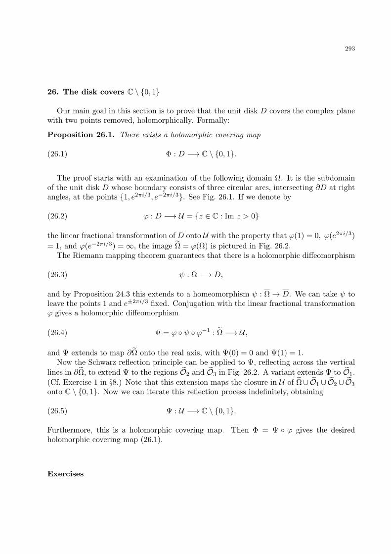
293

26. The disk covers C \ 0, 1

Our main goal in this section is to prove that the unit disk D covers the complex planewith two points removed, holomorphically. Formally:

Proposition 26.1. There exists a holomorphic covering map

(26.1) Φ : D −→ C \ 0, 1.

The proof starts with an examination of the following domain Ω. It is the subdomainof the unit disk D whose boundary consists of three circular arcs, intersecting ∂D at rightangles, at the points 1, e2πi/3, e−2πi/3. See Fig. 26.1. If we denote by

(26.2) φ : D −→ U = z ∈ C : Im z > 0

the linear fractional transformation of D onto U with the property that φ(1) = 0, φ(e2πi/3)

= 1, and φ(e−2πi/3) = ∞, the image Ω = φ(Ω) is pictured in Fig. 26.2.The Riemann mapping theorem guarantees that there is a holomorphic diffeomorphism

(26.3) ψ : Ω −→ D,

and by Proposition 24.3 this extends to a homeomorphism ψ : Ω → D. We can take ψ toleave the points 1 and e±2πi/3 fixed. Conjugation with the linear fractional transformationφ gives a holomorphic diffeomorphism

(26.4) Ψ = φ ψ φ−1 : Ω −→ U ,

and Ψ extends to map ∂Ω onto the real axis, with Ψ(0) = 0 and Ψ(1) = 1.Now the Schwarz reflection principle can be applied to Ψ, reflecting across the vertical

lines in ∂Ω, to extend Ψ to the regions O2 and O3 in Fig. 26.2. A variant extends Ψ to O1.

(Cf. Exercise 1 in §8.) Note that this extension maps the closure in U of Ω∪ O1 ∪ O2 ∪ O3

onto C \ 0, 1. Now we can iterate this reflection process indefinitely, obtaining

(26.5) Ψ : U −→ C \ 0, 1.

Furthermore, this is a holomorphic covering map. Then Φ = Ψ φ gives the desiredholomorphic covering map (26.1).

Exercises

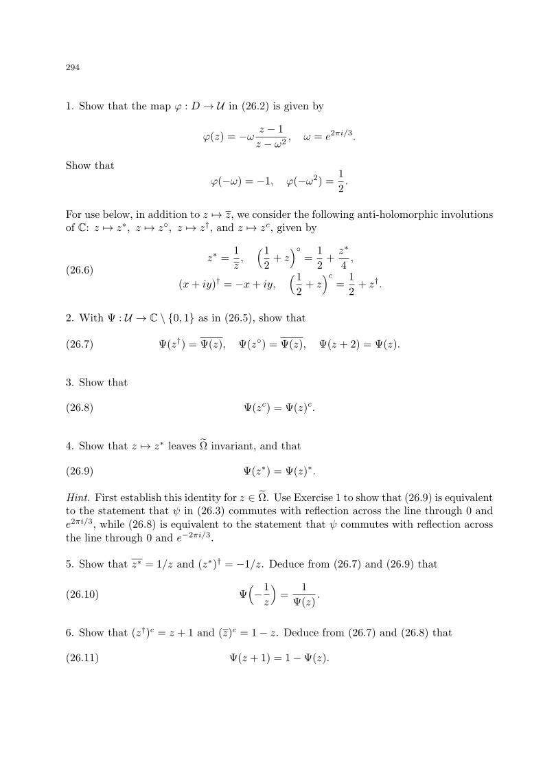
294

1. Show that the map φ : D → U in (26.2) is given by

φ(z) = −ω z − 1

z − ω2, ω = e2πi/3.

Show that

φ(−ω) = −1, φ(−ω2) =1

2.

For use below, in addition to z 7→ z, we consider the following anti-holomorphic involutionsof C: z 7→ z∗, z 7→ z, z 7→ z†, and z 7→ zc, given by

(26.6)z∗ =

1

z,

(12+ z

)=

1

2+z∗

4,

(x+ iy)† = −x+ iy,(12+ z

)c=

1

2+ z†.

2. With Ψ : U → C \ 0, 1 as in (26.5), show that

(26.7) Ψ(z†) = Ψ(z), Ψ(z) = Ψ(z), Ψ(z + 2) = Ψ(z).

3. Show that

(26.8) Ψ(zc) = Ψ(z)c.

4. Show that z 7→ z∗ leaves Ω invariant, and that

(26.9) Ψ(z∗) = Ψ(z)∗.

Hint. First establish this identity for z ∈ Ω. Use Exercise 1 to show that (26.9) is equivalentto the statement that ψ in (26.3) commutes with reflection across the line through 0 ande2πi/3, while (26.8) is equivalent to the statement that ψ commutes with reflection acrossthe line through 0 and e−2πi/3.

5. Show that z∗ = 1/z and (z∗)† = −1/z. Deduce from (26.7) and (26.9) that

(26.10) Ψ(−1

z

)=

1

Ψ(z).

6. Show that (z†)c = z + 1 and (z)c = 1− z. Deduce from (26.7) and (26.8) that

(26.11) Ψ(z + 1) = 1−Ψ(z).

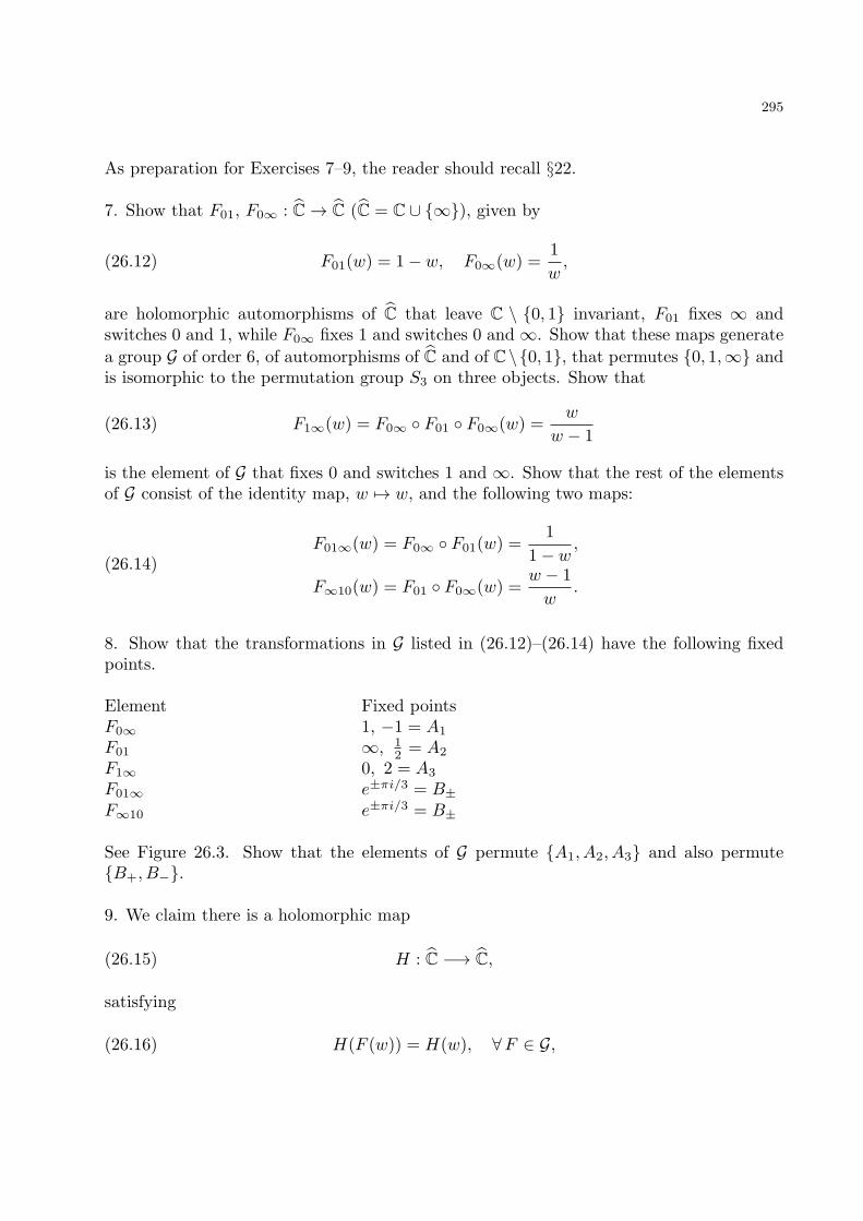
295

As preparation for Exercises 7–9, the reader should recall §22.

7. Show that F01, F0∞ : C → C (C = C ∪ ∞), given by

(26.12) F01(w) = 1− w, F0∞(w) =1

w,

are holomorphic automorphisms of C that leave C \ 0, 1 invariant, F01 fixes ∞ andswitches 0 and 1, while F0∞ fixes 1 and switches 0 and ∞. Show that these maps generate

a group G of order 6, of automorphisms of C and of C\0, 1, that permutes 0, 1,∞ andis isomorphic to the permutation group S3 on three objects. Show that

(26.13) F1∞(w) = F0∞ F01 F0∞(w) =w

w − 1

is the element of G that fixes 0 and switches 1 and ∞. Show that the rest of the elementsof G consist of the identity map, w 7→ w, and the following two maps:

(26.14)F01∞(w) = F0∞ F01(w) =

1

1− w,

F∞10(w) = F01 F0∞(w) =w − 1

w.

8. Show that the transformations in G listed in (26.12)–(26.14) have the following fixedpoints.

Element Fixed pointsF0∞ 1, −1 = A1

F01 ∞, 12 = A2

F1∞ 0, 2 = A3

F01∞ e±πi/3 = B±F∞10 e±πi/3 = B±

See Figure 26.3. Show that the elements of G permute A1, A2, A3 and also permuteB+, B−.

9. We claim there is a holomorphic map

(26.15) H : C −→ C,

satisfying

(26.16) H(F (w)) = H(w), ∀F ∈ G,

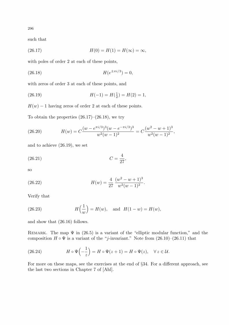
296

such that

(26.17) H(0) = H(1) = H(∞) = ∞,

with poles of order 2 at each of these points,

(26.18) H(e±πi/3) = 0,

with zeros of order 3 at each of these points, and

(26.19) H(−1) = H( 12 ) = H(2) = 1,

H(w)− 1 having zeros of order 2 at each of these points.

To obtain the properties (26.17)–(26.18), we try

(26.20) H(w) = C(w − eπi/3)3(w − e−πi/3)3

w2(w − 1)2= C

(w2 − w + 1)3

w2(w − 1)2,

and to achieve (26.19), we set

(26.21) C =4

27,

so

(26.22) H(w) =4

27

(w2 − w + 1)3

w2(w − 1)2.

Verify that

(26.23) H( 1

w

)= H(w), and H(1− w) = H(w),

and show that (26.16) follows.

Remark. The map Ψ in (26.5) is a variant of the “elliptic modular function,” and thecomposition H Ψ is a variant of the “j-invariant.” Note from (26.10)–(26.11) that

(26.24) H Ψ(−1

z

)= H Ψ(z + 1) = H Ψ(z), ∀ z ∈ U .

For more on these maps, see the exercises at the end of §34. For a different approach, seethe last two sections in Chapter 7 of [Ahl].

297

27. Montel’s theorem

Here we establish a theorem of Montel, giving a highly nontrivial and very useful suf-

ficient condition for a family of maps from a domain Ω to the Riemann sphere C to be anormal family.

Theorem 27.1. Fix a connected domain U ⊂ C and let F be the family of all holomorphic

maps f : U → C = C ∪ ∞ with range in C \ 0, 1,∞. Then F is a normal family.

Proof. There is no loss of generality in treating the case U = D, the unit disk; in particularwe can assume henceforth that U is simply connected.

Take fν ∈ F , and let K be any compact connected subset of U . We aim to show thatsome subsequence fνk converges uniformly on K. Two cases arise:

Case A. There exist pνk ∈ K such that fνk(pνk) is bounded away from 0, 1,∞ in C.

Case B. Such a subsequence does not exist.

We first take care of Case B. In fact, if Case A fails, then, given any open neighborhood

U of 0, 1,∞ in C, there exists N such that

ν ≥ N =⇒ fν(K) ⊂ U.

If U is small enough, it must have (at least) three connected components, and K connectedimplies one of them must contain fν(K) for all ν ≥ N . This readily implies that fνconverges to either 0, 1, or ∞, uniformly on K.

It remains to deal with Case A. First, to simplify the notation, relabel νk as ν. Wemake use of the holomorphic covering map Φ : D → C \ 0, 1 given in §26, and refer toFig. 26.1 in that section. Pick

ζν ∈ (Ω ∪ O1 ∪ O2 ∪ O3) ∩D

such that Φ(ζν) = f(pν). At this point it is crucial to observe that |ζν | ≤ 1 − ε for someε > 0, independent of ν. Now we take the unique lifting gν : U → D of fν such thatgν(pν) = ζν . That it is a lifting means fν = Φ gν . The existence of such a lifting followsfrom the hypothesized simple connectivity of U .

The uniform boundedness of gν implies that a subsequence (which again we relabelgν) converges locally uniformly on U ; we have gν → g : U → D. Furthermore, againpassing to a subsequence, we can assume pν → p ∈ K and

(27.1) gν(pν) = ζν → ζ ∈ D1−ε.

298

Hence g(p) = ζ ∈ D, so we actually have

(27.2) gν → g : U → D.

It follows that, for some δ > 0,

(27.3) gν(K) ⊂ D1−δ, ∀ ν.

This in turn gives the desired convergence fν → Φ g, uniformly on K.

The last argument shows that in Case A the limit function f = Φ g maps U to

C \ 0, 1,∞, so we have the following. (Compare Proposition 22.2.)

Corollary 27.2. In the setting of Theorem 27.1, if fν ∈ F and fν → f locally uniformly,then either

(27.4) f ≡ 0, f ≡ 1, f ≡ ∞, or f : U → C \ 0, 1,∞.

Exercises on Fatou sets and Julia sets

Let R : C → C be holomorphic, having the form R(z) = p(z)/q(z) with p(z) and q(z)polynomials with no common zeros. We set d = degR = max deg p,deg q, called thedegree of the map R.

1. Show that if p1 ∈ C is not a critical value of R, then R−1(p1) consists of d points.

2. Define R2 = R R, R3 = R R2, . . . , Rn = R Rn−1. Show that degRn = dn.

3. Show that if d ≥ 2 then Rn : n ≥ 1 is not a normal family of maps C → C.Hint. If Rnk is uniformly close to F : C → C, the maps must have the same degree, asshown in basic topology courses.

We say a point ζ ∈ C belongs to the Fatou set of R provided there exists a neighborhood

Ω of ζ such that Rn∣∣Ω: n ≥ 1 is a normal family, with respect to (Ω, C). The Fatou set

of R is denoted FR.

4. Show that FR is open, R : FR → FR, and Rn∣∣FR

: n ≥ 1 is normal with respect to

(FR, C).

The complement of the Fatou set is called the Julia set, JR = C \ FR. By Exercise 3,JR = ∅, whenever degR ≥ 2, which we assume from here on.

299

5. Given ζ ∈ JR, and any neighborhood O of ζ in C, consider

(27.5) EO = C \∪n≥0

Rn(O).

Use Theorem 27.1 to show that EO contains at most 2 points.

6. Set

(27.6) Eζ =∪

EO : O neighborhood of ζ.

Show that Eζ = EO for some neighborhood O of ζ. Show that R : Eζ → Eζ .

7. Consider the function Sq : C → C, given by Sq(z) = z2, Sq(∞) = ∞. Show that

(27.7) JSq = z : |z| = 1, Eζ = 0,∞, ∀ ζ ∈ JSq.

8. Suppose Eζ consists of one point. Show that R is conjugate to a polynomial, i.e., thereexists a linear fractional transformation L such that L−1RL is a polynomial.Hint. Consider the case Eζ = ∞.

9. Suppose Eζ consists of two points. Show that R is conjugate to Pm for some m ∈ Z,where Pm(z) = zm, defined appropriately at 0 and ∞.Hint. Suppose Eζ = 0,∞. Then R either fixes 0 and ∞ or interchanges them.

Conclusion. Typically, Eζ = ∅, for ζ ∈ JR. Furthermore, if Eζ = ∅, then Eζ = E isindependent of ζ ∈ JR, and E ⊂ FR.

10. Show that

(27.8) R : JR −→ JR

and

(27.9) R−1(JR) ⊂ JR.

Hint. Use Exercise 4. For (27.8), if R(ζ) ∈ FR, then ζ has a neighborhood O such thatR(O) ⊂ FR. For (27.9), use R : FR → FR.

11. Show that either JR = C or JR has empty interior.Hint. If ζ ∈ JR has a neighborhood O ⊂ JR, then, by (27.8), Rn(O) ⊂ JR. Now useExercise 5.

300

12. Show that, if p ∈ JR, then

(27.10)∪k≥0

R−k(p) is dense in JR.

Hint. Use Exercises 5–6, the “conclusion” following Exercise 9, and Exercise 10.

13. Show that

(27.11) R(z) = 1− 2

z2=⇒ JR = C.

Remark. This could be tough. See [CG], p. 82, for a proof of (27.11), using results notdeveloped in these exercises.

14. Show that

(27.12) R(z) = z2 − 2 =⇒ JR = [−2, 2] ⊂ C.

Hint. Show that R : [−2, 2] → [−2, 2], and that if z0 ∈ C \ [−2, 2], then Rk(z0) → ∞ ask → ∞.

The next exercise will exploit the following general result.

Proposition 27.3. Let X be a compact metric space, F : X → X a continuous map.Assume that for each nonempty open U ⊂ X, there exists N(U) ∈ N such that∪

0≤j≤N(U)

F j(U) = X.

Then there exists p ∈ X such that∪j≥1

F j(p) is dense in X.

15. Show that Proposition 27.3 applies to R : JR → JR.Hint. Use Exercise 5, and the conclusion after Exercise 9.

16. Show that, for R : C → C as above,

∃ p ∈ JR such that∪j≥1

Rj(p) is dense in JR.

17. Prove Proposition 27.3.

301

Hint. Take a countable dense subset qj : j ≥ 1 of X. Try to produce a shrinking familyKj ⊃ Kj+1 ⊃ · · · of nonempty, compact subsets of X, and Nj ∈ N, such that, for allj ∈ N,

FNj (Kj) ⊂ B2−j (qj).

Then take p ∈ ∩j≥1Kj , so

FNj (p) ∈ B2−j (qj), ∀ j ≥ 1.

18. Show that R : JR → JR is surjective.Hint. Consider Exercise 15.

19. Show that, for each k ∈ N, JRk = JR.Hint. Clearly FRk ⊃ FR. To get the converse, use Rj = RℓRmk, 0 ≤ ℓ ≤ k − 1.

20. Show that JR must be infinite. (Recall that we assume deg R ≥ 2.)

Hint. If JR is finite, we can replace R by Rk = R and find p ∈ JR such that R(p) = p.Then take a small neighborhood O of p (disjoint from the rest of JR) and apply Exercise

5 (and Exercise 15) to R, to get a contradiction.

21. Show that JR has no isolated points.

Hint. If p ∈ JR is isolated, let O be a small neighborhood of p in C, disjoint from the restof JR, and (again) apply Exercise 5 (and Exercise 15) to R, to get a contradiction, takinginto account Exercise 20.

These exercises provide a glimpse at an area known as Complex Dynamics. More materialon this area can be found in Chapter 5 of [Sch] (a brief treatment), and in [CG] and [Mil].As opposed to (27.7) and (27.12), typically JR has an extremely complicated, “fractal”structure, as explained in these references.

302

28. Picard’s theorems

Here we establish two theorems of E. Picard. The first, known as “Picard’s littletheorem,” is an immediate consequence of the fact that the disk holomorphically coversC \ 0, 1.

Proposition 28.1. If p and q are distinct points in C and if f : C → C \ p, q isholomorphic, then it is constant.

Proof. Without loss of generality, we can take p = 0, q = 1. Via the covering map Φ : D →C \ 0, 1 produced in §26, f lifts to a holomorphic map

(28.1) g : C −→ D, f = Φ g.

Liouville’s theorem then implies g is constant, so also f is constant.

The following sharper result is called “Picard’s big theorem.” It is proved using Montel’stheorem.

Proposition 28.2. If p and q are distinct and

(28.2) f : D \ 0 −→ C \ p, q

is holomorphic, then the singularity at 0 is either a pole or a removable singularity. Equiv-

alently, if f : D \ 0 −→ C is holomorphic and has range in C \ p, q, r with p, q, r ∈ Cdistinct, then f extends to f : D → C, holomorphic.

Proof. Again there is no loss of generality in taking p = 0, q = 1, and r = ∞. TakeΩ = D \ 0 and define fν : Ω → C \ 0, 1 by fν(z) = f(2−νz). By Montel’s theorem

(Theorem 27.1), fν is a normal family of maps from Ω to C. In particular, there existsa subsequence fνk converging locally uniformly on Ω:

(28.3) fνk → g : Ω → C,

and g is a holomorphic map. Pick r ∈ (0, 1) and set Γ = z : |z| = r ⊂ Ω. Theconvergence in (28.3) is uniform on Γ.

We consider two cases.

Case A. ∞ /∈ g(Ω).Then there exists A <∞ such that

(28.4) |fνk(z)| ≤ A, |z| = r,

for large k, or equivalently

(28.5) |f(z)| ≤ A, |z| = 2−νkr.

303

The maximum principle then implies |f(z)| ≤ A for all z close to 0, so 0 is a removablesingularity of f .

Case B. ∞ ∈ g(Ω).By Corollary 27.2, g ≡ ∞ on Ω. Consequently, 1/fνk → 0 uniformly on Γ, and thenanalogues of (28.4)–(28.5) hold with f replaced by 1/f (recall that f is nowhere vanishingon D \ 0), so f has a pole at 0.

Exercises

1. Fix distinct points a, b ∈ C, let γ be the line segment joining a and b, and assumef : C → C \ γ is holomorphic. Show that f is constant. Show this in an elementaryfashion, not using Picard theorems.

2. Suppose f : C → C is a holomorphic function that is not a polynomial. (We say fis transcendental.) Show that for every w ∈ C, with at most one exception, there areinfinitely many zν ∈ C such that f(zν) = w.

3. Test the conclusion in Exercise 2 for the function f(z) = ez.

4. Show that iff(z) = zez,

then f : C → C is onto. Relate this to Exercise 2.Hint. If f(z) is never equal to w, then

zez − w = eg(z).

What can g(z) be?

5. Suppose that f is meromorphic on C, and not constant.. Show that f can omit at mosttwo complex values. Give an example where such an omission occurs.

304

29. Harmonic functions II

Here we study further properties of harmonic functions. A key tool will be the explicitformula for the solution to the Dirichlet problem

(29.1) ∆u = 0 on D1(0), u∣∣S1 = f,

given in §13, namely

(29.2) u(z) =

∫ 2π

0

p(z, θ)f(θ) dθ,

where

(29.3) p(z, θ) =1

2π

1− |z|2

|w − z|2, w = eiθ,

as in (13.76), or equivalently (cf. (13.85))

(29.4) p(z, θ) =1

2πRe

eiθ + z

eiθ − z=

1

πRe

eiθ

eiθ − z− 1

2π.

We restrict attention to harmonic functions on domains in C = R2. However we pointout that results presented here can be extended to treat harmonic functions on domainsin Rn. In such a case we replace (29.2)–(29.3) by

(29.5) u(x) =

∫Sn−1

p(x, ω)f(ω) dS(ω),

for x ∈ B1(0) = x ∈ Rn : |x| < 1, with

(29.6) p(x, ω) =1

An−1

1− |x|2

|x− ω|n,

where An−1 is the (n − 1)-dimensional area of the unit sphere Sn−1 ⊂ Rn. A proof of(29.5)–(29.6) can be found in Chapter 5 of [T2]. But here we will say no more about thehigher-dimensional case.

We use (29.2)–(29.3) to establish a Harnack estimate, concerning the set of harmonicfunctions

(29.7) A = u ∈ C2(D) ∩ C(D) : ∆u = 0, u ≥ 0 on D, u(0) = 1,

where D = D1(0) = z ∈ C : |z| < 1.

305

Proposition 29.1. For z ∈ D,

(29.8) u ∈ A =⇒ u(z) ≥ 1− |z|1 + |z|

.

Proof. The mean value property of harmonic functions implies that f = u|∂D satisfies

(29.9)1

2π

∫ 2π

0

f(θ) dθ = 1,

if u ∈ A. Given this, (29.8) follows from (29.2)–(29.3) together with the estimate

(29.10)1− |z|2

|w − z|2≥ 1− |z|

1 + |z|, for |z| < 1, |w| = 1.

To get (29.10), note that if w = eiφ, z = reiθ, and ψ = φ− θ, then

(29.11)

|w − z|2 = (eiψ − r)(e−iψ − r)

= 1− 2r cosψ + r2

≤ 1 + 2r + r2 = (1 + r)2,

from which (29.10) follows.

By translating and scaling, we deduce that if u is ≥ 0 and harmonic on DR(p), then

(29.12) |z − p| = a ∈ [0, R) =⇒ u(z) ≥ R− a

R+ au(p).

This leads to the following extension of the Liouville theorem, Proposition 7.5 (with adifferent approach from that suggested in Exercise 1 of §7).

Proposition 29.2. If u is harmonic on all of C (and real valued) and bounded from below,then u is constant.

Proof. Adding a constant if necessary, we can assume u ≥ 0 on C. Pick z0, z1 ∈ C andset a = |z0 − z1|. By (29.12),

(29.13) u(z0) ≥R− a

R+ au(z1), ∀R ∈ (a,∞),

hence, taking R→ ∞,

(29.14) u(z0) ≥ u(z1),

for all z0, z1 ∈ C. Reversing roles gives

(29.15) u(z0) = u(z1),

and proves the proposition.

The following result will lead to further extensions of Liouville’s theorem.

306

Proposition 29.3. There exists a number A ∈ (0,∞) with the following property. Let ube harmonic in DR(0). Assume

(29.16) u(0) = 0, u(z) ≤M on DR(0).

Then

(29.17) u(z) ≥ −AM on DR/2(0).

Proof. Set v(z) =M − u(z), so v ≥ 0 on DR(0) and v(0) =M . Take

(29.18) p ∈ DR/2(0), u(p) = infDR/2(0)

u.

From (29.12), with R replaced by R/2, a by R/4, and u by v, we get

(29.19) v(z) ≥ 1

3

(M − u(p)

)on DR/2(p).

Hence

(29.20)1

Area DR(0)

∫∫DR(0)

v(z) dx dy ≥ 1

16· 13

(M − u(p)

).

On the other hand, the mean value property for harmonic functions implies that the leftside of (29.20) equals v(0) =M , so we get

(29.21) M − u(p) ≤ 48M,

which implies (29.17).

Note that Proposition 29.3 gives a second proof of Proposition 29.2. Namely, underthe hypotheses of Proposition 29.2, if we set v(z) = u(0) − u(z), we have v(0) = 0 andv(z) ≤ u(0) on C (if u ≥ 0 on C), hence, by Proposition 29.3, v(z) ≥ −Au(0) on C, so vis bounded on C, and Proposition 7.5 implies v is constant. Note however, that the firstproof of Proposition 29.2 did not depend upon Proposition 7.5.

Here is another corollary of Proposition 29.3.

Proposition 29.4. Assume u is harmonic on C and there exist C0, C1 ∈ (0,∞), andk ∈ Z+ such that

(29.22) u(z) ≤ C0 + C1|z|k, ∀ z ∈ C.

Then there exist C2, C3 ∈ (0,∞) such that

(29.23) u(z) ≥ −C2 − C3|z|k, ∀ z ∈ C.

307

Proof. Apply Proposition 29.3 to u(z)− u(0), M = C0 + |u(0)|+ C1Rk.

Note that as long as C2 ≥ C0 and C3 ≥ C1, the two one-sided bounds (29.22) and(29.23) imply

(29.24) |u(z)| ≤ C2 + C3|z|k, ∀ z ∈ C.

We aim to show that if u(z) is harmonic on C and satisfies the bound (29.24), then umust be a polynomial in x and y. For this, it is useful to have estimates on derivatives∂ix∂

jyu, which we turn to.

If u ∈ C2(D) ∩ C(D) is harmonic on D = D1(0), the formula (25.2) yields

(29.25) ∂ix∂jyu(z) =

∫ 2π

0

pij(z, θ)f(θ) dθ,

where

(29.26) pij(z, θ) = ∂ix∂jyp(z, θ).

From (29.3) it is apparent that p(z, θ) is smooth in z ∈ D. We have bounds of the form

(29.27) |pij(z, θ)| ≤ Kij , |z| ≤ 1

2.

For example, from (29.4) we get

(29.28)

∂

∂xp(z, θ) =

1

πRe

eiθ

(eiθ − z)2,

∂

∂yp(z, θ) =

1

πRe

ieiθ

(eiθ − z)2.

Hence

(29.29)

|∇x,yp(z, θ)| ≤1

π

1

|eiθ − z|2

≤ 1

π(1− |z|)2,

the last estimate by a variant of (29.11).Applied to (29.25), the bounds (29.27) imply

(29.30) sup|z|≤1/2

|∂ix∂jyu(z)| ≤ 2πKij supD

|u(z)|,

whenever u ∈ C2(D) ∩ C(D) is harmonic on D.We are now are ready for the following.

308

Proposition 29.5. If u : C → R is harmonic and, for some k ∈ Z+, Cj ∈ (0,∞),

(29.31) u(z) ≤ C0 + C1|z|k, ∀ z ∈ C,

then u is a polynomial in x and y of degree k.

Proof. By Proposition 29.4, we have the two-sided bound

(29.32) |u(z)| ≤ C2 + C3|z|k, ∀ z ∈ C.

Now set vR(z) = R−ku(Rz). We have vR|D bounded, independent of R ∈ [1,∞), whereD = D1(0). Hence, by (29.30), ∂ix∂

jyvR is bounded on D1/2(0), independent of R, for each

i, j ∈ Z+, so

(29.33) Ri+j−k|∂ix∂jyu(Rz)| ≤ Cij , |z| ≤ 1

2, R ∈ [1,∞).

Taking R→ ∞ yields ∂ix∂jyu = 0 on C for i+ j > k, which proves the proposition.

Remark. In case k = 0, the argument above gives another proof of Proposition 7.5.

Recall from §7 the mean value property satisfied by a harmonic function u ∈ C2(Ω),

namely, if Dr(z0) ⊂ Ω, then

(29.34) u(z0) =1

πr2

∫∫Dr(z0)

u(x, y) dx dy,

a result mentioned above in connection with (29.20). We now establish the followingconverse.

Proposition 29.6. Let Ω ⊂ C be open and let u : Ω → R be continuous and satisfy themean value property (29.34) whenever Dr(z0) ⊂ Ω. Then u is harmonic on Ω.

Proof. It suffices to prove that u is harmonic on Dρ(z1) whenever Dρ(z1) ⊂ Ω. To see this,

let f = u|∂Dρ(z1), and let v ∈ C2(Dρ(z1)) ∩ C(Dρ(z1)) solve the Dirichlet problem

(29.35) ∆v = 0 on Dρ(z1), v∣∣∂Dρ(z1)

= f.

The function v is given by a construction parallel to that for (29.1). It then suffices toshow that

(29.36) v = u on Dρ(z1).

To see this, consider w = v − u ∈ C(Dρ(z1)), which satisfies

(29.37) w∣∣∂Dρ(z1)

= 0,

309

and

(29.38) w(z2) =1

πr2

∫∫Dr(z2)

w(x, y) dx dy, whenever Dr(z2) ⊂ Dρ(z1).

Now, argunig as in the proof of Proposition 7.4 (cf. also Proposition 6.1), we see that

(29.39) supDρ(z1)

|w| = sup∂Dρ(z1)

|w|,

and hence, by (29.37), w ≡ 0 on Dρ(z1). This gives (29.36) and finishes the proof ofProposition 29.6.

We next use the solvability of the Dirichlet problem (29.1) to establish the followingremovable singularity theorem, which extends the scope of Theorem 11.1.

Proposition 29.7. Let Ω ⊂ C be open, p ∈ Ω, and u ∈ C2(Ω \ p) be harmonic. If u isbounded, then there is a harmonic u ∈ C2(Ω) such that u = u on Ω \ p.

Proof. It suffices to assume that p = 0, D1(0) ⊂ Ω, and that u is real valued. Say |u| ≤M

on D∗1 = D1(0) \ 0. Take v ∈ C2(D1(0)) ∩ C(D1(0)) to satisfy

(29.40) ∆v = 0 on D1(0), v∣∣S1 = u

∣∣S1 ,

so w = u− v is C2 on D1(0) \ 0, continuous on D1(0) \ 0, and satisfies

(29.41) ∆w = 0 on D1(0) \ 0, w∣∣S1 = 0.

Also, the maximum principle applied to (29.40) yields |v| ≤ M , hence |w| ≤ 2M , on D∗1 .

If we restrict w to z ∈ C : a ≤ |z| ≤ 1 and compare with

(29.42) ψ(z) =(log

1

a

)−1

log1

|z|,

which is harmonic on z = 0, and vanishes at |z| = 1, the maximum principle implies

(29.43) |w(z)| ≤ 2M(log

1

a

)−1

log1

|z|, for a ≤ |z| ≤ 1,

whenever a ∈ (0, 1). Letting a 0 yields w ≡ 0 on 0 < |z| ≤ 1, hence

(29.44) u(z) = v(z) for 0 < |z| ≤ 1.

Thus we can set u = u on Ω \ 0 and u = v on D1(0), to complete the proof of Proposition29.7.

310

We turn now to the Dirichlet problem on more general domains, that is, to the problemof finding u ∈ C2(Ω) ∩ C(Ω) satisfying

(29.45) ∆u = 0 on Ω, u∣∣∂Ω

= φ,

given φ ∈ C(∂Ω), given Ω ⊂ C a bounded open set. It is a consequence of the maximumprinciple, which implies that

(29.46) supΩ

|u| = sup∂Ω

|u|,

that such a solution, if it exists, is unique. We focus on those bounded, simply connecteddomains Ω such that the Riemann mapping function

(29.47) f : D −→ Ω

extends to a homeomorphism f : D → Ω, with inverse

(29.48) g : Ω −→ D,

holomorphic on Ω. Here, D = D1(0) is the unit disk. A class of domains satisfying thiscondition is given in Proposition 24.3. In such a case, by Proposition 7.9, we have

(29.49) u(z) = v(g(z)),

where v ∈ C2(D) ∩ C(D) satisfies

(29.50) ∆v = 0 on D, v∣∣∂D

= ψ = φ f.

From (29.2), we have

(29.51) v(z) =

∫ 2π

0

p(z, θ)ψ(eiθ) dθ,

with p(z, θ) given by (29.3)–(29.4). We have the following conclusion.

Proposition 29.8. Assume Ω ⊂ C is a bounded, simply connected domain with the prop-erty that the Riemann mapping function f : D → Ω extends to a homeomorphism from Dto Ω, with inverse g, as in (29.48). Then given φ ∈ C(∂Ω), the Dirichlet problem (29.45)has a unique solution u ∈ C2(Ω) ∩ C(Ω), given by

(29.52)

u(z) =

∫ 2π

0

p(g(z), θ)φ(f(eiθ)) dθ

=1

2π

∫ π

−π

1− |g(z)|2

|eiθ − g(z)|2φ(f(eiθ)) dθ.

311

We examine how this works out when Ω = H+ is the upper half plane

(29.53) H+ = z ∈ C : Im z > 0,

for which (29.47)–(29.48) hold with

(29.54) g(z) =i− z

i+ z, f(z) = i

1− z

1 + z.

This is slightly outside the results of (29.47)–(29.48) since H+ is not bounded, but itworks if we regard H+ as a relatively compact subset of the Riemann sphere C ∪ ∞,with boundary ∂H+ = R ∪ ∞. In this case, we have

(29.55) t = f(eiθ) = i1− eiθ

1 + eiθ= tan

θ

2,

for which dθ = 2 dt/(1 + t2), and (29.52) yields

(29.56) u(z) =1

π

∫ ∞

−∞

1− |g(z)|2

|g(t)− g(z)|2φ(t)

dt

1 + t2.

For g(z) as in (29.54), we calculate that

(29.57)1− |g(z)|2

|g(t)− g(z)|2=

y(1 + t2)

(x− t)2 + y2, z = x+ iy ∈ H+,

so we obtain the formula

(29.58) u(z) =1

π

∫ ∞

−∞

y

(x− t)2 + y2φ(t) dt,

for the solution to (29.45) with Ω = H+. Note that we are assuming that φ : R∪∞ → Cis continuous.

It is of interest to consider an alternative derivation of (29.58), using the Fourier trans-form, introduced in §14. Namely, consider

(29.59) u(x, y) =1√2π

∫ ∞

−∞e−y|ξ|φ(ξ)eixξ dξ,

with φ ∈ A(R), defined in (14.21). We have, for y > 0,

(29.60)

∂2

∂y2u(x, y) =

1√2π

∫ ∞

−∞e−y|ξ|ξ2φ(ξ)eixξ dξ

= − ∂2

∂x2u(x, y).

312

Hence u(x, y) solves

(29.61) ∆u = 0 on H+, u(x, 0) = φ(x).

Furthermore, substituting the definition of φ(ξ) into (29.59) yields

(29.62) u(x, y) =1

2π

∫ ∞

−∞

∫ ∞

−∞e−y|ξ|+i(x−t)ξφ(t) dξ dt,

and a computation of the integral

(29.63)

∫ ∞

−∞e−y|ξ|+i(x−t)ξ dξ

(cf. Exercise 4 of §14), yields (29.58).Let us note that direct applications of (29.58) and (29.59) yield, respectively,

(29.64) |u(x, y)| ≤ supt

|φ(t)|, |u(x, y)| ≤ (2π)−1/2∥φ∥L1 ,

for all x ∈ R, y > 0. Also, from both (29.58) and (29.59), it follows that

(29.65) supx∈R

|u(x, y)− φ(x)| −→ 0, as y 0,

via (29.58) for φ ∈ C(R) vanishing at ∞, and, via (29.59), for φ ∈ A(R). In light of theseresults, the following uniqueness result is of interest.

Proposition 29.9. Let u ∈ C2(H+) ∩ C(H+) satisfy ∆u = 0 on H+ and u(x, 0) = 0.Assume |u(x, y)| ≤M <∞ on H+. Then u ≡ 0.

Proof. For x ∈ R, set

(29.66)v(x, y) = u(x, y), y ≥ 0,

− u(x,−y), y < 0.

Then, by Proposition 13.8, v is harmonic on C. Also |v(x, y)| ≤ M for all (x, y) ∈ R2.It follows from Liouville’s theorem, Proposition 7.5, that u is constant. Of course, theconstant must be 0.

We next look at the Dirichlet problem (29.45) when

(29.67) Ω = D+ = z ∈ C : |z| < 1 and Im z > 0.

In this case, a construction of a conformal map g : Ω → D is indicated in Fig. 22.1. Usingthis, we could implement (29.49). Rather than recording further details of that approach,we now describe another way to solve

(29.68) ∆u = 0 on D+, u = φ on ∂D+ = [−1, 1] ∪ S+,

313

where S+ = eis : 0 ≤ s ≤ π, which will involve breaking φ into pieces. First, subtractinga harmonic function of the form a + bx, we can reduce our problem to the case whereφ(−1) = φ(1) = 0. Then write φ = φ0 + φ1, where φj ∈ C(∂D+), with φ0 supported on[−1, 1] and φ1 supported on S+. We define φ0 on all of R to be 0 on R \ [−1, 1], and letu0 solve

(29.69) ∆u0 = 0 on H+, u0(x, 0) = φ0(x),

as in (29.61). The solution is given by (29.58), with φ(t) replaced by φ0(t). We then seethat the solution to (29.68) is given by u = u0 + u1, where

(29.70) ∆u1 = 0 on D+, u1∣∣∂D+ = ψ0 = φ− u0

∣∣∂D+ .

Note that ψ0 ∈ C(∂D+) is supported on S+. We can now define ψ ∈ C(S1) by

(29.71)ψ(x, y) = ψ0(x, y), (x, y) ∈ S+,

− ψ0(x,−y), (x,−y) ∈ S+,

and obtain u1 as the restriction to D+ of v, solving

(29.72) ∆v = 0 on D1(0), v∣∣S1 = ψ.

Note that v(x,−y) = −v(x, y).We move on to a consideration of the Dirichlet problem on an “exterior domain.” Let

U ⊂ C be a bounded open set, and let Ω = C\U . We seek a solution u ∈ C2(Ω)∩C(Ω) to

(29.73) ∆u = 0 on Ω, u∣∣∂Ω

= f,

given f ∈ C(∂Ω). We also impose the condition that

(29.74) u is bounded on Ω.

To get this, we take z0 ∈ U and set

(29.75) u(z) = v( 1

z − z0

), i.e., v(ζ) = u

(1ζ+ z0

),

where

(29.76) ∆v(ζ) = 0 for ζ−1 + z0 ∈ Ω.

Note that

(29.77) ζ ∈ C \ 0 : ζ−1 + z0 ∈ Ω = Ω∗ \ 0,

314

where Ω∗ is the image of Ω ∪ ∞ ⊂ C ∪ ∞ under the map z 7→ 1/(z − z0). Thusa bounded harmonic function u on Ω corresponds to a bounded harmonic function v onΩ∗ \ 0. Proposition 29.7 implies that such v must extend to be harmonic on Ω∗. Thus(29.73)–(29.74) translates to the Dirichlet problem

(29.78) ∆v = 0 on Ω∗, v∣∣∂Ω∗ = g,

where

(29.79) g(ζ) = f(ζ−1 + z0), ζ ∈ ∂Ω∗.

One simple case of (29.73)–(29.79) arises from

(29.80) Ω = C \D1(0), with Ω∗ = D1(0).

A more elaborate case is

(29.81) Ω = C \D1(−a) ∪D1(a)

,

given a > 1, mentioned in the exercises below.To close, we mention that the Dirichlet problem (29.45), for a general bounded open

donain Ω ⊂ C, is not always solvable for u ∈ C(Ω), given arbitrary φ ∈ C(∂Ω). Forexample, let

(29.82) Ω = z ∈ C : 0 < |z| < 1, ∂Ω = S1 ∪ 0,

and take φ ∈ C(S1 ∪ 0). By Proposition 29.7, the solution u is uniquely determinedby u|S1 alone. If this solution does not agree with φ(0) at z = 0, then, strictly speaking,we do not have (29.45). We say 0 is an irregular boundary point for Ω in (29.82). It is ofinterest to characterize domains without irregular boundary points. Furthermore, there isa notion of a generalized solution to (29.45) in the presence of irregular boundary points.Material on this, both for planar domains and higher dimensional domains, can be foundin Chapter 5 of [T2].

In addition, results in §§4–6 of that Chapter 5 allow for a proof of the Riemann map-ping theorem, as a consequence of solving the Dirichlet problem, thus going in the oppositedirection from Proposition 29.8 of this section. As an alternative to presenting that argu-ment, we will show how solving a Dirichlet problem on another class of domains gives riseto a variant of the Riemann mapping theorem.

Namely, suppose Ω ⊂ C is a smoothly bounded domain whose boundary consists of twosmooth, simple closed curves, say γ0 and γ1. Let u be the solution to the Dirichlet problem

(29.83) ∆u = 0 on Ω, u∣∣γ0

= 0, u∣∣γ1

= −1.

If ∂Ω is C∞, then u ∈ C∞(Ω). We know from Proposition 7.4 that −1 < u < 0 on Ω. Inaddition, a “strong maximum principle” (cf. Chapter 5, §2 of [T2]) implies

(29.84)∂u

∂ν> 0 on γ0,

∂u

∂ν< 0 on γ1,

315

where ν is the unit outward normal to ∂Ω. We set

(29.85) G = cu,

where c is a positive constant to be determined, and, following (7.22), try to produce aharmonic conjugate to G, of the form

(29.86) H(z) =

∫γαz

(−∂G∂y

dx+∂G

∂xdy

),

where we pick α ∈ Ω and then γαz is a smooth path from α to z. By Lemma 7.7, if γαzand γαz are homotopic paths from α to z, the integrals coincide. However, in this case Ωis not simply connected, and (27.86) does not yield a single-valued harmonic conjugate ofG. Here is what we get instead. We have

(29.87)

∫γ0

(−∂G∂y

dx+∂G

∂xdy

)=

∫γ0

∂G

∂νds

= c

∫γ0

∂u

∂νds

> 0.

Hence there is a unique value of c ∈ (0,∞) such that (29.87) is equal to 2π. For such c,the function H in (29.86) is well defined, up to an additive integral multiple of 2π. Hence

(29.88) Ψ = eG+iH

is a single-valued, holomorphic function on Ω, extending smoothly to Ω. It maps γ0 toC0 = z ∈ C : |z| = 1, and it maps γ1 to C1 = z ∈ C : |z| = e−c. Consequently,

(29.89) Ψ : Ω −→ Aρ = z ∈ C : ρ < |z| < 1, ρ = e−c,

extending smoothly to Ψ : Ω → Aρ. It follows from (29.84) and the Cauchy-Riemannequations that the tangential derivative of H is never vanishing on ∂Ω, hence

(29.90)ψj = Ψ

∣∣γj, ψj : γj → Cj

⇒ ψ′j is nowhere vanishing on γj .

In fact |ψ′j(z)| = |∂νG(z)| for z ∈ γj . Thus the choice of c yields

(29.91)

∫γ0

|ψ′0(z)| · |dz| = 2π,

so ψ0 : γ0 → C0 is a diffeomorphism.Now if we pick w ∈ Aρ, we see that ψ0 : γ0 → C0 has winding number 1 about w. We

can apply the argument principle (Proposition 17.5), to deduce that there is a unique z ∈ Ωsuch that Ψ(z) = w. We have the following variant of the Riemann mapping theorem forannular regions.

316

Proposition 29.10. If Ω ⊂ C is a smoothly bounded domain with two boundary compo-nents, and Ψ is constructed as in (29.83)–(29.89), then Ψ is a holomorphic diffeomorphismfrom Ω onto Aρ, extending to a smooth diffeomorphism from Ω onto Aρ

We note that if 0 < ρ < σ < 1, then Aρ and Aσ are not holomorphically equivalent.Indeed, if there were a holomorphic diffeomorphism F : Aρ → Aσ, then, using an inversionif necessary, we could assume F maps |z| = 1 to itself and maps |z| = ρ to |z| = σ.Then, applying the Schwarz reflection principle an infinite number of times, we can extendF to a holomorphic diffeomorphism of D1(0) = |z| ≤ 1 onto itself, preserving the origin.Then we must have F (z) = az, |a| = 1, which would imply ρ = σ.

Exercises

1. Suppose f : C → C is holomorphic and |f(z)| ≤ AeB|z|. Show that if f has only finitelymany zeros then f has the form

f(z) = p(z) eaz+b,

for some polynomial p(z).Hint. If p(z) has the same zeros as f(z), write f(z)/p(z) = eg(z) and apply Proposition29.5 to Re g(z).

2. Show that the function ez − z (considered in Exercise 10 of §6) has infinitely manyzeros. More generally, show that, for each a ∈ C, ez − z − a has infinitely many zeros.

3. The proof given above of Proposition 29.3 shows that (29.17) holds with A = 47. Canyou show it holds with some smaller A?

4. Given ρ ∈ (0, 1), consider the annulus Aρ = z ∈ C : ρ < |z| < 1, and the Dirichletproblem

(29.92) ∆u = 0 on Aρ, u(eiθ) = f(θ), u(ρeiθ) = g(θ).

Produce the solution in the form

u(reiθ) =∑k∈Z\0

(akrk + bkr

−k)eikθ + a0 + b0 log r.

Solve for ak and bk in terms of f(k) and g(k). Show that, if f, g ∈ A(S1), defined in (13.28),then this series converges absolutely and uniformly on Aρ to the solution to (29.92).

5. Consider Ω = C \ D1(−a)∪D1(a), with a > 1, as in (29.81). Find a linear fractionaltransformation mapping Ω∪ ∞ conformally onto an annulus Aρ, given as in Exercise 4.Use this to analyze the Dirichlet problem (29.73)–(29.74), in this setting.

317

D. Surfaces and metric tensors

A smooth m-dimensional surface M ⊂ Rn is characterized by the following property.Given p ∈M, there is a neighborhood U of p in M and a smooth map φ : O → U, from anopen set O ⊂ Rm bijectively to U, with injective derivative at each point, and continuousinverse φ−1 : U → O. Such a map φ is called a coordinate chart on M. We call U ⊂ Ma coordinate patch. If all such maps φ are smooth of class Ck, we say M is a surface ofclass Ck.

There is an abstraction of the notion of a surface, namely the notion of a “manifold,”which we discuss later in this appendix.

If φ : O → U is a Ck coordinate chart, such as described above, and φ(x0) = p, we set

(D.1) TpM = RangeDφ(x0),

a linear subspace of Rn of dimensionm, and we denote byNpM its orthogonal complement.It is useful to consider the following map. Pick a linear isomorphism A : Rn−m → NpM ,and define

(D.2) Φ : O × Rn−m −→ Rn, Φ(x, z) = φ(x) +Az.

Thus Φ is a Ck map defined on an open subset of Rn. Note that

(D.3) DΦ(x0, 0)

(vw

)= Dφ(x0)v +Aw,

so DΦ(x0, 0) : Rn → Rn is surjective, hence bijective, so the Inverse Function Theoremapplies; Φ maps some neighborhood of (x0, 0) diffeomorphically onto a neighborhood ofp ∈ Rn.

Suppose there is another Ck coordinate chart, ψ : Ω → U . Since φ and ψ are byhypothesis one-to-one and onto, it follows that F = ψ−1 φ : O → Ω is a well defined map,which is one-to-one and onto. See Fig. D.1. Also F and F−1 are continuous. In fact, wecan say more.

Lemma D.1. Under the hypotheses above, F is a Ck diffeomorphism.

Proof. It suffices to show that F and F−1 are Ck on a neighborhood of x0 and y0, re-spectively, where φ(x0) = ψ(y0) = p. Let us define a map Ψ in a fashion similar to (5.2).

To be precise, we set TpM = RangeDψ(y0), and let NpM be its orthogonal complement.

(Shortly we will show that TpM = TpM , but we are not quite ready for that.) Then pick a

linear isomorphism B : Rn−m → NpM and set Ψ(y, z) = ψ(y)+Bz, for (y, z) ∈ Ω×Rn−m.Again, Ψ is a Ck diffeomorphism from a neighborhood of (y0, 0) onto a neighborhood of p.

318

To be precise, there exist neighborhoods O of (x0, 0) in O × Rn−m, Ω of (y0, 0) in

Ω× Rn−m, and U of p in Rn such that

Φ : O −→ U , and Ψ : Ω −→ U

are Ck diffeomorphisms. It follows that Ψ−1 Φ : O → Ω is a Ck diffeomorphism. Now

note that, for (x0, 0) ∈ O and (y, 0) ∈ Ω,

(D.4) Ψ−1 Φ(x, 0) =(F (x), 0

), Φ−1 Ψ(y, 0) =

(F−1(y), 0

).

In fact, to verify the first identity in (D.4), we check that

Ψ(F (x), 0) = ψ(F (x)) +B0

= ψ(ψ−1 φ(x))= φ(x)

= Φ(x, 0).

The identities in (D.4) imply that F and F−1 have the desired regularity.

Thus, when there are two such coordinate charts, φ : O → U, ψ : Ω → U , we have aCk diffeomorphism F : O → Ω such that

(D.5) φ = ψ F.

By the chain rule,

(D.6) Dφ(x) = Dψ(y)DF (x), y = F (x).

In particular this implies that RangeDφ(x0) = RangeDψ(y0), so TpM in (D.1) is inde-pendent of the choice of coordinate chart. It is called the tangent space to M at p.

We next define an object called the metric tensor on M . Given a coordinate chartφ : O → U , there is associated an m × m matrix G(x) =

(gjk(x)

)of functions on O,

defined in terms of the inner product of vectors tangent to M :

(D.7) gjk(x) = Dφ(x)ej ·Dφ(x)ek =∂φ

∂xj· ∂φ∂xk

=

n∑ℓ=1

∂φℓ∂xj

∂φℓ∂xk

,

where ej : 1 ≤ j ≤ m is the standard orthonormal basis of Rm. Equivalently,

(D.8) G(x) = Dφ(x)tDφ(x).

We call (gjk) the metric tensor ofM, on U , with respect to the coordinate chart φ : O → U .Note that this matrix is positive-definite. From a coordinate-independent point of view,

319

the metric tensor on M specifies inner products of vectors tangent to M , using the innerproduct of Rn.

If we take another coordinate chart ψ : Ω → U, we want to compare (gjk) with H =(hjk), given by

(D.9) hjk(y) = Dψ(y)ej ·Dψ(y)ek, i.e., H(y) = Dψ(y)t Dψ(y).

As seen above we have a diffeomorphism F : O → Ω such that (5.5)–(5.6) hold. Conse-quently,

(D.10) G(x) = DF (x)tH(y)DF (x),

or equivalently,

(D.11) gjk(x) =∑i,ℓ

∂Fi∂xj

∂Fℓ∂xk

hiℓ(y).

We now define the notion of surface integral on M . If f : M → R is a continuousfunction supported on U, we set

(D.12)

∫M

f dS =

∫O

f φ(x)√g(x) dx,

where

(D.13) g(x) = detG(x).

We need to know that this is independent of the choice of coordinate chart φ : O → U. Thus,if we use ψ : Ω → U instead, we want to show that (D.12) is equal to

∫Ωf ψ(y)

√h(y) dy,

where h(y) = detH(y). Indeed, since f ψ F = f φ, we can apply the change of variableformula for multidimensional integrals, to get

(D.14)

∫Ω

f ψ(y)√h(y) dy =

∫O

f φ(x)√h(F (x)) |det DF (x)| dx.

Now, (D.10) implies that

(D.15)√g(x) = |det DF (x)|

√h(y),

so the right side of (D.14) is seen to be equal to (D.12), and our surface integral is welldefined, at least for f supported in a coordinate patch. More generally, if f :M → R hascompact support, write it as a finite sum of terms, each supported on a coordinate patch,and use (D.12) on each patch.

320

Let us pause to consider the special cases m = 1 and m = 2. For m = 1, we areconsidering a curve in Rn, say φ : [a, b] → Rn. Then G(x) is a 1 × 1 matrix, namelyG(x) = |φ′(x)|2. If we denote the curve in Rn by γ, rather than M, the formula (D.12)becomes

(D.16)

∫γ

f ds =

∫ b

a

f φ(x) |φ′(x)| dx.

In case m = 2, let us consider a surface M ⊂ R3, with a coordinate chart φ : O → U ⊂M.For f supported in U, an alternative way to write the surface integral is

(D.17)

∫M

f dS =

∫O

f φ(x) |∂1φ× ∂2φ| dx1dx2,

where u × v is the cross product of vectors u and v in R3. To see this, we compare thisintegrand with the one in (D.12). In this case,

(D.18) g = det

(∂1φ · ∂1φ ∂1φ · ∂2φ∂2φ · ∂1φ ∂2φ · ∂2φ

)= |∂1φ|2|∂2φ|2 − (∂1φ · ∂2φ)2.

Recall that |u × v| = |u| |v| | sin θ|, where θ is the angle between u and v. Equivalently,since u · v = |u| |v| cos θ,

(D.19) |u× v|2 = |u|2|v|2(1− cos2 θ

)= |u|2|v|2 − (u · v)2.

Thus we see that |∂1φ× ∂2φ| =√g, in this case, and (D.17) is equivalent to (D.12).

An important class of surfaces is the class of graphs of smooth functions. Let u ∈ C1(Ω),for an open Ω ⊂ Rn−1, and let M be the graph of z = u(x). The map φ(x) =

(x, u(u)

)provides a natural coordinate system, in which the metric tensor is given by

(D.20) gjk(x) = δjk +∂u

∂xj

∂u

∂xk.

If u is C1, we see that gjk is continuous. To calculate g = det(gjk), at a given point p ∈ Ω,if ∇u(p) = 0, rotate coordinates so that ∇u(p) is parallel to the x1 axis. We see that

(D.21)√g =

(1 + |∇u|2

)1/2.

In particular, the (n− 1)-dimensional volume of the surface M is given by

(D.22) Vn−1(M) =

∫M

dS =

∫Ω

(1 + |∇u(x)|2

)1/2dx.

321

Particularly important examples of surfaces are the unit spheres Sn−1 in Rn,

(D.23) Sn−1 = x ∈ Rn : |x| = 1.

Spherical polar coordinates on Rn are defined in terms of a smooth diffeomorphism

(D.24) R : (0,∞)× Sn−1 −→ Rn \ 0, R(r, ω) = rω.

Let (hℓm) denote the metric tensor on Sn−1 (induced from its inclusion in Rn) with respectto some coordinate chart φ : O → U ⊂ Sn−1. Then, with respect to the coordinate chartΦ : (0,∞) × O → U ⊂ Rn given by Φ(r, y) = rφ(y), the Euclidean metric tensor can bewritten

(D.25)(ejk

)=

(1

r2hℓm

).

To see that the blank terms vanish, i.e., ∂rΦ · ∂xjΦ = 0, note that φ(x) · φ(x) = 1 ⇒∂xjφ(x) · φ(x) = 0. Now (D.25) yields

(D.26)√e = rn−1

√h.

We therefore have the following result for integrating a function in spherical polar coordi-nates.

(D.27)

∫Rn

f(x) dx =

∫Sn−1

[∫ ∞

0

f(rω)rn−1 dr]dS(ω).

We next compute the (n − 1)-dimensional area An−1 of the unit sphere Sn−1 ⊂ Rn,using (D.27) together with the computation

(D.28)

∫Rn

e−|x|2 dx = πn/2,

which can be reduced to the case n = 2 and done there in polar coordinates (see (10.6)).First note that, whenever f(x) = φ(|x|), (D.27) yields

(D.29)

∫Rn

φ(|x|) dx = An−1

∫ ∞

0

φ(r)rn−1 dr.

In particular, taking φ(r) = e−r2

and using (D.28), we have

(D.30) πn/2 = An−1

∫ ∞

0

e−r2

rn−1 dr =1

2An−1

∫ ∞

0

e−ssn/2−1 ds,

322

where we used the substitution s = r2 to get the last identity. We hence have

(D.31) An−1 =2πn/2

Γ(n/2),

where Γ(z) is Euler’s Gamma function, defined for z > 0 by

(D.32) Γ(z) =

∫ ∞

0

e−ssz−1 ds.

The gamma function is developed in §18.Having discussed surfaces in Rn, we turn to the more general concept of a manifold,

useful for the construction in §34. A manifold is a metric space with an “atlas,” i.e., acovering by open sets Uj together with homeomorphisms φj : Uj → Vj , Vj open in Rn.The number n is called the dimension of M. We say that M is a smooth manifold of classCk provided the atlas has the following property. If Ujk = Uj ∩ Uk = ∅, then the map

ψjk : φj(Ujk) → φk(Ujk)

given by φk φ−1j , is a smooth diffeomorphism of class Ck from the open set φj(Ujk) to

the open set φk(Ujk) in Rn. By this, we mean that ψjk is Ck, with a Ck inverse. The pairs(Uj , φj) are called local coordinate charts.

A continuous map from M to another smooth manifold N is said to be smooth of classCk if it is smooth of class Ck in local coordinates. Two different atlasses on M, giving apriori two structures of M as a smooth manifold, are said to be equivalent if the identitymap onM is smooth (of class Ck) from each one of these two manifolds to the other. Reallya smooth manifold is considered to be defined by equivalence classes of such atlasses, underthis equivalence relation.

It follows from Lemma D.1 that a Ck surface in Rn is a smooth manifold of class Ck.Other examples of smooth manifolds include tori T/Λ, introduced in §22 and used in §34, aswell as other Riemann surfaces discussed in §34. One can find more material on manifoldsin [Sp] and in [T2].

The notion of a metric tensor generalizes readily from surfaces in Rn to smooth man-ifolds; this leads to the notion of an integral on a manifold with a metric tensor (i.e., aRiemannian manifold). For use in Appendix E, we give details about metric tensors, incase M is covered by one coordinate chart,

(D.33) φ1 : U1 −→M,

with U1 ⊂ Rn open. In such a case, a metric tensor on M is defined by an n× n matrix

(D.34) G(x) =(gjk(x)

), gjk ∈ Ck(U1),

which is taken to be symmetric and positive definite, generalizing the set-up in (D.7). Ifthere is another covering of M by a coordinate chart φ2 : U2 → M , a positive definitematrix H on U2 defines the same metric tensor on M provided

(D.35) G(x) = DF (x)tH(y)DF (x), for y = F (x),

323

as in (D.10), where F is the diffeomorphism

(D.36) F = φ−12 φ1 : U1 −→ U2.

We also say that G defines a metric tensor on U1 and H defines a metric tensor on U2,and the diffeomorphism F : U1 → U2 pulls H back to G.

Let γ : [a, b] → U1 be a C1 curve. The following is a natural generalization of (D.16),defining the integral of a function f ∈ C(U1) over γ, with respect to arc length:

(D.37)

∫γ

f ds =

∫ b

a

f(γ(t))[γ′(t) ·G(γ(t))γ′(t)

]1/2dt.

If γ = F γ is the associated curve on U2 and if f = f F ∈ C(U2), we have

(D.38)

∫γ

f ds =

∫ b

a

f(γ(t))[γ′(t) ·H(γ(t))γ′(t)

]1/2dt

=

∫ b

a

f(γ(t))[DF (γ(t))γ′(t) ·H(γ(t))DF (γ(t))γ′(t)

]1/2dt

=

∫ b

a

f(γ(t))[γ′(t) ·G(x)γ′(t)

]1/2dt

=

∫γ

f ds,

the second identity by the chain rule γ′(t) = DF (γ(t))γ′(t) and the third identity by (D.35).Another property of this integral is parametrization invariance. Say ψ : [α, β] → [a, b] isan order preserving C1 diffeomorphism and σ = γ ψ : [α, β] → U1. Then

(D.39)

∫σ

f ds =

∫ β

α

f(σ(t))[σ′(t) ·G(σ(t))σ′(t)

]1/2dt

=

∫ β

α

f(γ ψ(t))[ψ′(t)2γ′(ψ(t)) ·G(γ ψ(t))γ′(ψ(t))

]1/2dt

=

∫ b

a

f(γ(τ))[γ′(τ) ·G(γ(τ))γ′(τ)

]1/2dτ

=

∫γ

f ds,

the second identity by the chain rule σ′(t) = ψ′(t)γ′(σ(t)) and the third identity via thechange of variable τ = ψ(t), dτ = ψ′(t) dt.

324

The arc length of these curves is defined by integrating 1. We have

(D.40) ℓG(γ) =

∫ b

a

[γ′(t) ·G(γ(t))γ′(t)

]1/2dt,

and a parallel definition of ℓH(γ). With γ, γ, and σ related as in (D.38)–(D.39), we have

(D.41) ℓG(γ) = ℓG(σ) = ℓH(γ).

Another useful piece of notation associated with the metric tensor G is

(D.42) ds2 =∑j,k

gjk(x) dxj dxk.

In case U1 ⊂ R2 ≈ C, this becomes

(D.43) ds2 = g11(x, y) dx2 + 2g12(x, y) dx dy + g22(x, y) dy

2.

In case

(D.44) gjk(x) = A(x)2 δjk,

we have

(D.45) ds2 = A(x)2(dx21 + · · ·+ dx2n).

For n = 2, this becomes

(D.46) ds2 = A(x, y)2(dx2 + dy2) = A(z)2 |dz|2,

or

(D.47) ds = A(z) |dz|.

In such a case, (D.40) becomes

(D.48) ℓG(γ) =

∫ b

a

A(γ(t)) |γ′(t)| dt.

Under the change of variable y = F (x), the formula (D.35) for the metric tensor H =(hjk) on U2 that pulls back to G under F : U1 → U2 is equivalent to

(D.49)∑j,k

hjk(y) dyj dyk =∑j,k

gjk(x) dxj dxk, dyj =∑ℓ

∂Fj∂xℓ

dxℓ.

325

E. Poincare metrics

Recall from §20 that the upper half plane

(E.1) U = z ∈ C : Im z > 0

is invariant under the group of linear fractional transformations

(E.2) LA(z) =az + b

cz + d, A =

(a bc d

),

of the form

(E.3) A ∈ Sl(2,R), i.e., a, b, c, d ∈ R, ad− bc = 1,

while the disk

(E.4) D = z ∈ C : |z| < 1

is invariant under the group of transformations LB with

(E.5) B ∈ SU(1, 1), i.e., B =

(a bb a

), |a|2 − |b|2 = 1.

These groups are related by the holomorphic diffeomorphism

(E.6) LA0 = φ : U −→ D, A0 =

(1 −i1 i

), i.e., φ(z) =

z − i

z + i.

Here we produce metric tensors on U and D that are invariant under these respective groupactions. These are called Poincare metrics.

We start with U , and the metric tensor

(E.7) gjk(z) =1

y2δjk,

i.e., ds2U = (dx2 + dy2)/y2, or equivalently

(E.8) dsU =1

y|dz|.

This is easily seen to be invariant under horizontal translations and dilations,

(E.9) τξ(z) = z + ξ, ξ ∈ R, δr(z) = rz, r ∈ (0,∞).

326

Note that

(E.10) τξ = LTξ, δr = LDr , Tξ =

(1 ξ0 1

), Dr =

(r1/2 00 r−1/2

).

The group generated by these operations is not all of Sl(2,R). We proceed as follows.We pull the metric tensor (E.7) back to the disk D, via ψ = φ−1, given by

(E.11) ψ(z) =1

i

z + 1

z − 1, ψ : D −→ U .

We have

(E.12) ψ∗dz = ψ′(z) dz =2i

(z − 1)2dz,

and hence

(E.13)

ψ∗dsU =1

Imψ(z)|ψ∗dz|

=2i

ψ(z)− ψ(z)|ψ′(z)| · |dz|

= − 4z+1z−1 + z+1

z−1

· |dz|(z − 1)(z − 1)

=2

1− |z|2|dz|.

Thus we arrive at the metric tensor on the disk, given by

(E.14) dsD =2

1− |z|2|dz|,

or

(E.15) hjk(z) =4

(1− |z|2)2δjk.

This metric tensor is invariant under

(E.16) LTξ, L

Dr, Tξ = A0TξA

−10 , Dr = A0DrA

−10 .

In addition, the metric tensor (E.15) is clearly invariant under rotations

(E.17) ρθ(z) = eiθz, θ ∈ R.

327

Here

(E.18) ρθ = LRθ, Rθ =

(eiθ/2 00 e−iθ/2

).

The transformations Tξ, Dr and Rθ can be seen to generate all of SU(1, 1), which impliesthe metric tensor (E.11) on D is invariant under all the linear fractional transformations(E.5), and hence the metric tensor (E.7) on U is invariant under all the linear fractionaltransformations (E.2)–(E.3). Alternatively, one can check directly that

(E.19) φ∗a,b dsD = dsD,

when

(E.20) φa,b(z) =az + b

bz + a, |a|2 − |b|2 = 1.

In fact,

(E.21) φ∗a,b dz = φ′

a,b(z) dz =dz

(bz + a)2,

and hence

(E.22)

φ∗a,b dsD =

2

1− |φa,b(z)|2|φ′a,b(z)| · |dz|

=2 |dz|

|bz + a|2 − |az + b|2

=2 |dz|1− |z|2

= dsD.

Let us record the result formally.

Proposition E.1. The metric tensor (E.15) on D is invariant under all linear fractionaltransformations of the form (E.20). Hence the metric tensor (E.7) on U is invariant underall linear fractional transformations of the form (E.2)–(E.3).

These metric tensors are called Poincare metrics, and U and D, equipped with thesemetric tensors, are called the Poincare upper half plane and the Poincare disk.

Let Ω ⊂ C be a simply connected domain, = C. The Riemann mapping theoremproduces a holomorphic diffeomorphism

(E.23) Φ : Ω −→ D.

The pull back of the Poincare metric on D via Φ is called the Poincare metric on Ω. Note

that if Φ : Ω → D is another holomorphic diffeomorphism, then Φ Φ−1 : D → D is a

328

holomorphic diffeomorphism, hence, as seen in §22, a linear fractional transformation of

the form (E.20), hence it preserves the Poincare metric on D, so Φ and Φ pull back thePoincare metric to the same metric tensor on Ω.

More generally, a domain Ω ⊂ C inherits a Poincare metric whenever there is a holo-morphic covering map

(E.24) ψ : D −→ Ω.

In fact, for each q ∈ Ω, if you choose p ∈ ψ−1(q), ψ is a holomorphic diffeomorphism froma neighborhood Op of p onto a neighborhood Oq of q, and the Poincare metric on D pullsback via ψ−1 : Oq → Op. This is independent of the choice of p ∈ ψ−1(q), since two

such inverses ψ−1 and ψ−1 : Oq → Op′ are related by a covering map on D, which mustbe of the form (E.20). For the same reason, any other covering map D → Ω producesthe same metric on Ω, so one has a well defined Poincare metric on Ω, whenever there isa holomorphic covering map (E.24). Such a metric tensor is always a multiple of δjk instandard (x, y)-coordinates,

(E.25) gjk(x, y) = AΩ(x, y)2 δjk,

or

(E.26) dsΩ = AΩ(z) |dz|,

where AΩ : Ω → (0,∞). In fact, on a neighborhood Oq of q ∈ Ω where there is a localinverse φq to ψ,

(E.27) AΩ(z) = AD(φq(z)) |φ′q(z)|, i.e., AΩ(ψ(z)) =

AD(z)

|ψ′(z)|,

with AD given by (E.14), i.e.,

(E.28) AD(z) =2

1− |z|2.

The following is a definitive result on the class of domains to which such a constructionapplies.

Theorem E.2. If Ω ⊂ C is a connected open set and C \ Ω contains at least two points,then there is a holomorphic covering map (E.24).

This is part of the celebrated Uniformization Theorem, of which one can read a carefulaccount in [For]. We will not give a proof of Theorem E.2 here. A proof using basic resultsabout partial differential equations is given in [MaT]. We recall that §26 establishes thisresult for Ω = C \ 0, 1.

To see how Theorem E.2 works for D∗ = D \ 0, note that

(E.29) Ψ : U −→ D∗, Ψ(z) = eiz,

329

is a holomorphic covering map, and composing with the inverse of φ in (E.6) yields aholomorphic covering map D → D∗. We can calculate dsD∗(z) as follows. Parallel to(E.27), we can write

(E.29A) dsD∗(z) = AD∗(z) |dz|, AD∗(Ψ(z)) =AU (z)

|Ψ′(z)|,

where dsU (z) = AU (z) |dz|, so AU (z) = 1/ Im z. Then from Ψ(z) = eiz, we get

(E.29B) AD∗(z) =1

|z| log 1/|z|, i.e., dsD∗(z) =

|dz||z| log 1/|z|

.

The following interesting result is a geometric version of the Schwarz lemma.

Proposition E.3. Assume O and Ω are domains in C with Poincare metrics, inheritedfrom holomorphic coverings by D, and F : O → Ω is holomorphic. Then F is distance-decreasing.

What is meant by “distance decreasing” is the following. Let γ : [a, b] → O be a smoothpath. Its length, with respect to the Poincare metric on O, is

(E.30) ℓO(γ) =

∫ b

a

AO(γ(s))|γ′(s)| ds.

The assertion that F is distance decreasing is that, for all such paths γ,

(E.31) ℓΩ(F γ) ≤ ℓO(γ).

Note that ℓΩ(F γ) =∫ baAΩ(F γ(s))|(F γ)′(s)| ds and (F γ)(s) = F ′(γ(s))γ′(s), so

the validity of (E.31) for all paths is equivalent to

(E.32) AΩ(F (z))|F ′(z)| ≤ AO(z), ∀ z ∈ O.

To prove Proposition E.3, note that under the hypotheses given there, F : O → Ω liftsto a holomorphic map G : D → D, and it suffices to show that any such G is distancedecreasing, for the Poincare metric on D, i.e.,

(E.33) G : D → D holomorphic =⇒ AD(G(z0))|G′(z0)| ≤ AD(z0), ∀ z0 ∈ D.

Now, given z0 ∈ D, we can compose G on the right with a linear fractional transformationof the form (E.20), taking 0 to z0, and on the left by such a linear fractional transformation,taking G(z0) to 0, obtaining

(E.34) H : D −→ D holomorphic, H(0) = 0,

and the desired conclusion is that

(E.35) |H ′(0)| ≤ 1,

which follows immediately from the inequality

(E.36) |H(z)| ≤ |z|.

This in turn is the conclusion of the Schwarz lemma, Proposition 6.2.Using these results, we will give another proof of Picard’s big theorem, Proposition 26.2.

330

Proposition E.4. If f : D∗ → C\0, 1 is holomorphic, then the singularity at 0 is eithera pole or a removable singularity.

To start, we assume 0 is not a pole or removable singularity, and apply the Casorati-Weierstrass theorem, Proposition 11.3, to deduce the existence of aj , bj ∈ D∗ such thataj , bj → 0 and

(E.37) pj = f(aj) → 0, qj = f(bj) → 1,

as j → ∞. Let γj be the circle centered at 0 of radius |aj | and σj the circle centered at 0of radius |bj |. An examination of (E.29B) reveals that

(E.38) ℓD∗(γj) → 0, ℓD∗(σj) → 0.

Applying Proposition E.3 (with O = D∗, Ω = C \ 0, 1), we obtain for

(E.39) γj = f γj , σj = f σj

that (with C∗∗ = C \ 0, 1)

(E.40) ℓC∗∗(γj) → 0, ℓC∗∗(σj) → 0.

We now bring in the following:

Lemma E.5. Fix z0 ∈ C∗∗ = C \ 0, 1. Let τj be paths from z0 to pj → 0. ThenℓC∗∗(τj) → ∞. A parallel result holds for paths from z0 to qj → 1.

Proof. Let ψ : D → C∗∗ be a holomorphic covering, z0 ∈ ψ−1(z0), and τj a lift of τj to apath in D starting at z0. Then

(E.41) ℓC∗∗(τj) = ℓD(τj).

Now τj contains points that tend to ∂D (in the Euclidean metric) as j → ∞, so the factthat ℓD(τj) → ∞ follows easily from the formula (E.14).

Returning to the setting of (E.37)–(E.40), we deduce that

(E.42)

Given ε > 0, ∃N <∞ such that whenever j ≥ N

f γj = γj ⊂ z ∈ C : |z| < ε, and

f σj = σj ⊂ z ∈ C : |z − 1| < ε.

If, e.g., ε < 1/4, this cannot hold for a function f that is holomorphic on a neighborhoodof the annular region bounded by γj and σj . (Cf. §6, Exercise 2.) Thus our assumptionon f contradicts the Casorati-Weierstrass theorem, and Proposition E.4 is proven.

Returning to the setting of Proposition E.3, let us explicitly check the conclusion for

(E.43) Sq : D −→ D, Sq(z) = z2.

331

In this case, we have Sq∗ dz = 2z dz, hence

(E.44)

Sq∗ dsD(z) =2

1− |z|4|Sq∗ dz| = 2

1− |z|4· |2z| · |dz|

=|2z|

1 + |z|2· 2

1− |z|2|dz| = |2z|

1 + |z|2dsD(z)

=[1− (1− |z|)2

1 + |z|2]dsD(z).

We relate how this distance-decreasing result for Sq : D → D leads to a “non-computational”proof of Proposition 23.4, an important ingredient in the proof of the Riemann mappingtheorem. We recall the result.

Proposition E.6. Let O ⊂ D be an open, simply connected subset. Assume 0 ∈ O butq /∈ O for some q ∈ D. Then there exists a one-to-one holomorphic map

(E.45) K : O → D, satisfying K(0) = 0, K ′(0) > 1.

Proof. As in §23, we define F : O → D by

(E.46) F (z) =√φq(z),

where, for each b ∈ D, φb : D → D is the automorphism

(E.47) φb(z) =z − b

1− bz.

Then we take

(E.48) K(z) = αφF (0)(F (z)), α =|F ′(0)|F ′(0)

.

We have F (0) =√−q and K(0) = φF (0)(F (0)) = 0. The maps φq and φF (0) are both

automorphisms of D, preserving the Poincare metric. The image set U = φq(O) is a simplyconnected set that does not contain 0, and the square root function

(E.49) Sqrt : U → D

is well defined (up to a choice of sign). We have

(E.50) K(z) = αφF (0) Sqrt φq.

As observed, φq and φF (0) preserve the Poincare metric. On the other hand, in light ofthe fact that Sq : D → D strictly decreases the Poincare metric, we see that Sqrt : U → Dstrictly increases the Poincare metric. The result K ′(0) > 1 is simply the observation thatK strictly increases the Poincare metric at 0.

332

Chapter 6. Elliptic functions and elliptic integrals

Elliptic functions are meromorphic functions on C satisfying a periodicity condition ofthe form

(6.0.1) f(z + ω) = f(z), ∀ω ∈ Λ,

where Λ ⊂ C is a lattice, of the form

(6.0.2) Λ = jω1 + kω2 : j, k ∈ Z,

with ω1, ω2 ∈ C, linearly independent over R. If such f had no poles it would be bounded,hence constant, so the interesting elliptic functions have poles. Such functions can also beregarded as meromorphic functions on the compact Riemann surface

(6.0.3) TΛ = C/Λ.

As a first attempt to construct such a function, one might try

(6.0.4) f(z) =∑ω∈Λ

1

(z − ω)2,

but this series does not quite converge. The following modification works,

(6.0.5) ℘(z; Λ) =1

z2+

∑0 =ω∈Λ

( 1

(z − ω)2− 1

ω2

),

and defines the Weierstrass ℘ function.The Weierstrass ℘ function plays a central role in elliptic function theory. This arises

from the fact that every meromorphic function satisfying (6.0.1) has the form

(6.0.6) f(z) = Q(℘(z)) +R(℘(z))℘′(z),

for some rational functions Q and R. (We drop the Λ from the notation.) A key exampleis the identity

(6.0.7) ℘′(z)2 = 4(℘(z)− e1)(℘(z)− e2)(℘(z)− e3),

where

(6.0.8) ej = ℘(ωj2

), j = 1, 2, 3,

333

with ω1, ω2 as in (6.0.2) and ω3 = ω1 + ω2. The equation (6.0.7) can be regarded as adifferential equation for ℘. This is amenable to separation of variables, yielding

(6.0.9)1

2

∫d℘√

(℘− e1)(℘− e2)(℘− e3)= z + c.

The left side of (6.0.9) is an elliptic integral.Generally, an elliptic integral is an integral of the form

(6.0.10)

∫ ζ1

ζ0

R(ζ,√q(ζ)) dζ,

where R is a rational function of its arguments, and

(6.0.11) q(ζ) = (ζ − e1)(ζ − e2)(ζ − e3),

with ej ∈ C distinct. By a coordinate translation, we can arrange that

(6.0.12) e1 + e2 + e3 = 0.

One has the following result.

Theorem. Given distinct ej satisfying (6.0.12), there exists a lattice, of the form (6.0.2),such that if ℘(z) = ℘(z; Λ), then

(6.0.13) ℘(ωj2

)= ej , 1 ≤ j ≤ 3,

where ω3 = ω1 + ω2.

Given this result, we have (6.0.7), and hence

1

2

∫ ℘(z)

℘(z0)

dζ√q(ζ)

= z − z0, mod Λ.

The problem of proving this theorem is known as the Abel inversion problem. The proofgiven in this chapter involves constructing a compact Riemann surface associated to the“double valued” function

√q(ζ) and showing that it is holomorphically diffeomorphic to

TΛ for a lattice Λ.Elliptic integrals arise in many situations, from computing lengths of ellipses to inte-

grating equations of basic physics, such as the pendulum. A discussion of such applicationsis given in §33. In that section there is also a discussion of reducing (6.0.10) to more basicforms, using identities of the form

(6.0.15) R(℘(z), 12℘′(z)) = R1(℘(z)) +R2(℘(z))℘

′(z).

334

One can also treat integrals of the form

(6.0.16)

∫R(ζ,

√Q(ζ)) dζ,

where Q(ζ) is a quartic polynomial with distinct roots, and convert it to an integral of theform (6.0.10).

Another topic, covered in §32, is the production of formulas for ℘(z) and ℘′(z) in termsof “theta functions.” Among other things, such functions are useful for the rapid evaluationof ℘, which is convenient, since the infinite series (6.0.5) converges very slowly. This isdiscussed in Appendix K, at the end of this chapter.

335

30. Periodic and doubly periodic functions - infinite series representations

We can obtain periodic meromorphic functions by summing translates of z−k. Forexample,

(30.1) f1(z) =∞∑

n=−∞

1

(z − n)2

is meromorphic on C, with poles in Z, and satisfies f1(z + 1) = f1(z). In fact, we have

(30.2)∞∑

n=−∞

1

(z − n)2=

π2

sin2 πz.

To see this, note that both sides have the same poles, and their difference g1(z) is seen tobe an entire function, satisfying g1(z + 1) = g1(z). Also it is seen that, for z = x + iy,both sides of (30.2) tend to 0 as |y| → ∞. This forces g1 ≡ 0. For another derivation, see(16.55).

A second example is

(30.3)

f2(z) = limm→∞

m∑n=−m

1

z − n=

1

z+

∑n =0

( 1

z − n+

1

n

)=

1

z+

∞∑n=1

2z

z2 − n2.

This is also meromorphic on C, with poles in Z, and it is seen to satisfy f2(z+1) = f2(z).We claim that

(30.4)1

z+

∑n =0

( 1

z − n+

1

n

)= π cotπz.

In this case again we see that the difference g2(z) is entire. Furthermore, applying −d/dzto both sides of (30.4), we get the two sides of (30.2), so g2 is constant. Looking at thelast term in (30.3), we see that the left side of (30.4) is odd in z; so is the right side; henceg2 = 0.

As a third example, we consider

(30.5)

limm→∞

m∑n=−m

(−1)n

z − n=

1

z+

∑n =0

(−1)n( 1

z − n+

1

n

)=

1

z+

∞∑n=1

(−1)n2z

z2 − n2

=1

z− 4

∞∑k=1

z(1− 2k)

[z2 − (2k − 1)2][z2 − (2k)2].

336

We claim that

(30.6)1

z+

∑n =0

(−1)n( 1

z − n+

1

n

)=

π

sinπz.

In this case we see that their difference g3(z) is entire and satisfies g3(z+2) = g3(z). Also,for z = x+ iy, both sides of (30.6) tend to 0 as |y| → ∞, so g3 ≡ 0.

We now use a similar device to construct doubly periodic meromorphic functions, follow-ing K. Weierstrass. These functions are also called elliptic functions. Further introductorymaterial on this topic can be found in [Ahl] and [Hil]. Pick ω1, ω2 ∈ C, linearly independentover R, and form the lattice

(30.7) Λ = jω1 + kω2 : j, k ∈ Z.

In partial analogy with (30.4), we form the “Weierstrass ℘-function,”

(30.8) ℘(z; Λ) =1

z2+

∑0 =ω∈Λ

( 1

(z − ω)2− 1

ω2

).

Convergence on C \ Λ is a consequence of the estimate

(30.9)∣∣∣ 1

(z − ω)2− 1

ω2

∣∣∣ ≤ C|z||ω|3

, for |ω| ≥ 2|z|.

To verify that

(30.10) ℘(z + ω; Λ) = ℘(z; Λ), ∀ ω ∈ Λ,

it is convenient to differentiate both sides of (30.8), obtaining

(30.11) ℘′(z; Λ) = −2∑ω∈Λ

1

(z − ω)3,

which clearly satisfies

(30.12) ℘′(z + ω; Λ) = ℘′(z; Λ), ∀ ω ∈ Λ.

Hence

(30.13) ℘(z + ω; Λ)− ℘(z; Λ) = c(ω), ω ∈ Λ.

Now (30.8) implies ℘(z; Λ) = ℘(−z; Λ). Hence, taking z = −ω/2 in (30.13) gives c(ω) = 0for all ω ∈ Λ, and we have (30.10).

337

Another analogy with (30.4) leads us to look at the function (not to be confused withthe Riemann zeta function)

(30.14) ζ(z; Λ) =1

z+

∑0 =ω∈Λ

( 1

z − ω+

1

ω+

z

ω2

).

We note that the sum here is obtained from the sum in (30.8) (up to sign) by integratingfrom 0 to z along any path that avoids the poles. This is enough to establish convergenceof (30.14) in C \ Λ, and we have

(30.15) ζ ′(z; Λ) = −℘(z; Λ).

In view of (30.10), we hence have

(30.16) ζ(z + ω; Λ)− ζ(z; Λ) = αΛ(ω), ∀ω ∈ Λ.

In this case αΛ(ω) = 0, but we can take a, b ∈ C and form

(30.17) ζa,b(z; Λ) = ζ(z − a; Λ)− ζ(z − b; Λ),

obtaining a meromorphic function with poles at (a+Λ)∪ (b+Λ), all simple (if a− b /∈ Λ).Let us compare the doubly periodic function Φ constructed in (24.8)–(24.11), which

maps the rectangle with vertices at −1, 1, 1 + ip,−1 + ip conformally onto the upper halfplane U , with Φ(−1) = −1,Φ(0) = 0,Φ(1) = 1. (Here p is a given positive number.) Asseen there,

(30.18) Φ(z + ω) = Φ(z), ω ∈ Λ = 4k + 2iℓp : k, ℓ ∈ Z.

Furthermore, this function has simple poles at (ip+Λ)∪ (ip+ 2+Λ), and the residues atip and at ip+ 2 cancel. Thus there exist constants A and B such that

(30.19) Φ(z) = Aζip,ip+2(z; Λ) +B.

The constants A and B can be evaluated by taking z = 0, 1, though the resulting formulasgive A and B in terms of special values of ζ(z; Λ) rather than in elementary terms.

Exercises

1. Setting z = 1/2 in (30.2), show that

∞∑n=1

1

n2=π2

6.

338

Compare (13.79). Differentiate (30.2) repeatedly and obtain formulas for∑n≥1 n

−k foreven integers k.Hint. Denoting the right side of (30.2) by f(z), show that

f (ℓ)(z) = (−1)ℓ(ℓ+ 1)!

∞∑n=−∞

(z − n)−(ℓ+2).

Deduce that, for k ≥ 1,

f (2k−2)(12

)= (2k − 1)!22k+1

∑n≥1,odd

n−2k.

Meanwhile, use∞∑n=1

n−2k =∑

n≥1,odd

n−2k + 2−2k∞∑n=1

n−2k

to get a formula for∑∞n=1 n

−2k, in terms of f (2k−2)(1/2).

1A. Set F (z) = (π cotπz)−1/z, and use (30.4) to compute F (ℓ)(0). Show that, for |z| < 1,

π cotπz =1

z− 2

∞∑k=1

ζ(2k)z2k−1, ζ(2k) =∞∑n=1

n−2k.

1B. Recall from Exercise 6 in §12 that, for |z| sufficiently small,

1

2

ez + 1

ez − 1=

1

z+

∞∑k=1

(−1)k−1 Bk(2k)!

z2k−1,

with Bk (called the Bernoulli numbers) rational numbers for each k. Note that

e2πiz + 1

e2πiz − 1=

1

icotπz.

Deduce from this and Exercise 1A that, for k ≥ 1,

2ζ(2k) = (2π)2kBk(2k)!

.

Relate this to results of Exercise 1.

1C. For an alternative aproach to the results of Exercise 1B, show that

G(z) = π cotπz =⇒ G′(z) = −π2 −G(z)2.

339

Using

G(z) =1

z+

∞∑n=1

anz2n−1,

compute the Laurent series expansions of G′(z) and G(z)2 and deduce that a1 = −π2/3,while, for n ≥ 2,

an = − 1

2n+ 1

n−1∑ℓ=1

an−ℓaℓ.

In concert with Exercise 1A, show that ζ(2) = π2/6, ζ(4) = π4/90, and also compute ζ(6)and ζ(8).

2. Set

F (z) = πz∞∏n=1

(1− z2

n2

).

Show thatF ′(z)

F (z)=

1

z+

∞∑n=1

2z

z2 − n2.

Using this and (30.3)–(30.4), deduce that

F (z) = sinπz,

obtaining another proof of (18.21).Hint. Show that if F and G are meromorphic and F ′/F ≡ G′/G, then F = cG for someconstant c. To find c in this case, note that F ′(0) = π.

3. Show that if Λ is a lattice of the form (30.7) then a meromorphic function satisfying

(30.20) f(z + ω) = f(z), ∀ ω ∈ Λ

yields a meromorphic function on the torus TΛ, defined by (22.14). Show that if such fhas no poles then it must be constant.

We say a parallelogram P ⊂ C is a period parallelogram for a lattice Λ (of the form (30.7))provided it has vertices of the form p, p + ω1, p + ω2, p + ω1 + ω2. Given a meromorphicfunction f satisfying (30.20), pick a period parallelogram P whose boundary is disjointfrom the set of poles of f .

4. Show that ∫∂P

f(z) dz = 0.

340

Deduce that ∑pj∈P

Respj (f) = 0.

Deduce that if f has just one pole in P then that pole cannot be simple.

5. For ζ defined by (30.14), show that, if Im(ω2/ω1) > 0,

(30.21)

∫∂P

ζ(z; Λ) dz = αΛ(ω1)ω2 − αΛ(ω2)ω1 = 2πi.

6. Show that αΛ in (30.16) satisfies

(30.22) αΛ(ω + ω′) = αΛ(ω) + αΛ(ω′), ω, ω′ ∈ Λ.

Show that if ω ∈ Λ, ω/2 /∈ Λ, then

αΛ(ω) = 2ζ(ω/2; Λ).

7. Apply Green’s theorem∫∫Ω

(∂g∂x

− ∂f

∂y

)dx dy =

∫∂Ω

(f dx+ g dy)

in concert with ζ ′(z; Λ) = −℘(z; Λ), written as

1

2

( ∂

∂x+

1

i

∂

∂y

)ζ(z; Λ) = −℘(z; Λ),

and with Ω = P, as in Exercise 5, to establish that

(30.23) αΛ(ω1)ω2 − αΛ(ω2)ω1 = 2iI(Λ),

with

(30.24) I(Λ) = limε→0

∫∫P\Dε(0)

℘(z; Λ) dx dy,

assuming P is centered at 0.

8. Solve the pair of equations (30.21) and (30.23) for αΛ(ω1) and αΛ(ω2). Use this inconcert with (30.22) to show that

(30.25) αΛ(ω) =1

A(P)

(−I(Λ)ω + πω

), ω ∈ Λ,

341

where I(Λ) is as in (30.24) and A(P) is the area of P.

9. Show that the constant A in (30.19) satisfies

A = Resip(Φ).

10. Show that the constants A and B in (30.19) satisfy

[ζ(1− ip; Λ)− ζ(−1− ip; Λ)]A+B = 1,

andαΛ(4)A+ 2B = 0,

with Λ given by (30.18).Hint. Both Φ(z) and ζ(z; Λ) are odd in z.

In Exercises 11–12, given pj ∈ TΛ, nj ∈ Z+, set ϑ =∑njpj and define

(30.26) Mϑ(TΛ) = f meromorphic on TΛ : poles of f are at pj and of order ≤ nj.

Set |ϑ| =∑nj .

11. Show that |ϑ| = 2 ⇒ dimMϑ(TΛ) = 2, and that this space is spanned by 1 and ζp1,p2if n1 = n2 = 1, and by 1 and ℘(z − p1) if n1 = 2.Hint. Use Exercise 4.

12. Show that

(30.27) |ϑ| = k ≥ 2 =⇒ dimMϑ(TΛ) = k.

Hint. Argue by induction on k, noting that you can augment |ϑ| by 1 either by addinganother pj or by increasing some positive nj by 1.

342

31. The Weierstrass ℘ in elliptic function theory

Recall that an elliptic function with period lattice Λ is a meromorphic function f onC satisfying f(z + ω) = f(z), for each ω ∈ Λ. It turns out that such a function can beexpressed in terms of ℘(z; Λ) and its first derivative. Before discussing a general result,we illustrate this in the case of the functions ζa,b(z; Λ), given by (30.17). Henceforth wesimply denote these functions by ℘(z) and ζa,b(z), respectively.

We claim that, if 2β /∈ Λ, then

(31.1)℘′(β)

℘(z)− ℘(β)= ζβ,−β(z) + 2ζ(β).

To see this, note that both sides have simple poles at z = ±β. (As will be shown below, thezeros α of ℘′(z) satisfy 2α ∈ Λ.) The factor ℘′(β) makes the poles cancel, so the differenceis entire, hence constant. Both sides vanish at z = 0, so this constant is zero. We also notethat

(31.2) ζa,b(z) = ζβ,−β(z − α), α =a+ b

2, β =

a− b

2.

As long as a− b /∈ Λ, (31.1) applies, giving

(31.3) ζa,b(z) =℘′(β)

℘(z − α)− ℘(β)− 2ζ(β), α =

a+ b

2, β =

a− b

2.

We now prove the result on the zeros of ℘′(z) stated above. Assume Λ has the form(30.7).

Proposition 31.1. The three points ω1/2, ω2/2 and (ω1+ω2)/2 are (mod Λ) all the zerosof ℘′(z).

Proof. Symmetry considerations (oddness of ℘′(z)) imply ℘′(z) = 0 at each of these threepoints. Since ℘′(z) has a single pole of order 3 in a period parallelogram, these must beall the zeros. (Cf. Exercise 1 below to justify this last point.)

The general result hinted at above is the following.

Proposition 31.2. Let f be an elliptic function with period lattice Λ. There exist rationalfunctions Q and R such that

(31.4) f(z) = Q(℘(z)) +R(℘(z))℘′(z).

Proof. First assume f is even, i.e., f(z) = f(−z). The product of f(z) with factors ofthe form ℘(z) − ℘(a) lowers the degree of a pole of f at any point a /∈ Λ, so there exists

343

a polynomial P such that g(z) = P (℘(z))f(z) has poles only in Λ. Note that g(z) isalso even. Then there exists a polynomial P2 such that g(z) − P2(℘(z)) has its polesannihilated. This function must hence be constant. Hence any even elliptic f must be arational function of ℘(z).

On the other hand, if f(z) is odd, then f(z)/℘′(z) is even, and the previous argumentapplies, so a general elliptic function must have the form (31.4).

The right side of (31.3) does not have the form (31.4), but we can come closer to thisform via the identity

(31.5) ℘(z − α) = −℘(z)− ℘(α) +1

4

(℘′(z) + ℘′(α)

℘(z)− ℘(α)

)2

.

This identity can be verified by showing that the difference of the two sides is pole free andvanishes at z = 0. The right side of (31.5) has the form (31.4) except for the occurrenceof ℘′(z)2, which we will dispose of shortly.

Note that ℘′(z)2 is even, with poles (of order 6) on Λ. We can explicitly write this asP (℘(z)), as follows. Set

(31.6) ej = ℘(ωj2

), j = 1, 2, 3,

where we set ω3 = ω1 + ω2. We claim that

(31.7) ℘′(z)2 = 4(℘(z)− e1)(℘(z)− e2)(℘(z)− e3).

In fact, both sides of (31.7) have poles of order 6, precisely at points of Λ. Furthermore,by Proposition 31.1, the zeros of ℘′(z)2 occur precisely at z = ωj (mod Λ), each zerohaving multiplicity 2. We also see that the right side of (31.7) has a double zero atz = ωj , j = 1, 2, 3. So the quotient is entire, hence constant. The factor 4 arises byexamining the behavior as z → 0.

The identity (31.7) is a differential equation for ℘(z). Separation of variables yields

(31.8)1

2

∫d℘√

(℘− e1)(℘− e2)(℘− e3)= z + c.

The left side of (31.8) is known as an elliptic integral.Any cubic polynomial in u is a constant multiple of (u − e1)(u − e2)(u − e3) for some

ej ∈ C. However, it is not quite the case that every cubic polynomial fits into the currentsetting. Here is one constraint; another will be produced in (31.15) below.

Proposition 31.2. Given a lattice Λ ⊂ C, the quantities ej in (31.6) are all distinct.

Proof. Note that ℘(z)−ej has a double pole at each z ∈ Λ, and a double zero at z = ωj/2.Hence, in an appropriate period parallelogram, it has no other zeros (again cf. Exercise 1below). Hence ℘(ωk/2)− ej = ek − ej = 0 for j = k.

344

We can get more insight into the differential equation (31.7) by comparing Laurentseries expansions of the two sides about z = 0. First, we can deduce from (30.8) that

(31.9) ℘(z) =1

z2+ az2 + bz4 + · · · .

Of course, only even powers of z arise. Regarding the absence of the constant term andthe values of a and b, see Exercise 3 below. We have

(31.10) a = 3∑

0 =ω∈Λ

1

ω4, b = 5

∑0 =ω∈Λ

1

ω6.

Hence

(31.11) ℘′(z) = − 2

z3+ 2az + 4bz3 + · · · .

It follows, after some computation, that

(31.12)1

4℘′(z)2 =

1

z6− 2a

z2− 4b+ · · · ,

while

(31.13)

(℘(z)− e1)(℘(z)− e2)(℘(z)− e3)

= ℘(z)3 − τ1℘(z)2 + τ2℘(z)− τ3

=1

z6− τ1z4

+3a+ τ2z2

+ (3b− 2aτ1 − τ3) + · · · ,

where

(31.14)

τ1 = e1 + e2 + e3,

τ2 = e1e2 + e2e3 + e3e1,

τ3 = e1e2e3.

Comparing coefficients in (31.12)–(31.13) gives the following relation:

(31.15) e1 + e2 + e3 = 0.

It also gives

(31.16)e1e2 + e2e3 + e1e3 = −5a,

e1e2e3 = 7b,

where a and b are given by (31.10). Hence we can rewrite the differential equation (31.7)as

(31.17) ℘′(z)2 = 4℘(z)3 − g2℘(z)− g3,

345

where g2 and g3, known as the Weierstrass invariants of the lattice Λ, are given by

(31.18) g2 = 60∑

0 =ω∈Λ

1

ω4, g3 = 140

∑0 =ω∈Λ

1

ω6.

Exercises

1. Assume f is meromorphic (and not identically zero) on TΛ = C/Λ. Show that thenumber of poles of f is equal to the number of zeros of f , counting multiplicity.Hint. Let γ bound a period parallelogram, avoiding the zeros and poles of f , and examine

1

2πi

∫γ

f ′(z)

f(z)dz.

Recall the argument principle, discussed in §17.

2. Show that, given a lattice Λ ⊂ C, and given ω ∈ C,

(31.19) ω ∈ Λ ⇐⇒ ℘(ω2+ z; Λ

)= ℘

(ω2− z; Λ

), ∀ z.

Relate this to the proof of Proposition 31.1.

3. Consider

(31.20) Φ(z) = ℘(z)− 1

z2=

∑ω∈Λ\0

( 1

(z − ω)2− 1

ω2

),

which is holomorphic near z = 0. Show that Φ(0) = 0 and that, for k ≥ 1,

(31.21)1

k!Φ(k)(0) = (k + 1)

∑ω∈Λ\0

ω−(k+2).

(These quantities vanish for k odd.) Relate these results to (31.9)–(31.10).

4. Complete the sketch of the proof of (31.5).Hint. Use the fact that ℘(z)− z−2 is holomorphic near z = 0 and vanishes at z = 0.

5. Deduce from (31.17) that

(31.22) ℘′′(z) = 6℘(z)2 − 1

2g2.

346

6. Say that, near z = 0,

(31.23) ℘(z) =1

z2+

∑n≥1

bnz2n,

where bn are given by (31.21), with k = 2n. Deduce from Exercise 5 that for n ≥ 3,

(31.24) bn =3

(2n+ 3)(n− 2)

n−2∑k=1

bkbn−k−1.

In particular, we have

b3 =1

3b21, b4 =

3

11b1b2,

and

b5 =1

13(b22 + 2b1b3) =

1

13

(b22 +

2

3b31

).

7. Deduce from Exercise 6 that if

(31.25) σn =∑ω∈Λ\0

1

ω2n,

then for n ≥ 3,

(31.26) σn = Pn(σ2, σ3),

where Pn(σ2, σ3) is a polynomial in σ2 and σ3 with coefficients that are positive, rationalnumbers. Use (31.16) to show that

(31.27) σ2 = − 1

15(e1e2 + e2e3 + e1e3), σ3 =

1

35e1e2e3.

Note that bn = (2n + 1)σn+1. Note also that gk in (31.17)–(31.18) satisfy g2 = 60σ2 andg3 = 140σ3.

8. Given f as in Exercise 1, show that

(31.28)1

2πi

∫σ

f ′(z)

f(z)dz ∈ Z,

whenever σ is a closed curve in TΛ that avoids the zeros and poles of f .

347

9. Again take f as in Exercise 1. Assume f has zeros at pj ∈ TΛ, of order mj , and polesat qj ∈ TΛ, of order nj , and no other zeros or poles. Show that

(31.29)∑

mjpj −∑

njqj = 0 (mod Λ).

Hint. Take γ as in Exercise 1, and consider

(31.30)1

2πi

∫γ

f ′(z)

f(z)z dz.

On the one hand, Cauchy’s integral theorem (compare (5.19)) implies (31.30) is equalto the left side of (31.29), provided pj and qj are all in the period domain. On the otherhand, if γ consists of four consecutive line segments, σ1, σ2, σ3, σ4, periodicity of f ′(z)/f(z)implies that (31.30) equals

(31.31) − ω2

2πi

∫σ1

f ′(z)

f(z)dz +

ω1

2πi

∫σ4

f ′(z)

f(z)dz.

Use Exercise 8 to deduce that the coefficients of ω1 and ω2 in (31.31) are integers.

10. Deduce from (31.5) that

(31.32) u+ v + w = 0 ⇒ det

℘(u) ℘′(u) 1℘(v) ℘′(v) 1℘(w) ℘′(w) 1

= 0.

11. Deduce from (31.5) that

(31.33) ℘(2z) =1

4

(℘′′(z)

℘′(z)

)2

− 2℘(z).

Hint. Set α = −z + h in (31.5) and let h→ 0.

12. Deduce from (31.33), in concert with (31.17) and (31.22), that

℘(2z) = R(℘(z)),

with

R(ζ) =ζ4 + (g2/2)ζ

2 + 2g3ζ + (g2/4)2

4ζ3 − g2ζ − g3.

13. Use (31.3) and (31.5), plus (31.7), to write ζa,b(z) (as in (31.3)) in the form (31.4), i.e.,

ζa,b(z) = Q(℘(z)) +R(℘(z))℘′(z).

348

32. Theta functions and ℘

We begin with the function

(32.1) θ(x, t) =∑n∈Z

e−πn2te2πinx,

defined for x ∈ R, t > 0, which solves the “heat equation”

(32.2)∂θ

∂t=

1

4π

∂2θ

∂x2.

Note that θ is actually holomorphic on (x, t) ∈ C×C : Re t > 0. It is periodic of period1 in x; θ(x+ 1, t) = θ(x, t). Also one has

(32.3) θ(x+ it, t) = eπt−2πixθ(x, t).

This identity will ultimately lead us to a connection with ℘(z). In addition, we have

(32.4) θ(x+

1

2, t)=

∑n∈Z

(−1)ne−πn2te2πinx,

and

(32.5) θ(x+

i

2t, t

)= eπt/4

∑n∈Z

e−π(n+1/2)2te2πinx,

which introduces series related to but slightly different from that in (32.1).Following standard terminology, we set −t = iτ , with Im τ > 0, and denote θ(z,−iτ)

by

(32.6) ϑ3(z, τ) =∑n∈Z

en2πiτe2nπiz =

∑n∈Z

p2nqn2

,

where

(32.7) p = eπiz, q = eπiτ .

This theta function has three partners, namely

(32.8) ϑ4(z, τ) =∑n∈Z

(−1)nen2πiτe2πinz =

∑n∈Z

(−1)np2nqn2

,

349

and

(32.9) ϑ1(z, τ) = i∑n∈Z

(−1)ne(n−1/2)2πiτe(2n−1)πiz = i∑n∈Z

(−1)np2n−1q(n−1/2)2 ,

and finally

(32.10) ϑ2(z, τ) =∑n∈Z

e(n−1/2)2πiτe(2n−1)πiz =∑n∈Z

p2n−1q(n−1/2)2 .

We will explore these functions, with the goal of relating them to ℘(z). These results aredue to Jacobi; we follow the exposition of [MM].

To begin, we record how ϑj(z +α) is related to ϑk(z) for various values of α. Here and(usually) below we will suppress the τ and denote ϑj(z, τ) by ϑj(z), for short. In the tablebelow we use

a = p−1q−1/4 = e−πiz−πiτ/4, b = p−2q−1 = e−2πiz−πiτ .

Proofs of the tabulated relations are straightforward analogues of (32.3)–(32.5).

Table of Relations among Various Translations of ϑj

z + 1/2 z + τ/2 z + 1/2 + τ/2 z + 1 z + τ z + 1 + τ

ϑ1 ϑ2 iaϑ4 aϑ3 −ϑ1 −bϑ1 bϑ1ϑ2 −ϑ1 aϑ3 −iaϑ4 −ϑ2 bϑ2 −bϑ2ϑ3 ϑ4 aϑ2 iaϑ1 ϑ3 bϑ3 bϑ3ϑ4 ϑ3 iaϑ1 aϑ2 ϑ4 −bϑ4 −bϑ4

An inspection shows that the following functions

(32.11) Fjk(z) =(ϑj(z)ϑk(z)

)2

satisfy

(32.12) Fjk(z + ω) = Fjk(z), ∀ω ∈ Λ,

where

(32.13) Λ = k + ℓτ : k, ℓ ∈ Z.Note also that

(32.14) Gj(z) =ϑ′j(z)

ϑj(z)

satisfies

(32.15) Gj(z + 1) = Gj(z), Gj(z + τ) = Gj(z)− 2πi.

To relate the functions Fjk to previously studied elliptic functions, we need to know thezeros of ϑk(z). Here is the statement:

350

Proposition 32.1. We have

(32.16)ϑ1(z) = 0 ⇔ z ∈ Λ, ϑ2(z) = 0 ⇔ z ∈ Λ +

1

2,

ϑ3(z) = 0 ⇔ z ∈ Λ +1

2+τ

2, ϑ4(z) = 0 ⇔ z ∈ Λ +

τ

2.

Proof. In view of the relations tabulated above, it suffices to treat ϑ1(z). We first notethat

(32.17) ϑ1(−z) = −ϑ1(z).

To see this, replace z by −z in (32.8) and simultaneously replace n by −m. Then replacem by n− 1 and observe that (32.17) pops out. Hence ϑ1 has a zero at z = 0. We claim itis simple and that ϑ1 has no others, mod Λ. To see this, let γ be the boundary of a periodparallelogram containing 0 in its interior. Then use of (32.15) with j = 1 easily gives

1

2πi

∫γ

ϑ′1(z)

ϑ1(z)dz = 1,

completing the proof.

Let us record the following complement to (32.17):

(32.18) 2 ≤ j ≤ 4 =⇒ ϑj(−z) = ϑj(z).

The proof is straightforward from the defining formulas (32.6)–(32.9).We are now ready for the following important result. For consistency with [MM], we

slightly reorder the quantities e1, e2, e3. Instead of using (31.6), we set

(32.19) e1 = ℘(ω1

2

), e2 = ℘

(ω1 + ω2

2

), e3 = ℘

(ω2

2

),

where, in the current setting, with Λ given by (32.13), we take ω1 = 1 and ω2 = τ .

Proposition 32.2. For ℘(z) = ℘(z; Λ), with Λ of the form (32.13) and ϑj(z) = ϑj(z, τ),

(32.20)

℘(z) = e1 +(ϑ′1(0)ϑ1(z)

· ϑ2(z)ϑ2(0)

)2

= e2 +(ϑ′1(0)ϑ1(z)

· ϑ3(z)ϑ3(0)

)2

= e3 +(ϑ′1(0)ϑ1(z)

· ϑ4(z)ϑ4(0)

)2

.

Proof. We have from (32.11)–(32.13) that each function Pj(z) on the right side of (32.20)is Λ-periodic. Also Proposition 32.1 implies each Pj has poles of order 2, precisely on

351

Λ. Furthermore, we have arranged that each such function has leading singularity z−2

as z → 0, and each Pj is even, by (32.17) and (32.18), so the difference ℘(z) − Pj(z) isconstant for each j. Evaluating at z = 1/2, (1 + τ)/2, and τ/2, respectively, shows thatthese constants are zero, and completes the proof.

Part of the interest in (32.20) is that the series (32.6)–(32.10) for the theta functions areextremely rapidly convergent. To complete this result, we want to express the quantitiesej in terms of theta functions. The following is a key step.

Proposition 32.3. In the setting of Proposition 32.2,

(32.21)

e1 − e2 =(ϑ′1(0)ϑ4(0)ϑ2(0)ϑ3(0)

)2

= π2ϑ4(0)4,

e1 − e3 =(ϑ′1(0)ϑ3(0)ϑ2(0)ϑ4(0)

)2

= π2ϑ3(0)4,

e2 − e3 =(ϑ′1(0)ϑ2(0)ϑ3(0)ϑ4(0)

)2

= π2ϑ2(0)4.

Proof. To get the first part of the first line, evaluate the second identity in (32.20) atz = 1/2, to obtain

e1 − e2 =( ϑ′1(0)

ϑ1(1/2)· ϑ3(1/2)ϑ3(0)

)2

,

and then consult the table to rewrite ϑ3(1/2)/ϑ1(1/2). Similar arguments give the firstidentity in the second and third lines of (32.21). The proof of the rest of the identitiesthen follows from the next result.

Proposition 32.4. We have

(32.22) ϑ′1(0) = πϑ2(0)ϑ3(0)ϑ4(0).

Proof. To begin, consider

φ(z) = ϑ1(2z)−1ϑ1(z)ϑ2(z)ϑ3(z)ϑ4(z).

Consultation of the table shows that φ(z + ω) = φ(z) for each ω ∈ Λ. Also φ is free ofpoles, so it is constant. The behavior as z → 0 reveals the constant, and yields the identity

(32.23) ϑ1(2z) = 2ϑ1(z)ϑ2(z)ϑ3(z)ϑ4(z)

ϑ2(0)ϑ3(0)ϑ4(0).

Now applying log, taking (d/dz)2, evaluating at z = 0, and using

(32.24) ϑ′′1(0) = ϑ′2(0) = ϑ′3(0) = ϑ′4(0) = 0,

352

(a consequence of (32.17)–(32.18)), yields

(32.25)ϑ′′′1 (0)

ϑ′1(0)=ϑ′′2(0)

ϑ2(0)+ϑ′′3(0)

ϑ3(0)+ϑ′′4(0)

ϑ4(0).

Now, from (32.2) we have

(32.26)∂ϑj∂τ

=1

4πi

∂2ϑj∂z2

,

and computing

(32.27)∂

∂τ

[log ϑ2(0, τ) + log ϑ3(0, τ) + log ϑ4(0, τ)− log ϑ′1(0, τ)

]and comparing with (32.25) shows that

(32.28) ϑ2(0, τ)ϑ3(0, τ)ϑ4(0, τ)/ϑ′1(0, τ) is independent of τ.

Thus

(32.29) ϑ′1(0) = Aϑ2(0)ϑ3(0)ϑ4(0),

with A independent of τ , hence independent of q = eπiτ . As q → 0, we have

(32.30) ϑ′1(0) ∼ 2πq1/4, ϑ2(0) ∼ 2q1/4, ϑ3(0) ∼ 1, ϑ4(0) ∼ 1,

which implies A = π, proving (32.22).

Now that we have Proposition 32.3, we can use (e1− e3)− (e1− e2) = e2− e3 to deducethat

(32.31) ϑ3(0)4 = ϑ2(0)

4 + ϑ4(0)4.

Next, we can combine (32.21) with

(32.32) e1 + e2 + e3 = 0

to deduce the following.

Proposition 32.5. In the setting of Proposition 32.2, we have

(32.33)

e1 =π2

3

[ϑ3(0)

4 + ϑ4(0)4],

e2 =π2

3

[ϑ2(0)

4 − ϑ4(0)4],

e3 = −π2

3

[ϑ2(0)

4 + ϑ3(0)4].

353

Thus we have an efficient method to compute ℘(z; Λ) when Λ has the form (32.13). Topass to the general case, we can use the identity

(32.34) ℘(z; aΛ) =1

a2℘(za; Λ

).

See Appendix K for more on the rapid evaluation of ℘(z; Λ).

Exercises

1. Show that

(32.35)d

dz

ϑ′1(z)

ϑ1(z)= a℘(z) + b,

with ℘(z) = ℘(z; Λ), Λ as in (32.13). Show that

(32.36) a = −1, b = e1 +ϑ′′1(ω1/2)ϑ1(ω1/2)− ϑ′1(ω1/2)

2

ϑ1(ω1/2)2,

where ω1 = 1, ω2 = τ .

2. In the setting of Exercise 1, deduce that ζa,b(z; Λ), given by (30.17), satisfies

(32.37)

ζa,b(z; Λ) =ϑ′1(z − a)

ϑ1(z − a)− ϑ′1(z − b)

ϑ1(z − b)

=d

dzlog

ϑ1(z − a)

ϑ1(z − b).

3. Show that, if a = ej ,

(32.38)1

℘(z)− a= Aζα,−α(z) +B,

where ℘(±α) = a. Show that

(32.39) A =1

℘′(α).

Identify B.

4. Give a similar treatment of 1/(℘(z)−a) for a = ej . Relate these functions to ℘(z− ωj),with ωj found from (32.19).

5. Express g2 and g3, given in (31.17)–(31.18), in terms of theta functions.Hint. Use Exercise 7 of §31, plus Proposition 32.5

354

33. Elliptic integrals

The integral (31.8) is a special case of a class of integrals known as elliptic integrals,which we explore in this section. Let us set

(33.1) q(ζ) = (ζ − e1)(ζ − e2)(ζ − e3).

We assume ej ∈ C are distinct and that (as in (31.15))

(33.2) e1 + e2 + e3 = 0,

which could be arranged by a coordinate translation. Generally, an elliptic integral is anintegral of the form

(33.3)

∫ ζ1

ζ0

R(ζ,√q(ζ)) dζ,

where R(ζ, η) is a rational function of its arguments. The relevance of (31.8) is reinforcedby the following result.

Proposition 33.1. Given distinct ej satisfying (33.2), there exists a lattice Λ, generatedby ω1, ω2 ∈ C, linearly independent over R, such that if ℘(z) = ℘(z; Λ), then

(33.4) ℘(ωj2

)= ej , 1 ≤ j ≤ 3,

where ω3 = ω1 + ω2.

Given this result, we have from (31.7) that

(33.5) ℘′(z)2 = 4q(℘(z)),

and hence, as in (31.8),

(33.6)1

2

∫ ℘(z)

℘(z0)

dζ√q(ζ)

= z − z0, mod Λ.

The problem of proving Proposition 33.1 is known as the Abel inversion problem. Theproof requires new tools, which will be provided in §34. We point out here that there isno difficulty in identifying what the lattice Λ must be. We have

(33.7)1

2

∫ ej

∞

dζ√q(ζ)

=ωj2, mod Λ,

355

by (33.6). One can also verify directly from (33.7) that if the branches are chosen appro-priately then ω3 = ω1 + ω2. It is not so clear that if Λ is constructed directly from (33.7)then the values of ℘(z; Λ) at z = ωj/2 are given by (33.4), unless one already knows thatProposition 33.1 is true.

Given Proposition 33.1, we can rewrite the elliptic integral (33.3) as follows. The resultdepends on the particular path γ01 from ζ0 to ζ1 and on the particular choice of pathσ01 in C/Λ such that ℘ maps σ01 homeomorphically onto γ01. With these choices, (33.3)becomes

(33.8)

∫σ01

R(℘(z),

1

2℘′(z)

)℘′(z) dz,

or, as we write more loosely,

(33.9)

∫ z1

z0

R(℘(z),

1

2℘′(z)

)℘′(z) dz,

where z0 and z1 are the endpoints of σ01, satisfying ℘(zj) = ζj . It follows from Proposition31.2 that

(33.10) R(℘(z),

1

2℘′(z)

)℘′(z) = R1(℘(z)) +R2(℘(z))℘

′(z),

for some rational functions Rj(ζ). In fact, one can describe computational rules for pro-ducing such Rj , by using (33.5). Write R(ζ, η) as a quotient of polynomials in (ζ, η) anduse (33.5) to obtain that the left side of (33.10) is equal to

(33.11)P1(℘(z)) + P2(℘(z))℘

′(z)

Q1(℘(z)) +Q2(℘(z))℘′(z),

for some polynomials Pj(ζ), Qj(ζ). Then multiply the numerator and denominator of(33.11) by Q1(℘(z)) − Q2(℘(z))℘

′(z) and use (33.5) again on the new denominator toobtain the right side of (33.10).

The integral of (33.3) is now transformed to the integral of the right side of (33.10).Note that

(33.12)

∫ z1

z0

R2(℘(z))℘′(z) dz =

∫ ζ1

ζ0

R2(ζ) dζ, ζj = ℘(zj).

This leaves us with the task of analyzing

(33.13)

∫ z1

z0

R1(℘(z)) dz,

when R1(ζ) is a rational function.

356

We first analyze (33.13) when R1(ζ) is a polynomial. To begin, we have

(33.14)

∫ z1

z0

℘(z) dz = ζ(z0)− ζ(z1),

by (30.15), where ζ(z) = ζ(z; Λ) is given by (30.14). See (32.35)–(32.36) for a formula interms of theta functions. Next, differentiating (33.5) gives (as mentioned in Exercise 5 of§31)

(33.15) ℘′′(z) = 2q′(℘(z)) = 6℘(z)2 − 1

2g2,

so

(33.16) 6

∫ z1

z0

℘(z)2 dz = ℘′(z1)− ℘′(z0) +g22(z1 − z0).

We can integrate ℘(z)k+2 for k ∈ N via the following inductive procedure. We have

(33.17)d

dz

(℘′(z)℘(z)k

)= ℘′′(z)℘(z)k + k℘′(z)2℘(z)k−1.

Apply (33.15) to ℘′′(z) and (33.5) (or equivalently (31.17)) to ℘′(z)2 to obtain

(33.18)d

dz

(℘′(z)℘(z)k) = (6 + 4k)℘(z)k+2 − (3 + k)g2℘(z)

k − kg3℘(z)k−1.

From here the inductive evaluation of∫ z1z0℘(z)k+2 dz, for k = 1, 2, 3, . . . , is straightforward.

To analyze (33.13) for a general rational function R1(ζ), we see upon making a partialfraction decomposition that it remains to analyze

(33.19)

∫ z1

z0

(℘(z)− a)−ℓ dz,

for ℓ = 1, 2, 3, . . . . One can also obtain inductive formulas here, by replacing ℘(z)k by(℘(z)− a)k in (33.18) and realizing that k need not be positive. We get

(33.20)d

dz

(℘′(z)(℘(z)− a)k

)= ℘′′(z)(℘(z)− a)k + k℘′(z)2(℘(z)− a)k−1.

Now write

(33.21)℘′(z)2 = 4α3(℘(z)− a)3 + 4α2(℘(z)− a)2 + 4α1(℘(z)− a) + 4α0,

℘′′(z) = 2A2(℘(z)− a)2 + 2A1(℘(z)− a) + 2A0,

where

(33.22) αj =q(j)(a)

j!, Aj =

q(j+1)(a)

j!,

357

to obtain

(33.23)

d

dz

(℘′(z)(℘(z)− a)k

)= (2A2 + 4kα3)(℘(z)− a)k+2 + (2A1 + 4kα2)(℘(z)− a)k+1

+ (2A0 + 4kα1)(℘(z)− a)k + 4kα0(℘(z)− a)k−1.

Note that

(33.24) α0 = q(a), 2A0 + 4kα1 = (2 + 4k)q′(a).

Thus, if a is not equal to ej for any j and if we know the integral (33.19) for integralℓ ≤ −k (for some negative integer k), we can compute the integral for ℓ = 1 − k, as longas k = 0. If a = ej for some j, and if we know (33.19) for integral ℓ ≤ −k − 1, we cancompute it for ℓ = −k, since then q′(a) = 0.

At this point, the remaining case of (33.19) to consider is the case ℓ = 1, i.e.,

(33.25)

∫ z1

z0

dz

℘(z)− a.

See Exercises 2–4 of §32 for expressions of (℘(z)− a)−1 in terms of logarithmic derivativesof quotients of theta functions.

Note that the cases ℓ = 0, −1, and 1 of (33.19) are, under the correspondence of (33.3)with (33.8), respectively equal to

(33.26)

∫ ζ1

ζ0

dζ√q(ζ)

,

∫ ζ1

ζ0

(ζ − a)dζ√q(ζ)

,

∫ ζ1

ζ0

1

ζ − a

dζ√q(ζ)

.

These are called, respectively, elliptic integrals of the first, second, and third kind. Thematerial given above expresses the general elliptic integral (33.3) in terms of these cases.

There is another family of elliptic integrals, namely those of the form

(33.27) I =

∫R(ζ,

√Q(ζ)) dζ,

where R(ζ, η) is a rational function of its arguments andQ(ζ) is a fourth degree polynomial:

(33.28) Q(ζ) = (ζ − a0)(ζ − a1)(ζ − a2)(ζ − a3),

with aj ∈ C distinct. Such integrals can be transformed to integrals of the form (33.3),via the change of variable

(33.29) τ =1

ζ − a0, dζ = − 1

τ2dτ.

358

One has

(33.30)Q(1τ+ a0

)=

1

τ

(1τ+ a0 − a1

)(1τ+ a0 − a2

)(1τ+ a0 − a3

)= − A

τ4(τ − e1)(τ − e2)(τ − e3),

where

(33.31) A = (a1 − a0)(a2 − a0)(a3 − a0), ej =1

aj − a0.

Then we have

(33.32) I = −∫R(1τ+ a0,

√−Aτ2

√q(τ)

) 1

τ2dτ,

with q(τ) as in (33.1). After a further coordinate translation, one can alter ej to arrange(33.2).

Elliptic integrals are frequently encountered in many areas of mathematics. Here wegive two examples, one from differential equations and one from geometry.

Our first example involves the differential equation for the motion of a simple pendulum,which takes the form

(33.33) ℓd2θ

dt2+ g sin θ = 0,

where ℓ is the length of the pendulum g the acceleration of gravity (32 ft./sec.2 on thesurface of the earth), and θ is the angle the pendulum makes with the downward-pointingvertical axis. The total energy of the pendulum is proportional to

(33.34) E =1

2

(dθdt

)2

− g

ℓcos θ.

Applying d/dt to (33.34) and comparing with (33.33) shows that E is constant for eachsolution to (33.33), so one has

(33.35)1√2

dθ

dt= ±

√E +

g

ℓcos θ,

or

(33.36) ±∫

dθ√E + a cos θ

=√2t+ c,

with a = g/ℓ. With φ = θ/2, cos 2φ = 1− 2 sin2 φ, we have

(33.37) ±∫

dφ√α− β sin2 φ

=t√2+ c′,

359

with α = E + a, β = 2a. Then setting ζ = sinφ, dζ = cosφdφ, we have

(33.38) ±∫

dζ√(α− βζ2)(1− ζ2)

=t√2+ c′,

which is an integral of the form (33.27). If instead in (33.36) we set ζ = cos θ, so dζ =− sin θ dθ, we obtain

(33.39) ∓∫

dζ√(E + aζ)(1− ζ2)

=√2 t+ c,

which is an integral of the form (33.3).In our next example we produce a formula for the arc length L(θ) of the portion of the

ellipse

(33.40) z(t) = (a cos t, b sin t),

from t = 0 to t = θ. We assume a > b > 0. Note that

(33.41)|z′(t)|2 = a2 sin2 t+ b2 cos2 t

= b2 + c2 sin2 t,

with c2 = a2 − b2, so

(33.42) L(θ) =

∫ θ

0

√b2 + c2 sin2 t dt.

With ζ = sin t, u = sin θ, this becomes

(33.43)

∫ u

0

√b2 + c2ζ2

dζ√1− ζ2

=

∫ u

0

b2 + c2ζ2√(1− ζ2)(b2 + c2ζ2)

dζ,

which is an integral of the form (33.27).

Exercises

1. Using (33.7) and the comments that follow it, show that, for j = 1, 2,

(33.44)1

2

∫ e3

ej

dζ√q(ζ)

=ωj′

2, mod Λ,

360

where j′ = 2 if j = 1, j′ = 1 if j = 2.

2. Setting ekj = ek − ej , show that

(33.45)1

2

∫ e1+η

e1

dζ√q(ζ)

=1

2√e12e13

∞∑k,ℓ=0

(−1/2

k

)(−1/2

ℓ

)1

ek12eℓ13

ηk+ℓ+1/2

k + ℓ+ 1/2

is a convergent power series provided |η| < min(|e1−e2|, |e1−e3|). Using this and variantsto integrate from ej to ej + η for j = 2 and 3, find convergent power series for ωj/2 (modΛ).

3. Given k = ±1, show that

(33.46)

∫dζ√

(1− ζ2)(k2 − ζ2)= − 1√

2(1− k2)

∫dτ√q(τ)

,

with

τ =1

ζ + 1, q(τ) =

(τ − 1

2

)(τ − 1

1− k

)(τ − 1

1 + k

).

In Exercises 4–9, we assume ej are real and e1 < e2 < e3. We consider

ω3 =

∫ e2

e1

dζ√(ζ − e1)(ζ − e2)(ζ − e3)

.

4. Show that

(33.48)ω3 = 2

∫ π/2

0

dθ√(e3 − e2) sin

2 θ + (e3 − e1) cos2 θ

= 2I(√e3 − e2,

√e3 − e1

),

where

(33.49) I(r, s) =

∫ π/2

0

dθ√r2 sin2 θ + s2 cos2 θ

.

Note that in (33.48), 0 < r < s.

Exercises 5–7 will be devoted to showing that

(33.50) I(r, s) =π

2M(s, r),

if 0 < r ≤ s, where M(s, r) is the Gauss arithmetic-geometric mean, defined below.

361

5. Given 0 < b ≤ a, define inductively

(33.51) (a0, b0) = (a, b), (ak+1, bk+1) =(ak + bk

2,√akbk

).

Show thata0 ≥ a1 ≥ a2 ≥ · · · ≥ b2 ≥ b1 ≥ b0.

Show thata2k+1 − b2k+1 = (ak+1 − ak)

2.

Monotonicity implies ak − ak+1 → 0. Deduce that ak+1 − bk+1 → 0, and hence

(33.52) limk→∞

ak = limk→∞

bk =M(a, b),

the latter identity being the definition of M(a, b). Show also that

a2k+1 − b2k+1 =1

4(ak − bk)

2,

hence

(33.53) ak+1 − bk+1 =(ak − bk)

2

8ak+2.

Deduce from (33.53) that convergence in (33.52) is quite rapid.

6. Show that the asserted identity (33.50) holds if it can be demonstrated that, for 0 <r ≤ s,

(33.54) I(r, s) = I(√

rs,r + s

2

).

Hint. Show that (33.54) ⇒ I(r, s) = I(m,m), with m =M(s, r), and evaluate I(m,m).

7. Take the following steps to prove (33.54). Show that you can make the change ofvariable from θ to φ, with

(33.55) sin θ =2s sinφ

(s+ r) + (s− r) sin2 φ, 0 ≤ φ ≤ π

2,

and obtain

(33.56) I(r, s) =

∫ π/2

0

2 dφ√4rs sin2 φ+ (s+ r)2 cos2 φ

.

362

Show that this yields (33.54).

8. In the setting of Exercise 4, deduce that

(33.57) ω3 =π

M(√e3 − e1,

√e3 − e2)

.

9. Similarly, show that

(33.58)

ω1 =

∫ e3

e2

dζ√(ζ − e1)(ζ − e2)(ζ − e3)

= 2i

∫ π/2

0

dθ√(e2 − e1) sin

2 θ + (e3 − e1) cos2 θ

=πi

M(√e3 − e1,

√e2 − e1)

.

10. Set x = sin θ to get∫ π/2

0

dθ√1− β2 sin2 θ

=

∫ 1

0

dx√(1− x2)(1− β2x2)

.

Write 1− β2 sin2 θ = (1− β2) sin2 θ + cos2 θ to deduce that

(33.59)

∫ 1

0

dx√(1− x2)(1− β2x2)

=π

2M(1,√

1− β2),

if β ∈ (−1, 1).

11. Parallel to Exercise 10, show that∫ π/2

0

dθ√1 + β2 sin2 θ

=

∫ 1

0

dx√(1− x2)(1 + β2x2)

,

and deduce that

(33.60)

∫ 1

0

dx√(1− x2)(1 + β2x2)

=π

2M(√

1 + β2, 1),

if β ∈ R. A special case is

(33.61)

∫ 1

0

dx√1− x4

=π

2M(√2, 1)

.

For more on the arithmetic-geometric mean (AGM), see [BB].

363

34. The Riemann surface of√q(ζ)

Recall from §33 the cubic polynomial

(34.1) q(ζ) = (ζ − e1)(ζ − e2)(ζ − e3),

where e1, e2, e3 ∈ C are distinct. Here we will construct a compact Riemann surface Massociated with the “double valued” function

√q(ζ), together with a holomorphic map

(34.2) φ :M −→ C,

and discuss some important properties of M and φ. Here C = C ∪ ∞ is the Riemannsphere, introduced in §22 and identified there with S2. We will use the construction of φ toprove Proposition 33.1. Material developed below will use some basic results on manifolds,particularly on surfaces. Background material on this is given in Appendix D. Furthermaterial can be found in basic topology and geometry texts, such as [Mun] and [Sp].

To begin, we set e4 = ∞ in C. Reordering if necessary, we arrange that the geodesic

γ12 from e1 to e2 is disjoint from the geodesic γ34 from e3 to e4. We slit C along γ12 andalong γ34, obtaining X, a manifold with boundary, as illustrated in the top right portionof Fig. 34.1. Now

(34.3) M = X1 ∪X2/ ∼,where X1 and X2 are two copies of X, and the equivalence relation ∼ identifies the upperboundary of X1 along the slit γ12 with the lower boundary of X2 along this slit and vice-versa, and similarly for γ34. This is illustrated in the middle and bottom parts of Fig. 34.1.The manifold M is seen to be topologically equivalent to a torus.

The map φ : M → C in (34.2) is tautological. It is two-to-one except for the fourpoints pj = φ−1(ej). Recall the definition of a Riemann surface given in §22, in termsof coordinate covers. The space M has a unique Riemann surface structure for whichφ is holomorphic. A coordinate taking a neighborhood of pj in M bijectively onto a

neighborhood of the origin in C is given by φj(x) = (φ(x) − ej)1/2, for 1 ≤ j ≤ 3,

with φ(x) ∈ C, and a coordinate mapping a neighborhood of p4 in M bijectively onto aneighborhood of the origin in C is given by φ4(x) = φ(x)−1/2.

Now consider the double-valued form dζ/√q(ζ) on C, having singularities at ej. This

pulls back to a single-valued 1-form α on M . Noting that if w2 = ζ then

(34.4)dζ√ζ= 2 dw,

and that if w2 = 1/ζ then

(34.5)dζ√ζ3

= −2 dw,

we see that α is a smooth, holomorphic 1-form on M , with no singularities, and also thatα has no zeros on M . Using this, we can prove the following.

364

Proposition 34.1. There is a lattice Λ0 ⊂ C and a holomorphic diffeomorphism

(34.6) ψ :M −→ C/Λ0.

Proof. Given M homeomorphic to S1 × S1, we have closed curves c1 and c2 through p1in M such that each closed curve γ in M is homotopic to a curve starting at p1, windingn1 times along c1, then n2 times along c2, with nj ∈ Z. Say ωj =

∫cjα. We claim ω1 and

ω2 are linearly independent over R. First we show that they are not both 0. Indeed, ifω1 = ω2 = 0, then

(34.7) Ψ(z) =

∫ z

p0

α

would define a non-constant holomorphic map Ψ : M → C, which would contradict themaximum principle. Let us say ω2 = 0, and set β = ω−1

2 α. Then Ψ1(z) =∫ zp0β is well

defined modulo an additive term of the form j + k(ω1/ω2), with j, k ∈ Z. If ω1/ω2 werereal, then ImΨ1 : M → R would be a well defined harmonic function, hence (by themaximum principle) constant, forcing Ψ constant, and contradicting the fact that α = 0.

Thus we have that Λ1 = n1ω1 + n2ω2 : nj ∈ Z is a lattice, and that (34.7) yields awell defined holomorphic map

(34.8) Ψ :M −→ C/Λ1.

Since α is nowhere vanishing, Ψ is a local diffeomorphism. Hence it must be a coveringmap. This gives (34.6), where Λ0 is perhaps a sublattice of Λ1.

We now prove Proposition 33.1, which we restate here.

Proposition 34.2. Let e1, e2, e3 be distinct points in C, satisfying

(34.9) e1 + e2 + e3 = 0.

There exists a lattice Λ ⊂ C, generated by ω1, ω2, linearly independent over R, such thatif ℘(z) = ℘(z; Λ), then

(34.10) ℘(ωj2

)= ej , 1 ≤ j ≤ 3,

where ω3 = ω1 + ω2.

Proof. We have from (34.2) and (34.6) a holomorphic map

(34.11) Φ : C/Λ0 −→ C,

which is a branched double cover, branching over e1, e2, e3, and ∞. We can regard Φ as ameromorphic function on C, satisfying

(34.12) Φ(z + ω) = Φ(z), ∀ω ∈ Λ0.

365

Furthermore, translating coordinates, we can assume Φ has a double pole, precisely atpoints in Λ0. It follows that there are constants a and b such that

(34.13) Φ(z) = a℘0(z) + b, a ∈ C∗, b ∈ C,

where ℘0(z) = ℘(z; Λ0). Hence Φ′(z) = a℘′0(z), so by Proposition 31.1 we have

(34.14) Φ′(z) = 0 ⇐⇒ z =ω0j

2, mod Λ0,

where ω01, ω02 generate Λ0 and ω03 = ω01 + ω02. Hence (perhaps after some reordering)

(34.15) ej = a℘0

(ω0j

2

)+ b.

Now if e′j = ℘0(ω0j/2), we have by (31.15) that e′1 + e′2 + e′3 = 0, so (34.9) yields

(34.16) b = 0.

Finally, we set Λ = a−1/2Λ0 and use (32.34) to get

(34.17) ℘(z; Λ) = a℘(a1/2z; Λ0).

Then (34.10) is achieved.

We mention that a similar construction works to yield a compact Riemann surface

M → C on which there is a single valued version of√q(ζ) when

(34.18) q(ζ) = (ζ − e1) · · · (ζ − em),

where ej ∈ C are distinct, and m ≥ 2. If m = 2g + 1, one has slits from e2j−1 to e2j , forj = 1, . . . , g, and a slit from e2g+1 to ∞, which we denote e2g+2. If m = 2g + 2, one hasslits from e2j−1 to e2j , for j = 1, . . . , g + 1. Then X is constructed by opening the slits,and M is constructed as in (34.3). The picture looks like that in Fig. 34.1, but instead oftwo sets of pipes getting attached, one has g+1 sets. One gets a Riemann surface M with

g holes, called a surface of genus g. Again the double-valued form dζ/√q(ζ) on C pulls

back to a single-valued 1-form α on M , with no singularities, except when m = 2 (see theexercises). If m = 4 (so again g = 1), α has no zeros. If m ≥ 5 (so g ≥ 2), α has a zeroat φ−1(∞). Proposition 34.1 extends to the case m = 4. If m ≥ 5 the situation changes.It is a classical result that M is covered by the disk D rather than by C. The pull-backof α to D is called an automorphic form. For much more on such matters, and on moregeneral constructions of Riemann surfaces, we recommend [FK] and [MM].

We end this section with a brief description of a Riemann surface, conformally equivalentto M in (34.3), appearing as a submanifold of complex projective space CP2. More detailson such a construction can be found in [Cl] and [MM].

366

To begin, we define complex projective space CPn as (Cn+1 \0)/ ∼, where we say z andz′ ∈ Cn+1 \0 satisfy z ∼ z′ provided z′ = az for some a ∈ C∗. Then CPn has the structureof a complex manifold. Denote by [z] the equivalence class in CPn of z ∈ Cn+1 \ 0. Wenote that the map

(34.19) κ : CP1 −→ C ∪ ∞ = C,

given by

(34.20)κ([(z1, z2)]) = z1/z2, z2 = 0,

κ([(1, 0)]) = ∞,

is a holomorphic diffeomorphism, so CP1 ≈ C ≈ S2.Now given distinct e1, e2, e3 ∈ C, we can define Me ⊂ CP2 to consist of elements

[(w, ζ, t)] such that (w, ζ, t) ∈ C3 \ 0 satisfies

(34.21) w2t = (ζ − e1t)(ζ − e2t)(ζ − e3t).

One can show that Me is a smooth complex submanifold of CP2, possessing then thestructure of a compact Riemann surface. An analogue of the map (34.2) is given asfollows.

Set p = [(1, 0, 0)] ∈ CP2. Then there is a holomorphic map

(34.22) ψ : CP2 \ p −→ CP1,

given by

(34.23) ψ([(w, ζ, t)]) = [(ζ, t)].

This restricts to Me \ p→ CP1. Note that p ∈Me. While ψ in (34.22) is actually singularat p, for the restriction toMe \p this is a removable singularity, and one has a holomorphicmap

(34.24) φe :Me −→ CP1 ≈ C ≈ S2,

given by (34.22) onMe \p and taking p to [(1, 0)] ∈ CP1, hence to ∞ ∈ C∪∞. This mapcan be seen to be a 2-to-1 branched covering, branching over B = e1, e2, e3,∞. Givenq ∈ C, q /∈ B, and a choice r ∈ φ−1(q) ⊂ M and re ∈ φ−1

e (q) ⊂ Me, there is a uniqueholomorphic diffeomorphism

(34.25) Γ :M −→Me,

such that Γ(r) = re and φ = φe Γ.

367

Exercises

1. Show that the covering map Ψ in (34.8) is actually a diffeomorphism, and hence Λ0 = Λ1.

2. Suppose Λ0 and Λ1 are two lattices in C such that TΛ0and TΛ1

are conformallyequivalent, via a holomorphic diffeomorphism

(34.26) f : C/Λ0 −→ C/Λ1.

Show that f lifts to a holomorphic diffeomorphism F of C onto itself, such that F (0) = 0,and hence that F (z) = az for some a ∈ C∗. Deduce that Λ1 = aΛ0.

3. Consider the upper half-plane U = τ ∈ C : Im τ > 0. Given τ ∈ U , define

(34.27) Λ(τ) = m+ nτ : m,n ∈ Z.

Show that each lattice Λ ⊂ C has the form Λ = aΛ(τ) for some a ∈ C∗, τ ∈ U .

4. Define the maps α, β : U → U by

(34.28) α(τ) = −1

τ, β(τ) = τ + 1.

Show that, for each τ ∈ U ,

(34.29) Λ(α(τ)) = τ−1 Λ(τ), Λ(β(τ)) = Λ(τ).

5. Let G be the group of automorphisms of U generated by α and β, given in (34.28).Show that if τ, τ ′ ∈ U ,

(34.30) C/Λ(τ) ≈ C/Λ(τ ′),

in the sense of being holomorphically diffeomorphic, if and only if

(34.31) τ ′ = γ(τ), for some γ ∈ G.

6. Show that the group G consists of linear fractional transformations of the form

(34.32) LA(τ) =aτ + b

cτ + d, A =

(a bc d

),

where a, b, c, d ∈ Z and detA = 1, i.e., A ∈ Sl(2,Z). Show that

G ≈ Sl(2,Z)/±I.

368

In Exercises 7–8, we make use of the covering map Ψ : U → C \ 0, 1, given by (26.5),and results of Exercises 1–8 of §26, including (26.10)–(26.11), i.e.,

(34.33) Ψ(α(τ)) =1

Ψ(τ), Ψ(β(τ)) = 1−Ψ(τ).

7. Given τ, τ ′ ∈ U , we say τ ∼ τ ′ if and only if (34.30) holds. Show that, given

(34.34) τ, τ ′ ∈ U , w = Ψ(τ), w′ = Ψ(τ ′) ∈ C \ 0, 1,

we have

(34.35) τ ∼ τ ′ ⇐⇒ w′ = F (w) for some F ∈ G,

where G is the group (of order 6) of automorphisms of C \ 0, 1 arising in Exercise 7 of§26.

8. Bringing in the map H : S2 → S2 arising in Exercise 9 of §26, i.e.,

(34.36) H(w) =4

27

(w2 − w + 1)3

w2(w − 1)2,

satisfying (26.23), i.e.,

(34.37) H( 1

w

)= H(w), H(1− w) = H(w),

show that

(34.38) w′ = F (w) for some F ∈ G ⇐⇒ H(w′) = H(w).

Deduce that, for τ, τ ′ ∈ U ,

(34.39) τ ∼ τ ′ ⇐⇒ H Ψ(τ ′) = H Ψ(τ).

Exercises 9–14 deal with the Riemann surface M of√q(ζ) when

(34.40) q(ζ) = (ζ − e1)(ζ − e2),

and e1, e2 ∈ C are distinct.

9. Show that the process analogous to that pictured in Fig. 34.1 involves the attachmentof one pair of pipes, and M is topologically equivalent to a sphere. One gets a branched

covering φ :M → C, as in (34.2).

369

10. Show that the double-valued form dζ/√q(ζ) on C pulls back to a single-valued form

α on M . Using (34.4), show that α is a smooth nonvanishing form except at p1, p2 =φ−1(∞). In a local coordinate system about pj of the form φj(x) = φ(x)−1, use a variantof (34.4)–(34.5) to show that α has the form

(34.41) α = (−1)jg(z)

zdz,

where g(z) is holomorphic and g(0) = 0.

11. Let c be a curve in M \ p1, p2 with winding number 1 about p1. Set

(34.42) ω =

∫c

α, L = kω : k ∈ Z ⊂ C.

Note that Exercise 10 implies ω = 0. Pick q ∈M \ p1, p2. Show that

(34.43) Ψ(z) =

∫ z

q

α

yields a well defined holomorphic map

(34.44) Ψ :M \ p1, p2 −→ C/L.

12. Show that Ψ in (34.44) is a holomorphic diffeomorphism of M \ p1, p2 onto C/L.Hint. To show Ψ is onto, use (34.41) to examine the behavior of Ψ near p1 and p2.

13. Produce a holomorphic diffeomorphism C/L ≈ C \ 0, and then use (34.44) to obtaina holomorphic diffeomorphism

(34.45) Ψ1 :M \ p1, p2 −→ C \ 0,∞.

Show that this extends uniquely to a holomorphic diffeomorphism

(34.46) Ψ1 :M −→ C.

14. Note that with a linear change of variable we can arrange ej = (−1)j in (34.40). Relatethe results of Exercises 9–13 to the identity

(34.47)

∫ z

0

(1− ζ2)−1/2 dζ = sin−1 z (mod 2πZ).

370

K. Rapid evaluation of the Weierstrass ℘-function

Given a lattice Λ ⊂ C, the associated Weierstrass ℘-function is defined by

(K.1) ℘(z; Λ) =1

z2+

∑0 =β∈Λ

( 1

(z − β)2− 1

β2

).

This converges rather slowly, so another method must be used to evaluate ℘(z; Λ) rapidly.The classical method, which we describe below, involves a representation of ℘ in terms oftheta functions. It is most conveniently described in case

(K.2) Λ generated by 1 and τ, Im τ > 0.

To pass from this to the general case, we can use the identity

(K.3) ℘(z; aΛ) =1

a2℘(za; Λ

).

The material below is basically a summary of material from §32, assembled here to clarifythe important application to the task of the rapid evaluation of (K.1).

To evaluate ℘(z; Λ), which we henceforth denote ℘(z), we use the following identity:

(K.4) ℘(z) = e1 +(ϑ′1(0)ϑ2(0)

ϑ2(z)

ϑ1(z)

)2

.

See (32.20). Here e1 = ℘(ω1/2) = ℘(1/2), and the theta functions ϑj(z) (which alsodepend on ω) are defined as follows (cf. (32.6)–(32.10)):

(K.5)

ϑ1(z) = i∞∑

n=−∞(−1)np2n−1q(n−1/2)2 ,

ϑ2(z) =

∞∑n=−∞

p2n−1q(n−1/2)2 ,

ϑ3(z) =∞∑

n=−∞p2nqn

2

,

ϑ4(z) =∞∑

n=−∞(−1)np2nqn

2

.

Here

(K.6) p = eπiz, q = eπiτ ,

371

with τ as in (K.2).The functions ϑ1 and ϑ2 appear in (K.4). Also ϑ3 and ϑ4 arise to yield a rapid evaluation

of e1 (cf. (32.33)):

(K.7) e1 =π2

3

[ϑ3(0)

4 + ϑ4(0)4].

Note that (d/dz)p2n−1 = πi(2n− 1)p2n−1 and hence

(K.8) ϑ′1(0) = −π∞∑

n=−∞(−1)n(2n− 1)q(n−1/2)2 .

It is convenient to rewrite the formulas for ϑ1(z) and ϑ2(z) as

(K.9)

ϑ1(z) = i∞∑n=1

(−1)nq(n−1/2)2(p2n−1 − p1−2n),

ϑ2(z) =∞∑n=1

q(n−1/2)2(p2n−1 + p1−2n).

also formulas for ϑ′1(0) and ϑj(0), which appear in (K.4) and (K.7), can be rewritten:

(K.10)

ϑ′1(0) = −2π

∞∑n=1

(−1)n(2n− 1)q(n−1/2)2 ,

ϑ2(0) = 2

∞∑n=1

q(n−1/2)2 ,

ϑ3(0) = 1 + 2∞∑n=1

qn2

,

ϑ4(0) = 1 + 2∞∑n=1

(−1)nqn2

.

Rectangular lattices

We specialize to the case where Λ is a rectangular lattice, of sides 1 and L, moreprecisely:

(K.11) Λ generated by 1 and iL, L > 0.

Now the formulas established above hold, with τ = iL, hence

(K.12) q = e−πL.

372

Since q is real, we see that the quantities ϑ′1(0) and ϑj(0) in (K.10) are real. It is alsoconvenient to calculate the real and imaginary parts of ϑj(z) in this case. Say

(K.13) z = u+ iv,

with u and v real. Then

(K.14) p2n−1 = e−(2n−1)πv[cos(2n− 1)πu+ i sin(2n− 1)πu

].

We then have

(K.15)

Re(−iϑ1(z)) = −∞∑n=1

(−1)nq(n−1/2)2[e(2n−1)πv − e−(2n−1)πv

]cos(2n− 1)πu,

Im(−iϑ1(z)) =∞∑n=1

(−1)nq(n−1/2)2[e(2n−1)πv + e−(2n−1)πv

]sin(2n− 1)πu,

and

(K.16)

Reϑ2(z) =∞∑n=1

q(n−1/2)2[e(2n−1)πv + e−(2n−1)πv

]cos(2n− 1)πu,

Imϑ2(z) = −∞∑n=1

q(n−1/2)2[e(2n−1)πv − e−(2n−1)πv

]sin(2n− 1)πu.

We can calculate these quantities accurately by summing over a small range. Let usinsist that

(K.17) −1

2≤ u <

1

2, −L

2≤ v <

L

2,

and assume

(K.18) L ≥ 1.

Then

(K.19)∣∣q(n−1/2)2e(2n−1)πv

∣∣ ≤ e−(n2−3n+5/4)πL,

and since

(K.20) e−π <1

20,

we see that the quantity in (K.19) is

(K.21)< 0.5× 10−14 for n = 5,

< 2× 10−25 for n = 6,

373

with rapid decrease for n > 6. Thus, summing over 1 ≤ n ≤ 5 will give adequate approxi-mations.

For z = u+ iv very near 0, where ϑ1 vanishes and ℘ has a pole, the identity

(K.22)1

℘(z)− e1=

(ϑ2(0)ϑ′1(0)

ϑ1(z)

ϑ2(z)

)2

,

in concert with (K.10) and (K.15)–(K.16), gives an accurate approximation to (℘(z)−e1)−1,which in this case is also very small. Note, however, that some care should be taken inevaluating Re(−iϑ1(z)), via the first part of (K.15), when |z| is very small. More precisely,care is needed in evaluating

(K.23) ekπv − e−kπv, k = 2n− 1 ∈ 1, 3, 5, 7, 9,

when v is very small, since then (K.23) is the difference between two quantities close to 1,so evaluating ekπv and e−kπv separately and subtracting can lead to an undesirable loss ofaccuracy. In case k = 1, one can effect this cancellation at the power series level and write

(K.24) eπv − e−πv = 2∑

j≥1,odd

(πv)j

j!.

If |πv| ≤ 10−2, summing over j ≤ 7 yields substantial accuracy. (If |πv| > 10−2, separateevaluation of ekπv and e−kπv should not be a problem.) For other values of k in (K.23),one can derive from

(K.25) (xk − 1) = (x− 1)(xk−1 + · · ·+ 1)

the identity

(K.26) ekπv − e−kπv = (eπv − e−πv)k−1∑ℓ=0

e(2ℓ−(k−1))πv,

which in concert with (K.24) yields an accurate evaluation of each term in (K.23).

Remark. If (K.11) holds with 0 < L < 1, one can use (K.3), with a = iL, to transfer tothe case of a lattice generated by 1 and i/L.

374

Chapter 7. Complex analysis and differential equations

This chapter has two sections. The first discusses a special differential equation, calledBessel’s equation, and the special functions (Bessel functions) that arise in its solution.The second gives a general treatment of linear differential equations with holomorphiccoefficients on a complex domain, with results on Bessel’s equation serving as a guide.

Bessel’s equation is the following:

(7.0.1)d2x

dt2+

1

t

dx

dt+

(1− ν2

t2

)x = 0.

Its central importance comes from the fact that it arises in the analysis of wave equationson domains in Euclideam space Rn on which it is convenient to use polar coordinates. Adiscussion of the relevance of (7.0.1) to such wave equations is given in Appendix O, atthe end of this chapter.

We apply power series techniques to obtain a solution to (7.0.1) of the form

(7.0.2) Jν(t) =∞∑k=0

(−1)k

k!Γ(k + ν + 1)

( t2

)2k+ν

,

valid for t ∈ C \ (−∞, 0]. Clearly J−ν(t) is also a solution to (7.0.1). If ν /∈ Z, Jν(t) andJ−ν(t) form a complete set of solutions, but if n ∈ Z, Jn(t) = (−1)nJ−n(t), We bring inthe Wronskian as a tool to produce another family of solutions Yν(t), which works withJν(t) to produce a complete set of solutions for all ν ∈ C.

At this point, let us take an opportunity to list (7.0.2) as an example of a point raisedin §18 of Chapter 4, regarding the central role that the Gamma function plays in the studyof many higher transcendental functions.

We complement series representations of Bessel functions with integral representations,such as

(7.0.3) Jν(t) =(t/2)ν

Γ(1/2)Γ(ν + 1/2)

∫ 1

−1

(1− s2)ν−1/2eist ds,

for Re ν > −1/2 and t ∈ C \ (−∞, 0]. To celebrate the unity of various facets of analysisdeveloped in this text, we point out that the integral in (7.0.3) is a Fourier transform. Sec-tion 35 also analyzes the behavior of Jν(t) as t→ ∞, using results developed in AppendixP.

In addition to the functions Jν(t) and Yν(t), related to wave equations, we have thefunctions

(7.0.4) Iν(t) = e−πiν/2Jν(it),

which solve

(7.0.5)d2u

dt2+

1

t

du

dt−(1 +

ν2

t2

)u = 0,

375

and arise in the study of diffusion equations. The simultaneous treatment of wave equationsand diffusion equations gives evidence of the advantage of treating these equations in thecomplex domain.

Section 36 treats a general class of linear differential equations with holomorphic coef-ficients. Specifically, we look at first order n× n systems,

(7.0.6)dv

dz= A(z)v + f(z), v(z0) = v0,

given z0 ∈ Ω, v0 ∈ Cn, and

(7.0.7) A : Ω →M(n,C), f : Ω → Cn, holomorphic.

Higher order equations, such as (7.0.1), can be converted to first order systems. Our firstattack on (7.0.6) is via power series,

(7.0.8) v(z) =

∞∑k=0

vk(z − z0)k, vk ∈ Cn.

Plugging this and the power series for A(z) and f(z) into (7.0.6) yields recursive formulasfor the coefficients vk, and we establish the following.

Theorem. If the power series for A(z) and f(z) converge for |z− z0| < R, then the powerseries (7.0.6) obtained by the process described above also converges for |z− z0| < R, to asolution to (7.0.6).

Unless Ω is a disk and z0 its center, there is more work to do to investigate the solutionsto (7.0.6). One approach to pursuing this brings in one of the most important applicationsof analytic continuation along a curve. A key result called the Monodromy Theorem statesthat analytic continuation along two curves in Ω from z0 to z1 yields identical holomorphicfunctions on a neighborhood of z1 provided these curves are homotopic (as curves in Ωwith fixed ends). It follows that (7.0.6) has a unique global holomorphic solution on Ω,provided Ω is simply connected.

In connection with this, we note that Bessel’s equation (7.0.1) has coefficients that areholomorphic on C \ 0, which is not simply connected. We get single valued solutions,like Jν(z), by working on the simply connected domain C \ (−∞, 0].

To dwell on (7.0.1), we note that the coefficients are singular at z = 0 in a special way.This equation can be converted to a first order system of the form

(7.0.9) zdv

dz= A(z)v(z),

with A(z) a holomorphic 2×2 matrix on C. Generally, an n×n system of the form (7.0.9).with

(7.0.10) A : Da(0) −→M(n,C), holomorphic,

376

is said to have a regular singular point at z = 0. In case A(z) ≡ A0, (7.0.9) is a matrixEuler equation,

(7.0.11) zdv

dz= A0v,

with solution

(7.0.12) v(z) = e(log z)A0v(1), z ∈ C \ (−∞, 0].

This provides a starting point for the treatment of (7.0.9) given in §36.Many other differential equations have regular singular points, including the Legendre

equation, given in (36.106), and the confluent hypergeometric and hypergeometric equa-tions, given in (36.112)–(36.113). We also have a brief discussion of generalized hypergeo-metric equations, one of which provides a formula for the Bring radical, arising in AppendixQ in connection with quintic equations.

377

35. Bessel functions

Bessel functions are an important class of special functions that arise in the analysis ofwave equations on domains in Euclidean space Rn on which it is convenient to use polarcoordinates. Such wave equations give rise to Bessel’s equation,

(35.1)d2x

dt2+

1

t

dx

dt+

(1− ν2

t2

)x = 0.

Details on how this equation arises are given in Appendix O. The analysis of the solutionsto (35.1) carried out in this section provide an illustration of the power of various techniquesof complex analysis developed in this text. We first treat (35.1) for t > 0, and then extendthe solutions to complex t.

Note that if the factor (1− ν2/t2) in front of x had the term 1 dropped, one would havethe Euler equation

(35.2) t2x′′ + tx′ − ν2x = 0,

with solutions

(35.3) x(t) = t±ν ,

In light of this, we are motivated to set

(35.4) x(t) = tνy(t),

and study the resulting differential equation for y:

(35.5)d2y

dt2+

2ν + 1

t

dy

dt+ y = 0.

This might seem only moderately less singular than (35.1) at t = 0, but in fact it has asmooth solution. To obtain it, let us note that if y(t) solves (35.5), so does y(−t), henceso does y(t) + y(−t), which is even in t. Thus, we look for a solution to (35.5) in the form

(35.6) y(t) =∞∑k=0

akt2k.

Substitution into (35.5) yields for the left side of (35.5) the power series

(35.7)∞∑k=0

(2k + 2)(2k + 2ν + 2)ak+1 + ak

t2k,

378

assuming convergence, which we will examine shortly. From this we see that, as long as

(35.8) ν /∈ −1,−2,−3, . . . ,

we can fix a0 = a0(ν) and solve recursively for ak+1, for each k ≥ 0, obtaining

(35.9) ak+1 = −1

4

ak(k + 1)(k + ν + 1)

.

Given (35.8), this recursion works, and one can readily apply the ratio test to show thatthe power series (35.6) converges for all t ∈ C.

We will find it useful to produce an explicit solution to the recursive formula (35.9).For this, it is convenient to write

(35.10) ak = αkβkγk,

with

(35.11) αk+1 = −1

4αk, βk+1 =

βkk + 1

, γk+1 =γk

k + ν + 1.

Clearly the first two equations have the explicit solutions

(35.12) αk =(−1

4

)kα0, βk =

β0k!.

We can solve the third if we have in hand a function Γ(z) satisfying

(35.13) Γ(z + 1) = zΓ(z).

Indeed, the Euler gamma function Γ(z), discussed §18, is a holomorphic function on C \0,−1,−2, . . . that satisfies (35.13). With this function in hand, we can write

(35.14) γk =γ0

Γ(k + ν + 1),

and putting together (35.10)–(35.14) yields

(35.15) ak =(−1

4

)k a0k!Γ(k + ν + 1)

.

We initialize this with a0 = 2−ν . At this point it is useful to recall from §18 that

1

Γ(z)is well defined and holomorphic in z ∈ C

vanishing for z ∈ 0,−1,−2, . . . .

379

Consequently we obtain

(35.16)Jν(t) =

∞∑k=0

2−(2k+ν) (−1)k

k!Γ(k + ν + 1)t2k,

holomorphic in t ∈ C, ∀ ν ∈ C,

as a solution y(t) = Jν(t) to (35.5), and hence the solution x(t) = Jν(t) = tνJν(t) to(35.1),

(35.17) Jν(t) =∞∑k=0

(−1)k

k!Γ(k + ν + 1)

( t2

)2k+ν

.

is defined for each ν ∈ C, and is holomorphic in C \ γ, the complex plane slit along a rayγ through 0, typically γ = (−∞, 0]. Furthermore,

(35.18) Jν and J−ν solve (16.1), for ν ∈ C.

Let us examine the behavior of Jν(t) as t→ 0. We have

(35.19) Jν(t) =1

Γ(ν + 1)

( t2

)ν+O(tν+1), as t→ 0.

As long as ν satisfies (35.8), the coefficient 1/Γ(ν + 1) is nonzero. Furthermore,

(35.20) J−ν(t) =1

Γ(1− ν)

( t2

)−ν+O(t−ν+1), as t→ 0,

and as long as ν /∈ 1, 2, 3, . . . , the coefficient 1/Γ(1− ν) is nonzero. In particular, we seethat

(35.21)If ν /∈ Z, Jν and J−ν are linearly independent solutions

to (35.1) on (0,∞),

and in fact on t ∈ C \ γ. In contrast to this, we have the following:

(35.22) If n ∈ Z, Jn(t) = (−1)nJ−n(t).

To see this, we assume n ∈ 1, 2, 3, . . . , and note that

(35.23)1

Γ(k − n+ 1)= 0, for 0 ≤ k ≤ n− 1.

We use this, together with the restatement of (35.17) that

(35.24) Jν(t) =∞∑k=0

(−1)k

Γ(k + 1)Γ(k + ν + 1)

( t2

)2k+ν

,

380

which follows from the identity Γ(k + 1) = k!, to deduce that, for n ∈ N,

(35.25)

J−n(t) =

∞∑k=n

(−1)k

Γ(k + 1)Γ(k − n+ 1)

( t2

)2k−n

=∞∑ℓ=0

(−1)ℓ+n

Γ(ℓ+ 1)Γ(ℓ+ n+ 1)

( t2

)2ℓ+n

= (−1)nJn(t).

Consequently Jν(t) and J−ν(t) are linearly independent solutions to (35.1) as long asν /∈ Z, but this fails for ν ∈ Z. We now seek a family of solutions Yν(t) to (35.1) with theproperty that Jν and Yν are linearly independent solutions, for all ν ∈ R. The key to thisconstruction lies in an analysis of the Wronskian

(35.26) Wν(t) =W (Jν , J−ν)(t) = Jν(t)J′−ν(t)− J ′

ν(t)J−ν(t).

Applying d/dt to (35.26) and then applying (35.1) to replace J ′′ν and J ′′

−ν , one gets

(35.27)dWν

dt= −1

tWν ,

hence

(35.28) Wν(t) =K(ν)

t.

To evaluate K(ν), we calculate

(35.29)W (Jν , J−ν) =W (tνJν , t−νJ−ν)

=W (Jν ,J−ν)−2ν

tJν(t)J−ν(t).

Since Jν(t) and J−ν(t) are smooth in t, so is W (Jν ,J−ν), and we deduce from (35.28)–(35.29) that

(35.30) Wν(t) = −2ν

tJν(0)J−ν(0).

Now, since Jν(0) = 1/2νΓ(ν + 1), we have

(35.31)

νJν(0)J−ν(0) =ν

Γ(ν + 1)Γ(1− ν)

=1

Γ(ν)Γ(1− ν).

381

An importent gamma function identity, established in (18.6), is

(35.32) Γ(ν)Γ(1− ν) =π

sinπν.

Hence (35.30)–(35.31) yields

(35.33) W (Jν , J−ν)(t) = − 2

π

sinπν

t.

This motivates the following. For ν /∈ Z, set

(35.34) Yν(t) =Jν(t) cosπν − J−ν(t)

sinπν.

Note that, by (35.25), numerator and denominator both vanish for ν ∈ Z. Now, for ν /∈ Z,we have

(35.35)W (Jν , Yν)(t) = − 1

sinπνW (Jν , J−ν)(t)

=2

πt.

Consequently, for n ∈ Z, we set

(35.36) Yn(t) = limν→n

Yν(t) =1

π

[∂Jν(t)∂ν

− (−1)n∂J−ν(t)

∂ν

]∣∣∣ν=n

,

and we also have (35.35) for ν ∈ Z. Note that

(35.37) Y−n(t) = (−1)nYn(t).

We next desire to parallel (35.17) with a series representation for Yn(t), when n ∈ Z+.We can rewrite (35.17) as

(35.38) Jν(t) =∞∑k=0

αk(ν)( t2

)2k+ν

, αk(ν) =(−1)k

k!Γ(k + ν + 1).

Hence

(35.39)∂

∂νJν(t) =

∞∑k=0

α′k(ν)

( t2

)2k+ν

+(log

t

2

) ∞∑k=0

αk(ν)( t2

)2k+ν

.

The last sum is equal to Jν(t). Hence

(35.40)∂

∂νJν(t)

∣∣∣ν−n

=∞∑k=0

α′k(n)

( t2

)2k+n

+(log

t

2

)Jn(t).

382

Similarly,

(35.41)∂

∂νJ−ν(t)

∣∣∣ν=n

= −∞∑k=0

α′k(−n)

( t2

)2k−n−

(log

t

2

)J−n(t).

Plugging (35.40) and (35.41) into (35.36) then yields a series for Yn(t), convergent fort ∈ C \ γ.

In detail, if n is a positive integer,

(35.42)

Yn(t) =2

π

(log

t

2

)Jn(t) +

(−1)n

π

∞∑k=0

α′k(−n)

( t2

)2k−n

+1

π

∞∑k=0

α′k(n)

( t2

)2k+n

,

and

(35.43) Y0(t) =2

π

(log

t

2

)J0(t) +

2

π

∞∑k=0

α′k(0)

( t2

)2k

.

The coefficients α′k(±n) can be evaluated using

α′k(ν) =

(−1)k

k!β′(k + ν + 1),

where

β(z) =1

Γ(z).

The evaluation of β′(ℓ) for ℓ ∈ Z is discussed in Appendix J.We see that

(35.44) Y0(t) ∼2

πlog t, as t→ 0,

while, if n is a positive integer,

(35.45) Yn(t) ∼(−1)n

πα′0(−n)

( t2

)−n, as t→ 0.

As seen in Appendix J, when n is a positive integer,

(35.46) α′0(−n) = β′(−n+ 1) = (−1)n−1(n− 1)!.

We next obtain an integral formula for Jν(t), which plays an important role in furtherinvestigations, such as the behavior of Jν(t) for large t.

383

Proposition 35.1. If Re ν > −1/2 and t ∈ C \ γ, then

(35.47) Jν(t) =(t/2)ν

Γ(1/2)Γ(ν + 1/2)

∫ 1

−1

(1− s2)ν−1/2eist ds.

Proof. To verify (35.47), we replace eist by its power series, integrate term by term, anduse some identites from §18. To begin, the integral on the right side of (35.47) is equal to

(35.48)∞∑k=0

1

(2k)!

∫ 1

−1

(ist)2k(1− s2)ν−1/2 ds.

The identity (18.31) implies

(35.49)

∫ 1

−1

s2k(1− s2)ν−1/2 ds =Γ(k + 1/2)Γ(ν + 1/2)

Γ(k + ν + 1),

for ν > −1/2, so the right side of (35.47) equals

(35.50)(t/2)ν

Γ(1/2)Γ(ν + 1/2)

∞∑k=0

1

(2k)!(it)2k

Γ(k + 1/2)Γ(ν + 1/2)

Γ(k + ν + 1).

From (18.34) (see also (18.47)), we have

(35.51) Γ(12

)(2k)! = 22kk! Γ

(k +

1

2

),

so (35.50) is equal to

(35.52)( t2

)ν ∞∑k=0

(−1)k

k!Γ(k + ν + 1)

( t2

)2k

,

which agrees with our formula (35.17) for Jν(t).

We will provide a second proof of Proposition 35.1, which incidentally yields furtherinteresting identities for Bessel functions.

Second proof. Denote by xν(t) the right side of (35.47), and set

(35.53) c(ν) =[Γ(12

)Γ(ν +

1

2

)]−1

· 2−ν .

Applying d/dt to the right side of (35.47) yields

(35.54)

dxνdt

=(νc(ν)

t

)tν

∫ 1

−1

eist(1− s2)ν−1/2 ds

+ ic(ν)tν∫ 1

−1

eists(1− s2)ν−1/2 ds.

384

The first term on the right side of (35.54) is equal to (ν/t)xν(t). If we assume Re ν > 1/2,the second is equal to

(35.55)

c(ν)

ttν

∫ 1

−1

d

ds

(eist

)s(1− s2)ν−1/2 ds

= −c(ν)t

tν∫ 1

−1

[(1− s2)ν−1/2 − (2ν − 1)s2(1− s2)ν−1−1/2

]ds

= −c(ν)t

tν∫ 1

−1

[2ν(1− s2)ν−1/2 − (2ν − 1)(1− s2)ν−1−1/2

]ds

= −2ν

txν(t) +

(2ν − 1)c(ν)

c(ν − 1)xν−1(t).

Since c(ν)/c(ν − 1) = 1/(2ν − 1), we have

(35.56)dxνdt

= −νtxν(t) + xν−1(t),

or

(35.57)( ddt

+ν

t

)xν(t) = xν−1(t),

at least for Re ν > 1/2. Next, we have

(35.58)

xν+1(t) = c(ν + 1)tν+1

∫ 1

−1

eist(1− s2)ν+1−1/2 ds

= −ic(ν + 1)tν∫ 1

−1

( d

dseist

)(1− s2)ν+1−1/2 ds

= −ic(ν + 1)(2ν + 1)tν∫ 1

−1

eists(1− s2)ν−1/2 ds,

and since c(ν + 1) = c(ν)/(2ν + 1), this is equal to the negative of the second term on theright side of (35.54). Hence

(35.59)( ddt

− ν

t

)xν(t) = −xν+1(t),

complementing (35.57). Putting these two formulas together, we get

(35.60)( ddt

− ν − 1

t

)( ddt

+ν

t

)xν(t) = −xν(t),

which is equivalent to Bessel’s equation (35.1). It follows that

(35.61) xν(t) = aνJν(t) + bνJ−ν(t),

385

for Re ν > 1/2, ν /∈ N. We can evaluate the constants aν and bν from the behavior ofxν(t) as t→ 1. Since taking k = 0 in (35.49) yields

(35.62)

∫ 1

−1

(1− s2)ν−1/2 ds =Γ(1/2)Γ(ν + 1/2)

Γ(ν + 1),

we see from inspecting the right side of (35.47) that

(35.63) xν(t) ∼1

Γ(ν + 1)

( t2

)ν, as t→ 0.

Comparison with (35.18)–(35.19) then gives aν = 1, bν = 0, so we have

(35.64) xν(t) = Jν(t),

for Re ν > 1/2, ν /∈ N. From here, we have (35.64) for all ν ∈ C such that Re ν > −1/2,by analytic continuation (in ν). This completes the second proof of Proposition 35.1.

Having (35.64), we can rewrite the identities (35.57) and (35.59) as

(35.65)

( ddt

+ν

t

)Jν(t) = Jν−1(t),( d

dt− ν

t

)Jν(t) = −Jν+1(t),

first for Re ν > 1/2, and then, by analytic continuation in ν, for all ν ∈ C.

Remark. The identity (35.47) implies

(35.66) Jν(t) =

√2

Γ(ν + 1/2)

( t2

)νψν(t), for Re ν > −1

2,

for t ∈ R, where ψν is the Fourier transform of ψν , given by

(35.67)ψν(s) = (1−s2)ν−1/2 for |s| ≤ 1,

0 for |s| > 1.

We next seek an integral formula for Jν(t) that works for all ν ∈ C. To get this, wereplace the identity (35.49) by

(35.68)1

Γ(k + ν + 1)=

1

2πi

∫σ

eζζ−(k+ν+1) dζ, ∀ ν ∈ C,

386

where the path σ runs from −∞− i0 to −ρ − i0, then counterclockwise from −ρ − i0 to−ρ+ i0 on the circle |ζ| = ρ, and then from −ρ+ i0 to −∞+ i0 (cf. Figure 35.1). This isa rewrite of the identity (cf. Proposition 18.6)

(35.69)1

Γ(z)=

1

2πi

∫σ

eζζ−z dζ, ∀ z ∈ C.

We pick ρ ∈ (0,∞). By Cauchy’s integral theorem, this integral is independent of thechoice of such ρ. Plugging (35.68) into the series (35.17), we have

(35.70)

Jν(z) =( t2

)ν ∞∑k=0

(−1)k

k!

( 1

2πi

∫σ

eζζ−(k+ν+1) dζ)( t

2

)2k

=( t2

)ν 1

2πi

∫σ

eζζ−ν−1∞∑k=0

(−1)k

k!

( t24ζ

)kdζ,

hence

(35.71) Jν(t) =( t2

)ν 1

2πi

∫σ

eζ−t2/4ζ ζ−ν−1 dζ,

for each ν ∈ C, t ∈ C \ γ.To proceed, we can scale, setting ζ = st/2, if t > 0, and obtain

(35.72) Jν(t) =1

2πi

∫σ′

e(t/2)(s−1/s) s−ν−1 ds,

where σ′ is a scaled version of σ. We first have (35.72) for t > 0, and then, by analyticcontinuation, for Re t > 0. Choosing σ′ so that the circular part has radius 1, we have

(35.73)

Jν(t) =1

π

∫ π

0

cos(t sin θ − νθ) dθ

− sinπν

π

∫ ∞

1

e−(t/2)(x−1/x) x−ν−1 dx.

Taking x = eu, we obtain the following.

Proposition 35.2. For ν ∈ C, Re t > 0,

(35.74)

Jν(t) =1

π

∫ π

0

cos(t sin θ − νθ) dθ

− sinπν

π

∫ ∞

0

e−t sinhu−νu du.

387

Bringing in the formula (35.34) for Yν(t) (complemented by (35.36)), we obtain from(35.74) the integral

(35.75)

Yν(t) =1

π

∫ π

0

sin(t sin θ − νθ) dθ

− 1

π

∫ ∞

0

e−t sinhu(eνu + cosπν e−νu) du,

for Re t > 0, ν ∈ C (first for ν /∈ Z, then, by analytic continuation, for all ν ∈ C).Another useful basis of solutions to (35.1) is the pair of Hankel functions, defined by

(35.76)H(1)ν (t) = Jν(t) + iYν(t),

H(2)ν (t) = Jν(t)− iYν(t),

for ν ∈ C, t ∈ C \ γ. Parallel to (35.35), we have

(35.77) W (H(1)ν ,H(2)

ν )(t) =4

πit.

From (35.74)–(35.75) we obtain the integral formula

(35.78)

H(1)ν (t) =

1

πi

∫ π

0

ei(t sin θ−νθ) dθ

+1

πi

∫ ∞

0

e−t sinhu[eνu + e−ν(u+πi)] du,

for ν ∈ C, Re t > 0, which we can rewrite as

(35.79) H(1)ν (t) =

1

πi

∫C1

et sinhu−νu du,

for ν ∈ C, Re t > 0, where the path C1 goes from −∞ to 0 along the negative real axis,then from 0 to πi, then from πi to πi+∞ along a horizontal ray (cf. Figure 35.2). Similarly

(35.80) H(2)ν (t) = − 1

πi

∫C1

et sinhu−νu du,

for ν ∈ C, Re t > 0, where the path C1 is the reflection of C1 across the real axis. Shiftingthe contour down π/2 units and making the associated change of variable, we can write

(35.81) H(1)ν (t) =

1

πie−νπi/2

∫C2

eit coshu−νu du, Re t > 0,

388

where C2 = C1 − πi/2 (cf. Figure 35.3).It is convenient to deform the path C2 to a new path, C3, asymptotic to C2 at ∓(∞+

πi/2), on which the real part of coshu is constant. Writing

(35.82) cosh(x+ iy) = (coshx)(cos y) + i(sinhx)(sin y),

we see that we want

(35.83) (coshx)(cos y) ≡ 1

if C2 is to pass through the origin. Wanting y → ∓πi/2 as x→ ∓∞, we obtain

(35.84) y(x) = tan−1(sinhx), x ∈ R,

defining the path C3. Then, changing the path in (35.81) from C2 to C3, we get

(35.85) H(1)ν (t) =

1

πiei(t−νπ/2)

∫ ∞

−∞e−tψ(x)−νu(x)u′(x) dx,

where

(35.86)u(x) = x+ i tan−1(sinhx),

u′(x) = 1 +i

coshx,

and

(35.87)

ψ(x) = (sinhx)(sin y(x))

= (sinhx)(tanhx)

=sinh2 x

coshx.

The second identity in (35.86) uses

(35.88)dy

dx=

coshx

1 + sinh2 x=

1

coshx,

and the second identity in (35.87) uses

(35.89) sin(tan−1 v) =v√

1 + v2.

Let us note that ψ(x) is positive for all real x = 0, tending exponentially fast to ∞ as|x| → ∞, and that

(35.90) ψ′′(0) = 2, u(0) = 0, u′(0) = 1 + i.

Hence the Laplace asymptotic method, treated in Appendix P, gives the following result

on the asymptotic behavior of H(1)ν (t). To state it, set

(35.91) Aβ = reiθ : r > 0, −β ≤ θ ≤ β,

for β ∈ (0, π).

389

Proposition 35.3. Given δ ∈ (0, π/2), we have

(35.92) H(1)ν (t) = ei(t−νπ/2−π/4)

[( 2

πt

)1/2

+O(|t|−3/2)],

as t→ ∞ in Aπ/2−δ.

The following is a useful complement to (35.92):

(35.93)d

dtH(1)ν (t) = iei(t−νπ/2−π/4)

[( 2

πt

)1/2

+O(|t|−3/2)],

as t→ ∞ in Aπ/2−δ. One way to deduce this from (35.92) is to apply the identity

(35.94) f ′(t) =1

2πi

∫∂D1(t)

f(ζ)

(ζ − t)2dζ

to f(ζ) = H(1)ν (ζ). Another is to bring in the identity

(35.95)d

dtH(1)ν (t) = H

(1)ν−1(t)−

ν

tH(1)ν (t),

which is parallel to (35.65), and then apply (35.92) with ν replaced by ν − 1.We now restrict attention to ν ∈ R and t ∈ (0,∞). Then Jν(t) and Yν(t) are the real

and imaginary parts of H(1)ν (t), and we have the following.

Proposition 35.4. For ν ∈ R and t ∈ (0,∞),

(35.96)

Jν(t) =( 2

πt

)1/2

cos(t− νπ

2− π

4

)+O(t−3/2),

J ′ν(t) = −

( 2

πt

)1/2

sin(t− νπ

2− π

4

)+O(t−3/2),

Yν(t) =( 2

πt

)1/2

sin(t− νπ

2− π

4

)+O(t−3/2),

Y ′ν(t) =

( 2

πt

)1/2

cos(t− νπ

2− π

4

)+O(t−3/2),

as t→ +∞.

More generally, if ν ∈ R, any real valued solutiuon uν to Bessel’s equation (35.1) is alinear combination uν = aJν + bYν , with a, b ∈ R, and hence there exist θ ∈ [0, 2π] andA ∈ R such that

(35.97)uν(t) = At−1/2 cos(t− θ) +O(t−3/2)

u′ν(t) = −At−1/2 sin(t− θ) +O(t−3/2),

390

as t→ +∞. We assume uν is not identically 0, so A = 0. Now set

(35.98) αk = kπ + θ, βk = αk +π

2.

We have, with t = αk,

(35.99)uν(αk) = (−1)kAt−1/2 +O(t−3/2),

uν(βk) = O(t−3/2),

and

(35.100)u′ν(αk) = O(t−3/2),

u′ν(βk) = (−1)k+1At−1/2 +O(t−3/2).

The first part of (35.99) guarantees that there exists K < ∞ such that whenever k ≥ K,the numbers uν(αk) and uν(αk+1) = uν(αk + π) have opposite signs. This leads to thefollowing.

Proposition 35.5. Let ν ∈ R and take uν to be a real valued solution of (35.1), so(35.97)–(35.100) hold. Then there exists K < ∞ such that whenever k ≥ K, there isexactly one

(35.101) ϑk ∈ (αk, αk + π) such that uν(ϑk) = 0.

Furthermore,

(35.102) ϑk = βk +O(k−1).

Proof. We can assume A = 1. The estimates in (35.97) imply that there exists B ∈ (0,∞)such that, for all sufficiently large k,

(35.103)(−1)kuν(t) > 0 for αk ≤ t ≤ βk −

B

k,

(−1)kuν(t) < 0 for βk +B

k≤ t ≤ αk + π.

Thus there is a zero of uν in the subinterval [βk − B/k, βk + B/k], and all zeros of uν in[αk, αk + π] must lie in this subinterval. If uν had more than one zero in this subinterval,then u′ν(t) must vanish for some t ∈ [βk −B/k, βk +B/k], but this contradicts the secondpart of (35.97).

We turn to a variant of Bessel’s equation. As shown in Appendix O, while wave equationson certain domains in Rn give rise to (35.1), diffusion equations on such domains lead to

(35.104)d2u

dt2+

1

t

du

dt−(1 +

ν2

t2

)u = 0.

391

This differs from (35.1) only in the change 1 7→ −1. One readily verifies that

x(t) solves (35.1) ⇒ u(t) = x(it) solves (35.104).

In this correspondence, if x(t) is holomorphic in t ∈ C \ γ, then u(t) is holomorphic int ∈ C \ γ/i. Standard terminology takes

(35.105) Iν(t) = e−πiν/2Jν(it),

and

(35.106) Kν(t) =πi

2eπiν/2H(1)

ν (it).

Parallel to (35.35) and (35.77), we have

(35.107) W (Iν ,Kν)(t) = −1

t.

From Proposition 35.1 we obtain the integral formula

(35.108) Iν(t) =(t/2)ν

Γ(1/2)Γ(ν + 1/2)

∫ 1

−1

(1− s2)ν−1/2est ds,

for Re ν > −1/2, Re t > 0. We also have

(35.109) Kν(t) =1

2

∫ ∞

−∞e−t coshu−νu du,

for Re t > 0, ν ∈ C, which is obtained from the following variant of (35.81):

(35.110) H(1)ν (t) =

1

πie−νπi/2

∫ ∞

−∞eit coshu−νu du, Im t > 0.

Parallel to Proposition 35.3, one can show that

(35.111)Iν(t) = et

[( 1

2πt

)1/2

+O(|t|−3/2)],

Kν(t) = e−t[( π

2t

)1/2

+O(|t|−2/3)],

as t→ ∞ in Aπ/2−δ. Details on these last mentioned results can be found in Chapter 5 of[Leb].

Applications of Bessel functions to partial differential equations, particularly to waveequations, can be found in Chapters 8 and 9 of [T2]. Also, one can find a wealth of furthermaterial on Bessel functions in the classic treatise [W].

392

Exercises

1. Show directly from the power series (35.17), and its analogues with ν replaced by ν − 1and ν + 1, that the Bessel functions Jν satisfy the following recursion relations:

d

dt

(tνJν(t)

)= tνJν−1(t),

d

dt

(t−νJν(t)

)= −t−νJν+1(t),

or equivalently

Jν+1(t) = −J ′ν(t) +

ν

tJν(t),

Jν−1(t) = J ′ν(t) +

ν

tJν(t).

This provides another derivation of (35.69).

2. Show that J−1/2(t) =√

2/π cos t, and deduce that

J−1/2(t) =

√2

πtcos t, J1/2(t) =

√2

πtsin t.

Deduce from Exercise 1 that, for n ∈ Z+,

Jn+1/2(t) = (−1)n n∏j=1

( ddt

− j − 1/2

t

) sin t√2πt

,

J−n−1/2(t) = n∏j=1

( ddt

− j − 1/2

t

) cos t√2πt

.

Hint. The differential equation (16.5) for J−1/2 is y′′ + y = 0. Since J−1/2(t) is even in t,

J−1/2(t) = C cos t, and the evaluation of C comes from J−1/2(0) =√2/Γ(1/2) =

√2/π,

thanks to (18.22).

3. Show that the functions Yν satisfy the same recursion relations as Jν , i.e.,

d

dt

(tνYν(t)

)= tνYν−1(t),

d

dt

(t−νYν(t)

)= −t−νYν+1(t).

4. The Hankel functions H(1)ν (t) and H

(2)ν (t) are defined to be

H(1)ν (t) = Jν(t) + iYν(t), H(2)

ν (t) = Jν(t)− iYν(t).

393

Show that they satisfy the same recursion relations as Jν , i.e.,

d

dt

(tνH(j)

ν (t))= tνH

(j)ν−1(t),

d

dt

(t−νH(j)

ν (t))= −t−νH(j)

ν+1(t),

for j = 1, 2.

5. Show thatH

(1)−ν (t) = eπiνH(1)

ν (t), H(2)−ν (t) = e−πiνH(2)

ν (t).

6. Show that Y1/2(t) = −J−1/2(t), and deduce that

H(1)1/2(t) = −i

√2

πteit, H

(2)1/2(t) = i

√2

πte−it.

7. Show that if ν ∈ R, then H(1)ν (t) dos not vanish at any t ∈ R \ 0.

394

36. Differential equations on a complex domain

Here we study differential equations, such as

(36.1) an(z)dnu

dzn+ an−1(z)

dn−1u

dzn−1+ · · ·+ a1(z)

du

dz+ a0(z)u = g(z),

given aj and g holomorphic on a connected, open domain Ω ⊂ C, and an(z) = 0 for z ∈ Ω.An example, studied in §35, is Bessel’s equation, i.e.,

(36.2)d2u

dz2+

1

z

du

dz+(1− ν2

z2

)u = 0,

for which Ω = C \ 0. We confine our attention to linear equations. Some basic materialon nonlinear holomorphic differential equations can be found in Chapter 1 (particularlySections 6 and 9) of [T2].

We will work in the setting of a first-order n× n system,

(36.3)dv

dz= A(z)v + f(z), v(z0) = v0,

given z0 ∈ Ω, v0 ∈ Cn, and

(36.4) A : Ω −→M(n,C), f : Ω −→ Cn, holomorphic.

A standard conversion of (36.1) to (36.3) takes v = (u0, . . . , un−1)t, with

(36.5) uj =dju

dzj, 0 ≤ j ≤ n− 1.

Then v satisfies the n× n system

dujdz

= uj+1, 0 ≤ j ≤ n− 2,(36.6)

dun−1

dz= −an(z)−1

[g(z)−

n−1∑j=0

aj(z)uj

].(36.7)

We pick z0 ∈ Ω and impose on this system the initial condition

(36.8) v(z0) = (u(z0), u′(z0), . . . , u

(n−1)(z0))t = v0 ∈ Cn.

In the general framework of (36.3)–(36.4), we seek a solution v(z) that is holomorphicon a neighborhood of z0 in Ω. Such v(z) would have a power series expansion

(36.9) v(z) =∞∑k=0

vk(z − z0)k, vk ∈ Cn.

395

Assume A(z) and f(z) ar egiven by convergent power series,

(36.10) A(z) =∞∑k=0

Ak(z − z0)k, f(z) =

∞∑k=0

fk(z − z0)k,

with

(36.11) Ak ∈M(n,C), fk ∈ Cn.

If (36.9) is a convergent power series, then the coefficients vk are obtained, recursively, asfollows. We have

(36.12)dv

dz=

∞∑k=1

kvk(z − z0)k−1 =

∞∑k=0

(k + 1)vk+1zk,

and

(36.13)

A(z)v(z) =

∞∑j=0

Aj(z − z0)j

∞∑ℓ=0

vℓ(z − z0)ℓ

=

∞∑k=0

( k∑j=0

Ak−jvj

)(z − z0)

k,

so the power series for the left side and the right side of (36.3) agree if and only if, for eachk ≥ 0,

(36.14) (k + 1)vk+1 =k∑j=0

Ak−jvj + fk.

In particular, the first three recursions are

(36.15)

v1 = A0v0 + f0,

2v2 = A1v0 +A0v1 + f1,

3v3 = A2v0 +A1v1 +A0v2 + f2.

To start the recursion, the initial condition in (36.3) specifies v0.The following key result addresses the issue of convergence of the power series thus

produced for v(z).

Proposition 36.1. Assume the power series for A(z) and f(z) in (36.10) converge for

(36.16) |z − z0| < R0,

396

and let vk be defined recursively by (36.14). Then the power series (36.9) for v(z) alsoconverges in the region (36.16).

Proof. To estimate the terms in (36.9), we use matrix and vector norms, as treated inAppendix N. The hypotheses on (36.10) imply that for each R < R0, there exist a, b ∈(0,∞) such that

(36.17) ∥Ak∥ ≤ aR−k, ∥fk∥ ≤ bR−k, ∀ k ∈ Z+.

We will show that, given r ∈ (0, R), there exists C ∈ (0,∞) such that

(36.18) ∥vj∥ ≤ Cr−j , ∀ j ∈ Z+.

Such estimates imply that the power series (36.9) converges for |z − z0| < r, for eachr < R0, hence for |z − z0| < R0.

We will prove (36.18) by induction. The inductive step is to assume it holds for allj ≤ k and to deduce it holds for j = k + 1. This deduction proceeds as follows. We have,by (36.14), (36.17), and (36.18) for j ≤ k,

(36.19)

(k + 1)∥vk+1∥ ≤k∑j=0

∥Ak−j∥ · ∥vj∥+ ∥fk∥

≤ aCk∑j=0

Rj−kr−j + bR−k

= aCr−kk∑j=0

( rR

)k−j+ bR−k.

Now, given 0 < r < R,

(36.20)k∑j=0

( rR

)k−j<

∞∑j=0

( rR

)j=

1

1− r/R=M(R, r) <∞.

Hence

(36.21) (k + 1)∥vk+1∥ ≤ aCM(R, r)r−k + br−k.

We place on C the constraint that

(36.22) C ≥ b,

and obtain

(36.23) ∥vk+1∥ ≤ aM(R, r) + 1

k + 1r · Cr−k−1.

397

This gives the desired result

(36.24) ∥vk+1∥ ≤ Cr−k−1,

as long as

(36.25)aM(R, r) + 1

k + 1r ≤ 1.

Thus, to finish the argument, we pick K ∈ N such that

(36.26) K + 1 ≥[aM(R, r) + 1

]r.

Recall that we have a,R, r and M(R, r). Then we pick C ∈ (0,∞) large enough that(36.18) holds for all j ∈ 0, 1, . . . ,K, i.e., we take (in addition to (36.22))

(36.27) C ≥ max0≤j≤K

rj∥vj∥.

Then for all k ≥ K, the inductive step yielding (36.24) from the validity of (36.18) for allj ≤ k holds, and the inductive proof of (36.18) is complete.

Under the hypothesis (36.4), Proposition 36.1 applies whenever

(36.28) DR0(z0) = z ∈ C : |z − z0| < R0 ⊂ Ω.

Having the solution to (36.3) on DR0(z0), we next want to analytically continue this

solution to a larger domain in Ω. To start, we discuss analytic continuation of v along acontinuous curve

(36.29) γ : [a, b] −→ Ω, γ(a) = z0, γ(b) = z1.

To get this, using compactness we pick R1 > 0 and a partition

(36.30) a = a0 ≤ a1 ≤ · · · ≤ an+1 = b

of [a, b] such that, for 0 ≤ j ≤ n,

(36.31)Dj = DR1(γ(aj)) contains γ([aj , aj+1]), and

is contained in Ω.

Proposition 36.1 implies the power series (36.9), given via (36.14), is convergent and holo-morphic on D0. Call this solution vD0 . Now γ(a1) ∈ D0, and we can apply Proposition36.1, with z0 replaced by γ(a1) and R0 replaced by R1, to produce a holomorphic functionvD1

on D1, satisfying (36.9), and agreeing with vD0on D0 ∩ D1. We can continue this

construction for each j, obtaining at the end vDn, holomorphic on Dn, which contains

γ(an+1) = z1. Also, vDnsolves (36.9) on Dn.

398

It is useful to put this notion of analytic continuation along γ in a more general context,as follows. Given a continuous path γ as in (36.29), we say a chain along γ is a partitionof [a, b] as in (36.30) together with a collection of open, convex sets Dj , satisfying

(36.32) γ([aj , aj+1]) ⊂ Dj ⊂ Ω, for 0 ≤ j ≤ n.

Given v = vD0, holomorphic on D0, we say an analytic continuation of v along this chain

is a collection

(36.33)vDj : Dj → C, holomorphic, such that

vDj= vDj+1

on Dj ∩Dj+1, for 0 ≤ j ≤ n− 1.

Note that (36.32) implies Dj ∩Dj+1 = ∅.The following is a key uniqueness result.

Proposition 36.2. Let D0, . . . , Dm be another chain along γ, associated to a partition

(36.34) a = a0 ≤ a1 ≤ · · · ≤ am+1 = b.

Assume we also have an analytic continuation of v along this chain, given by holomorphic

functions vDj

on Dj. Then

(36.35) vDm

= vDnon the neighborhood Dm ∩Dn of γ(b).

Proof. We first show the conclusion holds when the two partitions are equal, i.e., m = n

and aj = aj , but the sets Dj and Dj may differ. In such a case, D#j = Dj ∩ Dj is also

an open, convex set satisfying D#j ⊃ γ([aj , aj+1]). Application of Proposition 10.1 and

induction on j shows that if v|D0= v|D#

0on D#

0 ⊂ D0, then v|Dj= v|D#

jfor each j, which

yields (36.35).It remains to show that two analytic continuations of v on D0, along chains associated

to two different partitions of [a, b], agree on a neighborhood of γ(b). To see this, note thattwo partitions of [a, b] have a common refinement, so it suffices to show such agreementwhen the partition (36.30) is augmented by adding one element, say aℓ ∈ (aℓ, aℓ+1). Wecan obtain a chain associated to this partition by taking the chain D0, . . . , Dn associated

to the partition (36.30), as in (36.32), and “adding” Dℓ = Dℓ ⊃ γ([aℓ, aℓ+1]) = γ([aℓ, aℓ])∪γ([aℓ, aℓ+1]). That the conclusion of Proposition 36.2 holds in this case is clear.

Proposition 36.2 motivates us to introduce the following notation. Let O0 and O1 beopen convex neighborhoods of z0 and z1 in Ω, and let γ be a continuous path from z0 toz1, as in (36.29). Let v be holomorphic on O0. Assume there exists a chain D0, . . . , Dnalong γ such that D0 = O0 and Dn = O1, and an analytic continuation of v along thischain, as in (36.33). We set

(36.36) vγ : O1 −→ C

399

equal to vDn on Dn = O1. By Proposition 36.2, this is independent of the choice of chainalong γ for which such an analytic continuation exists.

We next supplement Proposition 36.2 with another key uniqueness result, called themonodromy theorem. To formulate it, suppose we have a homotopic family of curves

(36.37) γs : [a, b] −→ Ω, γs(a) ≡ z0, γs(b) ≡ z1, 0 ≤ s ≤ 1,

so γ(s, t) = γs(t) defines a continuous map γ : [0, 1] × [a, b] → Ω. As above, assume O1

and O1 are convex open neighbrhoods of z0 and z1 in Ω, and that v is holomorphic on O0.

Proposition 36.3. Assume that for each s ∈ [0, 1] there is a chain along γs from O0 toO1 and an analytic continuation of v along this chain, producing

(36.38) vγs : O1 −→ C.

Then vγs is independent of s ∈ [0, 1].

Proof. Take s0 ∈ [0, 1], and let D0, . . . , Dn be a chain along γs0 , associated to a partitionof [a, b] of the form (36.30), satisfying D0 = O0, Dn = O1, along which v has an analyticcontinuation. Then there exists ε > 0 such that, for each s ∈ [0, 1] such that |s− s0| ≤ ε,D0, . . . , Dn is also a chain along γs. The fact that vγs = vγs0 for all such s follows fromProposition 36.2. This observation readily leads to the conclusion of Proposition 36.3.

Let us return to the setting of Proposition 36.1, and the discussion of analytic con-tinuation along a curve in Ω, involving (36.28)–(36.31). Combining these results withProposition 36.3, we have the following.

Proposition 36.4. Consider the differential equation (36.3), where A and f satisfy (36.4)and z0 ∈ Ω. If Ω is simply connected, then the solution v on DR0

(z0) produced in Propo-sition 36.1 has a unique extension to a holomorphic function v : Ω → C, satisfying (36.3)on Ω.

Returning to Bessel’s equation (36.2) and the first-order 2×2 system arising from it, wesee that Proposition 36.4 applies, not to Ω = C \ 0, but to a simply connected subdomainof C \ 0, such as Ω = C \ (−∞, 0]. Indeed, as we saw in (35.16)–(35.17), the solution Jν(z)to (36.2) has the form

(36.39) Jν(z) = zνJν(z), for z ∈ C \ (−∞, 0],

With Jν(z) holomorphic in z ∈ C, for each ν ∈ C. Subsequent calculations, involving(35.34)–(35.43), show that the solution Yν(z) to (36.2) has the form

(36.40) Yν(z) = zνAν(z) + z−νBν(z), for z ∈ C \ (−∞, 0],

with Aν(z) and Bν(z) holomorphic in z ∈ C, for each ν ∈ C \ Z, and, for n ∈ Z,

(36.41) Yn(z) =2

π

(log

z

2

)Jn(z) +An(z), for z ∈ C \ (−∞, 0],

400

where An(z) is holomorphic on C if n = 0, and is meromorphic with a pole of order n atz = 0 if n ∈ N.

Bessel’s equation (36.2) belongs to the more general class of second order linear differ-ential equations of the form

(36.42) z2u′′(z) + zb(z)u′(z) + c(z)u(z) = 0,

where c(z) and b(z) are holomorphic on some disk Da(0). For (36.2),

(36.43) b(z) = 1, c(z) = z2 − ν2.

To convert (36.42) to a first-order system, instead of (36.5), it is convenient to set

(36.44) v(z) =

(u(z)

zu′(z)

).

Then the differential equation for v becomes

(36.45) zdv

dz= A(z)v(z),

with

(36.46) A(z) =

(0 1

−c(z) 1− b(z)

).

Generally, if

(36.47) A : Da(0) −→M(n,C) is holomorphic,

the n× n system (36.45) is said to have a regular singular point at z = 0. By Proposition36.4, if (36.47) holds and we set

(36.48) Ω = Da(0) \ (−a, 0], z0 ∈ Ω,

and take v0 ∈ Cn, then the system (36.45) has a unique solution, holomorphic on Ω,satisfying v(z0) = v0. We now desire to understand more precisely how such a solutionv(z) behaves as z → 0, in light of the results (36.39)–(36.41).

As a simple example, take A(z) ≡ A0 ∈M(n,C), so (36.45) becomes

(36.49) zdv

dz= A0v.

If we set z0 = 1 and v(1) = v0, the solution is

(36.50) v(z) = e(log z)A0v0, z ∈ C \ (−∞, 0],

where eζA0 is the matrix exponential, discussed in Appendix N. If v0 is an eigenvector ofA0,

(36.51) A0v0 = λv0 =⇒ v(z) = zλv0.

From (36.42)–(36.46), we see that, for the system arising from Bessel’s equation,

(36.52) A(z) = A0 +A2z2, A0 =

(0 1ν2 0

), A2 =

(0 0−1 0

),

and the eigenvalues of A0 are ±ν. This is a preliminary indication of a connection between(36.51) and (36.39)–(36.41). The following result will lead to a strengthening of thisconnection.

401

Proposition 36.5. Assume B : Da(0) → M(n,C) is holomorphic, and set B0 = B(0).Assume that 0 is an eigenvalue of B0 but that B0 has no eigenvalues that are positiveintegers. If B0v0 = 0, then the system

(36.53) zdv

dz= B(z)v

has a solution v, holomorphic on Da(0), satisfying v(0) = v0.

Proof. Parallel to the proof of Proposition 36.1, we set

(36.54) v(z) =

∞∑k=0

zkvk,

and produce a recursive formula for the coefficients vk, given v0 ∈ Cn such that B0v0 = 0.Granted convergence of (36.54), we have

(36.55) zdv

dz=

∑k≥1

kvkzk,

and

(36.56)

B(z)v =∑j≥0

Bjzj∑ℓ≥0

vℓzℓ

= B0v0 +∑k≥1

k∑ℓ=0

Bk−ℓvℓzk.

Having B0v0 = 0, we obtain the following recursive formula, for k ≥ 1,

(36.57) kvk = B0vk +k−1∑ℓ=0

Bk−ℓvℓ,

or equivalently

(36.58) (kI −B0)vk =

k−1∑ℓ=0

Bk−ℓvℓ.

We can solve uniquely for vk provided k is not an eigenvalue of B0. If no positive integeris an eigenvalue of B0, we can solve for the coefficients vk for all k ∈ N, obtaining theseries (36.54). Estimates on these coefficients, verifying that (36.54) converges, are similarto those made in the proof of Proposition 36.1.

To apply Proposition 36.5 to the system (36.45), under the hypothesis (36.47), assumeλ is an eigenvalue of A0 = A(0), so

(36.59) (A0 − λ)v0 = 0,

402

for some nonzero v0 ∈ Cn. If we set

(36.60) v(z) = zλw(z), z ∈ Ω = Da(0) \ (−a, 0],

the equation (36.45) is converted to

(36.61) zdw

dz= (A(z)− λ)w.

Hence Proposition 36.5 applies, with B(z) = A(z)− λ, and we have:

Proposition 36.6. Assume A : Da(0) →M(n,C) is holomorphic and λ is an eigenvalueof A0 = A(0), with eigenvector v0. Assume that λ+ k is not an eigenvalue of A0 for anyk ∈ N. Then the system (36.45) has a solution of the form (36.60), where

(36.62) w : Da(0) → Cn is holomorphic and w(0) = v0.

For Bessel’s equation, whose associated first-order system (36.45) takes A(z) as in(36.52), we have seen that

(36.63) A0 =

(0 1ν2 0

)has eigenvalues ± ν,

and

(36.64) (A0 − νI)

(1

ν

)= 0.

Thus Proposition 36.6 provides a solution to (36.45) of the form

(36.65) vν(z) = zνwν(z), wν holomorphic on C, wν(0) =

(1

ν

),

as long as

(36.66) −2ν /∈ N.

Comparison with (36.39)–(36.41), and the supporting calculations from §35, shows thatthe condition (36.66) is stronger than necessary for the conclusion given in (36.65). Thecondition ought to be

(36.67) −ν /∈ N.

To get this stronger conclusion, we can take into account the special structure of (36.52)and bring in the following variant of Proposition 36.5.

403

Proposition 36.7. In the setting of Proposition 36.5, assume that B : Da(0) →M(n,C)is holomorphic and even in z, and set B0 = B(0). Assume that 0 is an eigenvalue ofB0 (with associated eigenvector v0) and that B0 has no eigenvalues that are positive evenintegers. Then the equation (36.53) has a solution v, holomorphic and even on Da(0),satisfying v(0) = v0.

Proof. This is a simple variant of the proof of Proposition 36.5. Replace (36.54) by

(36.68) v(z) =

∞∑k=0

z2kv2k,

and replace (36.56) by

(36.69)

B(z)v =∑j≥0

B2jz2j∑ℓ≥0

v2ℓz2ℓ

= B0v0 +∑k≥1

k∑ℓ=0

B2k−2ℓv2ℓz2k.

Then the recursion (36.58) is replaced by

(36.70) (2kI −B0)v2k =k−1∑ℓ=0

B2k−2ℓv2ℓ,

and the result follows.

Proposition 36.8. In the setting of Proposition 36.6, assume A : Da(0) → M(n,C) isholomorphic and even in z, and λ is an eigenvalue of A0 = A(0), with eigenvector v0.Assume λ+ 2k is not an eigenvalue of A0 for any k ∈ N. Then the system (36.45) has asolution of the form (36.60), with (36.62) holding.

We see that Proposition 36.8 applies to the Bessel system

(36.71) zdv

dz=

(0 1

ν2 − z2 0

)v,

to produce a 2D space of solutions, holomorphic on Ω = C\ (−∞, 0], if ν ∈ C\Z, and a 1Dspace of solutions to this system if ν = n ∈ Z (which one verifies to be the same for ν = nand ν = −n). Results of §35 show that the 2D space of solutions to (36.71) is spanned by

(36.72)

(Jν(z)

zJ ′ν(z)

)and

(J−ν(z)

zJ ′−ν(z)

), for ν ∈ C \ Z,

and the 1D space of solutions given by Corollary 36.8 is spanned by

(36.73)

(Jn(z)

zJ ′n(z)

), for ν = n ∈ Z.

404

Also results of §35 imply that the 2D space of solutions to (36.71) is spanned by (36.73)and

(36.74)

(Yn(z)

zY ′n(z)

), for ν = n ∈ Z.

As seen in (36.41), these last solutions do not behave as in (36.65), since factors of log zappear.

To obtain results more general than those of Propositions 36.6 and 36.8, we take thefollowing approach. We seek a holomorphic map

(36.75) U : Da(0) −→M(n,C), U(0) = I,

such that, under the change of variable

(36.76) v(z) = U(z)w(z),

(36.45) becomes

(36.77) zdw

dz= A0w,

a case already treated in (36.49)–(36.50). To reiterate, the general solution to (36.77) onC \ (−∞, 0] is

(36.78) w(z) = e(log z)A0v0 = zA0v0, v0 ∈ Cn,

the latter identity defining zA0 for z ∈ C \ (−∞, 0]. To construct such U(z) =∑k≥0 Ukz

k,we start with

(36.79) A(z)U(z)w = zdv

dz= zU(z)

dw

dz+ zU ′(z)w,

which leads to (36.77) provided U(z) satisfies

(36.80) zdU

dz= A(z)U(z)− U(z)A0.

This equation has the same form as (36.45), i.e.,

(36.81) zdU

dz= A(z)U(z),

where U(z) takes values inM(n,C) and A(z) is a linear transformation on the vector spaceM(n,C):

(36.82)

A(z)U = A(z)U − UA0

=∑k≥0

AkzkU.

405

In particular,

(36.83) A0U = A0U − UA0 = [A0, U ] = CA0U,

the latter identity defining

(36.84) CA0:M(n,C) −→M(n,C).

Note that CA0I = [A0, I] = 0, so 0 is an eigenvalue of CA0

, with eigenvector I = U(0).Hence Proposition 36.5 applies, with Cn replaced byM(n,C) and B0 = CA0 . The hypoth-esis that B0 has no eigenvalue that is a positive integer is hence that CA0 has no eigenvaluethat is a positive integer. One readily verifies that the set SpecCA0

of eigenvalues of CA0

is described as follows:

(36.85) SpecA0 = λj =⇒ SpecCA0 = λj − λk.

Thus the condition that SpecCA0contains no positive integer is equivalent to the condition

that A0 have no pair of eigenvalues that differ by a nonzero integer. This establishes thefollowing.

Proposition 36.9. Assume A : Da(0) → M(n,C) is holomorphic, and A(0) = A0.Assume A0 has no two eigenvalues that differ by a nonzero integer. Then there is aholomorphic map U , as in (36.75), such that the general solution to (36.45) on Da(0) \(−a, 0] is given by

(36.86) v(z) = U(z)zA0v0, v0 ∈ Cn.

Let us comment that, in this setting, the recursion (36.57)–(36.58) becomes

(36.87) kUk = [A0, Uk] +

k−1∑ℓ=0

Ak−ℓUℓ,

i.e.,

(36.88) (kI − CA0)Uk =

k−1∑ℓ=0

Ak−ℓUℓ,

for k ≥ 1.

In cases where A(z) is an even function of z, we can replace Proposition 36.5 by Propo-sition 36.7, and obtain the following.

406

Proposition 36.10. In the setting of Proposition 36.9, assume A(z) is even. Then theconclusion holds as long as A0 has no two eigenvalues that differ by a nonzero even integer.

Comparing Propositions 36.6 and 36.8 with Propositions 36.9 and 36.10, we see thatthe latter pair do not involve more general hypotheses on A0 but they do have a strongerconclusion, when A0 is not diagonalizable. To illustrate this, we take the case ν = 0 of theBessel system (36.71), for which

(36.89) A0 =

(0 10 0

).

In this case, A20 = 0, and the power series representation of eζA0 gives

(36.90) zA0 = e(log z)A0 = I + (log z)A0 =

(1 log z0 1

).

Thus we see that (36.86) captures the full 2D space of solutions to this Bessel equation,and the log z factor in the behavior of Y0(z) is manifest.

On the other hand, Propositions 36.9–36.10 are not effective for the Bessel system(36.71) when ν = n is a nonzero integer, in which case

(36.91) A0 =

(0 1n2 0

), SpecA0 = −n, n, SpecCA0

= −2n, 0, 2n.

We next state a result that does apply to such situations.

Proposition 36.11. Let A : Da(0) →M(n,C) be holomorphic, with A(0) = A0. Assume

(36.92) A0 is diagonalizable,

and

(36.93) SpecCA0contains exactly one positive integer ℓ.

Then there exists Bℓ ∈M(n,C) such that

(36.94) [A0, Bℓ] = ℓBℓ,

and a holomorphic function U(z), as in (36.75), such that the general solution to (36.45)on Da(0) \ (−a, 0] is given by

(36.95) v(z) = U(z)zA0zBℓv0, v0 ∈ Cn.

Furthermore,

(36.96) Bℓ is nilpotent.

407

We refer to Proposition 11.5 in Chapter 3 of [T4] for a proof, remarking that the cruxof the matter involves modifying (36.77) to

(36.97) zdw

dz= (A0 +Bℓz

ℓ)w,

hence replacing (36.80) by

(36.98) zdU

dz= A(z)U(z)− U(z)(A0 +Bℓz

ℓ),

and consequently modifying (36.88) to something that works for k = ℓ, as well as othervalues of k ∈ N.

To say that Bℓ is nilpotent is to say that Bm+1ℓ = 0 for some m ∈ N. In such a case,

we have

(36.99) zBℓ =

m∑k=0

1

k!(log z)kBkℓ .

If (36.45) is a 2× 2 system, nilpotence implies B2ℓ = 0, and hence

(36.100) zBℓ = I + (log z)Bℓ,

as in (36.90). For larger systems, higher powers of log z can appear.Note that if (36.45) is a 2×2 system and if (36.92) fails, then A0 has just one eigenvalue,

so Proposition 36.9 applies. On the other hand, if (36.92) holds, then

(36.101) SpecA0 = λ1, λ2 =⇒ SpecCA0= λ1 − λ2, 0, λ2 − λ1,

so either (36.93) holds or Proposition 36.9 applies.We refer to Chapter 3 of [T4] for further results, more general than Proposition 36.11,

applicable to n× n systems of the form (36.45) when n ≥ 3.We have discussed differential equations with a regular singular point at 0. Similarly, a

forst-order system has a regular singular point at z0 ∈ Ω if it is of the form

(36.102) (z − z0)dv

dz= A(z)v,

with A : Ω → M(n,C) holomorphic. More generally, if Ω ⊂ C is a connected open set,and F ⊂ Ω is a finite subset, and if B : Ω \ F →M(n,C) is holomorphic, the system

(36.103)dv

dz= B(z)v

is said to have a regular singular point at z0 ∈ F provided (z − z0)B(z) extends tobe holomorphic on a neighborhood of z0. Related to this, if A,B,C : Ω \ F → C areholomorphic, the second-order differential equation

(36.104) A(z)u′′(z) +B(z)u′(z) + C(z)u(z) = 0

408

has a regular singular point at z0 ∈ F provided

(36.105)

A(z), (z − z0)B(z), and (z − z0)2C(z)

extend to be holomorphic on a neighborhood of z0,

and A(z0) = 0.

An example is the class of Legendre equations

(36.106) (1− z2)u′′(z)− 2zu′(z) +[ν2 − µ2

1− z2

]u(z) = 0,

produced in (O.28), which has the form (36.104)–(36.105), upon division by 1 − z2, withregular singular points at z = ±1, for all ν, µ ∈ C, including µ = 0, when (36.106) reducesto

(36.107) (1− z2)u′′(z) + 2zu′(z) + ν2u(z) = 0.

Proposition 36.4 implies that if Ω is a simply connected subdomain of C \ −1, 1, then(36.106) has a two-dimensional space of solutions that are holomorphic on Ω. Such Ωmight, for example, be

(36.108) Ω = C \ (−∞,−1] ∪ [1,∞).

Propositions 36.9 and 36.11 apply to first-order systems, of the form (36.102), with z0 =±1, derivable from (36.106).

We next consider special functions defined by what are called hypergeometric series,and the differential equations they satisfy. The basic cases are

(36.109) 1F1(a; b; z) =∞∑k=0

(a)k(b)k

zk

k!,

nad

(36.110) 2F1(a1, a2; b; z) =

∞∑k=0

(a1)k(a2)k(b)k

zk

k!.

Here (a)0 = 1 and, for k ∈ N,

(36.111) (a)k = a(a+ 1) · · · (a+ k − 1) =Γ(a+ k)

Γ(a),

the latter identity holding provided a /∈ 0,−1,−2, . . . . In (36.109)–(36.110), we requireb /∈ 0,−1,−2, . . . . Then the series (36.109) converges for all z ∈ C. The series (36.110)converges for |z| < 1. The function 1F1 is called the confluent hypergeometric function,

409

and 2F1 is called the hypergeometric function. Differentiation of these power series impliesthat 1F1(a; b; z) = u(z) satisfies the differential equation

(36.112) zu′′(z) + (b− z)u′(z)− au(z) = 0,

and that 2F1(a1, a2; b; z) = u(z) satisfies the differential equation

(36.113) z(1− z)u′′(z) + [b− (a1 + a2 + 1)z]u′(z)− a1a2u(z) = 0.

The equations (36.112)–(36.113) are called, respectively, the confluent hypergeometricequation and the hypergeometric equation. For (36.112), z = 0 is a regular singularpoint, and for (36.113), z = 0 and z = 1 are regular singular points. By Proposition36.4, a solution to (36.113) has an analytic continuation to any simply connected domainΩ ⊂ C \ 0, 1, such as

(36.114) Ω = C \ (−∞, 0] ∪ [1,∞).

Such a continuation has jumps across (−∞, 0) and across (1,∞). However, we knowthat 2F1(a1, a2; b; z) is holomorphic in |z| < 1, so the jump across the segment (−1, 0) in(−∞, 0) vanishes. Hence this jump vanishes on all of (−∞, 0). We deduce that, as long asb /∈ 0,−1,−2, . . . ,

(36.115)2F1(a1, a2; b; z) continues analytically to

z ∈ C \ [1,∞).

As we know, whenever b /∈ 0,−1,−2, . . . , both (36.112) and (36.113) have a 2D spaceof solutions, on their domains, respectively C \ (−∞, 0] and (36.114). Concentrating onthe regular singularity at z = 0, we see that each of these differential equations, whenconverted to a first-order system as in (36.42)–(36.46), yields a system of the form (36.45)with

(36.116) A(0) = A0 =

(0 10 1− b

).

Clearly the eigenvalues of A0 are 0 and 1 − b. Given that we already require b /∈0,−1,−2, . . . , we see that Proposition 36.6 applies, with λ = 1− b, as long as

(36.117) b /∈ 2, 3, 4, . . . .

Then, as long as (36.117) holds, we expect to find another solution to each of (36.112)and (36.113), of the form (36.60), with w(z) holomorphic on a neighborhood of z = 0 andλ = 1− b. In fact, one can verify that, if (36.117) holds,

(36.118) z1−b 1F1(1 + a− b; 2− b; z)

410

is also a solution to (36.112). In addition,

(36.119) z1−b 2F1(a1 − b+ 1, a2 − b+ 1; 2− b; z)

is also a solution to (36.113).One reason the hypergeometric functions are so important is that many other functions

can be expressed using them. These range from elementary functions, such as

(36.120)

ez = 1F1(1; 1; z),

log(1− z) = −z 2F1(1, 1; 2; z),

sin−1 z = z 2F1

(12,1

2;3

2; z2

),

to special functions, such as Bessel functions,

(36.121) Jν(z) =e−iz

Γ(ν + 1)

(z2

)ν1F1

(ν +

1

2; 2ν + 1; 2iz

),

elliptic integrals,

(36.122)

∫ π/2

0

dθ√1− z2 sin2 θ

=π

22F1

(12,1

2; 1; z2

),∫ π/2

0

√1− z2 sin2 θ dθ =

π

22F1

(−1

2,1

2; 1; z2

),

and many other examples, which can be found in Chapter 9 of [Leb].The hypergeometric functions (36.109)–(36.110) are part of a heirarchy, defined as fol-

lows. Take p, q ∈ N, p ≤ q + 1, and

(36.123) a = (a1, . . . , ap), b = (b1, . . . , bq), bj /∈ 0,−1,−2, . . . .

Then we set

(36.124) pFq(a; b; z) =

∞∑k=0

(a1)k · · · (ap)k(b1)k · · · (bq)k

zk

k!,

with (aj)k defined as in (36.111). Equivalently, if also aj /∈ 0,−1,−2, . . . ,

(36.125) pFq(a; b; z) =Γ(b1) · · ·Γ(bq)Γ(a1) · · ·Γ(ap)

∞∑k=0

Γ(a1 + k) · · ·Γ(ap + k)

Γ(b1 + k) · · ·Γ(bq + k)

zk

k!.

This power series converges for all z ∈ C if p < q + 1, and for |z| < 1 if p = q + 1. Thefunction pFq(a; b; z) = u(z) satisfies the differential equation

(36.125)

d

dz

q∏j=1

(zd

dz+ bj − 1

)−

p∏ℓ=1

(zd

dz+ aℓ

)u = 0,

411

which reduces to (36.112) if p = q = 1 and to (36.113) if p = 2, q = 1. In case p = q + 1,we see that this differential equation has the form

(36.126) zq(1− z)dpu

dzp+ · · · = 0,

with singular points at z = 0 and z = 1, leading to a holomorphic continuation of

pFq(a; b; z), first to the domain (36.114), and then, since the jump across (−1, 0) vanishes,to C \ [1,∞).

As an example of a special function expressible via 4F3, we consider the Bring radical,Φ−1, defined in Appendix Q as the holomorphic map

(36.127) Φ−1 : D(4/5)5−1/4(0) −→ C, Φ−1(0) = 0,

that inverts

(36.128) Φ(z) = z − z5.

As shown in (Q.93), we have

(36.129) Φ−1(z) =∞∑k=0

(5k

k

)z4k+1

4k + 1,

for |z| < (4/5)5−1/4. This leads to the following identity.

Proposition 36.12. The Bring radical Φ−1 is given by

(36.130) Φ−1(z) = z 4F3

(15,2

5,3

5,4

5;1

2,3

4,5

4; 5(5z4

)4).

Proof. To start, we write

(36.131)

(5k

k

)=

(5k)!

(4k)!k!=

Γ(5k + 1)

Γ(4k + 1)k!=

5

4

Γ(5k)

Γ(4k)

1

k!.

Next, the Gauss formula (18.40) yields

(36.132)Γ(5k)

Γ(4k)= (2π)−1/2 5

5k−1/2

44k−1/2

Γ(k + 15 )Γ(k +

25 )Γ(k +

35 )Γ(k +

45 )

Γ(k + 14 )Γ(k +

24 )Γ(k +

34 )

.

Hence, for |z| < (4/5)5−1/4, Φ−1(z) is equal to

(36.133)

(2π)−1/2 51/2

41/2

∞∑k=0

Γ( 15 + k)Γ( 25 + k)Γ( 35 + k)Γ( 45 + k)

Γ( 14 + k)Γ( 24 + k)Γ( 34 + k)· 1

4k + 1

× 5k(54

)kz4k+1.

412

Using

(36.134) (4k + 1)Γ(k + 14 ) = 4Γ(k + 5

4 ),

we obtain

(36.135)Φ−1(z) = (2π)−1/2 5

1/2

2

Γ( 15 )Γ(25 )Γ(

35 )Γ(

45 )

Γ( 14 )Γ(12 )Γ(

34 )

· z

× 4F3

(15,2

5,3

5,4

5;1

2,3

4,5

4; 5(5z4

)4).

It remains to evaluate the constant factor that precedes z. Using the identity

(36.136) Γ(x)Γ(1− x) =π

sinπx,

and Γ(1/2) =√π, we see that this factor is equal to

(36.137)

√5

4· 1

sin π5 · sin 2π

5

,

since sinπ/4 = 1/√2. Now, by (Q.32),

(36.138) cos2π

5=

√5− 1

4, cos

π

5=

√5 + 1

4,

and then we can readily compute (1− cos2(π/5))(1− cos2(2π/5)) and show that

(36.139) sinπ

5· sin 2π

5=

√5

4.

Hence (36.137) is equal to 1, and we have (36.130).

The results on analytic continuation of pFq, derived above from (36.125)–(36.126), giveanother proof of Proposition Q.4, on the analytic continuation of Φ−1, established by ageometrical argument in Appendix Q.

We leave special functions and return to generalities. We have seen many cases ofholomorphic differential equations defined on a domain Ω ⊂ C that is connected butnot simply connected, and have seen that, given z0 ∈ Ω, we can analytically continue asolution from a neighborhood Da(z0) to any other point z ∈ Ω along a curve γz0z, in away that depends only on the homotopy class of the curve from z0 to z. If Ω were simplyconnected, there would be only one such homotopy class, leading to a uniquely definedanalytic continuation to a holomorphic function on Ω. If Ω is not simply connected,there can be many such homotopy classes, and one would get a “multivalued” analyticcontinuation. Examples of this are readily seen in the representation (36.60) of a solutionto (36.45) near a regular singular point, when λ is not an integer.

413

One way to get a single valued analytic continuation of a solution v to a system of the

form (36.3) is to work on the univesal covering space Ω of Ω,

(36.140) π : Ω −→ Ω.

Given a point z0 ∈ Ω, the space Ω is defined so that, for z ∈ Ω, π−1(z) consists ofhomotopy classes of continuous curves γ : [0, 1] → Ω such that γ(0) = z0 and γ(1) = z.

The space Ω has a natural structure of a Riemann surface, for which π in (36.140) yieldslocal holomorphic coordinates. Then analytic continuation along a continuous curve γz0z,

as in (36.36), defines a holomorphic function on Ω.The obstruction to an analytic continuation of a solution to a first-order linear system

on Ω being single valued on Ω, or equivalently the way in which its analytic continuation to

Ω differs at different points of π−1(z), for z ∈ Ω, can be expressed in terms of monodromy,defined as follows.

Fix z0 ∈ Ω, and let v : Da(z0) → Cn solve

(36.141)dv

dz= A(z)v, v(z0) = v0,

with A : Ω →M(n,C) holomorphic. Consider a continuous curve

(36.142) γ : [0, 1] −→ Ω, γ(0) = γ(1) = z0.

Then set

(36.143) κ(γ)v0 = vγ(z0),

with vγ defined as in (36.36). Clearly the dependence on v0 is linear, so we have

(36.144) κ(γ) ∈M(n,C),

for each continuous path γ of the form (36.142). By Proposition 36.3, κ(γ0) = κ(γ1) if γ0and γ1 are homotopic curves satisfying (36.142). Hence κ induces a well defined map

(36.145) κ : π1(Ω, z0) −→M(n,C),

where π1(Ω, z0) consists of homotopy classes of continuous curves satisfying (36.142). Thisis the monodromy map associated with the holomorphic system (36.141).

We can define a product on paths of the form (36.142), as follows. If γ0 and γ1 satisfy(36.142), we set

(36.146)γ1 γ0(t) = γ0(2t), 0 ≤ t ≤ 1

2,

γ1(2t− 1),1

2≤ t ≤ 1.

414

We have

(36.147) κ(γ1 γ0) = κ(γ1)κ(γ0).

If γj are homotopic to σj , satisfying (36.142), then γ1 γ0 is homotopic to σ1 σ0, so wehave a product on π1(Ω, z0), and κ in (36.145) preserves products.

Note that the constant map

(36.148) ε : [0, 1] −→ Ω, ε(t) ≡ z0,

acts as a multiplicative identity on π1(Ω, z0), in that for each γ satisfying (36.142), γ, εγ,and γ ε are homotopic. Clearly

(36.149) κ(ε) = I.

Furthermore, given γ as in (36.142), if we set

(36.150) γ−1 : [0, 1] −→ Ω, γ−1(t) = γ(1− t),

then γ−1 γ and γ γ−1 are homotopic to ε. Hence

(36.151) κ(γ−1 γ) = κ(γ−1)κ(γ) = I,

so

(36.152) κ(γ−1) = κ(γ)−1,

and in particular κ(γ) ∈M(n,C) is invertible. We have

(36.153) κ : π1(Ω, z0) −→ Gℓ(n,C),

where Gℓ(n,C) denotes the set of invertible matrices in M(n,C).One additional piece of structure on π1(Ω, z0) worth observing is that, if γ1, γ2, and γ3

satisfy (36.142), then

(36.154) γ3 (γ2 γ1) and (γ3 γ2) γ1 are homotopic,

hence define the same element of π1(Ω, z0). We say that the product in π1(Ω, z0) is as-sociative. A set with an associative product, and a multiplicative identity element, withthe property that each element has a multiplicative inverse is called a group. The groupπ1(Ω, z0) is called the fundamental group of Ω. Matrix multiplication also makes Gℓ(n,C)a group. The fact that κ in (36.153) satisfies (36.147) and (36.149) makes it a grouphomomorphism.

To illustrate the monodromy map, let us take

(36.155) Ω = Da(0) \ 0,

415

and consider the system (36.45), with A holomorphic on Da(0). Take

(36.156) z0 = r ∈ (0, a),

and set

(36.157) β(t) = re2πit, 0 ≤ t ≤ 1,

so β(0) = β(1) = z0. Note that

(36.158)

A(z) ≡ A0 =⇒ v(z) = zA0(r−A0v0)

=⇒ v(re2πit) = e2πitA0v0

=⇒ κ(β) = e2πiA0 .

When A(z) is not constant, matters are more complicated. Here is a basic case.

Proposition 36.13. Assume that Proposition 36.9 applies to the system (36.45), so(36.86) holds. Then

(36.159) κ(β) = U(r)e2πiA0U(r)−1.

Proof. From (36.86) we have

(36.160) v(r) = U(r)rA0v1, v1 ∈ Cn,

and

(36.161)

v(e2πitr) = U(e2πitr)rA0e2πitA0v1

= U(e2πitr)rA0e2πitA0r−A0U(r)−1v(r)

= U(e2πitr)e2πitA0U(r)−1v(r),

and taking t→ 1 gives (36.159).

Suppose you have a second-order differential equation for which z = 0 is a regularsingular point, as in (36.42). Then the conversion to the system (36.45) is accomplishedby the substitution (36.44), and Proposition 36.13 bears on this system, in most cases.However, it might be preferable to use instead the substitution

(36.162) v(z) =

(u(z)

u′(z)

),

producing a different first-order system, with a different monodromy map, though the twomonodromy maps are related in an elementary fashion.

416

We briefly discuss the monodromy map associated to the hypergeometric equation(36.113), which is holomorphic on

(36.163) Ω = C \ 0, 1,

with regular singular points at z = 0 and z = 1. In this case, we take

(36.164) z0 =1

2, β0(t) =

1

2e2πit, β1(t) = 1− 1

2e2πit.

We convert (36.113) to a first-order 2 × 2 system, using (36.162). In this case, everycontinuous path γ satisfying (36.142) is homotopic to a product

(36.165) βj1 βj2 · · · βjM , jν ∈ 0, 1.

(This product is not commutative!) Thus the monodromy map (36.153) is determined by

(36.166) κ(β0), κ(β1) ∈ Gℓ(2,C).

Exercises

1. The following equation is called the Airy equation:

u′′(z)− zu(z) = 0, u(0) = u0, u′(0) = u1.

Show that taking v = (u, u′)t yields the first-order system

dv

dz= (A0 +A1z)v, v(0) = v0 =

(u0u1

),

with

A0 =

(0 10 0

), A1 =

(0 01 0

).

Using the recursion (36.14), show that the coefficients vk in the power series

v(z) =

∞∑k=0

vkzk

satisfy

vk+3 =1

k + 3

( 1k+2 0

0 1k+1

)vk.

Use this to establish directly that this series converges for all z ∈ C.

417

2. Let v(z) solve the first-order system

(36.167) zdv

dz= A(z)v(z),

on |z| > R, with A(z) holomorphic in z in this region, and set

(36.168) v(z) = v(z−1), 0 < |z| < R−1.

Show that v satisfies

(36.169) zdv

dz= −A(z−1)v(z),

for 0 < |z| < R−1. We say (36.167) has a regular singular point at ∞ provided (36.169)

has a regular singular point at 0. Note that this holds if and only if A(z) = A(z−1) extendsto be holomorphic on a neighborhood of z = 0, hence if and only if A(z) is bounded asz → ∞.

3. Let u(z) solve a second-order linear differential equation, e.g., (36.32), with coefficientsthat are holomorphic for |z| > R. We say this equation has a regular singular point at ∞provided the first-order system, of the form (36.167), produced via (36.44)–(36.46), has aregular singular point at ∞. Show that the hypergeometric equation (36.113) has a regularsingular point at ∞. Show that the confluent hypergeometric equation (36.112) does nothave a regular singular point at ∞. Neither does the Bessel equation, (36.2).

4. Show that the function (36.119) solves the hypergeometric equation (36.113).

5. Demonstrate the identity (36.121) relating Jν and 1F1.

6. Demonstrate the identities (36.122) relating elliptic integrals and 2F1.

7. Show that, if b /∈ 0,−1,−2, . . . ,

1F1(a; b; z) = limc∞

2F1(a, c; b; c−1z).

418

O. From wave equations to Bessel and Legendre equations

Bessel functions, the subject of §35, arise from the natural generalization of the equation

(O.1)d2u

dx2+ k2u = 0,

with solutions sin kx and cos kx, to partial differential equations

(O.2) ∆u+ k2u = 0,

where ∆ is the Laplace operator, acting on a function u on a domain Ω ⊂ Rn by

(O.3) ∆u =∂2u

∂x21+ · · ·+ ∂2u

∂x2n.

We can eliminate k2 from (O.2) by scaling. Set u(x) = v(kx). Then equation (O.2)becomes

(O.4) (∆ + 1)v = 0.

We specialize to the case n = 2 and write

(O.5) ∆u =∂2u

∂x2+∂2u

∂y2.

For a number of special domains Ω ⊂ R2, such as circular domains, annular domains,angular sectors, and pie-shaped domains, it is convenient to switch to polar coordinates(r, θ), related to (x, y)-coordinates by

(O.6) x = r cos θ, y = r sin θ.

In such coordinates,

(O.7) ∆v =( ∂2

∂r2+

1

r

∂

∂r+

1

r2∂2

∂θ2

)v.

A special class of solutions to (O.4) has the form

(O.8) v = w(r)eiνθ.

By (O.7), for such v,

(O.9) (∆ + 1)v =[d2wdr2

+1

r

dw

dr+

(1− ν2

r2

)w]eiνθ,

419

so (O.4) holds if and only if

(O.10)d2w

dr2+

1

r

dw

dr+

(1− ν2

r2

)w = 0.

This is Bessel’s equation (35.1) (with different variables).Note that if v solves (O.4) on Ω ⊂ R2 and if Ω is a circular domain or an annular

domain, centered at the origin, then ν must be an integer. However, if Ω is an angularsector or a pie-shaped domain, with vertex at the origin, ν need not be an integer.

In n dimensions, the Laplace operator (O.3) can be written

(O.11) ∆v =( ∂2

∂r2+n− 1

r

∂

∂r+

1

r2∆S

)v,

where ∆S is a second-order differential operator acting on functions on the unit sphereSn−1 ⊂ Rn, called the Laplace-Beltrami operator. Generalizing (O.8), one looks for solu-tions to (O.4) of the form

(O.12) v(x) = w(r)ψ(ω),

where x = rω, r ∈ (0,∞), ω ∈ Sn−1. Parallel to (O.9), for such v,

(O.13) (∆ + 1)v =[d2wdr2

+n− 1

r

dw

dr+

(1− ν2

r2

)w]ψ(ω),

provided

(O.14) ∆Sψ = −ν2ψ.

The equation

(O.15)d2w

dr2+n− 1

r

dw

dr+

(1− ν2

r2

)w = 0

is a variant of Bessel’s equation. If we set

(O.16) φ(r) = rn/2−1w(r),

then (O.15) is converted into the Bessel equation

(O.17)d2φ

dr2+

1

r

dφ

dr+

(1− µ2

r2

)φ = 0, µ2 = ν2 +

(n− 2

2

)2

.

The study of solutions to (O.14) gives rise to the study of spherical harmonics, and fromthere to other special functions, such as Legendre functions, more on which below.

420

The equation (O.2) arises from looking for solutions to the wave equation

(O.18)( ∂2∂t2

−∆)φ = 0,

in the form

(O.19) φ(t, x) = eiktu(x).

Another classical partial differential equation is the heat equation, or diffusion equation,

(O.20)∂φ

∂t= ∆φ,

and if we seek purely decaying solutions, of the form

(O.21) φ(t, x) = e−k2tu(x),

we get, in place of (O.2), the equation

(O.22) (∆− k2)u = 0.

Again we can scale to take k = 1. This in turn gives rise to the following variant of Bessel’sequation (O.10),

(O.23)d2w

dr2+

1

r

dw

dr−

(1− ν2

r2

)w = 0,

in which 1 is changed to −1. The variants of Bessel functions that satisfy (O.23) are alsoconsidered in §35.

We return to (O.14) and look at it more closely in the case n = 3, so Sn−1 = S2 isthe unit 2-sphere in R3. Standard spherical coordinates are (θ, φ) ∈ [0, π] × (R/2πZ), θdenoting geodesic distance to the “north pole” (0, 0, 1) ∈ S2 ⊂ R3, and φ the angularcoordinate in the (x, y)-plane. In these coordinates,

(O.24) ∆Sψ =1

sin θ

∂

∂θ

(sin θ

∂ψ

∂θ

)+

1

sin2 θ

∂2ψ

∂φ2.

Parallel to (O.8), we seek solutions of the form

(O.25) ψ(θ, φ) = f(θ)eiµφ.

Then (O.14) becomes

(O.26)1

sin θ

d

dθ

(sin θ

df

dθ

)− µ2

sin2 θf(θ) = −ν2f(θ).

Since cos θ gives the vertical coordinate of a point in S2 ⊂ R3, it is natural to set

(O.27) f(θ) = g(cos θ).

Then (O.26) becomes

(O.28) (1− z2)g′′(z)− 2zg′(z) +[ν2 − µ2

1− z2

]g(z) = 0,

known as Legendre’s differential equation.

421

Appendices

In addition to various appendices scattered through Chapters 1–7, we have six “global”appendices, collected here.

In Appendix A we cover material on metric spaces and compactness, such as what onemight find in a good advanced calculus course (cf. [T0] and [T]). This material applies bothto subsets of the complex plane and to various sets of functions. In the latter category, wehave the Arzela-Ascoli theorem, which is an important ingredient in the theory of normalfamilies. We also have the contraction mapping theorem, of use in Appendix B.

In Appendix B we discuss the derivative of a function of several real variables and provethe inverse function theorem, in the real context, which is of use in §4 of Chapter 1 to getthe inverse function theorem for holomorphic functions on domains in C. It is also usefulfor the treatment of surfaces in Chapter 5.

Appendix P treats a method of analyzing an integral of the form

(A.0.1)

∫ ∞

−∞e−tφ(x)g(x) dx

for large t, known as the Laplace asymptotic method. This is applied here to analyze thebehavior of Γ(z) for large z (Stirling’s formula). Also, in §35 of Chapter 7, this method isapplied to analyze the behavior of Bessel functions for large argument.

Appendix M provides some basic results on the Stieltjes integral

(A.0.2)

∫ b

a

f(x) du(x).

We assume that f ∈ C([a, b]) and u : [a, b] → R is increasing. Possibly b = ∞, and thenthere are restrictions on the behavior of f and u at infinity. The Stieltjes integral providesa convenient language to use to relate functions that count primes to the Riemann zetafunction, and we make use of it in §19 of Chapter 4. It also provides a convenient settingfor the material in Appendix R.

Appendix R deals with Abelian theorems and Tauberian theorems. These are resultsto the effect that one sort of convergence implies another. In a certain sense, Tauberiantheorems are partial converses to Abelian theorems. One source for such results is thefollowing: in many proofs of the prime number theorem, including the one given in §19of Chapter 4, the last step involves using a Tauberian theorem. The particular Tauberiantheorem needed to end the analysis in §19 is given a short proof in Appendix R, as aconsequence of a result of broad general use known as Karamata’s Tauberian theorem.

In Appendix Q we show how the formula

(A.0.3) sin 3z = −4 sin3 z + 3 sin z

enables one to solve cubic equations, and move on to seek formulas for solutions to quarticequations and quintic equations. In the latter case this cannot necessarily be done in termsof radicals, and this appendix introduces a special function, called the Bring radical, totreat quintic equations.

422

A. Metric spaces, convergence, and compactness

A metric space is a set X, together with a distance function d : X×X → [0,∞), havingthe properties that

(A.1)

d(x, y) = 0 ⇐⇒ x = y,

d(x, y) = d(y, x),

d(x, y) ≤ d(x, z) + d(y, z).

The third of these properties is called the triangle inequality. An example of a metric spaceis the set of rational numbers Q, with d(x, y) = |x− y|. Another example is X = Rn, with

d(x, y) =√

(x1 − y1)2 + · · ·+ (xn − yn)2.

If (xν) is a sequence in X, indexed by ν = 1, 2, 3, . . . , i.e., by ν ∈ Z+, one says xν → y ifd(xν , y) → 0, as ν → ∞. One says (xν) is a Cauchy sequence if d(xν , xµ) → 0 as µ, ν → ∞.One says X is a complete metric space if every Cauchy sequence converges to a limit inX. Some metric spaces are not complete; for example, Q is not complete. You can take asequence (xν) of rational numbers such that xν →

√2, which is not rational. Then (xν) is

Cauchy in Q, but it has no limit in Q.If a metric space X is not complete, one can construct its completion X as follows. Let

an element ξ of X consist of an equivalence class of Cauchy sequences in X, where we say(xν) ∼ (yν) provided d(xν , yν) → 0.We write the equivalence class containing (xν) as [xν ].If ξ = [xν ] and η = [yν ], we can set d(ξ, η) = limν→∞ d(xν , yν), and verify that this is well

defined, and makes X a complete metric space.If the completion of Q is constructed by this process, you get R, the set of real numbers.

This construction provides a good way to develop the basic theory of the real numbers. Adetailed construction of R using this method is given in Chapter 1 of [T0].

There are a number of useful concepts related to the notion of closeness. We definesome of them here. First, if p is a point in a metric space X and r ∈ (0,∞), the set

(A.2) Br(p) = x ∈ X : d(x, p) < r

is called the open ball about p of radius r. Generally, a neighborhood of p ∈ X is a setcontaining such a ball, for some r > 0.

A set U ⊂ X is called open if it contains a neighborhood of each of its points. Thecomplement of an open set is said to be closed. The following result characterizes closedsets.

Proposition A.1. A subset K ⊂ X of a metric space X is closed if and only if

(A.3) xj ∈ K, xj → p ∈ X =⇒ p ∈ K.

423

Proof. Assume K is closed, xj ∈ K, xj → p. If p /∈ K, then p ∈ X \K, which is open, sosome Bε(p) ⊂ X \K, and d(xj , p) ≥ ε for all j. This contradiction implies p ∈ K.

Conversely, assume (A.3) holds, and let q ∈ U = X \K. If B1/n(q) is not contained inU for any n, then there exists xn ∈ K ∩B1/n(q), hence xn → q, contradicting (A.3). Thiscompletes the proof.

The following is straightforward.

Proposition A.2. If Uα is a family of open sets in X, then ∪αUα is open. If Kα is afamily of closed subsets of X, then ∩αKα is closed.

Given S ⊂ X, we denote by S (the closure of S) the smallest closed subset of Xcontaining S, i.e., the intersection of all the closed sets Kα ⊂ X containing S. Thefollowing result is straightforward.

Proposition A.3. Given S ⊂ X, p ∈ S if and only if there exist xj ∈ S such that xj → p.

Given S ⊂ X, p ∈ X, we say p is an accumulation point of S if and only if, for eachε > 0, there exists q ∈ S ∩Bε(p), q = p. It follows that p is an accumulation point of S ifand only if each Bε(p), ε > 0, contains infinitely many points of S. One straightforwardobservation is that all points of S \ S are accumulation points of S.

The interior of a set S ⊂ X is the largest open set contained in S, i.e., the union of allthe open sets contained in S. Note that the complement of the interior of S is equal tothe closure of X \ S.

We now turn to the notion of compactness. We say a metric spaceX is compact providedthe following property holds:

(A) Each sequence (xk) in X has a convergent subsequence.

We will establish various properties of compact metric spaces, and provide various equiv-alent characterizations. For example, it is easily seen that (A) is equivalent to:

(B) Each infinite subset S ⊂ X has an accumulation point.

The following property is known as total boundedness:

Proposition A.4. If X is a compact metric space, then

(C) Given ε > 0, ∃ finite set x1, . . . , xN such that Bε(x1), . . . , Bε(xN ) covers X.

Proof. Take ε > 0 and pick x1 ∈ X. If Bε(x1) = X, we are done. If not, pick x2 ∈X \Bε(x1). If Bε(x1)∪Bε(x2) = X, we are done. If not, pick x3 ∈ X \ [Bε(x1)∪Bε(x2)].Continue, taking xk+1 ∈ X \ [Bε(x1) ∪ · · · ∪ Bε(xk)], if Bε(x1) ∪ · · · ∪ Bε(xk) = X. Notethat, for 1 ≤ i, j ≤ k,

i = j =⇒ d(xi, xj) ≥ ε.

If one never covers X this way, consider S = xj : j ∈ N. This is an infinite set with noaccumulation point, so property (B) is contradicted.

424

Corollary A.5. If X is a compact metric space, it has a countable dense subset.

Proof. Given ε = 2−n, let Sn be a finite set of points xj such that Bε(xj) covers X.Then C = ∪nSn is a countable dense subset of X.

Here is another useful property of compact metric spaces, which will eventually begeneralized even further, in (E) below.

Proposition A.6. Let X be a compact metric space. Assume K1 ⊃ K2 ⊃ K3 ⊃ · · · forma decreasing sequence of closed subsets of X. If each Kn = ∅, then ∩nKn = ∅.

Proof. Pick xn ∈ Kn. If (A) holds, (xn) has a convergent subsequence, xnk→ y. Since

xnk: k ≥ ℓ ⊂ Knℓ

, which is closed, we have y ∈ ∩nKn.

Corollary A.7. Let X be a compact metric space. Assume U1 ⊂ U2 ⊂ U3 ⊂ · · · form anincreasing sequence of open subsets of X. If ∪nUn = X, then UN = X for some N .

Proof. Consider Kn = X \ Un.

The following is an important extension of Corollary A.7.

Proposition A.8. If X is a compact metric space, then it has the property:

(D) Every open cover Uα : α ∈ A of X has a finite subcover.

Proof. Each Uα is a union of open balls, so it suffices to show that (A) implies the following:

(D’) Every cover Bα : α ∈ A of X by open balls has a finite subcover.

Let C = zj : j ∈ N ⊂ X be a countable dense subset of X, as in Corollary A.2. Each Bαis a union of balls Brj (zj), with zj ∈ C ∩Bα, rj rational. Thus it suffices to show that

(D”) Every countable cover Bj : j ∈ N of X by open balls has a finite subcover.

For this, we setUn = B1 ∪ · · · ∪Bn

and apply Corollary A.7.

The following is a convenient alternative to property (D):

(E) If Kα ⊂ X are closed and∩α

Kα = ∅, then some finite intersection is empty.

Considering Uα = X \Kα, we see that

(D) ⇐⇒ (E).

The following result completes Proposition A.8.

425

Theorem A.9. For a metric space X,

(A) ⇐⇒ (D).

Proof. By Proposition A.8, (A) ⇒ (D). To prove the converse, it will suffice to show that(E) ⇒ (B). So let S ⊂ X and assume S has no accumulation point. We claim:

Such S must be closed.

Indeed, if z ∈ S and z /∈ S, then z would have to be an accumulation point. Say S = xα :α ∈ A. Set Kα = S \ xα. Then each Kα has no accumulation point, hence Kα ⊂ X isclosed. Also ∩αKα = ∅. Hence there exists a finite set F ⊂ A such that ∩α∈FKα = ∅, if(E) holds. Hence S = ∪α∈Fxα is finite, so indeed (E) ⇒ (B).

Remark. So far we have that for every metric space X,

(A) ⇐⇒ (B) ⇐⇒ (D) ⇐⇒ (E) =⇒ (C).

We claim that (C) implies the other conditions if X is complete. Of course, compactnessimplies completeness, but (C) may hold for incomplete X, e.g., X = (0, 1) ⊂ R.

Proposition A.10. If X is a complete metric space with property (C), then X is compact.

Proof. It suffices to show that (C) ⇒ (B) if X is a complete metric space. So let S ⊂ Xbe an infinite set. Cover X by balls B1/2(x1), . . . , B1/2(xN ). One of these balls contains

infinitely many points of S, and so does its closure, say X1 = B1/2(y1). Now cover X byfinitely many balls of radius 1/4; their intersection with X1 provides a cover of X1. One

such set contains infinitely many points of S, and so does its closure X2 = B1/4(y2) ∩X1.Continue in this fashion, obtaining

X1 ⊃ X2 ⊃ X3 ⊃ · · · ⊃ Xk ⊃ Xk+1 ⊃ · · · , Xj ⊂ B2−j (yj),

each containing infinitely many points of S. One sees that (yj) forms a Cauchy sequence.If X is complete, it has a limit, yj → z, and z is seen to be an accumulation point of S.

If Xj , 1 ≤ j ≤ m, is a finite collection of metric spaces, with metrics dj , we can definea Cartesian product metric space

(A.4) X =m∏j=1

Xj , d(x, y) = d1(x1, y1) + · · ·+ dm(xm, ym).

Another choice of metric is δ(x, y) =√d1(x1, y1)2 + · · ·+ dm(xm, ym)2. The metrics d and

δ are equivalent, i.e., there exist constants C0, C1 ∈ (0,∞) such that

(A.5) C0δ(x, y) ≤ d(x, y) ≤ C1δ(x, y), ∀ x, y ∈ X.

A key example is Rm, the Cartesian product of m copies of the real line R.We describe some important classes of compact spaces.

426

Proposition A.11. If Xj are compact metric spaces, 1 ≤ j ≤ m, so is X =∏mj=1Xj .

Proof. If (xν) is an infinite sequence of points in X, say xν = (x1ν , . . . , xmν), pick aconvergent subsequence of (x1ν) in X1, and consider the corresponding subsequence of(xν), which we relabel (xν). Using this, pick a convergent subsequence of (x2ν) in X2.Continue. Having a subsequence such that xjν → yj in Xj for each j = 1, . . . ,m, we thenhave a convergent subsequence in X.

The following result is useful for calculus on Rn.

Proposition A.12. If K is a closed bounded subset of Rn, then K is compact.

Proof. The discussion above reduces the problem to showing that any closed interval I =[a, b] in R is compact. This compactness is a corollary of Proposition A.10. For pedagogicalpurposes, we redo the argument here, since in this concrete case it can be streamlined.

Suppose S is a subset of I with infinitely many elements. Divide I into 2 equal subin-tervals, I1 = [a, b1], I2 = [b1, b], b1 = (a+b)/2. Then either I1 or I2 must contain infinitelymany elements of S. Say Ij does. Let x1 be any element of S lying in Ij . Now divide Ij intwo equal pieces, Ij = Ij1 ∪ Ij2. One of these intervals (say Ijk) contains infinitely manypoints of S. Pick x2 ∈ Ijk to be one such point (different from x1). Then subdivide Ijkinto two equal subintervals, and continue. We get an infinite sequence of distinct pointsxν ∈ S, and |xν − xν+k| ≤ 2−ν(b− a), for k ≥ 1. Since R is complete, (xν) converges, sayto y ∈ I. Any neighborhood of y contains infinitely many points in S, so we are done.

If X and Y are metric spaces, a function f : X → Y is said to be continuous providedxν → x in X implies f(xν) → f(x) in Y. An equivalent condition, which the reader isinvited to verify, is

(A.6) U open in Y =⇒ f−1(U) open in X.

Proposition A.13. If X and Y are metric spaces, f : X → Y continuous, and K ⊂ Xcompact, then f(K) is a compact subset of Y.

Proof. If (yν) is an infinite sequence of points in f(K), pick xν ∈ K such that f(xν) = yν .If K is compact, we have a subsequence xνj → p in X, and then yνj → f(p) in Y.

If F : X → R is continuous, we say f ∈ C(X). A useful corollary of Proposition A.13 is:

Proposition A.14. If X is a compact metric space and f ∈ C(X), then f assumes amaximum and a minimum value on X.

Proof. We know from Proposition A.13 that f(X) is a compact subset of R. Hence f(X)is bounded, say f(X) ⊂ I = [a, b]. Repeatedly subdividing I into equal halves, as in theproof of Proposition A.12, at each stage throwing out intervals that do not intersect f(X),and keeping only the leftmost and rightmost interval amongst those remaining, we obtainpoints α ∈ f(X) and β ∈ f(X) such that f(X) ⊂ [α, β]. Then α = f(x0) for some x0 ∈ Xis the minimum and β = f(x1) for some x1 ∈ X is the maximum.

427

If S ⊂ R is a nonempty, bounded set, Proposition A.12 implies S is compact. Thefunction η : S → R, η(x) = x is continuous, so by Proposition A.14 it assumes a maximumand a minimum on S. We set

(A.7) sup S = maxs∈S

x, inf S = minx∈S

x,

when S is bounded. More generally, if S ⊂ R is nonempty and bounded from above, sayS ⊂ (−∞, B], we can pick A < B such that S ∩ [A,B] is nonempty, and set

(A.8) sup S = sup S ∩ [A,B].

Similarly, if S ⊂ R is nonempty and bounded from below, say S ⊂ [A,∞), we can pickB > A such that S ∩ [A,B] is nonempty, and set

(A.9) inf S = inf S ∩ [A,B].

If X is a nonempty set and f : X → R is bounded from above, we set

(A.10) supx∈X

f(x) = sup f(X),

and if f : X → R is bounded from below, we set

(A.11) infx∈X

f(x) = inf f(X).

If f is not bounded from above, we set sup f = +∞, and if f is not bounded from below,we set inf f = −∞.

Given a set X, f : X → R, and xn → x, we set

(A.11A) lim supn→∞

f(xn) = limn→∞

(supk≥n

f(xk)),

and

(A.11B) lim infn→∞

f(xn) = limn→∞

(infk≥n

f(xk)).

We return to the notion of continuity. A function f ∈ C(X) is said to be uniformlycontinuous provided that, for any ε > 0, there exists δ > 0 such that

(A.12) x, y ∈ X, d(x, y) ≤ δ =⇒ |f(x)− f(y)| ≤ ε.

An equivalent condition is that f have a modulus of continuity, i.e., a monotonic functionω : [0, 1) → [0,∞) such that δ 0 ⇒ ω(δ) 0, and such that

(A.13) x, y ∈ X, d(x, y) ≤ δ ≤ 1 =⇒ |f(x)− f(y)| ≤ ω(δ).

Not all continuous functions are uniformly continuous. For example, if X = (0, 1) ⊂ R,then f(x) = sin 1/x is continuous, but not uniformly continuous, on X. The followingresult is useful, for example, in the development of the Riemann integral.

428

Proposition A.15. If X is a compact metric space and f ∈ C(X), then f is uniformlycontinuous.

Proof. If not, there exist xν , yν ∈ X and ε > 0 such that d(xν , yν) ≤ 2−ν but

(A.14) |f(xν)− f(yν)| ≥ ε.

Taking a convergent subsequence xνj → p, we also have yνj → p. Now continuity of f atp implies f(xνj ) → f(p) and f(yνj ) → f(p), contradicting (A.14).

If X and Y are metric spaces, the space C(X,Y ) of continuous maps f : X → Y has anatural metric structure, under some additional hypotheses. We use

(A.15) D(f, g) = supx∈X

d(f(x), g(x)

).

This sup exists provided f(X) and g(X) are bounded subsets of Y, where to say B ⊂ Y isbounded is to say d : B × B → [0,∞) has bounded image. In particular, this supremumexists if X is compact. The following is a natural completeness result.

Proposition A.16. If X is a compact metric space and Y is a complete metric space,then C(X,Y ), with the metric (A.9), is complete.

Proof. That D(f, g) satisfies the conditions to define a metric on C(X,Y ) is straightfor-ward. We check completeness. Suppose (fν) is a Cauchy sequence in C(X,Y ), so, asν → ∞,

(A.16) supk≥0

supx∈X

d(fν+k(x), fν(x)

)≤ εν → 0.

Then in particular (fν(x)) is a Cauchy sequence in Y for each x ∈ X, so it converges, sayto g(x) ∈ Y . It remains to show that g ∈ C(X,Y ) and that fν → g in the metric (A.9).

In fact, taking k → ∞ in the estimate above, we have

(A.17) supx∈X

d(g(x), fν(x)

)≤ εν → 0,

i.e., fν → g uniformly. It remains only to show that g is continuous. For this, let xj → xin X and fix ε > 0. Pick N so that εN < ε. Since fN is continuous, there exists J suchthat j ≥ J ⇒ d(fN (xj), fN (x)) < ε. Hence

j ≥ J ⇒ d(g(xj), g(x)

)≤ d

(g(xj), fN (xj)

)+ d

(fN (xj), fN (x)

)+ d

(fN (x), g(x)

)< 3ε.

This completes the proof.

In case Y = R, C(X,R) = C(X), introduced earlier in this appendix. The distancefunction (A.15) can be written

D(f, g) = ∥f − g∥sup, ∥f∥sup = supx∈X

|f(x)|.

429

∥f∥sup is a norm on C(X).Generally, a norm on a vector space V is an assignment f 7→ ∥f∥ ∈ [0,∞), satisfying

∥f∥ = 0 ⇔ f = 0, ∥af∥ = |a| ∥f∥, ∥f + g∥ ≤ ∥f∥+ ∥g∥,

given f, g ∈ V and a a scalar (in R or C). A vector space equipped with a norm is called anormed vector space. It is then a metric space, with distance function D(f, g) = ∥f − g∥.If the space is complete, one calls V a Banach space.

In particular, by Proposition A.16, C(X) is a Banach space, when X is a compactmetric space.

We next give a couple of slightly more sophisticated results on compactness. The fol-lowing extension of Proposition A.11 is a special case of Tychonov’s Theorem.

Proposition A.17. If Xj : j ∈ Z+ are compact metric spaces, so is X =∏∞j=1Xj .

Here, we can make X a metric space by setting

(A.18) d(x, y) =∞∑j=1

2−jdj(pj(x), pj(y))

1 + dj(pj(x), pj(y)),

where pj : X → Xj is the projection onto the jth factor. It is easy to verify that, if xν ∈ X,then xν → y in X, as ν → ∞, if and only if, for each j, pj(xν) → pj(y) in Xj .

Proof. Following the argument in Proposition A.11, if (xν) is an infinite sequence of pointsin X, we obtain a nested family of subsequences

(A.19) (xν) ⊃ (x1ν) ⊃ (x2ν) ⊃ · · · ⊃ (xjν) ⊃ · · ·

such that pℓ(xjν) converges in Xℓ, for 1 ≤ ℓ ≤ j. The next step is a diagonal construction.

We set

(A.20) ξν = xνν ∈ X.

Then, for each j, after throwing away a finite number N(j) of elements, one obtains from(ξν) a subsequence of the sequence (xjν) in (A.19), so pℓ(ξν) converges in Xℓ for all ℓ.Hence (ξν) is a convergent subsequence of (xν).

The next result is known as the Arzela-Ascoli Theorem. It is useful in the theory ofnormal families, developed in §21.

Proposition A.18. Let X and Y be compact metric spaces, and fix a modulus of conti-nuity ω(δ). Then

(A.21) Cω =f ∈ C(X,Y ) : d

(f(x), f(x′)

)≤ ω

(d(x, x′)

)∀x, x′ ∈ X

is a compact subset of C(X,Y ).

430

Proof. Let (fν) be a sequence in Cω. Let Σ be a countable dense subset ofX, as in CorollaryA.5. For each x ∈ Σ, (fν(x)) is a sequence in Y, which hence has a convergent subsequence.Using a diagonal construction similar to that in the proof of Proposition A.17, we obtaina subsequence (φν) of (fν) with the property that φν(x) converges in Y, for each x ∈ Σ,say

(A.22) φν(x) → ψ(x),

for all x ∈ Σ, where ψ : Σ → Y.

So far, we have not used (A.21). This hypothesis will now be used to show that φνconverges uniformly on X. Pick ε > 0. Then pick δ > 0 such that ω(δ) < ε/3. Since X iscompact, we can cover X by finitely many balls Bδ(xj), 1 ≤ j ≤ N, xj ∈ Σ. Pick M solarge that φν(xj) is within ε/3 of its limit for all ν ≥M (when 1 ≤ j ≤ N). Now, for anyx ∈ X, picking ℓ ∈ 1, . . . , N such that d(x, xℓ) ≤ δ, we have, for k ≥ 0, ν ≥M,

(A.23)

d(φν+k(x), φν(x)

)≤ d

(φν+k(x), φν+k(xℓ)

)+ d

(φν+k(xℓ), φν(xℓ)

)+ d

(φν(xℓ), φν(x)

)≤ ε/3 + ε/3 + ε/3.

Thus (φν(x)) is Cauchy in Y for all x ∈ X, hence convergent. Call the limit ψ(x), so wenow have (A.22) for all x ∈ X. Letting k → ∞ in (A.23) we have uniform convergence ofφν to ψ. Finally, passing to the limit ν → ∞ in

(A.24) d(φν(x), φν(x′)) ≤ ω(d(x, x′))

gives ψ ∈ Cω.

We want to re-state Proposition A.18, bringing in the notion of equicontinuity. Givenmetric spaces X and Y , and a set of maps F ⊂ C(X,Y ), we say F is equicontinuous at apoint x0 ∈ X provided

(A.25)∀ ε > 0, ∃ δ > 0 such that ∀x ∈ X, f ∈ F ,dX(x, x0) < δ =⇒ dY (f(x), f(x0)) < ε.

We say F is equicontinuous on X if it is equicontinuous at each point of X. We say F isuniformly equicontinuous on X provided

(A.26)∀ ε > 0, ∃ δ > 0 such that ∀x, x′ ∈ X, f ∈ F ,dX(x, x′) < δ =⇒ dY (f(x), f(x

′)) < ε.

Note that (A.26) is equivalent to the existence of a modulus of continuity ω such thatF ⊂ Cω, given by (A.21). It is useful to record the following result.

431

Proposition A.19. Let X and Y be metric spaces, F ⊂ C(X,Y ). Assume X is compact.then

(A.27) F equicontinuous =⇒ F is uniformly equicontinuous.

Proof. The argument is a variant of the proof of Proposition A.15. In more detail, supposethere exist xν , x

′ν ∈ X, ε > 0, and fν ∈ F such that d(xν , x

′ν) ≤ 2−ν but

(A.28) d(fν(xν), fν(x′ν)) ≥ ε.

Taking a convergent subsequence xνj → p ∈ X, we also have x′νj → p. Now equicontinuityof F at p implies that there esists N <∞ such that

(A.29) d(g(xνj ), g(p)) <ε

2, ∀ j ≥ N, g ∈ F ,

contradicting (A.28).

Putting together Propositions A.18 and A.19 then gives the following.

Proposition A.20. Let X and Y be compact metric spaces. If F ⊂ C(X,Y ) is equicon-tinuous on X, then it has compact closure in C(X,Y ).

We next define the notion of a connected space. A metric space X is said to be connectedprovided that it cannot be written as the union of two disjoint nonempty open subsets.The following is a basic class of examples.

Proposition A.21. Each interval I in R is connected.

Proof. Suppose A ⊂ I is nonempty, with nonempty complement B ⊂ I, and both sets areopen. Take a ∈ A, b ∈ B; we can assume a < b. Let ξ = supx ∈ [a, b] : x ∈ A Thisexists, as a consequence of the basic fact that R is complete.

Now we obtain a contradiction, as follows. Since A is closed ξ ∈ A. But then, since Ais open, there must be a neighborhood (ξ − ε, ξ + ε) contained in A; this is not possible.

We say X is path-connected if, given any p, q ∈ X, there is a continuous map γ : [0, 1] →X such that γ(0) = p and γ(1) = q. It is an easy consequence of Proposition A.21 that Xis connected whenever it is path-connected.

The next result, known as the Intermediate Value Theorem, is frequently useful.

Proposition A.22. Let X be a connected metric space and f : X → R continuous.Assume p, q ∈ X, and f(p) = a < f(q) = b. Then, given any c ∈ (a, b), there exists z ∈ Xsuch that f(z) = c.

Proof. Under the hypotheses, A = x ∈ X : f(x) < c is open and contains p, whileB = x ∈ X : f(x) > c is open and contains q. If X is connected, then A ∪B cannot beall of X; so any point in its complement has the desired property.

The next result is known as the Contraction Mapping Principle, and it has many usesin analysis. In particular, we will use it in the proof of the Inverse Function Theorem, inAppendix B.

432

Theorem A.23. Let X be a complete metric space, and let T : X → X satisfy

(A.30) d(Tx, Ty) ≤ r d(x, y),

for some r < 1. (We say T is a contraction.) Then T has a unique fixed point x. For anyy0 ∈ X, T ky0 → x as k → ∞.

Proof. Pick y0 ∈ X and let yk = T ky0. Then d(yk, yk+1) ≤ rk d(y0, y1), so

(A.31)

d(yk, yk+m) ≤ d(yk, yk+1) + · · ·+ d(yk+m−1, yk+m)

≤ (rk + · · ·+ rk+m−1) d(y0, y1)

≤ rk(1− r)−1 d(y0, y1).

It follows that (yk) is a Cauchy sequence, so it converges; yk → x. Since Tyk = yk+1 andT is continuous, it follows that Tx = x, i.e., x is a fixed point. Uniqueness of the fixedpoint is clear from the estimate d(Tx.Tx′) ≤ r d(x, x′), which implies d(x, x′) = 0 if x andx′ are fixed points. This proves Theorem A.23.

Exercises

1. If X is a metric space, with distance function d, show that

|d(x, y)− d(x′, y′)| ≤ d(x, x′) + d(y, y′),

and henced : X ×X −→ [0,∞) is continuous.

2. Let φ : [0,∞) → [0,∞) be a C2 function. Assume

φ(0) = 0, φ′ > 0, φ′′ < 0.

Prove that if d(x, y) is symmetric and satisfies the triangle inequality, so does

δ(x, y) = φ(d(x, y)).

Hint. Show that such φ satisfies φ(s+ t) ≤ φ(s) + φ(t), for s, t ∈ R+.

3. Show that the function d(x, y) defined by (A.18) satisfies (A.1).Hint. Consider φ(r) = r/(1 + r).

4. Let X be a compact metric space. Assume fj , f ∈ C(X) and

fj(x) f(x), ∀x ∈ X.

433

Prove that fj → f uniformly on X. (This result is called Dini’s theorem.)Hint. For ε > 0, letKj(ε) = x ∈ X : f(x)−fj(x) ≥ ε. Note thatKj(ε) ⊃ Kj+1(ε) ⊃ · · · .

5. In the setting of (A.4), let

δ(x, y) =d1(x1, y1)

2 + · · ·+ dm(xm, ym)21/2

.

Show thatδ(x, y) ≤ d(x, y) ≤

√mδ(x, y).

6. Let X and Y be compact metric spaces. Show that if F ⊂ C(X,Y ) is compact, then Fis equicontinuous. (This is a converse to Proposition A.20.)

7. Recall that a Banach space is a complete normed linear space. Consider C1(I), whereI = [0, 1], with norm

∥f∥C1 = supI

|f |+ supI

|f ′|.

Show that C1(I) is a Banach space.

8. Let F = f ∈ C1(I) : ∥f∥C1 ≤ 1. Show that F has compact closure in C(I). Find afunction in the closure of F that is not in C1(I).

434

B. Derivatives and diffeomorphisms

To start this section off, we define the derivative and discuss some of its basic properties.Let O be an open subset of Rn, and F : O → Rm a continuous function. We say F isdifferentiable at a point x ∈ O, with derivative L, if L : Rn → Rm is a linear transformationsuch that, for y ∈ Rn, small,

(B.1) F (x+ y) = F (x) + Ly +R(x, y)

with

(B.2)∥R(x, y)∥

∥y∥→ 0 as y → 0.

We denote the derivative at x by DF (x) = L. With respect to the standard bases of Rnand Rm, DF (x) is simply the matrix of partial derivatives,

(B.3) DF (x) =

(∂Fj∂xk

),

so that, if v = (v1, . . . , vn)t, (regarded as a column vector) then

(B.4) DF (x)v =(∑

k

∂F1

∂xkvk, . . . ,

∑k

∂Fm∂xk

vk

)t.

It will be shown below that F is differentiable whenever all the partial derivatives existand are continuous on O. In such a case we say F is a C1 function on O. More generally,F is said to be Ck if all its partial derivatives of order ≤ k exist and are continuous. If Fis Ck for all k, we say F is C∞.

In (B.2), we can use the Euclidean norm on Rn and Rm. This norm is defined by

(B.5) ∥x∥ =(x21 + · · ·+ x2n

)1/2for x = (x1, . . . , xn) ∈ Rn. Any other norm would do equally well.

We now derive the chain rule for the derivative. Let F : O → Rm be differentiable atx ∈ O, as above, let U be a neighborhood of z = F (x) in Rm, and let G : U → Rk bedifferentiable at z. Consider H = G F. We have

(B.6)

H(x+ y) = G(F (x+ y))

= G(F (x) +DF (x)y +R(x, y)

)= G(z) +DG(z)

(DF (x)y +R(x, y)

)+R1(x, y)

= G(z) +DG(z)DF (x)y +R2(x, y)

435

with∥R2(x, y)∥

∥y∥→ 0 as y → 0.

Thus G F is differentiable at x, and

(B.7) D(G F )(x) = DG(F (x)) ·DF (x).

Another useful remark is that, by the Fundamental Theorem of Calculus, applied toφ(t) = F (x+ ty),

(B.8) F (x+ y) = F (x) +

∫ 1

0

DF (x+ ty)y dt,

provided F is C1. A closely related application of the Fundamental Theorem of Calculusis that, if we assume F : O → Rm is differentiable in each variable separately, and thateach ∂F/∂xj is continuous on O, then

(B.9)

F (x+ y) = F (x) +n∑j=1

[F (x+ zj)− F (x+ zj−1)

]= F (x) +

n∑j=1

Aj(x, y)yj ,

Aj(x, y) =

∫ 1

0

∂F

∂xj

(x+ zj−1 + tyjej

)dt,

where z0 = 0, zj = (y1, . . . , yj , 0, . . . , 0), and ej is the standard basis of Rn. Now (B.9)implies F is differentiable on O, as we stated below (B.4). Thus we have established thefollowing.

Proposition B.1. If O is an open subset of Rn and F : O → Rm is of class C1, then Fis differentiable at each point x ∈ O.

As is shown in many calculus texts, one can use the Mean Value Theorem instead ofthe Fundamental Theorem of Calculus, and obtain a slightly sharper result.

For the study of higher order derivatives of a function, the following result is fundamen-tal.

Proposition B.2. Assume F : O → Rm is of class C2, with O open in Rn. Then, foreach x ∈ O, 1 ≤ j, k ≤ n,

(B.10)∂

∂xj

∂F

∂xk(x) =

∂

∂xk

∂F

∂xj(x).

To prove Proposition B.2, it suffices to treat real valued functions, so consider f : O → R.For 1 ≤ j ≤ n, set

(B.11) ∆j,hf(x) =1

h

(f(x+ hej)− f(x)

),

436

where e1, . . . , en is the standard basis of Rn. The mean value theorem (for functions ofxj alone) implies that if ∂jf = ∂f/∂xj exists on O, then, for x ∈ O, h > 0 sufficientlysmall,

(B.12) ∆j,hf(x) = ∂jf(x+ αjhej),

for some αj ∈ (0, 1), depending on x and h. Iterating this, if ∂j(∂kf) exists on O, then,for x ∈ O and h > 0 sufficiently small,

(B.13)

∆k,h∆j,hf(x) = ∂k(∆j,hf)(x+ αkhek)

= ∆j,h(∂kf)(x+ αkhek)

= ∂j∂kf(x+ αkhek + αjhej),

with αj , αk ∈ (0, 1). Here we have used the elementary result

(B.14) ∂k∆j,hf = ∆j,h(∂kf).

We deduce the following.

Proposition B.3. If ∂kf and ∂j∂kf exist on O and ∂j∂kf is continuous at x0 ∈ O, then

(B.15) ∂j∂kf(x0) = limh→0

∆k,h∆j,hf(x0).

Clearly

(B.16) ∆k,h∆j,hf = ∆j,h∆k,hf,

so we have the following, which easily implies Proposition B.2.

Corollary B.4. In the setting of Proposition B.3, if also ∂jf and ∂k∂jf exist on O and∂k∂jf is continuous at x0, then

(B.17) ∂j∂kf(x0) = ∂k∂jf(x0).

If U and V be open subsets of Rn and F : U → V is a C1 map, we say F is adiffeomorphism of U onto V provided F maps U one-to-one and onto V , and its inverseG = F−1 is a C1 map. If F is a diffeomorphism, it follows from the chain rule that DF (x)is invertible for each x ∈ U . We now present a partial converse of this, the Inverse FunctionTheorem, which is a fundamental result in multivariable calculus.

Theorem B.5. Let F be a Ck map from an open neighborhood Ω of p0 ∈ Rn to Rn, withq0 = F (p0). Assume k ≥ 1. Suppose the derivative DF (p0) is invertible. Then there is aneighborhood U of p0 and a neighborhood V of q0 such that F : U → V is one-to-one andonto, and F−1 : V → U is a Ck map. (So F : U → V is a diffeomorphism.)

First we show that F is one-to-one on a neighborhood of p0, under these hypotheses.In fact, we establish the following result, of interest in its own right.

437

Proposition B.6. Assume Ω ⊂ Rn is open and convex, and let f : Ω → Rn be C1.Assume that the symmetric part of Df(u) is positive-definite, for each u ∈ Ω. Then f isone-to-one on Ω.

Proof. Take distinct points u1, u2 ∈ Ω, and set u2 − u1 = w. Consider φ : [0, 1] → R,given by

φ(t) = w · f(u1 + tw).

Then φ′(t) = w · Df(u1 + tw)w > 0 for t ∈ [0, 1], so φ(0) = φ(1). But φ(0) = w · f(u1)and φ(1) = w · f(u2), so f(u1) = f(u2).

To continue the proof of Theorem B.5, let us set

(B.18) f(u) = A(F (p0 + u)− q0

), A = DF (p0)

−1.

Then f(0) = 0 and Df(0) = I, the identity matrix. We show that f maps a neighborhoodof 0 one-to-one and onto some neighborhood of 0. Proposition B.4 applies, so we know fis one-to-one on some neighborhood O of 0. We next show that the image of O under fcontains a neighborhood of 0.

Note that

(B.19) f(u) = u+R(u), R(0) = 0, DR(0) = 0.

For v small, we want to solve

(B.20) f(u) = v.

This is equivalent to u+R(u) = v, so let

(B.21) Tv(u) = v −R(u).

Thus solving (B.20) is equivalent to solving

(B.22) Tv(u) = u.

We look for a fixed point u = K(v) = f−1(v). Also, we want to prove that DK(0) = I, i.e.,that K(v) = v + r(v) with r(v) = o(∥v∥), i.e., r(v)/∥v∥ → 0 as v → 0. If we succeed indoing this, it follows easily that, for general x close to q0, G(x) = F−1(x) is defined, and

(B.23) DG(x) =(DF

(G(x)

))−1

.

Then a simple inductive argument shows that G is Ck if F is Ck.A tool we will use to solve (B.22) is the Contraction Mapping Principle, established in

Appendix A, which states that if X is a complete metric space, and if T : X → X satisfies

(B.24) dist(Tx, Ty) ≤ r dist(x, y),

438

for some r < 1 (we say T is a contraction), then T has a unique fixed point x.In order to implement this, we consider

(B.25) Tv : Xv −→ Xv

with

(B.26) Xv = u ∈ Ω : ∥u− v∥ ≤ Av

where we set

(B.27) Av = sup∥w∥≤2∥v∥

∥R(w)∥.

We claim that (B.25) holds if ∥v∥ is sufficiently small. To prove this, note that Tv(u)−v =−R(u), so we need to show that, provided ∥v∥ is small, u ∈ Xv implies ∥R(u)∥ ≤ Av. Butindeed, if u ∈ Xv, then ∥u∥ ≤ ∥v∥+Av, which is ≤ 2∥v∥ if ∥v∥ is small, so then

∥R(u)∥ ≤ sup∥w∥≤2∥v∥

∥R(w)∥ = Av.

This establishes (B.25).Note that Tv(u1)− Tv(u2) = R(u2)−R(u1), and R is a Ck map, satisfying DR(0) = 0.

It follows that, if ∥v∥ is small enough, the map (B.18) is a contraction map. Hence thereexists a unique fixed point u = K(v) ∈ Xv. Also, since u ∈ Xv,

(B.28) ∥K(v)− v∥ ≤ Av = o(∥v∥),

so the Inverse Function Theorem is proved.

Thus if DF is invertible on the domain of F, F is a local diffeomorphism. Strongerhypotheses are needed to guarantee that F is a global diffeomorphism onto its range.Proposition B.6 provides one tool for doing this. Here is a slight strengthening.

Corollary B.7. Assume Ω ⊂ Rn is open and convex, and that F : Ω → Rn is C1. Assumethere exist n× n matrices A and B such that the symmetric part of ADF (u)B is positivedefinite for each u ∈ Ω. Then F maps Ω diffeomorphically onto its image, an open set inRn.

Proof. Exercise.

439

P. The Laplace asymptotic method and Stirling’s formula

Recall that the Gamma function is given by

(P.1) Γ(z) =

∫ ∞

0

e−ttz−1 dt,

for Re z > 0. We aim to analyze its behavior for large z, particularly in a sector

(P.2) Aβ = reiθ : r > 0, |θ| ≤ β,

for β < π/2. Let us first take z > 0, and set t = sz, and then s = ey, to write

(P.3)

Γ(z) = zz∫ ∞

0

e−z(s−log s)s−1 ds

= zze−z∫ ∞

−∞e−z(e

y−y−1) dy.

Having done this, we see that each side of (P.3) is holomorphic in the half plane Re z > 0,so the identity holds for all such z. The last integral has the form

(P.4) I(z) =

∫ ∞

−∞e−zφ(y)A(y) dy,

with A(y) ≡ 1 in this case, and φ(y) = ey − y − 1. Note that φ(y) is real valued and hasa nondegenerate minimum at y = 0,

(P.5) φ(0) = 0, φ′(0) = 0, φ′′(0) > 0.

Furthermore,

(P.6)φ(y) ≥ ay2 for |y| ≤ 1,

a for |y| ≥ 1,

for some a > 0.The Laplace asymptotic method analyzes the asymptotic behavior of such an integral,

as z → ∞ in a sector Aπ/2−δ. In addition to the hypotheses (P.5)–(P.6), we assume thatφ and A are smooth, and we assume that, given α > 0, there exists β > 0 such that

(P.7)∣∣∣ ∫|y|>α

e−zφ(y)A(y) dy∣∣∣ ≤ Ce−βRe z, for Re z ≥ 1.

440

These hypotheses are readily verified for the integral that arises in (P.3).Given these hypotheses, our first step to tackle (P.4) is to pick b ∈ C∞(R) such that

b(y) = 1 for |y| ≤ α and b(y) = 0 for |y| ≥ 2α, and set

(P.8) A0(y) = b(y)A(y), A1(y) = (1− b(y))A(y),

so

(P.9)∣∣∣∫ ∞

−∞e−zφ(y)A1(y) dy

∣∣∣ ≤ Ce−βRe z,

for Re z ≥ 1. It remains to analyze

(P.10) I0(z) =

∫ ∞

−∞e−zφ(y)A0(y) dy.

Pick α sufficiently small that you can write

(P.11) φ(y) = ξ(y)2, for |y| ≤ 2α,

where ξ maps [−2α, 2α] diffeomorphically onto an interval about 0 in R. Then

(P.12) I0(z) =

∫ ∞

−∞e−zξ

2

B0(ξ) dξ,

with B0(ξ) = A0(y(ξ))y′(ξ), where y(ξ) denotes the map inverse to ξ(y). Hence B0 ∈

C∞0 (R).To analyze (P.12), we use the Fourier transform:

(P.13) B0(x) =1√2π

∫ ∞

−∞B0(ξ)e

−ixξ dξ,

studied in §14. Arguing as in the calculation (14.11)–(14.12), we have, for Re z > 0,

(P.14) Ez(ξ) = e−zξ2

=⇒ Ez(x) =( 1

2z

)1/2

e−x2/4z.

Hence, by Plancherel’s theorem, for Re z > 0,

(P.15)I0(z) = (2ζ)1/2

∫ ∞

−∞e−ζx

2

B0(x) dx

= (2ζ)1/2I0(ζ), ζ =1

4z.

Now, given B0 ∈ C∞0 (R), one has B0 ∈ C∞(R), and

(P.16)∣∣xjB(k)

0 (x)∣∣ ≤ Cjk, ∀x ∈ R.

441

We say B0 ∈ S(R). Using this, it follows that

(P.17) I0(ζ) =∫ ∞

−∞e−ζx

2

B0(x) dx

is holomorphic on ζ ∈ C : Re ζ > 0 and C∞ on ζ ∈ C : Re ζ ≥ 0. We have

(P.18) I0(0) =∫ ∞

−∞B0(x) dx =

√2πB0(0).

It follows that, for Re ζ ≥ 0,

(P.19) I0(ζ) =√2πB0(0) +O(|ζ|), as ζ → 0,

hence, for Re z ≥ 0, z = 0,

(P.20) I0(z) =(πz

)1/2

B0(0) +O(|z|−3/2), as z → ∞.

If we apply this to (P.3)–(P.9), we obtain Stirling’s formula,

(P.21) Γ(z) = zze−z(2πz

)1/2[1 +O(|z|−1)

],

for z ∈ Aπ/2−δ, taking into account that in this case B0(0) =√2.

Asymptotic analysis of the Hankel function, done in §35, leads to an integral of the form(P.4) with

(P.22) φ(y) =sinh2 y

cosh y,

and

(P.23) A(y) = e−νu(y)u′(y), u(y) = y + i tan−1(sinh y),

so u′(y) = 1 + i/ cosh y. The conditions for applicability of (P.5)–(P.9) are readily verifiedfor this case, yielding the asymptotic expansion in Proposition 35.3.

Returning to Stirling’s formula, we mention another approach, which gives more preciseinformation. It involves the ingenious identity

(P.24) log Γ(z) =(z − 1

2

)log z − z +

1

2log 2π + ω(z),

with a convenient integral formula for ω(z), namely

(P.25) ω(z) =

∫ ∞

0

f(t)e−tz dt,

442

for Re z > 0, with

(P.26)

f(t) =(12− 1

t+

1

et − 1

)1t

=1

t

(12

cosh t/2

sinh t/2− 1

t

),

which is a smooth, even function of t on R, asymptotic to 1/2t as t +∞. A proof canbe found in §1.4 of [Leb].

We show how to derive a complete asymptotic expansion of the Laplace transform (3.2),valid for z → ∞, Re z ≥ 0, just given that f ∈ C∞([0,∞)) and that f (j) is integrable on[0,∞) for each j ≥ 1. To start, integration by parts yields

(P.27)

∫ ∞

0

f(t)e−zt dt = −1

z

∫ ∞

0

f(t)d

dte−zt dt

=1

z

∫ ∞

0

f ′(t)e−zt dt+f(0)

z,

valid for Re z > 0. We can iterate this argument to obtain

(P.28) ω(z) =

N∑k=1

f (k−1)(0)

zk+

1

zN

∫ ∞

0

f (N)(t)e−zt dt,

and

(P.29)∣∣∣∫ ∞

0

f (N)(t)e−zt dt∣∣∣ ≤ ∫ ∞

0

|f (N)(t)| dt <∞, for N ≥ 1, Re z ≥ 0.

By (P.24), ω(z) is holomorphic on C \ (−∞, 0]. Meanwhile, the right side of (P.28) iscontinuous on z ∈ C : Re z ≥ 0, z = 0, so equality in (P.28) holds on this region.

To carry on, we note that, for |t| < 2π,

(P.30)1

2− 1

t+

1

et − 1=

∞∑k=1

(−1)k−1

(2k)!Bkt

2k−1,

where Bk are the Bernoulli numbers, introduced in §12, Exercises 6–8, and related to ζ(2k)in §30. Hence, for |t| < 2π,

(P.31) f(t) =∞∑ℓ=0

(−1)ℓ

(2ℓ+ 2)!Bℓ+1t

2ℓ.

Thus

(P.32)

f (j)(0) = 0 j odd,

(−1)ℓBℓ+1

(2ℓ+ 1)(2ℓ+ 2)j = 2ℓ,

443

so

(P.33) ω(z) ∼∑ℓ≥0

(−1)ℓBℓ+1

(2ℓ+ 1)(2ℓ+ 2)

1

z2ℓ+1, z → ∞, Re z ≥ 0.

Thus there are Ak ∈ R such that

(P.34) eω(z) ∼ 1 +∑k≥1

Akzk, z → ∞, Re z ≥ 0.

This yields the following refinement of (P.21):

(P.35) Γ(z) ∼ zze−z(2πz

)1/2[1 +

∑k≥1

Akz−k

], |z| → ∞, Re z ≥ 0.

We can push the asymptotic analysis of Γ(z) into the left half-plane, using the identity

(P.36) Γ(−z) sinπz = − π

zΓ(z)

to extend (P.24), i.e.,

(P.37) Γ(z) =(ze

)z√2π

zeω(z), for Re z ≥ 0, z = 0,

to the rest of C \ R−. If we define zz and√z in the standard fashion for z ∈ (0,∞) and

to be holomorphic on C \ R−, we get

(P.38) Γ(z) =1

1− e2πiz

(ze

)z√2π

ze−ω(−z), for Re z ≤ 0, Im z > 0,

and

(P.39) Γ(z) =1

1− e−2πiz

(ze

)z√2π

ze−ω(−z), for Re z ≤ 0, Im z < 0.

Comparing (P.37) and (P.38) for z = iy, y > 0, we see that

(P.40) e−ω(−iy) = (1− e−2πy)eω(iy), y > 0.

That e−ω(−iy) and eω(iy) have the same asymptotic behavior as y → +∞ also follows fromthe fact that only odd powers of z−1 appear in (P.33).

444

M. The Stieltjes integral

Here we develop basic results on integrals of the form

(M.1)

∫ b

a

f(x) du(x),

known as Stieltjes integrals. We assume that f ∈ C([a, b]) and that

(M.2) u : [a, b] −→ R is increasing,

i.e., x1 < x2 ⇒ u(x1) ≤ u(x2). We also assume u is right continuous, i.e.,

(M.3) u(x) = limyx

u(y), ∀x ∈ [a, b).

Note that (M.2) implies the existence for all x ∈ [a, b] of

(M.4) u+(x) = lim infyx

u(y), u−(x) = lim supyx

u(y)

(with the convention that u−(a) = u(a) and u+(b) = u(b)). We have

(M.5) u−(x) ≤ u+(x), ∀x ∈ [a, b],

and (M.3) says u(x) = u+(x) for all x. Note that u is continuous at x if and only ifu−(x) = u+(x). If u is not continuous at x, it has a jump discontinuity there, and it iseasy to see that u can have at most countably many such discontinuities.

We prepare to define the integral (M.1), mirroring a standard development of the Rie-mann integral when u(x) = x. For now, we allow f to be any bounded, real-valued functionon [a, b], say |f(x)| ≤M . To start, we partition [a, b] into smaller intervals. A partition Pof [a, b] is a finite collection of subintervals Jk : 0 ≤ k ≤ N − 1, disjoint except for theirendpoints, whose union is [a, b]. We order the Jk so that Jk = [xk, xk+1], where

(M.6) a = x0 < x1 < · · · < xN = b.

We call the points xk the endpoints of P. We set

(M.7)

IP(f du) =N−1∑k=0

(supJk

f)[u(xk+1)− u(xk)],

IP(f du) =N−1∑k=0

(infJk

f)[u(xk+1)− u(xk)].

445

Note that IP(f du) ≤ IP(f du). These quantities should be approximations to (M.1) ifthe partition P is sufficiently “fine.”

To be more precise, if P and Q are two partitions of [a, b], we say P refines Q, and writeP ≻ Q, if P is formed by partitioning the intervals in Q. Equivalently, P ≻ Q if and onlyif all the endpoints of Q are endpoints of P. It is easy to see that any two partitions have acommon refinement; just take the union of their endpoints, to form a new partition. Notethat

(M.8)P ≻ Q ⇒ IP(f du) ≤ IQ(f du), and

IP(f du) ≥ IQ(f du).

Consequently, if Pj are two partitions of [a, b] and Q is a common refinement, we have

(M.9) IP1(f du) ≤ IQ(f du) ≤ IQ(f du) ≤ IP2

(f du).

Thus, whenever f : [a, b] → R is bounded, the following quantities are well defined:

(M.10)

Ib

a(f du) = infP∈Π[a,b]

IP(f du),

Iba(f du) = supP∈Π[a,b]

IP(f du),

where Π[a, b] denotes the set of all partitions of [a, b]. Clearly, by (M.9),

(M.11) Iba(f du) ≤ Ib

a(f du).

We say a bounded function f : [a, b] → R is Riemann-Stieltjes integrable provided there isequality in (M.11). In such a case, we set

(M.12)

∫ b

a

f(x) du(x) = Ib

a(f du) = Iba(f du),

and we write f ∈ R([a, b], du). Though we will not emphasize it, another notation for(M.12) is

(M.13)

∫I

f(x) du(x), I = (a, b].

Our first basic result is that each continuous function on [a, b] is Riemann-Stieltjesintegrable.

Proposition M.1. If f : [a, b] → R is continuous, then f ∈ R([a, b], du).

Proof. Any continuous function on [a, b] is uniformly continuous (cf. Appendix A). Thusthere is a function ω(δ) such that

(M.14) |x− y| ≤ δ ⇒ |f(x)− f(y)| ≤ ω(δ), ω(δ) → 0 as δ → 0.

446

Given Jk = [xk, xk+1], let us set ℓ(Jk) = xk+1−xk, and, for the partition P with endpointsas in (M.6), set

(M.15) maxsize(P) = max0≤k≤N−1

ℓ(Jk).

Then

(M.16) maxsize(P) ≤ δ =⇒ IP(f du)− IP(f du) ≤ ω(δ)[u(b)− u(a)],

which yields the proposition.

We will concentrate on (M.1) for continuous f , but there are a couple of results thatare conveniently established for more general integrable f .

Proposition M.2. If f, g ∈ R([a, b], du), then f + g ∈ R([a, b], du), and

(M.17)

∫ b

a

(f(x) + g(x)) du(x) =

∫ b

a

f(x) du(x) +

∫ b

a

g(x) du(x).

Proof. If Jk is any subinterval of [a, b], then

(M.18)

supJk

(f + g) ≤ supJk

f + supJk

g, and

infJk

(f + g) ≥ infJk

f + infJk

g,

so, for any partition P, we have IP(f+g) du) ≤ IP(f du)+IP(g du). Also,using a common

refinement of partitions, we can simultaneously approximate Ib

a(f du) and Ib

a(g du) by

IP(f du) and IP(g du), and likewise for Ib

a((f + g) du). Then the characterization (M.10)

implies Ib

a((f + g) du) ≤ Ib

a(f du)+ Ib

a(g du). A parallel argument implies Iba((f + g) du) ≥Iba(f du) + Iba(g du), and the proposition follows.

Here is another useful additivity result.

Proposition M.3. Let a < b < c, f : [a, c] → R, f1 = f |[a,b], f2 = f |[b,c]. Assumeu : [a, c] → R is increasing and right continuous. Then

(M.19) f ∈ R([a, c], du) ⇔ f1 ∈ R([a, b], du) and f2 ∈ R([b, c], du),

and, if this holds,

(M.20)

∫ c

a

f(x) du(x) =

∫ b

a

f1(x) du(x) +

∫ c

b

f2(x) du(x).

Proof. Since any partition of [a, c] has a refinement for which b is an endpoint, we may aswell consider a partition P = P1∪P2, where P1 is a partition of [a, b] and P2 is a partitionof [b, c]. Then

(M.21) IP(f du) = IP1(f1 du) + IP2

(f2 du),

447

with a parallel identity for IP(f du), so

(M.22) IP(f du)− IP(f du) = IP1(f1 du)− IP1

(f1 du)+ IP2(f2 du)− IP2

(f2 du).

Since both terms in braces in (M.22) are ≥ 0, we have the equivalence in (M.19). Then(M.20) follows from (M.21) upon taking sufficiently fine partitions.

In the classical case u(x) = x, we denote R([a, b], du) by R([a, b]), the space of Riemannintegrable functions on [a, b]. We record a few standard results about the Riemann integral,whose proofs can be found in many texts, including [T0], Chapter 4, and [T], §0.

Proposition M.4. If u : [a, b] → R is increasing and right continuous, then u ∈ R([a, b]).

Proposition M.5. If f, g ∈ R([a, b]), then fg ∈ R([a, b]).

The next result is known as the Darboux theorem for the Riemann integral.

Proposition M.6. Let Pν be a sequence of partitions of [a, b], into ν intervals Jνk, 1 ≤k ≤ ν, such that

(M.23) maxsize(Pν) −→ 0,

and assume f ∈ R([a, b]). Then

(M.24)

∫ b

a

f(x) dx = limν→∞

ν∑k=1

f(ξνk)ℓ(Jνk),

for arbitrary ξνk ∈ Jνk, where ℓ(Jνk) is the length of the interval Jνk.

We now present a very useful result, known as integration by parts for the Stieltjesintegral.

Proposition M.7. Let u : [a, b] → R be increasing and right continuous, and let f ∈C1([a, b]), so f ′ ∈ C([a, b]). Then

(M.29)

∫ b

a

f(x) du(x) = fu∣∣∣ba−∫ b

a

f ′(x)u(x) dx,

where

(M.30) fu∣∣∣ba= f(b)u(b)− f(a)u(a).

Proof. Pick a partition P of [a, b] with endpoints xk, 0 ≤ k ≤ N , as in (M.6). Then

(M.31)

∫ b

a

f(x) du(x) =N−1∑k=0

∫ xk+1

xk

f(x) du(x).

448

Now, given ε > 0, pick δ > 0 such that

(M.32) maxsize(P) ≤ δ =⇒ supξ∈[xk,xk+1]

|f(ξ)− f(xk)| ≤ ε.

Then

(M.33)

∫ b

a

f(x) du(x) =

N−1∑k=0

f(xk)[u(xk+1)− u(xk)] +O(ε).

We can write this last sum as

−f(x0)u(x0) + [f(x0)− f(x1)]u(x1) + · · ·+ [f(xN−1)− f(xN )]u(xN ) + f(xN )u(xN ),

so

(M.34)

∫ b

a

f(x) du(x) = fu∣∣∣ba+N−1∑k=0

[f(xk)− f(xk+1)]u(xk) +O(ε).

Now the Mean Value Theorem implies

(M.35) f(xk)− f(xk+1) = −f ′(ζk)(xk+1 − xk),

for some ζk ∈ (xk, xk+1). Since f ′ ∈ C([a, b]), we have in addition to (M.32) that, afterperhaps shrinking δ,

(M.36) maxsize(P) ≤ δ ⇒ supζ∈[xk,xk+1]

|f ′(ζ)− f ′(xk)| ≤ ε.

Hence

(M.36)

∫ b

a

f(x) du(x) = fu∣∣∣ba−N−1∑k=0

f ′(xk)u(xk)(xk+1 − xk) +O(ε).

Now Propositions M.4–M.5 imply f ′u ∈ R([a, b]), and then Proposition M.6, applied tof ′u, implies that, in the limit as maxsize(P) → 0, the sum on the right side of (M.36)tends to

(M.37)

∫ b

a

f ′(x)u(x) dx.

This proves (M.29).

449

We discuss some natural extensions of the integral (M.1). For one, we can take w = u−v,where v : [a, b] :→ R is also increasing and right continuous, and set

(M.38)

∫ b

a

f(x) dw(x) =

∫ b

a

f(x) du(x)−∫ b

a

f(x) dv(x).

Let us take f ∈ C([a, b]). To see (M.38) is well defined, suppose that also w = u1 − v1,where u1 and v1 are also increasing and right continuous. The identity of the right side of(M.38) with

(M.39)

∫ b

a

f(x) du1(x)−∫ b

a

f(x) dv1(x)

is equivalent to the identity

(M.40)

∫ b

a

f(x) du(x) +

∫ b

a

f(x) dv1(x) =

∫ b

a

f(x) du1(x) +

∫ b

a

f(x) dv(x),

hence to

(M.41)

∫ b

a

f(x) du(x) +

∫ b

a

f(x) dv1(x) =

∫ b

a

f(x) d(u+ v1)(x),

which is readily established, via

(M.42) IP(f du) + IP(f dv1) = IP(f d(u+ v1)),

and similar identities.Another extension is to take u : [0,∞) → R, increasing and right continuous, and define

(M.43)

∫ ∞

0

f(x) du(x),

for a class of functions f : [0,∞) → R satisfying appropriate bounds at infinity. Forexample, we might take

(M.44)u(x) ≤ Cεe

εx, ∀ ε > 0,

|f(x)| ≤ Ce−ax, for some a > 0.

There are many variants. One then sets

(M.45)

∫ ∞

0

f(x) du(x) = limR→∞

∫ R

0

f(x) du(x).

450

Extending the integration by parts formula (M.29), we have

(M.46)

∫ ∞

0

f(x) du(x) = limR→∞

fu∣∣∣R0−∫ R

0

f ′(x)u(x) dx

= −f(0)u(0)−∫ ∞

0

f ′(x)u(x) dx,

for f ∈ C1([0,∞)), under an appropriate additional condition on f ′(x), such as

(M.47) |f ′(x)| ≤ Ce−ax,

when (M.44) holds.In addition, one can also have v : [0,∞) → R, increasing and right continuous, set

w = u − v, and define∫∞0f(x) dw(x), in a fashion parallel to (M.38). If, for example,

(M.44) also holds with u replaced by v, we can extend (M.46) to

(M.48)

∫ ∞

0

f(x) dw(x) = −f(0)w(0)−∫ ∞

0

f ′(x)w(x) dx.

The material developed above is adequate for use in §19 and Appendix R, but wemention that further extension can be made, to the Lebesgue-Stieltjes integral. In thisset-up, one associates a “measure” µ on [a, b] to the function u, and places the integral(M.1) within the framework of the Lebesgue integral with respect to a measure. Materialon this can be found in many texts on measure theory, such as [T3], Chapters 5 and 13. Inthis setting, the content of Proposition M.7 is that the measure µ is the “weak derivative”of u, and one can extend the identity (M.29) to a class of functions f much more generalthan f ∈ C1([a, b]).

451

R. Abelian theorems and Tauberian theorems

Abelian theorems and Tauberian theorems are results to the effect that one sort ofconvergence leads to another. We start with the original Abelian theorem, due to Abel,and give some applications of that result, before moving on to other Abelian theorems,and to Tauberian theorems.

Proposition R.1. Assume we have a convergent series

(R.1)∞∑k=0

ak = A.

Then

(R.2) f(r) =∞∑k=0

akrk

converges uniformly on [0, 1], so f ∈ C([0, 1]). In particular, f(r) → A as r 1.

As a warm up, we look at the following somewhat simpler result. Compare Propositions13.2 and L.4.

Proposition R.2. Assume we have an absolutely convergent series

(R.3)∞∑k=0

|ak| <∞.

Then the series (R.2) converges uniformly on [−1, 1], so f ∈ C([−1, 1]).

Proof. Clearly ∣∣∣m+n∑k=m

akrk∣∣∣ ≤ m+n∑

k=m

|ak|,

for r ∈ [−1, 1], so if (R.3) holds, then (R.2) converges u niformly for r ∈ [−1, 1]. Of course,a uniform limit of a sequence of continuous functions on [−1, 1] is also continuous on thisset.

Proposition R.1 is much more subtle than Proposition R.2. One ingredient in the proofis the following summation by parts formula.

Proposition R.3. Let (aj) and (bj) be sequences, and let

(R.4) sn =n∑j=0

aj .

452

If m > n, then

(R.5)

m∑k=n+1

akbk = (smbm − snbn+1) +

m−1∑k=n+1

sk(bk − bk+1).

Proof. Write the left side of (M.5) as

(R.6)m∑

k=n+1

(sk − sk−1)bk.

It is then straightforward to obtain the right side.

Before applying Proposition R.3 to the proof of Proposition R.1, we note that, byProposition 0.3 and its proof, especially (0.32), the power series (R.2) converges uniformlyon compact subsets of (−1, 1), and defines f ∈ C((−1, 1)). Our task here is to get uniformconvergence up to r = 1.

To proceed, we apply (R.5) with bk = rk and n+ 1 = 0, s−1 = 0, to get

(R.7)m∑k=0

akrk = (1− r)

m−1∑k=0

skrk + smr

m.

Now, we want to add and subtract a function gm(r), defined for 0 ≤ r < 1 by

(R.8)

gm(r) = (1− r)∞∑k=m

skrk

= Arm + (1− r)∞∑k=m

σkrk,

with A as in (R.1) and

(R.9) σk = sk −A −→ 0, as k → ∞.

Note that, for 0 ≤ r < 1, µ ∈ N,

(R.10)

(1− r)∣∣∣ ∞∑k=µ

σkrk∣∣∣ ≤ (

supk≥µ

|σk|)(1− r)

∞∑k=µ

rk

=(supk≥µ

|σk|)rµ.

It follows that

(R.11) gm(r) = Arm + hm(r)

453

extends to be continuous on [0, 1] and

(R.12) |hm(r)| ≤ supk≥m

|σk|, hm(1) = 0.

Now adding and subtracting gm(r) in (R.7) gives

(R.13)

m∑k=0

akrk = g0(r) + (sm −A)rm − hm(r),

and this converges uniformly for r ∈ [0, 1] to g0(r). We have Theorem R.1, with f(r) =g0(r).

Here is one illustration of Proposition R.1. Let ak = (−1)k−1/k, which produces aconvergent series by the alternating series test (Section 0, Exercise 8). By (4.33),

(R.14)∞∑k=1

(−1)k−1

krk = log(1 + r),

for |r| < 1. It follows from Proposition R.1 that this infinite series converges uniformly on[0, 1], and hence

(R.15)∞∑k=1

(−1)k−1

k= log 2.

See Exercise 2 in §4 for a more direct approach to (R.15), using the special behavior ofalternating series. Here is a more subtle generalization, which we will establish below.

Claim. For all θ ∈ (0, 2π), the series

(R.16)

∞∑k=1

eikθ

k= S(θ)

converges.

Given this claim, it follows from Proposition R.1 that

(R.17) limr1

∞∑k=1

eikθ

krk = S(θ), ∀ θ ∈ (0, 2π).

Note that taking θ = π gives (R.15). We recall from §4 that the function log : (0,∞) → Rhas a natural extension to

(R.18) log : C \ (−∞, 0] −→ C,

454

and

(R.19)∞∑k=1

1

kzk = − log(1− z), for |z| < 1,

from which we deduce, via Proposition R.1, that S(θ) in (R.16) satisfies

(R.20) S(θ) = − log(1− eiθ), 0 < θ < 2π.

We want to establish the convergence of (R.16) for θ ∈ (0, 2π). In fact, we prove thefollowing more general result.

Proposition R.4. If bk 0, then

(R.21)∞∑k=1

bkeikθ = F (θ)

converges for all θ ∈ (0, 2π).

Given Proposition R.4, it then follows from Proposition R.1 that

(R.22) limr1

∞∑k=1

bkrkeikθ = F (θ), ∀ θ ∈ (0, 2π).

In turn, Proposition R.4 is a special case of the following more general result, known asthe Dirichlet test for convergence of an infinite series.

Proposition R.5. If bk 0, ak ∈ C, and there exists B <∞ such that

(R.23) sk =k∑j=1

aj =⇒ |sk| ≤ B, ∀ k ∈ N,

then

(R.24)∞∑k=1

akbk converges.

To apply Proposition R.5 to Proposition R.4, take ak = eikθ and observe that

(R.25)k∑j=1

eijθ =1− eikθ

1− eiθeiθ,

which is uniformly bounded (in k) for each θ ∈ (0, 2π).

455

To prove Proposition R.5, we use summation by parts, Proposition R.3. We have, via(R.5) with n = 0, s0 = 0,

(R.26)

m∑k=1

akbk = smbm +

m−1∑k=1

sk(bk − bk+1).

Now, if |sk| ≤ B for all k and bk 0, then

(R.27)∞∑k=1

|sk(bk − bk+1)| ≤ B∞∑k=1

(bk − bk+1) = Bb1 <∞,

so the infinite series

(R.28)

∞∑k=1

sk(bk − bk+1)

is absolutely convergent, and the convergence of the left side of (R.26) readily follows.For a first generalization of Proposition R.1, let us make a change of variable, r 7→ e−s,

so r 1 ⇔ s 0. Also think of k ∈ Z+ as a discretization of t ∈ R+. To proceed,assume we have

(R.29) u, v : [0,∞) −→ [0,∞), monotone increasing,

e.g., t1 < t2 ⇒ u(t1) ≤ u(t2), and right continuous. Also assume that u(0) = v(0) = 0,and that

(R.29A) u(t), v(t) ≤ Cεeεt, ∀ ε > 0.

Now form

(R.30) f(t) = u(t)− v(t).

An example would be a piecewise constant f(t), with jumps ak at t = k. The followingresult generalizes Proposition R.1. We use the Stieltjes integral, discussed in Appendix M.

Proposition R.6. Take f as above, and assume

(R.31) f(t) −→ A, as t→ ∞.

Then

(R.32)

∫ ∞

0

e−st df(t) −→ A, as s 0.

456

Proof. The hypothesis (R.29A) implies the left side of (R.31) is an absolutely convergentintegral for each s > 0. Replacing summation by parts by integration by parts in theStieltjes integral, we have

(R.33)

∫ ∞

0

e−st df(t) = s

∫ ∞

0

e−stf(t) dt

= A+ s

∫ ∞

0

e−st[f(t)−A] dt.

Pick ε > 0, and then take K <∞ such that

(R.34) t ≥ K =⇒ |f(t)−A| ≤ ε.

Then

(R.35)

s

∫ ∞

0

e−st|f(t)−A| dt

≤ s

∫ K

0

e−st|f(t)−A| dt+ εs

∫ ∞

K

e−st dt

≤(supt≤K

|f(t)−A|)Ks+ ε.

Hence

(R.36) lim sups0

∣∣∣∫ ∞

0

e−stdf(t)−A∣∣∣ ≤ ε, ∀ ε > 0,

and we have (R.32).

We next replace the hypothesis (R.31) by

(R.37) f(t) ∼ Atα, as t→ ∞,

given α ≥ 0.

Proposition R.7. In the setting of Proposition R.6, if hypothesis (R.31) is replaced by(R.37), with α ≥ 0, then

(R.38)

∫ ∞

0

e−st df(t) ∼ AΓ(α+ 1)s−α, as s 0.

Proof. Noting that

(R.39)

∫ ∞

0

e−sttα dt = Γ(α+ 1)s−α−1,

457

we have, in place of (R.33),

(R.40)

∫ ∞

0

e−st df(t) = s

∫ ∞

0

e−stf(t) dt

= AΓ(α+ 1)s−α + s

∫ ∞

0

e−st[f(t)−Atα] dt.

Now, in place of (R.74), pick ε > 0 and take K <∞ such that

(R.41) t ≥ K =⇒ |f(t)−Atα| ≤ εtα.

We have

(R.42)

s1+α∫ ∞

0

e−st|f(t)−Atα| dt

≤ s1+α∫ K

0

e−st|f(t)−Atα| dt+ εs1+α∫ ∞

K

e−sttα dt

≤(supt≤K

|f(t)−Atα|)Ks1+α + εΓ(α+ 1).

Hence

(R.43) lim sups0

∣∣∣sα ∫ ∞

0

e−st df(t)−AΓ(α+ 1)∣∣∣ ≤ εΓ(α+ 1), ∀ ε > 0,

and we have (R.38).

In the next result, we weaken the hypothesis (R.37).

Proposition R.8. Let f be as in Proposition R.7, except that we replace hypothesis (R.37)by the hypothesis

(R.44) f1(t) ∼ Btα+1, as t→ ∞,

where

(R.45) f1(t) =

∫ t

0

f(τ) dτ.

Then the conclusion (R.38) holds, with

(R.46) A = (α+ 1)B.

Proof. In place of (R.40), write

(R.47)

∫ ∞

0

e−st df(t) = s

∫ ∞

0

e−stf(t) dt

= s

∫ ∞

0

e−st df1(t).

458

We apply Proposition R.7, with f replaced by f1 (and Atα replaced by Btα+1) to deducethat

(R.48)

∫ ∞

0

e−st df1(t) ∼ BΓ(α+ 2)s−α−1.

Multiplying both sides of (R.48) by s and noting that Γ(α+2) = (α+1)Γ(α+1), we have(R.38).

The Abelian theorems given above have been stated for real-valued f , but we can readilytreat complex-valued f , simply by taking the real and imaginary parts.

Tauberian theorems are to some degree converse results to Abelian theorems. However,Tauberian theorems require some auxiliary structure on f , or, in the setting of PropositionR.1, on ak. To see this, we bring in the geometric series

(R.49)∞∑k=0

zk =1

1− z, for |z| < 1.

If we take ak = eikθ, then

(R.50)∞∑k=0

akrk =

1

1− reiθ−→ 1

1− eiθ, as r 1,

for 0 < θ < 2π. However, since |ak| ≡ 1, the series∑k ak is certainly not convergent.

A classical theorem of Littlewood does obtain the convergence (R.1) from convergencef(r) → A in (R.2), under the hypothesis that |ak| ≤ C/k. One can see [Don] for such aresult.

The Tauberian theorems we concentrate on here require

(R.51) f(t) = u(t) ,

or, in the setting of Proposition R.1, ak ≥ 0. In the latter case, it is clear that

(R.52) limr1

∑akr

k = A =⇒∑

ak <∞,

and then the “easy” result Proposition R.2 applies.However, converses of results like Proposition R.7 when α > 0 are not at all trivial.

In particular, we have the following important result, known as Karamata’s Tauberiantheorem.

Proposition R.9. Let u : [0,∞) → [0,∞) be an increasing, right-continuous function, asin (R.29). Take α ∈ (0,∞), and assume

(R.53)

∫ ∞

0

e−st du(t) ∼ Bs−α, as s 0.

459

Then

(R.54) u(t) ∼ B

Γ(α+ 1)tα, as t ∞.

Proof. Let us phrase the hypothesis (R.53) as

(R.55)

∫ ∞

0

e−st du(t) ∼ Bφ(s),

where

(R.56) φ(s) = s−α =

∫ ∞

0

e−stv(t) dt, v(t) =1

Γ(α)tα−1.

Our goal in (R.54) is equivalent to showing that

(R.57)

∫ 1/s

0

du(t) = B

∫ 1/s

0

v(t) dt+ o(s−α), s 0.

We tackle this problem in stages, examining when we can show that

(R.58)

∫ ∞

0

F (st) du(t) = B

∫ ∞

0

F (st)v(t) dt+ o(s−α),

for various functions F (t), ultimately including

(R.59)χI(t) = 1, for 0 ≤ t < 1,

0, for t ≥ 1.

We start with the function space

(R.60) E = M∑k=1

γke−kt : γk ∈ R, M ∈ N

.

As seen in Appendix G, as a consequence of the Weierstrass approximation theorem, thespace E is dense in

(R.61) C0([0,∞)) =f ∈ C([0,∞)) : lim

t→∞f(t) = 0

.

Now if F ∈ E , say

(R.62) F (t) =M∑k=1

γke−kt,

then (R.55) implies

(R.63)

∫ ∞

0

F (st) du(t) =

M∑k=1

γk

∫ ∞

0

e−skt du(t)

= BM∑k=1

γkφ(ks) + o( M∑k=1

(ks)−α)

= B

∫ ∞

0

F (st)v(t) dt+ o(s−α).

Hence (R.58) holds for all F ∈ E . The following moves us along.

460

Lemma R.10. In the setting of Proposition R.9, the result (R.58) holds for all

(R.64) F ∈ C0([0,∞)) such that etF ∈ C0([0,∞)).

Proof. Given such F and given ε > 0, we take H ∈ E such that sup |H(t) − etF (t)| ≤ ε,and set G(t) = e−tH(t), so

(R.65) G ∈ E , |F (t)−G(t)| ≤ εe−t.

This implies

(R.66)

∫ ∞

0

|F (st)−G(st)| du(t) ≤ ε

∫ ∞

0

e−st du(t)

and

(R.67)

∫ ∞

0

|F (st)−G(st)|v(t) dt ≤ ε

∫ ∞

0

e−stv(t) dt.

The facts that the right sides of (R.66) and (R.67) are both ≤ Cεφ(s) follow from (R.55)and (R.56), respectively. But we know that (R.58) holds with G in place of F . Hence

(R.68)∣∣∣∫ ∞

0

F (st) du(t)−B

∫ ∞

0

F (st)v(t) dt∣∣∣ ≤ 2Cεφ(s) + o(φ(s)),

for each ε > 0. Taking ε 0 yields the lemma.

We now tackle (R.58) for F = χI , given by (R.59). For each δ ∈ (0, 1/2], take fδ, gδ ∈C0([0,∞)) such that

(R.69) 0 ≤ fδ ≤ χI ≤ gδ ≤ 1,

with

(R.70)fδ(t) = 1 for 0 ≤ t ≤ 1− δ,

0 for t ≥ 1,

and

(R.71)gδ(t) = 1 for 0 ≤ t ≤ 1,

0 for t ≥ 1 + δ.

Note that Lemma R.10 is applicable to each fδ and gδ. Hence

(R.72)

∫ ∞

0

χI(st) du(t) ≤∫ ∞

0

gδ(st) du(t)

= A

∫ ∞

0

gδ(st)v(t) dt+ o(φ(s)),

461

and

(R.73)

∫ ∞

0

χI(st) du(t) ≥∫ ∞

0

fδ(st) du(t)

= A

∫ ∞

0

fδ(st)v(t) dt+ o(φ(s)).

Complementing the estimates (R.72)–(R.73), we have

(R.74)

∫ ∞

0

[gδ(st)− fδ(st)

]v(t) dt

≤∫ (1+δ)/s

(1−δ)/sv(t) dt

≤ 2δ

s·max

v(t) :

1− δ

s≤ t ≤ 1 + δ

s

≤ Cδs−α.

It then follows from (R.72)–(R.73) that

(R.75)lim sups0

sα∣∣∣∫ ∞

0

χI(st) du(t)−B

∫ ∞

0

χI(st)v(t) dt∣∣∣

≤ infδ≤1/2

Cδ = 0.

This yields (R.57) and hence completes the proof of Proposition R.9.

Arguments proving Proposition R.9 can also be used to establish variants of the impli-cation (R.53) ⇒ (R.54), such as

(R.76)

∫ ∞

0

e−st du(t) ∼ A(log

1

s

)s−α, s 0,

=⇒ u(t) ∼ A

Γ(α+ 1)tα(log t), t→ ∞,

provided u : [0,∞) → [0,∞) is increasing and α > 0. The reader might like to verify this.Hint: replace the calculation in (R.56) by the Laplace transform identity

(R.77)

∫ ∞

0

e−sttα−1(log t) dt =(Γ′(α)− Γ(α) log s

)s−α.

See Exercise 3 in §18.Putting together Propositions R.8 and R.9 yields the following result, of use in §19. In

fact, Proposition R.11 below is equivalent to Proposition 19.14, which plays a role in theproof of the prime number theorem.

462

Proposition R.11. Let ψ : [0,∞) → [0,∞) be an increasing function, and set ψ1(t) =∫ t0ψ(τ) dτ . Take B ∈ (0,∞), α ∈ [0,∞). Then

(R.78)ψ1(t) ∼ Btα+1, as t→ ∞=⇒ ψ(t) ∼ (α+ 1)Btα, as t→ ∞.

Proof. First, by Proposition R.8, the hypothesis on ψ1(t) in (R.78) implies

(R.79)

∫ ∞

0

e−st dψ(t) ∼ BΓ(α+ 2)s−α, s 0.

Then Karamata’s Tauberian theorem applied to (R.79) yields the conclusion in (R.78), atleast for α > 0. But such a conclusion for α = 0 is elementary.

Karamata’s Tauberian theorem is a very important tool. In addition to the applicationwe have made in the proof of the prime number theorem, it has uses in partial differentialequations, which can be found in [T2].

We mention another Tauberian theorem, known as Ikehara’s Tauberian theorem.

Proposition R.12. Let u : [0,∞) → [0,∞) be increasing, and consider

(R.80) F (s) =

∫ ∞

0

e−st du(t).

Assume the integral is absolutely convergent on s ∈ C : Re s > 1 and that

(R.81) F (s)− A

s− 1is continuous on s ∈ C : Re s ≥ 1.

Then

(R.82) e−tu(t) −→ A as t→ ∞.

We refer to [Don] for a proof of Proposition R.12. This result is applicable to (19.67),

(R.83) −ζ′(s)

ζ(s)=

∫ ∞

1

x−s dψ(x),

with ψ given by (19.65). In fact, setting u(t) = ψ(et) gives

(R.84) −ζ′(s)

ζ(s)=

∫ ∞

0

e−ts du(t).

Then Propositions 19.2 and 19.4 imply (R.81), with A = 1, so (R.82) yields e−tu(t) → 1,hence

(R.85)ψ(x)

x−→ 1, as x→ ∞.

In this way, we get another proof of (19.69), which yields the prime number theorem. Thisproof requires less information on the Riemann zeta function than was used in the proofof Theorem 19.10. It requires Proposition 19.4, but not its refinement, Proposition 19.8and Corollary 19.9. On the other hand, the proof of Ikehara’s theorem is more subtle thanthat of Proposition R.11. This illustrates the advantage of obtaining more insight into theRiemann zeta function.

463

Q. Cubics, quartics, and quintics

We take up the problem of finding formulas for the roots of polynomials, i.e., elementsz ∈ C such that

(Q.1) P (z) = zn + an−1zn−1 + an−2z

n−1 + · · ·+ a1z + a0 = 0,

given aj ∈ C, with emphasis on the cases n = 3, 4, and 5. We start with generalities,involving two elementary transformations. First, if z = w − an−1/n, then

(Q.2) P (z) = Q(w) = wn + bn−2wn−2 + · · ·+ b0,

with bj ∈ C. We have arranged that the coefficient of wn−1 be zero. In case n = 2, we get

(Q.3) Q(w) = w2 + b0,

with roots w = ±√−b0, leading to the familiar quadratic formula.

For n ≥ 3, the form of Q(w) is more complicated. We next take w = γu, so

(Q.4) Q(w) = γnR(u) = γn(un + cn−2un−2 + · · ·+ c0), cj = γj−nbj .

In particular, cn−2 = γ−2bn−2. This has the following significance. If bn−2 = 0, we canpreselect c ∈ C \ 0 and choose γ ∈ C such that γ−2bn−2 = c, i.e.,

(Q.5) γ =(cb−1n−2

)1/2,

and therefore achieve that c is the coefficient of un−2 in R(u).In case n = 3, we get

(Q.6) R(u) = u3 + cu+ d, d = γ−3c0.

Our task is to find a formula for the roots of R(u), along the way making a convenientchoice of c to facilitate this task. One neat approach involves a trigonometric identity,expressing sin 3ζ as a polynomial in sin ζ. Starting with

(Q.7) sin(ζ + 2ζ) = sin ζ cos 2ζ + cos ζ sin 2ζ,

it is an exercise to obtain

(Q.8) sin 3ζ = −4 sin3 ζ + 3 sin ζ, ∀ ζ ∈ C.

Consequently, we see that the equation

(Q.9) 4u3 − 3u+ 4d = 0

464

is solved by

(Q.10) u = sin ζ, if 4d = sin 3ζ.

Here we have taken c = −3/4 in (Q.6). In this case, the other solutions to (Q.9) are

(Q.11) u2 = sin(ζ +

2π

3

), u3 = sin

(ζ − 2π

3

).

Now (Q.10)–(Q.11) provide formulas for the solutions to (Q.9), but they involve the tran-scendental functions sin and sin−1. We can obtain purely algebraic formulas as follows. If4d = sin 3ζ, as in (Q.10),

(Q.12)e3iζ = η =⇒ η − η−1 = 8id

=⇒ η = 4id±√−(4d)2 + 1.

Then

(Q.13) u = sin ζ =1

2i

(η1/3 − η−1/3

).

Note that the two roots η± in (Q.12) are related by η− = −1/η+, so they lead to the samequantity η1/3 − η−1/3. In (Q.13), the cube root is regarded as a multivalued function; fora ∈ C,

a1/3 = b ∈ C : b3 = a.

Similarly, if a = 0, then

a1/3 − a−1/3 = b− b−1 : b3 = a.

Taking the three cube roots of η in (Q.13) gives the three roots of R(u).We have obtained an algebraic formula for the roots of (Q.6), with the help of the

functions sin and sin−1. Now we will take an alternative route, avoiding explicit use ofthese functions. To get it, note that, with v = eiζ , the identity (Q.8) is equivalent to

(Q.14) v3 − v−3 = (v − v−1)3 + 3(v − v−1),

which is also directly verifiable via the binomial formula. Thus, if we set

(Q.15) u = v − v−1,

and take c = 3 in (Q.6), we see that R(u) = 0 is equivalent to

(Q.16) v3 − v−3 = −d.

465

This time, in place of (Q.12), we have

(Q.17)v3 = η =⇒ η − η−1 = −d

=⇒ η = −d2± 1

2

√d2 + 4.

Then, in place of (Q.13), we get

(Q.18) u = η1/3 − η−1/3.

Again the two roots η± in (Q.17) are related by η− = −1/η+, so they lead to the samequantity η1/3 − η−1/3. Furthermore, taking the three cube roots of η gives, via (Q.18),the three roots of R(u). The two formulas (Q.13) and (Q.18) have a different appearancesimply because of the different choices of c: c = −3/4 for (Q.13) and c = 3 for (Q.18).

We move on to quartic polynomials,

(Q.19) P (z) = z4 + a3z3 + a2z

2 + a1z + a0.

As before, setting z = w − a3/4 yields

(Q.20) P (z) = Q(w) = w4 + bw2 + cw + d.

We seek a formula for the solutions to Q(w) = 0. We can rewrite this equation as

(Q.21)(w2 +

b

2

)2

= −cw − d+b2

4.

The left side is a perfect square, but the right side is not, unless c = 0. We desire to add acertain quadratic polynomial in w to both sides of (Q.21) so that the resulting polynomialsare both perfect squares. We aim for the new left side to have the form

(Q.22)(w2 +

b

2+ α

)2

,

with α ∈ C to be determined. This requires adding 2α(w2 + b/2) + α2 to the left side of(Q.21), and adding this to the right side of (Q.21) yields

(Q.22A) 2αw2 − cw +(α2 + bα+

b2

4− d

).

We want this to be a perfect square. If it were, it would have to be

(Q.23)(√

2αw − c

2√2α

)2

.

466

This is equal to (Q.22A) if and only if

(Q.24) 8α3 + 4bα2 + (2b2 − 8d)α− c = 0.

This is a cubic equation for α, solvable by means discussed above. For (Q.23) to work, weneed α = 0. If α = 0 solves (Q.24), this forces c = 0, hence Q(w) = w4 + bw2 + d, whichis a quadratic polynomial in w2, solvable by elementary means. Even if c = 0, (Q.24) hasa nonzero root unless also b = d = 0, i.e., unless Q(w) = w4.

Now, assuming Q(w) = w4, we pick α to be one nonzero solution to (Q.24). Then thesolutions to Q(w) = 0 are given by

(Q.25) w2 +b

2+ α = ±

(√2αw − c

2√2α

).

This is a pair of quadratic equations. Each has two roots, and together they yield the fourroots of Q(w).

It is interesting to consider a particular quartic equation for which a different approach,not going through (Q.20), is effective, namely

(Q.26) z4 + z3 + z2 + z + 1 = 0,

which arises from factoring z − 1 out of z5 − 1, therefore seeking the other fifth roots ofunity. Let us multiply (Q.26) by z−2, obtaining

(Q.27) z2 + z + 1 + z−1 + z−2 = 0.

The symmetric form of this equation suggests making the substitution

(Q.28) w = z + z−1,

so

(Q.29) w2 = z2 + 2 + z−2,

and (Q.27) becomes

(Q.30) w2 + w − 1 = 0,

a quadratic equation with solutions

(Q.31) w = −1

2± 1

2

√5.

Then (Q.28) becomes a quadratic equation for z. We see that (Q.26) is solvable in a fashionthat requires no extraction of cube roots. Noting that the roots of (Q.26) have absolutevalue 1, we see that w = 2Re z, and (Q.31) says

(Q.32) cos2π

5=

√5− 1

4, cos

4π

5= −

√5 + 1

4.

467

Such a calculation allows one to construct a regular pentagon with compass and straight-edge.

Let us extend the scope of this, and look at solutions to z7 − 1 = 0, arising in theconstruction of a regular 7-gon. Factoring out z − 1 yields

(Q.33) z6 + z5 + z4 + z3 + z2 + z + 1 = 0,

or equivalently

(Q.34) z3 + z2 + z + 1 + z−1 + z−2 + z−3 = 0.

Again we make the substitution (Q.28). Complementing (Q.29) with

(Q.35) w3 = z3 + 3z + 3z−1 + z−3,

we see that (Q.34) leads to the cubic equation

(Q.36) q(w) = w3 + w2 − 2w − 1 = 0.

Since q(−1) > 0 and q(0) < 0, we see that (Q.36) has three real roots, satisfying

(Q.37) w3 < w2 < 0 < w1,

and, parallel to (Q.32), we have

(Q.38) cos2π

7=w1

2, cos

4π

7=w2

2, cos

6π

7=w3

2.

One major difference between (Q.32) and (Q.38) is that the computation of wj involvesthe extraction of cube roots. In the time of Euclid, the problems of whether one couldconstruct cube roots or a regular 7-gon by compass and straightedge were regarded as majormysteries. Much later, a young Gauss proved that one could make such a construction of aregular n-gon if and only if n is of the form 2k, perhaps times a product of distinct Fermat

primes, i.e., primes of the form p = 22j

+ 1. The smallest examples are p = 21 + 1 = 3,p = 22 + 1 = 5, and p = 24 + 1 = 17. Modern treatments of these problems cast them inthe framework of Galois theory; see [L].

We now consider fifth degree polynomials,

(Q.39) P (z) = z5 + a4z4 + a3z

3 + a2z2 + a1z + a0.

The treatment of this differs markedly from that of equations of degree ≤ 4, in that onecannot find a formula for the roots in terms of radicals, i.e., involving a finite number ofarithmetical operations and extraction of nth roots. That no such general formula existswas proved by Abel. Then Galois showed that specific equations, such as

(Q.40) z5 − 16z + 2 = 0,

468

had roots that could not be obtained from the set Q of rational numbers via radicals.We will not delve into Galois theory here; see [L]. Rather, we will discuss how there areformulas for the roots of (Q.39) that bring in other special functions.

In our analysis, we will find it convenient to assume the roots of P (z) are distinct.Otherwise, any double root of P (z) is also a root of P ′(z), which has degree 4. We alsoassume z = 0 is not a root, i.e., a0 = 0.

A key tool in the analysis of (Q.39) is the reduction to Bring-Jerrard normal form:

(Q.41) Q(w) = w5 − w + a.

That is to say, given aj ∈ C, one can find a ∈ C such that the roots of P (z) in (Q.39) arerelated to the roots of Q(w) in (Q.41) by means of solving polynomial equations of degree≤ 4. Going from (Q.39) to (Q.41) is done via a Tschirnhaus transformation. Generally,such a transformation takes P (z) in (Q.39) to a polynomial of the form

(Q.42) Q(w) = w5 + b4w4 + b3w

3 + b2w2 + b1w + b0,

in a way that the roots of P (z) and of Q(w) are realted as described above. The ultimategoal is to produce a Tschirnhaus transformation that yields (Q.42) with

(Q.43) b4 = b3 = b2 = 0.

As we have seen, the linear change of variable z = w − a4/5 achieves b4 = 0, but here wewant to achieve much more. This will involve a nonlinear change of variable.

Following [A4], we give a matrix formulation of Tschirnhaus transformations. Relevantlinear algebra background can be found in §§6–7 of [T5]. To start, given (Q.39), pick amatrix A ∈M(5,C) whose characteristic polynomial is P (z),

(Q.44) P (z) = det(zI −A).

For example, A could be the companion matrix of P . Note that the set of eigenvalues ofA,

(Q.45) SpecA = zj : 1 ≤ j ≤ 5,

is the set of roots of (Q.39). The Cayley-Hamilton theorem implies

(Q.46) P (A) = A5 + a4A4 + a3A

3 + a2A2 + a1A+ a0I = 0.

It follows that

(Q.47) A = SpanI, A,A2, A3, A4

is a commutative matrix algebra. The hypothesis that the roots of A are disinct impliesthat P is the minimal polynomial of A, so the 5 matrices listed in (Q.47) form a basis ofA.

469

In this setting, a Tschirnhaus transformation is produced by taking

(Q.48) B = β(A) =m∑j=0

βjAj ,

where β(z) is a non-constant polynomial of degreem ≤ 4. Then B ∈ A, with characteristicpolynomial

(Q.49) Q(w) = det(wI −B),

of the form (Q.42). The set of roots of Q(w) forms

(Q.50) SpecB = β(zj) : zj ∈ SpecA.

We can entertain two possibilities, depending on the behavior of

(Q.51) I,B,B2, B3, B4.

Case I. The set (Q.51) is linearly dependent.Then q(B) = 0 for some polynomial q(w) of degree ≤ 4, so

(Q.52) SpecB = wj : 1 ≤ j ≤ 5

and each wj is a root of q. Methods described earlier in this appendix apply to solving forthe roots of q, and to find the roots of P (z), i.e., the elements of SpecA, we solve

(Q.53) β(zj) = wj

for zj . Since, for each j, (Q.53) has m solutions, this may produce solutions not in SpecA,but one can test each solution zj to see if it is a root of P (z).

Case II. The set (Q.51) is linearly independent.Then this set spans A, so we can find γj ∈ C such that

(Q.54) A =4∑j=0

γjBj = Γ(B).

It follows that

(Q.55) SpecA = Γ(wj) : wj ∈ SpecB.

It remains to find SpecB, i.e., the set of roots of Q(w) in (Q.42). It is here that we wantto implement (Q.43). The following result is relevant to this endeavor.

470

Lemma Q.1. Let Q(w), given by (Q.49), have the form (Q.42), and pick ℓ ∈ 1, . . . , 5.Then

(Q.56) b5−j = 0 for 1 ≤ j ≤ ℓ⇐⇒ TrBj = 0 for 1 ≤ j ≤ ℓ.

Proof. To start, we note that b4 = −TrB. More generally, b5−j is given (up to a sign) as anelementary symmetric polynomial in the eigenvalues w1, . . . , w5 of B. The equivalence(Q.51) follows from the classical Newton formula for these symmetric polynomials in terms

of the polynomials wj1 + · · ·+ wj5 = TrBj .

We illustrate the use of (Q.48) to achieve (Q.56) in case ℓ = 2. In this case, we takem = 2 in (Q.40), and set

(Q.57) B = β0I + β1A+ β2A2, β2 = 1.

Then

(Q.57A)B2 = β2

0I + 2β0β1A+ (2β2 + β21)A

2

+2β1β2A3 + β2

2A4.

Then, if

(Q.58) ξj = TrAj ,

we obtain

(Q.59)TrB = 5β0 + ξ1β1 + ξ2,

TrB2 = 5β20 + 2ξ1β0β1 + ξ2(β

21 + 2) + 2ξ3β1 + ξ4.

Set TrB = TrB2 = 0. Then the first identity in (Q.55) yields

(Q.60) β0 = −1

5(ξ1β1 + ξ2),

and substituting this into the second identity of (Q.59) gives

(Q.61)1

5(ξ1β1 + ξ2)

2 − 2

5ξ1β1(ξ1β1 + ξ2) + ξ2β

21 + 2ξ3β1 = −2ξ2 − ξ4,

a quadratic equation for β1, with leading term (ξ2 − ξ21/5)β21 . We solve for β0 and β1, and

hence obtain B ∈ A with characteristic polynomial Q(w) satisfying

(Q.62) Q(w) = w5 + b2w2 + b1w + b0.

This goes halfway from (Q.2) (with n = 5) to (Q.43).

471

Before discussing closing this gap, we make another comment on achieving (Q.62).Namely, suppose A has been prepped so that

(Q.63) TrA = 0,

i.e., A is replaced by A − (1/5)(TrA)I. Apply (Q.57) to this new A. Then ξ1 = 0, so(Q.60)–(Q.61) simplify to

(Q.64) β0 = −1

5ξ2,

and

(Q.65) ξ2β21 + 2ξ3β1 = −1

5ξ22 − 2ξ2 − ξ4.

This latter equation is a quadratic equation for β1 if ξ2 = TrA2 = 0. Of course, ifTrA2 = 0, we have already achieved our goal (Q.62), with B = A.

Moving forward, let us now assume we have

(Q.66) A ∈M(5,C), TrA = TrA2 = 0,

having minimal polynomial of the form (Q.39) with a4 = a3 = 0, and we desire to constructB as in (Q.48), satisfying

(Q.67) TrB = TrB2 = TrB3 = 0.

At this point, a first try would take

(Q.68) B = β0I + β1A+ β2A2 + β3A

3, β3 = 1.

Calculations parallel to (Q.57)–(Q.65) yield first

(Q.69) β0 = −1

5ξ3,

and then a pair of polynomial equations for (β1, β2), one of degree 2 and one of degree 3.However, this system is more complicated than the 5th degree equation we are trying tosolve. Another attack is needed.

E. Bring, and, independently, G. Jerrard, succeeded in achieving (Q.43) by using aquartic transformation. In the current setting, this involves replacing (Q.68) by

(Q.70) B = β0I + β1A+ β2A2 + β3A

3 + β4A4, β4 = 1.

The extra parameter permits one to achieve (Q.67) with coefficients β0, . . . , β3 determinedby fourth order equations. The computations are lengthy, and we refer to [Ki] for moredetails.

472

Once one has Q(w) satisfying (Q.42)–(Q.43), i.e.,

(Q.71) Q(w) = w5 + b1w + b0,

then, if b1 = 0, one can take w = γu as in (Q.4), and, by a parallel computation, write

(Q.72) Q(w) = γ5R(u), R(u) = u5 − u+ a,

with

(Q.73) γ4 = −b1, a = γ−5b0.

R(u) thus has the Bring-Jerrard normal form (Q.41). Solving R(u) = 0 is equivalent tosolving

(Q.74) Φ(z) = a, Φ(z) = z − z5.

Consequently our current task is to study mapping properties of Φ : C → C and its inverseΦ−1, a multi-valued function known as the Bring radical.

To start, note that

(Q.75) Φ′(z) = 1− 5z4,

hence

(Q.76) Φ′(ζ) = 0 ⇐⇒ ζ ∈ C = ±5−1/4,±i5−1/4.

If z0 ∈ C \ C, the inverse function theorem, Theorem 4.2, implies that there exist neigh-borhoods O of z0 and U of Φ(z0) such that Φ : O → U is one-to-one and onto, withholomorphic inverse. This observation applies in particular to z0 = 0, since

(Q.77) Φ(0) = 0, Φ′(0) = 1.

Note that, by (Q.75),

(Q.78)|z| < 5−1/4 =⇒ |Φ′(z)− 1| < 1

=⇒ ReΦ′(z) > 0,

so, by Proposition 4.3,

(Q.79) Φ : D5−1/4(0) −→ C is one-to-one,

where, for ρ ∈ (0,∞), z0 ∈ C,

(Q.80) Dρ(z0) = z ∈ C : |z − z0| < ρ.

473

Also note that

(Q.81)|z| = 5−1/4 =⇒ |Φ(z)| = |z − z5|

≥ 5−1/4 − 5−5/4 = (4/5)5−1/4.

Hence, via results of §17 on the argument principle,

(Q.82) Φ(D5−1/4(0)) ⊃ D(4/5)5−1/4(0).

We deduce that the map (Q.79) has holomorphic inverse

(Q.83) Φ−1 : D(4/5)5−1/4(0) −→ D5−1/4(0) ⊂ C,

satisfying Φ−1(0) = 0.Note that

(Q.84) Φ(ia) = iΦ(a).

Hence we can write, for |a| < (4/5)5−1/4,

(Q.85) Φ−1(a) = aΨ(a4),

with

(Q.86) Ψ(b) holomorphic in |b| < 44

55,

satisfying

(Q.87) aΨ(a4)− a5Ψ(a4) = a, Ψ(0) = 1,

hence

(Q.88) Ψ(b) = 1 + bΨ(b)5, Ψ(0) = 1.

Using (Q.88), we can work out the power series

(Q.89) Ψ(b) =

∞∑k=0

ψkbk, ψ0 = 1,

as follows. First, (Q.89) yields

(Q.90)

Ψ(b)5 =5∏

ν=1

∞∑ℓν=0

ψℓν bℓν

=∞∑k=0

∑ℓ≥0,|ℓ|=k

ψℓ1 · · ·ψℓ5bk,

474

where ℓ = (ℓ1, . . . , ℓ5), |ℓ| = ℓ1 + · · ·+ ℓ5. Then (Q.88) yields

(Q.91)

b∑k≥0

ψk+1bk = bΨ(b)5

= b∑k≥0

∑ℓ≥0,|ℓ|=k

ψℓ1 · · ·ψℓ5bk,

hence

(Q.92) ψk+1 =∑

ℓ≥0,|ℓ|=k

ψℓ1 · · ·ψℓ5 , for k ≥ 0.

While this recursive formula is pretty, it is desirable to have an explicit power seriesformula. Indeed, one has the following.

Proposition Q.2. In the setting of (Q.83),

(Q.93) Φ−1(a) =∞∑j=0

(5j

j

)a4j+1

4j + 1, for |a| < 4

55−1/4.

Proof. By Proposition 5.6, we have from (Q.79)–(Q.83) that

(Q.94) Φ−1(a) =1

2πi

∫∂O

zΦ′(z)

Φ(z)− adz,

with O = D5−1/4(0), |a| < (4/5)5−1/4. We then have the convergent power series

(Q.95)

1

Φ(z)− a=

1

Φ(z)

1

1− a/Φ(z)

=∑k≥0

ak

Φ(z)k+1,

given z ∈ ∂O, |a| < (4/5)5−1/4. Hence

(Q.96) Φ−1(a) =1

2πi

∑k≥0

(∫∂O

zΦ′(z)

Φ(z)k+1dz

)ak.

Since Φ′(z) = 1− 5z4 and Φ(z) = z(1− z4), the coefficient of ak is

(Q.97)1

2πi

∫∂O

1− 5z4

(1− z4)k+1

dz

zk,

475

or equivalently, the coefficient of ak is equal to the coefficient of zk−1 in the power seriesexpansion of (1− 5z4)/(1− z4)k+1. This requires k = 4j+1 for some j ∈ Z+, and we thenseek

(Q.98) the coefficient of ζj in1− 5ζ

(1− ζ)k+1, k = 4j + 1.

We have

(Q.99) (1− ζ)−(k+1) =∞∑j=0

(k + j

j

)ζj ,

hence

(Q.100)

−5ζ(1− ζ)−(k+1) = −5∞∑ℓ=0

(k + ℓ

ℓ

)ζℓ+1

= −5∞∑j=1

(k + j − 1

j − 1

)ζj .

Thus the coefficient specified in (Q.98) is 1 for j = 0, and, for j ≥ 1, it is

(Q.101)

(k + j

j

)− 5

(k + j − 1

j − 1

), with k = 4j + 1,

=

(5j + 1

j

)− 5

(5j

j − 1

)=

1

4j + 1

(5j

j

),

giving (Q.93).

We next discuss some global aspects of the map Φ : C → C, making use of results oncovering maps from §25. To state the result, let us take C = ±5−1/4,±i5−1/4, as in(Q.76), and set

(Q.102) V = Φ(C) = 4

5C, C = Φ−1(V).

Lemma Q.3. The map

(Q.103) Φ : C \ C −→ C \ V

is a 5-fold covering map.

Note that (Q.81) implies

(Q.104) D(4/5)5−1/4(0) ⊂ C \ V.

The following is a consequence of Propositions 25.1–25.2.

476

Proposition Q.4. Assume Ω is an open, connected, simply connected set satisfying

(Q.105) Ω ⊂ C \ V, Ω ⊃ D(4/5)5−1/4(0).

Then Φ−1 in (Q.83) has a unique extension to a holomorphic map

(Q.106) Φ−1 : Ω −→ C \ C.

A direct path from Proposition Q.2 to Proposition Q.4 is provided by recognizing thepower series (Q.93) as representing Q−1(a) in terms of a generalized hypergeometric func-tion, namely

(Q.107) Φ−1(a) = a 4F3

(15,2

5,3

5,4

5;1

2,3

4,5

4; 5(5a4

)4).

See §36 for a discussion of hypergeometric functions, their differential equations and ana-lytic continuations, and a proof of (Q.107).

The analysis of the Bring radical was carried further by C. Hermite, who produced aformula for Φ−1 in terms of elliptic functions and their associated theta functions. Thiswas also pursued by L. Kronecker and F. Klein. For more on this, we refer to [Kl], and toChapter 5 of [MM]. Work on the application of theta functions to higher degree polynomialsis given in [Um].

477

References

[AF] M. Ablowitz and A. Fokas, Complex Variables, Cambridge Univ. Press, CambridgeUK, 2003.

[Ahl] L. Ahlfors, Complex Analysis, McGraw-Hill, New York, 1966.[A4] R. Andriambololoma, H. Rakotoson, R. Gilbert, and R. Tokiniaina, Method to

reduce quintic equations using linear algebra, HEP-MAD 09, Aniananarivo (Mada-gascar), 21-28th Aug., 2009.

[Ap] T. Apostol, Introduction to Analytic Number Theory, Springer-Verlag, New York,1976.

[Bai] W. Bailey, Generalized Hypergeometric Series, Hafner, New york, 1972.[BN] J. Bak and D.J. Newman, Complex Analysis, Springer-Verlag, New York, 1982.[BB] J. Borwein and P. Borwein, Pi and the AGM, Wiley, New York, 1987.[CG] L. Carleson and T. Gamelin, Complex Dynamics, Springer-Verlag, New York, 1993.[Cl] H. Clemens, A Scrapbook of Complex Curves, Plenum, New York, 1980.

[Con] J. Conway, Functions of One Complex Variable, Springer-Verlag, New York, 1978.[Don] W. Donoghue, Distributions and Fourier Transforms, Academic Press, NewYork,

1969.[Ed] H. Edwards, Riemann’s Zeta Function, Dover, New York, 2001.[FK] H. Farkas and I. Kra, Riemann Surfaces, Springer-Verlag, New York, 1980.[For] O. Forster, Lectures on Riemann Surfaces, Springer-Verlag, New York, 1981.

[Gam] T. Gamelin, Complex Analysis, Springer, New York, 2001.[Gam2] T. Gamelin, Uniform Algebras, Prentice-Hall, Englewood Cliffs, NJ, 1969.

[Gr] M. Greenberg, Lectures on Algebraic Topology, Benjamin, Reading, Mass., 1967.[GK] R. Greene and S. Krantz, Function Theory of One Complex Variable (3rd ed.),

American Mathematical Society, Providence, RI, 2006.[Hil] E. Hille, Analytic Function Theory, Vols. 1–2, Chelsea, New York, 1962.

[Hil2] E. Hille, Ordinary Differential Equations in the Complex Plane, Wiley-Interscience,New York, 1976.

[Ki] R. King, Beyond Quartic Equations, Birkhauser, Boston, 1996.[Kl] F. Klein, The Icosahedron and the Solution of Equations of the Fifth Degree, Dover

NY, 1956 (translated from 1884 German text).[Kra] S. Krantz, Complex Analysis: The Geometric Viewpoint, Carus Math. Monogr.

#23, Mathematical Association of America, 1990.[L] S. Lang, Algebra, Addison-Wesley, Reading MA, 1965.

[Law] D. Lawden, Elliptic Functions and Applications, Springer-Verlag, New York, 1989.[Leb] N. Lebedev, Special Functions and Their Applications, Dover, New york, 1972.

[MaT] R. Mazzeo and M. Taylor, Curvature and Uniformization, Israel J. Math. 130(2002), 179–196.

[MM] H. McKean and V. Moll, Elliptic Curves, Cambridge Univ. Press, 1999.

478

[Mil] J. Milnor, Dynamics in One Complex Variable, Vieweg, Braunsweig, 1999.[Mun] J. Munkres, Topology, a First Course, Prentice-Hall, Englewood Cliffs, New Jersey,

1975.[New] D. J. Newman, Simple analytic proof of the prime number theorem, Amer. Math.

Monthly 87 (1980), 693–696.[Niv] I. Niven, A simple proof that π is irrational, Bull. AMS 53 (1947), 509.[Olv] F. Olver, Asymptotics and Special Functions, Academic Press, New York, 1974.[Pat] S. Patterson, Eisenstein and the quintic equation, Historia Math. 17 (1990), 132–

140.[Ru] W. Rudin, Real and Complex Analysis, McGraw-Hill, NY, 1966.[Sar] D. Sarason, Complex Function Theory, American Mathematical Society, Provi-

dence, RI, 2007.[Sch] J. Schiff, Normal Families, Springer-Verlag, New York, 1993.[Si1] B. Simon, Basic Complex Analysis, American Mathematical Society, Providence,

RI, 2015.[Si2] B. Simon, Advanced Complex Analysis, American Mathematical Society, Provi-

dence, RI, 2015.[Sp] M. Spivak, A Comprehensive Introduction to Differential Geometry, Vols. 1–5, Pub-

lish or Perish Press, Berkeley, Calif., 1979.[TJ] J. Taylor, Complex Variables, American Mathematical Society, Providence, RI,

2011.[T0] M. Taylor, Introduction to Analysis in One Variable, Lecture notes, available at

http://mtaylor.web.unc.edu[T] M. Taylor, Introduction to Analysis in Several Variables, Lecture notes, available

at http://mtaylor.web.unc.edu[T2] M. Taylor, Partial Differential Equations, Vols. 1–3, Springer-Verlag, New York,

1996 (2nd ed. 2011).[T3] M. Taylor, Measure Theory and Integration, American Mathematical Society, Prov-

idence RI, 2006.[T4] M. Taylor, Introduction to Differential Equations, American Math. Soc., Provi-

dence RI, 2011.[T5] M. Taylor, Linear Algrbra, Lecture Notes, available at

http://mtaylor.web.unc.edu[Ts] M. Tsuji, Potential Theory and Modern Function Theory, Chelsea, New York, 1975.[Um] H. Umemura, Resolution of algebraic equations by theta constants, pp. 261–270 in

Tata Lectures on Theta II (D. Mumford), Birkhauser, Boston, 2007.[W] G. Watson, A Treatise on the Theory of Bessel Functions, Cambridge Univ. Press,

Cambridge UK, 1944 (Library Ed. 1996).[WW] E. Whittaker and G. Watson, Modern Analysis (4th ed.), Cambridge Univ. Press,

Cambridge UK, 1927.[Wie] N. Wiener, Tauberian theorems, Annals of Math. 33 (1932), 1–100.