Introduction - Centre for Applied Cryptographic...

PAIRINGS ON HYPERELLIPTIC CURVES

JENNIFER BALAKRISHNAN, JULIANA BELDING, SARAH CHISHOLM, KIRSTEN EISENTRAGER,KATHERINE E. STANGE, AND EDLYN TESKE

Dedicated to the memory of Isabelle Dechene (1974-2009)

Abstract. We assemble and reorganize the recent work in the area of hyperelliptic pairings: Wesurvey the research on constructing hyperelliptic curves suitable for pairing-based cryptography.We also showcase the hyperelliptic pairings proposed to date, and develop a unifying framework.We discuss the techniques used to optimize the pairing computation on hyperelliptic curves, andpresent many directions for further research.

1. Introduction

Numerous cryptographic protocols for secure key exchange and digital signatures are based on thecomputational infeasibility of the discrete logarithm problem in the underlying group. Here, themost common groups in use are multiplicative groups of finite fields and groups of points on ellipticcurves over finite fields. Over the past years, many new and exciting cryptographic schemes basedon pairings have been suggested, including one-round three-way key establishment, identity-basedencryption, and short signatures [3, 4, 43, 64]. Originally, the Weil and Tate (-Lichtenbaum) pair-ings on supersingular elliptic curves were proposed for such applications, providing non-degeneratebilinear maps that are efficient to evaluate. Over time potentially more efficient pairings have beenfound, such as the eta [2], Ate [41] and R-ate [53] pairings. Computing any of these pairings involvesfinding functions with prescribed zeros and poles on the curve, and evaluating those functions atdivisors.

As an alternative to elliptic curve groups, Koblitz [47] suggested Jacobians of hyperelliptic curves foruse in cryptography. In particular, hyperelliptic curves of low genus represent a competitive choice.In 2007, Galbraith, Hess and Vercauteren [29] summarized the research on hyperelliptic pairings todate and compared the efficiency of pairing computations on elliptic and hyperelliptic curves. Inthis rapidly moving area, there have been several new developments since their survey: First, newpairings have been developed for the elliptic case, including so-called optimal pairings by Vercauteren[71] and a framework for elliptic pairings by Hess [40]. Second, several constructions of ordinaryhyperelliptic curves suitable for pairing-based cryptography have been found [19, 22, 67, 20].

In this paper, we survey

• the constructions of hyperelliptic curves suitable for pairings, especially in the ordinary case,• the hyperelliptic pairings proposed to date, and• the techniques to optimize computations of hyperelliptic pairings.

We also

Date: September 22, 2009.Key words and phrases. Hyperelliptic curves, Tate pairing, Ate pairing.

1

2 J. BALAKRISHNAN, J. BELDING, S. CHISHOLM, K. EISENTRAGER, K. STANGE, AND E. TESKE

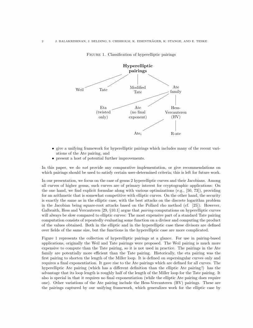
Figure 1. Classification of hyperelliptic pairings

Hyperellipticpairings

kkkkkkkkkkkkkkkkkkkk

rrrrrrrrrrrr

MMMMMMMMMMMM

Weil Tate ModifiedTate

Atefamily

iiiiiiiiiiiiiiiiiiiiiiiiiiiiii

rrrrrrrrrrrr

Eta(twistedonly)

Ate(no final

exponent)

Hess-Vercauteren

(HV)

pppppppppppp

Atei R-ate

• give a unifying framework for hyperelliptic pairings which includes many of the recent vari-ations of the Ate pairing, and

• present a host of potential further improvements.

In this paper, we do not provide any comparative implementation, or give recommendations onwhich pairings should be used to satisfy certain user-determined criteria; this is left for future work.

In our presentation, we focus on the case of genus 2 hyperelliptic curves and their Jacobians. Amongall curves of higher genus, such curves are of primary interest for cryptographic applications: Onthe one hand, we find explicit formulae along with various optimizations (e.g., [50, 73]), providingfor an arithmetic that is somewhat competitive with elliptic curves. On the other hand, the securityis exactly the same as in the elliptic case, with the best attacks on the discrete logarithm problemin the Jacobian being square-root attacks based on the Pollard rho method (cf. [25]). However,Galbraith, Hess and Vercauteren [29, §10.1] argue that pairing computations on hyperelliptic curveswill always be slow compared to elliptic curves: The most expensive part of a standard Tate pairingcomputation consists of repeatedly evaluating some function on a divisor and computing the productof the values obtained. Both in the elliptic and in the hyperelliptic case these divisors are definedover fields of the same size, but the functions in the hyperelliptic case are more complicated.

Figure 1 represents the collection of hyperelliptic pairings at a glance. For use in pairing-basedapplications, originally the Weil and Tate pairings were proposed. The Weil pairing is much moreexpensive to compute than the Tate pairing, so it is not used in practice. The pairings in the Atefamily are potentially more efficient than the Tate pairing. Historically, the eta pairing was thefirst pairing to shorten the length of the Miller loop. It is defined on supersingular curves only andrequires a final exponentiation. It gave rise to the Ate pairings which are defined for all curves. Thehyperelliptic Ate pairing (which has a different definition than the elliptic Ate pairing !) has theadvantage that its loop length is roughly half of the length of the Miller loop for the Tate pairing. Italso is special in that it requires no final exponentiation (while the elliptic Ate pairing does requireone). Other variations of the Ate pairing include the Hess-Vercauteren (HV) pairings. These arethe pairings captured by our unifying framework, which generalizes work for the elliptic case by

PAIRINGS ON HYPERELLIPTIC CURVES 3

Hess [40] and Vercauteren [71]. HV pairings also have potentially shorter Miller loops than the Atepairing, depending on the embedding degree of the Jacobian. All of the HV pairings involve a finalexponentiation. Two examples of HV pairings are the R-ate and the Atei pairings. Table 5.6 inSection 5 gives more details about the differences and merits of each pairing.

Our paper is organized as follows. In Section 2 we review some of the background on Jacobians ofhyperelliptic curves. Section 3 discusses hyperelliptic curves of low embedding degree and what isknown about constructing them. Section 4 gives an overview of the different pairings on hyperellipticcurves following the classification in Figure 1. We also introduce the HV pairing framework, givea direct proof of the non-degeneracy and bilinearity of the pairings captured by this frameworkand discuss how the Ate and R-ate pairings fit in. Section 5 describes the adaptation of Miller’salgorithm to the hyperelliptic setting, presents common optimizations and compares all pairingsaccording to their key characteristics of loop length and final exponentiation. Section 6 presentsnumerous problems for future work.

2. Jacobians of Hyperelliptic Curves

In this section, we fix some notation and terminology that will be used throughout the paper.

2.1. Hyperelliptic curves. A hyperelliptic curve C over a field K is a non-singular projectivecurve of the form

C : y2 +H(x)y = F (x) ∈ K[x, y].

Let g be the genus of the curve. Throughout this paper, we restrict to the case where F is monic,degF (x) = 2g+1, and degH(x) ≤ g, so that C has one point at infinity, denoted P∞. When g = 1,C is an elliptic curve. For significant parts of our discussion, we will consider the case where g = 2.

Although the points of a genus g ≥ 2 hyperelliptic curve do not form a group, there is an involutionof the curve taking P = (x, y) to the point (x,−y − H(x)), which we will denote −P . Then, inaccordance with the notation, −(−P ) = P .

2.2. Divisors and abelian varieties. Let K be a field over which C is defined, and let K itsalgebraic closure. A divisor D on the curve C is a formal sum over all symbols (P ), where P is aK-point of the curve:

D =∑

P∈C(K)

nP (P ),

where all but finitely many of the coefficients nP ∈ Z are zero. The collection of divisors forms anabelian group Div(C). The degree of a divisor is the sum∑

P∈C(K)

nP ∈ Z,

and the support of a divisor is the set of points of the divisor with non-zero coefficients nP . For anyrational function f on C, there is an associated divisor

div(f) =∑

P∈C(K)

ordP (f)(P )

which encodes the number and location of its zeroes and poles. Any divisor which is the divisor ofa function in this way is called a principal divisor.


An element σ in the Galois group of K over K, Gal(K/K), acts on a divisor as follows:( ∑P∈C(K)

nP (P ))σ

=∑

P∈C(K)

nP (Pσ).

In particular, let L be any intermediate field K ⊂ L ⊂ K. Consider a function f defined over L;then div(f) is fixed by elements of Gal(K/L). In fact, div(f)σ = div(fσ).

We give names to various sets of collections: Div(C) of divisors, Div0(C) of degree zero divisors,Ppl(C) of principal divisors, DivK(C) of divisors invariant under the action of Gal(K/K), Div0

K(C)of degree zero divisors invariant under the action of Gal(K/K), and PplK(C) of principal divisorsinvariant under the action of Gal(K/K).

These are all abelian groups, which have the following subgroup relations:

Div(C) ⊃ Div0(C) ⊃ Ppl(C)

∪ ∪ ∪

DivK(C) ⊃ Div0K(C) ⊃ PplK(C).

We make note of certain quotient groups:

Pic(C) := Div(C)/Ppl(C), Pic0(C) := Div0(C)/Ppl(C),

PicK(C) := DivK(C)/PplK(C), Pic0K(C) := Div0

K(C)/PplK(C).

Elements of these quotient groups are equivalence classes of divisors. Divisors D1 and D2 of thesame class are said to be linearly equivalent, and we write D1 ∼ D2.

Recall that an elliptic curve is an example of an abelian variety. In general, an abelian variety Aover K is a projective algebraic variety over K along with a group law ϕ : A×A→ A and an inversemap Inv : A → A sending x 7→ x−1 such that ϕ and Inv are morphisms of varieties, both definedover K.

For an abelian variety A, a field K and an integer r, we let A(K)[r] denote the set of r-torsionpoints of A defined over K, that is, the set of points in A(K) of order dividing r. Now supposeA is an abelian variety over Fq, with q = pm. We say that A is simple if it is not isogenous overFq to a product of lower dimensional abelian varieties. We call A absolutely simple if it is simpleover Fq. We say A is supersingular if A is isogenous over Fq to a power of a supersingular ellipticcurve. (An elliptic curve E is supersingular if E(Fq) has no points of order p.) An abelian varietyA of dimension g over Fq is ordinary if #A(Fq)[p] = pg. Note that for dimension g ≥ 2, there existabelian varieties that are neither ordinary nor supersingular.

There is a natural isomorphism between the degree zero part of the Picard group Pic0(C) of ahyperelliptic curve C and its Jacobian JacC , which is an abelian variety into which the curve embeds(cf. [26]). For the remainder of this paper, we will identify the Picard group Pic0(C) with JacC .


2.3. Arithmetic in the Jacobian. We will work in the Jacobian JacC of a hyperelliptic curve Cof genus g, whose elements are equivalence classes of degree-zero divisors. To do so, we choose areduced representative in each such divisor class. A reduced divisor is one of the form

(P1) + (P2) + · · ·+ (Pr)− r(P∞)

where r ≤ g, P∞ is the point at infinity on C, Pi 6= −Pj for distinct i and j, and no Pi satisfyingPi = −Pi appears more than once. Such a divisor is called semi-reduced if the condition r ≤ g isomitted. Each equivalence class contains exactly one reduced divisor. For a divisor D we will denoteby ρ(D) the reduced representative of its equivalence class. The action of Galois commutes with ρ,i.e. ρ(Dσ) = ρ(D)σ, since the property of being reduced is preserved by the action of Galois.

To encode the reduced divisor in a convenient way, we write (u(x), v(x)) where u(x) is a monicpolynomial whose roots are the x-coordinates x1, . . . , xr of the r points

P1 = (x1, y1), . . . , Pr = (xr, yr),

and where v(xi) = yi for i = 1, . . . , r. This so-called Mumford representation [59] is uniquelydetermined by and uniquely determines the divisor. To find this representation, it suffices to findu(x) and v(x) satisfying the following conditions:

(1) u(x) is monic,(2) deg(v(x)) < deg(u(x)) ≤ g, and(3) u(x) | F (x)− v(x)H(x)− v(x)2,

where F (x) andH(x) are the polynomials defining the curve C (defined in Section 2.1). When we addtwo reduced divisors D1 and D2 the result D1 +D2 is not necessarily reduced. Beginning with tworeduced divisors in Mumford representation, the algorithm to obtain the Mumford representation ofthe reduction of their sum can be explained in terms of the polynomials involved in the Mumfordrepresentation, without recourse to the divisor representation. This algorithm is originally due toCantor [6], and in the form presented here to Koblitz [47]. The algorithm has two stages: in thefirst, we find a semi-reduced divisor D ∼ D1 +D2, and in the second stage, we reduce D. Supposethat Di has Mumford representation (ui, vi) for i = 1, 2.

Stage 1:

(1) Find d(x) = gcd(u1(x), u2(x), v1(x) + v2(x) + H(x)). Finding this via the extendedEuclidean algorithm gives s1(x), s2(x) and s3(x) such that

d = s1u1 + s2u2 + s3(v1 + v2 +H).

(2) Calculate the quantities

u = u1u2/d2, and v = s1u1v2 + s2u2v1 + s3(v1v2 + F )/d (mod u(x)) .

(It is easily verified that the fraction on the right is defined since d(x) is a divisor of thenumerator.)

At this point, the result (u, v) is a semi-reduced divisor linearly equivalent to D1 + D2. Thisstage corresponds to simply adding D1 and D2 and canceling any points with their negatives ifapplicable. In fact, we obtain

D′ = D1 +D2 − div(d).

Stage 2:


In this stage, if deg(u) > g we can replace (u, v) with a divisor (u′, v′) satisfying deg(u′) < deg(u).This replacement is as follows. Set

u′ = (F − vH − v2)/u, and v′ = −H − v (mod u′) .

This stage corresponds to simplifying the divisor using the geometric group law nicely describedfor genus 2 by Lauter [51]. At each application of this loop to a divisor D3, we obtain a divisorD′′ satisfying1

D′′ = D3 − div((F − vH − v2)/u′).Applying this loop finitely many times, beginning with the result D′ of stage one, we eventuallyobtain a reduced divisor D linearly equivalent to D1 +D2.

This algorithm has been optimized to avoid the use of the extended Euclidean algorithm and in thisform it is much more efficient [29]. An enhanced version of Cantor’s Algorithm is given as Algorithm2 in this paper; see Section 5.1. If steps 5 and 8 through 13 are removed from Algorithm 2 one hasthe Cantor’s Algorithm discussed here.

3. Hyperelliptic Curves of Low Embedding Degree

In this section we discuss hyperelliptic curves suitable for pairing-based cryptographic systems. TheJacobian varieties of such curves must have computable pairings, and computationally infeasiblediscrete logarithm problems. Specifically, we require low embedding degrees and large prime-ordersubgroups.

3.1. Embedding degree and ρ-value. Let r be a prime. Let C be a hyperelliptic curve over Fq ofgenus g with Jacobian variety JacC(Fq) such that r | # JacC(Fq) and gcd(r, q) = 1. The embeddingdegree of JacC with respect to r is the smallest integer k such that r | (qk − 1). Equivalently, theembedding degree of JacC with respect to r is the smallest integer k such that F∗qk contains thegroup of rth roots of unity µr. If JacC has embedding degree k with respect to r, then a pairingon C, such as the Weil pairing er : JacC(Fq)[r] × JacC(Fq)[r] → µr, “embeds” JacC(Fq)[r] (andany discrete logarithm problem in JacC(Fq)[r]) into F∗qk , and Fqk is the smallest-degree extension ofFq with this property; whence the name “embedding degree”. Hitt [42] shows that if q = pm withm > 1, then JacC(Fq)[r] may be embedded into a smaller field which is not an extension of Fq butonly an extension of Fp. The smallest such field is the so-called minimal embedding field, which isFpordr p .

We occasionally speak of the embedding degree of the hyperelliptic curve C, in which case we meanthe embedding degree of its Jacobian.

Another important parameter is the ρ-value, which for a Jacobian variety of dimension g we define asρ = g log q/ log r. Since #JacC(Fq) = qg +O(qg−1/2), the ρ-value measures the ratio of the bit-sizesof # JacC(Fq) and the subgroup order r. Jacobian varieties with a prime number of points have thesmallest ρ-values: ρ ≈ 1. We call a hyperelliptic curve, and its Jacobian variety, pairing-friendly ifthe Jacobian variety has small embedding degree and a large prime-order subgroup. In practice, wewant k ≤ 60 and r > 2160.

Since the embedding degree k is the order of q in the multiplicative group (Z/rZ)∗, and typicallyelements in (Z/rZ)∗ have large order, we expect that for a random Jacobian over Fq with order-rsubgroup, the embedding degree is approximately of the same size as r. (This reasoning has been

1In general, u′ is a product of lines Li whose divisors are (Pi)+(−Pi)−2(P∞) for i = 1, . . . , r and div(F−vH−v2)is the sum of the intersection points of C and a unique curve intersecting C at 3g points including P1, . . . , Pr.


made more precise for elliptic curves, by Balasubramanian and Koblitz [1] and Luca, Mireles andShparlinski [57].) With r > 2160, this means that evaluating a pairing for a random hyperellipticcurve becomes a computationally infeasible task. Just as in the case of elliptic curves, pairing-friendlyhyperelliptic curves are rare and require special constructions.

3.2. Embedding degrees required for various security levels. For cryptographic applications,the discrete logarithm problems in JacC(Fq) and in the multiplicative group F∗qk must both becomputationally infeasible. For Jacobian varieties of hyperelliptic curves of genus 2 the best knowndiscrete logarithm (DL) algorithm is the parallelized Pollard rho algorithm [70, 65], which hasrunning time O(

√r) where r is the size of the largest prime-order subgroup of JacC(Fq). For Jacobian

varieties of dimensions 3 and 4 there exist index calculus algorithms of complexities O(q4/3+ε) =O(| JacC |4/9+ε) and O(q3/2+ε) = O(| JacC |3/8+ε), respectively [35]. How this compares to theparallelized Pollard rho algorithm depends on the relative size of the subgroup order r – moreprecisely, only if ρ < 9/8 (genus 3 case) or ρ < 4/3 (genus 4 case) will the index calculus approachbe superior to Pollard rho.

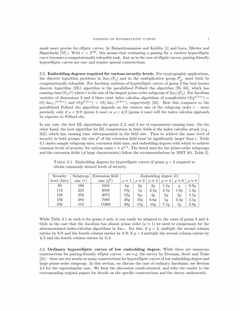
In any case, the best DL algorithms for genus 2, 3, and 4 are of exponential running time. On theother hand, the best algorithm for DL computation in finite fields is the index calculus attack (e.g.,[62]) which has running time subexponential in the field size. Thus to achieve the same level ofsecurity in both groups, the size qk of the extension field must be significantly larger than r. Table3.1 shows sample subgroup sizes, extension field sizes, and embedding degrees with which to achievecommon levels of security, for various cases r ≈ qg/ρ. The listed sizes for the prime-order subgroupsand the extension fields (of large characteristic) follow the recommendations by NIST [61, Table 2].

Table 3.1. Embedding degrees for hyperelliptic curves of genus g = 2 required toobtain commonly desired levels of security.

Security Subgroup Extension field Embedding degree (k)level (bits) size (r) size (qk) ρ ≈ 1 ρ ≈ 2 ρ ≈ 3 ρ ≈ 4 ρ ≈ 6 ρ ≈ 8

80 160 1024 6g 3g 2g 1.5g g 0.8g112 224 2048 10g 5g 3.3g 2.5g 1.6g 1.3g128 256 3072 12g 6g 4g 3g 2g 1.5g192 384 7680 20g 10g 6.6g 5g 3.3g 2.5g256 512 15360 30g 15g 10g 7.5g 5g 3.8g

While Table 3.1 as such is for genus 2 only, it can easily be adapted to the cases of genus 3 and 4:Only in the case that the Jacobian has almost prime order (ρ ≈ 1) we need to compensate for theaforementioned index-calculus algorithms in JacC . For this, if g = 3, multiply the second columnentries by 9/8 and the fourth column entries by 8/9; if g = 4 multiply the second column entries by4/3 and the fourth column entries by 3/4.

3.3. Ordinary hyperelliptic curves of low embedding degree. While there are numerousconstructions for pairing-friendly elliptic curves – see e.g. the survey by Freeman, Scott and Teske[21] – there are not nearly as many constructions for hyperelliptic curves of low embedding degree andlarge prime-order subgroup. In this section, we discuss the case of ordinary Jacobians; see Section3.4 for the supersingular case. We keep the discussion result-oriented, and refer the reader to thecorresponding original papers for details on the specific constructions and the theory underneath.


Galbraith, McKee and Valenca [32] argue that heuristically, for any fixed embedding degree k withϕ(k) ≥ 4 (ϕ(k) = the Euler phi-function) and for any bound M on the field size q, there existabout as many genus 2 curves over Fq of embedding degree k (any ρ-value) as there exist ellipticcurves over Fq of embedding degree k, namely Θ(M1/2/ logM). For embedding degrees k = 5, 10,they identify several quadratic polynomials q(x) parameterizing field sizes such that genus 2 curvesover Fq(x) exist with embedding degree k (any ρ-value). (They also show that for k = 8, 12, suchquadratic polynomials q(x) do not exist.)

Freeman [18] was the first to actually construct ordinary genus 2 curves of low embedding degree.His construction is based on the Cocks-Pinch method [11][21, Theorem 4.1], which produces pairing-friendly elliptic curves over prime fields of any prescribed embedding degree and with ρ ≈ 2. In thegenus-2 case, Freeman obtains curves over prime fields Fq of any prescribed embedding degree k andρ-value 8, that is, r ≈ q1/4 (where r denotes the prime subgroup order of the Jacobian).

Freeman [18, Proposition 2.3] further shows that the resulting Jacobian varieties have the propertythat JacC(Fqk) always contains two linearly independent r-torsion points. For an elliptic curveE/Fq, the corresponding result implies that the entire r-torsion group is contained in E(Fqk), butthis is not necessarily the case for higher dimensional abelian varieties. This phenomenon givesrise to the notion of the full embedding degree, which is the smallest integer k such that all r-torsion points of JacC are defined over Fqk . Freeman [18, Algorithm 5.1] gives a construction ofgenus 2 curves of prescribed full embedding degree k (necessarily even), which may be useful incryptographic applications that require more than two linearly independent r-torsion points (seeSection 6.8). Again, this construction yields curves with ρ-value 8.

Note that an essential part of either construction [18] is the use of the complex multiplication (CM)method to compute the actual curve. In genus 2, this includes computation of the Igusa classpolynomials (e.g., [72]) of the CM field K = End(JacC)⊗Q, which is currently feasible for CM fieldsK with class numbers less than 100 [49]. (Here, End(JacC) denotes the set of all endomorphisms ofJacC defined over Fq.)

Freeman, Stevenhagen and Streng [22, Algorithm 2.12] present a generalization of the Cocks-Pinch method, which, when coupled with complex multiplication methods, produces pairing-friendlyabelian varieties over prime fields, of dimension g with ρ-values ≈ 2g2. This algorithm works forany prescribed embedding degree k, and applies to arbitrary genus g ≥ 2. (However note thatcomplex multiplication methods are available for special CM fields only if g = 3, and are completelyundeveloped for g ≥ 4.) In addition to explicit genus 2 examples with ρ ≈ 8, a cryptographicallyinteresting example is given for genus 3 (k = 17 and ρ ≈ 17.95).

In the case of pairing-friendly elliptic curves, the method by Brezing and Weng [5] is a generalizationof the Cocks-Pinch method [11] and produces elliptic curves over prime fields with 1 < ρ < 2 formany embedding degrees. Freeman [19, Algorithm 3.8] combines the Brezing-Weng approach withthe method from Freeman, Stevenhagen and Streng [22] to construct so-called families of abelianvarieties over prime fields with ρ-values strictly less than 2g2. An explicit construction for genus2, embedding degree k = 5 and ρ = 4 is given – note that an instantiation with a 224-bit primesubgroup order r would exactly meet the 112-bit security level requirements (cf. Table 3.1). Otherexamples (for genus 2) include: k = 6, ρ = 7.5; k = 8, ρ = 7.5, and k = 10, ρ = 6 (able to exactlymeet the 256-bit security level requirements) [19, 17]. In the case of genus 3, a construction yieldingk = 7 and ρ = 12 is obtained.

All constructions mentioned so far in this section produce absolutely simple Jacobians. Whenconsidering simple abelian varieties A that are isogenous over some extension field Fqd (q a prime)


to a product of two elliptic curves, smaller ρ-values have been obtained:Kawazoe and Takahashi [45] specialize to hyperelliptic curves with curve equation y2 = x5 + axover a prime field Fq. For the cardinalities of the Jacobians of such curves, closed formulae exist.These formulae are exploited in adaptations of the Cocks-Pinch method (producing Jacobians withρ-values around 4), and Brezing-Weng-type methods (for embedding degree divisible by 8, producingJacobian varieties with 3 < ρ < 4). The Jacobians split over Fqd , d ∈ {2, 4}.Satoh [67] considers hyperelliptic curves C of the form y2 = x5 + ax3 + bx over Fq, such that JacC

splits over Fq2 . This construction works for many embedding degrees and produces ρ-values < 4.More generally, Freeman and Satoh [20] show that if E is defined over Fq, and A is an abelianvariety isogenous over Fqd to E × E, then A is isogenous over Fq to a primitive subvariety of theWeil restriction of E from Fqd to Fq. Thus, pairing-friendly abelian varieties of this type can bebuilt from elliptic curves E/Fq that are not pairing-friendly over Fq, but are pairing-friendly whenbase-extended to Fqd . The elliptic curves can be constructed via Cocks-Pinch or Brezing-Weng typemethods. The generic ρ-value for Jacobians of genus 2 produced in this manner is 4. With theBrezing-Weng method, ρ-values between 2 and 4 can be obtained. This approach not only containsthe constructions by Kawazoe and Takahashi [45] and Satoh [67] but also produces the lowest everrecorded ρ-values for ordinary genus 2 curves. Explicit examples of cryptographically interestinggenus 2 curves are given, such as a k = 9, ρ ≈ 8/3 curve and a k = 27, ρ ≈ 20/9 curve.

In conclusion, to date, the best we can achieve for pairing-friendly ordinary genus 2 curves witharbitrary prescribed embedding degree k is a ρ-value of 4; and ρ ≈ 8 if one insists on absolutelysimple Jacobians. (Although to date, there is no apparent reason why Jacobians that split oversmall-degree extensions should be more vulnerable to DL attacks than the absolutely simple ones.)We have no constructions of ordinary hyperelliptic curves of genus g ≥ 2 with ρ-values less than2. In particular, we have no constructions of higher-dimensional pairing-friendly ordinary Jacobianvarieties with a prime number of points. This is in sharp contrast to the elliptic case, where ρ ≈ 2can be achieved for any prescribed embedding degree, 1 < ρ < 2 for selected embedding degrees,and constructions for prime-order elliptic curves exist for embedding degrees k = 3, 4, 6, 10, and 12(cf. [21]).

3.4. Supersingular curves. Supersingular hyperelliptic curves over Fq are always pairing-friendly.In fact, Galbraith [28] shows that there exists a constant k(g) such that the embedding degree of anysupersingular abelian variety of dimension g over any finite field Fq is bounded by k(g). Rubin andSilverberg [66] prove that for simple supersingular abelian varieties, for g ≤ 6 we have k(g) ≤ 7.5g.

Specifically, for dimension g = 2, the embedding degree is bounded by 12, where k = 12 can onlyhappen if Fq is a binary field F2m with m odd. If q is a square, or if q = pm with m odd andp 6= 2, 3, then the largest embedding degree is k = 6. If Fq = F3m with m odd, the embeddingdegree is always bounded by 4. (In the case of dimension g = 3, the embedding degree is boundedby 18, and the bound for the dimension 4 case is 30. In both cases, this bound is achieved only incharacteristic three. Over prime fields Fp with p ≥ 11, there are no simple supersingular abelianvarieties of dimension g = 3, while the largest embedding degree for dimension g = 4 is k = 12.)

As Rubin and Silverberg show [66, Corollaries 13,14], not all embedding degrees below these boundsare possible. For example, in the dimension 2 case and if q = pm with m odd, then for p = 2 wehave k ∈ {1, 3, 6, 12}; if p = 3, we have k ∈ {1, 3, 4}; if p = 5 we have k ∈ {1, 3, 4, 5, 6} and if p ≥ 7we have k ∈ {1, 3, 4, 6}.

Cryptographically interesting supersingular hyperelliptic curves can be explicitly constructed. Forexample, Galbraith et al. [33] give curve equations for various field characteristics that yield simple


supersingular Jacobians of dimension g = 2 and of embedding degrees k ∈ {4, 5, 6, 12}. By carefullychoosing the underlying fields, ρ-values close to 1 can be readily obtained.

3.5. Supersingular versus ordinary hyperelliptic curves. While the embedding degrees ofsupersingular abelian varieties are limited to a few, small values, their advantage is that they canachieve ρ-values significantly smaller than their ordinary counterparts. For example, let us considerthe 112-bit security level (cf. Table 3.1). One could use the construction by Freeman and Satoh [20]of an ordinary absolutely simple hyperelliptic Jacobian of dimension 2, with embedding degree k = 6and ρ-value 2.976, with a 230-bit prime-order subgroup, working over a finite field Fq with 342-bitq. Alternatively, one could use the embedding-degree 12 supersingular curve y2 + y = x5 + x3 + b(b ∈ {0, 1}) over F2m with m ≥ 250 chosen such that its Jacobian contains a subgroup of primeorder r > 2224. (Note that Coppersmith’ algorithm [12] for DL computation in finite fields ofsmall characteristic requires to embed the Jacobian into a 3000-bit binary field F212m , to obtainroughly the same level of security provided by a 2048-bit field Fq12 with q large, cf. [55].) If m ischosen smaller than 342, this would result in bandwidth advantages for the supersingular Jacobian,given that in cryptographic applications the values that are transmitted are elements in JacC(Fq).However, already at the 128-bit security level the advantage of supersingular curves disappears, inthe light of the recent work by Freeman and Satoh [20]: this security level can be achieved with256-bit prime-order subgroups either of an ordinary Jacobian over a 341-bit Fq, with k = 9 andρ = 8/3, or of a supersingular Jacobian over F2m with m ≥ 375, of embedding degree 12 (again, mis chosen in response to Coppersmith’ DL algorithm [12]: a 4500-bit binary field roughly providesthe same security as a 3072-bit field of large characteristic). At high security levels ordinary curvesare definitely preferable. For example, at the 256-bit level, a genus 2 curve with embedding degreek = 27 and (optimal to date) ρ-value of 20/9 (cf. [20]) requires a 568-bit field, while a binarysupersingular curve of embedding degree 12 requires a 1875-bit field.

4. Pairings for Hyperelliptic Curves

In this section, we give an overview of the different pairings on hyperelliptic curves, as well asintroduce the more general framework of HV pairings which unify the recent variations on the Atepairing. In particular, we present a direct proof of bilinearity and non-degeneracy for these pairingsand describe how the Atei and R-ate pairings fit into the framework.

We begin by introducing the historically most important pairings for hyperelliptic curves, the Tate-Lichtenbaum and Weil pairings. In what follows, let r be a positive integer and assume that C isdefined over a finite field Fq. Suppose that K = Fqk is an extension of Fq such that r | (qk − 1).Throughout the section, we will use D to mean both a divisor and the divisor class represented byD.

For a positive integer s, a Miller function fs,D is a function with divisor

(fs,D) = sD − ρ(sD),

uniquely defined up to scalar multiplication by elements of K∗. The Miller loop length of such afunction is log2 s and measures how quickly the function can be evaluated via Miller’s algorithm(see Algorithm 1). The benefit of recent variations on the Tate-Lichtenbaum pairing is a reductionin Miller loop length, which is sometimes accomplished by combining several Miller functions (seeSection 5).


4.1. Tate-Lichtenbaum pairing. For D1 ∈ JacC(K)[r], the divisor rD1 is linearly equivalent tozero, hence there is some function whose divisor is rD1, namely the Miller function fr,D1 definedabove. Let D2 be a divisor class, with representative D2 =

∑P nP (P ) disjoint from D1. We define

a pairing called the Tate-Lichtenbaum pairing as follows

τ : JacC(K)[r]× JacC(K)/rJacC(K) → K∗/(K∗)r

(D1, D2) 7→ fr,D1(D2) =∏P

fr,D1(P )nP .

This pairing is bilinear, non-degenerate and the result is independent of the choice of representativesof the divisor classes.

4.2. The Weil pairing. For D1, D2 ∈ JacC(K)[r], the Weil pairing is given by

er : JacC(K)[r]× JacC(K)[r] → µr

(D1, D2) 7→ τ(D1, D2)τ(D2, D1)−1

which can be computed via two Tate-Lichtenbaum pairings. It is bilinear, alternating, and non-degenerate.

4.3. The modified Tate-Lichtenbaum pairing. If JacC(K) contains no elements of order r2,then there is an isomorphism

JacC(K)[r] ∼= JacC(K)/rJacC(K).

Under this identification, we define the modified (or reduced) Tate-Lichtenbaum pairing to be

t : JacC(K)[r]× JacC(K)[r] → µr

(D1, D2) 7→ τ(D1, D2)(qk−1)/r.

Since elements ofK∗ have order dividing qk−1 and r | (qk−1), the rth powers which are the quotientsof distinct representatives of the coset of τ(D1, D2) are removed by this final exponentiation, leavinga unique result lying in µr ⊂ K.

Other powers of the Tate-Lichtenbaum pairing can also give non-degenerate bilinear pairings intoµr which may yield shorter Miller loops (for example, with the use of efficiently computable auto-morphisms of C [16]; see Section 6.2).

4.4. Hyperelliptic Ate pairing. More generally, a bilinear pairing is a map

e : G1 ×G2 → G3

where Gi are abelian groups, in additive notation, and G3 is a cyclic group, written multiplicatively,and for all p1, p2 ∈ G1, q1, q2 ∈ G2, we have

e(p1 + p2, q1) = e(p1, q1)e(p2, q1),

e(p1, q1 + q2) = e(p1, q1)e(p1, q2).

Let r be a prime dividing #JacC(Fq) and let k be the embedding degree of JacC(Fq) with respectto r. We are interested in pairings where G1 and G2 are subgroups of JacC(K), where K = Fqk . Inparticular, a number of more convenient and faster pairings are known when

(4.1)G1 = JacC(K)[r] ∩ ker(π − [1]),G2 = JacC(K)[r] ∩ ker(π − [q]),


where π is the qth power Frobenius automorphism. Since r divides #JacC(Fq), the group G1, beingthe eigenspace of 1, is at least 1-dimensional over Z/rZ. Since the eigenvalues of the Frobeniuscome in pairs (λ, q/λ) [27, §5.2.3], q is also an eigenvalue of π on JacC [r], and thus there exists adivisor D such that π(D) = qD. This implies that πkD = qkD = D, since r|(qk − 1) and rD = 0.Consequently, D ∈ JacC(Fqk), and the group G2 is also at least 1-dimensional over Z/rZ. If k > 1,then G1 6= G2 and G1 × G2 ⊂ JacC(Fqk)[r] is at least 2-dimensional over Z/rZ. (Recall that forgenus g, the group JacC(K)[r] is 2g-dimensional over Z/rZ.)

In the remainder of this section, G1 and G2 always denote the groups defined in (4.1).

The most basic pairing defined for divisors in G1, G2 is the hyperelliptic Ate pairing [36]:

a : G2 ×G1 → µr

(D2, D1) 7→ fq,ρ(D2)(D1),

where ρ(D2) is the reduced divisor class representative. Since the Frobenius π acts as [q] on D2, wehave fq,ρ(D2)(D1) ∈ µr and no final exponentiation is required [36, Lemma 2]. This is different fromthe elliptic Ate pairing [41], where a final exponentiation is always required. Another importantdifference of the hyperelliptic Ate pairing is that to obtain a well-defined value, one must use thereduced divisor ρ(D2), not simply any representative of the class D2. The Miller loop length forthe hyperelliptic Ate pairing is log2 q, in contrast to the elliptic case where the Miller loop length islog2(t− 1) with t the trace of Frobenius.

4.5. The Hess-Vercauteren (HV) framework for pairings on Frobenius eigenspaces. Since2007, several variations of the Ate pairing have been proposed for elliptic and hyperelliptic curves,exploiting the fact that products and ratios of bilinear, non-degenerate pairings on G2×G1 are alsobilinear pairings, but not necessarily non-degenerate [75]. The key is to find combinations of pairingswhich are both non-degenerate and computable using shorter Miller loops. Following the work ofHess [40] and Vercauteren [71] in the elliptic curve case, we unify these various pairings on G2 ×G1

in a more general framework, which we call HV pairings. The main benefit of this framework is thatthe criteria for non-degeneracy are more straightforward to verify, giving a direct way to create newpairings. Further investigation of this framework and possible extensions seems likely to be fruitful(see Section 6.1 and (1) in Section 6.9).

Let D be any divisor in JacC(K)[r], and s an integer. Recall that any divisor D is equivalent toa unique reduced divisor which we denote ρ(D). Let h(x) ∈ Z[x] be a polynomial of the formh(x) =

∑ni=0 hix

i satisfying h(s) ≡ 0 (mod r). Define a generalized Miller function fs,h,D to be anyfunction with divisor

(4.2)n∑

i=0

hiρ(siD).

To see that this divisor is principal, consider the principal divisorn∑

i=0

hi(siD − ρ(siD)),

which differs by (∑n

i=0 hisi)D from (4.2). Since h(s) ≡ 0 (mod r), this is an integer multiple of

rD, which is linearly equivalent to zero by assumption, and thus the divisor (4.2) is principal. Aswith the standard Miller function, the function fs,h,D is only defined up to scalar multiples. Also,we note that the Miller function fr,D for the Tate-Lichtenbaum pairing is equal to fs,h,D for theconstant function h(x) = r and arbitrary integer s.


Theorem 4.1. Let s ≡ qj (mod r) for some j ∈ Z. Let h(x) ∈ Z[x] with h(s) ≡ 0 (mod r). Then

as,h : G2 ×G1 → µr

(D2, D1) 7→ fs,h,D2(D1)(qk−1)/r

is a bilinear pairing satisfying

as,h(D2, D1) = t(D2, D1)h(s)/r and as,h(D2, D1) = a(D2, D1)kqk−1h(s)/r

where t is the modified Tate-Lichtenbaum pairing and a is the hyperelliptic Ate pairing. The pairingas,h is non-degenerate if and only if h(s) 6≡ 0

(mod r2

).

Remark 4.2. We note that since k is the embedding degree of JacC(Fq) with respect to r, inTheorem 4.1 s will be a kth root of unity modulo r since q is a primitive kth root. In Hess’sframework, there is the additional condition that s be a primitive kth root of unity modulo r2. Thisrequirement is necessary to show the existence of pairings such that the function fs,h,D is of “lowestdegree” (see [40, §3]), but is not required for the result above.

Proof. First we show that the pairing is well-defined on divisor classes. Suppose that D′2 ∼ D2.

Then

div(fs,h,D′2/fs,h,D2) =

n∑i=1

hi(ρ(siD′2)− ρ(siD2)) = ∅.

This demonstrates well-definition in the factor G2. For the factor G1, it suffices to show that thepairing is trivial under the hypothesis that D1 is a principal divisor. Suppose D1 = div(g). For anyD2 ∈ G2, by the hypothesis that s ≡ qj mod r and ρ(rD2) = ∅, it is the case that

ρ(siD2) = ρ(qijD2) = ρ(πijD2) = πijρ(D2) = qijρ(D2) = siρ(D2) + rD′

for some divisor D′ defined over Fq. Therefore,n∑

i=1

hiρ(siD2) =n∑

i=1

hisiρ(D2) + rD′′

for some D′′ defined over Fq. Then by the hypothesis, this expression is an r-th multiple of anotherdivisor D′′′ defined over Fq. By Weil reciprocity,

fs,h,D2(D1)(qk−1)/r = g(rD′′′)(q

k−1)/r = g(D′′′)qk−1 = 1,

as required.

We show bilinearity and non-degeneracy directly, in contrast to Hess’s more general approach in theelliptic curve case [40, Theorem 1].

Let s = qj + `r, for j, ` ∈ Z. Linearity in the second coordinate follows from the definition ofevaluation of a function on a divisor. To show linearity in the first coordinate, let D2, D3 ∈ G2 andD1 ∈ G1 be non-trivial reduced divisors. Then

(fs,h,D2+D3) =n∑

i=0

hiρ(siD2 + siD3) =n∑

i=0

hiρ(siD2) +n∑

i=0

hiρ(siD3) +n∑

i=0

hi(gi)

where(gi) = ρ(siD2 + siD3)− ρ(siD2)− ρ(siD3).

Since rD2 ∼ 0, rD3 ∼ 0 and s = qj + `r, the function gi has divisor

(gi) = ρ(qijD2 + qijD3)− ρ(qijD2)− ρ(qijD3).


Since D2, D3 ∈ G2, the q-eigenspace of the Frobenius π, and since ρ commutes with π, we have

(gi) = ρ(D2 +D3)πij

− ρ(D2)πij

− ρ(D3)πij

.

Then (gi) = (m)πij

where m is the function with divisor

(m) = ρ(D2 +D3)− ρ(D2)− ρ(D3).

As fs,h,D2+D3 is evaluated at the divisor D1 ∈ G1, which is fixed by π, the value gi(D1) equalsm(D1)πij

= m(D1)qij

. Thus,n∏

i=0

gi(D1)hi =n∏

i=0

m(D1)hiqij

= m(D1)Pn

i=0 hiqij

= m(D1)h(qj).

Using the fact that s = qj + `r and h(s) ≡ 0 (mod r), we see that this value is eliminated by thefinal exponentiation of (qk − 1)/r. Since

fs,h,D2+D3(D1) = fs,h,D2(D1)fs,h,D3(D1)n∏

i=0

gi(D1)hi ,

the pairing as,h is linear with respect to the first coordinate.

We now show thatas,h(D2, D1) = t(D2, D1)h(s)/r

using a similar argument. On the right, we have

t(D2, D1)h(s)/r =(fr,D2(D1)(q

k−1)/r)h(s)/r

.

Since D2 ∈ G2, we have ρ(rD2) = 0, thus

(f h(s)/rr,D2

) = (h(s)/r)(rD2 − ρ(rD2)) = h(s)D2 =n∑

i=0

hisiD2.

On the left, we haveas,h(D2, D1) = fs,h,D2(D1)(q

k−1)/r.

where by definition

(fs,h,D2) =n∑

i=0

hiρ(siD2).

We can rewrite this as

(fs,h,D2) =n∑

i=0

hisiD2 −

n∑i=0

hi(gi),

where(gi) = siD2 − ρ(siD2).

Since we evaluate at D1 ∈ G1 fixed by π and s = qj + `r for some ` ∈ Z, the contribution of thefunction with divisor (

∑ni=0 hi(gi)) is eliminated by raising to the power (qk−1)/r. Furthermore, we

may choose any functions fr,D2 and fs,h,D2 with the above divisors, as any discrepancy from scalarmultiples will be canceled out when evaluating at the degree zero divisor D1. Thus, as,h(D2, D1) =t(D2, D1)h(s)/r.

We have that t is a non-degenerate pairing and h(s) ≡ 0 (mod r). Therefore, by the relationshipbetween as,h and t, we conclude that as,h is non-degenerate if and only if h(s) 6≡ 0

(mod r2

).


For the relationship with the hyperelliptic Ate pairing a, we use the fact that t(D2, D1) = a(D2, D1)kqk−1

[29, Theorem 2].

�

4.6. Examples of HV pairings. In this section, we describe how the pairings in the currentliterature fit into the HV framework. While these pairings can be expressed as as,h for some s ∈ Zand h(x) ∈ Z[x], their actual computation takes an alternate form in order to make use of shorterMiller loops.

(1) The generalized Ate pairing or Atei pairing, was defined by Zhang [74] as the analogue ofthe Atei pairing for elliptic curves [76]. For s ≡ qj (mod r),

as : G2 ×G1 → µr

(D2, D1) 7→ fs,D2(D1)(qk−1)/r.

Since r | (qk−1), we may assume 0 < j < k. Note that if s = qj then no final exponentiationis needed, as is the case for the hyperelliptic Ate pairing. However, this choice of s is neveran improvement over the Ate pairing as the Miller loop length is i log2 q ≥ log2 q.

For s 6≡ qj(mod r2

), it is straightforward to show this is the HV pairing as,h where

h(x) = x− qj . Writing s = qj + `r for ` ∈ Z, we have (fs,D) = sD−ρ(sD) = (fs,h,D)+ `rD.As `rD ∼ 0, these functions differ only by a constant and thus give the same value after thefinal exponentiation.

(2) The Ate pairings defined by Vercauteren [71, Theorem 1] for elliptic curves can be generalizeddirectly to hyperelliptic curves. To define the pairing, we first choose an integer m relativelyprime to r and express mr in base q as mr =

∑ni=0 hiq

i. We can decompose the mth powerof the Tate-Lichtenbaum pairing as

(4.3) t(D2, D1)m = fPni=0 hiqi,D2(D1)(q

k−1)/r =

n∏i=0

fhiqi,D2(D1) ·n−1∏j=0

gj(D1)

(qk−1)/r

where the gj (j = 0, . . . , n− 1) are auxiliary functions defined through

fPni=j hiqi,D2 = fPn

i=j+1 hiqi,D2fhjqj ,D2gj .

The pairing a[h0,...,hn] is then defined as

a[h0,...,hn] : G2 ×G1 → µr

(D2, D1) 7→

n∏i=0

fhi,D2(D1)qi

·n−1∏j=0

gj(D1)

(qk−1)/r

.

It is easy to see that a[h0,...,hn](D2, D1) equals t(D2, D1)m. Indeed, by definition of the Millerfunctions and the action of the Frobenius on D1 and D2, we have that

fhiqi,D2(D1) = fqi,D2(D1)hifhi,qiD2(D1) = fqi,D2(D1)hifhi,D2(D1)qi

as in the proof of [71, Theorem 1]. While not explicitly noted in that proof, it is also truethat (∏

fqi,D2(D1)hi

)(qk−1)/r

= 1,

by an argument similar to that of Theorem 4.1. Therefore a[h0,...,hn](D2, D1) = t(D2, D1)m.Thus, this pairing is simply the HV pairing aq,h where h(x) =

∑ni=0 hix

i.


The pairing a[h0,...,hn] is computed as a product of many Miller functions, as well as theauxiliary functions, and the total sum of the lengths of the Miller loops of the functionsis

∑ni=0 log2 hi. Thus, for efficiency, this pairing is fastest if the coefficients of mr in base

q expansion are small. Vercauteren gives an algorithm to find suitable multiples of r bysearching for shortest vectors in a lattice spanned by vectors involving powers of q [71, §3.3].This is the “lattice” idea which was further generalized by Hess [40]. See Section 6.1 for adiscussion of the smallest loop length possible.

(3) The R-ate pairing, introduced by Lee, Lee and Park in 2008 [53], was the first pairing definedas a ratio of generalized Ate pairings. We give a specific instantiation as an example (cf.[53, Corollary 3.3(3)]). Let Ti ≡ qi (mod r) and Tj ≡ qj (mod r), where 0 < i < j < k, andwrite Ti = aTj + b for some a, b ∈ Z. Then the R-ate pairing is

R : G2 ×G1 → µr

(D2, D1) 7→(fa,TjD2(D1)fb,D2(D1)g(D1)

)M,

where g is an auxiliary function with divisor aTjD2 + bD2−ρ(aTjD2 + bD2) and M ∈ N is afinal exponent. (The function g is the analogue of the ratio of a linear and vertical functionfor the elliptic curve case.) Although it is ambigous in the original paper, this pairingrequires a final exponentiation to yield a unique value. The exponent M = (qk − 1)/r issufficient, though a smaller exponent may also work, depending on the multiplicative ordersof Ti and Tj modulo r (see [53, Corollary 3.3(3)] for details). It is easy to work out ([53,Theorem 3.2]) that

R(D2, D1) =(fTi,D2(D1)/fTj ,D2(D1)a

)M,

and thus R is in fact a ratio of generalized Ate pairings. Since fa,TjD2(D1) = fa,D2(D1)qj

([76, Theorem 1]), in practice, the R-ate pairing is computed as

R(D2, D1) =(fa,D2(D1)qj

fb,D2(D1)g(D1))M

.

In this form, and with M = (qk−1)/r, it is a straightforward calculation to establish that Rcorresponds to the above Vercauteren pairing a[h0,..hi,.,hj ] with h0 = b, hi = −1, hj = a andall other coefficients equal to zero: let ì, `j ∈ Z such that Ti = qi + ìr and Tj = qj + `jr,and express the r-multiple (ì − a`j)r in base q, and use that f1,D2 is a constant functionand therefore eliminated by the final exponentiation. In other words, R is the HV-pairingas,h where s = q and h(x) = axj − xi + b.

4.7. Twisted Ate pairing. In this section, we discuss the twisted Ate pairing e : G1 × G2 → µr.The twisted Ate pairings use the fact that in certain situations, there is a “twist” of the Frobenius πwhich acts as [q] on G1 and [1] on G2, thereby reversing the roles of these groups in the Ate pairing.The main benefit of such pairings is that D1 ∈ G1 is defined over Fq, which means computing theMiller function fs,D1 is simpler. An added benefit is that the points in D2 ∈ G2 have x-coordinatesin a subfield of Fqk which also may simplify the evaluation, as explained in Section 5.3.

Let C be a curve over a finite field K = Fq. A twist of C is a curve C ′ over Fq such that there existsan isomorphism φ : C ′ → C defined over Fqδ for some δ ∈ Z+. If δ is the minimal degree extensionof Fq over which the isomorphism is defined, then the twist C ′ is of degree δ. For more on twists ofcurves, see Silverman [69, §10.2].

Let π be the Frobenius of C and let φπ denote the isomorphism C ′ → C obtained by π acting onthe coefficients of φ. Then φπ ◦ φ−1 is an automorphism of C of order δ in Aut(C). Thus to look at


twists of C, one needs to consider the automorphism group of C. For genus 2 hyperelliptic curvesover Fq, Aut(C) is isomorphic to one of the following groups [7, 8]:

C2, C10, C2 × S3, V4, D8, D12, 2D12, S4, S5,M32, orM160,

where Cn is the cyclic group of order n, V4 is the Klein 4-group, Dn is the dihedral group of ordern, Sn is the symmetric group of order n, Mn is the group of order n arising from a certain exactsequence [8, Equation 6], and 2D12, S4, S5 are 2-coverings of D12, S4, and S5, respectively. Thisimplies that δ, as the order of an element in Aut(C), has to divide # Aut(C) for one of the aboveautomorphism groups.

If C has a twist of degree δ with m = gcd(k, δ) > 1, then it is possible to define a non-degenerate,bilinear pairing on G1×G2. For applications to cryptography, we are interested in using the highestdegree twist available, because elements of G2 can then be represented as elements of the Jacobianof the twist C ′ defined over Fqk/m .

Given a curve C, let r | #JacC(Fq) be a large prime, k the embedding degree, and C ′ a degree δtwist of C. We have an injection

[·] : µδ → Aut(C)

ξ 7→ [ξ]

where ξ is the automorphism defined by the twist. Then G2 = JacC(Fq)[r] ∩ ker(π − [q]) =JacC(Fq)[r] ∩ ker([ξ]πk/m − 1), and Zhang proved the following theorem ([74, Theorem 2]):

Theorem 4.3. Let C be a hyperelliptic curve over Fq with a twist of degree δ. Let m = gcd(k, δ)and e = k/m. Then

atwist : G1 ×G2 → µr

(D1, D2) 7→ fqe,D1(D2),

where the representatives of D1 ∈ G1 and D2 ∈ G2 have disjoint support, defines a non-degeneratebilinear pairing called the hyperelliptic twisted Ate pairing.

Remark 4.4. For C with gcd(k,# Aut(C)) 6= 1, any pairing on G1,G2 ⊂ JacC(Fq) in the HVframework has a twisted version, atwist

s,h : G1 ×G2 → µr [40, Theorem 1].

We now define the eta pairing, which is essentially the twisted Ate pairing on supersingular curves,although historically it was introduced before the Ate pairing. The eta pairing makes use of adistortion map on C instead of a twist. Let e(·, ·) denote any bilinear, non-degenerate, Galois-invariant pairing on JacC(Fq)[r]. A non-degenerate pairing ensures that given a non-zero divisorclass D1 of order r, there exists D2 such that e(D1, D2) 6= 1. However, there are certain instanceswhere a specific D1 and D2 pair to 1, for example, where D1, D2 both are defined over Fq and theembedding degree k > 1. To remedy this, we introduce distortion maps.

Definition 4.5. Let e be a non-degenerate pairing and D1 and D2 non-zero divisor classes of primeorder r on C. A distortion map is an endomorphism ψ of JacC(Fq) such that e(D1, ψ(D2)) 6= 1.

Galbraith et al. [33] proved that distortion maps always exist for supersingular abelian varieties:

Theorem 4.6. Let A be a supersingular abelian variety of dimension g over Fq, and let r be a primenot equal to the characteristic of Fq. For every two non-trivial elements D1 and D2 of A(Fq)[r],there exists an endomorphism ψ of A such that e(D1, ψ(D2)) 6= 1.


The eta pairing has been introduced in 2007 by Barreto et al. [2] for supersingular curves. It providesa generalization of the results of Duursma and Lee [14] for a specific instance of supersingular curves.Consider a supersingular curve C/Fq (having one point at infinity) which has even embedding degreek > 1. Let D1 and D2 be reduced divisors of degree zero on C defined over Fq representing divisorclasses with order r. Assume that there exists a distortion map ψ which allows for denominatorelimination (see Section 5.3), meaning the x-coordinates of points in ψ(D2) lie in a subfield of Fqk .

Definition 4.7. For T ∈ Z, the eta pairing ηT is given by

ηT : G1 ×G1 → µr

(D1, D2) 7→ fT,D1(ψ(D2))(qk−1)/r.

Note that in the literature, the eta pairing is often defined without the final exponent, though it isnecessary to obtain a unique value in µr. In general, this pairing is not a non-degenerate, bilinearpairing, but Barreto et al. [2, Theorem 1] give sufficient conditions on T under which ηT (·, ·) can berelated to the modified Tate-Lichtenbaum pairing. In particular, this implies that for certain valuesof T , the eta pairing is indeed non-degenerate and bilinear. Moreover, the recent work of Lee, Leeand Lee [54, 52] allows us to compute the eta pairing on genus 2 curves for general divisors, whichlifts an earlier restriction to the case of degenerate divisors (see Section 5.4).

5. Fast Computation of Hyperelliptic Pairings

In this section, we summarize the state of the art for fast computation of pairings on hyperellipticcurves of genus 2.

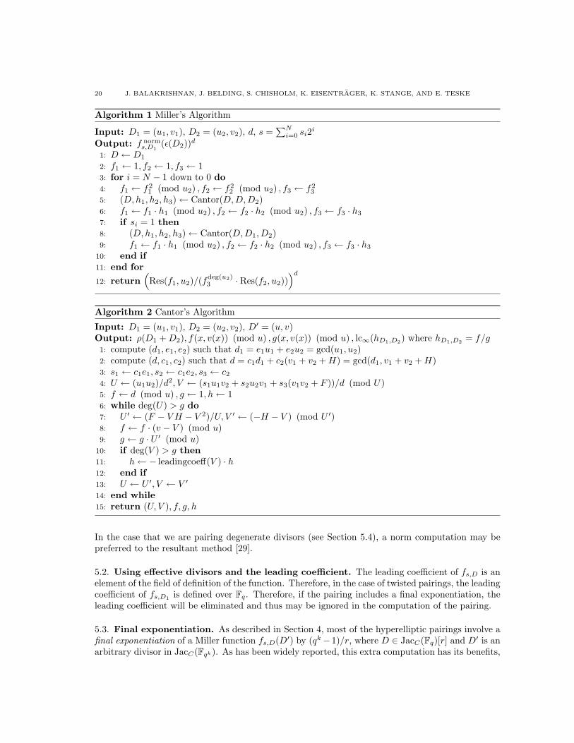
5.1. Miller’s algorithm. The algorithm used to compute Weil and Tate-Lichtenbaum pairings onelliptic curves was devised by Victor Miller in 1985 [58] and can be adapted to all pairings discussedin this paper [15]. Referring to the pairing definitions of Section 4 one sees that to compute apairing, it is necessary to evaluate a Miller function at a divisor. Algorithm 1, futheron referred toas “Miller’s algorithm”, computes such a value using the structure of an addition chain for s.

Usually, an addition chain takes the form of a double-and-add chain, as follows. Starting with theinteger k = 0, at each step one performs one of two possible calculations to update the value of k:one either doubles to obtain k → 2k or doubles-and-adds to obtain k → 2k + 1. To determine thesequence of steps needed to obtain any desired integer s in this way, one reads the binary digits ofs from left to right, doubling once for each ‘0’ and doubling-and-adding for each ‘1.’ (For example,5 = 1012 is obtained as 0 → 2(0) + 1 = 1 → 2(1) = 2 → 2(2) + 1 = 5.) Starting from 0, thisalgorithm computes s in blog2 sc+ 1 steps (each of which consists of either one or two additions).

Miller’s Algorithm computes fs,D following this double-and-add process by computing the Millerfunction fk,D at each step along the way, obtaining fs,D at the end. A double step involves oneaddition, and a double-and-add step involves two. For each addition, we compute the new Millerfunction fi+j,D from the previously computed fi,D and fj,D via the relationship

fi+j,D = fi,Dfj,DhiD,jD, i, j > 0,

where the auxiliary function hD′,D′′ is a function with divisor

ρ(D′) + ρ(D′′)− ρ(D′ +D′′).

The computation of hD′,D′′ is performed by an enhanced version of Cantor’s Algorithm (cf. Section2.3), here Algorithm 2. It is called under the name Cantor() once (if doubling) or twice (if doublingand adding) in each for-loop of Miller’s Algorithm. Using the result of Algorithm 2, one calculates


f2i,D from fi,D (“double”) or f2i+1,D from fi,D and f1,D (“double and add”), where f1,D is a constantfunction.

In order to compute the pairing value, the Miller function fs,D2 must be evaluated a divisor D1, butthis evaluation is not possible unless D1 and D2 have disjoint support, which is not the case if bothare reduced. However, using reduced divisors and Mumford representation is too useful to dispensewith, so the solution is the following. Let z be a uniformizer at P∞ (for example, z(x, y) = x2/y isa convenient choice). Then, if f is a function with order −r at P∞, define the leading coefficient atP∞ of f , denoted as lc∞(f), to be (zrf)(P∞). Then the normalization of f is the scalar multiplef norm = f/lc∞(f) which has leading coefficient 1. For the hyperelliptic Ate pairing [36, Lemma 6],when z is Fq-rational,

fq,ρ(D2)(D1) = f normq,ρ(D2)

(ε(D1)).

The right-hand expression requires computing the leading coefficient, but solves the problem ofnon-disjoint supports of D1 and D2 without losing the usefulness of Mumford representation.

For HV Pairings and the modified Tate-Lichtenbaum pairing, the same solution is possible. Considerthe computation of t(D2, D1) = fr,D2(D1)(q

k−1)/r where D1, D2 are reduced. Let −bi be the coeffi-cient of P∞ in Di for i = 1, 2. (Note that bi = −1 or −2, depending on whether or not the reduceddivisor Di is degenerate.) The function fr,D2 has divisor rD2 with order −b2r at P∞. Therefore, ifz is an Fqk -rational uniformizer at P∞,

fr,D2(D1) = f normr,D2

(ε(D1))/z(P∞)b1b2r.

Since b1b2r is a multiple of r, the contribution of z(P∞)b1b2r(qk−1)/r is 1, and thus

fr,D2(D1)(qk−1)/r = f norm

r,D2(ε(D1))(q

k−1)/r.

As the HV pairing as,h(D2, D1) is a simply a power of the modified Tate pairing t(D2, D1) (see The-orem 4.1), in whichever form the pairing as,h(D2, D1) is computed, evaluating normalized functionsat effective divisors will give the pairing value.

In the elliptic curve case, it is more efficient to evaluate the Miller functions and the auxiliaryfunctions hD′,D′′ at the desired divisor (denoted D2 in Miller’s Algorithm) at each step, instead ofreserving the evaluation for the end. In order to allow for this, D2 is passed to Cantor’s Algorithm.We now turn to a discussion of this aspect in the case of hyperelliptic curves.

In Miller’s Algorithm, the current Miller function f is stored as two polynomials f1 and f2 suchthat f = f1/f2. Similarly, the auxiliary functions h are returned from Cantor’s Algorithm as h1

and h2. It remains to explain how to evaluate a polynomial function g(x, y) on C at the effectivepart of a divisor given in Mumford representation (u(x), v(x)) (we need only the effective partbecause of the preceeding discussion and the computation of the leading coefficient). We need toevaluate G(x) = g(x, v(x)) at the zeroes of u(x). This is the same as computing the resultantRes(G(x), u(x)). Performing a resultant calculation is sufficiently costly that it is best left to theend of Miller’s Algorithm, as long as the size of the Miller functions can be kept low in the meantime.Fortunately, in preparation for the eventual final resultant, it suffices to compute the Miller functionsin x and y modulo u(x), while substituting y = v(x), effectively capping their degrees.

If Steps 5 and 8 through 13 are removed from Cantor’s Algorithm and only (U, V ) is returned, thealgorithm computes ρ(D1 +D2) for any divisors D1 and D2 in Mumford representation (this is theusual meaning of “Cantor’s Algorithm” as in Section 2.3). If these steps are included, then Cantor’sAlgorithm can also return f, g (mod u) such that f/g = hD1,D2(x, v(x)) for some specified divisor(u, v). This is the form in which it is used in Miller’s Algorithm.


Algorithm 1 Miller’s Algorithm

Input: D1 = (u1, v1), D2 = (u2, v2), d, s =∑N

i=0 si2i

Output: f norms,D1

(ε(D2))d

1: D ← D1

2: f1 ← 1, f2 ← 1, f3 ← 13: for i = N − 1 down to 0 do4: f1 ← f2

1 (mod u2) , f2 ← f22 (mod u2) , f3 ← f2

3

5: (D,h1, h2, h3)← Cantor(D,D,D2)6: f1 ← f1 · h1 (mod u2) , f2 ← f2 · h2 (mod u2) , f3 ← f3 · h3

7: if si = 1 then8: (D,h1, h2, h3)← Cantor(D,D1, D2)9: f1 ← f1 · h1 (mod u2) , f2 ← f2 · h2 (mod u2) , f3 ← f3 · h3

10: end if11: end for12: return

(Res(f1, u2)/(f

deg(u2)3 · Res(f2, u2))

)d

Algorithm 2 Cantor’s Algorithm

Input: D1 = (u1, v1), D2 = (u2, v2), D′ = (u, v)Output: ρ(D1 +D2), f(x, v(x)) (mod u) , g(x, v(x)) (mod u) , lc∞(hD1,D2) where hD1,D2 = f/g1: compute (d1, e1, e2) such that d1 = e1u1 + e2u2 = gcd(u1, u2)2: compute (d, c1, c2) such that d = c1d1 + c2(v1 + v2 +H) = gcd(d1, v1 + v2 +H)3: s1 ← c1e1, s2 ← c1e2, s3 ← c24: U ← (u1u2)/d2, V ← (s1u1v2 + s2u2v1 + s3(v1v2 + F ))/d (mod U)5: f ← d (mod u) , g ← 1, h← 16: while deg(U) > g do7: U ′ ← (F − V H − V 2)/U, V ′ ← (−H − V ) (mod U ′)8: f ← f · (v − V ) (mod u)9: g ← g · U ′ (mod u)

10: if deg(V ) > g then11: h← − leadingcoeff(V ) · h12: end if13: U ← U ′, V ← V ′

14: end while15: return (U, V ), f, g, h

In the case that we are pairing degenerate divisors (see Section 5.4), a norm computation may bepreferred to the resultant method [29].

5.2. Using effective divisors and the leading coefficient. The leading coefficient of fs,D is anelement of the field of definition of the function. Therefore, in the case of twisted pairings, the leadingcoefficient of fs,D1 is defined over Fq. Therefore, if the pairing includes a final exponentiation, theleading coefficient will be eliminated and thus may be ignored in the computation of the pairing.

5.3. Final exponentiation. As described in Section 4, most of the hyperelliptic pairings involve afinal exponentiation of a Miller function fs,D(D′) by (qk−1)/r, where D ∈ JacC(Fq)[r] and D′ is anarbitrary divisor in JacC(Fqk). As has been widely reported, this extra computation has its benefits,


in particular when k is even. Many of these are described by Scott [68] and Galbraith, Hess, andVercauteren [29]; we summarize the main ones here.

When k is even, the field Fqk can be constructed as a degree two extension of Fq` , where 2` = k.We can represent elements as a + ib with a, b ∈ Fq` and γ2 a quadratic non-residue over Fq` . It isstraightforward to check that

(1/(a+ γb))q`−1 = (a− γb)q`−1

which means inversion can be replaced by conjugation since the result is the same after final expo-nentiation. In particular, this applies to any denominators of computations in Miller’s algorithm.

There is a further optimization, denominator elimination, which in fact allows one to ignore alldenominators in Miller’s algorithm. In computing fs,D(D′) where D is a divisor defined over thebase field Fq, one computes the numerator and denominator values separately (see Algorithm 1). IfD′ = (u(x), v(x)) has u(x) defined over Fq` , then the computation of the denominator involves onlyD and u(x) and therefore becomes trivial after final exponentiation. In the case of supersingularcurves, for example, a suitable evaluation divisor can be found using a distortion map ψ (see Section4.7) such that ψ(D′) has x-coordinates in Fq` [33].

The final exponentiation is generally computed in multiple steps by writing (qk−1)/r as a product ofpolynomials in base q expansion and exploiting finite field constructions, in particular the qth powerof Frobenius, which speeds up computation [29]. Other methods for faster computation includesigned sliding window methods [37], as well as trace and tori methods [34, 38].

Remark 5.1. As the Ate pairing does not require final exponentiation, these techniques are un-available. Furthermore, as stated by Granger et al., there are also possible security implications;namely, the problem of pairing inversion (given γ and D1, find D2 such that a(D1, D2) = γ) may notbe as hard (see [36, Intro.]). However, we remark that if r2 - (qk − 1) and r is prime, a superfluousfinal exponentiation of the Ate pairing still gives a non-degenerate result.

5.4. Degenerate divisors. For a genus 2 curve, a general reduced divisor D is of the form D =(P1) + (P2) − 2(∞) and a degenerate divisor is of the form D = (P ) − (∞). As there are fewerpoints in the support, the arithmetic is faster when adding a general divisor to a degenerate divisorthan when adding two general divisors. This speeds up the computation of the Miller function fs,D

where D is degenerate. Furthermore, the evaluation of a Miller function on a degenerate divisor isalso faster by at least half, since there is only one affine point. Many of the fastest hyperellipticpairing computations use degenerate divisors, including the examples noted with [a], [b] and [c] inthe Table 5.6. We summarize here when it is possible to use degenerate divisors as either the firstor second argument of a pairing.

Should JacC(Fq) be of prime order r, then for any P ∈ C(Fq), the divisor D = (P ) − (∞) can beused as the first argument, regardless of the pairing. Furthermore, if C is supersingular, then using adistortion map ψ (see Section 4.7), we have that ψ(D) is also degenerate and pairs non-trivially withD. Hence, for supersingular curves with prime-order JacC(Fq), we can use degenerate divisors asboth arguments of the Tate-Lichtenbaum pairing. This fact was originally exploited in the definitionof the ηT pairing by Duursma and Lee [14]. In the more general situation where #JacC(Fq) is notprime and/or the curve C is not supersingular, using degenerate divisors is not as straightforward,as noted by Frey and Lange [24]. If #JacC(Fq) = nr where gcd(n, r) = 1, there is no guarantee thatthere exists a degenerate divisor D of order r. The probability that a reduced divisor is of orderr is 1/n and the probability that a divisor is degenerate is roughly 1/q, by the Hasse-Weil boundson C(Fq) and JacC(Fq). Therefore, assuming independence, a heuristic argument gives that the


probability a divisor is degenerate and order r is 1/qn. This implies that using a degenerate divisorfor the first argument is not necessarily possible.

However, Frey and Lange [24] show that for q large enough (as in a cryptographic setting), itis possible to use a degenerate divisor as the second argument. In other words, there exists D2 =(P )−(∞) ∈ JacC(Fqk) such that for any D1 ∈ JacC(Fq)[r], the Tate-Lichtenbaum pairing τ(D1, D2)is non-trivial. The probability that P ∈ C(Fqk) yields such a divisor D2 has a lower bound of1/k log2 q. Moreover, if k = 2d is even, it is possible to choose P = (x, y) with x ∈ Fqd and y ∈ Fqk ,using a degenerate divisor on the quadratic twist of C/Fqd . This technique is used for example byFan, Gong and Jao [16] and allows for denominator elimination.

Remark 5.2. As remarked by Galbraith, Hess and Vercauteren [29, §7], there are potential secu-rity implications with using degenerate divisors, depending on the application. While the discretelogarithm problem with a degenerate divisor as a base point is no easier than that with a generaldivisor [44], other hardness assumptions such as pairing inversion (see Remark 5.1) are potentiallycompromised, as Granger et al. have noted [36]. To our knowledge, the topic remains unresolved.

We also remark that there are protocols in which it may not always be possible to use degeneratedivisors, for example, when computing a pairing where one input is required to be a random multipleof a divisor D.

5.5. Rubin-Silverberg point compression. Another method available to us in genus 2 is thepoint compression technique of Rubin and Silverberg [66], who note that supersingular abelianvarieties can be identified with subvarieties of Weil restrictions of supersingular elliptic curves.

Recall that a supersingular q-Weil number is a complex number of the form√qζ, where ζ is a root

of unity and√q denotes the positive square root. Let m be the order of ζ.

The following theorem allows us to define a useful invariant:

Theorem 5.3 ([66]). Suppose A is a simple supersingular abelian variety of dimension g overFq, where q is a power of a prime p, and P (x) is the characteristic polynomial of the Frobeniusendomorphism of A. Then P (x) = G(x)e, where G(x) ∈ Z[x] is a monic irreducible polynomial withe = 1 or 2. All of the roots of G are supersingular q-Weil numbers.

We call the roots of G the q-Weil numbers for A.

Definition 5.4. The cryptographic exponent of A is defined by

cA =

m

2, if q is a square

m

gcd(2,m), if q is not a square.

Let αA = cA/g; it is the security parameter of A.

Now let F ⊂ F′ be finite fields, E an elliptic curve over F, and let Q ∈ E(F′). Recall that the tracefrom F′ to F is given by

TrF′/F(Q) =∑

σ∈Gal(F′/F)

σ(Q).

Rubin and Silverberg prove the following result:


Theorem 5.5 ([66]). Let E be a supersingular elliptic curve over Fq, π a q-Weil number for E(π 6∈ Q). Fix r ∈ N with gcd(r, 2pcE) = 1. Then there is a simple supersingular abelian variety Aover Fq having the following properties.

(1) dimA = ϕ(r).(2) For every primitive rth root of unity ζ, πζ is a q-Weil number for A.(3) cA = rcE.(4) αA = (r/φ(r))αE.(5) There is a natural identification of A(Fq) with the following subgroup of E(Fqr ) :

{Q ∈ E(Fqr ) : TrFqr /Fqr/l

(Q) = 0 for every prime l | r}.

This theorem can be thought of as a form of point compression for supersingular elliptic curves.More concretely, the theorem allows us to replace the Jacobian of a hyperelliptic curve C over Fwith an elliptic curve E over an extension F′ of F, while still exploiting the per-bit security gain ofhigher genus hyperelliptic curves. From a security standpoint, there is no difference between workingwith E(F′) and working with JacC(F). On the other hand, one needs fewer bits to represent divisorswith support in C(F) than to represent points in E(F′).

As noted by Galbraith [28], recent implementations [2] indicate that pairings on elliptic curveswith the Rubin-Silverberg compression are, in general, more efficient than using the pairings onJacobians of hyperelliptic curves. However, it seems that Rubin and Silverberg have initiated apromising investigation into the arithmetic geometry of abelian varieties and its applications topairings. Much work remains to be done, in particular with respect to the torsion structure of thesevarieties.

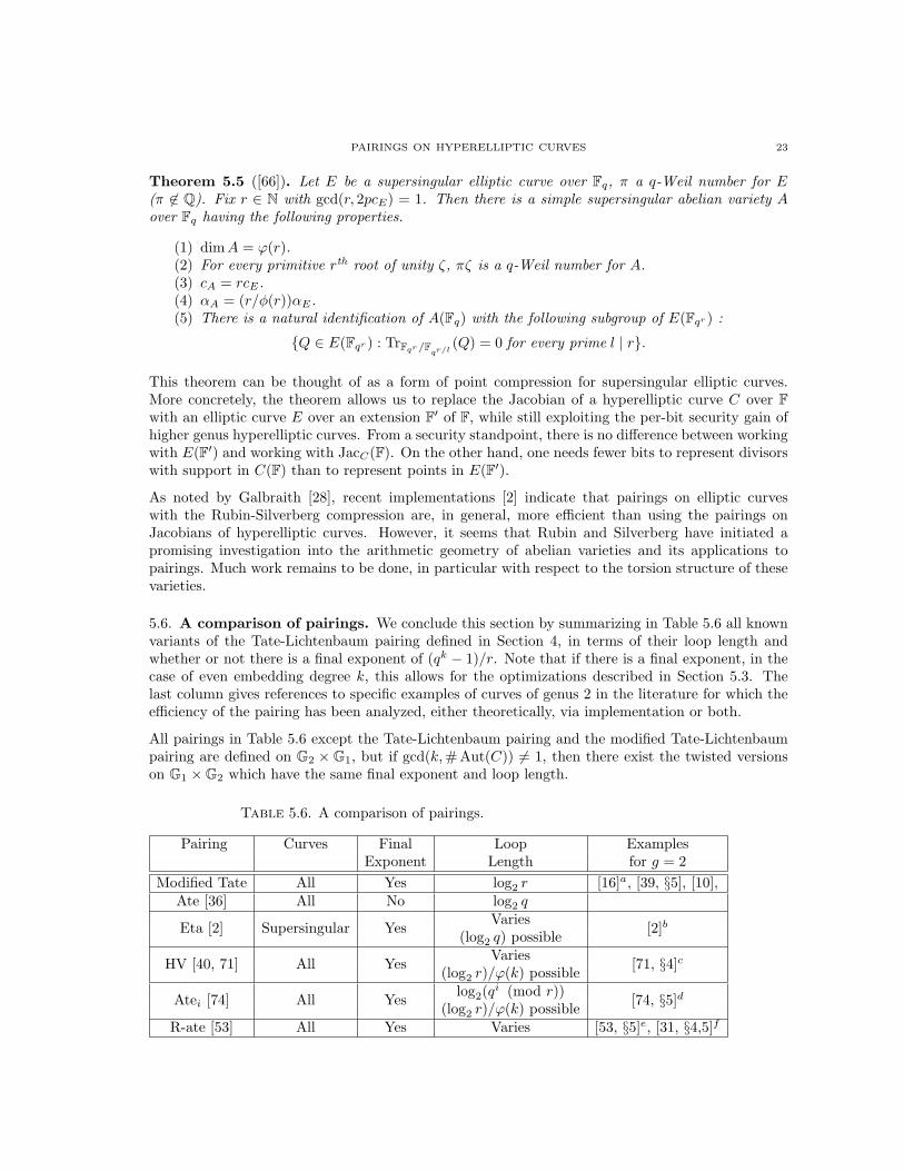
5.6. A comparison of pairings. We conclude this section by summarizing in Table 5.6 all knownvariants of the Tate-Lichtenbaum pairing defined in Section 4, in terms of their loop length andwhether or not there is a final exponent of (qk − 1)/r. Note that if there is a final exponent, in thecase of even embedding degree k, this allows for the optimizations described in Section 5.3. Thelast column gives references to specific examples of curves of genus 2 in the literature for which theefficiency of the pairing has been analyzed, either theoretically, via implementation or both.

All pairings in Table 5.6 except the Tate-Lichtenbaum pairing and the modified Tate-Lichtenbaumpairing are defined on G2 × G1, but if gcd(k,# Aut(C)) 6= 1, then there exist the twisted versionson G1 ×G2 which have the same final exponent and loop length.

Table 5.6. A comparison of pairings.

Pairing Curves Final Loop ExamplesExponent Length for g = 2

Modified Tate All Yes log2 r [16]a, [39, §5], [10],Ate [36] All No log2 q

Eta [2] Supersingular Yes Varies [2]b(log2 q) possible

HV [40, 71] All Yes Varies [71, §4]c(log2 r)/ϕ(k) possible

Atei [74] All Yes log2(qi (mod r)) [74, §5]d(log2 r)/ϕ(k) possibleR-ate [53] All Yes Varies [53, §5]e, [31, §4,5]f


[a] Fan, Gong and Jao use efficiently computable automorphisms to compute a power of themodified Tate-Lichtenbaum pairing on two Kawazoe-Takahashi families of non-supersingularcurves over prime fields. This algorithm allows for a theoretical reduction of up to one fourthin the length of the Miller loop (log2 r). They implement this on curves over Fp where p isa 329-bit prime and k = 4 and compare this with pairings on a supersingular curve definedover Fp with p a 256-bit prime and k = 4. Using all known optimizations (degenerate divi-sors, encapsulated group operations, final exponentiation, fast field arithmetic), the pairingcomputation on the non-supersingular curve is about 55.8% faster.

[b] This is one of the fastest known pairing implementations on a hyperelliptic curve and makesuse of many optimizations including degenerate divisors and a special octupling formula.

[c] Vercauteren gives an example of a family of supersingular curves with k = 12 such thatthe loop length is approximately log2 r/ϕ(k).

[d] Zhang gives examples of Kawazoe-Takahashi curves with k = 8, 24 such that the twistedAtei pairing has loop length approximately log2 r/ϕ(k).

[e] Lee, Lee and Park show that for supersingular curves the loop length can theoreticallybe approximately (log2 q)/2. They also compute an example on a Duursma-Lee curve withk = 5, achieving a loop length 21% shorter than the Ate.

[f ] Galbraith, Lin and Mireles Morales [31] describe how to use the R-ate pairing on a realmodel of a hyperelliptic curve of genus 2 over Fp with k = 6. By using a distortion mapψ on JacC(Fp)[r] such that the image of G1 is in the p-eigenspace, G2, they are also ableto make use of denominator elimination. They conclude that such pairings are theoreticallycompetitive with both pairings on certain elliptic curves with k = 3 and with hyperellipticcurves in the imaginary model with k = 4.

6. Future Work on Hyperelliptic Pairings

In this section, we present possible areas for future work, expanding upon the list in the 2007 surveypaper of Galbraith, Hess and Vercauteren [29]. We list some newer problems, mention some recentadvancements in the elliptic curve case which may find generalizations in pairings for g ≥ 2, andconclude by revisiting the 2007 list [29].

6.1. Achieving optimal loop length. Since 2007, there has been a flurry of new work to reducethe loop length in Miller’s algorithm using variants of the Ate pairing. In particular, the Ate pairingon hyperelliptic curves of genus g already reduces the loop length by up to a factor of g whencompared to the Tate-Lichtenbaum pairing [36]. Vercauteren [71] uses the following definition tocharacterize pairings with certain loop lengths.

Definition 6.1. [71] Let e : G1 × G2 7→ µr ⊂ F∗qk be a non-degenerate, bilinear pairing definedusing a combination of Miller functions. We call e(·, ·) an optimal pairing if it can be computedusing (log2 r)/ϕ(k) + ε(k) Miller iterations, where ϕ is the Euler phi function and ε(k) ≤ log2 k.

Note that this means a pairing is optimal if the total sum of all the loop lengths of the Millerfunctions is approximately (log2 r)/ϕ(k).

For an HV pairing as,h(x) with h(x) =∑n

i=0 hixi, the total sum of loop lengths is

∑ni=0 log2 hi. Thus

to be optimal, it is necessary but not sufficient that the coefficients of h are bounded by rϕ(k). Thiscan be achieved by finding the shortest vectors in a lattice spanned by vectors involving powers of s[71, §3.3]. Vercauteren and Zhang both give examples of genus 2 HV pairings (see Table 5.6) wherethe polynomial h(x) satisfies this bound and has only one coefficient which is not ±1, therefore


providing examples of optimal hyperelliptic pairings. It remains open whether given a hyperellipticcurve it is always possible to construct an optimal HV pairing. One direction would be to lookat extending the method of Vercauteren [71] which constructs optimal pairings on parameterizedfamilies of elliptic curves.

Vercauteren also conjectures that for elliptic curves without efficiently computable automorphismsother than the Frobenius, no pairing can be better than optimal [71, §2]. More specifically, heconjectures that for such a curve, any non-degenerate pairing requires at least (1 − δ) log2 r/ϕ(k)Miller iterations where 0 < δ < 1/4. For a curve with a set of efficiently computable endomor-phisms E ⊂ End(E), Vercauteren defines a superoptimal pairing as one which can be computed using(log2 r)/#E + ε(k) Miller iterations. It remains to examine what is the best possible for genus 2curves, both with and without the existence of efficiently computable endomorphisms (see also Sec-tion 6.2). Furthermore, it is not known whether there are other non-degenerate, bilinear hyperellipticpairings on G1 ×G2 which are not part of the HV framework.

Lastly, we remark that the computation of an HV pairing cannot be measured solely by the sumof loop lengths. There is also the cost of computing the auxiliary functions (see (2),(3) in Section4.6). It remains to formally compare the cost of these additional computations with the benefit ofa shorter total sum of Miller loop lengths.

6.2. Using efficiently computable automorphisms. One newer method to speed up computa-tions is to use efficiently computable automorphisms of the curve C (beyond the Frobenius). Forexample, Fan, Gong and Jao use efficiently computable automorphisms in computing a power of themodified Tate-Lichtenbaum pairing on some specific non-supersingular genus 2 curves over primefields [16]. An open task is to explore how far can this be generalized to other genus 2 curves.

Furthermore, Hess [40] extends his pairing framework for ordinary elliptic curves to exploit efficientlycomputable automorphisms. This does not generally give an improved loop length since #E ≤ ϕ(k)for most ordinary elliptic curves. However, as hyperelliptic curves have a greater variety of Aut(C),it would be worthwhile to examine what improvements in loop length can be made by extending theHV framework to exploit these automorphisms.

6.3. Fast arithmetic and the embedding degree. In the case of even embedding degree k, itis traditional to exploit the degree two subfield, as explained in Section 5.3. In fact, Koblitz andMenezes define pairing friendly fields to be finite fields of the form Fqk such that k = 2i3j for0 ≤ i, j ∈ Z and q ≡ 1 (mod 12) [48, §5]. (If k is strictly a power of 2 then it is only required thatq ≡ 1 (mod 4) .) By a theorem of Lidl and Niederreiter [56, Theoreom 3.75] and more particularly, bya specific instance of this theorem given by Koblitz and Menezes [48, Theorem 2], we can constructthe extension Fqk for k of this form using a tower of quadratic and cubic extensions. There are thuscertain advantages we can make use of for k = 2i3j . For instance, there exist fast arithmetic methodsfor degree 2 and 3 subextensions; namely, the Karatsuba method for quadratic subextensions and theToom-Cook method for cubic subextensions [46, §4.3.3]. These methods are used to economize thearithmetic in the smaller fields which reduce the number of field multiplications. However, there areembedding degrees not of this form, particularly among recent constructions of non-supersingularcurves, and hence it would be worthwhile to see if these ideas can be extended to embedding degreesk containing other prime factors.


6.4. Degenerate divisors. As discussed in Section 5.4, one common optimization is to use degen-erate divisors. Frey and Lange [24] give a lower bound on the probability that P ∈ C(Fqk) givesa non-trivial pairing value when used as a degenerate divisor in the second argument of the Tate-Lichtenbaum pairing. However, to our knowledge, there is no method to efficiently find such pointsbeyond simple trial and error.

We also consider using degenerate divisors with Ate-type pairings a on G2 ×G1 (or twisted Ate onG1 × G2). While a heuristic argument shows that the likelihood that a divisor of G1 is degenerateis small, it would be useful to know if there are particular curves where this is more likely and ifso, how to find such divisors. It also remains to analyze the likelihood that an element of G2 isdegenerate. We note that for D ∈ G2, if D = (P ) − (∞), then π(D) = (π(P )) − (∞) implies thatthe divisor class qD is also degenerate.

6.5. Ignoring the last bit. In the case of the modified Tate-Lichtenbaum pairing on elliptic curves,when computing fr,D1(D2), it is possible to ignore the last bit in the expansion of r. This followsfrom the fact that since r is odd, the last iteration of the Miller loop of the Tate-Lichtenbaum pairingis the evaluation at D2 of the line function corresponding to the line through (r−1)P and P . This isa vertical line and so by the choice of divisor D2 with x-coordinates lying over Fqd , this is eliminatedby the final exponentiation. While this does not give a large improvement compared to other looplength reductions, it is worth verifying whether this trick might be used in the case of hyperellipticcurves.

6.6. Compression and higher degree twists. Galbraith and Lin [30] give explicit formula tocompute the Weil pairing on elliptic curves given only x-coordinates, and the Tate-Lichtenbaum andAte pairings given both x-coordinates but at most one y-coordinate. This form of point compressionis advantageous for elliptic curve pairings with small embedding degree, where one would be workingover a field of large order (and consequently, taking a square root to recover y could be expensive).The compression makes use of explicit recurrence formulas for elliptic curve point multiplication andfor Miller functions in the case of embedding degree k = 2. As these recurrences are given solely interms of the x-coordinate of the point, the pairings are also computed in terms of the x-coordinateof the points involved. Note, however, that neglecting the value of y introduces a sign ambiguity,but this is resolved by taking the trace of the pairing, which is independent of the sign of y. It isperhaps worth investigating if the analogous results may be obtained for hyperelliptic pairings (forcurves of the form y2 = F (x)) of small embedding degree.

Another form of compression involves algebraic tori, which are d-dimensional generalizations ofthe multiplicative group Gm. Naehrig, Barreto and Schwabe [60] use algebraic tori to compresscomputations, not just in the final exponentiation but also in the Miller loop of elliptic curve pairings.Their methods rely on explicit formulas for multiplication and squaring of torus elements and alsoexploit degree 6 twists. One might want to try similar methods for certain twists of hyperellipticcurves.

Another benefit of twists, as explained in Section 4.7, is that curves with a twist of degree d allowone to use the twisted versions of Ate-type pairings. This means one computes the Miller functionfs,D1(D2) for D1 ∈ G1 and the divisor D2 = (u(x), v(x)) ∈ G2 with u(x) defined over the subfieldFqk/(d,k) , as opposed to computing fs,D2(D1). Furthermore, the points of G2 can be represented aspoints on the Jacobian of the twist C ′ which allows for faster computations in the group G2. Theexample of Zhang [74] uses a twist of degree 8; to our knowledge, pairings on curves with twists ofdegree 10 have not been implemented.


6.7. Trace zero subvarieties. For a hyperelliptic curve C of genus g defined over Fq, a tracezero subvariety of C is a subgroup of the Jacobian of C whose construction is connected to theWeil restriction of scalars. The use of trace zero varieties for cryptographic applications was firstsuggested by Frey [23]. The trace zero subvariety of C over a field extension of degree ` is a subgroupof JacC(Fq`), which is isomorphic to the quotient JacC(Fq`)/JacC(Fq).

It can also be defined concretely as follows: Let π be the qth power Frobenius. Let ` be a primeand assume that ` - #JacC(Fq). We define the trace zero subvariety G` of JacC(Fq`) to be the setof elements of trace zero. I.e.,

G`(Fq) := {D ∈ JacC(Fq`) : D + π(D) + · · ·+ π`−1(D) = O}.Since G`(Fq) is the kernel of the trace map, it is a subgroup of JacC(Fq`). To perform arithmeticin a trace zero subvariety one can use the algorithms that work in the whole Jacobian. So far, nospecific algorithms for the group law are known that make use of the subgroup properties.

Since G`(Fq) is a subgroup of JacC(Fq`), we can define a Tate-Lichtenbaum pairing on it by re-striction: suppose the order of G`(Fq) is divisible by a large prime factor r, but not by r2. LetG1 := G`[r] ∩ ker(π` − [1]) and G2 := G`[r] ∩ ker(π` − [q`]). Then the Tate-Lichtenbaum pairing onG` is a map

t : G1 ×G2 → µr.

On the points of G1, π acts as multiplication by an integer s ([13]), and the same is true for theaction of π on G2 ([9, Proposition 3]). Cesena [9] gives a new algorithm for computing the Tate-Lichtenbaum pairing over trace zero subvarieties of supersingular elliptic curves by exploiting theaction of the q-Frobenius. He uses the fact that the q-Frobenius π is an efficient endomorphism(rather than just the qr-Frobenius), together with the fact that for particular supersingular ellipticcurves the action of the Frobenius can be computed more efficiently [9, Lemmas 1–3]. For thesecurves, the action of π is (close to being) multiplication of a power of q.

Experimentally, Cesena’s algorithm is as efficient as the Tate-Lichtenbaum pairing on supersingularelliptic curves, though less efficient than the eta pairing ηT or the optimal Ate pairing of Vercauteren.It remains to explore whether Cesena’s algorithm generalizes to supersingular hyperelliptic curvesor non-supersingular trace zero varieties.

6.8. Exploiting torsion groups of dimension > 2. If r is coprime with the characteristic ofFq, the r-torsion group of a Jacobian variety of dimension g is isomorphic to (Z/rZ)2g. With theexception of the recent work by Okamoto and Takashima [63], all known pairing-based cryptographicapplications require only two linearly independent torsion points and thus can be realized in theelliptic curve setting; in fact, also the Okamoto-Takashima protocols can as well be implementedusing a product of two (supersingular) elliptic curves. It is an open problem to find a cryptographicapplication that uses curves of genus 2 (or larger) and that does not work using elliptic curves. Bothfor the ordinary and the supersingular case, constructions of Jacobians of dimension 2 with low fullembedding degree (cf. Section 3.3) are available ([18, 63]).

6.9. More Problems. For completeness, we include the problems posed by Galbraith, Hess andVercauteren [29], making note of any recent advancements:

(1) Construct pairing-friendly ordinary hyperelliptic curves with smaller ρ-values. At this pointin time, the smallest ρ-value obtained for an ordinary hyperelliptic curve of small embeddingdegree is ρ ≈ 20/9 (for g = 2, k = 27; cf. Section 3). It is highly desirable to have curveswith ρ-value < 2.


(2) Curves with g ≥ 3. For curves with g ≥ 3, is it possible to develop efficient pairing-basedcryptosystems which are also secure against the index calculus attacks available for thesecurves?

(3) Pairings on real models of hyperelliptic curves. There have been recent examples [31] ofefficient pairing computations on real models of hyperelliptic curves, as remarked in Section5.6. Are real models competitive with the imaginary models in general? Furthermore, arethere efficient pairings on non-hyperelliptic curves?

(4) Torsion structure. Is there an efficient method for selecting divisors from JacC(Fqk)[r] forpairing computations? (See also Section 6.4.) Furthermore, if this group has more than twogenerators, what cryptographic applications are possible? (See also Section 6.8.)

(5) Rubin-Silverberg point compression and Weil restriction. Can the Rubin-Silverberg method(see Section 5.5) be made more efficient in the elliptic curve case and/or generalized toJacobians of curves of genus g ≥ 2?

(6) Weil restriction. As in Rubin-Silverberg point compression, certain abelian varieties can beidentified with subvarieties of the Weil restriction of supersingular elliptic curves. When theabelian variety is a Jacobian, are there explicitly computable homomorphisms between theelliptic curve and the Jacobian representation?

Acknowledgments. The authors are most grateful to David Freeman for his elaborate feedbackon earlier versions of this paper, which significantly improved our work. The authors further thankPaulo S.L.M. Barreto, Anja Becker, Felix Fontein, Steven Galbraith, and Alfred Menezes for helpfuldiscussions and comments on an earlier draft of the paper. Thanks to Alan Silvester for conscientioustechnical editing. Thanks to Jonathan Wise. The work of the first author has been supported by aNational Science Foundation Graduate Research Fellowship. The third author has been supportedby the Informatics Circle of Research Excellence Chair in Algorithmic Number Theory and Cryptog-raphy. The fourth author is partially supported by National Science Foundation grant DMS-0801123and a Sloan Research Fellowship. The work of the fifth author has been supported by a NationalScience Foundation Fellowship (#0802915) and a National Science and Engineering Research Coun-cil Fellowship (#373333). The fifth author is also grateful to Harvard University and the PacificInstitute for the Mathematical Sciences UBC, where some of this work was conducted. Lastly, thesixth author acknowledges support by the National Science and Engineering Research Council ofCanada, and by the Premier’s Research Excellence Award of the province of Ontario.

The idea for this paper was conceived during the workshop “Women in Numbers” at the BanffInternational Research Station in November 2008, where the authors formed a project group studyinghyperelliptic pairings.

References

1. R. Balasubramanian and N. Koblitz, The improbability that an elliptic curve has subexponential discrete logproblem under the Menezes-Okamoto-Vanstone algorithm, Journal of Cryptology 11 (1998), no. 2, 141–145.

2. P.S.L.M. Barreto, S. Galbraith, C. O hEigeartaigh, and M. Scott, Efficient pairing computation on supersingularabelian varieties, Designs, Codes and Cryptography 42 (2007), 239–271.

3. D. Boneh and M. Franklin, Identity-based encryption from the Weil pairing, SIAM Journal on Computing 32(2003), no. 3, 586–615.

4. D. Boneh, B. Lynn, and H. Shacham, Short signatures from the Weil pairing, Journal of Cryptology 17 (2004),no. 4, 297–319.

5. F. Brezing and A. Weng, Elliptic curves suitable for pairing based cryptography, Designs, Codes and Cryptography37 (2005), 133–141.

6. D. Cantor, Computing in the Jacobian of a hyperelliptic curve, Mathematics of Computation 48 (1987), no. 177,95–101.


7. G. Cardona, On the number of curves of genus 2 over a finite field, Finite Fields and Their Applications 9 (2003),no. 4, 505–526.

8. G. Cardona, E. Nart, and J. Pujolas, Curves of genus two over fields of even characteristic, MathematischeZeitschrift 250 (2005), no. 1, 177–201.

9. E. Cesena, Pairing with supersingular trace zero varieties revisited, Cryptology ePrint Archive Report 2008/404,http://eprint.iacr.org/2008/404/.

10. Y.-J. Choie and E. Lee, Implementation of Tate pairing on hyperelliptic curves of genus 2, ICISC 2003, LNCS,vol. 2971, Springer-Verlag, 2004, pp. 97–111.

11. C. Cocks and R.G.E. Pinch, Identity-based cryptosystems based on the Weil pairing, unpublished manuscript,2001.

12. D. Coppersmith, Fast evaluation of logarithms in fields of characteristic two, IEEE Transactions on InformationTheory 30 (1984), 587–594.

13. D. Doche and T. Lange, Handbook of Elliptic and Hyperelliptic Curve Cryptography, ch. 15 (Arithmetic of specialcurves), Chapman & Hall/CRC, 2006.

14. I. Duursma and H.-S. Lee, Tate pairing implementation for hyperelliptic curves y2 = xp − x + d, Advances inCryptology - Asiacrypt 2003, LNCS, vol. 2894, Springer-Verlag, 2003, pp. 111–123.

15. K. Eisentrager, K. Lauter, and P. Montgomery, Improved Weil and Tate pairings for elliptic and hyperellipticcurves, Algorithmic Number Theory ANTS-VI, LNCS, vol. 3076, Springer-Verlag, 2004, pp. 169–183.

16. X. Fan, G. Gong, and D. Jao, Speeding up pairing computations on genus 2 hyperelliptic curves with efficientlycomputable automorphisms, Pairing 2008, LNCS, vol. 5209, Springer-Verlag, 2008, pp. 243–264.

17. D. Freeman, A generalized Brezing-Weng method for constructing pairing-friendly ordinary abelian varieties:Additional examples, http://theory.stanford.edu/∼dfreeman/papers/gen-bw-examples.pdf.

18. , Constructing pairing-friendly genus 2 curves with ordinary Jacobians, Pairing 2007, LNCS, vol. 4575,Springer-Verlag, 2007, pp. 152–176.

19. , A generalized Brezing-Weng algorithm for constructing pairing-friendly ordinary abelian varieties, Pair-ing 2008, LNCS, vol. 5209, Springer-Verlag, 2008, pp. 146–163.

20. D. Freeman and T. Satoh, Constructing pairing-friendly hyperelliptic curves using Weil restriction, PreprintAugust 2009, 28 pages.

21. D. Freeman, M. Scott, and E. Teske, A taxonomy of pairing-friendly elliptic curves, Journal of Cryptology,published online June 18, 2009. DOI: 10.1007/s00145-009-9048-z (to appear in print).

22. D. Freeman, P. Stevenhagen, and M. Streng, Abelian varieties with prescribed embedding degree, AlgorithmicNumber Theory ANTS-VIII, LNCS, vol. 5011, Springer-Verlag, 2008, pp. 60–73.

23. G. Frey, Applications of arithmetical geometry to cryptographic constructions, Finite Fields and Applications –Proceedings of the Fifth International Conference on Finite Fields and Applications Fq5, Augsburg, August 2-6,1999, Springer, 2001, pp. 128–161.

24. G. Frey and T. Lange, Fast bilinear maps from the Tate-Lichtenbaum pairing on hyperelliptic curves, AlgorithmicNumber Theory ANTS-VII, LNCS, vol. 4076, Springer-Verlag, 2006, pp. 466–479.

25. , Handbook of Elliptic and Hyperelliptic Curve Cryptography, ch. 23 (Algebraic realizations of DL systems),Chapman & Hall/CRC, 2006.

26. , Handbook of Elliptic and Hyperelliptic Curve Cryptography, ch. 4 (Background on curves and Jacobians),Chapman & Hall/CRC, 2006.

27. , Handbook of Elliptic and Hyperelliptic Curve Cryptography, ch. 5 (Varieties over special fields), Chapman& Hall/CRC, 2006.

28. S. Galbraith, Supersingular curves in cryptography, Advances in Cryptology – ASIACRYPT 2001, LNCS, vol.2248, Springer-Verlag, 2001, pp. 495–513.

29. S. Galbraith, F. Hess, and F. Vercauteren, Hyperelliptic pairings, Pairing 2007, LNCS, vol. 4575, Springer-Verlag,2007, pp. 108–131.

30. S. Galbraith and X. Lin, Computing pairings using x-coordinates only, Designs, Codes and Cryptography 50(2009), 305–324.

31. S. Galbraith, X. Lin, and D. Mireles Morales, Pairings on hyperelliptic curves with a real model, Pairing 2008,LNCS, vol. 5209, Springer-Verlag, 2008, pp. 265–281.

32. S. Galbraith, J. McKee, and P. Valenca, Ordinary abelian varieties having small embedding degree, Proc. Workshopon Mathematical Problems and Techniques in Cryptology, CRM, Barcelona, 2005, pp. 29–45.

33. S. Galbraith, J. Pujolas, C. Ritzenthaler, and B. Smith, Distortion maps for genus two curves, Journal of Math-ematical Cryptology 3 (2009), 1–18.

34. S. Galbraith and M. Scott, Exponentiation in pairing-friendly groups using homomorphisms, Pairing 2008, LNCS,vol. 5209, Springer-Verlag, 2008, pp. 211–224.


35. P. Gaudry, E. Thome, N. Theriault, and C. Diem, A double large prime variation for small genus hyperellipticindex calculus, Mathematics of Computation 76 (2007), 475–492.

36. R. Granger, F. Hess, R. Oyono, N. Theriault, and F. Vercauteren, Ate pairing on hyperelliptic curves, Advancesin Cryptology - Eurocrypt 2007, LNCS, vol. 4515, Springer-Verlag, 2007, pp. 419–436.

37. R. Granger, D. Page, and N. P. Smart, High security pairing-based cryptography revisited, Algorithmic NumberTheory ANTS-VII, LNCS, vol. 4076, Springer-Verlag, 2006, pp. 480–494.

38. R. Granger, D. Page, and M. Stam, On small characteristic algebraic tori in pairing-based cryptography, LMSJournal of Computation and Mathematics 9 (2006), 64–85.

39. C. O hEigeartaigh and M. Scott, Pairing calculation on supersingular genus 2 curves, Selected Areas in Cryp-tography - SAC 2006, LNCS, vol. 4356, Springer-Verlag, 2007, pp. 302–316.

40. F. Hess, Pairing lattices, Pairing 2008, LNCS, vol. 5209, Springer-Verlag, 2008, pp. 18–38.41. F. Hess, N. Smart, and F. Vercauteren, The Eta pairing revisited, IEEE Trans. Information Theory 52 (2006),

4595–4602.42. L. Hitt, On the minimal embedding field, Pairing 2007, LNCS, vol. 4575, Springer-Verlag, 2007, pp. 294–301.43. A. Joux, A one round protocol for tripartite Diffie-Hellman, Journal of Cryptology 17 (2004), no. 4, 263–276.44. M. Katagi, I. Kitamura, T. Akishita, and T. Takagi, Novel efficient implementations of hyperelliptic curve cryp-

tosystems using degenerate divisors, WISA 2004, LNCS, vol. 3325, Springer-Verlag, 2005, pp. 345–359.45. M. Kawazoe and T. Takahashi, Pairing-friendly hyperelliptic curves of type y2 = x5 + ax, Pairing 2008, LNCS,

vol. 5209, Springer-Verlag, 2008, pp. 164–177.46. D. Knuth, The Art of Computer Programming, 3rd ed., vol. 2, Addison-Wesley, 1997.47. N. Koblitz, Hyperelliptic cryptosystems, Journal of Cryptology 1 (1989), no. 3, 139–150.48. N. Koblitz and A. Menezes, Pairing-based cryptography at high security levels, Cryptography and Coding 2005,

LNCS, vol. 3796, Springer-Verlag, 2005, pp. 13–36.49. D. Kohel, Quartic CM fields database, http://echidna.maths.usyd.edu.au/kohel/dbs/complex

multiplication2.html.50. T. Lange, Formulae for arithmetic on genus 2 hyperelliptic curves, Applicable Algebra in Engineering, Commu-

nication and Computing 15 (2005), 295–328.51. K. Lauter, The equivalence of the geometric and algebraic group laws for Jacobians of genus 2 curves, Topics in

Algebraic and Noncommutative Geometry, Contemporary Mathematics, vol. 324, American Mathematical Society,2003, pp. 165–171.

52. E. Lee, H.-S. Lee, and Y. Lee, Eta pairing computation on general divisors over hyperelliptic curves y2 = xp−x+d,Journal of Symbolic Computation 43 (2008), 452–474.

53. E. Lee, H.-S. Lee, and C.-M. Park, Efficient and generalized pairing computations on abelian varieties, IEEETransactions on Information Theory 55 (2009), 1793–1803.

54. E. Lee and Y. Lee, Tate pairing computation on the divisors of hyperelliptic curves of genus 2, J. Korean Math.Soc. 45 (2008), no. 4, 1057–1073.

55. A. K. Lenstra, Unbelievable security. Matching AES security using public key cryptosystems, Advances in Cryp-tology - ASIACRYPT 2001, Lecture Notes in Computer Science, vol. 2248, Springer-Verlag, 2001, pp. 67–86.

56. R. Lidl and H. Niederreiter, Finite Fields, 2nd ed., Cambridge University Press, 1997.57. F. Luca, D. J. Mireles, and I. E. Shparlinski, MOV attack in various subgroups on elliptic curves, Illinois J. Math.

48 (2004), 1041–1052.58. V. Miller, The Weil pairing and its efficient calculation, Journal of Cryptology 17 (2004), 235–261.59. D. Mumford, Tata Lectures on Theta I, II, Birkhauser, Boston, 1983/84.60. M. Naehrig, P. Barreto, and P. Schwabe, On compressible pairings and their computation, AFRICACRYPT 2008,

LNCS, vol. 5023, Springer-Verlag, 2008, pp. 371–388.61. NIST, Recommendation for key management – Part 1: General (revised), NIST Special Publication 800-57, May

2006, http://csrc.nist.gov/publications/nistpubs/800-57/SP800-57-Part1.pdf.62. A. Odlyzko, Discrete logarithms in finite fields and their cryptographic significance, Advances in Cryptology -

Eurocrypt 1984, LNCS, vol. 209, Springer-Verlag, 1985, pp. 224–314.63. T. Okamoto and K. Takashima, Homomorphic encryption and signatures from vector decomposition, Pairing

2008, LNCS, vol. 5209, Springer-Verlag, 2008, pp. 57–74.64. K. Paterson, Advances in Elliptic Curve Cryptography, ch. X (Cryptography from pairings), Cambridge University

Press, 2005.65. J. M. Pollard, Monte Carlo methods for index computation (mod p), Mathematics of Computation 32 (1978),

no. 143, 918–924.66. K. Rubin and A. Silverberg, Supersingular abelian varieties in cryptology, Advances in Cryptology – CRYPTO

2002, LNCS, vol. 2442, Springer-Verlag, 2002, pp. 336–353.


67. T. Satoh, The Brezing-Weng-Freeman method for certain genus 2 hyperelliptic curves, Advances in Cryptology– Eurocrypt 2009, LNCS, vol. 5479, Springer-Verlag, 2009, pp. 536–553.

68. M. Scott, Implementing cryptographic pairings, Pairing 2007, LNCS, vol. 4575, Springer-Verlag, 2007, pp. 177–196.

69. J.H. Silverman, The Arithmetic of Elliptic Curves, Graduate Texts in Mathematics, vol. 106, Springer-Verlag,New York, 1992, Corrected reprint of the 1986 original.

70. P. C. van Oorschot and M. J. Wiener, Parallel collision search with cryptanalytic applications, Journal of Cryp-tology 12 (1999), 1–28.

71. F. Vercauteren, Optimal pairings, Cryptology ePrint Archive Report 2008/096, http://eprint.iacr.org/2008/096/.

72. A. Weng, Constructing hyperelliptic curves of genus 2 suitable for cryptography, Mathematics of Computation72 (2003), 435–458.

73. T. Wollinger, J. Pelzl, and C. Paar, Cantor versus Harley: Optimization and analysis of explicit formulae forhyperelliptic curve cryptosystem, IEEE Transactions on Computers 54 (2005), 861–872.

74. F. Zhang, Twisted Ate pairing on hyperelliptic curves and applications, Cryptology ePrint Archive Report2008/274, http://eprint.iacr.org/2008/274/.

75. C. Zhao, C. Zhang, and J. Huang, All pairings are in a group, IEICE Transactions on Fundamentals of Electronics,Communications and Computer Sciences E91-A (2008), 3084–3087.

76. , A note on the Ate pairing, International Journal of Information Security 7 (2008), 379–382.

Dept. of Mathematics, Massachusetts Institute of Technology, Cambridge, MA 02139

E-mail address: [email protected]

Dept. of Mathematics, Harvard University, Cambridge, MA 02138


Dept. of Mathematics and Statistics, University of Calgary, Calgary, Alberta, Canada T2N 1N4


Dept. of Mathematics, The Pennsylvania State University, University Park, PA 16802


Dept. of Mathematics, Simon Fraser University, Burnaby, British Columbia, Canada V5A 1S6


Dept. of Combinatorics and Optimization, University of Waterloo, Waterloo, Ontario, Canada N2L 3G1


Introduction - Centre for Applied Cryptographic...

Documents

Transcript of Introduction - Centre for Applied Cryptographic...