Intro duction to Ba yesian Inference Lecture 1: F undamentals · Ba yesian F undamentals 1 The big...

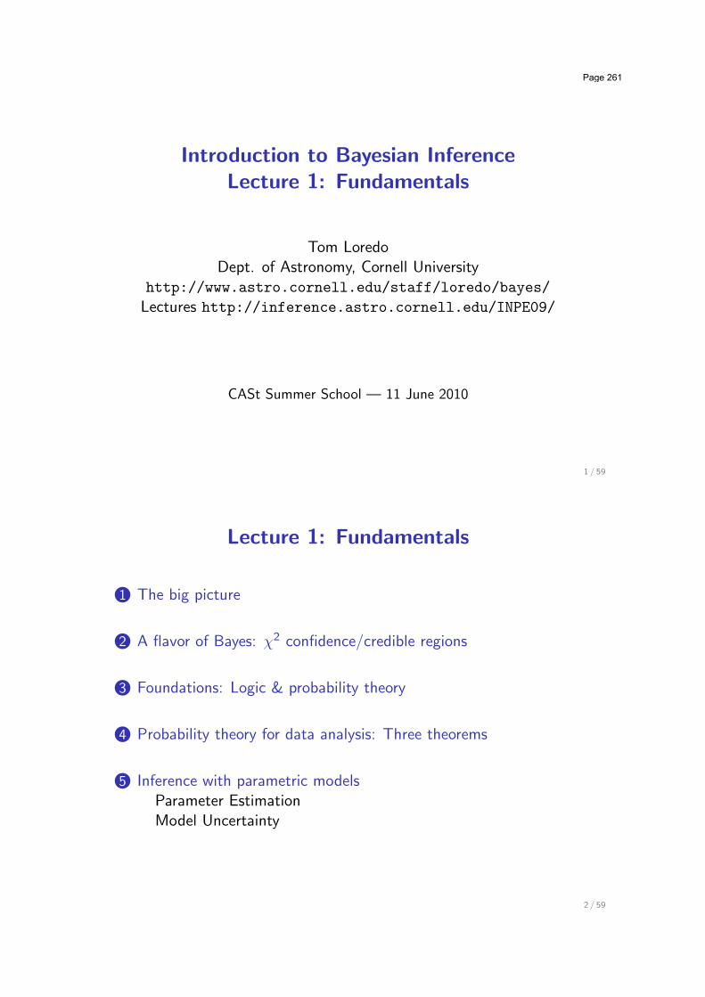
Introduction to Bayesian Inference

Lecture 1: Fundamentals

Tom LoredoDept. of Astronomy, Cornell University

http://www.astro.cornell.edu/staff/loredo/bayes/

Lectures http://inference.astro.cornell.edu/INPE09/

CASt Summer School — 11 June 2010

1 / 59

Lecture 1: Fundamentals

1 The big picture

2 A flavor of Bayes: !2 confidence/credible regions

3 Foundations: Logic & probability theory

4 Probability theory for data analysis: Three theorems

5 Inference with parametric modelsParameter EstimationModel Uncertainty

2 / 59

Page 261

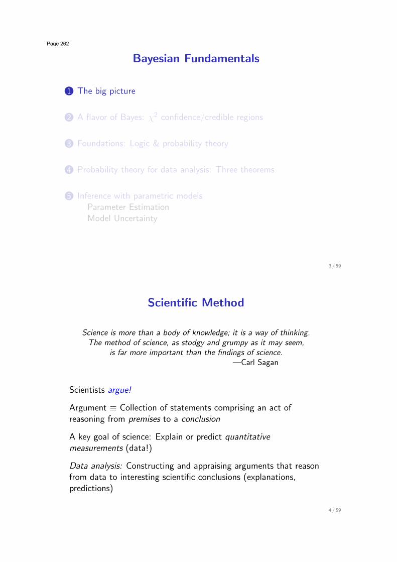
Bayesian Fundamentals

1 The big picture





3 / 59

Scientific Method

Science is more than a body of knowledge; it is a way of thinking.The method of science, as stodgy and grumpy as it may seem,

is far more important than the findings of science.—Carl Sagan

Scientists argue!

Argument ! Collection of statements comprising an act ofreasoning from premises to a conclusion

A key goal of science: Explain or predict quantitativemeasurements (data!)

Data analysis: Constructing and appraising arguments that reasonfrom data to interesting scientific conclusions (explanations,predictions)

4 / 59

62

The Role of Data

Data do not speak for themselves!

We don’t just tabulate data, we analyze data.

We gather data so they may speak for or against existinghypotheses, and guide the formation of new hypotheses.

A key role of data in science is to be among the premises inscientific arguments.

5 / 59

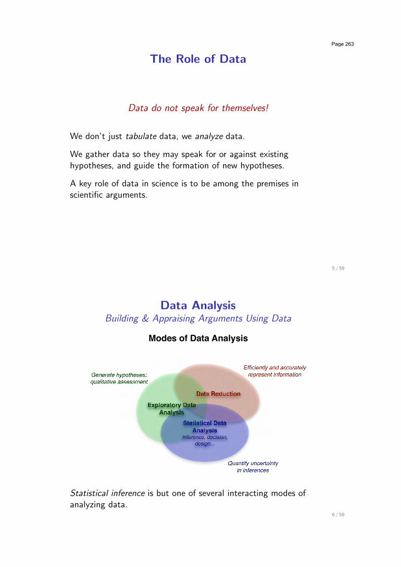
Data AnalysisBuilding & Appraising Arguments Using Data

Statistical inference is but one of several interacting modes ofanalyzing data.

6 / 59

Page 263

Bayesian Statistical Inference

• A di!erent approach to all statistical inference problems (i.e.,not just another method in the list: BLUE, maximumlikelihood, !2 testing, ANOVA, survival analysis . . . )

• Foundation: Use probability theory to quantify the strength ofarguments (i.e., a more abstract view than restricting PT todescribe variability in repeated “random” experiments)

• Focuses on deriving consequences of modeling assumptionsrather than devising and calibrating procedures

7 / 59

Frequentist vs. Bayesian Statements

“I find conclusion C based on data Dobs . . . ”

Frequentist assessment“It was found with a procedure that’s right 95% of the timeover the set {Dhyp} that includes Dobs.”Probabilities are properties of procedures, not of particularresults.

Bayesian assessment“The strength of the chain of reasoning from Dobs to C is0.95, on a scale where 1= certainty.”Probabilities are properties of specific results.Long-run performance must be separately evaluated (and istypically good by frequentist criteria).

8 / 59

Page 264


1 The big picture





9 / 59

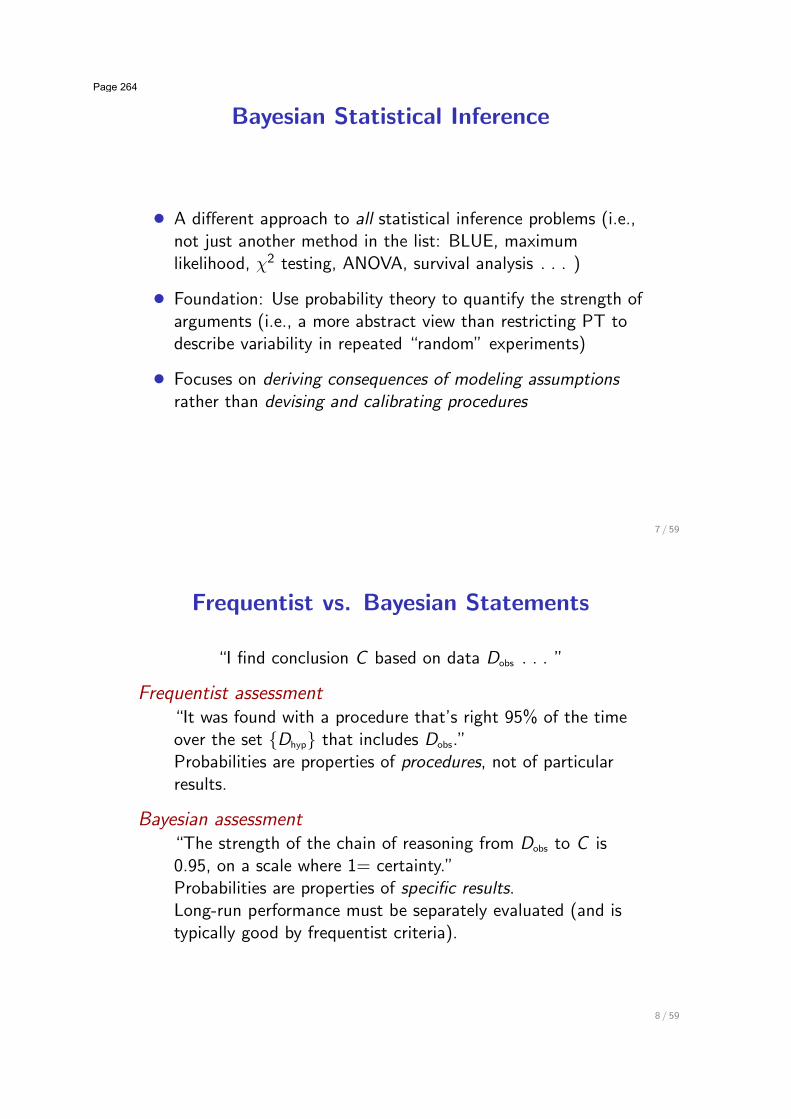
Estimating Parameters Via !2

Collect data Dobs = {di , "i}, fit with 2-parameter model via !2:

!2(A,T ) =N!

i=1

[di " fi (A,T )]2

"2i

Two classes of variables

• Data (samples) di — Known, define N-D sample space• Parameters # = (A,T ) — Unknown, define 2-D parameter space

A

T

“Best fit” # = arg min! !2(#)

Report uncertainties via !2 contours, but how do we quantifyuncertainty vs. contour level?

10 / 59

Page 265

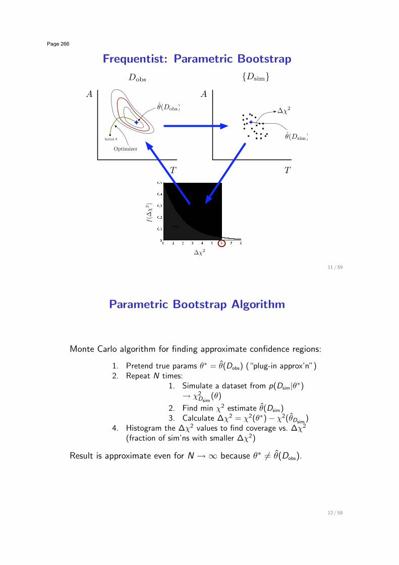
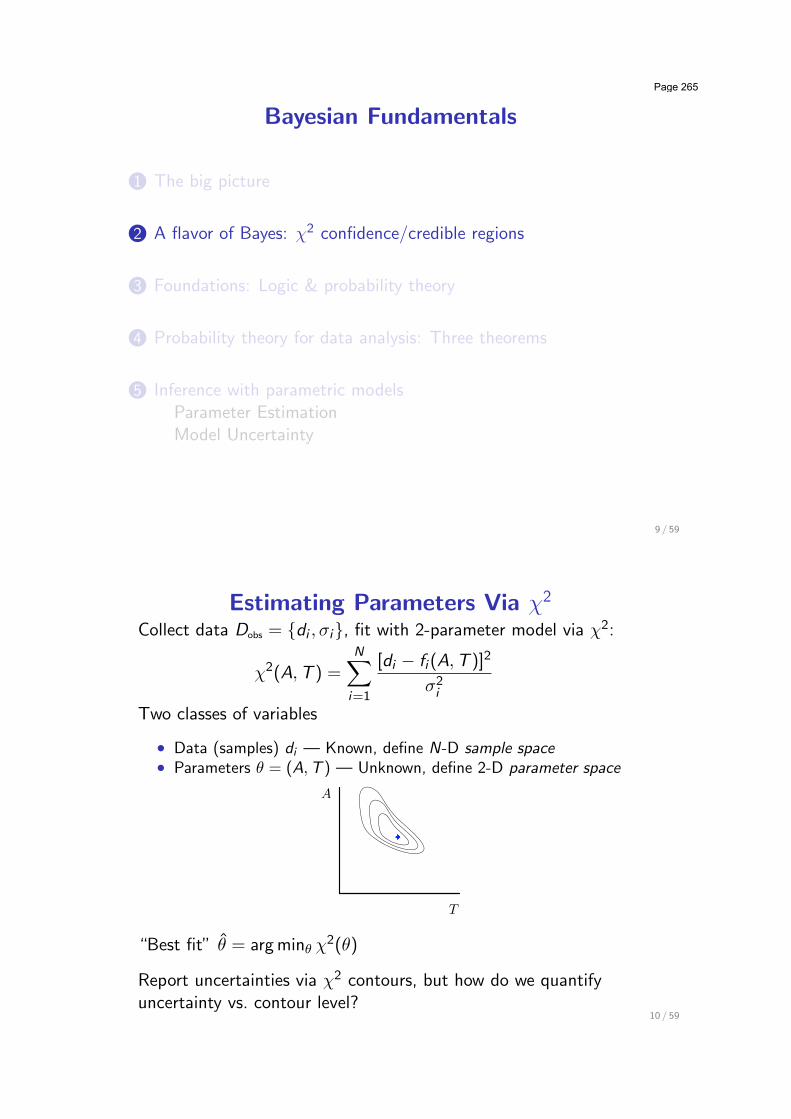
Frequentist: Parametric Bootstrap

A

T

A

T

!(Dobs)

Dobs {Dsim}

!!2

f(!

!2)

!!2

Initial !!(Dsim)

Optimizer

11 / 59

Parametric Bootstrap Algorithm

Monte Carlo algorithm for finding approximate confidence regions:

1. Pretend true params #! = #(Dobs) (“plug-in approx’n”)2. Repeat N times:

1. Simulate a dataset from p(Dsim|#!)# !2

Dsim(#)

2. Find min !2 estimate #(Dsim)3. Calculate "!2 = !2(#!) " !2(#Dsim

)4. Histogram the "!2 values to find coverage vs. "!2

(fraction of sim’ns with smaller "!2)

Result is approximate even for N # $ because #! %= #(Dobs).

12 / 59

Page 266

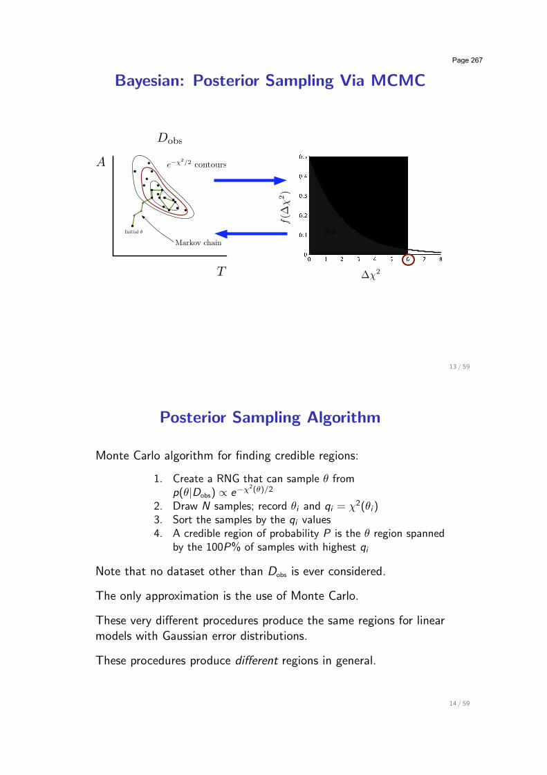
Bayesian: Posterior Sampling Via MCMC

A

T

Dobs

f(!

!2)

!!2

Initial !

e!!2/2

contours

Markov chain

13 / 59

Posterior Sampling Algorithm

Monte Carlo algorithm for finding credible regions:

1. Create a RNG that can sample # fromp(#|Dobs) & e"!

2(")/2

2. Draw N samples; record #i and qi = !2(#i )3. Sort the samples by the qi values4. A credible region of probability P is the # region spanned

by the 100P% of samples with highest qi

Note that no dataset other than Dobs is ever considered.

The only approximation is the use of Monte Carlo.

These very di!erent procedures produce the same regions for linearmodels with Gaussian error distributions.

These procedures produce di!erent regions in general.

14 / 59

Page 267


1 The big picture





15 / 59

Logic—Some Essentials“Logic can be defined as the analysis and appraisal of arguments”

—Gensler, Intro to Logic

Build arguments with propositions and logicaloperators/connectives:

• Propositions: Statements that may be true or false

P : Universe can be modeled with #CDM

A : $tot ' [0.9, 1.1]

B : $! is not 0

B : “not B,” i.e.,$! = 0

• Connectives:

A ( B : A andB are both true

A ) B : A orB is true, or both are

16 / 59

Page 268

Arguments

Argument: Assertion that an hypothesized conclusion, H, followsfrom premises, P = {A,B, C , . . .} (take “,” = “and”)

Notation:

H|P : Premises P imply H

H may be deduced from PH follows from PH is true given that P is true

Arguments are (compound) propositions.

Central role of arguments # special terminology for true/false:

• A true argument is valid

• A false argument is invalid or fallacious

17 / 59

Valid vs. Sound Arguments

Content vs. form

• An argument is factually correct i! all of its premises are true(it has “good content”).

• An argument is valid i! its conclusion follows from itspremises (it has “good form”).

• An argument is sound i! it is both factually correct and valid(it has good form and content).

Deductive logic and probability theory address validity.

We want to make sound arguments. There is no formal approachfor addressing factual correctness # there is always a subjectiveelement to an argument.

18 / 59

Page 269

Factual Correctness

Passing the buckAlthough logic can teach us something about validity andinvalidity, it can teach us very little about factual correctness.The question of the truth or falsity of individual statements isprimarily the subject matter of the sciences.

— Hardegree, Symbolic Logic

An open issueTo test the truth or falsehood of premisses is the task ofscience. . . . But as a matter of fact we are interested in, andmust often depend upon, the correctness of arguments whosepremisses are not known to be true.

— Copi, Introduction to Logic

19 / 59

Premises

• Facts — Things known to be true, e.g. observed data

• “Obvious” assumptions — Axioms, postulates, e.g., Euclid’sfirst 4 postulates (line segment b/t 2 points; congruency ofright angles . . . )

• “Reasonable” or “working” assumptions — E.g., Euclid’s fifthpostulate (parallel lines)

• Desperate presumption!

• Conclusions from other arguments

Premises define a fixed context in which arguments may beassessed.

Premises are considered “given”—if only for the sake of theargument!

20 / 59

Page 270

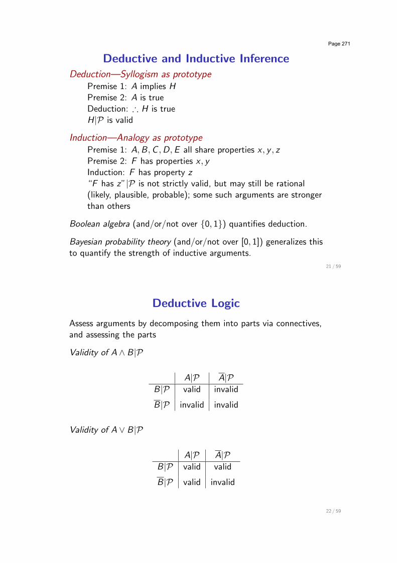
Deductive and Inductive Inference

Deduction—Syllogism as prototypePremise 1: A implies HPremise 2: A is trueDeduction: ! H is trueH|P is valid

Induction—Analogy as prototypePremise 1: A,B, C , D, E all share properties x , y , zPremise 2: F has properties x , yInduction: F has property z“F has z”|P is not strictly valid, but may still be rational(likely, plausible, probable); some such arguments are strongerthan others

Boolean algebra (and/or/not over {0, 1}) quantifies deduction.

Bayesian probability theory (and/or/not over [0, 1]) generalizes thisto quantify the strength of inductive arguments.

21 / 59

Deductive Logic

Assess arguments by decomposing them into parts via connectives,and assessing the parts

Validity of A ( B|P

A|P A|PB|P valid invalid

B|P invalid invalid

Validity of A ) B|P

A|P A|PB|P valid valid

B|P valid invalid

22 / 59

Page 271

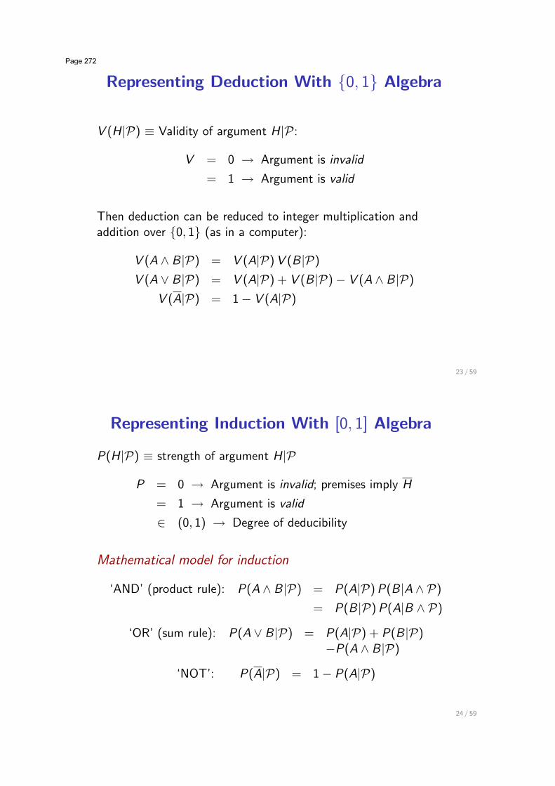
Representing Deduction With {0, 1} Algebra

V (H|P) ! Validity of argument H|P:

V = 0 # Argument is invalid

= 1 # Argument is valid

Then deduction can be reduced to integer multiplication andaddition over {0, 1} (as in a computer):

V (A ( B|P) = V (A|P)V (B|P)

V (A ) B|P) = V (A|P) + V (B|P) " V (A ( B|P)

V (A|P) = 1 " V (A|P)

23 / 59

Representing Induction With [0, 1] Algebra

P(H|P) ! strength of argument H|P

P = 0 # Argument is invalid; premises imply H

= 1 # Argument is valid

' (0, 1) # Degree of deducibility

Mathematical model for induction

‘AND’ (product rule): P(A ( B|P) = P(A|P)P(B|A ( P)

= P(B|P)P(A|B ( P)

‘OR’ (sum rule): P(A ) B|P) = P(A|P) + P(B|P)"P(A ( B|P)

‘NOT’: P(A|P) = 1 " P(A|P)

24 / 59

Page 272

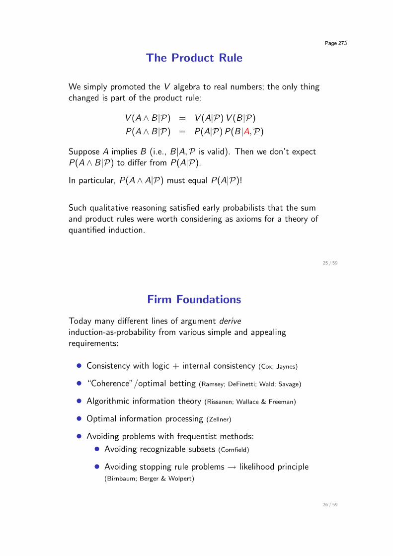
The Product Rule

We simply promoted the V algebra to real numbers; the only thingchanged is part of the product rule:

V (A ( B|P) = V (A|P)V (B|P)

P(A ( B|P) = P(A|P)P(B|A,P)

Suppose A implies B (i.e., B|A,P is valid). Then we don’t expectP(A ( B|P) to di!er from P(A|P).

In particular, P(A ( A|P) must equal P(A|P)!

Such qualitative reasoning satisfied early probabilists that the sumand product rules were worth considering as axioms for a theory ofquantified induction.

25 / 59

Firm Foundations

Today many di!erent lines of argument deriveinduction-as-probability from various simple and appealingrequirements:

• Consistency with logic + internal consistency (Cox; Jaynes)

• “Coherence”/optimal betting (Ramsey; DeFinetti; Wald; Savage)

• Algorithmic information theory (Rissanen; Wallace & Freeman)

• Optimal information processing (Zellner)

• Avoiding problems with frequentist methods:

• Avoiding recognizable subsets (Cornfield)

• Avoiding stopping rule problems # likelihood principle(Birnbaum; Berger & Wolpert)

26 / 59

Page 273

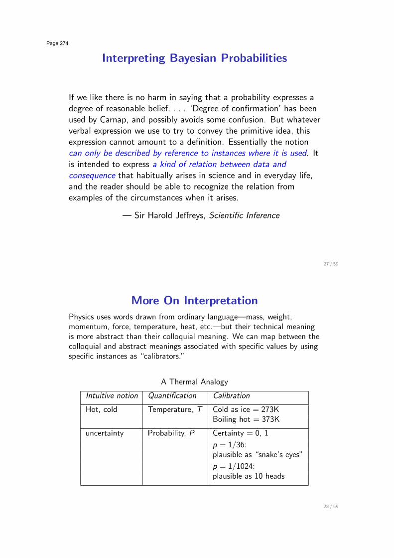
Interpreting Bayesian Probabilities

If we like there is no harm in saying that a probability expresses adegree of reasonable belief. . . . ‘Degree of confirmation’ has beenused by Carnap, and possibly avoids some confusion. But whateververbal expression we use to try to convey the primitive idea, thisexpression cannot amount to a definition. Essentially the notioncan only be described by reference to instances where it is used. Itis intended to express a kind of relation between data andconsequence that habitually arises in science and in everyday life,and the reader should be able to recognize the relation fromexamples of the circumstances when it arises.

— Sir Harold Je!reys, Scientific Inference

27 / 59

More On Interpretation

Physics uses words drawn from ordinary language—mass, weight,momentum, force, temperature, heat, etc.—but their technical meaningis more abstract than their colloquial meaning. We can map between thecolloquial and abstract meanings associated with specific values by usingspecific instances as “calibrators.”

A Thermal Analogy

Intuitive notion Quantification Calibration

Hot, cold Temperature, T Cold as ice = 273KBoiling hot = 373K

uncertainty Probability, P Certainty = 0, 1

p = 1/36:plausible as “snake’s eyes”

p = 1/1024:plausible as 10 heads

28 / 59

Page 274

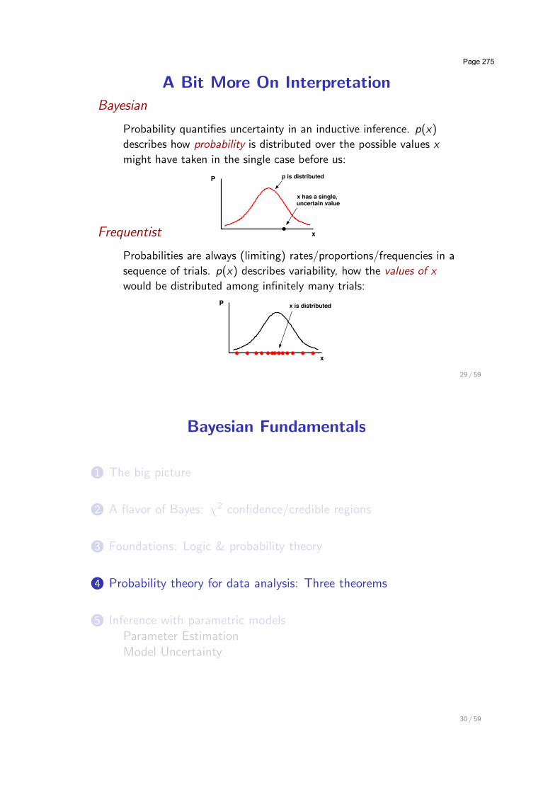
A Bit More On Interpretation

Bayesian

Probability quantifies uncertainty in an inductive inference. p(x)describes how probability is distributed over the possible values xmight have taken in the single case before us:

P

x

p is distributed

x has a single,uncertain value

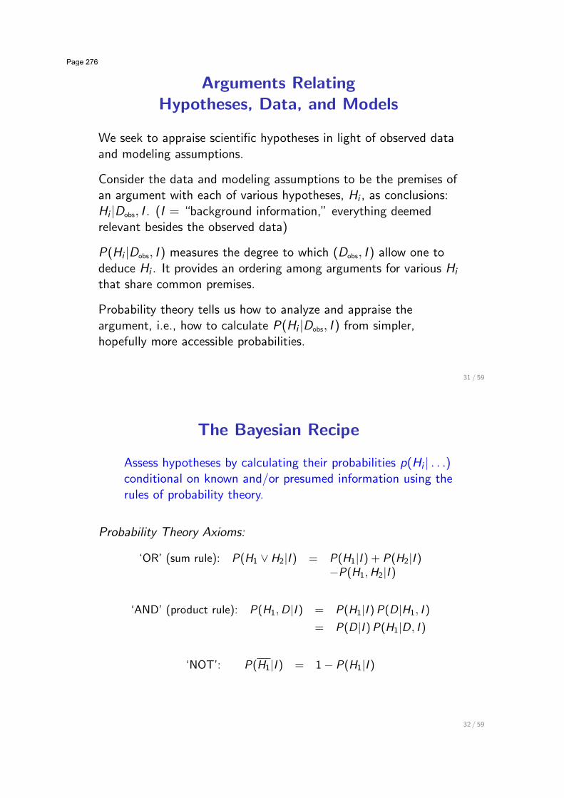
Frequentist

Probabilities are always (limiting) rates/proportions/frequencies in asequence of trials. p(x) describes variability, how the values of xwould be distributed among infinitely many trials:

x is distributed

x

P

29 / 59


1 The big picture





30 / 59

Page 275

Arguments Relating

Hypotheses, Data, and Models

We seek to appraise scientific hypotheses in light of observed dataand modeling assumptions.

Consider the data and modeling assumptions to be the premises ofan argument with each of various hypotheses, Hi , as conclusions:Hi |Dobs, I . (I = “background information,” everything deemedrelevant besides the observed data)

P(Hi |Dobs, I ) measures the degree to which (Dobs, I ) allow one todeduce Hi . It provides an ordering among arguments for various Hi

that share common premises.

Probability theory tells us how to analyze and appraise theargument, i.e., how to calculate P(Hi |Dobs, I ) from simpler,hopefully more accessible probabilities.

31 / 59

The Bayesian Recipe

Assess hypotheses by calculating their probabilities p(Hi | . . .)conditional on known and/or presumed information using therules of probability theory.

Probability Theory Axioms:

‘OR’ (sum rule): P(H1 ) H2|I ) = P(H1|I ) + P(H2|I )"P(H1,H2|I )

‘AND’ (product rule): P(H1,D|I ) = P(H1|I )P(D|H1, I )

= P(D|I )P(H1|D, I )

‘NOT’: P(H1|I ) = 1 " P(H1|I )

32 / 59

Page 276

Three Important Theorems

Bayes’s Theorem (BT)Consider P(Hi , Dobs|I ) using the product rule:

P(Hi , Dobs|I ) = P(Hi |I )P(Dobs|Hi , I )

= P(Dobs|I )P(Hi |Dobs, I )

Solve for the posterior probability:

P(Hi |Dobs, I ) = P(Hi |I )P(Dobs|Hi , I )

P(Dobs|I )

Theorem holds for any propositions, but for hypotheses &data the factors have names:

posterior & prior * likelihood

norm. const. P(Dobs|I ) = prior predictive

33 / 59

Law of Total Probability (LTP)Consider exclusive, exhaustive {Bi} (I asserts one of themmust be true),

!

i

P(A,Bi |I ) =!

i

P(Bi |A, I )P(A|I ) = P(A|I )

=!

i

P(Bi |I )P(A|Bi , I )

If we do not see how to get P(A|I ) directly, we can find a set{Bi} and use it as a “basis”—extend the conversation:

P(A|I ) =!

i

P(Bi |I )P(A|Bi , I )

If our problem already has Bi in it, we can use LTP to getP(A|I ) from the joint probabilities—marginalization:

P(A|I ) =!

i

P(A,Bi |I )

34 / 59

Page 277

Example: Take A = Dobs, Bi = Hi ; then

P(Dobs|I ) =!

i

P(Dobs,Hi |I )

=!

i

P(Hi |I )P(Dobs|Hi , I )

prior predictive for Dobs = Average likelihood for Hi

(a.k.a. marginal likelihood)

NormalizationFor exclusive, exhaustive Hi ,

!

i

P(Hi | · · · ) = 1

35 / 59

Well-Posed ProblemsThe rules express desired probabilities in terms of otherprobabilities.

To get a numerical value out, at some point we have to putnumerical values in.

Direct probabilities are probabilities with numerical valuesdetermined directly by premises (via modeling assumptions,symmetry arguments, previous calculations, desperatepresumption . . . ).

An inference problem is well posed only if all the neededprobabilities are assignable based on the premises. We may need toadd new assumptions as we see what needs to be assigned. Wemay not be entirely comfortable with what we need to assume!(Remember Euclid’s fifth postulate!)

Should explore how results depend on uncomfortable assumptions(“robustness”).

36 / 59

Page 278

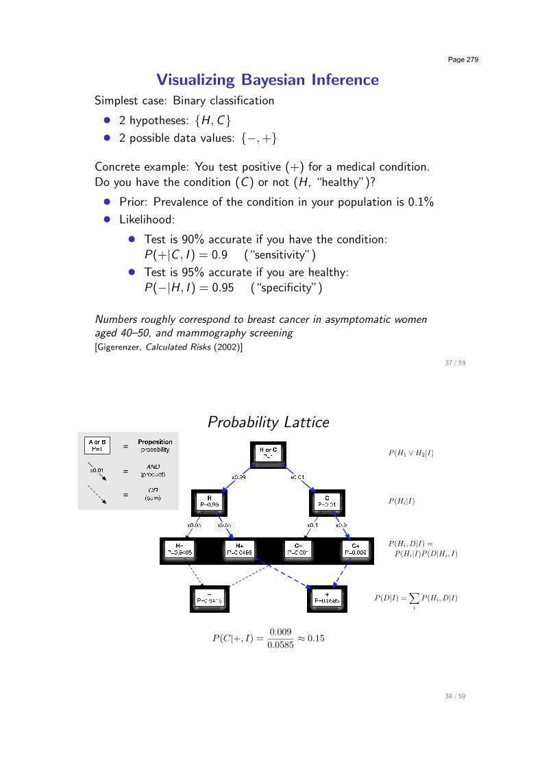
Visualizing Bayesian InferenceSimplest case: Binary classification

• 2 hypotheses: {H, C}• 2 possible data values: {", +}

Concrete example: You test positive (+) for a medical condition.Do you have the condition (C ) or not (H, “healthy”)?

• Prior: Prevalence of the condition in your population is 0.1%

• Likelihood:

• Test is 90% accurate if you have the condition:P(+|C , I ) = 0.9 (“sensitivity”)

• Test is 95% accurate if you are healthy:P("|H, I ) = 0.95 (“specificity”)

Numbers roughly correspond to breast cancer in asymptomatic womenaged 40–50, and mammography screening[Gigerenzer, Calculated Risks (2002)]

37 / 59

Probability Lattice

P (Hi|I)

P (Hi, D|I) =P (Hi|I)P (D|Hi, I)

P (D|I) =!

i

P (Hi, D|I)

P (C|+, I) =0.009

0.0585! 0.15

P (H1 ! H2|I)

38 / 59

Page 279

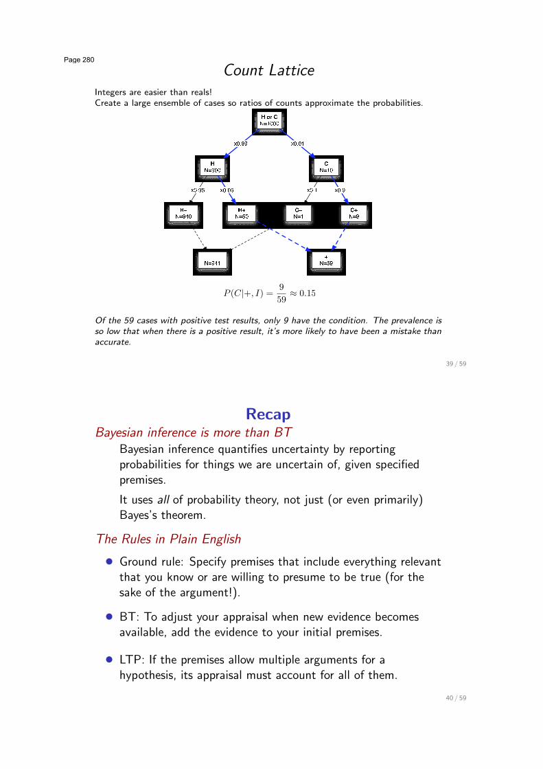
Count LatticeIntegers are easier than reals!Create a large ensemble of cases so ratios of counts approximate the probabilities.

P (C|+, I) =9

59! 0.15

Of the 59 cases with positive test results, only 9 have the condition. The prevalence isso low that when there is a positive result, it’s more likely to have been a mistake thanaccurate.

39 / 59

RecapBayesian inference is more than BT

Bayesian inference quantifies uncertainty by reportingprobabilities for things we are uncertain of, given specifiedpremises.

It uses all of probability theory, not just (or even primarily)Bayes’s theorem.

The Rules in Plain English

• Ground rule: Specify premises that include everything relevantthat you know or are willing to presume to be true (for thesake of the argument!).

• BT: To adjust your appraisal when new evidence becomesavailable, add the evidence to your initial premises.

• LTP: If the premises allow multiple arguments for ahypothesis, its appraisal must account for all of them.

40 / 59

Page 280


1 The big picture





41 / 59

Inference With Parametric Models

Models Mi (i = 1 to N), each with parameters #i , each imply asampling dist’n (conditional predictive dist’n for possible data):

p(D|#i , Mi )

The #i dependence when we fix attention on the observed data isthe likelihood function:

Li (#i ) ! p(Dobs|#i , Mi )

We may be uncertain about i (model uncertainty) or #i (parameteruncertainty).

Henceforth we will only consider the actually observed data, so we dropthe cumbersome subscript: D = Dobs.

42 / 59

Page 281

Three Classes of Problems

Parameter EstimationPremise = choice of model (pick specific i)# What can we say about #i?

Model Assessment

• Model comparison: Premise = {Mi}# What can we say about i?

• Model adequacy/GoF: Premise = M1) “all” alternatives# Is M1 adequate?

Model AveragingModels share some common params: #i = {$, %i}# What can we say about $ w/o committing to one model?(Examples: systematic error, prediction)

43 / 59

Parameter Estimation

Problem statementI = Model M with parameters # (+ any add’l info)

Hi = statements about #; e.g. “# ' [2.5, 3.5],” or “# > 0”

Probability for any such statement can be found using aprobability density function (PDF) for #:

P(# ' [#, # + d#]| · · · ) = f (#)d#

= p(#| · · · )d#

Posterior probability density

p(#|D, M) =p(#|M) L(#)"d# p(#|M) L(#)

44 / 59

Page 282

Summaries of posterior

• “Best fit” values:• Mode, #, maximizes p(#|D,M)• Posterior mean, +#, =

"d# # p(#|D,M)

• Uncertainties:• Credible region " of probability C :

C = P(# ' "|D,M) ="" d# p(#|D,M)

Highest Posterior Density (HPD) region has p(#|D,M) higherinside than outside

• Posterior standard deviation, variance, covariances

• Marginal distributions• Interesting parameters $, nuisance parameters %• Marginal dist’n for $: p($|D,M) =

"d% p($, %|D,M)

45 / 59

Nuisance Parameters and Marginalization

To model most data, we need to introduce parameters besidesthose of ultimate interest: nuisance parameters.

ExampleWe have data from measuring a rate r = s + b that is a sumof an interesting signal s and a background b.

We have additional data just about b.

What do the data tell us about s?

46 / 59

Page 283

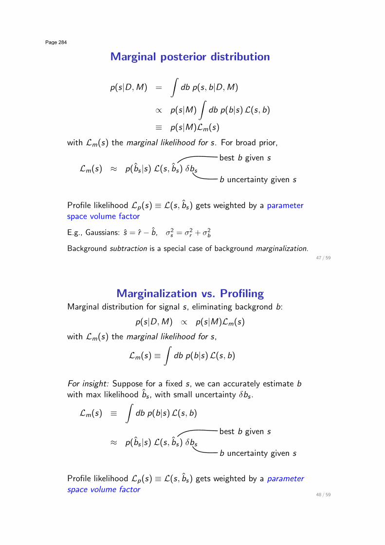
Marginal posterior distribution

p(s|D, M) =

#db p(s, b|D, M)

& p(s|M)

#db p(b|s)L(s, b)

! p(s|M)Lm(s)

with Lm(s) the marginal likelihood for s. For broad prior,

Lm(s) - p(bs |s) L(s, bs) &bs

best b given s

b uncertainty given s

Profile likelihood Lp(s) ! L(s, bs) gets weighted by a parameterspace volume factor

E.g., Gaussians: s = r " b, "2s = "2

r + "2b

Background subtraction is a special case of background marginalization.47 / 59

Marginalization vs. ProfilingMarginal distribution for signal s, eliminating backgrond b:

p(s|D, M) & p(s|M)Lm(s)

with Lm(s) the marginal likelihood for s,

Lm(s) !#

db p(b|s)L(s, b)

For insight: Suppose for a fixed s, we can accurately estimate bwith max likelihood bs , with small uncertainty &bs .

Lm(s) !#

db p(b|s)L(s, b)

- p(bs |s) L(s, bs) &bs

best b given s

b uncertainty given s

Profile likelihood Lp(s) ! L(s, bs) gets weighted by a parameterspace volume factor

48 / 59

Page 284

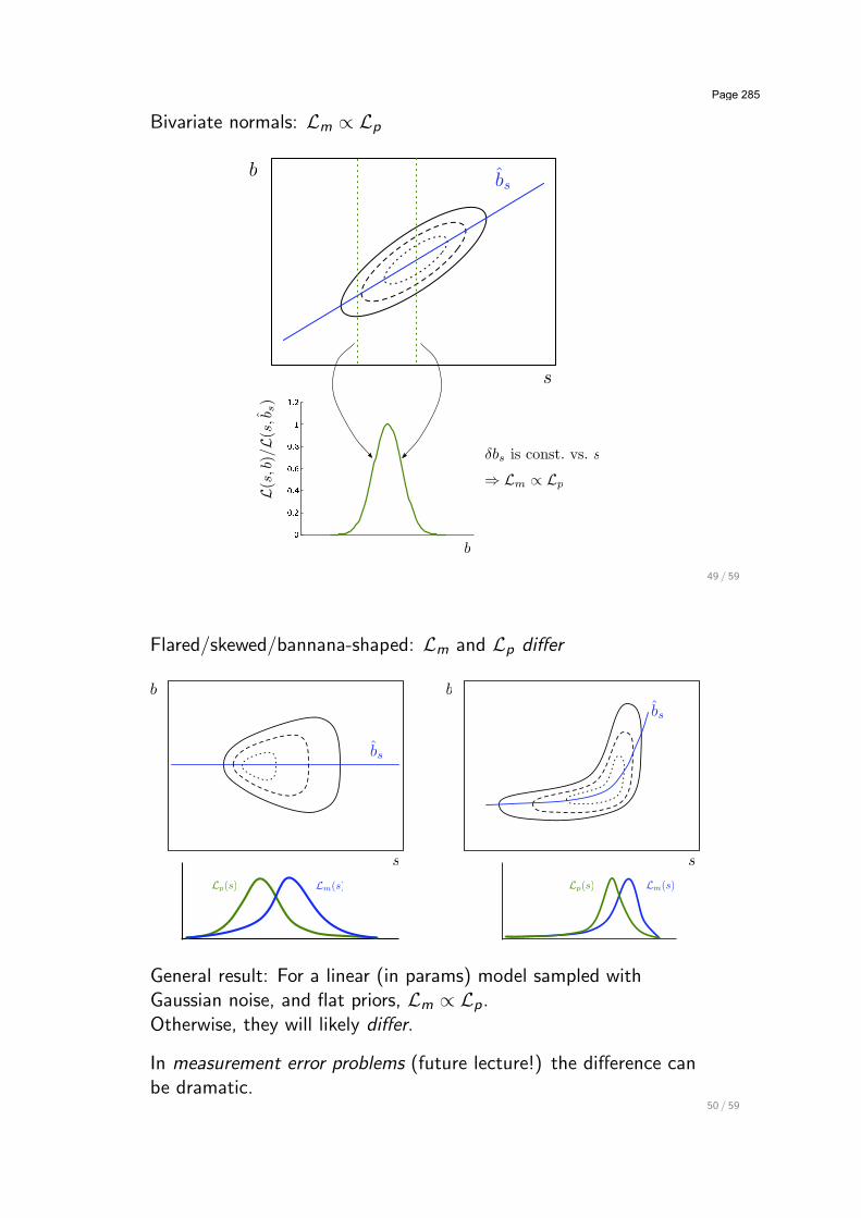
Bivariate normals: Lm & Lp

s

bbs

b

L(s

,b)/L

(s,b

s)

!bs is const. vs. s

! Lm " Lp

49 / 59

Flared/skewed/bannana-shaped: Lm and Lp di!er

Lp(s) Lm(s)

s

b

bs

s

b

bs

Lp(s) Lm(s)

General result: For a linear (in params) model sampled withGaussian noise, and flat priors, Lm & Lp.Otherwise, they will likely di!er.

In measurement error problems (future lecture!) the di!erence canbe dramatic.

50 / 59

Page 285

Many Roles for MarginalizationEliminate nuisance parameters

p($|D,M) =

#d% p($, %|D,M)

Propagate uncertainty

Model has parameters #; what can we infer about F = f (#)?

p(F |D,M) =

#d# p(F , #|D,M) =

#d# p(#|D,M) p(F |#,M)

=

#d# p(#|D,M) &[F " f (#)] [single-valued case]

Prediction

Given a model with parameters # and present data D, predict futuredata D # (e.g., for experimental design):

p(D #|D,M) =

#d# p(D #, #|D,M) =

#d# p(#|D,M) p(D #|#,M)

Model comparison. . .51 / 59

Model ComparisonProblem statement

I = (M1 ) M2 ) . . .) — Specify a set of models.Hi = Mi — Hypothesis chooses a model.

Posterior probability for a model

p(Mi |D, I ) = p(Mi |I )p(D|Mi , I )

p(D|I )& p(Mi |I )L(Mi )

But L(Mi ) = p(D|Mi ) ="

d#i p(#i |Mi )p(D|#i , Mi ).

Likelihood for model = Average likelihood for its parameters

L(Mi ) = +L(#i ),

Varied terminology: Prior predictive = Average likelihood = Globallikelihood = Marginal likelihood = (Weight of) Evidence for model

52 / 59

Page 286

Odds and Bayes factors

A ratio of probabilities for two propositions using the samepremises is called the odds favoring one over the other:

Oij !p(Mi |D, I )

p(Mj |D, I )

=p(Mi |I )p(Mj |I )

*p(D|Mi , I )

p(D|Mj , I )

The data-dependent part is called the Bayes factor:

Bij !p(D|Mi , I )

p(D|Mj , I )

It is a likelihood ratio; the BF terminology is usually reserved forcases when the likelihoods are marginal/average likelihoods.

53 / 59

An Automatic Occam’s Razor

Predictive probabilities can favor simpler models

p(D|Mi ) =

#d#i p(#i |M) L(#i )

DobsD

P(D|H)

Complicated H

Simple H

54 / 59

Page 287

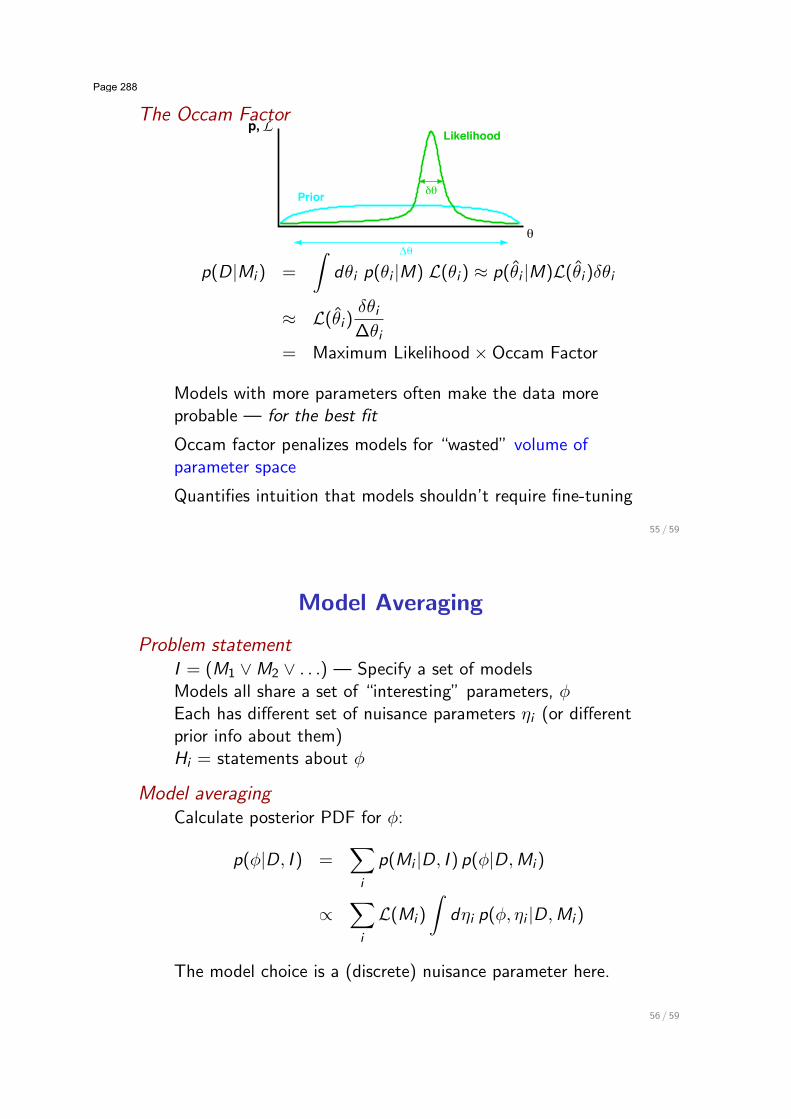
The Occam Factorp,L

θΔθ

δθPrior

Likelihood

p(D|Mi ) =

#d#i p(#i |M) L(#i ) - p(#i |M)L(#i )&#i

- L(#i )&#i

"#i

= Maximum Likelihood * Occam Factor

Models with more parameters often make the data moreprobable — for the best fit

Occam factor penalizes models for “wasted” volume ofparameter space

Quantifies intuition that models shouldn’t require fine-tuning

55 / 59

Model Averaging

Problem statementI = (M1 ) M2 ) . . .) — Specify a set of modelsModels all share a set of “interesting” parameters, $

Each has di!erent set of nuisance parameters %i (or di!erentprior info about them)Hi = statements about $

Model averagingCalculate posterior PDF for $:

p($|D, I ) =!

i

p(Mi |D, I ) p($|D, Mi )

&!

i

L(Mi )

#d%i p($, %i |D, Mi )

The model choice is a (discrete) nuisance parameter here.

56 / 59

8

Theme: Parameter Space Volume

Bayesian calculations sum/integrate over parameter/hypothesisspace!

(Frequentist calculations average over sample space & typically optimize

over parameter space.)

• Marginalization weights the profile likelihood by a volumefactor for the nuisance parameters.

• Model likelihoods have Occam factors resulting fromparameter space volume factors.

Many virtues of Bayesian methods can be attributed to thisaccounting for the “size” of parameter space. This idea does notarise naturally in frequentist statistics (but it can be added “byhand”).

57 / 59

Roles of the Prior

Prior has two roles

• Incorporate any relevant prior information

• Convert likelihood from “intensity” to “measure”

# Accounts for size of hypothesis space

Physical analogy

Heat: Q =

#dV cv (r)T (r)

Probability: P &#

d# p(#|I )L(#)

Maximum likelihood focuses on the “hottest” hypotheses.Bayes focuses on the hypotheses with the most “heat.”A high-T region may contain little heat if its cv is low or ifits volume is small.A high-L region may contain little probability if its prior is low or ifits volume is small.

58 / 59

Page 289

Recap of Key Ideas

• Probability as generalized logic for appraising arguments

• Three theorems: BT, LTP, Normalization

• Calculations characterized by parameter space integrals• Credible regions, posterior expectations• Marginalization over nuisance parameters• Occam’s razor via marginal likelihoods• Do not integrate/average over hypothetical data

59 / 59

Page 290

Intro duction to Ba yesian Inference Lecture 1: F undamentals · Ba yesian F undamentals 1 The big...

Documents

Transcript of Intro duction to Ba yesian Inference Lecture 1: F undamentals · Ba yesian F undamentals 1 The big...