Interaction between Atoms and Light - Department of...
171
Interaction between Atoms and Light Dr. Karl-Peter Marzlin 2003
-
Upload
nguyenhanh -
Category
Documents
-
view
223 -
download
4
Transcript of Interaction between Atoms and Light - Department of...
Interaction between Atoms and Light
Dr. Karl-Peter Marzlin
2003

2
Contents
1 Maxwell’s Equations and Gauge Fields 11.1 Maxwell’s Equations . . . . . . . . . . . . . . . . . . . . . . . . . . . . . . . .11.2 Scalar Potential and Vector Potential . . . . . . . . . . . . . . . . . . . . . . . .31.3 Gauge transformations . . . . . . . . . . . . . . . . . . . . . . . . . . . . . . .41.4 Multipole Expansion . . . . . . . . . . . . . . . . . . . . . . . . . . . . . . . .61.5 Electrodynamics in Dielectric Media . . . . . . . . . . . . . . . . . . . . . . . .101.6 Macroscopic Maxwell equations . . . . . . . . . . . . . . . . . . . . . . . . . .111.7 Plane Waves . . . . . . . . . . . . . . . . . . . . . . . . . . . . . . . . . . . . .14
2 Quantum Field Theory of Light - QED 172.1 Many-Particle Theory of Quantum Mechanics . . . . . . . . . . . . . . . . . . .17
2.1.1 Fock Space and Number Representation . . . . . . . . . . . . . . . . . .182.1.2 Creation and Anihilation Operators . . . . . . . . . . . . . . . . . . . .202.1.3 The Field Operator . . . . . . . . . . . . . . . . . . . . . . . . . . . . .212.1.4 Second Quantization . . . . . . . . . . . . . . . . . . . . . . . . . . . .242.1.5 Summary of the construction of a many-particle theory . . . . . . . . . .252.1.6 Quantization in Coulomb Gauge . . . . . . . . . . . . . . . . . . . . . .25
2.2 Coherent States . . . . . . . . . . . . . . . . . . . . . . . . . . . . . . . . . . .302.3 Classical and Quantum Mechanical Interference . . . . . . . . . . . . . . . . . .352.4 Remarks on the Quantization Procedure for other Gauges . . . . . . . . . . . . .37
3 Quantum Mechanics of Atoms: a short Review 393.1 The Hydrogen Atom, Parity . . . . . . . . . . . . . . . . . . . . . . . . . . . .393.2 Fine structure and spin . . . . . . . . . . . . . . . . . . . . . . . . . . . . . . .403.3 Hyperfine structure . . . . . . . . . . . . . . . . . . . . . . . . . . . . . . . . .41
4 The Interaction between Atoms and Light 434.1 Minimal Coupling . . . . . . . . . . . . . . . . . . . . . . . . . . . . . . . . . .43
4.1.1 Derivation of Minimal Coupling . . . . . . . . . . . . . . . . . . . . . .434.1.2 Gauge Invariance of Minimal Coupling . . . . . . . . . . . . . . . . . .45
4.2 The Power-Zienau-Woolley Transformation . . . . . . . . . . . . . . . . . . . .464.2.1 The Basic Idea . . . . . . . . . . . . . . . . . . . . . . . . . . . . . . .464.2.2 The Complete Transformation . . . . . . . . . . . . . . . . . . . . . . .47
4 CONTENTS
4.3 Dipole approximation and dipole coupling . . . . . . . . . . . . . . . . . . . . .554.4 Selection rules for atoms . . . . . . . . . . . . . . . . . . . . . . . . . . . . . .56
5 The two-level model for atoms 615.1 Derivation of two-level systems . . . . . . . . . . . . . . . . . . . . . . . . . .62
5.1.1 Representation of operators . . . . . . . . . . . . . . . . . . . . . . . .635.1.2 Coupling between a two-level atom and the electromagnetic field . . . .64
5.2 Rabi oscillations and Landau-Zener transitions . . . . . . . . . . . . . . . . . .675.2.1 Landau-Zener transitions . . . . . . . . . . . . . . . . . . . . . . . . . .71
5.3 Dressed States . . . . . . . . . . . . . . . . . . . . . . . . . . . . . . . . . . .735.3.1 Dressed states in a cavity . . . . . . . . . . . . . . . . . . . . . . . . . .74
5.4 Models with few levels, dark states, Raman transitions . . . . . . . . . . . . . .775.4.1 Dark States . . . . . . . . . . . . . . . . . . . . . . . . . . . . . . . . .775.4.2 Raman transitions . . . . . . . . . . . . . . . . . . . . . . . . . . . . .81
5.5 Adiabatc theorem, STIRAP . . . . . . . . . . . . . . . . . . . . . . . . . . . . .835.5.1 Application of the adiabatic theorem to dark states . . . . . . . . . . . .85
6 Atomoptik 876.1 Grundlegendes Prinzip . . . . . . . . . . . . . . . . . . . . . . . . . . . . . . .876.2 Atom”=Interferometrie . . . . . . . . . . . . . . . . . . . . . . . . . . . . . . .89
6.2.1 Ramsey-Borde”=Interferometer (Borde 1988, Riehle 1991) . . . . . . . .896.2.2 Atomic fountain (Kasevich & Chu 1991) . . . . . . . . . . . . . . . . .91
6.3 Optische Potentiale . . . . . . . . . . . . . . . . . . . . . . . . . . . . . . . . .926.3.1 Laufender Laser mit Gau”s”=Profil . . . . . . . . . . . . . . . . . . . .936.3.2 Stehender Doughnut-Laser . . . . . . . . . . . . . . . . . . . . . . . . .936.3.3 Evaneszente Lichtfelder . . . . . . . . . . . . . . . . . . . . . . . . . .946.3.4 Linsen f”ur einen Atomstrahl . . . . . . . . . . . . . . . . . . . . . . . .94
7 Incoherent Interaction and Density Matrix 977.1 Density Matrix Formalism . . . . . . . . . . . . . . . . . . . . . . . . . . . . .977.2 Liouville Equation, Superoperators . . . . . . . . . . . . . . . . . . . . . . . . .1007.3 Reduced density matrix, Zwanzig’s Master Equation . . . . . . . . . . . . . . .103
7.3.1 Reduced Density Matrix, Projection Superoperators . . . . . . . . . . . .1037.3.2 Zwanzig’s Master Equation . . . . . . . . . . . . . . . . . . . . . . . .105
7.4 Spontaneous Emission . . . . . . . . . . . . . . . . . . . . . . . . . . . . . . .1127.5 Spontaneous emission cancellation through interference . . . . . . . . . . . . . .118
8 Laser”=K uhlen von Atomen 1218.1 Allgemeines zur Kuhlung von Atomen . . . . . . . . . . . . . . . . . . . . . . .1218.2 Doppler”=Kuhlung . . . . . . . . . . . . . . . . . . . . . . . . . . . . . . . . .121
8.2.1 Das Prinzip . . . . . . . . . . . . . . . . . . . . . . . . . . . . . . . . .1228.2.2 Theoretische Beschreibung . . . . . . . . . . . . . . . . . . . . . . . . .122
8.3 VSCPT . . . . . . . . . . . . . . . . . . . . . . . . . . . . . . . . . . . . . . .125
CONTENTS 5
9 Electromagnetically induced transparency 1279.1 The Maxwell-Bloch equations . . . . . . . . . . . . . . . . . . . . . . . . . . .1279.2 Index of refraction for a two-level atom . . . . . . . . . . . . . . . . . . . . . .1289.3 Electromagnetically induced transparency and dark states . . . . . . . . . . . . .131
10 Photonic band gaps 135
11 Bose-Einstein-Kondensate 14111.1 Vielteilchentheorie bosonischer Atome . . . . . . . . . . . . . . . . . . . . . . .14111.2 Der Bose”=Einstein”=Phasenubergang . . . . . . . . . . . . . . . . . . . . . . .14311.3 Atome mit Wechselwirkung, kollektive Wellenfunktion . . . . . . . . . . . . . .14511.4 Einfache Anwendungen der Gross”=Pitaevskii”=Gleichung . . . . . . . . . . . .148
11.4.1 BECs in harmonischen Fallen , Thomas”=Fermi”=Naherung . . . . . . .14811.4.2 Solitonen . . . . . . . . . . . . . . . . . . . . . . . . . . . . . . . . . .149
12 Appendices 15112.1 Green’s function . . . . . . . . . . . . . . . . . . . . . . . . . . . . . . . . . . .15112.2 Angular momentum algebra . . . . . . . . . . . . . . . . . . . . . . . . . . . .151
12.2.1 Addition of two angular momenta . . . . . . . . . . . . . . . . . . . . .15212.2.2 Tensor operators and Wigner-Eckart theorem . . . . . . . . . . . . . . .15312.2.3 Addition of three angular momenta . . . . . . . . . . . . . . . . . . . .15512.2.4 Matrix elements for composed systems . . . . . . . . . . . . . . . . . .157
12.3 Distributions . . . . . . . . . . . . . . . . . . . . . . . . . . . . . . . . . . . .158
6 CONTENTS
Preface
These lecture notes are based on lectures which I gave during winter 2002/03 at the Universityof Konstanz. The basic idea was to present the many different aspects of quantum optics andatom optics using just three fundamental models: two- and three-level atoms, and the harmonicoscillator.
Accordingly, the lecture notes start with a review of classical electrodynamics and atomicphysics (chapter 1 and 3). The foundations of quantum optics are considered in chapter 2 and4. In chapter 5 the two and three-level model for atoms will be discussed. In chapter 6 theatomic center-of-mass motion will be included, in chapter 7 the coupling to a reservoir. Botheffects are needed in chapter 8 to describe laser cooling of atoms and are also relevant to variousapplications discussed in chapter 9-11.
The typesetting of these lecture notes has been made possible by the voluntary help of manystudents attending the course. In addition, their remarks and questions during the course haveinfluenced the presentation of the material. I wish to thank Stefan Bretzel, Wolfgang Buhrer,Martin Clausen, Claudia Gnahm, Peter Groß, Roland Haas, Christine Hartung, Corinna Maaßund Thomas Schluck for their help and the wonderful atmosphere in the course. In particular, Iam grateful to Wolfgang Buhrer for setting up the web pagewww.atome-licht.de.vuto coordinatethe typesetting. Last not least it is a pleasure to thank Martin Kiffner for proof-reading andWolfram Quester for typesetting the first chapter.
Calgary, November 2003
Peter Marzlin
Chapter 1
Maxwell’s Equations and Gauge Fields
1.1 Maxwell’s Equations
describe all phenomena related to (classical) electrical and magnetical fields. Infree spacetheyare given by:
div E =%
ε0
div B = 0
rotE = −B rotB = µ0
(j + ε0E
) (1.1)
whereE denotes the electric andB the magnetic field;%(x, t) is the charge density andj(x)current density. The divergence und the rotation of a functionR(x) is defined by
div R(x) =3∑i=1
∂
∂xiRi(x) = ∂iRi(x)
(rotR(x)
)i=
3∑j,k=1
εijk∂
∂xjRk = εijk∂jRk(x)
The notation on the very right-hand side employs Einstein’s summation convention: summation(here from 1 to 3) is implied for each index that appears twiceεijk is the antisymmetric Levi-Civita-Symbol, defined by
εijk =
1 (ijk) = (123), (231), (312)
−1 (ijk) = (132), (321), (213)
0 sonst
It follows thatεijk = εjki andεijk = −εjik.For consistency thecontinuity equationmust be valid:
%+ div j = 0 (1.2)
2 Maxwell’s Equations and Gauge Fields
Proof:
% = ε0 div E
= ε0 div
(1
µ0ε0
(rotB − µ0j)
)=
1
µ0
div rotB − div j
div rotB = ∂iεijk∂jBk = εijk︸︷︷︸antisym.
∂i∂j︸︷︷︸sym.
Bk = 0 (1.3)
The physical meaning of the continuity equation is charge conservation:
Q(t) =
∫V
%(x, t) d3x
=⇒ Q =
∫V
% d3x = −∫V
div j d3x
Using Gauss’ theorem, ∫V
div R d3x =
∫0
∫∂V
R ds (1.4)
one can see that the change of the total charge inside a volumeV is equal to the total currentwhich flows out of it:
Q = −∫
0
∫∂V
j ds (1.5)
Here∂V denotes the surface (= boundary) ofV .We now will derive differential equations of second order from Maxwell’s equations:
(rot rotE)i = εijk∂j(rotE)k
= εijk∂jεklm∂lEm
Exploiting εijkεklm = δilδjm − δimδjl, one finds
(rot rotE)i = δilδjm∂j∂lEm − δimδjl∂j∂lEm
=⇒ (rot rotE)i = ∂i∂mEm − ∂l∂lEi
= ∇idiv E − ∆Ei
rot rotE = ∇div E − ∆E
⇒ ∇div E −∆E = −rot B = −∂tµ0
(j + ε0E
)⇒ 1
ε0
∇%−∆E = −µ0∂tj − ε0µ0E
1.2 Scalar Potential and Vector Potential 3
Using
ε0µ0 =1
c2
it follows that (1
c2∂2
∂t2−∆
)E = −µ0
∂
∂tj − 1
ε0
∇% (1.6)
The d’Alembert operator(
1c2
∂2
∂t2−∆
)is often represented by.
Similarly one can show that
B = −rot E = −rot1
ε0µ0
(rotB − µ0j)
⇒ 1
c2B = −
(∇ div B︸ ︷︷ ︸
=0
−∆B)
+ µ0 rot j
=⇒(
1
c2∂2
∂t2−∆
)B = µ0 rot j (1.7)
These equations arewave equations! One can distinguish between several special cases:
1. j, % = 0 ⇒ free propagation of waves, the differential equations are linear and homoge-neous.
2. j, % are given functions⇒ inhomogeneous differential equations describing the electro-magnetic fields caused by currents and charges.
3. j, % depend (approximately) linearly onE, B .⇒ linear dielectric media (polarisable media), described by linear differential equations.
4. j, % depend nonlinearly onE, B ab.⇒ nonlinear differential equationa, generally hard to solve. Nonlinear Optics.
1.2 Scalar Potential and Vector Potential
One of Maxwell’s equation (1.1) is divB = 0 (= ∂iBi). According to Eq. (1.3) we generallyhave div rotA = 0. We therefore can write the magnetic field in the form1
B = rotA A = Vector potential
B does not possess any sources (in some theories such sources are considered. They then repre-sent so-called magnetic Monopoles).
1We disregard subtle topological effects which appear in multiply connected spaces.
4 Maxwell’s Equations and Gauge Fields
Inserting this into (1.1) we find
⇒rotE = −B = −rot A
⇒rot (E + A) = 0
we have generally rot gradφ = εijk∂j∂kφ = 0
⇒E + A = −∇φ in a simply connected space
⇒ E = −∇φ− A φ = scalar Potential
The potentialsA andφ are not measurable, in contrast toE andB. The equations of motion forthe potentials are given by
div E =%
ε0
= −div gradφ− div A
rotB = rot rotA = µ0
(j + ε0[−∇φ− A]
)
=⇒∆φ = − %
ε0
− div A(1
c2A−∆A
)+∇div A = µ0j −
1
c2∇φ
(1.8)
If div A = 0 would hold,φ would obey Poisson’s equation and the evolution ofA would begoverned by a wave equation. In this case (!)φ represents the usual Coulomb potential. We willsee that this can indeed be the case.
1.3 Gauge transformations
B = rotA does not fixA completely. Because rot gradχ = 0 holds for anyχ, the vectorpotential
A′ = A +∇χ
does lead to the same magnetic field. Likewise,φ and
φ′ = φ− ∂tχ
create the same electric field since
E′ = −∇φ′ − A′= −∇φ+∇χ− A−∇χ
= −∇φ− A = E
1.3 Gauge transformations 5
These transformations are called Gauge transformations. The physical fieldsE,B are notchanged by a gauge transformation. Gauge transformations can be used to impose certain (con-venient) constraints, called gauges, on the potentials. The most common gauges are
div A = 0 Coulomb gauge
div A +1
c2∂
∂tφ = 0 Lorentz gauge
(1.9)
Both are independent from each other and generally cannot be fulfilled simultaneously. Coulombgauge leads to the Coulomb potential but is not covariant under Lorentz transformations. Lorentzgauge is covariant and therefore very important for relativistic situations.
Remarks on the derivation of Coulomb gauge:Let A′, φ′ be some potentials. We need to find a functionχ so that divA = 0 after a gaugetransformation:
A = A′ −∇χ =⇒ div A = div A′ −∆χ!= 0
This is a differential equation forχ,
∆χ = div A′ Poisson equation forχ , (1.10)
with the solution
χ(x, t) = − 1
4π
∫div A′(x′)
|x− x′|d3x′
Proof:
∆xχ = − 1
4π
∫div A′(x′)∆x
1
|x− x′|d3x′
We now use the very important theorem
∆x1
|x− x′|= −4πδ(x− x′)
Proof:
=⇒ ∆xχ = − 1
4π
∫div A′(x′)(−4π)δ(x− x′)
= div A′(x) qed.
Inserting the Coulomb gauge Eq. (1.9) into Eq. (1.8) leads to the field equations for thepotentials in Coulomb gauge,(
1
c2∂2
∂t2−∆
)A = µ0j −
1
c2∇φ
∆φ = − %
ε0
(1.11)
Interpretation:φ = Coulomb potentialA = electromagnetic waves
Attention: the interpretation depends on the gauge condition!
6 Maxwell’s Equations and Gauge Fields
1.4 Multipole Expansion
Multipoles are avery important tool in Electrodynamics. They are, for instance, used for thederivation of selection rules of quantum mechanical atoms and molecules.
Basically the multipole expansion is an expansion in terms of angular momentum eigenfunc-tions very similarly to quantum mechanics.
Scalar Multipoles
Example:scalar potential in Lorentz gauge.
φ(x, t) =%(x, t)
ε0
Fourier transformation in time leads to
φω(x) =
∫e−iωtφ(x, t) dt
=⇒ (∆ + k2)φω(x) = − %(x)
ε0
, k =ω
c
This is the inhomogeneous Helmholtz equation. Green’s function for Helmholtz’s equation full-fills
(∆ + k2)G(x,x′) = −δ(x− x′)
For the boundary conditionG→ 0 for |x− x′| → ∞ it is given by
G(x− x′) =1
4π
eik|x−x′|
|x− x′|
= ik∞∑l=0
jl(kr<)h(1)l (kr>)
m∑m=−l
Y ∗lm(ϑ′, φ′)Ylm(ϑ, φ)︸ ︷︷ ︸basis function
where
jl =(−x)l(
1
x∂x
)lsin x
xspherical Bessel functions (1.12)
h(1)l =jl − (−x)l
(1
x∂x
)lcosx
xspherical Hankel functions (1.13)
The solution is given by
φω(x) =
∫G(x,x′)
%(x)
ε0
=⇒ φω(x) =ik
ε0
∫ ∞∑l=0
l∑m=−l
jl(kr<)h(1)l (kr>)Ylm(ϑ, ϕ) dr′
·∫Y ∗lm(ϑ′, ϕ′)%ω(r
′, ϑ′, ϕ′) dΩ′
1.4 Multipole Expansion 7
Particularly important for practical applications is the fieldφω(x) at a positionx outside of acharge distribution. Setting the origin of the coordinate system equal to the center-of-mass of thecharges one hasr = |x| > |x′| = r′ and thereforer< = r′, r> = r.
=⇒ φω(x) =ik
ε0
∞∑l=0
l∑m=−l
Ylm(ϑ, ϕ)h(1)l (kr)
·∫jl(kr
′)Y ∗lm(ϑ′, ϕ′)%ω(r′, ϑ′, ϕ′) dΩ′dr′
(1.14)
In many applications the extension of the charge distribution is small against the wave lengthλ = 2π
k= 2πc
ω(e.g. an atom or molecule:r′ = 1 A, λ = 1µm). The argumentkr′ of jl is
therefore small. Forx 1 we have
jl(x) ≈xl
(2l + 1)!!
=⇒∫jl(kr
′)Y ∗lm%ω dΩ′dr′ ≈ kl
(2l + 1)!!
∫r′lY ∗lm%ω dΩ
′dr′ (1.15)
The spherical multipole moment of orderlm is defined by
Qlm :=
∫r′lY ∗lm%ω dΩ
′dr′ (1.16)
Special cases:
Q00 =1√4π
∫%ω(x
′) d3x′
=Q√4π
Q = total charge of ion/molecule atω
Q11 = −√
3
8π
∫%ω(x
′)(x′ − iy′) d3x′ = −√
3
8π(px − ipy)
Q10 =
√3
4π
∫%ω(x
′)z′ d3x =
√3
4πpz
wherep = (px, py, pz) is the (Cartesian) electric dipole moment:
p =
∫x′%(x′) d3x′
A point dipole creates a potential of the form
φDip(x) =px
4πε0|x|3
8 Maxwell’s Equations and Gauge Fields
Physical meaning of a point dipole: to charges of equal magnitude but opposite sign at a verysmall distanceL.
Dipole moment= q(L) · Ln = p
LetL go to0 andq(L) →∞, i such a way thatq(L) · L remains finite.The electric field of a point dipole at the origin is given by
EDip(x) =1
4πε0
3x(px)− p
|x|3with x =
x
|x
The general multipole expansion of electrostatical fields is
φ(x) =1
4πε0
[Q
r+
px
r3+
1
2
∑ij
Qijxixjr5
+ · · ·
]
where
Qij =
∫%(x)(3xixj − δijx
2) d3x
is the (traceless) tensor of the quadrupole moment.Eq. (1.14) can also be derived by an expansion in spherical harmonics. They are eigenstates
of the angular momentum operator and fullfill the orthogonality relation∫ 2π
0
∫ π
0
Y ∗l′m′(ϑ, ϕ)Ylm(ϑ, ϕ) sinϑ dϑ dϕ = δll′δmm′ (1.17)
and the completeness relation
∞∑l=0
l∑m=−l
Y ∗lm(ϑ′, ϕ′)Ylm(ϑ, ϕ) = δ(ϕ− ϕ′) δ(cosϑ− cosϑ′)︸ ︷︷ ︸=δ(Ω−Ω′)
(1.18)
Because of Eq. (1.18) we have for any scalar functionf(ϑ, ϕ):
f(ϑ, ϕ) =
∫f(ϑ′, ϕ′)δ(Ω− Ω′) dΩ′
=∑l,m
∫Y ∗lm(Ω′)Ylm(Ω)f(Ω′) dΩ′
=∑l,m
Ylm(ϑ, ϕ) · Flm with coefficientsFlm :=
∫Y ∗lm(Ω′)f(Ω′) dΩ′
In our case
φω(x) =∑l,m
Ylm(ϑ, ϕ)φω,lm(r)
with φω,lm(r) =
∫Y ∗lm(Ω′)φω(r
′, ϑ′, ϕ′) dΩ′
1.4 Multipole Expansion 9
This can be inserted into the Helmholtz equation
(∆ + k2)φω(x) = − 1
ε0
%ω(x)
Laplace operator spherical coordinates:
∆ =1
r2
∂
∂rr2 ∂
∂r− 1
r2L ; L = x× (−i∇)
L2Ylm = l(l + 1)Ylm
=⇒(
1
r2
∂
∂rr2 ∂
∂r− l(l + 1)
r2+ k2
)φω,lm(r) = − 1
ε0
%ω,lm(r)
Solving this differential equation with suitable boundary conditions (outgoing radial wave forr →∞, i.e.∼ cos(kr)1
rsin(kr)1
r) leads to expression (1.14) forφω(x).
Multipole expansion for vector fields
It is also possible to make a multipole expansion ofdivergence-freevector fields (e.g., divB =0). One essentially replaces the spherical harmonicsYlm by
X lm :=1√
l(l + 1)LYlm(ϑ, ϕ) ”‘Vector spherical harmonics”’
X lm fullfills ∫X∗
lmX l′m′dΩ = δll′δmm′∫X∗
lm · (x×X lm)dΩ = 0
A complete set of vector functions for divergence-free fields is then given by
Fl(kr)X lm und ∇× (gl(kr)X lm
with Fl(kr) = F(1)l h
(1)l (kr) + F
(2)l h
(2)l (kr)
gl(kr) = g(1)l h
(1)l (kr) + g
(2)l h
(2)l (kr)
h(i)l (kr) = spherical Hankel functionsh(2)
l (kr) = h(1)∗l (kr)
The electromagnetic field in free space can then be expanded according to
B =∑l,m
[aE(l,m)Fl(kr)X lm + am(l,m)∇× gl(kr)X lm]
E =∑l,m
[i
kaE(l,m)∇× Fl(kr)X lm + am(l,m)gl(kr)X lm
]
10 Maxwell’s Equations and Gauge Fields
Fields proportional toam are calledspherical TM fields(”‘transverse magnetic”’), and fieldsproportional toaE are calledspherical TE fields(”‘transverse electrical”’).
These fields are associated to the corresponding multipole moments ifkr 1 is valid insidethe charge distribution One then finds
aE(l,m) ∼ Qlm ; am(l,m) ∼Mlm
Mlm = − 1
(l + 1)
∫rlYlm∇
(x + j(x)
c
)d3x
Mlm is called magnetic multipole moment. More on the vector multipole expansion can be foundin Ref. [1], in particular in chapter 16.2 and 16.6.
1.5 Electrodynamics in Dielectric Media
Up to now we have only considered electromagnetic fields in free space in the presence of givencharge or current distributions. However, one often wants to describe electromagnetic fieldsinside of some medium (e.g., glass or a crystal).
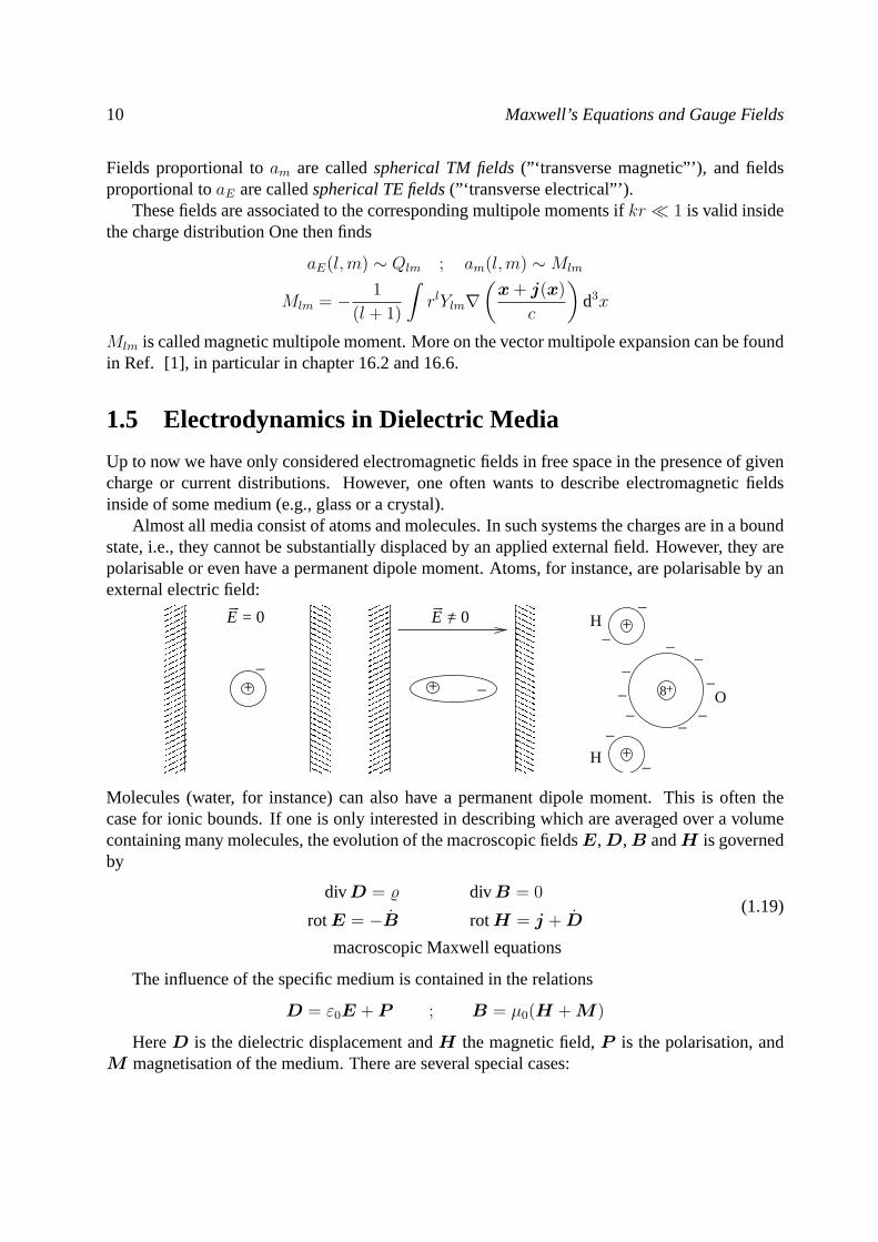
Almost all media consist of atoms and molecules. In such systems the charges are in a boundstate, i.e., they cannot be substantially displaced by an applied external field. However, they arepolarisable or even have a permanent dipole moment. Atoms, for instance, are polarisable by anexternal electric field:
E = 0
+
_
E = 0
+
/
_
+_
_
8+
+ _
_
_
_
__
_
_
__ O
H
H
Molecules (water, for instance) can also have a permanent dipole moment. This is often thecase for ionic bounds. If one is only interested in describing which are averaged over a volumecontaining many molecules, the evolution of the macroscopic fieldsE, D, B andH is governedby
div D = % div B = 0
rotE = −B rotH = j + D(1.19)
macroscopic Maxwell equations
The influence of the specific medium is contained in the relations
D = ε0E + P ; B = µ0(H + M)
HereD is the dielectric displacement andH the magnetic field,P is the polarisation, andM magnetisation of the medium. There are several special cases:
1.6 Macroscopic Maxwell equations 11
• In a vacuum we haveP = 0 andM = 0, leading to the ordinary Maxwell equations.
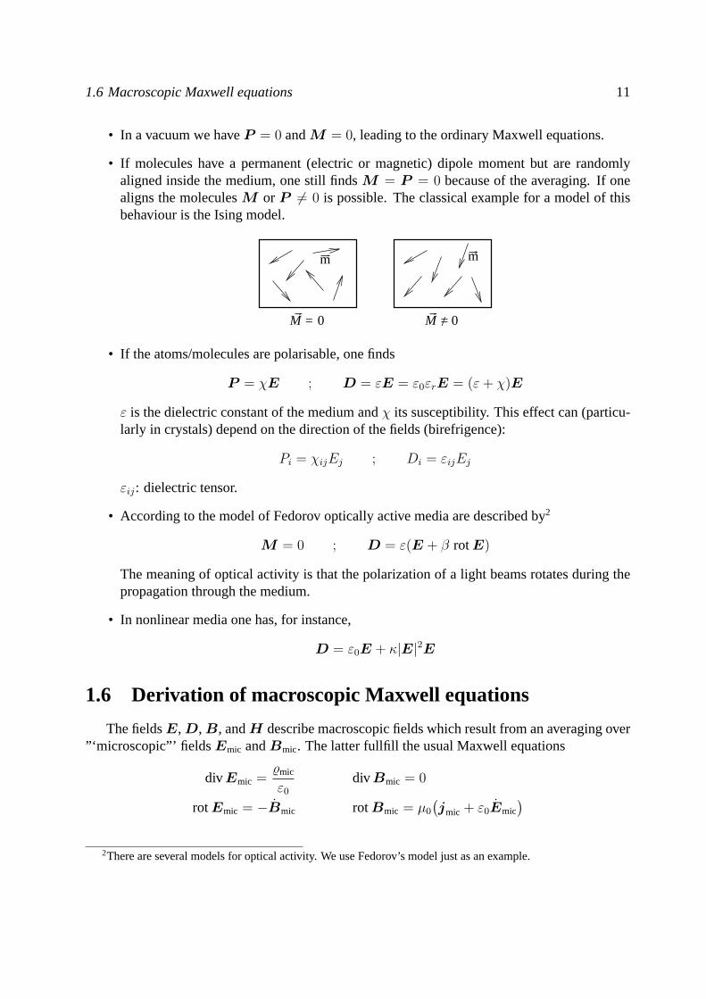
• If molecules have a permanent (electric or magnetic) dipole moment but are randomlyaligned inside the medium, one still findsM = P = 0 because of the averaging. If onealigns the moleculesM or P 6= 0 is possible. The classical example for a model of thisbehaviour is the Ising model.
m m
/M = M = 0 0
• If the atoms/molecules are polarisable, one finds
P = χE ; D = εE = ε0εrE = (ε+ χ)E
ε is the dielectric constant of the medium andχ its susceptibility. This effect can (particu-larly in crystals) depend on the direction of the fields (birefrigence):
Pi = χijEj ; Di = εijEj
εij: dielectric tensor.
• According to the model of Fedorov optically active media are described by2
M = 0 ; D = ε(E + β rotE)
The meaning of optical activity is that the polarization of a light beams rotates during thepropagation through the medium.
• In nonlinear media one has, for instance,
D = ε0E + κ|E|2E
1.6 Derivation of macroscopic Maxwell equations
The fieldsE, D, B, andH describe macroscopic fields which result from an averaging over”‘microscopic”’ fieldsEmic andBmic. The latter fullfill the usual Maxwell equations
div Emic =%mic
ε0
div Bmic = 0
rotEmic = −Bmic rotBmic = µ0
(jmic + ε0Emic
)2There are several models for optical activity. We use Fedorov’s model just as an example.
12 Maxwell’s Equations and Gauge Fields
Charge and current distributions are divided into two parts,
%mic = %free + %bound
jmic = j free + jbound
The free quantities describe particles which are not bound to atoms/molecules. In classical me-chanics their charge distribution can be written as
%free(x) =∑i
qiδ(x− xi)
j free(x) =∑i
qixiδ(x− xi) Sum over free particles.
The bound quantities correspond to the atoms and molecules of the medium.
%bound(x) =∑n
%n(x) Sum over molecules
%n(x) =∑i
qiδ(x− xi) Sum over the particles (e−, nuclei) of the molecule
jbound(x) =∑n
jn(x) ; jn(x) =∑i
qixiδ(x− xi)
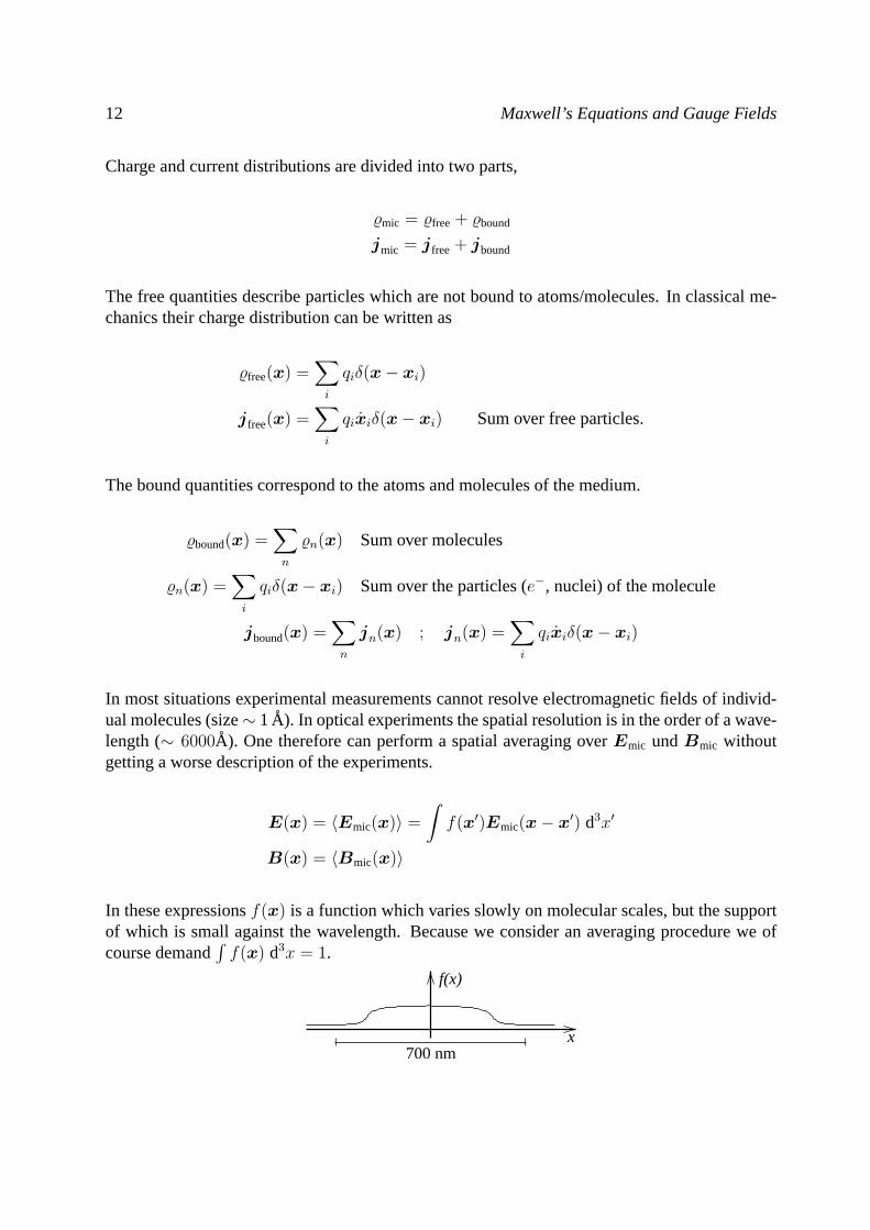
In most situations experimental measurements cannot resolve electromagnetic fields of individ-ual molecules (size∼ 1A). In optical experiments the spatial resolution is in the order of a wave-length (∼ 6000A). One therefore can perform a spatial averaging overEmic undBmic withoutgetting a worse description of the experiments.
E(x) = 〈Emic(x)〉 =
∫f(x′)Emic(x− x′) d3x′
B(x) = 〈Bmic(x)〉
In these expressionsf(x) is a function which varies slowly on molecular scales, but the supportof which is small against the wavelength. Because we consider an averaging procedure we ofcourse demand
∫f(x) d3x = 1.
700 nmx
f(x)
1.6 Macroscopic Maxwell equations 13
The equations forE undB then become
div B(x) =∂
∂xiBi(x)
=∂
∂xi
∫f(x′)Bmic,i(x− x′) d3x′
=
∫f(x′)
∂
∂xiBmic,i(x− x′) d3x′
=
∫f(x′) div Bmic(x− x′)︸ ︷︷ ︸
=0
d3x′
= 〈div Bmic(x)〉 = 0
and analogously divE(x) =〈%mic〉ε0
rotE(x) = −B(x)
rotB(x) = µ0〈jmic(x)〉+1
c2E(x)
The mean values can be calculated as follows.
〈%mic〉 = 〈%free〉+ 〈%bound〉=: %(x) + 〈%bound〉 %(x) : macroscopic charge density
〈%bound〉 =∑
n(molecules)
〈%n(x)〉 (1.20)
The size of each molecule is much smaller than the averaging area. We therefore find
%n(x) ≈∫f(x′)%n(x− x′) d3x′
=
∫f(x′)
∑i(e−, nuclei)
qiδ(x− x′ − xi) d3x′
=∑
i(e−, nuclei)
qif(x− xi) d3x′
If xn is the center of the molecule we have|xi−xn| support off . One therefore can performa Taylor expansion off :
f(x− xi) = f(x− xn − (xi − xn))
≈ f(x− xn)− (xi − xn)∇f(xi − xn) + · · ·
=⇒ 〈%n(x)〉 ≈∑
i(e−, nuclei)
qif(x− xn)− (xi − xn)∇f(xi − xn) + · · ·
=⇒ 〈%n(x)〉 ≈ f(x− xn)∑
i(e−, nuclei)
qi︸ ︷︷ ︸qn
−∇f(x− xn)∑
i(e−, nuclei)
qi(xi − xn) + · · ·︸ ︷︷ ︸pn
14 Maxwell’s Equations and Gauge Fields
qn isthe total charge of thenth molecule. If the molecules are not ionized,qn = 0. pn is themolecule’s dipole moment.
=⇒ 〈%bound〉 =∑
n(molecules)
(−∇f(x− xn)pn
PolarizationP (x) =∑n
f(x− xn)pn ; qn = 0
=⇒ 〈%bound(x)〉 = −div P (x)
Inserting this and Eq. (1.20) into the microscopic Maxwell equations one gets
div E =1
ε0
〈%mic〉
=1
ε0
%− 1
ε0
div P
D = ε0E + P =⇒ div D = %
A similar treatment of
rotB = µ0〈jmic〉+1
c2E
leads to
〈jmic〉 = j + rotM + P
M = 〈∑n
mnδ(x− xn)〉
mn =∑
i(e−, nuclei)
qi2mi
(xi ×mixi) =∑
i(e−, nuclei)
qi2mi
Li
Heremn denotes the magnetic dipole moment of thenth molecule. (details can be found in [1],section6.7). This concludes the derivation of the macroscopic Maxwell equations Eq. (1.19).
1.7 Plane Waves
In vacuum (% = j = 0) the following relations hold,
E = B = 0 ; div E = div B = 0
Ansatz for solution:
E = Ekεk exp(ikx− iωt)
E = Ekεk
(1
c2∂2
∂t2−∆
)exp(ikx− iωt)
1.7 Plane Waves 15
where Ek ∈ C is the amplitude andεk the polarisation vector.
=⇒ E = Ekεk(−ω2
c2+ k2) exp(ikx− iωt)
!= 0
This is a solution ofE = 0 if ω = c|k|, whereωk := c|k| is the frequency of a photon3 withmomentum~k. Its energy is given by Planck’s equationE = ~ωk. The polarisation vectorεk isdetermined by the condition divE = ∂iEi = 0:
div E = Ek(εk)iiki exp(ikx− iωkt)
= iEk(εkk) exp(ikx− iωkt)
!= 0
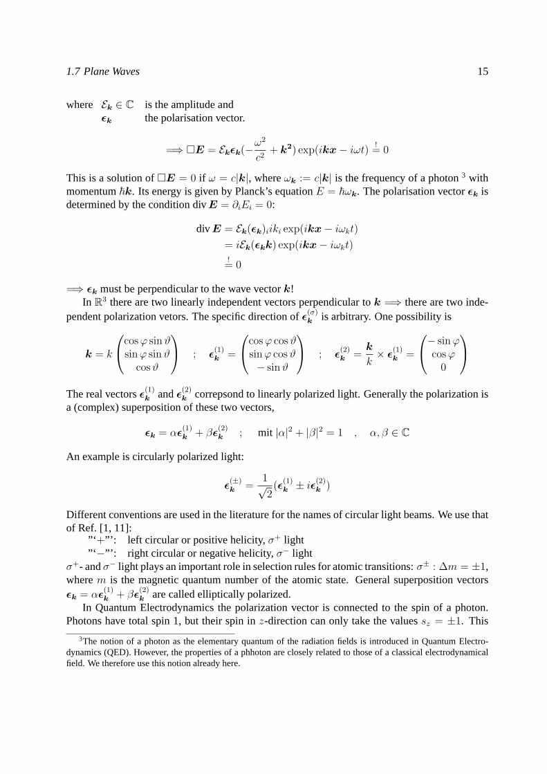
=⇒ εk must be perpendicular to the wave vectork!In R3 there are two linearly independent vectors perpendicular tok =⇒ there are two inde-
pendent polarization vetors. The specific direction ofε(σ)k is arbitrary. One possibility is
k = k
cosϕ sinϑsinϕ sinϑ
cosϑ
; ε(1)k =
cosϕ cosϑsinϕ cosϑ− sinϑ
; ε(2)k =
k
k× ε
(1)k =
− sinϕcosϕ
0
The real vectorsε(1)
k andε(2)k correpsond to linearly polarized light. Generally the polarization is
a (complex) superposition of these two vectors,
εk = αε(1)k + βε
(2)k ; mit |α|2 + |β|2 = 1 , α, β ∈ C
An example is circularly polarized light:
ε(±)k =
1√2(ε
(1)k ± iε
(2)k )
Different conventions are used in the literature for the names of circular light beams. We use thatof Ref. [1, 11]:
”‘ +”’: left circular or positive helicity,σ+ light”‘−”’: right circular or negative helicity,σ− light
σ+- andσ− light plays an important role in selection rules for atomic transitions:σ± : ∆m = ±1,wherem is the magnetic quantum number of the atomic state. General superposition vectorsεk = αε
(1)k + βε
(2)k are called elliptically polarized.
In Quantum Electrodynamics the polarization vector is connected to the spin of a photon.Photons have total spin 1, but their spin inz-direction can only take the valuessz = ±1. This
3The notion of a photon as the elementary quantum of the radiation fields is introduced in Quantum Electro-dynamics (QED). However, the properties of a phhoton are closely related to those of a classical electrodynamicalfield. We therefore use this notion already here.
16 Maxwell’s Equations and Gauge Fields
corresponds toσ+- andσ− light. The selection rule∆m = ±1 is then simply a consequenceof angular momentum conservation when the atom absorbs a photon. The valuesz = 0 is notrealized in nature because of the vanishing rest mass of photons (see, e.g., Ref. [9], section 14.5).The magnetic field of a plane wave can be derived from the electric field with the aid of theMaxwell equation rotE = −B:
B = −rot Ekεke(ikx−iωkt) + c.c.
= −εijk∂j(εk)lEke(ikx−iωkt) + c.c.
= −εijk(εk)lEklkje(ikx−iωkt) + c.c.
= −iEk(k × εk)ie(ikx−iωkt) + c.c.
To solve this we setBi ∼ exp(−iωkt). We then find
B =Ek
ωk(k × εk)e(ikx−iωkt) + c.c.
=1
ωk(k ×E)
The general solution in free space is a superposition of plane waves
E(x, t) =
∫d3k
∑σ=1,2
E (σ)k ε
(σ)k exp(ikx− iωt) + c.c.
B(x, t) =
∫d3k
∑σ=1,2
E (σ)k
ωk(k × ε
(σ)k ) exp(ikx− iωt) + c.c.
The following special cases are worth to be mentioned:
1. The polarization vector is composed of a real partε and a imaginary partε′′,
E = Ekεk exp(ikx− iωkt) + c.c.
= Ek(ε′ + iε′′) exp(ikx− iωkt) + c.c.
where we assumeε′2 + ε′′2 = 1, E ∈ R.
=⇒ E = Ekε′2 cos(kx− iωkt)− Ekε′′2 sin(kx− iωkt)
This is a running wave.
2. Consider a superposition of two counter-propagating waves withEk = E−k undεk = ε−k:
E = Ek + E−k
= Ekεk exp(ikx− iωkt) + E−kε−k exp(−ikx− iωkt) + c.c.
=⇒ E ∼ cos(kx)cos(ωkt)
This is a standing wave.
Chapter 2
Quantum Field Theory of Light - QED
2.1 Many-Particle Theory of Quantum Mechanics
We assume that the reader is familiar with the Schrodinger equation for a single particle. If oneconsiders two non-interacting free particles, the Hamiltonian is given by the sum of the individualHamiltonians,
H =p2
1
2m+
p22
2m(2.1)
The corresponding two-particle wavefunction has the form
ψ (x1,x2) = φn (x1) · φm (x2) (2.2)
In this wavefunction the particles are distinguishable (through their quantum numbersn, m).However, experiments demonstrate that identicaluarticles are NOT distinguishable. In the the-oretical description this is guaranteed ifψ(x1,x2) leads to the same measurement results asψ(x2,x1). To examine this more closely we introduce the exchange operatorE,
Eψ(x1,x2) = ψ(x2,x1) (2.3)
Because ofE2 = 1 the eigenvalues of the exchange operator are±1. The corresponding eigen-functions fullfill
EψB(x1,x2) = +ψB(x1,x2) = ψB(x2,x1) (2.4)
EψF (x1,x2) = −ψF (x1,x2) = ψF (x2,x1) (2.5)
All experimental results indicate that all particles in nature are eigenstates ofE:
• ψB ⇔ Bosons
• ψF ⇔ Fermions
The well-known Pauli principle for Fermions is a direct consequence of the antisymmetry ofψF .
18 Quantum Field Theory of Light - QED
Spin-Statistics Theorem
• Bosons⇔ interger spin
• Fermions⇔ half-integer spin
The proof of this theorem essentially relies on causality and can be found in Ref. [5].
Many-particle Wavefunction ψ(x1, . . . , xn) should be symmetric or antisymmetric under ex-change of any pair of particles:
ψ(x1, . . . , xi, . . . , xj, . . . , xn) = ±ψ(x1, . . . , xj, . . . , xi, . . . , xn) (2.6)
This can be achieved by symmetrization: sum over all permutations and normalize
ψB (x1, . . . , xn) =1√N !
∑p
ψ(xp(1), . . . , xp(n)
)(2.7)
ψF (x1, . . . , xn) =1√N !
∑p
(−1)pψ(xp(1), . . . , xp(n)
)(2.8)
wherebyp characterizes the permutation:(−1)p = 1 for an even number of exchanges, and−1for an odd number of exchanges.
As an example we use the product wavefunction of free particles,
ψ(x1, x2, x3) = ψl(x1)ψm(x2)ψn(x3) , (2.9)
i.e., particle 1 in state l, particle 2 in state m, and particle 3 in state n. This means that the particleare distinguishable.
For Fermions the corresponding indistinguishable wavefunction is
ψFlmn(x1, x2, x3) =1√6ψl(x1)ψm(x2)ψn(x3)− ψl(x2)ψm(x1)ψn(x3)
+ψl(x2)ψm(x3)ψn(x1)− ψl(x3)ψm(x2)ψn(x1)
+ψl(x3)ψm(x1)ψn(x2)− ψl(x1)ψm(x3)ψn(x2)
For a large number of particles this procedure becomes rather tedious.
2.1.1 Fock Space and Number Representation
In single-particle quantum mechanics we usually do not need to know the full wavefunctionψ(x)in position space. To completely fix the state it is sufficient to know a complete set of quantumnumbers. For the hydrogen atom, for instance, these are the quantum numbers n,l and m (ignoringspin). To know the state it is sufficient to specify|n, l,m〉 instead ofψnlm(x) = 〈x|n, l,m〉.
2.1 Many-Particle Theory of Quantum Mechanics 19
Likewise, in many-particle quantum mechanics it is sufficient to know, how many particlesare in a state: the ket|1l, 1m, 1n〉 can unambiguously be associated with the state ”one particle instate l, one in m, one in n”, i.e., with the wavefunctionψFlmn(x1, x2, x3).
Example for Bosons:
ψBllm(x1, x2, x3) =1√3ψl(x1)ψl(x2)ψm(x3)
+ψl(x1)ψl(x3)ψm(x2)
+ψl(x2)ψl(x3)ψm(x1)⇐⇒ |2l, 1m〉
Superposition of such states are possible and can also be prepared in an experiment. Example
|ψ〉 = α |2l, 1m〉+ β |3l, 0m〉+ γ |1l, 2m〉
However, also superpositions of states with a different number of particles, like
|ψ〉 = α |1l〉+ β |2l〉+ γ |3l, 4m〉 . . . ,
are possible. Formally superpositions of states with different particle numbers are an element ofFock space, which is defined as follows:
• LetH(1) be the Hilbert space for 1-particle wavefunctions
• H(2) = Hilbert space for 2-particle wavefunctions . . .
Fock space is the direct sum of all N-particle Hilbert spaces:
F := H(0) ⊕H(1) ⊕H(2) ⊕ · · · ⊕ H(N) (2.10)
H(0) describes the vacuum and correspondingly includes only a single state, denoted by|0〉(〈0|0〉 = 1).
Fock space is needed to describe processes in which the number of particles is not coserved.For instance, pair production ofe+ ande− from aγ photon is described by1
|1γ〉 ⊗ |0e+〉 |0e−〉 −→ |0γ〉 ⊗ |1e+〉 |1e−〉
A second example is the excitation of one atom from the ground state|1g〉 to the excited state|1e〉 by absorbing a photon:
|1g〉 ⊗ |1γ〉 −→ |1e〉 ⊗ |0γ〉
1Actually an additional particle is needed to make energy and momentum conservation possible. However, herewe are only interested in the underlying principle.
20 Quantum Field Theory of Light - QED
2.1.2 Creation and Anihilation Operators
These two types of operators allow a simple representation of many-particle wavefunctions. Thecreation operatora†l for a particle in statel (also called model) and the corresponding anihilationoperatoral are defined by
a†l |n(l)l , n
(m)m . . .〉 =
√n(l) + 1 |(n(l) + 1)l, n
(m)m . . .〉 (2.11)
al |n(l)l , n
(m)m . . .〉 =
√n(l) |(n(l) − 1)l, n
(m)m . . .〉 (2.12)
These are the definitions for Bosons.These operators fullfill the following commutation relations (For simplicity we omit the in-
dices). [a†, a
]|n〉 = a†a |n〉 − aa† |n〉
= a†√n |n− 1〉 − a
√n+ 1 |n+ 1〉
= n |n〉 − (n+ 1) |n〉= (−1) |n〉
This implies[a, a†
]= 1. The action of these operators is equivalent to the corresponding opera-
tors for the harmonic oscillator. The general commutation relations are[al, a
†m
]= δlm (2.13)
[al, am] =[a†l , a
†m
]= 0 (2.14)
The physical reason for this close analogy to the harmonic oscillator is that the energy levels offree particles in one mode have the same structure: the creation ofn particles each with energyE0 corresponds to a total energynE0. This corresponds to ann-fold excitation of a harmonicoscillator of energyE0 = ~ωObviously one finds for Bosons
a†lH(N) −→ H(N+1)
alH(N) −→ H(N−1)
al |0〉 = 0 = Number!
Here the first two equations define a mapping from Fock space into Fock space. The last equationdefines the vacuum state and essentially states that one cannot anihilate a particle if there is none.
Because of Pauli’s principle it is not possible to have two Fermions in the same state. There-fore, the Fermion creation operators need to fullfill(a†l )
2 = 0. This can be achieved through theanticommutation relations
a†l , a†m = al, am = 0 al, a†m = δlm (2.15)
where the anticommutator is defined byA,B := AB +BA.
2.1 Many-Particle Theory of Quantum Mechanics 21
2.1.3 The Field Operator
How can one calculate expectation values using creation operators? Let us first consider anordinary 1-particle operatorO(x, p). In the theory of a single particle one has
〈O〉 =
∫ψ∗(x)Oψ(x)d3x
If we have N particles in this state the expectation value ofO is of course given by
〈O〉 =N∑i=1
〈O〉1-particle
This suggests to define the expectation value of a 1-particle operator in the framework of many-particle theory as follows,
〈ON〉 :=N∑i=1
〈 O(xi, pi) 〉
=N∑i=1
∫d3x1 . . . d
3xn ψ∗N(x1, . . . xN)ONψ(x1, . . . xn) (2.16)
Consider for instance the energy and the corresponding equations for the eigenvalues,
H(x, p)ψa(x) = Eaψa(x) (2.17)
For an-particle state|na, . . . , na′ , . . . , na′′〉 the energy is given by
E = Eana + . . .+ Eana′ + . . . (2.18)
=
∫d3x ψ∗a(x)H(x, p)ψa(x)na +
∫d3x ψ∗a′(x)H(x, p)ψa′(x)na′ + . . .
The particle numbersna, na′ , . . . can be calculated with the aid of creation/anihilation operators.To do so we introduce the operator
Na = a†aaa (2.19)
This is the Number operator for particles in statea. Its physical meaning is revealed by thefollowing calculation.
〈. . . , na, . . . |Na| . . . , na, . . .〉 = 〈. . . , na, . . . |a†aaa| . . . , na, . . .〉 (2.20)
= 〈. . . , na, . . . |a†a√na| . . . , (na − 1)a, . . .〉
= 〈. . . , na, . . . |√
(na − 1) + 1√na| . . . , na, . . .〉 = na 〈. . . | . . .〉 = na
22 Quantum Field Theory of Light - QED
And therefore we have forE:
E =
∫d3x ψ∗a(x)H(x, p)ψa(x) 〈. . . , na, . . . , na′|a†aaa| . . . , na, . . . , na′〉 (2.21)
+
∫d3x ψ∗a′(x)H(x, p)ψa′(x) 〈. . . , na, . . . , na′|a†a′aa′| . . . , na, . . . , na′〉
+ . . .
Important:
In this expression the operatorsaa, a†a do only act on the many particle states, not onthe wavefunctionψa(x).Contrarywise,H(x, p) acts only onψa(x) but not on|. . . , na, . . .〉.The number representation of many-particle states can be considered as a kind ofbookkeeping procedure to simplify the combinatorics associated with the symmetriza-tion/antisymmetrization of many-particle states.
We therefore can rewrite the expression forE as
E = 〈. . . , na, na′ , . . . |∫d3x ψ∗a(x)H(x, y)ψa(x)a
†aaa| . . . , na, na′ , . . .〉+ . . . (2.22)
Thefield operatoris defined byΨ(x) :=∑
a aaψa(x) and allows us to rewrite the mean energyas
E = 〈. . . , na, na′ , . . . |∫d3x Ψ†(x)H(x, y)Ψ(x)| . . . , na, na′ , . . .〉 (2.23)
Proof:
〈. . . |∫d3x Ψ†HΨ| . . .〉 = 〈. . . |
∫d3x
∑a
ψ∗a(x)a†aH∑b
ψb(x)ab| . . .〉 (2.24)
=∑a,b
∫d3x ψ∗aHψb︸ ︷︷ ︸
=Eb
Rψ∗aψb=Ebδab
〈. . . |a†aab| . . .〉 =∑a
Ea 〈. . . |a†aaa| . . .〉 =∑a
Eana = E
One generally can express the expectation value of any 1-particle operatorO(x, p) in a Fock state|ψ〉 by
〈O(x, p)〉 = 〈ψ|∫d3x Ψ†(x)O(x, p)Ψ(x)|ψ〉 (2.25)
This holds for any state in Fock space, e.g.,
|ψ〉 = |1a〉+ |2a′〉 → 〈ψ|Ψ†Ψ|ψ〉 = 〈1a|Ψ†Ψ|1a〉+ 〈2a′|Ψ†Ψ|2a′〉 (2.26)
Remarks on the field operator:
2.1 Many-Particle Theory of Quantum Mechanics 23
• In a sense,Ψ(x) is both an operator and a 1-particle state:
Ψ(x) =∑a
aaψa(x) (2.27)
aa: Operator in Fock spaceψa(x): 1-particle stateOne could (and sometimes does) writeψa(x) as〈x|ψa〉1-particle
→ Ψ(x) = 〈x|∑
aa|ψa〉Eint.
= 〈x|Ψ〉Eint. (2.28)
• Interpretation ofΨ(x): What is the meaninf of the stateΨ†(x) |0〉? In the following wewill see that it is a very special 1-particle state. To see this we first consider a perfectlylocalized state inH(1) (actually, perfectly localized states are not normalizable, but thisdoesn’t matter for us):
φx0(x) = δ(x− x0) =∑n
cnφn(x), φn= basis ofH(1)
cn =
∫d3x φ∗n(x)φx0(x) =
∫d3x φ∗n(x)δ(x− x0) = φ∗n(x0)
→ φx0(x) =∑n
φ∗n(x0)φn(x) (completness relation) (2.29)
The Fock-space representation of this state is given by∑n
φ∗n(x0) |1n〉 =∑n
φ∗n(x0)a†n |0〉 = Ψ†(x0) |0n〉 (2.30)
Thus,Ψ†(x0) createsa particle at the positionx0.Ψ(x0) anihilatesa particle at the positionx0.
• Commutation relations for Bosons:[Ψ(x),Ψ†(x)
]=
[∑l
alψl(x),∑n
a†nψ∗n(y)
]=∑l,n
ψl(x)ψ∗n(y) [al, a
†m]︸ ︷︷ ︸
δln
=∑n
ψn(x)ψ∗n(y) = δ(x− y) (for Bosons) (2.31)
[Ψ(x),Ψ†(y)
]= δ(x− y) (2.32)[
Ψ†(x),Ψ†(y)]
= [Ψ(x),Ψ(y)] = 0 (2.33)
For Fermions we have analogously
al, a†m = δlm = ala†m + ama
†l
→Ψ(x),Ψ†(y)
= δ(x− y) (2.34)
Ψ†(x),Ψ†(y)
= Ψ(x),Ψ(y) = 0 (2.35)
24 Quantum Field Theory of Light - QED
2.1.4 Second Quantization
The construction of field operators described above is mathematically equivalent to a secondquantization procedure applied on the Schrodinger wavefunction.Canonical quantization of a classical particle:Using the Lagrange functionL(x, x) one can define the canonical momentum by
p =∂L
∂x(2.36)
Quantization is achieved by re-interpretingx andp as operators and demanding the commutationrelations
[x, p] = i~ (2.37)
The same procedure can be done for a field:For a Schrodinger particle one can introduce the Lagrange density
L(ψ, ψ∗, ψ, ψ∗) = i~(ψ∗ψ − ψ∗ψ)− ~2
2m∇ψ∗∇ψ − ψ∗V ψ (2.38)
The Euler-Lagrange equation for this Lagrangean leads to the complex conjugate of the Schrodingerequation,
∂t∂L∂ψ
= −∂i∂L
∂(∂iψ)+∂L∂ψ
(2.39)
→ ∂ti~ψ∗ = ∂2i
~2
2mψ∗ − V ψ∗ (2.40)
One can define the canonically conjugate momentum density by
π(x) =∂L
∂ψ(x)= i~ψ∗(x) (2.41)
If one applies again the canonical quantization scheme one finds
ψ(x), π(x) → Ψ(x),Π(x)
[Ψ(x),Π(y)] = i~δ(x− y) →[Ψ(x),Ψ†(y)
]= δ(x− y) (2.42)
This means that, by applying the canonical quantization procedure a second time, we end up withthe same commutation relations as that derived from the construction of the field operator fromcreation/anihilation operators.
The method of second quantization is most popular method used to construct a many-particletheory of fields. However, it has the disadvantage that the construction of Fock space and themeaning of the field operator is not as obvious as in the previous procedure.
2.1 Many-Particle Theory of Quantum Mechanics 25
2.1.5 Summary of the construction of a many-particle theory
Recipe to construct a many-particle theory (quantum field theory) using the example of theSchrodinger field:
(i) Choose stationary solutionsϕn(x) of a 1-particle theory with〈ϕn|ϕm〉 = δnm. Te scalarproduct should be time-independent since otherwise the meaning of the modes, and there-fore of the creation and annihilation operators, would be time-dependent. The interpreta-tion of operators in Schrodinger picture would then be more difficult.
i~∂tψ = Hψ, 〈ψ|ψ′〉 =
∫d3x ψ∗ψ′
∂t 〈ψ|ψ′〉 =
∫ (ψ∗ψ′ + ψ∗ψ′
)d3x =
∫ i
~(Hψ∗)ψ′ + ψ∗
−i~Hψ′)
d3x
=i
~
∫ψ∗(Hψ′)− ψ∗(Hψ′) = 0 (2.43)
where we have used the hermitean conjugate Schrodinger equation and the hermiticity ofH with respect to the scalar product.
(ii) Replace the general solution of the 1-particle equations of motion,
ψ(x) =∑n
cnϕn(x) , (2.44)
by the field operator
Ψ(x) =∑n
anϕn(x) mit[an, a
†m
]= δnm (2.45)
(an, a†m = δnm for Fermions, respectively).Ψ†(x) creates a particle at positionx.
2.1.6 Quantization in Coulomb Gauge
The Lagrangean densityL of the electromagnetic field is given by
L ∝ E2 − c2B2 = (−∇φ− A)2 − c2(rotA)2 (2.46)
L does not depend on derivatives of the fieldsE and B. It therefore does only lead toMaxwell’s equations if it is considered as a function of the potentials. The field equations inCoulomb gauge (divA = 0) are
A = µ0j −1
c2∇φ, ∆φ = − %
ε0(2.47)
The equation forφ is not dynamical!
26 Quantum Field Theory of Light - QED
In vacuum the corresponding equations read
A = − 1
c2∇φ, ∆φ = 0 (2.48)
Boundary conditions: φr→∞−→ 0 =⇒ φ = 0 =⇒ A = 0
Solution:
A(x, t) = A(+)(x, t) + A(−)(x, t) (2.49)
=
∫d3k
∑σ=1,2
Akσ
modefunction︷ ︸︸ ︷εεσkNσk exp (−iωkt) exp (ikx)︸ ︷︷ ︸
A(+)(x, t)
+ c.c.︸︷︷︸A(−)(x, t)
(2.50)
Here we have introduced
• the expansion coefficientsAkσ
• the polarization vectorsεεσk
• the normalization coefficientsNσk
• A(+)(x, t) denotes the so-called”positive frequency part“ (∝ exp (−iωkt)) which only
contains anihilation operators.
We know thateikx is a complete basis (because of Fourier transformation, and leaving asideissues of normalization). Since all possible factors ofeikx already appear inA(+)(x, t), it issufficient to consider onlyA(+)(x, t). Since the classical fieldA(x, t) is real, the correspondingquantum field operatorA must be hermitean. Because of[a, a†] = 1 it is clear thata cannot behermitean. Thus, the full operatorA cannot be composed out of anihilation operators alone. Thisis another (and more important) reason to useA(+)(x, t) instead ofA(x, t) for the quantizationprocedure.
Let nowA(+)(x, t) andA′(+)(x, t) be solutions ofA = 0. A conserved scalar product isthen given by⟨
A(+)(x, t)∣∣∣A′(+)(x, t)
⟩= −iε0
∫d3x A
(+)∗︸ ︷︷ ︸A
(−)
A′(+) −A(+)∗︸ ︷︷ ︸A(−)
A′(+)
The prefactor appears out of dimensional considerations:
[A] =Js
Cm=⇒ [〈A |A′ 〉] = 1
2.1 Many-Particle Theory of Quantum Mechanics 27
Proof of time-independence of the scalar product:
∂t〈A|A〉 = −iε0
∫d3x
A∗A′ + A
∗A′ − A
∗A′ −A∗A′
!= 0
use1
c2A−∆A = 0
=⇒ ∂t〈A|A〉 = −iε0c2∫
d3x (∆A∗) A′ −A∗ (∆A′)
= −iε0c2∫
d3x A∗ (∆A′)− (∆A∗) A′
= 0
whereweused
∫ (∇i∇iA
∗j
)A′
j = −∫∇iA
∗j∇iA
′j =
∫A∗j∇i∇iA
′j
Normalization of plane wavesNkσεεkσ exp (ikx− iωkt) = ϕkσ(x, t)
〈ϕkσ|ϕk′σ′〉!= δσσ′δ(k − k′)
= −iε0
∫d3xNkσNk′σ′εε
∗kσεεk′σ′
e−ikxeiωkt (iωk) eik′xe−iωk′ t
−e−ikxeiωkt (−iωk′) eik′xe−iωk′ t
with
∫d3x ei(k−k′)x = (2π)3δ(k − k′) it follows that
〈ϕkσ|ϕk′σ′〉 =ε0
(2π)3 εε∗kσεεkσ′︸ ︷︷ ︸δσ,σ′
δ(k − k′) NkσNkσ′ 2ωk
=ε0
(2π)32ωk N2kσδσ,σ′δ(k − k′)
!= δσ,σ′ δ(k − k′)
=⇒ Nkσ =
√
2(2π)3ε0ωk
for t = 0 it follows that2 for A(x):
A(x) =
∫d3k
∑σ
Akσ
√
2(2π)3ε0ωkεεkσ exp (ikx) + c.c. (2.51)
2We sett = 0 to derive the time-independent vector potential operator in Schrodinger picture. One can alsoconsidert 6= 0 to derive the corresponding operator in interaction picture.
28 Quantum Field Theory of Light - QED
Quantization: replace the amplitudeAkσ by the anihilation operatorakσ with
[akσ, a
†k′σ′
]= δσ,σ′ δ(k − k′)
a†kσ creates a photon ( = quantum of light ) with momentumk and polarization vectorεεkσ .In contrast to the classical theory of electromagnetism, intensity and energy of a light beam ap-pear in quantized portions.
Photons are Bosons and have spin 1, but they have onlytwo possible values for the magneticquantum number,m = +1,−1. These values correspond to left- and right-circularly polarizedplane waves. m = 0 (⇒ longitudinally polarized photons⇔ εεkσ ‖ k ) is not possible because ofthe vanishing mass of photons (see, e.g., Sec. 14.5 of Ref. [9]).
The operators for the electric and magnetic field can easily be derived from that for the vectorpotential:
E(x)∣∣∣t=0
= − ˙A(x)
∣∣∣t=0
= i
∫d3k
∑σ
akσ
√ωk
2(2π)3ε0εεkσe
ikx + H.c. (2.52)
B(x) = rotA(x) = i
∫d3k
∑σ
akσ
√
2(2π)3ε0ωk(k × εεkσ)e
ikx + H.c. (2.53)
The Hamiltonian can be found using the classical expression for the energy density:
H =ε02
∫d3x
(E
2(x) + c2B
2(x))
= . . .
=
∫d3k
∑σ
ωk2
a†kσakσ + akσa
†kσ
=
∫d3k
∑σ
ωka†kσakσ +
1
2
(2.54)
(⇔ sum over harmonic oscillators)
The Heisenberg equations of motion for operators (in Heisenberg picture) are generally givenby
i∂tO(t) =[O(t), H
](2.55)
2.1 Many-Particle Theory of Quantum Mechanics 29
so that we can deduce
iEi(x, t) =
[Ei(x, t),
∫d3k
∑σ
ωka†kσakσ +
1
2
]
= i
∫d3k′
∑σ′
√ωk′
2(2π)3ε0[ak′σ′ e
ik′x(εεk′σ′)i − a†k′σ′e−ik′x(εε∗k′σ′)i,
∫d3k
∑σ
ωka†kσakσ +
1
2
]
= i
∫d3k′
∑σ′
∫d3k
∑σ
√ωk′
2(2π)3ε0ωk
eik′x(εεk′σ′)iδ(k − k′)δσσ′akσ − e−ik
′x(εε∗kσ′)ia†k′σ′(−δσσ′δ(k − k′))
=⇒ E =
∫d3k
∑σ
ω2k
√
2(2π)3ε0ωk
(akσe
ikxεεkσ + a†kσe−ikxεε∗kσ
)(2.56)
Let us now calculate(rotB)i:
(rotB)i = i
∫d3k
∑σ
εijl∂
∂xjakσ(k × εεkσ)le
ikx
√~
2(2π)3ε0ωk
− i
∫d3k
∑σ
εijl∂
∂xja†kσ(k × εε∗kσ)le
−ikx
√~
2(2π)3ε0ωk
rotB = −∫
d3k∑σ
√~
2(2π)3ε0ωk
(k × (k × εεkσ)akσe
ikx + k × (k × εε∗kσ)a†kσe−ikx
)(2.57)
With k · εεkσ = 0 we also find
k × (k × εεkσ) = k(k · εεkσ)− εεkσk2 = −εεkσk
2 (2.58)
so that
rotB =
∫d3k
∑σ
√~
2(2π)3ε0ωkk2akσeikxεεkσ + a†kσe
−ikxεε∗kσ (2.59)
⇒ rotB =1
c2E = µ0ε0E (2.60)
This is one of the inhomogeneous Maxwell equations forj = 0 (otherwise we have rotB =1c2
E = µ0j + ε0E). Analogously one can show that
i~B = [B, H] = . . .
30 Quantum Field Theory of Light - QED
⇒ B = −rotE (2.61)
Becausek · εεkσ = k · (k × εεkσ) = 0div B = 0 (2.62)
and
div E = 0
(=
%
ε0
)(2.63)
⇒ The field operators fullfill Maxwell’s equations in a vacuum
The equations of motions are easily solved if one considers the indivisual modes,
i~akσ = [akσ, H]
=
akσ,∫ d3k′∑σ′
~ω′
k
(a†k′σ′
ak′σ′ +1
2
)=
∫d3k
′∑σ′
~ωk′δσσ′δ(k − k′)ak′σ′
= ~ωkakσ (2.64)
The solution isakσ = e−iωktakσ(0)
whereakσ(0) is the Schrodinger operator for the corresponding mode Mode. The solution hasthe same structure as the respective classical wave.
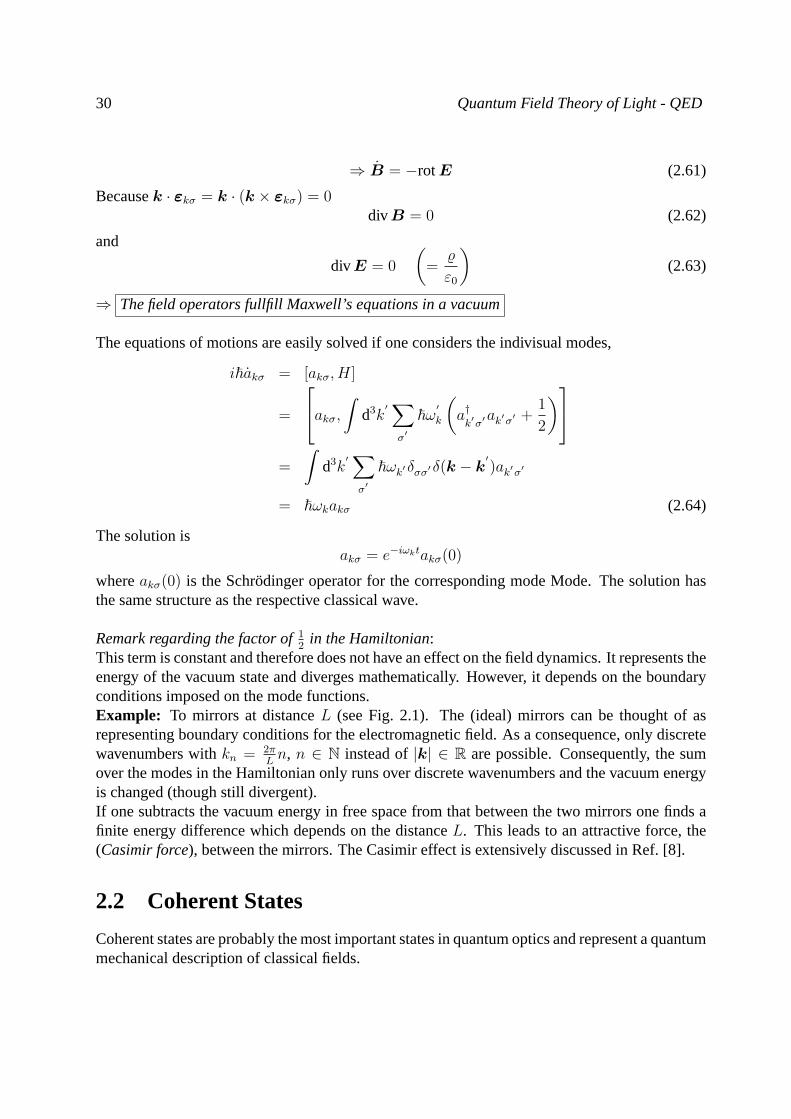
Remark regarding the factor of12
in the Hamiltonian:This term is constant and therefore does not have an effect on the field dynamics. It represents theenergy of the vacuum state and diverges mathematically. However, it depends on the boundaryconditions imposed on the mode functions.Example: To mirrors at distanceL (see Fig. 2.1). The (ideal) mirrors can be thought of asrepresenting boundary conditions for the electromagnetic field. As a consequence, only discretewavenumbers withkn = 2π
Ln, n ∈ N instead of|k| ∈ R are possible. Consequently, the sum
over the modes in the Hamiltonian only runs over discrete wavenumbers and the vacuum energyis changed (though still divergent).If one subtracts the vacuum energy in free space from that between the two mirrors one finds afinite energy difference which depends on the distanceL. This leads to an attractive force, the(Casimir force), between the mirrors. The Casimir effect is extensively discussed in Ref. [8].
2.2 Coherent States
Coherent states are probably the most important states in quantum optics and represent a quantummechanical description of classical fields.
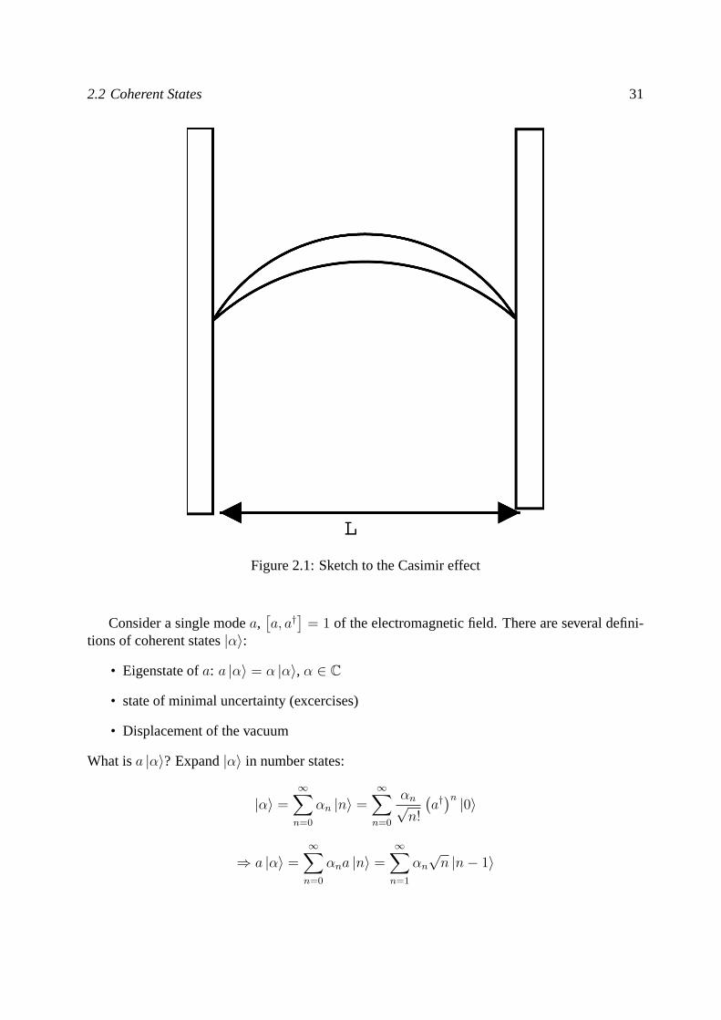
2.2 Coherent States 31
Figure 2.1: Sketch to the Casimir effect
Consider a single modea,[a, a†
]= 1 of the electromagnetic field. There are several defini-
tions of coherent states|α〉:
• Eigenstate ofa: a |α〉 = α |α〉, α ∈ C
• state of minimal uncertainty (excercises)
• Displacement of the vacuum
What isa |α〉? Expand|α〉 in number states:
|α〉 =∞∑n=0
αn |n〉 =∞∑n=0
αn√n!
(a†)n |0〉
⇒ a |α〉 =∞∑n=0
αna |n〉 =∞∑n=1
αn√n |n− 1〉
32 Quantum Field Theory of Light - QED
With n′ = n− 1 one finds
a |α〉 =∞∑n′=0
αn′+1
√n′ + 1 |n′〉 !
= α |α〉 = α∞∑n′=0
αn′ |n′〉
It follows thatαn+1 = α αn√n+1
, wherebyα0 has to be fixed by the normalization condition. From
α1 = αα0
α2 =α2
√2!α0
α3 =α3
√3!α0 etc.
one can deduce
αn =αn√n!α0 (2.65)
This results in
|α〉 = α0
∞∑n=0
αn√n!|n〉 = α0
∞∑n=0
αn
n!
(a†)n |0〉 = α0 exp
(αa†)|0〉
Using〈n|m〉 = δnm and Eq. (2.65) one is led to
〈α|α〉 = 1 = |α0|2∞∑n=0
(α∗)n√n!〈n|
∞∑m=0
αm√m!|m〉 = |α0|2
∞∑n=0
|α|2n
n!= |α0|2 exp |α|2 !
= 1
This leads to
α0 = exp
(−|α|
2
2
)(2.66)
We thus can represent the coherent state|α〉 as
|α〉 = exp
(−|α|2
2
) ∞∑n=0
αn√n!|n〉 = exp
(−|α|
2
2
)exp(αa†) |0〉 (2.67)
|α〉 can also be constructed using thedisplacement operator
D(α) = exp (αa† − α∗a) . (2.68)
To do so we can use the Baker-Campbell-Hausdorf equation:
e(A+B) = eAeBe−12[A,B]e−
16[A,[A,B]] . . . (2.69)
InsertingA = αa† andB = −α∗a we find
−1
2[A,B] = −1
2(−|α|2)[a†, a] = −|α|
2
2∈ R
2.2 Coherent States 33
⇒ [A, [A,B]] = 0
Together with Eq. (2.69) the then can be brought into the form
D(α) = eαa†e−α
∗ae−|α|22 (2.70)
This allows us to prove the following properties of the displacement operator:
• D(α) is unitary:
D†(α) = eα∗a−αa† = e−(αa†−α∗a) = D−1(α) = D(−α)
• We have the relation|α〉 = D(α) |0〉 (2.71)
It becomes clear from Eq. (2.71) that the vacuum can be considered as the special coherentstateα = 0.
It was shown in the excercises that3
E ∼ a+ a† (2.72)
B ∼ i(a† − a) (2.73)
Thus,
E = 〈α|E |α〉 = 〈α| a+ a† |α〉 = α+ α∗ = 2Reα (2.74)
B = 〈α|B |α〉 = 〈α| i(a† − a) |α〉 = i(α∗ − α) = 2Imα (2.75)
(∆E)2 = 〈E2〉 − E2
= 〈α| a2 + aa† + a†a+ (a†)2 |α〉 − (α− α∗)2
= α2 + (α∗)2 + α∗α+ 〈α| aa† |α〉 − (α− α∗)2
= α2 + (α∗)2 + α∗α+ 〈α| a†a+[a, a†
]|α〉 − (α− α∗)2
= α2 + (α∗)2 + α∗α+ 〈α| a†a+ 1 |α〉 − (α− α∗)2
= α2 + (α∗)2 + 2αα∗ + 1− α2 − (α∗)2 − 2αα∗
= 1 (2.76)
⇒ ∆E is independent fromα. Analoguous calculation for∆B:
(∆B)2 = · · · = 1 (2.77)
3Strictly speaking this holds only for a certain choice of polarization vector and phase. For a single mode wehaveA ∝ a exp(ikx)εε + a† exp(−ikx)εε∗ and thereforeE = −A ∝ iωa exp(ikx)εε + (−iω)a† exp(−ikx)εε∗ aswell asB = rot A ∝ ia exp(ikx)k × εε + (−i)a† exp(−ikx)k × εε∗. Choosing, for instance, circularly polarizedlight (εε ∝ ex + iey) andx = 0 one finds that they components of the fields fullfill the above relations.
34 Quantum Field Theory of Light - QED
⇒ ∆E∆B = 1 (2.78)
The general form of Heisenberg’s uncertainty relation for two (arbitrary) hermitean operatorsis given by∆E∆B ≥ |〈[E,B]〉|/2. From this we can see that coherent states have minimumuncertainty.
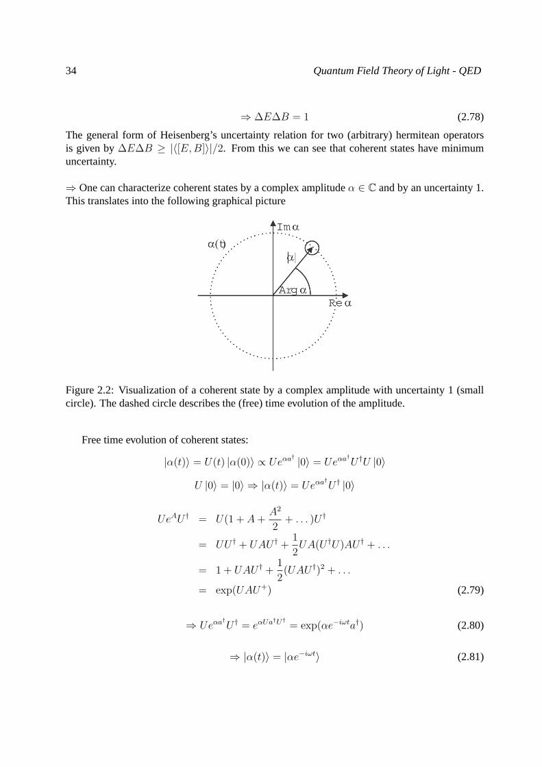
⇒ One can characterize coherent states by a complex amplitudeα ∈ C and by an uncertainty 1.This translates into the following graphical picture
Figure 2.2: Visualization of a coherent state by a complex amplitude with uncertainty 1 (smallcircle). The dashed circle describes the (free) time evolution of the amplitude.
Free time evolution of coherent states:
|α(t)〉 = U(t) |α(0)〉 ∝ Ueαa† |0〉 = Ueαa
†U †U |0〉
U |0〉 = |0〉 ⇒ |α(t)〉 = Ueαa†U † |0〉
UeAU † = U(1 + A+A2
2+ . . . )U †
= UU † + UAU † +1
2UA(U †U)AU † + . . .
= 1 + UAU † +1
2(UAU †)2 + . . .
= exp(UAU+) (2.79)
⇒ Ueαa†U † = eαUa
†U†= exp(αe−iωta†) (2.80)
⇒ |α(t)〉 = |αe−iωt〉 (2.81)
2.3 Classical and Quantum Mechanical Interference 35
Hence, coherent states remain coherent states and their amplitude moves on a circle around theorigin of the complex plane.
• Coherent states arenot orthogonalto each other:
〈α|β〉 = e−|α|2
2 e−|β|2
2 eα∗β (2.82)
The proof can be done using the expansion in number states or the displacement operatorand Baker-Campbell-Hausdorf equation (Eq. (2.69) on page 32).
• Coherent states areovercomplete: ∫d2α |α〉 〈α| = π1 (2.83)
Proof: Expansion in number states and integration over the phase angle ofα.
2.3 Classical and Quantum Mechanical Interference
The difference between classical and quantum mechanical interference is at first sight rathersubtle, but can be well understood using coherent states. Set|ψ〉 = |α〉 = D(α) |0〉; D†(α) =D−1(α).
D(α) can be used to switch to a unitarily equivalent”picture“ in which the state|ψ〉 =
D−1(α) |ψ〉 coincides with the vacuum. The operators then transform as
ˆO = D†(α)OD(α) (2.84)
(⇐⇒ 〈ψ| ˆO|ψ〉 = 〈ψ|O|ψ〉)
E(x) = D†(α)E(x)D(α)
=∑akσ 6=a
(akσ . . . eikx + H.c.) + i
√~ωa
2(2π)3ε0εae
ikxD†(α)aD(α) + H.c.
=
∫dk∑σ
akσ . . .+ H.c.+ i√. . .εae
ikxD†aD + H.c.
To calculateD†(α)aD(α) we use the theorem
eABe−A =∞∑n=0
1
n!kn k0 = B; kn+1 = [A, kn] (2.85)
36 Quantum Field Theory of Light - QED
=⇒ A = α∗a− αa†;B = a
=⇒ k0 = a; k1 =[α∗a− αa†, a
]= α
=⇒ k2 = k3 = . . . = 0
=⇒ D†(α)aD(α) = a+ α
E(x) = EAll other modes+ (i√. . .εae
ikxa− i√. . .ε∗ae
−ikxa†)
+(iα√. . .εae
ikx − i√. . .ε∗aα
∗e−ikx)
=⇒ E(x) = E(x) + Eclassicala (x) (2.86)
The state|α〉 in absence of external classical fields is thus unitarily equivalent to thevacuum in the presence of the fieldEclass.
a (x) (andBclass.a (x)).
We can exploit this equivalence to understand the difference between the interference of photonsand classical Maxwell fields:
• Classical interference:
E = E1 + E2, e.g.Ei ∝ eikix
I ∝ EE∗ = |E1|2 + |E2|2 + 2Re(E1E∗2)
2Re(E1E∗2) ∝ cos(x(k1 − k2))
• Quantum description of classical interference:
|ψ〉 = |α1, α2〉= D1(α1)D2(α2) |0〉
D1(α1) = eα1a†1−α∗1a1
D2(a2) analogously
The product of operatorsD1D2 creates the sum of classical fields,
D†2D†1ED1D2 = D†2(E + E1)D2 = E + E1 + E2
Transformation usingD†2D†1 from |ψ〉 to the vacuum:
I ∝ 〈ψ|E(−)E(+)|ψ〉 = 〈0|(E(−)
+ E∗1 + E∗2)(E(+)
+ E1 + E2)|0〉= |E1 + E2|2
⇐⇒ classical interference fringes
2.4 Remarks on the Quantization Procedure for other Gauges 37
In quantum mechanics one can also consider superpositions of coherent states. This does notdescribe classical fields anymore:
|ψ〉 = |α1〉+ |α2〉 = (D1(α1) +D2(α2)) |0〉
Interference fringes for this state:
I ∝ 〈ψ|E(−)
E(+)|ψ〉
= 〈0|(D†1 +D†2)E(−)
E(+)
(D1 +D2)|0〉= 〈0|(D†1E(−)E(+)D1 +D†1E
(−)E(+)D2 +D†2E(−)E(+)D1 +D†2E
(−)E(+)D2)|0〉= |E1|2 + |E2|2 + 〈0|(D†1E(−)E(+)D2 +D†2E
(−)E(+)D1)|0〉= |E1|2 + |E2|2 + 〈α1|E(−)E(+)|α2〉+ 〈α2|E(−)E(+)|α1〉
=⇒ I ∝ |E1|2 + |E2|2 + E∗1E2 〈α1|α2〉+ E∗2E1 〈α2|α1〉
〈α1|α2〉 = e−|α1|
2
2 e−|α2|
2
2 eα∗1α2
=⇒ | 〈α1|α2〉 |2 = . . . = e−|α1−α2|2
=⇒ For |α1 − α2| 1 quantum interference is strongly suppressed. For a classical field witha large number of photons|α|2 1 it is therefore unimportant. The state|α1〉 + |α2〉 is alsocalled Schrodinger cat state since it corresponds to a superposition of macroscopic states (for|αi|2 1).
2.4 Remarks on the Quantization Procedure for other Gauges
The fact that we have only quantizedA but notφ is connected to our choice of Coulomb gauge.Reason:A = 0 ∆φ = 0=⇒ φ is not dynamical, the corresponding conjugate momentum vanishes. This can be under-stood with the aid of the Lagrangean:
L =1
2
∫(E2 − c2B2)d3x
=1
2
∫[(−∇φ− A)2 − c2(rotA)2]d3x
=1
2
∫[(∇φ)2 + 2φdivA + A
2 − c2(rotA2)]d3x
=
∫Ld3x
Coulomb gauge:
divA = 0 =⇒ ∂L∂φ
= 0
38 Quantum Field Theory of Light - QED
Lorentz gauge:
divA +1
c2φ = 0 =⇒ L =
1
2
∫[(∇φ)2 − 2φφ
1
c2+ A
2 − c2(rotA2)]d3x
If one now considers the actionS =∫Ldt one can integrate by part the term∝ φ and arrives at
a new Lagrangean densityL′ ∝ φ2. One therefore gets∂L′/∂φ 6= 0 so that the scalar canonicalmomentum is nonzero.
=⇒ in Lorentz gauge we do not only have to circularly polarized photons but also a scalarphoton(⇐⇒ φ) and a longitudinally polarized one(⇐⇒ divA 6= 0). The two new photons are
unphysical and have to be removed by imposing appropriate constraints:(divA+˙φ/c2) |ψ〉 !
= 0)for physical states|ψ〉.
A unified prescription to quantize constrained systems has been developed (among others)by Dirac, but it is rather sophisticated (see, for instance, chapter 1 of Ref. [10]).
Chapter 3
Quantum Mechanics of Atoms: a shortReview
3.1 The Hydrogen Atom, Parity
Hamilton operator for a proton and an electron (V= Coulomb potential):
H =p2p
2Mp
+p2e
2me
+ V (|xp − xe|) (3.1)
R = 1Mp+me
(Mpxp+mexe) is the center-of-mass coordinate,r = xe−xp the relative coordinate
between the two particles,M = Mp+me, 1µ
= 1Mp
+ 1me
. The Hamiltonian then can be rewrittenas
H =P 2
2M+
p2
2µ+ V (|r|) (3.2)
In traditional atomic and molecular physics the relative motion is the central topic, in atomoptics the center-of-mass motion.
Introducespherical coordinatesfor the relative motion:
=⇒ p2
2µ= − ~2
2µ·
(1
r∂rr∂r −
L2
r2
)(3.3)
with p = −i~∇ and L being the orbital angular momentum. One finds[L, |r|] = 0. Theeigenstates ofH are therefore also eigenstates ofL:
ψ = Ylm(θ, φ)fl(r)
L2Ylm = ~2l(l + 1)Ylm(3.4)
The radial partfl(r) of the wavefunction fullfills
Efl =
(− ~2
2µ
1
r∂rr∂r +
~2
2µ
l(l + 1)
r2+ V (r)
)fl (3.5)
40 Quantum Mechanics of Atoms: a short Review
Solution: fnl ∼ rl exp(− rna0
)· Laguerre polynomials,a0 = Bohr radius≈ 0, 5 A.
=⇒ Ψnlm = fnlYlm(θ, φ) ⇐⇒ |nlm〉 (electronicstate) (3.6)
Heren denotes the principal quantum number,l the orbital abgular momentum, andm themagnetic quantum number. There is one additional quantum number:Spins of the electron,s = ±1
2, |ψ〉 = |nlms〉 .
Parity:
r −→ −r
|r| −→ |r|Ylm(θ, φ) −→ Ylm(π − θ, φ+ π) = (−1)lYlm(θ, φ)
(3.7)
=⇒ The parity of|nlms〉 is (−1)l. Parity is very important for the dipole selection rules ofatomic radiation.
3.2 Fine structure and spin
Of high practical relevance is the interaction of an atom with a static magnetic field,
H = −µ ·B (3.8)
whereµ is the magnetic dipole moment of the atom. A classical particle with angular momentumL (e.g., on a circular orbit) and chargeq possesses the magnetic moment
µ =q
2ML. (3.9)
The orbital contribution of the electron is
µe = − e
2me
L . (3.10)
For the proton we have because ofMp me
µp = +e
2Mp
L µe . (3.11)
Spin of the electron:1
− e
2me
2S = − ~e2me
σ. (3.12)
1The factor of 2, which appears here in contrast to the orbital angular momentum, is called gyromagnetic factorg. It follws from Dirac’s equation for a relativistic electron thatg = 2. However, vacuum fluctuations of theelectromagnetic field cause small deviations from this value (g ≈ 2, 002).
3.3 Hyperfine structure 41
is a consequence of the magnetic field which is created in the rest frame of the electronbecause of its motion around the nucleus. In the electrons rest frame the nucleus represents amoving charged particle, corresponding to an electric current that induces a magnetic field.
Rest frame of the nucleus: electric fieldE = −∇VCoul, B = 0 (the nucleus creates nomagnetic field as it is not moving in this frame).
Lorentz transformation to the electron’s rest frame2:
B′ = v ×E
= −v ×∇VCoul
= − 1
Mp×∇VCoul
(3.13)
wherev is the velocity.
VCoul = VCoul(|r|) =⇒ ∇VCoul = er∂rVcoul = r1
r∂rVCoul
=⇒ B′ = − 1
M
(1
r∂rVCoul
)p× r =
1
M
(1
r∂rVCoul
)L(e−)
(3.14)
Thus, there exists a coupling between spin and orbital angular momentum of the electron:
HSB = −µeσB′
= µeσ ·L(
1
r∂rVCoul
)(3.15)
An exact calculation of the matrix elements〈n′l′m′s′|HSB|nlms〉, including relativistic cor-rections, leads to
∆EFS = −1
2mec
2(αZ)4 1
h3
(1
j + 12
− 3
4n
)∆EFS/~ ≈ 100GHz
(3.16)
wherej = l ± 12
denotes the total angular momentum of the electron.Without relativistic corrections∆EFS would depend onl ands instead onj = l + s.
3.3 Hyperfine structure
Hyperfine structure is caused by two different effects:
1. Interaction between the electron’s angular momentum and the nuclear spin.
2Actually the electron is moving on a non-inertial (circular) orbit and it is necessary to proceed differently.However, the result presented here agrees with the correct one up to a factor of 1/2 (Thomas factor) and explains therelevant physical ideas.
42 Quantum Mechanics of Atoms: a short Review
2. QED corrections (vacuum fluctuations)
ad 1.: A magnetic dipole moment xreates a magnetic field which other magnetic momenta caninteract with. For the hydrogen atom the total angular momentumj = s + l of the electroncreates a magnetic field at the position of the nucleus with which the latter’s spin interacts.
Hyperfine spin:F = Sk + j (3.17)
Is has to be remarked that the addition ofSk andj to F is not fully equivalentto the addition ofthe total spinSG = Sk +Se and the electronic orbital angular momentumL to F . This happensalthough the operators themselves are exactly equal. The reason is that with each of the twoadditions one associates a certain set of basis vectors diagonalizingF . The two bases associatedwith F = Sk + j andF = SG + L are different, see Appendix 12.2.
Chapter 4
The Interaction between Atoms and Light
4.1 Minimal Coupling
The classical Maxwell equations are gauge invariant,
A → A′ = A +∇χ , φ→ φ′ = φ− ∂tχ . (4.1)
This invariance holds also in the presence of charge densities% and currentsj and should also bepresent in the quantum description of electromagnetic fields.
4.1.1 Derivation of Minimal Coupling
The equation of motion for charged particles,
mx = qE + qx×B electric + Lorentz force
can be derived from the Lagrangean ,
L =1
2mx2 + qxA(x, t)− qφ(x, t) , (4.2)
in the following way. Thecanonically conjugated momentump is defined by
pi :=∂L
∂xi⇒ pi = mxi + qAi(x, t) (4.3)
Therefore, in the presence of an electromahnetic field the canonically conjugated momentum isdifferent from thekinetic momentumΠ = mx. The Euler-Lagrange equations are given by
d
dtpi =
∂L
∂xi(4.4)
44 The Interaction between Atoms and Light
Insert (4.2) and (4.3):
∂L
∂xi= −q∂iφ+ qxk∂iAk
d
dtpi = mxi + q
∂
∂tAi (x(t), t) + q
∂
∂xkAi (x(t), t) xk
=⇒ mxi = −q∂iφ− q∂tAi + qxk(∂iAk − ∂kAi) (4.5)
verwenden−∂iφ− ∂tAi = Ei (by definition)
=⇒ mxi = qEi + qxk(∂iAk − ∂kAi) (4.6)
However,Bj = (rotA)j = εjmn∂mAn
=⇒ εikjBj = εikjεjmn∂mAn
= εjikεjmn∂mAn
= (δimδkn − δinδkm)∂mAn
= ∂iAk − ∂kAi (4.7)
=⇒ mxi = qEi + qxkεikjBj
= qEi + q(x×B)i qed.
Using the Lagrange function one can derive the Hamiltonian and Schrodinger’s equation:The classical Hamiltonian is defined by
H = pixi − L
Usingx = 1m
(p− qA) we want to write it as a function ofp andx =⇒
H = pi1
m(pi − qAi)−
1
2m
1
m2(p− qA)2 − q
1
m(p− qA)A + qφ
H =1
2m(p− qA)2 + qφ
The corresponding quantum mechanical Hamiltonian can be found by canonical quantisation:
x → x ; p → p ; [xi, pj] = δij
In position representation:x → x ; p → −i~∇
and therefore
H =1
2m(−i~∇− qA(x, t))2 + qφ(x, t) , i~∂tψ(x, t) = Hψ(x, t) (4.8)
This is the Schrodinger equation for a non-relativistic particle in an electromagnetic field. Theform (p− qA) is calledminimal coupling.
4.1 Minimal Coupling 45
4.1.2 Gauge Invariance of Minimal Coupling
Applying the transformation (4.1) to the Hamiltonian (4.8) one could be led to the conclusionthat the Schrodinger equation is not gauge invariant:
H ′ =1
2m(−i~∇− qA(x, t)− q∇χ)2 + qφ(x, t)− q
∂χ
∂tψ
i~∂tψ(x, t) 6= Hψ(x, t)
To restore the invariance under gauge transformations one also has to unitarily transform thewavefunction:
ψ′ = ψ exp(iqχ/~) (4.9)
This implies
i~∂tψ′ = eiqχ/~i~∂ψ
∂t− q
∂χ
∂tψ
= eiqχ/~
Hψ − q
∂χ
∂tψ
= eiqχ/~
1
2m(−i~∇− qA)2 + qφ
ψ − q
∂χ
∂tψ′
=
1
2m(−i~∇− qA− q∇χ)2 + qφ
(eiqχ/~ψ
)− q
∂χ
∂tψ′
= H ′ψ′ (4.10)
The minimal coupling scheme is of outstanding importance for high energy physics. Apartfrom gravity, all fundamental forces (that is, electromagnetic, weak, and strong interaction) dohave the same basic structure. The simplest form of a gauge invariant theory is realized for theelectromagnetic field. It is also called U(1) gauge theory because the transformation of the state(4.9) corresponds to a multiplication with aUnitary1×1 matrix (= complex number of modulus1). The other fundamental forces couple more fields. For example, theSpecialunitary SU(2)gauge theory of (electro-)weak interaction transforms the fields according to(
ψ′eψ′νe
)= exp(iσ · χ)
(ψeψνe
)(4.11)
Hereψe is the wavefunction of the electron,ψνe that of the electron-neutrino, andσ are thePauli matrices. The wordspecialimplies that the matrixexp(iσ · χ) has determinant 1. Thegauge potential for this theory can be written asA = A(i)σi and therefore conists of Threevector fieldsA(i). These three fields do roughly correspond to the W± and the Z Boson whichmediate the weak interaction between different particles, in the same way as photons do for theelectromagnetic force.1
1Actually the weak and the electromagnetic forces are entangled. Both together are described by a U(1)×SU(2)gauge theory. U(1) thereby refers to hypercharge and not to the electromagnetic charge.
46 The Interaction between Atoms and Light
4.2 The Power-Zienau-Woolley Transformation
Although minimal coupling is of highest importance for the description of the fundamentalforces, it has several disadvantages when one wants to describe the interaction between atomsand light:
• For electrically neutral atoms which are composed of electrons, neutrons, and protons,minimal coupling is somewhat inconvenient. It would be better to describe the interactionusing the atomic multipole moments.
• In minimal coupling the gauge potentials instead of the electric and magnetic field describethe coupling. Although this is not a principal problem a direct coupling to the physicalfields would be manifestly gauge invariant and more intuitive.
• In Coulomb gauge the scalar potentialφ can be identified with the unretarded Coulombpotential, since the latter solves Poisson’s equation (which the equation forφ). The factthat the Coulomb potential is unretarded makes it appear as if minimal coupling wouldproduce an instantaneous long-range force between the atoms.
The Power-Zienau-Woolley transformation (Refs. [28] and [29], see also [30] and [31]) isa unitary transformation of the minimal coupling. It leads to an equaivalent description of theinteraction, but with the above problems removed.
4.2.1 The Basic Idea
To derive the so-called dipole coupling2 one can start from the fact that the Euler-Lagrangeequations are not changed when one adds a total time derivative to the Lagrnangean,
L′(x, x, t) = L(x, x, t) +d
dtF (x, t) =⇒ d
dt
∂L′
∂x− ∂L′
∂x=
d
dt
∂L
∂x− ∂L
∂x
For simplicity we consider here only constant fieldsE andB (for the general proof see below).
E = E0; B = B0 ⇐⇒ φ = −xE0
A = −1
2(x×B0)
2A more precise name which is also used in the literature ismultipolar couplingsince the full Power-Zienau-Woolley transformation leads to a coupling of the electromagnetic field to all multipole moments of the atoms.However, in the applications one very often only takes the dipole moment into account. This is also the case for thesimple example in this subsection.
4.2 The Power-Zienau-Woolley Transformation 47
ChoosingF = −qxA one arrives at
d
dtF = −qxA +
q
2(x× x)B0 (4.12)
L′ =1
2mx2 + qxA + qxE0︸ ︷︷ ︸
L
−qxA +q
2(x× x)B0 (4.13)
=1
2mx2 + qxE0 +
q
2mLB0 mit L = (x×mx) (4.14)
Setting d := qx electric dipole moment of the particleµ := q
2mL magnetic moment of the particle
one finds for the new Lagrangean
L′ =1
2mx2 + dE0 + µB0
Advantage: Now the canonical momentum agrees with the kinetic momentum,p = mx. In ad-dition, the particle now couples to the physical fields and therefore is manifestly gauge invariant.It also involves the dipole momenta which are better suited for electrically neutral particles.
4.2.2 The Complete Transformation
We consider an ensemble of point particles with chargesqα and positionsxα. Their chargedensity is given by
%(x) =∑α
qαδ(x− xα) (4.15)
Since we are particularly interested in the behaviour of a gas of neutral atoms, we assume thatthe total charge is zero,
∑α qα = 0. The polarization of macroscopic Electrodynamics fullfills
divP = −〈%geb〉 (see Sec.??). For the present case its solution is given by
P (x) =∑α
∫ 1
0
du qα(xα −R)δ(x−R− u(xα −R)) (4.16)
Proof:
∂iP i(x) =∑α
∫ 1
0
du qα(xα −R)i∂iδ(x−R− u(xα −R))
=∑α
∫ 1
0
du qα(xα −R)iδ′(xi −Ri − u(xα −R)i)×
δ(xj −Rj − u(xα −R)j)δ(xk −Rk − u(xα −R)k) , (4.17)
where we sum overi and (i, j, k) = (1, 2, 3), (2, 3, 1), (3, 1, 2). δ′ is the derivative of theδ-distribution. We have
(xα −R)iδ′(xi −Ri − u(xα −R)i) = −∂uδ(xi −Ri − u(xα −R)i) (4.18)
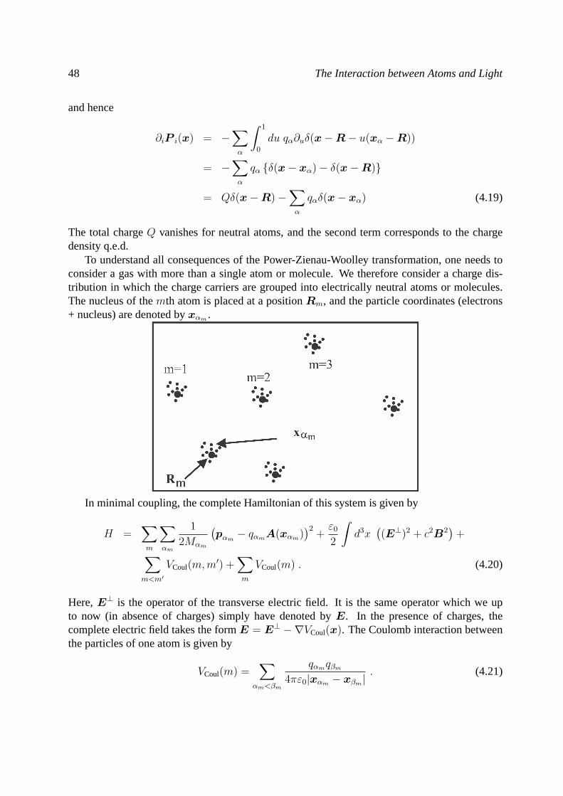
48 The Interaction between Atoms and Light
and hence
∂iP i(x) = −∑α
∫ 1
0
du qα∂uδ(x−R− u(xα −R))
= −∑α
qα δ(x− xα)− δ(x−R)
= Qδ(x−R)−∑α
qαδ(x− xα) (4.19)
The total chargeQ vanishes for neutral atoms, and the second term corresponds to the chargedensity q.e.d.
To understand all consequences of the Power-Zienau-Woolley transformation, one needs toconsider a gas with more than a single atom or molecule. We therefore consider a charge dis-tribution in which the charge carriers are grouped into electrically neutral atoms or molecules.The nucleus of themth atom is placed at a positionRm, and the particle coordinates (electrons+ nucleus) are denoted byxαm.
In minimal coupling, the complete Hamiltonian of this system is given by
H =∑m
∑αm
1
2Mαm
(pαm
− qαmA(xαm))2
+ε0
2
∫d3x
((E⊥)2 + c2B2
)+∑
m<m′
VCoul(m,m′) +
∑m
VCoul(m) . (4.20)
Here,E⊥ is the operator of the transverse electric field. It is the same operator which we upto now (in absence of charges) simply have denoted byE. In the presence of charges, thecomplete electric field takes the formE = E⊥ −∇VCoul(x). The Coulomb interaction betweenthe particles of one atom is given by
VCoul(m) =∑
αm<βm
qαmqβm
4πε0|xαm − xβm|. (4.21)
4.2 The Power-Zienau-Woolley Transformation 49
On the other hand, the interaction between the particles of two different atoms can be written as
VCoul(m,m′) =
∑αm,βm′
qαmqβm′
4πε0|xαm − xβm′ |. (4.22)
To construct the unitary transformation that connects minimal coupling to multipolar cou-pling, we employ the total polarization of the gas, which is a sum over the polariztion of theindividual atoms:
P (x) =∑m
Pm(x) (4.23)
Pm(x) =∑αm
∫ 1
0
du qαm(xαm −Rm) δ(x−Rm − u(xαm −Rm)) . (4.24)
ThePower-Zienau-Woolley-Transformationis then given by
U = exp
(i
~
∫d3x P (x) ·A(x)
)(4.25)
Explicit expressions for the transformation
Our task is to find explicit expressions for the transformed Hamiltonian and other operators ofrelevance. SinceU is a function ofxαm andA(x), it is obvious that because[Ai(x),Aj(x
′)] =[Ai(x),Bj(x
′)] = 0 the vector potential, the magnetic field and the particle coordinates as wellas the polarization transform trivially,
A = U †AU = A (4.26)
B = B (4.27)
xαm = xαm (4.28)
P = P . (4.29)
All other fields can be treated by using the theoremexp(−iS)E exp(iS) = E − i[S,E] + · · · .We find for the electric field
E⊥i (x) = E⊥i (x)− i
~
∫d3x′ P j(x
′)[Aj(x′),E⊥i (x)] (4.30)
= E⊥i (x)− i
~
∫d3x′ P j(x
′)−i~ε0
δ⊥ij(x− x′) . (4.31)
Recalling that the transverse (source-free) part of a vector fieldP is given by(TP )i(x) =∫d3x′ P j(x
′)δ⊥ij(x− x′), we can derive
E⊥(x) = E⊥(x)− 1
ε0
P⊥(x) . (4.32)
50 The Interaction between Atoms and Light
This equation has some interesting consequences. If we write it in the form
ε0E⊥(x) = ε0E
⊥(x) + P
⊥(x) = D
⊥(4.33)
it becomes obvious that theoldoperatorε0E⊥ of the electric fieldin the new pictureplays the role
of the dielectric displacement fieldD⊥
. In other words: if one uses minimal coupling, the electricfield is given byE⊥ and the dielectric displacement byε0E
⊥ + P⊥. In dipole coupling, the
electric field is given byE⊥
and the dielectric displacement byε0E⊥
+ P⊥
= ε0E⊥. Since the
operatorE⊥ has a simple form, it is also used in multipolar coupling to express the interaction.it remains to calculate the transformation of the particle momenta. One easily finds
pαm= pαm
− i[S,pαm] + · · ·
= pαm+ ~∇αmS . (4.34)
The calculation of the gradient will be done below. In summary we obtain for the transformedHamiltonian the expression
H =∑m
∑αm
1
2Mαm
(pαm
+ ~∇αmS − qαmA(xαm))2
+ε0
2
∫d3x
(1
ε20
(D⊥ − P⊥)2 + c2B2
)+∑
m<m′
VCoul(m,m′) +
∑m
VCoul(m) (4.35)
Calculation of the polarization integrals
This expression can be considerably simplified. We start with the second line:
1
2ε0
∫d3x (D
⊥ − P⊥)2 =1
2ε0
∫d3x
((D⊥)2 − 2D
⊥ · P⊥ + (P⊥)2)
(4.36)
=1
2ε0
∫d3x
((D⊥)2 − 2D
⊥ · P⊥ + (P − P ‖)2),
whereP ‖ denotes the longitudinal part of the vector field (i.e., the Fourier transform of the fieldis parallel to the wave vector, not transverse). We can now make use of the following relation,∫
d3x R⊥(x) · S(x) =
∫d3x R⊥(x) · S⊥(x) . (4.37)
To prove it we first show that the transversalization operator is idempotent. By definition, wehave
(T 2R)i(x) =
∫d3x′δ⊥ij(x− x′)
∫d3x′′δ⊥jk(x
′ − x′′)Rk(x′′) . (4.38)
4.2 The Power-Zienau-Woolley Transformation 51
With∫d3x′δ⊥ij(x− x′)δ⊥jk(x
′ − x′′) =
∫d3x′
∫d3k
(2π)3
d3k′
(2π)3eik·(x−x′)eik
′·(x′−x′′) ×(δij −
kikj
k2
)(δjk −
k′jk′k
(k′)2
)=
∫d3k
(2π)3eik·(x−x′′)
(δij −
kikj
k2
)(δjk −
kjkk
k2
)= δ⊥ik(x− x′′) (4.39)
it follows that
(T 2R)i(x) =
∫d3x′′δ⊥ik(x− x′′)Rk(x
′′)
= (TR)i(x) (4.40)
In addition,T is Hermitean with respect to the standard scalar product:∫d3x R(x) · (TS)(x) =
∫d3x Ri(x)
∫d3x′δ⊥ij(x− x′)Sj(x
′)
=
∫d3x′(TR)(x′) · S(x′) (4.41)
Relation (4.37) then follows from∫d3x R⊥(x) · S(x) =
∫d3x (TR)(x) · S(x)
=
∫d3x (T 2R)(x) · S(x)
=
∫d3x (TR)(x) · (TS)(x)
=
∫d3x R⊥(x) · S⊥(x) . (4.42)
Eq. (4.37) is helpful to simplify the integral over the polarization:
1
2ε0
∫d3x
(P 2 − 2P · P ‖ + (P ‖)2
)=
1
2ε0
∫d3x
(P 2 − 2(P ‖)2 + (P ‖)2
)=
1
2ε0
∫d3x
(P 2 − (P ‖)2
)(4.43)
The integration over the longitudinal part can be calculated exactly. Since the source of this termis the charge distribution, divP = divP ‖ = −%, it is reasonable that it is related to the Coulomb
52 The Interaction between Atoms and Light
potential. To demonstrate this we first rewrite the latter in the form
VCoul(x) =1
4πε0
∫d3x′
%(x′)
|x− x′|
=−1
4πε0
∫d3x′
divP ‖(x′)
|x− x′|
=1
4πε0
∫d3x′ P
‖i (x
′)∂′i1
|x− x′|(4.44)
The gradient of the Coulomb potential, which simply is the negative longitudinal electric field,we find
∂jVCoul(x) =1
4πε0
∫d3x′ P
‖i (x
′)∂j∂′i
1
|x− x′|
=−1
4πε0
∫d3x′ P
‖i (x
′)∂j∂i1
|x− x′|(4.45)
To calculate the double derivative of the integrand, we use the Fourier transform∫d3x
e−ik·x
|x|=
4π
k2 (4.46)
To prove this one can use spherical coordinates, with the z-axis alongk. One then finds3∫d3x
e−ik·x
|x|=
∫ ∞0
r2dr d cosϑ dϕe−ikr cosϑ
r
= 2π
∫ ∞0
rdr1
−ikr(e−ikr − eikr)
=2πi
k
πδ(k)− i
Pk−(πδ(k) + i
Pk
)=
4π
k2 (4.47)
We thus find for the double derivative
∂j∂i1
|x− x′|= ∂j∂i
∫d3k
(2π)3
4πeik·(x−x′)
k2
= −4π
∫d3k
(2π)3eik·(x−x′)kikj
k2
= −4π(δijδ(x− x′)− δ⊥ij(x− x′)
)(4.48)
3The omission of the principal partP in the last line is based on the following considerations. Like everydistribution,P/k is only defined as an integrand and needs to be multiplied with a test function (which has to beinfinitely often differentiable, normalizable, without poles). In the second-to-last row, an additional factor of1/kappears, which is not a test function. Therefore, the result is only properly defined if one considers test functionswhich go at least linearly against zero fork → 0. In theoretical physics, however, it is customary to use this equationwithout caring about test functions. The principal value is then meaningless, since it does not result in a finite valueif the divergence is of the form1/k2. It is therefore simply omitted.
4.2 The Power-Zienau-Woolley Transformation 53
so that
∂jVCoul(x) =−1
4πε0
∫d3x′ P
‖i (x
′)(−4π)(δijδ(x− x′)− δ⊥ij(x− x′)
)=
1
ε0
P‖j(x) (4.49)
The longitudinal electric field is therefore completely characterized by the polarization, so that
− 1
2ε0
∫d3x (P ‖)2 = −ε0
2
∫d3x (∇VCoul)
2
=ε0
2
∫d3x VCoul∆VCoul
= −1
2
∫d3x VCoul% , (4.50)
where the last line follows from the Coulomb potential obeying Poisson’s equation. InsertingEq. (4.15) for the charge density, one arrives at
− 1
2ε0
∫d3x (P ‖)2 = −1
2
∑m,αm
∑m′,α′
m′
qαmqα′m′
4πε0|xαm − xα′m′ |
(4.51)
In this expression, we have to remove the terms with indentical particles since they diverge. Therest is symmetric under exchange of primed and unprimed indices, so that
− 1
2ε0
∫d3x (P ‖)2 = −
∑m<m′
∑αm,α′m′
qαmqα′m′
4πε0|xαm − xα′m′ |
−∑m
∑αm<α′m
qαmqα′m4πε0|xαm − xα′m|
= −∑m<m′
V (m,m′)−∑m
V (m) (4.52)
The integral over the longitudinal part of the polarization therefore exactly cancels the Coulombinteraction between the atoms. This is the reason why we decomposed the polarization into thecomplete and the longitudinal polarization in Eq. (4.36). The remaining integral over the com-plete polarization field can now be decomposed into the individual contribution of each atom,∫
d3x P 2 =∑m,m′
∫d3x PmPm′ (4.53)
In Eq. (4.24) one can see that the polarization of themth atom is strongly localized around theatom itself. Since in an atomic gas the distance between the atoms is much larger then their size,
54 The Interaction between Atoms and Light
one can neglect terms withm 6= m′ and thus deduces
1
2ε0
∫d3x P 2 ≈ 1
2ε0
∑m
∫d3x P 2
m
=1
2ε0
∑m
∫d3x
((P⊥m)2 + (P ‖m)2
)=
1
2ε0
∑m
∫d3x (P⊥m)2 +
∑m
V (m) (4.54)
Hamiltonian and multipolar expansion
Inserting all calculations in the transformed Hamiltonian (4.35) one obtains
H =∑m
Hm +Hrad +Hint (4.55)
Hm =∑αm
p2αm
2Mαm
+ V (m) +1
2ε0
∫d3x (P⊥m)2 (4.56)
Hrad =1
2ε0
∫d3x (D⊥)2 +
1
2µ0
∫d3x B2 (4.57)
Hint = − 1
ε0
∫d3x D⊥ · P
+∑m,αm
1
2Mαm
(nαm · pαm
+ pαm· nαm + (nαm)2
)(4.58)
with
(nαm)i := ~(∇αm)iS − qαmAi(xαm) (4.59)
= ~(∇αm)i
∫ 1
0
du qαm(xαm −Rm) ·A(Rm + u(xαm −Rm))− qαmAi(xαm)
=
∫ 1
0
du qαm
(Ai(Rm + u(xαm −Rm))
+(xαm −Rm)ju∂iAj(Rm + u(xαm −Rm)))− qαmAi(xαm)
The vectornαm can be brought into a form which is explicitly independent from the potential.To do so one uses∫ 1
0
du u∂uA(Rm + u(xαm −Rm)) = A(xαm)−∫ 1
0
du A(Rm + u(xαm −Rm)) (4.60)
4.3 Dipole approximation and dipole coupling 55
which can be proven by partial integration. Introducing the notationrαm := xαm−Rm it followsthat
(nαm)i :=
∫ 1
0
du qαm (Ai(Rm + urαm) + (rαm)ju∂iAj(Rm + urαm))
−∫ 1
0
du qαm (u∂uAi(Rm + urαm) + Ai(Rm + urαm))
=
∫ 1
0
du qαm ((rαm)ju∂iAj(Rm + urαm)− u(rαm)j∂jAi(Rm + urαm))
=
∫ 1
0
du qαmu(rαm)j (∂iAj(Rm + urαm)− ∂jAi(Rm + urαm)) (4.61)
and therefore, because of∂iAj − ∂jAi = εijkBk,
nαm = qαm
∫ 1
0
u du (xαm −Rm)×B(Rm + u(xαm −Rm)) (4.62)
This is the final form of the multipolar Hamiltonian. We emphasize again that no approx-imation has been made aprt from the assumption that the total polarizations of two differentmolecules have little overlap. It is therefore fully justified to use this coupling instead of mini-mal coupling. The most important features of the Hamiltonian (4.55) are as follows.
• It is explicitly gauge invariant since it only contains the electric and the magnetic field.
• The Coulomb potential between different atoms has disappeared. The interaction between
the atoms is now exclusively mediated through the retarded dynamical fieldsD⊥
andB.
4.3 Dipole approximation and dipole coupling
The typical sizer of an atom is in the order of Bohr’s radius (≈ 0.5 × 10⁻¹⁰ m). Since opticalwavelengthsλ = 2π/k are in the range of several hundreds of nm, it is justified to restrict themultipolar expansion of the interaction Hamiltonian after the first few terms. The reason is thatmultipole moments of orderl are proportional to(kr)l andkr 1 is valid, see Eq. (1.15). We
56 The Interaction between Atoms and Light
therefore keep only the lowest order terms and obtain for the polarization
P (x) =∑m
Pm(x)
=∑m
∑αm
qαm(xαm −Rm)
∫ 1
0
du δ(x−Rm − u(xαm −Rm))
≈∑m
∑αm
qαm(xαm −Rm)
∫ 1
0
du δ(x−Rm) +O(|xαm −Rm)|2)
=∑m
δ(x−Rm)∑αm
qαm(xαm −Rm)
=∑m
δ(x−Rm)dm , (4.63)
wheredm is the dipole moment of themth atom/molecule. Analogously one finds for the secondcoupling term
nαm ≈ qαm
∫ 1
0
u du (xαm −Rm)×B(Rm) +O(|xαm −Rm)|2) (4.64)
and thus
nαm · pαm+ pαm
· nαm + (nαm)2 ≈ 2qαmpαm·∫ 1
0
u du (xαm −Rm)×B(Rm)
= −qαmLαm ·B(Rm) (4.65)
This is thedipole approximation. The associated interaction Hamiltonian is calleddipole cou-pling and given by
Hint = − 1
ε0
∑m
dm · D⊥(Rm)−
∑m
µm ·B(Rm) (4.66)
whereµm =∑
αmqαmLαm/(2Mαm) is the magnetic dipole moment that is associated with the
orbital angular momentum of the electrons. The spin contribution simply doesn’t appear herebecause it is omitted in our treatment of the Power-Zienau-Woolley transformation. It would ofcourse be present if we start from particles with spin.
We remark that only the complete multipolar Hamiltonian is unitarily equivalent to the min-imal coupling scheme. As soon as approximations are made, the use of the different interactionforms leads to slightly different results. We will consider an example for this in the next chapter.In quantum optics, using dipole coupling usually results in slightly better results.
4.4 Selection rules for atoms
One of the most important questions in atomic physics and quantum optics is which levels arecoupled by a given electromagnetic field. To examine this we consider a single atom whose
4.4 Selection rules for atoms 57
nucleus rests at the origin (Rm = 0, it is a very good approximation to neglect the center-of-mass motion in the derivation of selection rules). Since all the other particles are electrons, theelectric dipole moment can be written as
dm =∑αm
qαm(xαm −Rm)
= −e∑αm
xαm
=: −er (4.67)
r is the sum over the position of the electrons relative to the nucleus. in the following we willomit the indexm, since we consider a single atom only,dm → d, αm → α etc. Here, the sumincludes only the electrons. If there are any contributions from the nucleus, they will be addedexplicitly.
We have seen in chapter 3 that atomic states are, to a very good approximation, eigenstatesof the total angular momentum
F = sK +∑α
(Lα + sα) , (4.68)
with the atomic state|ψ〉 = |F,mF , · · · 〉. Since the interaction is mediated through the dipolemoment, the transition amplitudes between|F,mF 〉 and|F ′,m′F 〉 are proprtional to
dF,mF ;F ′,m′F
:= 〈F,mF | − er|F ′,m′F 〉 . (4.69)
The derivation of these matrix elements is surprisingly simple and elegant if one employs theconcept ofTensor operators, which is summarized in appendix 12.2. In particular, a Tensoroperator of order 1 is also called aVector operatorRq (q = −1, 0, 1). In the notation of App. 12.2,the spherical vector componentsRq are given byRq ≡ T1,q. These operators are defined by theircommutator relations with a given angular momentum operatorL:
[L+, R+] = 0
[L−, R−] = 0
[L+, R−] =√
2~R0
[L−, R+] =√
2~R0
[Lz, R±] = ±~R±[Lz, R0] = 0
[L±, R0] =√
2~R± (4.70)
Here we have definedL± = Lx ± iLy. Equivalent to these relations is
[La, Rb] = i~εabcRc (4.71)
if the Cartesian componentsRc are related to the spherical components byRx = (R−−R+)/√
2andRy = i(R−+R+)/
√2 as well asRz = R0. An example for a vector operator is the position
58 The Interaction between Atoms and Light
operator of a Schrodinger particle, withL the orbital angular momentum operator. However, itis an easy task to prove that the dipole momentd is a vector operator, too:
[F a,db] = [(sK)a +∑α
(Lα + sα)a,−e∑β
(xβ)b]
= −e∑α,β
[(Lα)a, (xβ)b]
= −e∑α,β
δαβi~εabc(xβ)c
= −ie~εabc∑α
(xα)c
= i~εabcdc (4.72)
To a large degree, the matrix elements of vector operators can be calculated algebraically.
± ~〈F,mF |d±|F ′,m′F 〉 = 〈F,mF |[F z,d±]|F ′,m′F 〉= 〈F,mF |F zd± − d±F z|F ′,m′F 〉= ~(mF −m′F )〈F,mF |d±|F ′,m′F 〉 (4.73)
It follows that 〈F,mF |d±|F ′,m′F 〉 can only be non-zero if∆m := mF −m′F = ±1. Sincedzcommutes withF z one can show that
0 = 〈F,mF |[F z,dz]|F ′,m′F 〉= ~(mF −m′F )〈F,mF |dz|F ′,m′F 〉 . (4.74)
In summary, we obtain theselection rules for the magnetic quantum number
〈F,mF |dz|F ′,m′F 〉 6= 0 only if mF = m′F (4.75)
〈F,mF |d+|F ′,m′F 〉 6= 0 only if mF = m′F + 1 (4.76)
〈F,mF |d−|F ′,m′F 〉 6= 0 only if mF = m′F − 1 (4.77)
Further statements about the matrix elements ofd can be derived with the aid of the
Wigner-Eckart Theorem(here only for vector operators): The spherical matrix elementsd−,d0,d+ := (dx − idy)/
√2,dz,−(dx + idy)/
√2 of a vector operator are given by
〈F,mF |dq|F ′,m′F 〉 = 〈F ′,m′F ; 1, q|F,mF , (1, F′)〉D(F, F ′)√
2F + 1. (4.78)
The factorD(F, F ′) is called reduced matrix element.
This very important theorem states that the matrix elements of vector operators (and tensor oper-ators in general) are proportional to Clebsch-Gordan coefficients (see Appendix 12.2 where alsothe proof of the theorem is presented).
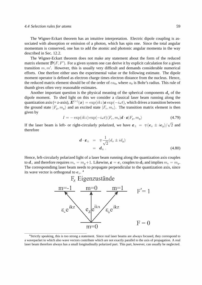
4.4 Selection rules for atoms 59
The Wigner-Eckart theorem has an intuitive interpretation. Electric dipole coupling is as-sociated with absorption or emission of a photon, which has spin one. Since the total angularmomentum is conserved, one has to add the atomic and photonic angular momenta in the waydescribed in Sec. 12.2.
The Wigner-Eckart theorem does not make any statement about the form of the reducedmatrix elementD(F, F ′). For a given system one can derive it by explicit calculation for a giventransitionm,m′. However, this is usually very difficult and demands considerable numericalefforts. One therfore either uses the experimental value or the following estimate. The dipolemoment operator is defined as electron charge times electron distance from the nucleus. Hence,the reduced matrix element should be of the order ofea0, wherea0 is Bohr’s radius. This rule ofthumb gives often very reasonable estimates.
Another important question is the physical meaning of the spherical componentsdq of thedipole moment. To shed light on this we consider a classical laser beam running along thequantization axis (= z-axis),E(+)(x) = exp(ikz)εε exp(−iωt), which drives a transition betweenthe ground state|Fg,mg〉 and an excited state|Fe,me〉. The transition matrix element is thengiven by
I = − exp(ikz) exp(−iωt)〈Fe,me|d · εε|Fg,mg〉 (4.79)
If the laser beam is left- or right-circularly polarized, we haveεε± = ∓(ex ± iey)/√
2 andtherefore
d · εε± = ∓ 1√2(dx ± idy)
= d± . (4.80)
Hence, left-circularly polarized light of a laser beam running along the quantization axis couplestod+ and therefore requiresme = mg+1. Likewise,εε = ez couples tod0 and impliesme = mg.The correspomdimg laser beam needs to propagate perpendicular to the quantization axis, sinceits wave vector is orthogonal toez. 4
4Strictly speaking, this is too strong a statement. Since real laser beams are always focused, they correspond toa wavepacket to which also wave vectors contribute which are not exactly parallel to the axis of propagation. A reallaser beam therefore always has a small longitudinally polarized part. This part, however, can usually be neglected.
60 The Interaction between Atoms and Light
We have to emphasize that circularly polarized light only impliesme = mg ± 1 if the laserbeam propagates along the quantization axis. For another direction the laser light can generallycouple to all spherical componentsdq. For instance, a left-circularly polarized beam along thex-axis has polarizationεε = (−ey − iez)/
√2. Becaused · εε = −id0/
√2 − i(d+ + d−)/2 it
couples to all spherical components, so thatme = mg + i, i = −1, 0, 1 are possible.To conclude this section we summarize the general dipole selection rules, which can be de-
rived from the properties of the Clebsch-Gordan coefficients:∆m = 0,±1∆J = 0,±1ForJ ′ = J the transitionm = 0 → m′ = 0 is forbidden.
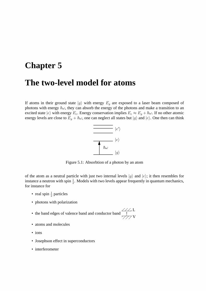
Chapter 5
The two-level model for atoms
If atoms in their ground state|g〉 with energyEg are exposed to a laser beam composed ofphotons with energy~ω, they can absorb the energy of the photons and make a transition to anexcited state|e〉 with energyEe. Energy conservation impliesEe ≈ Eg + ~ω. If no other atomicenergy levels are close toEg + ~ω, one can neglect all states but|g〉 and|e〉. One then can think
|e′〉
|e〉
~ω|g〉
Figure 5.1: Absorbtion of a photon by an atom
of the atom as a neutral particle with just two internal levels|g〉 and |e〉; it then resembles forinstance a neutron with spin1
2. Models with two levels appear frequently in quantum mechanics,
for instance for
• real spin12
particles
• photons with polarization
• the band edges of valence band and conductor bandV
L
• atoms and molecules
• ions
• Josephson effect in superconductors
• interferometer
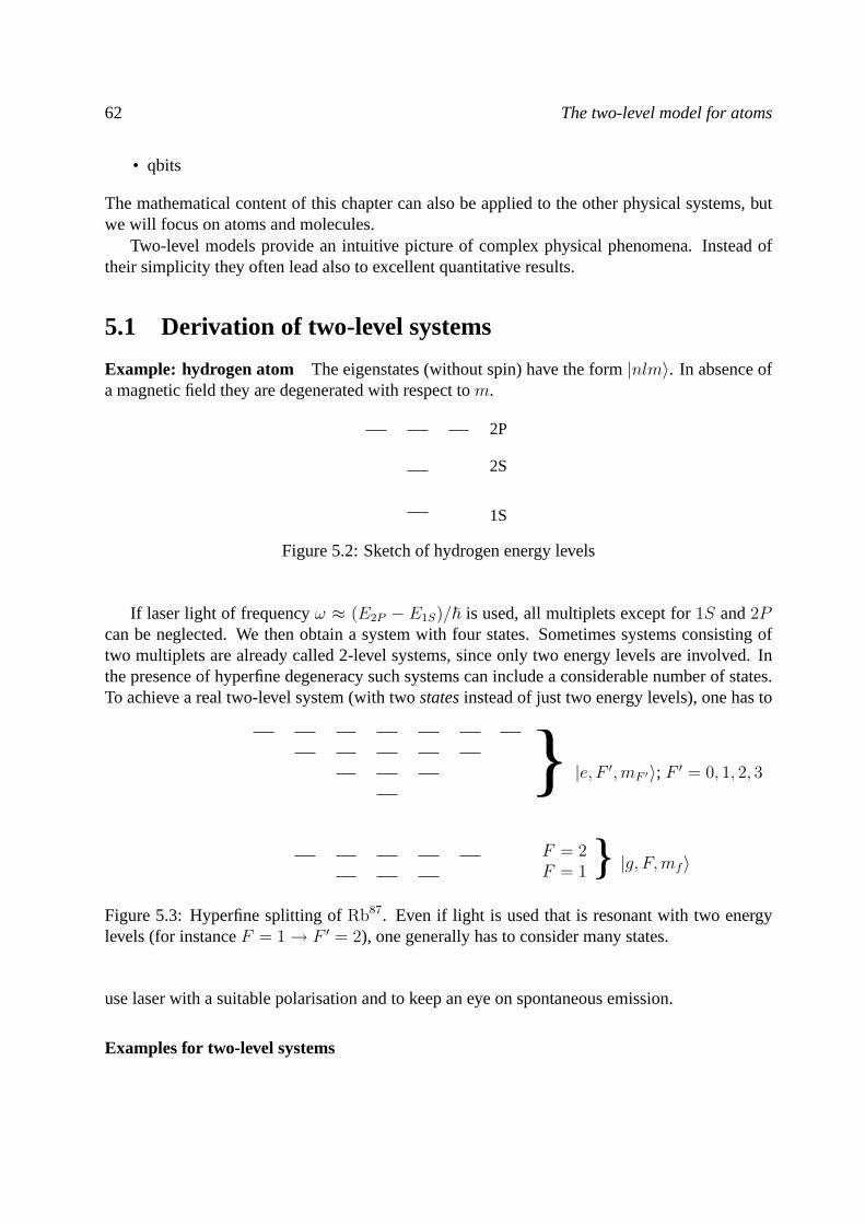
62 The two-level model for atoms
• qbits
The mathematical content of this chapter can also be applied to the other physical systems, butwe will focus on atoms and molecules.
Two-level models provide an intuitive picture of complex physical phenomena. Instead oftheir simplicity they often lead also to excellent quantitative results.
5.1 Derivation of two-level systems
Example: hydrogen atom The eigenstates (without spin) have the form|nlm〉. In absence ofa magnetic field they are degenerated with respect tom.
1S
2P
2S
Figure 5.2: Sketch of hydrogen energy levels
If laser light of frequencyω ≈ (E2P − E1S)/~ is used, all multiplets except for1S and2Pcan be neglected. We then obtain a system with four states. Sometimes systems consisting oftwo multiplets are already called 2-level systems, since only two energy levels are involved. Inthe presence of hyperfine degeneracy such systems can include a considerable number of states.To achieve a real two-level system (with twostatesinstead of just two energy levels), one has to
|e, F ′,mF ′〉; F ′ = 0, 1, 2, 3
F = 2F = 1 |g, F,mf〉
Figure 5.3: Hyperfine splitting ofRb87. Even if light is used that is resonant with two energylevels (for instanceF = 1 → F ′ = 2), one generally has to consider many states.
use laser with a suitable polarisation and to keep an eye on spontaneous emission.
Examples for two-level systems
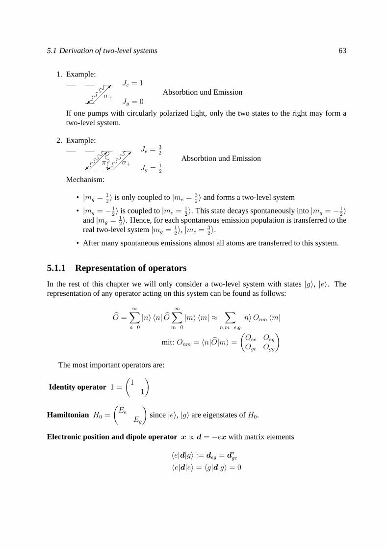
5.1 Derivation of two-level systems 63
1. Example:
Jg = 0
Je = 1Absorbtion und Emissionσ+
If one pumps with circularly polarized light, only the two states to the right may form atwo-level system.
2. Example:
Jg = 12
Je = 32
Absorbtion und Emissionσ+π
Mechanism:
• |mg = 12〉 is only coupled to|me = 3
2〉 and forms a two-level system
• |mg = −12〉 is coupled to|me = 1
2〉. This state decays spontaneously into|mg = −1
2〉
and|mg = 12〉. Hence, for each spontaneous emission population is transferred to the
real two-level system|mg = 12〉, |me = 3
2〉.
• After many spontaneous emissions almost all atoms are transferred to this system.
5.1.1 Representation of operators
In the rest of this chapter we will only consider a two-level system with states|g〉, |e〉. Therepresentation of any operator acting on this system can be found as follows:
O =∞∑n=0
|n〉 〈n| O∞∑m=0
|m〉 〈m| ≈∑
n,m=e,g
|n〉Onm 〈m|
mit: Onm = 〈n|O|m〉 =
(Oee Oeg
Oge Ogg
)The most important operators are:
Identity operator 1 =
(1
1
)
Hamiltonian H0 =
(Ee
Eg
)since|e〉, |g〉 are eigenstates ofH0.
Electronic position and dipole operator x ∝ d = −ex with matrix elements
〈e|d|g〉 := deg = d∗ge
〈e|d|e〉 = 〈g|d|g〉 = 0
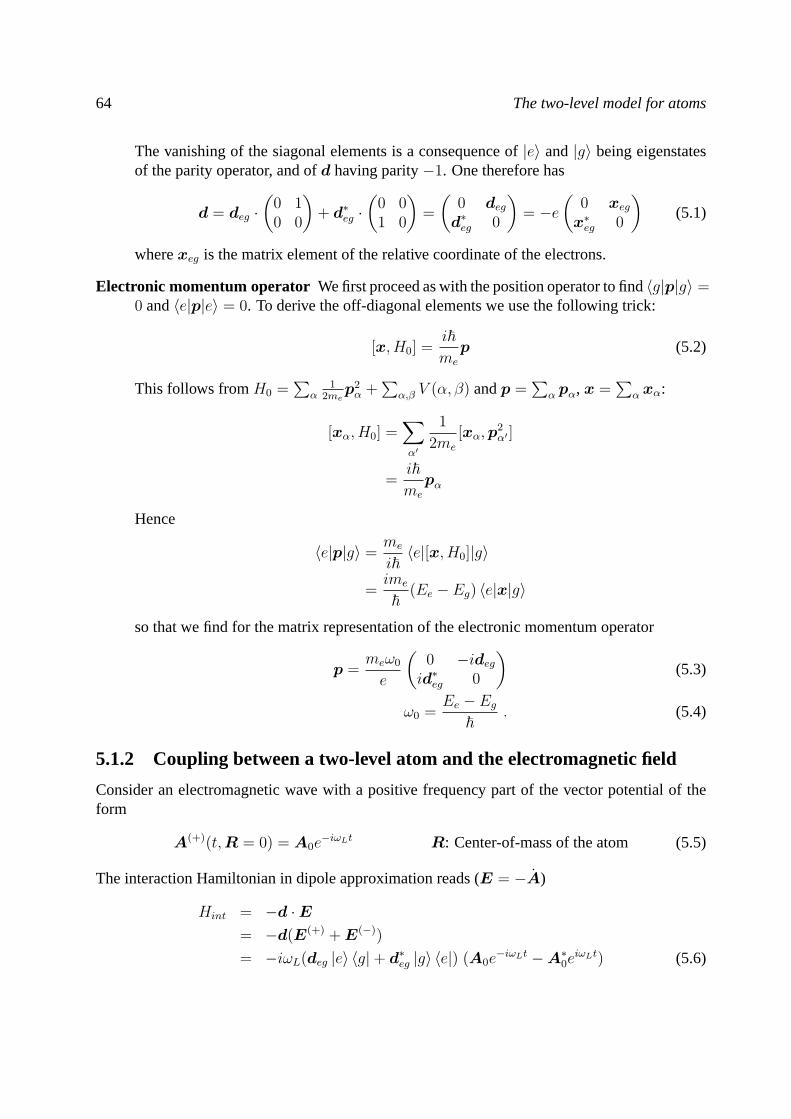
64 The two-level model for atoms
The vanishing of the siagonal elements is a consequence of|e〉 and|g〉 being eigenstatesof the parity operator, and ofd having parity−1. One therefore has
d = deg ·(
0 10 0
)+ d∗eg ·
(0 01 0
)=
(0 deg
d∗eg 0
)= −e
(0 xeg
x∗eg 0
)(5.1)
wherexeg is the matrix element of the relative coordinate of the electrons.
Electronic momentum operator We first proceed as with the position operator to find〈g|p|g〉 =0 and〈e|p|e〉 = 0. To derive the off-diagonal elements we use the following trick:
[x, H0] =i~me
p (5.2)
This follows fromH0 =∑
α1
2mep2α +
∑α,β V (α, β) andp =
∑α pα, x =
∑α xα:
[xα, H0] =∑α′
1
2me
[xα,p2α′ ]
=i~me
pα
Hence
〈e|p|g〉 =me
i~〈e|[x, H0]|g〉
=ime
~(Ee − Eg) 〈e|x|g〉
so that we find for the matrix representation of the electronic momentum operator
p =meω0
e
(0 −idegid∗eg 0
)(5.3)
ω0 =Ee − Eg
~. (5.4)
5.1.2 Coupling between a two-level atom and the electromagnetic field
Consider an electromagnetic wave with a positive frequency part of the vector potential of theform
A(+)(t,R = 0) = A0e−iωLt R: Center-of-mass of the atom (5.5)
The interaction Hamiltonian in dipole approximation reads (E = −A)
Hint = −d ·E= −d(E(+) + E(−))
= −iωL(deg |e〉 〈g|+ d∗eg |g〉 〈e|) (A0e−iωLt −A∗0e
iωLt) (5.6)
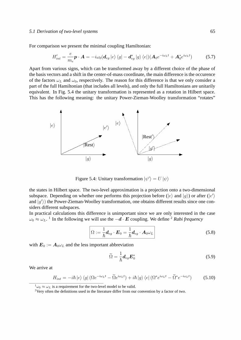
5.1 Derivation of two-level systems 65
For comparison we present the minimal coupling Hamiltonian:
H ′int =e
me
p ·A = −iω0(deg |e〉 〈g| − d∗eg |g〉 〈e|)(A0e−iωLt + A∗0e
iωLt) (5.7)
Apart from various signs, which can be transformed away by a different choice of the phase ofthe basis vectors and a shift in the center-of-mass coordinate, the main difference is the occurenceof the factorsωL andω0, respectively. The reason for this difference is that we only consider apart of the full Hamiltonian (that includes all levels), and only the full Hamiltonians are unitarilyequivalent. In Fig. 5.4 the unitary transformation is represented as a rotation in Hilbert space.This has the following meaning: the unitary Power-Zieman-Woolley transformation “rotates”
|g〉
|Rest〉
|e〉
|g〉
|g′〉
|e〉|e′〉
|Rest′〉
Figure 5.4: Unitary transformation|ψ′〉 = U |ψ〉
the states in Hilbert space. The two-level approximation is a projection onto a two-dimensionalsubspace. Depending on whether one performs this projection before (|e〉 and|g〉) or after (|e′〉and|g′〉) the Power-Zieman-Woolley transformation, one obtains different results since one con-siders different subspaces.In practical calculations this difference is unimportant since we are only interested in the caseω0 ≈ ωL. 1 In the following we will use the−d ·E coupling. We define2 Rabi frequency
Ω :=1
~deg ·E0 =
1
~deg ·A0ωL (5.8)
with E0 := A0ωL and the less important abbreviation
Ω =1
~degE
∗0 (5.9)
We arrive at
Hint = −i~ |e〉 〈g| (Ωe−iωLt − ΩeiωLt) + i~ |g〉 〈e| (Ω∗eiωLt − Ω∗e−iωLt) (5.10)
1ω0 ≈ ωL is a requirement for the two-level model to be valid.2Very often the definitions used in the literature differ from our convention by a factor of two.
66 The two-level model for atoms
The unperturbed Hamiltonian is given by
H0 =
(Ee 00 Eg
)=
1
2(Ee + Eg)1 +
1
2(Ee − Eg)σz (5.11)
By choosing a particular value forEg (the zero-point of energy can be chosen at will) one canrepresentH0 in various ways:
Ee + Eg = 0 ⇒ H0 =~ω0
2σz, ω0 =
Ee − Eg~
(5.12)
Eg = 0 ⇒ H0 = (Ee − Eg)
(1 00 0
)= ~ω0
(1 00 0
)(5.13)
We will frequently make use of therotating-wave approximation. This is a widely used andwell-justified approximation which considerably simplifies calculations. To derive it, we firstswitch to the interaction picture. Thereby the temporal evolution associated withH0 is alreadyincorporated in the wave function:
|ψ〉 = e−iH0t/~ |ψ〉 = U |ψ〉 (5.14)
The transformed Schrodinger equation becomesi~ |˜ψ〉 = H |ψ〉 and the Hamiltonian is trans-formed according to
H = −i~U †U + U †(H0 +Hint)U = U †HintU
= −i~ |e〉 〈g| (Ωe−i(ωL−ω0)t − Ωei(ωL+ω0)t) + H.c.(5.15)
The termei(ωL+ω0)t is fastly oscillating and therefore averages to zero during the evolution. Thisleads to the following simple form of the Hamiltonian in interaction picture,
HWW (t) = −i~e−i∆ tΩ |e〉 〈g|+ i~Ω∗ei∆ t |g〉 〈e| (5.16)
where we have used the laser’s detuning∆ = ωL − ω0.Transforming back to the Schrodinger picture we find
H =~ω0
2σz + ~
(0 −iΩe−iωLt
iΩ∗eiωLt 0
)(5.17)
By another unitary transformation we can achieve thatH only depends on the absolute valueof Ω. This transformation is achieved by multiplying|e〉 with a phase factoreiϕ, where−iΩ =|Ω|eiϕ.
U : |e〉 → eiϕ |e〉
U =
(eiϕ 00 1
)(5.18)
This leads to the final and simple form for the Hamiltonian,
U †HU =~ω0
2σz + ~
(0 |Ω|e−iωLt
|Ω|eiωLt 0
)(5.19)
5.2 Rabi oscillations and Landau-Zener transitions 67
5.2 Rabi oscillations and Landau-Zener transitions
We will now deal with the time evolution of a state with HamiltonianH as discussed in theprevious section.
i~∂t(ψeψg
)= ~
(ω0
2−iΩe−iωLt
iΩ∗eiωLt −ω0
2
)(ψeψg
)(5.20)
Without the time dependent factoreiωLt this equation would be easily solvable. Luckily, we canremoce this factor by a unitary transformation:
U = e−iωL2σzt =
(e−i
ωL2t 0
0 eiωL2t
) (ψeψg
)= U
(ψeψg
)(5.21)
The transformed equation becomes
i~∂t
(ψeψg
)=
(−i~U †U + U †HU
)(ψeψg
)
=− ~ωL
2σz +
~ω0
2σz + ~
(0 −iΩiΩ∗ 0
)(ψeψg
)(5.22)
We therefore find forH:
H = ~(−∆
2−iΩ
iΩ∗ ∆2
)(5.23)
Such a time-independent Hamiltonian is only possible in rotating-wave approximation. Thecounter-rotating terms would still depend on time after transformation Eq. (5.21). We now caneasily solve the Schrodinger equation:(
ψe(t)
ψg(t)
)= e−it
eH/~(ψe(0)
ψg(0)
)(5.24)
Let us now rewriteH. Since the Hamiltonian is Hermitean and traceless, there are only threeindependent parameters.
H = ~n · σ, n =
ImΩReΩ−∆
2
(5.25)
The expressione−itn·σ can be expanded into a Taylor series,
e−itn·σ =∞∑l=0
1
l!(−it)l(n · σ)l (5.26)
68 The two-level model for atoms
The product of twoσ matrices is given by
σiσj = iεijkσk + δij1 (5.27)
⇒ (n · σ)2 = niσinjσj = ninj(iεijkσk + δij1) = |n|21 (5.28)
(n · σ)2l = |n|2l1 (5.29)
We thus can bringe−itn·σ into the form
e−itn·σ =∞∑l=0
(−it)2l
(2l)!(n · σ)2l +
∞∑l=0
(−it)2l+1
(2l + 1)!(n · σ)2l+1 (5.30)
e−itn·σ = cos(|n|t)1− in · σ|n|
sin(|n|t) (5.31)
We introduce the notation
w := |n| =
√(∆
2
)2
+ |Ω|2 (5.32)
which only depends on the modulus ofΩ. For an atom that initially is in its ground state, thesolution becomes(
ψe(0)
ψg(0)
)=
(01
)⇒
(ψe(t)
ψg(t)
)=
(−Ω
wsin(wt)
cos(wt)− i ∆2w
sin(wt)
)(5.33)
The probability amplitudeψe(t) to excite an atom oscillates with frequencyw, this phenomenonis calledRabi oscillations. We have
Pe(t) = |ψe(t)|2 =|Ω|2
w2sin2(wt) (5.34)
The maximum value ofPe is reached forwt = π/2 + nπ and given by
Pe ∝|Ω|2
(∆2)2 + |Ω|2
(5.35)
If the laser is not detuned against the resonance frequency,∆ = 0, complete excitation (Pe = 1)is possible.Pe depends strongly on the detuning,
∆ |Ω| ⇒ Pe ≈|Ω|2
∆2 1 (5.36)
The excitation probability therefore depends on the ratio of Rabi frequency and detuning.3
These results are of very high relevance for atom optics, quantum optics, electron spin resonance,nuclear spin resonance, Interferometry, and many other areas.
3It is often claimed that the excitation probability depends on the ratio of Rabi frequency and spontaneousemission rate. We will see later that this ratio is also important for small detunings. The ratio ofΩ/∆ is usuallymore important, though.
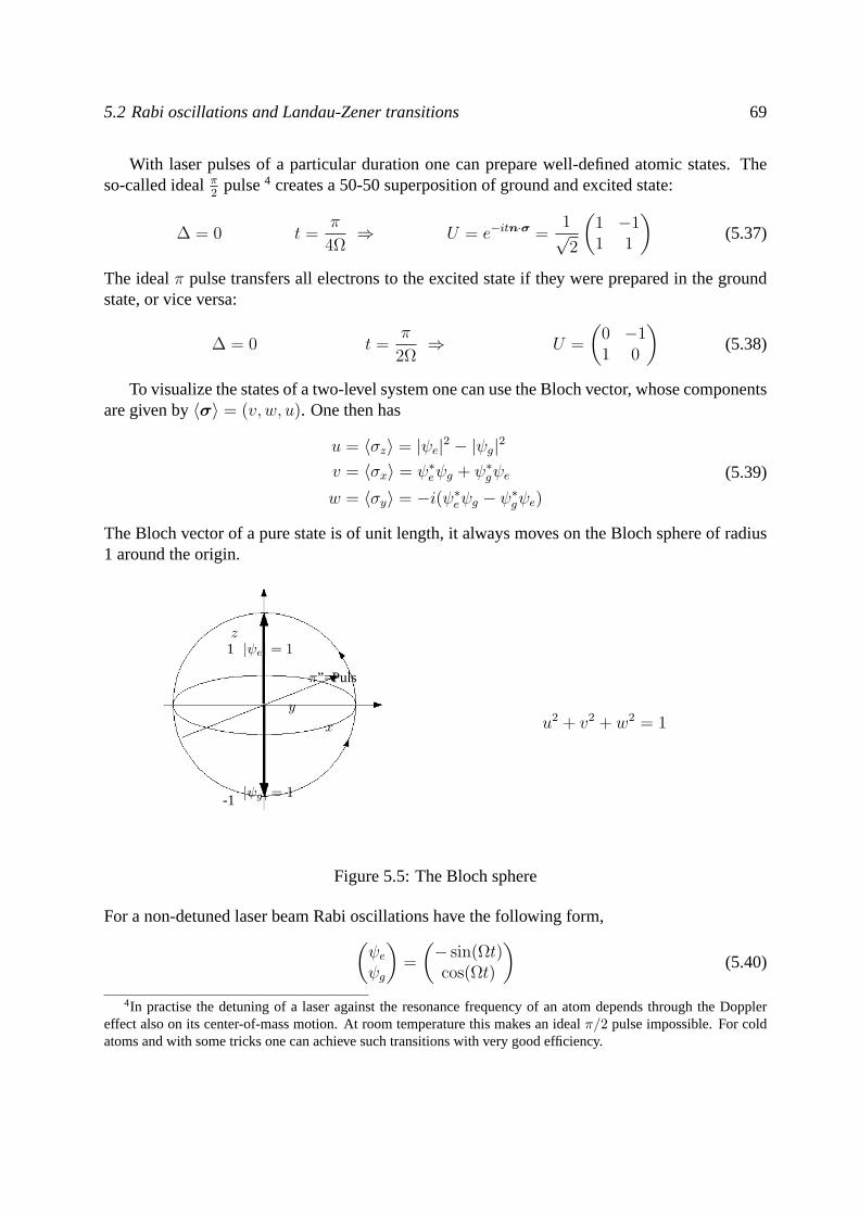
5.2 Rabi oscillations and Landau-Zener transitions 69
With laser pulses of a particular duration one can prepare well-defined atomic states. Theso-called idealπ
2pulse4 creates a 50-50 superposition of ground and excited state:
∆ = 0 t =π
4Ω⇒ U = e−itn·σ =
1√2
(1 −11 1
)(5.37)
The idealπ pulse transfers all electrons to the excited state if they were prepared in the groundstate, or vice versa:
∆ = 0 t =π
2Ω⇒ U =
(0 −11 0
)(5.38)
To visualize the states of a two-level system one can use the Bloch vector, whose componentsare given by〈σ〉 = (v, w, u). One then has
u = 〈σz〉 = |ψe|2 − |ψg|2
v = 〈σx〉 = ψ∗eψg + ψ∗gψe
w = 〈σy〉 = −i(ψ∗eψg − ψ∗gψe)
(5.39)
The Bloch vector of a pure state is of unit length, it always moves on the Bloch sphere of radius1 around the origin.
-1|ψg| = 1
1z|ψe| = 1
y
x
π”=Puls
u2 + v2 + w2 = 1
Figure 5.5: The Bloch sphere
For a non-detuned laser beam Rabi oscillations have the following form,(ψeψg
)=
(− sin(Ωt)cos(Ωt)
)(5.40)
4In practise the detuning of a laser against the resonance frequency of an atom depends through the Dopplereffect also on its center-of-mass motion. At room temperature this makes an idealπ/2 pulse impossible. For coldatoms and with some tricks one can achieve such transitions with very good efficiency.
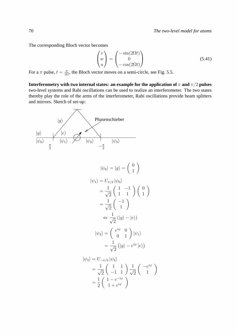
70 The two-level model for atoms
The corresponding Bloch vector becomesvwu
=
− sin(2Ωt)0
− cos(2Ωt)
(5.41)
For aπ pulse,t = π2Ω
, the Bloch vector moves on a semi-circle, see Fig. 5.5.
Interferometry with two internal states: an example for the application of π and π/2 pulsestwo-level systems and Rabi oscillations can be used to realize an interferometer. The two statesthereby play the role of the arms of the interferometer, Rabi oscillations provide beam splittersand mirrors. Sketch of set-up:
|ψ0〉 |ψ1〉π2
|ψ2〉 |ψ3〉|g〉
|g〉
|e〉
−π2
Phasenschieber
|ψ0〉 = |g〉 =
(01
)|ψ1〉 = Uπ/2 |ψ0〉
=1√2
(1 −11 1
)(01
)=
1√2
(−11
)⇔ 1√
2(|g〉 − |e〉)
|ψ2〉 =
(eiϕ 00 1
)|ψ1〉
=1√2
(|g〉 − eiϕ |e〉
)|ψ3〉 = U−π/2 |ψ2〉
=1√2
(1 1−1 1
)1√2
(−eiϕ
1
)=
1
2
(1− e−iϕ
1 + eiϕ
)
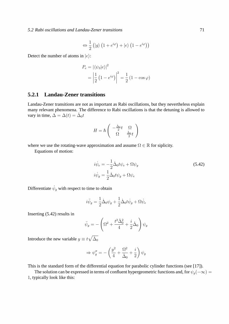
5.2 Rabi oscillations and Landau-Zener transitions 71
⇔ 1
2
(|g〉(1 + eiϕ
)+ |e〉
(1− eiϕ
))Detect the number of atoms in|e〉:
Pe = |〈ψ3|e〉|2
=
∣∣∣∣12 (1− eiϕ)∣∣∣∣2 =
1
2(1− cosϕ)
5.2.1 Landau-Zener transitions
Landau-Zener transitions are not as important as Rabi oscillations, but they nevertheless explainmany relevant phenomena. The difference to Rabi oscillations is that the detuning is allowed tovary in time,∆ = ∆(t) = ∆0t
H = ~
(− ∆0
2t Ω
Ω ∆0
2t
)
where we use the rotating-wave approximation and assumeΩ ∈ R for siplicity.Equations of motion:
iψe = −1
2∆0tψe + Ωψg (5.42)
iψg =1
2∆0tψg + Ωψe
Differentiateψg with respect to time to obtain
iψg =1
2∆0ψg +
1
2∆0tψg + Ωψe
Inserting (5.42) results in
ψg = −
(Ω2 +
t2∆20
4+i
2∆0
)ψg
Introduce the new variabley ≡ t√
∆0
⇒ ψ′′g = −(y2
4+
Ω2
∆0
+i
2
)ψg
This is the standard form of the differential equation for parabolic cylinder functions (see [17]).The solution can be expressed in terms of confluent hypergeometric functions and, forψg(−∞) =
1, typically look like this:
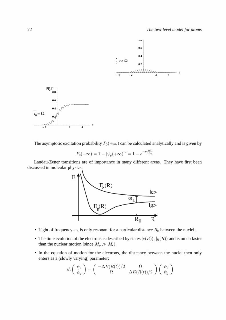
72 The two-level model for atoms
The asymptotic excitation probabilityP0(+∞) can be calculated analytically and is given by
P0(+∞) = 1− |ψg(+∞)|2 = 1− e−π Ω2
2∆0
Landau-Zener transitions are of importance in many different areas. They have first beendiscussed in moleular physics:
• Light of frequencyωL is only resonant for a particular distanceR0 between the nuclei.
• The time evolution of the electrons is described by states|e(R)〉, |g(R)〉 and is much fasterthan the nuclear motion (sinceMp Me)
• In the equation of motion for the electrons, the distcance between the nuclei then onlyenters as a (slowly varying) parameter:
i~(ψeψg
)=
(−∆E(R(t))/2 Ω
Ω ∆E(R(t))/2
)(ψeψg
)
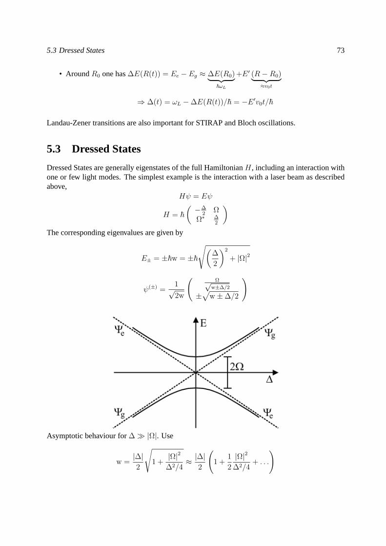
5.3 Dressed States 73
• AroundR0 one has∆E(R(t)) = Ee − Eg ≈ ∆E(R0)︸ ︷︷ ︸~ωL
+E ′ (R−R0)︸ ︷︷ ︸≈v0t
⇒ ∆(t) = ωL −∆E(R(t))/~ = −E ′v0t/~
Landau-Zener transitions are also important for STIRAP and Bloch oscillations.
5.3 Dressed States
Dressed States are generally eigenstates of the full HamiltonianH, including an interaction withone or few light modes. The simplest example is the interaction with a laser beam as describedabove,
Hψ = Eψ
H = ~(−∆
2Ω
Ω∗ ∆2
)The corresponding eigenvalues are given by
E± = ±~w = ±~
√(∆
2
)2
+ |Ω|2
ψ(±) =1√2w
(Ω√
w±∆/2
±√
w ±∆/2
)
Asymptotic behaviour for∆ |Ω|. Use
w =|∆|2
√1 +
|Ω|2
∆2/4≈ |∆|
2
(1 +
1
2
|Ω|2
∆2/4+ . . .
)
74 The two-level model for atoms
ψ(+)e →
0 ∆ →∞1 ∆ → −∞
ψ(−)e →
1 ∆ →∞0 ∆ → −∞
This phenomenon is called “avoided crossing”: ForΩ = 0 the eigenstates areψe andψg; theireigenvalues are crossing at∆ = 0. For Ω 6= 0, the coupling of the states by the laser beamtransforms this crossing into two non-intersecting hyperbolas with minimum enerhy distance2~ |Ω|.
It is remarkable that, if one follows one of the hyperbolas, one evolves forE− fromψg toψe,and forE+ from ψe to ψg. This means that, for time-dependent∆(t), one can make a transitionfrom ψg to ψe while always staying in an instantaneous eigenstate ofH(t) (see also the sectionon the adiabatic theorem below).
This behaviour is closely related to Landau-Zener transitions. tunneling betweenE− andE+
corresponds to not exciting the atoms. For a slow rate of change an atom tries to stay on one ofthe hyperbolas for a Landau-Zener transition.
The asymptotic transition probability can also be understood by estimating the tunnelingprobability between the two hyperbolas. According to the WKB approximation (see, e.g., Ref. [18]),the tunneling probability between the hyperbolas can be expressed asP = e−∆Et/~, with ∆E
~ =2 |Ω|. The typical time scalet for tunneling can be estimated by the time when the distancebetween the two energy levels has grown to4 |Ω|.
⇔ 4 |Ω|2 =
(∆(t)
2
)2
+ |Ω|2
⇒ ∆ = ∆0t ≈ 4 |Ω|
⇒ t =4 |Ω|∆0
⇒ P = e− 2|Ω|4|Ω|
∆0 = e− 8|Ω|2
∆0
5.3.1 Dressed states in a cavity
The notion of a dressed states is more frequently used if the atoms are coupled to the quantizedradiation field. The form of the corresponding two-level Hamiltonian can be derived as before.The only difference is that the Rabi frequency becomes an operator:
Ω =1
~deg · E
(+)(x) (5.43)
This results in the Hamilton operator
H =~ω0
2σz −
[deg · E(x) |e〉 〈g|+ d∗eg · E(x) |g〉 〈e|
]+Hrad (5.44)
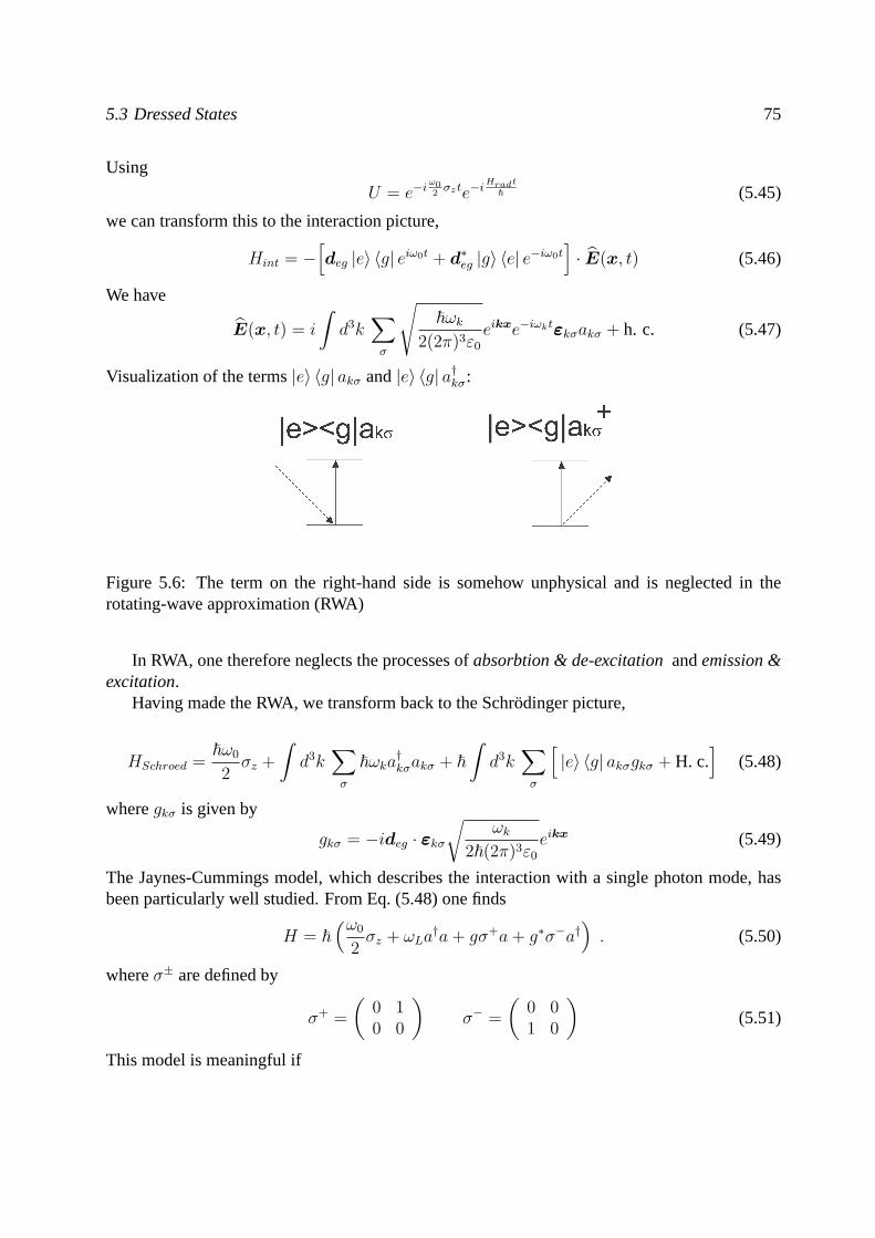
5.3 Dressed States 75
Using
U = e−iω02σzte−i
Hradt
~ (5.45)
we can transform this to the interaction picture,
Hint = −[deg |e〉 〈g| eiω0t + d∗eg |g〉 〈e| e−iω0t
]· E(x, t) (5.46)
We have
E(x, t) = i
∫d3k
∑σ
√~ωk
2(2π)3ε0
eikxe−iωktεεkσakσ + h. c. (5.47)
Visualization of the terms|e〉 〈g| akσ and|e〉 〈g| a†kσ:
Figure 5.6: The term on the right-hand side is somehow unphysical and is neglected in therotating-wave approximation (RWA)
In RWA, one therefore neglects the processes ofabsorbtion & de-excitationandemission &excitation.
Having made the RWA, we transform back to the Schrodinger picture,
HSchroed =~ω0
2σz +
∫d3k
∑σ
~ωka†kσakσ + ~∫d3k
∑σ
[|e〉 〈g| akσgkσ + H. c.
](5.48)
wheregkσ is given by
gkσ = −ideg · εεkσ√
ωk2~(2π)3ε0
eikx (5.49)
The Jaynes-Cummings model, which describes the interaction with a single photon mode, hasbeen particularly well studied. From Eq. (5.48) one finds
H = ~(ω0
2σz + ωLa
†a+ gσ+a+ g∗σ−a†). (5.50)
whereσ± are defined by
σ+ =
(0 10 0
)σ− =
(0 01 0
)(5.51)
This model is meaningful if
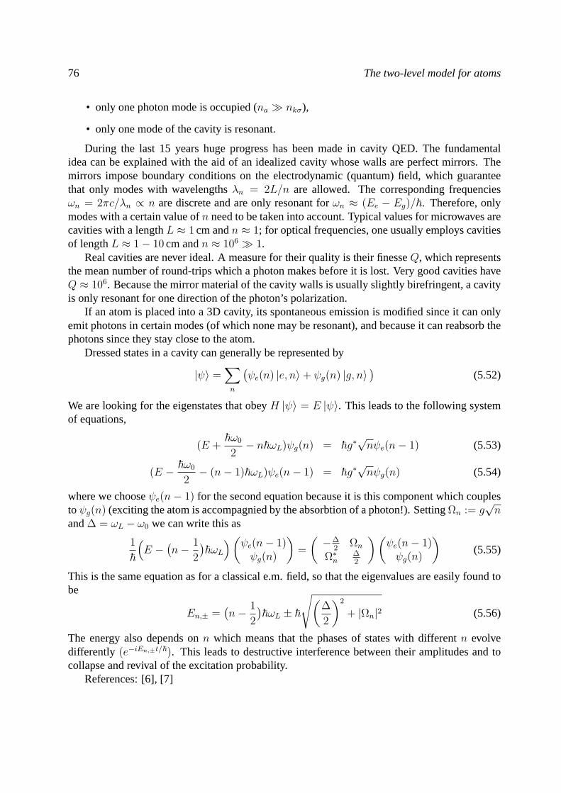
76 The two-level model for atoms
• only one photon mode is occupied (na nkσ),
• only one mode of the cavity is resonant.
During the last 15 years huge progress has been made in cavity QED. The fundamentalidea can be explained with the aid of an idealized cavity whose walls are perfect mirrors. Themirrors impose boundary conditions on the electrodynamic (quantum) field, which guaranteethat only modes with wavelengthsλn = 2L/n are allowed. The corresponding frequenciesωn = 2πc/λn ∝ n are discrete and are only resonant forωn ≈ (Ee − Eg)/~. Therefore, onlymodes with a certain value ofn need to be taken into account. Typical values for microwaves arecavities with a lengthL ≈ 1 cm andn ≈ 1; for optical frequencies, one usually employs cavitiesof lengthL ≈ 1− 10 cm andn ≈ 106 1.
Real cavities are never ideal. A measure for their quality is their finesseQ, which representsthe mean number of round-trips which a photon makes before it is lost. Very good cavities haveQ ≈ 106. Because the mirror material of the cavity walls is usually slightly birefringent, a cavityis only resonant for one direction of the photon’s polarization.
If an atom is placed into a 3D cavity, its spontaneous emission is modified since it can onlyemit photons in certain modes (of which none may be resonant), and because it can reabsorb thephotons since they stay close to the atom.
Dressed states in a cavity can generally be represented by
|ψ〉 =∑n
(ψe(n) |e, n〉+ ψg(n) |g, n〉
)(5.52)
We are looking for the eigenstates that obeyH |ψ〉 = E |ψ〉. This leads to the following systemof equations,
(E +~ω0
2− n~ωL)ψg(n) = ~g∗
√nψe(n− 1) (5.53)
(E − ~ω0
2− (n− 1)~ωL)ψe(n− 1) = ~g∗
√nψg(n) (5.54)
where we chooseψe(n− 1) for the second equation because it is this component which couplestoψg(n) (exciting the atom is accompagnied by the absorbtion of a photon!). SettingΩn := g
√n
and∆ = ωL − ω0 we can write this as
1
~
(E −
(n− 1
2
)~ωL
)(ψe(n− 1)ψg(n)
)=
(−∆
2Ωn
Ω∗n∆2
)(ψe(n− 1)ψg(n)
)(5.55)
This is the same equation as for a classical e.m. field, so that the eigenvalues are easily found tobe
En,± =(n− 1
2
)~ωL ± ~
√(∆
2
)2
+ |Ωn|2 (5.56)
The energy also depends onn which means that the phases of states with differentn evolvedifferently (e−iEn,±t/~). This leads to destructive interference between their amplitudes and tocollapse and revival of the excitation probability.
References: [6], [7]
5.4 Models with few levels, dark states, Raman transitions 77
5.4 Models with few levels, dark states, Raman transitions
The most common extension of the two-level model is of course the three-level model. Such asystem can be achieved by choosing lasers in a suitable way. An example are transitions fromJ = 1 to J ′ = 1, where the transition fromJ ′ to J with m = m′ = 0 is forbidden by a selectionrule. Shining two laser beams with polarizationσ+ andσ− on the atom therefore depopulates thestatem = 0, J = 1. After this has happened, one obtains a so-calledΛ system consisting of thestates|J = 1,m = ±1〉 and|J ′ = 1,m′ = 0〉.
Figure 5.7: The arrows represent the transitions which are driven by theσ± light. The eavy linesrepresent de-excitation due to spontaneous emission.
The Hamilton operator of this system in RWA reads
H =
Ee ~Ω+e−iω+t ~Ω−e
−iω−t
~Ω∗+eiω+t E+ 0
~Ω∗−eiω−t 0 E−
= Ee1 +
0 ~Ω+e−iω+t ~Ω−e
−iω−t
~Ω∗+eiω+t E+ − Ee 0
~Ω∗−e−iω−t 0 E− − Ee
(5.57)
Again we perform a unitary transformation which removes any time dependence fromH:
ψ± = e−iω±tψ± (5.58)
This leads to the time-independent Hamiltonian
H = ~
0 Ω+ Ω−Ω∗+ ∆+ 0Ω∗− 0 ∆−
+ Ee1 (5.59)
where we have set∆± = ω± − Ee−E±~ .
5.4.1 Dark States
Consider the case oftwo photon resonance: ∆+ = ∆−. This means that for∆± 6= 0 theindividual photons are not in resonance with the respective transitions|±〉 → |e〉. However, wehave~(ω+ − ω−) = E− − E+ which follows from∆+ = ∆− because of wegen
~ω+ − Ee + E+ = ~ω− − Ee + E−
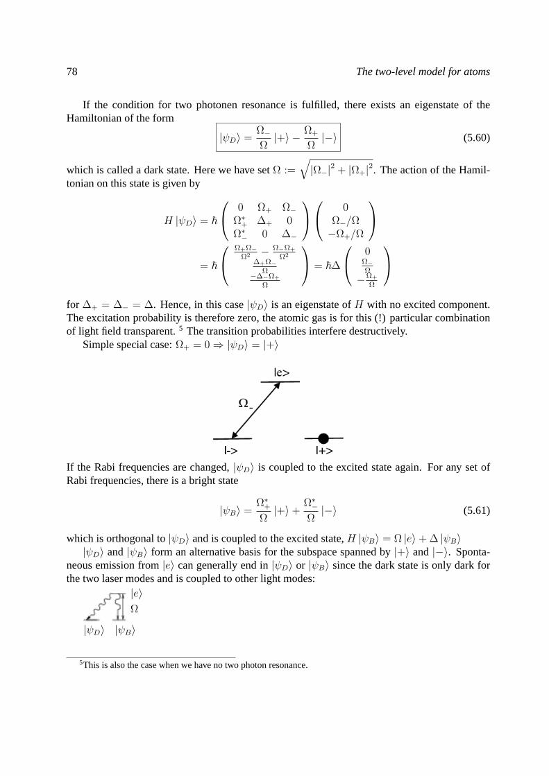
78 The two-level model for atoms
If the condition for two photonen resonance is fulfilled, there exists an eigenstate of theHamiltonian of the form
|ψD〉 =Ω−Ω|+〉 − Ω+
Ω|−〉 (5.60)
which is called a dark state. Here we have setΩ :=√|Ω−|2 + |Ω+|2. The action of the Hamil-
tonian on this state is given by
H |ψD〉 = ~
0 Ω+ Ω−Ω∗+ ∆+ 0Ω∗− 0 ∆−
0Ω−/Ω−Ω+/Ω
= ~
Ω+Ω−Ω2 − Ω−Ω+
Ω2
∆+Ω−Ω
−∆−Ω+
Ω
= ~∆
0Ω−Ω
−Ω+
Ω
for ∆+ = ∆− = ∆. Hence, in this case|ψD〉 is an eigenstate ofH with no excited component.The excitation probability is therefore zero, the atomic gas is for this (!) particular combinationof light field transparent.5 The transition probabilities interfere destructively.
Simple special case:Ω+ = 0 ⇒ |ψD〉 = |+〉
If the Rabi frequencies are changed,|ψD〉 is coupled to the excited state again. For any set ofRabi frequencies, there is a bright state
|ψB〉 =Ω∗+Ω|+〉+
Ω∗−Ω|−〉 (5.61)
which is orthogonal to|ψD〉 and is coupled to the excited state,H |ψB〉 = Ω |e〉+ ∆ |ψB〉|ψD〉 and|ψB〉 form an alternative basis for the subspace spanned by|+〉 and|−〉. Sponta-
neous emission from|e〉 can generally end in|ψD〉 or |ψB〉 since the dark state is only dark forthe two laser modes and is coupled to other light modes:
|ψB〉|ψD〉
|e〉Ω
5This is also the case when we have no two photon resonance.
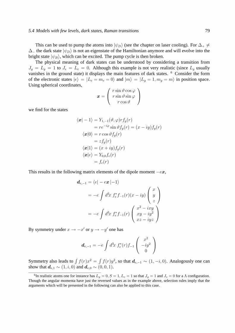
5.4 Models with few levels, dark states, Raman transitions 79
This can be used to pump the atoms into|ψD〉 (see the chapter on laser cooling). For∆+ 6=∆− the dark state|ψD〉 is not an eigenstate of the Hamiltonian anymore and will evolve into thebright state|ψB〉, which can be excited. The pump cycle is then broken.
The physical meaning of dark states can be understood by considering a transition fromJg = Lg = 1 to Je = Le = 0. Although this example is not very realistic (sinceLg usuallyvanishes in the ground state) it displays the main features of dark states.6 Consider the formof the electronic states|e〉 = |Le = me = 0〉 and |m〉 = |Lg = 1,mg = m〉 in position space.Using spherical coordinates,
x =
r sinϑ cosϕr sinϑ sinϕr cosϑ
we find for the states
〈x| − 1〉 = Y1,−1(ϑ, ϕ)rfg(r)
= re−iϕ sinϑfg(r) = (x− iy)fg(r)
〈x|0〉 = r cosϑfg(r)
= zfg(r)
〈x|1〉 = (x+ iy)fg(r)
〈x|e〉 = Y0,0fe(r)
= fe(r)
This results in the following matrix elements of the dipole moment−ex,
de,−1 = 〈e| − ex |−1〉
= −e∫d3x f ∗e f−1(r)(x− iy)
xyz
= −e
∫d3x f ∗e f−1(r)
x2 − ixyxy − iy2
xz − iyz
By symmetry underx→ −x′ or y → −y′ one has
de,−1 = −e∫d3x f ∗e (r)f−1
x2
−iy2
0
Symmetry also leads to
∫f(r)x2 =
∫f(r)y2, so thatde,−1 ∼ (1,−i, 0). Analogously one can
show thatde,1 ∼ (1, i, 0) andde,0 ∼ (0, 0, 1).
6In realistic atoms one for instance hasLg = 0, S = 1, Le = 1 so thatJg = 1 andJe = 0 for aΛ configuration.Though the angular momenta have just the reversed values as in the example above, selection rules imply that thearguments which will be presented in the following can also be applied to this case.
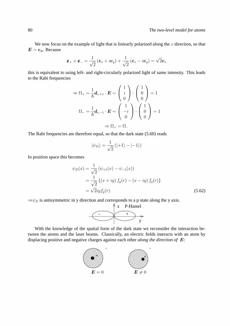
80 The two-level model for atoms
We now focus on the example of light that is liniearly polarized along thex direction, so thatE ∼ ex. Because
εε+ + εε− =1√2
(ex + iey) +1√2
(ex − iey) =√
2ex
this is equivalent to using left- and right-circularly polarized light of same intensity. This leadsto the Rabi frequencies
⇒ Ω+ =1
~de,+1 ·E ∼
1i0
· 1
00
= 1
Ω− =1
~de,−1 ·E ∼
1−i0
· 1
00
= 1
⇒ Ω+ = Ω−
The Rabi frequencies are therefore equal, so that the dark state (5.60) reads
|ψD〉 =1√2
(|+1〉 − |−1〉)
In position space this becomes
ψD(x) =1√2
(ψ+1(x)− ψ−1(x))
=1√2(x+ iy) fg(r)− (x− iy) fg(r)
=√
2iyfg(r) (5.62)
⇒ψD is antisymmetric in y direction and corresponds to a p state along the y axis.
- +
y
x P-Hantel
With the knowledge of the spatial form of the dark state we reconsider the interaction be-tween the atoms and the laser beams. Classically, an electric fields interacts with an atom bydisplacing positive and negative charges against each otheralong the direction ofE:
+ +
- -
E = 0 E 6= 0
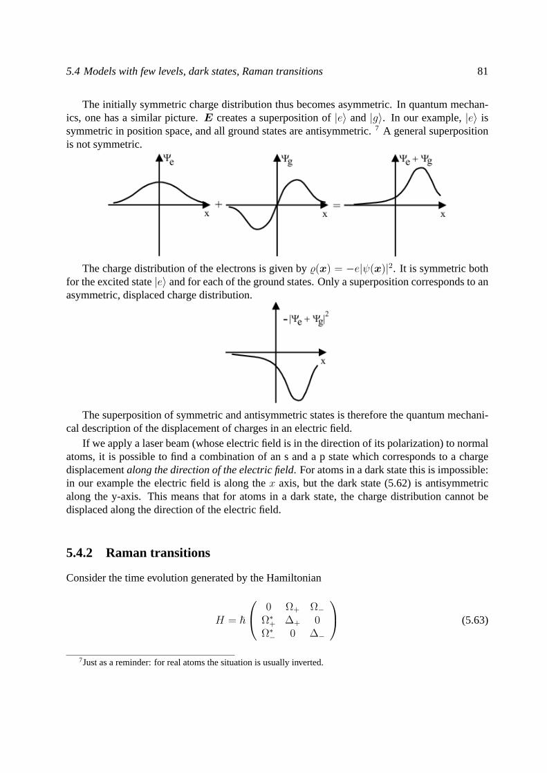
5.4 Models with few levels, dark states, Raman transitions 81
The initially symmetric charge distribution thus becomes asymmetric. In quantum mechan-ics, one has a similar picture.E creates a superposition of|e〉 and |g〉. In our example,|e〉 issymmetric in position space, and all ground states are antisymmetric.7 A general superpositionis not symmetric.
The charge distribution of the electrons is given by%(x) = −e|ψ(x)|2. It is symmetric bothfor the excited state|e〉 and for each of the ground states. Only a superposition corresponds to anasymmetric, displaced charge distribution.
The superposition of symmetric and antisymmetric states is therefore the quantum mechani-cal description of the displacement of charges in an electric field.
If we apply a laser beam (whose electric field is in the direction of its polarization) to normalatoms, it is possible to find a combination of an s and a p state which corresponds to a chargedisplacementalong the direction of the electric field. For atoms in a dark state this is impossible:in our example the electric field is along thex axis, but the dark state (5.62) is antisymmetricalong the y-axis. This means that for atoms in a dark state, the charge distribution cannot bedisplaced along the direction of the electric field.
5.4.2 Raman transitions
Consider the time evolution generated by the Hamiltonian
H = ~
0 Ω+ Ω−Ω∗+ ∆+ 0Ω∗− 0 ∆−
(5.63)
7Just as a reminder: for real atoms the situation is usually inverted.
82 The two-level model for atoms
⇒ iψe = Ω+ψ+ + Ω−ψ−
iψ± = ∆±ψ± + Ω∗±ψe
Ansatz:ψ± = e−i∆±tψ± ⇒
iψe = Ω+e−i∆+tψ+ + Ω−e
−i∆−tψ− (5.64)
i ˙ψ± = Ω∗±ei∆±tψe (5.65)
Since|ψe| ≤ 1 one finds that| ˙ψ±| ≤ |Ω±| holds. The formal solution forψe is given by
ψe(t) = ψe(0)︸ ︷︷ ︸≡0
−i∫ t
0
dt′
Ω+e−i∆+t′ψ+(t′) + Ω−e
−i∆−t′ψ−(t′)
(5.66)
We now focus on the case of large detunings|∆±| |Ω±|. In this case,ψ±(t) varies slowly
compared toe−i∆±t since∣∣∣ ˙ψ±
∣∣∣ ≤ |Ω±| |∆±|. We therefore can setψ±(t′) ≈ ψ±(t) in the
integral, which results in
ψe(t) ≈Ω+
∆+
(e−i∆+t − 1
)ψ+(t) +
Ω−∆−
(e−i∆−t − 1
)ψ−(t)
Inserting this into Eq. (5.65) leads to
i ˙ψ± = Ω∗±ei∆±t
Ω+
∆+
(e−i∆+t − 1
)ψ+(t) +
Ω−∆−
(e−i∆−t − 1
)ψ−(t)
or, explicitly for one component,
i ˙ψ+ =|Ω+|2
∆+
(1− ei∆+t
)︸ ︷︷ ︸≈1
ψ+(t) +Ω∗+Ω−∆−
(ei(∆+−∆−)t − ei∆+t
)︸ ︷︷ ︸≈ei(∆+−∆−)t
ψ−(t)
where fastly oscillating terms average to zero and therefore can be neglected against the slowterms. 8 In summary, we thus can write down an effective two-level description for the twoground states,
i~∂
∂t
(ψ+
ψ−
)= Heff
(ψ+
ψ−
)(5.67)
with
Heff = ~
(|Ω+|2∆+
Ω∗+Ω−∆−
ei(∆+−∆−)t
Ω∗−Ω+
∆+e−i(∆+−∆−)t |Ω−|2
∆−
)(5.68)
8In contrast to this, in Eq. (5.65) we had fast terms only. Hence they produce the dominant effect and cannot beneglected.
5.5 Adiabatc theorem, STIRAP 83
The excited state is never significantly populated and could be omitted in these equations. Thisprocedure is called adiabatic elemination of the excited state.
The matrix elements ofHeff are proportional toΩ2/∆. It is of fundamental importance thatthis expression can be large even when the excitation probabilityPe = Ω2/∆2 is small. Thismakes Raman transitions an excellent tool to coherently manipulate atomic states, since a smallexcitation probability implies that loss of coherence due to spontaneous emission is stronglysuppressed. The time scale of loss of coherence (decoherence) due to spontaneous emission isgiven by the excitation probability times the rate of spontaneous emission,γPe. Typical numbersfor Raman transitions areΩ = 109 Hz,γ = 107 Hz,∆ = 1010 Hz. This results inΩ2/∆ = 108 HzandγPe = 105 Hz.
Theeffective Rabi frequency
Ωeff :=Ω∗+Ω−
∆(5.69)
is a measure for the strength of the coupling between the two ground states. We have omittedthe index± for the detunings, since for∆− 6= ∆+ one runs into the problem thatHeff is notHermitean anymore. However,Heff is nevertheless a very useful operator if one knows why thishappens. The reason is that the adiabatic evolution of the excited state which was discussedabove,
ψe =Ω+
∆+
ψ+
(e−i∆+t − 1
)+
Ω−∆−
ψ−(e−i∆−t − 1
)(5.70)
is actually the first order term of a Taylor expansion ofψe with respect to 1∆±
. Thus,ψe is only
correct to first order in 1∆±
, if all other frequencies in the Hamiltonian,Ω±, ∆+ − ∆− ∆±,are much smaller than the detunings. This implies that we have to do the following expansion:
1
∆−=
1
(∆− −∆+) + ∆+
≈ 1
∆+
− 1
∆2+
(∆− −∆+) + . . . (5.71)
=1
∆+
+O((1
∆2+
)) (5.72)
This means that to first order the expressions1/∆± are the same,Heff is therefore Hermitean tofirst order in 1
∆±. Introducing the effective Rabi frequency as in (5.69), one can representHeff as
Heff = ~(
∗ Ωeffei(∆+−∆−)t
Ω∗effe−i(∆+−∆−)t ∗
)(5.73)
This Hamiltonian is analogous to that that of a two-level system.
5.5 Adiabatc theorem, STIRAP
The method ofSTImulatedRapid AdiabaticPassage is a highly efficient tool of coherent ma-nipulation which combines dark states and Raman transitions. It is based on the
84 The two-level model for atoms
Adiabatic theorem: LetH(t) be a time-dependent Hamiltonian with instantaneous eigenstates|n(t)〉,H(t) |n(t)〉 = En(t) |n(t)〉. Then the evolution of a state|ψ(t)〉, which initially coincideswith the eigenstate|n(0)〉, (approximately) follows adiabatically|n(t)〉 if H(t) varies sufficientlyslowly, |〈n(t)|m(t)〉| |En(t)− Em(t)|/~). This means that
|ψ(t)〉 ≈ eiφ(t) |n(t)〉 (5.74)
This is the “folk version” of the theorem. More elaborate versions which also present thecorrection terms can be found in [4, 40]. The theorem is based on the following observation.
We want to solvei~∂t |ψ(t)〉 = H(t) |ψ(t)〉 with the initial condition|ψ(0)〉 = |n(0)〉. Weexpand the state in the instantaneous eigenbasis ofH(t),
|ψ(t)〉 =∑n
cn(t) |n(t)〉 (5.75)
Inserting this into Schrodinger’s equation results in
i~∂t |ψ〉 = i~∑n
cn |n〉+ cn |n〉
= H |ψ〉=
∑n
En(t)cn(t) |n(t)〉 (5.76)
Multiplying both sides from the left with〈m(t)|, and using〈m(t)|n(t)〉 = δnm one arrives at
icm + i∑n
cn 〈m|n〉 =Em~cm (5.77)
Ansatz for the coefficientscm(t):
cm(t) = exp
(−i∫ t
0
dt′Em(t′)/~)· cm(t) (5.78)
This leads to the follwing equation for˙cm,
˙cm = −∑n
cn 〈m|n〉 exp
(−i∫ t
0
dt′ (En(t′)− Em(t′))/~
)(5.79)
If H(t) varies slowly, then〈m|n〉 is small compared to the phase factor∫
(Em−En) for m 6= n.We then can neglect these terms and arrive at
˙cm ≈ −〈m|m〉 cm (5.80)
Because〈m|m〉 = −〈m|m〉 = −(〈m|m〉)∗ (5.81)
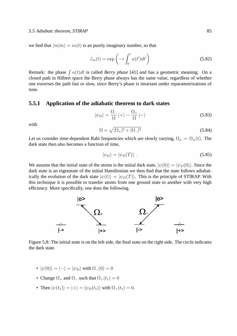
5.5 Adiabatc theorem, STIRAP 85
we find that〈m|m〉 = iα(t) is an purely imaginary number, so that
cm(t) = exp
(−i∫ t
0
α(t′)dt′)
(5.82)
Remark: the phase∫α(t)dt is calledBerry phase[41] and has a geometric meaning. On a
closed path in Hilbert space the Berry phase always has the same value, regardless of whetherone traverses the path fast or slow, since Berry’s phase is invariant under reparametrizations oftime.
5.5.1 Application of the adiabatic theorem to dark states
|ψD〉 =Ω−Ω|+〉 − Ω+
Ω|−〉 (5.83)
withΩ =
√|Ω+|2 + |Ω−|2 (5.84)
Let us consider time-dependent Rabi frequencies which are slowly varying,Ω± = Ω±(t). Thedark state then also becomes a function of time,
|ψD〉 = |ψD(T )〉 . (5.85)
We assume that the initial state of the atoms is the initial dark state,|ψ(0)〉 = |ψD(0)〉. Since thedark state is an eigenstate of the initial Hamiltonian we then find that the state follows adiabat-ically the evolution of the dark state|ψ(t)〉 = |ψD(T )〉. This is the principle of STIRAP. Withthis technique it is possible to transfer atoms from one ground state to another with very highefficiency. More specifically, one does the following.
Figure 5.8: The initial state is on the left side, the final state on the right side. The circle indicatesthe dark state.
• |ψ(0)〉 = |−〉 = |ψD〉 with Ω−(0) = 0
• ChangeΩ+ andΩ− such thatΩ+(t1) = 0
• Then|ψ(t1)〉 = |+〉 = |ψD(t1)〉 with Ω+(t1) = 0.
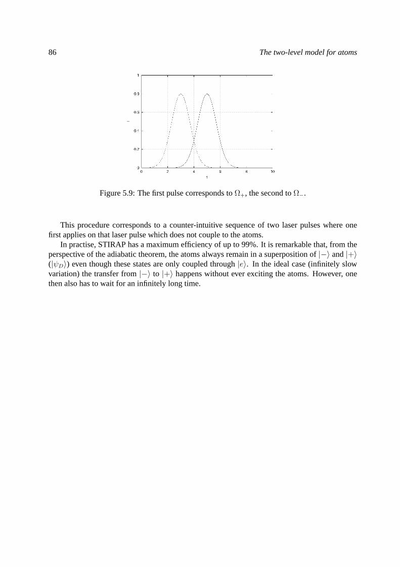
86 The two-level model for atoms
Figure 5.9: The first pulse corresponds toΩ+, the second toΩ−.
This procedure corresponds to a counter-intuitive sequence of two laser pulses where onefirst applies on that laser pulse which does not couple to the atoms.
In practise, STIRAP has a maximum efficiency of up to 99%. It is remarkable that, from theperspective of the adiabatic theorem, the atoms always remain in a superposition of|−〉 and|+〉(|ψD〉) even though these states are only coupled through|e〉. In the ideal case (infinitely slowvariation) the transfer from|−〉 to |+〉 happens without ever exciting the atoms. However, onethen also has to wait for an infinitely long time.
Chapter 6
Atomoptik
Die Atomoptik behandelt allgemein die koharente Propagation atomarer Materiewellen. Haup-taugenmerk wird also auf Schwerpunktbewegung der Atome gelegt. In dieser Vorlesung wirdder Einfluß von Licht auf die Schwerpunktbewegung behandelt.
6.1 Grundlegendes Prinzip
In Kap. 3 behandelten wir, dass der vollstandige atomare Hamiltonian aus Relativ- und Schwer-punktbewegungsbeitragen besteht:
H =p2
2M+∑n
En |n〉 〈n|︸ ︷︷ ︸=H0
(6.1)
wobeiH0 die Relativbewegung der Elektronen berschreibt (|n〉 = 1s, 2p . . .), p der Schwerpunk-timpulsoperator undM die Gesamtmasse des Atoms ist.
Die Kopplung an ein elektromagnetisches Feld ist in der Dipolnaherung nach Abschnitt 4.3gegeben durch:
Hint = − 1
ε0
d ·D(x)− µ ·B(x) (6.2)
Dabei sindd,µ Operatoren, die auf die Relativbewegung wirken,x ist der Schwerpunkt desAtoms. Die Heisenbergschen Bewegungsgleichungen liefern:
x = − i
~[x, H +Hint] =
1
MP (6.3)
P = − i
~[P , Hint] = ∇− 1
ε0
d ·D(x)− µ ·B(x) (6.4)
Inhomogene Felderandern also die Schwerpunktbewegung. Dabei hangt dieAnderung vominneren Zustand ab (z.B. Stern-Gerlach)
88 Atomoptik
Besonders intuitiv zu verstehen ist die Absorption/Emission einzelner Photonen mit Polari-sationεε und Wellenvektork. Der Photonenimpuls ergibt sich zu:
pγ = ~k (6.5)
Aus der Impulserhaltung folgt:
|p, g〉 ⊗ |1k〉 −→ |p + ~k, e〉 ⊗ |0〉 (6.6)
Beispiel: laufende Laser-Welle mit WellenvektorkL
Hint = −d ·E(x) E = E0eikLx (6.7)
Hieraus ergibt sich
Ω = −deg ·E~
= Ω0eikLx (6.8)
Fur ein Zwei”=Niveau”=System gilt dann:
H =p2
2M1 +
(−~∆
0
)+ ~
(0 Ω0e
ikLx
Ω0e−ikLx 0
)(6.9)
Man verwendet folgende Zusammenhange
|ψe〉 =
∫d3p |p〉ψe(p) , analog|ψg〉 (6.10)
mit eikLx |p〉 = |p + ~kL〉 (6.11)
Die letzte Gleichung erhalt man am einfachsten, wenn man die Orstdarstellung der Impulseigen-zustande verwendet:〈x|p〉 ∝ exp(ip · x/~). Man setzt dies in die Schrodinger-Gleichung ein
i~∂t(|ψe〉|ψg〉
)= H
(|ψe〉|ψg〉
)(6.12)
und erhalt:
i~∂t(ψe(p + ~kL)
ψg(p)
)=
( [(p+~kL)2
2M− ~∆
]ψe(p + ~kL) + ~Ω0ψg(p)
p2
2Mψg(p) + ~Ω∗0ψe(p + ~kL)
)(6.13)
Das ist nun wieder ein 2-Niveau-System der Form
(ψe(p + ~kL)
ψg(p)
).
Wichtig: der Impulsubertragandert die Verstimmung:
Ee − Eg =
[(p + ~kL)2
2M− ~∆
]− p2
2M
= −~∆ +~M
p · kL +~2k2
L
2M(6.14)
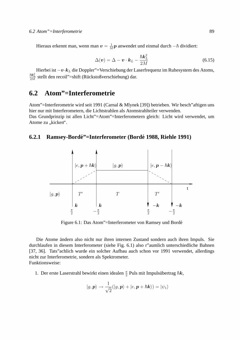
6.2 Atom”=Interferometrie 89
Hieraus erkennt man, wenn manv = 1M
p anwendet und einmal durch−~ dividiert:
∆(v) = ∆− v · kL −~k2
L
2M(6.15)
Hierbei ist−v·kL die Doppler”=Verschiebung der Laserfrequenz im Ruhesystem des Atoms,~k2
L
2Mstellt den recoil”=shift (Ruckstoßverschiebung) dar.
6.2 Atom”=Interferometrie
Atom”=Interferometrie wird seit 1991 (Carnal & Mlynek [39]) betrieben. Wir besch”aftigen unshier nur mit Interferometern, die Lichtstrahlen als Atomstrahlteiler verwenden.Das Grundprinzip ist allen Licht”=Atom”=Interferometern gleich: Licht wird verwendet, umAtome zu
”kicken“.
6.2.1 Ramsey-Borde”=Interferometer (Bord e 1988, Riehle 1991)
T ′t
π2
−k
|e,p + ~k〉 |e,p− ~k〉
T ′
−π2
π2
k
|g,p〉
−k
T
k−π
2
|g,p〉
Figure 6.1: Das Atom”=Interferometer von Ramsey und Borde
Die Atome andern also nicht nur ihren internen Zustand sondern auch ihren Impuls. Siedurchlaufen in diesem Interferometer (siehe Fig. 6.1) also r”aumlich unterschiedliche Bahnen[37, 36]. Tats”achlich wurde ein solcher Aufbau auch schon vor 1991 verwendet, allerdingsnicht zur Interferometrie, sondern als Spektrometer.Funktionsweise:
1. Der erste Laserstrahl bewirkt einen idealenπ2
Puls mit Impulsubertrag~k,
|g,p〉 → 1√2(|g,p〉+ |e,p + ~k〉) = |ψ1〉
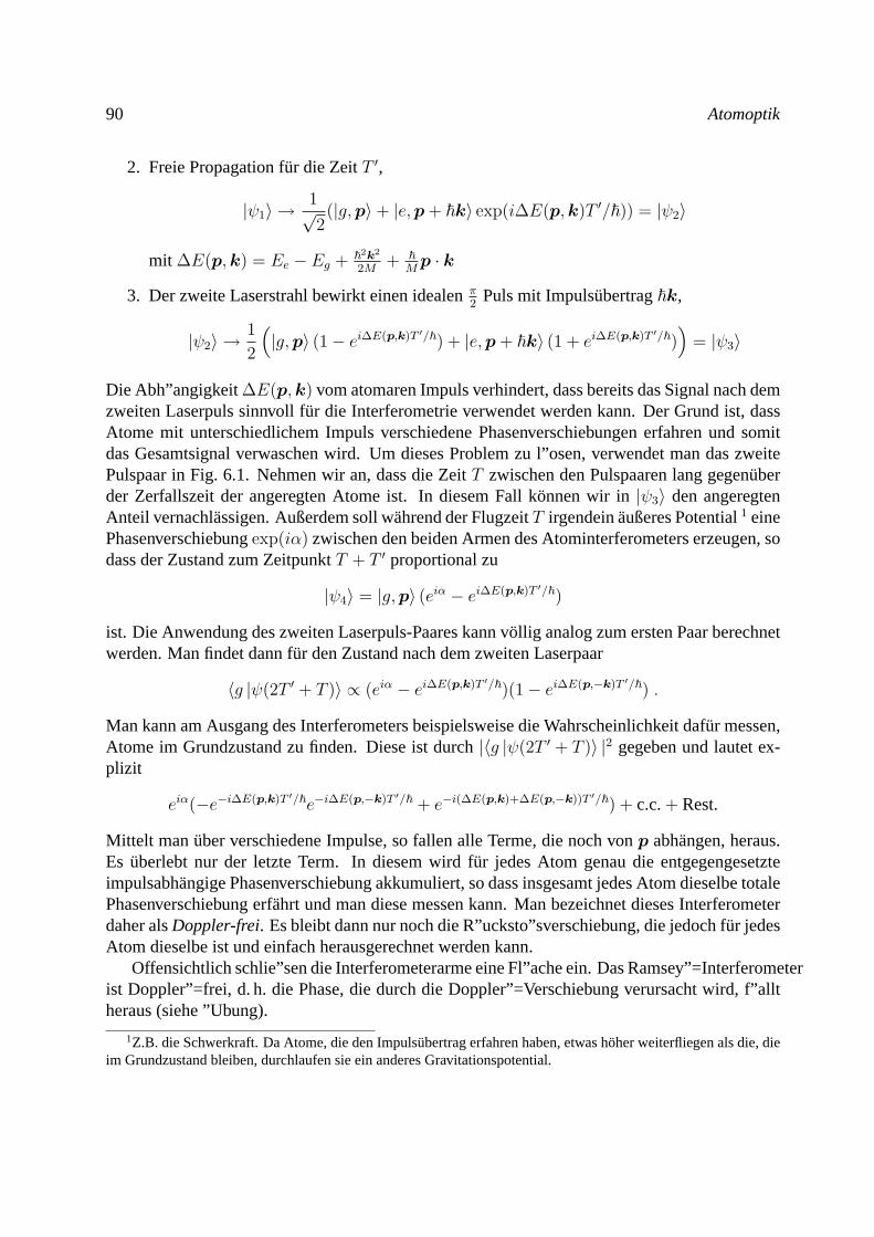
90 Atomoptik
2. Freie Propagation fur die ZeitT ′,
|ψ1〉 →1√2(|g,p〉+ |e,p + ~k〉 exp(i∆E(p,k)T ′/~)) = |ψ2〉
mit ∆E(p,k) = Ee − Eg + ~2k2
2M+ ~
Mp · k
3. Der zweite Laserstrahl bewirkt einen idealenπ2
Puls mit Impulsubertrag~k,
|ψ2〉 →1
2
(|g,p〉 (1− ei∆E(p,k)T ′/~) + |e,p + ~k〉 (1 + ei∆E(p,k)T ′/~)
)= |ψ3〉
Die Abh”angigkeit∆E(p,k) vom atomaren Impuls verhindert, dass bereits das Signal nach demzweiten Laserpuls sinnvoll fur die Interferometrie verwendet werden kann. Der Grund ist, dassAtome mit unterschiedlichem Impuls verschiedene Phasenverschiebungen erfahren und somitdas Gesamtsignal verwaschen wird. Um dieses Problem zu l”osen, verwendet man das zweitePulspaar in Fig. 6.1. Nehmen wir an, dass die ZeitT zwischen den Pulspaaren lang gegenuberder Zerfallszeit der angeregten Atome ist. In diesem Fall konnen wir in|ψ3〉 den angeregtenAnteil vernachlassigen. Außerdem soll wahrend der FlugzeitT irgendeinaußeres Potential1 einePhasenverschiebungexp(iα) zwischen den beiden Armen des Atominterferometers erzeugen, sodass der Zustand zum ZeitpunktT + T ′ proportional zu
|ψ4〉 = |g,p〉 (eiα − ei∆E(p,k)T ′/~)
ist. Die Anwendung des zweiten Laserpuls-Paares kann vollig analog zum ersten Paar berechnetwerden. Man findet dann fur den Zustand nach dem zweiten Laserpaar
〈g |ψ(2T ′ + T )〉 ∝ (eiα − ei∆E(p,k)T ′/~)(1− ei∆E(p,−k)T ′/~) .
Man kann am Ausgang des Interferometers beispielsweise die Wahrscheinlichkeit dafur messen,Atome im Grundzustand zu finden. Diese ist durch|〈g |ψ(2T ′ + T )〉 |2 gegeben und lautet ex-plizit
eiα(−e−i∆E(p,k)T ′/~e−i∆E(p,−k)T ′/~ + e−i(∆E(p,k)+∆E(p,−k))T ′/~) + c.c.+ Rest.
Mittelt manuber verschiedene Impulse, so fallen alle Terme, die noch vonp abhangen, heraus.Es uberlebt nur der letzte Term. In diesem wird fur jedes Atom genau die entgegengesetzteimpulsabhangige Phasenverschiebung akkumuliert, so dass insgesamt jedes Atom dieselbe totalePhasenverschiebung erfahrt und man diese messen kann. Man bezeichnet dieses Interferometerdaher alsDoppler-frei. Es bleibt dann nur noch die R”ucksto”sverschiebung, die jedoch fur jedesAtom dieselbe ist und einfach herausgerechnet werden kann.
Offensichtlich schlie”sen die Interferometerarme eine Fl”ache ein. Das Ramsey”=Interferometerist Doppler”=frei, d. h. die Phase, die durch die Doppler”=Verschiebung verursacht wird, f”alltheraus (siehe ”Ubung).
1Z.B. die Schwerkraft. Da Atome, die den Impulsubertrag erfahren haben, etwas hoher weiterfliegen als die, dieim Grundzustand bleiben, durchlaufen sie ein anderes Gravitationspotential.
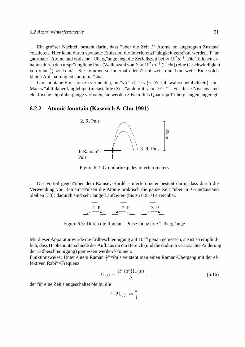
6.2 Atom”=Interferometrie 91
Ein gro”ser Nachteil besteht darin, dass ”uber die ZeitT ′ Atome im angeregten Zustandexistieren. Hier kann durch spontane Emission die Interferenzf”ahigkeit zerst”ort werden. F”ur
”normale“ Atome und optische ”Uberg”ange liegt die Zerfallszeit bei≈ 107 s−1. Die Teilchen er-
halten durch den urspr”ungliche Puls (Wellenzahl vonk ≈ 107 m−1 (Licht)) eine Geschwindigkeitvon v = ~k
M≈ 1 cm/s. Sie kommen so innerhalb der Zerfallszeit rund1 nm weit. Eine solch
kleine Aufspaltung ist kaum me”sbar.Um spontane Emission zu vermeiden, mu”sT ′ 1/γ (γ: Zerfallswahrscheinlichkeit) sein.
Man w”ahlt daher langlebige (metastabile) Zust”ande mitγ ≈ 103 s−1. Fur diese Niveaus sindelektrische Dipolubergange verboten, sie werden z.B. mittels Quadrupol”uberg”angen angeregt.
6.2.2 Atomic fountain (Kasevich & Chu 1991)
1. Raman”=Puls
2. R. Puls
3. R. Puls
20cm
Figure 6.2: Grundprinzip des Interferometers
Der Vorteil gegen”uber dem Ramsey-Borde”=Interferometer besteht darin, dass durch dieVerwendung von Raman”=Pulsen die Atome praktisch die ganze Zeit ”uber im Grundzustandbleiben [38]: dadurch sind sehr lange Laufzeiten (bis zu0.25 s) erreichbar.
1. P. 2. P. 3. P.
Figure 6.3: Durch die Raman”=Pulse induzierte ”Uberg”ange
Mit dieser Apparatur wurde die Erdbeschleunigung auf10−8 genau gemessen, sie ist so empfind-lich, dass H”ohenunterschiede des Aufbaus im cm Bereich (und die dadurch verursachteAnderungder Erdbeschleunigung) gemessen werden k”onnen.Funktionsweise: Unter einem Ramanπ
2”=Puls versteht man einen Raman-Ubergang mit der ef-
fektiven Rabi”=Frequenz
Ωeff =Ω∗+(x)Ω−(x)
∆, (6.16)
der fur eine Zeitt angeschaltet bleibt, die
t · |Ωeff | ≈π
4
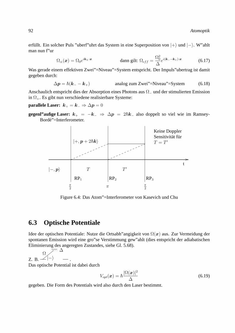
92 Atomoptik
erfullt. Ein solcher Puls ”uberf”uhrt das System in eine Superposition von|+〉 und |−〉. W”ahltman nun f”ur
Ω±(x) = Ω0eik±·x dann gilt:Ωeff =
Ω20
∆ei(k−−k+)·x (6.17)
Was gerade einem effektiven Zwei”=Niveau”=System entspricht. Der Impuls”ubertrag ist damitgegeben durch:
∆p = ~(k− − k+) analog zum Zwei”=Niveau”=System (6.18)
Anschaulich entspricht dies der Absorption eines Photons ausΩ− und der stimulierten Emissionin Ω+. Es gibt nun verschiedene realisierbare Systeme:
parallele Laser: k+ = k− ⇒ ∆p = 0
gegenl”aufige Laser: k+ = −k− ⇒ ∆p = 2~k− also doppelt so viel wie im Ramsey-Borde”=Interferometer.
t
π2
|+,p + 2~k〉
π2
π
|−,p〉 T ′T
RP1 RP2 RP3
Keine DopplerSensitivitat furT = T ′
Figure 6.4: Das Atom”=Interferometer von Kasevich und Chu
6.3 Optische Potentiale
Idee der optischen Potentiale: Nutze die Ortsabh”angigkeit vonΩ(x) aus. Zur Vermeidung derspontanen Emission wird eine gro”se Verstimmung gew”ahlt (dies entspricht der adiabatischenEliminierung des angeregten Zustandes, siehe Gl. 5.68).
Z. B.
∆Ω|−〉 .
Das optische Potential ist dabei durch
Vopt(x) = ~|Ω(x)|2
∆(6.19)
gegeben. Die Form des Potentials wird also durch den Laser bestimmt.
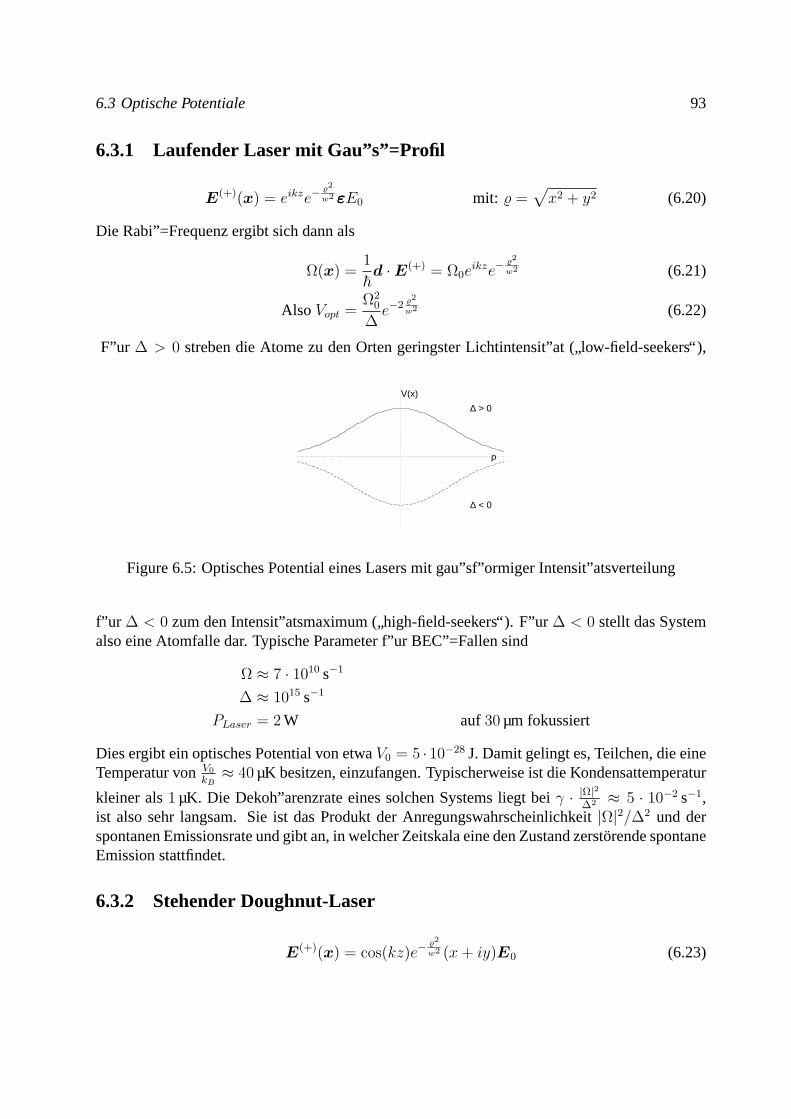
6.3 Optische Potentiale 93
6.3.1 Laufender Laser mit Gau”s”=Profil
E(+)(x) = eikze−%2
w2 εεE0 mit: % =√x2 + y2 (6.20)
Die Rabi”=Frequenz ergibt sich dann als
Ω(x) =1
~d ·E(+) = Ω0e
ikze−%2
w2 (6.21)
Also Vopt =Ω2
0
∆e−2 %2
w2 (6.22)
F”ur ∆ > 0 streben die Atome zu den Orten geringster Lichtintensit”at (”low-field-seekers“),
V(x)
ρ
∆ > 0
∆ < 0
Figure 6.5: Optisches Potential eines Lasers mit gau”sf”ormiger Intensit”atsverteilung
f”ur ∆ < 0 zum den Intensit”atsmaximum (”high-field-seekers“). F”ur∆ < 0 stellt das System
also eine Atomfalle dar. Typische Parameter f”ur BEC”=Fallen sind
Ω ≈ 7 · 1010 s−1
∆ ≈ 1015 s−1
PLaser = 2 W auf30 µm fokussiert
Dies ergibt ein optisches Potential von etwaV0 = 5 · 10−28 J. Damit gelingt es, Teilchen, die eineTemperatur vonV0
kB≈ 40 µK besitzen, einzufangen. Typischerweise ist die Kondensattemperatur
kleiner als1 µK. Die Dekoh”arenzrate eines solchen Systems liegt beiγ · |Ω|2
∆2 ≈ 5 · 10−2 s−1,ist also sehr langsam. Sie ist das Produkt der Anregungswahrscheinlichkeit|Ω|2/∆2 und derspontanen Emissionsrate und gibt an, in welcher Zeitskala eine den Zustand zerstorende spontaneEmission stattfindet.
6.3.2 Stehender Doughnut-Laser
E(+)(x) = cos(kz)e−%2
w2 (x+ iy)E0 (6.23)
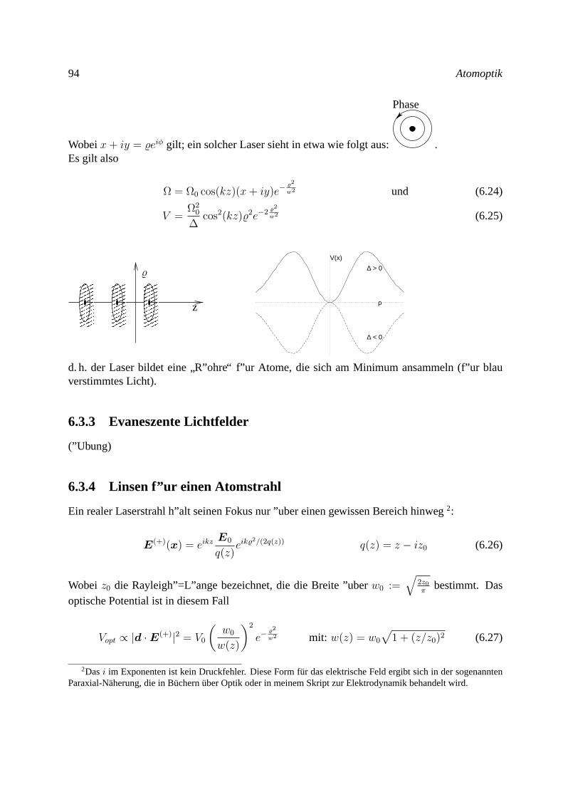
94 Atomoptik
Wobeix+ iy = %eiφ gilt; ein solcher Laser sieht in etwa wie folgt aus:
Phase
.Es gilt also
Ω = Ω0 cos(kz)(x+ iy)e−%2
w2 und (6.24)
V =Ω2
0
∆cos2(kz)%2e−2 %2
w2 (6.25)
%
z
V(x)
ρ
∆ > 0
∆ < 0
d. h. der Laser bildet eine”R”ohre“ f”ur Atome, die sich am Minimum ansammeln (f”ur blau
verstimmtes Licht).
6.3.3 Evaneszente Lichtfelder
(”Ubung)
6.3.4 Linsen f”ur einen Atomstrahl
Ein realer Laserstrahl h”alt seinen Fokus nur ”uber einen gewissen Bereich hinweg2:
E(+)(x) = eikzE0
q(z)eik%
2/(2q(z)) q(z) = z − iz0 (6.26)
Wobei z0 die Rayleigh”=L”ange bezeichnet, die die Breite ”uberw0 :=√
2z0π
bestimmt. Dasoptische Potential ist in diesem Fall
Vopt ∝ |d ·E(+)|2 = V0
(w0
w(z)
)2
e−%2
w2 mit: w(z) = w0
√1 + (z/z0)2 (6.27)
2Dasi im Exponenten ist kein Druckfehler. Diese Form fur das elektrische Feld ergibt sich in der sogenanntenParaxial-Naherung, die in Buchernuber Optik oder in meinem Skript zur Elektrodynamik behandelt wird.
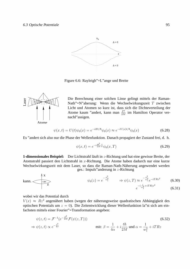
6.3 Optische Potentiale 95
V0
z
∆ > 0
∆ < 0
Figure 6.6: Rayleigh”=L”ange und Breite
Atome
Las
er Die Berechnung einer solchen Linse gelingt mittels der Raman-Nath”=N”aherung: Wenn die WechselwirkungszeitT zwischenLicht und Atomen so kurz ist, dass sich die Dichteverteilung derAtome kaum ”andert, kann manP
2
2Mim Hamilton Operator ver-
nachl”assigen.
ψ(x, t) = U(t)ψ0(x) = e−iHt/~ψ0(x) ≈ e−iV (x)t/~ψ0(x) (6.28)
Es ”andert sich also nur die Phase der Wellenfunktion. Danach propagiert der Zustand frei, d. h.
ψ(x, t) = e−ip2
2Mt~ψ0(x, T ) (6.29)
1-dimensionales Beispiel: Der Lichtstrahl lauft inz-Richtung und hat eine gewisse Breite, derAtomstrahl passiert den Lichtstrahl inx-Richtung. Die Atome haben dadurch nur eine kurzeWechselwirkungszeit mit dem Laser, so dass die Raman-Nath-Naherung angewendet werden
kann.
x
z
ges.: Impuls”anderung inz-Richtung
ψ0(z) = e− z2
w21 ⇒ ψ(z, T ) ≈ e
− z2
w21 e−iTRz
2
(6.30)
e−( 1
w21
+iTR)z2
(6.31)
wobei wir das Potential durchV (x) ≈ Rz2 angenahert haben (wegen der naherungsweise quadratischen Abhangigkeit desoptischen Potentials umz = 0). Die Zeitentwicklung dieser Wellenfunktion la”st sich am ein-fachsten mittels einer Fourier”=Transformation angeben:
ψ(z, t) = F−1(e−p2
2MF(ψ(z, T ))) (6.32)
⇒ ψ(z, t) ∝ e−z2
4β mit: β =1
4α+ i
t~2M
undα =1
w21
+ iTRz
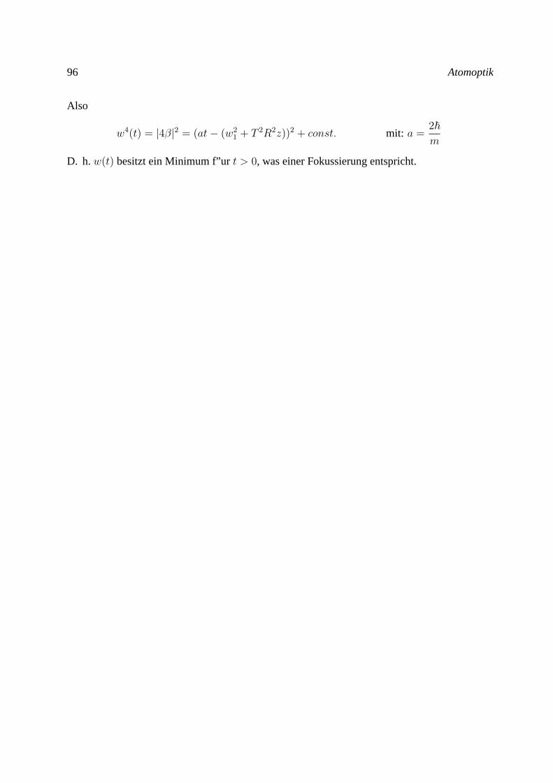
96 Atomoptik
Also
w4(t) = |4β|2 = (at− (w21 + T 2R2z))2 + const. mit: a =
2~m
D. h.w(t) besitzt ein Minimum f”urt > 0, was einer Fokussierung entspricht.
Chapter 7
Incoherent Interaction and Density Matrix
7.1 Density Matrix Formalism
The density matrix% allows us to describe the time evolution of incoherent systems (opposed topure quantum states). In particular, it also makes it possible to describe open quantum systems.An example: A (classical) apparatus in a laboratory produces a quantum state, but only with acertainclassicalprobability. Each time the experiment is performed, the apparatus may producea different state with a certain probability. This could for instance be an oven which produces anatom beam sometimes with velocityv1 and sometimes withv2.One therefore only knows with some probabilitypi, i = 1, 2, . . . whether a state|ψi〉 has beenprepared. The states|ψi〉 need not to be orthogonal. Of course the classical probabilities mustfullfill
∑i pi = 1, sincesomestate has been prepared with certainty. In a closed quantum
system (not coupled to a reservoir), each state|ψi〉 then evolves unitarily according to|ψi(t)〉 =
e−i~Ht |ψi(0)〉. If in one run of the experiment the state|ψi〉 has been prepared, the expectation
value of any observable for this state is given by
〈A〉i = 〈ψi(t)|a|ψi(t)〉 (7.1)
In each run of the experiment, the state|ψi〉 is prepared with probabilitypi. One can calculatethe full expectation value by averaging over all states which can be prepared,
〈A〉 =∑i
pi 〈A〉i =∑i
pi 〈ψi(t)|a|ψi(t)〉 (7.2)
If |n〉 is an orthonormal basis of Hilbert space, one can write the identity operator 1as∑n |n〉〈n|. We therefore find for the expectation value
〈A〉 =∑i
pi 〈ψi|∑n
|n〉 〈n|A|ψi〉 =∑n
〈n|A∑i
pi|ψi〉 〈ψi|n〉 =∑n
〈n|A%|n〉 (7.3)
TheDensity matrix% is defined by
% =∑i
pi |ψi〉〈ψi| (7.4)
98 Incoherent Interaction and Density Matrix
The expectation value of an operator then can be expressed as a trace over the operator and thedensity matrix,
〈A〉 = Tr (%A) (7.5)
Properties of the trace
(i) The trace does not depend on the choice of basis.
(ii) Tr (AB) = Tr (BA)
Proof:
ad (i) Let |n′〉 be another basis of Hilbert space. Then
Tr (A) =∑n
〈n|A|n〉 =∑n
〈n|∑n′
|n′〉 〈n′|A|n〉
=∑n′
〈n′| A∑n
|n〉〈n|︸ ︷︷ ︸1
n′〉 =∑n′
〈n′|A|n′〉
ad (ii)
Tr (AB) =∑n
〈n|AB|n〉 =∑n,n′
〈n|A|n′〉 〈n′|B|n〉
=∑n,n′
〈n′|B|n〉 〈n|A|n′〉 =∑n′
〈n′|BA|n′〉
Properties of the density matrix
(i) % is Hermitean.
(ii) Tr % = 1
(iii) Tr (%2) ≤ 1 (= 1 for pure states)
Proof:
ad (i) trivial because ofpi ∈ [0, 1]
ad (ii)
Tr % =∑n,i
〈n|pi|ψi〉 〈ψi|n〉 =∑i
pi 〈ψi|∑n
|n〉 〈n|ψi〉
=∑i
pi 〈ψi|ψi〉︸ ︷︷ ︸1
=∑i
pi = 1
7.1 Density Matrix Formalism 99
ad (iii)
Tr (%2) =∑n
〈n|∑ij
pi|ψi〉 〈ψi|pj|ψj〉 〈ψj|n〉 =∑i,j
pipj 〈ψi|ψj〉 〈ψj|ψi〉
=∑i,j
pipj | 〈ψi|ψj〉 |2︸ ︷︷ ︸≤1
≤∑i
pi∑j
pj = 1
For apure stateone has:% = |ψ〉 〈ψ| , %2 = %
A mixturehas at least two different states:
% = p1 |ψ1〉〈ψ1|+ p2 |ψ2〉〈ψ2|+ . . . , pi 6= 0
The physical difference between a mixture of two states and a superposition becomes veryclear by considering the following example: Let%G describe a mixture:
%G =1
2(|e〉〈e|+ |g〉〈g|)
Half of the atoms are excited, and half are in the ground state. Let us calculate the expectationvalue of the dipole operator,d ∝ |e〉〈g|+ |g〉〈e|.
〈d〉 ∝ Tr (%G(|e〉〈g|+ |g〉〈e|)) =1
2Tr (|g〉〈e|+ |e〉〈g|)
=1
2〈e| . . . |e〉+
1
2〈g| . . . |g〉 = 0
Let %S describe the following superposition,
|ψ〉 =1√2(|e〉+ |g〉)
%S = |ψ〉〈ψ| = 1
2(|e〉+ |g〉)(〈g|+ |e〉)
=1
2(|g〉〈g|+ |e〉〈e|)︸ ︷︷ ︸b%G
+1
2(|e〉〈g|+ |g〉〈e|)
%S has non-diagonal matrix elements, which are calledcoherences. The expectation value of thedipole operator is given by
〈d〉 ∝ Tr (%S(|e〉〈g|+ |g〉〈e|)) = Tr ((%G +1
2(|e〉〈g|+ |g〉〈e|))(|e〉〈g|+ |g〉〈e|))
= 0 +1
2Tr (|e〉〈e|+ |g〉〈g|︸ ︷︷ ︸
1
) = 1
The non-diagonal elements of the density matrix describe the degree of quantum mechanicalcoherence of the system, i.e., its ability to show intertference effects. This is the reason why theyare called coherences. The diagonal elements are equaivalent to the population of each state.
100 Incoherent Interaction and Density Matrix
7.2 Liouville Equation, Superoperators
We consider the time evolution of% in a closed quantum system. A pure state of course fullfillsthe Schrodinger equation:
i~∂t |ψi〉 = H |ψi〉
This can be used to derive an equation for the density matrix:
i~∂t% = i~∑i
pi∂t(|ψi〉〈ψi|) = i~∑i
pi(∂t |ψi〉 〈ψi|+ |ψi〉 ∂t 〈ψi|)
=∑i
pi(H |ψi〉〈ψi| − |ψi〉〈ψi|H)
i~∂t% = [H, %] (7.6)
This is the Liouville equation for closed systems.The trace of the density matrix is time independent:
i~∂tTr % = Tr ([H, %]) = Tr (H%− %H) = 0
[H, ·] is a special cases of so-called superoperators, which act on operators instead of states.
L% := [H, %]
is calledLiouville”=Superoperator. Let us now solve the Liouville equationi~∂t% = L%. For-mally this is quickly done:
%(t) = e−i~ tL%(0) = (1− i
~tL − t2
2!~2LL+ · · · )%(0)
= %(0)− it
~[H, %(0)]− t2
2!~2[H, [H, %(0)]] + . . . = e−
i~Ht%(0)e
i~Ht
Proof:
f(t) := e−it~ L%(0) → i~∂tf = Lf = [H, f ]
g(t) := e−i~Ht%(0)e
i~Ht
to show:f(t) = g(t)
i~∂tg = i~(− i
~Hg +
i
~gH) = [H, g]
f(t) andg(t) fullfill the same differential equation.
f(0) = %(0) = g(0)
f(t) andg(t) fullfill the same initial conditions.
→f(t) = g(t)
7.2 Liouville Equation, Superoperators 101
Entropy, Equilibrium Density Matrix (This is a short deviation to statistical mechanics)The entropy of a quantum system is defined by
S = −kBTr (% ln %) = −kB 〈ln %〉 (7.7)
S describes the degree of order in a system.In (7.7) we take the logarithm of the density matrix. Generally, a functionf(A) of an operator isdefined by refering to its diagonal representation.
A |an〉 = an |an〉 → A =∑n
an |an〉〈an|
For Hermitean operators we have〈an|am〉 = δnmf should be expandable into a Taylor series,
f(A) =∑l
fll!Al
A2 =∑n
an |an〉〈an|∑m
am |am〉〈am| =∑n
a2n |an〉〈an|
This can be generalized to arbitrary powers:
Al =∑n
aln |an〉〈an|
⇒ f(A) =∑l
fll!
∑n
aln |an〉〈an| =∑n
f(an) |an〉〈an| (7.8)
We can employ this to calculate the entropy of a pure state:
% = 1 · |ψ〉〈ψ|S = −kBTr (% ln %) = −kBTr (1 · |ψ〉〈ψ| · ln(1)︸︷︷︸
=0
|ψ〉〈ψ|)
The entropy of a pure state is 0.For a system in equilibrium we have
˙% = 0 ⇔[H, %
]= 0
⇒ % has the same eigenvectors asH
H |En〉 = En |En〉
⇒ % =∑n
%n |En〉〈En|
Thermal equilibrium: maximise the entropyS under the constraints
102 Incoherent Interaction and Density Matrix
• Tr (%) = 1 (Conservation of total probability )
•⟨H⟩
= E (For canonical or grand canonical ensemble)
To do so we introduce two Lagrange parametersλ1, λ2. Maximising results in
∂
∂%n
(S − λ1(Tr (%)− 1)− λ2(
⟨H⟩− E
)= 0
Since% is diagonal in this basis we find
∂
∂%n
−kB
∑n′
%n′ ln %n′ − λ1
(∑n′
%n′ − 1
)− λ2
(∑n′
%n′En′ − E
)= 0
⇒ 0 = −kB (ln %n + 1)− λ1 − λ2En
⇒ %n = exp
− 1
kB(λ1 + λ2En)
∼ e
− λ2kB
En
λ1 is fixed by∑
n %n = 1
⇒ % ∼∑n
e− λ2
kBEn |En〉〈En|
Consider this as a function ofH% ∼ e
− λ2kB
H
Let λ2 = 1T⇒ % = 1
Ze−βH , β = 1
kBT, Z = Tr
(e−βH
)Liouville’s Theorem The entropy of a system is not changed if a unitary transformation isapplied to the density matrix operator.
%′ = U%U †
S ′ = −kBTr (%′ ln %′) = S(%′) = S(U%U †
)Taylor expansion of the operator inside the trace:
K(%′) := %′ ln %′ =∑n
Kn%′n =
∑n
Kn
(U%U †
)nEvaluate the term in parentheses,(
U%U †)n
= U%U †U︸︷︷︸1
%U †U%U † . . .
= U%nU †
7.3 Reduced density matrix, Zwanzig’s Master Equation 103
⇒ K(%′) = U∑
Kn%nU †
⇒ S ′ = −kBTr(U% ln %U †
)= −kBTr
(U †U% ln %
)= S
⇒ The entropy cannot be changed by the time evolutionU = exp(−iHt/~) in a closedsystem. If one wants to change it, the quantum system must be open. This means that the systemcan exchange energy, momentum, or particles by a coupling to the environment or reservoir. Thisis exploited in cooling of quantum systems.
7.3 Reduced density matrix, Zwanzig’s Master Equation
Direct product of Hilbert spaces Consider two Hilbert spacesHS, HR with bases|Sn〉,|Rα〉. Their direct product is given by
HS ⊗HR =
|ψ〉
∣∣∣∣∣|ψ〉 =∑n,α
ψnα |Sn〉 ⊗ |Rα〉
This space does not only contain product states of the form|Sn〉⊗|Rα〉, but alsoentangled states,z.B.
|S1〉 ⊗ |R1〉+ |S2〉 ⊗ |R2〉
Entangled states play a very important role in many modern areas of Physics (Quantum informa-tion, Bell inequalities, Quantum computing, ..). They are special with respect to the correlationsbetween the two subsystemsR andS. Correlations in entangled states cannot be explained byany cassical model. More on this topic can be found in Ref. [19].
Let % be the density matrix in the spaceHS ⊗HR. The expectation value of operators which
only act on states inHS is given by⟨AS
⟩= Tr
(%(AS ⊗ 1R
)). Here, the operatorAS acts
only onHS:AS : HS → HS : |Sn〉 7→ AS |Sn〉
AS ⊗ 1R is the representation of this operator on the product Hilbert space. It acts like
AS ⊗ 1R : HS ⊗HR → HS ⊗HR
|Sn〉 ⊗ |Rα〉 7→ AS |Sn〉 ⊗ 1R |Rα〉
7.3.1 Reduced Density Matrix, Projection Superoperators
The trace of an operator in product space can therefore be decomposed as
Tr (O)HS⊗HR=∑n,α
(〈Sn| ⊗ 〈Rα|) O (|Sn〉 ⊗ |Rα〉)
104 Incoherent Interaction and Density Matrix
⇒ ⟨AS
⟩=∑n,α
〈Sn| ⊗ 〈Rα| %(AS ⊗ 1R) |Sn〉 ⊗ |Rα〉
=∑n
〈Sn|∑α
〈Rα| % |Rα〉 AS |Sn〉
=∑n
〈Sn|TrR (%)AS |Sn〉
In the last step we have used that the operator acts only on one subspace.
TrR (%) ≡∑α
〈Rα| % |Rα〉
Define%S = TrR (%)
reduced density matrix.%S act onHS. In particular we have⟨
AS
⟩= TrS (%SAS) = TrS (TrR (%)AS))
Obviously, the reduced density matrix contains the full information about the expectation valuesof all observables on the system Hilbert spaceHS.
Aim: Find an equation for the evolution of%S alone.
Projection Superoperators In quantum mechanics, ordinary projection operatorsP , like P =|e〉〈e| with P |ψ〉 = |e〉 〈e|ψ〉, fullfill P 2 = P , P † = P
Analogously we find for the action of a projection superoperator on an operator
P2A = PA
Examples:
1. Reduced density matrix
P % ≡ %R(0)TrR (%) , (7.9)
where%R(0) corresponds to the density matrix of the reservoir at timet = 0
P2% = %R(0)TrR (P %)= %R(0)TrR (%R(0) TrR (%)︸ ︷︷ ︸
%S :HS 7→HS
)
⇒P2% = %R(0)TrR (%R(0)) %S = P %
7.3 Reduced density matrix, Zwanzig’s Master Equation 105
2. Projection on the populations
P % ≡∑n
|n〉 〈n| % |n〉 〈n|
P projects% on its diagonal elements, i.e., all coherences are removed.
7.3.2 Zwanzig’s Master Equation
Zwanzig’s Master equation is an equation forP % alone, which is derived from Liouville’s equa-tion
i~% = L%
for %. To do so we first introduce a second projection superoperatorQ := 1− P, which fullfillsQ2 = Q.1 The projection superoperator is time-independent,P = 0,
⇒ i~∂
∂tP% = PL% = PL(P +Q)%
⇒ i~∂
∂tP% = PLP%+ PLQ%
analogously withQ%
i~∂
∂tQ% = QLP%+QLQ% (7.10)
First we solvei~Q% = QLQ%. When the superoperators are time-independent, the formalsolution is easyly given:
Q%(t) = exp(−iQLQt/~)Q%(0) .
The general case is considerably more complicated and leads to a so-called time-ordered expo-nential. Since this appearsveryoften in the interaction picture and in quantum field theory, wewillconsider this in more detail here.
The Time-Ordered Exponential
Formal solution:
i~∫ t
0
Q%dt =
∫ t
0
QL(t′)Q%(t′)dt′ (7.11)
⇒ Q%(t) = Q%(0)− i
~
∫ t
0
QL(t′)QQ%(t′)dt′ (7.12)
1There is an important difference between projection operators and projection superoperators. For projection
operators one has|ψ〉 =(P |ψ〉Q |ψ〉
). However, for superoperators we haveA =
(PAP PAQQAP QAQ
)
106 Incoherent Interaction and Density Matrix
where in the last step we usedQ2 = Q. This solution is only formal since it contains itself:Q%(t) depends onQ%(t′) with t′ < t. If Q%(t′) is rewritten using again Eq. (7.12), one arrives at
Q%(t) = Q%(0)− i
~
∫ t
0
dt′(QL(t′)Q)Q%(0)− i
~
∫ t′
0
dt′′QL(t′′)QQ%(t′′) (7.13)
Iteration leads to
⇒ Q%(t) = Q%(0)− i
~
∫ t
0
dt′(QL(t′)Q)Q%(0)
+
(− i
~
)2 ∫ t
0
dt′∫ t′
0
dt′′(QLQ(t′))(QLQ(t′′))Q%(0) + . . . (7.14)
We introduce thetime-ordered product:
T (A(t)B(t′)) :=
A(t)B(t′) for t > t′
B(t′)A(t) for t′ > t(7.15)
This allows us to rewrite the multiple integrals in the series in the following way:∫ t
0
dt1QLQ(t1)
∫ t1
0
dt2QLQ(t2) =
∫ t
0
dt2
∫ t
t2
dt1T (QLQ(t1) QLQ(t2)) (7.16)
T (QLQ(t1) QLQ(t2)) has also the correct ordering of the operators (the operator at a later timeis to the left of that at an earlier time) ift1 < t2. Consider therefore the following integral withmodified boundary values fort2:
⇒∫ t
0
dt1
∫ t
0
dt2T (QLQ(t1) QLQ(t2))
=
∫ t
0
dt1
∫ t1
0
dt2QLQ(t1) QLQ(t2) +
∫ t
0
dt1
∫ t
t1
dt2QLQ(t2) QLQ(t1) (7.17)
The first term on the right-hand side (rhs) of Eq. (7.17) appears in the series (Eq. (7.14)) vor. Thesecond term on the rhs of Seite von Eq. (7.17) can be written as∫ t
0
dt1
∫ t
t1
dt2QLQ(t2) QLQ(t1) =
∫ t
0
dt2
∫ t2
0
dt1QLQ(t2) QLQ(t1) . (7.18)
With t′1 = t2 undt′2 = t1 it follows that
⇒ 2ndTerm in Eq. (7.17)=∫ t
0
dt′1
∫ t′1
0
dt′2QLQ(t′1) QLQ(t′2) (7.19)
Eq. (7.19) is again a term which appears in the series Reihe (Eq. (7.14)).
⇒∫ t
0
dt1
∫ t1
0
dt2QLQ(t1) QLQ(t2)
=1
2!
∫ t
0
dt1
∫ t
0
dt2T (QLQ(t1) QLQ(t2)) (7.20)
7.3 Reduced density matrix, Zwanzig’s Master Equation 107
We thus have found an expression for the first term in the series in which the integrals haveindependent boundaries. It can be shown that generally∫ t
0
dt1
∫ t1
0
dt2 . . .∫ tn−1
0
dtnQLQ(t1) . . .QLQ(tn)
=1
n!
∫ t
0
dt1 . . .∫ t
0
dtnT (QLQ(t1) . . .QLQ(tn)) (7.21)
⇒ Q%(t) = 1− i
~
∫ t
0
dt1QLQ . . .
+1
n!
(−i~
)n ∫ t
0
dt1 . . .∫ t
0
dtnT (QLQ(t1) . . .QLQ(tn)Q%(0)
= T exp
(−i~
∫ t
0
dt′QLQ(t′)
)Q%(0) (7.22)
= : UQQ(t)Q%(0) (7.23)
This is the solution of the homgeneous differential equation
i~Q% = QLQ(Q%) (7.24)
The time-ordered exponentialT exp is defined by its Taylor series, in which integrals over dif-ferent variablest1, t2, . . . do appear. The time-ordering operatorT guarantees that the operatorsappear in the same order as in the series (7.14) erscheinen.
Derivation of Master equation continued
To derive the Master equation it is now useful to make the ansatzQ%(t) = UQQ(t)%Q(t) .
⇒ i~∂tQ% = i~UQQ%Q + i~UQQ ˙%Q (7.25)
With UQQ = − i~QLQ(t)UQQ(t) and using Eq. (7.10) we find
i~ ˙%Q = U−1QQ(t)QLP%(t) (7.26)
⇒ %Q(t) = %Q(0)− i
~
∫ t
0
dt′U−1QQ(t′)QLP%(t′) (7.27)
⇒ Q%(t) = Q%(0)− i
~UQQ(t)
∫ t
0
dt′U−1QQ(t′)QLQP%(t′) (7.28)
Insert Eq. (7.28) into the equation forP%:
i~P % = PLP%+ PL(t)QQ%(0)− i
~UQQ(t)
∫ t
0
dt′U−1QQ(t′)QLP%(t′)
(7.29)
108 Incoherent Interaction and Density Matrix
Eq. (7.29) isZwanzig’s Master equation.This is a exact differential equation forP% alone, but it generally cannot be solved withoutapproximations. To simplify it we now consider the special case of a projetion superoperator ofthe form 7.9 with the following features:
1. %(0) = %R(0) ⊗ %S(0), i.e., there are no correlation between the system and the reservoirat timet = 0
2. [%R(0), HR] = 0, i.e., the reservoir is in a stationary state ofHR (we setH = HR +HS +Hint).
3. Tr R(%R(0)Hint) = 0 e.g. Hint = −d · E, here the reservoir corresponds to the radiationfield⇒ TrR (%R(0)Hint) = −d 〈E〉 (t = 0) = 0. 2
When these conditions are valid one finds
Q%(0) = %(0)− P%(0)= %R(0)⊗ %S(0)− %R(0)⊗ TrR (%R(0)⊗ %S(0))
= %R(0)⊗ %S(0)− %R(0)⊗ %S(0)
= 0 (7.30)
The following relations for an arbitrary operatorX are left to the reader as an excercise:
PLPX = %R(0)[HS,TrR (X)] = PLSX (7.31)
PLQX = %R(0)TrR ([Hint, X]) = PLintX (7.32)
QLPX = [Hint, %R(0)TrR (X)] = LintPX (7.33)
Furthermore,
QLQX = (1− P)LQX= LQX − PLQX= L(1− P)X − PLintX
= LX − LPX − PLintX
= [HS +HR +Hint, X]− [HS +HR +Hint, %R(0)TrR (X)]
−%R(0)TrR ([Hint, X])
= [HS +HR +Hint, X]− [HS, %R(0)TrR (X)]
−[HR, %R(0)]TrR (X)− [Hint, %R(0)TrR (X)]
−%R(0)TrR ([Hint, X])
2In a stationary state in free space one has〈E〉 = 0, since such a state corresponds to a mixture (i.e., nota superposition) of number states. BecauseE ∼ a + a+ one then finds〈n| a + a+ |n〉 = 〈n| (
√n |n− 1〉 +√
n+ 1 |n+ 1〉) = 0
7.3 Reduced density matrix, Zwanzig’s Master Equation 109
Using [HR, %R(0)] = 0 one deduces
QLQX = [HS, X − PX] + [HR, X] + [Hint, X − PX]− P [Hint, X]
= [HS,QX] + LRX + [Hint,QX]− PLintX
= (LSQ+ LR + LintQ−PLint)X (7.34)
Additional properties:
LSQ = QLS (7.35)
PLS = LSP (7.36)
Insertion into the master equation (Eq. (7.29)) results in
i~P % = PLSP%−i
~PLint
∫ t
0
dt′UQQ(t)U−1QQ(t′)LintP%(t′)
UQQ(t) = T exp
(−i~
∫ t
0
dt′′QL(t′′)Q)
L(t)X = [H(t), X] = [HS +HR +Hint, X]
Approximation: take only terms up to 2nd order inHint into acount (assumption:Hint HR, HS)
⇒ UQQ ≈ exp
(− i
~Q(Ls + LR)Qt
)(if HS andHR are time independent).
QLs = LsQ ⇒ QLsQ = LsQ = QLsQLR = LRQ = LR
⇒ UQQ = e−iQLst/~e−iLRt/~
In the last stepLsLR = LRLs was used, which can be proven in the following way:
(LRLs − LsLR)X =[HR, [HS, X]
]−[HS, [HR, X]
]=
[HR, [HS, X]
]+[HS, [X,HR]
]= −
[X, [HR, HS]︸ ︷︷ ︸
=0
]= 0
where Jakobi’s identity was employed. One then finds
e−iQLst/~ =∞∑n=0
(− it/~
)nn!
(QLs
)n(QLs)n = LnsQn = LnsQ n > 0
⇒ e−iQLst/~QLP = e−iLst/~QLP
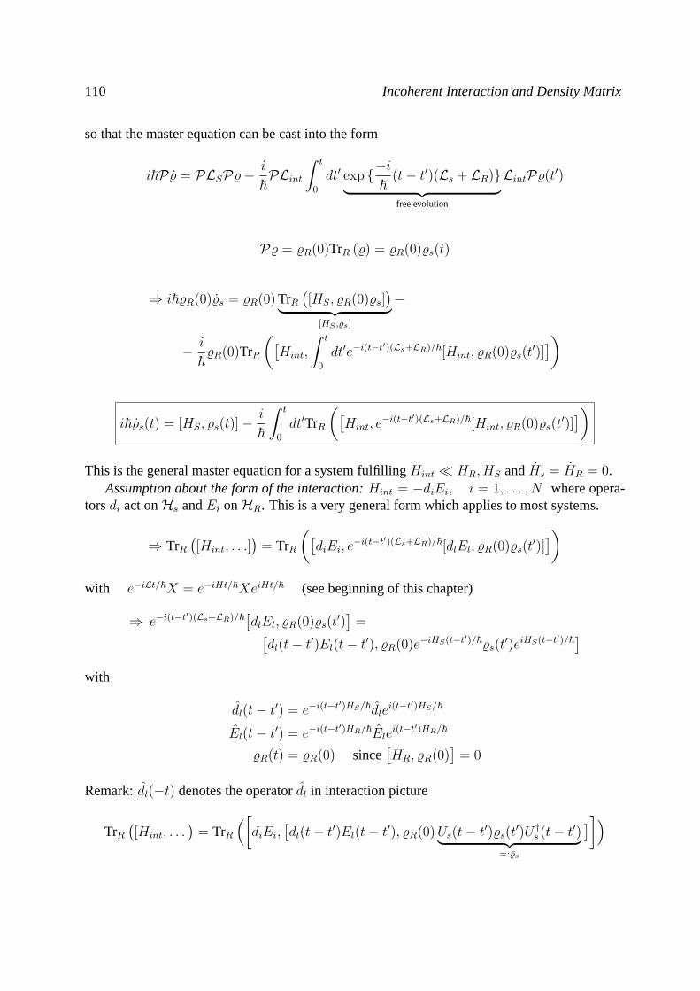
110 Incoherent Interaction and Density Matrix
so that the master equation can be cast into the form
i~P % = PLSP%−i
~PLint
∫ t
0
dt′ exp −i~
(t− t′)(Ls + LR)︸ ︷︷ ︸free evolution
LintP%(t′)
P% = %R(0)TrR (%) = %R(0)%s(t)
⇒ i~%R(0)%s = %R(0) TrR([HS, %R(0)%s]
)︸ ︷︷ ︸[HS ,%s]
−
− i
~%R(0)TrR
([Hint,
∫ t
0
dt′e−i(t−t′)(Ls+LR)/~[Hint, %R(0)%s(t
′)]])
i~%s(t) = [HS, %s(t)]−i
~
∫ t
0
dt′TrR
([Hint, e
−i(t−t′)(Ls+LR)/~[Hint, %R(0)%s(t′)]])
This is the general master equation for a system fulfillingHint HR, HS andHs = HR = 0.Assumption about the form of the interaction:Hint = −diEi, i = 1, . . . , N where opera-
torsdi act onHs andEi onHR. This is a very general form which applies to most systems.
⇒ TrR([Hint, . . .]
)= TrR
([diEi, e
−i(t−t′)(Ls+LR)/~[dlEl, %R(0)%s(t′)]])
with e−iLt/~X = e−iHt/~XeiHt/~ (see beginning of this chapter)
⇒ e−i(t−t′)(Ls+LR)/~[dlEl, %R(0)%s(t
′)]
=[dl(t− t′)El(t− t′), %R(0)e−iHS(t−t′)/~%s(t
′)eiHS(t−t′)/~]with
dl(t− t′) = e−i(t−t′)HS/~dle
i(t−t′)HS/~
El(t− t′) = e−i(t−t′)HR/~Ele
i(t−t′)HR/~
%R(t) = %R(0) since[HR, %R(0)
]= 0
Remark:dl(−t) denotes the operatordl in interaction picture
TrR([Hint, . . .
)= TrR
([diEi,
[dl(t− t′)El(t− t′), %R(0)Us(t− t′)%s(t
′)U †s (t− t′)︸ ︷︷ ︸=:%s
]])
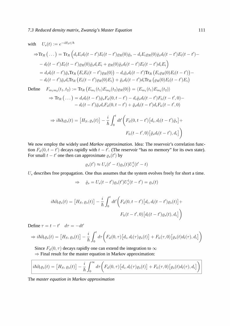
7.3 Reduced density matrix, Zwanzig’s Master Equation 111
with Us(t) := e−iHSt/~
⇒TrR(. . .)
= TrR(diEidl(t− t′)El(t− t′)%R(0)%s − diEi%R(0)%sdl(t− t′)El(t− t′)−
− dl(t− t′)El(t− t′)%R(0)%sdiEi + %R(0)%sdl(t− t′)El(t− t′)diEi
)= didl(t− t′)%sTrR
(EiEl(t− t′)%R(0)
)− di%sdl(t− t′)TrR
(Ei%R(0)El(t− t′)
)−
− dl(t− t′)%sdiTrR(El(t− t′)%R(0)Ei
)+ %sdl(t− t′)diTrR
(%R(0)El(t− t′)Ei
)Define Fm1m2(t1, t2) := TrR
(Em1(t1)Em2(t2)%R(0)
)= 〈Em1(t1)Em2(t2)〉
⇒ TrR(. . .)
= didl(t− t′)%sFil(0, t− t′)− di%sdl(t− t′)Fli(t− t′, 0)−− dl(t− t′)%sdiFil(0, t− t′) + %sdl(t− t′)diFli(t− t′, 0)
⇒ i~∂t%s(t) =[HS, %s(t)
]− i
~
∫ t
0
dt′(Fil(0, t− t′)
[di, dl(t− t′)%s
]+
Fli(t− t′, 0)[%sdl(t− t′), di
])We now employ the widely usedMarkov approximation. Idea: The reservoir’s correlation func-tion Fil(0, t − t′) decays rapidly witht − t′. (The reservoir “has no memory” for its own state).For smallt− t′ one then can approximate%s(t′) by
%s(t′) ≈ Us(t
′ − t)%s(t)U†s (t′ − t)
Us describes free propagation. One thus assumes that the system evolves freely for short a time.
⇒ %s = Us(t− t′)%s(t′)U †s (t− t′) = %s(t)
i~∂t%s(t) =[HS, %s(t)
]− i
~
∫ t
0
dt′(Fil(0, t− t′)
[di, dl(t− t′)%s(t)
]+
Fli(t− t′, 0)[dl(t− t′)%s(t), di
])Defineτ = t− t′ dτ = −dt′
⇒ i~∂t%s(t) =[HS, %s(t)
]− i
~
∫ t
0
dτ
(Fil(0, τ)
[di, dl(τ)%s(t)
]+ Fli(τ, 0)
[%s(t)dl(τ), di
])SinceFil(0, τ) decays rapidly one can extend the integration to∞⇒ Final result for the master equation in Markov approximation:
i~∂t%s(t) =[HS, %s(t)
]− i
~
∫ ∞0
dτ
(Fil(0, τ)
[di, dl(τ)%s(t)
]+ Fli(τ, 0)
[%s(t)dl(τ), di
])Themaster equation in Markov approximation
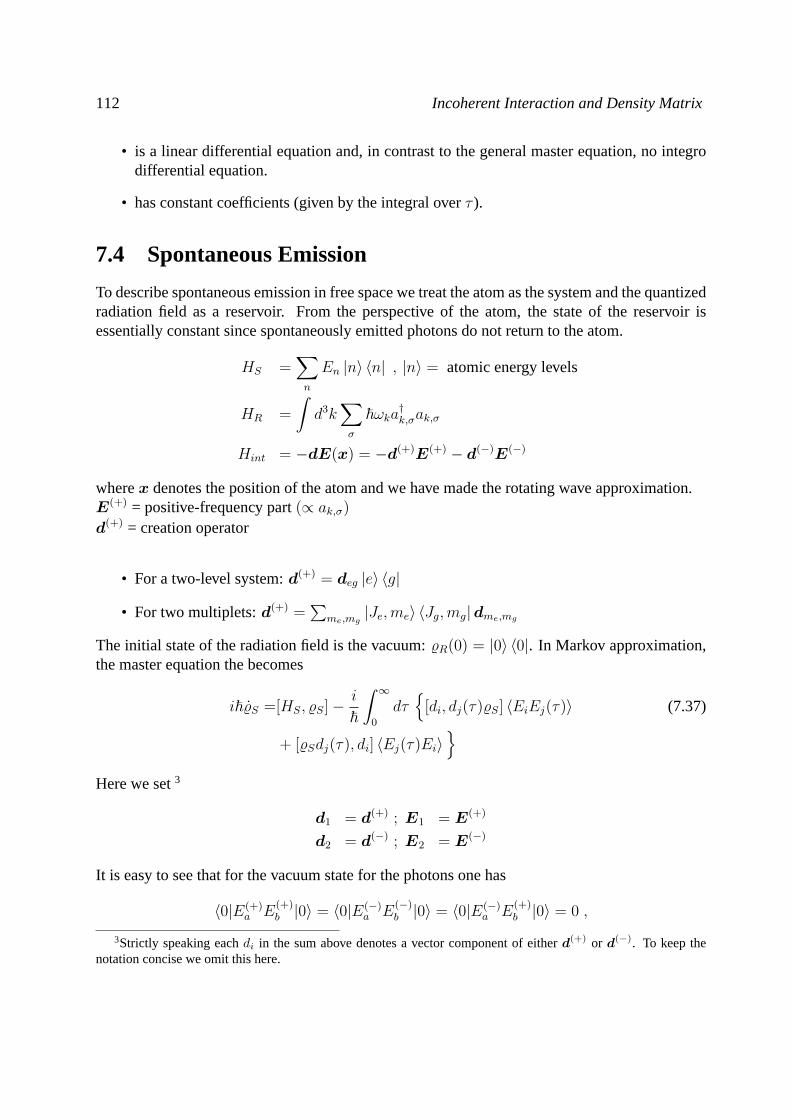
112 Incoherent Interaction and Density Matrix
• is a linear differential equation and, in contrast to the general master equation, no integrodifferential equation.
• has constant coefficients (given by the integral overτ ).
7.4 Spontaneous Emission
To describe spontaneous emission in free space we treat the atom as the system and the quantizedradiation field as a reservoir. From the perspective of the atom, the state of the reservoir isessentially constant since spontaneously emitted photons do not return to the atom.
HS =∑n
En |n〉 〈n| , |n〉 = atomic energy levels
HR =
∫d3k
∑σ
~ωka†k,σak,σ
Hint = −dE(x) = −d(+)E(+) − d(−)E(−)
wherex denotes the position of the atom and we have made the rotating wave approximation.E(+) = positive-frequency part(∝ ak,σ)
d(+) = creation operator
• For a two-level system:d(+) = deg |e〉 〈g|
• For two multiplets:d(+) =∑
me,mg|Je,me〉 〈Jg,mg|dme,mg
The initial state of the radiation field is the vacuum:%R(0) = |0〉 〈0|. In Markov approximation,the master equation the becomes
i~%S =[HS, %S]−i
~
∫ ∞0
dτ
[di, dj(τ)%S] 〈EiEj(τ)〉 (7.37)
+ [%Sdj(τ), di] 〈Ej(τ)Ei〉
Here we set3
d1 = d(+) ; E1 = E(+)
d2 = d(−) ; E2 = E(−)
It is easy to see that for the vacuum state for the photons one has
〈0|E(+)a E
(+)b |0〉 = 〈0|E(−)
a E(−)b |0〉 = 〈0|E(−)
a E(+)b |0〉 = 0 ,
3Strictly speaking eachdi in the sum above denotes a vector component of eitherd(+) or d(−). To keep thenotation concise we omit this here.
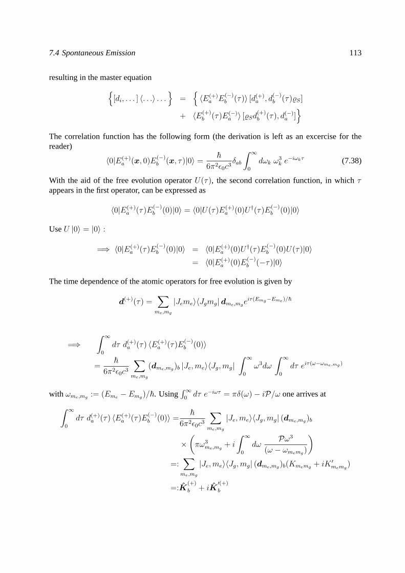
7.4 Spontaneous Emission 113
resulting in the master equation[di, . . . ] 〈. . .〉 . . .
=
〈E(+)
a E(−)b (τ)〉 [d(+)
a , d(−)b (τ)%S]
+ 〈E(+)b (τ)E(−)
a 〉 [%Sd(+)b (τ), d(−)
a ]
The correlation function has the following form (the derivation is left as an excercise for thereader)
〈0|E(+)a (x, 0)E
(−)b (x, τ)|0〉 =
~6π2ε0c3
δab
∫ ∞0
dωk ω3k e−iωkτ (7.38)
With the aid of the free evolution operatorU(τ), the second correlation function, in whichτappears in the first operator, can be expressed as
〈0|E(+)a (τ)E
(−)b (0)|0〉 = 〈0|U(τ)E(+)
a (0)U †(τ)E(−)b (0)|0〉
UseU |0〉 = |0〉 :
=⇒ 〈0|E(+)a (τ)E
(−)b (0)|0〉 = 〈0|E(+)
a (0)U †(τ)E(−)b (0)U(τ)|0〉
= 〈0|E(+)a (0)E
(−)b (−τ)|0〉
The time dependence of the atomic operators for free evolution is given by
d(+)(τ) =∑me,mg
|Jeme〉〈Jgmg|dme,mgeiτ(Emg−Eme )/~
=⇒∫ ∞
0
dτ d(+)a (τ) 〈E(+)
a (τ)E(−)b (0)〉
=~
6π2ε0c3
∑me,mg
(dme,mg)b |Je,me〉〈Jg,mg|∫ ∞
0
ω3dω
∫ ∞0
dτ eiτ(ω−ωme,mg )
with ωme,mg := (Eme − Emg)/~. Using∫∞
0dτ e−iωτ = πδ(ω)− iP/ω one arrives at∫ ∞
0
dτ d(+)a (τ) 〈E(+)
a (τ)E(−)b (0)〉 =
~6π2ε0c3
∑me,mg
|Je,me〉〈Jg,mg| (dme,mg)b
×(πω3
me,mg+ i
∫ ∞0
dωPω3
(ω − ωmemg)
)=:∑me,mg
|Je,me〉〈Jg,mg| (dme,mg)b(Kmemg + iK ′memg)
=:K(+)
b + iK′(+)
b
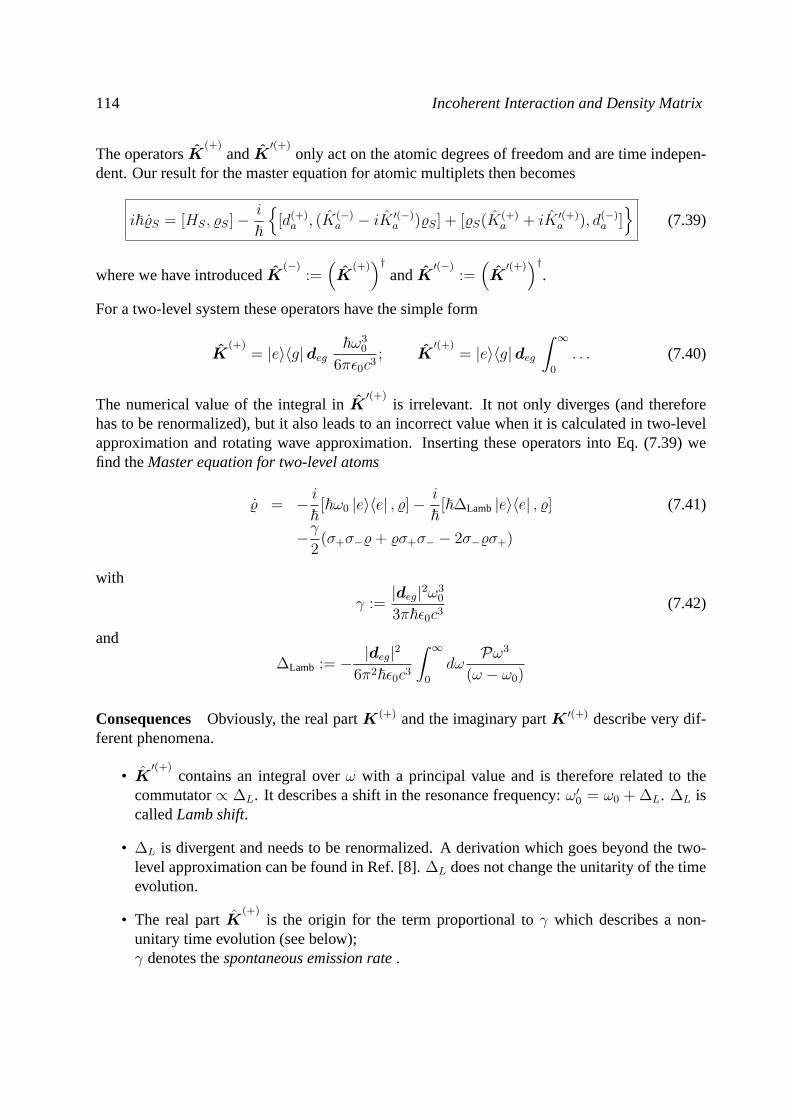
114 Incoherent Interaction and Density Matrix
The operatorsK(+)
andK′(+)
only act on the atomic degrees of freedom and are time indepen-dent. Our result for the master equation for atomic multiplets then becomes
i~%S = [HS, %S]−i
~
[d(+)a , (K(−)
a − iK ′(−)a )%S] + [%S(K
(+)a + iK ′(+)
a ), d(−)a ]
(7.39)
where we have introducedK(−)
:=(K
(+))†
andK′(−)
:=(K′(+))†
.
For a two-level system these operators have the simple form
K(+)
= |e〉〈g|deg~ω3
0
6πε0c3; K
′(+)= |e〉〈g|deg
∫ ∞0
. . . (7.40)
The numerical value of the integral inK′(+)
is irrelevant. It not only diverges (and thereforehas to be renormalized), but it also leads to an incorrect value when it is calculated in two-levelapproximation and rotating wave approximation. Inserting these operators into Eq. (7.39) wefind theMaster equation for two-level atoms
% = − i
~[~ω0 |e〉〈e| , %]−
i
~[~∆Lamb |e〉〈e| , %] (7.41)
−γ2(σ+σ−%+ %σ+σ− − 2σ−%σ+)
with
γ :=|deg|2ω3
0
3π~ε0c3(7.42)
and
∆Lamb := − |deg|2
6π2~ε0c3
∫ ∞0
dωPω3
(ω − ω0)
Consequences Obviously, the real partK(+) and the imaginary partK ′(+) describe very dif-ferent phenomena.
• K′(+)
contains an integral overω with a principal value and is therefore related to thecommutator∝ ∆L. It describes a shift in the resonance frequency:ω′0 = ω0 + ∆L. ∆L iscalledLamb shift.
• ∆L is divergent and needs to be renormalized. A derivation which goes beyond the two-level approximation can be found in Ref. [8].∆L does not change the unitarity of the timeevolution.
• The real partK(+)
is the origin for the term proportional toγ which describes a non-unitary time evolution (see below);γ denotes thespontaneous emission rate.
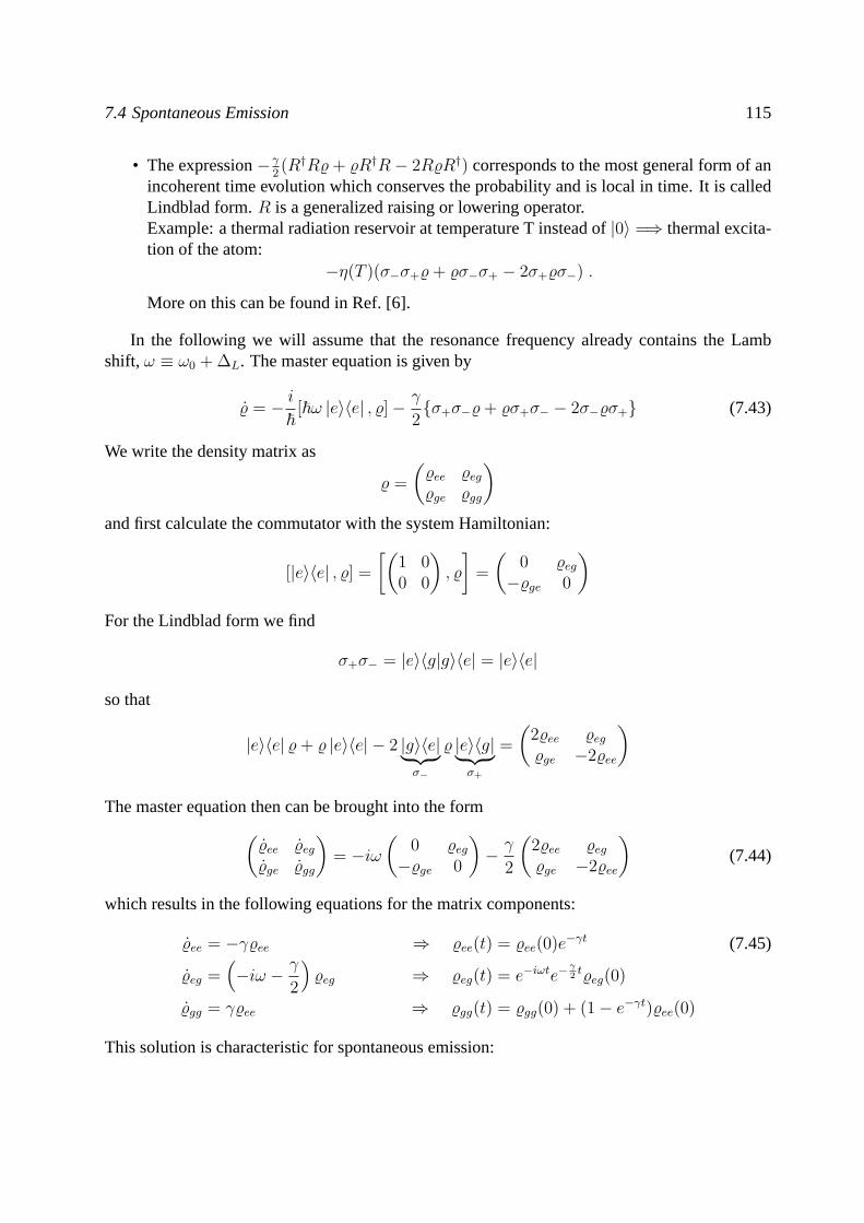
7.4 Spontaneous Emission 115
• The expression−γ2(R†R%+ %R†R− 2R%R†) corresponds to the most general form of an
incoherent time evolution which conserves the probability and is local in time. It is calledLindblad form.R is a generalized raising or lowering operator.Example: a thermal radiation reservoir at temperature T instead of|0〉 =⇒ thermal excita-tion of the atom:
−η(T )(σ−σ+%+ %σ−σ+ − 2σ+%σ−) .
More on this can be found in Ref. [6].
In the following we will assume that the resonance frequency already contains the Lambshift,ω ≡ ω0 + ∆L. The master equation is given by
% = − i
~[~ω |e〉〈e| , %]− γ
2σ+σ−%+ %σ+σ− − 2σ−%σ+ (7.43)
We write the density matrix as
% =
(%ee %eg%ge %gg
)and first calculate the commutator with the system Hamiltonian:
[|e〉〈e| , %] =
[(1 00 0
), %
]=
(0 %eg
−%ge 0
)For the Lindblad form we find
σ+σ− = |e〉〈g|g〉〈e| = |e〉〈e|
so that
|e〉〈e| %+ % |e〉〈e| − 2 |g〉〈e|︸ ︷︷ ︸σ−
% |e〉〈g|︸ ︷︷ ︸σ+
=
(2%ee %eg%ge −2%ee
)
The master equation then can be brought into the form(%ee %eg%ge %gg
)= −iω
(0 %eg
−%ge 0
)− γ
2
(2%ee %eg%ge −2%ee
)(7.44)
which results in the following equations for the matrix components:
%ee = −γ%ee ⇒ %ee(t) = %ee(0)e−γt (7.45)
%eg =(−iω − γ
2
)%eg ⇒ %eg(t) = e−iωte−
γ2t%eg(0)
%gg = γ%ee ⇒ %gg(t) = %gg(0) + (1− e−γt)%ee(0)
This solution is characteristic for spontaneous emission:
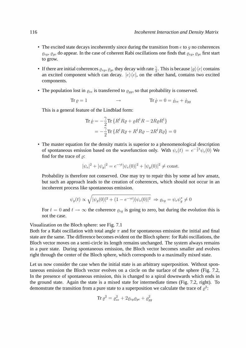
116 Incoherent Interaction and Density Matrix
• The excited state decays incoherently since during the transition frome to g no coherences%eg, %ge do appear. In the case of coherent Rabi oscillations one finds that%eg, %ge first startto grow.
• If there are initial coherences%eg, %ge they decay with rateγ2. This is because|g〉〈e| contains
an excited component which can decay.|e〉〈e|, on the other hand, contains two excitedcomponents.
• The population lost in%ee is transferred to%gg, so that probability is conserved.
Tr % = 1 → Tr % = 0 = %ee + %gg
This is a general feature of the Lindblad form:
Tr % = −γ2
Tr R†R%+ %R†R− 2R%R†
= −γ2
Tr R†R%+R†R%− 2R†R% = 0
• The master equation for the density matrix is superior to a phenomenological descriptionof spontaneous emission based on the wavefunction only. Withψe(t) = e−
γ2tψe(0) We
find for the trace of%:
|ψe|2 + |ψg|2 = e−γt|ψe(0)|2 + |ψg(0)|2 6= const.
Probability is therefore not conserved. One may try to repair this by some ad hov ansatz,but such an approach leads to the creation of coherences, which should not occur in anincoherent process like spontaneous emission.
ψg(t) ∝√|ψg(0)|2 + (1− e−γt)|ψe(0)|2 ⇒ %eg = ψeψ
∗g 6= 0
For t = 0 andt → ∞ the coherence%eg is going to zero, but during the evolution this isnot the case.
Visualization on the Bloch sphere: see Fig. 7.1Both for a Rabi oscillation with total angleπ and for spontaneous emission the initial and finalstate are the same. The difference becomes evident on the Bloch sphere: for Rabi oscillations, theBloch vector moves on a semi-circle its length remains unchanged. The system always remainsin a pure state. During spontaneous emission, the Bloch vector becomes smaller and evolvesright through the center of the Bloch sphere, which corresponds to a maximally mixed state.
Let us now consider the case when the initial state is an arbitrary superposition. Without spon-taneous emission the Bloch vector evolves on a circle on the surface of the sphere (Fig. 7.2,In the presence of spontaneous emission, this is changed to a spiral downwards which ends inthe ground state. Again the state is a mixed state for intermediate times (Fig. 7.2, right). Todemonstrate the transition from a pure state to a superposition we calculate the trace of%2:
Tr %2 = %2ee + 2%eg%ge + %2
gg
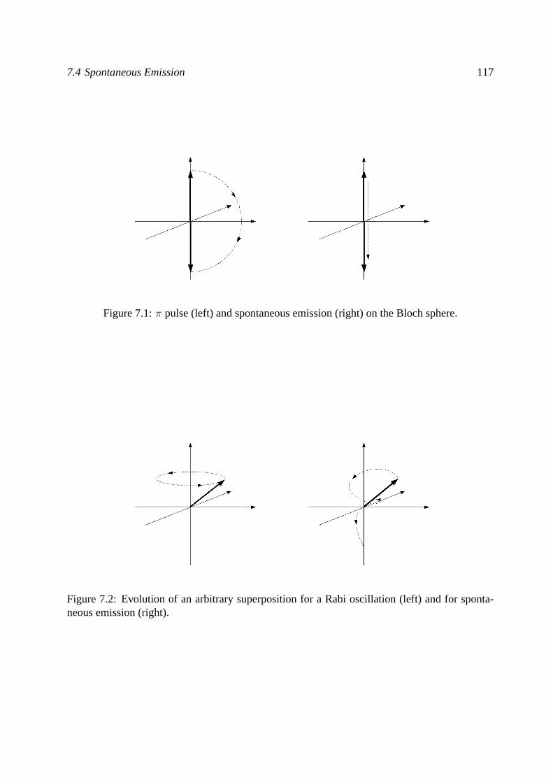
7.4 Spontaneous Emission 117
Figure 7.1:π pulse (left) and spontaneous emission (right) on the Bloch sphere.
Figure 7.2: Evolution of an arbitrary superposition for a Rabi oscillation (left) and for sponta-neous emission (right).
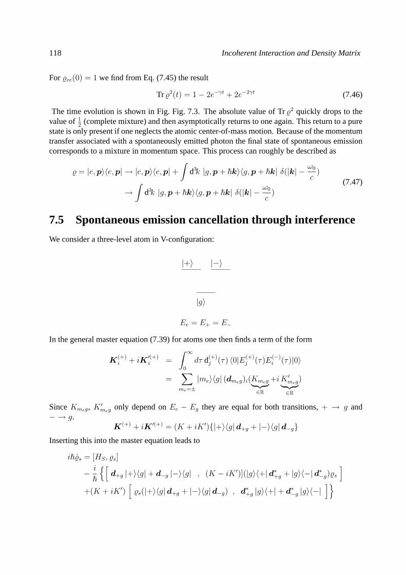
118 Incoherent Interaction and Density Matrix
For%ee(0) = 1 we find from Eq. (7.45) the result
Tr %2(t) = 1− 2e−γt + 2e−2γt (7.46)
The time evolution is shown in Fig. Fig. 7.3. The absolute value of Tr%2 quickly drops to thevalue of 1
2(complete mixture) and then asymptotically returns to one again. This return to a pure
state is only present if one neglects the atomic center-of-mass motion. Because of the momentumtransfer associated with a spontaneously emitted photon the final state of spontaneous emissioncorresponds to a mixture in momentum space. This process can roughly be described as
% = |e,p〉〈e,p| → |e,p〉〈e,p|+∫
d3k |g,p + ~k〉〈g,p + ~k| δ(|k| − ω0
c)
→∫
d3k |g,p + ~k〉〈g,p + ~k| δ(|k| − ω0
c)
(7.47)
7.5 Spontaneous emission cancellation through interference
We consider a three-level atom in V-configuration:
|g〉
|+〉 |−〉
Ee = E+ = E−
In the general master equation (7.39) for atoms one then finds a term of the form
K(+)i + iK
′(+)i =
∫ ∞0
dτ d(+)j (τ) 〈0|E(+)
j (τ)E(−)i (τ)|0〉
=∑me=±
|me〉〈g| (dmeg)i(Kmeg︸ ︷︷ ︸∈R
+iK ′meg︸ ︷︷ ︸∈R
)
SinceKmeg, K′meg only depend onEe − Eg they are equal for both transitions,+ → g and
− → g.K(+) + iK ′(+) = (K + iK ′)|+〉〈g|d+g + |−〉〈g|d−g
Inserting this into the master equation leads to
i~%s = [HS, %s]
− i
~
[d+g |+〉〈g|+ d−g |−〉〈g| , (K − iK ′)](|g〉〈+|d∗+g + |g〉〈−|d∗−g)%s
]+(K + iK ′)
[%s(|+〉〈g|d+g + |−〉〈g|d−g) , d∗+g |g〉〈+|+ d∗−g |g〉〈−|
]
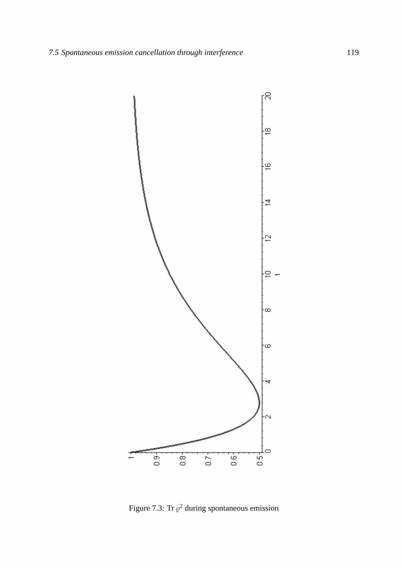
7.5 Spontaneous emission cancellation through interference 119
Figure 7.3: Tr%2 during spontaneous emission
120 Incoherent Interaction and Density Matrix
Under theassumptionthat4 d+ = d− = d this can be reduced to
i~%s = [HS, %s]−i
~|d|2
(K − iK ′)
[(|+〉+ |−〉) 〈g| , |g〉 (〈+|+ 〈−|) %s
]+(K + iK ′)
[%s (|+〉+ |−〉) 〈g| , |g〉 (〈+|+ 〈−|)
] (7.48)
If the atoms initially are in the special excited state|ψ〉 = 1√2(|+〉 − |−〉) we find
%s(0) = |ψ〉〈ψ| , HS |ψ〉 = Ee |ψ〉 → [HS, %s(0)] = 0
In addition we have(〈+|+ 〈−|) |ψ〉 = 0. Because of the term%s(|+〉+ |−〉) = 0 that appears inthe commutators in Eq. (7.48) one then finds
%s = 0
⇒ |ψ〉 can not decay into the ground state!
• Destructive interference between the decay amplitudes of|+〉 and|−〉 causes this super-position to be stable [14].
• This effect reminds us of the dark state in aΛ-system. The major difference is that|ψ〉 isan excited state and represents a dark state for all resonant photons.
• The observation of this effect is difficult since the assumptiond+ = eiαd− cannot befullfilled for atoms. This is because atomic energy eigenstates are eigenstates ofJz
Example: three-level system inV configuration:
Jg = 0 Je = 1
3
QQQk
One then has
d+ = D(ex − iey)/√
2 couples toσ+ light
d− = D(ex + iey)/√
2 couples toσ− light
Thus,d+ ·d∗− = 0 and the interference terms in the master equation are zero. For instance,we have
(|+〉d+ + |−〉d−) 〈g| · |g〉 (〈+|d∗+ + 〈−|d∗−) = D2(|+〉〈+|+ |−〉〈−|) .
By contrast, under the assumptiond+ = d− used above one finds
D2(|+〉 + |−〉)(〈+| + 〈−| .
• For molecules destructive interference is possible in principle. Experimental observationof spontaneous emission cancellation was reported in Ref. [15], but the result was laterquestioned [16].
4The choiced+ = eiαd− is also possible.
Chapter 8
Laser”=K uhlen von Atomen
8.1 Allgemeines zur Kuhlung von Atomen
Nach dem Satz von Liouville kann man die Entropie eines abgeschlossenen (Quanten)”=Systemsnicht andern, da es sich unitar entwickelt. Adiabatisches Kuhlen zur Verringerung der Temper-atur ist zwar moglich (sieheUbungen), die Entropie (
”Unordnung “) bleibt dabei aber erhalten.
Um die Unordnung zu verringern bzw. das von den Atomen besetzte Phasenraumvolumenzu verkleinern muss das System offen sein. Die Beschreibung des Systems kann dann durch eineMaster”=Gleichung erfolgen.
Verschiedene Konzepte der Kuhlung
• Austausch von Atomen mit der Umgebung. z.B. Verdampfungskuhlen wie bei der Kaffee-tasse (bzw. bei Corinnas Teetasse). Hierbei befinden sich die Atome in einem Potentialtopfendlicher Tiefe. Nur die heißesten Atome haben genug Energie, um den Topf zu verlassen.Die verbliebenen Atome sind dann im Mittel kalter. Durch Stoße zwischen den Atomenwerden die Atome rethermalisiert, so dass die Energieverteilung wieder thermisch wird.
• Spontan emittierte Photonen dissipieren Energie und Impuls. (Induzierte Emission tut diesnicht, da dies ein unitarer Prozess ist).⇐⇒ Laser-Kuhlen. Nobelpreis 1997 an ClaudeCohen-Tannoudji, Steve Chu und Bill Phillips
Eine ausgezeichnete Einfuhrung in die Konzepte der Laserkuhlung kann man in Ref. [12]finden.
8.2 Doppler”=Kuhlung
Die Doppler-Kuhlung ist die grundlegendste Form der Laser”=Kuhlung (Lethokov, Hansch undSchawlow 1975).
122 Laser”=Kuhlen von Atomen
8.2.1 Das Prinzip
Die Anregungswahrscheinlichkeit der Atome hangt von der Laser”=Frequenz ab (sieheUbun-gen).
%ee =|Ω|2
∆2 + γ2
4+ 2|Ω|2
(8.1)
wobei∆ = ωL−ω0 undΩ die Rabi-Frequenz ist. Der mittlere absorbierte Impuls ist~kL%ee(ωL).Bewegt sich das Atom mit der Geschwindigkeitv, so nimmt es eine durch den Doppler-
Effekt verschobene Laser”=Frequenzω′L = ωL − kL · v wahr:
• fur v parallel zukL ist ω′L rotverschoben (ω′L < ωL)
• fur v antiparallel zukL ist ω′L blauverschoben (ω′L > ωL)
Nun wahlt man∆L = ωL − ω0 < 0, also einen rotverstimmten Laser. Fur Atome, die aufden Laser zufliegen, ist die Verstimmung gegeben durch
∆′ = ω′L − ω0 = ωL − kL · v − ω0 = ∆L − kL · v (8.2)
so dass|∆′| < |∆L| (solangev nicht zu groß ist). Ein rotverstimmter Laser regt deshalb vornehm-lich Atome an, die auf ihn zufliegen.
Bei zwei gegenlaufigen rotverstimmten Laserstrahlen werden die Atome vornehmlich Photo-nen von dem Laserstrahl absorbieren, auf den sie zufliegen. Dadurch werden die Atome gekuhlt.
8.2.2 Theoretische Beschreibung
Man beschreibt das Problem durch:
H =p2
2M− ~∆ |e〉〈e| − ~Ω(x) |e〉〈g| − ~Ω∗(x) |g〉〈e| (8.3)
(Zwei-Niveau-Atom mit Schwerpunktbewegung im Laserfeld). Zu losen ist die DGL:
% = − i
~[H, %]− γ
2σ+σ−%+ %σ+σ− − 2σ−%σ+ (8.4)
Der letzte Termσ−%σ+ ist dabei anders als im vorigen Kapitel, da der Impulsubertrag derspontan emittierten Photonen berucksichtigt werden muss:
σ−%σ+ = |g〉〈g| %ee (8.5)
σ−%σ+ =
∫d2Ω
8π/3
(1− |deg · k|2
)eikx%eee
−ikx |g〉〈g| (8.6)
Wobei(1− |deg · k|2
)die Dipol-Charakteristik beschreibt,eikx den Impulsubertrag von~k,
%ee ist 〈e|%|e〉. Herleitung: Siehe Ref. [13]. Dieser Term”heizt “ die Atome, da er∆p um etwa
8.2 Doppler”=Kuhlung 123
~k vergroßert.
Losungsidee fur die MastergleichungVerwende die Born-Oppenheimer Naherung (oder adiabatische Naherung): Die Schwerpunktbe-wegung ist viel langsamer als die elektronische Relativbewegung, daher lost man das elektronis-che Problem fur fixiertesx und setzt dies in die Schwerpunkt-DGL ein.
Die interne Zeitentwicklung ist sogar so schnell, dass man einfach die stationare elektromag-netische Losung nehmen kann.
%!= 0 = − i
~[H, %]− γ
2σ+σ−%+ %σ+σ− − 2σ−%σ+ (8.7)
mit
H = ~(
−∆ −Ω(x)−Ω∗(x) 0
)(8.8)
Die Losung dieses Problems ist:
%ee =|Ω|2
L%eg = −
Ω(∆− iγ
2
)L
= %∗ge (8.9)
wobei L := ∆2L + γ2
4+ 2|Ω|2. Dies setzt man in die Schwerpunktbewegung ein und lasst
hier der Einfachheit halber den dissipativen Term∫
d2Ω8π/3
. . . weg (weiter unten werden wir ihnphanomenologisch wieder einfuhren). So ergibt sich:
H =p2
2M− d ·E(x) + innere Zustande (8.10)
Daraus folgen:
x =p
M(8.11)
p = ∇(d ·E(x)) (8.12)
Dies sind die Heisenberg-Bewegungsgleichungen fur x undp.Wir benutzen wieder die RWA:
d ·E(x)RWA= deg ·E(+)(x) |e〉〈g|+ d∗eg ·E(−)(x) |g〉〈e|
= ~Ω(x) |e〉〈g|+ ~Ω∗(x) |g〉〈e| (8.13)
Der Mittelwertuber die inneren Freiheitsgrade ergibt
˙p = Tr 2×2(%p)
= ~ Tr 2×2(%|e〉〈g|∇Ω(x) + |g〉〈e|∇Ω∗(x))= ~(∇Ω(x))%ge + ~(∇Ω∗(x))%eg (8.14)
124 Laser”=Kuhlen von Atomen
Einsetzen von%eg und%ge = %∗eg = −Ω∗(∆+i γ2)
L.
˙p = F = −~∆L∇(|Ω|2)
L− i~
γ
2
Ω∗(∇Ω)− Ω(∇Ω∗)
L
= −~∆L
2∇ ln
(∆2L +
γ2
4+ 2|Ω|2
)− i
~γ2
Ω∗(∇Ω)− Ω(∇Ω∗)
∆2L + γ2
4+ 2|Ω|2
(8.15)
Der erste Term ist eine konservative Kraft (da= ∇...), der zweite Term stellt eine dissipativeKraft dar.
F = −~∆L1
2∇ ln
(∆2L +
γ2
4+ 2|Ω|2
)− i~
γ
2
Ω∗∇Ω− Ω∇Ω∗
∆2L + γ2
4+ 2|Ω|2
(8.16)
Beispiel 1: laufende Laserwelle:Ω = Ω0 · eikx, |Ω|2 = Ω20 ∈ R
=⇒ F = ~kγΩ2
0
∆2L + γ2
4+ 2Ω2
0
= ~kγ%ee (8.17)
Doppler-Effekt:
∆L −→ ∆L − kv = ∆L −pk
M
=⇒ F = ~kγΩ2
0(∆L − kp
M
)2+ γ2
4+ 2Ω2
0
(8.18)
Beispiel 2: Zwei gegenlaufige Laser. Wir behandeln das Problem vereinfacht, indem wir dieKrafte vonΩ1 = Ω0e
ikx undΩ2 = Ω0e−ikx addieren1.
F = F→ + F←
= ~ k γ Ω20
4∆L · kpM
[(∆L − kpM
)2 + γ2
4][(∆L + kp
M)2 + γ2
4]
(8.19)
(fur Ω0 γ). Dabei istF← = F→(−k). Fur kleines p gilt
F ≈ 4 ~ k
Mγ Ω2
0 k p∆L(
∆2L + γ2
4
)2 ∼ p
In Richtung vonk haben wirFp < 0 fur ∆L < 0, so dass aus der Bewegungsgleichungp =F die Zeitentwicklungp(t) ∼ e−αt abgeleitet werden kann. Der mittlere Impuls wird somitabgebremst. WegenF ∼ γ ist dafur die spontane Emission notwendig. Die maximale KraftF
wird erreicht fur ∆L = −γ2
und ist gegeben durchF = −8 ~ k2
M
Ω20
γ2 p.
1Eigentlich muss manΩ = Ω0 cos(kx) setzen und vollig anders weiterrechnen. Dies fuhrt zu kompliziertenBerechnungen. Qualitativ richtig und viel einfacher ist der Zugang, den wir hier verwenden.
8.3 VSCPT 125
Diese Kraft muss verglichen werden mit der (noch nicht berucksichtigten) Heizrate, die sichdurch den Impulsubertrag der spontan emittierten Photonen ergibt. (=⇒ Impulsverteilung wirdverbreitert).
Heizrate intuitiv: die Breite der Impulsverteilung ist definiert alsσ2 = 〈p2〉−〈p〉2. Ihre durchdas Heizen verursachte zeitlicheAnderung genugt
d
dtσ2
∣∣∣∣Heiz
= Anregungswahrscheinlichkeit· Emissionsrate· Impulsubertrag2
= %ee · γ · ~2k2
Somit erhalten wir fur die gesamte (Kuhlen und Heizen)Anderung den Ausdruck
d
dtσ2 =
d
dtp2︸︷︷︸
2pp
+d
dtσ2︸︷︷︸
γ%ee~2k2
∣∣∣∣∣∣∣∣Heiz
Betrachten wir die Situation fur die maximale Kuhlungskraft, also∆L = −γ/2, so ist die An-regungswahrscheinlichkeit durch%ee = 2Ω2
0/γ2 gegeben. Im Gleichgewicht muß−2pF =
γ~2k2 · 2Ω20/γ
2 gelten, so dass man auf
p2
2M=
~γ16
=1
2kBT
schließen kann. Das stimmt bis auf einen numerischen Faktor. Das richtige Ergebnis ist das sog.Doppler-Limit:
kBT = ~γ γ ≈ 107 s−1 =⇒ T ≈ 10−4 K (8.20)
8.3 VSCPT
Velocity-selective coherent population trapping [20] verwendet Dunkelzustande zum Kuhlen undkann erst bei tiefen Temperaturen eingesetzt werden (< 10µK). Die Methode liefert dafur sehrtiefe Endtemperaturen (3 nK). Betrachte einΛ-System mit Schwerpunktbewegung:
|e,p〉
k−, ωL,Ω− Ω+, ωL,k+
Ee
Eg|−,p− ~k−〉 |+,p− ~k+〉
Dabei gilt:E+ = E− = Eg, ∆ = ωL − (Ee − Eg)/~, |k+| = |k−| = k
H =p2
2M1− ~∆ |e〉 〈e|
+ ~Ω−[eik−x |e〉 〈−|+ e−ik−x |−〉 〈e|
]+ ~Ω+
[eik+x |e〉 〈+|+ e−ik+x |+〉 〈e|
]= H0 +Hint
(8.21)
126 Laser”=Kuhlen von Atomen
i~ |ψ〉 = H |ψ〉 , entwickle|ψ〉 gemaß
|ψ〉 =
∫d3p ψe(p) |e,p〉
+ ψ+(p− ~k+) |+,p− ~k+〉+ ψ−(p− ~k−) |−,p− ~k−〉
Einsetzen=⇒
i~∂t
ψe(p)ψ+(p− ~k+)ψ−(p− ~k−)
=
−~∆ + p2
2M~Ω+ ~Ω−
~Ω+(p−~k+)2
2M0
~Ω− 0 (p−~k−)2
2M
ψe(p)ψ+(p− ~k+)ψ−(p− ~k−)
(8.22)
=⇒ Im allgemeinen ist die Entartung von|+〉, |−〉 durch die Schwerpunktbewegung aufgehoben.SetzeΩ+ = Ω− = Ω =⇒
|ψD(p)〉 =1√2|−,p− ~k−〉 − |+,p− ~k+〉 (8.23)
ist ein Dunkelzustand im Sinne vonHint |ψD(p)〉 = 0. Aber:
H0 |ψD(p)〉 =
(p2
2M+
~2k2
2M
)|ψD(p)〉
+1√2
−~k−p
M|−,p− ~k−〉+
~k+p
M|+,p− ~k+〉
k := k+ = k− =⇒ H0 |ψD(p)〉 =(p− ~k)2
2M|ψD(p)〉 : Eigenzustand
k := k+ = −k− =⇒ H0 |ψD(p)〉 =(p2 + ~2k2)
2M|ψD(p)〉 − ~kp
M|ψB(p)〉
=⇒ Bei gegenlaufigen Lasern (k+ = −k−) ist nur |ψD(0)〉 ein Eigenzustand vonH0 + Hint.Dies fuhrt uns zur Idee von VSCPT:
• Atome werden von den Lasern nach|e〉 angeregt und fallen via spontaner Emission zuruck.
• Atome, die nach|ψB(p)〉 fallen, werden wieder hochgepumpt
• Atome, die nach|ψD(p 6= 0)〉 fallen, entwickeln sich erst zu|ψB(p)〉 und werden danngepumpt
• Atome in|ψD(p = 0)〉 bleiben dort: Kuhlung.
Chapter 9
Electromagnetically induced transparency
EIT is one of many effects in quantum optics where light changes the state of the atoms, whichin turn leads to a change of the index of refraction. The description of such effects is based on
9.1 The Maxwell-Bloch equations
Equation for atoms:% = L% as in Chapter 7, with the interaction between light and atoms givenby
H = HA +HRad−1
ε0
∫P (x) ·D(x)d3x
P (x) = Polarization; e.g. for a single atom at positionx0 :
P (x) = dδ(x− x0)
(9.1)
Heisenberg’s equation of motion: (as in Chapter 2):
i~D(x) = [D(x), H] with
[Di(x), Bj(x′)] = −i~εijk∂kδ(x− x′)
(9.2)
from which follows
D =1
µ0
rotB (9.3)
B = − 1
ε0
rot (D − P ) (9.4)
These are Maxwell’s equations1 in a dielectric with polarizationP . As we have learned in thefirst chapters, one can deduce wave equations from these relations:(
1
c2∂2t + rot rot
)D = rot rotP , (9.5)
1We assume that the macroscopic free charge density vanishes, so that divD = 0. It is then not necessary todistinguish between the transverse part of the dielectric displacement field and the field itself.
128 Electromagnetically induced transparency
or, usingD = ε0E + P , (1
c2∂2t + rot rot
)E = −µ0P (9.6)
Together with% = L% this equation represents theMaxwell-Bloch equations. These equationsare generally hard to solve and one has to make approximations. Frequently used assumptionsare the following.
• Homogeneously distributed atoms
⇒ P (x, t) = P (t) (9.7)
• The atomic density is very low so that the atoms do not interact directly with each other(collisions) and do only interact with the light.
⇒ P (t) = %d (9.8)
here% denotes the atomic density andd the dipole moment operator for a single atom.
Averaging over the atomic degrees-of-freedom results in(1
c2∂2t + rot rot
)E = −µ0% 〈d〉 (9.9)
= − 1
c2ε0%Tr (%d) (9.10)
The Maxwell-Bloch equation allow to calculate the optical properties of an atomic medium.In a gas one can neglect interatomic collisions to a certain degree.
9.2 Index of refraction for a two-level atom
As in Chapter 8 we consider a two-level atom in a running laser beam,
E = E0eikxe−iωLt + c.c. . (9.11)
The laser beam is continuously switched on (“cw”) so that, after a short time, the atoms are welldescribed by their stationary state ,
%stee =|Ω|2
∆2 + γ2
4+ 2|Ω|2
%stgg = 1− %stee
%steg =−Ω(∆− iγ
2)
∆2 + γ2
4+ 2|Ω|2
(9.12)
∆ = ωL − ω0
9.2 Index of refraction for a two-level atom 129
This is the solution in the “co-rotating frame”, whereHA = ~∆ |e〉 〈e|. To get the solution in the“laboratory frame”, we need to perform the unitary transformationU = exp (−iωLt |e〉 〈e|). Itfollows that
%(t) = U(t)%stU+(t)
=∑i,j
%stijU |i〉 〈j|U+
= %stee |e〉 〈e|+ %stgg |g〉 〈g|+ %stege−iωLt |e〉 〈g|+ %stgee
iωLt |g〉 〈e| (9.13)
⇒ Tr (%(t)d) = deg%ge(t) + d∗eg%eg(t) (9.14)
The connection between the amplitude of the electric field and the Rabi frequency that ap-pears in the stationary density matrix (9.12) is given by
Ω(x, t) =1
~deg ·E(+)(t)
=1
~deg ·E0e
ikxe−iωLt (9.15)
Inserting this into Maxwell’s equation results in(1
c2∂2t + rot rot
)(E0e
ikxe−iωLt + E∗0e−ikxeiωLt
)=
ω2L%
c2ε0
(deg(−1)
∆ + iγ2
∆2 + γ2
4+ 2|Ω0|2
eiωLte−ikx 1
~d∗egE
∗0
+d∗eg(−1)∆− iγ
2
∆2 + γ2
4+ 2|Ω0|2
e−iωLteikx 1
~degE0
)(9.16)
with Ω0 = deg ·E0/~. Assuming thatE0 = const. we can compare the coefficients ofe±iωLt onboth sides of the equation, which results in
−ω2L
c2E0 − k × (k ×E0) =
−%ω2L
~ε0c2d∗eg(degE0)
∆− iγ2
∆2 + γ2
4+ 2|Ω0|2
(9.17)
Definedeg = Dε∗, E0 = E0ε with ε ⊥ k:
⇒ −ω2L
c2E0ε + k2εE0 = − %ω2
L
~ε0c2D2εE0
∆− iγ2
∆2 + γ2
4+ 2|Ω0|2
(9.18)
⇒ −ω2L
c2+ k2 =
−%ω2L
~ε0c2D2 ∆− iγ
2
∆2 + γ2
4+ 2|Ω0|2
(9.19)
This is an equation which connectsk with ωL. The frequencyωL is determined by the laser andis not changed inside the medium, since otherwise the boundary conditions between the medium
130 Electromagnetically induced transparency
and free space could not be fulfilled.k, on the other hand, can have a different value inside themedium thanωL
c. Solution:
k(ωL) =
√ω2L
c2− ω2
L
c2%D2
~ε0∆− iγ
2
∆2 + γ2
4+ 2|Ω0|2
(9.20)
where∆ = ωL − ω0
We can compare this with the definition of the index of refraction :
k(ωL) =ωLcn(ωL) (9.21)
⇒ n(ωL) =
√1− %D2
~ε0∆− iγ
2
∆2 + γ2
4+ 2|Ω0|2
(9.22)
Approximation for small densities:√
1− x = 1− 12x⇒
n(ωL) = 1− 1
2
%D2
~ε0∆− iγ
2
∆2 + γ2
4+ 2|Ω0|2
(9.23)
The index of refraction is generally complex,n = n′+ in
′′
⇒ E(+) = E0e−iωLteikx
ωLc
(n′+in
′′)
= E0e−iωLteik
′xe−k
′′x (9.24)
• The real partn′
determines the phase velocityvph = ωRek of the light. For vanishing
detuning the phase velocity becomesv(∆ = 0) = c.
• Group velocity: Consider a wavepacket
E(x, t) =
∫dωeik(ω)xe−iωtE(ω) (9.25)
For a narrow frequency widthω ≈ ω0, we can make the expansion
k(ω) ≈ k(ω0) +∂k
∂ω
∣∣∣∣ω0
(ω − ω0) + . . . (9.26)
⇒ E(x, t) =
∫dωE(ω)e−iωteik(ω0)xe
i ∂k∂ω |ω0
(ω−ω0)x
= eik(ω0)xe−i ∂k
∂ω |ω0ω0x∫
dωE(ω)e−iω(t− ∂k
∂ω |ω0x)
(9.27)
9.3 Electromagnetically induced transparency and dark states 131
We can infer that the wavepacket travels with a velocity determined by
x
t= const.=
(∂k
∂ω
)−1∣∣∣∣∣ω0
=∂ω
∂k
∣∣∣∣ω0
(9.28)
This corresponds to the group velocityvgr = ( ∂k∂ω
)−1. It varies particularly strong aroundthe resonance∆ = 0. However, at the same timen′′, which describes the absorption, ismaximal for∆ = 0. One therefore cannot consider this situation as a real propagation oflight since most of it is absorbed. The notion of a group velocity is then not very useful.
• “Spectral hole burning”:|Ω0|2 is proportional to the light intensity. Hence, for high inten-sities absorption (and all other effects) is strongly suppressed even if∆ = 0. The reasonis simply that a high intensity corresponds to many photons inside the medium. If allatoms have already been excited by a photon, the remaining photons cannot be absorbedanymore.
9.3 Electromagnetically induced transparency and dark states
The refraction index for atoms with more than two levels can be very different from the two-level result. One example is the phenomenon of electromagnetically induced transparency for athree-level atom inΛ configuration. To derive theindex of refraction we again have to solve theMaxwell-Bloch equations with
H = ~
0 −Ω− −Ω+
−Ω∗− ∆− 0−Ω∗+ 0 ∆+
Lsp. Em.% =
−γ%ee −γ2%e− −γ
2%e+
−γ2%−e
γ2%ee 0
−γ2%+e 0 γ
2%ee
(9.29)
Master equation:
% = − i
~[H, %] + Lsp. Em.%
!= 0 stationary solution (9.30)
To find the solution of this system of linear equations is simple in principle, but to reduce the sizeof the result we consider the case thatΩ+ is small and expand the solution aroundΩ+ = 0.ForΩ+ = 0, the soltution is simply the dark state , i.e.,
%0 = |+〉〈+| (9.31)
Since|+〉 is the dark state for the situationΩ+ = 0 andΩ− 6= 0, the entire population is pumpedinto the state|+〉.
If we switch on a weak second laser beam (Ω+ 6= 0) we can calculate its effect using pertur-bation theory:H = H0 + H1 with
H0 = ~
0 −Ω− 0−Ω∗− ∆− 0
0 0 ∆+
H1 = ~
0 0 −Ω+
0 0 0−Ω∗+ 0 0
(9.32)
132 Electromagnetically induced transparency
Inserting the ansatz% = %0 + %1 +O(Ω2+) into (9.30) we find
0 = − i
~[H0 +H1, %0 + %1] + Lsp.Em.%0 + Lsp.Em.%1 (9.33)
Since%0 is the solution of the unperturbed equation, we find for the equation to first order inH1
− i
~[H0, %1] + Lsp.Em.%1 =
i
~[H1, %0] (9.34)
This is an inhomogeneous linear system of equations for%1. The solution is given by
% = |+〉〈+|︸ ︷︷ ︸%0
+ %e+ |e〉〈+|+ %−+ |−〉〈+|+ H.c. (9.35)
with
%e+ = − (∆− −∆+)Ω+
(∆− −∆+)(∆+ + iγ2) + |Ω−|2
%−+ =−Ω+Ω∗−
(∆− −∆+)(∆+ + iγ2) + |Ω−|2
We now calculate the index of refraction for theΩ+ beam with the aid of Eq. (9.9). We knowfrom the derivation of the two-level refraction index in Sec. 9.2 that2
n+ ≈ 1 +%D2~ε0
Tr (d(−)· ε∗Ω+
%)1
Ω+(9.36)
For theΩ+ beam we haved(−)· ε∗Ω+
∝ |+〉〈e|, so that
n+ ≈ 1− %D2
2~ε0
∆− −∆+
(∆− −∆+)(∆+ + iγ2) + |Ω−|2
(9.37)
The prefactor%D2/(2~ε0) is typical for optically thin gases and also appears in the two-levelresult. The term after the prefactor is responsible for EIT.
For ∆− = ∆+ we haven = 1, i.e., the same refraction index as in free space; in particular,there is no absorption and the phase velocity isc. However, the system does not completelybeahve as a vacuum since the right-hand side is trivial only exactly at resonance. The groupvelocity ∂ω
∂kis different from its vacuum value.
Let us consider the case∆− = 0 (pump laser in resonance):
n+ = 1− %D2
2~ε0
(ω0 − ω+)
(ω0 − ω+)(ω+ − ω0 + iγ2) + |Ω−|2
(9.38)
2The derivation of this equation is completely analogous to that of Eq. (9.23).
9.3 Electromagnetically induced transparency and dark states 133
We have for the wave vector
k+(ω+) =ω+
cn+(ω+) (9.39)
It is then easy to calculate the group velocity,
∂k+
∂ω+
∣∣∣∣ω+=ω0
=n+
c− ω+
c
∂n+
∂ω+
= . . . =1
c+ω0
c
%D2
2~ε0
1
|Ω−|2(9.40)
⇒ vgr =c
1 + %D2
2~ε0ω0
|Ω−|2(9.41)
In principle this would allow us to achievevgr = 0 (for Ω− → 0). However, in this limit theexpansion (Ω+ Ω−) we have made is not valid anymore. Nevertheless, this limit has beenachieved experimentally.
Example ω0 = 1015 s−1, D = ea0, % ≈ 1021 m−3, Ω− ≈ 108 s−1. This results in a groupvelocity of
vgr =1
310−6c ≈ 100
m
s(9.42)
The first experiment by the group of Lene Hau [21] achievedvgr = 17 m/s in 1999. A yearlater the group of Philipps sogar was able to stop light completely [34]. Stopping of light can beunderstood as a transfer of atoms from|+〉 to |−〉 followed by switching off the pump laser. Theinformation about the probe pulse is then coherently and reversibly stored in the medium. TheΩ+ pulse can be restored after up to a millisecond [35].

134 Electromagnetically induced transparency
Chapter 10
Photonic band gaps
Photonic band gaps (PBG) are completely analogous to the energy bands of electrons in a pe-riodic potential which are well-known in solid state physics. Their physical meaning is that ina periodic dielectric photons cannot propagate at certain frequencies (inside a band gap). Onecan create such band gaps by a periodic modulation of the index of refraction. To simplify thenotation we introduce the relative dielectric constantεr,
εr(x) =ε(x)
ε0
= n2(x) n: index of refraction (10.1)
which we assume to be time-independent (εr ∝ ε(x) = 0). We then have
D = ε0E + P = ε(x)E = ε0εr(x)E(x) (10.2)
and Maxwell’s equations become
B = −rotE D = ε0c2rotB (10.3)
which leads to a “symmetric” wave equation forB:(∂2t + c2rot
1
εr(x)rot
)B(x, t) = 0 (10.4)
Consider now a periodic index of refraction (or dielectric factor)εr(x) = εr(x + L), which forsimplicity only depends onx 1. To emphasize the analogy between photonic and elektronic bandgaps we will treat the wave equation with concepts borrowed from quantum mechanics.
• We first define a conserved scalar product (see also Sec. 2.1.6), which will allow us tointroduce Hermitean operators:
〈B|B′〉 := −iε0
~
∫d3x (B
∗B′ −B∗B
′) (10.5)
⇒ ∂t 〈B|B′〉 ∝∫d3x (B
∗B′ −B∗B
′) (10.6)
1In the following we will nevertheless use the notationεr(x) for a dependence on all components if the equationis generally valid.
136 Photonic band gaps
inserting this into the wave equation (10.4)
=
∫d3x
[(−c2rot
1
εr(x)rotB∗)B′ −B∗(−c2rot
1
εr(x)rotB′)
](10.7)
=
∫d3x
[B∗(−c2rot
1
εr(x)rotB′)−B∗(−c2rot
1
εr(x)rotB′)
]= 0
(10.8)
In the last step we have performed two partial integrations to move the curl operator to theprimed part. We also used thatεr(x) does not depend on time and appears between thetwo curl operators.
• The “Hamiltonian” operatorH := −c2rot εr(x)−1rot is Hermitean, i.e.,〈B′|HB〉 =〈HB′|B〉. In addition,H is periodic,H(x+ L) = H(x).
To derive the eigenmodes of the wave equation (10.4) we prooced analogously to solid statetheory and first consider the Translation operator translation operator
Tx0 = eibp·x0/~ = ex0·∇x (10.9)
Effect of operator: (Tx0f)(x) = f(x + x0) (10.10)
Proof: Tx0f(x) = ex0·∇xf(x)
=∞∑n=0
(x0 ·∇x)n
n!f(x) ≡ Taylor-Reihe umx
= f(x + x0) (10.11)
H commutes withTL,
(HTL − TLH)f(x) = Hf(x+ L)−H(x+ L)f(x+ L) = 0 ,
becauseH is periodic. Hence,H andTL share a common system of eigenstates.The eigenstates ofTL are the momentum stateseikx with eigenvaluesTLeikx = eik(x+L) =
eikLeikx. This means the eigenvalues are degenerate for all momenta of the formk = q+ 2nπL, n ∈
Z with eigenvalueexp(iqL).The eigenstates ofH can be written as a superposition of degenerate eigenstates ofTL,
ψq(x) = eiqx∞∑
n=−∞
ψq,nei 2nπ
Lx (10.12)
The quantum numberq can be chosen to be in the interval[−π2, π
2] 2. q is calledquasi momentum
(= momentum modulo2π/L).
2Another choice can be made by changing the sumation index. For instance, forq′ = q+ 2π/L we get the sameexpansion as above ifψq,n is replaced byψq′,n−1.
137
Eigenvalue problem:(∂2
∂t2−H
)ψ = 0, Ansatzψ(x, t) = e±iωtψ(x) ⇒ −ω2ψ(x) =
Hψ(x)Here we consider the most simple case:
εr = 1 + δε cos
(2π
Lx
)with δε 1 ⇒
H = −c2rot1
1 + δε cos(
2πLx) rot
≈ −c2rot
(1− δε cos
(2π
Lx
))rot
= H0 + δεH1
with
H0 = −c2rot rot
H1 = c2rot cos
(2π
Lx
)rot
Consider a light wave along thex axis,
B(x) = B(x)ey
This ansatz fulfills the Maxwell equation divB = 0. The action of the Hamiltonian becomes(−rot
1
εr(x)rotB
)=
(∂
∂x
1
εr(x)
∂
∂xB
)ey
We now employ perturbation theory,B(x) = 〈x|B〉, |B〉 = |B0〉 + δε |B1〉, where|B0〉 is amomentum eigenstatep0.
(H0 + δεH1) (|B0〉+ δε |B1〉) = −ω2 (|B0〉+ δε |B1〉) with ω2 = ω20 + δεω2
1
Equation for zeroth order:
H0 |p0〉 = −ω20 |p0〉
= −c2 p20
~2|p0〉
⇒ ω0 =∣∣ cp0
~
∣∣Equation for 1st order:
H0 |B1〉+H1 |B0〉 = −ω21 |B0〉 − ω2
0 |B1〉
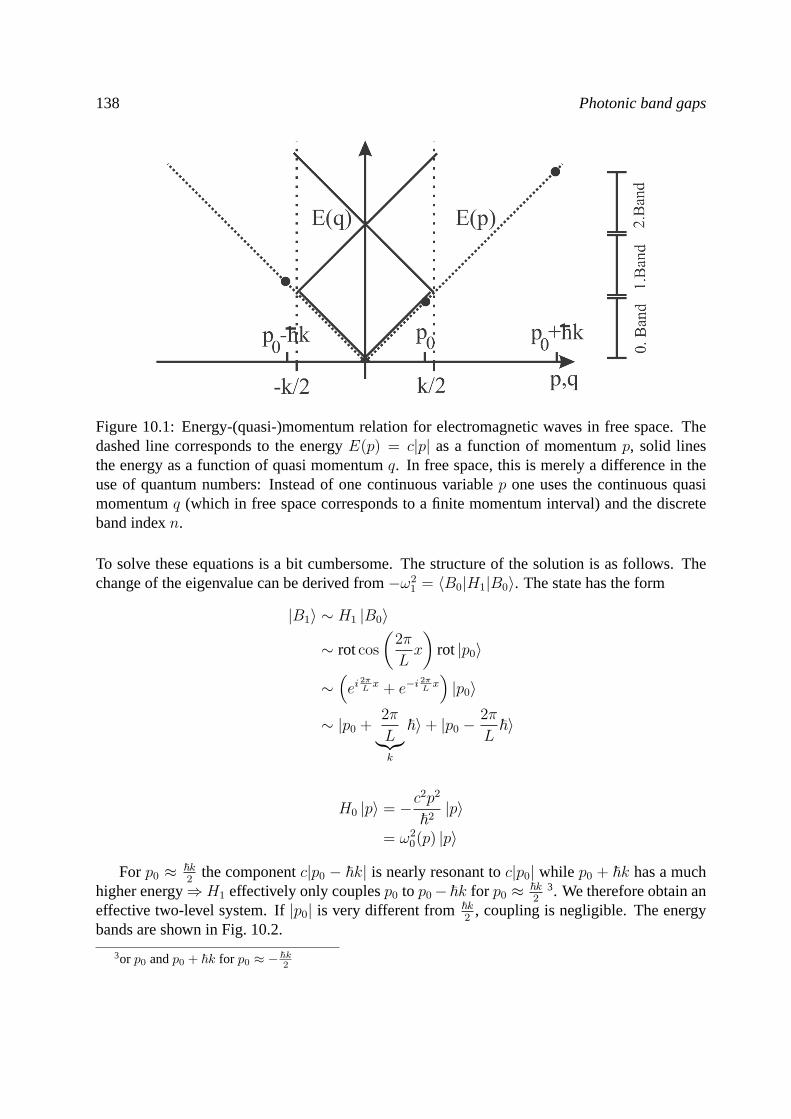
138 Photonic band gaps
Figure 10.1: Energy-(quasi-)momentum relation for electromagnetic waves in free space. Thedashed line corresponds to the energyE(p) = c|p| as a function of momentump, solid linesthe energy as a function of quasi momentumq. In free space, this is merely a difference in theuse of quantum numbers: Instead of one continuous variablep one uses the continuous quasimomentumq (which in free space corresponds to a finite momentum interval) and the discreteband indexn.
To solve these equations is a bit cumbersome. The structure of the solution is as follows. Thechange of the eigenvalue can be derived from−ω2
1 = 〈B0|H1|B0〉. The state has the form
|B1〉 ∼ H1 |B0〉
∼ rotcos
(2π
Lx
)rot |p0〉
∼(ei
2πLx + e−i
2πLx)|p0〉
∼ |p0 +2π
L︸︷︷︸k
~〉+ |p0 −2π
L~〉
H0 |p〉 = −c2p2
~2|p〉
= ω20(p) |p〉
For p0 ≈ ~k2
the componentc|p0 − ~k| is nearly resonant toc|p0| while p0 + ~k has a muchhigher energy⇒H1 effectively only couplesp0 to p0−~k for p0 ≈ ~k
23. We therefore obtain an
effective two-level system. If|p0| is very different from~k2
, coupling is negligible. The energybands are shown in Fig. 10.2.
3or p0 andp0 + ~k for p0 ≈ −~k2
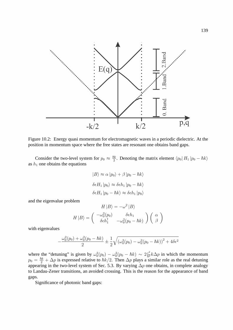
139
Figure 10.2: Energy quasi momentum for electromagnetic waves in a periodic dielectric. At theposition in momentum space where the free states are resonant one obtains band gaps.
Consider the two-level system forp0 ≈ ~k2
. Denoting the matrix element〈p0|H1 |p0 − ~k〉ash1 one obtains the equations
|B〉 ≈ α |p0〉+ β |p0 − ~k〉
δεH1 |p0〉 ≈ δεh1 |p0 − ~k〉
δεH1 |p0 − ~k〉 ≈ δεh1 |p0〉
and the eigenvalue problemH |B〉 = −ω2 |B〉
H |B〉 =
(−ω2
0(p0) δεh1
δεh†1 −ω20(p0 − ~k)
)(αβ
)with eigenvalues
−ω20(p0) + ω2
0(p0 − ~k)2
± 1
2
√(ω2
0(p0)− ω20(p0 − ~k))2
+ 4δε2
where the “detuning” is given byω20(p0) − ω2
0(p0 − ~k) ∼ 2 c2
~2k∆p in which the momentump0 = ~k
2+ ∆p is expressed relative to~k/2. Then∆p plays a similar role as the real detuning
appearing in the two-level system of Sec. 5.3. By varying∆p one obtains, in complete analogyto Landau-Zener transitions, an avoided crossing. This is the reason for the appearance of bandgaps.
Significance of photonic band gaps:
140 Photonic band gaps
• Light with frequency inside a band gap cannot propagate through the medium. This canbe used for mirrors, glass fibres, filters, . . .
• Theoretical predictions: spontaneous emission of atoms placed in the periodic mediumwill be strongly modified [22]. However, photonic crystals with band gaps stretching overthe entire angular range of photon momenta have only been produced recently [23].
Chapter 11
Bose-Einstein-Kondensate
11.1 Vielteilchentheorie bosonischer Atome
In Kapitel 2 wurde die allgemeine Struktur von Vielteilchentheorien in der Quantenmechanikbehandelt. Diese soll nun auf bosonische Atome angewendet werden:
SeiH0(x, p) ein Ein-Teilchen-Operator, z.B.
H0(x, p) =p2
2M+ V (r)
mit EigenzustandenH0ψn(x) = Enψn(x). Die Eigenzustande sollen normiert sein,〈ψn|ψm〉 =δn,m =
∫d3x ψ∗n(x)ψm(x). Mit Hilfe dieser Basis kann man den Feldoperator
Ψ(x) =∑n
anψn(x)
einfuhren, der ein Atom am Ortx vernichtet. Der Feldoperator und die Erzeuger/Vernichtererfullen die Kommutator-Relationen
[Ψ(x), Ψ†(y)] = δ(x− y) , [an, a†m] = δn,m
Freier Hamilton Operator mittels Feldoperatoren ausgedruckt:
H0 =
∫d3x Ψ†(x)H0(x,p)Ψ(x) (11.1)
wobei:p → i~∇Die Wechselwirkung wirduber einen Mehrteilchenoperator vermittelt. Der eine Kollision ver-mittelnde Operator lautet
HColl =1
2
∫d3x d3y Ψ†(x)Ψ†(y)V (x− y)Ψ(y)Ψ(x) (11.2)
Diese Darstellung des Operators im Fock”=Raum ist eine Art”Matrixelement“ des Operators
fur zwei Teilchen.V kann zum Beispiel das Coulomb Potential darstellen. Allgemein tritt proan der Wechselwirkung beteiligtem Teichen ein Feldoperator und der entsprechende adjungierteOperator (am selben Ort genommen) im Wechselwirkungs-Hamiltonian auf. Diese Darstellungder Wechselwirkung hangt eng mit den Feynman Diagrammen zusammen.
142 Bose-Einstein-Kondensate
Beispiel: Anwendung auf einen 2”=Teilchen”=Zustand
|ψ〉 = a†1a†2 |0〉d.h. 1 Teilchen in Mode 1 (11.3)
1 Teilchen in Mode 2
Der Effekt der Wechselwirkung kann nun berechnet werden. In|ψ〉 sind die beiden Atomeunkorreliert, die Wechselwirkung wird im allgemeinen ein Korrelation erzeugen. Also:
HColl |ψ〉 =1
2
∫d3x d3y Ψ†(x)Ψ†(y)V (x− y)[Ψ(y)Ψ(x), a†1a
†2] |0〉 (11.4)
dies gilt wegen
Ψ(x) |0〉 = 0 und [Ψ(y)Ψ(x), a†1a†2] |0〉 =
(Ψ(y)Ψ(x)a†1a
†2 − a†1a
†2Ψ(y)Ψ(x)
)|0〉 (11.5)
Es muß also noch der Kommutator in (11.5) berechnet werden. Man findet so unter Ausnutzungder Relation[AB,C] = A[B,C] + [A,C]B nach langerer Rechnung:
[Ψ(y)Ψ(x), a†1a†2] |0〉 =
1√2
(ψ1(y)ψ2(x) + ψ2(y)ψ1(x)) |0〉 (11.6)
wobei noch folgende nutzliche Relation verwendet wurde:
[Ψ(x), a†1] = [∑m
amψm(x), a†1]
=∑m
ψm(x) [am, a†1]︸ ︷︷ ︸
δ1m
= ψ1(x) (11.7)
Mit diesem Ergebnis erhalt man fur den Wechselwirkungshamiltonian:
HColl |Ψ〉 =
∫d3x d3y Ψ†(x)Ψ†(y)V (x− y)(ψ1(y)ψ2(x) + ψ1(x)ψ2(y)) |0〉 (11.8)
d. h. die Wirkung des Operators auf einen Zweiteilchenzustand erzeugt einen neuen Zweit-eilchenzustand, der mit dem Wechselwirkungspotential gewichtet wird und so Korrelationenzwischen Teilchen am Ortx undy enthalt.
Wechselwirkung mit Licht In diesem Fall hat der Wechselwirkungs”=Hamiltonian die Form
−d · E(x) → −∫d3x Ψ†e(x)Ψg(x)deg · E
(+)(x) + h.c. (11.9)
Wobei Ψg und Ψe jeweils Atome in Grund”= und angeregtem Zustand vernichten. Insgesamtwird also ein Photon vernichtet und ein Grundzustandsatom durch ein angeregtes ersetzt. Auchdieser Operator hat die Struktur einer Art
”Matrixelement“.
11.2 Der Bose”=Einstein”=Phasenubergang 143
Bewegungsgleichungen Im Heisenbergbild lauten die Bewegungsgleichungen eines solchenSystems:
i~ ˙Ψ = [Ψ(x), H] (11.10)
Fur den freien Anteil des Hamiltonians lauten sie insbesondere:
[Ψ(x), H0] =
∫d3x′ [Ψ(x), Ψ†(x′)H0(x
′,p′)Ψ(x′)]
=
∫d3x′ δ(x− x′)H0(x
′,p′)Ψ(x′)
= H0(x,p)Ψ(x) ≡ Schrodingergleichung (11.11)
Wahle alsψn(x) die Eigenfunktionen vonH0(x,p): H0(x,p)ψn(x) = Enψn(x):
H0(x,p)Ψ(x) =∑n
H0(x,p)anψn(x) =∑n
anEnψn(x) (11.12)
daH0 nur aufψn(x) wirkt. Damit findet man die Bewegungsgleichung
i~ ˙Ψ(x) = i~
∑n
˙anψn(x) = H0(x,p)Ψ(x) =∑n
anEnψn(x) (11.13)
⇒ an(t) = e−iEnt/~an(0) da dieψn orthogonal sind. (11.14)
Insbesondere gilt auch:
H0 =
∫d3x Ψ†(x)H0(x,p)Ψ(x) =
∫d3x
∑n
a†nψ∗n(x)H0(x,p)
∑n′
an′ψn′(x) (11.15)
=∑n,n′
a†nan′ 〈ψn|H0(x,p)|ψn′〉1-Teilchen︸ ︷︷ ︸=En′δnn
(11.16)
=∑n
a†nanEn (11.17)
Also die bereits von den Photonen bekannte Form der Gesamtenergie.
11.2 Der Bose”=Einstein”=Phasenubergang
Anwendung des eben Gelernten auf den Bose”=Einstein”=Phasenubergang. Betrachte den Gle-ichgewichtszustand eines nicht wechselwirkenden Bose”=Gases mitN Teilchen. Aus der statis-tischen Mechanikubernehmen wir die Form der Dichtematrix
% =1
Ze−β
bH0 =1
Ze−β
Pn
bNnEn Nn := a†nan
=1
Z
∏n
e−βbNnEn =
1
Z
∏n
N∑Nn=0
e−βNnEn |Nn〉〈Nn| ⇔ Spektralzerlegung (11.18)
144 Bose-Einstein-Kondensate
mit: Z := Tr e−β bH0 und der Nebenbedingung∑
nNn = N .In Lehrbuchern wird die folgende Rechnung im allgemeinen fur die großkanonische Gesamtheit
durchgefuhrt, da dort die kombinatorischen Schwierigkeiten, die aus der Nebenbedingung∑Nn =
N entstehen, wegfallen.Wir verwenden die kanonische Gesamtheit, da wir einen sehr einfachen Fall betrachten: Nur
2 Modenψ0(x), ψ1(x) sind vorhanden.
⇒ % =1
Z
N∑N1=0
e−iβN1E1︸ ︷︷ ︸1. Mode
e−β(N−N1)E0︸ ︷︷ ︸Nebenbdg.
|(N −N1)0, N1〉〈(N −N1)0, N1| (11.19)
SetzeE0 = 0, E1 = ∆E.
⇒ % =1
Z
N∑N1=0
e−βN1∆E |(N −N1)0, N1〉〈(N −N1)0, N1| (11.20)
Damit kann die Zustandssumme sehr einfach berechnet werden:
Z = Tr e−βbH0 =
N∑N1=0
e−βN1∆E (11.21)
Setzeq := e−β∆E < 1 ⇒
Z =N∑
N1=0
qN1 =1− qN+1
1− q(11.22)
Berechne die mittlere Teilchenzahl in Mode 1 (angeregte Mode):
N1 = Tr (%N1)
=1
Z
N∑N1=0
N1qN1
=1− q
1− qN+1
q
(1− q)2
1− (N + 1)qN +NqN+1
Im Fall einer großen Anzahl von Atomen findet man
limN→∞
NqN = limN→∞
N
q−N= lim
N→∞
1
− ln qq−N= lim
N→∞
(− 1
ln q
)qN = 0 (11.23)
⇒ limN→∞
N1 =q
(1− q)<∞ (q < 1) (11.24)
D. h. es tritt ein Sattigungseffekt auf. Ab einer gewissen Anzahl von Atomen gehenalle weiterenAtome, die man hinzufugt, in den Grundzustand. Fur ein freies Gas befinden sich furT → 0 alle
11.3 Atome mit Wechselwirkung, kollektive Wellenfunktion 145
Atome im Grundzustand. In einem wechselwirkenden (realen) Gas verbleibt ein Rest angeregterAtome.
Addiert man also bei festgehaltener Temperatur Teilchen zu einem bosonischen Gas, sogehen ab einer gewissen Anzahl alle neuen Teilchen in den Grundzustand. Die Anzahl der an-geregten Atome wird gesattigt.Dieses Ergebnis ist unabhangig von der Anzahl der Moden (gilt auch fur kontinuierliche Moden)und von der zu Grunde gelegten Gesamtheit (kanonisch, großkanonisch). Es existiert eine kritis-che Temperatur fur die gilt:
N0
N=N − N1
N= 1− q
N(1− q)3. 1 (11.25)
Fur kleinesβ∆E gilt nun1− q ≈ β∆E (wegenq = e−β∆E) also:
N0
N≈ 1
N(β∆E)≈ 1 (11.26)
Dies ist eine Bedingung anβ, die angibt, wann sich eine makroskopische Anzahl von Atomenim Grundzustand befindet. Bis auf numerische Vorfaktoren stimmt dies mit dem Ergebnis furharmonische Fallenuberein [25]. Im freien Raum erhalt man andere Bedingungen, die meist mitHilfe der thermischen deBroglie”=Wellenlange ausgedruckt werden:
%λ3dB = ζ
(3
2
)≈ 2.612 (11.27)
mit λdB :=√
2π~2/(MkBT ). Dies laßt sich folgendermaßen deuten: In einem thermischenGas kann man sich vorstellen, da”s die Teilchen Wellenpakete mit AusdehnungλdB bilden. DieBedingung (11.27) fur die Bose-Einstein-Kondensation bedeutet, daß man in etwa ein Teilchenpro Volumenλ3
dB hat. Hat man weniger Teilchen, souberlappen die Wellenpakete sich nicht undmerken nichts von ihrer bosonischen Natur.Uberlappen sie, so kommt es zu Beeinflussungenund die Atome kondensieren.
11.3 Atome mit Wechselwirkung, kollektive Wellenfunktion
Wechselwirkung ist fur ein BEC zwar nicht notwendig, muss aber in der Regel berucksichtigtwerden. Dies kann man durch den Hamilton-Operator
H =
∫d3x Ψ†(x)H0(x, p) Ψ(x) +
1
2
∫∫d3x d3y Ψ†(x)Ψ†(y)V (x− y) Ψ(y)Ψ(x) (11.28)
ausdrucken. Atomare BECs (87Ru,23Na, . . . ) sind verdunnte Gase in dem Sinn, dass der mittlereAbstand der Atome weit großer ist als die Streulangea ihrer Wechselwirkung1
%a3 1 (% =Dichte) (11.29)
1Die Streulangea ist definiertuber den Streuquerschnitt,σ ∝ a2. Fur dieublichen atomaren BECs ist sie einigeNanometer groß.
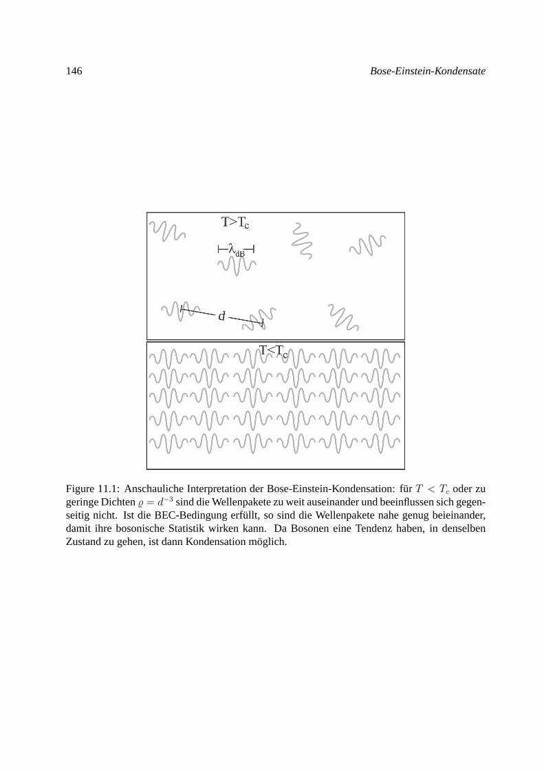
146 Bose-Einstein-Kondensate
Figure 11.1: Anschauliche Interpretation der Bose-Einstein-Kondensation: fur T < Tc oder zugeringe Dichten% = d−3 sind die Wellenpakete zu weit auseinander und beeinflussen sich gegen-seitig nicht. Ist die BEC-Bedingung erfullt, so sind die Wellenpakete nahe genug beieinander,damit ihre bosonische Statistik wirken kann. Da Bosonen eine Tendenz haben, in denselbenZustand zu gehen, ist dann Kondensation moglich.
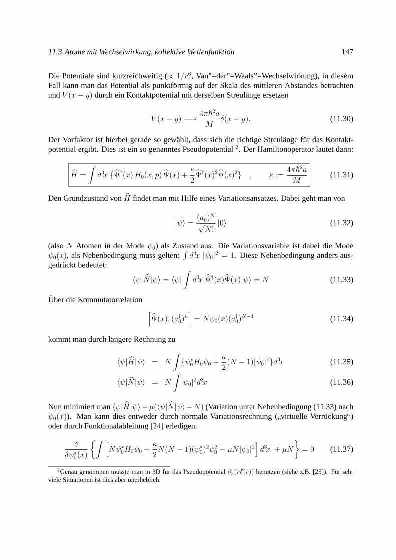
11.3 Atome mit Wechselwirkung, kollektive Wellenfunktion 147
Die Potentiale sind kurzreichweitig (∝ 1/r6, Van”=der”=Waals”=Wechselwirkung), in diesemFall kann man das Potential als punktformig auf der Skala des mittleren Abstandes betrachtenundV (x− y) durch ein Kontaktpotential mit derselben Streulange ersetzen
V (x− y) −→ 4π~2a
Mδ(x− y). (11.30)
Der Vorfaktor ist hierbei gerade so gewahlt, dass sich die richtige Streulange fur das Kontakt-potential ergibt. Dies ist ein so genanntes Pseudopotential2. Der Hamiltonoperator lautet dann:
H =
∫d3x Ψ†(x)H0(x, p) Ψ(x) +
κ
2Ψ†(x)2Ψ(x)2 , κ :=
4π~2a
M(11.31)
Den Grundzustand vonH findet man mit Hilfe eines Variationsansatzes. Dabei geht man von
|ψ〉 =(a†0)
N
√N !
|0〉 (11.32)
(alsoN Atomen in der Modeψ0) als Zustand aus. Die Variationsvariable ist dabei die Modeψ0(x), als Nebenbedingung muss gelten:
∫d3x |ψ0|2 = 1. Diese Nebenbedingung anders aus-
gedruckt bedeutet:
〈ψ|N |ψ〉 = 〈ψ|∫d3x Ψ†(x)Ψ(x)|ψ〉 = N (11.33)
Uber die Kommutatorrelation[Ψ(x), (a†0)
n]
= Nψ0(x)(a†0)N−1 (11.34)
kommt man durch langere Rechnung zu
〈ψ|H|ψ〉 = N
∫ψ∗0H0ψ0 +
κ
2(N − 1)|ψ0|4d3x (11.35)
〈ψ|N |ψ〉 = N
∫|ψ0|2d3x (11.36)
Nun minimiert man〈ψ|H|ψ〉−µ(〈ψ|N |ψ〉−N) (Variation unter Nebenbedingung (11.33) nachψ0(x)). Man kann dies entweder durch normale Variationsrechnung (
”virtuelle Verruckung“)
oder durch Funktionalableitung [24] erledigen.
δ
δψ∗0(x)
∫ [Nψ∗0H0ψ0 +
κ
2N(N − 1)(ψ∗0)
2ψ20 − µN |ψ0|2
]d3x + µN
= 0 (11.37)
2Genau genommen musste man in 3D fur das Pseudopotential∂r(rδ(r)) benutzen (siehe z.B. [25]). Fur sehrviele Situationen ist dies aber unerheblich.
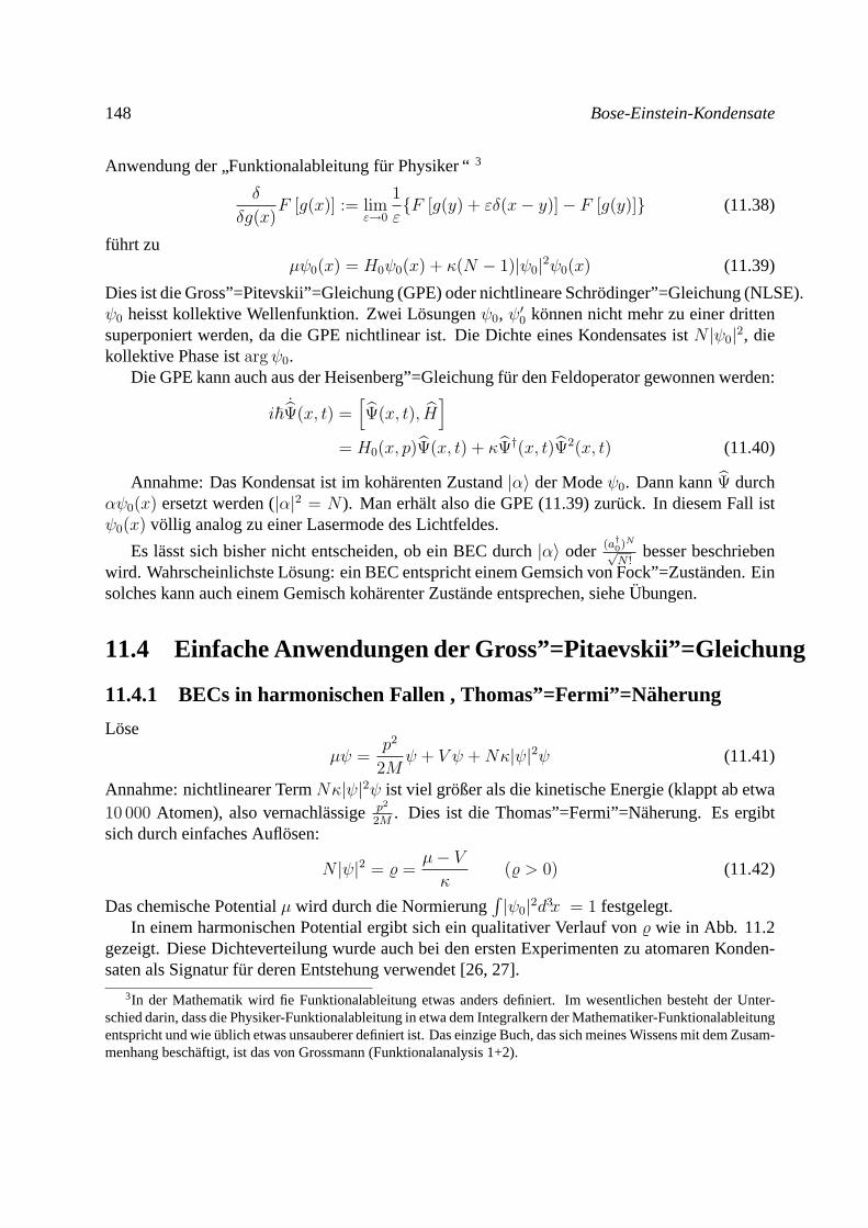
148 Bose-Einstein-Kondensate
Anwendung der”Funktionalableitung fur Physiker “3
δ
δg(x)F [g(x)] := lim
ε→0
1
εF [g(y) + εδ(x− y)]− F [g(y)] (11.38)
fuhrt zuµψ0(x) = H0ψ0(x) + κ(N − 1)|ψ0|2ψ0(x) (11.39)
Dies ist die Gross”=Pitevskii”=Gleichung (GPE) oder nichtlineare Schrodinger”=Gleichung (NLSE).ψ0 heisst kollektive Wellenfunktion. Zwei Losungenψ0, ψ′0 konnen nicht mehr zu einer drittensuperponiert werden, da die GPE nichtlinear ist. Die Dichte eines Kondensates istN |ψ0|2, diekollektive Phase istargψ0.
Die GPE kann auch aus der Heisenberg”=Gleichung fur den Feldoperator gewonnen werden:
i~ ˙Ψ(x, t) =
[Ψ(x, t), H
]= H0(x, p)Ψ(x, t) + κΨ†(x, t)Ψ2(x, t) (11.40)
Annahme: Das Kondensat ist im koharenten Zustand|α〉 der Modeψ0. Dann kannΨ durchαψ0(x) ersetzt werden (|α|2 = N ). Man erhalt also die GPE (11.39) zuruck. In diesem Fall istψ0(x) vollig analog zu einer Lasermode des Lichtfeldes.
Es lasst sich bisher nicht entscheiden, ob ein BEC durch|α〉 oder (a†0)N
√N !
besser beschriebenwird. Wahrscheinlichste Losung: ein BEC entspricht einem Gemsich von Fock”=Zustanden. Einsolches kann auch einem Gemisch koharenter Zustande entsprechen, sieheUbungen.
11.4 Einfache Anwendungen der Gross”=Pitaevskii”=Gleichung
11.4.1 BECs in harmonischen Fallen , Thomas”=Fermi”=Naherung
Lose
µψ =p2
2Mψ + V ψ +Nκ|ψ|2ψ (11.41)
Annahme: nichtlinearer TermNκ|ψ|2ψ ist viel großer als die kinetische Energie (klappt ab etwa10 000 Atomen), also vernachlassige p2
2M. Dies ist die Thomas”=Fermi”=Naherung. Es ergibt
sich durch einfaches Auflosen:
N |ψ|2 = % =µ− V
κ(% > 0) (11.42)
Das chemische Potentialµ wird durch die Normierung∫|ψ0|2d3x = 1 festgelegt.
In einem harmonischen Potential ergibt sich ein qualitativer Verlauf von% wie in Abb. 11.2gezeigt. Diese Dichteverteilung wurde auch bei den ersten Experimenten zu atomaren Konden-saten als Signatur fur deren Entstehung verwendet [26, 27].
3In der Mathematik wird fie Funktionalableitung etwas anders definiert. Im wesentlichen besteht der Unter-schied darin, dass die Physiker-Funktionalableitung in etwa dem Integralkern der Mathematiker-Funktionalableitungentspricht und wieublich etwas unsauberer definiert ist. Das einzige Buch, das sich meines Wissens mit dem Zusam-menhang beschaftigt, ist das von Grossmann (Funktionalanalysis 1+2).
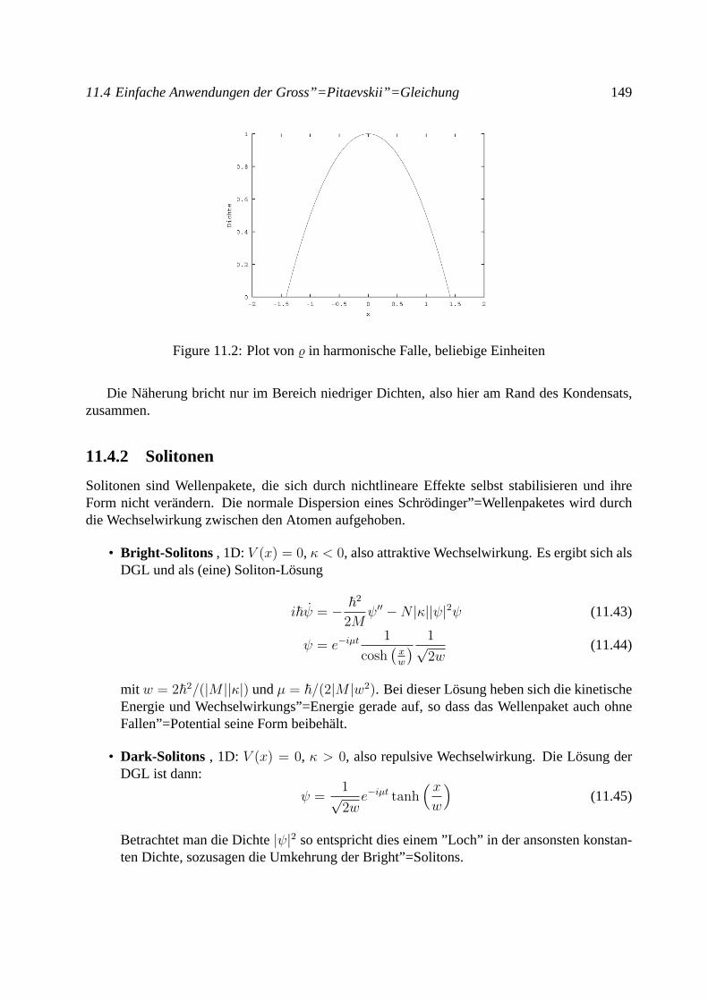
11.4 Einfache Anwendungen der Gross”=Pitaevskii”=Gleichung 149
Figure 11.2: Plot von% in harmonische Falle, beliebige Einheiten
Die Naherung bricht nur im Bereich niedriger Dichten, also hier am Rand des Kondensats,zusammen.
11.4.2 Solitonen
Solitonen sind Wellenpakete, die sich durch nichtlineare Effekte selbst stabilisieren und ihreForm nicht verandern. Die normale Dispersion eines Schrodinger”=Wellenpaketes wird durchdie Wechselwirkung zwischen den Atomen aufgehoben.
• Bright-Solitons , 1D:V (x) = 0, κ < 0, also attraktive Wechselwirkung. Es ergibt sich alsDGL und als (eine) Soliton-Losung
i~ψ = − ~2
2Mψ′′ −N |κ||ψ|2ψ (11.43)
ψ = e−iµt1
cosh(xw
) 1√2w
(11.44)
mit w = 2~2/(|M ||κ|) undµ = ~/(2|M |w2). Bei dieser Losung heben sich die kinetischeEnergie und Wechselwirkungs”=Energie gerade auf, so dass das Wellenpaket auch ohneFallen”=Potential seine Form beibehalt.
• Dark-Solitons , 1D: V (x) = 0, κ > 0, also repulsive Wechselwirkung. Die Losung derDGL ist dann:
ψ =1√2w
e−iµt tanh( xw
)(11.45)
Betrachtet man die Dichte|ψ|2 so entspricht dies einem ”Loch” in der ansonsten konstan-ten Dichte, sozusagen die Umkehrung der Bright”=Solitons.
150 Bose-Einstein-Kondensate
• Gap-Solitonssind Bright”=Solitons fur sich abstoßende (κ > 0) Atome. In diesem Fallist die nichtlineare Energie positiv. Die Idee ist, dass man zur Kompensation die kinetischeEnergie mit Hilfe von Bandlucken negativ macht. Im periodischen Potential hat die freieEnergie freier Teilchen eine Bandstruktur.
An der oberen Bandkante gilt:E0(q) ≈ E0− ~2|M∗|(q−
k2)2. M∗ < 0 heißt effektive Masse
(= inverse der Krummung vonE0(q))
Entwickelt manψ nach Bloch”=Funktionen um die obere Bandkante herum, so kann manp2
2M+ V (x) durchE0(q) ersetzen und erhalt eine effektive negative kinetische Energie, die
sich gegen die positive nichtlineare Energie aufheben kann.
Chapter 12
Appendices
12.1 Green’s function
Consider a general linear inhomogeneous differential equation (DEQ) of the form
(LxF )(x) = h(x)
A Green’s function is a special solution with the inhomogeneityδ (x− x′).
(LxG)(x,x′) = δ (x− x′)
If one knowsG (x,x′), the solution of the general inhomogeneous DEQ is given by
F (x) =
∫G(x,x′) · h(x′) dx′ (12.1)
Proof:
(LxF )(x) = Lx
∫dx′G(x, x′) · h(x)
=
∫dx′ LxG(x, x′) · h(x)
=
∫dx′ δ (x− x′)h(x) = h(x)
12.2 Angular momentum algebra
At the beginning a word of caution: in angular momentum algebra different conventions areused in different textbooks, which are distinguished by their choice of phases of the angularmomentum eigenstates. We follow the convention of Ref. [4], which also seems to be used inthe Mathematica software package. Other good references on angular momentum in quantumphysics are Refs. [2] und [3].
152 Appendices
Angular momentum is defined as a vectorL whose three components are operators fulfillingthe commutation relations
[La,Lb] = i~εabcLc . (12.2)
It can be shown that[L2,Li] = 0 ist. Hence, one can find a common set of eigenstates ofL2 andone of the components, which usually is chosen to beLz:
L2|l,m〉 = ~2l(l + 1)|l,m〉 , Lz|l,m〉 = ~m|l,m〉 (12.3)
Here,m runs from−l to l andl = 0, 1/2, 1, . . ..It is advantageous to introduce the operatorsL± := Lx±iLy, which obey[L±,Lz] = ∓~L±
and[L+,L−] = 2~Lz. It follows that
∓ ~L±|l,m〉 = [L±,Lz]|l,m〉= m~L±|l,m〉 −LzL±|l,m〉 (12.4)
Hence,L±|l,m〉 is proportional to|l,m± 1〉. SinceL†+ = L− andL2 = L2z +L−L+ + ~Lz we
find
〈l,m|L2|l,m〉 = ~2l(l + 1)
= 〈l,m|L2z + L−L+ + ~Lz|l,m〉
= ~2m2 + ~2m+ |〈l,m+ 1|L+|l,m〉|2 (12.5)
and thus
〈l′,m′|L+|l,m〉 = 〈l,m|L−|l′,m′〉 = ~fl,m δl,l′ δm+1,m′ (12.6)
The phase factors of the states|l,m〉 can be chosen in such a way that the matrix elements arereal. We have introduced the notation
fl,m :=√l(l + 1)−m(m+ 1) (12.7)
since this factor appears frequently. A very useful consequence of Eq. (12.6) is that for a givenlall the states|l,m〉 can be obtained from|l,−l〉 by repeated application of the operatorJ+.
12.2.1 Addition of two angular momenta
When adding two (commuting) angular momentum operatorsL andS to J = L+S, one has toaddress the question of choosing a suitable basis for the product of the respective Hilbert spaces.A possible choice would obviously be the tensor product of the individual bases,
|l,ml; s,ms〉 := |l,ml〉 ⊗ |s,ms〉 . (12.8)
However, it is usually more convenient to work with eigenstates ofJ2 andJ z instead. Because[L2,J i] = [S2,J i] = 0 these states are characterized by four quantum numbers
|j,mj, (l, s)〉 . (12.9)
12.2 Angular momentum algebra 153
The matrix elements〈l,ml; s,ms|j,mj, (l, s)〉 =: 〈l,ml; s,ms|j,mj〉 are calledClebsch-Gordancoefficientsand allow to switch from one basis to the other:
|j,mj, (l, s)〉 =∑ml,ms
〈l,ml; s,ms|j,mj, 〉 |l,ml; s,ms〉 (12.10)
By applying J z one can easily see thatms + ml = mj is valid. The numerical values forClebsch-Gordan coefficients can be derived from the linear system of equations
〈l,ml; s,ms|J+|j,mj, (l, s)〉 = ~fj,mj〈l,ml; s,ms|j,mj + 1〉 (12.11)
= 〈l,ml; s,ms|(L+ + S+)|j,mj, (l, s)〉= 〈j,mj, (l, s)|(L− + S−)|l,ml; s,ms〉∗
= ~fl,ml−1〈l,ml − 1; s,ms|j,mj〉+~fs,ms−1〈l,ml; s,ms − 1|j,mj〉
and the analogous equation forJ−,
fj,mj−1〈l,ml; s,ms|j,mj − 1, 〉 = fl,ml〈l,ml + 1; s,ms|j,mj〉 (12.12)
+fs,ms〈l,ml; s,ms + 1|j,mj〉 ,
as well as the normalization condition
1 = 〈j,mj, (l, s)|j,mj, (l, s)〉=
∑ml,ms
|〈l,ml; s,ms|j,mj〉|2 . (12.13)
Generally, Clebsch-Gordan coefficients are only non-zero forl + s ≥ j ≥ |l − s|. In theliterature one also finds Wigner’s3j-symbol instead of Clebsch-Gordan coefficients, to whichthey are related by(
l s jml ms −mj
):=
(−1)l−s+mj
√2j + 1
〈l,ml; s,ms|j,mj〉 . (12.14)
Wigner’s3j-symbol is more symmetric than Clebsch-Gordan coefficients. It is invariant undercyclic permutations of the three columns. Under an anti-cyclic permutation, or under simultane-ous change of the sign ofml,ms andmj, it obtains a factor of(−1)l+s+j.
12.2.2 Tensor operators and Wigner-Eckart theorem
Tensor operatorsTk,mkare defined by their transformation properties under rotations. They cor-
respond to an irreducible representation of the rotation group. Equivalently, they can be definedas operators which fulfill the following commutation relations with a given angular momentumoperatorJ ,
[Jz, Tk,mk] = ~mkTk,mk
(12.15)
[J+, Tk,mk] = ~fk,mk
Tk,mk+1 (12.16)
[J−, Tk,mk] = ~fk,mk−1Tk,mk−1 . (12.17)
154 Appendices
Tensor operators are of great importance for atomic selection rules and allow an elegant deriva-tion of the latter by means of the Wigner-Eckart theorem.
To prove the Wigner-Eckart theorem we first consider the states
˜|j′′,m′′j (j, k)〉 :=∑mk,mj
〈j′′,m′′j |j,mj; k,mk〉 Tk,mk|j,mj〉 (12.18)
The action ofJz on these states is given by
Jz ˜|j′′,m′′j (j, k)〉 =∑mk,mj
〈j′′,m′′j |j,mj; k,mk〉 ×
([Jz, Tk,mk] + Tk,mk
Jz)|j,mj〉=
∑mk,mj
〈j′′,m′′j |j,mj; k,mk〉 ×
(~mkTk,mk+ Tk,mk
~mj)|j,mj〉
= ~m′′j ˜|j′′,m′′j (j, k)〉 (12.19)
where the last step follows from the fact that Clebsch-Gordan coefficients are non-zero only formk +mj = m′′j . The action ofJ+ reads
J+˜|j′′,m′′j (j, k)〉 =
∑mk,mj
〈j′′,m′′j |j,mj; k,mk〉 ([J+, Tk,mk] + Tk,mk
J+)|j,mj〉
=∑mk,mj
〈j′′,m′′j |j,mj; k,mk〉 ×~fk,mkTk,mk + 1︸ ︷︷ ︸
=m′k
|j,mj〉+ Tk,mk~fj,mj
|j,mj + 1︸ ︷︷ ︸=m′
j
〉
= ~
∑mk,mj
〈j′′,m′′j |j,mj; k,mk − 1〉 fk,mk−1 Tk,mk|j,mj〉
+~∑mk,mj
〈j′′,m′′j |j,mj − 1; k,mk〉 fj,mj−1 Tk,mk|j,mj〉
= ~∑mk,mj
(〈j′′,m′′j |j,mj; k,mk − 1〉 fk,mk−1
+〈j′′,m′′j |j,mj − 1; k,mk〉 fj,mj−1
)Tk,mk
|j,mj〉
= ~∑mk,mj
fj′′,m′′j〈j′′,m′′j + 1|j,mj; k,mk〉 Tk,mk
|j,mj〉
= ~fj′′,m′′j
˜|j′′,m′′j + 1(j, k)〉 (12.20)
where we have used Eq. (12.12) in the second-to-last step. Analogously, we find forJ−
J− ˜|j′′,m′′j (j, k)〉 = ~fj′′,m′′j−1
˜|j′′,m′′j − 1(j, k)〉 (12.21)
12.2 Angular momentum algebra 155
The action of the angular momentum operators on the states|j′′,m′′j (j, k)〉 is the same as on theangular momentum eigenstates|j′′,m′′j 〉. Therefore, these states need to be proportional to eachother. Since for givenj′′ the eigenstates|j′′,m′′j 〉 can be constructed by applyingJ+ to |j′′,−j′′〉,this can also be done for the states ˜|j′′,m′′j (j, k)〉. For this reason, the proportionality factorbetween the states is independent fromm′′j and we find
˜|j′′,m′′j (j, k)〉 = (−1)2k 〈j′′||Tk||j〉√2j′′ + 1
|j′′,m′′j 〉 . (12.22)
The symbol〈j′′||Tk||j〉 is called reduced matrix element and contains the dependence of theproportionality factor onj′′, k andj. The factor of(−1)2k/
√2j′′ + 1 is convention. It is easy to
see that the reduced matrix element can be calculated by
〈j′′||Tk||j〉 = (−1)2k√
2j′′ + 1∑mk,mj
〈j′′,m′′j |j,mj; k,mk〉〈j′′,m′′j |Tk,mk|j,mj〉 (12.23)
The matrix elements of tensor operators can be derived from Eq. (12.22). Because of thecompleteness of the angular momentum eigenstates we have∑
j′′,m′′j
〈j,mj; k,mk|j′′,m′′j 〉 ˜|j′′,m′′j (j, k)〉 =∑j′′,m′′
j
〈j,mj; k,mk|j′′,m′′j 〉 ×∑m′
k,m′j
〈j′′,m′′j |j,m′j; k,m′k〉 Tk,m′k|j,m′j〉
=∑m′
k,m′j
〈j,mj; k,mk|j,m′j; k,m′k〉 Tk,m′k|j,m′j〉
= Tk,mk|j,mj〉 (12.24)
and thus
〈j′,m′j|Tk,mk|j,mj〉 =
∑j′′,m′′
j
〈j,mj; k,mk|j′′,m′′j 〉〈j′,m′j ˜|j′′,m′′j (j, k)〉
= (−1)2k 〈j′||Tk||j〉√2j′ + 1
〈j,mj; k,mk|j′,m′j〉 (12.25)
This is the Wigner-Eckart theorem.
12.2.3 Addition of three angular momenta
When adding three or more angular momenta one has to be careful with the choice of basis.Consider the caseF = I + L + S. If we first addJ = S + L and thenF = I + J ,the procedure of the previous section would result in the basis states|f,mf , (i, j(s, l))〉, i.e.,eigenstates ofF 2, F z, I
2, andJ2. However, if we first addΣ = I +S and thenF = Σ+L, we
156 Appendices
implicitly would use the basis|f,mf , (σ(i, s), l)〉. The two sets of basis vectors are different.In a sense the addition of angular momenta is therefore not associative (although the addition ofthe operators is of course associative). Which of the two bases is more suitable depends entirelyon the physical situation at hand.
Detailed construction of the basis states:
|f,mf , (i, j(s, l))〉 =∑mi,mj
〈i,mi; j,mj|f,mf〉 |i,mi〉 ⊗ |j,mj(s, l)〉
=∑mi,mj
〈i,mi; j,mj|f,mf〉 ×∑ms,ml
〈s,ms; l,ml|j,mj〉 |i,mi〉 ⊗ |s,ms〉 ⊗ |l,ml〉 (12.26)
|f,mf , (σ(i, s), l)〉 =∑mσ ,ml
〈σ,mσ; l,ml|f,mf〉 |σ,mσ(i, s)〉 ⊗ |l,ml〉
=∑mσ ,ml
〈σ,mσ; l,ml|f,mf〉 ×∑mi,ms
〈i,mi; s,ms|σ,mσ〉 |i,mi〉 ⊗ |s,ms〉 ⊗ |l,ml〉 (12.27)
Multiplication of the vectors results in
〈f,mf , (i, j(s, l))|f ′,m′f , (σ(i, s), l)〉 =∑
mj,mσmi,ml,ms
〈i,mi; j,mj|f,mf〉 〈σ,mσ; l,ml|f ′,m′f〉
〈s,ms; l,ml|j,mj〉 〈i,mi; s,ms|σ,mσ〉= (2f + 1)
√(2j + 1)(2σ + 1)
∑mj,mσ
mi,ml,ms
(−1)2i−j−2l+σ+2mf+mj+mσ
(i j fmi mj −mf
)(σ l f ′
mσ ml −m′f
)(
s l jms ml −mj
)(i s σmi ms −mσ
)=: δf,f ′δmf ,m
′f
√(2j + 1)(2σ + 1)×
(−1)i+s+l+fi s σl f j
(12.28)
The last line defines Wigner’s6j-Symbol, which agrees with the so-called Racah symbolsW (· · · )up to a sign:
i s σl f j
= (−1)i+s+l+fW (i, s, l, f ;σ, j) . (12.29)
The expression for the6j-Symbol as a sum over Clebsch-Gordan coefficients is equivalent toEq. (C.32) of Ref. [4].
12.2 Angular momentum algebra 157
12.2.4 Matrix elements for composed systems
The content of this section is of great importance for the actual calculation of multipole ma-trix elements for atoms and molecules. One often has to resolve the problem that the atomicenergy eigenstates are (to a good approximation) eigenstates of the hyperfine-spin operatorF , but the dipole matrix elements have to be calculated with respect to the electronic statesalone (without nuclear spinI). Generally one needs to express the reduced matrix element〈f ′(i′, j′)||T (j)
k ||f(i, j)〉 of a tensor operatorT (j)k,mk
, that only acts on the total electronic angular
momentumJ , through〈j′||T (j)k ||j〉.
To achieve this one starts from Eq. (12.23) and expands, with the aid of Eq. (12.10), thehyperfine states|f,mf〉 in terms of the nuclear spin eigenstates|i,mi〉 and the eigenstates|j,mj〉of te total electronic angular momentum. One then arrives at
〈f ′(i′, j′)||T (j)k ||f(i, j)〉 = (−1)2k
√2f ′ + 1
∑mk,mf
〈f ′,m′f |f,mf ; k,mk〉〈f ′,m′f |T(j)k,mk
|f,mf〉
= (−1)2k√
2f ′ + 1∑mk,mf
∑mi,mj
∑m′
i,m′j
〈f ′,m′f |f,mf ; k,mk〉〈f ′,m′f |i′,m′i; j′,m′j〉 ×
〈i,mi; j,mj|f,mf〉〈i′,m′i, j′,m′j|T(j)k,mk
|i,mi, j,mj〉
= (−1)2k√
2f ′ + 1∑mk,mf
∑mi,mj
∑m′
i,m′j
〈f ′,m′f |f,mf ; k,mk〉〈f ′,m′f |i′,m′i; j′,m′j〉 ×
δi,i′δmi,m′i〈i,mi; j,mj|f,mf〉〈j′,m′j|T
(j)k,mk
|j,mj〉
=√
2f ′ + 1δi,i′∑
mk,mf
mi,mj ,m′j
〈f ′,m′f |f,mf ; k,mk〉〈f ′,m′f |i′,m′i; j′,m′j〉 ×
〈i,mi; j,mj|f,mf〉〈j′||T (j)
k ||j〉√2j′ + 1
〈j,mj; k,mk|j′,m′j〉
=
√2f ′ + 1
2j′ + 1δi,i′〈j′||T (j)
k ||j〉 ×∑mk,mf
mi,mj ,m′j
〈f,mf ; k,mk|f ′,m′f〉〈i,mi; j′,m′j|f ′,m′f〉 ×
〈i,mi; j,mj|f,mf〉〈j,mj; k,mk|j′,m′j〉 (12.30)
The sum in the last two lines can be written as a6j symbol by using Eq. (12.28) withf ′ =f,m′f = mf . In the sum over the Clebsch-Gordan coefficients onlymf is not a summationindex. Thereforef in Eq. (12.28) corresponds tof ′ in Eq. (12.30). All other relations can be
158 Appendices
derived from the position of the indices in the Clebsch-Gordan coefficients. One thus deducesi j fk f ′ j′
=
(−1)i+j+k+f′√
(2j′ + 1)(2f + 1)
∑m′
j,mf
mi,mk,mj
〈i,mi; j′,m′j|f ′,m′f〉 〈f,mf ; k,mk|f ′,m′f〉
〈j,mj; k,mk|j′,m′j〉 〈i,mi; j,mj|f,mf〉 (12.31)
and therefore
〈f ′(i′, j′)||T (j)k ||f(i, j)〉 =
√(2f + 1)(2f ′ + 1)δi,i′(−1)i+j+k+f
′ ×
〈j′||T (j)k ||j〉
i j fk f ′ j′
(12.32)
This is equivalent to Eq. (C.90) of Ref. [4].
12.3 Distributions
Distributions are mathematical objects which, strictly speaking, are only defined if they appearin an integral. For instance,δ(x− x0) is only defined through its effect inside the integral∫
dx f(x)δ(x− x0) := f(x0)
Here,f(x) is a so-called Test function. These are functions which, speaking in a sloppy way,“always behave well”. More formally, they areC∞ functions with compact support, or at leastthey converge sufficiently fast to zero for|x| −→ ∞). Distributions are no functions. Forexample,δ(x− x0) is not well defined as a function at the positionx0.
The integralD(ω) :=∫∞
0dτ e−iωτ is also only defined in the sense of distributions:∫ ∞
−∞dω D(ω)f(ω) =
∫ ∞−∞
dω f(ω)
∫ ∞0
dτ e−iωτ
=
∫ ∞−∞
dω f(ω)(πδ(ω)− iP c
ω)
= πf(0)− i limε→0+
(
∫ −ε−∞
dω
ωf(ω) +
∫ ∞ε
dω
ωf(ω))
The transition from the first to the second line relies on a mathematical theorem. The principalvalue in this expression means that one has to use the same small parameterε on both sides of thesingularity of the integrand. If one calculates the limiting value of an integral without principalvalue, one has to admit different small parameters on both sides of the singularity.
Bibliography
[1] J.D. Jackson,Classical Electrodynamics, Wiley 1999.
[2] J.J. Sakurai,Modern Quantum Mechanics, Addison Wesley, 1994.
[3] D.M. Brink and G.R. Satchler,Angular Momentum, Oxford Library of Physical Sciences1968.
[4] A. Messiah,Quantum mechanics, Vol. 2, Wiley, New York 1963.
[5] R. F. Streater and A. S. Wightman,PCT, spin and statistics, and all that(1964) Beautifultext on the axiomatic formulation of QFT, i.e., the derivation of the properties of any QFTfrom a few basic axioms (such as Einstein locality). Mathematically superb, although someconclusions of this theory are discouraging. It nevertheless provides rigorous proofs of thespin-statistics theorem (i.e, that Bosons must have integer spin) and the PCT theorem (anyQFT must be invariant under a space inversion followed by charge conjugation and timereversal).
[6] D.F. Walls und G. Milburn,Quantum Optics, Springer, Berlin (1995).
[7] P. Meystre und M. Sargent,Elements of Quantum Optics, 3. Auflage, Springer, Berlin(1999).
[8] P.W. Milonni,The quantum vacuum : an introduction to quantum electrodynamics(1994).A very interesting book which mostly deals with the effect of boundaries (Casimir effect)and some particular quantum field theoretical effects in (mostly non-relativistic) QED.
[9] J.D.Bjorken und S.D.Drell Relativistische Quantenfeldtheorie, BI-Hochschultaschenbucher 101, Mannheim (1967).
[10] E.R. Pike und S. Sarkar,The quantum theory of radiation, Clarendon Press, Oxford (1995).
[11] C. Cohen-Tannoudji, J. Dupont-Roc und G. Grynberg,Atom-photon interactions : basicprocesses and applications(1992). A very good book dealing with the fundamental tech-niques to describe the interaction of atoms with light. Includes dressed states, resolventmethod, master equations.
160 BIBLIOGRAPHY
[12] C. Cohen-Tannoudji,Atomic motion in laser light, in Fundamental systems in quantumoptics, edited by J. Dalibard, J.M. Raimond and J. Zinn-Justin, Les Houches Session LIII,Elsevier Sience Publishers 1992.
[13] J. Dalibard and C. Cohen-Tannoudji,Atomic motion in laser light: connection betweensemiclassical and quantum descriptions, J. Phys. B18, 1661 (1985).
[14] S.-Y. Zhu and M.O. Scully,Spectral Line Elimination and Spontaneous Emission Cancel-lation via Quantum Interference, Phys. Rev. Lett.76, 388 (1996).
[15] H.-R. Xia, C.-Y. Ye, and S.-Y. Zhu,Experimental observation of spontaneous emissioncancellation, Phys. Rev. Lett.77, 1032 (1996).
[16] Li Li, X. Wang, J. Yang, G. Lazarov, J. Qi, and A. M. Lyyra,Comment on ”ExperimentalObservation of Spontaneous Emission Cancellation”, Phys. Rev. Lett.84, 4016 (2000).
[17] M. Abramowitz and I.A. Stegun (Eds.),Handbook of mathematical functions, Dover, NewYork 1972.
[18] A. Galindo and P. Pascual,Quantum mechanics, Springer, Heidelberg (1990).
[19] M. Redhead,Incompleteness, nonlocality and realism : a prolegomenon to the philosophyof quantum mechanics, Oxford: Clarendon Pr., 1987.
[20] A. Aspect, E. Arimondo, R. Kaiser, N. Vansteenkiste, and C. Cohen-Tannoudji,Laser cool-ing below the one photon recoil energy by velocity-selective coherent population trapping:theoretical analysis, Journ. Opt. Soc. Am. B6, 2112 (1989).
[21] L.V. Hau., SE Harris, Z. Dutton, and C.H. Behroozi,Light speed reduction to 17 metres persecond in an ultracold atomic gas, Nature397, 594-598 (1999).
[22] S. John and T. Quang,Spontaneous emission near the edge of a photonic band gap,Phys. Rev. A50, 1764 (1994).
[23] A. Blancoet al., Nature405, 437 (2000).
[24] S. Grossmann,Funktionalanalysis, Frankfurt a.M.: Akad.Verl.ges., 1970.
[25] Y. Castin, Bose-Einstein condensates in atomic gases: simple theoretical results,http://xxx.uni-augsburg.de, cond-mat/0105058.
[26] M. Anderson, J. R. Ensher, M. R. Matthews, C. E. Wieman, and E. A. Cornell, Science269, 198 (1995).
[27] M.-O. Mewes, M. R. Andrews, N. J. van Druten, D. M. Kurn, D. S. Durfee, C. G. Townsendand W. Ketterle, Phys. Rev. Lett.77, 416 (1996).
BIBLIOGRAPHY 161
[28] E.A. Power and S. Zienau,Coulomb gauge in nonrelativistic quantum electrodynamics andthe shape of spectral lines, Phil. Trans. A251, 427 (1959).
[29] R.G. Woolley,A reformulation of molecular quantum electrodynamics, Journ. Phys. B7,488 (1974).
[30] Claude Cohen-Tannoudji, Jacques Dupont-Roc, and Gilbert Grynberg,Photons and atoms: introduction to quantum electrodynamics (1989). In this book the fundamental equationsof non-relativistic QED are thoroughly explained.
[31] D.P. Craig and T. Thirunamachandran,Molecular quantum electrodynamics : an introduc-tion to radiation-molecule interactions(1997). Despite its title it is also very useful foratoms. A cheap (15 Euro) alternative to the first book.
[32] M.O. Scully and M.S. Zubairy,Quantum Optics(1997). A very nice introduction whichalso covers electromagnetically induced transparency.
[33] Leonard Mandel and Emil Wolf,Optical coherence and quantum optics(1995). One of themost comprehensive and complete texts on quantum optics. Gives a good survey of mosttechniques and topics.
[34] D.F. Phillips, A. Fleischhauer, A. Mair, R. L. Walsworth, M. D. Lukin,Storage of Light inAtomic Vapor, Phys. Rev. Lett.86, 783 (2001).
[35] C. Liu, Z. Dutton, C.H. Behrozzi, and L.V. Hau,Observation of coherent optical informa-tion storage in an atomic medium using halted light pulses, Nature409, 490 (2001).
[36] F. Riehle, T. Kisters, A. Witte, J. Helmcke und C.J. Borde, Optical Ramsey spectroscopyin a rotating frame: Sagnac effect in a matter-wave interferometer, Phys. Rev. Lett.67,177(1991).
[37] C.J. Borde,Atomic interferometry with internal state labeling, Phys. Lett. A140, 10 (1989).
[38] M. Kasevich und S. Chu,Atomic Interferometry using stimulated Raman Transitions,Phys. Rev. Lett.67, 181 (1991).
[39] O. Carnal und J. Mlynek,Young’s Double Slit Experiment with Atoms: A Simple AtomInterferometer, Phys. Rev. Lett.66, 2689 (1991).
[40] T. Kato, J. Phys. Soc. Jap.5, 435 (1950).
[41] M.V. Berry, Proc. Roy. Soc. (Lond.)392, 45 (1984).
Index
adiabatic elemination, 83Adiabatic theorem, 84adiabatische Naherung, 123Anihilation operator, 20Atom-Interferometrie, 89avoided crossing, 74, 139
Baker-Campbell-Hausdorf equation, 32Berry phase, 85Bessel functions
spherical, 6Bewegungsgleichung
Vielteilchensystem, 143Bloch sphere, 69Bloch vector, 69Born-Oppenheimer Naherung, 123Bose-Einstein
-Ubergang, 143Kondensat, 141
Bose-Gas, 143
canonical quantisation, 44Casimir effect, 30charge conservation, 2Clebsch-Gordan coefficients, 153Coherent states, 30coherent states
properties, 35time evolution, 34
Commutation relationscreation/anihilation operators, 20
continuity equation, 1, 2Correlations, 103Coulomb gauge, 5Creation operator, 20
d’Alembert operator, 3
Dark state, 131dark state, 85Dark States, 77deBroglie-Wellenlange, 145decoherence, 83Density matrix, 97
reduced , 103density matrix
coherences, 99properties, 98
dielectric constantrelative, 135
dielectric displacement, 10Differential equation
nonlinear, 3Dipole, 7dipole moment, 7Direct product of Hilbert spaces, 103Displacement operator, 32, 33Distributions, 158divergence, 1Doppler
-Effekt, 122-Kuhlung, 121-Verschiebung, 89
Dressed States, 73Dressed states
in a cavity, 74
Einstein’s summation convention, 1EIT, 127, 131Electromagnetically induced transparency, 131Eliminierung
adiabatische, 92Entangled states, 103Entropy, 101
INDEX 163
pure state, 101exchange operator, 17
Falleharmonische, 148
Feynman-Diagramm, 141Field operator, 21field operator, 22Fine structure, 40finesse
Cavity, 76Fock space, 19fundamental forces, 45
Gauge transformations, 5Gauss’ theorem, 2Gesamtheit
großkanonische, 144kanonische, 144
Green’s function, 6Gross-Pitevskii-Gleichung (GPE), 148Group velocity, 130, 132gyromagnetic factor, 40
Hamiltoniantwo-level system, 63
Hankel functionsspherical, 6
Helmholtz equationinhomogeneous, 6
Hydrogen atom, 39Parity, 40quantum numbers, 40
Hyperfine structure, 41
Index of refraction, 130, 132interaction picture, 66Interferometer
Atomic fountain, 91Ramsey-Borde, 89
Doppler-Verschiebung, 90Interferometry, 70
Jaynes-Cummings model, 75
Josephson effect, 61
Lamb shift, 114Landau-Zener transitions, 71Laser
-Kuhlen, 121Doughnut-, 93
Levi-Civita-Symbol, 1Lindblad form, 115Linse
Atom, 94Liouville
-Superoperator, 100Liouville equation, 100Liouville’s Theorem, 102Lorentz
gauge, 5Lorentz force, 43
macroscopicMaxwell equations, 10
macroscopic fields, 10magnetic dipole moment, 42magnetic moment, 40magnetic Monopoles, 3Many-particle theory, 25Many-particle wavefunction, 18Markov approximation, 111Master equation
Zwanzig’s, 107, 109for two-level atoms, 114in Markov approximation, 111Zwanzig’s, 103, 105
master equationfor atomic multiplets, 114
Maxwell equationsinhomogeneous, 29
Maxwell’s equations, 1vacuum, 1in a dielectric, 127
Maxwell-Bloch equations, 127, 128, 131minimal coupling, 44momentum
164 INDEX
canonical, 43kinetic, 43
Momentum operatortwo-level system, 64
Multiplet, 62Multipole Expansion, 6Multipole expansion
for vector fields, 9Multipole moment
spherical, 7
NaherungThomas-Fermi-, 148
Nonlinear Optics, 3Number operator, 21number representation, 18
Operatorfunction of, 101two-level system, 63
orbital angular momentum, 39
Pauli principle, 17Phase velocity, 130Photonic band gaps, 135point dipole, 7Position operator
two-level system, 63Potential
optisches, 92scalar, 4Vector, 3
Producttime-ordered, 106
Product states, 103Projection Superoperators, 104Pseudopotential, 147
Qbit, 62Quadrupolubergange, 91quasi momentum, 136
Ruckstoßverschiebung, 89, 90Rabi
oscillations, 68frequency, 65
Rabi frequencyeffective, 83
Racah symbols, 156Raman transitions, 81Raman-Nath-Naherung, 95recoil-shift, 89Reduced density matrix, 103reduced matrix element, 58, 155Reservoir, 108Rotating-wave approximation, 66rotation, 1
Scalar Multipoles, 6scalar product
conserved, 135Schrodinger cat state, 37Schrodinger operator for a mode, 30Schrodinger-Gleichung
nichtlineare (NLSE), 148Schwerpunktbewegung, 87Second Quantization, 24Solitonen, 149Solitons
Bright-, 149Dark-, 149Gap-, 150
Spectral hole burnig, 131spin orbit coupling, 41Spin-Statistics Theorem, 18spontaneous
Emission, 112Emission rate, 114
stationary state, 128STIRAP, 83Stopping of light, 133Streulange, 145Superoperator, 100
TE fields, 10Test function, 158time-ordered exponential, 107
INDEX 165
time-ordered product, 106TM fields, 10Trace, 98Translation operator, 136Two photon resonance, 77two-level
Atom, 128system, 61
uncertainty relationHeisenberg’s, 34
Vacuumdisplacement, 33
Variationunter Nebenbedingung, 147
Vector potential, 3Vector spherical harmonics, 9Verdampfungskuhlen, 121Vielteilchentheorie
bosonischer Atome, 141VSCPT, 125
wave equations, 3Wellenfunktion
kollektive, 148Wigner’s6j-Symbol, 156Wigner-Eckart theorem, 155
Zustandsumme, 144Zwanzig’s Master equation, 103, 105, 107
Approximations, 108Zwanzig’s master equation, 109Zwei-Niveau
effektives System, 92


![Licht und Beleuchtung für den Arbeitsplatz und im Stall · Beleuchtungsstärke E [Lux (lx)] ... 202 200 199 201 203 203 201 150 150 149 150 149 150 150 148 150 160 160 159 158 158](https://static.fdocument.org/doc/165x107/5b52549a7f8b9a6b118d3be4/licht-und-beleuchtung-fuer-den-arbeitsplatz-und-im-stall-beleuchtungsstaerke.jpg)