Integro-Diﬀerential Equations Basedon BV,L …€¦ · Integro-Diﬀerential Equations...

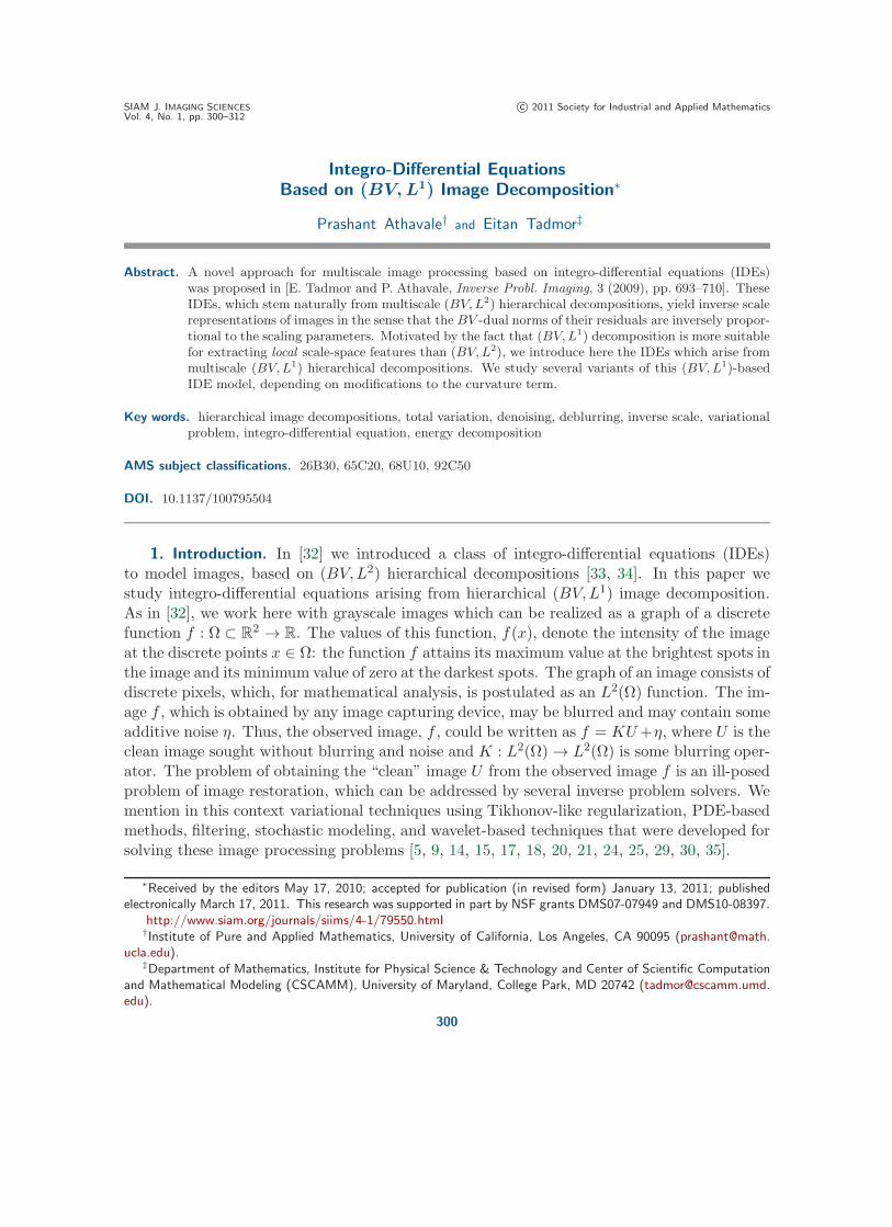
SIAM J. IMAGING SCIENCES c© 2011 Society for Industrial and Applied MathematicsVol. 4, No. 1, pp. 300–312

Integro-Differential EquationsBased on (BV,L1) Image Decomposition∗

Prashant Athavale† and Eitan Tadmor‡

Abstract. A novel approach for multiscale image processing based on integro-differential equations (IDEs)was proposed in [E. Tadmor and P. Athavale, Inverse Probl. Imaging, 3 (2009), pp. 693–710]. TheseIDEs, which stem naturally from multiscale (BV,L2) hierarchical decompositions, yield inverse scalerepresentations of images in the sense that the BV -dual norms of their residuals are inversely propor-tional to the scaling parameters. Motivated by the fact that (BV,L1) decomposition is more suitablefor extracting local scale-space features than (BV,L2), we introduce here the IDEs which arise frommultiscale (BV,L1) hierarchical decompositions. We study several variants of this (BV,L1)-basedIDE model, depending on modifications to the curvature term.

Key words. hierarchical image decompositions, total variation, denoising, deblurring, inverse scale, variationalproblem, integro-differential equation, energy decomposition

AMS subject classifications. 26B30, 65C20, 68U10, 92C50

DOI. 10.1137/100795504

1. Introduction. In [32] we introduced a class of integro-differential equations (IDEs)to model images, based on (BV,L2) hierarchical decompositions [33, 34]. In this paper westudy integro-differential equations arising from hierarchical (BV,L1) image decomposition.As in [32], we work here with grayscale images which can be realized as a graph of a discretefunction f : Ω ⊂ R2 → R. The values of this function, f(x), denote the intensity of the imageat the discrete points x ∈ Ω: the function f attains its maximum value at the brightest spots inthe image and its minimum value of zero at the darkest spots. The graph of an image consists ofdiscrete pixels, which, for mathematical analysis, is postulated as an L2(Ω) function. The im-age f , which is obtained by any image capturing device, may be blurred and may contain someadditive noise η. Thus, the observed image, f , could be written as f = KU+η, where U is theclean image sought without blurring and noise and K : L2(Ω) → L2(Ω) is some blurring oper-ator. The problem of obtaining the “clean” image U from the observed image f is an ill-posedproblem of image restoration, which can be addressed by several inverse problem solvers. Wemention in this context variational techniques using Tikhonov-like regularization, PDE-basedmethods, filtering, stochastic modeling, and wavelet-based techniques that were developed forsolving these image processing problems [5, 9, 14, 15, 17, 18, 20, 21, 24, 25, 29, 30, 35].

∗Received by the editors May 17, 2010; accepted for publication (in revised form) January 13, 2011; publishedelectronically March 17, 2011. This research was supported in part by NSF grants DMS07-07949 and DMS10-08397.

http://www.siam.org/journals/siims/4-1/79550.html†Institute of Pure and Applied Mathematics, University of California, Los Angeles, CA 90095 (prashant@math.

ucla.edu).‡Department of Mathematics, Institute for Physical Science & Technology and Center of Scientific Computation

and Mathematical Modeling (CSCAMM), University of Maryland, College Park, MD 20742 ([email protected]).

300

http://www.siam.org/journals/siims/4-1/79550.html

mailto:[email protected]




(BV,L1) INTEGRO-DIFFERENTIAL EQUATIONS FOR IMAGES 301

Image restoration leads to image decomposition. For example, any denoising of an observedimage f results in the decomposing of type f = Uλ + ηλ, where ηλ is interpreted as a noiseby the denoising method. Here, λ is an algorithm-specific scaling parameter : in the case ofGaussian smoothing, for example, the variance of the Gaussian kernel may serve as such ascaling parameter. Small-scale features, categorized as noise, are then forced into ηλ, resultingin a larger-scale version, Uλ, of the original image f .

1.1. PDE-based, variational, and hierarchical decompositions. Two main approachesfor multiscale representations of images are PDE-based methods and variational methods.The basic PDE-based method is the heat equation, ut = Δu, where, starting with the givenimage as initial condition, u(0) := f , it produces a multiscale representation, {u(t)}t>0, for theimage f . The heat equation removes noise through blurring, but being an isotropic diffusionit also blurs edges which define main features in the image. This drawback can be removedby using instead the Perona–Malik [29] nonlinear equation based on nonisotropic diffusion,ut = div(g(|∇u|)∇u). The equation is ill-posed, however, and as already noted by theseauthors, the Perona–Malik diffusion can lead to false detection of edges in the presence ofnoise. To resolve this issue, Catte et al. [11] proposed using a modified nonisotropic andnonlocal diffusive amplitude of the form g(|Gσ � ∇u|); this class of methods was studied in[19, 36]. All these methods give rise to a forward multiscale representation of the image f , inthe sense that u(t) begins with the finest scale, u(0) := f , and then progressively blurs intocoarser representations of f as t → ∞.

The class of variational methods is a widely used alternative to PDE-based methods inimage processing. Methods such as Mumford–Shah segmentation [25, 26] and Rudin–Osher–Fatemi (ROF) decomposition [30] fall under a general category of Tikhonov regularization[35, 31]. Here one attempts to find a close approximation to a function f ∈ Y , in a spaceX � Y , which is an appropriate space adapted to measure edges and textures sought in u.This leads to the following minimization problem:

f = uλ + vλ, [uλ, vλ] := arginff=u+v

{ ‖u‖X + λ ‖v‖Y}.

The term ‖u‖X is a regularizing term, and uλ + vλ is a multiscale decomposition of f whichvaries with the positive scaling parameter, λ. For references on this class of “u+ v” methodswe refer the reader to [10]. In the case of the ROF model [30], for example, edges are soughtin the space of bounded variations, X = BV (Ω) and f ∈ Y = L2; see, e.g., [6]. This yieldsthe (BV,L2)-decomposition:

(1.1) f = uλ + vλ, [uλ, vλ] := arginff=u+v

{ |u|BV + λ ‖v‖2L2

},

where |u|BV :=∫Ω |∇u| is the BV -seminorm. For small values of λ, the minimizer uλ is

a large-scale image which consists of only main features and prominent edges in f . As λbecomes larger, uλ captures the small-scale details of f . The point of view advocated in [33]is to replace the fixed scaling parameter λ by a varying sequence of inverse-scale parameters,λ1 < λ2 < · · · , which dictate the scaling of the iterative refinement step,

[uλj+1, vλj+1

] := arginfvλj=u+v

{ |u|BV + λj+1 ‖v‖2L2

},(1.2a)

302 PRASHANT ATHAVALE AND EITAN TADMOR

which in turn generates a multiscale (BV,L2) hierarchical representation,

f ≈∑j

uλj.(1.2b)

2. A novel (BV,L1)-based integro-differential equation (IDE). In [32] we introducedthe integro-differential equation1

(2.1)

∫ t

0u(x, s) ds = f(x) +

1

2λ(t)div

( ∇u(x, t)

|∇u(x, t)|),

∂u

∂n

∣∣∣∂Ω

= 0.

This novel IDE was based on a hierarchical (BV,L2) decomposition (1.2) which was introducedby Tadmor, Nezzar, and Vese [33, 34], from which it inherits many important properties. Oncewe were dealing with the framework of IDEs, several extensions of (2.1) were proposed in [32]to deal with denoising and deblurring of images, which were not strictly associated with anyvariational problem.

The ROF decomposition (1.1) uses the L2-fidelity term ‖f − u‖2L2 . An alternative varia-tional problem based on an L1-fidelity term, ‖f − u‖L1 , was proposed earlier by Alliney [4]and was studied extensively by Chan, Esedoglu, and Nikolova (see [12, 27, 13]):

(2.2) f = uλ + vλ, [uλ, vλ] := arginff=u+v

{ |u|BV + λ ‖v‖L1

}.

The resulting (BV,L1) minimization1 differs from the (BV,L2) model in several importantaspects which have attracted considerable attention in recent years; see [1, 2, 3, 16]. We shallmention two such aspects. The (BV,L1) minimization is contrast invariant, as opposed tothe (BV,L2) minimization. Chan and Esedoglu [12] also showed the more local geometricaspects of the (BV,L1) minimization. In particular, recall that if supp(f) ∈ BR(0), then boththe (BV,L1) and the (BV,L2) minimizers vanish, namely, uλ ≡ 0 and vλ = f for small λ’sbelow the minimal threshold λ < λL ∝ 1

R . On the other hand, if the f is a characteristicfunction χΣ, then the (BV,L1) minimizer of (2.2) admits a maximal threshold, λH , such thatfor all λ > λH we have uλ = f and vλ ≡ 0, in contrast to the “leaking” phenomenon with the(BV,L2)-based ROF model, where vλ ∝ 1

R [22].

2.1. Quantization. To proceed with the derivation of a (BV,L1)-based IDE, we first needto address a proper quantization of the image intensity. If we let τ denote the small intensityquanta, then we can rescale the coarse image in (2.2), uλ, in τ -units. With this in mind, wedecompose the given image f using the (BV,L1) scheme, starting with initial scale λ0:

f = uλ0τ + vλ0 , uλ0 := arginfu

{|u|BV +

λ0

τ‖f − uτ‖L1

}.

1The term div( ∇u(·,t)|∇u(·,t)|

), which often arises in image processing, is the curvature of isolevel curves of

function u(·, t) [8, 7]. In the present context, it arises as the first variation of the BV -norm, |u|BV , which in

practice is replaced by its regularized form, e.g., |u|BV =√

|∇u|2L1 + ε2, thus removing the ambiguity when∇u = 0 and the possible lack of uniqueness in the corresponding (BV,L1) minimization in (2.2) [1, 3].


The residual image vλ0 := f − uλ0τ can be further decomposed into a smaller scale withλ1 > λ0:

vλ0 = uλ1τ + vλ1 , uλ1 := arginfu

{|u|BV +

λ1

τ‖vλ0 − uτ‖L1

}.

We can continue this process for λ0 < λ1 < λ2 < · · · :

vλk−1= uλk

τ + vλk, uλk

:= arginfu

{|u|BV +

λk

τ‖vλk−1

− uτ‖L1

}.

A telescoping sum of the refinement step vλk−1− vλk

= uλkτ yields the following hierarchical

(BV,L1) decomposition of f :

f = uλ0τ + vλ0

= uλ0τ + uλ1τ + vλ1

= · · ·= uλ0τ + uλ1τ + · · · + uλN

τ + vλN.

Remark 2.1. We note that in order to begin with only the main features of f , the initialscale needs to be small but not too small: to capture a nontrivial minimizer, λ0 needs to belarger than a minimal threshold, which is quantified in terms of the dual ‖ · ‖∗-norm specifiedin (2.7) below [34, eq. (2.5)], [22]; i.e.,

(2.3) λ0 > λL := 1/‖sgn(f)‖∗.

This yields a hierarchical (BV,L1) multiscale image decomposition,

(2.4) f =N∑

k=k0

uλkτ + vλN

,

where k0 signals the initial scale λk0 to yield the first nontrivial minimizer uλ0 . Consider theNth step in the (BV,L1) scheme,

uλN= arginf

u

(∫Ω|∇u|+ λN

τ

∫Ω|vλN−1

− uτ |).

The Euler–Lagrange equation associated with this minimizer reads (with the usual under-standing of a regularized curvature term) as

(2.5) sgn (uλNτ − vλN−1

) =1

λNdiv

( ∇uλN

|∇uλN|).

From (2.4) we have

vλN−1= f −

N−1∑k=k0

uλkτ,


and using this above expression in (2.5) we find

sgn

⎛⎝ N∑

k=k0

uλkτ − f

⎞⎠ =

1

λNdiv

( ∇uλN

|∇uλN|).

Letting τ → 0, we arrive at the following (BV,L1) IDE:

(2.6) sgn

(∫ t

s=t0

u(x, s) ds − f(x)

)=

1

λ(t)div

( ∇u(x, t)

|∇u(x, t)|),

∂u

∂n

∣∣∣∂Ω

= 0, t ≥ t0,

subject to the initial condition u(·, t0) = 0. The scaling function λ(t) is any monotoneincreasing function at our disposal. We discuss the role of this function in the next section.

2.2. On the scaling function λ(t). It is argued in [22] that the dual norm,

(2.7) ‖w‖∗ := sup|ϕ|BV �=0

〈w,ϕ − ϕ〉L2

|ϕ|BV, ϕ =

1

|Ω|∫Ωϕ(x)dx,

is a proper norm to measure texture (equivalently, one can characterize this dual norm as‖w‖∗ := infg{‖g‖L∞ : div g = w−w}). To understand the critical role of the scaling functionλ(t) in the IDE model (2.6) and its relationship with the “star-norm,” we first prove thefollowing useful lemma.

Lemma 2.1. For u ∈ BV , let κu be the curvature term, κu := div( ∇u|∇u|

), whenever |∇u| �=

0. Then‖κu‖∗ = 1.

Proof. For ϕ ∈ BV we have the following:

(2.8) |(κu, ϕ)L2 | =∣∣∣∣(div

( ∇u

|∇u|), ϕ

)L2

∣∣∣∣ ≤ |ϕ|BV .

Thus, we have ‖κu‖∗ ≤ 1. Letting ϕ = u in (2.8), we obtain |〈κu, u〉L2 | = |u|BV and the resultfollows.

The following theorem is a direct consequence of this lemma.Theorem 2.2. Consider the IDE model (2.6)

sgn (U(x, t)− f(x)) =1

λ(t)div

( ∇u(x, t)

|∇u(x, t)|), U(x, t) :=

∫ t

t0

u(x, s) ds.

Then, the size of the residual, V (·, t) := f − ∫ tt0u(·, s) ds, is dictated by the scaling function

λ(t): ∥∥sgn(V (·, t))∥∥∗ = 1

λ(t).

The “star-norm” measures oscillations [22]. Thus, the above equality could be interpretedas saying that the oscillations in the residual image V (·, t) are inversely proportional to thescaling function λ(t). In particular, the oscillations in the residual function diminish in aprecise manner controlled by increasing λ(t).


Remark 2.2. Recall that t0 in Theorem 2.2 is determined as the minimal effective scalein the sense that (2.3) holds; i.e., λ(t0) > λL = 1/‖sgn(f)‖∗. One does not need, however,to have a priori knowledge on the amount of “star-norm” oscillation in f , since U(·, t) ≡ 0 aslong as λ(t) is underestimated, i.e., λ < λL. Eventually, the increasing λ(t) will pick up theminimal effective scale.

2.3. L1-energy decomposition. The increase of λ(t) is directly linked to the “energy”of the underlying image. For the (BV,L2)-based IDE (2.1), we proved in [32] the L2-energydecomposition ∫ t

s=t0

1

λ(s)|u(·, s)|BV ds+ ‖V (·, t)‖2L2 = ‖f‖2L2 .

For the (BV,L1)-based IDE we have the corresponding L1-energy decomposition.

Proposition 2.3. Consider the IDE (2.6) and let V (·, t) denote the residual, V (·, t) :=∫ tt0u(·, s) ds − f . Then we have the following L1-energy decomposition:

∫ t

t0

1

λ(s)|u(·, s)|BV ds+ ‖V (·, t)‖L1 = ‖f‖L1 .

Proof. We denote by U(·, t) :=∫ tt0u(·, s) ds the cumulative image so that the IDE (2.6)

takes the form1

λ(t)div

( ∇u(x, t)

|∇u(x, t)|)

= sgn(U(x, t) − f(x)).

Integrating the above against u ≡ ddt(U − f), we get

− 1

λ(t)|u(·, t)|BV =

∫Ωsgn(U(·, t) − f)

d

dt

(U(·, t)− f

)dx

=d

dt

∫Ωsgn(U(·, t) − f) (U(·, t)− f) dx =

d

dt

∫Ω|U(·, t) − f | dx,

and the result follows by time integration.

3. IDEs for images: Numerical results and extensions.

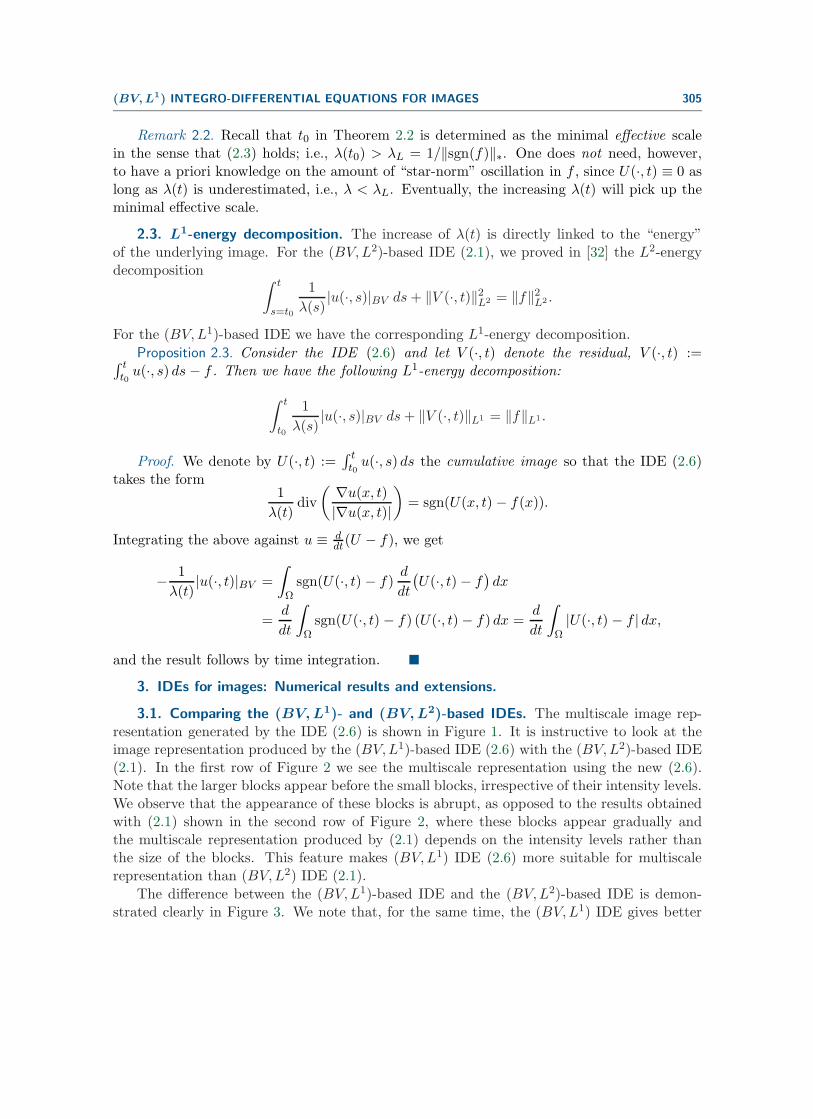
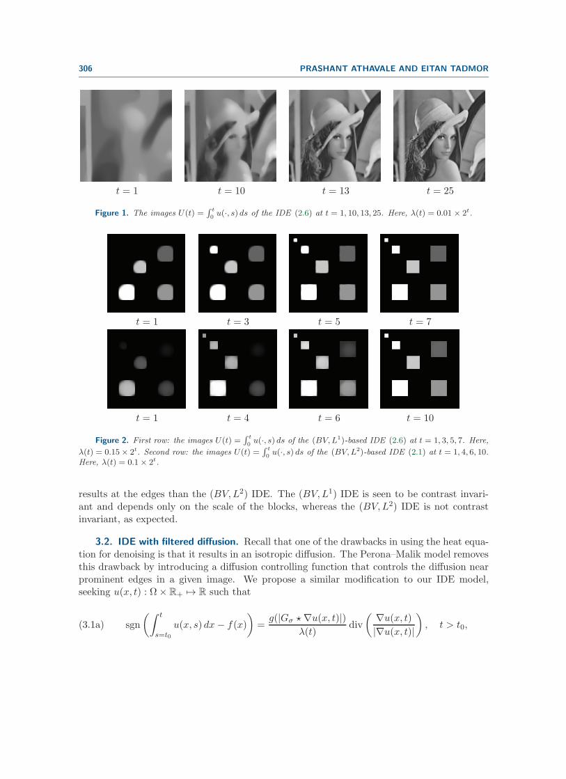
3.1. Comparing the (BV,L1)- and (BV,L2)-based IDEs. The multiscale image rep-resentation generated by the IDE (2.6) is shown in Figure 1. It is instructive to look at theimage representation produced by the (BV,L1)-based IDE (2.6) with the (BV,L2)-based IDE(2.1). In the first row of Figure 2 we see the multiscale representation using the new (2.6).Note that the larger blocks appear before the small blocks, irrespective of their intensity levels.We observe that the appearance of these blocks is abrupt, as opposed to the results obtainedwith (2.1) shown in the second row of Figure 2, where these blocks appear gradually andthe multiscale representation produced by (2.1) depends on the intensity levels rather thanthe size of the blocks. This feature makes (BV,L1) IDE (2.6) more suitable for multiscalerepresentation than (BV,L2) IDE (2.1).

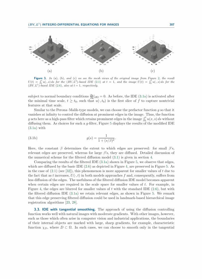
The difference between the (BV,L1)-based IDE and the (BV,L2)-based IDE is demon-strated clearly in Figure 3. We note that, for the same time, the (BV,L1) IDE gives better


t = 1 t = 10 t = 13 t = 25

Figure 1. The images U(t) =∫ t

0u(·, s) ds of the IDE (2.6) at t = 1, 10, 13, 25. Here, λ(t) = 0.01 × 2t.

t = 1 t = 3 t = 5 t = 7

t = 1 t = 4 t = 6 t = 10

Figure 2. First row: the images U(t) =∫ t

0u(·, s) ds of the (BV,L1)-based IDE (2.6) at t = 1, 3, 5, 7. Here,

λ(t) = 0.15× 2t. Second row: the images U(t) =∫ t

0u(·, s) ds of the (BV,L2)-based IDE (2.1) at t = 1, 4, 6, 10.

Here, λ(t) = 0.1× 2t.

results at the edges than the (BV,L2) IDE. The (BV,L1) IDE is seen to be contrast invari-ant and depends only on the scale of the blocks, whereas the (BV,L2) IDE is not contrastinvariant, as expected.

3.2. IDE with filtered diffusion. Recall that one of the drawbacks in using the heat equa-tion for denoising is that it results in an isotropic diffusion. The Perona–Malik model removesthis drawback by introducing a diffusion controlling function that controls the diffusion nearprominent edges in a given image. We propose a similar modification to our IDE model,seeking u(x, t) : Ω× R+ �→ R such that

sgn

(∫ t

s=t0

u(x, s) dx− f(x)

)=

g(|Gσ �∇u(x, t)|)λ(t)

div

( ∇u(x, t)

|∇u(x, t)|), t > t0,(3.1a)


(a) (b) (c)

Figure 3. In (a), (b), and (c) we see the mesh views of the original image from Figure 2, the resultU(t) =

∫ t

0u(·, s) ds for the (BV,L2)-based IDE (2.1) at t = 1, and the image U(t) =

∫ t

0u(·, s) ds for the

(BV,L1)-based IDE (2.6), also at t = 1, respectively.

subject to normal boundary conditions ∂u∂n |∂Ω = 0. As before, the IDE (3.1a) is activated after

the minimal time scale, t ≥ t0, such that u(·, t0) is the first slice of f to capture nontrivialfeatures at that scale.

Similar to the Perona–Malik-type models, we can choose the prefactor function g so that itvanishes at infinity to control the diffusion at prominent edges in the image. Thus, the functiong acts here as a high-pass filter which retains prominent edges in the image

∫ t0 u(x, s) ds without

diffusing them. As choices for such a g-filter, Figure 5 displays the results of the modified IDE(3.1a) with

g(s) =1

1 + (s/β)2.(3.1b)

Here, the constant β determines the extent to which edges are preserved: for small β’s,relevant edges are preserved, whereas for large β’s, they are diffused. Detailed discussion ofthe numerical scheme for the filtered diffusion model (3.1) is given in section 4.

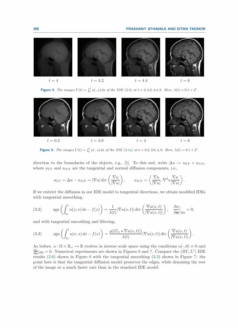
Comparing the results of the filtered IDE (3.1a) shown in Figure 5, we observe that edges,which are diffused by the basic IDE (2.6) as depicted in Figure 4, are preserved in Figure 5. Asin the case of (2.1) (see [32]), this phenomenon is more apparent for smaller values of t due tothe fact that as t increases, U(·, t) in both models approaches f and, consequently, suffers fromless diffusion of the edges. The usefulness of the filtered diffusion IDE model becomes apparentwhen certain edges are required in the scale space for smaller values of t. For example, inFigure 4, the edges are blurred for smaller values of t with the standard IDE (2.6), but withthe filtered diffusion IDE (3.1a) we retain relevant edges, as shown in Figure 5. We remarkthat this edge preserving filtered diffusion could be used in landmark-based hierarchical imageregistration algorithms [23, 28].

3.3. IDE with tangential smoothing. The approach of using the diffusion controllingfunction works well with natural images with moderate gradients. With other images, however,such as those which often arise in computer vision and industrial applications, the boundariesof their internal objects are marked with large, sharp gradients, for example, characteristicfunction χD, where D ⊂ Ω. In such cases, we can choose to smooth only in the tangential


t = 4 t = 4.2 t = 4.4 t = 6


0u(·, s) ds of the IDE (2.6) at t = 4, 4.2, 4.4, 6. Here, λ(t) = 0.1 × 2t.

t = 0.2 t = 3.8 t = 4 t = 6


0u(·, s) ds of the IDE (3.1a) at t = 0.2, 3.8, 4, 6. Here, λ(t) = 0.1× 2t.

direction to the boundaries of the objects, e.g., [5]. To this end, write Δu := uTT + uNN ,where uTT and uNN are the tangential and normal diffusion components, i.e.,

uTT = Δu− uNN = |∇u|div( ∇u

|∇u|), uNN =

⟨ ∇u

|∇u| ,∇2u

∇u

|∇u|⟩.

If we restrict the diffusion in our IDE model to tangential directions, we obtain modified IDEswith tangential smoothing,

(3.2) sgn

(∫ t

t0

u(x, s) ds − f(x)

)=

1

λ(t)|∇u(x, t)|div

( ∇u(x, t)

|∇u(x, t)|),

∂u

∂n

∣∣∣∂Ω

= 0,

and with tangential smoothing and filtering,

(3.3) sgn

(∫ t

t0

u(x, s) ds − f(x)

)=

g(|Gσ �∇u(x, t)|)λ(t)

|∇u(x, t)|div( ∇u(x, t)

|∇u(x, t)|).

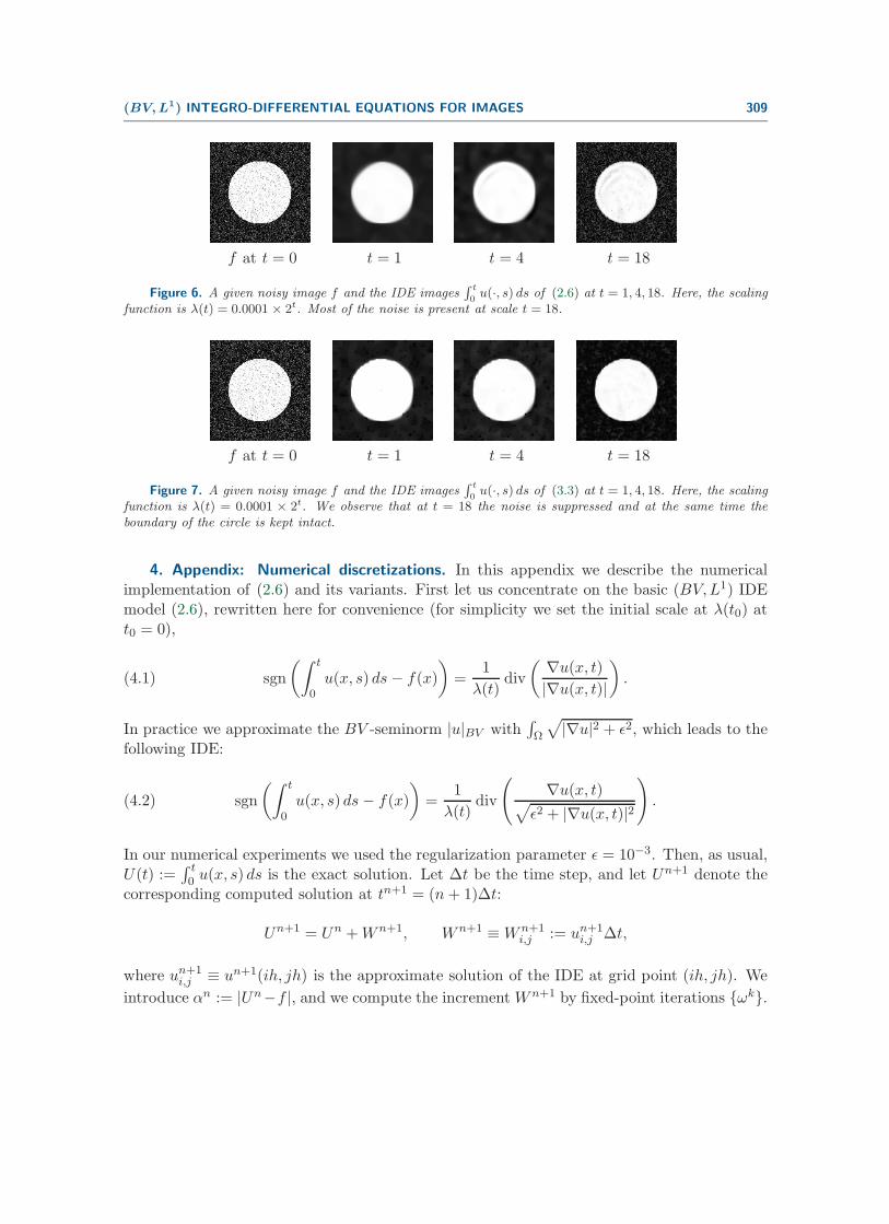
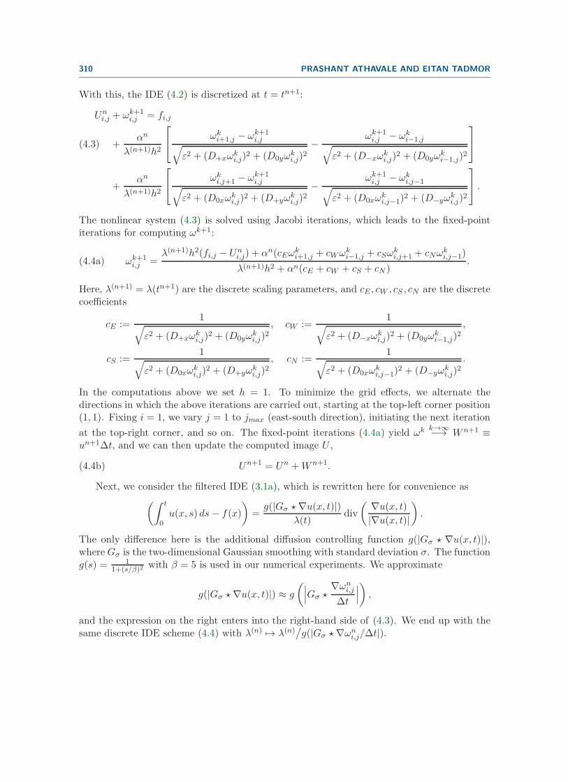
As before, u : Ω× R+ �→ R evolves in inverse scale space using the conditions u(·, 0) ≡ 0 and∂u∂n |∂Ω = 0. Numerical experiments are shown in Figures 6 and 7. Compare the (BV,L1) IDEresults (2.6) shown in Figure 6 with the tangential smoothing (3.3) shown in Figure 7: thepoint here is that the tangential diffusion model preserves the edges, while denoising the restof the image at a much faster rate than in the standard IDE model.


f at t = 0 t = 1 t = 4 t = 18

Figure 6. A given noisy image f and the IDE images∫ t

0u(·, s) ds of (2.6) at t = 1, 4, 18. Here, the scaling

function is λ(t) = 0.0001 × 2t. Most of the noise is present at scale t = 18.

f at t = 0 t = 1 t = 4 t = 18

Figure 7. A given noisy image f and the IDE images∫ t

0u(·, s) ds of (3.3) at t = 1, 4, 18. Here, the scaling

function is λ(t) = 0.0001 × 2t. We observe that at t = 18 the noise is suppressed and at the same time theboundary of the circle is kept intact.

4. Appendix: Numerical discretizations. In this appendix we describe the numericalimplementation of (2.6) and its variants. First let us concentrate on the basic (BV,L1) IDEmodel (2.6), rewritten here for convenience (for simplicity we set the initial scale at λ(t0) att0 = 0),

(4.1) sgn

(∫ t

0u(x, s) ds − f(x)

)=

1

λ(t)div

( ∇u(x, t)

|∇u(x, t)|).

In practice we approximate the BV -seminorm |u|BV with∫Ω

√|∇u|2 + ε2, which leads to the

following IDE:

(4.2) sgn

(∫ t

0u(x, s) ds − f(x)

)=

1

λ(t)div

(∇u(x, t)√

ε2 + |∇u(x, t)|2

).

In our numerical experiments we used the regularization parameter ε = 10−3. Then, as usual,U(t) :=

∫ t0 u(x, s) ds is the exact solution. Let Δt be the time step, and let Un+1 denote the

corresponding computed solution at tn+1 = (n+ 1)Δt:

Un+1 = Un +W n+1, W n+1 ≡ W n+1i,j := un+1

i,j Δt,

where un+1i,j ≡ un+1(ih, jh) is the approximate solution of the IDE at grid point (ih, jh). We

introduce αn := |Un−f |, and we compute the increment W n+1 by fixed-point iterations {ωk}.


With this, the IDE (4.2) is discretized at t = tn+1:

Uni,j + ωk+1

i,j = fi,j

+αn

λ(n+1)h2

⎡⎣ ωk

i+1,j − ωk+1i,j√

ε2 + (D+xωki,j)

2 + (D0yωki,j)

2− ωk+1

i,j − ωki−1,j√

ε2 + (D−xωki,j)

2 + (D0yωki−1,j)

2

⎤⎦(4.3)

+αn

λ(n+1)h2

⎡⎣ ωk

i,j+1 − ωk+1i,j√

ε2 + (D0xωki,j)

2 + (D+yωki,j)

2− ωk+1

i,j − ωki,j−1√

ε2 + (D0xωki,j−1)

2 + (D−yωki,j)

2

⎤⎦ .

The nonlinear system (4.3) is solved using Jacobi iterations, which leads to the fixed-pointiterations for computing ωk+1:

ωk+1i,j =

λ(n+1)h2(fi,j − Uni,j) + αn(cEω

ki+1,j + cWωk

i−1,j + cSωki,j+1 + cNωk

i,j−1)

λ(n+1)h2 + αn(cE + cW + cS + cN ).(4.4a)

Here, λ(n+1) = λ(tn+1) are the discrete scaling parameters, and cE , cW , cS , cN are the discretecoefficients

cE :=1√

ε2 + (D+xωki,j)

2 + (D0yωki,j)

2, cW :=

1√ε2 + (D−xω

ki,j)

2 + (D0yωki−1,j)

2,

cS :=1√

ε2 + (D0xωki,j)

2 + (D+yωki,j)

2, cN :=

1√ε2 + (D0xω

ki,j−1)

2 + (D−yωki,j)

2.

In the computations above we set h = 1. To minimize the grid effects, we alternate thedirections in which the above iterations are carried out, starting at the top-left corner position(1, 1). Fixing i = 1, we vary j = 1 to jmax (east-south direction), initiating the next iteration

at the top-right corner, and so on. The fixed-point iterations (4.4a) yield ωk k→∞−→ W n+1 ≡un+1Δt, and we can then update the computed image U ,

Un+1 = Un +W n+1.(4.4b)

Next, we consider the filtered IDE (3.1a), which is rewritten here for convenience as(∫ t

0u(x, s) ds − f(x)

)=

g(|Gσ �∇u(x, t)|)λ(t)

div

( ∇u(x, t)

|∇u(x, t)|).

The only difference here is the additional diffusion controlling function g(|Gσ � ∇u(x, t)|),whereGσ is the two-dimensional Gaussian smoothing with standard deviation σ. The functiong(s) = 1

1+(s/β)2with β = 5 is used in our numerical experiments. We approximate

g(|Gσ �∇u(x, t)|) ≈ g

(∣∣∣Gσ �∇ωn

i,j

Δt

∣∣∣) ,

and the expression on the right enters into the right-hand side of (4.3). We end up with thesame discrete IDE scheme (4.4) with λ(n) �→ λ(n)

/g(|Gσ �∇ωn

i,j/Δt|).


REFERENCES

[1] W. K. Allard, Total variation regularization for image denoising, I. Geometric theory, SIAM J. Math.Anal., 39 (2007), pp. 1150–1190.

[2] W. K. Allard, Total variation regularization for image denoising, II. Examples, SIAM J. Imaging Sci.,1 (2008), pp. 400–417.

[3] W. K. Allard, Total variation regularization for image denoising, III. Examples, SIAM J. Imaging Sci.,2 (2009), pp. 532–568.

[4] S. Alliney, Digital filters as absolute norm regularizers, IEEE Trans. Signal Process., 40 (1992), pp.1548–1562.

[5] L. Alvarez, P.-L. Lions, and J.-M. Morel, Image selective smoothing and edge detection by nonlineardiffusion. II, SIAM J. Numer. Anal., 29 (1992), pp. 845–866.

[6] L. Ambrosio, N. Fusco, and D. Pallara, Functions of Bounded Variation and Free DiscontinuityProblems, Oxford Math. Monogr., The Clarendon Press, Oxford University Press, New York, 2000.

[7] F. Andreu-Vaillo, V. Casalles, and J. Mazon, Parabolic Quasilinear Equations Minimizing LinearGrowth Functionals, Progr. Math. 223, Birkhauser, Basel, Switzerland, 2004.

[8] G. Aubert and P. Kornprobst, Mathematical Problems in Image Processing. Partial Differential Equa-tions and the Calculus of Variations, 2nd ed., Appl. Math. Sci. 147, Springer-Verlag, New York, 2006.

[9] G. Aubert and L. Vese, A variational method in image recovery, SIAM J. Numer. Anal., 34 (1997),pp. 1948–1979.

[10] A. Buades, T. Le, J.-M. Morel, and L. Vese, Fast cartoon + texture image filters, IEEE Trans.Image Process., 19 (2010), pp. 1978–1986.

[11] F. Catte, P.-L. Lions, J.-M. Morel, and T. Coll, Image selective smoothing and edge detection bynonlinear diffusion, SIAM J. Numer. Anal., 29 (1992), pp. 182–193.

[12] T. F. Chan and S. Esedoglu, Aspects of total variation regularized L1 function approximation, SIAMJ. Appl. Math., 65 (2005), pp. 1817–1837.

[13] T. F. Chan, S. Esedoglu, and M. Nikolova, Algorithms for finding global minimizers of imagesegmentation and denoising models, SIAM J. Appl. Math., 66 (2006), pp. 1632–1648.

[14] T. F. Chan and J. Shen, Image Processing and Analysis: Variational, PDE, Wavelet, and StochasticMethods, SIAM, Philadelphia, 2005.

[15] T. F. Chan, J. Shen, and L. Vese, Variational PDE models in image processing, Notices Amer. Math.Soc., 50 (2003), pp. 14–26.

[16] V. Duval, J.-F. Aujol, and Y. Gousseau, The TVL1 model: A geometric point of view, MultiscaleModel. Simul., 8 (2009), pp. 154–189.

[17] S. Esedoglu and S. J. Osher, Decomposition of images by the anisotropic Rudin-Osher-Fatemi model,Comm. Pure Appl. Math., 57 (2004), pp. 1609–1626.

[18] S. Geman and D. Geman, Stochastic relaxation, Gibbs distributions, and the Bayesian restoration ofimages, IEEE Trans. Pattern Anal. Mach. Intell., 6 (1984), pp. 721–741.

[19] P. Guidotti, A new well-posed nonlinear nonlocal diffusion, Nonlinear Anal., 72 (2010), pp. 4625–4637.[20] S. Li, Markov Random Field Modeling in Computer Vision, Springer-Verlag, London, 1995.[21] S. Mallat, A Wavelet Tour of Signal Processing, Academic Press, San Diego, CA, 1998.[22] Y. Meyer, Oscillating Patterns in Image Processing and Nonlinear Evolution Equations. The Fifteenth

Dean Jacqueline B. Lewis Memorial Lectures, Univ. Lecture Ser. 22, American Mathematical Society,Providence, RI, 2001.

[23] J. Modersitzki, Numerical Methods for Image Registration, Oxford University Press, New York, 2004.[24] V. Morozov, Regularization Methods for Ill-Posed Problems, CRC Press, Boca Raton, FL, 1993. Trans-

lated from the 1987 Russian original.[25] D. Mumford and J. Shah, Boundary detection by minimizing functionals, in Proceedings of the IEEE

Computer Society Conference on Computer Vision and Pattern Recognition, San Francisco, CA, 1985,pp. 22–26.

[26] D. Mumford and J. Shah, Optimal approximations by piecewise smooth functions and associated vari-ational problems, Comm. Pure Appl. Math., 42 (1989), pp. 577–685.

[27] M. Nikolova, Minimizers of cost-functions involving nonsmooth data-fidelity terms. Application to theprocessing of outliers, SIAM J. Numer. Anal., 40 (2002), pp. 965–994.


[28] D. Paquin, D. Levy, E. Schreibmann, and L. Xing, Multiscale image registration, Math. Biosci. Eng.,3 (2006), pp. 389–418.

[29] P. Perona and J. Malik, Scale-space and edge detection using anisotropic diffusion, IEEE Trans.Pattern Anal. Mach. Intell., 12 (1990), pp. 629–639.

[30] L. Rudin, S. Osher, and E. Fatemi, Nonlinear total variation based noise removal algorithms, Phys.D, 60 (1992), pp. 259–268.

[31] O. Scherzer, M. Grasmair, H. Grossauer, M. Haltmeier, and F. Lenzen, Variational Methods inImaging, Appl. Math. Sci. 167, Springer-Verlag, New York, 2009.

[32] E. Tadmor and P. Athavale, Multiscale image representation using novel integro-differential equations,Inverse Probl. Imaging, 3 (2009), pp. 693–710.

[33] E. Tadmor, S. Nezzar, and L. Vese, A multiscale image representation using hierarchical (BV,L2)decompositions, Multiscale Model. Simul., 2 (2004), pp. 554–579.

[34] E. Tadmor, S. Nezzar, and L. Vese, Multiscale hierarchical decomposition of images with applicationsto deblurring, denoising and segmentation, Commun. Math. Sci., 6 (2008), pp. 1–26.

[35] A. Tikhonov and V. Arsenin, Solutions of Ill-Posed Problems, Scripta Series in Mathematics, V. H.Winston & Sons, Washington, D.C., John Wiley & Sons, New York, 1977. Translated from theRussian.

[36] J. Weickert, Anisotropic Diffusion in Image Processing, Teubner-Verlag, Stuttgart, Germany, 1998.

Integro-Diﬀerential Equations Basedon BV,L …€¦ · Integro-Diﬀerential Equations...

Documents

Transcript of Integro-Diﬀerential Equations Basedon BV,L …€¦ · Integro-Diﬀerential Equations...