Integral Transforms

1

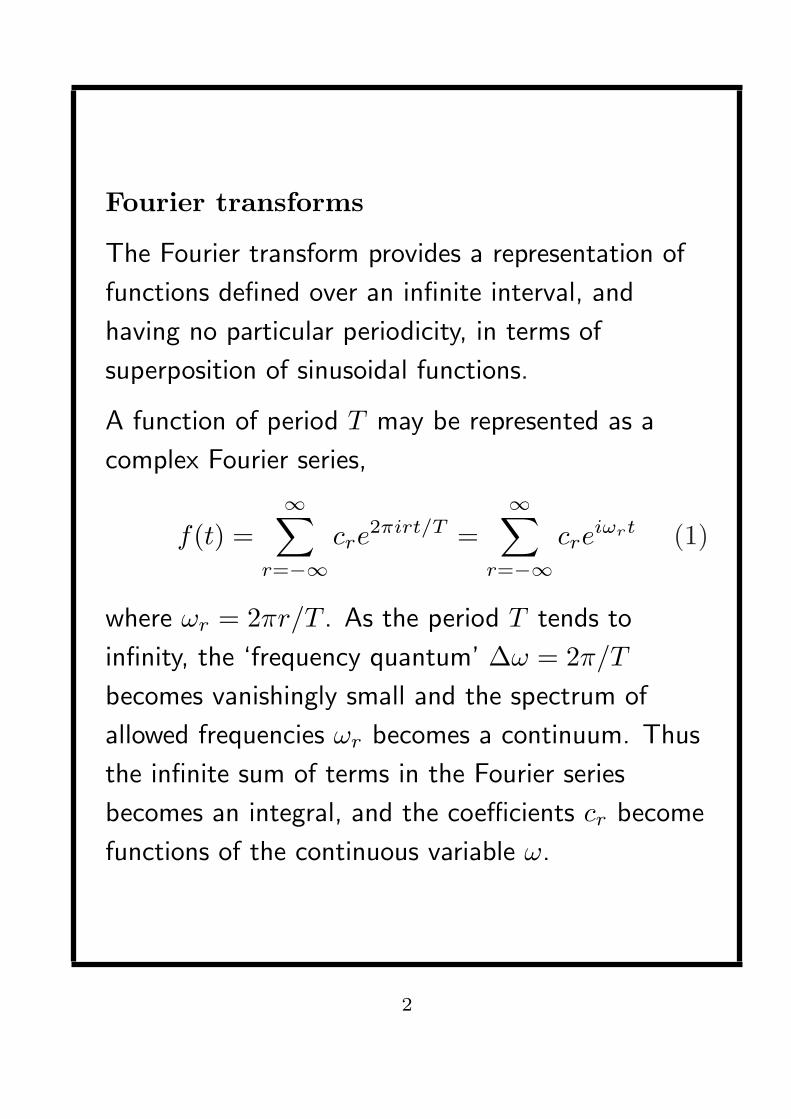
Fourier transforms

The Fourier transform provides a representation of

functions defined over an infinite interval, and

having no particular periodicity, in terms of

superposition of sinusoidal functions.

A function of period T may be represented as a

complex Fourier series,

f(t) =∞∑

r=−∞cre

2πirt/T =∞∑

r=−∞cre

iωrt (1)

where ωr = 2πr/T . As the period T tends to

infinity, the ‘frequency quantum’ ∆ω = 2π/T

becomes vanishingly small and the spectrum of

allowed frequencies ωr becomes a continuum. Thus

the infinite sum of terms in the Fourier series

becomes an integral, and the coefficients cr become

functions of the continuous variable ω.

2

We recall that the coefficients cr in Eq. (1) are

given by

cr =1T

∫ T/2

−T/2

f(t)e−2πirt/T dt

=∆ω

2π

∫ T/2

−T/2

f(t)e−iωrt dt. (2)

Substituting from Eq. (2) and into (1) gives

f(t) =∞∑

r=−∞

∆ω

2π

∫ T/2

−T/2

f(u)e−iωru dueiωrt. (3)

At this stage, ωr is still a discrete function of r

equal to 2πr/T .

3

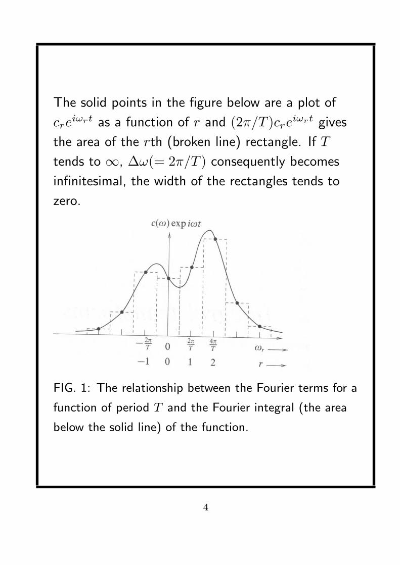
The solid points in the figure below are a plot of

creiωrt as a function of r and (2π/T )cre

iωrt gives

the area of the rth (broken line) rectangle. If T

tends to ∞, ∆ω(= 2π/T ) consequently becomes

infinitesimal, the width of the rectangles tends to

zero.

FIG. 1: The relationship between the Fourier terms for a

function of period T and the Fourier integral (the area

below the solid line) of the function.

4

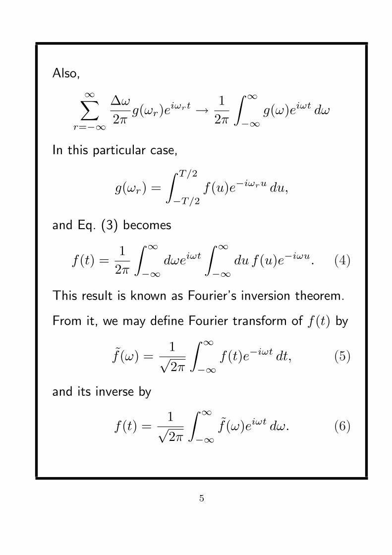
Also,

∞∑r=−∞

∆ω

2πg(ωr)eiωrt → 1

2π

∫ ∞

−∞g(ω)eiωt dω

In this particular case,

g(ωr) =∫ T/2

−T/2

f(u)e−iωru du,

and Eq. (3) becomes

f(t) =12π

∫ ∞

−∞dωeiωt

∫ ∞

−∞du f(u)e−iωu. (4)

This result is known as Fourier’s inversion theorem.

From it, we may define Fourier transform of f(t) by

f̃(ω) =1√2π

∫ ∞

−∞f(t)e−iωt dt, (5)

and its inverse by

f(t) =1√2π

∫ ∞

−∞f̃(ω)eiωt dω. (6)

5

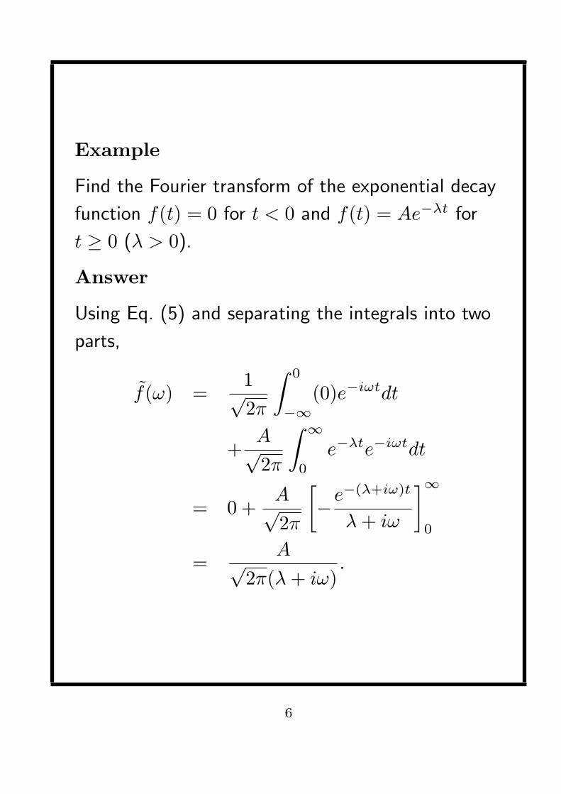
Example

Find the Fourier transform of the exponential decay

function f(t) = 0 for t < 0 and f(t) = Ae−λt for

t ≥ 0 (λ > 0).

Answer

Using Eq. (5) and separating the integrals into two

parts,

f̃(ω) =1√2π

∫ 0

−∞(0)e−iωtdt

+A√2π

∫ ∞

0

e−λte−iωtdt

= 0 +A√2π

[−e−(λ+iω)t

λ + iω

]∞

0

=A√

2π(λ + iω).

6

Dirac δ-function

The δ-function can be visualized as a very sharp

narrow pulse (in space, time, density, etc) which

produces an integrated effect of definite magnitude.

The Dirac δ-function has the property that

δ(t) = 0 for t 6= 0, (7)

but its fundamental defining property is∫

f(t)δ(t− a) dt = f(a) (8)

provided the range of integration includes the point

t = a; otherwise the integral equals zero. This leads

to two further results:∫ b

−a

δ(t) dt = 1 for all a, b > 0 (9)

and ∫δ(t− a) dt = 1 (10)

provided the range of integration includes t = a.

7

Eq. (8) can be used to derive further useful

properties of the Dirac δ-function:

δ(t) = δ(−t) (11)

δ(at) =1|a|δ(t) (12)

tδ(t) = 0. (13)

8

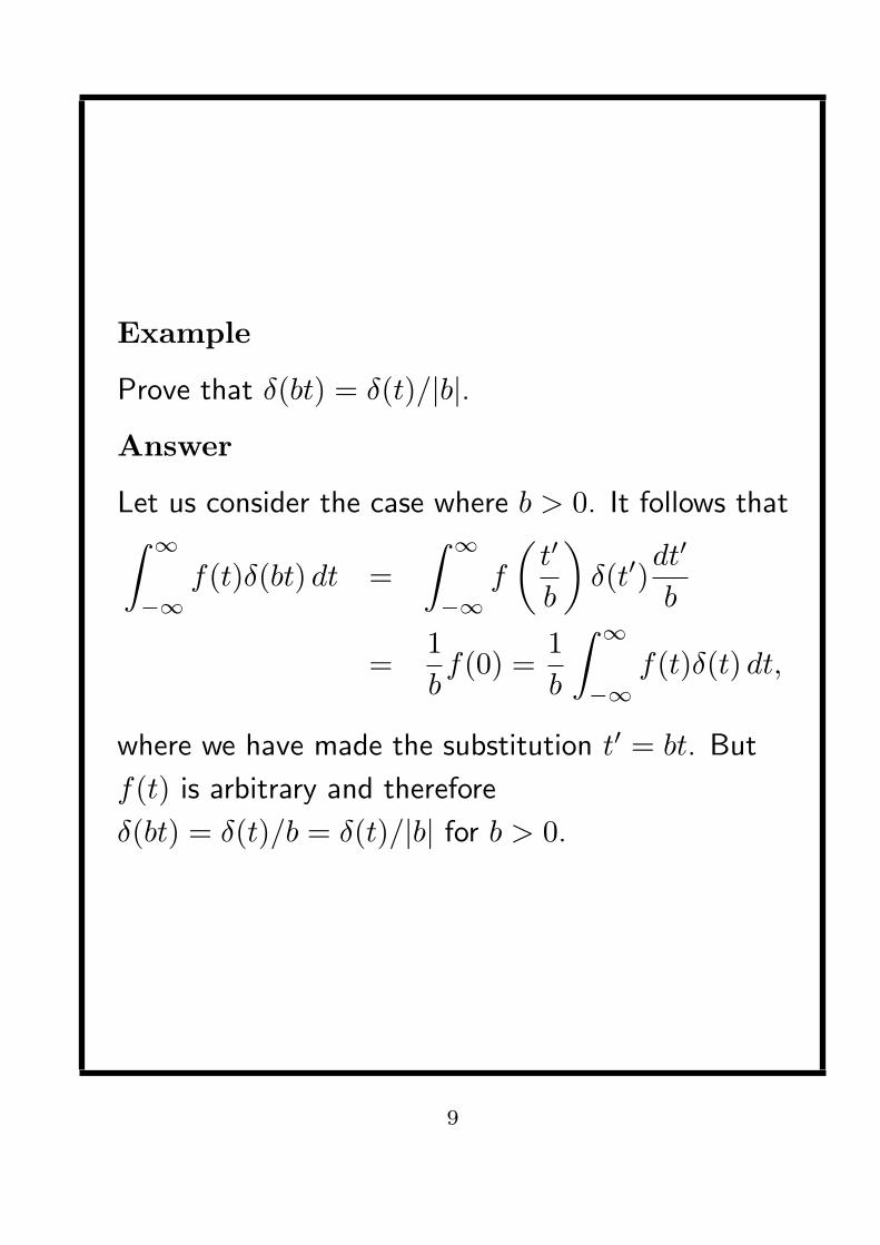
Example

Prove that δ(bt) = δ(t)/|b|.Answer

Let us consider the case where b > 0. It follows that∫ ∞

−∞f(t)δ(bt) dt =

∫ ∞

−∞f

(t′

b

)δ(t′)

dt′

b

=1bf(0) =

1b

∫ ∞

−∞f(t)δ(t) dt,

where we have made the substitution t′ = bt. But

f(t) is arbitrary and therefore

δ(bt) = δ(t)/b = δ(t)/|b| for b > 0.

9

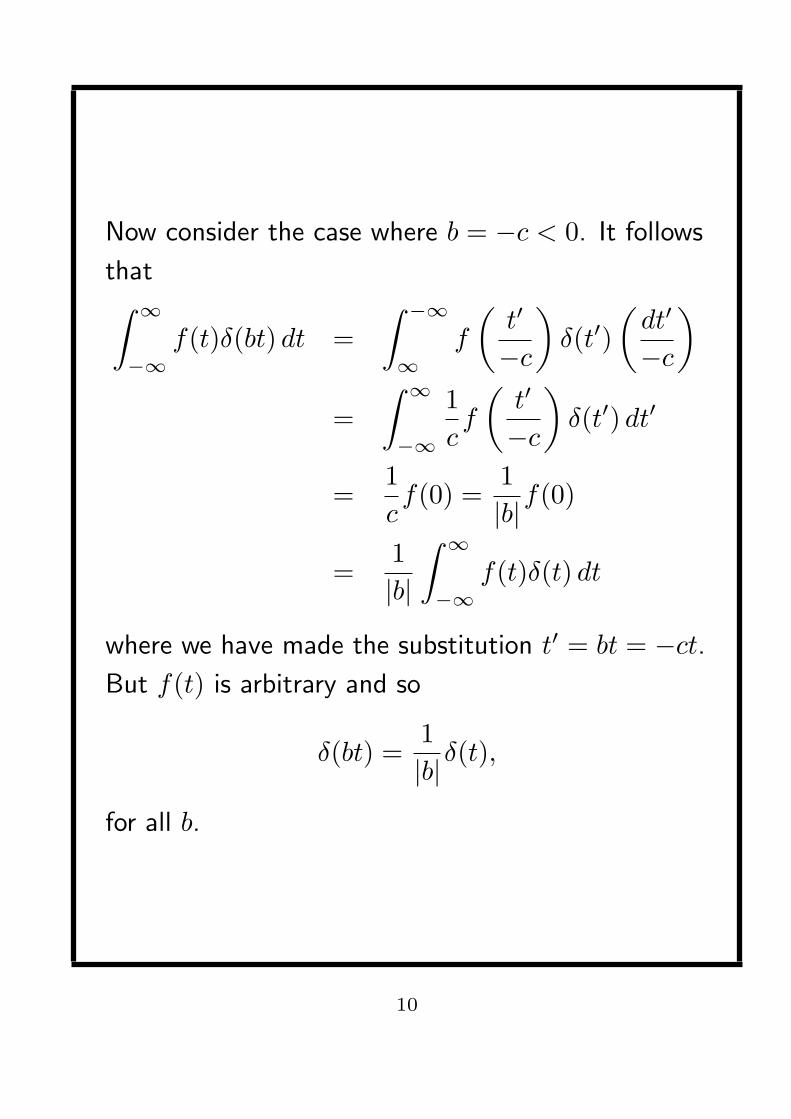
Now consider the case where b = −c < 0. It follows

that∫ ∞

−∞f(t)δ(bt) dt =

∫ −∞

∞f

(t′

−c

)δ(t′)

(dt′

−c

)

=∫ ∞

−∞

1cf

(t′

−c

)δ(t′) dt′

=1cf(0) =

1|b|f(0)

=1|b|

∫ ∞

−∞f(t)δ(t) dt

where we have made the substitution t′ = bt = −ct.

But f(t) is arbitrary and so

δ(bt) =1|b|δ(t),

for all b.

10

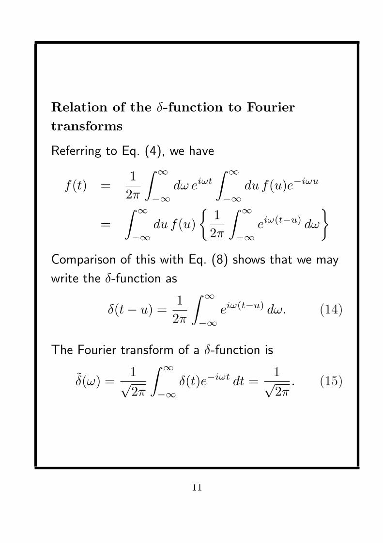
Relation of the δ-function to Fouriertransforms

Referring to Eq. (4), we have

f(t) =12π

∫ ∞

−∞dω eiωt

∫ ∞

−∞du f(u)e−iωu

=∫ ∞

−∞du f(u)

{12π

∫ ∞

−∞eiω(t−u) dω

}

Comparison of this with Eq. (8) shows that we may

write the δ-function as

δ(t− u) =12π

∫ ∞

−∞eiω(t−u) dω. (14)

The Fourier transform of a δ-function is

δ̃(ω) =1√2π

∫ ∞

−∞δ(t)e−iωt dt =

1√2π

. (15)

11

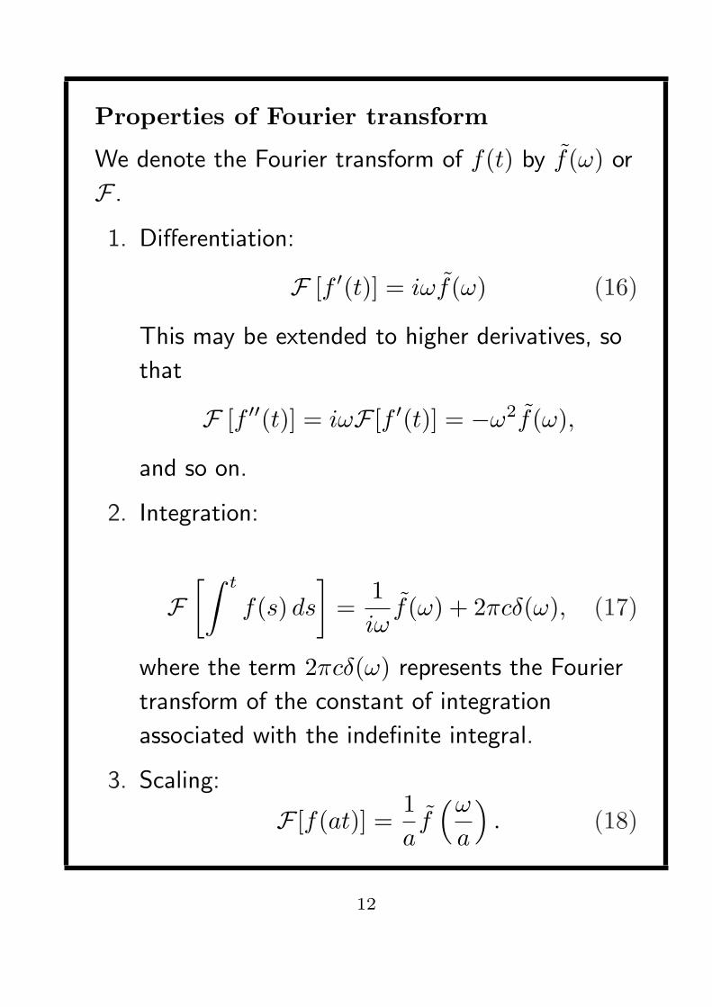
Properties of Fourier transform

We denote the Fourier transform of f(t) by f̃(ω) or

F .

1. Differentiation:

F [f ′(t)] = iωf̃(ω) (16)

This may be extended to higher derivatives, so

that

F [f ′′(t)] = iωF [f ′(t)] = −ω2f̃(ω),

and so on.

2. Integration:

F[∫ t

f(s) ds

]=

1iω

f̃(ω) + 2πcδ(ω), (17)

where the term 2πcδ(ω) represents the Fourier

transform of the constant of integration

associated with the indefinite integral.

3. Scaling:

F [f(at)] =1af̃

(ω

a

). (18)

12

4. Translation:

F [f(t + a)] = eiaω f̃(ω). (19)

5. Exponential multiplication:

F [eαtf(t)

]= f̃(ω + iα), (20)

where α may be real, imaginary or complex.

13

Example

Prove relation F [f ′(t)] = iωf̃(ω).

Answer

Calculating the Fourier transform of f ′(t) directly,

we obtain

F [f ′(t)] =1√2π

∫ ∞

−∞f ′(t)e−iωt dt

=1√2π

[e−iωtf(t)

]∞−∞

+1√2π

∫ ∞

−∞iωe−iωtf(t) dt

= iωf̃(ω),

if f(t) → 0 at t = ±∞ (as it must since∫∞−∞ |f(t)| dt is finite).

14

Odd and even functions

Let us consider an odd function f(t) = −f(−t),whose Fourier transform is given by

f̃(ω) =1√2π

∫ ∞

−∞f(t)e−iωt dt

=1√2π

∫ ∞

−∞f(t)(cos ωt− i sin ωt) dt

=−2i√

2π

∫ ∞

0

f(t) sin ω dt,

since f(t) and sin ωt are odd, whereas cosωt is

even.

We note that f̃(−ω) = −f̃(ω), i.e. f̃(ω) is an odd

function of ω.

15

Hence

f(t) =1√2π

∫ ∞

−∞f̃(ω)eiωt dω

=2i√2π

∫ ∞

0

f̃(ω) sin ωt dω

=2π

∫ ∞

0

dω sin ωt

{∫ ∞

0

f(u) sin ωu du

}.

Thus we may define the Fourier sine transform pair

for odd functions:

f̃s(ω) =

√2π

∫ ∞

0

f(t) sin ωt dt, (21)

f(t) =

√2π

∫ ∞

0

f̃s(ω) sin ωt dω. (22)

16

Convolution and deconvolution

The convolution of the functions f and g is defined

as

h(z) =∫ ∞

−∞f(x)g(z − x) dx (23)

and is often written as f ∗ g.

The convolution is commutative (f ∗ g = g ∗ f),

associative and distributive.

17

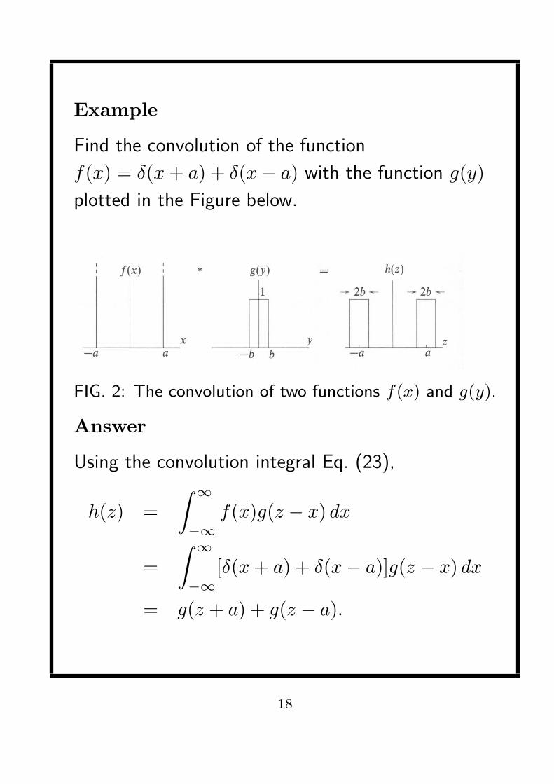
Example

Find the convolution of the function

f(x) = δ(x + a) + δ(x− a) with the function g(y)plotted in the Figure below.

FIG. 2: The convolution of two functions f(x) and g(y).

Answer

Using the convolution integral Eq. (23),

h(z) =∫ ∞

−∞f(x)g(z − x) dx

=∫ ∞

−∞[δ(x + a) + δ(x− a)]g(z − x) dx

= g(z + a) + g(z − a).

18

Let us now consider the Fourier transform of the

convolution [Eq. (23)], which is given by

h̃(k) =1√2π

∫ ∞

−∞dz e−ikz

{∫ ∞

−∞f(x)g(z − x) dx

}

=1√2π

∫ ∞

−∞dxf(x)

{∫ ∞

−∞g(z − x)e−ikz dz

}

If we let u = z − x in the second integral we have

h̃(k) =1√2π

∫ ∞

−∞dxf(x)

{∫ ∞

−∞g(u)e−ik(u+x) du

}

=1√2π

∫ ∞

−∞f(x)e−ikxdx

∫ ∞

−∞g(u)e−iku du

=1√2π

×√

2πf̃(k)×√

2πg̃(k)

=√

2πf̃(k)g̃(k). (24)

19

Hence the Fourier transform of a convolution is

equal to the product of the separate Fourier

transforms multiplied by√

2π; this is called the

convolution theorem.

The converse is also true, namely, that the Fourier

transform of the product f(x)g(x) is given by

F [f(x)g(x)] =1√2π

f̃(k) ∗ g̃(k). (25)

20

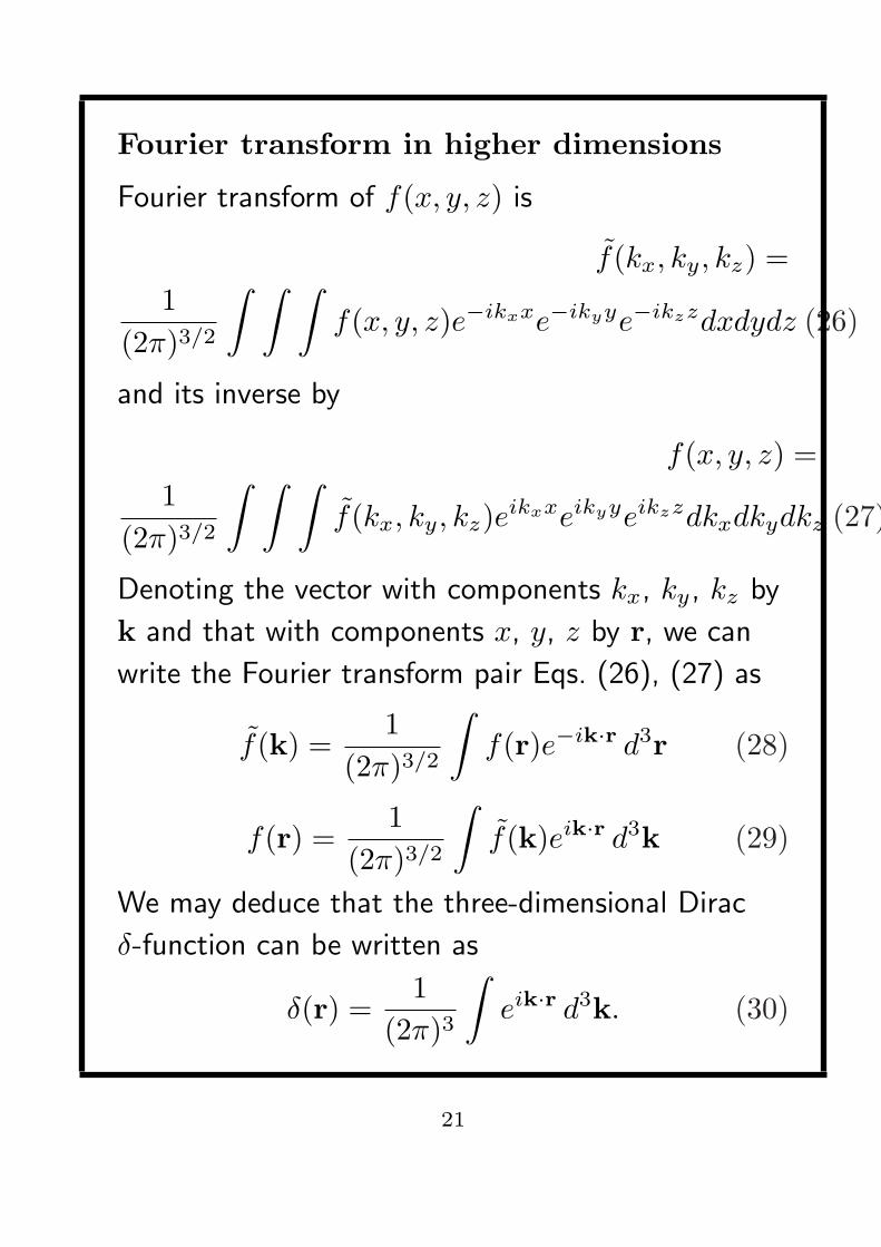
Fourier transform in higher dimensions

Fourier transform of f(x, y, z) is

f̃(kx, ky, kz) =1

(2π)3/2

∫ ∫ ∫f(x, y, z)e−ikxxe−ikyye−ikzzdxdydz (26)

and its inverse by

f(x, y, z) =1

(2π)3/2

∫ ∫ ∫f̃(kx, ky, kz)eikxxeikyyeikzzdkxdkydkz (27)

Denoting the vector with components kx, ky, kz by

k and that with components x, y, z by r, we can

write the Fourier transform pair Eqs. (26), (27) as

f̃(k) =1

(2π)3/2

∫f(r)e−ik·r d3r (28)

f(r) =1

(2π)3/2

∫f̃(k)eik·r d3k (29)

We may deduce that the three-dimensional Dirac

δ-function can be written as

δ(r) =1

(2π)3

∫eik·r d3k. (30)

21