1

Integrable Systems, gradient flows and dissipation

Anthony Bloch(Recent work with Morrison and Ratiu)

•Toda and gradient flows

• Normal and Kahler metrics

• PDE’s on S1 and Loop groups

• Metriplectic Flows

• Double bracket dissipation (w. Jerry, Krishna, Tudor)

2

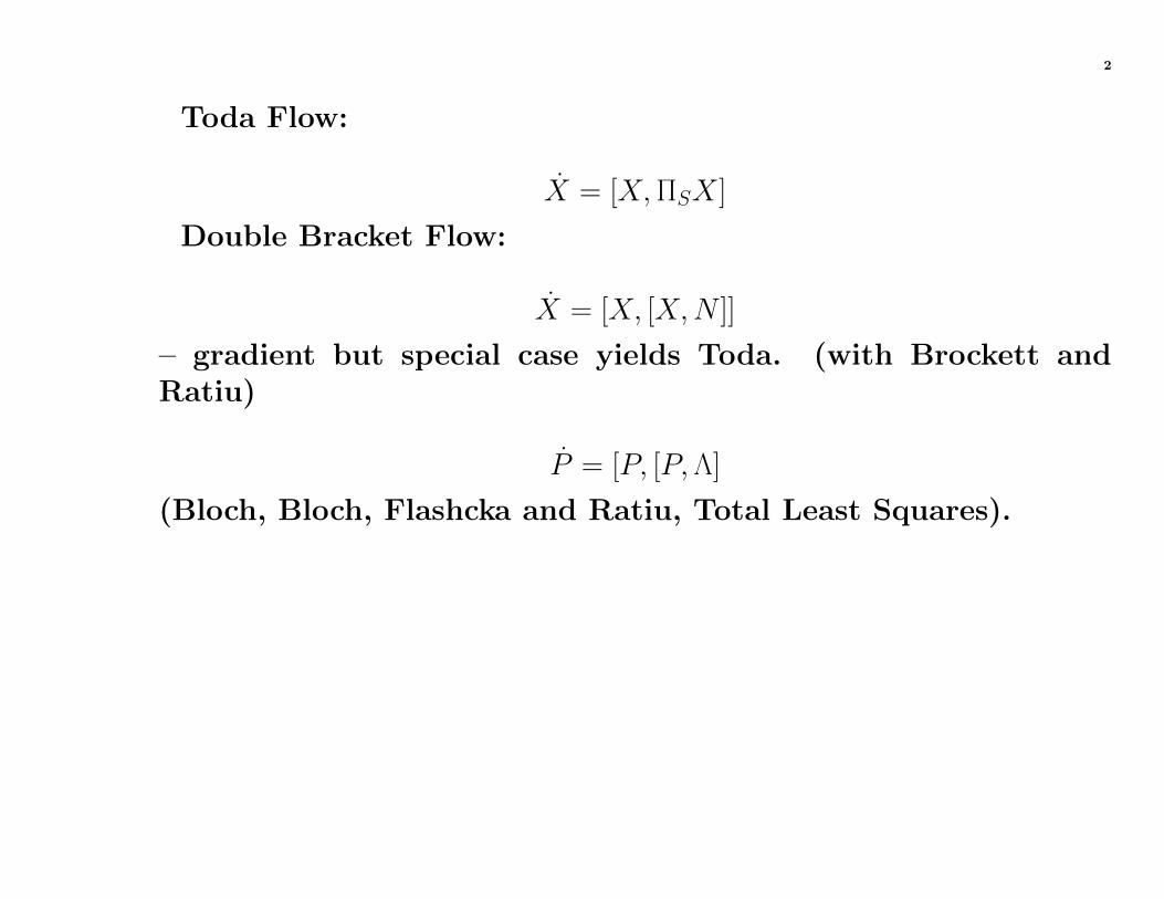
Toda Flow:

X = [X,ΠSX ]

Double Bracket Flow:

X = [X, [X,N ]]

– gradient but special case yields Toda. (with Brockett andRatiu)

P = [P, [P,Λ]

(Bloch, Bloch, Flashcka and Ratiu, Total Least Squares).

3

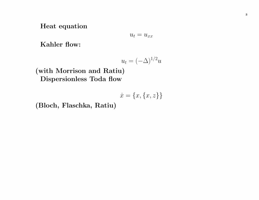
Heat equationut = uxx

Kahler flow:

ut = (−∆)1/2u

(with Morrison and Ratiu)Dispersionless Toda flow

x = x, x, z(Bloch, Flaschka, Ratiu)

4

An important and beautiful mechanical system that describesthe interaction of particles on the line (i.e., in one dimension) isthe Toda lattice. We shall describe the nonperiodic finite Todalattice following the treatment of Moser.

This is a key example in integrable systems theory.The model consists of n particles moving freely on the x-axis

and interacting under an exponential potential. Denoting theposition of the kth particle by xk, the Hamiltonian is given by

H(x, y) =1

2

n∑k=1

y2k +

n−1∑k=1

e(xk−xk+1).

5

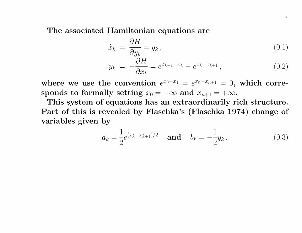
The associated Hamiltonian equations are

xk =∂H

∂yk= yk , (0.1)

yk = −∂H∂xk

= exk−1−xk − exk−xk+1 , (0.2)

where we use the convention ex0−x1 = exn−xn+1 = 0, which corre-sponds to formally setting x0 = −∞ and xn+1 = +∞.

This system of equations has an extraordinarily rich structure.Part of this is revealed by Flaschka’s (Flaschka 1974) change ofvariables given by

ak =1

2e(xk−xk+1)/2 and bk = −1

2yk . (0.3)

6

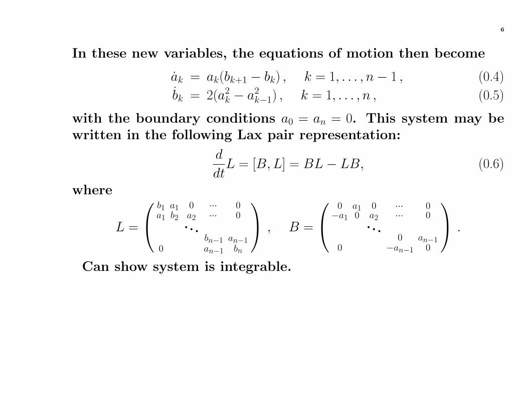
In these new variables, the equations of motion then become

ak = ak(bk+1 − bk) , k = 1, . . . , n− 1 , (0.4)

bk = 2(a2k − a2k−1) , k = 1, . . . , n , (0.5)

with the boundary conditions a0 = an = 0. This system may bewritten in the following Lax pair representation:

d

dtL = [B,L] = BL− LB, (0.6)

where

L =

b1 a1 0 ··· 0a1 b2 a2 ··· 0

...bn−1 an−1

0 an−1 bn

, B =

0 a1 0 ··· 0−a1 0 a2 ··· 0

...0 an−1

0 −an−1 0

.

Can show system is integrable.

7

More structure in this example. For instance, if N is the matrixdiag[1, 2, . . . , n], the Toda flow (0.6) may be written in the followingdouble bracket form:

L = [L, [L,N ]] . (0.7)

See Bloch [1990], Bloch, Brockett and Ratiu [1990], and Bloch,Flaschka and Ratiu [1990]. This double bracket equation re-stricted to a level set of the integrals is in fact the gradient flowof the function TrLN with respect to the so-called normal metric.

From this observation it is easy to show that the flow tendsasymptotically to a diagonal matrix with the eigenvalues of L(0)on the diagonal and ordered according to magnitude, recoveringthe observation of Moser, Symes.

8

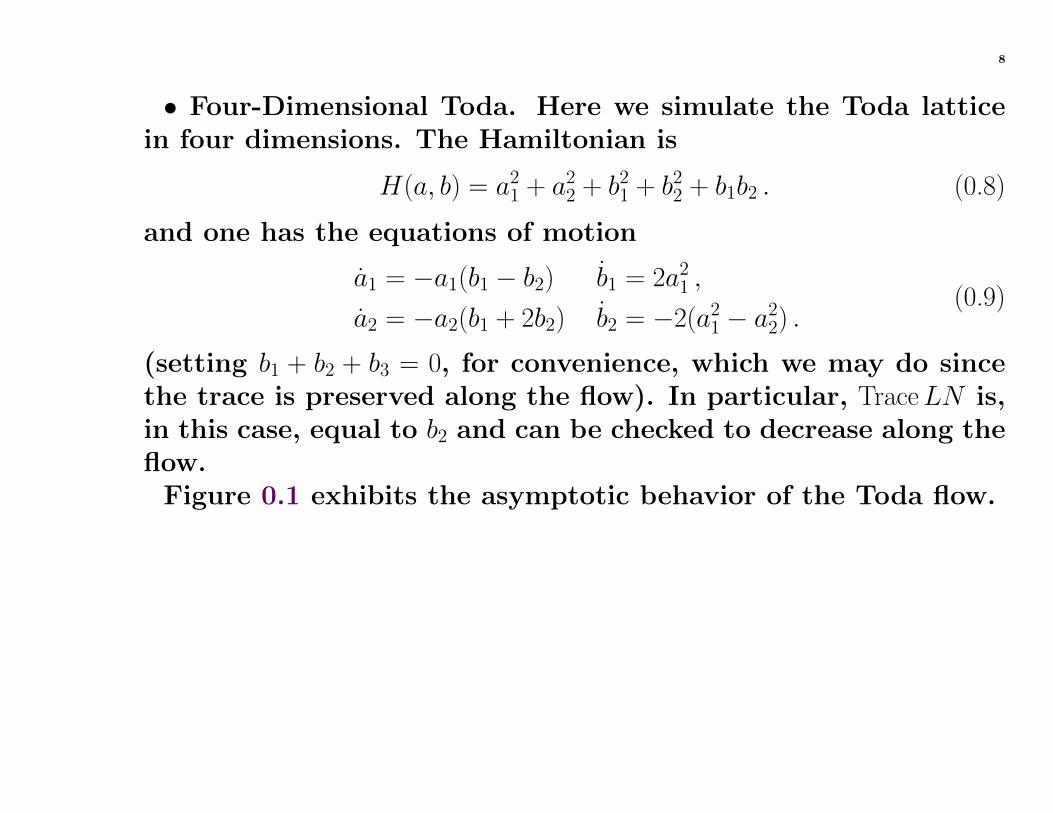
• Four-Dimensional Toda. Here we simulate the Toda latticein four dimensions. The Hamiltonian is

H(a, b) = a21 + a22 + b21 + b22 + b1b2 . (0.8)

and one has the equations of motion

a1 = −a1(b1 − b2) b1 = 2a21 ,

a2 = −a2(b1 + 2b2) b2 = −2(a21 − a22) .(0.9)

(setting b1 + b2 + b3 = 0, for convenience, which we may do sincethe trace is preserved along the flow). In particular, TraceLN is,in this case, equal to b2 and can be checked to decrease along theflow.

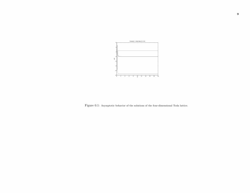
Figure 0.1 exhibits the asymptotic behavior of the Toda flow.

9

0 2 4 6 8 10 12 14 16 18 20−8

−6

−4

−2

0

2

4

6

t

a,b

Example 1, initial data [1,2,3,4]

Figure 0.1: Asymptotic behavior of the solutions of the four-dimensional Toda lattice.

10

It is also of interest to note that the Toda flow may be writ-ten as a different double bracket flow on the space of rank oneprojection matrices. The idea is to represent the flow in the vari-ables λ = (λ1, λ2, . . . , λn) and r = (r1, r2, . . . , rn) where the λi are the(conserved) eigenvalues of L and ri,

∑i r

2i = 1 are the top com-

ponents of the normalized eiqenvectors of L (see Moser). Thenone can show (Bloch (1990)) that the flow may be written as

P = [P, [P,Λ]] (0.10)

where P = rrT and Λ = diag(λ).This flow is a flow on a simplex The Toda flow in its original

variables can also be mapped to a flow convex polytope (seeBloch, Brockett and Ratiu, Bloch, Flaschka and Ratiu).

11

Schur Horn Polytope

(1,2,3)

Figure 0.2: Image of Toda Flow

12

Metrics on finite-dimensional orbitsLet gu be the compact real form of a complex semisimple Lie

algebra g and consider the flow on an adjoint orbit of gu givenby

L(t) = [L(t), [L(t), N ]] . (0.11)

Consider the gradient flow with respect to the “normal” metric(see Atiyah ). Explicitly this metric is given as follows.

Decompose orthogonally, relative to −κ( , ) = 〈 , 〉, gu = gLu⊕guLwhere guL is the centralizer of L and gLu = Im adL. For X ∈ gudenote by XL ∈ gLu the orthogonal projection of X on gLu . Thenset the inner product of the tangent vectors [L,X ] and [L, Y ] tobe equal to 〈XL, Y L〉. Denote this metric by 〈 , 〉N . Then wehave

13

Proposition 0.1. The flow (0.11) is the gradient vector field of H(L) =κ(L,N), κ the Killing form, on the adjoint orbit O of gu containing theinitial condition L(0) = L0, with respect to the normal metric 〈 , 〉N onO.

Proof. We have, by the definition of the gradient,

dH · [L, δL] = 〈gradH, [L, δL]〉N (0.12)

where · denotes the natural pairing between 1-forms and tangent vectors and[L, δL] is a tangent vector at L. Set gradH = [L,X ]. Then (0.12) becomes

−〈[L, δL], N〉 = 〈[L,X ], [L, δL]〉Nor

〈[L,N ], δL〉 = 〈XL, δLL〉 .Thus

XL = ([L,N ])L = [L,N ]

14

andgradH = [L, [L,N ]]

as required.

For L and N as above obtain the Toda lattice flow. Full Todamay be also obtained with a modified metric.

15

Now in addition to the normal metric on an orbit there existtwo other natural metrics, the induced and Kahler metrics.• There is the natural metric b on G/T induced from the invari-

ant metric on the Lie algebra –this is the induced metric.• There is the normal metric described above which, following

Atiyah we call b1, which comes from viewing G/T as an adjointorbit.• Finally identifying the adjoint orbit with a coadjoint orbit we

obtain the Kostant Kirilov symplectic structure which, togetherthe fact that G/T is a complex manifold defines a Kahler metricb2.

If we define b1 and b2 in terms of positive self-adjoint operatorsA1 and A2, A1 = A2

2. In fact b is just Tr(AB), b1 is Tr(ALBL) andb2 is essentially the square root of b1.

16

Gradient flows on the loop group of the circleRecall that the loop group L(S1) of the circle S1 consists of

smooth maps of S1 to S1. With pointwise multiplication, L(S1)

is a commutative group. Often, elements of L(S1) are written as

eif , where f ∈ L(R) := g : [−π, π]→ R | g is C∞, g(π) = g(−π) + 2nπ,for some n ∈ Z; n is the winding number of the closed curve

[−π, π] 3 t 7→ eig(t) ∈ S1 about the origin.

17

The based loop group of S1. The inner product on the Hilbertspace L2(S1) of L2 real valued functions on S1 is defined by

〈f, g〉 :=1

2π

∫ π

−πf (θ)g(θ)dθ, f, g ∈ L2(S1).

We introduce the closed Hilbert Lie subgroup L(S1) := ϕ ∈L(S1) | ϕ(1) = 1 of L(S1) whose closed commutative Hilbert Liealgebra is L(R) := u ∈ Hs(S1,R) | u(1) = 0. The exponential mapexp : L(R) 3 u 7→ eiu ∈ L(S1) is a Lie group isomorphism (with L(R)thought of as a commutative group relative to addition).

18

There is a natural 2-cocycle ω on L(R), namely

ω(u, v) :=1

2π

∫ π

−πdθ u′(θ)v(θ) = 〈u′, v〉 , (0.13)

where u′ := du/dθ. Therefore, there is a central extension of Liealgebras

0 −→ R −→ L(R) −→ L(R) −→ 0

which, integrates to a central extension of Lie groups

1 −→ S1 −→ L(S1) −→ L(S1) −→ 1.

The “geometric duals” of L(R) and L(R) = R⊕L(R) are themselves,relative to the weak L2-pairing.

19

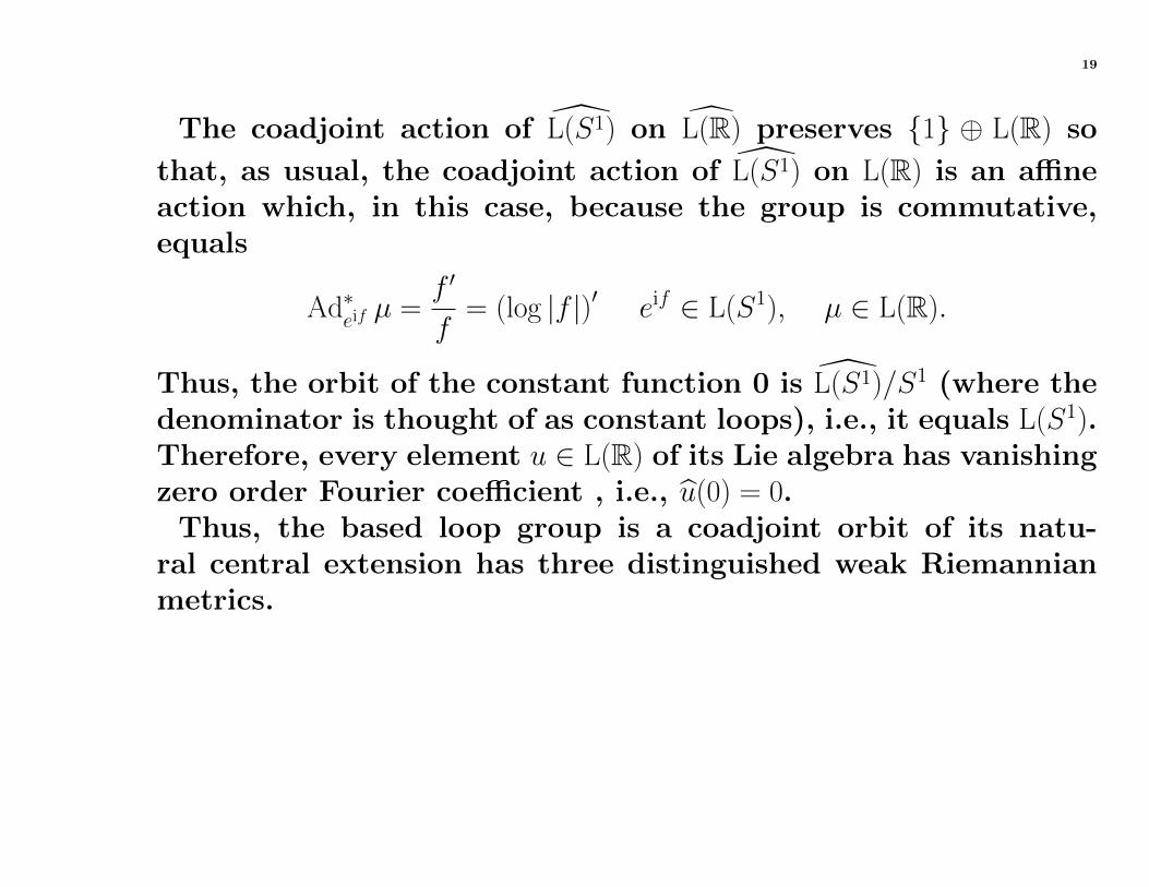
The coadjoint action of L(S1) on L(R) preserves 1 ⊕ L(R) so

that, as usual, the coadjoint action of L(S1) on L(R) is an affineaction which, in this case, because the group is commutative,equals

Ad∗eif µ =f ′

f= (log |f |)′ eif ∈ L(S1), µ ∈ L(R).

Thus, the orbit of the constant function 0 is L(S1)/S1 (where thedenominator is thought of as constant loops), i.e., it equals L(S1).Therefore, every element u ∈ L(R) of its Lie algebra has vanishingzero order Fourier coefficient , i.e., u(0) = 0.

Thus, the based loop group is a coadjoint orbit of its natu-ral central extension has three distinguished weak Riemannianmetrics.

20

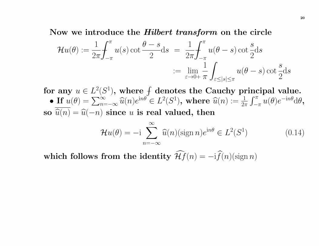
Now we introduce the Hilbert transform on the circle

Hu(θ) :=1

2π−∫ π

−πu(s) cot

θ − s2

ds =1

2π−∫ π

−πu(θ − s) cot

s

2ds

:= limε→0+

1

π

∫ε≤|s|≤π

u(θ − s) cots

2ds

for any u ∈ L2(S1), where −∫

denotes the Cauchy principal value.• If u(θ) =

∑∞n=−∞ u(n)einθ ∈ L2(S1), where u(n) := 1

2π

∫ π−π u(θ)e−inθdθ,

so u(n) = u(−n) since u is real valued, then

Hu(θ) = −i

∞∑n=−∞

u(n)(signn)einθ ∈ L2(S1) (0.14)

which follows from the identity Hf (n) = −if (n)(signn)

21

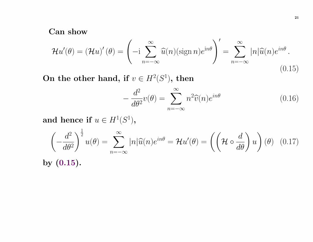
Can show

Hu′(θ) = (Hu)′ (θ) =

(−i

∞∑n=−∞

u(n)(signn)einθ

)′=

∞∑n=−∞

|n|u(n)einθ .

(0.15)On the other hand, if v ∈ H2(S1), then

− d2

dθ2v(θ) =

∞∑n=−∞

n2v(n)einθ (0.16)

and hence if u ∈ H1(S1),(− d2

dθ2

)12

u(θ) =

∞∑n=−∞

|n|u(n)einθ = Hu′(θ) =

((H d

dθ

)u

)(θ) (0.17)

by (0.15).

22

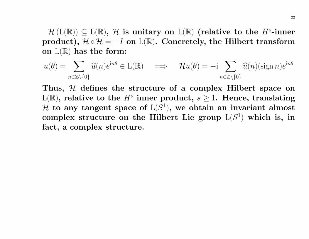
H (L(R)) ⊆ L(R), H is unitary on L(R) (relative to the Hs-innerproduct), HH = −I on L(R). Concretely, the Hilbert transformon L(R) has the form:

u(θ) =∑

n∈Z\0

u(n)einθ ∈ L(R) =⇒ Hu(θ) = −i∑

n∈Z\0

u(n)(signn)einθ

Thus, H defines the structure of a complex Hilbert space onL(R), relative to the Hs inner product, s ≥ 1. Hence, translatingH to any tangent space of L(S1), we obtain an invariant almostcomplex structure on the Hilbert Lie group L(S1) which is, infact, a complex structure.

23

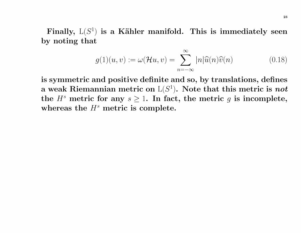
Finally, L(S1) is a Kahler manifold. This is immediately seenby noting that

g(1)(u, v) := ω(Hu, v) =

∞∑n=−∞

|n|u(n)v(n) (0.18)

is symmetric and positive definite and so, by translations, definesa weak Riemannian metric on L(S1). Note that this metric is notthe Hs metric for any s ≥ 1. In fact, the metric g is incomplete,whereas the Hs metric is complete.

24

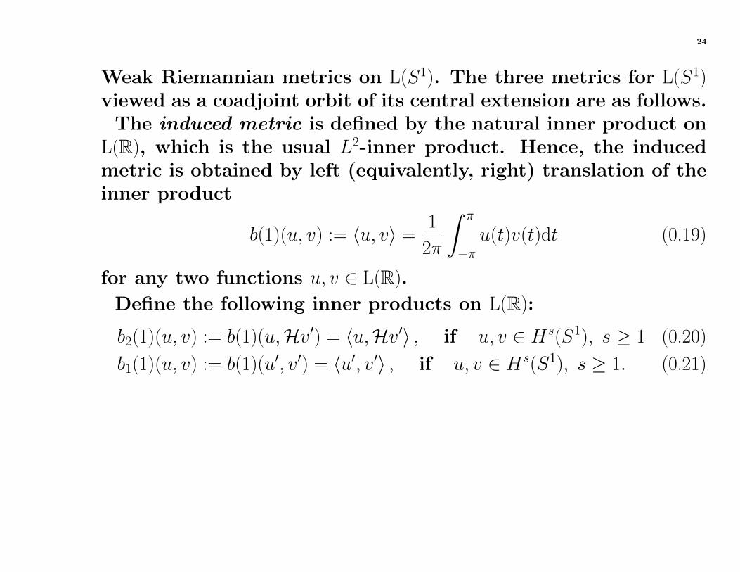
Weak Riemannian metrics on L(S1). The three metrics for L(S1)viewed as a coadjoint orbit of its central extension are as follows.

The induced metric is defined by the natural inner product onL(R), which is the usual L2-inner product. Hence, the inducedmetric is obtained by left (equivalently, right) translation of theinner product

b(1)(u, v) := 〈u, v〉 =1

2π

∫ π

−πu(t)v(t)dt (0.19)

for any two functions u, v ∈ L(R).

Define the following inner products on L(R):

b2(1)(u, v) := b(1)(u,Hv′) = 〈u,Hv′〉 , if u, v ∈ Hs(S1), s ≥ 1 (0.20)

b1(1)(u, v) := b(1)(u′, v′) = 〈u′, v′〉 , if u, v ∈ Hs(S1), s ≥ 1. (0.21)

25

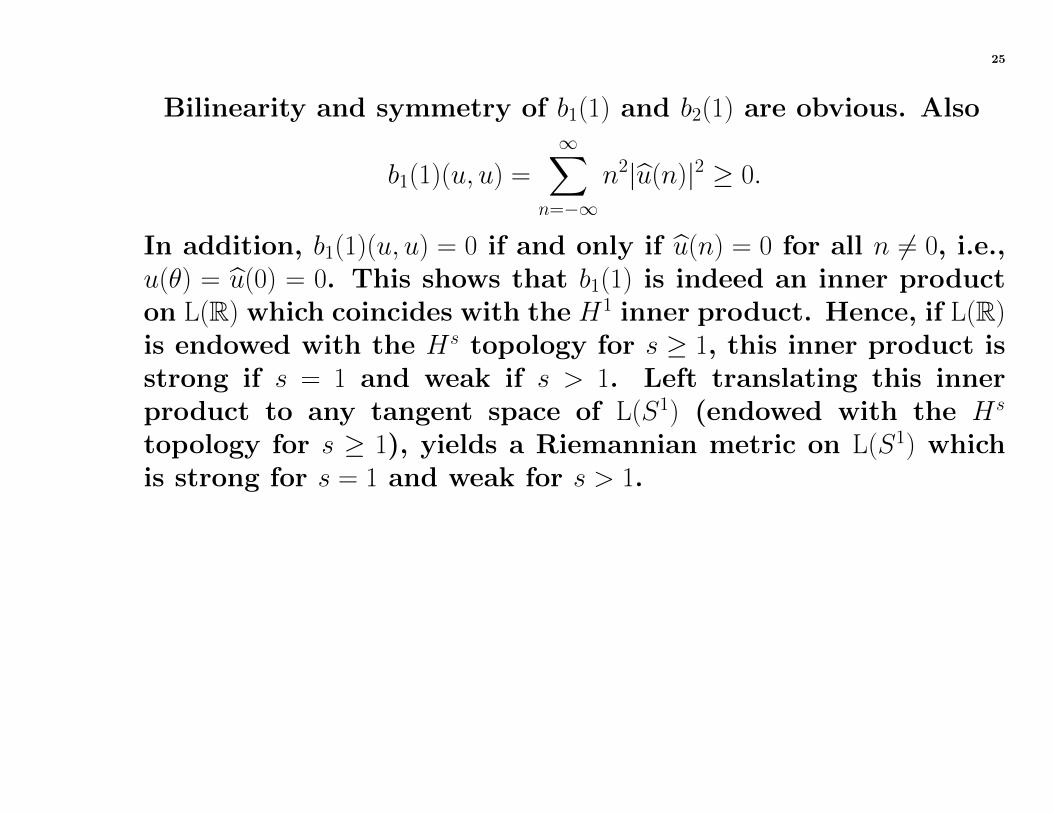
Bilinearity and symmetry of b1(1) and b2(1) are obvious. Also

b1(1)(u, u) =

∞∑n=−∞

n2|u(n)|2 ≥ 0.

In addition, b1(1)(u, u) = 0 if and only if u(n) = 0 for all n 6= 0, i.e.,u(θ) = u(0) = 0. This shows that b1(1) is indeed an inner producton L(R) which coincides with the H1 inner product. Hence, if L(R)is endowed with the Hs topology for s ≥ 1, this inner product isstrong if s = 1 and weak if s > 1. Left translating this innerproduct to any tangent space of L(S1) (endowed with the Hs

topology for s ≥ 1), yields a Riemannian metric on L(S1) whichis strong for s = 1 and weak for s > 1.

26

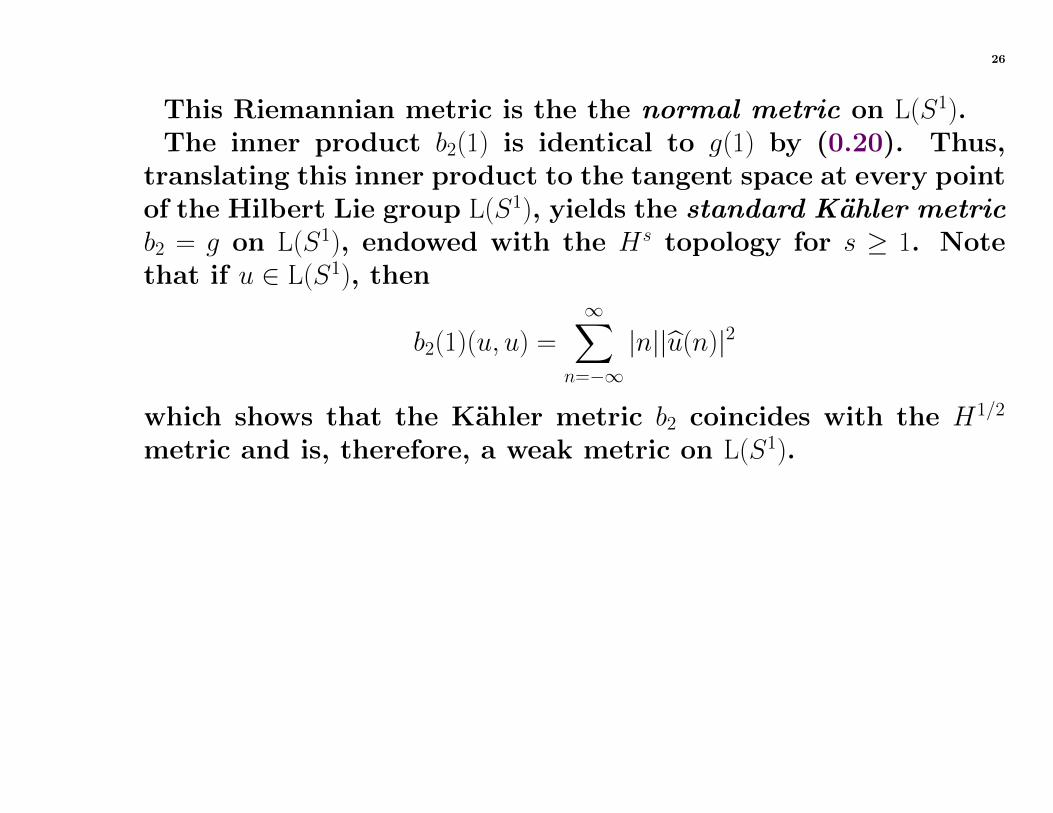
This Riemannian metric is the the normal metric on L(S1).The inner product b2(1) is identical to g(1) by (0.20). Thus,

translating this inner product to the tangent space at every pointof the Hilbert Lie group L(S1), yields the standard Kahler metricb2 = g on L(S1), endowed with the Hs topology for s ≥ 1. Notethat if u ∈ L(S1), then

b2(1)(u, u) =

∞∑n=−∞

|n||u(n)|2

which shows that the Kahler metric b2 coincides with the H1/2

metric and is, therefore, a weak metric on L(S1).

27

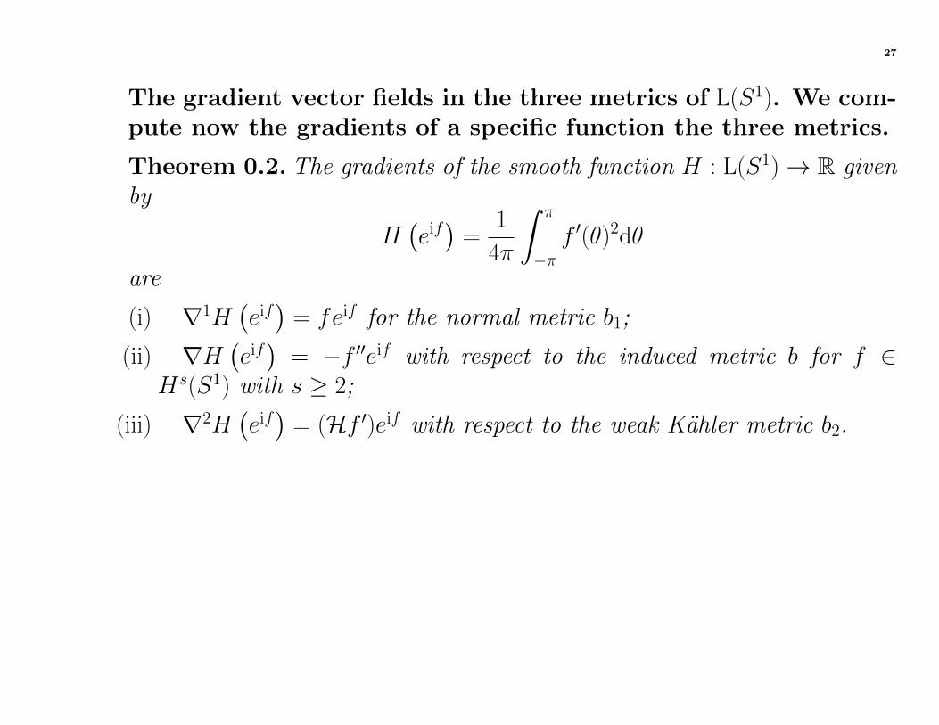
The gradient vector fields in the three metrics of L(S1). We com-pute now the gradients of a specific function the three metrics.

Theorem 0.2. The gradients of the smooth function H : L(S1)→ R givenby

H(eif)

=1

4π

∫ π

−πf ′(θ)2dθ

are

(i) ∇1H(eif)

= feif for the normal metric b1;

(ii) ∇H(eif)

= −f ′′eif with respect to the induced metric b for f ∈Hs(S1) with s ≥ 2;

(iii) ∇2H(eif)

= (Hf ′)eif with respect to the weak Kahler metric b2.

28

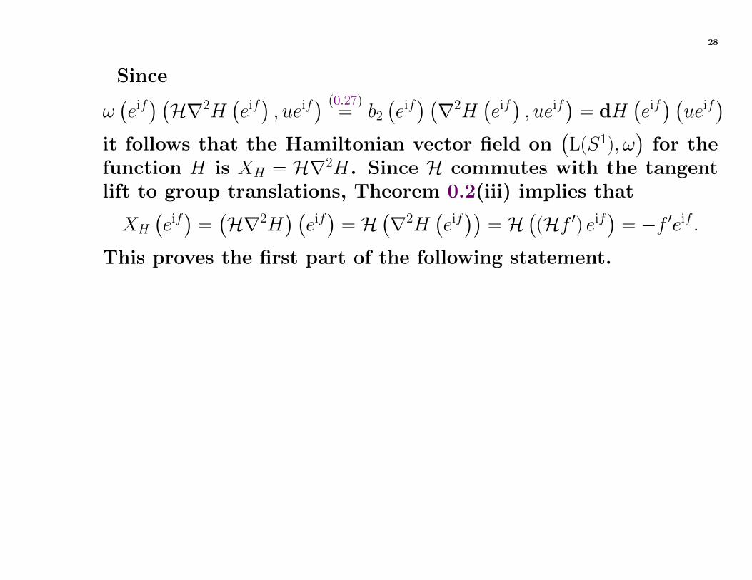
Since

ω(eif) (H∇2H

(eif), ueif

) (0.27)= b2

(eif) (∇2H

(eif), ueif

)= dH

(eif) (ueif

)it follows that the Hamiltonian vector field on

(L(S1), ω

)for the

function H is XH = H∇2H. Since H commutes with the tangentlift to group translations, Theorem 0.2(iii) implies that

XH

(eif)

=(H∇2H

) (eif)

= H(∇2H

(eif))

= H((Hf ′) eif

)= −f ′eif .

This proves the first part of the following statement.

29

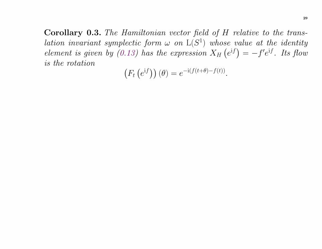
Corollary 0.3. The Hamiltonian vector field of H relative to the trans-lation invariant symplectic form ω on L(S1) whose value at the identityelement is given by (0.13) has the expression XH

(eif)

= −f ′eif . Its flowis the rotation (

Ft(eif))

(θ) = e−i(f(t+θ)−f(t)).

30

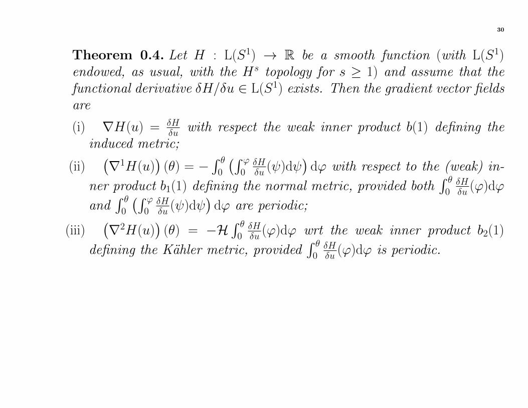
Theorem 0.4. Let H : L(S1) → R be a smooth function (with L(S1)endowed, as usual, with the Hs topology for s ≥ 1) and assume that thefunctional derivative δH/δu ∈ L(S1) exists. Then the gradient vector fieldsare

(i) ∇H(u) = δHδu with respect the weak inner product b(1) defining the

induced metric;

(ii)(∇1H(u)

)(θ) = −

∫ θ0

(∫ ϕ0

δHδu (ψ)dψ

)dϕ with respect to the (weak) in-

ner product b1(1) defining the normal metric, provided both∫ θ0δHδu (ϕ)dϕ

and∫ θ0

(∫ ϕ0

δHδu (ψ)dψ

)dϕ are periodic;

(iii)(∇2H(u)

)(θ) = −H

∫ θ0δHδu (ϕ)dϕ wrt the weak inner product b2(1)

defining the Kahler metric, provided∫ θ0δHδu (ϕ)dϕ is periodic.

31

Vector fields on L(S1) and L(R):Note the exponential map exp : L(R) 3 u 7→ eiu ∈ L(S1) is a Lie

group isomorphismHere, we identified the Lie algebra of S1 with R, even though,

naturally, it is the imaginary axis, the tangent space at 1 ∈ S1 toS1.

Proposition 0.5. Let X ∈ X(L(R)) be an arbitrary vector field . Then itspush-forward to L(S1)) has the expression

(exp∗X)(eiu)

= X(u)eiu

for any u ∈ L(R).

32

Applying Proposition 0.5 to Theorem 0.2, we get the followingresult:

Corollary 0.6. The three gradient vector fields for the smooth functionH1 : L(R)→ R given by

H1(u) =1

4π

∫ π

−πdθ (u′)2

are

(i) ∇1H1(u) = u for the weak inner product b1(1) defining the normalmetric;

(ii) ∇H1(u) = −u′′ for the weak inner product b(1) defining the inducedmetric, where for u ∈ Hs(R) with s ≥ 2;

(iii) ∇2H1(u) = (Hu′) for the weak inner product b2(1) defining the Kahlermetric.

33

Since the exponential map is a Lie group isomorphism and thethree metrics coincide with the respective inner products at theidentity, their left invariance guarantees that the three innerproducts on L(R) correspond to the three invariant metrics onL(S1).

34

Applying Proposition 0.5 to Corollary 0.3, we conclude:

Corollary 0.7. The Hamiltonian vector field of H1 relative to the sym-plectic form ω given by (0.13) has the expression XH(u) = −u′. Its flowis (Ft(u)) (θ) = u(θ − t).

The verification of the statement about the flow is immediate:d

dt(Ft(u)) (θ) =

d

dtu(θ − t) = −u′(θ − t) = (XH (Ft(u))) (θ).

35

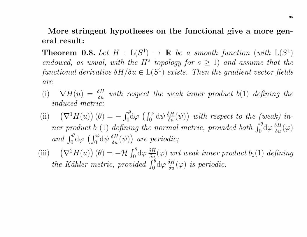
More stringent hypotheses on the functional give a more gen-eral result:

Theorem 0.8. Let H : L(S1) → R be a smooth function (with L(S1)endowed, as usual, with the Hs topology for s ≥ 1) and assume that thefunctional derivative δH/δu ∈ L(S1) exists. Then the gradient vector fieldsare

(i) ∇H(u) = δHδu with respect the weak inner product b(1) defining the

induced metric;

(ii)(∇1H(u)

)(θ) = −

∫ θ0dϕ

(∫ ϕ0 dψ δH

δu (ψ))

with respect to the (weak) in-

ner product b1(1) defining the normal metric, provided both∫ θ0 dϕ δH

δu (ϕ)

and∫ θ0 dϕ

(∫ ϕ0 dψ δH

δu (ψ))

are periodic;

(iii)(∇2H(u)

)(θ) = −H

∫ θ0 dϕ δH

δu (ϕ) wrt weak inner product b2(1) defining

the Kahler metric, provided∫ θ0 dϕ δH

δu (ϕ) is periodic.

36

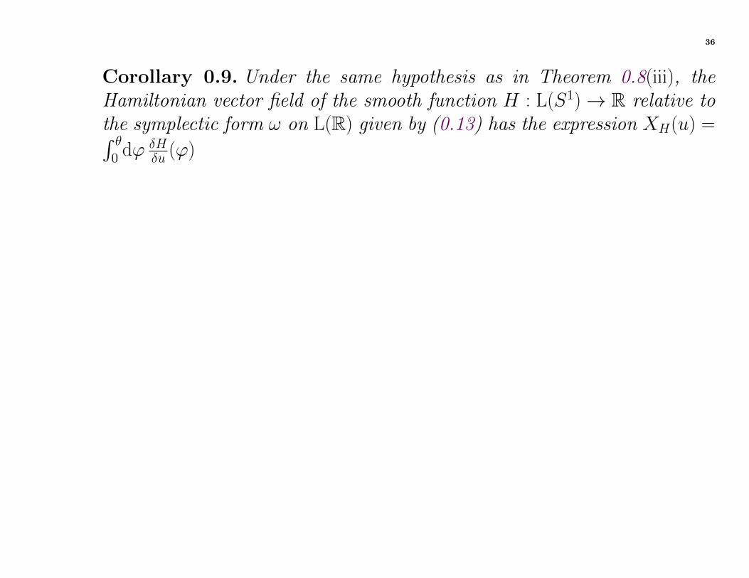
Corollary 0.9. Under the same hypothesis as in Theorem 0.8(iii), theHamiltonian vector field of the smooth function H : L(S1)→ R relative tothe symplectic form ω on L(R) given by (0.13) has the expression XH(u) =∫ θ0 dϕ δH

δu (ϕ)

37

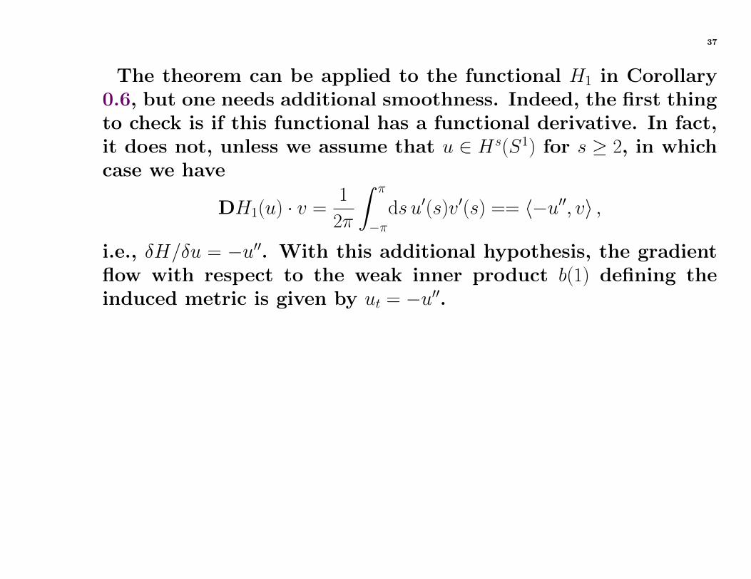
The theorem can be applied to the functional H1 in Corollary0.6, but one needs additional smoothness. Indeed, the first thingto check is if this functional has a functional derivative. In fact,it does not, unless we assume that u ∈ Hs(S1) for s ≥ 2, in whichcase we have

DH1(u) · v =1

2π

∫ π

−πds u′(s)v′(s) == 〈−u′′, v〉 ,

i.e., δH/δu = −u′′. With this additional hypothesis, the gradientflow with respect to the weak inner product b(1) defining theinduced metric is given by ut = −u′′.

38

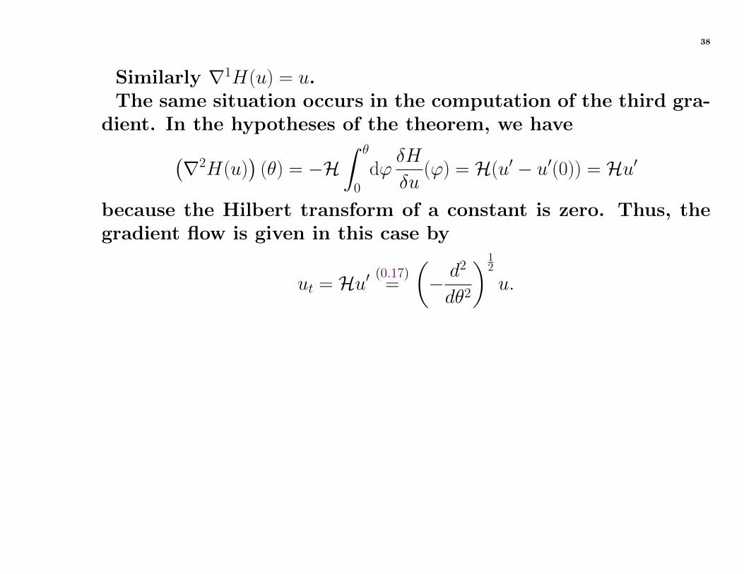
Similarly ∇1H(u) = u.The same situation occurs in the computation of the third gra-

dient. In the hypotheses of the theorem, we have(∇2H(u)

)(θ) = −H

∫ θ

0

dϕδH

δu(ϕ) = H(u′ − u′(0)) = Hu′

because the Hilbert transform of a constant is zero. Thus, thegradient flow is given in this case by

ut = Hu′ (0.17)=

(− d2

dθ2

)12

u.

39

Symplectic structures on loop groups:The periodic Korteweg-de Vries (KdV) equation

ut − 6uuθ + uθθθ = 0, (0.22)

where u(t, θ) is a real valued function of t ∈ R and θ ∈ [−π, π],periodic in θ, and uθ := ∂u/∂θ. The KdV equation is, of course, amost famous integrable Hamiltonian system. It is Hamiltonianon the Poisson manifold of all periodic functions relative to theGardner bracket

F,G =1

2π

∫ π

−πdθδF

δu

d

dθ

δG

δu, (0.23)

where

F (u) =

∫S1

dθ f (u, uθ, uθθ, . . .)

and similarly for G.

40

The functional derivative δF/δu is the usual one relative to theL2(S1) inner product, i.e.,

δF

δu=∂f

∂u− d

dθ

(∂f

∂uθ

)+d2

dθ2

(∂f

∂uθθ

)− · · · .

The Hamiltonian vector field of H(u) = 12π

∫ π−πdθ h(u, uθ, uθθ, . . .) has

the expression

XH(u) =d

dθ

(δH

δu

).

For the KdV equation one takes

H(u) =1

2π

∫ π

−πdθ

(2u3 +

1

2u2θ

). (0.24)

41

The Casimir functions of the Gardner bracket are all smoothfunctionals C for which δC/δu = c is a constant function, i.e.,

C(u) = 〈c, u〉 =1

2π

∫ π

−πdθ cu(θ) = cu(0).

Thus C−1(0) is a candidate weak symplectic leaf in the phase spaceof all periodic functions. The situation in infinite dimensionsis not as clear as in finite dimensions, where this would be aconclusion, because there is no general stratification theoremand one cannot expect, in general, more than a weak symplecticform. However, in our case, this actually holds.

42

This immediately shows that there is a tight relationship withthe symplectic form ω of the complex Hilbert space L(R1) namely

σ

(d2

dθ2u, v

)= ω(u, v)

for all u, v ∈ L(S1) of class Hs, s ≥ 2. Defining(d

dθ

)−1u :=

∫ θ

0

dϕu(ϕ),

the KdV symplectic form σ has the suggestive expression

σ(u1, u2) =

⟨(d

dθ

)−1u1, u2

⟩,

which is well defined on H−12(S1,R).

43

On the other hand, the Poisson bracket given by the Kahlersymplectic form on L(S1) is

F,G =1

2π

∫ π

−πdθδF

δu

(d

dθ

)−1δG

δu, (0.25)

which is similarly well defined on H−12, and the Hamiltonian vec-

tor field defined by this bracket is given by Corollary 0.9, i.e.,

ut = XH(u) =

(d

dθ

)−1δH

δu. (0.26)

Now, the gradient vector field for the corresponding Kahler met-ric, as computed in Theorem 0.8(iii), is written as

ut = −H(d

dθ

)−1δH

δu. (0.27)

44

Metriplectic Systems.A metriplectic system consists of a smooth manifold P , two

smooth vector bundle maps π, κ : T ∗P → TP covering the identity,and two functions H,S ∈ C∞(P ), the Hamiltonian or total energyand the entropy of the system, such that

(i) F,G := 〈dF, π(dG)〉 is a Poisson bracket; in particular π∗ =−π;

(ii) (F,G) := 〈dF, κ(dG)〉 is a positive semidefinite symmetricbracket, i.e., ( , ) is R-bilinear and symmetric, so κ∗ = κ, and(F, F ) ≥ 0 for every F ∈ C∞(P );

(iii) S, F = 0 and (H,F ) = 0 for all F ∈ C∞(P ) ⇐⇒ π(dS) =κ(dH) = 0.

45

The metriplectic dynamics of the system is given in terms ofthe two brackets by

d

dtF = F,H+S+(F,H+S) = F,H+(F, S), for all F ∈ C∞(P ),

(0.28)or, equivalently, as an ordinary differential equation, by

d

dtc(t) = π(c(t))dH(c(t)) + κ(c(t))dS(c(t)). (0.29)

The Hamiltonian vector field XH := π(dH) ∈ X(P ) represents theconservative or Hamiltonian part, whereas YS := κ(dS) ∈ X(P )the dissipative part of the full metriplectic dynamics (0.28) or(0.29).

46

The definition of metriplectic systems has three immediate im-portant consequences. Let c(t) be an integral curve of the system(0.29).

(1) Energy conservation :

d

dtH(c(t)) = H,H(c(t)) + (H,S)(c(t)) = 0. (0.30)

(2) Entropy production :

d

dtS(c(t)) = S,H(c(t)) + (S, S)(c(t)) ≥ 0. (0.31)

(3) Maximum entropy principle yields equilibria : Suppose thatthere are n functions C1, . . . , Cn ∈ C∞(P ) such that F,Ci =(F,Ci) = 0 for all F ∈ C∞(P ), i.e., these functions are simulta-neously conserved by the conservative and dissipative part ofthe metriplectic dynamics.

47

Let p0 ∈ P be a maximum of the entropy S subject to theconstraints H−1(h)∩C−11 (c1)∩ . . . C−1n (cn), for given regular valuesh, c1, . . . , cn ∈ R of H,C1, . . . , Cn, respectively. By the LagrangeMultiplier Theorem, there exist α, β1, . . . , βn ∈ R such that

dS(p0) = αdH(p0) + β1dC1(p0) + · · · + dCn(p0).

But then, assuming that α 6= 0, for every F ∈ C∞(P ), we have

F,H(p0) + (F, S)(p0)

= 〈dF (p0), π(p0) (dH(p0))〉 + 〈dF (p0), κ(p0) (dS(p0))〉 = 0

which means that p0 is an equilibrium of the metriplectic dy-namics (0.28) or (0.29). This is akin to the free energy extrem-ization of thermodynamics, as noted by Morrison and Mielke.

48

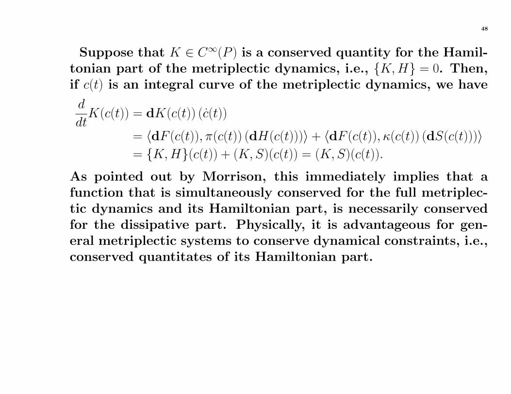
Suppose that K ∈ C∞(P ) is a conserved quantity for the Hamil-tonian part of the metriplectic dynamics, i.e., K,H = 0. Then,if c(t) is an integral curve of the metriplectic dynamics, we have

d

dtK(c(t)) = dK(c(t)) (c(t))

= 〈dF (c(t)), π(c(t)) (dH(c(t)))〉 + 〈dF (c(t)), κ(c(t)) (dS(c(t)))〉= K,H(c(t)) + (K,S)(c(t)) = (K,S)(c(t)).

As pointed out by Morrison, this immediately implies that afunction that is simultaneously conserved for the full metriplec-tic dynamics and its Hamiltonian part, is necessarily conservedfor the dissipative part. Physically, it is advantageous for gen-eral metriplectic systems to conserve dynamical constraints, i.e.,conserved quantitates of its Hamiltonian part.

49

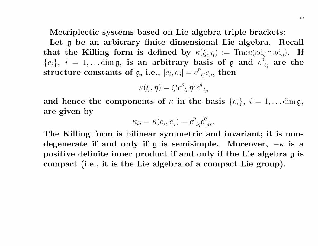
Metriplectic systems based on Lie algebra triple brackets:Let g be an arbitrary finite dimensional Lie algebra. Recall

that the Killing form is defined by κ(ξ, η) := Trace(adξ adη). Ifei, i = 1, . . . dim g, is an arbitrary basis of g and cpij are thestructure constants of g, i.e., [ei, ej] = cpijep, then

κ(ξ, η) = ξicpiqηjcqjp

and hence the components of κ in the basis ei, i = 1, . . . dim g,are given by

κij = κ(ei, ej) = cpiqcqjp.

The Killing form is bilinear symmetric and invariant; it is non-degenerate if and only if g is semisimple. Moreover, −κ is apositive definite inner product if and only if the Lie algebra g iscompact (i.e., it is the Lie algebra of a compact Lie group).

50

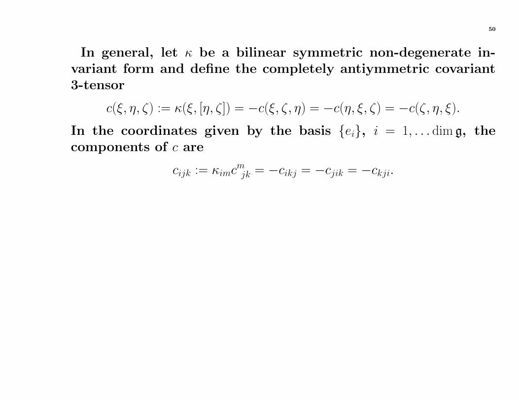
In general, let κ be a bilinear symmetric non-degenerate in-variant form and define the completely antiymmetric covariant3-tensor

c(ξ, η, ζ) := κ(ξ, [η, ζ ]) = −c(ξ, ζ, η) = −c(η, ξ, ζ) = −c(ζ, η, ξ).

In the coordinates given by the basis ei, i = 1, . . . dim g, thecomponents of c are

cijk := κimcmjk = −cikj = −cjik = −ckji.

51

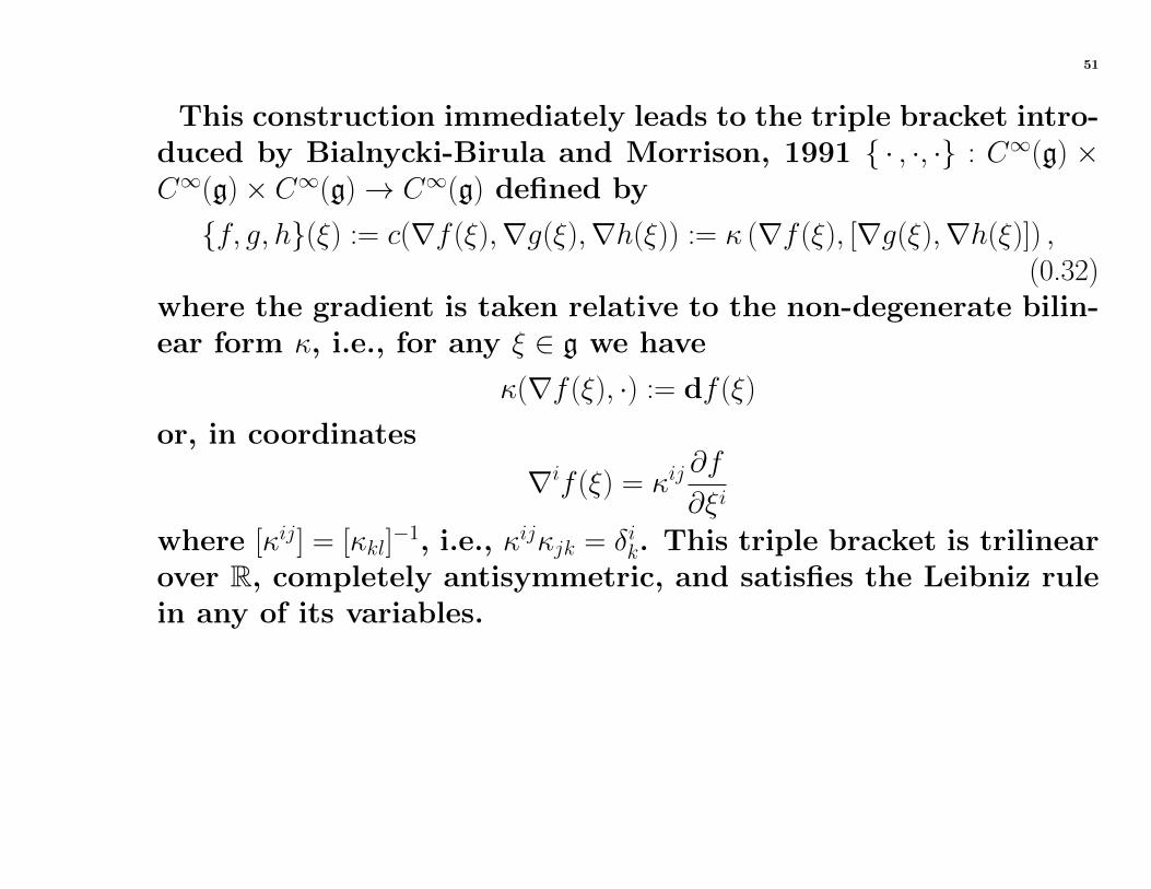
This construction immediately leads to the triple bracket intro-duced by Bialnycki-Birula and Morrison, 1991 · , ·, · : C∞(g) ×C∞(g)× C∞(g)→ C∞(g) defined by

f, g, h(ξ) := c(∇f (ξ),∇g(ξ),∇h(ξ)) := κ (∇f (ξ), [∇g(ξ),∇h(ξ)]) ,(0.32)

where the gradient is taken relative to the non-degenerate bilin-ear form κ, i.e., for any ξ ∈ g we have

κ(∇f (ξ), ·) := df (ξ)

or, in coordinates

∇if (ξ) = κij∂f

∂ξi

where [κij] = [κkl]−1, i.e., κijκjk = δik. This triple bracket is trilinear

over R, completely antisymmetric, and satisfies the Leibniz rulein any of its variables.

52

This construction extends the bracket due to Nambu to a Liealgebra setting. Nambu considered ordinary vectors in R3 anddefined

f, g, hNambu(Π) = ∇f (Π) · (∇g(Π)×∇h(Π)) , (0.33)

where ‘·’ and ‘×’ are the ordinary dot and cross products. Thus,the Nambu bracket is a special case of the triple bracket (0.32) inthe case of g = so(3), whose the structure constants are the com-pletely antisymmetric Levi-Civita symbol εijk. Such ‘modifiedrigid body brackets’ were also described in Bloch and Marsden[1990], Holm and Marsden [1991], and and Marsden and Ratiu[1999].

53

If g is an arbitrary quadratic Lie algebra with bilinear symmet-ric non-degenerate invariant form κ, the quadratic function

C2(ξ) := 12κ(ξ, ξ) (0.34)

is a Casimir function for the Lie-Poisson bracket on g, identifiedwith g∗ via κ, i.e.,

f, g±(ξ) = ±κ (ξ, [∇f (ξ),∇g(ξ)]) , (0.35)

as an easy verification shows since ∇C2(ξ) = ξ. In view of (0.35),the following identity is obvious

f, g+ = C2, f, g.

54

For example, if g = so(3), the (-)Lie-Poisson bracket

f, gso(3)− (Π) = −C2, f, gNambu(Π) = −Π · (∇f (Π)×∇g(Π)) (0.36)

is the rigid body bracket, i.e., if h(Π) = 12Π ·Ω, where Πi = IiΩi,

Ii > 0, i = 1, 2, 3, and Ii are the principal moments of inertia of

the body, then Hamilton’s equations ddtF (Π) = f, hso(3)− (Π) are

equivalent to Euler’s equations Π = Π×Ω.

55

Note that given any two functions, f, g ∈ C∞(g), because thetriple bracket satisfies the Leibniz identity in every factor, themap C∞(g) 3 h 7→ h, f, g ∈ C∞(g) is a derivation and hencedefines a vector field on g, denoted by Xf,g : g→ g, i.e.,

〈dh(ξ), Xf,g(ξ)〉 = κ (∇h(ξ), Xf,g(ξ)) = h, f, g(ξ) for all h ∈ C∞(g).(0.37)

Note that Xf,f = 0. Thus, for triple brackets, two functions definea vector field, analogous to the Hamiltonian vector field definedby a single function associated to a standard Poisson bracket.

56

We have the following result.

Proposition 0.10. The vector field Xf,g on g corresponding to the pair offunctions f, g is given by

Xf,g(ξ) = [∇f (ξ),∇g(ξ)] . (0.38)

57

Triple brackets of the form (0.32) can be used to constructmetriplectic systems on a quadratic Lie algebra g in the followingmanner. Let κ be the bilinear symmetric non-degenerate formon g defining the quadratic structure and fix some h ∈ C∞(g).Define the symmetric bracket

(f, g)κh(ξ) := −κ (Xh,f(ξ), Xh,g(ξ)) . (0.39)

Assume that −κ is a positive definite inner product. Then (f, f ) ≥0. Thus we have the manifold g endowed with the Lie-Poissonbracket (0.35), the symmetric bracket (0.39), the Hamiltonianh, and for the entropy S we take any Casimir function of theLie-Poisson bracket.

58

Then the conditions (i)–(iii) of metriplectic are all satisfied,because (h, g)κh = −κ(Xh,h, Xh,g) = −κ(0, Xh,g) = 0 for any g ∈ C∞(g).The equations of motion (0.28) are in this case given by

d

dtf (ξ) = κ

(∇f (ξ),

d

dtξ

)= f, h±(ξ) + (f, S)(ξ) = ±κ (ξ, [∇f (ξ),∇h(ξ)])− κ (Xh,f(ξ), Xh,S(ξ))

= ∓κ (∇f (ξ), [ξ,∇h(ξ)])− κ ([∇h(ξ),∇f (ξ)], [∇h(ξ),∇S(ξ)])

for any f ∈ C∞(g).This gives the equations of motion

ξ = ±[ξ,∇h(ξ)] + [∇h(ξ), [∇h(ξ),∇S(ξ)]] . (0.40)

59

Note that the flow corresponding to S is a generalized doublebracket flow. Observe also that this flow reduces to a doublebracket flow and is tangent to an orbit of the group if ∇h(ξ) = ξ.Indeed if h = 1

2κ(ξ, ξ) the symmetric bracket (0.39) reduces to thesymmetric bracket induced from the normal metric.

60

Special Case of so(3): If the quadratic Lie algebra is so(3), weidentify it with R3 with the cross product as Lie bracket via theLie algebra isomorphism ˆ : R3 → so(3) given by uv := u × v for

all u,v ∈ R3. Since AdA u = Au, for any A ∈ SO(3) and u ∈ R3, weconclude that the usual inner product on R3 is an invariant innerproduct. In terms of elements of so(3) we have u·v = −1

2 Trace (uv).We shall show below that the metriplectic structure on R3 isprecisely the one given in Morrison [1986].

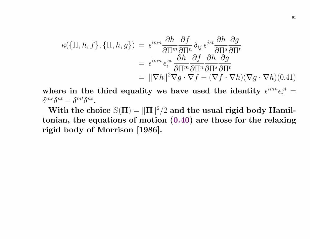
Recall that the Nambu bracket is given for so(3) by (0.33) andhence the symmetric bracket (0.39) has the form

61

κ(Π, h, f, Π, h, g) = εimn∂h

∂Πm

∂f

∂Πnδij ε

jst ∂h

∂Πs

∂g

∂Πt

= εimn ε sti∂h

∂Πm

∂f

∂Πn

∂h

∂Πs

∂g

∂Πt

= ‖∇h‖2∇g · ∇f − (∇f · ∇h)(∇g · ∇h)(0.41)

where in the third equality we have used the identity εimnε sti =δmsδnt − δmtδns.

With the choice S(Π) = ‖Π‖2/2 and the usual rigid body Hamil-tonian, the equations of motion (0.40) are those for the relaxingrigid body of Morrison [1986].

62

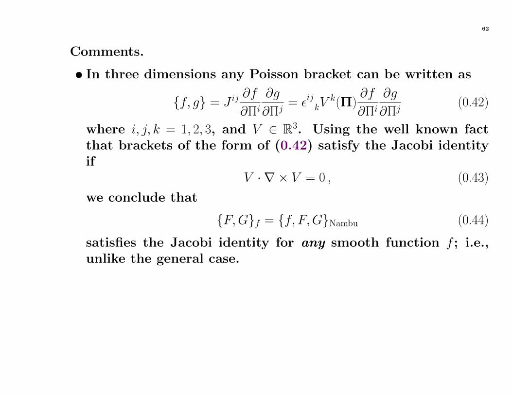
Comments.

• In three dimensions any Poisson bracket can be written as

f, g = J ij∂f

∂Πi

∂g

∂Πj= εijkV

k(Π)∂f

∂Πi

∂g

∂Πj(0.42)

where i, j, k = 1, 2, 3, and V ∈ R3. Using the well known factthat brackets of the form of (0.42) satisfy the Jacobi identityif

V · ∇ × V = 0 , (0.43)

we conclude that

F,Gf = f, F,GNambu (0.44)

satisfies the Jacobi identity for any smooth function f ; i.e.,unlike the general case.

63

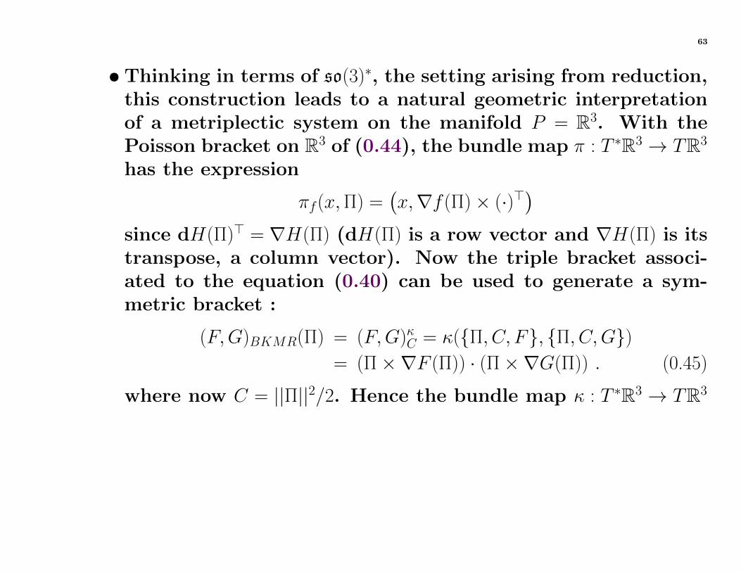
• Thinking in terms of so(3)∗, the setting arising from reduction,this construction leads to a natural geometric interpretationof a metriplectic system on the manifold P = R3. With thePoisson bracket on R3 of (0.44), the bundle map π : T ∗R3 → TR3

has the expression

πf(x,Π) =(x,∇f (Π)× (·)>

)since dH(Π)> = ∇H(Π) (dH(Π) is a row vector and ∇H(Π) is itstranspose, a column vector). Now the triple bracket associ-ated to the equation (0.40) can be used to generate a sym-metric bracket :

(F,G)BKMR(Π) = (F,G)κC = κ(Π, C, F, Π, C,G)= (Π×∇F (Π)) · (Π×∇G(Π)) . (0.45)

where now C = ||Π||2/2. Hence the bundle map κ : T ∗R3 → TR3

64

has the expression

κ(x,Π) = −Π×(Π× (·)>

).

Thus, with the freedom to choose any quantity S = f as an en-tropy, with the assurance that (0.43) will be satisfied because∇ × V = ∇ × ∇f = 0, we can take H = C and have F, Sf = 0and (F,H) = 0 for all F ∈ C∞(R3). The equations of motion forthis metriplectic system are

Π = −Π×∇f (Π)− Π× (Π×∇f (Π)). (0.46)

The symmetric bracket is the inner product of the two Hamil-tonian vector fields on each concentric sphere. As discussedin BKMR, this symmetric bracket can be defined on any com-pact Lie algebra by taking the normal metric on each coadjointorbit.

65

• The following set of equations were given in Fish (2005):

Π = ∇S ×∇H −∇H × (∇H ×∇S). (0.47)

This metriplectic system is equivalent to.

Π = Π, S,H + κ (Π, H,Π, Π, H, S) , (0.48)

(F,G)g(Π) = κ (Π, g, F, Π, g, G) = (∇g(Π)×∇F (Π))·(∇g(Π)×∇G(Π)).(0.49)

Thus, the bundle map κ : T ∗R3 → TR3 has the expression

κg(x,Π) = −∇g(Π)×(∇(Π)× (·)>

).

66

Examples: Two special cases of the equation (0.47) are ofinterest.

(i) If we take H = 12||Π||

2 and S = c · Π, c a constant vector, weobtain

Π = c× Π− Π× (Π× c). (0.50)

(ii) If we take S = 12‖Π‖

2 and H = c ·Π, c a constant, we obtain

Π = Π× c− c× (c× Π) . (0.51)

The equations of motion (0.50) is an instance of double bracketdamping, where the damping is due to the normal metric,whereas (0.51) gives linear damping of the sort arising in quan-tum systems. See also Gay-Balmaz/Holm fluids.

67

Metriplectic extends to full Toda with dissipation:Triple bracket and associate symmetric brackets extends to

fields and PDE’s (see paper.)Related work: dispersionless Toda with Hermann Flaschka and

Tudor.