Initial Analysis in JMulTi · In this model the pair of hypotheses H0: φ = 0 versus H1: φ < 0 is...

Initial Analysis in JMulTiJune 12, 2006

Helmut Lutkepohl, Markus Kratzig

The initial analysis provides a starting point for the time series analysis with JMulTi . It con-

tains plots of important characteristics as summarized in the spectrum and autocorrelation

functions and there are also tests for the order of integration as well as cointegration tests,

which should help choosing an appropriate statistical model. More general tasks, like im-

porting, manipulating and transforming time series, managing data sets, etc. are described

in the help section JMulTi -General Help.

1

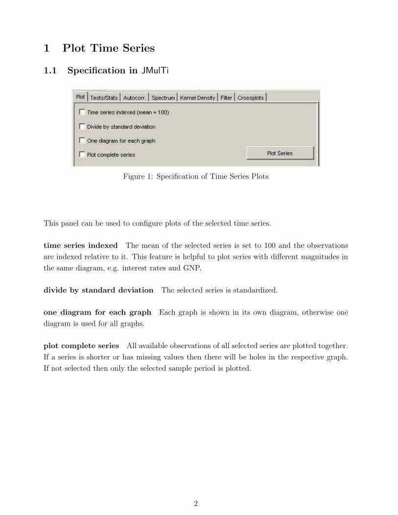
1 Plot Time Series

1.1 Specification in JMulTi

Figure 1: Specification of Time Series Plots

This panel can be used to configure plots of the selected time series.

time series indexed The mean of the selected series is set to 100 and the observations

are indexed relative to it. This feature is helpful to plot series with different magnitudes in

the same diagram, e.g. interest rates and GNP.

divide by standard deviation The selected series is standardized.

one diagram for each graph Each graph is shown in its own diagram, otherwise one

diagram is used for all graphs.

plot complete series All available observations of all selected series are plotted together.

If a series is shorter or has missing values then there will be holes in the respective graph.

If not selected then only the selected sample period is plotted.

2

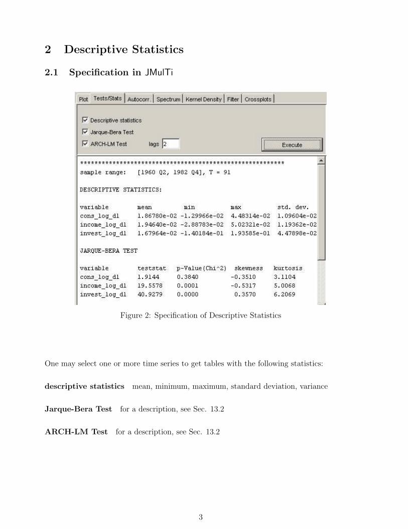
2 Descriptive Statistics


Figure 2: Specification of Descriptive Statistics

One may select one or more time series to get tables with the following statistics:

descriptive statistics mean, minimum, maximum, standard deviation, variance

Jarque-Bera Test for a description, see Sec. 13.2

ARCH-LM Test for a description, see Sec. 13.2

3

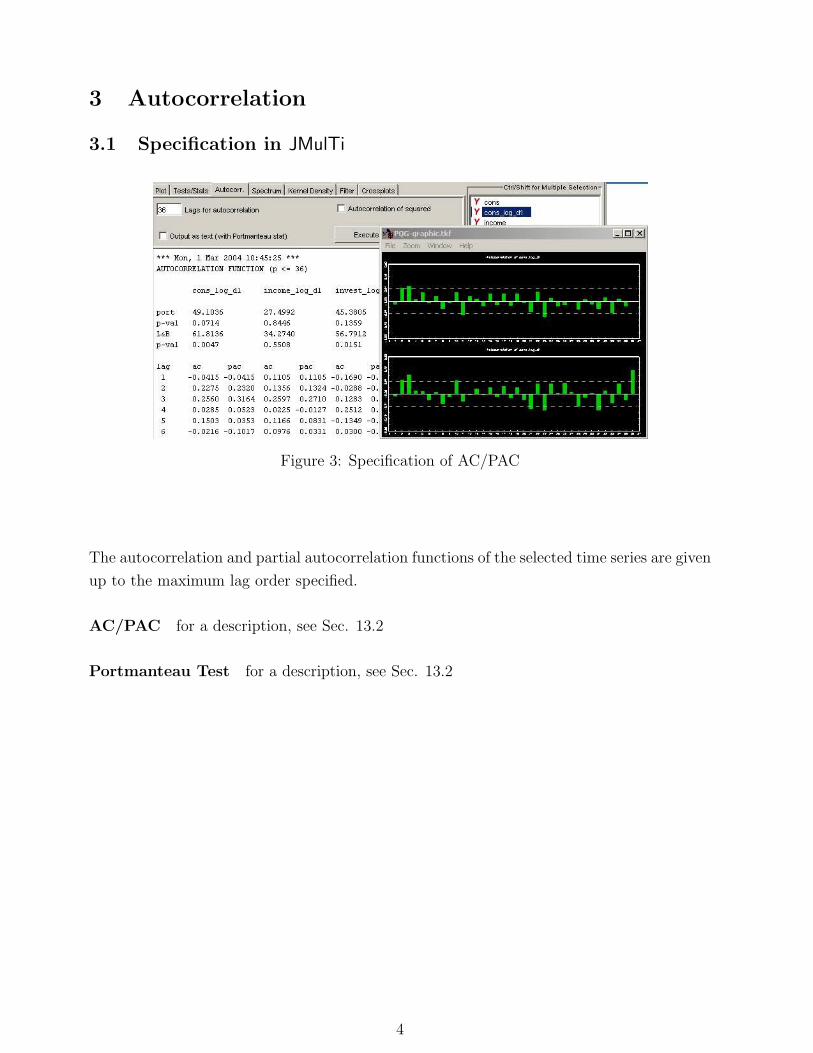
3 Autocorrelation


Figure 3: Specification of AC/PAC

The autocorrelation and partial autocorrelation functions of the selected time series are given

up to the maximum lag order specified.

AC/PAC for a description, see Sec. 13.2

Portmanteau Test for a description, see Sec. 13.2

4

4 Spectrum

4.1 Background

The ACs of a stationary stochastic process may be summarized compactly in the spectral

density function. It is defined as

fy(λ) = (2π)−1

∞∑j=−∞

γje−iλj = (2π)−1

(γ0 + 2

∞∑j=1

γj cos(λj)

)(1)

where i =√−1 is the imaginary unit, λ ∈ [−π, π] is the frequency and the γj are the

autocovariances of yt. It is estimated as

fy(λ) = (2π)−1

(ω0γ0 + 2

MT∑j=1

ωj γj cos(λj)

),

where the weights ωj (j = 1, . . . ,MT ) represent the so-called spectral window and MT is the

truncation point. In JMulTi the Bartlett window is used:

ωj = 1− j/MT (Bartlett (1950)).

Choosing all ωj = 1 and MT = T − 1 results in the periodogram. In JMulTi it is obtained

by setting the window size to 1.


4.2.1 Input

Bartlett window size sets the parameter MT in 4.1, MT = 1 produces the periodogram

of the series.

log scale use log fy(λ)

5

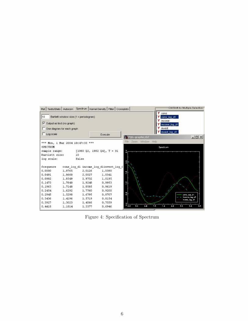
Figure 4: Specification of Spectrum

6

5 Crossplots

5.1 Background

Sometimes it is useful to investigate the direct relationship between two variables. Crossplots

offer an intuitive graphical tool to look at comovements between two different variables. It

may also be helpful to compare the plot with a simple OLS regression line, as well as with

a nonparametric estimate.

5.1.1 OLS Regression

Here a simple OLS regression is carried out, assuming that the model has the form

yt = α + βxt + ut, where ut is the regression error.

5.1.2 Nadaraya-Watson Regression

A possibly nonlinear regression function is assumed, m(x) = E(Y |X = x), x ∈ < with X

being the design variable and Y the response variable. The Nadaraya-Watson estimator is

defined as

m(x) =

∑Tt=1 ytK(x−xt

h)∑T

t=1 K(x−xt

h)

.

K is a kernel function. The kernels available in JMulTi are specified in Sec. 6. h is the

bandwidth. Here it is chosen automatically by

h = 0.9T−1/5 min(σx, IQR/1.34), see Silverman (1986), Eq. (3.31),

where σx is the standard deviation and IQR denotes the interquartile range of the xt obser-

vations. As usual, T is the sample size.

The nonparametric estimation does not assume a special functional form for the model and

can therefore capture possible nonlinearities in the relationship between X and Y .


5.2.1 Input

variables First select the variables that should be plotted against each other in the time

series list. They will appear in the two tables for the x- and y-axis. Then one can click on

a variable for each axis and invoke the plot.

7

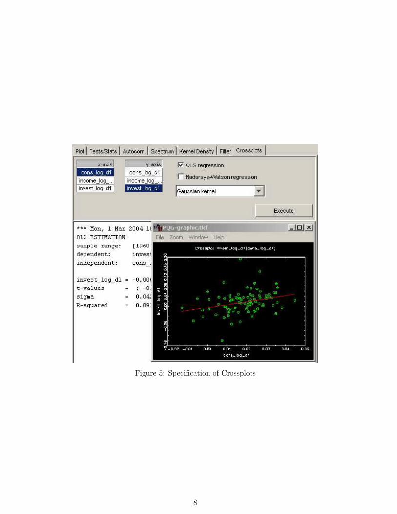
Figure 5: Specification of Crossplots

8

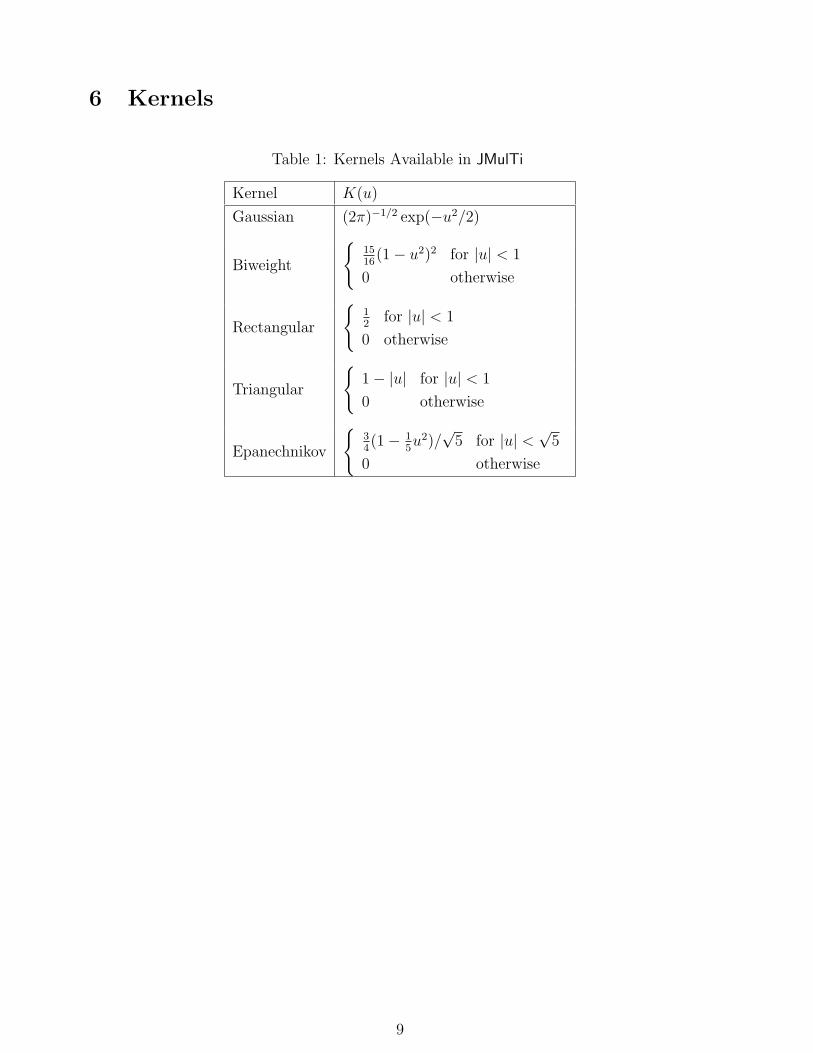
6 Kernels

Table 1: Kernels Available in JMulTi

Kernel K(u)

Gaussian (2π)−1/2 exp(−u2/2)

Biweight

{1516

(1− u2)2 for |u| < 1

0 otherwise

Rectangular

{12

for |u| < 1

0 otherwise

Triangular

{1− |u| for |u| < 1

0 otherwise

Epanechnikov

{34(1− 1

5u2)/

√5 for |u| < √

5

0 otherwise

9

7 Unit Root Tests

Because the order of integration of a time series is of great importance for the analysis, a

number of statistical tests have been developed for investigating it. In JMulTi there are

several tests implemented testing the null hypothesis that there is a unit root against the

alternative of stationarity of a DGP which may have a nonzero mean term, a deterministic

linear trend and perhaps seasonal dummy variables. The stochastic part is modeled by an

AR process or, alternatively, it is accounted for by nonparametric techniques. Another test

allows for the possibility of modeling structural shifts as they are observed. The KPSS test

checks the null hypothesis of stationarity against an alternative of a unit root.

10

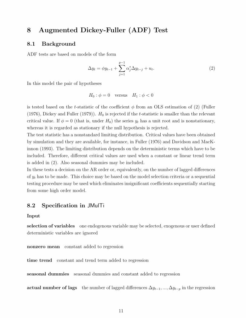
8 Augmented Dickey-Fuller (ADF) Test

8.1 Background

ADF tests are based on models of the form

∆yt = φyt−1 +

p−1∑j=1

α∗j∆yt−j + ut. (2)

In this model the pair of hypotheses

H0 : φ = 0 versus H1 : φ < 0

is tested based on the t-statistic of the coefficient φ from an OLS estimation of (2) (Fuller

(1976), Dickey and Fuller (1979)). H0 is rejected if the t-statistic is smaller than the relevant

critical value. If φ = 0 (that is, under H0) the series yt has a unit root and is nonstationary,

whereas it is regarded as stationary if the null hypothesis is rejected.

The test statistic has a nonstandard limiting distribution. Critical values have been obtained

by simulation and they are available, for instance, in Fuller (1976) and Davidson and MacK-

innon (1993). The limiting distribution depends on the deterministic terms which have to be

included. Therefore, different critical values are used when a constant or linear trend term

is added in (2). Also seasonal dummies may be included.

In these tests a decision on the AR order or, equivalently, on the number of lagged differences

of yt has to be made. This choice may be based on the model selection criteria or a sequential

testing procedure may be used which eliminates insignificant coefficients sequentially starting

from some high order model.


Input

selection of variables one endogenous variable may be selected, exogenous or user defined

deterministic variables are ignored

nonzero mean constant added to regression

time trend constant and trend term added to regression

seasonal dummies seasonal dummies and constant added to regression

actual number of lags the number of lagged differences ∆yt−1, ..., ∆yt−p in the regression

11

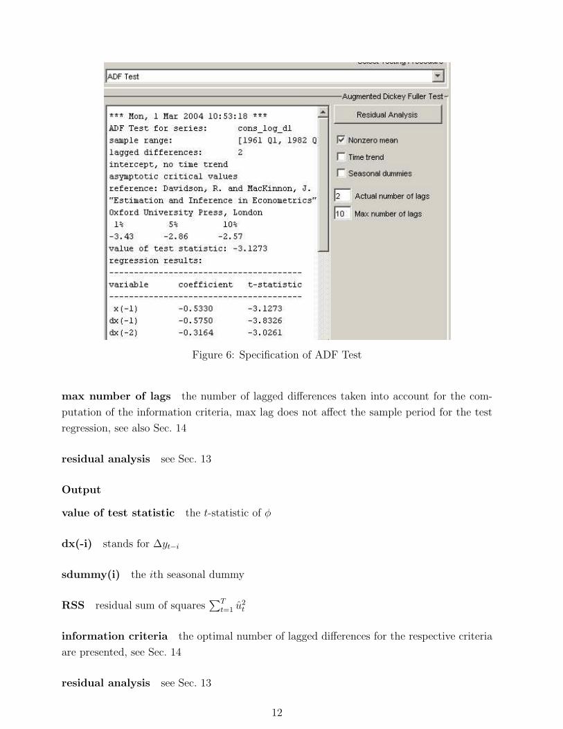
Figure 6: Specification of ADF Test

max number of lags the number of lagged differences taken into account for the com-

putation of the information criteria, max lag does not affect the sample period for the test

regression, see also Sec. 14

residual analysis see Sec. 13

Output

value of test statistic the t-statistic of φ

dx(-i) stands for ∆yt−i

sdummy(i) the ith seasonal dummy

RSS residual sum of squares∑T

t=1 u2t

information criteria the optimal number of lagged differences for the respective criteria

are presented, see Sec. 14


12

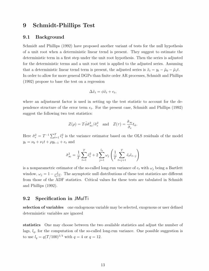
9 Schmidt-Phillips Test

9.1 Background

Schmidt and Phillips (1992) have proposed another variant of tests for the null hypothesis

of a unit root when a deterministic linear trend is present. They suggest to estimate the

deterministic term in a first step under the unit root hypothesis. Then the series is adjusted

for the deterministic terms and a unit root test is applied to the adjusted series. Assuming

that a deterministic linear trend term is present, the adjusted series is xt = yt − µ0 − µ1t.

In order to allow for more general DGPs than finite order AR processes, Schmidt and Phillips

(1992) propose to base the test on a regression

∆xt = φxt + et,

where an adjustment factor is used in setting up the test statistic to account for the de-

pendence structure of the error term et. For the present case, Schmidt and Phillips (1992)

suggest the following two test statistics:

Z(ρ) = T φσ2∞/σ2

e and Z(τ) =σ∞σe

tα.

Here σ2e = T−1

∑Tt=1 e2

t is the variance estimator based on the OLS residuals of the model

yt = ν0 + ν1t + ρyt−1 + et and

σ2∞ =

1

T

T∑t=1

e2t + 2

lq∑j=1

ωj

(1

T

T∑t=j+1

etet−j

)

is a nonparametric estimator of the so-called long-run variance of et with ωj being a Bartlett

window, ωj = 1− jlq+1

. The asymptotic null distributions of these test statistics are different

from those of the ADF statistics. Critical values for these tests are tabulated in Schmidt

and Phillips (1992).




statistics One may choose between the two available statistics and adjust the number of

lags, lq, for the computation of the so-called long-run variance. One possible suggestion is

to use lq = q(T/100)1/4 with q = 4 or q = 12.

13

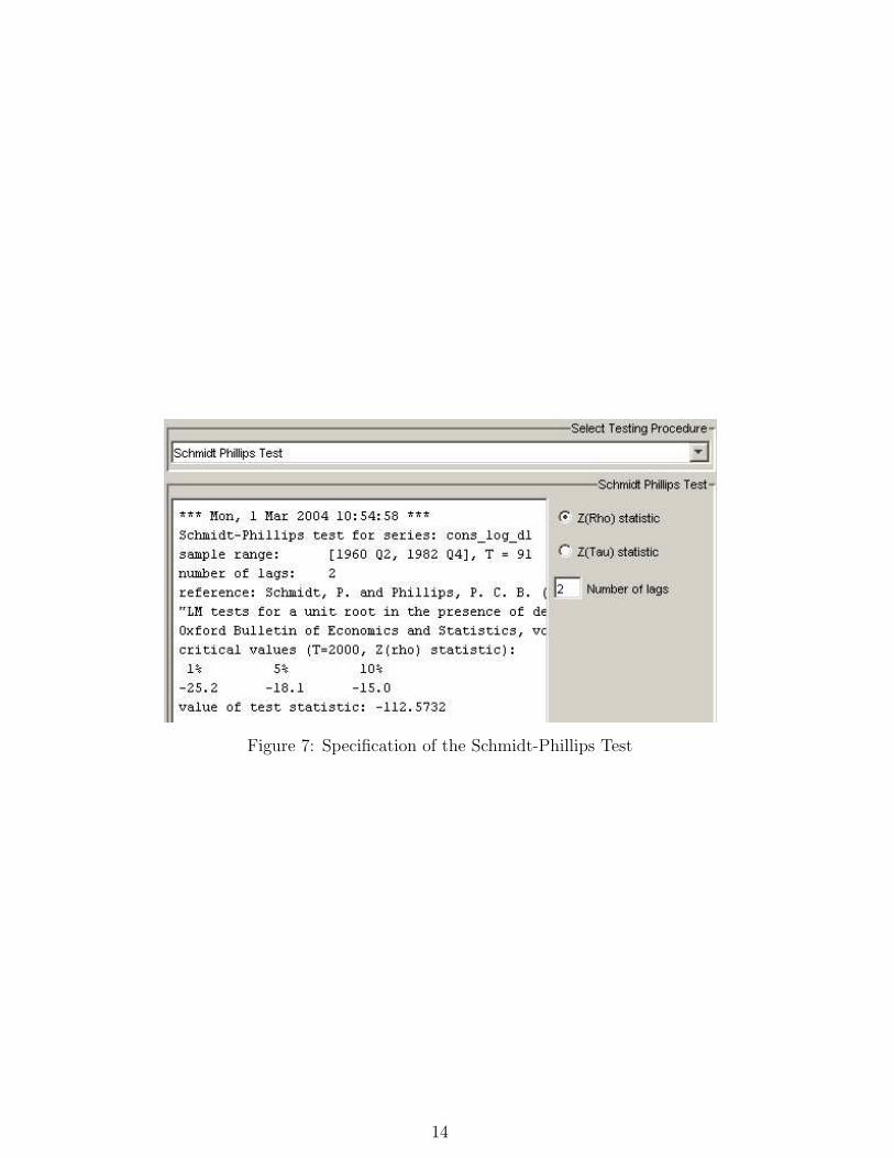
Figure 7: Specification of the Schmidt-Phillips Test

14

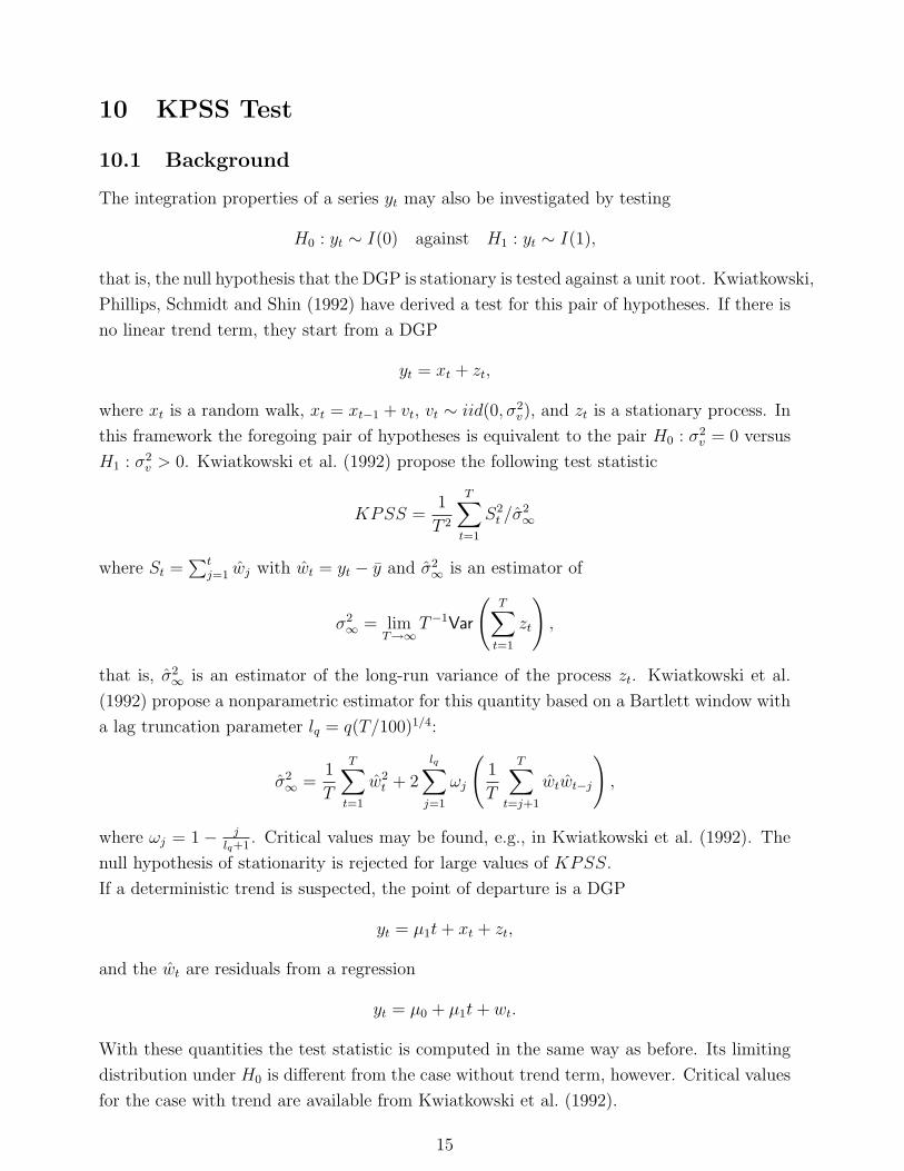
10 KPSS Test

10.1 Background

The integration properties of a series yt may also be investigated by testing

H0 : yt ∼ I(0) against H1 : yt ∼ I(1),

that is, the null hypothesis that the DGP is stationary is tested against a unit root. Kwiatkowski,

Phillips, Schmidt and Shin (1992) have derived a test for this pair of hypotheses. If there is

no linear trend term, they start from a DGP

yt = xt + zt,

where xt is a random walk, xt = xt−1 + vt, vt ∼ iid(0, σ2v), and zt is a stationary process. In

this framework the foregoing pair of hypotheses is equivalent to the pair H0 : σ2v = 0 versus

H1 : σ2v > 0. Kwiatkowski et al. (1992) propose the following test statistic

KPSS =1

T 2

T∑t=1

S2t /σ

2∞

where St =∑t

j=1 wj with wt = yt − y and σ2∞ is an estimator of

σ2∞ = lim

T→∞T−1Var

(T∑

t=1

zt

),

that is, σ2∞ is an estimator of the long-run variance of the process zt. Kwiatkowski et al.

(1992) propose a nonparametric estimator for this quantity based on a Bartlett window with

a lag truncation parameter lq = q(T/100)1/4:

σ2∞ =

1

T

T∑t=1

w2t + 2

lq∑j=1

ωj

(1

T

T∑t=j+1

wtwt−j

),

where ωj = 1 − jlq+1

. Critical values may be found, e.g., in Kwiatkowski et al. (1992). The

null hypothesis of stationarity is rejected for large values of KPSS.

If a deterministic trend is suspected, the point of departure is a DGP

yt = µ1t + xt + zt,

and the wt are residuals from a regression

yt = µ0 + µ1t + wt.

With these quantities the test statistic is computed in the same way as before. Its limiting

distribution under H0 is different from the case without trend term, however. Critical values

for the case with trend are available from Kwiatkowski et al. (1992).

15

Figure 8: Specification of the KPSS Test




statistics One may choose between the two possible statistics and adjust the number of

lags for the computation of the so-called long-run variance. Suitable choices of the lag length

lq may be l4 ≈ 4(T/100)1/4 or l12 ≈ 12(T/100)1/4.

16

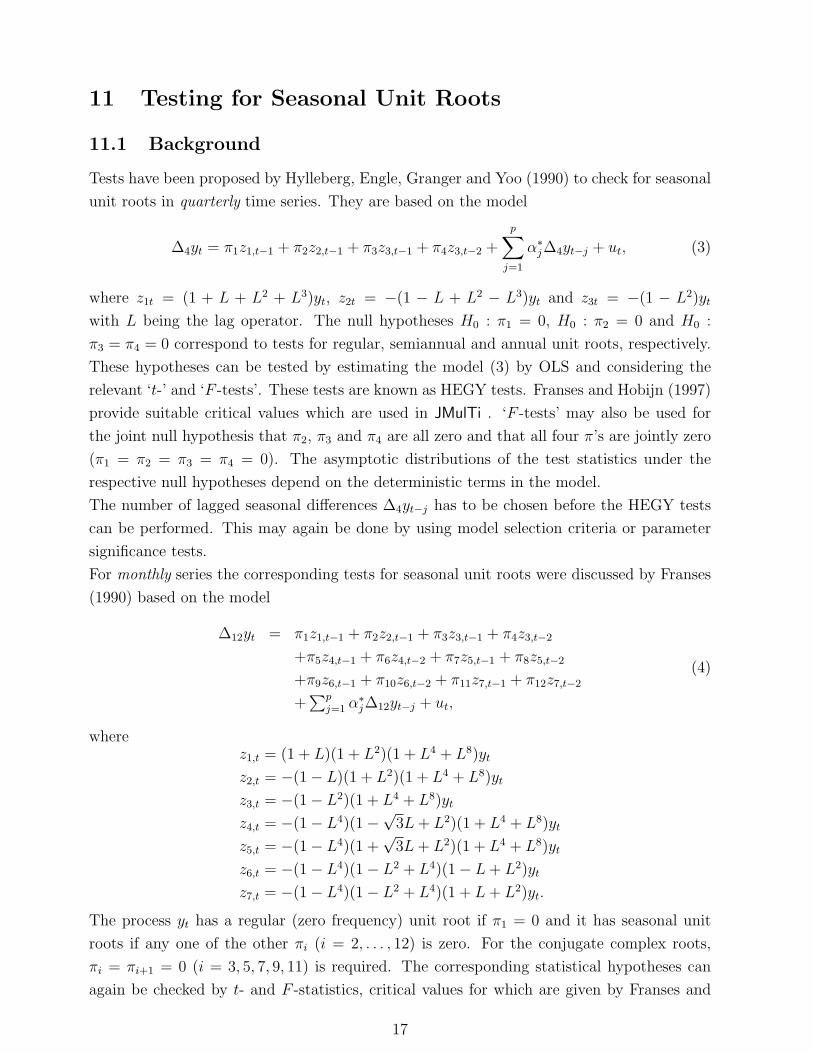
11 Testing for Seasonal Unit Roots

11.1 Background

Tests have been proposed by Hylleberg, Engle, Granger and Yoo (1990) to check for seasonal

unit roots in quarterly time series. They are based on the model

∆4yt = π1z1,t−1 + π2z2,t−1 + π3z3,t−1 + π4z3,t−2 +

p∑j=1

α∗j∆4yt−j + ut, (3)

where z1t = (1 + L + L2 + L3)yt, z2t = −(1 − L + L2 − L3)yt and z3t = −(1 − L2)yt

with L being the lag operator. The null hypotheses H0 : π1 = 0, H0 : π2 = 0 and H0 :

π3 = π4 = 0 correspond to tests for regular, semiannual and annual unit roots, respectively.

These hypotheses can be tested by estimating the model (3) by OLS and considering the

relevant ‘t-’ and ‘F -tests’. These tests are known as HEGY tests. Franses and Hobijn (1997)

provide suitable critical values which are used in JMulTi . ‘F -tests’ may also be used for

the joint null hypothesis that π2, π3 and π4 are all zero and that all four π’s are jointly zero

(π1 = π2 = π3 = π4 = 0). The asymptotic distributions of the test statistics under the

respective null hypotheses depend on the deterministic terms in the model.

The number of lagged seasonal differences ∆4yt−j has to be chosen before the HEGY tests

can be performed. This may again be done by using model selection criteria or parameter

significance tests.

For monthly series the corresponding tests for seasonal unit roots were discussed by Franses

(1990) based on the model

∆12yt = π1z1,t−1 + π2z2,t−1 + π3z3,t−1 + π4z3,t−2

+π5z4,t−1 + π6z4,t−2 + π7z5,t−1 + π8z5,t−2

+π9z6,t−1 + π10z6,t−2 + π11z7,t−1 + π12z7,t−2

+∑p

j=1 α∗j∆12yt−j + ut,

(4)

wherez1,t = (1 + L)(1 + L2)(1 + L4 + L8)yt

z2,t = −(1− L)(1 + L2)(1 + L4 + L8)yt

z3,t = −(1− L2)(1 + L4 + L8)yt

z4,t = −(1− L4)(1−√3L + L2)(1 + L4 + L8)yt

z5,t = −(1− L4)(1 +√

3L + L2)(1 + L4 + L8)yt

z6,t = −(1− L4)(1− L2 + L4)(1− L + L2)yt

z7,t = −(1− L4)(1− L2 + L4)(1 + L + L2)yt.

The process yt has a regular (zero frequency) unit root if π1 = 0 and it has seasonal unit

roots if any one of the other πi (i = 2, . . . , 12) is zero. For the conjugate complex roots,

πi = πi+1 = 0 (i = 3, 5, 7, 9, 11) is required. The corresponding statistical hypotheses can

again be checked by t- and F -statistics, critical values for which are given by Franses and

17

Hobijn (1997). If all the πi (i = 1, . . . , 12) are zero, then a stationary model for the monthly

seasonal differences of the series is suitable. As in the case of quarterly series it is also

possible to include deterministic terms in the model (4).


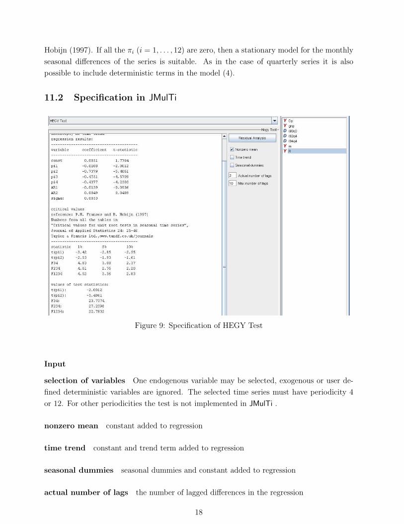
Figure 9: Specification of HEGY Test

Input

selection of variables One endogenous variable may be selected, exogenous or user de-

fined deterministic variables are ignored. The selected time series must have periodicity 4

or 12. For other periodicities the test is not implemented in JMulTi .

nonzero mean constant added to regression



actual number of lags the number of lagged differences in the regression

18

max number of lags the number of lagged differences taken into account for the compu-

tation of the information criteria, max lag does not affect the sample for the test regression,

see also Sec. 14


Output

pi 1,...,periodicity the results from the test regression (3) or (4)

AR 1,...,lags the coefficients of ∆4yt−i (∆12yt−i)

sdummy(i) the ith seasonal dummy

sigma the standard deviation√

u′u/(T −K), with K being the number of regressors

test statistics the respective F - and t-statistics along with the critical values, the pi(= π)

coefficients tested are indicated with an index:

• F1112 tests H0 : pi11=pi12=0

• F2-12 tests H0 : pi2=pi3=...=pi12=0

• t(pi1) tests H0 : pi1=0 , etc.

information criteria the optimal number of lagged differences found by the respective

criterion are presented, see Sec. 14


19

12 Tests for Processes with Level Shifts

12.1 Background

If there is a shift in the level of the DGP, it should be taken into account in testing for a

unit root because the ADF test may be distorted if the shift is simply ignored. Therefore a

shift function, which is here denoted by ft(θ)′γ, may be added to the deterministic term µt

of the DGP. Hence, a model

yt = µ0 + µ1t + ft(θ)′γ + xt, (5)

is considered, where θ and γ are unknown parameters or parameter vectors and the errors

xt are generated by an AR(p) process with possible unit root.

JMulTi offers the following three possible shift functions:

1. A simple shift dummy variable with shift date TB,

f(1)t = d1t :=

{0, t < TB

1, t ≥ TB

.

The function does not involve any extra parameter θ. In the shift term f(1)t γ, the

parameter γ is a scalar. Differencing this shift function leads to an impulse dummy.

2. The second shift function is based on the exponential distribution function which allows

for a nonlinear gradual shift to a new level starting at time TB,

f(2)t (θ) =

{0, t < TB

1− exp{−θ(t− TB + 1)}, t ≥ TB

.

In the shift term f(2)t (θ)γ, both θ and γ are scalar parameters. The first one is confined

to the positive real line (θ > 0), whereas the second one may assume any value.

3. The third function can be viewed as a rational function in the lag operator applied to

a shift dummy d1t,

f(3)t (θ) =

[d1,t

1− θL:

d1,t−1

1− θL

]′.

Here the actual shift term is [γ1(1 − θL)−1 + γ2(1 − θL)−1L]d1t, where θ is a scalar

parameter between 0 and 1 and γ = (γ1 : γ2)′ is a two-dimensional parameter vector.

Both f(2)t (θ)γ and f

(3)t (θ)′γ can generate sharp one-time shifts at time TB for suitable values

of θ. Thus they are more general than f(1)t γ.

Saikkonen and Lutkepohl (2002) and Lanne, Lutkepohl and Saikkonen (2002) propose unit

root tests for the model (5) which are based on estimating the deterministic term first

by a generalized least squares (GLS) procedure under the unit root null hypothesis and

20

subtracting it from the original series. Then an ADF type test is performed on the adjusted

series which also includes terms to correct for estimation errors in the parameters of the

deterministic part. As in the case of the ADF statistic, the asymptotic null distribution is

nonstandard. Critical values are tabulated in Lanne et al. (2002). Seasonal dummies may

be included in addition to a constant or a linear trend term.

The user of the test has to decide on the AR order and the shift date TB. If the latter quantity

is known, the desired shift function may be included and the AR order may be chosen in the

usual way with the help of order selection criteria, sequential tests and model checking tools.

If the break date is unknown, Lanne, Lutkepohl and Saikkonen (2001) recommend to choose

a reasonably large AR order in a first step and then pick the break date which minimizes the

GLS objective function used to estimate the parameters of the deterministic part. In this

step, JMulTi uses a shift dummy as shift function. The program offers graphs which show

the impact of changes in the break date and variations in the parameter θ. Once a possible

break date is fixed, a more detailed analysis of the AR order may be useful to improve the

power of the test.


Figure 10: UR Test with Level Shift

21

Figure 11: automatic break search

Input

selection of variables one endogenous variable may be selected, exogenous or user de-

fined deterministic variables are ignored, a constant is always automatically added to the

regression.

shift function select the desired shift function, an impulse dummy can be used with 1st

differences, for the exponential and rational shift function, the parameter theta(= θ) is

estimated by a grid search

break date the desired break date to be used in the regression, click on search to use an

automatic procedure to find the optimal break date



actual number of lags the number of lagged differences in the regression

22

max number of lags the number of lagged differences taken into account for the com-

putation of the information criteria, max lag does not affect the sample period for the test

regression, see also Sec. 14


graphical analysis shows plots of the shift function, the original series with and without

deterministic terms and the grid search for theta

Output

value of test statistic the t-statistic of the relevant parameter in the ADF type model

setup proposed by Lanne et al. (2002)

theta in case of exponential or rational shift function the estimated slope parameter

dx(-i) stands for ∆yt−i

d(const) stands for Z1 = [1, 0, . . . , 0]′, regressor for initial estimation of the constant

d(trend) stands for Z2 = [1, 1, . . . , 1]′, regressor for initial estimation of the trend

d(shiftfkt) stands for Z3 = [f1(θ) : ∆f2(θ) : · · · : ∆fT (θ)]′, regressor for initial estimation

of the shift parameter γ

d(SD) stands for the seasonal dummies which are included in the same way as Zi

RSS residual sum of squares∑T

t=1 u2t

information criteria the optimal number of lagged differences for the respective criteria

are presented, see Sec. 14


23

13 Residual Analysis


Figure 12: Specification of Residual Analysis

The configuration panel allows to specify a range of diagnostic tests for the residual analysis of

the estimated model. Select the appropriate checkboxes and adjust the available parameters

according to your needs. The residual analysis is then carried out after the respective model

is estimated.

13.2 Background

In the following the residual series are denoted by ut (t = 1, . . . , T ) and the standardized

residuals are obtained by dividing by the standard deviation, that is, the standardized resid-

uals are ust = (ut − ¯u)/σu, where σ2

u = T−1∑T

t=1(ut − ¯u)2 with ¯u = T−1∑T

t=1 ut.

Portmanteau Test

The pair of hypotheses

H0 : ρu,1 = · · · = ρu,h = 0 vs. H1 : ρu,i 6= 0 for at least one i = 1, . . . , h,

is tested. Here ρu,i = Corr(ut, ut−i) denotes the AC coefficients of the residual series. Two

test statistics, Qh and LBh, are given in JMulTi together with the corresponding p-values

24

(see Ljung and Box (1978)):

Qh = T

h∑j=1

ρ2u,j and LBh = T 2

h∑j=1

1

T − jρ2

u,j

where ρu,j = T−1∑T

t=j+1 ust u

st−j. If the ut are residuals from an estimated ARMA(p, q)

model, the test statistics have an approximate asymptotic χ2(h − p − q) distribution if the

null hypothesis holds.

ARCH-LM Test

In JMulTi the test for neglected conditional heteroskedasticity (ARCH) is based on fitting

an ARCH(q) model to the estimation residuals,

u2t = β0 + β1u

2t−1 + · · ·+ βqu

2t−q + errort, (6)

and checking the null hypothesis

H0 : β1 = · · · = βq = 0 vs. H1 : β1 6= 0 or . . . or βq 6= 0.

Under normality assumptions the LM test statistic is obtained from the coefficient of deter-

mination, R2, of the regression (6):

ARCHLM(q) = TR2.

It has an asymptotic χ2(q) distribution if the null hypothesis of no conditional heteroskedas-

ticity holds (Engle (1982)).

Jarque-Bera Test

Lomnicki (1961) and Jarque and Bera (1987) have proposed a test for nonnormality based

on the skewness and kurtosis of a distribution. The test checks the pair of hypotheses

H0 : E(ust)

3 = 0 and E(ust)

4 = 3 vs. H1 : E(ust)

3 6= 0 or E(ust)

4 6= 3.

The test statistic is

JB =T

6

[T−1

T∑t=1

(ust)

3

]2

+T

24

[T−1

T∑t=1

(ust)

4 − 3

]2

,

and has an asymptotic χ2(2) distribution if the null hypothesis is correct (see Jarque and

Bera (1987)). In JMulTi also skewness and kurtosis of the standardized residuals are given.

Plot Residuals

Absolute or standardized residuals are plotted.

25

Plot Autocorrelation

In JMulTi residual autocorrelations (ACs) ρu,h = γu,h/γu,0 are obtained from

γh =1

T

T∑

t=h+1

(ut − ¯u)(ut−h − ¯u)

where ¯u = T−1∑T

t=1 ut is the sample mean.

The partial autocorrelation (PAC) between ut and ut−h is the conditional autocorrelation

given ut−1, . . . , ut−h+1. The corresponding sample quantity ah is obtained as the OLS esti-

mator of the coefficient αh in an autoregressive model

ut = ν + α1ut−1 + · · ·+ αhut−h + errort.

In JMulTi , OLS estimates are obtained for each h with sample size T − h.

26

14 Information Criteria

The following formulas for the information criteria are used:

AIC(n) = log σ2u(n) +

2

Tn (Akaike (1973, 1974)) ,

HQ(n) = log σ2u(n) +

2 log log T

Tn (Hannan and Quinn (1979)),

SC(n) = log σ2u(n) +

log T

Tn (Schwarz (1978) and Rissanen (1978)),

and

FPE(n) =T + n∗

T − n∗σ2

u(n) (Akaike (1969)),

where σ2u(n) is estimated by u′u/T , n is the number of lagged differences included and n∗ is

the total number of parameters in the model when n lagged differences are included.

The computation of the ut is always done with a regression model that is estimated with OLS.

All models with 0 to n lagged differences are estimated. The lag length which minimizes the

respective information criterion is presented. The sample length is the same for all different

lag lengths and is determined by the maximum order. In other words, the number of values

set aside as presample values is determined by the maximum lag order.

27

15 Cointegration Tests

The cointegration tests in JMulTi are based on the following general model

yt = Dt + xt

where yt is a K-dimensional vector of observable variables, Dt is a deterministic term, e.g.,

Dt = µ0 + µ1t may be a linear trend term, and xt is a VAR(p) process with vector error

correction model (VECM) representation

∆xt = Πxt−1 +

p−1∑j=1

Γj∆yt−j + ut

Here ut is a vector white noise process with ut ∼ (0, Σu). The rank of Π is the cointegrating

rank of xt and hence of yt. Therefore the cointegration tests check the pair of hypotheses

H0(r0) : rk(Π) = r0 versus H1(r0) : rk(Π) > r0, r0 = 0, . . . , K − 1 (7)

Two types of tests are available in JMulTi , Johansen trace tests and tests proposed by

Saikkonen & Lutkepohl. For both types of tests the VAR order p has to be specified. Model

selection criteria offer help in the decision on the VAR order (see Sec. 18).

28

16 Johansen Trace Tests

16.1 Background

Johansen (1988, 1991, 1992, 1994, 1995) in a series of publications has proposed tests

which are likelihood ratio (LR) tests if yt is normally distributed and Gaussian pseudo LR

tests otherwise. In the literature these tests are known as trace tests because of the special

form of the test statistic. The distributions of the test statistics under their respective null

hypotheses depend on the deterministic terms. In JMulTi three basic modelling options are

available where in each case seasonal dummy variables and impulse dummies may be added.

Furthermore, in case 1 and 2 the user may specify up to two structural breaks which appear

either in levels only or in trend and levels jointly (only case 2).

Eviews Compatibility Guide

Users with experience in the econometric software package Eviews should note that in JMulTi

only three relevant test cases are implemented, which are described in the following sections.

The mapping between the Eviews and JMulTi model specification options is the following

(Eviews - JMulTi):

• no intercept in CE or VAR - not implemented

• intercept in CE, no intercept in VAR - constant (case 1)

• intercept in CE and test VAR - orthogonal trend (case 3)

• intercept and trend in CE, no trend in VAR - constant and trend (case 2)

• intercept and trend in CE, linear trend in VAR - not implemented

Case 1: Restricted mean term and no linear trend

In this case the deterministic term has the form

Dt = µ0(+seasonal dummies)

and the DGP of the yt can be written as

∆yt = Π∗[

yt−1

1

]+

p−1∑j=1

Γj∆yt−j + ut

where Π∗ = [Π : ν0] is (K × (K + 1)) with ν0 = −Πµ0 and the seasonals are neglected. The

test statistic is obtained by reduced rank regression applied to this model with rk(Π∗) = r0

(see Johansen (1995)).

29

Case 2: Constant and linear trend

In this case the deterministic term has the form

Dt = µ0 + µ1t(+seasonal dummies)

and the DGP of the yt can be written as

∆yt = ν + Π+

[yt−1

t− 1

]+

p−1∑j=1

Γj∆yt−j + ut

where Π+ = α[β′ : η] is a (K × (K + 1)) matrix of rank r0 with η = −β′µ1 and the seasonals

are neglected. The test is based on this model (see Johansen (1994, 1995)).

Case 3: Trend orthogonal to cointegration relations

In this case the deterministic term again has the form

Dt = µ0 + µ1t(+seasonal dummies)

It is assumed, however, that there is a linear trend term in the variables but not in the

cointegration relations (it is orthogonal to the cointegration relations) so that Π(yt−1−µ0−µ1(t− 1)) = Π(yt−1 − µ0). In this case the model for yt can be written as

∆yt = ν + Πyt−1 +

p−1∑j=1

Γj∆yt−j + ut

(see Johansen (1995)). In this setup it is not meaningful to test H0 : rk(Π) = K − 1 versus

H1 : rk(Π) = K, as argued by Saikkonen and Lutkepohl (2000a).


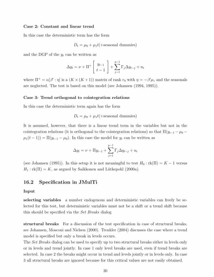
Input

selecting variables a number endogenous and deterministic variables can freely be se-

lected for this test, but deterministic variables must not be a shift or a trend shift because

this should be specified via the Set Breaks dialog

structural breaks For a discussion of the test specification in case of structural breaks,

see Johansen, Mosconi and Nielsen (2000). Trenkler (2004) discusses the case where a trend

model is specified but only a break in levels occurs.

The Set Breaks dialog can be used to specify up to two structural breaks either in levels only

or in levels and trend jointly. In case 1 only level breaks are used, even if trend breaks are

selected. In case 2 the breaks might occur in trend and levels jointly or in levels only. In case

3 all structural breaks are ignored because for this critical values are not easily obtained.

30

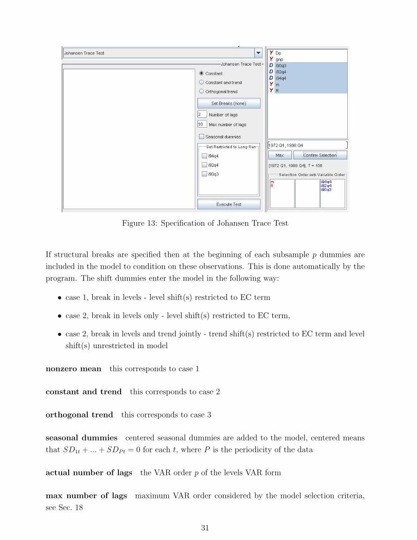
Figure 13: Specification of Johansen Trace Test

If structural breaks are specified then at the beginning of each subsample p dummies are

included in the model to condition on these observations. This is done automatically by the

program. The shift dummies enter the model in the following way:

• case 1, break in levels - level shift(s) restricted to EC term

• case 2, break in levels only - level shift(s) restricted to EC term,

• case 2, break in levels and trend jointly - trend shift(s) restricted to EC term and level

shift(s) unrestricted in model

nonzero mean this corresponds to case 1

constant and trend this corresponds to case 2

orthogonal trend this corresponds to case 3

seasonal dummies centered seasonal dummies are added to the model, centered means

that SD1t + ... + SDPt = 0 for each t, where P is the periodicity of the data

actual number of lags the VAR order p of the levels VAR form

max number of lags maximum VAR order considered by the model selection criteria,

see Sec. 18

31

Figure 14: Specification of Level and Trend Breaks

set restricted to long run If additional impulse dummies terms are included they appear

in a list. By selecting them one can create a model of the form

∆yt = Π

[yt−1

Dlt−1

]+

p−1∑j=1

Γj∆yt−j + ut

with Dlt being the vector of deterministic terms restricted to the EC term.

Output

r0 the tested rank of the matrix Π under H0, r0 = 0, ..., K − 1, in case of an orthogonal

trend r0 = 0, ..., K − 2, see Sec. 16.1

critical values and p-values The critical values as well as the p-values of all Johansen

trace tests are obtained by computing the respective response surface according to Doornik

(1998) if there are no breaks, or according to Johansen et al. (2000) if there are up to 2

breaks. In case 2 with a break only in the levels the response surface also follows the design

of Johansen et al. (2000). However, the simulation of the limiting distribution is based on a

representation as in Theorem 3.1 for the case of no trend breaks.

optimal number of lags the optimal VAR order determined by the information criteria

32

17 Saikkonen & Lutkepohl Tests

17.1 Background

Saikkonen and Lutkepohl (2000a, b,c) have proposed tests for the pair of hypotheses (7)

which proceed by estimating the deterministic term Dt first, subtracting it from the obser-

vations and applying a Johansen type test to the adjusted series. In other words, the test is

based on a reduced rank regression of the system

∆xt = Πxt−1 +

p−1∑j=1

Γj∆xt−j + ut

where xt = yt− Dt and Dt is the estimated deterministic term. The parameters of the deter-

ministic term are estimated by the GLS procedure proposed by Saikkonen and Lutkepohl.

The critical values depend on the kind of deterministic term included. Possible options are

a constant, a linear trend term, a linear trend orthogonal to the cointeration relations and

seasonal dummy variables. In other words, all the options available for the Johansen trace

tests are also available here. In addition, the critical values remain valid if a shift dummy

variable is included. However, trend breaks are ignored by this test.


Figure 15: Specification of S&L Test

33

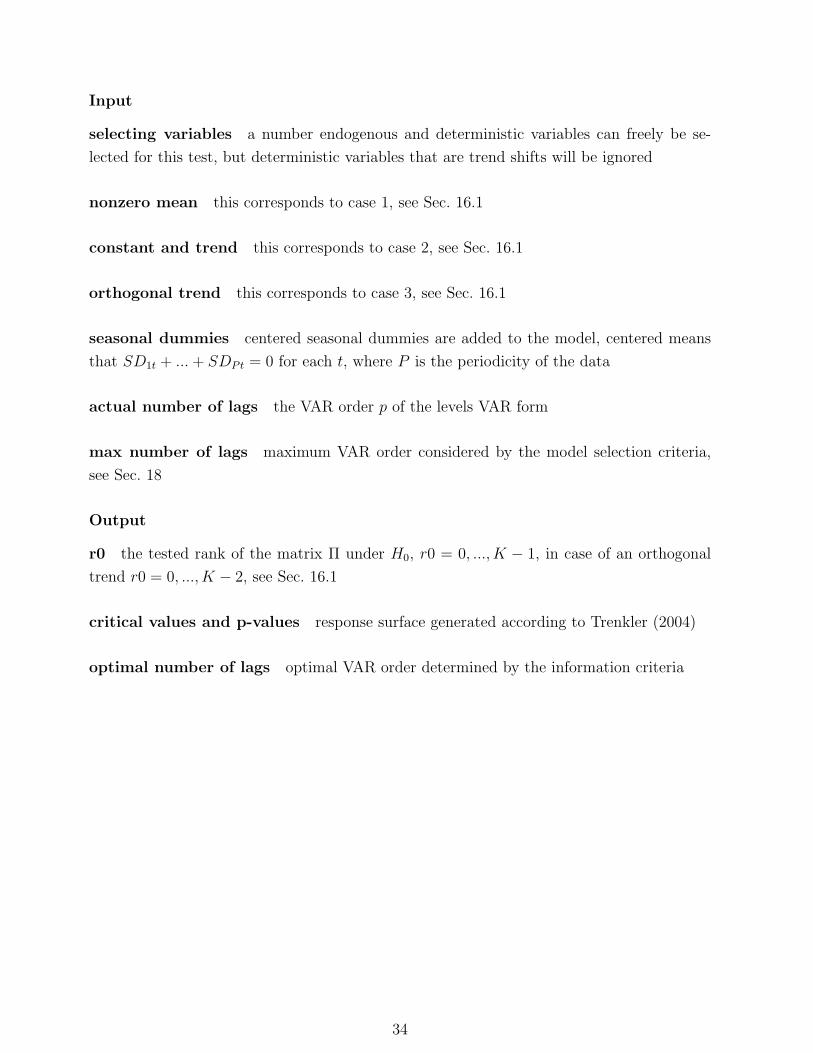
Input

selecting variables a number endogenous and deterministic variables can freely be se-

lected for this test, but deterministic variables that are trend shifts will be ignored

nonzero mean this corresponds to case 1, see Sec. 16.1

constant and trend this corresponds to case 2, see Sec. 16.1

orthogonal trend this corresponds to case 3, see Sec. 16.1

seasonal dummies centered seasonal dummies are added to the model, centered means

that SD1t + ... + SDPt = 0 for each t, where P is the periodicity of the data

actual number of lags the VAR order p of the levels VAR form

max number of lags maximum VAR order considered by the model selection criteria,

see Sec. 18

Output

r0 the tested rank of the matrix Π under H0, r0 = 0, ..., K − 1, in case of an orthogonal

trend r0 = 0, ..., K − 2, see Sec. 16.1

critical values and p-values response surface generated according to Trenkler (2004)

optimal number of lags optimal VAR order determined by the information criteria

34

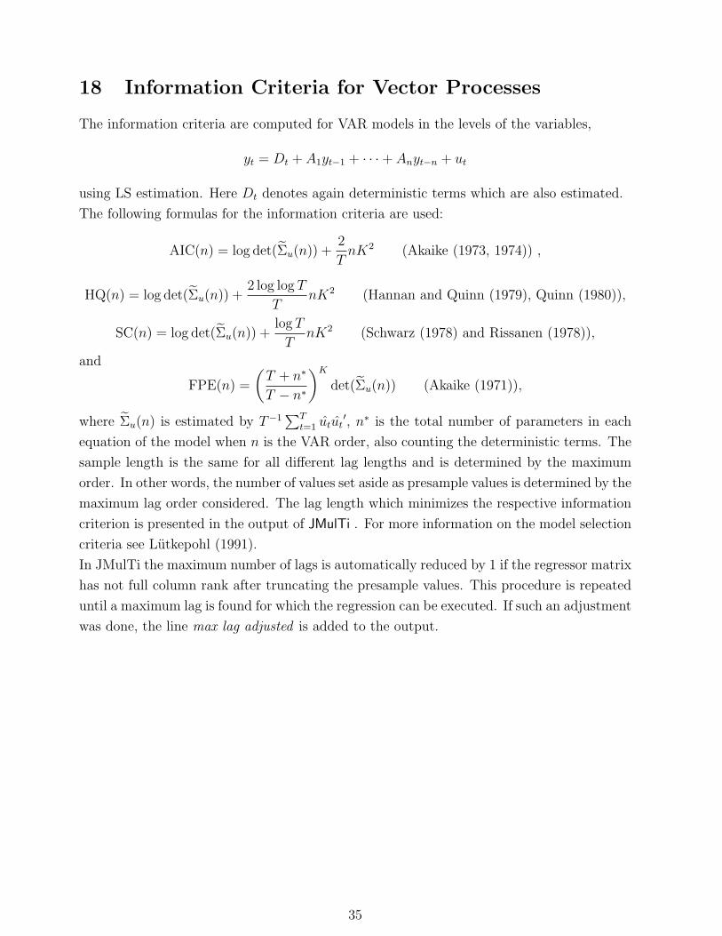
18 Information Criteria for Vector Processes

The information criteria are computed for VAR models in the levels of the variables,

yt = Dt + A1yt−1 + · · ·+ Anyt−n + ut

using LS estimation. Here Dt denotes again deterministic terms which are also estimated.

The following formulas for the information criteria are used:

AIC(n) = log det(Σu(n)) +2

TnK2 (Akaike (1973, 1974)) ,

HQ(n) = log det(Σu(n)) +2 log log T

TnK2 (Hannan and Quinn (1979), Quinn (1980)),

SC(n) = log det(Σu(n)) +log T

TnK2 (Schwarz (1978) and Rissanen (1978)),

and

FPE(n) =

(T + n∗

T − n∗

)K

det(Σu(n)) (Akaike (1971)),

where Σu(n) is estimated by T−1∑T

t=1 utut′, n∗ is the total number of parameters in each

equation of the model when n is the VAR order, also counting the deterministic terms. The

sample length is the same for all different lag lengths and is determined by the maximum

order. In other words, the number of values set aside as presample values is determined by the

maximum lag order considered. The lag length which minimizes the respective information

criterion is presented in the output of JMulTi . For more information on the model selection

criteria see Lutkepohl (1991).

In JMulTi the maximum number of lags is automatically reduced by 1 if the regressor matrix

has not full column rank after truncating the presample values. This procedure is repeated

until a maximum lag is found for which the regression can be executed. If such an adjustment

was done, the line max lag adjusted is added to the output.

35

References

Akaike, H. (1969). Fitting autoregressive models for prediction, Annals of the Institute of

Statistical Mathematics 21: 243–247.

Akaike, H. (1971). Autoregressive model fitting for control, Annals of the Institute of Sta-

tistical Mathematics 23: 163–180.

Akaike, H. (1973). Information theory and an extension of the maximum likelihood principle,

in B. Petrov and F. Csaki (eds), 2nd International Symposium on Information Theory,

Academiai Kiado, Budapest, pp. 267–281.

Akaike, H. (1974). A new look at the statistical model identification, IEEE Transactions on

Automatic Control AC-19: 716–723.

Bartlett, M. S. (1950). Periodogram analysis and continuous spectra, Biometrika 37: 1–16.

Davidson, R. and MacKinnon, J. (1993). Estimation and Inference in Econometrics, Oxford

University Press, London.

Dickey, D. A. and Fuller, W. A. (1979). Estimators for autoregressive time series with a unit

root, Journal of the American Statistical Association 74: 427–431.

Doornik, J. A. (1998). Approximations to the asymptotic distributions of cointegration tests,

Journal of Economic Surveys 12: 573–593.

Engle, R. F. (1982). Autoregressive conditional heteroscedasticity, with estimates of the

variance of United Kingdoms inflations, Econometrica 50: 987–1007.

Franses, P. H. (1990). Testing for seasonal unit roots in monthly data, Econometric Institute

Report 9032A, Erasmus University Rotterdam.

Franses, P. H. and Hobijn, B. (1997). Critical values for unit root tests in seasonal time

series, Journal of Applied Statistics 24: 25–46.

Fuller, W. A. (1976). Introduction to Statistical Time Series, John Wiley & Sons, New York.

Hannan, E. J. and Quinn, B. G. (1979). The determination of the order of an autoregression,

Journal of the Royal Statistical Society B41: 190–195.

Hylleberg, S., Engle, R. F., Granger, C. W. J. and Yoo, B. S. (1990). Seasonal integration

and cointegration, Journal of Econometrics 44: 215–238.

Jarque, C. M. and Bera, A. K. (1987). A test for normality of observations and regression

residuals, International Statistical Review 55: 163–172.

36

Johansen, S. (1988). Statistical analysis of cointegration vectors, Journal of Economic Dy-

namics and Control 12: 231–254.

Johansen, S. (1991). Estimation and hypothesis testing of cointegration vectors in Gaussian

vector autoregressive models, Econometrica 59: 1551–1581.

Johansen, S. (1992). Determination of cointegration rank in the presence of a linear trend,

Oxford Bulletin of Economics and Statistics 54: 383–397.

Johansen, S. (1994). The role of the constant and linear terms in cointegration analysis of

nonstationary time series, Econometric Reviews 13: 205–231.

Johansen, S. (1995). Likelihood-based Inference in Cointegrated Vector Autoregressive Models,

Oxford University Press, Oxford.

Johansen, S., Mosconi, R. and Nielsen, B. (2000). Cointegration analysis in the presence of

structural breaks in the deterministic trend, Econometrics Journal 3: 216–249.

Kwiatkowski, D., Phillips, P. C. B., Schmidt, P. and Shin, Y. (1992). Testing the null of

stationarity against the alternative of a unit root: How sure are we that the economic

time series have a unit root?, Journal of Econometrics 54: 159–178.

Lanne, M., Lutkepohl, H. and Saikkonen, P. (2001). Test procedures for unit roots in time

series with level shifts at unknown time, Discussion paper, Humboldt-Universitat Berlin.

Lanne, M., Lutkepohl, H. and Saikkonen, P. (2002). Comparison of unit root tests for time

series with level shifts, Journal of Time Series Analysis .

Ljung, G. M. and Box, G. E. P. (1978). On a measure of lack of fit in time-series models,

Biometrika 65: 297–303.

Lomnicki, Z. A. (1961). Tests for departure from normality in the case of linear stochastic

processes, Metrika 4: 37–62.

Lutkepohl, H. (1991). Introduction to Multiple Time Series Analysis, Springer Verlag, Berlin.

Quinn, B. G. (1980). Order determination for a multivariate autoregression, Journal of the

Royal Statistical Society B42: 182–185.

Rissanen, J. (1978). Modeling by shortest data description, Automatica 14: 465–471.

Saikkonen, P. and Lutkepohl, H. (2000a). Testing for the cointegrating rank of a VAR

process with an intercept, Econometric Theory 16: 373–406.

Saikkonen, P. and Lutkepohl, H. (2000b). Testing for the cointegrating rank of a VAR

process with structural shifts, Journal of Business & Economic Statistics 18: 451–464.

37

Saikkonen, P. and Lutkepohl, H. (2000c). Trend adjustment prior to testing for the cointe-

grating rank of a vector autoregressive process, Journal of Time Series Analysis 21: 435–

456.

Saikkonen, P. and Lutkepohl, H. (2002). Testing for a unit root in a time series with a level

shift at unknown time, Econometric Theory 18: 313–348.

Schmidt, P. and Phillips, P. C. B. (1992). LM tests for a unit root in the presence of

deterministic trends, Oxford Bulletin of Economics and Statistics 54: 257–287.

Schwarz, G. (1978). Estimating the dimension of a model, Annals of Statistics 6: 461–464.

Silverman, B. W. (1986). Density Estimation for Statistics and Data Analysis, Chapman &

Hall, London.

Trenkler, C. (2004). Determining p-values for systems cointegration tests with a prior ad-

justment for deterministic terms, mimeo, Humboldt-Universitat zu Berlin.

38

Initial Analysis in JMulTi · In this model the pair of hypotheses H0: φ = 0 versus H1: φ < 0 is...

Documents

Transcript of Initial Analysis in JMulTi · In this model the pair of hypotheses H0: φ = 0 versus H1: φ < 0 is...