Inferential Statistics & Test of Significance. Confidence Interval (CI) Y = mean Z = Z score related...
33
Inferential Statistics & Test of Significance
-
Upload
philip-sharp -
Category
Documents
-
view
218 -
download
0
Transcript of Inferential Statistics & Test of Significance. Confidence Interval (CI) Y = mean Z = Z score related...
Inferential Statistics & Test of Significance
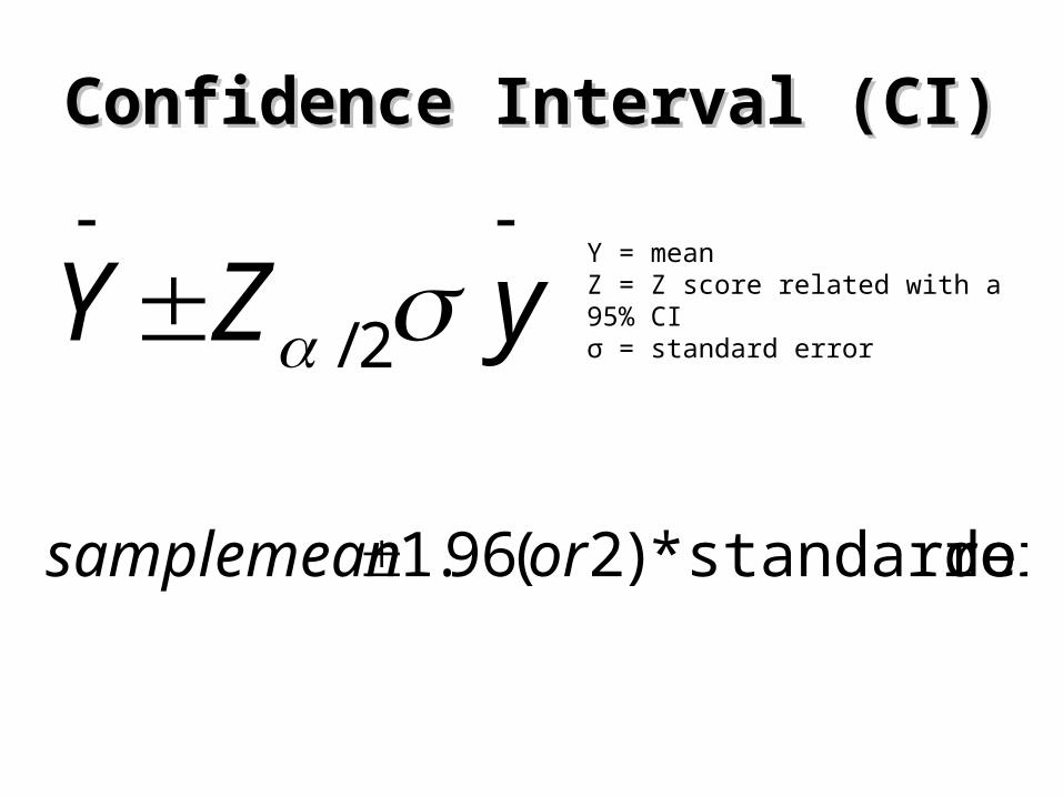
Confidence Interval (CI)Confidence Interval (CI)
yZY 2/
Y = mean Z = Z score related with a 95% CI σ = standard error
rorstandarder*)2(96.1 orsamplemean
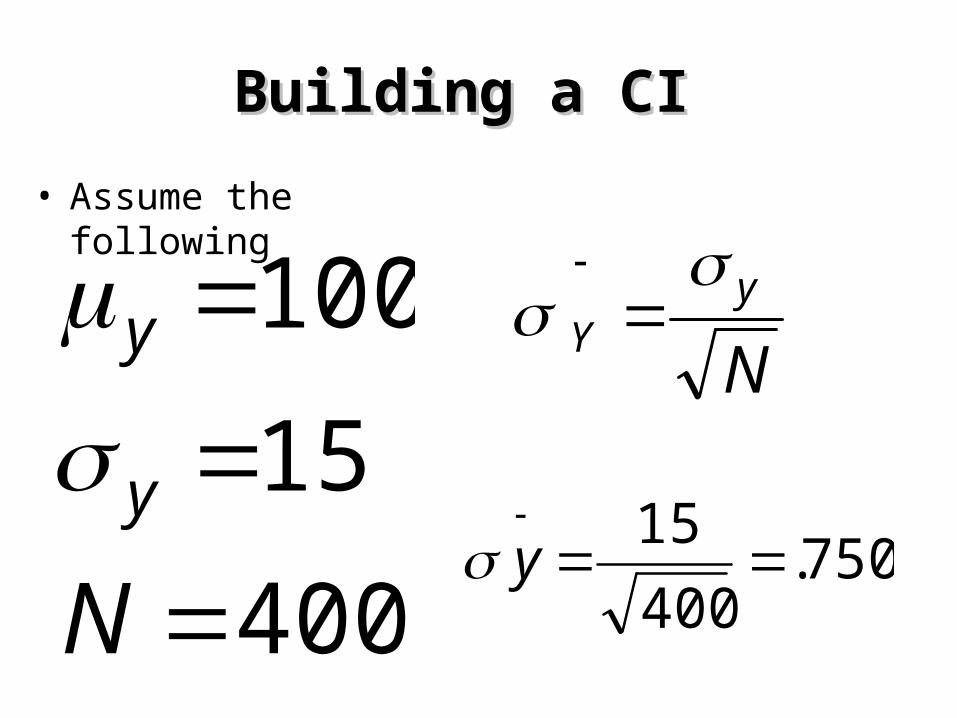
Building a CIBuilding a CI
N
yY
• Assume the following
400
15
100
N
y
y
750.400
15
y
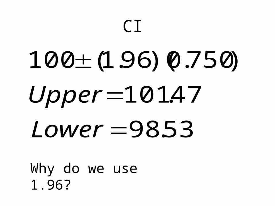
CI
53.98
47.101
)750.0)(96.1(100
Lower
Upper
Why do we use 1.96?
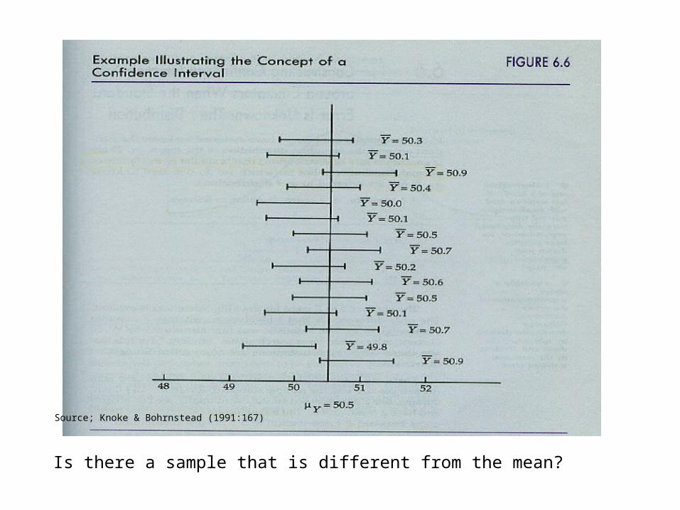
Is there a sample that is different from the mean?
Source; Knoke & Bohrnstead (1991:167)
Significance TestingSignificance Testing
• When we explain some phenomenon we move beyond description to inferential statistics and hypothesis testing.
• Tests of significance allow us to test hypotheses, and when we find a relationship between variables, reject the null hypothesis.
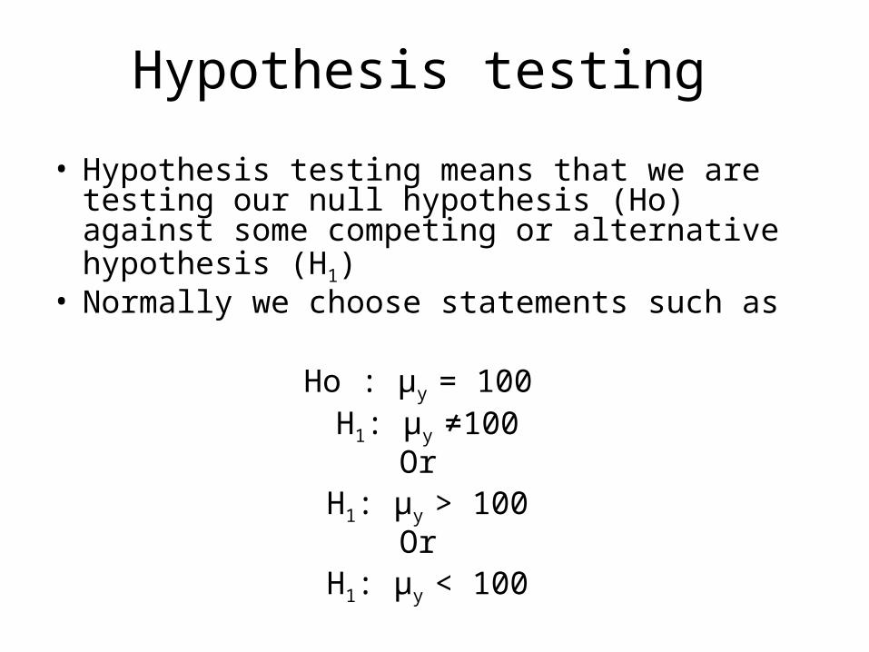
Hypothesis testing
• Hypothesis testing means that we are testing our null hypothesis (Ho) against some competing or alternative hypothesis (H1)
• Normally we choose statements such as
Ho : μy = 100 H1: μy ≠100
Or H1: μy > 100
Or H1: μy < 100

Significance TestingSignificance Testing• Even with high powered statistical measures,
there will be results that pop up that are affected by chance. If we were to keep running our models a thousand times, or fewer, we would likely see some results that do not stem from systematic processes.
• Thus, we need to determine at what level of significance we are willing to frame our results. We can never be 100% confident.
• Conventional levels of significance where we reject the null hypothesis are usually .05 or .01. The probability .10 is weakly significant.
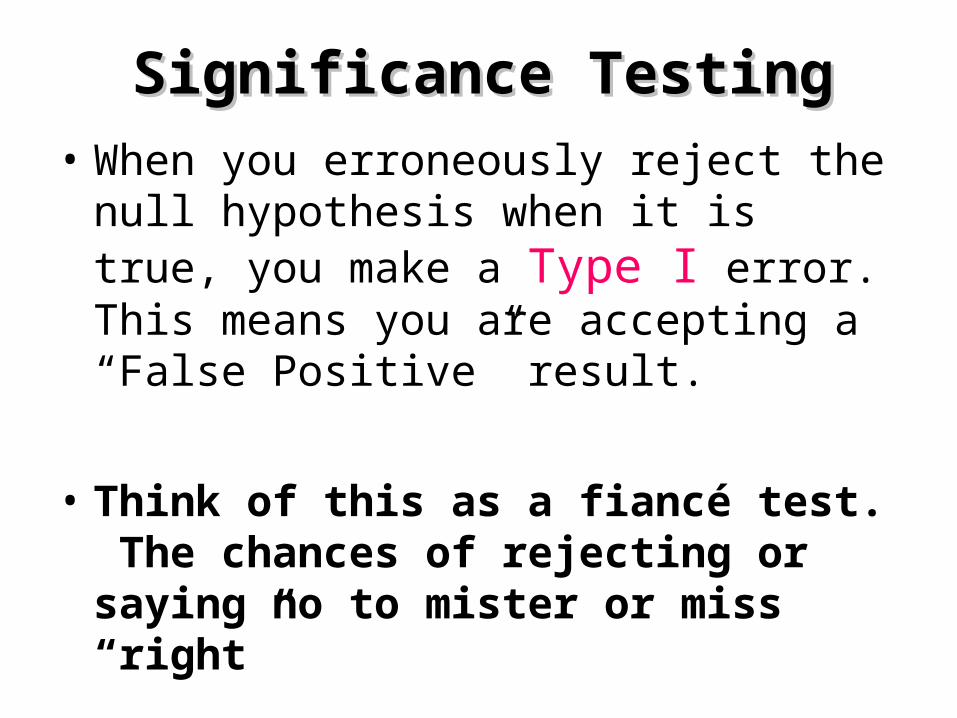
Significance TestingSignificance Testing• When you erroneously reject the null
hypothesis when it is true, you make a Type I error. This means you are accepting a “False Positive” result.
• Think of this as a fiancé test. The chances of rejecting or saying no to mister or miss “right”
SignificanceSignificance TestingTesting
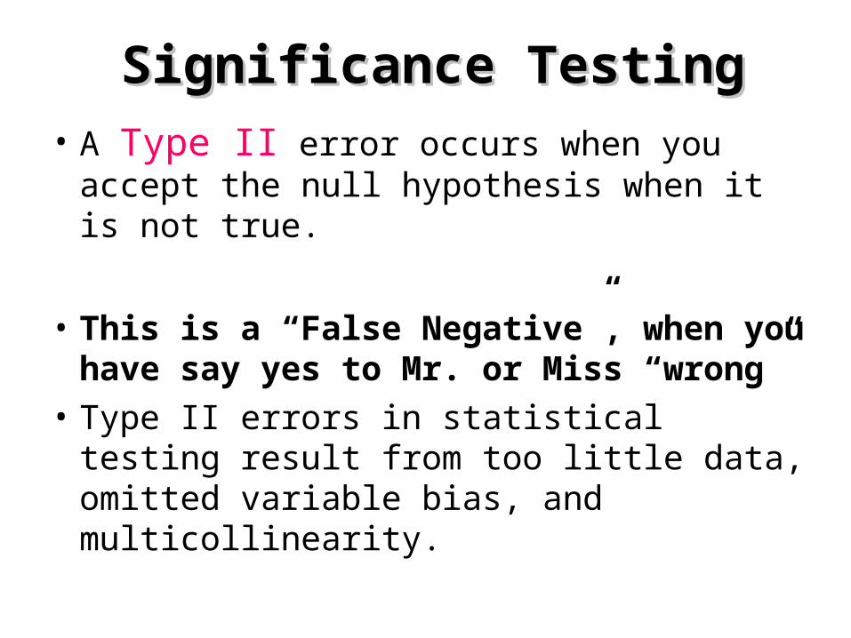
• A Type II error occurs when you accept the null hypothesis when it is not true.
• This is a “False Negative”, when you have say yes to Mr. or Miss “wrong”
• Type II errors in statistical testing result from too little data, omitted variable bias, and multicollinearity.
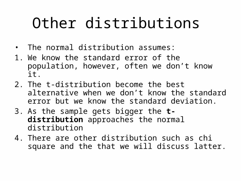
Other distributions
• The normal distribution assumes:1. We know the standard error of the population,
however, often we don’t know it. 2. The t-distribution become the best alternative
when we don’t know the standard error but we know the standard deviation.
3. As the sample gets bigger the t-distribution approaches the normal distribution
4. There are other distribution such as chi square and the that we will discuss latter.
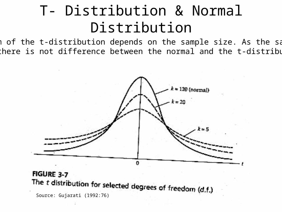
T- Distribution & Normal Distribution
Source: Gujarati (1992:76)
The form of the t-distribution depends on the sample size. As the sample getsLarger there is not difference between the normal and the t-distribution
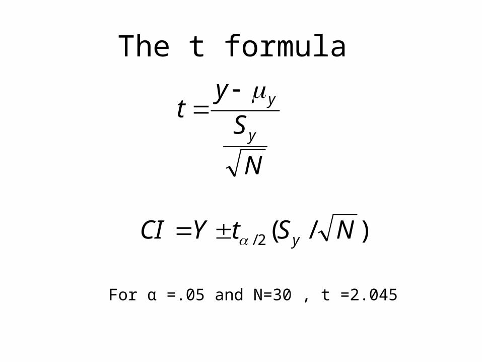
The t formula
N
S
yt
y
y
)/(2/ NStYCI y
For α =.05 and N=30 , t =2.045
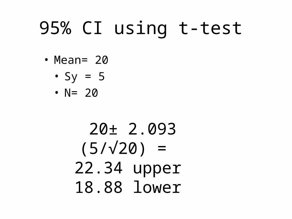
95% CI using t-test
• Mean= 20 • Sy = 5• N= 20
20± 2.093 (5/√20) = 22.34 upper 18.88 lower
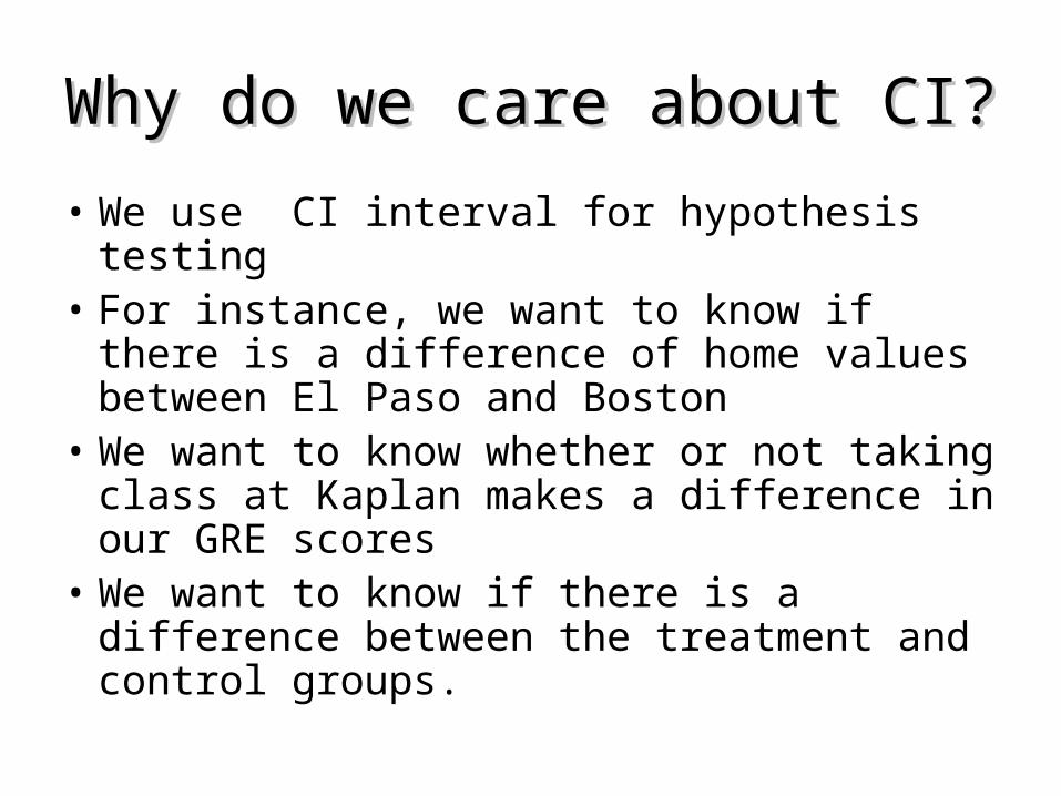
Why do we care about CI?Why do we care about CI?
• We use CI interval for hypothesis testing • For instance, we want to know if there is a
difference of home values between El Paso and Boston
• We want to know whether or not taking class at Kaplan makes a difference in our GRE scores
• We want to know if there is a difference between the treatment and control groups.
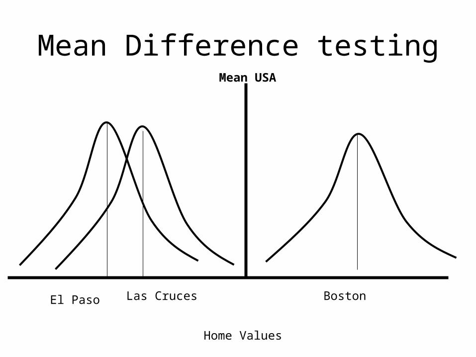
Mean Difference testing
Home Values
El Paso BostonLas Cruces
Mean USA
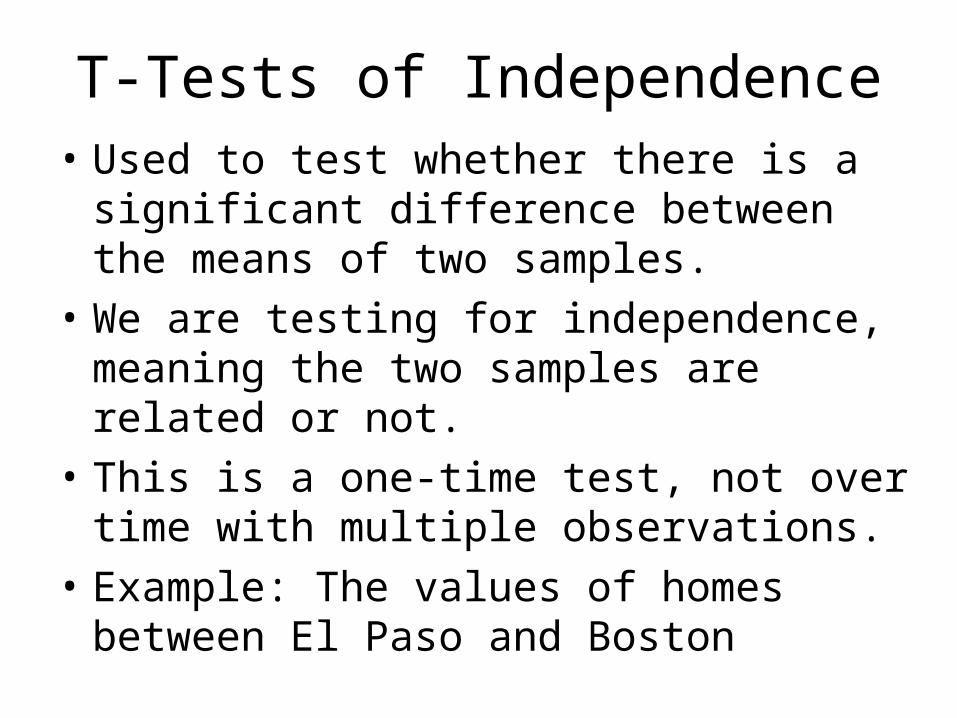
T-Tests of Independence• Used to test whether there is a significant
difference between the means of two samples.
• We are testing for independence, meaning the two samples are related or not.
• This is a one-time test, not over time with multiple observations.
• Example: The values of homes between El Paso and Boston
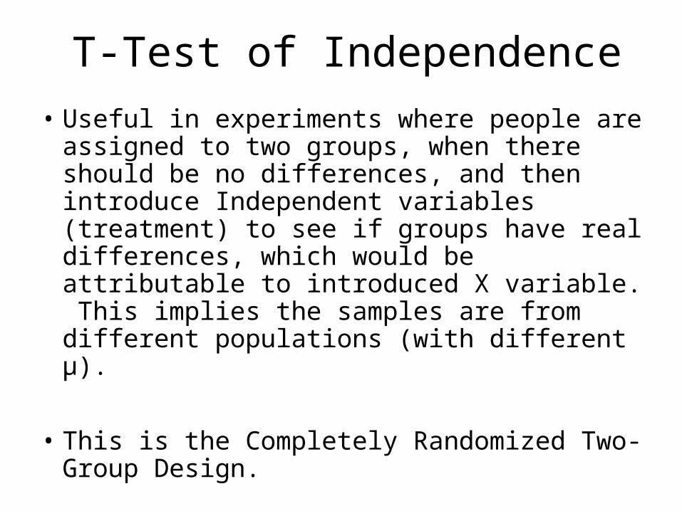
T-Test of Independence
• Useful in experiments where people are assigned to two groups, when there should be no differences, and then introduce Independent variables (treatment) to see if groups have real differences, which would be attributable to introduced X variable. This implies the samples are from different populations (with different μ).
• This is the Completely Randomized Two-Group Design.
T-Test of Independence
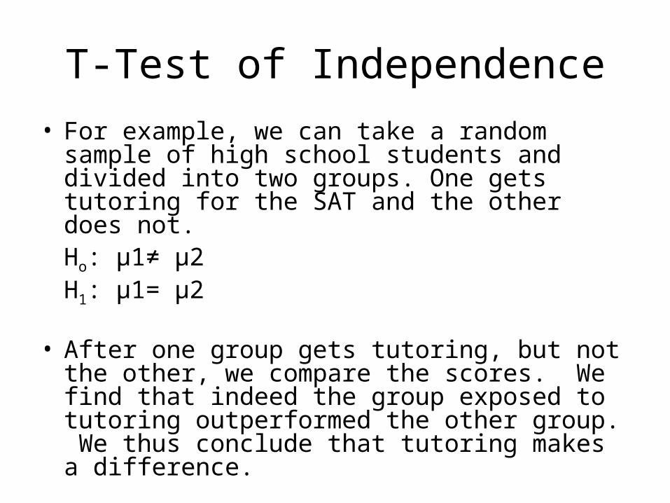
• For example, we can take a random sample of high school students and divided into two groups. One gets tutoring for the SAT and the other does not.
Ho: μ1≠ μ2 H1: μ1= μ2
• After one group gets tutoring, but not the other, we compare the scores. We find that indeed the group exposed to tutoring outperformed the other group. We thus conclude that tutoring makes a difference.
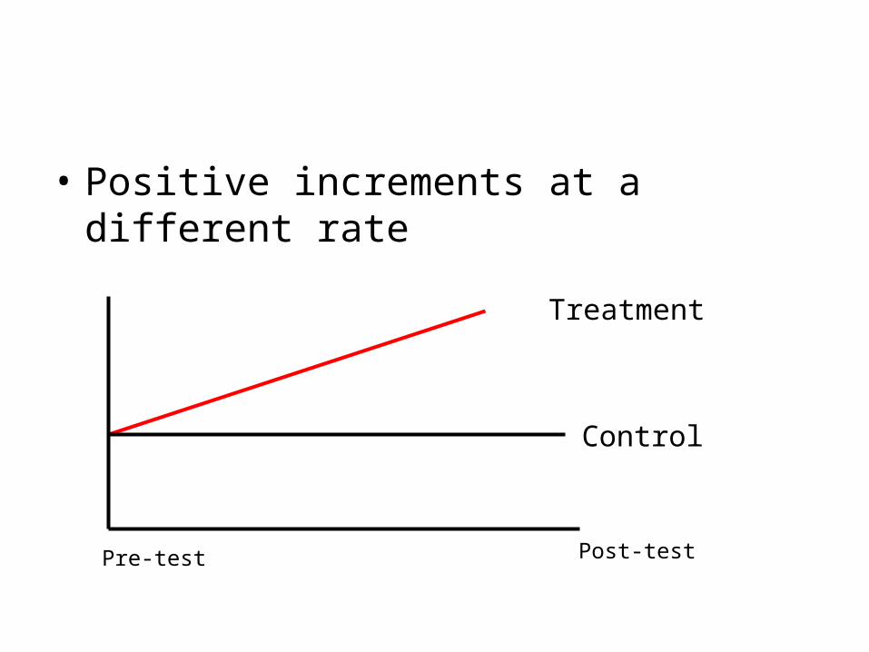
• Positive increments at a different rate
Treatment
Control
Pre-test Post-test
21
21
2
21
222
11
21
2)1()1(
nnnn
nnsnsn
XXt
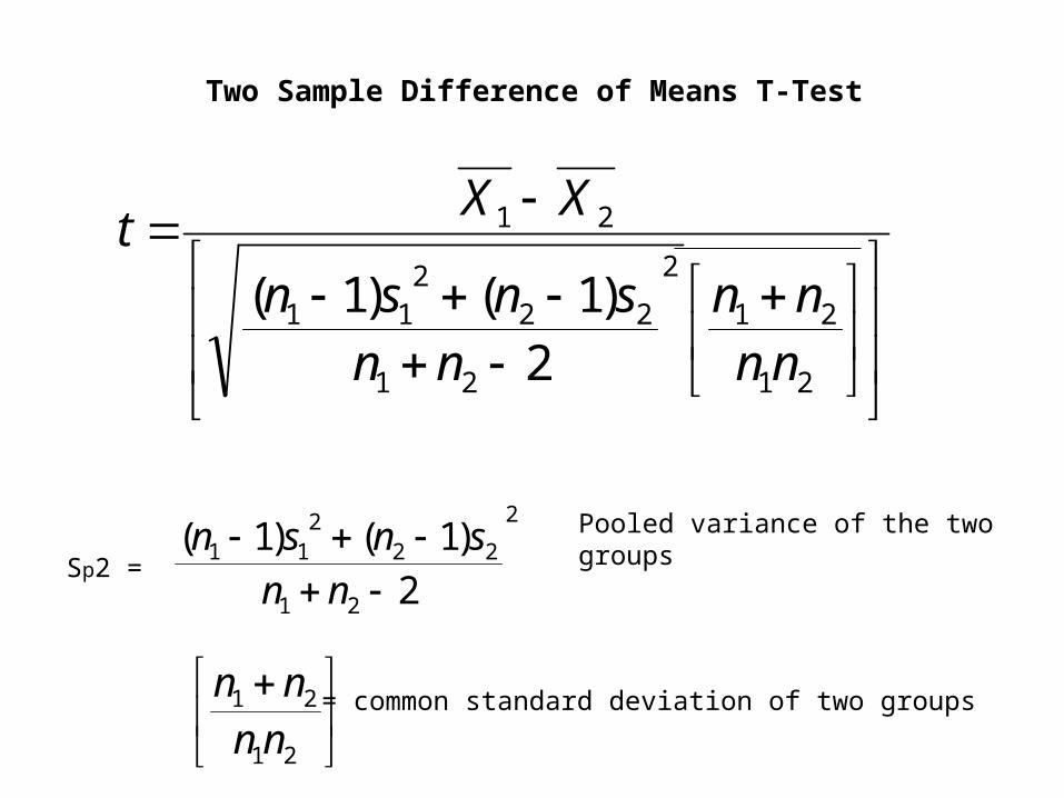
Two Sample Difference of Means T-Test
2
21
222
11
2
)1()1(
nn
snsnSp2 =
Pooled variance of the two groups
21
21
nn
nn = common standard deviation of two groups
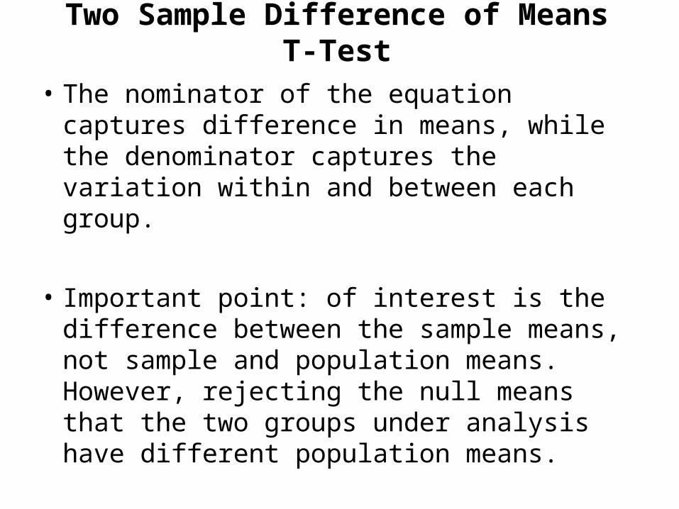
Two Sample Difference of Means T-Test
• The nominator of the equation captures difference in means, while the denominator captures the variation within and between each group.
• Important point: of interest is the difference between the sample means, not sample and population means. However, rejecting the null means that the two groups under analysis have different population means.
An example
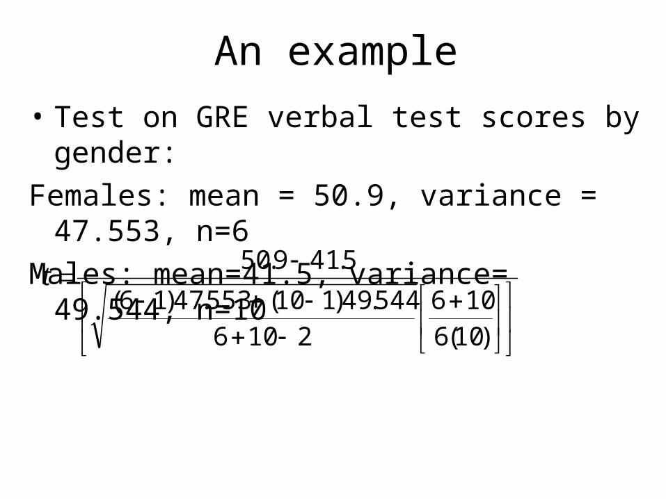
• Test on GRE verbal test scores by gender:
Females: mean = 50.9, variance = 47.553, n=6
Males: mean=41.5, variance= 49.544, n=10
)10(6
106
2106
544.49)110(553.47)16(
5.419.50t

)26667(.826.48
4.9t
02.13
4.9t
605.2608.3
4.9t Now what do we do with this
obtained value?

Steps of Testing and Significance
1. Statement of null hypothesis: if there is not one then how can you be wrong?
2. Set Alpha Level of Risk: .10, .05, .01
3. Selection of appropriate test statistic: T-test,
4. Computation of statistical value: get obtained value.
5. Compare obtained value to critical value: done for you for most methods in most statistical packages.
Steps of Testing and Significance
6. Comparison of the obtained and critical values.
7. If obtained value is more extreme than critical value, you may reject the null hypothesis. In other words, you have significant results.
8. If point seven above is not true, obtained is lower than critical, then null is not rejected.
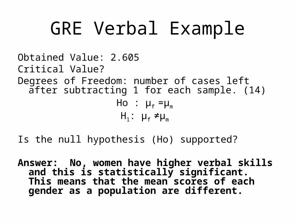
GRE Verbal Example
Obtained Value: 2.605Critical Value?Degrees of Freedom: number of cases left after subtracting
1 for each sample. (14)Ho : μf =μm H1: μf ≠μm
Is the null hypothesis (Ho) supported?
Answer: No, women have higher verbal skills and this is statistically significant. This means that the mean scores of each gender as a population are different.
Paired T-Tests• We use Paired T-Tests, test of
dependence, to examine a single sample subjects/units under two conditions, such as pretest - posttest experiment.
• For example, we can examine whether a group of students improves if they retake the GRE exam. The T-test examines if there is any significant difference between the two studies. If so, then possibly something like studying more made a difference.

Paired T-Tests• Unlike a test for independence, this test
requires that the two groups/samples being evaluated are dependent upon each other.
• For example, we can use a paired t-test to examine two sets of scores across time as long as they come from the same students.
• This is appropriate for a pre-test –post-test research design
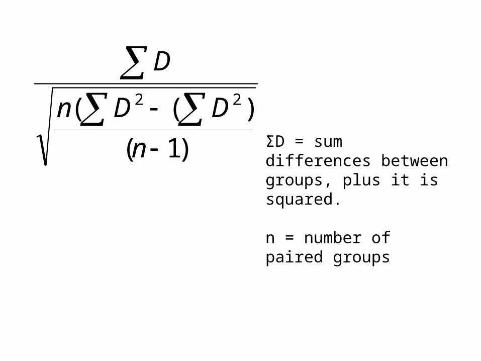
)1(
)(( 22
n
DDn
D
ΣD = sum differences between groups, plus it is squared.
n = number of paired groups
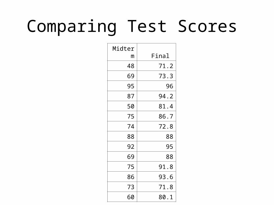
Comparing Test Scores Midterm Final
48 71.2
69 73.3
95 96
87 94.2
50 81.4
75 86.7
74 72.8
88 88
92 95
69 88
75 91.8
86 93.6
73 71.8
60 80.1
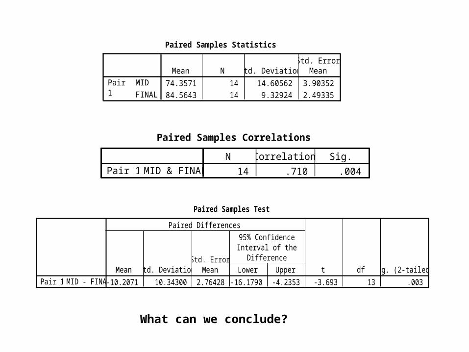
Paired Samples Statistics
74.3571 14 14.60562 3.90352
84.5643 14 9.32924 2.49335
MID
FINAL
Pair1
Mean N Std. DeviationStd. Error
Mean
Paired Samples Correlations
14 .710 .004MID & FINALPair 1N Correlation Sig.
Paired Samples Test
-10.2071 10.34300 2.76428 -16.1790 -4.2353 -3.693 13 .003MID - FINALPair 1Mean Std. Deviation
Std. ErrorMean Lower Upper
95% ConfidenceInterval of the
Difference
Paired Differences
t df Sig. (2-tailed)
What can we conclude?
![Author Manuscript NIH Public Access ‡, May L. Lam ... J Biol Chem.pdf · Ci/mmol) and [3H]CGP12177 (specific activity = 51 Ci/mmol) were from AmershamBiosciences. All other materials](https://static.fdocument.org/doc/165x107/5f9a3bd75b96fb195c761951/author-manuscript-nih-public-access-a-may-l-lam-j-biol-chempdf-cimmol.jpg)


![ChargeIndependent(CI)andChargeDependent(CD ... · arXiv:0806.0513v1 [nucl-ex] 3 Jun 2008 ChargeIndependent(CI)andChargeDependent(CD)correlationsasafunction of Centralityformed from∆φ∆η](https://static.fdocument.org/doc/165x107/5f920116e1ec56144512ce77/chargeindependentciandchargedependentcd-arxiv08060513v1-nucl-ex-3-jun.jpg)