
Inference for the Weibull Distribution - stat.washington.edu · Inference for the Weibull...
59
Inference for the Weibull Distribution Stat 498B Industrial Statistics Fritz Scholz May 22, 2008 1 The Weibull Distribution The 2-parameter Weibull distribution function is defined as F α,β (x)=1 - exp - x α β for x ≥ 0 and F α,β (x)=0 for t< 0. We also write X ∼W(α, β ) when X has this distribution function, i.e., P (X ≤ x)= F α,β (x). The parameters α> 0 and β> 0 are referred to as scale and shape parameter, respectively. The Weibull density has the following form f α,β (x)= F α,β (x)= d dx F α,β (x)= β α x α β-1 exp - x α β . For β = 1 the Weibull distribution coincides with the exponential distribution with mean α. In general, α represents the .632-quantile of the Weibull distribution regardless of the value of β since F α,β (α)=1 - exp(-1) ≈ .632 for all β> 0. Figure 1 shows a representative collection of Weibull densities. Note that the spread of the Weibull distributions around α gets smaller as β increases. The reason for this will become clearer later when we discuss the log-transform of Weibull random variables. The m th moment of the Weibull distribution is E(X m )= α m Γ(1 + m/β ) and thus the mean and variance are given by μ = E(X )= αΓ(1 + 1/β ) and σ 2 = α 2 Γ(1 + 2/β ) -{Γ(1 + 1/β )} 2 . Its p-quantile, defined by P (X ≤ x p )= p, is x p = α(- log(1 - p)) 1/β . For p =1 - exp(-1) ≈ .632 (i.e., - log(1 - p) = 1) we have x p = α regardless of β , as pointed out previously. For that reason one also calls α the characteristic life of the Weibull distribution. The term life comes from the common use of the Weibull distribution in modeling lifetime data. More on this later. 1
Transcript of Inference for the Weibull Distribution - stat.washington.edu · Inference for the Weibull...
Inference for the Weibull Distribution
Stat 498B Industrial Statistics
Fritz Scholz
May 22, 2008
1 The Weibull Distribution
The 2-parameter Weibull distribution function is defined as
Fα,β(x) = 1− exp
[−(x
α
)β]
for x ≥ 0 and Fα,β(x) = 0 for t < 0.
We also write X ∼ W(α, β) when X has this distribution function, i.e., P (X ≤ x) = Fα,β(x). Theparameters α > 0 and β > 0 are referred to as scale and shape parameter, respectively. The Weibulldensity has the following form
fα,β(x) = F ′α,β(x) =
d
dxFα,β(x) =
β
α
(x
α
)β−1
exp
[−(x
α
)β].
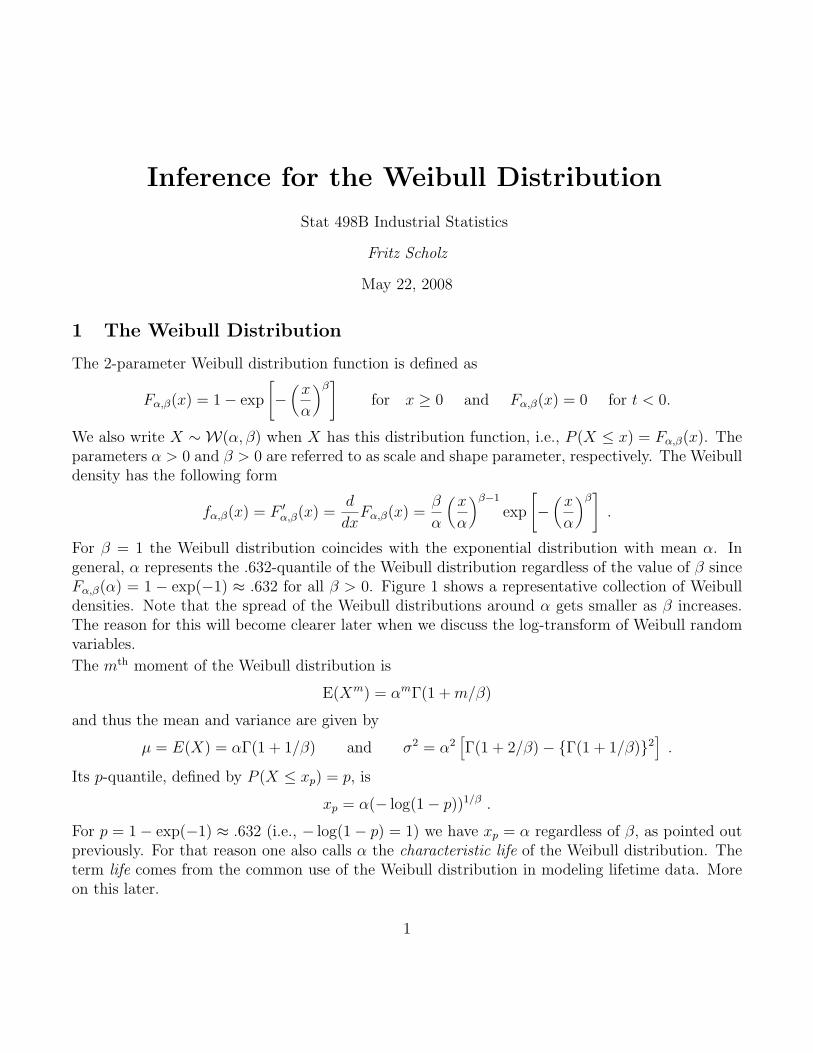
For β = 1 the Weibull distribution coincides with the exponential distribution with mean α. Ingeneral, α represents the .632-quantile of the Weibull distribution regardless of the value of β sinceFα,β(α) = 1 − exp(−1) ≈ .632 for all β > 0. Figure 1 shows a representative collection of Weibulldensities. Note that the spread of the Weibull distributions around α gets smaller as β increases.The reason for this will become clearer later when we discuss the log-transform of Weibull randomvariables.
The mth moment of the Weibull distribution is
E(Xm) = αmΓ(1 +m/β)
and thus the mean and variance are given by
µ = E(X) = αΓ(1 + 1/β) and σ2 = α2[Γ(1 + 2/β)− {Γ(1 + 1/β)}2
].
Its p-quantile, defined by P (X ≤ xp) = p, is
xp = α(− log(1− p))1/β .
For p = 1− exp(−1) ≈ .632 (i.e., − log(1− p) = 1) we have xp = α regardless of β, as pointed outpreviously. For that reason one also calls α the characteristic life of the Weibull distribution. Theterm life comes from the common use of the Weibull distribution in modeling lifetime data. Moreon this later.
1
Weibull densities
ββ1 == 0.5ββ2 == 1ββ3 == 1.5ββ4 == 2ββ5 == 3.6ββ6 == 7αα == 10000
αα
36.8%63.2%
Figure 1: A Collection of Weibull Densities with α = 10000 and Various Shapes
2
2 Minimum Closure and Weakest Link Property
The Weibull distribution has the following minimum closure property: IfX1, . . . , Xn are independentwith Xi ∼ W(αi, β), i = 1, . . . , n, then
P (min(X1, . . . , Xn) > t) = P (X1 > t, . . . , Xn > t) =n∏
i=1
P (Xi > t)
=n∏
i=1
exp
[−(t
αi
)β]
= exp
[−tβ
n∑i=1
1
αβi
]
= exp
[−(t
α?
)β]
with α? =
(n∑
i=1
1
αβi
)−1/β
,
i.e., min(X1, . . . , Xn) ∼ W(α?, β). This is reminiscent of the closure property for the normaldistribution under summation, i.e., if X1, . . . , Xn are independent with Xi ∼ N (µi, σ
2i ) then
n∑i=1
Xi ∼ N(
n∑i=1
µi,n∑
i=1
σ2i
).
This summation closure property plays an essential role in proving the central limit theorem: Sumsof independent random variables (not necessarily normally distributed) have an approximate normaldistribution, subject to some mild conditions concerning the distribution of such random variables.There is a similar result from Extreme Value Theory that says: The minimum of independent,identically distributed random variables (not necessarily Weibull distributed) has an approximateWeibull distribution, subject to some mild conditions concerning the distribution of such randomvariables. This is also referred to as the “weakest link” motivation for the Weibull distribution.
The Weibull distribution is appropriate when trying to characterize the random strength of materialsor the random lifetime of some system. This is related to the weakest link property as follows. Apiece of material can be viewed as a concatenation of many smaller material cells, each of which hasits random breaking strength Xi when subjected to stress. Thus the strength of the concatenatedtotal piece is the strength of its weakest link, namely min(X1, . . . , Xn), i.e., approximately Weibull.
Similarly, a system can be viewed as a collection of many parts or subsystems, each of which has arandom lifetime Xi. If the system is defined to be in a failed state whenever any one of its parts orsubsystems fails, then the system lifetime is min(X1, . . . , Xn), i.e., approximately Weibull.
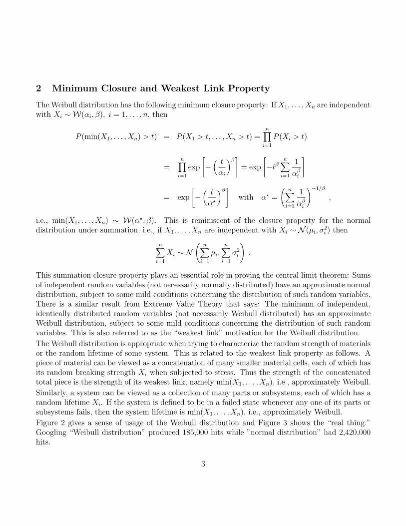
Figure 2 gives a sense of usage of the Weibull distribution and Figure 3 shows the “real thing.”Googling “Weibull distribution” produced 185,000 hits while ”normal distribution” had 2,420,000hits.
3
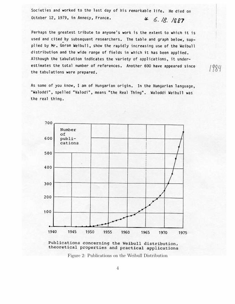
Figure 2: Publications on the Weibull Distribution
4
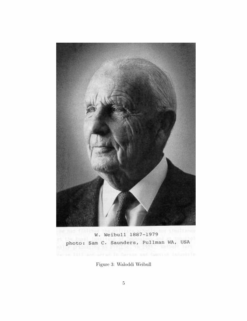
Figure 3: Waloddi Weibull
5

The Weibull distribution is very popular among engineers. One reason for this is that the Weibullcdf has a closed form which is not the case for the normal cdf Φ(x). However, in today’s computingenvironment one could argue that point since typically the computation of even exp(x) requirescomputing. That this can be accomplished on most calculators is also moot since many calculatorsalso give you Φ(x). Another reason for the popularity of the Weibull distribution among engi-neers may be that Weibull’s most famous paper, originally submitted to a statistics journal andrejected, was eventually published in an engineering journal: Waloddi Weibull (1951) “A statisticaldistribution function of wide applicability.” Journal of Applied Mechanics, 18, 293-297.
“. . . he tried to publish an article in a well-known British journal. At this time, the distri-bution function proposed by Gauss was dominating and was distinguishingly called the normaldistribution. By some statisticians it was even believed to be the only possible one. The arti-cle was refused with the comment that it was interesting but of no practical importance. Thatwas just the same article as the highly cited one published in 1951.” (Goran W. Weibull, 1981,http://www.garfield.library.upenn.edu/classics1981/A1981LD32400001.pdf)
Sam Saunders (1975): ‘Professor Wallodi (sic) Weibull recounted to me that the now famous paper ofhis “A Statistical Distribution of Wide Applicability”, in which was first advocated the “Weibull”distribution with its failure rate a power of time, was rejected by the Journal of the AmericanStatistical Association as being of no interrest. Thus one of the most influential papers in statisticsof that decade was published in the Journal of Applied Mechanics. See [35]. (Maybe that is thereason it was so influential!)’
3 The Hazard Function
The hazard function for any nonnegative random variable with cdf F (x) and density f(x) is definedas h(x) = f(x)/(1−F (x)). It is usually employed for distributions that model random lifetimes andit relates to the probability that a lifetime comes to an end within the next small time incrementof length d given that the lifetime has exceeded x so far, namely
P (x < X ≤ x+ d|X > x) =P (x < X ≤ x+ d)
P (X > x)=F (x+ d)− F (x)
1− F (x)≈ d× f(x)
1− F (x)= d× h(x) .
In the case of the Weibull distribution we have
h(x) =fα,β(x)
1− Fα,β(x)=β
α
(x
α
)β−1
.
Various other terms are used equivalently for the hazard function, such as hazard rate, failure rate(function), or force of mortality. In the case of the Weibull hazard rate function we observe that it
6
is increasing in x when β > 1, decreasing in x when β < 1 and constant when β = 1 (exponentialdistribution with memoryless property).
When β > 1 the part or system, for which the lifetime is modeled by a Weibull distribution, issubject to aging in the sense that an older system has a higher chance of failing during the nextsmall time increment d than a younger system.
For β < 1 (less common) the system has a better chance of surviving the next small time incrementd as it gets older, possibly due to hardening, maturing, or curing. Often one refers to this situationas one of infant mortality, i.e., after initial early failures the survival gets better with age. However,one has to keep in mind that we may be modeling parts or systems that consist of a mixture ofdefective or weak parts and of parts that practically can live forever. A Weibull distribution withβ < 1 may not do full justice to such a mixture distribution.
For β = 1 there is no aging, i.e., the system is as good as new given that it has survived beyond x,since for β = 1 we have
P (X > x+ h|X > x) =P (X > x+ h)
P (X > x)=
exp(−(x+ h)/α)
exp(−x/α)= exp(−h/α) = P (X > h) ,
i.e., it is again exponential with same mean α. One also refers to this as a random failure model inthe sense that failures are due to external shocks that follow a Poisson process with rate λ = 1/α.The random times between shocks are exponentially distributed with mean α. Given that there arek such shock events in an interval [0, T ] one can view the k occurrence times as being uniformlydistributed over the interval [0, T ], hence the allusion to random failures.
4 Location-Scale Property of log(X)
Another useful property, of which we will make strong use, is the following location-scale propertyof the log-transformed Weibull distribution. By that we mean that: X ∼ W(α, β) =⇒ log(X) = Yhas a location-scale distribution, namely its cumulative distribution function (cdf) is
P (Y ≤ y) = P (log(X) ≤ y) = P (X ≤ exp(y)) = 1− exp
−(exp(y)
α
)β
= 1− exp [− exp {(y − log(α))× β}] = 1− exp
[− exp
(y − log(α)
1/β
)]
= 1− exp[− exp
(y − u
b
)]with location parameter u = log(α) and scale parameter b = 1/β. The reason for referring to suchparameters this way is the following. If Z ∼ G(z) then Y = µ+ σZ ∼ G((y − µ)/σ) since
H(y) = P (Y ≤ y) = P (µ+ σZ ≤ y) = P (Z ≤ (y − µ)/σ) = G((y − µ)/σ) .
7

The form Y = µ+ σX should make clear the notion of location scale parameter, since Z has beenscaled by the factor σ and is then shifted by µ. Two prominent location-scale families are
1. Y = µ+ σZ ∼ N (µ, σ2), where Z ∼ N (0, 1) is standard normal with cdf G(z) = Φ(z)and thus Y has cdf H(y) = Φ((y − µ)/σ),
2. Y = u+ bZ where Z has the standard extreme value distribution with cdfG(z) = 1− exp(− exp(z)) for z ∈ R, as in our log-transformed Weibull example above.
In any such a location-scale model there is a simple relationship between the p-quantiles of Y andZ, namely yp = µ + σzp in the normal model and yp = u + bwp in the extreme value model (usingthe location and scale parameters u and b resulting from log-transformed Weibull data). We justillustrate this in the extreme value location-scale model.
p = P (Z ≤ wp) = P (u+ bZ ≤ u+ bwp) = P (Y ≤ u+ bwp) =⇒ yp = u+ bwp
with wp = log(− log(1− p)). Thus yp is a linear function of wp = log(− log(1− p)), the p-quantileof G. While wp is known and easily computable from p, the same cannot be said about yp, sinceit involves the typically unknown parameters u and b. However, for appropriate pi = (i − .5)/none can view the ith ordered sample value Y(i) (Y(1) ≤ . . . ≤ Y(n)) as a good approximation for ypi
.Thus the plot of Y(i) against wpi
should look approximately linear. This is the basis for Weibullprobability plotting (and the case of plotting Y(i) against zpi
for normal probability plotting), a veryappealing graphical procedure which gives a visual impression of how well the data fit the assumedmodel (normal or Weibull) and which also allows for a crude estimation of the unknown locationand scale parameters, since they relate to the slope and intercept of the line that may be fitted tothe perceived linear point pattern. For more in relation to Weibull probability plotting we refer toScholz (2008).
5 Maximum Likelihood Estimation
There are many ways to estimate the parameters θ = (α, β) based on a random sampleX1, . . . , Xn ∼W(α, β). Maximum likelihood estimation (MLE) is generally the most versatile and popularmethod. Although MLE in the Weibull case requires numerical methods and a computer, that is nolonger an issue in today’s computing environment. Previously, estimates that could be computedby hand had been investigated, but they are usually less efficient than mle’s (estimates derived byMLE). By efficient estimates we loosely refer to estimates that have the smallest sampling variance.MLE tends to be efficient, at least in large samples. Furthermore, under regularity conditions MLEproduces estimates that have an approximate normal distribution in large samples.
8
When X1, . . . , Xn ∼ Fθ(x) with density fθ(x) then the maximum likelihood estimate of θ is thatvalue θ = θ = θ(x1, . . . , xn) which maximizes the likelihood
L(x1, . . . , xn, θ) =n∏
i=1
fθ(xi)
over θ, i.e., which gives highest local probability to the observed sample (X1, . . . , Xn) = (x1, . . . , xn)
L(x1, . . . , xn, θ) = supθ
{n∏
i=1
fθ(xi)
}.
Often such maximizing values θ are unique and one can obtain them by solving, i.e.,
∂
∂θj
n∏i=1
fθ(xi) = 0 j = 1, . . . , k ,
where k is the number of parameters involved in θ = (θ1, . . . , θk). These above equations reflect thefact that a smooth function has a horizontal tangent plane at its maximum (minimum or saddlepoint). Thus solving such equations is necessary but not sufficient, since it still needs to be shownthat it is the location of a maximum.
Since taking derivatives of a product is tedious (product rule) one usually resorts to maximizingthe log of the likelihood, i.e.,
`(x1, . . . , xn, θ) = log (L(x1, . . . , xn, θ)) =n∑
i=1
log (fθ(xi))
since the value of θ that maximizes L(x1, . . . , xn, θ) is the same as the value that maximizes`(x1, . . . , xn, θ), i.e.,
`(x1, . . . , xn, θ) = supθ
{n∑
i=1
log (fθ(xi))
}.
It is a lot simpler to deal with the likelihood equations
∂
∂θj
`(x1, . . . , xn, θ) =∂
∂θj
n∑i=1
log(fθ(xi)) =n∑
i=1
∂
∂θj
log(fθ(xi)) = 0 j = 1, . . . , k
when solving for θ = θ = θ(x1, . . . , xn).
In the case of a normal random sample we have θ = (µ, σ) with k = 2 and the unique solution ofthe likelihood equations results in the explicit expressions
µ = x =n∑
i=1
xi/n and σ =
√√√√ n∑i=1
(xi − x)2/n and thus θ = (µ, σ) .
9
In the case of a Weibull sample we take the further simplifying step of dealing with the log-transformed sample (y1, . . . , yn) = (log(x1), . . . , log(xn)). Recall that Yi = log(Xi) has cdf F (y) =1 − exp(− exp((x − u)/b)) = G((y − u)/b) with G(z) = 1 − exp(− exp(z)) with g(z) = G′(z) =exp(z − exp(z)). Thus
f(y) = F ′(y) =d
dyF (y) =
1
bg((y − u)/b))
with
log(f(y)) = − log(b) +y − u
b− exp
(y − u
b
).
As partial derivatives of log(f(y)) with respect to u and b we get
∂
∂ulog(f(y)) = −1
b+
1
bexp
(y − u
b
)∂
∂blog(f(y)) = − 1
b− 1
b
y − u
b+
1
b
y − u
bexp
(y − u
b
)and thus as likelihood equations
0 = −nb
+1
b
n∑i=1
exp(yi − u
b
)or
n∑i=1
exp(yi − u
b
)= n or exp(u) =
[1
n
n∑i=1
exp(yi
b
)]b
,
0 = − n
b− 1
b
n∑i=1
yi − u
b+
1
b
n∑i=1
yi − u
bexp
(yi − u
b
).
i.e., we have a solution u = u once we have a solution b = b. Substituting this expression for exp(u)into the second likelihood equation we get (after some cancelation and manipulation)
0 =
∑ni=1 yi exp(yi/b)∑n
i=1 exp(yi/b)− b− 1
n
n∑i=1
yi .
Analyzing the solvability of this equation is more convenient in terms of β = 1/b and we thus write
0 =n∑
i=1
yiwi(β)− 1
β− y where wi(β) =
exp(yiβ)∑nj=1 exp(yjβ)
withn∑
i=1
wi(β) = 1 .
Note that the derivative of these weights with respect to β take the following form
w′i(β) =
d
dβwi(β) = yiwi(β)− wi(β)
n∑j=1
yjwj(β) .
10
Hence
d
dβ
{n∑
i=1
yiwi(β)− 1
β− y
}=
n∑i=1
yiw′i(β) +
1
β2=
n∑i=1
y2iwi(β)−
n∑j=1
yjwj(β)
2
+1
β2> 0
since
varw(y) =n∑
i=1
y2iwi(β)−
n∑j=1
yjwj(β)
2
= Ew(y2)− [Ew(y)]2 ≥ 0
can be interpreted as a variance of the n values of y = (y1, . . . , yn) with weights or probabilities givenby w = (w1(β), . . . , wn(β)). Thus the reduced second likelihood equation
∑yiwi(β)− 1/β − y = 0
has a unique solution (if it has a solution at all) since the the equation’s left side is strictly increasing.
Note that wi(β) → 1/n as β → 0. Thus∑yiwi(β)− 1/β − y ≈ −1/β → −∞ as β → 0.
Furthermore, with M = max(y1, . . . , yn) and β →∞ we have
wi(β) = exp(β(yi−M))/n∑
j=1
exp(β(yj−M)) → 0 when yi < M and wi(β) → 1/r when yi = M,
where r ≥ 1 is the number of yi coinciding with M . Thus∑yiwi(β)− 1/β − y ≈M − 1/β − y →M − y > 0 as β →∞
where M − y > 0 assumes that not all yi coincide (a degenerate case with probability 0). That thisunique solution corresponds to a maximum and thus a unique global maximum takes some extraeffort and we refer to Scholz (1996) for an even more general treatment that covers Weibull analysiswith censored data and covariates.
However, a somewhat loose argument can be given as follows. If we consider the likelihood of thelog-transformed Weibull data we have
L(y1, . . . , yn, u, b) =1
bn
n∏i=1
g(yi − u
b
).
Contemplate this likelihood for fixed y = (y1, . . . , yn) and for parameters u with |u| → ∞ (thelocation moves away from all observed data values y1, . . . , yn) and b with b→ 0 (the spread becomesvery concentrated on some point and cannot simultaneously do so at all values y1, . . . , yn, unlessthey are all the same, excluded as a zero probability degeneracy) and b → ∞ (in which case allprobability is diffused thinly over the whole half plane {(u, b) : u ∈ R, b > 0}), it is then easily seenthat this likelihood approaches zero in all cases. Since this likelihood is positive everywhere (butapproaching zero near the fringes of the parameter space, the above half plane) it follows that it
11
must have a maximum somewhere with zero partial derivatives. We showed there is only one suchpoint (uniqueness of the solution to the likelihood equations) and thus there can only be one unique(global) maximum, which then is also the unique maximum likelihood estimate θ = (u, b).
In solving 0 =∑yi exp(yi/b)/
∑exp(yi/b) − b − y it is numerically advantageous to solve the
equivalent equation 0 =∑yi exp((yi−M)/b)/
∑exp((yi−M)/b)−b−y where M = max(y1, . . . , yn).
This avoids overflow or accuracy loss in the exponentials when the yi tend to be large.
The above derivations go through with very little change when instead of observing a full sampleY1, . . . , Yn we only observe the r ≥ 2 smallest sample values Y(1) < . . . < Y(r). Such data is referredto as type II censored data. This situation typically arises in a laboratory setting when severalunits are put on test (subjected to failure exposure) simultaneously and the test is terminated(or evaluated) when the first r units have failed. In that case we know the first r failure timesX(1) < . . . < X(r) and thus Y(i) = log(X(i)), i = 1, . . . , r, and we know that the lifetimes of theremaining units exceed X(r) or that Y(i) > Y(r) for i > r. The advantage of such data collection isthat we do not have to wait until all n units have failed. Furthermore, if we put a lot of units ontest (high n) we increase our chance of seeing our first r failures before a fixed time y. This is asimple consequence of the following binomial probability statement:
P (Y (r) ≤ y) = P (at least r failures ≤ y in n trials) =n∑
i=r
(n
i
)P (Y ≤ y)i(1− P (Y ≤ y))n−i
which is strictly increasing in n for any fixed y and r ≥ 1 (exercise).
The joint density of Y(1), . . . , Y(n) at (y1, . . . , yn) with y1 < . . . < yn is
f(y1, . . . , yn) = n!n∏
i=1
1
bg(yi − u
b
)= n!
n∏i=1
f(yi)
where the multiplier n! just accounts for the fact that all n! permutations of y1, . . . , yn could havebeen the order in which these values were observed and all of these orders have the same density(probability). Integrating out yn > yn−1 > . . . > yr+1(> yr) and using F (y) = 1−F (y) we get aftern− r successive integration steps the joint density of the first r failure times y1 < . . . < yr as
f(y1, . . . , yn−1) = n!n−1∏i=1
f(yi)×∫ ∞
yn−1
f(yn)dyn = n!n−1∏i=1
f(yi)F (yn−1)
f(y1, . . . , yn−2) = n!n−2∏i=1
f(yi)×∫ ∞
yn−2
f(yn−1)F (yn−1)dyn−1 = n!n−2∏i=1
f(yi)×1
2F 2(yn−2)
f(y1, . . . , yn−3) = n!n−3∏i=1
f(yi)×∫ ∞
yn−3
f(yn−2)F2(yn−2)/2dyn−2 = n!
n−3∏i=1
f(yi)×1
3!F 3(yn−3)
12
. . .
f(y1, . . . , yr) = n!r∏
i=1
f(yi)×1
(n− r)!F n−r(yr) =
[n!
(n− r)!
r∏i=1
f(yi)
]× [1− F (yr)]
n−r
= r!r∏
i=1
1
bg(yi − u
b
)×(n
r
) [1−G
(yr − u
b
)]n−r
with log-likelihood
`(y1, . . . , yr, u, b) = log
(n!
(n− r)!
)− r log(b) +
r∑i=1
yi − u
b−
r∑i=1
? exp(yi − u
b
)
where we use the notationr∑
i=1
? xi =r∑
i=1
xi + (n− r)xr .
The likelihood equations are
0 =∂
∂u`(y1, . . . , yr, u, b) = −r
b+
1
b
r∑i=1
? exp(yi − u
b
)or exp(u) =
[1
r
r∑i=1
? exp(yi
b
)]b
0 =∂
∂b`(y1, . . . , yr, u, b) = − r
b− 1
b
r∑i=1
yi − u
b+
1
b
r∑i=1
? yi − u
bexp
(yi − u
b
)
where again the transformed first equation gives us a solution u once we have a solution b for b.Using this in the second equation it transforms to a single equation in b alone, namely
r∑i=1
? yi exp(yi/b)
/r∑
i=1
? exp(yi/b)− b− 1
r
r∑i=1
yi = 0 .
Again it is advisable to use the equivalent but computationally more stable form
r∑i=1
? yi exp((yi − yr)/b)
/r∑
i=1
? exp((yi − yr)/b)− b− 1
r
r∑i=1
yi = 0 .
As in the complete sample case one sees that this equation has a unique solution b and that (u, b)gives the location of the (unique) global maximimum of the likelihood function, i.e., (u, b) are themle’s.
13

6 Computation of Maximum Likelihood Estimates in R
The computation of the mle’s of the Weibull parameters α and β is facilitated by the functionsurvreg which is part of the R package survival. Here survreg is used in its most basic form inthe context of Weibull data (full sample or type II censored Weibull data). survreg does a wholelot more than compute the mle’s but we will not deal with these aspects here, at least for now.The following is an R function, called Weibull.mle, that uses survreg to compute these estimates.Note that it tests for the existence of survreg before calling it. This function is part of the R workspace that is posted on the class web site.
Weibull.mle <- function (x=NULL,n=NULL){
# This function computes the maximum likelihood estimates of alpha and beta
# for complete or type II censored samples assumed to come from a 2-parameter
# Weibull distribution. Here x is the sample, either the full sample or the first
# r observations of a type II censored sample. In the latter case one must specify
# the full sample size n, otherwise x is treated as a full sample.
# If x is not given then a default full sample of size n=10, namely
# c(7,12.1,22.8,23.1,25.7,26.7,29.0,29.9,39.5,41.9) is analyzed and the returned
# results should be
# $mles
# alpha.hat beta.hat
# 28.914017 2.799793
#
# In the type II censored usage
# Weibull.mle(c(7,12.1,22.8,23.1,25.7),10)
# $mles
# alpha.hat beta.hat
# 30.725992 2.432647
if(is.null(x))x <- c(7,12.1,22.8,23.1,25.7,26.7,29.0,29.9,39.5,41.9)
r <- length(x)
if(is.null(n)){n<-r}else{if(r>n||r<2){
return("x must have length r with: 2 <= r <= n")}}
xs <- sort(x)
if(!exists("survreg"))library(survival)
#tests whether survival package is loaded, if not, then it loads survival
if(r<n){
statusx <- c(rep(1,r),rep(0,n-r))
dat.weibull <- data.frame(c(xs,rep(xs[r],n-r)),statusx)
14
}else{statusx <- rep(1,n)
dat.weibull <- data.frame(xs,statusx)}
names(dat.weibull)<-c("time","status")
out.weibull <- survreg(Surv(time,status)~1,dist="weibull",data=dat.weibull)
alpha.hat <- exp(out.weibull$coef)
beta.hat <- 1/out.weibull$scale
parms <- c(alpha.hat,beta.hat)
names(parms)<-c("alpha.hat","beta.hat")
list(mles=parms)}
Note that survreg analyzes objects of class Surv. Here such an object is created by the functionSurv and it basically adjoins the failure times with a status vector of same length. The statusis 1 when a time corresponds to an actual failure time. It is 0 when the corresponding time isa censoring time, i.e., we only know that the unobserved actual failure time exceeds the reportedcensoring time. In the case of type II censored data these censoring times equal the rth largestfailure time.
To get a sense of the calculation speed of this function we ran Weibull.mle a 1000 times, whichtells us that the time to compute the mle’s in a sample of size n = 10 is roughly 5.91/1000 = .00591.This fact plays a significant role later on in the various inference procedures which we will discuss.
system.time(for(i in 1:1000){Weibull.mle(rweibull(10,1))})
user system elapsed
5.79 0.00 5.91
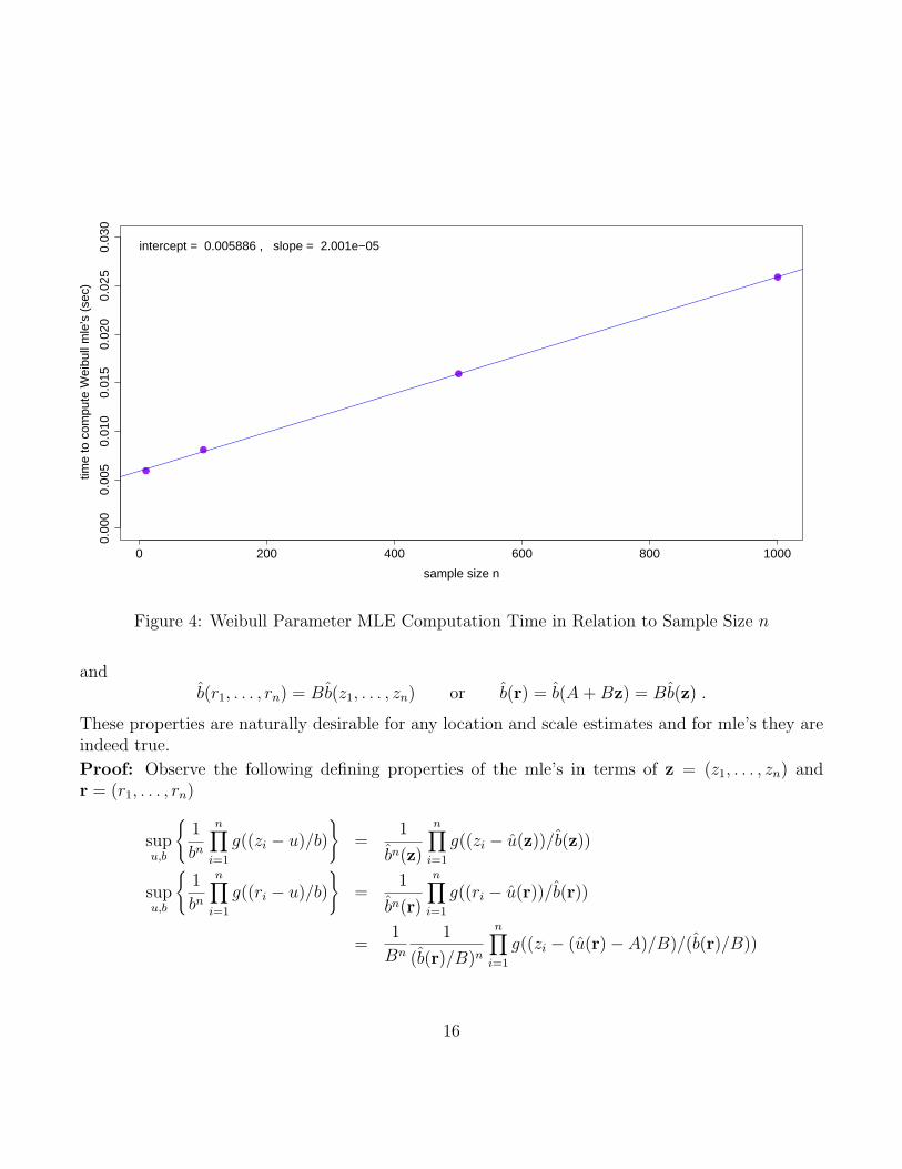
For n = 100, 500, 1000 the elapsed times came to 8.07, 15.91 and 25.87, respectively. The relationshipof computing time to n appears to be quite linear, but with slow growth, as Figure 4 shows.
7 Location and Scale Equivariance of Maximum Likelihood Estimates
The maximum likelihood estimates u and b of the location and scale parameters u and b have thefollowing equivariance properties which will play a strong role in the later pivot construction andresulting confidence intervals.
Based on data z = (z1, . . . , zn) we denote the estimates of u and b more explicitly by u(z1, . . . , zn) =u(z) and b(z1, . . . , zn) = b(z). If we transform z to r = (r1, . . . , rn) with ri = A+Bzi, where A ∈ Rand B > 0 are arbitrary constant, then
u(r1, . . . , rn) = A+Bu(z1, . . . , zn) or u(r) = u(A+Bz) = A+Bu(z)
15
●
●
●
●
0 200 400 600 800 1000
0.00
00.
005
0.01
00.
015
0.02
00.
025
0.03
0
sample size n
time
to c
ompu
te W
eibu
ll m
le's
(se
c)
intercept = 0.005886 , slope = 2.001e−05
Figure 4: Weibull Parameter MLE Computation Time in Relation to Sample Size n
andb(r1, . . . , rn) = Bb(z1, . . . , zn) or b(r) = b(A+Bz) = Bb(z) .
These properties are naturally desirable for any location and scale estimates and for mle’s they areindeed true.
Proof: Observe the following defining properties of the mle’s in terms of z = (z1, . . . , zn) andr = (r1, . . . , rn)
supu,b
{1
bn
n∏i=1
g((zi − u)/b)
}=
1
bn(z)
n∏i=1
g((zi − u(z))/b(z))
supu,b
{1
bn
n∏i=1
g((ri − u)/b)
}=
1
bn(r)
n∏i=1
g((ri − u(r))/b(r))
=1
Bn
1
(b(r)/B)n
n∏i=1
g((zi − (u(r)− A)/B)/(b(r)/B))
16
but also
supu,b
{1
bn
n∏i=1
g((ri − u)/b)
}= sup
u,b
{1
bn
n∏i=1
g((A+Bzi − u)/b)
}
= supu,b
{1
Bn
1
(b/B)n
n∏i=1
g((zi − (u− A)/B)/(b/B))
}u = (u− A)/B
b = b/B⇒ = sup
u,b
{1
Bn
1
bn
n∏i=1
g((zi − u)/b)
}=
1
Bn
1
bn(z)
n∏i=1
g((zi − u(z))/b(z))
Thus by the uniqueness of the mle’s we have
u(z) = (u(r)− A)/B and b(z) = b(r)/B
oru(r) = u(A+Bz) = A+Bu(z) and b(r) = b(A+Bz) = Bb(z) q.e.d.
The same equivariance properties hold for the mle’s in the context of type II censored samples, asis easily verified.
8 Tests of Fit Based on the Empirical Distribution Function
Relying on subjective assessment of linearity in Weibull probability plots in order to judge whethera sample comes from a 2-parameter Weibull population takes a fair amount of experience. It issimpler and more objective to employ a formal test of fit which compares the empirical distributionfunction Fn(x) of a sample with the fitted Weibull distribution function F (x) = Fα,β(x) using oneof several common discrepancy metrics.
The empirical distribution function (EDF) of a sample X1, . . . , Xn is defined as
Fn(x) =# of observations ≤ x
n=
1
n
n∑i=1
I{Xi≤x}
where IA = 1 when A is true, and IA = 0 when A is false. The fitted Weibull distribution function(using mle’s α and β) is
F (x) = Fα,β(x) = 1− exp
(−(x
α
)β).
From the law of large numbers (LLN) we see that for any x we have that Fn(x) −→ Fα,β(x) as
n −→∞. Just view Fn(x) as a binomial proportion or as an average of Bernoulli random variables.
17
From MLE theory we also know that F (x) = Fα,β(x) −→ Fα,β(x) as n −→ ∞ (also derived fromthe LLN).
Since the limiting cdf Fα,β(x) is continuous in x one can argue that these convergence statementscan be made uniformly in x, i.e.,
supx|Fn(x)− Fα,β(x)| −→ 0 and sup
x|Fα,β(x)− Fα,β(x)| −→ 0 as n −→∞
and thus supx|Fn(x)−Fα,β(x)| −→ 0 as n −→∞ for all α > 0 and β > 0.
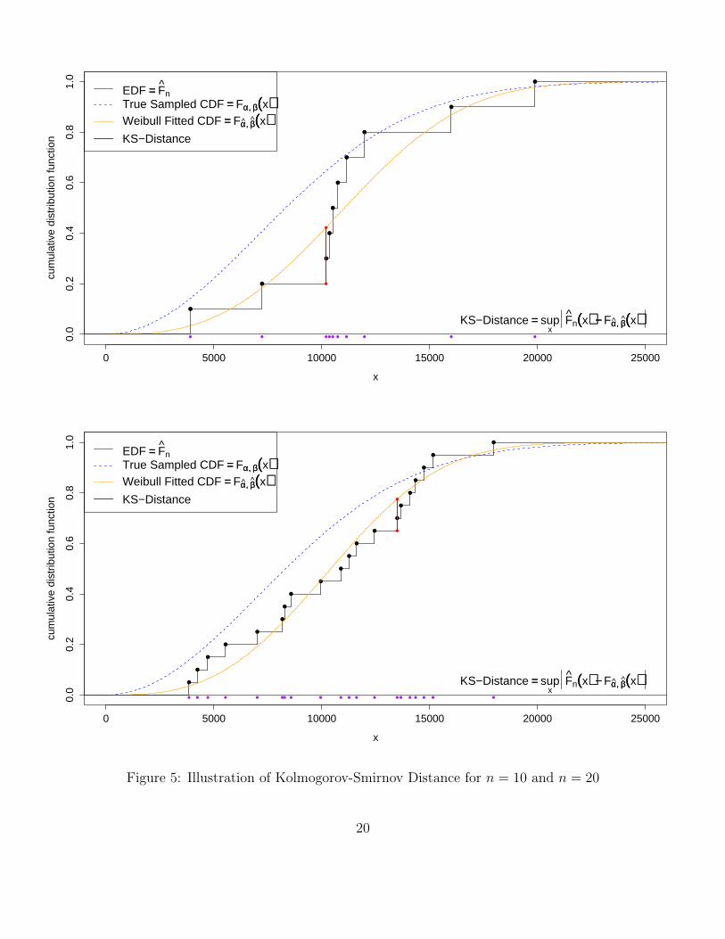
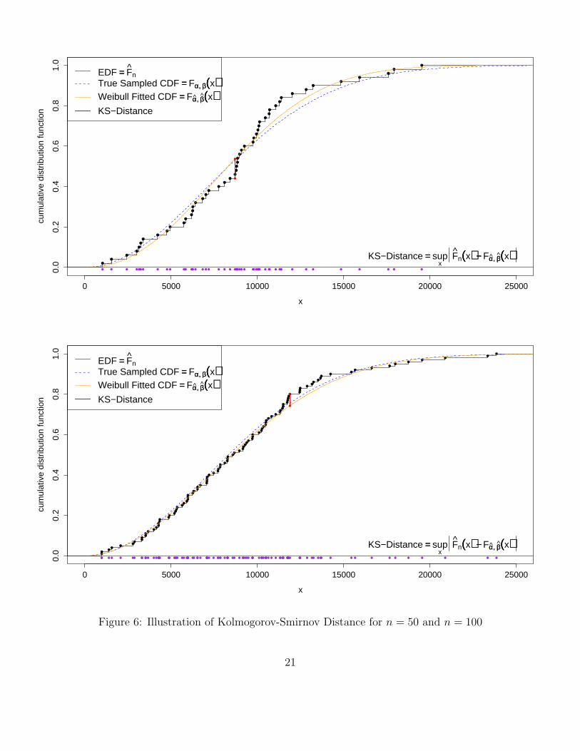
The distance DKS(F,G) = supx|F (x)−G(x)|
is known as the Kolmogorov-Smirnov distance between two cdf’s F and G.
Figures 5 and 6 give illustrations of this Kolmogorov-Smirnov distance between EDF and fittedWeibull distribution and show the relationship between sampled true Weibull distribution, fittedWeibull distribution, and empirical distribution function.
Some comments:
1. It can be noted that the closeness between Fn(x) and Fα,β(x) is usually more pronouncedthan their respective closeness to Fα,β(x), in spite of the sequence of the above convergencestatements.
2. This can be understood from the fact that both Fn(x) and Fα,β(x) fit the data, i.e., try togive a good representation of the data. The fit of the true distribution, although being theorigin of the data, is not always good due to sampling variation.
3. The closeness between all three distributions improves as n gets larger.
Several other distances between cdf’s F and G have been proposed and investigated in the literature.We will only discuss two of them, the Cramer-von Mises distance DCvM and the Anderson-Darlingdistance DAD. They are defined respectively as follows
DCvM(F,G) =∫ ∞
−∞(F (x)−G(x))2 dG(x) =
∫ ∞
−∞(F (x)−G(x))2 g(x) dx
and
DAD(F,G) =∫ ∞
−∞
(F (x)−G(x))2
G(x)(1−G(x))dG(x) =
∫ ∞
−∞
(F (x)−G(x))2
G(x)(1−G(x))g(x) dx .
Rather than focussing on the very local phenomenon of a maximum discrepancy at some point x asin DKS, these alternate distances or discrepancy metrics integrate these distances in squared formover all x, weighted by g(x) in the case of DCvM(F,G) and by g(x)/[G(x)(1 − G(x))] in the case
18
DAD(F,G). In the latter case, the denominator increases the weight in the tails of theG distribution,i.e., compensates to some extent for the tapering off in the density g(x). Thus DAD(F,G) is favoredin situations where judging tail behavior is important, e.g., in risk situations. Because of theintegration nature of these last two metrics they have more global character. There is no easygraphical representation of these metrics, except to suggest that when viewing the previous figuresillustrating DKS one should look at all vertical distances (large and small) between Fn(x) and F (x),square them and accumulate these squares in the appropriately weighted fashion. For example,when one cdf is shifted relative to the other by a small amount (no large vertical discrepancy),these small vertical discrepancies (squared) will add up and indicate a moderately large differencebetween the two compared cdf’s.
We point out the asymmetric nature of these last two metrics, i.e., we typically have
DCvM(F,G) 6= DCvM(G,F ) and DAD(F,G) 6= DAD(G,F ) .
When using these metrics for tests of fit one usually takes the cdf with a density (the modeldistribution to be tested) as the one with respect to which the integration takes place, while theother cdf is taken to be the EDF.
As complicated as these metrics may look at first glance, their computation is quite simple. Wewill give the following computational expressions (without proof):
DKS(Fn(x), F (x)) = D = max[max
{i/n− V(i)
}, max
{V(i) − (i− 1)/n
}]where V(1) ≤ . . . ≤ V(n) are the ordered values of Vi = F (Xi), i = 1, . . . , n.
For the other two test of fit criteria we have
DCvM(Fn(x), F (x)) = W 2 =n∑
i=1
{V(i) −
2i− 1
2n
}2
+1
12n
and
DAD(Fn(x), F (x)) = A2 = −n− 1
n
n∑i=1
(2i− 1)[log(V(i)) + log(1− V(n−i+1))
].
In order to carry out these tests of fit we need to know the null distributions of D, W 2 and A2.Quite naturally we would reject the hypothesis of a sampled Weibull distribution whenever D orW 2 or A2 are too large. The null distribution of D, W 2 and A2 does not depend on the unknownparameters α and β, being estimated by α and β in Vi = F (Xi) = Fα,β(Xi). The reason for thisis that the Vi have a distribution that is independent of the unknown parameters α and β. This isseen as follows. Using our prior notation we write log(Xi) = Yi = u+ bZi and since
19
0 5000 10000 15000 20000 25000
0.0
0.2
0.4
0.6
0.8
1.0
x
cum
ulat
ive
dist
ribut
ion
func
tion
●
●
●
●
●
●
●
●
●
●
● ● ● ● ● ● ● ● ● ●
●
●
EDF == FnTrue Sampled CDF == Fαα,, ββ((x))Weibull Fitted CDF == Fαα,, ββ((x))KS−Distance
KS−Distance == supx
Fn((x)) −− Fαα,, ββ((x))
0 5000 10000 15000 20000 25000
0.0
0.2
0.4
0.6
0.8
1.0
x
cum
ulat
ive
dist
ribut
ion
func
tion
●
●
●
●
●
●
●
●
●
●
●
●
●
●
●
●
●
●
●
●
● ● ● ● ● ● ● ● ● ● ● ● ● ● ● ● ● ● ● ●
●
●
EDF == FnTrue Sampled CDF == Fαα,, ββ((x))Weibull Fitted CDF == Fαα,, ββ((x))KS−Distance
KS−Distance == supx
Fn((x)) −− Fαα,, ββ((x))
Figure 5: Illustration of Kolmogorov-Smirnov Distance for n = 10 and n = 20
20
0 5000 10000 15000 20000 25000
0.0
0.2
0.4
0.6
0.8
1.0
x
cum
ulat
ive
dist
ribut
ion
func
tion
●
●
●
●
●
●
●
●
●
●
●
●
●
●
●
●
●
●
●
●
●
●
●
●
●
●
●
●
●
●
●
●
●
●
●
●
●
●
●
●
●
●
●
●
●
●
●
●
●
●
● ● ● ● ●● ● ● ● ● ●● ●●● ● ● ● ● ● ● ● ●●●●● ● ● ● ●● ●●●● ● ●● ● ●● ● ● ● ● ● ● ● ●
●
●
EDF == FnTrue Sampled CDF == Fαα,, ββ((x))Weibull Fitted CDF == Fαα,, ββ((x))KS−Distance
KS−Distance == supx
Fn((x)) −− Fαα,, ββ((x))
0 5000 10000 15000 20000 25000
0.0
0.2
0.4
0.6
0.8
1.0
x
cum
ulat
ive
dist
ribut
ion
func
tion
●●
●●
●●
●●●
●●
●●
●●●●●
●●
●●●●
●●
●●●●
●●
●●
●●●●●
●●
●●
●●
●●●●
●●
●●●
●●
●●●●
●●●
●●●●
●●
●●●
●●●
●●●●●
●●●
●●
●●
●●
●●
●●
●●
●●
●●
●
●● ● ● ● ●● ●● ●● ● ● ● ●●●● ●● ●●●● ●● ●●●● ●● ●● ● ●●●●● ● ●●●● ● ●●● ●● ● ●●●●● ●●● ● ●●● ●●● ● ● ● ●● ●●● ●●●●● ●●● ● ●● ● ●● ● ● ● ● ● ● ● ● ● ● ●
●
●
EDF == FnTrue Sampled CDF == Fαα,, ββ((x))Weibull Fitted CDF == Fαα,, ββ((x))KS−Distance
KS−Distance == supx
Fn((x)) −− Fαα,, ββ((x))
Figure 6: Illustration of Kolmogorov-Smirnov Distance for n = 50 and n = 100
21

F (x) = P (X ≤ x) = P (log(X) ≤ log(x)) = P (Y ≤ y) = 1− exp(− exp((y − u)/b))
and thus
Vi = F (Xi) = 1− exp(− exp((Yi − u(Y))/b(Y)))
= 1− exp(− exp((u+ bZi − u(u+ bZ))/b(u+ bZ)))
= 1− exp(− exp((u+ bZi − u− bu(Z))/[b b(Z])))
= 1− exp(− exp((Zi − u(Z))/b(Z)))
and all dependence on the unknown parameters u = log(α) and b = 1/β has canceled out.
This opens up the possibility of using simulation to find good approximations to these null distri-butions for any n, especially in view of the previously reported timing results for computing themle’s α and β of α and β. Just generate samples X? = (X?
1 , . . . , X?n) from W(α = 1, β = 1)
(standard exponential distribution), compute the corresponding α? = α(X?) and β? = β(X?),then V ?
i = F (X?i ) = Fα?,β?(X?
i ) (where Fα,β(x) is the cdf of W(α, β)) and from that the values
D? = D(X?), W 2? = W 2(X?) and A2? = A2(X?). Calculating all three test of fit criteria makessense since the main calculation effort is in getting the mle’s α? and β?. Repeating this a largenumber of times, say Nsim = 10000, should give us a reasonably good approximation to the desirednull distribution and from it one can determine appropriate p-values for any sample X1, . . . , Xn
for which one wishes to assess whether the Weibull distribution hypothesis is tenable or not. IfC(X) denotes the used test of fit criterion then the estimated p-value of this sample is simply theproportion of C(X?) that are ≥ C(X).
Prior to the ease of current computing Stephens (1986) provided tables for the (1 − α)-quantilesq1−α of these null distributions. For the n-adjusted versions A2(1 + .2/
√n) and W 2(1 + .2/
√n)
these null distributions appear to be independent of n and (1 − α)-quantiles were given for α =.25, .10, .05, .025, .01. Plotting log(α/(1− α)) against q1−α shows a mildly quadratic pattern whichcan be used to interpolate or extrapolate the appropriate p-value (observed significance level α) forany observed n-adjusted value A2(1 + .2/
√n) and W 2(1 + .2/
√n), as is illustrated in Figure 7.
For√nD the null distribution still depends on n (in spite of the normalizing factor
√n) and (1−α)-
quantiles for α = .10, .05, .025, .01 were tabulated for n = 10, 20, 50,∞ by Stephens (1986). Herea double inter- and extrapolation scheme is needed, first by plotting these quantiles against 1/
√n,
fitting quadratics in 1/√n and reading off the four interpolated quantile values for the needed n0
(the sample size at issue) and as a second step perform the interpolation or extrapolation schemeas it was done previously, but using a cubic this time. This is illustrated in Figure 8.
22
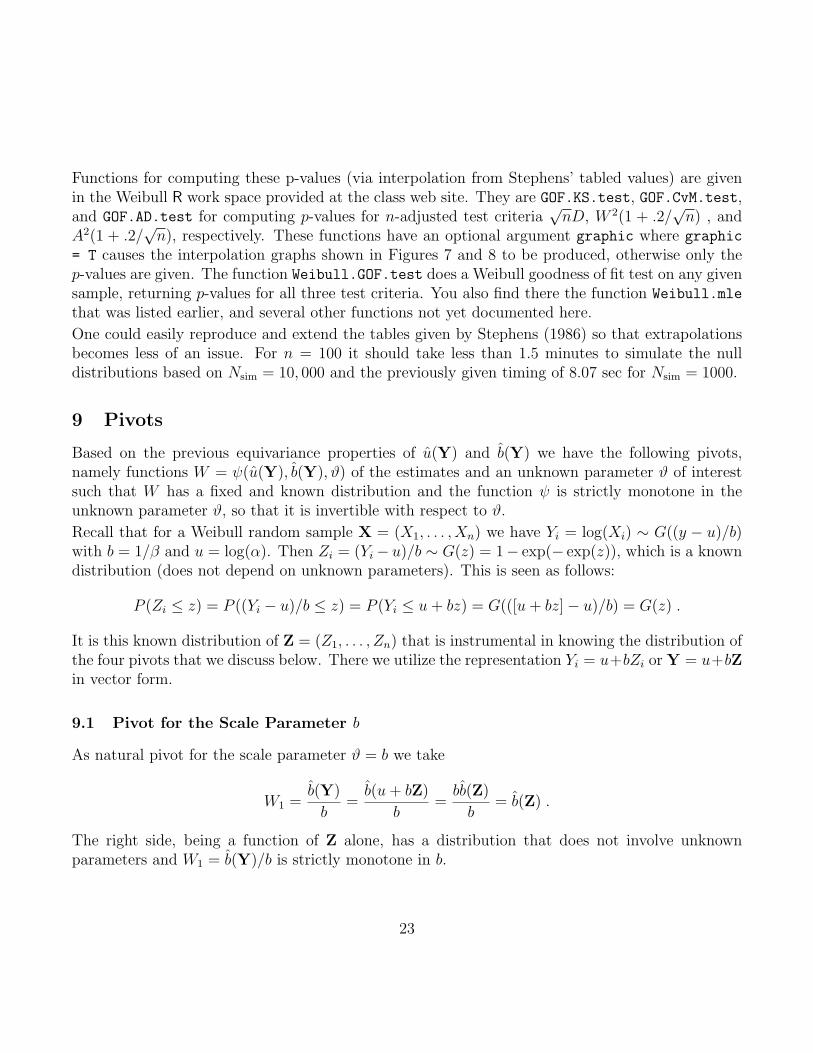
Functions for computing these p-values (via interpolation from Stephens’ tabled values) are givenin the Weibull R work space provided at the class web site. They are GOF.KS.test, GOF.CvM.test,and GOF.AD.test for computing p-values for n-adjusted test criteria
√nD, W 2(1 + .2/
√n) , and
A2(1 + .2/√n), respectively. These functions have an optional argument graphic where graphic
= T causes the interpolation graphs shown in Figures 7 and 8 to be produced, otherwise only thep-values are given. The function Weibull.GOF.test does a Weibull goodness of fit test on any givensample, returning p-values for all three test criteria. You also find there the function Weibull.mle
that was listed earlier, and several other functions not yet documented here.
One could easily reproduce and extend the tables given by Stephens (1986) so that extrapolationsbecomes less of an issue. For n = 100 it should take less than 1.5 minutes to simulate the nulldistributions based on Nsim = 10, 000 and the previously given timing of 8.07 sec for Nsim = 1000.
9 Pivots
Based on the previous equivariance properties of u(Y) and b(Y) we have the following pivots,namely functions W = ψ(u(Y), b(Y), ϑ) of the estimates and an unknown parameter ϑ of interestsuch that W has a fixed and known distribution and the function ψ is strictly monotone in theunknown parameter ϑ, so that it is invertible with respect to ϑ.
Recall that for a Weibull random sample X = (X1, . . . , Xn) we have Yi = log(Xi) ∼ G((y − u)/b)with b = 1/β and u = log(α). Then Zi = (Yi− u)/b ∼ G(z) = 1− exp(− exp(z)), which is a knowndistribution (does not depend on unknown parameters). This is seen as follows:
P (Zi ≤ z) = P ((Yi − u)/b ≤ z) = P (Yi ≤ u+ bz) = G(([u+ bz]− u)/b) = G(z) .
It is this known distribution of Z = (Z1, . . . , Zn) that is instrumental in knowing the distribution ofthe four pivots that we discuss below. There we utilize the representation Yi = u+bZi or Y = u+bZin vector form.
9.1 Pivot for the Scale Parameter b
As natural pivot for the scale parameter ϑ = b we take
W1 =b(Y)
b=b(u+ bZ)
b=bb(Z)
b= b(Z) .
The right side, being a function of Z alone, has a distribution that does not involve unknownparameters and W1 = b(Y)/b is strictly monotone in b.
23
●
●
●
●
●
A2 ×× ((1 ++ 0.2 n))
tail
prob
abili
ty p
on
log((
p((1
−−p))
)) sc
ale
0.0 0.5 1.0 1.5
0.00
10.
010.
050.
250.
50.
750.
9●
●
●
●
●
●
●
tabled valuesinterpolated/extrapolated values
●
●
●
●
●
W2 ×× ((1 ++ 0.2 n))
tail
prob
abili
ty p
on
log((
p((1
−−p))
)) sc
ale
0.00 0.05 0.10 0.15 0.20 0.25 0.30
0.00
10.
010.
050.
250.
50.
750.
9
●
●
●
●
●
●
●
tabled valuesinterpolated/extrapolated values
Figure 7: Interpolation & Extrapolation for A2(1 + .2/√n) and W 2(1 + .2/
√n)
24

●
●●
●
quadratic interpolation & linear extrapolation in 1 n
n (on 1 n scale)
∞∞ 500 200 100 50 40 30 25 20 15 10 9 8 7 6 5 4
0.80
30.
874
0.93
91.
007
n××
D−
quan
tile
D0.
9D
0.95
D0.
975
D0.
99
●
●●
●
●
●●
●●
●
●
● ●
●
●
● ●
●
tabled valuesinterpolated/extrapolated values
●
●
●
●
●
●
●
●
cubic interpolation & linear extrapolation in D
n ×× D
0.70 0.75 0.80 0.85 0.90 0.95 1.00 1.05
tail
prob
abili
ty p
on
log((
p((1
−−p))
)) sc
ale
0.00
10.
005
0.02
50.
10.
2
●
●
●
●
●
●
●
●
●
●
●
●
●
●
●
●
●
●
●
●
●
●
●
tabled valuesinterpolated quantilesinterpolated/extrapolated values
●
●
●
●
●
●
Figure 8: Interpolation & Extrapolation for√n×D
25
How do we obtain the distribution of b(Z)? An analytical approach does not seem possible. Theapproach followed here is that presented in Bain (1978), Bain and Engelhardt (1991) and originallyin Thoman et al. (1969, 1970), who provided tables for this distribution (and for those of the otherpivots discussed here) based on Nsim simulated values of b(Z) (and u(Z)), where Nsim = 20000 forn = 5, Nsim = 10000 for n = 6, 8, 10, 15, 20, 30, 40, 50, 75, and Nsim = 6000 for n = 100.
In these simulations one simply generates samples Z? = (Z1, . . . , Zn) ∼ G(z) and finds b(Z?) (andu(Z?) for the other pivots discussed later) for each such sample Z?. By simulating this processNsim = 10000 times we obtain b(Z?
1), . . . , b(Z?Nsim
). The empirical distribution function of these
simulated estimates b(Z?i ), denoted by H1(w), provides a fairly reasonable estimate of the sampling
distribution H1(w) of b(Z) and thus also of the pivot distribution of W1 = b(Y)/b. From thissimulated distribution we can estimate any γ-quantile of H1(w) to any practical accuracy, providedNsim is sufficiently large. Values of γ closer to 0 or 1 require higher Nsim. For .005 ≤ γ ≤ .995 asimulation level of Nsim = 10000 should be quite adequate.
If we denote the γ-quantile of H1(w) by η1(γ), i.e.,
γ = H1(η1(γ)) = P (b(Y)/b ≤ η1(γ)) = P (b(Y)/η1(γ) ≤ b)
we see that b(Y)/η1(γ) can be viewed as a 100γ% lower bound to the unknown parameter b. We donot know η1(γ) but we can estimate it by the corresponding quantile η1(γ) of the simulated distri-bution H1(w) which serves as proxy for H1(w). We then use b(Y)/η1(γ) as an approximate 100γ%lower bound to the unknown parameter b. For large Nsim, say Nsim = 10000, this approximation ispractically quite adequate.
We note here that a 100γ% lower bound can be viewed as a 100(1 − γ)% upper bound, because1 − γ is the chance of the lower bound falling on the wrong side of its target, namely above. Toget 100γ% upper bounds one simply constructs 100(1 − γ)% lower bounds by the above method.Similar comments apply to the pivots obtained below, where we only give one-sided bounds (loweror upper) in each case.
Based on the relationship b = 1/β the respective 100γ% approximate lower and upper confidencebounds for the Weibull shape parameter would be
η1(1− γ)
b(Y)= η1(1− γ)× β(X) and
η1(γ)
b(Y)= η1(γ)× β(X)
and an approximate 100γ% confidence interval for β would be[η1((1− γ)/2)× β(X), η1((1 + γ)/2)× β(X)
]since (1 + γ)/2 = 1− (1− γ)/2. Here X = (X1, . . . , Xn) is the untransformed Weibull sample.
26
9.2 Pivot for the Location Parameter u
For the location parameter ϑ = u we have the following pivot
W2 =u(Y)− u
b(Y)=u(u+ bZ)− u
b(u+ bZ)=u+ bu(Z)− u
bb(Z)=u(Z)
b(Z).
It has a distribution that does not depend on any unknown parameter, since it only depends on theknown distribution of Z. Furthermore W2 is strictly decreasing in u. Thus W2 is a pivot with respectto u. Denote this pivot distribution of W2 by H2(w) and its γ-quantile by η2(γ). As before thispivot distribution and its quantiles can be approximated sufficiently well by simulating u(Z?)/b(Z?)a sufficient number Nsim times and using the empirical cdf H2(w) of the u(Z?
i )/b(Z?i ) as proxy for
H2(w).
As in the previous pivot case we can exploit this pivot distribution as follows
γ = H2(η2(γ)) = P
(u(Y)− u
b(Y)≤ η2(γ)
)= P (u(Y)− b(Y)η2(γ) ≤ u)
and thus we can view u(Y) − b(Y)η2(γ) as a 100γ% lower bound for the unknown parameter u.Using the γ-quantile η2(γ) obtained from the empirical cdf H2(w) we then treat u(Y)− b(Y)η2(γ)as an approximate 100γ% lower bound for the unknown parameter u.
Based on the relation u = log(α) this translates into an approximate 100γ% lower bound
exp(u(Y)− b(Y)η2(γ)) = exp(log(α(X))− η2(γ)/β(X)) = α(X) exp(−η2(γ)/β(X)) for α.
Upper bounds and intervals are handled as in the previous situation for b or β.
9.3 Pivot for the p-quantile yp
With respect to the p-quantile ϑ = yp = u+ b log(− log(1− p)) = u+ bwp of the Y distribution thenatural pivot is
Wp =yp(Y)− yp
b(Y)=
u(Y) + b(Y)wp − (u+ bwp)
b(Y)=u(u+ bZ) + b(u+ bZ)wp − (u+ bwp)
b(u+ bZ)
=u+ bu(Z) + bb(Z)wp − (u+ bwp)
bb(Z)=u(Z) + (b(Z)− 1)wp
b(Z).
Again its distribution only depends on the known distribution of Z and not on the unknown param-eters u and b and the pivot Wp is a strictly decreasing function of yp. Denote this pivot distribution
27
function by Hp(w) and its γ-quantile by ηp(γ). As before, this pivot distribution and its quantiles
can be approximated sufficiently well by simulating{u(Z) + (b(Z)− 1)wp
}/b(Z) a sufficient num-
ber Nsim times. Denote the empirical cdf of such simulated values by Hp(w) and the correspondingγ-quantiles by ηp(γ).
As before we proceed with
γ = Hp(ηp(γ)) = P
(yp(Y)− yp
b(Y)≤ ηp(γ)
)= P
(yp(Y)− ηp(γ)b(Y) ≤ yp
)
and thus we can treat yp(Y) − ηp(γ)b(Y) as a 100γ% lower bound for yp. Again we can treat
yp(Y)− ηp(γ)b(Y) as an approximate 100γ% lower bound for yp.
Sinceyp(Y)− ηp(γ)b(Y) = u(Y) + wpb(Y)− ηp(γ)b(Y) = u(Y)− kp(γ)b(Y)
with kp(γ) = ηp(γ)− wp, we could have obtained the same lower bound by the following argumentthat does not use a direct pivot, namely
γ = P (u(Y)− kp(γ)b(Y) ≤ yp) = P (u(Y)− kp(γ)b(Y) ≤ u+ bwp)
= P (u(Y)− u− kp(γ)b(Y) ≤ bwp)
= P
(u(Y)− u
b− kp(γ)
b(Y)
b≤ wp
)
= P (u(Z)− kp(γ)b(Z) ≤ wp) = P
(u(Z)− wp
b(Z)≤ kp(γ)
)
and we see that kp(γ) can be taken as the γ-quantile of the distribution of (u(Z)− wp)/b(Z).
This distribution can be estimated by the empirical cdf of Nsim simulated values (u(Z?i )−wp)/b(Z
?i ),
i = 1, . . . , Nsim and its γ-quantile kp(γ) serves as a good approximation to kp(γ).
It is easily seen that this produces the same quantile lower bound as before. However, in thisapproach one sees one further detail, namely that h(p) = −kp(γ) is strictly increasing in p1, sincewp is strictly increasing in p.
1Suppose p1 < p2 and h(p1) ≥ h(p2) with γ = P (u(Z) + h(p1)b(Z) ≤ wp1) and γ = P (u(Z) + h(p2)b(Z) ≤ wp2) =P (u(Z) + h(p1)b(Z) ≤ wp1 + (wp2 − wp1) + (h(p1) − h(p2))b(Z)) ≥ P (u(Z) + h(p1)b(Z) ≤ wp1 + (wp2 − wp1)) > γ
(i.e., γ > γ, a contradiction) since P (wp1 < u(Z)+h(p1)b(Z) ≤ wp1 +(wp2 −wp1)) > 0. A thorough argument wouldshow that b(z) and thus u(z) are continuous functions of z = (z1, . . . , zn) and since there is positive probability inany neighborhood of any z ∈ R there is positive probability in any neighborhood of (u(z), b(z)).
28
Of course it makes intuitive sense that quantile lower bounds should be increasing in p since itstarget p-quantiles are increasing in p. This strictly increasing property allows us to immediatelyconstruct upper confidence bounds for left tail probabilities as is shown in the next section.
Since xp = exp(yp) is the corresponding p-quantile of the Weibull distribution we can view
exp(yp(Y)− ηp(γ)b(Y)
)= α(X) exp
((wp − ηp(γ))/β(X)
)= α(X) exp
(−kp(γ)/β(X)
)as an approximate 100γ% lower bound for xp = exp(u+ bwp) = α(− log(1− p))1/β.
Since α is the (1 − exp(−1))-quantile of the Weibull distribution, lower bounds for it can be seenas a special case of quantile lower bounds. Indeed, this particular quantile lower bound coincideswith the one given previously.
9.4 Upper Confidence Bounds for the Tail Probability p(y) = P (Y ≤ y)
As far as an appropriate pivot for p(y) = P (Y ≤ y) is concerned, the situation here is not asstraightforward as in the previous three cases. Clearly
p(y) = G
(y − u(Y)
b(Y)
)is the natural estimate (mle) of p(y) = P (Y ≤ y) = G
(y − u
b
)
and one easily sees that the distribution function H of this estimate depends on u and b onlythrough p(y), namely
p(y) = G
(y − u(Y)
b(Y)
)= G
((y − u)/b− (u(Y)− u)/b
b(Y)/b
)= G
(G−1(p(y))− u(Z)
b(Z)
)∼ Hp(y) .
Thus by the probability integral transform it follows that
Wp(y) = Hp(y) (p(y)) ∼ U(0, 1)
i.e., Wp(y) is a true pivot, contrary to what is stated in Bain (1978) and Bain and Engelhardt (1991).
Rather than using this pivot we will go a more direct route as was indicated by the strictly increasingproperty of h(p) = hγ(p) in the previous section. Denote by h−1(·) the inverse function to h(·). Wethen have
γ = P (u(Y)+h(p)b(Y) ≤ yp) = P (h(p) ≤ (yp− u(Y))/b(Y)) = P(p ≤ h−1
((yp − u(Y))/b(Y)
)),
for any p ∈ (0, 1). If we parameterize such p via p(y) = P (Y ≤ y) = G((y− u)/b) we have yp(y) = yand thus also
γ = P(p(y) ≤ h−1
((y − u(Y))/b(Y)
))29
for any y ∈ R and u ∈ R and b > 0. Hence pU(y) = h−1((y − u(Y))/b(Y)
)can be viewed as
100γ% upper confidence bound for p(y) for any given threshold y.
The only remaining issue is the computation of such bounds. Does it require the inversion of hand the concomitant calculations of many h(p) = −k(p) for the iterative convergence of such aninversion? It turns out that there is a direct path just as we had it in the previous three confidencebound situations.
Note that h−1(x) solves −kp = x for p. We claim that h−1(x) is the γ-quantile of the G(u(Z)+xb(Z))
distribution which we can simulate by calculating as before u(Z) and b(Z) a large numberNsim times.The above claim concerning h−1(x) is seen as follows. If for any x = h(p) we have
P (G(u(Z) + xb(Z)) ≤ h−1(x)) = P (G(u(Z) + h(p)b(Z)) ≤ p)
= P (u(Z) + h(p)b(Z) ≤ wp)
= P (u(Z)− kγ(p)b(Z) ≤ wp) = γ ,
as seen in the previous section. Thus h−1(x) is the γ-quantile of the G(u(Z) + xb(Z)) distribution.
If we observe Y = y and obtain u(y) and b(y) as our maximum likelihood estimates for u andb we get our 100γ% upper bound for p(y) = G((y − u)/b) as follows: For the fixed value ofx = (y − u(y))/b(y) = G−1(p(y)) simulate the G(u(Z) + xb(Z)) distribution (with sufficiently highNsim) and calculate the γ-quantile of this distribution as the desired approximate 100γ% upperbound for p(y) = P (Y ≤ y) = G((y − u)/b).
10 Tabulation of Confidence Quantiles η(γ)
For the pivots for b, u and yp it is possible to carry out simulations once and for all for a desired setof confidence levels γ, sample sizes n and choices of p, and tabulate the required confidence quantilesη1(γ), η2(γ), and ηp(γ). This has essentially been done (with
√n scaling modifications) and such
tables are given in Bain (1978), Bain and Engelhardt (1991) and Thoman et al. (1969,1970). Similartables for bounds on p(y) are not quite possible since the appropriate bounds depend on the observedvalue of p(y), which varies from sample to sample. Instead Bain (1978), Bain and Engelhardt (1991)and Thoman et al. (1970) tabulate confidence bounds for p(y) for a reasonably fine grid of valuesfor p(y), which can then serve for interpolation purposes with the actually observed value of p(y).
It should be quite clear that all this requires extensive tabulation. The use of these tables is noteasy. Table 4 in Bain (1978) does not have a consistent format and using these tables wouldrequire delving deeply into the text for each new use, unless one does this kind of calculation allthe time. In fact, in the second edition, Bain and Engelhardt (1991), Table 4 has been greatlyreduced to just cover the confidence factors dealing with the location parameter u, and it now
30
leaves out the confidence factors for general p-quantiles. For the p-quantiles one is referred to thesame interpolation scheme that is needed when getting confidence bounds for p(y), using Table 7in Bain and Engelhardt (1991). The example that they present (page 248) would have benefittedby showing some intermediate steps in the interpolation process. They point out that the resultingconfidence bound for xp is slightly different (14.03) from that obtained using the confidence quantilesof the original Table 4, namely 13.92. They attribute the difference to round-off errors or otherdiscrepancies. Among the latter one may consider that possibly different simulations were involved.
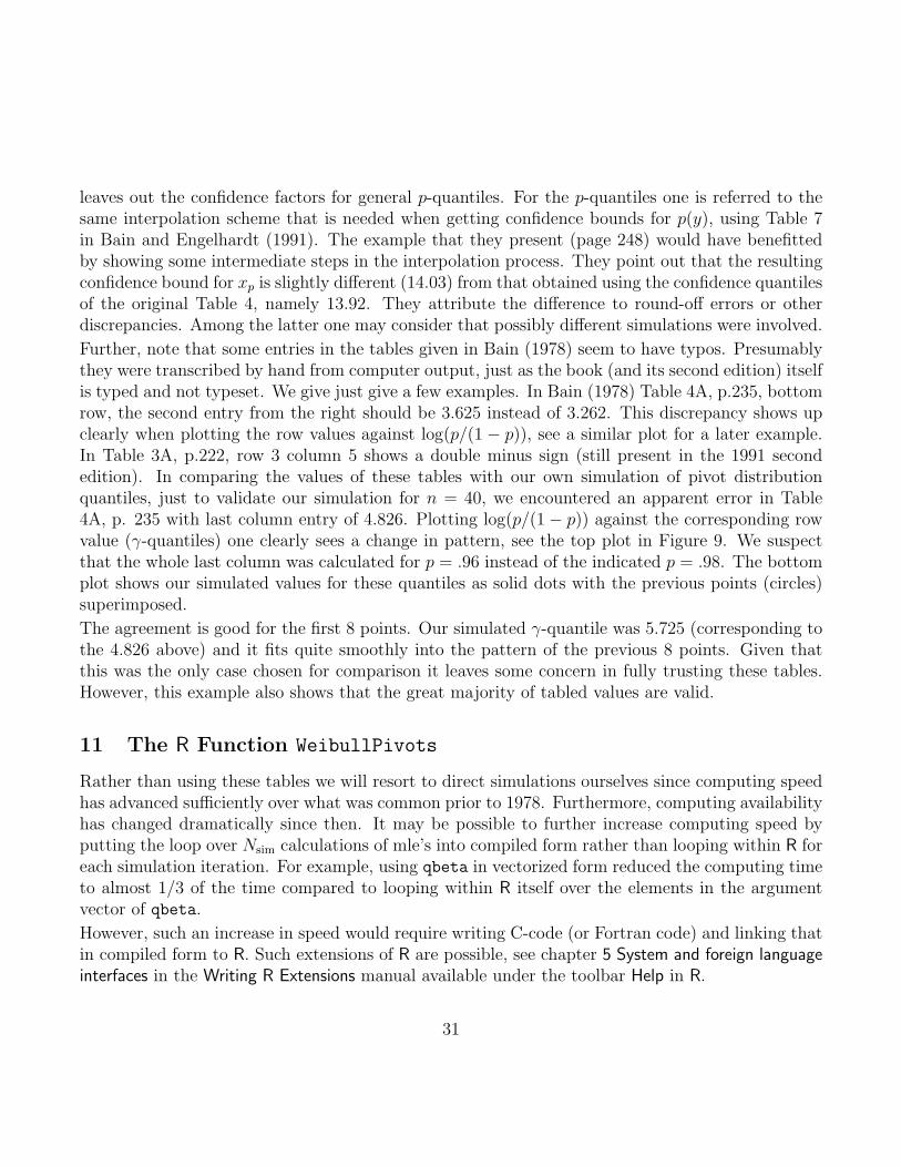
Further, note that some entries in the tables given in Bain (1978) seem to have typos. Presumablythey were transcribed by hand from computer output, just as the book (and its second edition) itselfis typed and not typeset. We give just give a few examples. In Bain (1978) Table 4A, p.235, bottomrow, the second entry from the right should be 3.625 instead of 3.262. This discrepancy shows upclearly when plotting the row values against log(p/(1 − p)), see a similar plot for a later example.In Table 3A, p.222, row 3 column 5 shows a double minus sign (still present in the 1991 secondedition). In comparing the values of these tables with our own simulation of pivot distributionquantiles, just to validate our simulation for n = 40, we encountered an apparent error in Table4A, p. 235 with last column entry of 4.826. Plotting log(p/(1− p)) against the corresponding rowvalue (γ-quantiles) one clearly sees a change in pattern, see the top plot in Figure 9. We suspectthat the whole last column was calculated for p = .96 instead of the indicated p = .98. The bottomplot shows our simulated values for these quantiles as solid dots with the previous points (circles)superimposed.
The agreement is good for the first 8 points. Our simulated γ-quantile was 5.725 (corresponding tothe 4.826 above) and it fits quite smoothly into the pattern of the previous 8 points. Given thatthis was the only case chosen for comparison it leaves some concern in fully trusting these tables.However, this example also shows that the great majority of tabled values are valid.
11 The R Function WeibullPivots
Rather than using these tables we will resort to direct simulations ourselves since computing speedhas advanced sufficiently over what was common prior to 1978. Furthermore, computing availabilityhas changed dramatically since then. It may be possible to further increase computing speed byputting the loop over Nsim calculations of mle’s into compiled form rather than looping within R foreach simulation iteration. For example, using qbeta in vectorized form reduced the computing timeto almost 1/3 of the time compared to looping within R itself over the elements in the argumentvector of qbeta.
However, such an increase in speed would require writing C-code (or Fortran code) and linking thatin compiled form to R. Such extensions of R are possible, see chapter 5 System and foreign languageinterfaces in the Writing R Extensions manual available under the toolbar Help in R.
31
●
●
●●
●
●
●
●
●
2 3 4 5
01
23
4
Bain's tabled quantiles for n=40, γγ == 0.9
log(
p/(1
− p
))
●0.96
0.98
●
●
●●
●
●
●
●
●
2 3 4 5
01
23
4
our simulated quantiles for n=40, γγ == 0.9
log(
p/(1
− p
))
●
●
●●
●
●
●
●
●
Figure 9: Abnormal Behavior of Tabulated Confidence Quantiles
32

For the R function WeibullPivots (available within the R work space for Weibull DistributionApplications on the class web site) the call
system.time(WeibullPivots(Nsim = 10000, n = 10, r = 10, graphics = F))
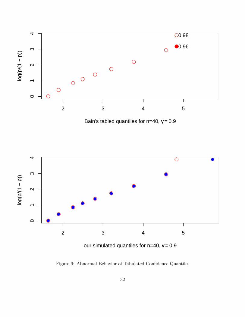
gave an elapsed time of 59.76 seconds. Here the default sample size n = 10 was used and r = 10(also default) indicates that the 10 lowest sample values are given and used, i.e., in this case thefull sample. Also, an internally generated Weibull data set was used, since the default in the call toWeibullPivots is weib.sample=NULL. For sample sizes n = 100 with r = 100 and n = 1000 withr = 1000 the corresponding calls resulted in elapsed times of 78.22 and 269.32 seconds, respectively.These three computing times suggest strong linear behavior in n as is illustrated in Figure 10. Theintercept 57.35 and slope of .2119 given here are fairly consistent with the intercept .005886 andslope of 2.001× 10⁻⁵ given in Figure 4. The latter give the calculation time of a single set of mle’swhile in the former case we calculate Nsim = 10000 such mle’s, i.e., the previous slope and interceptfor a single mle calculation need to be scaled up by the factor 10000.
For all the previously discussed confidence bounds, be they upper or lower bounds for their respectivetargets, all that is needed is the set of (u(zi), b(zi)) for i = 1, . . . , Nsim. Thus we can constructconfidence bounds and intervals for u and b, for yp for any collection of p values, and for p(y) and1− p(y) for any collection of threshold values y and we can do this for any set of confidence levelsthat make sense for the simulated distributions, i.e., we don’t have to run the simulations over andover for each target parameter, confidence level, p or y, unless one wants independent simulationsfor some reason.
Proper use of this function only requires understanding the calling arguments, purpose, and outputof this function, and the time to run the simulations. The time for running the simulation shouldeasily beat the time spent in dealing with tabulated confidence quantiles in order to get desiredconfidence bounds, especially since WeibullPivots does such calculations all at once for a broadspectrum of yp and p(y) and several confidence levels without greatly impacting the computing time.Furthermore, WeibullPivots does all this not only for full samples but also for type II censoredsamples, for which appropriate confidence factors are available only sparsely in tables.
We will now explain the calling sequence of WeibullPivots and its output. The calling sequencewith all arguments given with their default values is as follows:
WeibullPivots(weib.sample=NULL,alpha=10000,beta=1.5,n=10,r=10,
Nsim=1000,threshold=NULL,graphics=T)
Here Nsim = Nsim has default value 1000 which is appropriate when trying to get a feel for thefunction for any particular data set. The sample size is input as n = n and r = r indicates thenumber of smallest sample values available for analysis. When r < n we are dealing with a type IIcensored data set where observation stops as soon as the smallest r lifetimes have been observed.
We need r > 1 and at least two distinct observations among X(1), . . . , X(r) in order to estimate
33
●
●
●
0 200 400 600 800 1000
050
100
150
200
250
300
sample size n
elap
sed
time
for
Wei
bullP
ivot
s(N
sim
=10
000)
==
intercept slope
57.350.2119
Figure 10: Timings for WeibullPivots for Various n
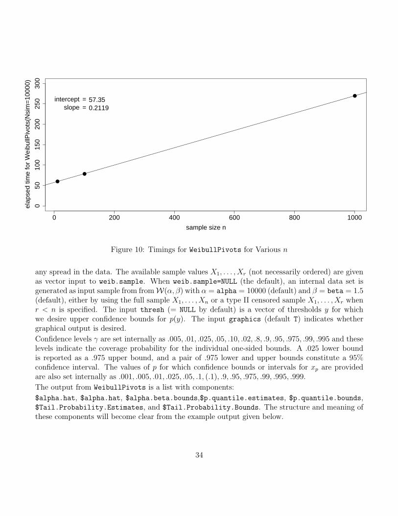
any spread in the data. The available sample values X1, . . . , Xr (not necessarily ordered) are givenas vector input to weib.sample. When weib.sample=NULL (the default), an internal data set isgenerated as input sample from fromW(α, β) with α = alpha = 10000 (default) and β = beta = 1.5(default), either by using the full sample X1, . . . , Xn or a type II censored sample X1, . . . , Xr whenr < n is specified. The input thresh (= NULL by default) is a vector of thresholds y for whichwe desire upper confidence bounds for p(y). The input graphics (default T) indicates whethergraphical output is desired.
Confidence levels γ are set internally as .005, .01, .025, .05, .10, .02, .8, .9, .95, .975, .99, .995 and theselevels indicate the coverage probability for the individual one-sided bounds. A .025 lower boundis reported as a .975 upper bound, and a pair of .975 lower and upper bounds constitute a 95%confidence interval. The values of p for which confidence bounds or intervals for xp are providedare also set internally as .001, .005, .01, .025, .05, .1, (.1), .9, .95, .975, .99, .995, .999.
The output from WeibullPivots is a list with components:
$alpha.hat, $alpha.hat, $alpha.beta.bounds,$p.quantile.estimates, $p.quantile.bounds,$Tail.Probability.Estimates, and $Tail.Probability.Bounds. The structure and meaning ofthese components will become clear from the example output given below.
34
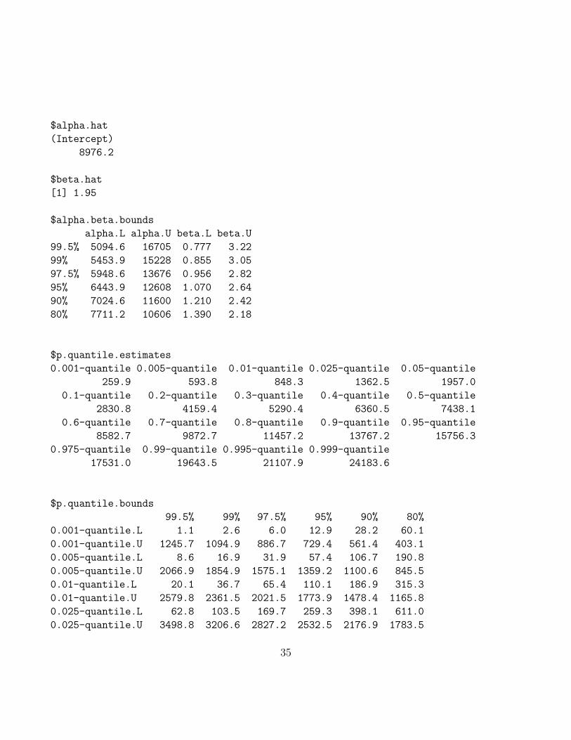
$alpha.hat
(Intercept)
8976.2
$beta.hat
[1] 1.95
$alpha.beta.bounds
alpha.L alpha.U beta.L beta.U
99.5% 5094.6 16705 0.777 3.22
99% 5453.9 15228 0.855 3.05
97.5% 5948.6 13676 0.956 2.82
95% 6443.9 12608 1.070 2.64
90% 7024.6 11600 1.210 2.42
80% 7711.2 10606 1.390 2.18
$p.quantile.estimates
0.001-quantile 0.005-quantile 0.01-quantile 0.025-quantile 0.05-quantile
259.9 593.8 848.3 1362.5 1957.0
0.1-quantile 0.2-quantile 0.3-quantile 0.4-quantile 0.5-quantile
2830.8 4159.4 5290.4 6360.5 7438.1
0.6-quantile 0.7-quantile 0.8-quantile 0.9-quantile 0.95-quantile
8582.7 9872.7 11457.2 13767.2 15756.3
0.975-quantile 0.99-quantile 0.995-quantile 0.999-quantile
17531.0 19643.5 21107.9 24183.6
$p.quantile.bounds
99.5% 99% 97.5% 95% 90% 80%
0.001-quantile.L 1.1 2.6 6.0 12.9 28.2 60.1
0.001-quantile.U 1245.7 1094.9 886.7 729.4 561.4 403.1
0.005-quantile.L 8.6 16.9 31.9 57.4 106.7 190.8
0.005-quantile.U 2066.9 1854.9 1575.1 1359.2 1100.6 845.5
0.01-quantile.L 20.1 36.7 65.4 110.1 186.9 315.3
0.01-quantile.U 2579.8 2361.5 2021.5 1773.9 1478.4 1165.8
0.025-quantile.L 62.8 103.5 169.7 259.3 398.1 611.0
0.025-quantile.U 3498.8 3206.6 2827.2 2532.5 2176.9 1783.5
35
0.05-quantile.L 159.2 229.2 352.6 497.5 700.0 1011.9
0.05-quantile.U 4415.7 4081.3 3673.7 3329.5 2930.0 2477.2
0.1-quantile.L 398.3 506.3 717.4 962.2 1249.5 1679.1
0.1-quantile.U 5584.6 5261.9 4811.6 4435.7 3990.8 3474.1
0.2-quantile.L 1012.6 1160.2 1518.8 1882.9 2287.1 2833.2
0.2-quantile.U 7417.1 6978.2 6492.8 6031.2 5543.2 4946.9
0.3-quantile.L 1725.4 1945.2 2383.9 2820.0 3305.0 3929.0
0.3-quantile.U 8919.8 8460.0 7939.8 7384.1 6865.0 6211.4
0.4-quantile.L 2548.0 2848.2 3345.2 3806.6 4353.9 5008.2
0.4-quantile.U 10616.3 10130.4 9380.3 8778.2 8139.3 7421.2
0.5-quantile.L 3502.4 3881.1 4415.1 4873.3 5443.0 6107.3
0.5-quantile.U 12809.0 11919.1 10992.9 10226.8 9485.1 8703.4
0.6-quantile.L 4694.0 5022.6 5573.8 6052.8 6624.4 7300.4
0.6-quantile.U 15626.1 14350.6 12941.3 11974.8 11041.1 10106.2
0.7-quantile.L 6017.1 6399.0 6876.6 7345.8 7938.2 8628.0
0.7-quantile.U 19271.6 17679.9 15545.8 14181.1 12958.0 11784.2
0.8-quantile.L 7601.3 7971.0 8465.4 8933.5 9504.0 10244.2
0.8-quantile.U 24765.2 22445.0 19286.0 17236.0 15605.6 13952.2
0.9-quantile.L 9674.7 10033.7 10538.6 11031.1 11653.0 12460.3
0.9-quantile.U 35233.4 31065.3 26037.4 22670.5 19835.3 17417.5
0.95-quantile.L 11203.6 11584.6 12145.2 12660.2 13365.5 14311.2
0.95-quantile.U 46832.9 40053.3 32863.1 27904.7 23903.9 20703.0
0.975-quantile.L 12434.7 12833.5 13449.7 14030.5 14781.8 15909.1
0.975-quantile.U 59783.1 49209.9 39397.8 33118.7 27938.4 23773.7
0.99-quantile.L 13732.6 14207.7 14876.0 15530.0 16431.7 17783.1
0.99-quantile.U 76425.0 61385.4 48625.4 40067.3 33233.8 27729.8
0.995-quantile.L 14580.4 15115.4 15810.0 16530.6 17551.8 19081.0
0.995-quantile.U 89690.9 71480.4 55033.4 45187.1 36918.7 30505.0
0.999-quantile.L 16377.7 16885.9 17642.5 18557.1 19792.4 21744.7
0.999-quantile.U 121177.7 95515.7 71256.5 56445.5 45328.1 36739.2
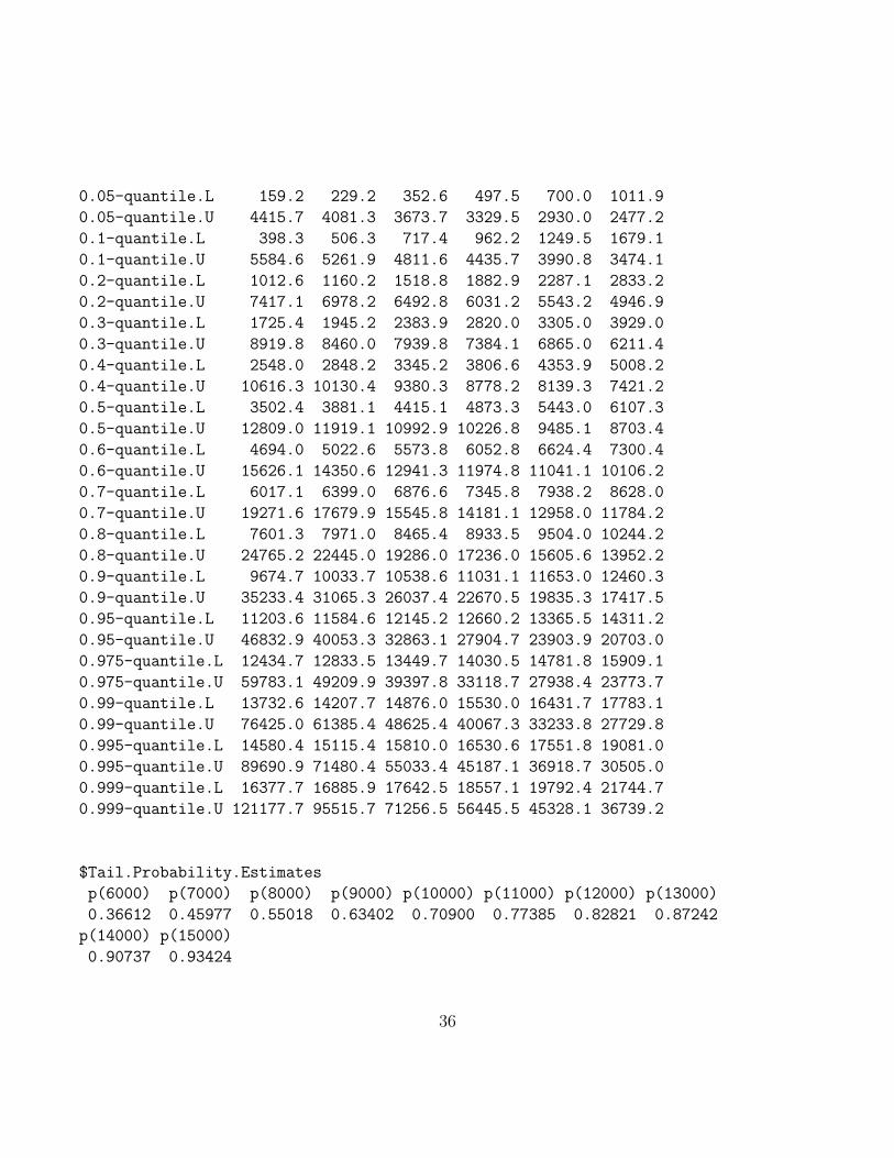
$Tail.Probability.Estimates
p(6000) p(7000) p(8000) p(9000) p(10000) p(11000) p(12000) p(13000)
0.36612 0.45977 0.55018 0.63402 0.70900 0.77385 0.82821 0.87242
p(14000) p(15000)
0.90737 0.93424
36
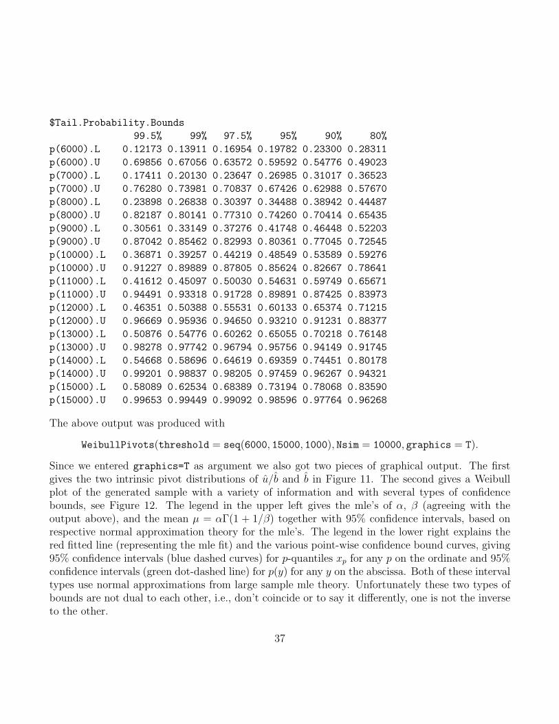
$Tail.Probability.Bounds
99.5% 99% 97.5% 95% 90% 80%
p(6000).L 0.12173 0.13911 0.16954 0.19782 0.23300 0.28311
p(6000).U 0.69856 0.67056 0.63572 0.59592 0.54776 0.49023
p(7000).L 0.17411 0.20130 0.23647 0.26985 0.31017 0.36523
p(7000).U 0.76280 0.73981 0.70837 0.67426 0.62988 0.57670
p(8000).L 0.23898 0.26838 0.30397 0.34488 0.38942 0.44487
p(8000).U 0.82187 0.80141 0.77310 0.74260 0.70414 0.65435
p(9000).L 0.30561 0.33149 0.37276 0.41748 0.46448 0.52203
p(9000).U 0.87042 0.85462 0.82993 0.80361 0.77045 0.72545
p(10000).L 0.36871 0.39257 0.44219 0.48549 0.53589 0.59276
p(10000).U 0.91227 0.89889 0.87805 0.85624 0.82667 0.78641
p(11000).L 0.41612 0.45097 0.50030 0.54631 0.59749 0.65671
p(11000).U 0.94491 0.93318 0.91728 0.89891 0.87425 0.83973
p(12000).L 0.46351 0.50388 0.55531 0.60133 0.65374 0.71215
p(12000).U 0.96669 0.95936 0.94650 0.93210 0.91231 0.88377
p(13000).L 0.50876 0.54776 0.60262 0.65055 0.70218 0.76148
p(13000).U 0.98278 0.97742 0.96794 0.95756 0.94149 0.91745
p(14000).L 0.54668 0.58696 0.64619 0.69359 0.74451 0.80178
p(14000).U 0.99201 0.98837 0.98205 0.97459 0.96267 0.94321
p(15000).L 0.58089 0.62534 0.68389 0.73194 0.78068 0.83590
p(15000).U 0.99653 0.99449 0.99092 0.98596 0.97764 0.96268
The above output was produced with
WeibullPivots(threshold = seq(6000, 15000, 1000), Nsim = 10000, graphics = T).
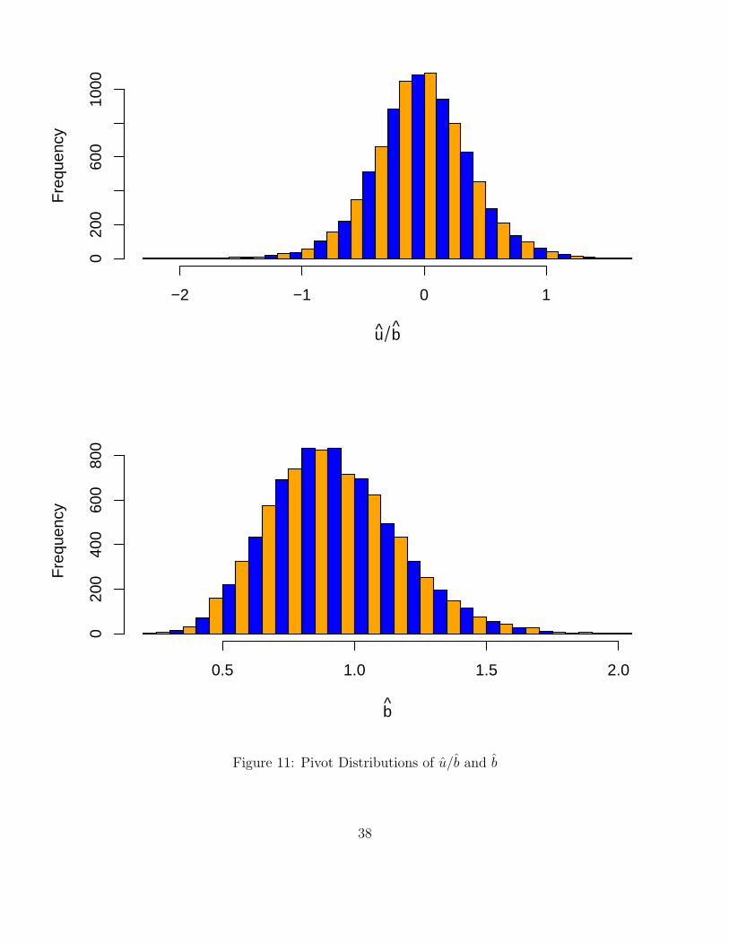
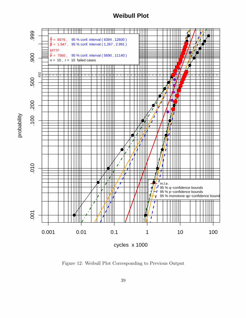
Since we entered graphics=T as argument we also got two pieces of graphical output. The firstgives the two intrinsic pivot distributions of u/b and b in Figure 11. The second gives a Weibullplot of the generated sample with a variety of information and with several types of confidencebounds, see Figure 12. The legend in the upper left gives the mle’s of α, β (agreeing with theoutput above), and the mean µ = αΓ(1 + 1/β) together with 95% confidence intervals, based onrespective normal approximation theory for the mle’s. The legend in the lower right explains thered fitted line (representing the mle fit) and the various point-wise confidence bound curves, giving95% confidence intervals (blue dashed curves) for p-quantiles xp for any p on the ordinate and 95%confidence intervals (green dot-dashed line) for p(y) for any y on the abscissa. Both of these intervaltypes use normal approximations from large sample mle theory. Unfortunately these two types ofbounds are not dual to each other, i.e., don’t coincide or to say it differently, one is not the inverseto the other.
37
u b
Fre
quen
cy
−2 −1 0 1
020
060
010
00
b
Fre
quen
cy
0.5 1.0 1.5 2.0
020
040
060
080
0
Figure 11: Pivot Distributions of u/b and b
38
cycles x 1000
prob
abili
ty
●
●
●
●
●
●
●
●
●
●
0.001 0.01 0.1 1 10 100
.001
.010
.100
.200
.500
.900
.999
.632
m.l.e.95 % q−confidence bounds95 % p−confidence bounds95 % monotone qp−confidence bounds
Weibull Plot
αα = 8976 , 95 % conf. interval ( 6394 , 12600 )ββ = 1.947 , 95 % conf. interval ( 1.267 , 2.991 )
MTTFµµ = 7960 , 95 % conf. interval ( 5690 , 11140 )n = 10 , r = 10 failed cases
●
●
●
●
●
●
●
●
●
●
●
●
●
●
●
●
●●
●
●
●
●
●
●
●
●
●
●
●
●
●
●
●
●
●
●●
●
●
●●●●●●●●●●
●●●●●●●●●
Figure 12: Weibull Plot Corresponding to Previous Output
39
A third type of bound is presented in the orange curve which simultaneously provides 95% confidenceintervals for xp and p(x), depending on the direction in which the curves are used. We either readsideways from p and down from the curve (at that p level) to get upper and lower bounds for xp, orwe read vertically up from an abscissa value x to read off upper and lower bounds for p(x) on theordinate axis as we go from the respective curves at that x value to the left. These latter boundsare also based on normal mle approximation theory and the approximation will naturally suffer forsmall sample sizes. However, the principle behind these bounds is a unifying one in that the samecurve is used for quantile and tail probability bounds. If instead of using the approximating normaldistribution one uses the parametric bootstrap approach (simulating samples from an estimatedWeibull distribution) the unifying principle reduces to the pivot simulation approach, i.e., is basicallyexact except for the simulation aspect Nsim <∞.
The curves representing the latter (pivots with simulated distributions) are the solid black linesconnecting the solid black dots which represent the xp 95% confidence intervals (using the 97.5%lower and upper bounds to xp given in our output example above. Also seen on these curves aresolid red dots that correspond to the abscissa values x = 6000, (1000), 15000 and viewed verticallythey represent 95% confidence intervals for p(x). This illustrates that the same curves are used.
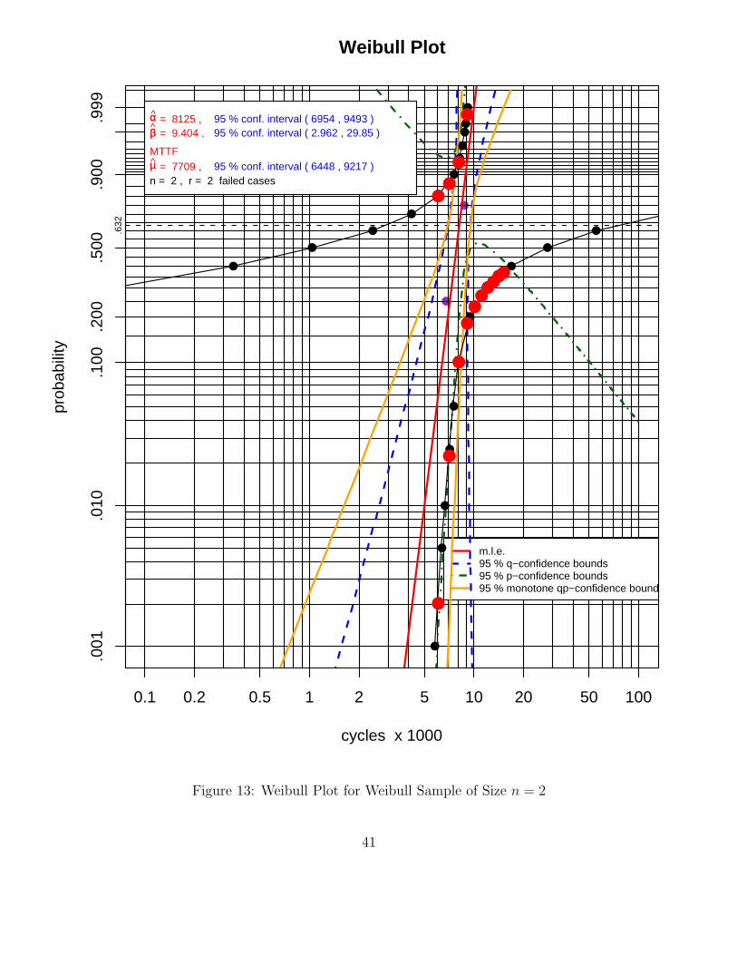
Figure 13 represents an extreme case where we have a sample of size n = 2 and here another aspectbecomes apparent. Both of the first two types of bounds (blue and green) are no longer monotonein p or x respectively. This is in the nature of an imperfect normal approximation for these twoapproaches. Thus we could not (at least not generally) have taken either to take the role of servingboth purposes, i.e., as providing bounds for xp and p(x) simultaneously. However, the orange curveis still monotone and still serves that dual purpose, although its coverage probability properties arebound to be affected badly by the small sample size n = 2. The pivot based curves are also strictlymonotone and they have exact coverage probability, subject to the Nsim <∞ limitation.
40
cycles x 1000
prob
abili
ty
●
●
0.1 0.2 0.5 1 2 5 10 20 50 100
.001
.010
.100
.200
.500
.900
.999
.632
m.l.e.95 % q−confidence bounds95 % p−confidence bounds95 % monotone qp−confidence bounds
Weibull Plot
αα = 8125 , 95 % conf. interval ( 6954 , 9493 )ββ = 9.404 , 95 % conf. interval ( 2.962 , 29.85 )
MTTFµµ = 7709 , 95 % conf. interval ( 6448 , 9217 )n = 2 , r = 2 failed cases
●
●
●
●
●
●
●
●
●
●
●
●
●
●
●
●
●
●
●
●
●
●●
●
●
●
●
●●●●●
●●
●●
●
●
●
Figure 13: Weibull Plot for Weibull Sample of Size n = 2
41
12 Regression
Here we extend the results of the previous location/scale model for log-transformed Weibull samplesto the more general regression model where the location parameter u for Yi = log(Xi) can vary withi, specifically it varies as a linear combination of known covariates ci,1, . . . , ci,k for the ith observationas follows:
ui = ζ1ci,1 + . . .+ ζkci,k , i = 1, . . . , n ,
while the scale parameter b stays constant. Thus we have the following model for Y1, . . . , Yn
Yi = ui + bEi = ζ1ci,1 + . . .+ ζkci,k + bZi , i = 1, . . . , n ,
with independent Zi ∼ G(z) = 1− exp(− exp(z)), i = 1, . . . , n, and unknown parameters b > 0 andζ1, . . . , ζk ∈ R.
Two concrete examples of this general linear model will be discussed in detail later on. The first isthe simple linear regression model and the other is the k-sample model, which exemplifies ANOVAsituations.
It can be shown (Scholz, 1996) that the mle’s ζ ′ = (ζ1, . . . , ζk) and b of ζ and b exist and are uniqueprovided the covariate matrix C, consisting of the rows c′i = (ci,1, . . . , ci,k), i = 1, . . . , n, has fullrank k and n > k. It is customary that the first column of C is a vector of n 1’s. Alternatively,one can also only specify the remaining k − 1 columns and implicitly invoke the default option insurvreg that augments those columns with such a 1-vector. These two usages are illustrated in thefunction WeibullReg which is given on the next page.
It is very instructive to run this function as part of the following call:
{\tt system.time(for(i in 1:1000)WeibullReg())} ,
i.e., we execute the function WeibullReg a thousand times in close succession.
The rapidly varying plots give a good visual image of the sampling uncertainty and the resultingsampling variation of the fitted lines. The fixed line represents the true line with respect to whichthe Weibull data are generated by simulation. Of course, the log-Weibull data are plotted becauseof its more transparent relationship to the true line. It is instructive to see the variability of thedata clouds around the true line, but also the basic stability of the overall cloud pattern as a whole.
On my laptop the elapsed time for this call is about 15 seconds, and this includes the plotting time.When the plotting commands are commented out the elapsed time reduces to about 9 seconds.This promises reasonable behavior with respect to the computing times that can be anticipated forthe confidence bounds to be discussed below.
42

WeibullReg <- function (n=50,x=NULL,alpha=10000,beta=1.5,slope=.05)
{
# We can either input our own covariate vector x of length n
# or such a vector is generated for us (default).
#
if(is.null(x)) x <- (1:n-(n+1)/2)
uvec <- log(alpha)+slope*x
b <- 1/beta
# Create the Weibull data
time <- exp(uvec+b*log(-log(1-runif(n))))
# Creating good vertical plotting limits
m <- min(uvec)+b*log(-log(1-1/(3*n+1)))
M <- max(uvec)+b*log(-log(1/(3*n+1)))
plot(x,log(time),ylim=c(m,M))
dat <- data.frame(time,x)
out <- survreg(Surv(time)~x,data=dat,dist="weibull")
# The last two lines would give the same result as the next three lines
# after removing the # signs.
# x0 <- rep(1,n)
# dat <- data.frame(time,x0,x)
# survreg(formula = Surv(time) ~ x0 + x - 1, data = dat, dist = "weibull")
# Here we created the vector x0 of ones explicitly and removed the implicit
# vector of ones by the -1 in ~ x0+x-1.
# Note also, that we did not use a status vector (of ones) in the creation
# of dat, since survreg will use status = 1 for each observation, i.e,
# treat the given time as a failure time as default.
abline(log(alpha),slope) #true line
# estimated line
abline(out$coef[1],out$coef[2],col="blue",lty=2)
# Here out has several components, of which only
# out$coef and out$scale of of interest to us.
# The estimate out$scale is the mle of b=1/beta
# and out$coef is a vector that gives the mle’s
# of intercept and the various regression coefficients.
out
}
43

12.1 Equivariance Properties
From the existence and uniqueness of the mle’s we can again deduce the following equivarianceproperties for the mle’s, namely for r = Ca + σz we have
ζ(r) = a + σζ(z) and b(r) = σb(z) .
The proof follows the familiar line used in the location/scale case. With ri = c′ia + σzi we have
supb,ζ
{n∏
i=1
1
bg
(ri − c′iζ
b
)}=
1
σnsupb,ζ
{n∏
i=1
1
b/σg
(zi − c′i(ζ − a)/σ
b/σ
)}
using ζ = (ζ − a)/σ and b = b/σ =1
σnsupb,ζ
{n∏
i=1
1
bg
(zi − c′iζ
b
)}
=1
σn
n∏i=1
1
b(z)g
(zi − c′iζ(z)
b(z)
)On the other hand
supb,ζ
{n∏
i=1
1
bg
(ri − c′iζ
b
)}=
n∏i=1
1
b(r)g
(ri − c′iζ(r)
b(r)
)
=1
σn
n∏i=1
1
b(r)/σg
(zi − c′i(ζ(r)− a)/σ
b(r)/σ
)
and by the uniqueness of the mle’s the equivariance claim is an immediate consequence.
12.2 Pivots and Confidence Bounds
From these equivariance properties it follows that (ζ − ζ)/b and b/b have distributions that do notdepend on any unknown parameters, i.e., b and ζ. The log-transformed Weibull data have thefollowing regression structure Y = Cζ + bZ, where Z = (Z1, . . . , Zn)′ consists of independent andidentically distributed components with known cdf G(z) = 1−exp(− exp(z)). From the equivarianceproperty we have that
ζ(Y ) = ζ + b ζ(Z) and b(Y ) = b b(Z) .
Thusζ(Y )− ζ
b(Y )=b ζ(Z)
b b(Z)=ζ(Z)
b(Z)and
b(Y )
b=b b(Z)
b= b(Z) ,
44
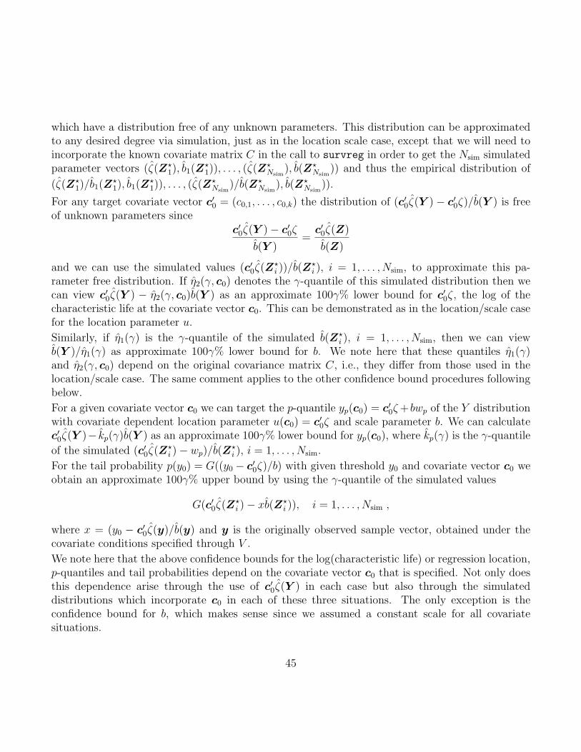
which have a distribution free of any unknown parameters. This distribution can be approximatedto any desired degree via simulation, just as in the location scale case, except that we will need toincorporate the known covariate matrix C in the call to survreg in order to get the Nsim simulatedparameter vectors (ζ(Z?
1), b1(Z?1)), . . . , (ζ(Z
?Nsim
), b(Z?Nsim
)) and thus the empirical distribution of
(ζ(Z?1)/b1(Z
?1), b1(Z
?1)), . . . , (ζ(Z
?Nsim
)/b(Z?Nsim
), b(Z?Nsim
)).
For any target covariate vector c′0 = (c0,1, . . . , c0,k) the distribution of (c′0ζ(Y )− c′0ζ)/b(Y ) is freeof unknown parameters since
c′0ζ(Y )− c′0ζ
b(Y )=
c′0ζ(Z)
b(Z)
and we can use the simulated values (c′0ζ(Z?i ))/b(Z
?i ), i = 1, . . . , Nsim, to approximate this pa-
rameter free distribution. If η2(γ, c0) denotes the γ-quantile of this simulated distribution then wecan view c′0ζ(Y ) − η2(γ, c0)b(Y ) as an approximate 100γ% lower bound for c′0ζ, the log of thecharacteristic life at the covariate vector c0. This can be demonstrated as in the location/scale casefor the location parameter u.
Similarly, if η1(γ) is the γ-quantile of the simulated b(Z?i ), i = 1, . . . , Nsim, then we can view
b(Y )/η1(γ) as approximate 100γ% lower bound for b. We note here that these quantiles η1(γ)and η2(γ, c0) depend on the original covariance matrix C, i.e., they differ from those used in thelocation/scale case. The same comment applies to the other confidence bound procedures followingbelow.
For a given covariate vector c0 we can target the p-quantile yp(c0) = c′0ζ+ bwp of the Y distributionwith covariate dependent location parameter u(c0) = c′0ζ and scale parameter b. We can calculatec′0ζ(Y )− kp(γ)b(Y ) as an approximate 100γ% lower bound for yp(c0), where kp(γ) is the γ-quantile
of the simulated (c′0ζ(Z?i )− wp)/b(Z
?i ), i = 1, . . . , Nsim.
For the tail probability p(y0) = G((y0 − c′0ζ)/b) with given threshold y0 and covariate vector c0 weobtain an approximate 100γ% upper bound by using the γ-quantile of the simulated values
G(c′0ζ(Z?i )− xb(Z?
i )), i = 1, . . . , Nsim ,
where x = (y0 − c′0ζ(y)/b(y) and y is the originally observed sample vector, obtained under thecovariate conditions specified through V .
We note here that the above confidence bounds for the log(characteristic life) or regression location,p-quantiles and tail probabilities depend on the covariate vector c0 that is specified. Not only doesthis dependence arise through the use of c′0ζ(Y ) in each case but also through the simulateddistributions which incorporate c0 in each of these three situations. The only exception is theconfidence bound for b, which makes sense since we assumed a constant scale for all covariatesituations.
45
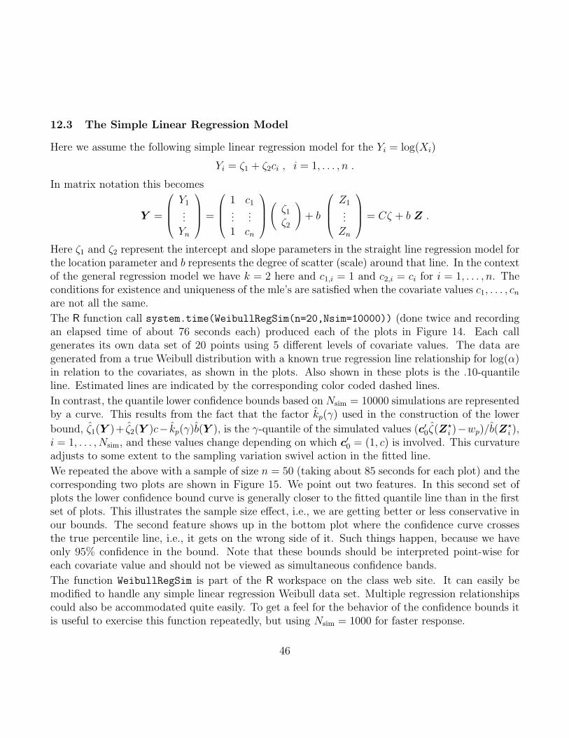
12.3 The Simple Linear Regression Model
Here we assume the following simple linear regression model for the Yi = log(Xi)
Yi = ζ1 + ζ2ci , i = 1, . . . , n .
In matrix notation this becomes
Y =
Y1...Yn
=
1 c1...
...1 cn
(ζ1ζ2
)+ b
Z1...Zn
= Cζ + b Z .
Here ζ1 and ζ2 represent the intercept and slope parameters in the straight line regression model forthe location parameter and b represents the degree of scatter (scale) around that line. In the contextof the general regression model we have k = 2 here and c1,i = 1 and c2,i = ci for i = 1, . . . , n. Theconditions for existence and uniqueness of the mle’s are satisfied when the covariate values c1, . . . , cnare not all the same.
The R function call system.time(WeibullRegSim(n=20,Nsim=10000)) (done twice and recordingan elapsed time of about 76 seconds each) produced each of the plots in Figure 14. Each callgenerates its own data set of 20 points using 5 different levels of covariate values. The data aregenerated from a true Weibull distribution with a known true regression line relationship for log(α)in relation to the covariates, as shown in the plots. Also shown in these plots is the .10-quantileline. Estimated lines are indicated by the corresponding color coded dashed lines.
In contrast, the quantile lower confidence bounds based on Nsim = 10000 simulations are representedby a curve. This results from the fact that the factor kp(γ) used in the construction of the lower
bound, ζ1(Y )+ ζ2(Y )c− kp(γ)b(Y ), is the γ-quantile of the simulated values (c′0ζ(Z?i )−wp)/b(Z
?i ),
i = 1, . . . , Nsim, and these values change depending on which c′0 = (1, c) is involved. This curvatureadjusts to some extent to the sampling variation swivel action in the fitted line.
We repeated the above with a sample of size n = 50 (taking about 85 seconds for each plot) and thecorresponding two plots are shown in Figure 15. We point out two features. In this second set ofplots the lower confidence bound curve is generally closer to the fitted quantile line than in the firstset of plots. This illustrates the sample size effect, i.e., we are getting better or less conservative inour bounds. The second feature shows up in the bottom plot where the confidence curve crossesthe true percentile line, i.e., it gets on the wrong side of it. Such things happen, because we haveonly 95% confidence in the bound. Note that these bounds should be interpreted point-wise foreach covariate value and should not be viewed as simultaneous confidence bands.
The function WeibullRegSim is part of the R workspace on the class web site. It can easily bemodified to handle any simple linear regression Weibull data set. Multiple regression relationshipscould also be accommodated quite easily. To get a feel for the behavior of the confidence bounds itis useful to exercise this function repeatedly, but using Nsim = 1000 for faster response.
46
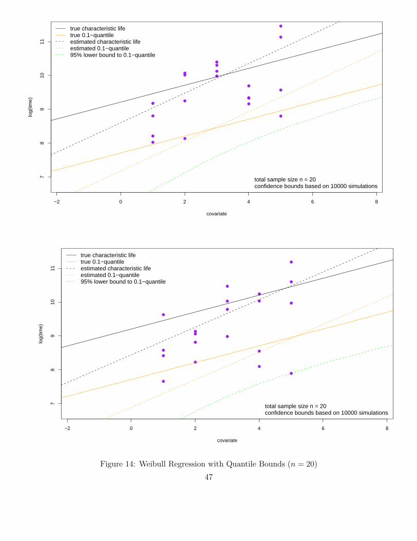
●
●
●
●
●
●●
●
●
●
●●
●
●
●●
●
●
●
●
−2 0 2 4 6 8
78
910
11
covariate
log(
time)
true characteristic lifetrue 0.1−quantileestimated characteristic lifeestimated 0.1−quantile95% lower bound to 0.1−quantile
total sample size n = 20confidence bounds based on 10000 simulations
●
●
●
●
●
●
●●
●
●
●
●
●
●
●
●
●
●
●
●
−2 0 2 4 6 8
78
910
11
covariate
log(
time)
true characteristic lifetrue 0.1−quantileestimated characteristic lifeestimated 0.1−quantile95% lower bound to 0.1−quantile
total sample size n = 20confidence bounds based on 10000 simulations
Figure 14: Weibull Regression with Quantile Bounds (n = 20)
47
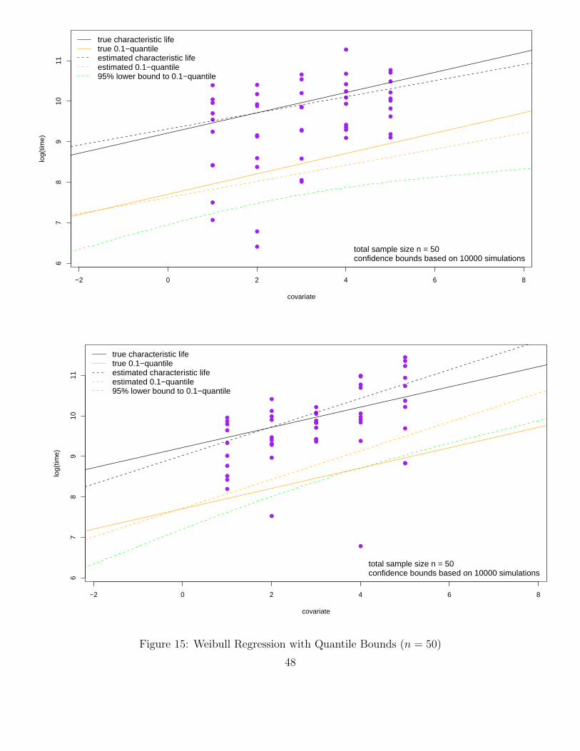
●
●
●
●
●
●
●
●
●
●
●
●
●
●
●
●
●
●
●
●
●
●
●
●
●
●
●
●●
●
●
●
●●●
●
●
●
●
●●
●
●
●●
●
●
●
●
●
−2 0 2 4 6 8
67
89
1011
covariate
log(
time)
true characteristic lifetrue 0.1−quantileestimated characteristic lifeestimated 0.1−quantile95% lower bound to 0.1−quantile
total sample size n = 50confidence bounds based on 10000 simulations
●
●
●
●
●
●
●●
●
●
●
●
●
●
●
●●
●
●
●
●
●
●
●
●
●
●
●
●
●
●
●
●●
●
●
●
●●
●
●
●
●
●
●
●●
●
●
●
−2 0 2 4 6 8
67
89
1011
covariate
log(
time)
true characteristic lifetrue 0.1−quantileestimated characteristic lifeestimated 0.1−quantile95% lower bound to 0.1−quantile
total sample size n = 50confidence bounds based on 10000 simulations
Figure 15: Weibull Regression with Quantile Bounds (n = 50)
48
12.4 The k-Sample Problem
A second illustration example concerns the situation of k = 3 samples with same scale but possiblydifferent locations. In terms of the untransformed Weibull data this means that we have possiblydifferent unknown characteristic life parameters (α1, α2, α3) but same unknown shape β for eachsample. The modifications for k 6= 3 should be obvious. In matrix notation this model is
Y =
Y1...Yn1
...Yn1+1
...Yn1+n2
Yn1+n2+1...
Yn1+n2+n3
=
1 0 0...
......
1 0 01 1 0...
......
1 1 01 0 1...
......
1 0 1
ζ1ζ2ζ3
+ b
Z1...Zn1
...Zn1+1
...Zn1+n2
Zn1+n2+1...
Zn1+n2+n3
= Cζ + b Z .
Here the Yi have location u1 = ζ1 for the first n1 observations, they have location u2 = ζ1 + ζ2 forthe next n2 observations and they have location u3 = ζ1 + ζ3 for the last n3 observations. Thus wecan consider u1 = ζ1 as the baseline location (represented by the first n1 observations), ζ2 can beconsidered as the incremental change from u1 to u2 and ζ3 is the incremental change from u1 to u3.
If we were interested in the question whether the three samples come from the same location/scalemodel we would consider testing the hypothesis H0 : ζ2 = ζ3 = 0 or equivalently H0 : u1 = u2 = u3.Instead of using the likelihood ratio test, which invokes the χ2
k−1 = χ22 distribution as approximate
null distribution, we will employ the test statistic suggested in Lawless (1982) (p. 302, equation(6.4.12)) for which the same approximate null distribution is invoked. Our reason for following thischoice is its similarity to the standard test statistic used in the corresponding normal distributionmodel, i.e., when Zi ∼ Φ(z) instead of Zi ∼ G(z) as in the above regression model. Also, themodification of this test statistic for general k(6= 3) is obvious. The formal definition of the teststatistic proposed by Lawless is as follows:
Λ1 = (ζ2, ζ3)K−111 (ζ2, ζ3)
t ,
where K11 is the asymptotic 2 × 2 covariance matrix of (ζ2, ζ3). Without going into the detailedderivation one can give the following alternate and more transparent expression for Λ1
Λ1 =
∑3i=1 ni(ui(Y )− u(Y ))2
b(Y )2,
49
where
u1(Y ) = ζ1(Y ) , u2(Y ) = ζ1(Y )+ζ2(Y ) , u3(Y ) = ζ1(Y )+ζ3(Y ) and u(Y ) =3∑
i=1
(ni/N)ui(Y ) ,
with N = n1+n1+n3. In the normal case Λ1 reduces to the traditional F -test statistic (except for aconstant multiplier, namely (n−k)/((k−1)n) = (n−3)/(2n)) when writing ui(Y ) = Yi., i = 1, 2, 3and u(Y ) = Y.. = (n1/N)Y1. + (n2/N)Y2. + (n3/N)Y3. and
b(Y )2 =1
n
k∑i=1
ni∑j=1
(Yij − Yi.)2 ,
which are the corresponding mle’s in the normal case. However, in the normal case one uses theFk−1,N−k distribution as the exact null distribution of the properly scaled Λ1 and the uncertainty
in b(Y )2 is not ignored by simply referring to the χ2k−1 distribution, using a large sample argument.
We don’t have to use a large sample approximation either, since the null distribution of Λ1 (in thelog-Weibull case) is free of any unknown parameters and can be simulated to any desired degree ofaccuracy. This is seen as follows from our equivariance properties. Recall that
u1(Y )− u1
b(Y )=ζ1(Y )− ζ1
b(Y ),ui(Y )− ui
b(Y )=ζ1(Y ) + ζi(Y )− (ζ1 + ζi)
b(Y ), i = 2, 3
have distributions free of unknown parameters. Under the hypothesis H0 when u1 = u2 = u3(= u)we thus have that
ui(Y )− u
b(Y ),
u(Y )− u
b(Y ), and thus
ui(Y )− u(Y )
b(Y )=ui(Y )− u
b(Y )− u(Y )− u
b(Y )
have distributions free of any unknown parameters which in turn implies the above claim about Λ1.
Thus we can estimate the null distribution of Λ1 by using the Nsim simulated values of ζi(Z?j)/b(Z
?j)
to create
u1(Z?j)
b(Z?j)
=ζ1(Z
?j)
b(Z?j)
,ui(Z
?j)
b(Z?j)
=ζ1(Z
?j) + ζi(Z
?j)
b(Z?j)
, i = 2, 3 andu(Z?
j)
b(Z?j)
=
∑3i=1 niui(Z
?j)/N
b(Z?j)
and thus
Λ1(Z?j) =
∑3i=1 ni(ui(Z
?j)− u(Z?
j))2
b(Z?j)
2j = 1, . . . , Nsim .
The distribution of these Nsim values Λ1(Z?j) will give a very good approximation for the true null
distribution of Λ1. The accuracy of this approximation is entirely controllable by the choice of Nsim.Nsim = 10000 should be sufficient for most practical purposes.
50
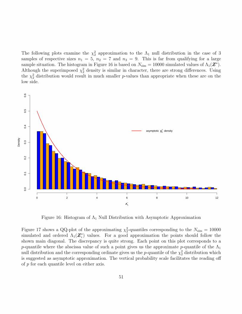
The following plots examine the χ22 approximation to the Λ1 null distribution in the case of 3
samples of respective sizes n1 = 5, n2 = 7 and n3 = 9. This is far from qualifying for a largesample situation. The histogram in Figure 16 is based on Nsim = 10000 simulated values of Λ1(Z
?).Although the superimposed χ2
2 density is similar in character, there are strong differences. Usingthe χ2
2 distribution would result in much smaller p-values than appropriate when these are on thelow side.
ΛΛ1*
Den
sity
0 2 4 6 8 10 12
0.0
0.1
0.2
0.3
0.4
0.5
0.6
asymptotic χχ22 density
Figure 16: Histogram of Λ1 Null Distribution with Asymptotic Approximation
Figure 17 shows a QQ-plot of the approximating χ22-quantiles corresponding to the Nsim = 10000
simulated and ordered Λ1(Z?i ) values. For a good approximation the points should follow the
shown main diagonal. The discrepancy is quite strong. Each point on this plot corresponds to ap-quantile where the abscissa value of such a point gives us the approximate p-quantile of the Λ1
null distribution and the corresponding ordinate gives us the p-quantile of the χ22 distribution which
is suggested as asymptotic approximation. The vertical probability scale facilitates the reading offof p for each quantile level on either axis.
51
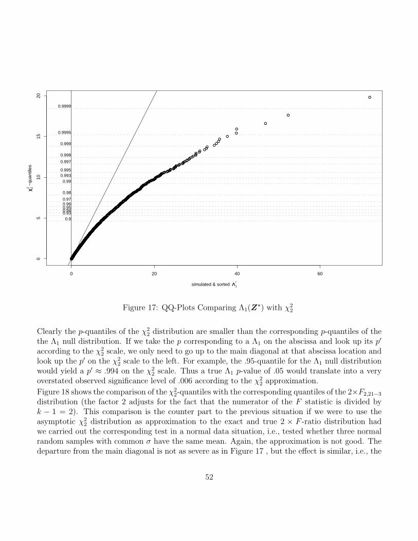
●●●●●●●●●●●●●●●●●●●●●●●●●●●●●●●●●●●●●●●●●●●●●●●●●●●●●●●●●●●●●●●●●●●●●●●●●●●●●●●●●●●●●●●●●●●●●●●●●●●●●●●●●●●●●●●●●●●●●●●●●●●●●●●●●●●●●●●●●●●●●●●●●●●●●●●●●●●●●●●●●●●●●●●●●●●●●●●●●●●●●●●●●●●●●●●●●●●●●●●●●●●●●●●●●●●●●●●●●●●●●●●●●●●●●●●●●●●●●●●●●●●●●●●●●●●●●●●●●●●●●●●●●●●●●●●●●●●●●●●●●●●●●●●●●●●●●●●●●●●●●●●●●●●●●●●●●●●●●●●●●●●●●●●●●●●●●●●●●●●●●●●●●●●●●●●●●●●●●●●●●●●●●●●●●●●●●●●●●●●●●●●●●●●●●●●●●●●●●●●●●●●●●●●●●●●●●●●●●●●●●●●●●●●●●●●●●●●●●●●●●●●●●●●●●●●●●●●●●●●●●●●●●●●●●●●●●●●●●●●●●●●●●●●●●●●●●●●●●●●●●●●●●●●●●●●●●●●●●●●●●●●●●●●●●●●●●●●●●●●●●●●●●●●●●●●●●●●●●●●●●●●●●●●●●●●●●●●●●●●●●●●●●●●●●●●●●●●●●●●●●●●●●●●●●●●●●●●●●●●●●●●●●●●●●●●●●●●●●●●●●●●●●●●●●●●●●●●●●●●●●●●●●●●●●●●●●●●●●●●●●●●●●●●●●●●●●●●●●●●●●●●●●●●●●●●●●●●●●●●●●●●●●●●●●●●●●●●●●●●●●●●●●●●●●●●●●●●●●●●●●●●●●●●●●●●●●●●●●●●●●●●●●●●●●●●●●●●●●●●●●●●●●●●●●●●●●●●●●●●●●●●●●●●●●●●●●●●●●●●●●●●●●●●●●●●●●●●●●●●●●●●●●●●●●●●●●●●●●●●●●●●●●●●●●●●●●●●●●●●●●●●●●●●●●●●●●●●●●●●●●●●●●●●●●●●●●●●●●●●●●●●●●●●●●●●●●●●●●●●●●●●●●●●●●●●●●●●●●●●●●●●●●●●●●●●●●●●●●●●●●●●●●●●●●●●●●●●●●●●●●●●●●●●●●●●●●●●●●●●●●●●●●●●●●●●●●●●●●●●●●●●●●●●●●●●●●●●●●●●●●●●●●●●●●●●●●●●●●●●●●●●●●●●●●●●●●●●●●●●●●●●●●●●●●●●●●●●●●●●●●●●●●●●●●●●●●●●●●●●●●●●●●●●●●●●●●●●●●●●●●●●●●●●●●●●●●●●●●●●●●●●●●●●●●●●●●●●●●●●●●●●●●●●●●●●●●●●●●●●●●●●●●●●●●●●●●●●●●●●●●●●●●●●●●●●●●●●●●●●●●●●●●●●●●●●●●●●●●●●●●●●●●●●●●●●●●●●●●●●●●●●●●●●●●●●●●●●●●●●●●●●●●●●●●●●●●●●●●●●●●●●●●●●●●●●●●●●●●●●●●●●●●●●●●●●●●●●●●●●●●●●●●●●●●●●●●●●●●●●●●●●●●●●●●●●●●●●●●●●●●●●●●●●●●●●●●●●●●●●●●●●●●●●●●●●●●●●●●●●●●●●●●●●●●●●●●●●●●●●●●●●●●●●●●●●●●●●●●●●●●●●●●●●●●●●●●●●●●●●●●●●●●●●●●●●●●●●●●●●●●●●●●●●●●●●●●●●●●●●●●●●●●●●●●●●●●●●●●●●●●●●●●●●●●●●●●●●●●●●●●●●●●●●●●●●●●●●●●●●●●●●●●●●●●●●●●●●●●●●●●●●●●●●●●●●●●●●●●●●●●●●●●●●●●●●●●●●●●●●●●●●●●●●●●●●●●●●●●●●●●●●●●●●●●●●●●●●●●●●●●●●●●●●●●●●●●●●●●●●●●●●●●●●●●●●●●●●●●●●●●●●●●●●●●●●●●●●●●●●●●●●●●●●●●●●●●●●●●●●●●●●●●●●●●●●●●●●●●●●●●●●●●●●●●●●●●●●●●●●●●●●●●●●●●●●●●●●●●●●●●●●●●●●●●●●●●●●●●●●●●●●●●●●●●●●●●●●●●●●●●●●●●●●●●●●●●●●●●●●●●●●●●●●●●●●●●●●●●●●●●●●●●●●●●●●●●●●●●●●●●●●●●●●●●●●●●●●●●●●●●●●●●●●●●●●●●●●●●●●●●●●●●●●●●●●●●●●●●●●●●●●●●●●●●●●●●●●●●●●●●●●●●●●●●●●●●●●●●●●●●●●●●●●●●●●●●●●●●●●●●●●●●●●●●●●●●●●●●●●●●●●●●●●●●●●●●●●●●●●●●●●●●●●●●●●●●●●●●●●●●●●●●●●●●●●●●●●●●●●●●●●●●●●●●●●●●●●●●●●●●●●●●●●●●●●●●●●●●●●●●●●●●●●●●●●●●●●●●●●●●●●●●●●●●●●●●●●●●●●●●●●●●●●●●●●●●●●●●●●●●●●●●●●●●●●●●●●●●●●●●●●●●●●●●●●●●●●●●●●●●●●●●●●●●●●●●●●●●●●●●●●●●●●●●●●●●●●●●●●●●●●●●●●●●●●●●●●●●●●●●●●●●●●●●●●●●●●●●●●●●●●●●●●●●●●●●●●●●●●●●●●●●●●●●●●●●●●●●●●●●●●●●●●●●●●●●●●●●●●●●●●●●●●●●●●●●●●●●●●●●●●●●●●●●●●●●●●●●●●●●●●●●●●●●●●●●●●●●●●●●●●●●●●●●●●●●●●●●●●●●●●●●●●●●●●●●●●●●●●●●●●●●●●●●●●●●●●●●●●●●●●●●●●●●●●●●●●●●●●●●●●●●●●●●●●●●●●●●●●●●●●●●●●●●●●●●●●●●●●●●●●●●●●●●●●●●●●●●●●●●●●●●●●●●●●●●●●●●●●●●●●●●●●●●●●●●●●●●●●●●●●●●●●●●●●●●●●●●●●●●●●●●●●●●●●●●●●●●●●●●●●●●●●●●●●●●●●●●●●●●●●●●●●●●●●●●●●●●●●●●●●●●●●●●●●●●●●●●●●●●●●●●●●●●●●●●●●●●●●●●●●●●●●●●●●●●●●●●●●●●●●●●●●●●●●●●●●●●●●●●●●●●●●●●●●●●●●●●●●●●●●●●●●●●●●●●●●●●●●●●●●●●●●●●●●●●●●●●●●●●●●●●●●●●●●●●●●●●●●●●●●●●●●●●●●●●●●●●●●●●●●●●●●●●●●●●●●●●●●●●●●●●●●●●●●●●●●●●●●●●●●●●●●●●●●●●●●●●●●●●●●●●●●●●●●●●●●●●●●●●●●●●●●●●●●●●●●●●●●●●●●●●●●●●●●●●●●●●●●●●●●●●●●●●●●●●●●●●●●●●●●●●●●●●●●●●●●●●●●●●●●●●●●●●●●●●●●●●●●●●●●●●●●●●●●●●●●●●●●●●●●●●●●●●●●●●●●●●●●●●●●●●●●●●●●●●●●●●●●●●●●●●●●●●●●●●●●●●●●●●●●●●●●●●●●●●●●●●●●●●●●●●●●●●●●●●●●●●●●●●●●●●●●●●●●●●●●●●●●●●●●●●●●●●●●●●●●●●●●●●●●●●●●●●●●●●●●●●●●●●●●●●●●●●●●●●●●●●●●●●●●●●●●●●●●●●●●●●●●●●●●●●●●●●●●●●●●●●●●●●●●●●●●●●●●●●●●●●●●●●●●●●●●●●●●●●●●●●●●●●●●●●●●●●●●●●●●●●●●●●●●●●●●●●●●●●●●●●●●●●●●●●●●●●●●●●●●●●●●●●●●●●●●●●●●●●●●●●●●●●●●●●●●●●●●●●●●●●●●●●●●●●●●●●●●●●●●●●●●●●●●●●●●●●●●●●●●●●●●●●●●●●●●●●●●●●●●●●●●●●●●●●●●●●●●●●●●●●●●●●●●●●●●●●●●●●●●●●●●●●●●●●●●●●●●●●●●●●●●●●●●●●●●●●●●●●●●●●●●●●●●●●●●●●●●●●●●●●●●●●●●●●●●●●●●●●●●●●●●●●●●●●●●●●●●●●●●●●●●●●●●●●●●●●●●●●●●●●●●●●●●●●●●●●●●●●●●●●●●●●●●●●●●●●●●●●●●●●●●●●●●●●●●●●●●●●●●●●●●●●●●●●●●●●●●●●●●●●●●●●●●●●●●●●●●●●●●●●●●●●●●●●●●●●●●●●●●●●●●●●●●●●●●●●●●●●●●●●●●●●●●●●●●●●●●●●●●●●●●●●●●●●●●●●●●●●●●●●●●●●●●●●●●●●●●●●●●●●●●●●●●●●●●●●●●●●●●●●●●●●●●●●●●●●●●●●●●●●●●●●●●●●●●●●●●●●●●●●●●●●●●●●●●●●●●●●●●●●●●●●●●●●●●●●●●●●●●●●●●●●●●●●●●●●●●●●●●●●●●●●●●●●●●●●●●●●●●●●●●●●●●●●●●●●●●●●●●●●●●●●●●●●●●●●●●●●●●●●●●●●●●●●●●●●●●●●●●●●●●●●●●●●●●●●●●●●●●●●●●●●●●●●●●●●●●●●●●●●●●●●●●●●●●●●●●●●●●●●●●●●●●●●●●●●●●●●●●●●●●●●●●●●●●●●●●●●●●●●●●●●●●●●●●●●●●●●●●●●●●●●●●●●●●●●●●●●●●●●●●●●●●●●●●●●●●●●●●●●●●●●●●●●●●●●●●●●●●●●●●●●●●●●●●●●●●●●●●●●●●●●●●●●●●●●●●●●●●●●●●●●●●●●●●●●●●●●●●●●●●●●●●●●●●●●●●●●●●●●●●●●●●●●●●●●●●●●●●●●●●●●●●●●●●●●●●●●●●●●●●●●●●●●●●●●●●●●●●●●●●●●●●●●●●●●●●●●●●●●●●●●●●●●●●●●●●●●●●●●●●●●●●●●●●●●●●●●●●●●●●●●●●●●●●●●●●●●●●●●●●●●●●●●●●●●●●●●●●●●●●●●●●●●●●●●●●●●●●●●●●●●●●●●●●●●●●●●●●●●●●●●●●●●●●●●●●●●●●●●●●●●●●●●●●●●●●●●●●●●●●●●●●●●●●●●●●●●●●●●●●●●●●●●●●●●●●●●●●●●●●●●●●●●●●●●●●●●●●●●●●●●●●●●●●●●●●●●●●●●●●●●●●●●●●●●●●●●●●●●●●●●●●●●●●●●●●●●●●●●●●●●●●●●●●●●●●●●●●●●●●●●●●●●●●●●●●●●●●●●●●●●●●●●●●●●●●●●●●●●●●●●●●●●●●●●●●●●●●●●●●●●●●●●●●●●●●●●●●●●●●●●●●●●●●●●●●●●●●●●●●●●●●●●●●●●●●●●●●●●●●●●●●●●●●●●●●●●●●●●●●●●●●●●●●●●●●●●●●●●●●●●●●●●●●●●●●●●●●●●●●●●●●●●●●●●●●●●●●●●●●●●●●●●●●●●●●●●●●●●●●●●●●●●●●●●●●●●●●●●●●●●●●●●●●●●●●●●●●●●●●●●●●●●●●●●●●●●●●●●●●●●●●●●●●●●●●●●●●●●●●●●●●●●●●●●●●●●●●●●●●●●●●●●●●●●●●●●●●●●●●●●●●●●●●●●●●●●●●●●●●●●●●●●●●●●●●●●●●●●●●●●●●●●●●●●●●●●●●●●●●●●●●●●●●●●●●●●●●●●●●●●●●●●●●●●●●●●●●●●●●●●●●●●●●●●●●●●●●●●●●●●●●●●●●●●●●●●●●●●●●●●●●●●●●●●●●●●●●●●●●●●●●●●●●●●●●●●●●●●●●●●●●●●●●●●●●●●●●●●●●●●●●●●●●●●●●●●●●●●●●●●●●●●●●●●●●●●●●●●●●●●●●●●●●●●●●●●●●●●●●●●●●●●●●●●●●●●●●●●●●●●●●●●●●●●●●●●●●●●●●●●●●●●●●●●●●●●●●●●●●●●●●●●●●●●●●●●●●●●●●●●●●●●●●●●●●●●●●●●●●●●●●●●●●●●●●●●●●●●●●●●●●●●●●●●●●●●●●●●●●●●●●●●●●●●●●●●●●●●●●●●●●●●●●●●●●●●●●●●●●●●●●●●●●●●●●●●●●●●●●●●●●●●●●●●●●●●●●●●●●●●●●●●●●●●●●●●●●●●●●●●●●●●●●●●●●●●●●●●●●●●●●●●●●●●●●●●●●●●●●●●●●●●●●●●●●●●●●●●●●●●●●●●●●●●●●●●●●●●●●●●●●●●●●●●●●●●●●●●●●●●●●●●●●●●●●●●●●●●●●●●●●●●●●●●●●●●●●●●●●●●●●●●●●●●●●●●●●●●●●●●●●●●●●●●●●●●●●●●●●●●●●●●●●●●●●●●●●●●●●●●●●●●●●●●●●●●●●●●●●●●●●●●●●●●●●●●●●●●●●●●●●●●●●●●●●●●●●●●●●●●●●●●●●●●●●●●●●●●●●●●●●●●●●●●●●●●●●●●●●●●●●●●●●●●●●●●●●●●●●●●●●●●●●●●●●●●●●●●●●●●●●●●●●●●●●●●●●●●●●●●●●●●●●●●●●●●●●●●●●●●●●●●●●●●●●●●●●●●●●●●●●●●●●●●●●●●●●●●●●●●●●●●●●●●●●●●●●●●●●●●●●●●●●●●●●●●●●●●●●●●●●●●●●●●●●●●●●●●●●●●●●●●●●●●●●●●●●●●●●●●●●●●●●●●●●●●●●●●●●●●●●●●●●●●●●●●●●●●●●●●●●●●●●●●●●●●●●●●●●●●●●●●●●●●●●●●●●●●●●●●●●●●●●●●●●●●●●●●●●●●●●●●●●●●●●●●●●●●●●●●●●●●●●●●●●●●●●●●●●●●●●●●●●●●●●●●●●●●●●●●●●●●●●●●●●●●●●●●●●●●●●●●●●●●●●●●●●●●●●●●●●●●●●●●●●●●●●●●●●●●●●●●●●●●●●●●●●●●●●●●●●●●●●●●●●●●●●●●●●●●●●●●●●●●●●●●●●●●●●●●●●●●●●●●●●●●●●●●●●●●●●●●●●●●●●●●●●●●●●●●●●●●●●●●●●●●●●●●●●●●●●●●●●●●●●●●●●●●●●●●●●●●●●●●●●●●●●●●●●●●●●●●●●●●●●●●●●●●●●●●●●●●●●●●●●●●●●●●●●●●●●●●●●●●●●●●●●●●●●●●●●●●●●●●●●●●●●●●●●●●●●●●●●●●●●●●●●●●●●●●●●●●●●●●●●●●●●●●●●●●●●●●●●●●●●●●●●●●●●●●●●●●●●●●●●●●●●●●●●●●●●●●●●●●●●●●●●●●●●●●●●●●●●●●●●●●●●●●●●●●●●●●●●●●●●●●●●●●●●●●●●●●●●●●●●●●●●●●●●●●●●●●●●●●●●●●●●●●●●●●●●●●●●●●●●●●●●●●●●●●●●●●●●●●●●●●●●●●●●●●●●●●●●●●●●●●●●●●●●●●●●●●●●●●●●●●●●●●●●●●●●●●●●●●●●●●●●●●●●●●●●●●●●●●●●●●●●●●●●●●●●●●●●●●●●●●●●●●●●●●●●●●●●●●●●●●●●●●●●●●●●●●●●●●●●●●●●●●●●●●●●●●●●●●●●●●●●●●●●●●●●●●●●●●●●●●●●●●●●●●●●●●●●●●●●●●●●●●●●●●●●●●●●●●●●●●●●●●●●●●●●●●●●●●●●●●●●●●●●●●●●●●●●●●●●●●●●●●●●●●●●●●●●●●●●●●●●●●●●●●●●●●●●●●●●●●●●●●●●●●●●●●●●●●●●●●●●●●●●●●●●●●●●●●●●●●●●●●●●●●●●●●●●●●●●●●●●●●●●●●●●●●●●●●●●●●●●●●●●●●●●●●●●●●●●●●●●●●●●●●●●●●●●●●●●●●●●●●●●●●●●●●●●●●●●●●●●●●●●●●●●●●●●●●●●●●●●●●●●●●●●●●●●●●●●●●●●●●●●●●●●●●●●●●●●●●●●●●●●●●●●●●●●●●●●●●●●●●●●●●●●●●●●●●●●●●●●●●●●●●●●●●●●●●●●●●●●●●●●●●●●●●●●●●●●●●●●●●●●●●●●●●●●●●●●●●●●●●●●●●●●●●●●●●●●●●●●●●●●●●●●●●●●●●●●●●●●●●●●●●●●●●●●●●●●●●●●●●●●●●●●●●●●●●●●●●●●●●●●●●●●●●●●●●●●●●●●●●●●●●●●●●●●●●●●●●●●●●●●●●●●●●●●●●●●●●●●●●●●●●●●●●●●●●●●●●●●●●●●●●●●●●●●●●●●●●●●●●●●●●●●●●●●●●●●●●●●●●●●●●●●●●●●●●●●●●●●●●●●●●●●●●●●●●●●●●●●●●●●●●●●●●●●●●●●●●●●●●●●●●●●●●●●●●●●●●●●●●●●●●●●●●●●●●●●●●●●●●●●●●●●●●●●●●●●●●●●●●●●●●●●●●●●●●●●●●●●●●●●●●●●●●●●●●●●●●●●●●●●●●●●●●●●●●●●●●●●●●●●●●●●●●●●●●●●●●●●●●●●●●●●●●●●●●●●●●●●●●●●●●●●●●●●●●●●●●●●●●●●●●●●●●●●●●●●●●●●●●●●●●●●●●●●●●●●●●●●●●●●●●●●●●●●●●●●●●●●●●●●●●●●●●●●●●●●●●●●●●●●●●●●●●●●●●●●●●●●●●●●●●●●●●●●●●●●●●●●●●●●●●●●●●●●●●●●●●●●●●●●●●●●●●●●●●●●●●●●●●●●●●●●●●●●●●●●●●●●●●●●●●●●●●●●●●●●●●●●●●●●●●●●●●●●●●●●●●●●●●●●●●●●●●●●●●●●●●●●●●●●●●●●●●●●●●●●●●●●●●●●●●●●●●●●●●●●●●●●●●●●●●●●●●●●●●●●●●●●●●●●●●●●●●●●●●●●●●●●●●●●●●●●●●●●●●●●●●●●●●●●●●●●●●●●●●●●●●●●●●●●●●●●●●●●●●●●●●●●●●●●●●●●●●●●●●●●●●●●●●●●●●●●●●●●●●●●●●●●●●●●●●●●●●●●●●●●●●●●●●●●●●●●●●●●●●●●●●●●●●●●●●●●●●●●●●●●●●●●●●●●●●●●●●●●●●●●●●●●●●●●●●●●●●●●●●●●●●●●●●●●●●●●●●●●●●●●●●●●●●●●●●●●●●●●●●●●●●●●●●●●●●●●●●●●●●●●●●●●●●●●●●●●●●●●●●●●●●●●●●●●●●●●●●●●●●●●●●●●●●●●●●●●●●●●●●●●●●●●●●●●●●●●●●●●●●●●●●●●●●●●●●●●●●●●●●●●●●●●●●●●●●●●●●●●●●●●●●●●●●●●●●●●●●●●●●●●●●●●●●●●●●●●●●●●●●●●●●●●●●●●●●●●●●●●●●●●●●●●●●●●●●●●●●●●●●●●●●●●●●●●●●●●●●●●●●●●●●●●●●●●●●●●●●●●●●●●●●●●●●●●●●●●●●●●●●●●●●●●●●●●●●●●●●●●●●●●●●●●●●●●●●●●●●●●●●●●●●●●●●●●●●●●●●●●●●●●●●●●●●●●●●●●●●●●●●●●●●●●●●●●●●●●●●●●●●●●●●●●●●●●●●●●●●●●●●●●●●●●●●●●●●●●●●●●●●●●●●●●●●●●●●●●●●●●●●●●●●●●●●●●●●●●●●●●●●●●●●●●●●●●●●●●●●●●●●●●●●●●●●●●●●●●●●●●●●●●●●●●●●●●●●●●●●●●●●●●●●●●●●●●●●●●●●●●●●●●●●●●●●●●●●●●●●●●●●●●●●●●●●●●●●●●●●●●●●●●●●●●●●●●●●●●●●●●●●●●●●●●●●●●●●●●●●●●●●●●●●●●●●●●●●●●●●●●●●●●●●●●●●●●●●●●●●●●●●●●●●●●●●●●●●●●●●●●●●●●●●●●●●●●●●●●●●●●●●●●●●●●●●●●●●●●●●●●●●●●●●●●●●●●●●●●●●●●●●●●●●●●●●●●●●●●●●●●●●●●●●●●●●●●●●●●●●●●●●●●●●●●●●●●●●●●●●●●●●●●●●●●●●●●●●●●●●●●●●●●●●●●●●●●●●●●●●●●●●●●●●●●●●●●●●●●●●●●●●●●●●●●●●●●●●●●●●●●●●●●●●●●●●●●●●●●●●●●●●●●●●●●●●●●●●●●●●●●●●●●●●●●●●●●●●●●●●●●●●●●●●●●●●●●●●●●●●●●●●●●●●●●●●●●●●●●●●●●●●●●●●●●●●●●●●●●●●●●●●●●●●●●●●●●●●●●●●●●●●●●●●●●●●●●●●●●●●●●●●●●●●●●●●●●●
●●●●●●●●●●●●●●●●●●●●●●●●●●●●●●●●●●●●●●●●●●●●●●●●●●●●●●●●●●●●●●●●●●●●●●●●●●●●●●●●●●●●●●●●
●●●●●●●●●●●●●●●●●●●●●●●●●●●●●●●●●●●●●●●●●●●●●●●●●●●●●●●●●●●●●●●●●●●●●●●●●●●
●●●●●●●●●●●●●●●●●●●●●●●●●●●●●●●●●●●●●●●●●●●●●●●●●●●●●●●●●●●●●●●●●●●●●●●●●●●●●●●●●●●●●●●●●●●
●●●●●●●●●●●●●●●●●●●●●●●●●●●●●●●●●●●●●●●●●●●●●●●●●●●●●●●●●●●●●●●●●●●●●●●●●●●●●●●●●●●●●●●●●
●●●●●●●●●●●●●●●●●●●●●●●●●●●●●●●●●●●
●●●●●●●●●●●●●●●●●●●●●●●●●●●●●
●●●●●●●●●●●●●●●●●●●●●●●●●●●●●●●●●●●●●●●●●●●●●●
●●●●●●●●●●●●●●●●●
●●●●●●●●●●●●●●●
●●●●●●●●●●●●●
●●●●●●●●●●
●●●●●●●●●●● ●●●●
●●●●●●●
●●●●●●●
●●●●●
●●● ●●
●●●
●●
●●
●●
●
●
●
●
0 20 40 60
05
1015
20
simulated & sorted ΛΛ1*
0.9999
0.9995
0.999
0.998
0.997
0.9950.9930.99
0.98
0.970.960.950.940.93
0.9
χχ 22 −qu
antil
es
Figure 17: QQ-Plots Comparing Λ1(Z?) with χ2
2
Clearly the p-quantiles of the χ22 distribution are smaller than the corresponding p-quantiles of the
the Λ1 null distribution. If we take the p corresponding to a Λ1 on the abscissa and look up its p′
according to the χ22 scale, we only need to go up to the main diagonal at that abscissa location and
look up the p′ on the χ22 scale to the left. For example, the .95-quantile for the Λ1 null distribution
would yield a p′ ≈ .994 on the χ22 scale. Thus a true Λ1 p-value of .05 would translate into a very
overstated observed significance level of .006 according to the χ22 approximation.
Figure 18 shows the comparison of the χ22-quantiles with the corresponding quantiles of the 2×F2,21−3
distribution (the factor 2 adjusts for the fact that the numerator of the F statistic is divided byk − 1 = 2). This comparison is the counter part to the previous situation if we were to use theasymptotic χ2
2 distribution as approximation to the exact and true 2 × F -ratio distribution hadwe carried out the corresponding test in a normal data situation, i.e., tested whether three normalrandom samples with common σ have the same mean. Again, the approximation is not good. Thedeparture from the main diagonal is not as severe as in Figure 17 , but the effect is similar, i.e., the
52
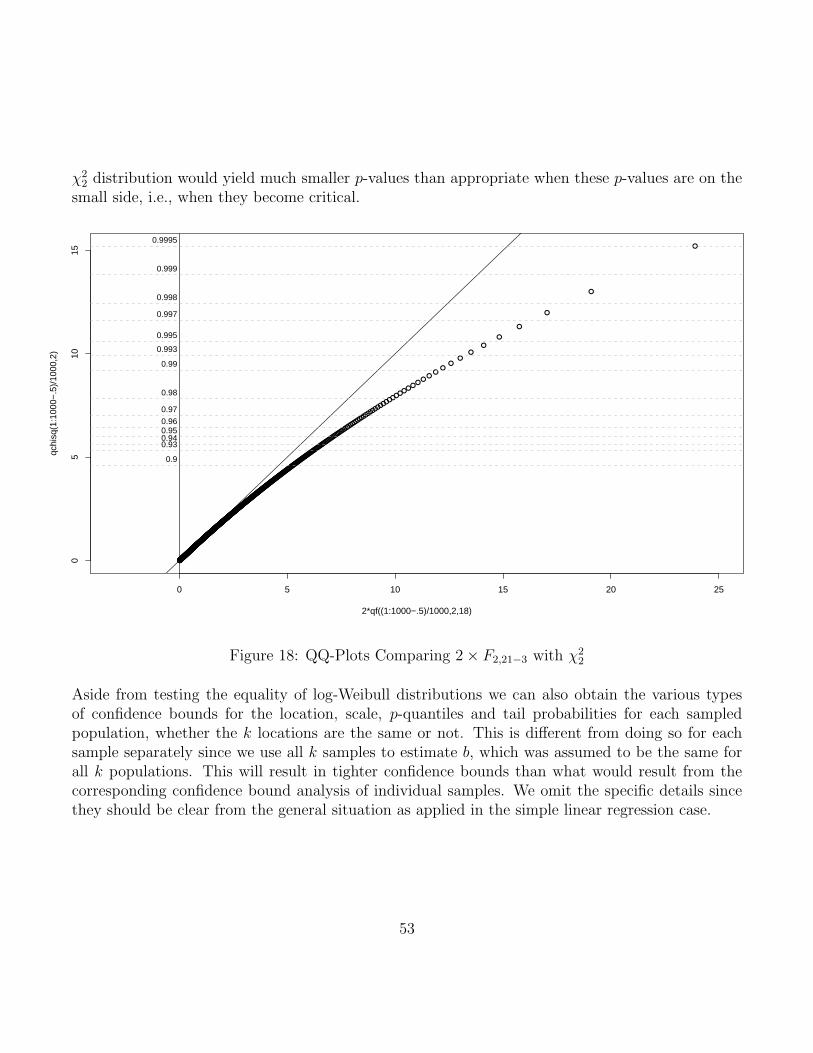
χ22 distribution would yield much smaller p-values than appropriate when these p-values are on the
small side, i.e., when they become critical.
●●●●●●●●●●●●●●●●●●●●●●●●●●●●●●●●●●●●●●●●●●●●●●●●●●●●●●●●●●●●●●●●●●●●●●●●●●●●●●●●●●●●●●●●●●●●●●●●●●●●●●●●●●●●●●●●●●●●●●●●●●●●●●●●●●●●●●●●●●●●●●●●●●●●●●●●●●●●●●●●●●●●●●●●●●●●●●●●●●●●●●●●●●●●●●●●●●●●●●●●●●●●●●●●●●●●●●●●●●●●●●●●●●●●●●●●●●●●●●●●●●●●●●●●●●●●●●●●●●●●●●●●●●●●●●●●●●●●●●●●●●●●●●●●●●●●●●●●●●●●●●●●●●●●●●●●●●●●●●●●●●●●●●●●●●●●●●●●●●●●●●●●●●●●●●●●●●●●●●●●●●●●●●●●●●●●●●●●●●●●●●●●●●●●●●●●●●●●●●●●●●●●●●●●●●●●●●●●●●●●●●●●●●●●●●●●●●●●●●●●●●●●●●●●●●●●●●●●●●●●●●●●●●●●●●●●●●●●●●●●●●●●●●●●●●●●●●●●●●●●●●●●●●●●●●●●●●●●●●●●●●●●●●●●●●●●●●●●●●●●●●●●●
●●●●●●●●●●●●●●●●●●●●●●●●●●●●●●●●●●●●●●●●●●●●●●●●●●●●●●●●
●●●●●●●●●●●●●●●●●●●●●●●●●●●●●●●●●●●●●●●●●●●●●●●●●●
●●●●●●●●●●●●●●●●●●●●●●●●●●●●●●●●●●●●●●●●●●●
●●●●●●●●●●●●●●●●●●●●●●●●●●●●●●●●●●●●●●
●●●●●●●●●●●●●●●●●●●●●●●●●●●●●●●●●
●●●●●●●●●●●●●●●●●●●●●●●●●●●●●
●●●●●●●●●●●●●●●●●●●●●●●●●●
●●●●●●●●●●●●●●●●●●●●●●●
●●●●●●●●●●●●●●●●●●●●
●●●●●●●●●●●●●●●●●●
●●●●●●●●●●●●●●●
●●●●●●●●●●●●●●
●●●●●●●●●●●●
●●●●●●●●●●
●●●●●●●●●
●●●●●●●●
●●●●●●●
●●●●●●
●●●●●●
●●●●
●●●●●●●●●●●●●●
●●
●●
●●
●●
●
●
●
●
●
●
0 5 10 15 20 25
05
1015
2*qf((1:1000−.5)/1000,2,18)
qchi
sq(1
:100
0−.5
)/10
00,2
)
0.9995
0.999
0.998
0.997
0.995
0.993
0.99
0.98
0.97
0.960.950.940.93
0.9
Figure 18: QQ-Plots Comparing 2× F2,21−3 with χ22
Aside from testing the equality of log-Weibull distributions we can also obtain the various typesof confidence bounds for the location, scale, p-quantiles and tail probabilities for each sampledpopulation, whether the k locations are the same or not. This is different from doing so for eachsample separately since we use all k samples to estimate b, which was assumed to be the same forall k populations. This will result in tighter confidence bounds than what would result from thecorresponding confidence bound analysis of individual samples. We omit the specific details sincethey should be clear from the general situation as applied in the simple linear regression case.
53
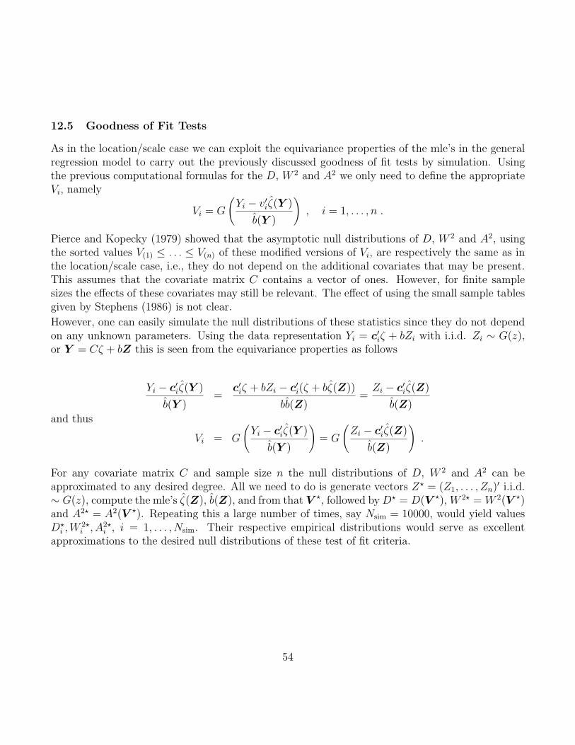
12.5 Goodness of Fit Tests
As in the location/scale case we can exploit the equivariance properties of the mle’s in the generalregression model to carry out the previously discussed goodness of fit tests by simulation. Usingthe previous computational formulas for the D, W 2 and A2 we only need to define the appropriateVi, namely
Vi = G
(Yi − v′iζ(Y )
b(Y )
), i = 1, . . . , n .
Pierce and Kopecky (1979) showed that the asymptotic null distributions of D, W 2 and A2, usingthe sorted values V(1) ≤ . . . ≤ V(n) of these modified versions of Vi, are respectively the same as inthe location/scale case, i.e., they do not depend on the additional covariates that may be present.This assumes that the covariate matrix C contains a vector of ones. However, for finite samplesizes the effects of these covariates may still be relevant. The effect of using the small sample tablesgiven by Stephens (1986) is not clear.
However, one can easily simulate the null distributions of these statistics since they do not dependon any unknown parameters. Using the data representation Yi = c′iζ + bZi with i.i.d. Zi ∼ G(z),or Y = Cζ + bZ this is seen from the equivariance properties as follows
Yi − c′iζ(Y )
b(Y )=
c′iζ + bZi − c′i(ζ + bζ(Z))
bb(Z)=Zi − c′iζ(Z)
b(Z)
and thus
Vi = G
(Yi − c′iζ(Y )
b(Y )
)= G
(Zi − c′iζ(Z)
b(Z)
).
For any covariate matrix C and sample size n the null distributions of D, W 2 and A2 can beapproximated to any desired degree. All we need to do is generate vectors Z? = (Z1, . . . , Zn)′ i.i.d.∼ G(z), compute the mle’s ζ(Z), b(Z), and from that V ?, followed byD? = D(V ?), W 2? = W 2(V ?)and A2? = A2(V ?). Repeating this a large number of times, say Nsim = 10000, would yield valuesD?
i ,W2?i , A2?
i , i = 1, . . . , Nsim. Their respective empirical distributions would serve as excellentapproximations to the desired null distributions of these test of fit criteria.
54
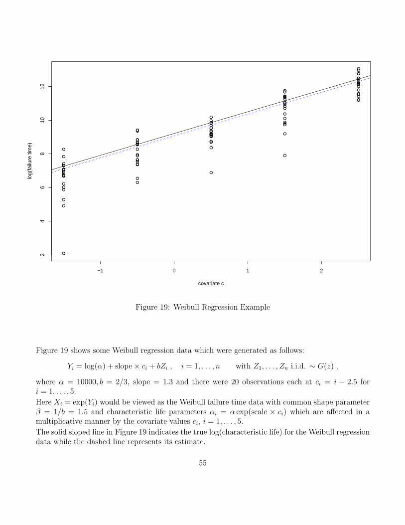
●
●
●
●
●
●
●●
●
●
●
●
●
●●
●
●
●
●
●
●
●
●
●
●
●●
●
●
●
●
●
●●
●
●
●
●
●
●
●●
●
●
●
●
●
●●
●
●
●
●
●
●●●
●
●
●
●
●
●
●
●
●●
●
●
●
●
●●
●
●
●
●
●
●●
●
●
●●
●
●
●
●
●
●
●
●●
●●
●●
●
●
●
−1 0 1 2
24
68
1012
covariate c
log(
failu
re ti
me)
Figure 19: Weibull Regression Example
Figure 19 shows some Weibull regression data which were generated as follows:
Yi = log(α) + slope× ci + bZi , i = 1, . . . , n with Z1, . . . , Zn i.i.d. ∼ G(z) ,
where α = 10000, b = 2/3, slope = 1.3 and there were 20 observations each at ci = i − 2.5 fori = 1, . . . , 5.
Here Xi = exp(Yi) would be viewed as the Weibull failure time data with common shape parameterβ = 1/b = 1.5 and characteristic life parameters αi = α exp(scale × ci) which are affected in amultiplicative manner by the covariate values ci, i = 1, . . . , 5.
The solid sloped line in Figure 19 indicates the true log(characteristic life) for the Weibull regressiondata while the dashed line represents its estimate.
55
n == 100 , Nsim == 10000
D*
Fre
quen
cy
0.00 0.02 0.04 0.06 0.08 0.10 0.12
040
080
012
00 p−value = 0.7746
D == 0.0501
W2*
Fre
quen
cy
0.00 0.05 0.10 0.15 0.20 0.25 0.30 0.35
050
010
0020
00 p−value = 0.8001
W2 == 0.0325
A2*
Fre
quen
cy
0.0 0.5 1.0 1.5
050
010
0015
00
p−value = 0.7135
A2 == 0.263
Figure 20: Weibull Goodness of Fit for Weibull Regression Example
For this generated Weibull regression data set Figure 20 shows the results of the Weibull goodnessof fit tests in relation to the simulated null distributions for the test criteria D, W 2 and A2. Thehypothesis of a Weibull lifetime distribution cannot be rejected by any of the three test of fit criteriabased on the shown p-values.
This example was produced by the R function WeibullRegGOF available in the R workspace on theclass web site. It took 105 seconds on my laptop. This function performs Weibull goodness of fittests for any supplied regression data set. When this data set is missing it generates its own Weibullregression data set of size n = 100 and uses the indicated covariates and parameters.
56
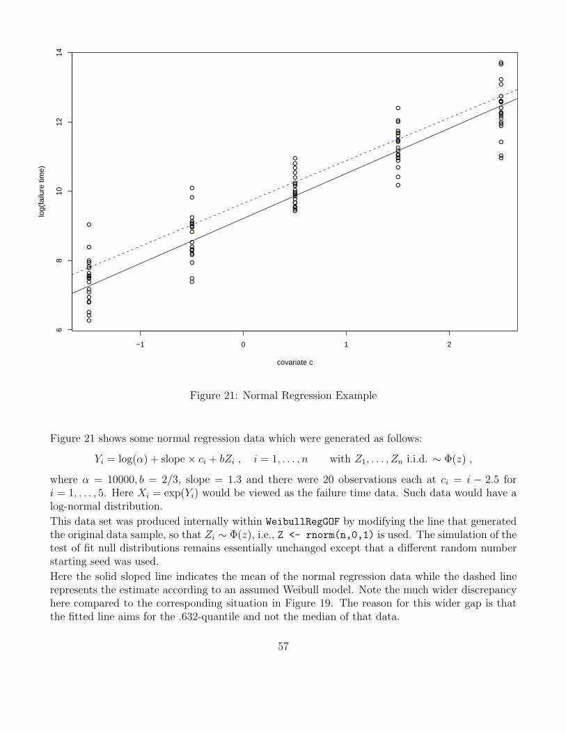
●
●
●
●
●
●
●
●
●
●
●
●
●
●
●
●
●
●
●
●
●
●
●
●●
●
●●
●
●
●
●
●
●
●
●
●
●
●●
●●
●
●
●
●
●
●
●
●
●
●
●
●
●
●●●
●
●
●
●
●
●
●
●
●●
●●
●
●
●
●
●
●
●
●
●
●
●●
●
●
●
●
●
●
●●
●
●●
●
●
●
●●
●
●
−1 0 1 2
68
1012
14
covariate c
log(
failu
re ti
me)
Figure 21: Normal Regression Example
Figure 21 shows some normal regression data which were generated as follows:
Yi = log(α) + slope× ci + bZi , i = 1, . . . , n with Z1, . . . , Zn i.i.d. ∼ Φ(z) ,
where α = 10000, b = 2/3, slope = 1.3 and there were 20 observations each at ci = i − 2.5 fori = 1, . . . , 5. Here Xi = exp(Yi) would be viewed as the failure time data. Such data would have alog-normal distribution.
This data set was produced internally within WeibullRegGOF by modifying the line that generatedthe original data sample, so that Zi ∼ Φ(z), i.e., Z <- rnorm(n,0,1) is used. The simulation of thetest of fit null distributions remains essentially unchanged except that a different random numberstarting seed was used.
Here the solid sloped line indicates the mean of the normal regression data while the dashed linerepresents the estimate according to an assumed Weibull model. Note the much wider discrepancyhere compared to the corresponding situation in Figure 19. The reason for this wider gap is thatthe fitted line aims for the .632-quantile and not the median of that data.
57
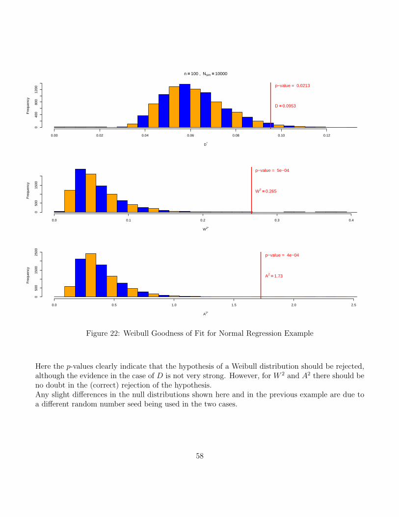
n == 100 , Nsim == 10000
D*
Fre
quen
cy
0.00 0.02 0.04 0.06 0.08 0.10 0.12
040
080
012
00
p−value = 0.0213
D == 0.0953
W2*
Fre
quen
cy
0.0 0.1 0.2 0.3 0.4
050
015
00
p−value = 5e−04
W2 == 0.265
A2*
Fre
quen
cy
0.0 0.5 1.0 1.5 2.0 2.5
050
015
0025
00
p−value = 4e−04
A2 == 1.73
Figure 22: Weibull Goodness of Fit for Normal Regression Example
Here the p-values clearly indicate that the hypothesis of a Weibull distribution should be rejected,although the evidence in the case of D is not very strong. However, for W 2 and A2 there should beno doubt in the (correct) rejection of the hypothesis.Any slight differences in the null distributions shown here and in the previous example are due toa different random number seed being used in the two cases.
58

References
Bain, L.J. (1978) Statistical Analysis of Reliability and Life-Testing Models, New York, Dekker.
Bain, L.J. and Engelhardt M.(1991) Statistical Analysis of Reliability and Life-Testing Models,Theory and Methods, Second Edition, New York, Dekker.
Lawless, J.F. (1982), Statistical Models and Methods for Lifetime Data, John Wiley & Sons, NewYork.
Pierce and Kopecky, K.J. (1979), “Testing Goodness of Fit for the Distribution of Errors in Regres-sion Models,” Biometrika, Vol. 66, No. 1, 1-5
Saunders, S.C. (1975), “Birnbaum’s Contributions to Reliability,” Reliability and Fault Tree Anal-ysis, Theoretical and Applied Aspects of System Reliability and Safety Assessment,Barlow, R.E,Fussell, J.B., and Singpurwalla, N.D. editors, Society for Industrial and Applied Mathematics, 33South 17 Street, Philadelphia PA 19103.
Stephens, M.A. (1986), “Tests based on EDF statistics,” Goodness-of-Fit Techniques, D’Agostino,R. and Stephens, M.A. (editors), Dekker, New York.
Scholz, F.W. (1996) (revised 2001), “Maximum Likelihood Estimation for Type I Censored WeibullData Including Covariates,” ISSTECH-96-022, Boeing Information and Support Services.
Scholz, F.W. (2008) “Weibull Probability Paper,”(informal note).
Thoman, D.R., Bain, L.J., and Antle, C.E. (1969), “Inferences on parameters of the Weibull distri-bution,” Technometrics, Vol 11, No. 3, 445-460.
Thoman, D.R., Bain, L.J., and Antle, C.E. (1970), “Exact confidence intervals for reliability, andtolerance limits in the Weibull distribution,” Technometrics, Vol 12, No. 2, 363-371.
59