Improving Stochastic Policy Gradients in Continuous...

Improving Stochastic Policy Gradients in Continuous Control with DeepReinforcement Learning using the Beta Distribution

Po-Wei Chou 1 Daniel Maturana 1 Sebastian Scherer 1

AbstractRecently, reinforcement learning with deep neu-ral networks has achieved great success in chal-lenging continuous control problems such as 3Dlocomotion and robotic manipulation. However,in real-world control problems, the actions onecan take are bounded by physical constraints,which introduces a bias when the standard Gaus-sian distribution is used as the stochastic policy.In this work, we propose to use the Beta dis-tribution as an alternative and analyze the biasand variance of the policy gradients of both poli-cies. We show that the Beta policy is bias-freeand provides significantly faster convergence andhigher scores over the Gaussian policy whenboth are used with trust region policy optimiza-tion (TRPO) and actor critic with experience re-play (ACER), the state-of-the-art on- and off-policy stochastic methods respectively, on Ope-nAI Gym’s and MuJoCo’s continuous control en-vironments.

1. IntroductionOver the past years, reinforcement learning with deep fea-ture representations (Hinton et al., 2012; Krizhevsky et al.,2012) has achieved unprecedented (or even super-humanlevel) successes in many tasks, including playing Go (Sil-ver et al., 2016) and playing Atari games (Mnih et al., 2013;2015; Guo et al., 2014; Schulman et al., 2015a).

In reinforcement learning tasks, the agent’s action spacemay be discrete, continuous, or some combination of both.Continuous action spaces are generally more challenging(Lillicrap et al., 2015). A naive approach to adapting deepreinforcement learning methods, such as deep Q-learning(Mnih et al., 2013), to continuous domains is simply dis-

1Robotics Institute, Carnegie Mellon University, USA. Correspon-dence to: Sebastian Scherer <[email protected]>.

Proceedings of the 34 th International Conference on MachineLearning, Sydney, Australia, PMLR 70, 2017. Copyright 2017by the author(s).

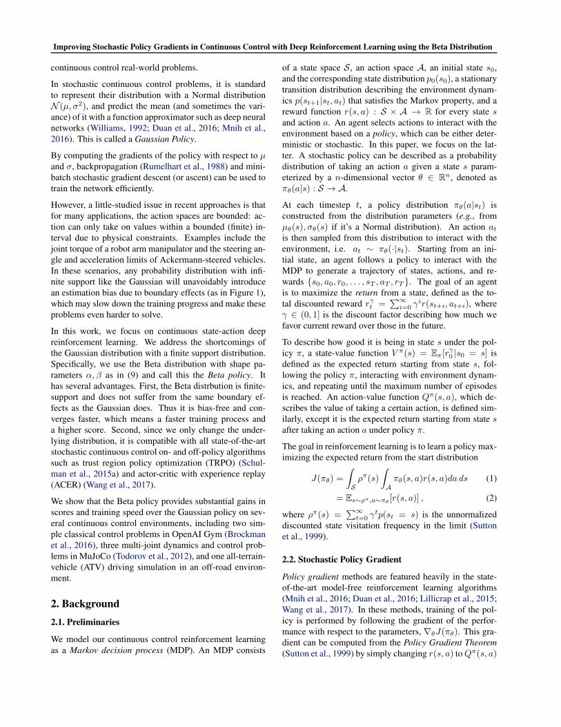
Figure 1. An example of continuous control with bounded actionspace. In most real-world continuous control problems, the ac-tions can only take on values within some bounded interval (finitesupport). For example, the steering angle of most Ackermann-steered vehicles can only range from −30◦ to +30◦.

cretizing the action space. However, this method has sev-eral drawbacks. If the discretization is coarse, the result-ing output will not be smooth; if it is fine, the numberof discretized actions may be intractably high. This issueis compounded in scenarios with high degrees of freedom(e.g., robotic manipulators and humanoid robots), due tothe curse of dimensionality (Bellman, 1956).

There has been much recent progress in model-free contin-uous control with reinforcement learning. AsynchronousAdvantage Actor-Critic (A3C) (Mnih et al., 2016) allowsneural network policies to be trained and updated asyn-chronously with multiple CPU cores in parallel. ValueIteration Networks (Tamar et al., 2016), provide a differ-entiable module that can learn to plan. Exciting resultshave been shown on highly challenging 3D locomotion andmanipulation tasks (Heess et al., 2015; Schulman et al.,2015b;a), including real-world robotics problems wherethe inputs is raw visual data (Watter et al., 2015; Lilli-crap et al., 2015; Levine et al., 2016). Derivative-free blackbox optimization like evolution strategies (Salimans et al.,2017) have also been proven to be very successful in widevariety of tasks.

Despite recent successes, most reinforcement learning al-gorithms still require large amounts of training episodesand huge computational resources. This limits their appli-cability to richer, more complex, and higher dimensional

Improving Stochastic Policy Gradients in Continuous Control with Deep Reinforcement Learning using the Beta Distribution

continuous control real-world problems.

In stochastic continuous control problems, it is standardto represent their distribution with a Normal distributionN (µ,σ2), and predict the mean (and sometimes the vari-ance) of it with a function approximator such as deep neuralnetworks (Williams, 1992; Duan et al., 2016; Mnih et al.,2016). This is called a Gaussian Policy.

By computing the gradients of the policy with respect to µand σ, backpropagation (Rumelhart et al., 1988) and mini-batch stochastic gradient descent (or ascent) can be used totrain the network efficiently.

However, a little-studied issue in recent approaches is thatfor many applications, the action spaces are bounded: ac-tion can only take on values within a bounded (finite) in-terval due to physical constraints. Examples include thejoint torque of a robot arm manipulator and the steering an-gle and acceleration limits of Ackermann-steered vehicles.In these scenarios, any probability distribution with infi-nite support like the Gaussian will unavoidably introducean estimation bias due to boundary effects (as in Figure 1),which may slow down the training progress and make theseproblems even harder to solve.

In this work, we focus on continuous state-action deepreinforcement learning. We address the shortcomings ofthe Gaussian distribution with a finite support distribution.Specifically, we use the Beta distribution with shape pa-rameters α,β as in (9) and call this the Beta policy. Ithas several advantages. First, the Beta distrbution is finite-support and does not suffer from the same boundary ef-fects as the Gaussian does. Thus it is bias-free and con-verges faster, which means a faster training process anda higher score. Second, since we only change the under-lying distribution, it is compatible with all state-of-the-artstochastic continuous control on- and off-policy algorithmssuch as trust region policy optimization (TRPO) (Schul-man et al., 2015a) and actor-critic with experience replay(ACER) (Wang et al., 2017).

We show that the Beta policy provides substantial gains inscores and training speed over the Gaussian policy on sev-eral continuous control environments, including two sim-ple classical control problems in OpenAI Gym (Brockmanet al., 2016), three multi-joint dynamics and control prob-lems in MuJoCo (Todorov et al., 2012), and one all-terrain-vehicle (ATV) driving simulation in an off-road environ-ment.

2. Background2.1. Preliminaries

We model our continuous control reinforcement learningas a Markov decision process (MDP). An MDP consists

of a state space S , an action space A, an initial state s0,and the corresponding state distribution p0(s0), a stationarytransition distribution describing the environment dynam-ics p(st+1|st, at) that satisfies the Markov property, and areward function r(s, a) : S × A → R for every state sand action a. An agent selects actions to interact with theenvironment based on a policy, which can be either deter-ministic or stochastic. In this paper, we focus on the lat-ter. A stochastic policy can be described as a probabilitydistribution of taking an action a given a state s param-eterized by a n-dimensional vector θ ∈ Rn, denoted asπθ(a|s) : S → A.

At each timestep t, a policy distribution πθ(a|st) isconstructed from the distribution parameters (e.g., fromµθ(s),σθ(s) if it’s a Normal distribution). An action atis then sampled from this distribution to interact with theenvironment, i.e. at ∼ πθ(·|st). Starting from an ini-tial state, an agent follows a policy to interact with theMDP to generate a trajectory of states, actions, and re-wards {s0, a0, r0, . . . , sT , aT , rT }. The goal of an agentis to maximize the return from a state, defined as the to-tal discounted reward rγt =

�∞i=0 γ

ir(st+i, at+i), whereγ ∈ (0, 1] is the discount factor describing how much wefavor current reward over those in the future.

To describe how good it is being in state s under the pol-icy π, a state-value function V π(s) = Eπ[r

γ0 |s0 = s] is

defined as the expected return starting from state s, fol-lowing the policy π, interacting with environment dynam-ics, and repeating until the maximum number of episodesis reached. An action-value function Qπ(s, a), which de-scribes the value of taking a certain action, is defined sim-ilarly, except it is the expected return starting from state safter taking an action a under policy π.

The goal in reinforcement learning is to learn a policy max-imizing the expected return from the start distribution

J(πθ) =

�

Sρπ(s)

�

Aπθ(s, a)r(s, a)da ds (1)

= Es∼ρπ,a∼πθ[r(s, a)] , (2)

where ρπ(s) =�∞

t=0 γtp(st = s) is the unnormalized

discounted state visitation frequency in the limit (Suttonet al., 1999).

2.2. Stochastic Policy Gradient

Policy gradient methods are featured heavily in the state-of-the-art model-free reinforcement learning algorithms(Mnih et al., 2016; Duan et al., 2016; Lillicrap et al., 2015;Wang et al., 2017). In these methods, training of the pol-icy is performed by following the gradient of the perfor-mance with respect to the parameters, ∇θJ(πθ). This gra-dient can be computed from the Policy Gradient Theorem(Sutton et al., 1999) by simply changing r(s, a) to Qπ(s, a)


in (2) and moving the gradient operator inside the integral:

∇θJ(πθ) =

�

Sρπ(s)

�

A∇θπθ(a|s)Qπ(s, a)da ds

=

�

Sρπ(s)

�

Aπθ(a|s)gqda ds

= Es∼ρπ,a∼πθ[gq] , (3)

where πθ(a|s) instead of πθ(s, a) is used to represent astochastic policy and gq is the policy gradient estimator us-ing Qπ(s, a) as the target

gq = ∇θ log πθ(a|s)Qπ(s, a) . (4)

However, exact computation of the double integral in (3) isgenerally intractable. Instead, we can estimate it by sam-pling: given enough samples of gq , the sample mean gq ,will converge to its expectation, ∇θJ(πθ), by the law oflarge numbers

gq =1

n

n�

i=1

gqP−→ E[gq] = ∇θJ(πθ), as n → ∞ . (5)

Estimating the policy gradient is one of the most importantissues in reinforcement learning. We want gq in (4) to bebias-free so that it converges to the true policy gradient. Aswe will show in the following section, this is not alwaystrue. At the same time, we also want to reduce the sam-ple variance, so that the gradient is less noisy and stable, asthis improves the convergence rate and speeds up the train-ing progress. The action-value function Qπ(s, a) can beestimated by a variety of sample-based algorithms such asMonte-Carlo (MC) or temporal-difference (TD) learning.A lookup table is usually used to store Qπ(s, a) for eachstate s and action a.

2.3. Stochastic Actor-Critic

For an MDP with intractably large state space, using alookup table is no longer practical. Instead, functionapproximation methods are more common. Deep Q-Networks (DQN) (Mnih et al., 2013) use a deep neural net-work parameterized by θv to approximate the action-valuefunction, denoted as Qθv (s, a) ≈ Qπ(s, a). This is appeal-ing since deep learning has been shown to be very powerfuland successful in computer vision, speech recognition andmany other domains (LeCun et al., 2015).

Unfortunately, direct application of DQN to continuous ac-tion spaces is difficult. First, as mentioned earlier, if wediscretize the action space, it is hampered by the curseof dimensionality. Second, in the Q-learning algorithm,one needs to find the (greedy) action that maximizes theaction-value function, i.e. a = argmaxa Qθv (s, a). Thismeans an additional optimization procedure is required at

every step inside the stochastic gradient descent optimiza-tion, which makes it impractical.

The solution to this is the Actor-Critic methods (Sutton &Barto, 1998; Peters & Schaal, 2008; Degris et al., 2012;Munos et al., 2016). In these methods an actor learns apolicy to select actions and a critic estimates the value func-tion, and criticizes decisions made by the actor. The actorwith policy πθ(a|s) and the critic with Qθv (s, a) are trainedsimultaneously.

Replacing the true action-value function Qπ(s, a) bya function approximator Qθv (s, a) may introduce bias.Nonetheless, in practice, with the help of experience replay(Lin, 1993) and target networks (Mnih et al., 2013) actor-critic methods still converge to good policies, even withdeep neural networks (Lillicrap et al., 2015; Silver et al.,2016).

One of the best known variance reduction technique foractor-critic without introducing any bias is to substract abaseline function B(s) from Qπ(s, a) in (4) (Greensmithet al., 2004). A natural choice for B(s) is V π(s), since it isthe expected action-value function Qπ(s, a), i.e. V π(s) =Ea∼πθ

[Qπ(s, a)]. This gives us the definition of advantagefunction Aπ(s, a) and the following stochastic policy gra-dient estimates:

Aπ(s, a) =Δ Qπ(s, a)− V π(s) , (6)ga = ∇θ log πθ(a|s)Aπ(s, a) . (7)

The advantage function Aπ(s, a) measures how much bet-ter than the average it is to take an action a. With thismethod, the policy gradient in (4) is shifted in a way suchthat it is the relative difference, rather than the absolutevalue Qπ(s, a), that determines the gradient.

3. Infinite/Finite Support Distribution forStochastic Policy in Continuous Control

Using the Gaussian distribution as a stochastic policyin continous control has been well-studied and com-monly used in the reinforcement learning community since(Williams, 1992). This is most likely because the Gaus-sian distribution is easy to sample and has gradients thatare easy to compute, which makes it the first choice of theprobability distribution.

However, we argue that this is not always a good choice.In most continuous control reinforcement learning applica-tions, actions can only take on values within some finite in-terval due to physical constraints, which introduces a non-negligible bias caused by boundary effects, as we show be-low.

This motivates us to use a distribution that can solve thisproblem. Among continuous distributions with finite sup-


-h 0 hAction

Rew

ard

rewardover estimated rewardpolicy distributionbiased policy distribution

biasedtoward

boundary

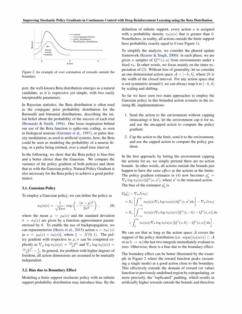
Figure 2. An example of over estimation of rewards outside theboundary.

port, the well-known Beta distribution emerges as a naturalcandidate, as it is expressive yet simple, with two easilyinterpretable parameters.

In Bayesian statistics, the Beta distribution is often usedas the conjugate prior probability distribution for theBernoulli and binomial distributions, describing the ini-tial belief about the probability of the success of each trial(Bernardo & Smith, 1994). One loose inspiration behindour use of the Beta function is spike-rate coding, as seenin biological neurons (Gerstner et al., 1997), or pulse den-sity modulation, as used in artificial systems; here, the Betacould be seen as modeling the probability of a neuron fir-ing, or a pulse being emitted, over a small time interval.

In the following, we show that the Beta policy is bias-freeand a better choice than the Gaussian. We compare thevariance of the policy gradient of both policies and showthat as with the Gaussian policy, Natural Policy Gradient isalso necessary for the Beta policy to achieve a good perfor-mance.

3.1. Gaussian Policy

To employ a Gaussian policy, we can define the policy as

πθ(a|s) =1√2πσ

exp

�− (a− µ)2

2σ2

�, (8)

where the mean µ = µθ(s) and the standard deviationσ = σθ(s) are given by a function approximator param-eterized by θ. To enable the use of backpropagation, wecan reparameterize (Heess et al., 2015) action a ∼ πθ(·|s)as a = µθ(s) + σθ(s)ξ, where ξ ∼ N (0, 1). The pol-icy gradient with respective to µ,σ can be computed ex-plicitly as ∇µ log πθ(a|s) = (a−µ)

σ2 and ∇σ log πθ(a|s) =(a−µ)2

σ3 − 1σ . In general, for problem with higher degrees of

freedom, all action dimensions are assumed to be mutuallyindependent.

3.2. Bias due to Boundary Effect

Modeling a finite support stochastic policy with an infinitesupport probability distribution may introduce bias. By the

definition of infinite support, every action a is assignedwith a probability density πθ(a|s) that is greater than 0.Nonetheless, in reality, all actions outside the finite supporthave probability exactly equal to 0 (see Figure 1).

To simplify the analysis, we consider the phased updateframework (Kearns & Singh, 2000): in each phase, we aregiven n samples of Qπθ (s, a) from environments under afixed πθ. In other words, we focus mainly on the inner ex-pectation of (2). Without loss of generality, let us consideran one-dimensional action space A = [−h, h], where 2h isthe width of the closed interval. For any action space thatis not symmetric around 0, we can always map it to [−h, h]by scaling and shifting.

So far we have seen two main approaches to employ theGaussian policy in this bounded action scenario in the ex-isting RL implementations:

1. Send the action to the environment without capping(truncating) it first, let the environment cap it for us,and use the uncapped action to compute the policygradient.

2. Cap the action to the limit, send it to the environment,and use the capped action to compute the policy gra-dient.

In the first approach, by letting the environment cappingthe actions for us, we simply pretend there are no actionbounds. In other words, all actions outside the bounds justhappen to have the same effect as the actions at the limits.The policy gradient estimator in (4) now becomes g�q =∇θ log πθ(a|s)Qπ(s, a�), where a� is the truncated action.The bias of the estimator g�q is

E[g�q]−∇θJ(πθ)

= Es

�� ∞

−∞πθ(a|s)∇θ log πθ(a|s)Qπ(s, a�)da

�−∇θJ(πθ)

= Es

�� −h

−∞πθ(a|s)∇θ log πθ(a|s) [Qπ(s,−h)−Qπ(s, a)] da

+

� ∞

h

πθ(a|s)∇θ log πθ(a|s) [Qπ(s, h)−Qπ(s, a)] da

�.

We can see that as long as the action space A covers thesupport of the policy distribution (i.e. supp(πθ(a|s)) ⊂ Aor as h → ∞) the last two integrals immediately evaluate tozero. Otherwise, there is a bias due to the boundary effect.

The boundary effect can be better illustrated by the exam-ple in Figure 2 where the reward function peaks (assum-ing a single mode) at a good action close to the boundary.This effectively extends the domain of reward (or value)function to previously undefined region by extrapolating, ormore precisely, the “replicated” padding, which results inartificially higher rewards outside the bounds and therefore


bias the estimated policy distribution toward the boundary.As for multimodal reward functions, one might need toconsider the use of a mixture model or other density es-timation methods since neither the Gaussian nor the Betasuffices under this scenario. However, this is beyond thescope of our discussion.

To make things worse, as σ grows, bias also increases. Thismakes sense intuitively, because as σ grows, more proba-bility density falls outside the boundary. Note that this isnot an unusual case: to encourage the actor to explore thestate space in the early stage of training, larger σ is needed.

In the second approach, the policy gradient estima-tor is even more biased because the truncated actiona� is used both in the state-value function Qπ and inthe gradient of log probability ∇θ log πθ, i.e. g��q =∇θ log πθ(a

�|s)Qπ(s, a�). In this case, the commonlyused variance reduction techique is less useful sinceEa∼πθ

[∇θ log πθ(a�|s)V π(s)] no longer integrates to 0 as

it should be if a instead of a� was used. Not only does itsuffer from the same bias problem we saw earlier, anotherbias is also introduced through the substraction of the base-line function.

3.3. Beta Policy

Let us now consider the Beta distribution

f(x;α,β) =Γ(α+ β)

Γ(α)Γ(β)xα−1(1− x)β−1 , (9)

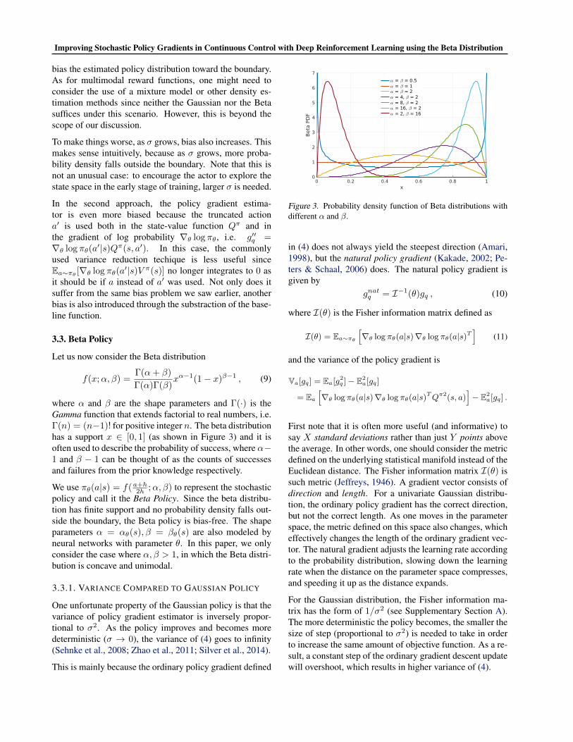
where α and β are the shape parameters and Γ(·) is theGamma function that extends factorial to real numbers, i.e.Γ(n) = (n−1)! for positive integer n. The beta distributionhas a support x ∈ [0, 1] (as shown in Figure 3) and it isoften used to describe the probability of success, where α−1 and β − 1 can be thought of as the counts of successesand failures from the prior knowledge respectively.

We use πθ(a|s) = f(a+h2h ;α,β) to represent the stochastic

policy and call it the Beta Policy. Since the beta distribu-tion has finite support and no probability density falls out-side the boundary, the Beta policy is bias-free. The shapeparameters α = αθ(s),β = βθ(s) are also modeled byneural networks with parameter θ. In this paper, we onlyconsider the case where α,β > 1, in which the Beta distri-bution is concave and unimodal.

3.3.1. VARIANCE COMPARED TO GAUSSIAN POLICY

One unfortunate property of the Gaussian policy is that thevariance of policy gradient estimator is inversely propor-tional to σ2. As the policy improves and becomes moredeterministic (σ → 0), the variance of (4) goes to infinity(Sehnke et al., 2008; Zhao et al., 2011; Silver et al., 2014).

This is mainly because the ordinary policy gradient defined

Figure 3. Probability density function of Beta distributions withdifferent α and β.

in (4) does not always yield the steepest direction (Amari,1998), but the natural policy gradient (Kakade, 2002; Pe-ters & Schaal, 2006) does. The natural policy gradient isgiven by

gnatq = I−1(θ)gq , (10)

where I(θ) is the Fisher information matrix defined as

I(θ) = Ea∼πθ

�∇θ log πθ(a|s)∇θ log πθ(a|s)T

�(11)

and the variance of the policy gradient is

Va[gq] = Ea[g2q ]− E2

a[gq]

= Ea

�∇θ log πθ(a|s)∇θ log πθ(a|s)TQπ2(s, a)

�− E2

a[gq] .

First note that it is often more useful (and informative) tosay X standard deviations rather than just Y points abovethe average. In other words, one should consider the metricdefined on the underlying statistical manifold instead of theEuclidean distance. The Fisher information matrix I(θ) issuch metric (Jeffreys, 1946). A gradient vector consists ofdirection and length. For a univariate Gaussian distribu-tion, the ordinary policy gradient has the correct direction,but not the correct length. As one moves in the parameterspace, the metric defined on this space also changes, whicheffectively changes the length of the ordinary gradient vec-tor. The natural gradient adjusts the learning rate accordingto the probability distribution, slowing down the learningrate when the distance on the parameter space compresses,and speeding it up as the distance expands.

For the Gaussian distribution, the Fisher information ma-trix has the form of 1/σ2 (see Supplementary Section A).The more deterministic the policy becomes, the smaller thesize of step (proportional to σ2) is needed to take in orderto increase the same amount of objective function. As a re-sult, a constant step of the ordinary gradient descent updatewill overshoot, which results in higher variance of (4).


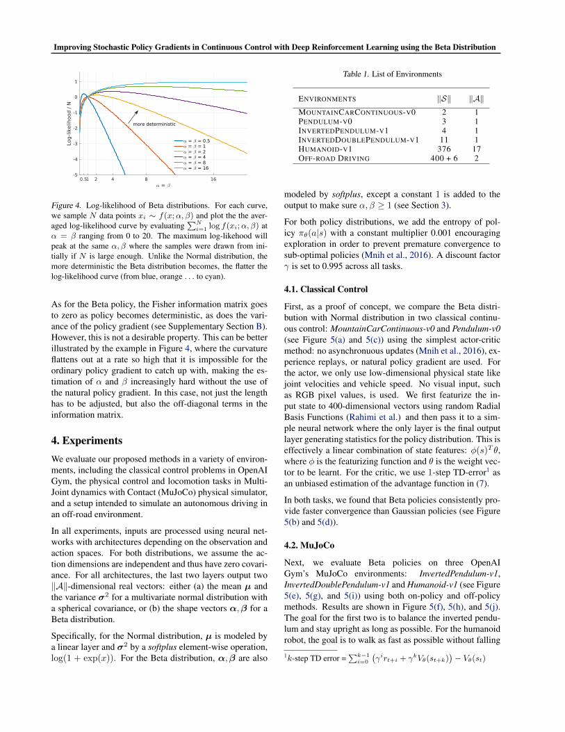
Figure 4. Log-likelihood of Beta distributions. For each curve,we sample N data points xi ∼ f(x;α,β) and plot the the aver-aged log-likelihood curve by evaluating

�Ni=1 log f(xi;α,β) at

α = β ranging from 0 to 20. The maximum log-likehood willpeak at the same α,β where the samples were drawn from ini-tially if N is large enough. Unlike the Normal distribution, themore deterministic the Beta distribution becomes, the flatter thelog-likelihood curve (from blue, orange . . . to cyan).

As for the Beta policy, the Fisher information matrix goesto zero as policy becomes deterministic, as does the vari-ance of the policy gradient (see Supplementary Section B).However, this is not a desirable property. This can be betterillustrated by the example in Figure 4, where the curvatureflattens out at a rate so high that it is impossible for theordinary policy gradient to catch up with, making the es-timation of α and β increasingly hard without the use ofthe natural policy gradient. In this case, not just the lengthhas to be adjusted, but also the off-diagonal terms in theinformation matrix.

4. ExperimentsWe evaluate our proposed methods in a variety of environ-ments, including the classical control problems in OpenAIGym, the physical control and locomotion tasks in Multi-Joint dynamics with Contact (MuJoCo) physical simulator,and a setup intended to simulate an autonomous driving inan off-road environment.

In all experiments, inputs are processed using neural net-works with architectures depending on the observation andaction spaces. For both distributions, we assume the ac-tion dimensions are independent and thus have zero covari-ance. For all architectures, the last two layers output two�A�-dimensional real vectors: either (a) the mean µ andthe variance σ2 for a multivariate normal distribution witha spherical covariance, or (b) the shape vectors α,β for aBeta distribution.

Specifically, for the Normal distribution, µ is modeled bya linear layer and σ2 by a softplus element-wise operation,log(1 + exp(x)). For the Beta distribution, α,β are also

Table 1. List of Environments

ENVIRONMENTS �S� �A�MOUNTAINCARCONTINUOUS-V0 2 1PENDULUM-V0 3 1INVERTEDPENDULUM-V1 4 1INVERTEDDOUBLEPENDULUM-V1 11 1HUMANOID-V1 376 17OFF-ROAD DRIVING 400 + 6 2

modeled by softplus, except a constant 1 is added to theoutput to make sure α,β ≥ 1 (see Section 3).

For both policy distributions, we add the entropy of pol-icy πθ(a|s) with a constant multiplier 0.001 encouragingexploration in order to prevent premature convergence tosub-optimal policies (Mnih et al., 2016). A discount factorγ is set to 0.995 across all tasks.

4.1. Classical Control

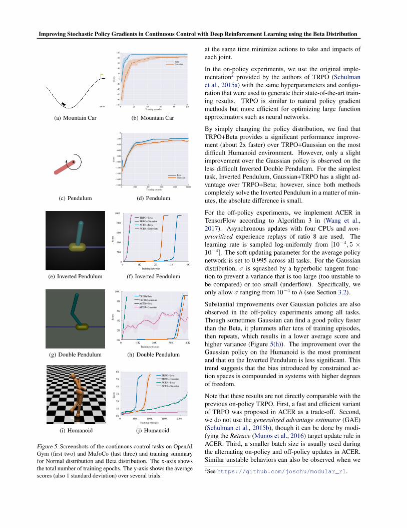
First, as a proof of concept, we compare the Beta distri-bution with Normal distribution in two classical continu-ous control: MountainCarContinuous-v0 and Pendulum-v0(see Figure 5(a) and 5(c)) using the simplest actor-criticmethod: no asynchronuous updates (Mnih et al., 2016), ex-perience replays, or natural policy gradient are used. Forthe actor, we only use low-dimensional physical state likejoint velocities and vehicle speed. No visual input, suchas RGB pixel values, is used. We first featurize the in-put state to 400-dimensional vectors using random RadialBasis Functions (Rahimi et al.) and then pass it to a sim-ple neural network where the only layer is the final outputlayer generating statistics for the policy distribution. This iseffectively a linear combination of state features: φ(s)T θ,where φ is the featurizing function and θ is the weight vec-tor to be learnt. For the critic, we use 1-step TD-error1 asan unbiased estimation of the advantage function in (7).

In both tasks, we found that Beta policies consistently pro-vide faster convergence than Gaussian policies (see Figure5(b) and 5(d)).

4.2. MuJoCo

Next, we evaluate Beta policies on three OpenAIGym’s MuJoCo environments: InvertedPendulum-v1,InvertedDoublePendulum-v1 and Humanoid-v1 (see Figure5(e), 5(g), and 5(i)) using both on-policy and off-policymethods. Results are shown in Figure 5(f), 5(h), and 5(j).The goal for the first two is to balance the inverted pendu-lum and stay upright as long as possible. For the humanoidrobot, the goal is to walk as fast as possible without falling

1k-step TD error =�k−1

i=0

�γirt+i + γkVθ(st+k)

�− Vθ(st)


(a) Mountain Car

Training episodes0 20 40 60 80 100

Scor

e

-100

-80

-60

-40

-20

0

20

40

60

80

100

BetaGaussian

(b) Mountain Car

(c) Pendulum

Training episodes0 200 400 600 800 1000

Scor

e

-1800

-1600

-1400

-1200

-1000

-800

-600

-400

-200

0

BetaGaussian

(d) Pendulum

(e) Inverted Pendulum

0 1K 2K 3K 4K

Training episodes

0

200

400

600

800

1000

Scor

e

TRPO+BetaTRPO+GaussianACER+BetaACER+Gaussian

(f) Inverted Pendulum

(g) Double Pendulum

0 10K 20K 30K 40K

Training episodes

0K

2K

4K

6K

8K

10K

Scor

e


(h) Double Pendulum

(i) Humanoid

0 50K 100K 150K 200K

Training episodes

0K

1K

2K

3K

4K

5K

6K

Scor

e


(j) Humanoid

Figure 5. Screenshots of the continuous control tasks on OpenAIGym (first two) and MuJoCo (last three) and training summaryfor Normal distribution and Beta distribution. The x-axis showsthe total number of training epochs. The y-axis shows the averagescores (also 1 standard deviation) over several trials.

at the same time minimize actions to take and impacts ofeach joint.

In the on-policy experiments, we use the original imple-mentation2 provided by the authors of TRPO (Schulmanet al., 2015a) with the same hyperparameters and configu-ration that were used to generate their state-of-the-art train-ing results. TRPO is similar to natural policy gradientmethods but more efficient for optimizing large functionapproximators such as neural networks.

By simply changing the policy distribution, we find thatTRPO+Beta provides a significant performance improve-ment (about 2x faster) over TRPO+Gaussian on the mostdifficult Humanoid environment. However, only a slightimprovement over the Gaussian policy is observed on theless difficult Inverted Double Pendulum. For the simplesttask, Inverted Pendulum, Gaussian+TRPO has a slight ad-vantage over TRPO+Beta; however, since both methodscompletely solve the Inverted Pendulum in a matter of min-utes, the absolute difference is small.

For the off-policy experiments, we implement ACER inTensorFlow according to Algorithm 3 in (Wang et al.,2017). Asynchronous updates with four CPUs and non-prioritized experience replays of ratio 8 are used. Thelearning rate is sampled log-uniformly from [10−4, 5 ×10−4]. The soft updating parameter for the average policynetwork is set to 0.995 across all tasks. For the Gaussiandistribution, σ is squashed by a hyperbolic tangent func-tion to prevent a variance that is too large (too unstable tobe compared) or too small (underflow). Specifically, weonly allow σ ranging from 10−4 to h (see Section 3.2).

Substantial improvements over Gaussian policies are alsoobserved in the off-policy experiments among all tasks.Though sometimes Gaussian can find a good policy fasterthan the Beta, it plummets after tens of training episodes,then repeats, which results in a lower average score andhigher variance (Figure 5(h)). The improvement over theGaussian policy on the Humanoid is the most prominentand that on the Inverted Pendulum is less significant. Thistrend suggests that the bias introduced by constrained ac-tion spaces is compounded in systems with higher degreesof freedom.

Note that these results are not directly comparable with theprevious on-policy TRPO. First, a fast and efficient variantof TRPO was proposed in ACER as a trade-off. Second,we do not use the generalized advantage estimator (GAE)(Schulman et al., 2015b), though it can be done by modi-fying the Retrace (Munos et al., 2016) target update rule inACER. Third, a smaller batch size is usually used duringthe alternating on-policy and off-policy updates in ACER.Similar unstable behaviors can also be observed when we2See https://github.com/joschu/modular_rl.


(a) Off-Road Driving

0 1K 2K 3K 4K 5K 6KTraining episodes

-20

0

20

40

60

80

100

Scor

e

BetaGaussian

(b) replay ratio 0.25


-20

0

20

40

60

80

100

Scor

e

BetaGaussian

(c) replay ratio 1


-20

0

20

40

60

80

100

Scor

e

BetaGaussian

(d) replay ratio 4

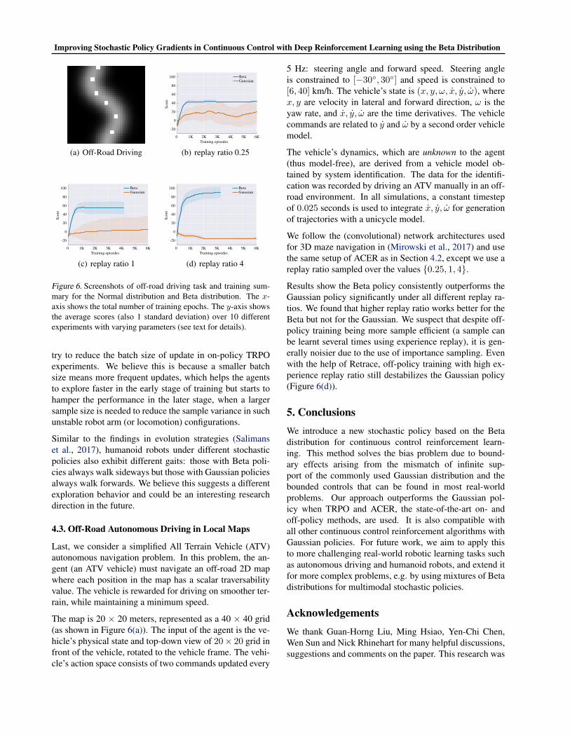
Figure 6. Screenshots of off-road driving task and training sum-mary for the Normal distribution and Beta distribution. The x-axis shows the total number of training epochs. The y-axis showsthe average scores (also 1 standard deviation) over 10 differentexperiments with varying parameters (see text for details).

try to reduce the batch size of update in on-policy TRPOexperiments. We believe this is because a smaller batchsize means more frequent updates, which helps the agentsto explore faster in the early stage of training but starts tohamper the performance in the later stage, when a largersample size is needed to reduce the sample variance in suchunstable robot arm (or locomotion) configurations.

Similar to the findings in evolution strategies (Salimanset al., 2017), humanoid robots under different stochasticpolicies also exhibit different gaits: those with Beta poli-cies always walk sideways but those with Gaussian policiesalways walk forwards. We believe this suggests a differentexploration behavior and could be an interesting researchdirection in the future.

4.3. Off-Road Autonomous Driving in Local Maps

Last, we consider a simplified All Terrain Vehicle (ATV)autonomous navigation problem. In this problem, the an-gent (an ATV vehicle) must navigate an off-road 2D mapwhere each position in the map has a scalar traversabilityvalue. The vehicle is rewarded for driving on smoother ter-rain, while maintaining a minimum speed.

The map is 20 × 20 meters, represented as a 40 × 40 grid(as shown in Figure 6(a)). The input of the agent is the ve-hicle’s physical state and top-down view of 20× 20 grid infront of the vehicle, rotated to the vehicle frame. The vehi-cle’s action space consists of two commands updated every

5 Hz: steering angle and forward speed. Steering angleis constrained to [−30◦, 30◦] and speed is constrained to[6, 40] km/h. The vehicle’s state is (x, y,ω, x, y, ω), wherex, y are velocity in lateral and forward direction, ω is theyaw rate, and x, y, ω are the time derivatives. The vehiclecommands are related to y and ω by a second order vehiclemodel.

The vehicle’s dynamics, which are unknown to the agent(thus model-free), are derived from a vehicle model ob-tained by system identification. The data for the identifi-cation was recorded by driving an ATV manually in an off-road environment. In all simulations, a constant timestepof 0.025 seconds is used to integrate x, y, ω for generationof trajectories with a unicycle model.

We follow the (convolutional) network architectures usedfor 3D maze navigation in (Mirowski et al., 2017) and usethe same setup of ACER as in Section 4.2, except we use areplay ratio sampled over the values {0.25, 1, 4}.

Results show the Beta policy consistently outperforms theGaussian policy significantly under all different replay ra-tios. We found that higher replay ratio works better for theBeta but not for the Gaussian. We suspect that despite off-policy training being more sample efficient (a sample canbe learnt several times using experience replay), it is gen-erally noisier due to the use of importance sampling. Evenwith the help of Retrace, off-policy training with high ex-perience replay ratio still destabilizes the Gaussian policy(Figure 6(d)).

5. ConclusionsWe introduce a new stochastic policy based on the Betadistribution for continuous control reinforcement learn-ing. This method solves the bias problem due to bound-ary effects arising from the mismatch of infinite sup-port of the commonly used Gaussian distribution and thebounded controls that can be found in most real-worldproblems. Our approach outperforms the Gaussian pol-icy when TRPO and ACER, the state-of-the-art on- andoff-policy methods, are used. It is also compatible withall other continuous control reinforcement algorithms withGaussian policies. For future work, we aim to apply thisto more challenging real-world robotic learning tasks suchas autonomous driving and humanoid robots, and extend itfor more complex problems, e.g. by using mixtures of Betadistributions for multimodal stochastic policies.

AcknowledgementsWe thank Guan-Horng Liu, Ming Hsiao, Yen-Chi Chen,Wen Sun and Nick Rhinehart for many helpful discussions,suggestions and comments on the paper. This research was


funded under award by Yamaha Motor Corporation andONR under award N0014-14-1-0643.

ReferencesAmari, Shun-Ichi. Natural gradient works efficiently in

learning. Neural computation, 10(2):251–276, 1998.

Bellman, Richard. Dynamic programming and lagrangemultipliers. Proceedings of the National Academy of Sci-ences, 42(10):767–769, 1956.

Bernardo, J. M. and Smith, A. F. M. Bayesian Theory. JohnWiley & Sons, New York, 1994.

Brockman, Greg, Cheung, Vicki, Pettersson, Ludwig,Schneider, Jonas, Schulman, John, Tang, Jie, andZaremba, Wojciech. Openai gym, 2016.

Degris, Thomas, White, Martha, and Sutton, Richard S.Off-policy actor-critic. arXiv preprint arXiv:1205.4839,2012.

Duan, Yan, Chen, Xi, Houthooft, Rein, Schulman, John,and Abbeel, Pieter. Benchmarking deep reinforcementlearning for continuous control. In Proceedings of The33rd International Conference on Machine Learning,pp. 1329–1338, 2016.

Gerstner, Wulfram, Kreiter, Andreas K., Markram, Henry,and Herz, Andreas V. M. Neural codes: Firing rates and-beyond. Proceedings of the National Academy of Sci-ences, 94(24):12740–12741, 1997.

Greensmith, Evan, Bartlett, Peter L, and Baxter, Jonathan.Variance reduction techniques for gradient estimates inreinforcement learning. Journal of Machine LearningResearch, 5(Nov):1471–1530, 2004.

Guo, Xiaoxiao, Singh, Satinder, Lee, Honglak, Lewis,Richard L, and Wang, Xiaoshi. Deep learning forreal-time atari game play using offline monte-carlo treesearch planning. In Advances in neural information pro-cessing systems, pp. 3338–3346, 2014.

Heess, Nicolas, Wayne, Gregory, Silver, David, Lillicrap,Tim, Erez, Tom, and Tassa, Yuval. Learning continu-ous control policies by stochastic value gradients. In Ad-vances in Neural Information Processing Systems, pp.2944–2952, 2015.

Hinton, Geoffrey, Deng, Li, Yu, Dong, Dahl, George E,Mohamed, Abdel-rahman, Jaitly, Navdeep, Senior, An-drew, Vanhoucke, Vincent, Nguyen, Patrick, Sainath,Tara N, et al. Deep neural networks for acoustic mod-eling in speech recognition: The shared views of fourresearch groups. IEEE Signal Processing Magazine, 29(6):82–97, 2012.

Jeffreys, Harold. An invariant form for the prior probabil-ity in estimation problems. In Proceedings of the RoyalSociety of London a: mathematical, physical and engi-neering sciences, volume 186, pp. 453–461. The RoyalSociety, 1946.

Kakade, Sham M. A natural policy gradient. In Advances inNeural Information Processing Systems, pp. 1531–1538,2002.

Kearns, Michael J and Singh, Satinder P. Bias-variance er-ror bounds for temporal difference updates. In Proceed-ings of the Thirteenth Annual Conference on Compu-tational Learning Theory, pp. 142–147. Morgan Kauf-mann Publishers Inc., 2000.

Krizhevsky, Alex, Sutskever, Ilya, and Hinton, Geoffrey E.Imagenet classification with deep convolutional neuralnetworks. In Advances in neural information processingsystems, pp. 1097–1105, 2012.

LeCun, Yann, Bengio, Yoshua, and Hinton, Geoffrey. Deeplearning. Nature, 521(7553):436–444, 2015.

Levine, Sergey, Finn, Chelsea, Darrell, Trevor, and Abbeel,Pieter. End-to-end training of deep visuomotor poli-cies. The Journal of Machine Learning Research, 17(1):1334–1373, 2016.

Lillicrap, Timothy P, Hunt, Jonathan J, Pritzel, Alexander,Heess, Nicolas, Erez, Tom, Tassa, Yuval, Silver, David,and Wierstra, Daan. Continuous control with deep re-inforcement learning. arXiv preprint arXiv:1509.02971,2015.

Lin, Long-Ji. Reinforcement learning for robots using neu-ral networks. PhD thesis, Fujitsu Laboratories Ltd, 1993.

Mirowski, Piotr, Pascanu, Razvan, Viola, Fabio, Soyer,Hubert, Ballard, Andy, Banino, Andrea, Denil, Misha,Goroshin, Ross, Sifre, Laurent, Kavukcuoglu, Koray,et al. Learning to navigate in complex environments.In The 5th International Conference on Learning Repre-sentations (ICLR), 2017.

Mnih, Volodymyr, Kavukcuoglu, Koray, Silver, David,Graves, Alex, Antonoglou, Ioannis, Wierstra, Daan, andRiedmiller, Martin. Playing atari with deep reinforce-ment learning. In NIPS Deep Learning Workshop, 2013.

Mnih, Volodymyr, Kavukcuoglu, Koray, Silver, David,Rusu, Andrei A, Veness, Joel, Bellemare, Marc G,Graves, Alex, Riedmiller, Martin, Fidjeland, Andreas K,Ostrovski, Georg, et al. Human-level control throughdeep reinforcement learning. Nature, 518(7540):529–533, 2015.


Mnih, Volodymyr, Badia, Adria Puigdomenech, Mirza,Mehdi, Graves, Alex, Lillicrap, Timothy, Harley, Tim,Silver, David, and Kavukcuoglu, Koray. Asynchronousmethods for deep reinforcement learning. In Interna-tional Conference on Machine Learning, pp. 1928–1937,2016.

Munos, Remi, Stepleton, Tom, Harutyunyan, Anna, andBellemare, Marc. Safe and efficient off-policy reinforce-ment learning. In Advances in Neural Information Pro-cessing Systems, pp. 1046–1054, 2016.

Peters, Jan and Schaal, Stefan. Policy gradient methodsfor robotics. In Intelligent Robots and Systems, 2006IEEE/RSJ International Conference on, pp. 2219–2225.IEEE, 2006.

Peters, Jan and Schaal, Stefan. Natural actor-critic. Neuro-computing, 71(7):1180–1190, 2008.

Rahimi, Ali, Recht, Benjamin, et al. Random features forlarge-scale kernel machines.

Rumelhart, David E, Hinton, Geoffrey E, and Williams,Ronald J. Learning representations by back-propagatingerrors. Cognitive modeling, 5(3):1, 1988.

Salimans, Tim, Ho, Jonathan, Chen, Xi, and Sutskever,Ilya. Evolution strategies as a scalable alternative to re-inforcement learning. arXiv preprint arXiv:1703.03864,2017.

Schulman, John, Levine, Sergey, Abbeel, Pieter, Jordan,Michael, and Moritz, Philipp. Trust region policy opti-mization. In Proceedings of The 32nd International Con-ference on Machine Learning, pp. 1889–1897, 2015a.

Schulman, John, Moritz, Philipp, Levine, Sergey, Jordan,Michael, and Abbeel, Pieter. High-dimensional con-tinuous control using generalized advantage estimation.arXiv preprint arXiv:1506.02438, 2015b.

Sehnke, Frank, Osendorfer, Christian, Ruckstieß, Thomas,Graves, Alex, Peters, Jan, and Schmidhuber, Jurgen. Pol-icy gradients with parameter-based exploration for con-trol. In International Conference on Artificial NeuralNetworks, pp. 387–396. Springer, 2008.

Silver, David, Lever, Guy, Heess, Nicolas, Degris, Thomas,Wierstra, Daan, and Riedmiller, Martin. Deterministicpolicy gradient algorithms. In ICML, 2014.

Silver, David, Huang, Aja, Maddison, Chris J, Guez,Arthur, Sifre, Laurent, Van Den Driessche, George,Schrittwieser, Julian, Antonoglou, Ioannis, Panneershel-vam, Veda, Lanctot, Marc, et al. Mastering the game ofgo with deep neural networks and tree search. Nature,529(7587):484–489, 2016.

Sutton, Richard S and Barto, Andrew G. Reinforcementlearning: An introduction, volume 1. MIT press Cam-bridge, 1998.

Sutton, Richard S, McAllester, David A, Singh, Satinder P,Mansour, Yishay, et al. Policy gradient methods for rein-forcement learning with function approximation. 1999.

Tamar, Aviv, Levine, Sergey, Abbeel, Pieter, WU, YI, andThomas, Garrett. Value iteration networks. In Advancesin Neural Information Processing Systems, pp. 2146–2154, 2016.

Todorov, Emanuel, Erez, Tom, and Tassa, Yuval. Mujoco:A physics engine for model-based control. In Intelli-gent Robots and Systems (IROS), 2012 IEEE/RSJ Inter-national Conference on, pp. 5026–5033. IEEE, 2012.

Wang, Ziyu, Bapst, Victor, Heess, Nicolas, Mnih,Volodymyr, Munos, Remi, Kavukcuoglu, Koray, andde Freitas, Nando. Sample efficient actor-critic with ex-perience replay. In The 5th International Conference onLearning Representations (ICLR), 2017.

Wasserman, Larry. All of statistics: a concise course in sta-tistical inference. Springer Science & Business Media,2013.

Watter, Manuel, Springenberg, Jost, Boedecker, Joschka,and Riedmiller, Martin. Embed to control: A locally lin-ear latent dynamics model for control from raw images.In Advances in Neural Information Processing Systems,pp. 2746–2754, 2015.

Williams, Ronald J. Simple statistical gradient-followingalgorithms for connectionist reinforcement learning.Machine learning, 8(3-4):229–256, 1992.

Zhao, Tingting, Hachiya, Hirotaka, Niu, Gang, andSugiyama, Masashi. Analysis and improvement of pol-icy gradient estimation. In Advances in Neural Informa-tion Processing Systems, pp. 262–270, 2011.

Improving Stochastic Policy Gradients in Continuous...

Documents

Transcript of Improving Stochastic Policy Gradients in Continuous...