Improved Estimation and Uncertainty Quantification

Using Monte Carlo-based Optimization Algorithms

Cong Xu, Paul Baines and Jane-Ling Wang

June 16, 2014

Abstract

In this paper we present a novel method to obtain both improved estimates and

reliable stopping rules for stochastic optimization algorithms such as the Monte Carlo

EM (MCEM) algorithm. By characterizing a stationary point, θ∗, of the algorithm as

the solution to a fixed point equation, we provide a parameter estimation procedure

by solving for the fixed point of the update mapping. We investigate various ways to

model the update mapping, including the use of a local linear (regression) smoother.

This simple approach allows increased stability in estimating the value of θ∗ as well

as providing a natural quantification of the estimation uncertainty. These uncertainty

measures can then also be used to construct convergence criteria that reflect the inher-

ent randomness in the algorithm. We establish convergence properties of our modified

estimator. In contrast to existing literature, our convergence results do not require the

Monte Carlo sample size to go to infinity. Simulation studies are provided to illustrate

the improved stability and reliability of our estimator.

Keywords: MCEM algorithm; Stochastic optimization; Local linear smoothing; Stop-

ping rules.

1

1 Introduction

Despite the many advances since its first introduction to the statistical community the EM

algorithm (Dempster et al., 1977) remains one of the most popular optimization algorithms

for both maximum likelihood (ML) and maximum a posterior (MAP) estimation. In many

applications where the EM algorithm is the obvious choice of optimization algorithm the

E-step cannot be computed in closed form. The Monte Carlo EM algorithm, first introduced

by Wei and Tanner (1990), can be used to estimate the required expectations using Monte

Carlo (MC) methods. This approach has been popular in the literature. Notable examples

include McCulloch (1994), McCulloch (1997) and Booth and Hobert (1999). While the

MCEM algorithm allows the EM algorithm to be applied to computationally challenging

problems, the induced randomness leads to two primary challenges for the practitioner:

(i) variability in the optimized value(s), and, (ii) the need to establish reliable stopping

rules/convergence criteria in the presence of MC error. In this paper we present a novel

framework that simultaneously addresses both of these problems for stochastic optimization

algorithms including, but not limited to, MCEM.

There have been a number of proposed modifications of the MCEM algorithm in the

literature to address these issues, including Booth and Hobert (1999), Levine and Casella

(2001) and Caffo et al. (2005). The methods in Booth and Hobert (1999) are based on the

idea of steadily increasing the MC sample size until, to a desired level of confidence, the next

iterate can be distinguished from the previous iterate above and beyond the Monte Carlo

variability. That is, confidence ellipsoids can be formed based upon a normal approximation

to the MC variability, and the MC sample size is then increased whenever subsequent updates

from the algorithm fall within the confidence regions. Levine and Casella (2001) revised the

methods in Booth and Hobert (1999) by recycling the MC samples through importance

weighting to speed up the algorithm. Caffo et al. (2005) propose an Ascent-based MCEM

algorithm that increases the accuracy of the MC approximation to ensure that monotone

convergence is maintained. Both Booth and Hobert (1999) and Caffo et al. (2005) also

2

provide the ability to quantify the Monte Carlo standard error (MCSE) as part of their

approach. Shi and Copas (2002) suggest a much simpler ‘averaging’ approach to address

the issue of variability in the optimized value, combined with some modifications to the

standard convergence criteria. While simpler, the approach of Shi and Copas (2002) does

not always yield optimal results, and requires tuning of the batch size and the lag for the

convergence criteria. We believe that our approach is novel in that it provides a simple way

to address both problems induced by the MC error without requiring an increase in the MC

sample size across iterations. This is achieved by transforming the optimization problem into

an estimation problem that allows both improved estimation and the use of more reliable

stopping rules.

Our approach is based on the simple idea of approximating the update operator in the

neighborhood of a stationary point and obtaining an estimate of the stationary point as

the solution to a fixed point equation. When viewed in this framework, it is clear that

approximating the update operator in the presence of MC error is analogous to estimating

a regression function. The simplest approach is to assume a parametric form for the update

mapping, in which case parametric regression can be applied. For example, approximating

the update operator by a linear function leads to a simple estimate as described in Section 2.2.

However, it will be shown that in general settings, parametric modeling induces a bias in

the estimate. Therefore, we also present a nonparametric regression approach that will

remove the bias in most settings. In this paper, we focus on local linear smoothing (Stone

(1977) and Cleveland (1979)) with the Epanechnikov kernel (Epanechnikov, 1969) which is

optimal as shown by Gasser et al. (1985). The generality of the approach allows us to obtain

reliable uncertainty estimates on the value of θ∗, and to handle multivariate optimization

problems. In all cases our method is simple and fast to implement, and can lead to sizeable

improvements in the reliability of the estimates.

The convergence properties of the MCEM algorithm have been studied by Chan and

Ledolter (1995), Fort and Moulines (2003) and Neath (2012). In particular, Neath (2012)

3

provides a review of convergence results in the presence of MC error. Notably, however,

all existing work establishes convergence of the estimator θ(t) by indefinitely increasing the

Monte Carlo sample size across iterations. In this paper we take an alternative approach

and establish convergence of a modified estimator that does not require the MC sample size

to go to infinity.

The remainder of the paper addresses each of these key points. Section 2 introduces two

modified estimators for stochastic optimization algorithms and establishes their theoretical

properties. A new framework for monitoring convergence is presented in Section 3, while

Section 4 explores the practical performance of our procedures in the context of a simulation

study and a real data example. We conclude with general remarks and possible extensions

in Section 5. Some technical details are deferred to the Appendix.

2 Methodology and Theory

First, consider the case when the parameter of interest is one-dimensional and continuous.

Let θ(t)MC be the parameter estimate from the t-th iteration of a stochastic optimization

algorithm such as MCEM. The one-step-update can be written as

θ(t+1)MC = m(θ

(t)MC) + s(θ

(t)MC)ε

(t)MC , (2.1)

where m(θ(t)MC) is the update of θ

(t)MC that would be obtained if there were no MC error. The

random variable ε(t)MC represents the standardized error in the update with E(ε

(t)MC) = 0 and

V ar(ε(t)MC) = 1. The function s(θ

(t)MC) represents the standard deviation of the stochastic

component of the update, which may depend on θ(t)MC . Typically, s(θ

(t)MC)ε

(t)MC represents

the error attributable to MC approximation. Here we assume that the Monte Carlo or

other stochastic component is designed to have mean zero, with results for non-zero mean

updates provided in section 2.4. In settings where ε(t)MC does indeed represent error from

MC approximation, using CLT-type arguments, it can be natural to make an additional

4

assumption of normality for the MC error, i.e. ε(t)MC ∼ N (0, 1), however we do not require

this. Moreover, the ε(t)MC ’s are naturally independent across iterations whenever independent

Monte Carlo samples are used for each iteration. Note that by accommodating s(·), model

(2.1) is quite flexible as it allows the MC variability to change with θ(t)MC . It is possible

to generalize further to allow for the variance of the error in the update to depend on

additional factors beyond θ(t)MC such as the MC sample size across iterations. For simplicity

of the exposition, however, we assume constant MC sample size at each iteration.

Our goal is to find a stationary point of the optimization algorithm, hopefully corre-

sponding to a global or local maximum of the target function, typically a log-likelihood or

log-posterior distribution. Formally, we want to solve the fixed point equation θ∗ = m(θ∗).

Unfortunately, the update operator m(·) is an unknown function. The idea we adopt here

is to estimate m(·) by md(·) using{θ(0)MC , θ

(1)MC , θ

(2)MC , · · · , θ

(d)MC

}and estimate θ∗ by the cor-

responding fixed point solution of md(·). For simplicity of notation, rewrite (2.1) as

Xt+1 = m(Xt) + s(Xt)εt, (2.2)

withXt = θ(t)MC and εt = ε

(t)MC . Based on (2.2), we observe that the sequence {X0, X1, · · · , Xd}

is a Markov chain and estimating m(·), and the stationary point θ∗, can be viewed as a re-

gression problem based on data points {(X0, X1), (X1, X2), · · · , (Xd−1, Xd)}. As mentioned

in the introduction, two methods are applied to estimate m(·), namely a linear approxima-

tion and a local linear smoother. The two methods are discussed in detail in the following

sections and their long-run convergence properties are provided.

2.1 Convergence of Stochastic Optimization Algorithms

Following Hardle and Tsybakov (1997), we begin by stating some general conditions on m(·),

s(·) and the ε′ts that guarantee stability of the sequence{θ(t)MC : t = 1, 2, . . .

}.

C1. The errors εi’s are i.i.d. and satisfy E(εi) = 0, E(ε2i ) = 1;

5

C2. The function s(x) satisfies that for any compact set X ∈ R, infx∈X

s(x) > 0;

C3. There exist positive constants c1, c2 satisfying c1 + c2E|εi| < 1, such that |m(x)| ≤

c1(1 + |x|) and |s(x)| ≤ c2(1 + |x|);

Conditions C1 and C2 are quite natural while C3 guarantees that the sequence {X0, X1,

· · · , Xd} is non-explosive. In fact, we note that these conditions are only required in some

neighborhood of θ∗ and are generally satisfied in our setting. Under C1-C3, the following

lemma is obtained from the results of Nummelin and Tuominen (1982).

Lemma 1. Under C1-C3 the Markov chain {X0, X1, · · · , Xd} is geometrically ergodic, which

means it is ergodic with stationary probability measure Pπ satisfying that for almost every x,

‖Pt(·|x)− Pπ(·)‖TV = O(ρt),

for some 0 ≤ ρ < 1, where Pt(B|x) = P (Xt ∈ B|X0 = x) for any Borel subset B ⊂ R and

‖ · ‖TV represents the total variation.

The proof is given in Nummelin and Tuominen (1982). Lemma 1 establishes the long-run

stability of {X0, X1, . . . , Xd}. In addition to C1-C3, two additional conditions are needed to

prove the theoretical properties of our estimators.

C4. For the stationary probability measure Pπ in Lemma 1, the density π(·) of Pπ exists and

is bounded, continuous and strictly positive in a neighborhood of θ∗. In addition, for

X ∼ π(·), E|X|2+δ <∞ for some constant δ > 0;

C5. Function m(·) is twice differentiable with m′′(·) being bounded and Lipschitz continuous.

Moreover, m′(·) is bounded away from 1 in a neighborhood of θ∗.

Under these general conditions, we now investigate two methods to estimate m(·), and thus

the stationary point θ∗.

6

2.2 Linear Approximation of the Update Map

In this section, we consider the simple idea of approximatingm(·) in (2.1) by a linear function.

This simple idea is nonetheless supported by the observation that the underlying update

operator m(·) is approximately linear in a small neighborhood of θ∗. While the true update

mapping m(·) can be non-linear, the linear approximation framework is based on modeling

θ(t+1)MC = β0 + θ

(t)MCβ1 + σε

(t)MC . (2.3)

Let mLRt (x) = β

(t)0 + β

(t)1 x denote the linear regression-based estimate of m(x), then θ

(t)LR, the

estimated stationary point of mLRt (x), is seen to be

θ(t)LR =

β(t)0

1− β(t)1

. (2.4)

Note that for simplicity here we additionally assume in (2.3) that the MC error has con-

stant variance so the coefficients (β(t)0 and β

(t)1 ) can be obtained by ordinary least squares

based on the data points {(X0, X1), (X1, X2), · · · , (Xt−1, Xt)}. This is a natural assumption

when the MC sample size is constant. Generalizations to allow for non-constant variance

can be achieved by modifying the estimates of (β(t)0 , β

(t)1 ) correspondingly, e.g. weighted

least square estimates. This simple and fast procedure allows the user to utilize the entire

sequence{θ(1)MC , θ

(2)MC , . . . , θ

(t)MC

}, possibly after discarding an initial ‘burn-in’, to estimate the

stationary point at iteration t, rather than using θ(t)MC only. In practice, it can be beneficial

to discard an initial set of I iterations and to wait t0 iterations before using this procedure.

An algorithm for finding a stationary point of a stochastic optimization algorithm using this

linear approximation to the update operator is given below.

1. Let t = 0. Select a starting value θ(0)MC ;

2. Obtain θ(t+1)MC from a single iteration of the optimization algorithm starting at θ

(t)MC ;

3. If t > t0, obtain θ(t)LR using (2.4) based on {θ(I)MC , θ

(I+1)MC , · · · , θ(t)MC};

7

4. Check for convergence; If converged, estimate θ∗ with θ(t)LR, else continue to step 5;

5. Increment t 7→ t+ 1 and return to step 2.

The choice of stopping rule in step 4 is also of interest, and is discussed in Section 3. The

long-run properties of θ(t)LR are given in the theorem below. In contrast to Neath (2012), Booth

and Hobert (1999) and Caffo et al. (2005), we examine the behavior of θ(t)LR as t → ∞ with

non-vanishing MC error, thus not requiring the MC sample size to increase indefinitely.

Theorem 1. Assume that C1-C5 hold and θ∗ is an isolated stationary point of m(x), i.e.

θ∗ is the unique stationary point in a neighborhood (a, b) containing θ∗. Moreover, assume

that m(x) is smooth in (a, b). Then the linear regression-based estimator θ(t)LR satisfies

θ(t)LR

a.s.−−→ θ∗ +

∞∑k=2

m(k)(θ∗)Eπ(X − θ∗)k/k!

1−m′(θ∗)= Eπ(X), (2.5)

|θ(t)LR − Eπ(X)| = Op

(1√t

), (2.6)

where Eπ(·) stands for the expectation w.r.t. density π(·) in C4 and m(k)(·) represents the

k-th derivative of m(·).

Theorem 1 demonstrates that θ(t)LR is a biased estimator of θ∗ unless m(x) is exactly linear

(i.e. m(k)(x) ≡ 0, for k = 2, 3, · · · so that the bias term in (2.5) vanishes). In practice, θ(t)LR

can be a fairly good estimator when the bias term is negligible, as occurs when the Monte

Carlo errors are small in a relative sense. However, the induced bias can be non-negligible in

situations where the MC error cannot be minimized due to computational restrictions. The

primary gain however, as will be demonstrated in Section 4, is that the variance of θ(t)LR is

drastically smaller than the variance of θ(t)MC or other ‘look-back’ averages. Indeed, as shown

in (2.6), even with non-vanishing MC variance, the variance of θ(t)LR goes to zero. This is in

contrast to θ(t)MC , which fails to converge, and a last-ten average (Shi and Copas, 2002), that

has a non-zero long-run variance. These gains are simply attained by using the full sample

8

path{θ(I)MC , θ

(I+1)MC , . . . , θ

(d)MC

}to estimate θ∗, rather than the last, or last-10 iterations only.

While a linear-approximation may suffice for many problems, it is simple to generalize in

such a manner that we can remove the bias in (2.5) in fairly wide generality using the local

linear smoothing approach in Section 2.3. We conclude by noting that for multi-parameter

problems, both the linear regression and local linear smoothing procedures can be applied

to each parameter separately. In these settings the update in (2.1) is applied to the full

parameter, with the fixed point estimation and accompanying uncertainty quantification

performed marginally for each parameter. Since the stochastic update is performed in the

joint space, the vector of marginal fixed points is a fixed point for the full parameter vector.

2.3 Local Linear Smoothing

In this section we define and establish the basic properties of the local linear smoothing-based

estimate. Let ht be the bandwidth and K(·) be the kernel function, denote uit = Xi−1−xht

and

Uit = (1, uit)T . The local linear smoother at(x) = (at0(x), at1(x))T is then defined as

at(x) = argmina∈R2

t∑i=1

(Xi − aTUit

)2K(uit). (2.7)

In the following, we establish the asymptotic properties of θ(t)LS (the quasi-fixed point or

quasi-stationary point corresponding to mLSt (x) = at0(x) defined below in Theorem 2). To

distinguish between the linear approximation-based estimators of Section 2.2 we use the

superscript “LS” for both mLSt (x) and θ

(t)LS to denote the local linear smoothing-based es-

timator. In addition to C1-C5, some additional conditions are required to establish the

asymptotic properties for the local linear smoothing-based estimate:

C6. The function K(·) is a strictly positive and bounded function with compact support;

C7. The bandwidth ht = O{(

log tt

) 15

}.

9

In the examples of Section 4 the Epanechnikov kernel, K(u) = 34(1 − u2)I(|u| ≤ 1), is used

so that C6 is readily satisfied. The following results follow from Theorem 6 of Masry (1996)

and states the asymptotic properties of θ(t)LS.

Theorem 2. Assume that C1-C7 holds and θ∗ is an isolated stationary point of m(x), i.e.

θ∗ is the unique stationary point in a neighborhood (a, b) containing θ∗. Then when t is large

enough, there exists θ(t)LS ∈ (a, b), a quasi-stationary point of mLS

t (x), satisfying

θ(t)LS

a.s.−−→ θ∗, (2.8)

|θ(t)LS − θ∗| = O

{(log t

t

) 25

}a.s., (2.9)

with quasi-stationary points of mLSt (x) defined as those x such that |mLS

t (x)−x| = O{(

log tt

) 25

}.

Theorem 2 assures that θ(t)LS is a consistent estimate of θ∗ under the conditions listed above.

The quasi-stationary points of mLSt (x) may not be unique in (a, b) and we could choose one

of them as θ(t)LS. Note that we are not using the exact fixed point of mLS

t (x) which is hard

to obtain in practice due to the difficulty of solving the nonlinear equation mLSt (x) = x.

What we do in practice is to evaluate mLSt (x) at a dense grid of (a, b) and pick one satisfying

|mLSt (x) − x| ≤ C0

(log tt

) 25 for some constant C0 > 0.Theorem 2 guarantees that doing this

would not harm the asymptotic properties of our local linear smoothing procedure. Our local

linear smoothing algorithm mirrors that of Section 2.2 with θ(t)LS replacing θ

(t)LR. The result

in (2.8) is, to our best knowledge, the first result establishing the long-run consistency of a

stochastic optimization algorithm for non-linear update mappings that does not require the

MC variance to go to zero. As such, it provides the user with basic theoretical assurances

without needing to increase the MC sample size (or decrease the MC error) indefinitely.

10

2.4 Estimation with Non-Zero Mean Stochastic Updates

The convergence results of the previous sections are restricted to settings where the stochastic

update mapping is unbiased i.e., E[θ(t+1)MC |θ

(t)MC

]= m(θ

(t)MC). In some contexts it may not be

feasible to construct a stochastic update that has this property, and instead a biased update

may be used. We now extend (2.1) to

θ(t+1)MC = m(θ

(t)MC) + ε

(t)MC , (2.10)

E[ε(t)MC |θ

(t)MC

]= bk(t)(θ

(t)MC), Var

(ε(t)MC |θ

(t)MC

)= sk(t)(θ

(t)MC),

where bk(t)(θ(t)MC) is the bias of the stochastic update as a function of the current state of

the algorithm. Here the term ‘bias’ refers exclusively to the expected discrepancy between

the stochastic update and the deterministic update that would be obtained without Monte

Carlo error, and not to the bias of the estimator of θ. We let the bias and variance explicitly

depend on a value k that controls the accuracy of the stochastic update, with larger values of

k corresponding to ‘more accurate’ updates. Typically k would correspond to the MC sample

size (or a tuning parameter controlling the error in the stochastic update), which can vary

with the iteration number t i.e., k(t) could represent the MC sample size used at iteration t.

We assume k(t) is a non-decreasing function of t. This generality is introduced to allow for

us to study the behavior of estimators when the stochastic error can be made to vanish. As

can be seen from (2.10), the bias term will be absorbed into the update function, and thus

(subject to additional regularity conditions discussed shortly) the sequence{θ(0)MC , θ

(1)MC , . . .

}will converge to a fixed point of the function m(θ) = m(θ) + b(θ). In general, the fixed point

of m is not a fixed point of m unless b(θ∗) = 0 i.e., the bias vanishes at the fixed point.

In the following we consider the behavior of estimators of θ under two conditions: (i)

when limt→∞

bk(t)(θ∗) 6= 0, and, (ii) when lim

t→∞bk(t)(θ

∗) = 0. Setting (i) corresponds to a setting

with non-vanishing bias in the stochastic update, whereas (ii) corresponds to the setting

where the stochastic error vanishes as the tuning parameter controlling the accuracy of the

11

stochastic update is increased. For example, (ii) would apply to a setting where the update

is biased, but the bias goes to zero as the MC sample size goes to infinity.

First, we address setting (i), where the bias in the stochastic update does not vanish.

Under these conditions, estimators produced using the regular MCEM algorithm, the algo-

rithm of Caffo et al. (2005), and our estimators proposed in Section 2.2 and 2.3 in general

do not converge to a stationary point of the target function. Indeed, as may be expected, no

method that does not explicitly correct for the bias will converge to the correct stationary

point. For example, consider the simple case of a linear update function, m(θ) = a + bθ,

with linear bias, b(θ) = a+ bθ. In this case the fixed point becomes:

θ∗ =a+ a

1− (b+ b),

which will in general differ from the desired stationary point θ∗ = a/(1− b). In cases when

the bias is small, for practical purposes the converged value may not differ much from the

desired stationary point. The convergence results of Section 2.2 and 2.3 can be seen to hold

directly with the conditions on m replaced by identical conditions on the modified update

operator m. It is worth noting, however, that if the bias can be estimated and corrected

for then the approaches presented here and in Caffo et al. (2005) may be applied to the

corrected updates, which will then converge to the desired stationary point(s).

The second setting, where limt→∞ bk(t)(θ∗) = 0 can be understood similarly. In this case,

algorithms that let k → ∞ will (under the standard regularity conditions) converge to θ∗,

a stationary point of the target function. In contrast, our methodology is designed to run

with fixed precision k (e.g., non-increasing Monte Carlo sample size), and thus the bias will

not vanish. In this context the estimators proposed in sections 2.2 and 2.3 will converge

to a fixed point of m instead of a fixed point of m. In practice the bias of the resulting

estimator will often be very small if the bias in the update is small or the convergence rate

of the algorithm is low (i.e., fast convergence, small b). However, in cases where an unbiased

12

stochastic update cannot be designed and the bias in the stochastic update is large for finite

k but vanishes as k → ∞, procedures based on increasing the accuracy of the stochastic

update, such as Caffo et al. (2005) may be preferred. Section 4 provides an example with

non-zero but vanishing bias in the stochastic update to illustrate these trade-offs.

3 Convergence Criteria

We now address the second of the challenges of using a stochastic optimization algorithm

such as MCEM: reliably monitoring convergence. For non-stochastic optimization algorithms

it is typical to use absolute or relative error criteria of the form:

‖θ(t+1) − θ(t)‖ < c, or ,‖θ(t+1) − θ(t)‖‖θ(t)‖

< c, (3.1)

where c is a small positive constant. Unfortunately, for stochastic algorithms, since θ(t)MC

in (2.1) is a random variable, there is a non-negligible probability that the criteria in (3.1) will

be satisfied even if θ(t)MC is not close to a local (or global) mode. In addition, if the constant c

is chosen to be very small to minimize the probability of an early-stoppage, then it is possible

that the algorithm may not converge in reasonable time. In either case, using deterministic

criteria such as those in (3.1) requires very careful problem-specific tuning of c to match the

inherent level of stochastic variability and is not practical in most settings. These problems

are noted in Booth and Hobert (1999), who propose various schemes to achieve more robust

stopping rules based on increasing the sample size according to confidence ellipsoids around

the parameter values. This scheme is more effective but introduces more of a programming

burden, and requires increasing MC sample size across iterations.

In practice, as shown in the simulation of Section 4.1, the problem of using deterministic

stopping rules is somewhat alleviated when using our modified estimates introduced in Sec-

tion 2 due to their increased stability. However, despite reasonable practical performance in

many settings, such an approach still does not properly account for the randomness in the

13

sequence. To address these limitations, we now propose an alternative method to reliably

monitor convergence of stochastic optimization algorithms of the form (2.1) without increas-

ing the MC sample size. Using the sample path of the algorithm {θ(0)MC , θ(1)MC , . . . , θ

(t)MC} we

obtain pairs {(θ(j+1)MC , θ

(j)MC) : j = 0, . . . , t − 1} corresponding to observations of the update

operator m(·) with conditionally independent errors that correspond to the MC variability.

In using an estimate, say θ(t)LS, of the stationary point as an estimate of θ∗, we can also use the

uncertainty or standard error of θ(t)LS attributable to MC variability to monitor convergence.

Note that here, when we refer to the uncertainty in θ(t)LS attributable to MC variability, we

are referring only to uncertainty induced by ε(t)MC in (2.1). We define this to be the Monte

Carlo SE, distinct from the usual SE of the estimate attributable to the data/model. For

vanilla EM, or non-stochastic algorithms, the MCSE will be zero; for stochastic algorithms

it reflects the additional uncertainty in estimation due to the MC variability.

The idea to use the MCSE to monitor convergence is simple and has been used many

times before. Examples include Booth and Hobert (1999) and Caffo et al. (2005). Once

the MCSE, or some function of the MCSE, falls below a chosen threshold, the algorithm

is declared to have converged. This MCSE check should be combined with a check on the

absolute or relative tolerance of estimates at successive iterations to avoid cases where the

MCSE falls below the threshold while the algorithm is still climbing toward the stationary

point. Therefore, in all cases we additionally check that the relative tolerance between

successive iterations falls below the same threshold as the MCSE. The key for our context

is how to estimate the MCSE at iteration t, for which we propose the following bootstrap

procedure:

1. Set b = 1;

2. Take a bootstrap sample S(t)b of size t from S(t) = {(θ(j+1)

MC , θ(j)MC) : j = 0, . . . , t− 1} i.e.,

sample t pairs (θ(j+1)MC , θ

(j)MC) with replacement from S(t);

3. Obtain θ(t)b , an estimate of the stationary point for the bootstrapped sample, i.e., we

14

obtain θ(t)LR or θ

(t)LS based on S

(t)b ;

4. If b = B, stop, else increment b 7→ b+ 1 and return to Step 2.

The resulting sample {θ(t)b : b = 1, . . . , B} can be used to estimate the standard deviation

of θ(t). If this falls below the desired threshold and successive iterates are ‘close’, then the

algorithm is declared to have converged. While the above procedure minimizes the chance

of an incorrect early-stoppage, and can be applied to any estimate of the stationary point, it

can potentially be slow as the number of iterations is large. Therefore, in situations where

speed is a primary concern, we recommend applying this procedure as an additional criterion

to check convergence only after simpler criteria such as those in (3.1) have been satisfied.

This strategy provides a compromise between the use of reliable criteria and speed, since it

avoids running the bootstrap procedure at each iteration.

4 Simulation and Application

4.1 Example I: Genetic Linkage Model

Our first example is the genetic linkage model described in Dempster et al. (1977) and Wei

and Tanner (1990). This is an example where the EM-update operator has an explicit form

and applying MCEM is actually not necessary. However, this serves as a good example

which allows us to add an artificial error term to mimic Monte Carlo error and examine the

performance of the proposed procedure in Section 2. Details are provided below.

The data consists of n = 197 animals which are multinomially distributed into four cat-

egories. The observed data is y = (y1, y2, y3, y4) = (125, 18, 20, 34) and the cell probabilities

are given by(12

+ θ4, 1−θ

4, 1−θ

4, θ4

). To apply the EM algorithm, the first of the four original cat-

egories is split into two categories and the complete data is denoted by x = (x1, x2, x3, x4, x5)

with cell probabilities(12, θ4, 1−θ

4, 1−θ

4, θ4

)where y1 = x1 + x2, y2 = x3, y3 = x4 and y4 = x5.

15

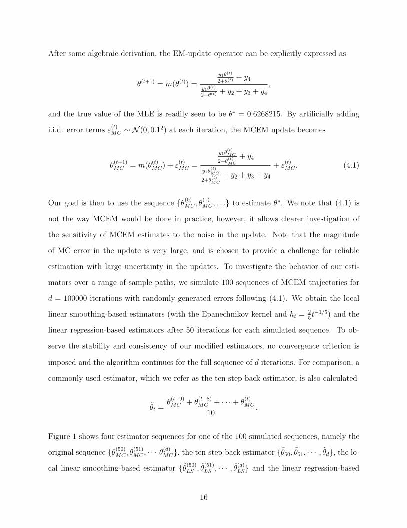
After some algebraic derivation, the EM-update operator can be explicitly expressed as

θ(t+1) = m(θ(t)) =

y1θ(t)

2+θ(t)+ y4

y1θ(t)

2+θ(t)+ y2 + y3 + y4

,

and the true value of the MLE is readily seen to be θ∗ = 0.6268215. By artificially adding

i.i.d. error terms ε(t)MC ∼ N (0, 0.12) at each iteration, the MCEM update becomes

θ(t+1)MC = m(θ

(t)MC) + ε

(t)MC =

y1θ(t)MC

2+θ(t)MC

+ y4

y1θ(t)MC

2+θ(t)MC

+ y2 + y3 + y4

+ ε(t)MC . (4.1)

Our goal is then to use the sequence {θ(0)MC , θ(1)MC , . . .} to estimate θ∗. We note that (4.1) is

not the way MCEM would be done in practice, however, it allows clearer investigation of

the sensitivity of MCEM estimates to the noise in the update. Note that the magnitude

of MC error in the update is very large, and is chosen to provide a challenge for reliable

estimation with large uncertainty in the updates. To investigate the behavior of our esti-

mators over a range of sample paths, we simulate 100 sequences of MCEM trajectories for

d = 100000 iterations with randomly generated errors following (4.1). We obtain the local

linear smoothing-based estimators (with the Epanechnikov kernel and ht = 25t−1/5) and the

linear regression-based estimators after 50 iterations for each simulated sequence. To ob-

serve the stability and consistency of our modified estimators, no convergence criterion is

imposed and the algorithm continues for the full sequence of d iterations. For comparison, a

commonly used estimator, which we refer as the ten-step-back estimator, is also calculated

θt =θ(t−9)MC + θ

(t−8)MC + · · ·+ θ

(t)MC

10.

Figure 1 shows four estimator sequences for one of the 100 simulated sequences, namely the

original sequence {θ(50)MC , θ(51)MC , · · · θ

(d)MC}, the ten-step-back estimator {θ50, θ51, · · · , θd}, the lo-

cal linear smoothing-based estimator {θ(50)LS , θ(51)LS , · · · , θ

(d)LS} and the linear regression-based

16

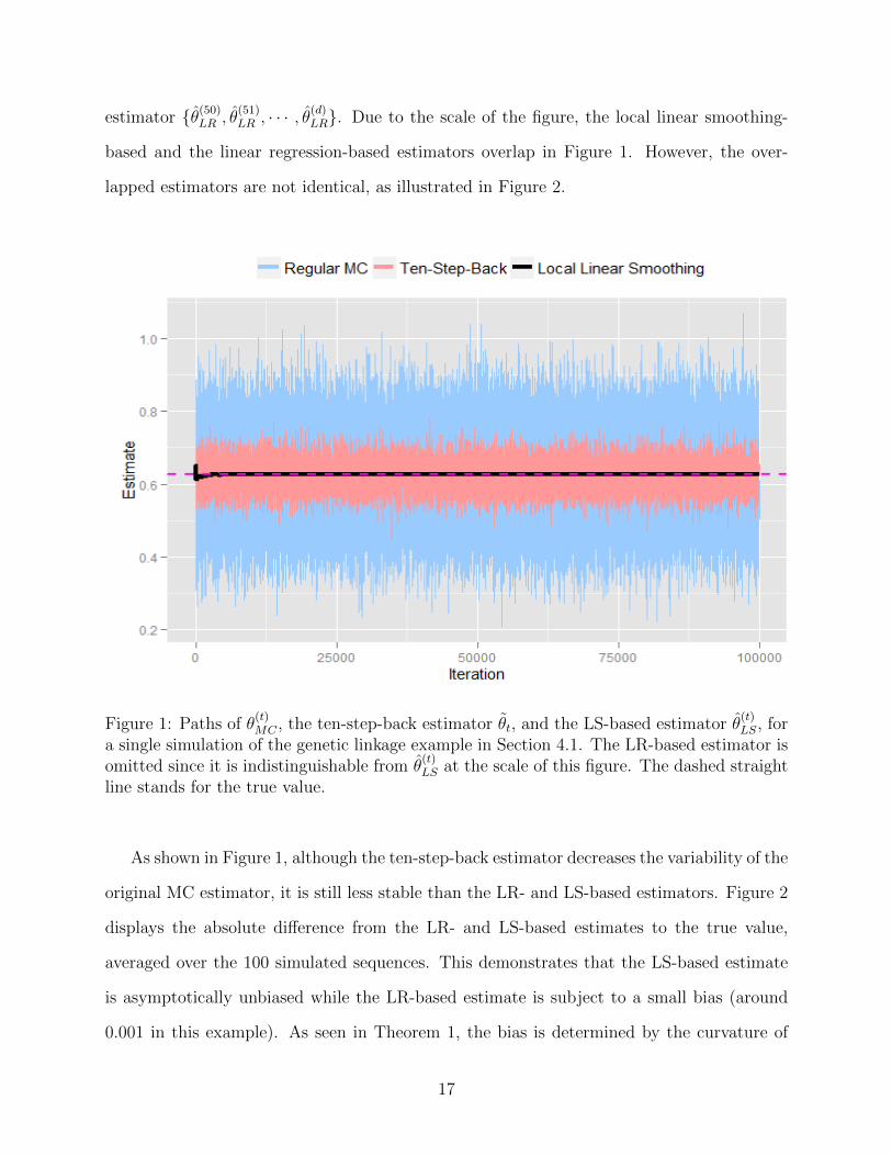
estimator {θ(50)LR , θ(51)LR , · · · , θ

(d)LR}. Due to the scale of the figure, the local linear smoothing-

based and the linear regression-based estimators overlap in Figure 1. However, the over-

lapped estimators are not identical, as illustrated in Figure 2.

Figure 1: Paths of θ(t)MC , the ten-step-back estimator θt, and the LS-based estimator θ

(t)LS, for

a single simulation of the genetic linkage example in Section 4.1. The LR-based estimator isomitted since it is indistinguishable from θ

(t)LS at the scale of this figure. The dashed straight

line stands for the true value.

As shown in Figure 1, although the ten-step-back estimator decreases the variability of the

original MC estimator, it is still less stable than the LR- and LS-based estimators. Figure 2

displays the absolute difference from the LR- and LS-based estimates to the true value,

averaged over the 100 simulated sequences. This demonstrates that the LS-based estimate

is asymptotically unbiased while the LR-based estimate is subject to a small bias (around

0.001 in this example). As seen in Theorem 1, the bias is determined by the curvature of

17

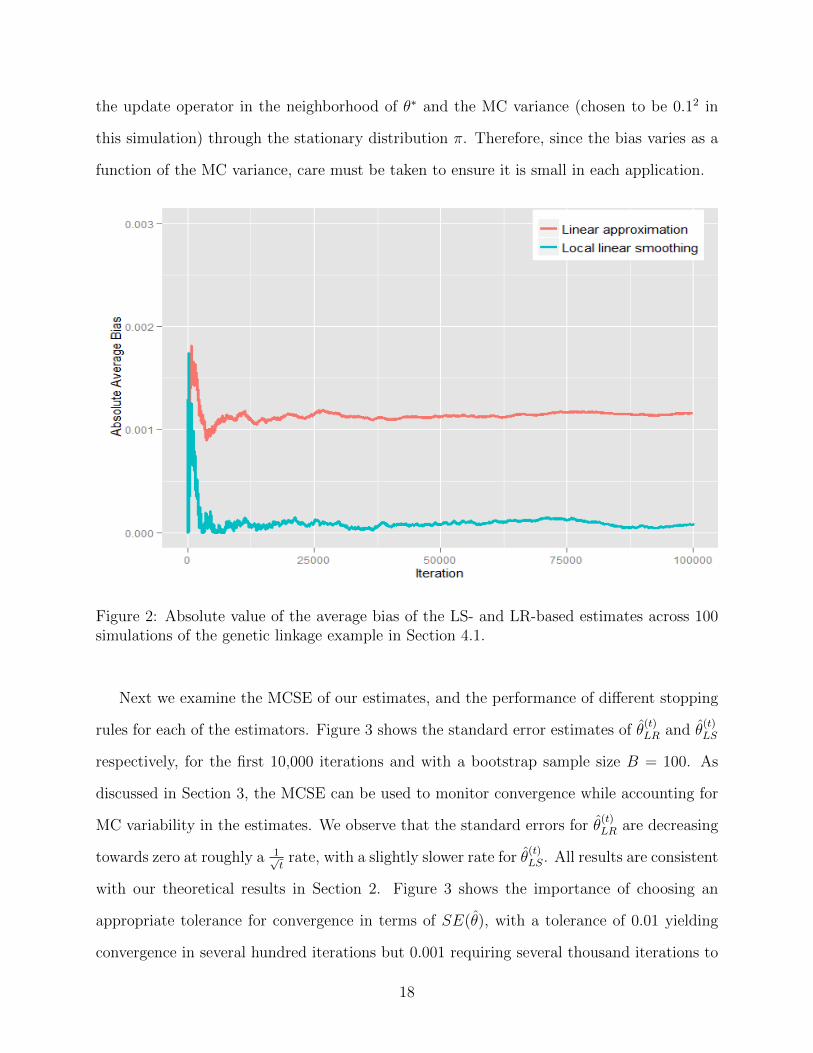
the update operator in the neighborhood of θ∗ and the MC variance (chosen to be 0.12 in

this simulation) through the stationary distribution π. Therefore, since the bias varies as a

function of the MC variance, care must be taken to ensure it is small in each application.

Figure 2: Absolute value of the average bias of the LS- and LR-based estimates across 100simulations of the genetic linkage example in Section 4.1.

Next we examine the MCSE of our estimates, and the performance of different stopping

rules for each of the estimators. Figure 3 shows the standard error estimates of θ(t)LR and θ

(t)LS

respectively, for the first 10,000 iterations and with a bootstrap sample size B = 100. As

discussed in Section 3, the MCSE can be used to monitor convergence while accounting for

MC variability in the estimates. We observe that the standard errors for θ(t)LR are decreasing

towards zero at roughly a 1√t

rate, with a slightly slower rate for θ(t)LS. All results are consistent

with our theoretical results in Section 2. Figure 3 shows the importance of choosing an

appropriate tolerance for convergence in terms of SE(θ), with a tolerance of 0.01 yielding

convergence in several hundred iterations but 0.001 requiring several thousand iterations to

18

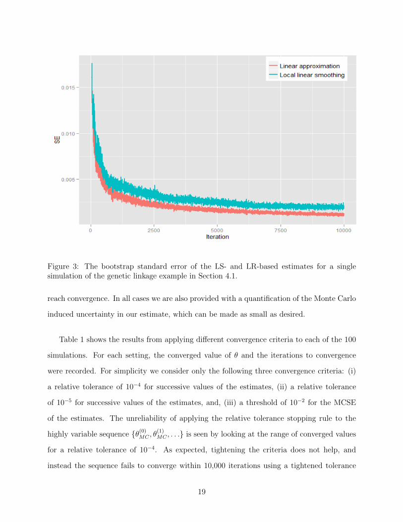
Figure 3: The bootstrap standard error of the LS- and LR-based estimates for a singlesimulation of the genetic linkage example in Section 4.1.

reach convergence. In all cases we are also provided with a quantification of the Monte Carlo

induced uncertainty in our estimate, which can be made as small as desired.

Table 1 shows the results from applying different convergence criteria to each of the 100

simulations. For each setting, the converged value of θ and the iterations to convergence

were recorded. For simplicity we consider only the following three convergence criteria: (i)

a relative tolerance of 10−4 for successive values of the estimates, (ii) a relative tolerance

of 10−5 for successive values of the estimates, and, (iii) a threshold of 10−2 for the MCSE

of the estimates. The unreliability of applying the relative tolerance stopping rule to the

highly variable sequence {θ(0)MC , θ(1)MC , . . .} is seen by looking at the range of converged values

for a relative tolerance of 10−4. As expected, tightening the criteria does not help, and

instead the sequence fails to converge within 10,000 iterations using a tightened tolerance

19

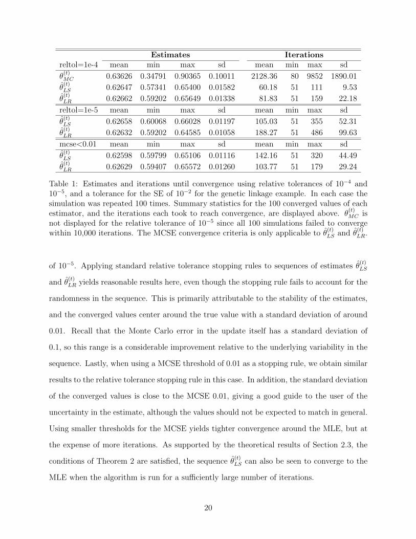
Estimates Iterationsreltol=1e-4 mean min max sd mean min max sd

θ(t)MC 0.63626 0.34791 0.90365 0.10011 2128.36 80 9852 1890.01

θ(t)LS 0.62647 0.57341 0.65400 0.01582 60.18 51 111 9.53

θ(t)LR 0.62662 0.59202 0.65649 0.01338 81.83 51 159 22.18

reltol=1e-5 mean min max sd mean min max sd

θ(t)LS 0.62658 0.60068 0.66028 0.01197 105.03 51 355 52.31

θ(t)LR 0.62632 0.59202 0.64585 0.01058 188.27 51 486 99.63

mcse<0.01 mean min max sd mean min max sd

θ(t)LS 0.62598 0.59799 0.65106 0.01116 142.16 51 320 44.49

θ(t)LR 0.62629 0.59407 0.65572 0.01260 103.77 51 179 29.24

Table 1: Estimates and iterations until convergence using relative tolerances of 10−4 and10−5, and a tolerance for the SE of 10−2 for the genetic linkage example. In each case thesimulation was repeated 100 times. Summary statistics for the 100 converged values of eachestimator, and the iterations each took to reach convergence, are displayed above. θ

(t)MC is

not displayed for the relative tolerance of 10−5 since all 100 simulations failed to convergewithin 10,000 iterations. The MCSE convergence criteria is only applicable to θ

(t)LS and θ

(t)LR.

of 10−5. Applying standard relative tolerance stopping rules to sequences of estimates θ(t)LS

and θ(t)LR yields reasonable results here, even though the stopping rule fails to account for the

randomness in the sequence. This is primarily attributable to the stability of the estimates,

and the converged values center around the true value with a standard deviation of around

0.01. Recall that the Monte Carlo error in the update itself has a standard deviation of

0.1, so this range is a considerable improvement relative to the underlying variability in the

sequence. Lastly, when using a MCSE threshold of 0.01 as a stopping rule, we obtain similar

results to the relative tolerance stopping rule in this case. In addition, the standard deviation

of the converged values is close to the MCSE 0.01, giving a good guide to the user of the

uncertainty in the estimate, although the values should not be expected to match in general.

Using smaller thresholds for the MCSE yields tighter convergence around the MLE, but at

the expense of more iterations. As supported by the theoretical results of Section 2.3, the

conditions of Theorem 2 are satisfied, the sequence θ(t)LS can also be seen to converge to the

MLE when the algorithm is run for a sufficiently large number of iterations.

20

reltol=1e-4 mean min max sd

θ(t)LR 0.62684 0.62655 0.62713 9.92e-05

Iterations 51 51 51 0Time Used 0.04695 0.02791 0.05509 0.00435

reltol=1e-4 mean min max sd

θ(t)LS 0.62682 0.62654 0.62710 9.78e-05

Iterations 51 51 51 0Time Used 0.19548 0.12991 0.29582 0.03579

reltol=1e-4 mean min max sd

θ(t)CF 0.62682 0.62670 0.62689 3.29e-05

Iterations 27.08 6 79 17.49Time Used 1.40631 0.17500 10.73100 2.24060Ending MC Size 576895.8 158903 998575 296913.1

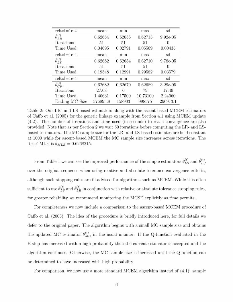
Table 2: Our LR- and LS-based estimators along with the ascent-based MCEM estimatorsof Caffo et al. (2005) for the genetic linkage example from Section 4.1 using MCEM update(4.2). The number of iterations and time used (in seconds) to reach convergence are alsoprovided. Note that as per Section 2 we wait 50 iterations before computing the LR- and LS-based estimators. The MC sample size for the LR- and LS-based estimates are held constantat 1000 while for ascent-based MCEM the MC sample size increases across iterations. The‘true’ MLE is θMLE = 0.6268215.

From Table 1 we can see the improved performance of the simple estimators θ(t)LS and θ

(t)LR

over the original sequence when using relative and absolute tolerance convergence criteria,

although such stopping rules are ill-advised for algorithms such as MCEM. While it is often

sufficient to use θ(t)LS and θ

(t)LR in conjunction with relative or absolute tolerance stopping rules,

for greater reliability we recommend monitoring the MCSE explicitly as time permits.

For completeness we now include a comparison to the ascent-based MCEM procedure of

Caffo et al. (2005). The idea of the procedure is briefly introduced here, for full details we

defer to the original paper. The algorithm begins with a small MC sample size and obtains

the updated MC estimator θ(t)MC in the usual manner. If the Q-function evaluated in the

E-step has increased with a high probability then the current estimator is accepted and the

algorithm continues. Otherwise, the MC sample size is increased until the Q-function can

be determined to have increased with high probability.

For comparison, we now use a more standard MCEM algorithm instead of (4.1): sample

21

U1, U2, · · · , UN ∼ i.i.d Binomial

(y1,

θ(t)MC

2+θ(t)MC

)and let U = 1

N

∑Ni=1 Ui, then set

θ(t+1)MC =

U + y4U + y2 + y3 + y4

. (4.2)

Here we start the ascent-based MCEM procedure with a MC sample size of 1 while the MC

sample size for our LR- and LS-based procedures is kept constant at 1000. The same algo-

rithms are run 100 times independently with a relative tolerance of 10−4 as the convergence

criteria. The LR- and LS-based estimators are first computed after 50 iterations as discussed

in Section 2. Denote the final ascent-based MCEM estimates by θCJJ . Table 2 shows results

for all estimators. All estimators converge to values close to the true MLE, with the ascent-

based MCEM algorithm having slightly improved precision (SD of 0.000033 vs. 0.000099

and 0.000098) at the expense of greater computation time. The mean computation time for

the ascent-based MCEM algorithm is approximately 7 and 30 times greater than the LS-

and LR-based algorithms respectively. This greater computational time is attributable to

the increased MC sample size, with a mean final MC sample size of 576, 895.

We note that, for finite N , the update in (4.2) contains a small bias, thus falling under

the scope of Section 2.4. The use of the same Ui’s in the numerator and denominator induces

a bias on the order of 10−4 for N = 1 when θ(t) is close to the MLE. For N = 1000 the bias

in the one-step update reduces to approximately 8× 10−7. As per Section 2.4, both the LR-

and LS-based estimators will be theoretically biased in this setting, although as seen from

Table 2, the bias for the LS-based estimator is negligible. This suggests, therefore, that the

bias for the LR-based estimator (≈ 2 × 10−5) is a result of the true update operator not

being linear, rather than ε(t)MC in the stochastic update having non-zero expectation.

22

4.2 Example II: Transformation Model for Survival Data with

Gamma Frailty

Secondly, we consider a real data example with a more complicated model setup. A com-

parison with the ascent-based MCEM procedure of Caffo et al. (2005) is again provided.

Clustered survival data arise when the subjects under study are sampled from clusters.

In this section we analyze the litter-matched rats dataset first presented in Mantel et al.

(1977). Three rats from each of 50 litters, one of which received a potential tumorigenic

treatment, are followed for tumor incidence. The time to tumor development is subject to

right-censoring. The proportional hazards frailty model is generally applied to account for

the intra-cluster dependence as well as the censoring. Viewing the frailty as missing data,

the EM algorithm can be implemented for parameter estimation. Since the proportional

hazards assumption is often violated in practice, Zeng and Lin (2007) proposed a broad class

of transformation models to address this. The transformation model is briefly described

below, full details are in Zeng and Lin (2007).

Consider the situation whenM independent clusters are sampled and there are ni subjects

within the ith cluster. The goal is to capture the relationship between the possibly right-

censored survival time Tij and covariates Xij. The right-censoring indicator is denoted by

δij. A shared-frailty ω is introduced to explain the correlation among subjects from the same

cluster and the model can be written as

Λ(u|ωi,Xij) = G(ωi exp(βTXij)Λ0(u)

).

G(·) is a known strictly increasing and continuous differentiable function and Λ0(·) is an

unknown baseline cumulative hazard function. Here, the frailty ωi’s are assumed to be

gamma distributed with mean 1 and variance ν. Let θ = (β, ν,Λ0) where (β, ν) are of

interest and Λ0(·) is considered an infinite dimensional nuisance parameter. Unfortunately,

the conditional expectation involved in the Q function in the E-step cannot be evaluated

23

explicitly and therefore MC integration is needed for the EM algorithm.

For the litter-matched rats data, a binary covariate Xij indicates whether the rat received

the potential tumorigenic treatment. We choose G(x) = log(1 + x) (corresponding to the

proportional odds model) which yields:

Λ(u|ωi, Xij) = log (1 + ωi exp(Xij)u) .

The MCEM algorithm with a MC sample size of 1000 was run to provide three estimators:

θ(t)MC , θ

(t)LS and θ

(t)LR. For illustrative purposes, a relative tolerance of 10−5 was used as the

convergence criteria. We performed 500 independent replications of the algorithm. The

results are summarized in Table 3. The ‘true’ MLE was obtained by running the algorithms

with a large MC sample size for 100,000 iterations (βMLE = 1.02251, νMLE = 0.87502).

For comparison, the ascent-based MCEM procedure was also applied. We started with

a MC sample size of 10 and again performed 500 independent replications of the procedure.

Note that a relative tolerance of 10−3 was used instead of 10−5 because the MC sample size

grew so rapidly that it become computationally infeasible. The estimators are denoted by

βCJJ and νCJJ in Table 3 and the ending MC sample sizes are also reported.

From the results in Table 3 we observe that both the LR- and LS-based estimates converge

within a reasonable number of iterations even under a stringent convergence criteria (a

relative tolerance of 10−5). Moreover, the LR- and LS-based estimates are considerably

more stable than the estimates obtained using ascent-based MCEM, especially for ν. In

terms of computation time, although ascent-based MCEM sometimes converges very rapidly

(the minimum time used is 0.089s), it is, on average, slower than our procedures (mean

time of 92 seconds compared to 22 seconds (LR) and 42 seconds (LS)). There are two

primary reasons why ascent-based MCEM may not be as computationally efficient: (i) the

MC sample size became too large as shown by the ‘Ending MC Size’ in Table 3; (ii) it

inherently involves an additional loop so that the estimates are not accepted until the Q

24

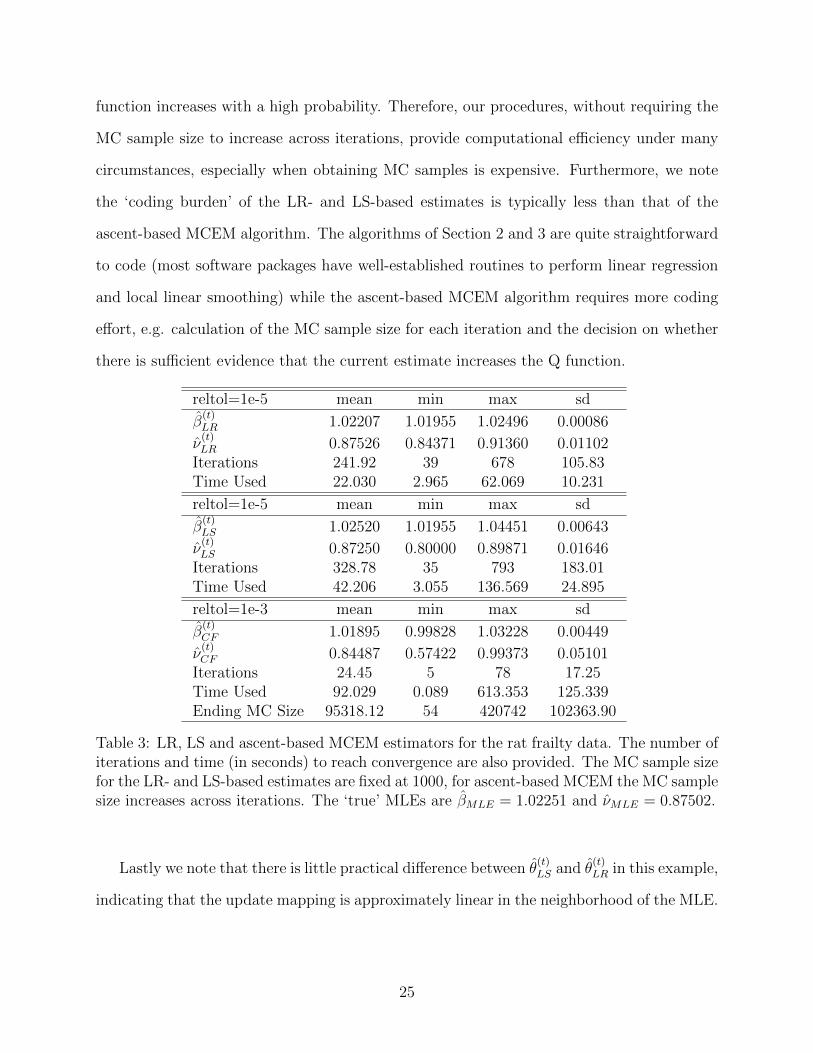
function increases with a high probability. Therefore, our procedures, without requiring the

MC sample size to increase across iterations, provide computational efficiency under many

circumstances, especially when obtaining MC samples is expensive. Furthermore, we note

the ‘coding burden’ of the LR- and LS-based estimates is typically less than that of the

ascent-based MCEM algorithm. The algorithms of Section 2 and 3 are quite straightforward

to code (most software packages have well-established routines to perform linear regression

and local linear smoothing) while the ascent-based MCEM algorithm requires more coding

effort, e.g. calculation of the MC sample size for each iteration and the decision on whether

there is sufficient evidence that the current estimate increases the Q function.

reltol=1e-5 mean min max sd

β(t)LR 1.02207 1.01955 1.02496 0.00086

ν(t)LR 0.87526 0.84371 0.91360 0.01102

Iterations 241.92 39 678 105.83Time Used 22.030 2.965 62.069 10.231

reltol=1e-5 mean min max sd

β(t)LS 1.02520 1.01955 1.04451 0.00643

ν(t)LS 0.87250 0.80000 0.89871 0.01646

Iterations 328.78 35 793 183.01Time Used 42.206 3.055 136.569 24.895

reltol=1e-3 mean min max sd

β(t)CF 1.01895 0.99828 1.03228 0.00449

ν(t)CF 0.84487 0.57422 0.99373 0.05101

Iterations 24.45 5 78 17.25Time Used 92.029 0.089 613.353 125.339Ending MC Size 95318.12 54 420742 102363.90

Table 3: LR, LS and ascent-based MCEM estimators for the rat frailty data. The number ofiterations and time (in seconds) to reach convergence are also provided. The MC sample sizefor the LR- and LS-based estimates are fixed at 1000, for ascent-based MCEM the MC samplesize increases across iterations. The ‘true’ MLEs are βMLE = 1.02251 and νMLE = 0.87502.

Lastly we note that there is little practical difference between θ(t)LS and θ

(t)LR in this example,

indicating that the update mapping is approximately linear in the neighborhood of the MLE.

25

5 Conclusions and Extensions

We have presented a new framework for both estimation and convergence monitoring for

stochastic optimization algorithms such as MCEM. The estimation procedure is simple and

fast to compute, and can provide large gains over standard estimates by reducing MC-induced

variance. Using the MCSE of the estimates to monitor convergence, as discussed in Section 3

provides a reliable, but sometimes computationally expensive, way to monitor convergence.

While there are more sophisticated procedures that can be used to obtain reliable estimates,

our approach can be viewed as a simple alternative to procedures such as those proposed

by Caffo et al. (2005) that requires very minimal user effort to produce improved estimates.

We note that in all discussions, the MCSE of θ is specifically the standard deviation

of θ that is attributable to MC variability, and is fundamentally different from SE(θ), the

uncertainty in the parameter estimate attributable to the data/model. While beyond the

scope of this paper, methods to compute SE(θ) are typically also needed in conjunction with

the methodology for point estimation provided here. Specifically, there has been much work

on standard error estimation using EM and MCEM, which could potentially be combined

with the methodology presented here to simultaneously provide both the MCSE and SE(θ).

For the multivariate problem in section 4.2 we have presented only an element-wise appli-

cation of our estimates. In principle, the correlation across parameters can be accounted for

by estimating the stationary point for all elements of θ simultaneously. In practice, however,

the number of iterations required to reliably estimate the covariance matrix in multivariate

settings is typically large enough for the componentwise approach to be preferred.

In estimating the MCSE of the estimate, analytic approximations can also potentially

allow users to avoid the bootstrap procedure of Section 3. For example, the MCSE of θ(t)LR

can be approximated without using the bootstrap procedure by utilizing knowledge of the

SE of the linear regression-based estimates. These extensions have the potential to speed

up convergence monitoring to accompany the improved estimation procedures presented in

Section 2.

26

Acknowledgments

Research by Jane-Ling Wang was supported by NSF grant DMS-0906813 and NIH grant

1R01-AG025218-01 and 1R56AG043995-01. The authors would also like to thank the editor

and two reviewers for helpful comments that helped to improve an earlier version of the

manuscript.

References

Booth, J. G. and Hobert, J. P. (1999), “Maximizing generalized linear mixed model likeli-

hoods with an automated Monte Carlo EM algorithm,” Journal of the Royal Statistical

Society, Series B, 265–285.

Caffo, B. S., Jank, W., and Jones, G. L. (2005), “Ascent-based Monte Carlo EM,” Journal

of the Royal Statistical Society, Series B, 67, 235–251.

Chan, K. S. and Ledolter, J. (1995), “Monte Carlo EM estimation for time series involving

counts,” Journal of the American Statistical Association, 90, 242–252.

Cleveland, W. S. (1979), “Robust locally weighted regression and smoothing scatterplots,”

Journal of the American statistical association, 74, 829–836.

Dempster, A. P., Laird, N. M., and Rubin, D. B. (1977), “Maximum Likelihood from In-

complete Data via the EM Algorithm,” Journal of the Royal Statistical Society, Series B

(Methodological), 39, 1–38.

Epanechnikov, V. A. (1969), “Non-parametric estimation of a multivariate probability den-

sity,” Theory of Probability & Its Applications, 14, 153–158.

Fort, G. and Moulines, E. (2003), “Convergence of the Monte Carlo expectation maximiza-

tion for curved exponential families,” The Annals of Statistics, 31, 1220–1259.

27

Gasser, T., Muller, H. G., and Mammitzsch, V. (1985), “Kernels for nonparametric curve

estimation,” Journal of the Royal Statistical Society, Series B (Methodological), 47, 238–

252.

Hardle, W. and Tsybakov, A. (1997), “Local polynomial estimators of the volatility function

in nonparametric autoregression,” Journal of Econometrics, 81, 223–242.

Jones, G. L. (2004), “On the Markov chain central limit theorem,” Probability surveys, 1,

299–320.

Levine, R. A. and Casella, G. (2001), “Implementations of the Monte Carlo EM algorithm,”

Journal of Computational and Graphical Statistics, 10, 422–439.

Mantel, N., Bohidar, N. R., and Ciminera, J. L. (1977), “Mantel-Haenszel analyses of litter-

matched time-to-response data, with modifications for recovery of interlitter information,”

Cancer Research, 37, 3863–3868.

Masry, E. (1996), “Multivariate local polynomial regression for time series: uniform strong

consistency and rates,” Journal of Time Series Analysis, 17, 571–599.

McCulloch, C. E. (1994), “Maximum likelihood variance components estimation for binary

data,” Journal of the American Statistical Association, 89, 330–335.

— (1997), “Maximum likelood algorithms for generalized linear mixed models,” Journal of

the American Statistical Association, 92, 162–170.

Neath, R. C. (2012), “On convergence properties of the Monte Carlo EM algorithm,” IMS

Collections.

Nummelin, E. and Tuominen, P. (1982), “Geometric ergodicity of Harris-recurrent Markov

chains with application to renewal theory,” Stochastic Processes and their Applications,

12, 187–202.

28

Shi, J. Q. and Copas, J. (2002), “Publication bias and meta-analysis for 2× 2 tables: an av-

erage Markov chain Monte Carlo EM algorithm,” Journal of the Royal Statistical Society,

Series B (Statistical Methodology), 64, 221–236.

Stone, C. J. (1977), “Consistent nonparametric regression,” The Annals of Statistics, 5,

595–620.

Wei, G. C. G. and Tanner, M. A. (1990), “A Monte Carlo implementation of the EM al-

gorithm and the poor man’s data augmentation algorithms,” Journal of the American

Statistical Association, 85, 699–704.

Zeng, D. and Lin, D. Y. (2007), “Maximum likelihood estimation in semiparametric re-

gression models with censored data,” Journal of the Royal Statistical Society, Series B

(Statistical Methodology), 69, 507–564.

Appendix

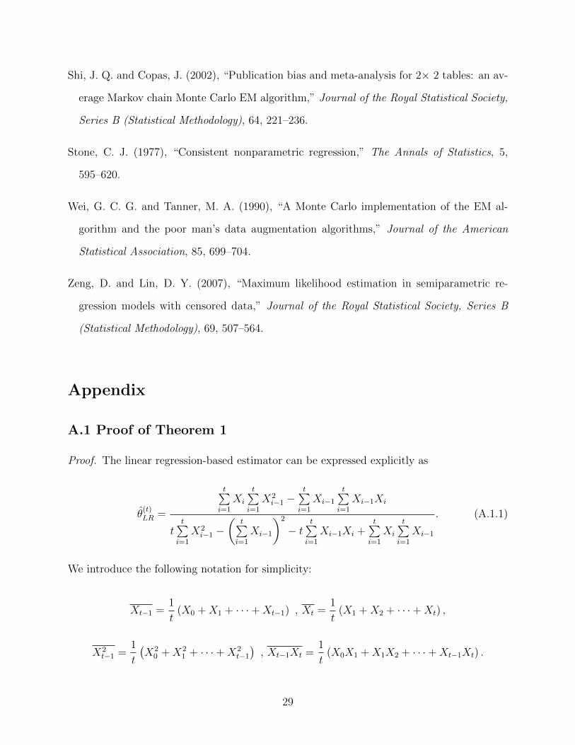
A.1 Proof of Theorem 1

Proof. The linear regression-based estimator can be expressed explicitly as

θ(t)LR =

t∑i=1

Xi

t∑i=1

X2i−1 −

t∑i=1

Xi−1t∑i=1

Xi−1Xi

tt∑i=1

X2i−1 −

(t∑i=1

Xi−1

)2

− tt∑i=1

Xi−1Xi +t∑i=1

Xi

t∑i=1

Xi−1

. (A.1.1)

We introduce the following notation for simplicity:

Xt−1 =1

t(X0 +X1 + · · ·+Xt−1) , Xt =

1

t(X1 +X2 + · · ·+Xt) ,

X2t−1 =

1

t

(X2

0 +X21 + · · ·+X2

t−1)

, Xt−1Xt =1

t(X0X1 +X1X2 + · · ·+Xt−1Xt) .

29

After some calculation, the linear regression-based estimator in (A.1.1) can be rewritten as

θ(t)LR =

Xt−1

(X2t−1 −Xt−1Xt

)+X2

t−1(Xt −Xt−1

)(X2t−1 −Xt−1Xt

)+Xt−1

(Xt −Xt−1

) . (A.1.2)

Since

Xt −Xt−1 =1

t(Xt −X0)

a.s.−−−→t→∞

0,

from (A.1.2) we find that θ(t)LR is asymptotically equivalent to Xt−1 and by the ergodic theorem

θ(t)LR

a.s.−−−→t→∞

Eπ(X). (A.1.3)

Under (2.2) and the assumptions in Section 2.1, the stationary density π(·) satisfies

π(y) =

∫π(x)

s(x)φ

(y −m(x)

s(x)

)dx,

where φ(·) is the density of ε(t)MC . Then

Eπ(X) =∫yπ(y)dy =

∫y

(∫π(x)

s(x)φ

(y −m(x)

s(x)

)dx

)dy

=

∫π(x)

s(x)

(∫yφ

(y −m(x)

s(x)

)dy

)dx =

∫π(x)m(x)dx.

Therefore by Taylor expansion and the fact that θ∗ = m(θ∗),

Eπ(X)− θ∗ =∫π(x) [m(x)−m(θ∗)] dx

=

∫π(x)

[m′(θ∗)(x− θ∗) +

∞∑k=2

m(k)(θ∗)

k!(x− θ∗)k

]dx

= m′(θ∗) [Eπ(X)− θ∗] +∞∑k=2

m(k)(θ∗)

k!Eφ(X − θ∗)k.

(A.1.4)

Conclusion (2.5) is obtained by combining (A.1.3) with (A.1.4). For (2.6), it is a direct result

of Theorem 4 from Jones (2004).

30

A.2 Proof of Theorem 2

Proof. We prove Theorem 2 using the results of Theorem 6 in Masry (1996). For complete-

ness, we state the theorem below using the notations in this paper.

Theorem 3. (Theorem 6 in Masry (1996)) Under C1-C7 the local linear smoother mLSt (x)

satisfies that for any compact set X ∈ R

supx∈X|mLS

t (x)−m(x)| a.s.−−→ 0, (A.2.1)

supx∈X|mLS

t (x)−m(x)| = O

{(log t

t

) 25

}a.s. (A.2.2)

First, we show the existence of quasi-stationary points of mLSt (x) in (a, b). From (A.2.2), we

have

|mLSt (θ∗)− θ∗| = |mLS

t (θ∗)−m(θ∗)| = O

{(log t

t

) 25

}.

Therefore, at least θ∗ is a quasi-stationary point of mLSt (x) in (a, b). Let θ

(t)LS ∈ (a, b) be an

arbitrary quasi-stationary point of mLSt (x), consider

θ(t)LS − θ∗ = mLS

t (θ(t)LS)−m(θ∗) +O

{(log tt

) 25

}=

[mLSt (θ

(t)LS)−m(θ

(t)LS)]

+[m(θ

(t)LS)−m(θ∗)

]+O

{(log tt

) 25

}a.s.

(A.2.3)

By Taylor expansion, the second term on the second line of (A.2.3) satisfies (for some θ

between θ(t)LS and θ∗)

m(θ(t)LS)−m(θ∗) = m′(θ)(θ

(t)LS − θ

∗).

Hence

θ(t)LS − θ

∗ =mLSt (θ

(t)LS)−m(θ

(t)LS)

1−m′(θ)+O

{(log t

t

) 25

}a.s. (A.2.4)

By (A.2.1), the numerator in (A.2.4) converges to 0 almost surely and θ(t)LS

a.s.−−→ θ∗ follows

31

immediately. Similarly, (2.9) follows from (A.2.2). This completes the proof.

32