Implementation of a user-defined time integration in FEAP:...
22
Report No. Structural Engineering UCB/SEMM-2010/07 Mechanics and Materials Implementation of a user-defined time integration in FEAP: Wilson-Θ By Karl Steeger Mentor: Sanjay Govindjee July 2010 Department of Civil and Environmental Engineering University of California, Berkeley
Transcript of Implementation of a user-defined time integration in FEAP:...
Report No. Structural EngineeringUCB/SEMM-2010/07 Mechanics and Materials
Implementation of a user-definedtime integration in FEAP:Wilson-Θ
By Karl Steeger
Mentor: Sanjay Govindjee
July 2010 Department of Civil and Environmental EngineeringUniversity of California, Berkeley
K. Steeger 1
Contents
1 The Wilson-Θ Method 4
1.1 Derivation of the Wilson-Θ Method . . . . . . . . . . . . . . . . . . . . . . 4
1.2 Stability of the Wilson-Θ Method . . . . . . . . . . . . . . . . . . . . . . . 5
2 Abstract - How to program 5
2.1 Given displacements (d-form) . . . . . . . . . . . . . . . . . . . . . . . . . 5
2.2 Implemetation steps in FEAP . . . . . . . . . . . . . . . . . . . . . . . . . 7
2.2.1 udynam.f . . . . . . . . . . . . . . . . . . . . . . . . . . . . . . . . 8
2.2.2 dparam.f/uparam.f . . . . . . . . . . . . . . . . . . . . . . . . . . . 12
2.2.3 dsetci.f/usetci.f . . . . . . . . . . . . . . . . . . . . . . . . . . . . . 14
2.2.4 Inputfile . . . . . . . . . . . . . . . . . . . . . . . . . . . . . . . . . 16
3 Numerical Example 16
3.1 Description of the problem . . . . . . . . . . . . . . . . . . . . . . . . . . . 16
3.2 Evaluation . . . . . . . . . . . . . . . . . . . . . . . . . . . . . . . . . . . . 19
Finite Elements for Elastodynamics 2
List of Figures
1 The Wilson-Θ Method. . . . . . . . . . . . . . . . . . . . . . . . . . . . . . 4
2 Running schedule . . . . . . . . . . . . . . . . . . . . . . . . . . . . . . . . 7
3 Main parts of udynam.f for isw = 1. . . . . . . . . . . . . . . . . . . . . . 10
4 Main parts of udynam.f for isw = 2. . . . . . . . . . . . . . . . . . . . . . 11
5 Main parts of udynam.f for isw = 3. . . . . . . . . . . . . . . . . . . . . . 12
6 Main parts of uparam.f. . . . . . . . . . . . . . . . . . . . . . . . . . . . . 15
7 Main parts of usetci.f. . . . . . . . . . . . . . . . . . . . . . . . . . . . . . 16
8 Setup Cook’s membrane. . . . . . . . . . . . . . . . . . . . . . . . . . . . . 17
9 Inputfile for Cook’s Membrane. . . . . . . . . . . . . . . . . . . . . . . . . 18
10 Procedure to run inputfile. . . . . . . . . . . . . . . . . . . . . . . . . . . . 19
11 Cook’s Membrane u2-displacement upper right node. . . . . . . . . . . . . 20
K. Steeger 3
List of Tables
1 Different cases for isw in udynam.f. . . . . . . . . . . . . . . . . . . . . . . 8
2 isw independent variables in udynam.f. . . . . . . . . . . . . . . . . . . . . 8
3 Passed variables for isw = 1 in udynam.f. . . . . . . . . . . . . . . . . . . . 9
4 Passed variables for isw = 2 in udynam.f. . . . . . . . . . . . . . . . . . . . 11
5 Passed variables in dparam.f. . . . . . . . . . . . . . . . . . . . . . . . . . 12
6 Passed variables in uparam.f. . . . . . . . . . . . . . . . . . . . . . . . . . 13
7 Setup of variables in uparam.f. . . . . . . . . . . . . . . . . . . . . . . . . . 14
8 Parameters cc1, cc2 and cc3. . . . . . . . . . . . . . . . . . . . . . . . . . . 15
9 Residual satisfaction. . . . . . . . . . . . . . . . . . . . . . . . . . . . . . . 19
Finite Elements for Elastodynamics 4
1 The Wilson-Θ Method
The FEAP internal structure provides different time integration schemes like Newmark,HHT, etc.. Additionally it is possible to add a user defined one.
A possible scheme for time integration is the Wilson-Θ method. The Wilson-Θ Method isa linear multistep method for second order equations, see Wilson et al. [1973] and Hughes[1987].
1.1 Derivation of the Wilson-Θ Method
The time-dependent system of equations which has to be solved is written as
Md + Cd + Kd = F , (1)
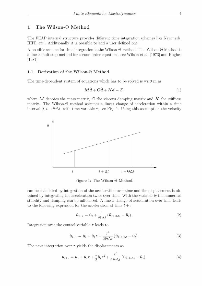
where M denotes the mass matrix, C the viscous damping matrix and K the stiffnessmatrix. The Wilson-Θ method assumes a linear change of acceleration within a timeinterval [t, t + Θ∆t] with time variable τ , see Fig. 1. Using this assumption the velocity
t + ∆t t + Θ∆t
u
t
τ
Figure 1: The Wilson-Θ Method.
can be calculated by integration of the acceleration over time and the displacement is ob-tained by integrating the acceleration twice over time. With the variable Θ the numericalstability and damping can be influenced. A linear change of acceleration over time leadsto the following expression for the acceleration at time t + τ
ut+τ = ut +τ
Θ∆t(ut+Θ∆t − ut) . (2)
Integration over the control variable τ leads to
ut+τ = ut + utτ +τ 2
2Θ∆t(ut+Θ∆t − ut) . (3)
The next integration over τ yields the displacements as
ut+τ = ut + utτ +1
2utτ
2 +τ 3
6Θ∆t(ut+Θ∆t − ut) . (4)
K. Steeger 5
Now we replace the control variable τ with the expression Θ∆t in the equations for velocityand displacements and simplify. We obtain
ut+Θ∆t = ut +Θ∆t
2(ut+Θ∆t + ut)
ut+Θ∆t = ut + Θ∆tut +1
6(Θ∆t)2 (ut+Θ∆t + 2ut) .
(5)
1.2 Stability of the Wilson-Θ Method
The Wilson method is unconditionally stable for Θ ≥ 1.37. Further information concern-ing stability and accuracy can be found in Hughes [1987], Gladwell and Thomas [1980]and Wilson et al. [1973].
2 Abstract - How to program
To program this, we could differentiate between three different cases, depending on whichvariable is solved by the sytem of equations and which variables has to be calculated by thetime integration scheme. Here we just consider the formulation where the displacementis the solution variable. For our calculation we need the values of the displcement, thevelocity and the acceleration at different points in time.
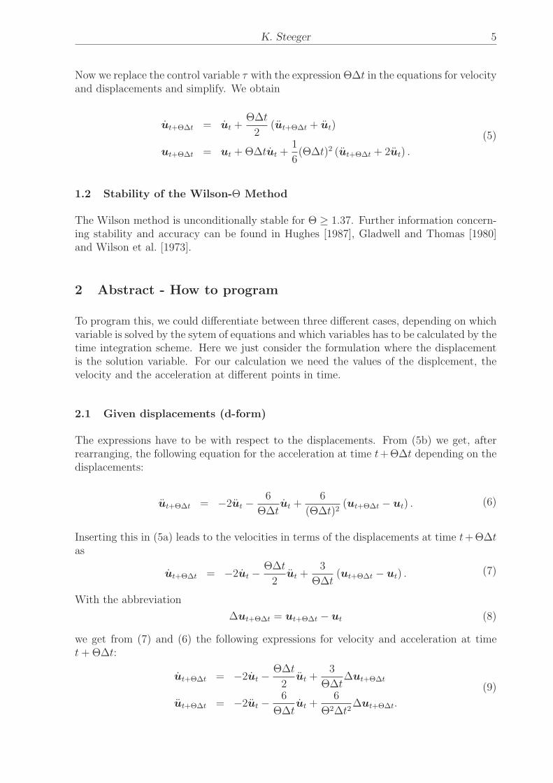
2.1 Given displacements (d-form)
The expressions have to be with respect to the displacements. From (5b) we get, afterrearranging, the following equation for the acceleration at time t+Θ∆t depending on thedisplacements:
ut+Θ∆t = −2ut −6
Θ∆tut +
6
(Θ∆t)2(ut+Θ∆t − ut) . (6)
Inserting this in (5a) leads to the velocities in terms of the displacements at time t+Θ∆t
as
ut+Θ∆t = −2ut −Θ∆t
2ut +
3
Θ∆t(ut+Θ∆t − ut) . (7)
With the abbreviation
∆ut+Θ∆t = ut+Θ∆t − ut (8)
we get from (7) and (6) the following expressions for velocity and acceleration at timet + Θ∆t:
ut+Θ∆t = −2ut −Θ∆t
2ut +
3
Θ∆t∆ut+Θ∆t
ut+Θ∆t = −2ut −6
Θ∆tut +
6
Θ2∆t2∆ut+Θ∆t.
(9)
Finite Elements for Elastodynamics 6
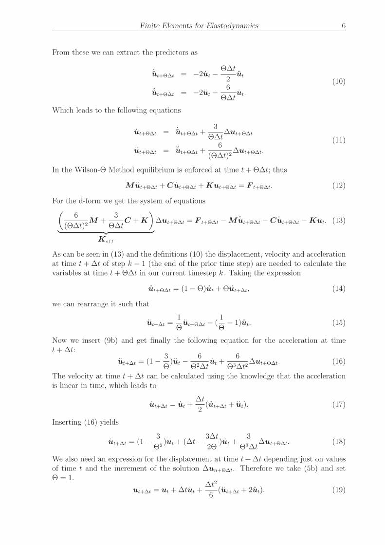
From these we can extract the predictors as
˙ut+Θ∆t = −2ut −Θ∆t
2ut
¨ut+Θ∆t = −2ut −6
Θ∆tut.
(10)
Which leads to the following equations
ut+Θ∆t = ˙ut+Θ∆t +3
Θ∆t∆ut+Θ∆t
ut+Θ∆t = ¨ut+Θ∆t +6
(Θ∆t)2∆ut+Θ∆t.
(11)
In the Wilson-Θ Method equilibrium is enforced at time t + Θ∆t; thus
Mut+Θ∆t + Cut+Θ∆t + Kut+Θ∆t = F t+Θ∆t. (12)
For the d-form we get the system of equations(
6
(Θ∆t)2M +
3
Θ∆tC + K
)
︸ ︷︷ ︸
Keff
∆ut+Θ∆t = F t+Θ∆t − M ¨ut+Θ∆t − C ˙ut+Θ∆t − Kut. (13)
As can be seen in (13) and the definitions (10) the displacement, velocity and accelerationat time t + ∆t of step k − 1 (the end of the prior time step) are needed to calculate thevariables at time t + Θ∆t in our current timestep k. Taking the expression
ut+Θ∆t = (1 − Θ)ut + Θut+∆t, (14)
we can rearrange it such that
ut+∆t =1
Θut+Θ∆t − (
1
Θ− 1)ut. (15)
Now we insert (9b) and get finally the following equation for the acceleration at timet + ∆t:
ut+∆t = (1 −3
Θ)ut −
6
Θ2∆tut +
6
Θ3∆t2∆ut+Θ∆t. (16)
The velocity at time t + ∆t can be calculated using the knowledge that the accelerationis linear in time, which leads to
ut+∆t = ut +∆t
2(ut+∆t + ut). (17)
Inserting (16) yields
ut+∆t = (1 −3
Θ2)ut + (∆t −
3∆t
2Θ)ut +
3
Θ3∆t∆ut+Θ∆t. (18)
We also need an expression for the displacement at time t + ∆t depending just on valuesof time t and the increment of the solution ∆un+Θ∆t. Therefore we take (5b) and setΘ = 1.
ut+∆t = ut + ∆tut +∆t2
6(ut+∆t + 2ut). (19)
K. Steeger 7
Now we insert (16) and finally get
ut+∆t = ut + (1 −1
Θ2)∆tut + (1 −
1
Θ)∆t2
2ut +
1
Θ3∆ut+Θ∆t. (20)
From that we can extract a predictor
ut+∆t = ut + (1 −1
Θ2)∆tut + (1 −
1
Θ)∆t2
2ut (21)
and get the final expression
ut+∆t = ut+∆t +1
Θ3∆ut+Θ∆t (22)
respectively
∆ut+∆t = ut+∆t − ut = −ut + ut+∆t +1
Θ3∆ut+Θ∆t. (23)
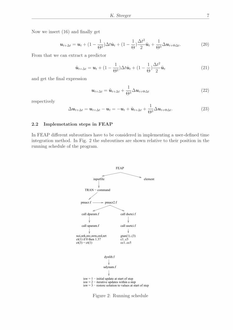
2.2 Implemetation steps in FEAP
In FEAP different subroutines have to be considered in implementing a user-defined timeintegration method. In Fig. 2 the subroutines are shown relative to their position in therunning schedule of the program.
noi,nrk,nrc,nrm,ord,nrtct(1) if 0 then 1.37ct(3) = ct(1)
isw = 3 − restore solution to values at start of stepisw = 2 − iterative updates within a stepisw = 1 − initial update at start of step
gtan(1)..(3)c1..c5cc1..cc5
FEAP
TRAN − command
elementinputfile
pmacr2.fpmacr.f
call dsetci.f
call usetci.f
dynlib.f
udynam.f
call uparam.f
call dparam.f
Figure 2: Running schedule
Finite Elements for Elastodynamics 8
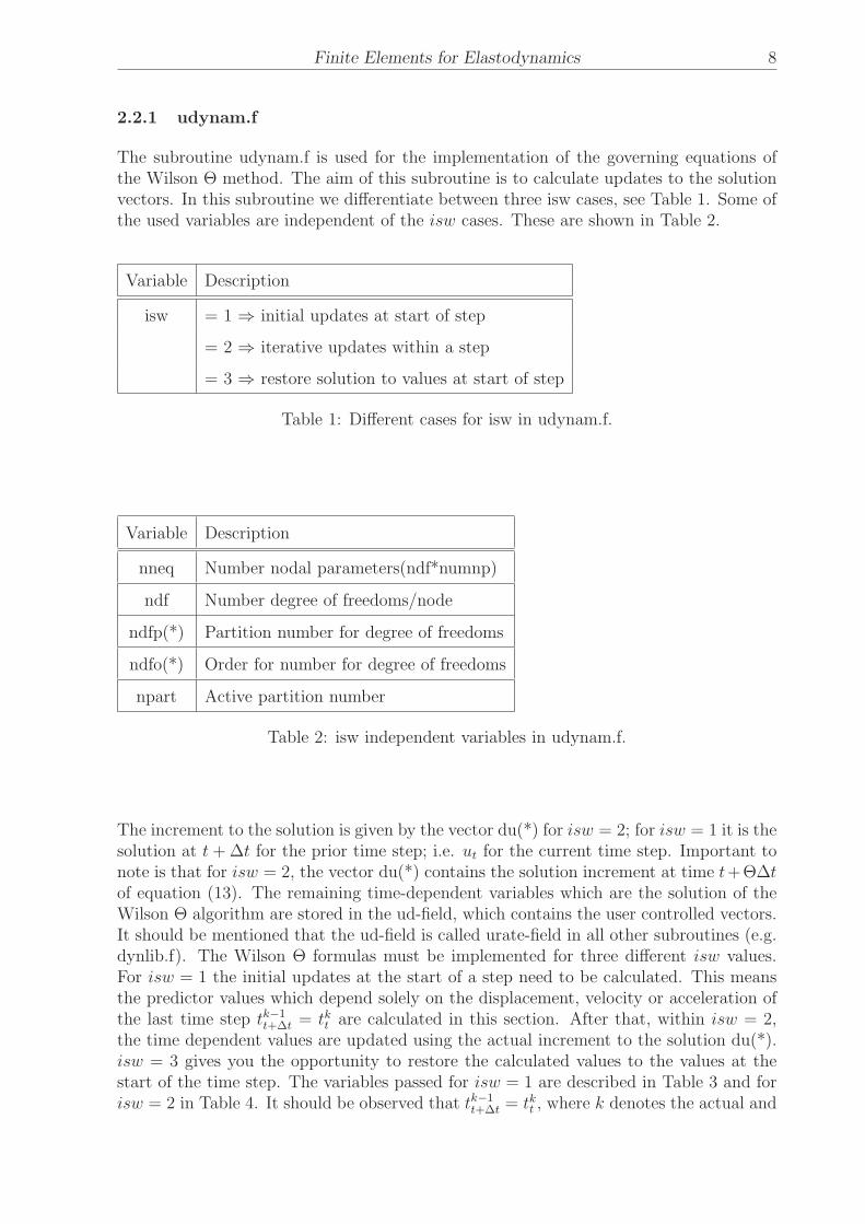
2.2.1 udynam.f
The subroutine udynam.f is used for the implementation of the governing equations ofthe Wilson Θ method. The aim of this subroutine is to calculate updates to the solutionvectors. In this subroutine we differentiate between three isw cases, see Table 1. Some ofthe used variables are independent of the isw cases. These are shown in Table 2.
Variable Description
isw = 1 ⇒ initial updates at start of step
= 2 ⇒ iterative updates within a step
= 3 ⇒ restore solution to values at start of step
Table 1: Different cases for isw in udynam.f.
Variable Description
nneq Number nodal parameters(ndf*numnp)
ndf Number degree of freedoms/node
ndfp(*) Partition number for degree of freedoms
ndfo(*) Order for number for degree of freedoms
npart Active partition number
Table 2: isw independent variables in udynam.f.
The increment to the solution is given by the vector du(*) for isw = 2; for isw = 1 it is thesolution at t + ∆t for the prior time step; i.e. ut for the current time step. Important tonote is that for isw = 2, the vector du(*) contains the solution increment at time t+Θ∆t
of equation (13). The remaining time-dependent variables which are the solution of theWilson Θ algorithm are stored in the ud-field, which contains the user controlled vectors.It should be mentioned that the ud-field is called urate-field in all other subroutines (e.g.dynlib.f). The Wilson Θ formulas must be implemented for three different isw values.For isw = 1 the initial updates at the start of a step need to be calculated. This meansthe predictor values which depend solely on the displacement, velocity or acceleration ofthe last time step tk−1
t+∆t= tk
tare calculated in this section. After that, within isw = 2,
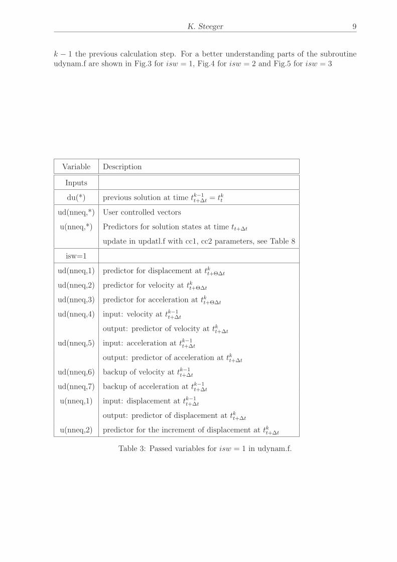
the time dependent values are updated using the actual increment to the solution du(*).isw = 3 gives you the opportunity to restore the calculated values to the values at thestart of the time step. The variables passed for isw = 1 are described in Table 3 and forisw = 2 in Table 4. It should be observed that tk−1
t+∆t= tk
t, where k denotes the actual and
K. Steeger 9
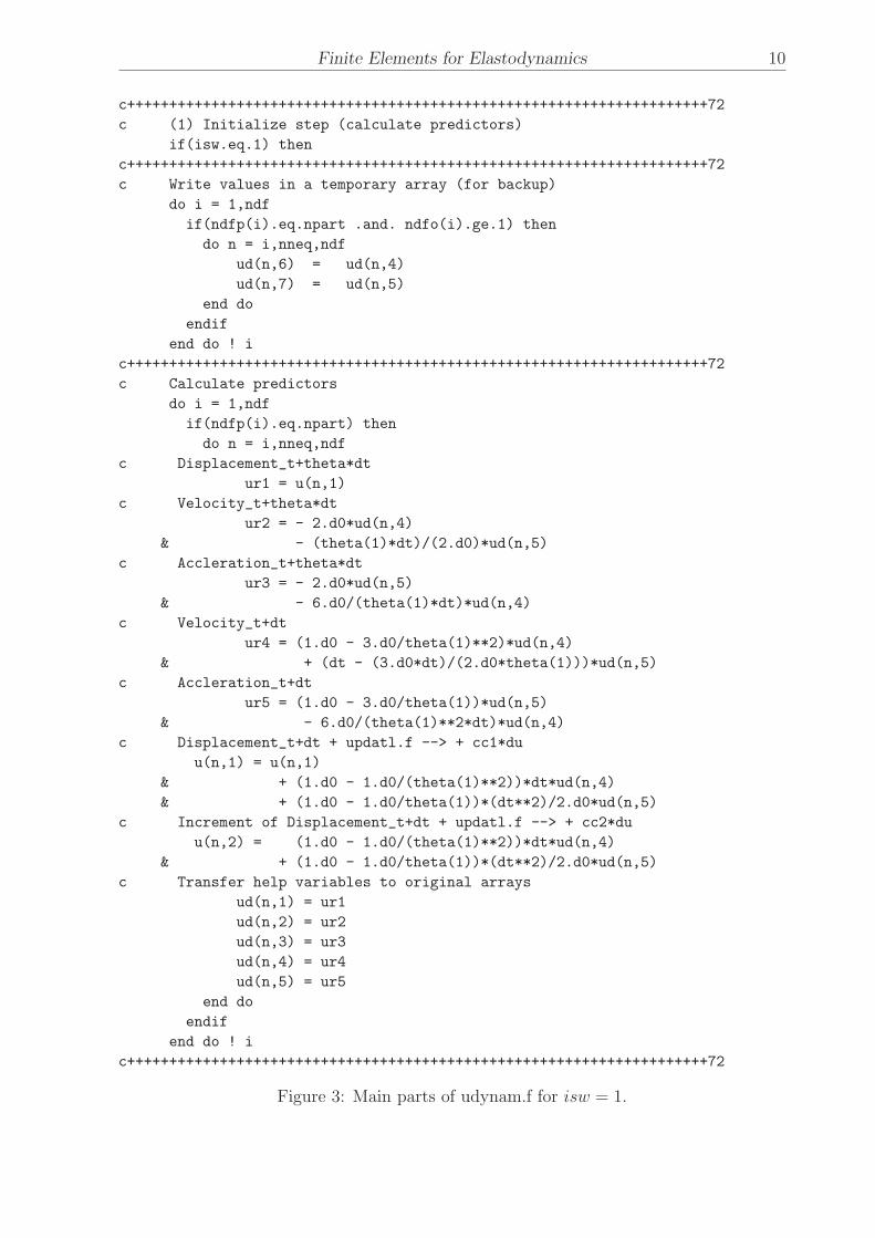
k − 1 the previous calculation step. For a better understanding parts of the subroutineudynam.f are shown in Fig.3 for isw = 1, Fig.4 for isw = 2 and Fig.5 for isw = 3
Variable Description
Inputs
du(*) previous solution at time tk−1
t+∆t= tk
t
ud(nneq,*) User controlled vectors
u(nneq,*) Predictors for solution states at time tt+∆t
update in updatl.f with cc1, cc2 parameters, see Table 8
isw=1
ud(nneq,1) predictor for displacement at tkt+Θ∆t
ud(nneq,2) predictor for velocity at tkt+Θ∆t
ud(nneq,3) predictor for acceleration at tkt+Θ∆t
ud(nneq,4) input: velocity at tk−1
t+∆t
output: predictor of velocity at tkt+∆t
ud(nneq,5) input: acceleration at tk−1
t+∆t
output: predictor of acceleration at tkt+∆t
ud(nneq,6) backup of velocity at tk−1
t+∆t
ud(nneq,7) backup of acceleration at tk−1
t+∆t
u(nneq,1) input: displacement at tk−1
t+∆t
output: predictor of displacement at tkt+∆t
u(nneq,2) predictor for the increment of displacement at tkt+∆t
Table 3: Passed variables for isw = 1 in udynam.f.
Finite Elements for Elastodynamics 10
c+++++++++++++++++++++++++++++++++++++++++++++++++++++++++++++++++++++72
c (1) Initialize step (calculate predictors)
if(isw.eq.1) then
c+++++++++++++++++++++++++++++++++++++++++++++++++++++++++++++++++++++72
c Write values in a temporary array (for backup)
do i = 1,ndf
if(ndfp(i).eq.npart .and. ndfo(i).ge.1) then
do n = i,nneq,ndf
ud(n,6) = ud(n,4)
ud(n,7) = ud(n,5)
end do
endif
end do ! i
c+++++++++++++++++++++++++++++++++++++++++++++++++++++++++++++++++++++72
c Calculate predictors
do i = 1,ndf
if(ndfp(i).eq.npart) then
do n = i,nneq,ndf
c Displacement_t+theta*dt
ur1 = u(n,1)
c Velocity_t+theta*dt
ur2 = - 2.d0*ud(n,4)
& - (theta(1)*dt)/(2.d0)*ud(n,5)
c Accleration_t+theta*dt
ur3 = - 2.d0*ud(n,5)
& - 6.d0/(theta(1)*dt)*ud(n,4)
c Velocity_t+dt
ur4 = (1.d0 - 3.d0/theta(1)**2)*ud(n,4)
& + (dt - (3.d0*dt)/(2.d0*theta(1)))*ud(n,5)
c Accleration_t+dt
ur5 = (1.d0 - 3.d0/theta(1))*ud(n,5)
& - 6.d0/(theta(1)**2*dt)*ud(n,4)
c Displacement_t+dt + updatl.f --> + cc1*du
u(n,1) = u(n,1)
& + (1.d0 - 1.d0/(theta(1)**2))*dt*ud(n,4)
& + (1.d0 - 1.d0/theta(1))*(dt**2)/2.d0*ud(n,5)
c Increment of Displacement_t+dt + updatl.f --> + cc2*du
u(n,2) = (1.d0 - 1.d0/(theta(1)**2))*dt*ud(n,4)
& + (1.d0 - 1.d0/theta(1))*(dt**2)/2.d0*ud(n,5)
c Transfer help variables to original arrays
ud(n,1) = ur1
ud(n,2) = ur2
ud(n,3) = ur3
ud(n,4) = ur4
ud(n,5) = ur5
end do
endif
end do ! i
c+++++++++++++++++++++++++++++++++++++++++++++++++++++++++++++++++++++72
Figure 3: Main parts of udynam.f for isw = 1.
K. Steeger 11
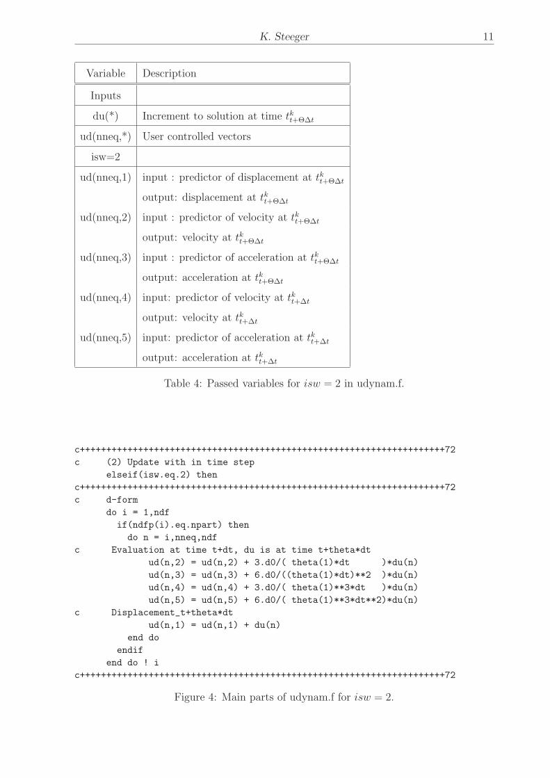
Variable Description
Inputs
du(*) Increment to solution at time tkt+Θ∆t
ud(nneq,*) User controlled vectors
isw=2
ud(nneq,1) input : predictor of displacement at tkt+Θ∆t
output: displacement at tkt+Θ∆t
ud(nneq,2) input : predictor of velocity at tkt+Θ∆t
output: velocity at tkt+Θ∆t
ud(nneq,3) input : predictor of acceleration at tkt+Θ∆t
output: acceleration at tkt+Θ∆t
ud(nneq,4) input: predictor of velocity at tkt+∆t
output: velocity at tkt+∆t
ud(nneq,5) input: predictor of acceleration at tkt+∆t
output: acceleration at tkt+∆t
Table 4: Passed variables for isw = 2 in udynam.f.
c+++++++++++++++++++++++++++++++++++++++++++++++++++++++++++++++++++++72
c (2) Update with in time step
elseif(isw.eq.2) then
c+++++++++++++++++++++++++++++++++++++++++++++++++++++++++++++++++++++72
c d-form
do i = 1,ndf
if(ndfp(i).eq.npart) then
do n = i,nneq,ndf
c Evaluation at time t+dt, du is at time t+theta*dt
ud(n,2) = ud(n,2) + 3.d0/( theta(1)*dt )*du(n)
ud(n,3) = ud(n,3) + 6.d0/((theta(1)*dt)**2 )*du(n)
ud(n,4) = ud(n,4) + 3.d0/( theta(1)**3*dt )*du(n)
ud(n,5) = ud(n,5) + 6.d0/( theta(1)**3*dt**2)*du(n)
c Displacement_t+theta*dt
ud(n,1) = ud(n,1) + du(n)
end do
endif
end do ! i
c+++++++++++++++++++++++++++++++++++++++++++++++++++++++++++++++++++++72
Figure 4: Main parts of udynam.f for isw = 2.
Finite Elements for Elastodynamics 12
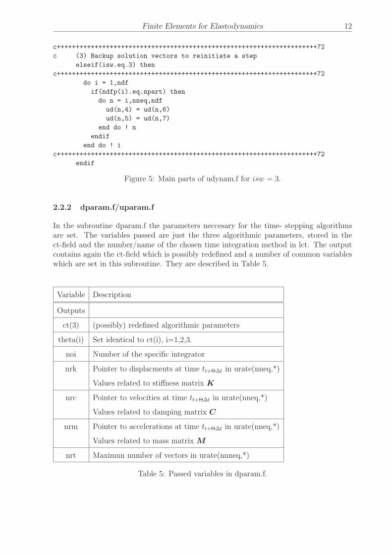
c+++++++++++++++++++++++++++++++++++++++++++++++++++++++++++++++++++++72
c (3) Backup solution vectors to reinitiate a step
elseif(isw.eq.3) then
c+++++++++++++++++++++++++++++++++++++++++++++++++++++++++++++++++++++72
do i = 1,ndf
if(ndfp(i).eq.npart) then
do n = i,nneq,ndf
ud(n,4) = ud(n,6)
ud(n,5) = ud(n,7)
end do ! n
endif
end do ! i
c+++++++++++++++++++++++++++++++++++++++++++++++++++++++++++++++++++++72
endif
Figure 5: Main parts of udynam.f for isw = 3.
2.2.2 dparam.f/uparam.f
In the subroutine dparam.f the parameters neccesary for the time- stepping algorithmsare set. The variables passed are just the three algorithmic parameters, stored in thect-field and the number/name of the chosen time integration method in lct. The outputcontains again the ct-field which is possibly redefined and a number of common variableswhich are set in this subroutine. They are described in Table 5.
Variable Description
Outputs
ct(3) (possibly) redefined algorithmic parameters
theta(i) Set identical to ct(i), i=1,2,3.
noi Number of the specific integrator
nrk Pointer to displacments at time tt+Θ∆t in urate(nneq,*)
Values related to stiffness matrix K
nrc Pointer to velocities at time tt+Θ∆t in urate(nneq,*)
Values related to damping matrix C
nrm Pointer to accelerations at time tt+Θ∆t in urate(nneq,*)
Values related to mass matrix M
nrt Maximun number of vectors in urate(nnneq,*)
Table 5: Passed variables in dparam.f.
K. Steeger 13
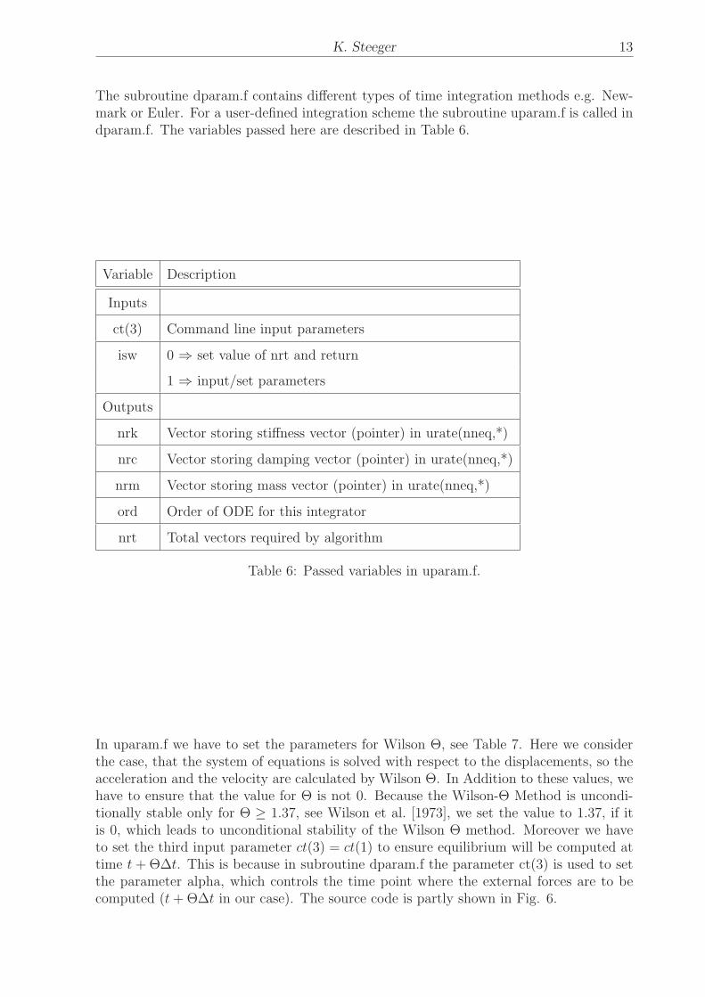
The subroutine dparam.f contains different types of time integration methods e.g. New-mark or Euler. For a user-defined integration scheme the subroutine uparam.f is called indparam.f. The variables passed here are described in Table 6.
Variable Description
Inputs
ct(3) Command line input parameters
isw 0 ⇒ set value of nrt and return
1 ⇒ input/set parameters
Outputs
nrk Vector storing stiffness vector (pointer) in urate(nneq,*)
nrc Vector storing damping vector (pointer) in urate(nneq,*)
nrm Vector storing mass vector (pointer) in urate(nneq,*)
ord Order of ODE for this integrator
nrt Total vectors required by algorithm
Table 6: Passed variables in uparam.f.
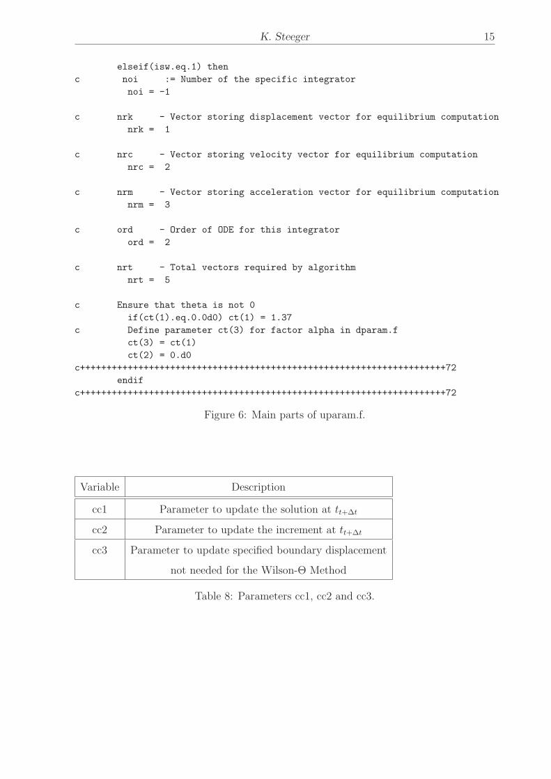
In uparam.f we have to set the parameters for Wilson Θ, see Table 7. Here we considerthe case, that the system of equations is solved with respect to the displacements, so theacceleration and the velocity are calculated by Wilson Θ. In Addition to these values, wehave to ensure that the value for Θ is not 0. Because the Wilson-Θ Method is uncondi-tionally stable only for Θ ≥ 1.37, see Wilson et al. [1973], we set the value to 1.37, if itis 0, which leads to unconditional stability of the Wilson Θ method. Moreover we haveto set the third input parameter ct(3) = ct(1) to ensure equilibrium will be computed attime t + Θ∆t. This is because in subroutine dparam.f the parameter ct(3) is used to setthe parameter alpha, which controls the time point where the external forces are to becomputed (t + Θ∆t in our case). The source code is partly shown in Fig. 6.
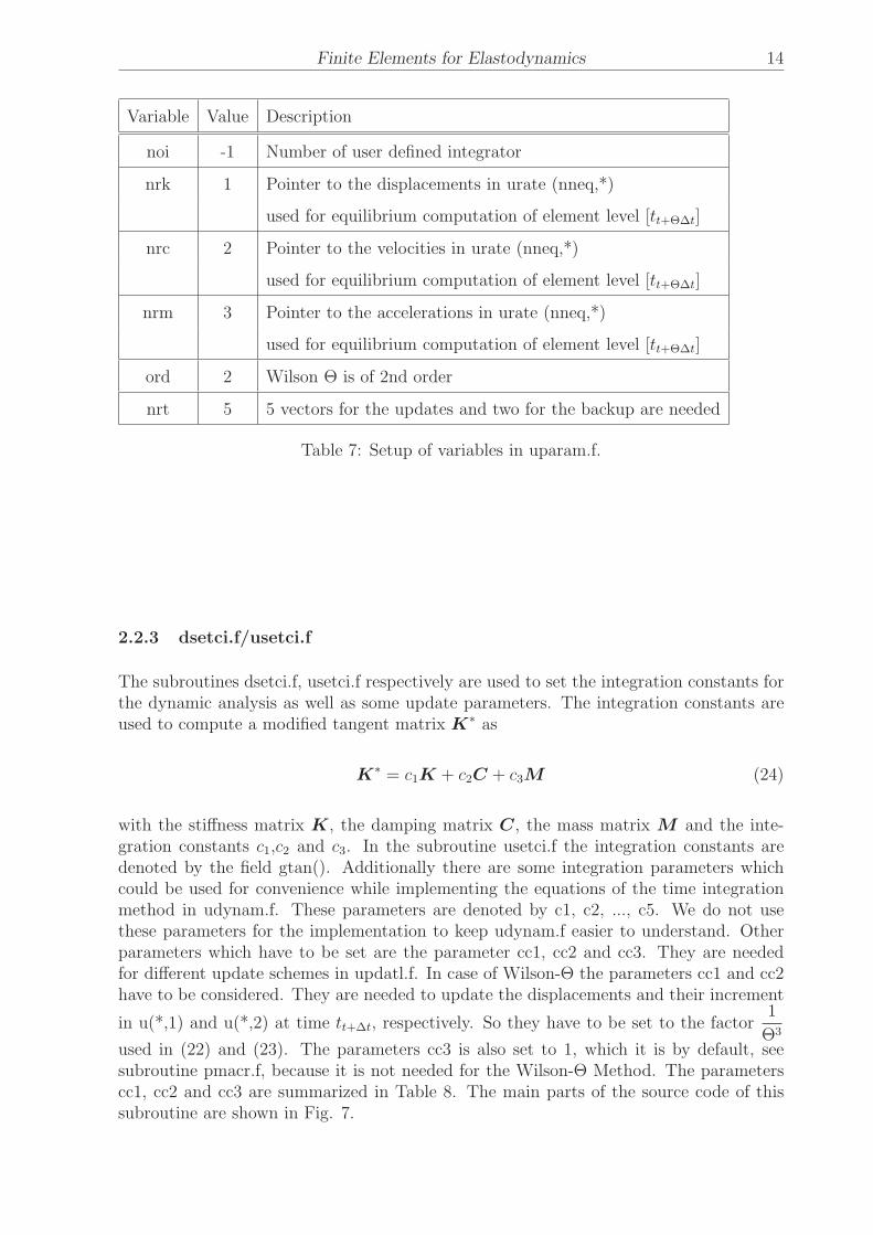
Finite Elements for Elastodynamics 14
Variable Value Description
noi -1 Number of user defined integrator
nrk 1 Pointer to the displacements in urate (nneq,*)
used for equilibrium computation of element level [tt+Θ∆t]
nrc 2 Pointer to the velocities in urate (nneq,*)
used for equilibrium computation of element level [tt+Θ∆t]
nrm 3 Pointer to the accelerations in urate (nneq,*)
used for equilibrium computation of element level [tt+Θ∆t]
ord 2 Wilson Θ is of 2nd order
nrt 5 5 vectors for the updates and two for the backup are needed
Table 7: Setup of variables in uparam.f.
2.2.3 dsetci.f/usetci.f
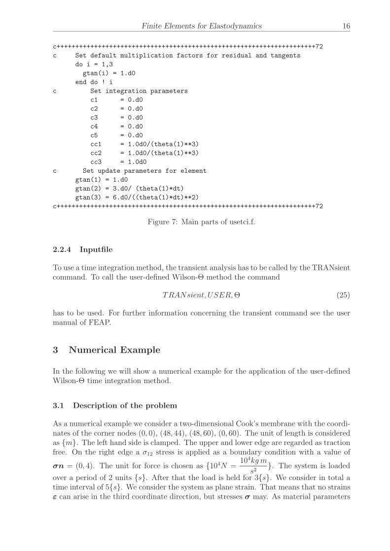
The subroutines dsetci.f, usetci.f respectively are used to set the integration constants forthe dynamic analysis as well as some update parameters. The integration constants areused to compute a modified tangent matrix K
∗ as
K∗ = c1K + c2C + c3M (24)
with the stiffness matrix K, the damping matrix C, the mass matrix M and the inte-gration constants c1,c2 and c3. In the subroutine usetci.f the integration constants aredenoted by the field gtan(). Additionally there are some integration parameters whichcould be used for convenience while implementing the equations of the time integrationmethod in udynam.f. These parameters are denoted by c1, c2, ..., c5. We do not usethese parameters for the implementation to keep udynam.f easier to understand. Otherparameters which have to be set are the parameter cc1, cc2 and cc3. They are neededfor different update schemes in updatl.f. In case of Wilson-Θ the parameters cc1 and cc2have to be considered. They are needed to update the displacements and their increment
in u(*,1) and u(*,2) at time tt+∆t, respectively. So they have to be set to the factor1
Θ3
used in (22) and (23). The parameters cc3 is also set to 1, which it is by default, seesubroutine pmacr.f, because it is not needed for the Wilson-Θ Method. The parameterscc1, cc2 and cc3 are summarized in Table 8. The main parts of the source code of thissubroutine are shown in Fig. 7.
K. Steeger 15
elseif(isw.eq.1) then
c noi := Number of the specific integrator
noi = -1
c nrk - Vector storing displacement vector for equilibrium computation
nrk = 1
c nrc - Vector storing velocity vector for equilibrium computation
nrc = 2
c nrm - Vector storing acceleration vector for equilibrium computation
nrm = 3
c ord - Order of ODE for this integrator
ord = 2
c nrt - Total vectors required by algorithm
nrt = 5
c Ensure that theta is not 0
if(ct(1).eq.0.0d0) ct(1) = 1.37
c Define parameter ct(3) for factor alpha in dparam.f
ct(3) = ct(1)
ct(2) = 0.d0
c+++++++++++++++++++++++++++++++++++++++++++++++++++++++++++++++++++++72
endif
c+++++++++++++++++++++++++++++++++++++++++++++++++++++++++++++++++++++72
Figure 6: Main parts of uparam.f.
Variable Description
cc1 Parameter to update the solution at tt+∆t
cc2 Parameter to update the increment at tt+∆t
cc3 Parameter to update specified boundary displacement
not needed for the Wilson-Θ Method
Table 8: Parameters cc1, cc2 and cc3.
Finite Elements for Elastodynamics 16
c+++++++++++++++++++++++++++++++++++++++++++++++++++++++++++++++++++++72
c Set default multiplication factors for residual and tangents
do i = 1,3
gtan(i) = 1.d0
end do ! i
c Set integration parameters
c1 = 0.d0
c2 = 0.d0
c3 = 0.d0
c4 = 0.d0
c5 = 0.d0
cc1 = 1.0d0/(theta(1)**3)
cc2 = 1.0d0/(theta(1)**3)
cc3 = 1.0d0
c Set update parameters for element
gtan(1) = 1.d0
gtan(2) = 3.d0/ (theta(1)*dt)
gtan(3) = 6.d0/((theta(1)*dt)**2)
c+++++++++++++++++++++++++++++++++++++++++++++++++++++++++++++++++++++72
Figure 7: Main parts of usetci.f.
2.2.4 Inputfile
To use a time integration method, the transient analysis has to be called by the TRANsientcommand. To call the user-defined Wilson-Θ method the command
TRANsient, USER, Θ (25)
has to be used. For further information concerning the transient command see the usermanual of FEAP.
3 Numerical Example
In the following we will show a numerical example for the application of the user-definedWilson-Θ time integration method.
3.1 Description of the problem
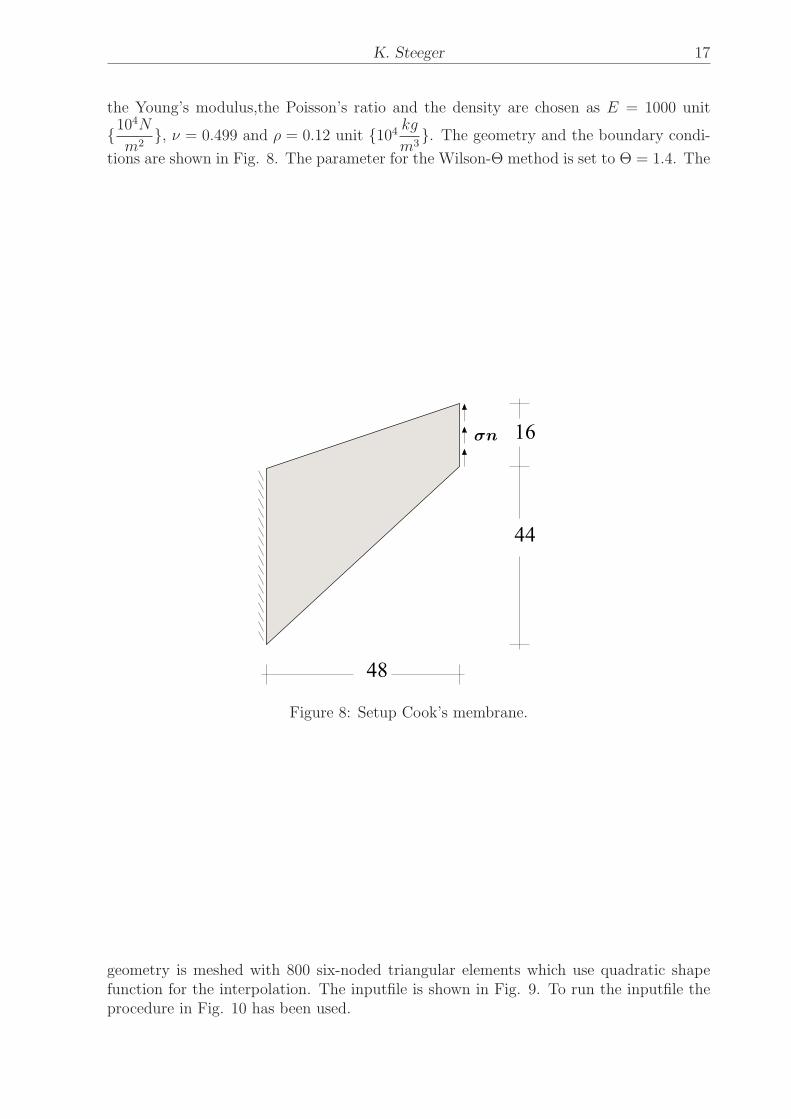
As a numerical example we consider a two-dimensional Cook’s membrane with the coordi-nates of the corner nodes (0, 0), (48, 44), (48, 60), (0, 60). The unit of length is consideredas {m}. The left hand side is clamped. The upper and lower edge are regarded as tractionfree. On the right edge a σ12 stress is applied as a boundary condition with a value of
σn = (0, 4). The unit for force is chosen as {104N =104kg m
s2}. The system is loaded
over a period of 2 units {s}. After that the load is held for 3{s}. We consider in total atime interval of 5{s}. We consider the system as plane strain. That means that no strainsε can arise in the third coordinate direction, but stresses σ may. As material parameters
K. Steeger 17
the Young’s modulus,the Poisson’s ratio and the density are chosen as E = 1000 unit
{104N
m2}, ν = 0.499 and ρ = 0.12 unit {104
kg
m3}. The geometry and the boundary condi-
tions are shown in Fig. 8. The parameter for the Wilson-Θ method is set to Θ = 1.4. The
16
44
48
σn
Figure 8: Setup Cook’s membrane.
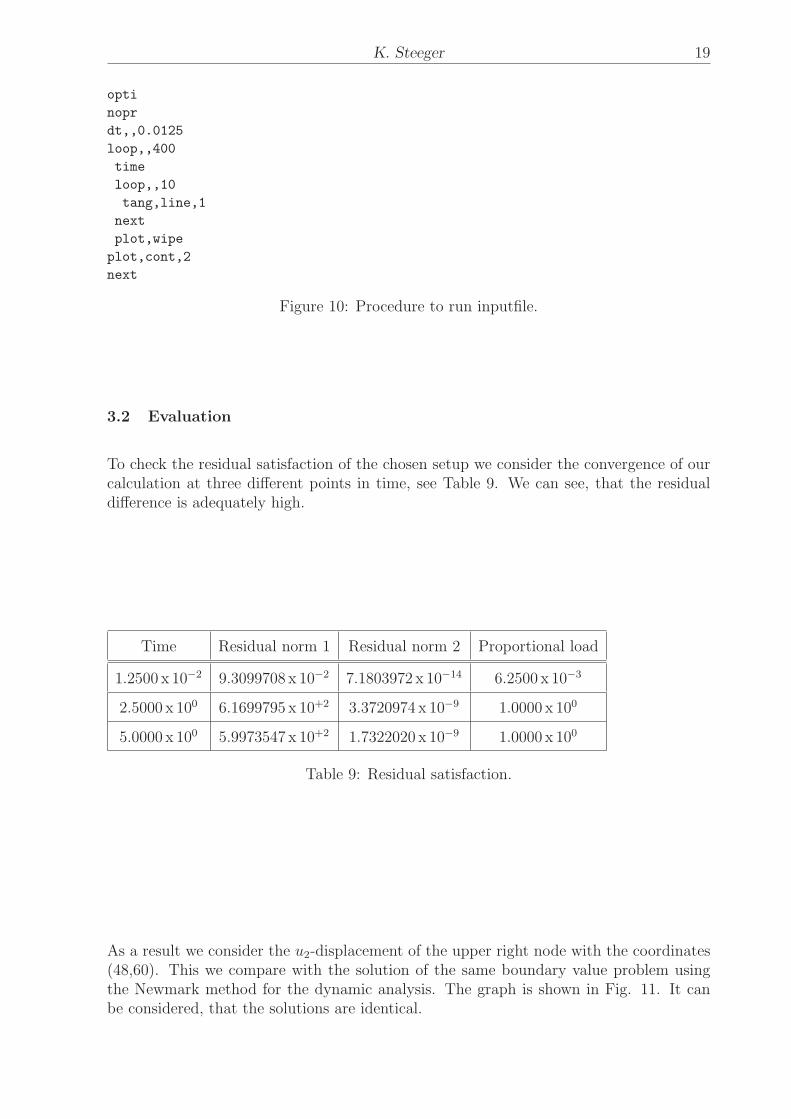
geometry is meshed with 800 six-noded triangular elements which use quadratic shapefunction for the interpolation. The inputfile is shown in Fig. 9. To run the inputfile theprocedure in Fig. 10 has been used.
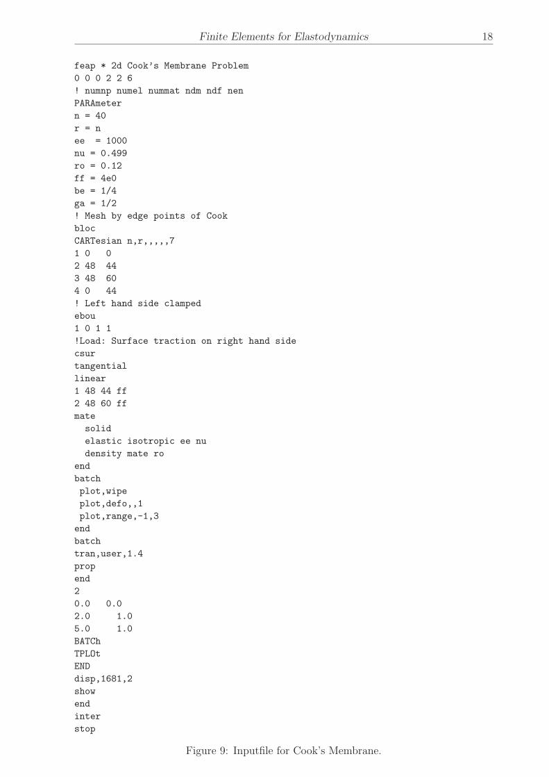
Finite Elements for Elastodynamics 18
feap * 2d Cook’s Membrane Problem
0 0 0 2 2 6
! numnp numel nummat ndm ndf nen
PARAmeter
n = 40
r = n
ee = 1000
nu = 0.499
ro = 0.12
ff = 4e0
be = 1/4
ga = 1/2
! Mesh by edge points of Cook
bloc
CARTesian n,r,,,,,7
1 0 0
2 48 44
3 48 60
4 0 44
! Left hand side clamped
ebou
1 0 1 1
!Load: Surface traction on right hand side
csur
tangential
linear
1 48 44 ff
2 48 60 ff
mate
solid
elastic isotropic ee nu
density mate ro
end
batch
plot,wipe
plot,defo,,1
plot,range,-1,3
end
batch
tran,user,1.4
prop
end
2
0.0 0.0
2.0 1.0
5.0 1.0
BATCh
TPLOt
END
disp,1681,2
show
end
inter
stop
Figure 9: Inputfile for Cook’s Membrane.
K. Steeger 19
opti
nopr
dt,,0.0125
loop,,400
time
loop,,10
tang,line,1
next
plot,wipe
plot,cont,2
next
Figure 10: Procedure to run inputfile.
3.2 Evaluation
To check the residual satisfaction of the chosen setup we consider the convergence of ourcalculation at three different points in time, see Table 9. We can see, that the residualdifference is adequately high.
Time Residual norm 1 Residual norm 2 Proportional load
1.2500 x 10⁻² 9.3099708 x 10⁻² 7.1803972 x 10⁻¹⁴ 6.2500 x 10⁻³
2.5000 x 100 6.1699795 x 10+2 3.3720974 x 10⁻⁹ 1.0000 x 100
5.0000 x 100 5.9973547 x 10+2 1.7322020 x 10⁻⁹ 1.0000 x 100
Table 9: Residual satisfaction.
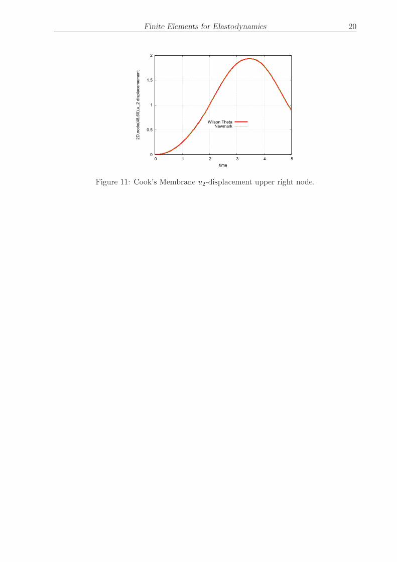
As a result we consider the u2-displacement of the upper right node with the coordinates(48,60). This we compare with the solution of the same boundary value problem usingthe Newmark method for the dynamic analysis. The graph is shown in Fig. 11. It canbe considered, that the solutions are identical.
Finite Elements for Elastodynamics 20
0
0.5
1
1.5
2
0 1 2 3 4 5
2D
,no
de
(48
,60
),u
_2
dis
pla
ce
me
me
nt
time
Wilson ThetaNewmark
Figure 11: Cook’s Membrane u2-displacement upper right node.
K. Steeger 21
References
I. Gladwell and R. Thomas. Stability properties of the newmark, houbolt and wilson θ methods. Int. J.
for num. and anal. meth. in geomech., Vol. 4:143–158, 1980.
T.J.R. Hughes. The Finite Element Method. Prentice-Hall Inc, New Jersey, 1987.
E.L. Wilson, I. Farhoomand, and K.J. Bathe. Nonlinear dynamic analysis of complex structures. Earth-
quake Engineering and Structural Dynamics., Vol. 1:241–252, 1973.