HAL Id: hal-01909526https://hal.archives-ouvertes.fr/hal-01909526

Submitted on 14 Dec 2018

HAL is a multi-disciplinary open accessarchive for the deposit and dissemination of sci-entific research documents, whether they are pub-lished or not. The documents may come fromteaching and research institutions in France orabroad, or from public or private research centers.

L’archive ouverte pluridisciplinaire HAL, estdestinée au dépôt et à la diffusion de documentsscientifiques de niveau recherche, publiés ou non,émanant des établissements d’enseignement et derecherche français ou étrangers, des laboratoirespublics ou privés.

Impact of Bolivian paleolake evaporation on the δ18O ofthe Andean glaciers during the last deglaciation(18.5–11.7 ka): diatom-inferred δ18O values and

hydro-isotopic modelingBenjamin Quesada, Florence Sylvestre, Françoise Vimeux, Jessica Black,Christine Paillès, Corinne Sonzogni, Anne Alexandre, Pierre-Henri Blard,

Alain Tonetto, Jean-Charles Mazur, et al.

To cite this version:Benjamin Quesada, Florence Sylvestre, Françoise Vimeux, Jessica Black, Christine Paillès, et al..Impact of Bolivian paleolake evaporation on the δ18O of the Andean glaciers during the last deglacia-tion (18.5–11.7 ka): diatom-inferred δ18O values and hydro-isotopic modeling. Quaternary ScienceReviews, Elsevier, 2015, 120, pp.93-106. �10.1016/j.quascirev.2015.04.022�. �hal-01909526�

lable at ScienceDirect

Quaternary Science Reviews 120 (2015) 93e106

Contents lists avai

Quaternary Science Reviews

journal homepage: www.elsevier .com/locate/quascirev

Impact of Bolivian paleolake evaporation on the d18O of the Andeanglaciers during the last deglaciation (18.5e11.7 ka): diatom-inferredd18O values and hydro-isotopic modeling

Benjamin Quesada a, b, *, Florence Sylvestre a, **, Françoise Vimeux b, c, Jessica Black a,Christine Paill�es a, Corinne Sonzogni a, Anne Alexandre a, Pierre-Henri Blard d,Alain Tonetto e, Jean-Charles Mazur a, H�el�ene Bruneton a

a Aix-Marseille Universit�e, CNRS, IRD, CEREGE, UM 34, Europole de l'Arbois, BP 80, 13545 Aix en Provence Cedex 04, Franceb Institut Pierre Simon Laplace (IPSL), Laboratoire des Sciences de Climat et de l'Environnement (LSCE), UMR 8212 (CEA-CNRS-UVSQ), CEA Saclay,Orme des Merisiers, Bat. 701, 91191 Gif-sur-Yvette, Francec Laboratoire HydroSciences Montpellier (HSM), UMR 5569 (CNRS-IRD-UM1-UM2), 34095 Montpellier, Franced Centre de Recherches P�etrographiques et G�eochimiques (CRPG), UMR 7358, CNRS, Nancy-Universit�e, Vandœuvre-l�es-Nancy, Francee Aix-Marseille Universit�e, PRATIM, F�ed�eration de Chimie, 3 Place Victor Hugo, 13331 Marseille Cedex 3, France

a r t i c l e i n f o

Article history:Received 7 November 2014Received in revised form27 April 2015Accepted 28 April 2015Available online 22 May 2015

Keywords:Bolivian AltiplanoDeglaciationPaleolakesAndean ice coresDiatomsOstracodsOxygen isotopes

* Corresponding author. Aix-Marseille Universit�e,Europole de l'Arbois, BP 80, 13545 Aix en Provence C** Corresponding author.

E-mail addresses: benjamin.quesada@kit.edu (B. Q(F. Sylvestre).

http://dx.doi.org/10.1016/j.quascirev.2015.04.0220277-3791/© 2015 Elsevier Ltd. All rights reserved.

a b s t r a c t

During the last deglaciation, the Bolivian Altiplano (15e23�S, 66e70�W) was occupied by paleolakeTauca covering, at least, ~51,000 km2 at its maximum highstand between 16.5 and 15 ka. Twenty-fivehundred years later, after a massive regression, a new transgressive phase, produced paleolake Coi-pasa, smaller than Tauca and restricted to the southern part of the basin. These paleolakes were over-looked at the west by the Sajama ice cap. The latter provides a continuous record of the oxygen isotopiccomposition of paleo-precipitation for the last 25 ka. Contemporaneously to the end of paleolake Tauca,around 14.3 ka, the Sajama ice cap recorded a significant increase in ice oxygen isotopic composition(d18Oice). This paper examines to what extent the disappearance of Lake Tauca contributed to precipi-tation on the Sajama summit and this specific isotopic variation. The water d18O values of paleolakesTauca and Coipasa (d18Olake) were quantitatively reconstructed from 18.5 to 11.7 ka based on diatomisotopic composition (d18Odiatoms) and ostracod isotopic composition (d18Ocarbonates) retrieved in lacus-trine sediments. At a centennial time scale, a strong trend appears: abrupt decreases of d18Olake duringlake fillings are immediately followed by abrupt increases of d18Olake during lake level stable phases. Thehighest variation occurred at ~15.8 ka with a d18Olake decrease of about ~10‰, concomitant with the LakeTauca highstand, followed ~400 years later by a 7‰ increase in d18Olake. A simple hydro-isotopicmodeling approach reproduces consistently this rapid “decreaseeincrease” feature. Moreover, it sug-gests that this unexpected re-increase in d18Olake after filling phases can be partly explained by anequilibration of isotopic fluxes during the lake steady-state. Based on isotopic calculations during lakeevaporation and a simple water stable isotopes balance between potential moisture sources at Sajama(advection versus lake evaporation), we show that total or partial evaporation (from 5 to 60%) of pale-olake Tauca during its major regression phase at 14.3 ka could explain the pronounced isotopic excursionat Sajama ice cap. These results suggest that perturbations of the local hydrological cycle in lacustrineareas may substantially affect the paleoclimatic interpretation of the near-by isotopic signals (e.g. ice coreor speleothems).

© 2015 Elsevier Ltd. All rights reserved.

CNRS, IRD, CEREGE, UM 34,edex 04, France.

uesada), sylvestre@cerege.fr

1. Introduction

The isotopic composition of continental sedimentary and icearchives has long been used to infer past climate variability. Toreconstruct reliable paleoclimate information, it is necessary to

B. Quesada et al. / Quaternary Science Reviews 120 (2015) 93e10694

translate geochemical signals into quantified climate parameters.Within this framework, any environmental or climate processaffecting the isotopic composition of climate archives must betracked. In particular, continental water recycling involves frac-tionating and non-fractionating processes whose magnitudes haveto be defined at the regional scale. In this paper, we examine theimpact of such processes over the Bolivian Altiplano, which offers aunique opportunity to study the recycling moisture from a localsource.

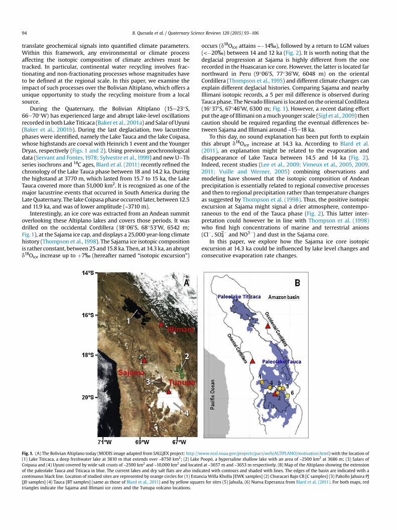
During the Quaternary, the Bolivian Altiplano (15e23�S,66e70�W) has experienced large and abrupt lake-level oscillationsrecorded in both Lake Titicaca (Baker et al., 2001a) and Salar of Uyuni(Baker et al., 2001b). During the last deglaciation, two lacustrinephases were identified, namely the Lake Tauca and the lake Coipasa,whose highstands are coeval with Heinrich 1 event and the YoungerDryas, respectively (Figs. 1 and 2). Using previous geochronologicaldata (Servant and Fontes, 1978; Sylvestre et al., 1999) and new UeThseries isochrons and 14C ages, Blard et al. (2011) recently refined thechronology of the Lake Tauca phase between 18 and 14.2 ka. Duringthe highstand at 3770 m, which lasted from 15.7 to 15 ka, the LakeTauca covered more than 51,000 km2. It is recognized as one of themajor lacustrine events that occurred in South America during theLateQuaternary. The lake Coipasa phase occurred later, between12.5and 11.9 ka, and was of lower amplitude (~3710 m).

Interestingly, an ice core was extracted from an Andean summitoverlooking these Altiplano lakes and covers those periods. It wasdrilled on the occidental Cordillera (18�060S, 68�530W, 6542 m;Fig. 1), at the Sajama ice cap, and displays a 25,000 year-long climatehistory (Thompson et al., 1998). The Sajama ice isotopic compositionis rather constant, between 25and15.8 ka. Then, at 14.3 ka, an abruptd18Oice increase up to þ7‰ (hereafter named “isotopic excursion”)

Fig. 1. (A) The Bolivian Altiplano today (MODIS image adapted from SALLJEX project: http://w(1) Lake Titicaca, a deep freshwater lake at 3810 m that extends over ~8750 km2; (2) LakeCoipasa and (4) Uyuni covered by wide salt crusts of ~2500 km2 and ~10,000 km2 and locateof the paleolake Tauca and Titicaca in blue. The current lakes and dry salt flats are also indicontinuous black line. Location of studied sites are represented by orange circles for (1) Estan[J0 samples] (4) Tauca [BT samples] (same as those of Blard et al., 2011) and by yellow squartriangles indicate the Sajama and Illimani ice cores and the Tunupa volcano locations.

occurs (d18Oice attains ~�14‰), followed by a return to LGM values(<�20‰) between 14 and 12 ka (Fig. 2). It is worth noting that thedeglacial progression at Sajama is highly different from the onerecorded in the Huascaran ice core. However, the latter is located farnorthward in Peru (9�060S, 77�360W, 6048 m) on the orientalCordillera (Thompson et al., 1995) and different climate changes canexplain different deglacial histories. Comparing Sajama and nearbyIllimani isotopic records, a 5 per mil difference is observed duringTauca phase. TheNevado Illimani is located on the oriental Cordillera(16�370S, 67�460W, 6300 m; Fig. 1). However, a recent dating effortput the age of Illimani on amuchyounger scale (Sigl et al., 2009) thencaution should be required regarding the eventual differences be-tween Sajama and Illimani around ~15e18 ka.

To this day, no sound explanation has been put forth to explainthis abrupt d18Oice increase at 14.3 ka. According to Blard et al.(2011), an explanation might be related to the evaporation anddisappearance of Lake Tauca between 14.5 and 14 ka (Fig. 2).Indeed, recent studies (Lee et al., 2009; Vimeux et al., 2005, 2009,2011; Vuille and Werner, 2005) combining observations andmodeling have showed that the isotopic composition of Andeanprecipitation is essentially related to regional convective processesand then to regional precipitation rather than temperature changesas suggested by Thompson et al. (1998). Thus, the positive isotopicexcursion at Sajama might signal a drier atmosphere, contempo-raneous to the end of the Tauca phase (Fig. 2). This latter inter-pretation could however be in line with Thompson et al. (1998)who find high concentrations of marine and terrestrial anions(Cl�, SO4

2� and NO3�) and dust in the Sajama core.In this paper, we explore how the Sajama ice core isotopic

excursion at 14.3 ka could be influenced by lake level changes andconsecutive evaporation rate changes.

ww.nssl.noaa.gov/projects/pacs/web/ALTIPLANO/motivation.html) with the location ofPoop�o, a hypersaline shallow lake with an area of ~2500 km2 at 3686 m; (3) Salars ofd at ~3657 m and ~3653 m respectively. (B) Map of the Altiplano showing the extensioncated with contours and shaded with lines. The edges of the basin are indicated with acia Willa Khollu [EWK samples] (2) Churacari Bajo CB [C samples] (3) Pakollo Jahuira PJes for sites (5) Jahuila, (6) Nueva Esperanza from Blard et al. (2011). For both maps, red

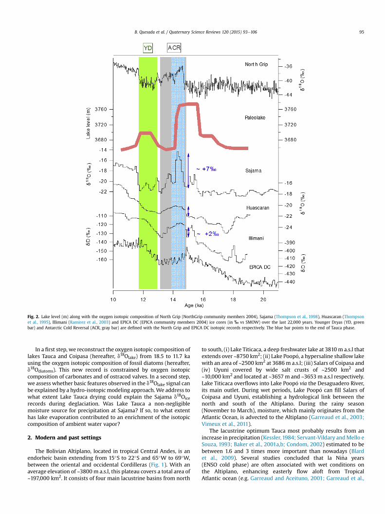
Fig. 2. Lake level (m) along with the oxygen isotopic composition of North Grip (NorthGrip community members 2004), Sajama (Thompson et al., 1998), Huascaran (Thompsonet al., 1995), Illimani (Ramirez et al., 2003) and EPICA DC (EPICA community members 2004) ice cores (in ‰ vs SMOW) over the last 22,000 years. Younger Dryas (YD, greenbar) and Antarctic Cold Reversal (ACR, gray bar) are defined with the North Grip and EPICA DC isotopic records respectively. The blue bar points to the end of Tauca phase.

B. Quesada et al. / Quaternary Science Reviews 120 (2015) 93e106 95

In a first step, we reconstruct the oxygen isotopic composition oflakes Tauca and Coipasa (hereafter, d18Olake) from 18.5 to 11.7 kausing the oxygen isotopic composition of fossil diatoms (hereafter,d18Odiatoms). This new record is constrained by oxygen isotopiccomposition of carbonates and of ostracod valves. In a second step,we assess whether basic features observed in the d18Olake signal canbe explained by a hydro-isotopic modeling approach.We address towhat extent Lake Tauca drying could explain the Sajama d18Oicerecords during deglaciation. Was Lake Tauca a non-negligiblemoisture source for precipitation at Sajama? If so, to what extenthas lake evaporation contributed to an enrichment of the isotopiccomposition of ambient water vapor?

2. Modern and past settings

The Bolivian Altiplano, located in tropical Central Andes, is anendorheic basin extending from 15�S to 22�S and 65�W to 69�W,between the oriental and occidental Cordilleras (Fig. 1). With anaverage elevation of ~3800m a.s.l, this plateau covers a total area of~197,000 km2. It consists of four main lacustrine basins from north

to south, (i) Lake Titicaca, a deep freshwater lake at 3810m a.s.l thatextends over ~8750 km2; (ii) Lake Poop�o, a hypersaline shallow lakewith an area of ~2500 km2 at 3686m a.s.l; (iii) Salars of Coipasa and(iv) Uyuni covered by wide salt crusts of ~2500 km2 and~10,000 km2 and located at ~3657m and ~3653 m a.s.l respectively.Lake Titicaca overflows into Lake Poop�o via the Desaguadero River,its main outlet. During wet periods, Lake Poop�o can fill Salars ofCoipasa and Uyuni, establishing a hydrological link between thenorth and south of the Altiplano. During the rainy season(November to March), moisture, which mainly originates from theAtlantic Ocean, is advected to the Altiplano (Garreaud et al., 2003;Vimeux et al., 2011).

The lacustrine optimum Tauca most probably results from anincrease in precipitation (Kessler,1984; Servant-Vildary andMello eSouza, 1993; Baker et al., 2001a,b; Condom, 2002) estimated to bebetween 1.6 and 3 times more important than nowadays (Blardet al., 2009). Several studies concluded that la Ni~na years(ENSO cold phase) are often associated with wet conditions onthe Altiplano, enhancing easterly flow aloft from TropicalAtlantic ocean (e.g. Garreaud and Aceituno, 2001; Garreaud et al.,

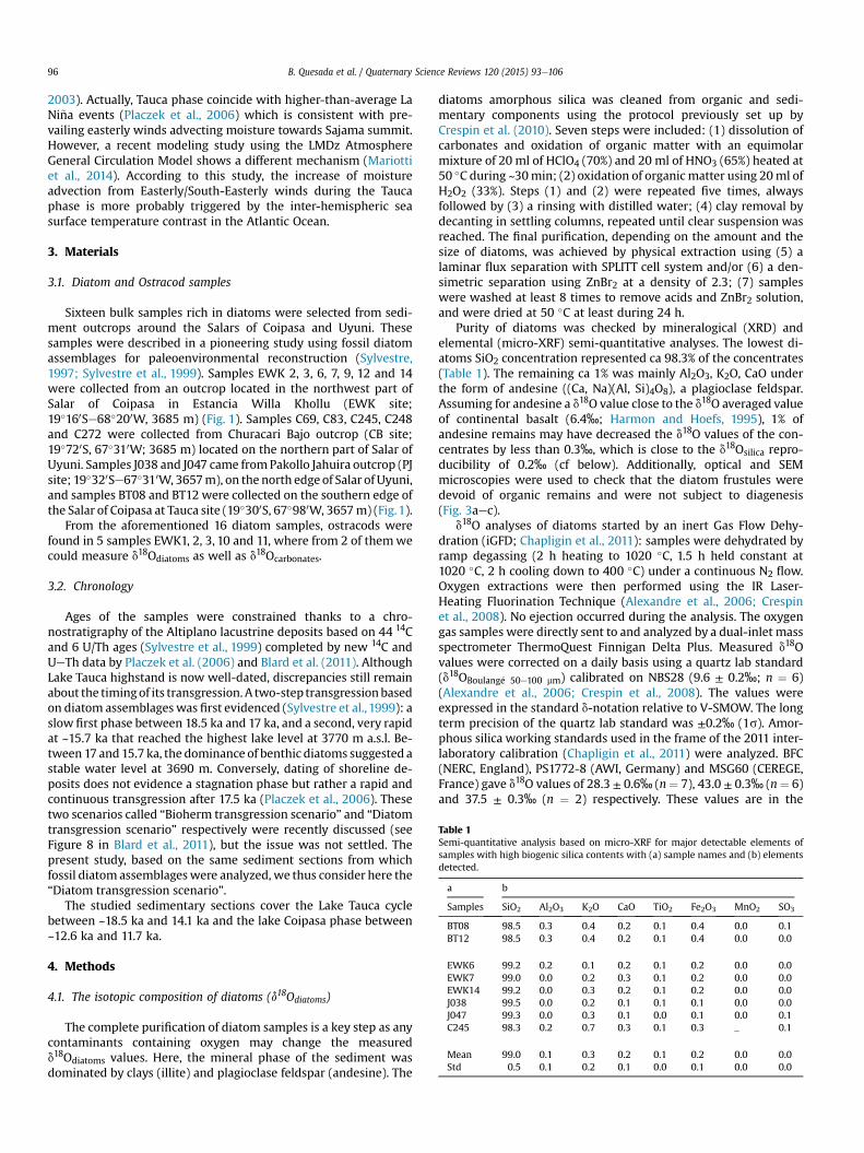
Table 1Semi-quantitative analysis based on micro-XRF for major detectable elements ofsamples with high biogenic silica contents with (a) sample names and (b) elementsdetected.

a b

Samples SiO2 Al2O3 K2O CaO TiO2 Fe2O3 MnO2 SO3

BT08 98.5 0.3 0.4 0.2 0.1 0.4 0.0 0.1BT12 98.5 0.3 0.4 0.2 0.1 0.4 0.0 0.0

EWK6 99.2 0.2 0.1 0.2 0.1 0.2 0.0 0.0EWK7 99.0 0.0 0.2 0.3 0.1 0.2 0.0 0.0EWK14 99.2 0.0 0.3 0.2 0.1 0.2 0.0 0.0J038 99.5 0.0 0.2 0.1 0.1 0.1 0.0 0.0J047 99.3 0.0 0.3 0.1 0.0 0.1 0.0 0.1C245 98.3 0.2 0.7 0.3 0.1 0.3 _ 0.1

Mean 99.0 0.1 0.3 0.2 0.1 0.2 0.0 0.0Std 0.5 0.1 0.2 0.1 0.0 0.1 0.0 0.0

B. Quesada et al. / Quaternary Science Reviews 120 (2015) 93e10696

2003). Actually, Tauca phase coincide with higher-than-average LaNi~na events (Placzek et al., 2006) which is consistent with pre-vailing easterly winds advecting moisture towards Sajama summit.However, a recent modeling study using the LMDz AtmosphereGeneral Circulation Model shows a different mechanism (Mariottiet al., 2014). According to this study, the increase of moistureadvection from Easterly/South-Easterly winds during the Taucaphase is more probably triggered by the inter-hemispheric seasurface temperature contrast in the Atlantic Ocean.

3. Materials

3.1. Diatom and Ostracod samples

Sixteen bulk samples rich in diatoms were selected from sedi-ment outcrops around the Salars of Coipasa and Uyuni. Thesesamples were described in a pioneering study using fossil diatomassemblages for paleoenvironmental reconstruction (Sylvestre,1997; Sylvestre et al., 1999). Samples EWK 2, 3, 6, 7, 9, 12 and 14were collected from an outcrop located in the northwest part ofSalar of Coipasa in Estancia Willa Khollu (EWK site;19�160Se68�200W, 3685 m) (Fig. 1). Samples C69, C83, C245, C248and C272 were collected from Churacari Bajo outcrop (CB site;19�720S, 67�310W; 3685 m) located on the northern part of Salar ofUyuni. Samples J038 and J047 came fromPakollo Jahuira outcrop (PJsite; 19�320Se67�310W, 3657m), on the north edge of Salar of Uyuni,and samples BT08 and BT12 were collected on the southern edge ofthe Salar of Coipasa at Tauca site (19�300S, 67�980W, 3657m) (Fig.1).

From the aforementioned 16 diatom samples, ostracods werefound in 5 samples EWK1, 2, 3, 10 and 11, where from 2 of themwecould measure d18Odiatoms as well as d18Ocarbonates.

3.2. Chronology

Ages of the samples were constrained thanks to a chro-nostratigraphy of the Altiplano lacustrine deposits based on 44 14Cand 6 U/Th ages (Sylvestre et al., 1999) completed by new 14C andUeTh data by Placzek et al. (2006) and Blard et al. (2011). AlthoughLake Tauca highstand is now well-dated, discrepancies still remainabout the timingof its transgression. A two-step transgressionbasedon diatom assemblageswas first evidenced (Sylvestre et al., 1999): aslow first phase between 18.5 ka and 17 ka, and a second, very rapidat ~15.7 ka that reached the highest lake level at 3770 m a.s.l. Be-tween 17 and 15.7 ka, the dominance of benthic diatoms suggested astable water level at 3690 m. Conversely, dating of shoreline de-posits does not evidence a stagnation phase but rather a rapid andcontinuous transgression after 17.5 ka (Placzek et al., 2006). Thesetwo scenarios called “Bioherm transgression scenario” and “Diatomtransgression scenario” respectively were recently discussed (seeFigure 8 in Blard et al., 2011), but the issue was not settled. Thepresent study, based on the same sediment sections from whichfossil diatom assemblageswere analyzed, we thus consider here the“Diatom transgression scenario”.

The studied sedimentary sections cover the Lake Tauca cyclebetween ~18.5 ka and 14.1 ka and the lake Coipasa phase between~12.6 ka and 11.7 ka.

4. Methods

4.1. The isotopic composition of diatoms (d18Odiatoms)

The complete purification of diatom samples is a key step as anycontaminants containing oxygen may change the measuredd18Odiatoms values. Here, the mineral phase of the sediment wasdominated by clays (illite) and plagioclase feldspar (andesine). The

diatoms amorphous silica was cleaned from organic and sedi-mentary components using the protocol previously set up byCrespin et al. (2010). Seven steps were included: (1) dissolution ofcarbonates and oxidation of organic matter with an equimolarmixture of 20 ml of HClO4 (70%) and 20 ml of HNO3 (65%) heated at50 �C during ~30min; (2) oxidation of organicmatter using 20ml ofH2O2 (33%). Steps (1) and (2) were repeated five times, alwaysfollowed by (3) a rinsing with distilled water; (4) clay removal bydecanting in settling columns, repeated until clear suspension wasreached. The final purification, depending on the amount and thesize of diatoms, was achieved by physical extraction using (5) alaminar flux separation with SPLITT cell system and/or (6) a den-simetric separation using ZnBr2 at a density of 2.3; (7) sampleswere washed at least 8 times to remove acids and ZnBr2 solution,and were dried at 50 �C at least during 24 h.

Purity of diatoms was checked by mineralogical (XRD) andelemental (micro-XRF) semi-quantitative analyses. The lowest di-atoms SiO2 concentration represented ca 98.3% of the concentrates(Table 1). The remaining ca 1% was mainly Al2O3, K2O, CaO underthe form of andesine ((Ca, Na)(Al, Si)4O8), a plagioclase feldspar.Assuming for andesine a d18O value close to the d18O averaged valueof continental basalt (6.4‰; Harmon and Hoefs, 1995), 1% ofandesine remains may have decreased the d18O values of the con-centrates by less than 0.3‰, which is close to the d18Osilica repro-ducibility of 0.2‰ (cf below). Additionally, optical and SEMmicroscopies were used to check that the diatom frustules weredevoid of organic remains and were not subject to diagenesis(Fig. 3aec).

d18O analyses of diatoms started by an inert Gas Flow Dehy-dration (iGFD; Chapligin et al., 2011): samples were dehydrated byramp degassing (2 h heating to 1020 �C, 1.5 h held constant at1020 �C, 2 h cooling down to 400 �C) under a continuous N2 flow.Oxygen extractions were then performed using the IR Laser-Heating Fluorination Technique (Alexandre et al., 2006; Crespinet al., 2008). No ejection occurred during the analysis. The oxygengas samples were directly sent to and analyzed by a dual-inlet massspectrometer ThermoQuest Finnigan Delta Plus. Measured d18Ovalues were corrected on a daily basis using a quartz lab standard(d18OBoulang�e 50e100 mm) calibrated on NBS28 (9.6 ± 0.2‰; n ¼ 6)(Alexandre et al., 2006; Crespin et al., 2008). The values wereexpressed in the standard d-notation relative to V-SMOW. The longterm precision of the quartz lab standard was ±0.2‰ (1s). Amor-phous silica working standards used in the frame of the 2011 inter-laboratory calibration (Chapligin et al., 2011) were analyzed. BFC(NERC, England), PS1772-8 (AWI, Germany) and MSG60 (CEREGE,France) gave d18O values of 28.3 ± 0.6‰ (n¼ 7), 43.0 ± 0.3‰ (n¼ 6)and 37.5 ± 0.3‰ (n ¼ 2) respectively. These values are in the

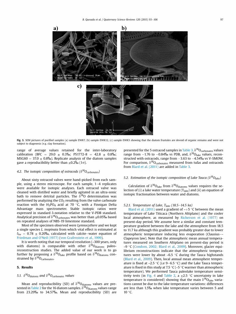
Fig. 3. SEM pictures of purified samples (a) sample EWK7, (b) sample EWK12, (c) sample EWK3 showing that the diatom frustules are devoid of organic remains and were notsubject to diagenesis (e.g. clay formation).

B. Quesada et al. / Quaternary Science Reviews 120 (2015) 93e106 97

range of average values retained for the inter-laboratorycalibration (BFC ¼ 29.0 ± 0.3‰; PS1772-8 ¼ 42.8 ± 0.8‰;MSG60 ¼ 37.0 ± 0.8‰). Replicate analysis of the diatom samplesgave a reproducibility better than ±0.2‰ (1s).

4.2. The isotopic composition of ostracods (d18Ocarbonates)

About sixty ostracod valves were hand-picked from each sam-ple, using a stereo microscope. For each sample, 1e4 replicateswere available for isotopic analyses. Each ostracod valve wascleaned with distilled water and briefly agitated in an ultra-sonicbath to remove detrital particles. The d18O determination wasperformed by analyzing the CO2 resulting from the valve carbonatereaction with the H3PO4 acid at 70 �C, with a Finnigan DeltaAdvantage mass spectrometer. Stable isotopic ratios wereexpressed in standard d-notation relative to the V-PDB standard.Analytical precision of d18Ocarbonates was better than ±0.05‰ basedon repeated analyses of NBS-19 limestone standard.

Most of the specimen observed were Lymnocythere and we kepta single species L. inopinata from which vital effect is estimated atdev ¼ 0.78 ± 0.20‰, calculated with calciteewater equation ofFriedman and O'Neil (1977) (von Grafenstein et al., 1999).

It is worth noting that our temporal resolution (~300 years, onlywith diatoms) is comparable with other d18Odiatoms paleo-reconstruction studies. The added value of our work is to gofurther by proposing a d18Olake profile based on d18Odiatoms con-strained by d18Ocarbonates.

5. Results

5.1. d18Odiatoms and d18Ocarbonates values

Mean and reproducibility (SD) of d18Odiatoms values are pre-sented in Table 2 for the 16 diatom samples. d18Odiatoms values rangefrom 23.29‰ to 34.57‰. Mean and reproducibility (SD) are

presented for the 5 ostracod samples in Table 3. d18Ocarbonates valuesrange from �1.76 to �0.84‰ vs PDB, and, d18Olake values, recon-structed with ostracods, range from �3.63 to �4.54‰ vs V-SMOW.For comparison, d18Ocarbonates measured from tufas and ostracodsfrom Blard et al. (2011) are added in Table 3.

5.2. Estimation of the isotopic composition of Lake Tauca (d18Olake)

Calculation of d18Olake from d18Odiatoms values requires the se-lection of (i) a lake water temperature (Tlake) and (ii) an equation ofisotopic fractionation between water and diatoms.

5.2.1. Temperature of Lake, Tlake (18.5e14.5 ka)Blard et al. (2011) used a gradient of ~þ5 �C between the mean

temperature of Lake Titicaca (Northern Altiplano) and the coolerlocal atmosphere, as measured by Richerson et al. (1977) onpresent-day period. We assume here a similar and constant tem-perature gradient between the lake and the atmosphere from 18.5to 11.7 ka although this gradient was probably greater due to loweratmospheric temperature inducing less evaporation (Clausiuse-Clapeyron law). Note that the atmospheric mean annual tempera-tures measured on Southern Altiplano on present-day period is~9 �C (Condom, 2002; Blard et al., 2009). Moreover, glacier equi-librium reconstructions indicate that the atmospheric tempera-tures were lower by about ~6.5 �C during the Tauca highstands(Blard et al., 2009). Then, local annual mean atmosphere temper-ature is fixed at ~2.5 �C (i.e 9e6.5 �C) and the Lake Tauca temper-ature is fixed in this study at 7.5 �C (~5 �Cwarmer than atmospherictemperature). We performed Tauca paleolake temperature sensi-tivity tests (in Fig. 4 and Table 2, a ±2.5 �C uncertainty in laketemperature is considered) showing that the main d18Olake varia-tions cannot be due to the lake temperature variations: differencesare less than 1.5‰ when lake temperature varies between 5 and10 �C.

Table 2Oxygen isotopic composition of diatom samples (d18Odiatoms): (a) sample names; (b) altitude of the studied site; (c) calibrated ages (ka) using IntCal09; (d) Mean, standarddeviation (SD) and number of replicates (n) of d18Odiatoms values; (e) d18Olake calculated using diatoms-water fractionation from Brandriss et al. (1998); (f) d18Olake calculatedusing diatoms-water fractionation from Moschen et al. (2005); (g) d18Olake calculated using corrected Ddiatoms-lake water vs Temperature calibration modified from Crespin et al.(2010) and Alexandre et al. (2012); (h) d18Olake calculated using diatoms-water fractionation from Dodd and Sharp (2010); (i) d18Olake calculated using quartzewater frac-tionation from Matsuhisa et al. (1979).

a b c d e f g h i

Samples Altitude(m a.s.l)

Calibratedage ka (±2s)

d18Odiatoms (‰ vs V-SMOW) d18Olake (‰ vsV-SMOW) afterBrandriss et al.(1998)

d18Olake (‰ vsV-SMOW) afterMoschen et al.(2005).

d18Olake (‰ vsV-SMOW) afterCrespin et al.(2010)

d18Olake (‰ vsV-SMOW) afterDodd and Sharp(2010)

d18Olake (‰ vsV-SMOW) afterMatsuhisa et al.(1979)

Mean SD n

BT08 3657 11.7 ± 0.1 33.90 0.10 2 �1.87 �1.01 0.66 �1.13 �5.40BT12 3657 12.6 ± 0.1 30.51 0.27 2 �5.25 �4.39 �2.73 �4.51 �8.78

EWK2 3685 14.2 ± 0.4 33.14 0.21 3 �2.62 �1.76 �0.10 �1.88 �6.15EWK3 3685 14.7 ± 0.5 31.80 0.01 2 �3.96 �3.11 �1.44 �3.23 �7.49C69 3685 15.2 ± 0.5 30.59 0.51 2 �5.17 �4.31 �2.65 �4.43 �8.70C83 3685 15.4 ± 0.5 23.29 0.05 2 �12.48 �11.62 �9.95 �11.74 �16.01EWK6 3685 15.6 ± 0.8 23.34 0.20 2 �12.42 �11.56 �9.90 �11.68 �15.95EWK7 3685 15.8 ± 0.8 33.22 0.27 3 �2.55 �1.69 �0.02 �1.81 �6.08EWK9 3685 16.3 ± 0.6 33.66 0.43 3 �2.10 �1.24 0.42 �1.36 �5.63EWK12 3685 16.8 ± 0.2 29.07 0.03 2 �6.69 �5.83 �4.17 �5.95 �10.22EWK14 3685 16.9 ± 0.2 33.91 0.02 2 �1.85 �0.99 0.67 �1.11 �5.38J038 3657 17.2 ± 0.4 34.57 0.31 4 �1.20 �0.34 1.33 �0.46 �4.73C245 3685 17.7 ± 0.3 31.53 0.17 2 �4.23 �3.38 �1.71 �3.50 �7.76J047 3657 18.1 ± 0.3 33.69 0.15 2 �2.07 �1.21 0.45 �1.33 �5.60C248 3685 18.2 ± 0.4 27.24 0.19 2 �8.52 �7.67 �6.00 �7.79 �12.05C272 3685 18.5 ± 0.1 24.80 0.19 2 �10.96 �10.11 �8.44 �10.23 �14.50

B. Quesada et al. / Quaternary Science Reviews 120 (2015) 93e10698

5.2.2. Equation of isotopic fractionation between diatoms and lakewater (d18Odiatoms � d18Olake ¼ a·Tlake þ b)

As diatom silica precipitates in isotopic equilibrium with lakewater (Leng and Barker, 2006), a thermo-dependent relationshipcan be expressed as [d18Odiatoms � d18Olake] (‰ vs V-SMOW)¼ a$Tlake (�C)þ b. According to previous calibration studies(Brandriss et al., 1998; Moschen et al., 2005; Crespin et al., 2010;Dodd and Sharp, 2010; Alexandre et al., 2012; Dodd et al., 2012),a is comprised between �0.2 and �0.3‰/�C, when b strongly dif-fers from one study to another, probably due to discrepancies inmethodological approaches (Crespin et al., 2010; Alexandre et al.,2012) or to early post-mortem diagenesis at the sedimentewaterinterface (Dodd and Sharp, 2010; Dodd et al., 2012). For this reason,Dodd and Sharp (2010) and Dodd et al. (2012) suggested the use ofthermo-dependent relationships measured for quartz rather thanthe ones measured for modern diatoms, for interpreting fossildiatom d18O records.

Table 3Oxygen isotopic composition of ostracod samples (d18Oostracods): (a) sample names; (b) creplicates (n) of d18Oostracods; (d) d18Olake calculated using the carbonateewater equation(2011) measured on 5 tufas and 1 ostracod (unknown vital effect) are included and reconsistency with our measurements. The carbonateewater fractionation is calculated co

a b c

Samples Calibrated age ka (±2s) d18Ocarbonates (‰ vs-PDB)

Mean SD

This studyEWK1 14.1 ± 0.2 �1.6 0.04EWK2 14.2 ± 0.4 �1.76 0.10EWK3 14.7 ± 0.5 �1.01 0.39EWK10 16.6 ± 0.4 �1.17 0.13EWK11 16.77 ± 0.4 �0.84 e

Data from Blard et al. (2011)Jah-14b 11.9 ± 0.2 �0.04 0.00Bo-93.26 12.8 ± 0.2 �0.17 0.01Jah-14a 14.6 ± 0.4 �0.91 0.01Hua-44 15.1 ± 0.5 �1.38 0.02Piv-Ostra 15.9 ± 0.6 �2.19 0.01Jah-12b 16.2 ± 0.5 �0.88 0.01

When estimated using the quartzewater relationship(Matsuhisa et al., 1979), d18Olake values were more 18O-depleted by4‰ than when estimated using the diatomewater relationship(Brandriss et al., 1998; Moschen et al., 2005; Crespin et al., 2010corrected in Alexandre et al., 2012; Dodd and Sharp, 2010)(Table 2). Indeed, the results showhighly depleted values estimatedfrom quartzewater fractionation of about �8.94‰ at 7.5 �Ccompared with those calculated with diatoms-water fractionation(average ¼ �4.39‰) (Table 2). We used carbonate-based d18Olakereconstruction between 16.8 and 14.2 ka BP (n ¼ 10, see Table 3)representing independent constraint on our diatom-based d18Olakeestimates. When compared with diatom-based d18Olake estimates,carbonate-based values (Table 3) differed on average by 0.49‰only. On the basis of this comparison in d18Olake reconstruction, thediatom-based calibration proposed by Moschen et al. (2005) andDodd and Sharp (2010) give similar results with low bias and RMSEcompared with the ostracods (respectively, þ0.31‰ and þ0.19‰

alibrated ages (ka) using IntCal09; (c) Mean, standard deviation (SD) and number ofof Friedman and O'Neil (1977) and (e) nature of carbonates. Data from Blard et al.calculated with the carbonateewater equation of Friedman and O'Neil (1977) fornsidering a temperature of 7.5 ± 2.5 �C.

d e

d18Olake (‰ vs V-SMOW) Nature of carbonates

n

3 �4.38 Ostracods2 �4.54 Ostracods4 �3.80 Ostracods4 �3.96 Ostracods1 �3.63 Ostracods

3 �2.05 Tufas7 �2.18 Tufas4 �2.92 Tufas6 �3.39 Tufas1 �4.20 Ostracods2 �2.89 Tufas

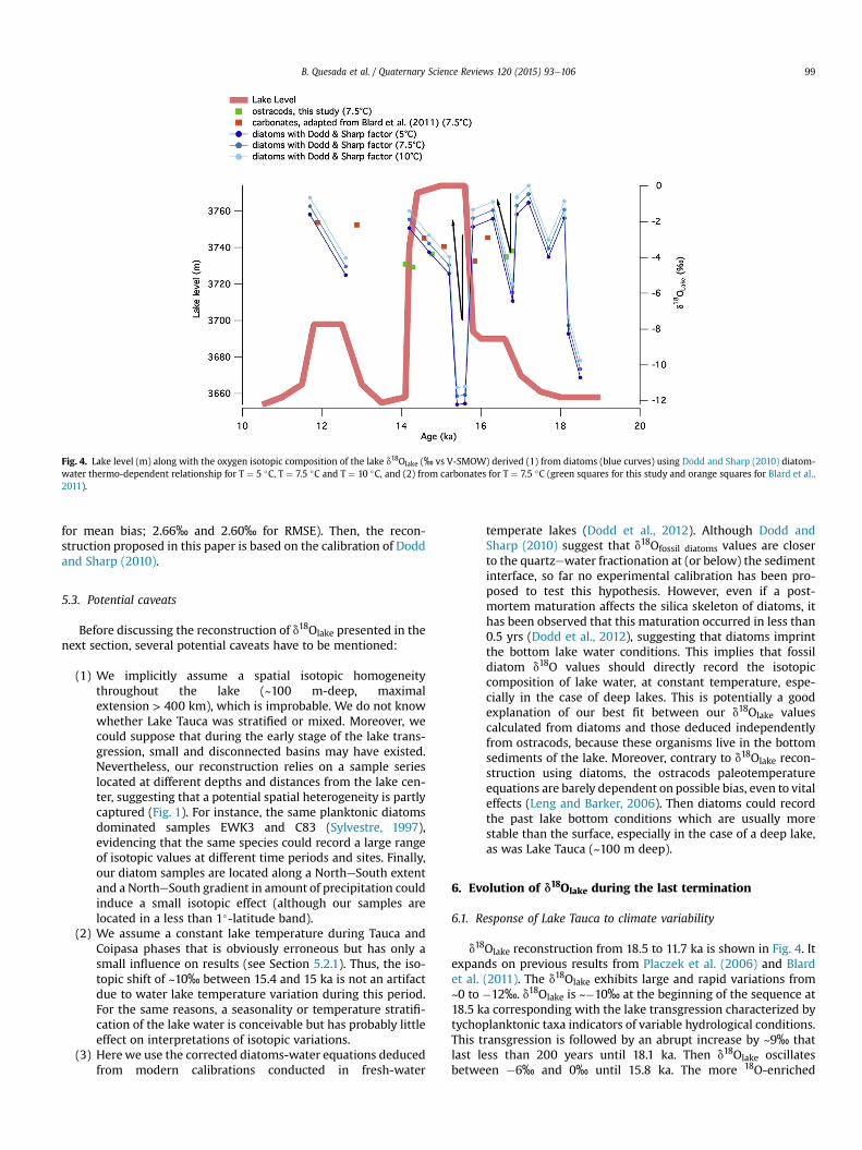
Fig. 4. Lake level (m) along with the oxygen isotopic composition of the lake d18Olake (‰ vs V-SMOW) derived (1) from diatoms (blue curves) using Dodd and Sharp (2010) diatom-water thermo-dependent relationship for T ¼ 5 �C, T ¼ 7.5 �C and T ¼ 10 �C, and (2) from carbonates for T ¼ 7.5 �C (green squares for this study and orange squares for Blard et al.,2011).

B. Quesada et al. / Quaternary Science Reviews 120 (2015) 93e106 99

for mean bias; 2.66‰ and 2.60‰ for RMSE). Then, the recon-struction proposed in this paper is based on the calibration of Doddand Sharp (2010).

5.3. Potential caveats

Before discussing the reconstruction of d18Olake presented in thenext section, several potential caveats have to be mentioned:

(1) We implicitly assume a spatial isotopic homogeneitythroughout the lake (~100 m-deep, maximalextension > 400 km), which is improbable. We do not knowwhether Lake Tauca was stratified or mixed. Moreover, wecould suppose that during the early stage of the lake trans-gression, small and disconnected basins may have existed.Nevertheless, our reconstruction relies on a sample serieslocated at different depths and distances from the lake cen-ter, suggesting that a potential spatial heterogeneity is partlycaptured (Fig. 1). For instance, the same planktonic diatomsdominated samples EWK3 and C83 (Sylvestre, 1997),evidencing that the same species could record a large rangeof isotopic values at different time periods and sites. Finally,our diatom samples are located along a NortheSouth extentand a NortheSouth gradient in amount of precipitation couldinduce a small isotopic effect (although our samples arelocated in a less than 1�-latitude band).

(2) We assume a constant lake temperature during Tauca andCoipasa phases that is obviously erroneous but has only asmall influence on results (see Section 5.2.1). Thus, the iso-topic shift of ~10‰ between 15.4 and 15 ka is not an artifactdue to water lake temperature variation during this period.For the same reasons, a seasonality or temperature stratifi-cation of the lake water is conceivable but has probably littleeffect on interpretations of isotopic variations.

(3) Herewe use the corrected diatoms-water equations deducedfrom modern calibrations conducted in fresh-water

temperate lakes (Dodd et al., 2012). Although Dodd andSharp (2010) suggest that d18Ofossil diatoms values are closerto the quartzewater fractionation at (or below) the sedimentinterface, so far no experimental calibration has been pro-posed to test this hypothesis. However, even if a post-mortem maturation affects the silica skeleton of diatoms, ithas been observed that this maturation occurred in less than0.5 yrs (Dodd et al., 2012), suggesting that diatoms imprintthe bottom lake water conditions. This implies that fossildiatom d18O values should directly record the isotopiccomposition of lake water, at constant temperature, espe-cially in the case of deep lakes. This is potentially a goodexplanation of our best fit between our d18Olake valuescalculated from diatoms and those deduced independentlyfrom ostracods, because these organisms live in the bottomsediments of the lake. Moreover, contrary to d18Olake recon-struction using diatoms, the ostracods paleotemperatureequations are barely dependent on possible bias, even to vitaleffects (Leng and Barker, 2006). Then diatoms could recordthe past lake bottom conditions which are usually morestable than the surface, especially in the case of a deep lake,as was Lake Tauca (~100 m deep).

6. Evolution of d18Olake during the last termination

6.1. Response of Lake Tauca to climate variability

d18Olake reconstruction from 18.5 to 11.7 ka is shown in Fig. 4. Itexpands on previous results from Placzek et al. (2006) and Blardet al. (2011). The d18Olake exhibits large and rapid variations from~0 to �12‰. d18Olake is ~�10‰ at the beginning of the sequence at18.5 ka corresponding with the lake transgression characterized bytychoplanktonic taxa indicators of variable hydrological conditions.This transgression is followed by an abrupt increase by ~9‰ thatlast less than 200 years until 18.1 ka. Then d18Olake oscillatesbetween �6‰ and 0‰ until 15.8 ka. The more 18O-enriched

B. Quesada et al. / Quaternary Science Reviews 120 (2015) 93e106100

composition (ca 0‰) during this phase is recorded during the initialrise of the lake level at around 17.2 ka. At 16.9 ka, a d18Olakedepletion of 5‰ is followed by a d18Olake enrichment of 4‰ until15.8 ka. Then, an exceptional d18Olake drop of 10‰ occurs probablyin less than 200 years (see Table 2 column c, for EWK6 and EWK7samples) during the main lacustrine transgression around 15.8 ka.This abrupt drop is followed by a sudden increase of ~7‰ from15.4 ka to 14.8 ka (see black arrows on Fig. 4). This particular 2-stepd18Olake variation (d18Olake depletion followed by a d18Olake re-enrichment) is the so-called “remarkable isotopic feature” studiedin the following sections. Note also that the two abrupt isotopicdrops at 16.9 ka and 15.8 ka are concomitant with the two suc-cessive fillings of the lake during its transgression.

The abrupt d18Olake decrease during lake filling can easily beexplained by a regional increase in precipitation (Dansgaard, 1964;Ramirez et al., 2003; Vimeux et al., 2005; Risi et al., 2010). More-over, this feature appears particularly robust as diatom samplesexhibiting this d18Olake drop are of high purity (>99% of silica e seeTable 1 for EWK6 and EWK7 samples). However, d18Olake increasesmeasured during stable lake level phases are more surprising ob-servations. This d18Olake re-enrichment has been also recorded atsimilar timescales in pluvial paleo-lake Bonneville during fillingphases (see Figure 7 of McGee et al., 2012). One explanation isrelated to the lake evaporation and the associated isotopic frac-tionation leading to an enrichment of the isotopic composition ofthe lake. According to climate archives in the Andes such as icecores (at Illimani and Huascaran, Ramirez et al., 2003; Thompsonet al., 1995) or speleothems (Kanner et al., 2012; Mosblech et al.,2012), the isotopic composition of precipitation in this region wasdepleted during the last termination compared to present-dayvalues (estimated around a �14‰ annual average on the Alti-plano (IAEA, 2004)). Thus, according to our reconstruction, the lakemay have undergone strong evaporation over most of the studiedperiod (Fig. 4).

In order to test the potential impact of evaporation on d18Olake, asimple hydro-isotopic model is developed in the next section. Thismodel is applied to the Tauca phase onset (around 15.8 ka) forwhich a number of parameters have been constrained in previousstudies (Thompson et al., 1998; Condom, 2002; Coudrain et al.,2002; Condom et al., 2004; Vimeux et al., 2005; Blard et al.,2009; this study).

6.2. Impact of lake evaporation on d18Olake during the Tauca phase?

6.2.1. The hydro-isotopic modelAn iterative (annual step) hydro-isotopic model is developed

accounting for the Tauca watershed system. It does not take intoaccount external inputs such as groundwater and runoff (see Sec-tion 6.3 for further discussions). The model is based on the Taucawatershed hydrological (equation (1)) and isotopic (equation (2))balances as:

dVLake

dt¼ ðPðtÞ � EðtÞÞ$S (1)

dðdLake$VLakeÞdt

¼ �dp$PðtÞ � de$EðtÞ

�$S (2)

where S is the total surface of the Tauca watershed (lake plus soil):138.875 km2 (Blard et al., 2011), P(t) and E(t) are the evolution ofprecipitation and the total evaporation over the Tauca watershedrespectively, dVLake/dt is the volume variation of the lake as definedby Condom et al. (2004) as a function of the lake level, dlake(t) is theisotopic composition of the lake, dp(t) and de(t) are the isotopiccomposition of incoming precipitation and evaporative flux

respectively. The latter is calculated using the (Craig and Gordon,1965) equation:

deðtÞ ¼dlakeðtÞ � hðtÞ$datmðtÞ þ εvelðtÞ þ εdiff ðtÞ

1� hðtÞ (3)

where h(t) is the relative humidity normalized to temperature atthe lake water surface, datm(t) is the isotopic composition of theatmosphere above the lake (which is supposed to be in isotopicequilibrium with dp(t) in our study); εvel (<0) and εdiff (<0) are theequilibrium and diffusion (or kinetic) fractionation parametersdefined as:

εvel ¼ avel � 1 ¼ 1alev

� 1 (4)

with alev ¼ exp�1:137T2

$1000� 0:4156T

� 0:0020667�

¼ dl þ 1000dv þ 1000

(5)

where alev is the oxygen isotopic equilibrium fractionation factorbetween liquid and vapor for oxygen 18 (>1) (Majoube, 1971) (T in�K). We consider atmospheric temperature constant at 2.5 �C (seeSection 5.2.1).

εdiff ¼ ð1� hðtÞÞ$�1�

�DDi

�n�(6)

where D and Di are the molecular diffusivities of H216O and H2

18Orespectively with a ratio of D/Di ¼ 1/0.9723 (Merlivat, 1978), n is aturbulence parameter linked to the surface roughness which isestimated to be 0.5 for mean turbulent flow for a large lake(Gonfiantini, 1986).

At each step, lake isotopic variations are computed and dlake(t) isdeduced from Equation (2) as:

dlakeðtÞ ¼ dlakeðt � 1Þ þ�ddlakedt

�t�1

$Dt (7)

Finally, we can write dlake(t) from equations (1)e(3) and (7) as:

ddlakedt

þ dlaket

¼ Aþ Bt

(8)

with t ¼ VlakeðtÞdVlakedt þ EðtÞ

1�hðtÞ; A ¼ dpðtÞ$PðtÞ$S

dVlakedt þ EðtÞ

1�hðtÞ;

B ¼ hðtÞ$datmðtÞ � εvel � εdiff ðtÞdVlakedt þ EðtÞ

1�hðtÞ$

EðtÞ1� hðtÞ

During the stable phase (dVlake/dt ¼ 0, dSlake/dt ¼ 0), the secondterm (A þ B)/t of equation (8) is constant and dlake takes an expo-nential shape with a time constant t ¼ ((1 � h)Vlake/E). The dlakecould be considered invariant after about 5t.

Our model is applied during the Tauca phase onset (t0 ¼ 0 year,around 15.8 ka) until the lake level stabilization at tTauca¼ 100 years(dVlake/dt and dSlake/dt ¼ 0). As a first exploration, we use a stabi-lization time of 100 years which is the lowest estimate given byCondom(2002), and less than the agedifference betweenEWK6andEWK7 samples (~200 years) which defines the abrupt d18Olake fall.h(t) is supposed to increase from 0.4 to 0.6 during the lake filling. Alinear increase in lake altitude from 3650 to 3770 m is defined. P(t)increases linearly from P0 ¼ 400 mm/year (probably higher thanpresent-day value (300 mm/year) due to wetter conditions) to

B. Quesada et al. / Quaternary Science Reviews 120 (2015) 93e106 101

PTauca¼ 600mm/year as suggested by Blard et al. (2011).We deducethe dp(t) variation from P(t) variation according to the isotopic-precipitation gradient of �0.02‰/(mm/year) (Rozanski et al., 1993)and considering that dp at t0 is �20‰ (see section 7).

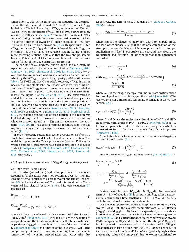
6.2.2. Model resultsModel results are shown in Fig. 5 as a function of time. We

clearly see that our model is able to reproduce the 2-step d18Olakevariation (so-called “remarkable isotopic feature”) exhibited in ourobservations:

(1) as the lake level increases, the simulated d18Olake decreases,in line with the expected influence of precipitation increaseas aforementioned. Moreover, quantitatively, the d18Olakedrop is ~17‰ which is consistent with our observations at15.8 ka, albeit overestimated (~10‰ in data).

(2) at tTauca, a rebound of d18Olake is simulated. The temporalconstant t is of ~25 years, leading to a constant d18Olake after100 years, consistent with the timing of the abrupt increasesobserved in our reconstruction at ~15.4 ka. This isotopic lakere-enrichment is also simulated by our model (~4‰) albeitslightly lower than our observations (~7‰).

To test the validity of the model results, we performed sensi-tivity tests with tunable h(t) and P(t) evolutions, dp at t0 and tTauca(Table 4). The most sensitive parameter is tTauca: the more tTaucadecreases, themore d18Olake is enriched, up to 16‰when tTauca¼ 50years.

Fig. 5. Hydro-isotopic model results with the parameters mentioned in Table 4 and in Sectioin ‰; Surface (km2) and Volume (km3) of the lake; Precipitation P(t) and Evaporation E(t)

An important assumption in our model deals with the isotopicequilibrium between datm(t) and dp(t). To check the validity of themodel results, we reduce the datm(t) � dp(t) difference by enrichingdatm(t) (this mimics a possible realistic change of datm(t) when lakeevaporates). This leads to a more pronounced enrichment ind18Olake, more than doubling when datm (t) tends to dp(t).

Thus, we are able to reproduce the d18Olake variations duringLake Tauca filling phase and the following stable phase, consideringonly the hydrological and isotopic balances of the Tauca watershedand the associated isotopic fractionation. The main reason for thisremarkable isotopic feature lies in the competition betweenevaporation and precipitation: while precipitation increases, thereduction, albeit the inhibition, of evaporation before lake stabili-zation leads to the depletion of the lake's isotopic composition.When precipitation becomes constant, evaporation is no longerrestricted and tends to enrich the lake's isotopic composition. Ourmodel is able to reproduce the d18Olake amplitude increase at15.4 ka only when Tauca filling time is reduced to around 50 years,compared to previous estimates (see Table 4). The next sectionexploreswhether a fraction of the d18Olake enrichment could be alsoexplained by the Titicaca inputs.

6.3. Potential role of the Desaguadero River in lake isotopic balanceduring the Tauca episode

Hydrologic sources from Lake Titicaca during the Tauca episodeare controversial: among related studies, some suggest a flow rateof the Desaguadero River between 3 and 30 times higher than its

n 6.2.1. From top to bottom: d18O of the lake, d18Olake (blue) and the precipitation (pink)in the Tauca watershed (km3/year).

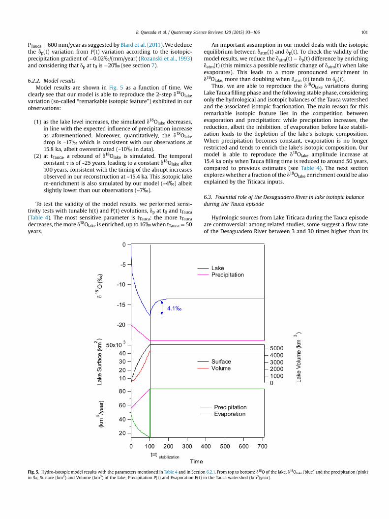
Table 4Sensitivity tests performed on themain parameters of the simple hydro-isotopical model. Each parameter (a, b) is modified around its default value (c) by ~±20% (d) to evaluatethe d18Olake increase during stable level phase (e). Only one parameter is modified for each sensitivity test. d18Olake increase is ~4.1‰ with the aforementioned defaultparameterization. tTauca is 100 years with tested range coherent with (Condom, 2002). Relative humidity at T ¼ 0 is fixed at 0.4 (and increases to 0.6 at tTauca) but has only aminor influence on d18Olake.

Parametera

Characterizationb

Default valuec

Range of changed

Literature constraintse

18O increase duringstable level phasef

hTauca Humidity after tTauca 0.6 [0.4; 0.8] e [0.2; 8.4] ‰P(0) Precipitation before Tauca phase 400 mm/yr [300; 500] e [4.0; 4.3] ‰PTauca Precipitation after Tauca phase 600 mm/yr [400; 800] (Blard et al., 2009) [1.8; 8.7] ‰dP0

18O composition before Tauca phase �20‰ [�15; �25] (Thompson et al., 1998) 4.1‰aP Local amount effect �0.02‰/mm.yr [�0.06; 0] (Vimeux et al., 2005) [1.8; 5.2] ‰STOT Tauca catchment area 138,875 km2 [100,000; 170,000] (Blard et al., 2009); (Condom, 2002) [2.8; 7.6] ‰tTauca Time of Tauca filling phase 100 years [50; 300] This study; (Condom, 2002) [0.7; 15.7] ‰

B. Quesada et al. / Quaternary Science Reviews 120 (2015) 93e106102

actual flow (Cross et al., 2001; Coudrain et al., 2002; Grove et al.,2003) although a recent study suggests minimal input from LakeTiticaca (Placzek et al., 2011). Moreover, the available water amountprovided by surrounding glaciers would have been insufficient tosubstantially fill Lake Tauca (Blodgett et al., 1997; Condom, 2002)since their maximal extension was reached during the Tauca phase(Blard et al., 2009; Zech et al., 2011). Thus, the inputs from LakeTiticaca and from surrounding glaciers for which no isotopic con-straints are known were not taken into account in the first step ofour model. We tend nonetheless in this section to explore thepossible impact of overflowing via the Desaguadero River. Wequestion the role of the Desaguadero River in enriching the pale-olake Tauca and in increasing the simulated isotopic re-enrichment(i.e “extra re-enrichment”) during the Tauca stable phase. For this,we add a term for input from Desaguadero Q(t) to our model withits corresponding isotopic composition d18OQ, without changingthe total input budget I(t) (600 mm/year, see Table 4):

dVLake

dt¼ ðIðtÞ � EðtÞÞ$S (9)

dðdLake$VLakeÞdt

¼ �dp$PðtÞ þ dQ$QðtÞ � de$EðtÞ

�$S (10)

IðtÞ ¼ PðtÞ þ QðtÞ (11)

Two extreme scenarios of Desaguadero flow evolution duringthe Tauca phase are considered:

(1) An “Abrupt scenario”: Q(t) is negligible versus precipitationinput, P(t), during Tauca filling phase (t < tTauca) but equal toQTauca (km3/yr) when t ¼ tTauca.

(2) A “Progressive scenario”: Q(t) linearly increases from t0 totTauca from 0 to QTauca (km3/yr) then is equal to QTauca aftertTauca.

We consider (1) a range of Desaguadero contribution varyingfrom 0% to 70% of the total input budget e which roughly corre-sponds to interval given by above-cited literature e and (2) aconstant Desaguadero isotopic value during the stabilization phase.We test d18OQ values from �20 to 0 ‰.

While scenario 2 exhibits an extra re-enrichment varying from amaximum value of 0‰ (with QTauca ¼ 0%$ITauca) to minimum oneof �1.9‰ (with QTauca ¼ 70%$ITauca and d18OQ ¼ 0‰), scenario 1displays an extra re-enrichment from 0‰ (with QTauca ¼ 0%$ITauca)to þ6.7‰ (with QTauca ¼ 70%$ITauca and d18OQ ¼ 0‰).

In conclusion, the progressive scenario is unable to explain anextra re-enrichment: it contributes to slightly lower the lake re-enrichment. On the contrary, with the abrupt scenario, the

Desaguadero River could have substantially contributed to theisotopic lake re-increase from 0 to 6.7‰. In this case, the Desa-guadero input could complete the enrichment simulated by oursimple hydro-isotopic model (with tstabilization ¼ 100 years) andthen explain the d18Olake 7‰-re-enrichment in our observations at15.4 ka. Thus, in this case and assuming highest Titicaca outflowestimates, the Desaguadero input could complete the enrichmentsimulated by our simple hydro-isotopic model (withtstabilization ¼ 100 years) and then explain the d18Olake 7‰-re-enrichment in our observations at 15.4 ka. In all the other cases,Desaguadero impact on Tauca isotopic balance is almost negligible.

7. Role of Lake Tauca on the isotopic composition ofprecipitation on Andean summits: case of the Sajama

In this section, we explore to what extent the disappearance ofLake Tauca played a role in the isotopic records from Sajama.Indeed, several studies pointed out the intense convection (e.g.Blodgett et al., 1997) and the water recycling (e.g. Blard et al., 2009)above the lake during Tauca phase that could have providedmoisture, eventually further advected towards Sajama summit.These processes are common among pluvial lakes and are likely tocontribute substantially to maintain these lakes (Hostetler et al.,1994; Laabs et al., 2009; Mcgee et al., 2012).

Based on the new chronological constraints on Lake Taucaregression (Blard et al., 2011) and accounting for dating un-certainties on ice cores, the abrupt d18O isotopic excursion of þ7‰recorded in the Sajama ice core between 15 and 14 ka now appearssynchronous with the regression of Lake Tauca (see Fig. 2). Wequestion the potential contribution of the lake evaporation when itdisappears as a moisture source for precipitation at Sajama. Weexamine whether the enrichment at Sajama could be explained bymoisture supply from paleolake Tauca.

Our discussion will only be based on the isotopic balance. Weassume that the signal of the isotopic composition of incomingprecipitation on the Altiplano at ~14 ka is d18Op ¼ �20‰ (contraryto d18Op ¼ �14‰ at Sajama) (see Fig. 2). This estimate correspondsto a d18Op depletion of about 4‰ compared with the modern d18Op

at Illimani. The latter can be estimated by the average value of d18Oin Illimani ice core over the last 100 years (Vimeux, 2009). Thisdepletion of 4‰ between 14 ka and present-day is of the sameorder than the onewe observe at Huascaran (this is also the value ofd18O in Illimani ice core at ~14 ka if we consider that the dating fromRamirez et al., 2003 is correct). Assuming condensation at isotopicequilibrium at T ¼ 2.5 �C (estimated atmospheric mean tempera-ture, see section 5.2.1), the isotopic composition of water vaporfrom which precipitation forms is �31‰ (versus �25‰ at Sajama)and will be considered as the isotopic composition of the back-ground atmosphere.

B. Quesada et al. / Quaternary Science Reviews 120 (2015) 93e106 103

We first consider an extreme situation (although unrealistic)corresponding to a complete and instantaneous lake evaporation.In this case, no isotopic fractionation occurs between the lakewaterand the atmosphere and, considering that d18Olake is about 5‰ atthe lake highest level (Fig. 4), the water vapor input in the atmo-sphere would have an isotopic composition of d18Ov ¼ �5‰.Consequently, based solely on the isotopic balance, the relativecontribution of advected vapor versus vapor originating from thelake (x) to precipitation at Sajama can be estimatedas �25‰ ¼ (1 � x)(�31‰) þ (x)(�5‰). Thus, the lake contributionto Sajama precipitation versus advected water vapor would be 23%.It is worth noting that this calculation is sensitive to d18Oatm andvaries of about þ3%/per mil when d18Oatm varies between �25and �35‰.

We now consider a progressive evaporation of Lake Tauca. Weuse the evaporative model from Gonfiantini (1986) derived fromCraig and Gordon (1965). The evolution of the lake's isotopiccomposition, according to the fraction of remaining water in thelake (f, the lake evaporates as f tends to 0), is given by:

ddlaked ln f

¼h$ðdlake � datmÞ � ðdlake þ 1Þ$

�� εvel�εdiff

�1� h� εdiff

(12)

As an initial exploration, we consider constant conditions forlake evaporation (h ¼ 0.6, d18Oatm ¼ �31‰, T ¼ 2.5 �C). A simpleintegration of equation (12) leads to:

dlakeðf Þ ¼�d0 �

AB

�$f B þ A

B(13)

where:A ¼ h$datm�εdiff�εvel

1�h�εdiff; B ¼ hþεdiffþεvel

1�h�εdiff; and the initial d18Olake is

d0¼�5‰.Using equation (13), we can deduce the evolution of d18Olake as a

function of f, as well as the evolution of the isotopic composition ofevaporated water (using equation (3)). In that case, de variesfrom�8.75‰ (f ¼ 1) to�3.32‰ (f ¼ 0) and the lake contribution toSajama precipitation decreases from 27 (f ¼ 1) to 22% (f ¼ 0). It isworth noting that this result is highly sensitive to h and to a lesserextent to d18Oatm. We run the model with varying h and d18Oatm.Simulations are shown on Fig. 6a and b. Considering all simulations,the extra enrichment of 5‰ at Sajama can be explained with awater vapor input from lake evaporation varying from 10 to 60%(see lake contribution on Fig. 6a and b when f ¼ 0).

We nowconsider varying conditions during lake evaporation forh and d18Oatm. Indeed, the continuous evaporation of the lakemodifies those two parameters as the evaporation occurs. Wenumerically solve equation (12) by successive iterations (we keep aconstant temperature of 2.5 �C and the initial d18Oatm is of �31‰.).We consider that h decreases from 0.6 to 0.4. In equation (3),d18Oatm is the isotopic composition of the atmosphere in contactwith the lake during the lake transgression. We account for theinfluence of the lake evaporation on d18Oatm at each iteration (j) sothat d18Oatm at the step (j) is calculated as a mixed value of de andd18Oatm at the previous step (j � 1): d18Oatm(j) ¼ n*de(j � 1) þ(1 � n)d18Oatm(j � 1). We decide that n is related to f as n¼ (1 � xf)*f: we account here for the fact that when f ¼ 1 there is no lakecontribution and when f ¼ 0 there is a maximal mixing between deand d18Oatm which is represented by xf. Fig. 6c shows the lakecontribution for different xf. We clearly see that the isotopicexcursion at Sajama can be explained by a significant water vaporinput from the lake evaporation at the beginning of lake disap-pearance (from almost 50%) which tends to decrease to 0 when thelake disappears as expected.

To conclude, we find in each simulation that around 70% of theabrupt d18O isotopic excursion of þ7‰ recorded in the Sajama icecore between 15 and 14 ka can be explained by the disappearanceof Lake Tauca, with a lake contribution varying from a few percentto 60%.

As aforementioned, our calculations are only based on the isotopicbalance and do not account for the water availability betweenadvected moisture and lake evaporation. We try here to estimatewhether these contributions are realistic. A lake volume of 4600 km3

corresponds to PTauca¼ 83.3 km3/year (0.6m/year*138,875 km2) (seeFig. 5). The full disappearance of the lake in 300 years gives a lakewater volume availability of 15.3 km3/year (4600 km3/300 years).Wenow have to estimate the reduction of PTauca during lake disappear-ance. For a reduction of 2 (resp. 3) the evaporated moisture versusadvected precipitation in volume, and thus the maximum lakecontribution to Sajama precipitation, is 37% (¼ 15.3/(83.3/2)) (resp.55% ¼ 15.3/(83.3/3)). Considering the range of PTauca given in Table 3anda reductionofPTauca that canattain a factor3,weestimate that themaximum lake contribution in terms of water volume versus advec-ted water could vary between 27 and 82%, which is higher than ouraforementioned estimates. Consequently, we estimate that thewatervolume evaporated above the lake can be enough to substantiallycontribute to the isotopic excursion in the Sajama ice core signal.

8. Conclusion

TheBolivianAltiplano is a unique case for exploring the impact oflakes on surrounding continental climate archives due to theproximity of paleolakes and ice caps. In this paper, we propose forthe first time a quantitative reconstruction of the oxygen 18 isotopicvariations (d18O) of the Bolivian Altiplano paleolakes from 18.5 to11.7 ka based on the isotopic composition of fossil diatoms and os-tracods. Considering some assumptions (constant lake temperature,choice of the diatoms-water calibration, spatial homogeneity of thelake isotopic composition), a robust feature is evidenced in theevolution of d18Olake. An abrupt decrease of d18Olake during lakefillings is immediately followed by an increase of d18Olake duringstable lake level phases. The highest variation occurs at 15.8 kawitha d18Olake decrease of about 10‰ concomitant with the Lake Taucatransgression, followed by a d18Olake increase of similar amplitudefour centuries later, in pace with the lake highstand stabilization.

With a simple hydro-isotopic modeling approach, it is possibleto satisfactorily reproduce the 2-step (“decreaseeincrease”)d18Olake variation exhibited in our data. Moreover, this study revealsthat the renewed increases of d18Olake after filling phases can bepartly explained by the prior reduction of evaporative flux due tohigh rainfall and a consecutive re-equilibration of the isotopicfluxes in lake steady-state. This explanation assumes a rapid (lessthan a few centuries) set-up of high rainfall regime. Our modelintegrates consistent and available constraints on humidity, pre-cipitation, isotopic compositions and geomorphological parametersfrom the literature and our sensitivity tests show its robustness.However, it remains a simple modeling approach that does not takeinto account, for example, the seasonality of precipitation, runoffand groundwater, and assumes linear variations of main variables.

The d18Olake reconstruction enables us to explore whether the‘paleolakes’ presence have influenced the isotopic composition ofprecipitation deposited at Sajama. We conclude that the total orpartial evaporation of the lake during the Tauca phase regressioncould explain the distinct isotopic excursion at Sajama. We showthat a contribution of the lake evaporation to precipitation atSajama from a few percent to 60% during the lake disappearance issufficient to explain the 5‰ extra enrichment and is consistentwith available water volume. Consequently, perturbation of localhydrological cycles by lacustrine basins could, at certain periods,

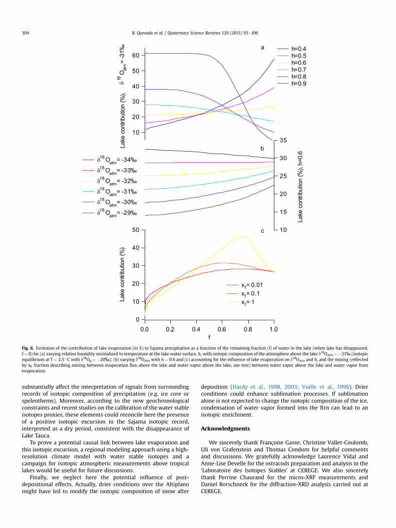
Fig. 6. Evolution of the contribution of lake evaporation (in %) to Sajama precipitation as a function of the remaining fraction (f) of water in the lake (when lake has disappeared,f ¼ 0) for (a) varying relative humidity normalized to temperature at the lake water surface, h, with isotopic composition of the atmosphere above the lake d18Oatm ¼ �31‰ (isotopicequilibrium at T ¼ 2.5 �C with d18Op ¼ �20‰); (b) varying d18Oatm with h ¼ 0.6 and (c) accounting for the influence of lake evaporation on d18Oatm and h, and the mixing (reflectedby xf, fraction describing mixing between evaporation flux above the lake and water vapor above the lake, see text) between water vapor above the lake and water vapor fromevaporation.

B. Quesada et al. / Quaternary Science Reviews 120 (2015) 93e106104

substantially affect the interpretation of signals from surroundingrecords of isotopic composition of precipitation (e.g. ice core orspeleothems). Moreover, according to the new geochronologicalconstraints and recent studies on the calibration of the water stableisotopes proxies, these elements could reconcile here the presenceof a positive isotopic excursion in the Sajama isotopic record,interpreted as a dry period, consistent with the disappearance ofLake Tauca.

To prove a potential causal link between lake evaporation andthis isotopic excursion, a regional modeling approach using a high-resolution climate model with water stable isotopes and acampaign for isotopic atmospheric measurements above tropicallakes would be useful for future discussions.

Finally, we neglect here the potential influence of post-depositional effects. Actually, drier conditions over the Altiplanomight have led to modify the isotopic composition of snow after

deposition (Hardy et al., 1998, 2003; Vuille et al., 1998). Drierconditions could enhance sublimation processes. If sublimationalone is not expected to change the isotopic composition of the ice,condensation of water vapor formed into the firn can lead to anisotopic enrichment.

Acknowledgments

We sincerely thank Françoise Gasse, Christine Vallet-Coulomb,Uli von Grafenstein and Thomas Condom for helpful commentsand discussions. We gratefully acknowledge Laurence Vidal andAnne-Lise Develle for the ostracods preparation and analysis in the‘Laboratoire des Isotopes Stables’ at CEREGE. We also sincerelythank Perrine Chaurand for the micro-XRF measurements andDaniel Borschneck for the diffraction-XRD analysis carried out atCEREGE.

B. Quesada et al. / Quaternary Science Reviews 120 (2015) 93e106 105

This work was funded by IRD (Institut de Recherche pour leD�eveloppement).

References

Alexandre, A., Basile-Doelsch, I., Sonzogni, C., Sylvestre, F., Parron, C., Meunier, J.D.,Colin, F., 2006. Oxygen isotope analyses of fine silica grains using laser-extraction technique: comparison with oxygen isotope data obtained fromion microprobe analyses and application to quartzite and silcrete cementinvestigation. Geochim. Cosmochim. Acta 70, 2827e2835.

Alexandre, A., Crespin, J., Sylvestre, F., Sonzogni, C., Hilbert, D.W., 2012. The oxygenisotopic composition of phytolith assemblages from tropical rainforest soil tops(Queensland, Australia): validation of a new paleoenvironmental tool. Clim.Past 8, 307e324.

Baker, P.A., Rigsby, C.A., Seltzer, G.O., Fritz, S.C., Lowenstein, T.K., Bacher, N.P.,Veliz, C., 2001a. Tropical climate changes at millennial and orbital timescales onthe Bolivian Altiplano. Nature 409, 698e701.

Baker, P.A., Seltzer, G.O., Fritz, S.C., Dunbar, R.B., Grove, M.J., 2001b. The history ofSouth American tropical precipitation for the past 25,000 years. Science 291,640e643.

Blard, P.-H., Lav�e, J., Farley, K.A., Fornari, M., Jim�enez, N., Ramirez, V., 2009. Late localglacial maximum in the Central Altiplano triggered by cold and locally-wetconditions during the paleolake Tauca episode (17e15ka, Heinrich 1). Quat.Sci. Rev. 28, 3414e3427.

Blard, P.-H., Sylvestre, F., Tripati, A.K., Claude, C., Causse, C., Coudrain, A., Condom, T.,Seidel, J.-L., Vimeux, F., Moreau, C., Dumoulin, J.-P., Lav�e, J., 2011. Lake high-stands on the Altiplano (Tropical Andes) contemporaneous with Heinrich 1 andthe Younger Dryas: new insights from 14C, UeTh dating and d18O of carbonates.Quat. Sci. Rev. 30, 3973e3989.

Blodgett, T.A., Isacks, B.L., Lenters, J.D., 1997. Constraints on the origin of paleolakeexpansions in the Central Andes. Earth Interact. 1, 1e28.

Brandriss, M.E., O'Neil, J.R., Edlund, M.B., Stoermer, E.F., 1998. Oxygen isotopefractionation between diatomaceous silica and water. Geochim. Cosmochim.Acta. 62, 1119e1125.

Chapligin, B., Leng, M., Webb, E., Alexandre, A., Dodd, J., Faure, K., Ijiri, A., Lücke, A.,Shemesh, A., Abelmann, A., Herzschuh, U., Longstaffe, F., Meyer, H., Moschen, R.,Okazaki, Y., Rees, N.H., Sharp, Z., Sloane, H.J., Sonzogni, C., Swann, G.,Sylvestre, F., Tyler, J., Yam, R., 2011. Interlaboratory comparison of oxygen iso-topes from biogenic silica. Geochem. Cosmochim. Acta. http://dx.doi.org/10.1016/j.gca.2011.08.011.

Condom, T.H., 2002. Dynamiques d'extension lacustre et glaciaire associ�ees auxmodifications du climat dans les Andes Centrales (Ph.D. thesis). University ofParis VI-Pierre et Marie Curie, Paris, France.

Condom, T., Coudrain, A., Dezetter, A., Brunstein, D., Delclaux, F., Sicart, J.E., 2004.Transient modelling of lacustrine regressions: two case studies from the An-dean Altiplano. Hydrol. Process. 18, 2395e2408.

Coudrain, A., Loubet, M., Condom, T., Talbi, A., Ribstein, P., Pouyaud, B.,Quintanilla, J., Dieulin, C., Dupr�e, B., 2002. Donn�ees isotopiques (87Sr/86Sr) etchangements hydrologiques depuis 15 000 ans sur l'Altiplano andin. Hydrol.Sci. J. 47, 293e306.

Craig, H., Gordon, L.I., 1965. Deuterium and oxygen 18 variations in the ocean andmarine atmosphere. In: Proc. Stable Isotopes in Oceanographic Studies andPaleotemperatures. E.Tongiogi, Pisa (Italy), pp. 9e130.

Crespin, J., Alexandre, A., Sylvestre, F., Sonzogni, C., Paill�es, C., Garreta, V., 2008. IRlaser extraction technique applied to oxygen isotope analysis of small biogenicsilica samples. Anal. Chem. 80, 2372e2378.

Crespin, J., Sylvestre, F., Alexandre, A., Sonzogni, C., Paill�es, C., Perga, M.-E., 2010. Re-examination of the temperature-dependent relationship between d18Odiatomsand d18Olake water and implications for paleoclimate inferences. J. Paleolimnol.44, 547e557.

Cross, S.L., Baker, P.A., Seltzer, G.O., Fritz, S.C., Dunbar, R.B., 2001. Late Quaternaryclimate and hydrology of tropical South America inferred from an isotopic andchemical model of Lake Titicaca Bolivia and Peru. Quat. Res. 56, 1e9.

Dansgaard, W., 1964. Stables isotopes in precipitation. Tellus 16, 436e447.Dodd, J.P., Sharp, Z.D., 2010. A laser fluorination method for oxygen isotope analysis

of biogenic silica and a new oxygen isotope calibration of modern diatoms infreshwater environments. Geochim. Cosmochim. Acta 74, 1381e1390.

Dodd, J.P., Sharp, Z.D., Fawcett, P.J., Brearley, A.J., McCubbin, F.M., 2012. Rapid post-mortem maturation of diatom silica oxygen isotope values. Geochem. Geophys.Geosyst. 13 http://dx.doi.org/10.1029/2011GC004019.

Friedman, I., O'Neil, J.R., 1977. Compilation of stable isotope fractionations factors ofgeochemical interest. In: Friedman, I., O'Neil, J.R. (Eds.), Data of Geochemistry.U.S. Geol. Surv., Washington, DC, pp. KK1eKK12.

Garreaud, R.D., Vuille, M., Clement, A.C., 2003. The climate of the Altiplano:observed current conditions and mechanisms of past changes. Palaeogeogr.Palaeoclim. Palaeoecol. 194, 5e22.

Garreaud, Aceituno, 2001. Interannual rainfall variability over the South AmericanAltiplano. J. Clim. 14, 2779e2789.

Gonfiantini, R., 1986. Environmental isotopes in lake studies. In: Fritz, P., Fontes, J.Ch(Eds.), Handbook of Environmental Isotope Geochemistry, vol. 3. Elsevier, NewYork, pp. 113e168.

von Grafenstein, U., Erlernkeuser, H., Trimborn, P., 1999. Oxygen and carbon iso-topes in modern fresh-water ostracod valves: assessing vital offsets and

autecological effects of interest for palaeoclimate studies. Palaeogeogr. Palae-oclim. Palaeoecol. 148, 133e152.

Grove, M.J., Baker, P.A., Cross, S.L., Rigsby, C.A., Seltzer, G.O., 2003. Application ofstrontium isotopes to understanding the hydrology and paleohydrology of theAltiplano, Bolivia-Peru. Palaeogeogr. Palaeoclim. Palaeoecol. 194, 281e297.

Hardy, D.R., Vuille, M., Braun, C., Keimig, F., Bradley, R.S., 1998. Annual and dailymeteorological cycles at high altitude on a tropical mountain. Bull. Am. Mete-orol. Soc. 79, 1899e1913.

Hardy, D.R., Vuille, M., Bradley, R.S., 2003. Variability of snow accumulation andisotopic composition on Nevado Sajama, Bolivia. J. Geophys. Res. 108 (D22),4693. http://dx.doi.org/10.1029/2003JD003623.

Harmon, R.S., Hoefs, J., 1995. Oxygen isotope heterogeneity of the mantle deducedfrom global 18O systematics of basalts from different geotectonic settings.Contrib. Mineral. Petrol. 120, 95e114.

Hostetler, et al., 1994. Lake-atmosphere feedbacks associated with paleolakesBonneville and Lahontan. Science 263, 665e668.

IAEA/WMO, 2004. Isotope Hydrology Information System. The ISOHIS Database.Available online at: http://isohis.iaea.org.

Kanner, L.C., Burns, S.J., Cheng, H., Edwards, R.L., 2012. High-latitude forcing of theSouth American summer monsoon during the last glacial. Science 335, 570.

Kessler, A., 1984. The paleohydrology of the Late Pleistocene Lake Tauca on thesouthern Altiplano (Bolivia) and recent climatic fluctuations. In: Vogel, J.C. (Ed.),Late Cainozoic Paleoclimates of the Southern Hemisphere. A.A. Balkema, Rot-terdam (Netherlands), pp. 115e122.

Laabs, et al., 2009. Latest Pleistocene glacial chronology of the Uinta Mountains:support for moisture-driven asynchrony of the last deglaciation. Quat. Sci. Rev.28 (13e14), 1171e1187.

Lee, J.-E., Johnson, K., Fung, I., 2009. Precipitation over South America during theLast Glacial Maximum: an analysis of the “amount effect” with a water isotope-enabled general circulation model. Geophys. Res. Lett. 36 http://dx.doi.org/10.1029/2009GL039265.

Leng,M.J., Barker, P.A., 2006. A reviewof the oxygen isotope composition of lacustrinediatom silica for palaeoclimate reconstruction. Earth Sci. Rev. 75, 5e27.

Majoube, M., 1971. Fractionnement en oxygene-18 et en deut�erium entre l'eau et savapeur. J. Chim. Phys. 68, 1423e1436.

Mariotti, et al., 2014. On the Role of Atlantic Ocean Millennial Variability in BolivianAltiplano Lakes Highstands during Heinrich Events of the Last Glacial. PosterA33E-3235, AGU Fall Meeting 15-19 December 2014. https://agu.confex.com/agu/fm14/meetingapp.cgi#Paper/10168.

Matsuhisa, Y., Goldsmith, J., Clayton, R., 1979. Oxygen isotopic fractionation in thesystem quartz-albite-anorthite-water. Geochim. Cosmochim. Acta 43,1131e1140.

McGee, et al., 2012. Lacustrine cave carbonates: novel archives of paleohydrologicchange in the Bonneville Basin (Utah, USA). Earth Planet. Sci. Lett. 351, 182e194.

Merlivat, L., 1978. Molecular diffusivities of H2O16, HDO16, and H2O18 in gases.J. Chem. Phys. 69, 2864.

Moschen, R., Lücke, A., Schleser, G., 2005. Sensitivity of biogenic silica oxygen iso-topes to changes in surface water temperature and palaeoclimatology. Geophys.Res. Lett. 32, L07708. http://dx.doi.org/10.1029/2004GL022167.

Mosblech, N.A.S., Bush, M.B., Gosling, W.D., Hodell, D., Thomas, L., van Calsteren, P.,Correa-Metrio, A., Valencia, B.G., Curtis, J., vanWoesik, R., 2012. North Atlanticforcing of Amazonian precipitation during the last ice age. Nat. Geosci. 5 http://dx.doi.org/10.1038/NGEO1588.

Placzek, C., Quade, J., Patchett, P.J., 2006. Geochronology and stratigraphy of latePleistocene lake cycles on the southern Bolivian Altiplano: Implications forcauses of tropical climate change. Geol. Soc. Am. Bull. 118, 515e532.

Placzek, C.J., Quade, J., Patchett, P.J., 2011. Isotopic tracers of paleohydrologic changein large lakes of the Bolivian Altiplano. Quat. Res. 75, 231e244.

Ramirez, E., Hoffmann, G., Taupin, J., Francou, B., Ribstein, P., Caillon, N., Ferron, F.,Landais, A., Petit, J., Pouyaud, B., Schotterer, U., Simoes, J., Stievenard, M., 2003.A new Andean deep ice core from Nevado Illimani (6350 m), Bolivia. EarthPlanet. Sci. Lett. 212, 337e350.

Risi, C., Bony, S., Vimeux, F., Jouzel, J., 2010. Water stable isotopes in the LMDZ4General Circulation Model: model evaluation for present day and past climatesand applications to climatic interpretation of tropical isotopic records.J. Geophys. Res. 115, D12118. http://dx.doi.org/10.1029/2009JD013255.

Richerson, P.J., Widmer, C., Kittel, T., 1977. The Limnology of Lake Titicaca (Peru-Bolivia), a Large, High Altitude Tropical Lake. University of California, Davis, Inst.Ecology, 14, 78 p.

Rozanski, K., Araguas-Araguas, L., Gonfiantini, R., 1993. Isotopic patterns in modernglobal precipitation. In: Swart, P.K., Lohmann, K.C., MacKenzie, J., Savin, S. (Eds.),Climate Change in Continental Isotopic Records, AGU Geophys. Monogr Ser. 78,pp. 1e37.

Servant, M., Fontes, J.C., 1978. Les lacs quaternaires des hauts plateaux des Andesboliviennes: premi�eres interpr�etations pal�eoclimatiques. In: Cahiers ORSTOM.S�erie G�eologie 10, pp. 9e23.

Servant-Vildary, S., Mello e Sousa, S.H., 1993. Palaeohydrology of the Quaternarysaline Lake Ballivian (southern Bolivian Altiplano) based on diatom studies. Int.J. Salt Lake Res. 2, 69e85.

Sigl, M., Jenk, T.M., Kellerhals, T., Szidat, S., G€aggeler, H.W., Wacker, L., Synal, H.-A.,Boutron, C., Barbante, C., Gabrieli, J., Schwikowski, M., 2009. Towards radio-carbon dating of ice cores. J. Glaciol. 55 (194), 985e996.

Sylvestre, F., 1997. La derni�ere transition glaciaire-interglaciaire (18000e8000 14Cans B.P.) dans les Andes tropicales du Sud (Bolivie) d'apr�es l'�etude des dia-tom�ees (Th�ese de Doctorat). du Mus�eum d'Histoire Naturelle de Paris, 317 p.

B. Quesada et al. / Quaternary Science Reviews 120 (2015) 93e106106

Sylvestre, F., Servant, M., Servant-Vildary, S., Causse, C., Fournier, M., Ybert, J.-P.,1999. Lake-Level chronology on the southern Bolivian Altiplano (18�e23�S)during late-glacial time and the early Holocene. Quat. Res. 51, 54e66.

Thompson, L.G., Davis, M.E., Mosley-Thompson, E., Sowers, T.A., 1998. A 25,000-yeartropical climate history from Bolivian Ice Cores. Science 282, 1858e1864.

Thompson, L.G., Mosley-Thompson, E., Davis, M.E., Lin, P.-N., Henderson, K.A., Cole-Dai, J., Bolzan, J.F., Liu, K.-b, 1995. Late glacial stage and Holocene tropical icecore records from Huascaran, Peru. Science 269, 46e50.

Vimeux, F., Gallaire, R., Bony, S., Hoffmann, G., Chiang, J., 2005. What are theclimate controls on dD in precipitation in the Zongo Valley (Bolivia)? Impli-cations for the Illimani ice core interpretation. Earth Planet. Sci. Lett. 240,205e220.

Vimeux, F., 2009. Similarities and discrepancies between andean ice cores over thelast deglaciation: climate implications. In: Past Climate Variability in South

America and Surrounding Regions: from the Last Glacial Maximum to the Ho-locene, Developments in Paleoenvironmental Research. Springer, pp. 240e255.

Vimeux, F., Tremoy, G., Risi, C., Gallaire, R., 2011. A strong control of the SouthAmerican SeeSaw on the intra-seasonal variability of the isotopic compositionof precipitation in the Bolivian Andes. Earth Planet. Sci. Lett. 307, 47e58.

Vuille, M., Hardy, D.R., Braun, C., Keimig, F., Bradley, R.S., 1998. Atmospheric circu-lation anomalies associated with 1996/1997 summer precipitation events onSajama ice cap, Bolivia. J. Geophys. Res. 103, 11,191e11,204.

Vuille, M., Werner, M., 2005. Stable isotopes in precipitation recording SouthAmerican summer monsoon and ENSO variability: observations and modelresults. Clim. Dyn. 25, 401e413.

Zech, R., Zech, J., Kull, C., Kubik, P.W., Veit, H., 2011. Early last glacial maximum inthe southern Central Andes reveals northward shift of the westerlies at ~39 ka.Clim. Past 7, 41e46.