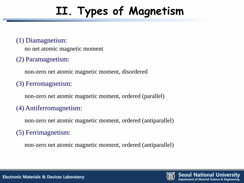
II. Types of Magnetism
11
Electronic Materials & Devices Laboratory Seoul National University Department of Material Science & Engineering (1) Diamagnetism: no net atomic magnetic moment (2) Paramagnetism: non-zero net atomic magnetic moment, disordered (3) Ferromagnetism: non-zero net atomic magnetic moment, ordered (parallel) (4) Antiferromagnetism: non-zero net atomic magnetic moment, ordered (antiparallel) (5) Ferrimagnetism: non-zero net atomic magnetic moment, ordered (antiparallel) II. Types of Magnetism
Transcript of II. Types of Magnetism
Electronic Materials & Devices Laboratory Seoul National University Department of Material Science & Engineering
(1) Diamagnetism:
no net atomic magnetic moment
(2) Paramagnetism:
non-zero net atomic magnetic moment, disordered
(3) Ferromagnetism:
non-zero net atomic magnetic moment, ordered (parallel)
(4) Antiferromagnetism:
non-zero net atomic magnetic moment, ordered (antiparallel)
(5) Ferrimagnetism:
non-zero net atomic magnetic moment, ordered (antiparallel)
II. Types of Magnetism

Electronic Materials & Devices Laboratory Seoul National University Department of Material Science & Engineering
Current, i = = =
An additional postulate, mυr = n(h/2π) (quantized angular momentum)
Then, magnetic moment due to orbital motion, μorbit = iA = πr2 = = for n =1
rc
e
2unit time
pointgiven a passing charge
▶ Origin of net atomic magnetic moment? - electron motion
orbital motion → electronic moment
spin motion
- nuclear motion → nuclear moment : normally, negligibly small
Orbit motion : Bohr model
Introduction
Electron ( charge = e-, mass me) r
v
Spin motion :
1925 yr. fine split in the optical
spectrum under a magnetic field :
Anomalous Zeeman Effect
Magnetic moment due to spin motion,
μspin =
= 0.927×10⁻²⁰ erg/Oe (or emu) :
→ A fundamental quantity called,
Bohr magneton, μB
mc
eh
4
rc
e
2 mc
eh
4
rc
e
2
c
er
2
Electronic Materials & Devices Laboratory Seoul National University Department of Material Science & Engineering
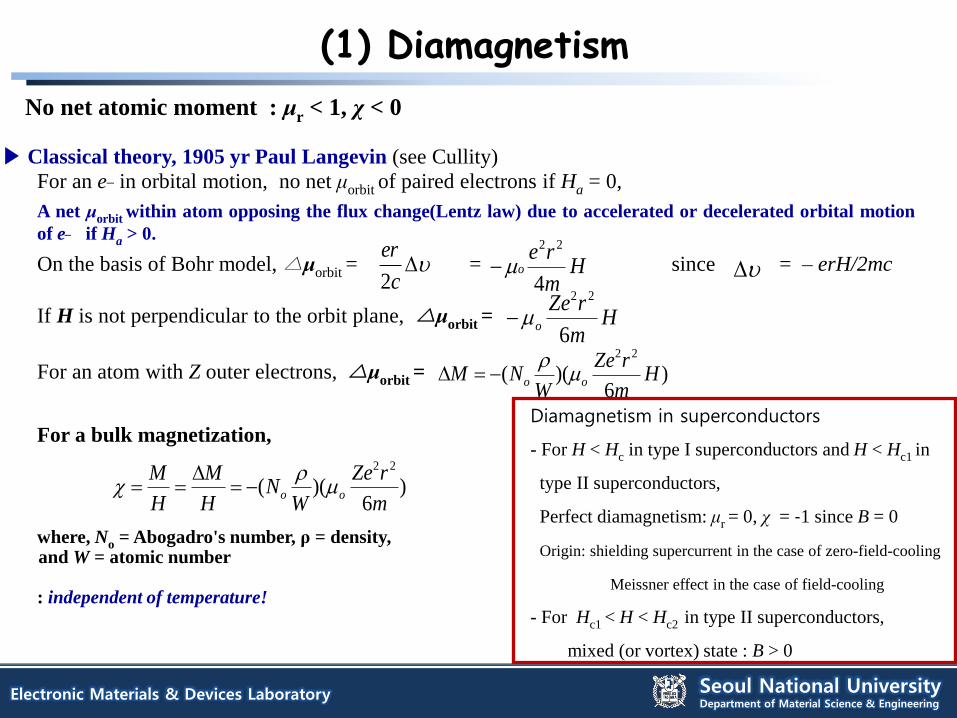
(1) Diamagnetism
No net atomic moment : μr < 1, χ < 0
▶ Classical theory, 1905 yr Paul Langevin (see Cullity)
For an e_ in orbital motion, no net μorbit of paired electrons if Ha = 0,
A net μorbit within atom opposing the flux change(Lentz law) due to accelerated or decelerated orbital motion
of e_ if Ha > 0.
On the basis of Bohr model, △μorbit = = since = – erH/2mc
If H is not perpendicular to the orbit plane, △μorbit =
For an atom with Z outer electrons, △μorbit =
For a bulk magnetization, where, No = Abogadro's number, ρ = density, and W = atomic number : independent of temperature!
Diamagnetism in superconductors
- For H < Hc in type I superconductors and H < Hc1 in
type II superconductors,
Perfect diamagnetism: μr = 0, χ = ‐1 since B = 0
Origin: shielding supercurrent in the case of zero-field-cooling
Meissner effect in the case of field-cooling
- For Hc1 < H < Hc2 in type II superconductors,
mixed (or vortex) state : B > 0
c
er
2H
m
reo
4
22
Hm
rZeo
6
22
)6
)((22
Hm
rZe
WNM oo
)6
)((22
m
rZe
WN
H
M
H
Moo
Electronic Materials & Devices Laboratory Seoul National University Department of Material Science & Engineering
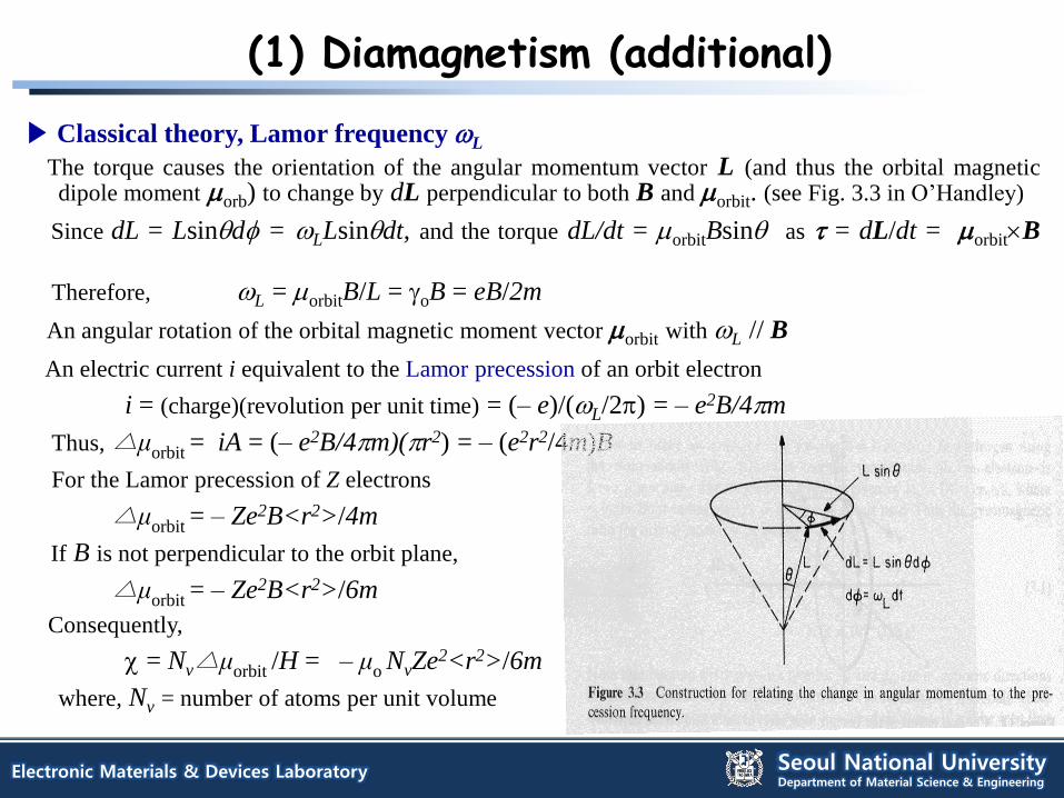
▶ Classical theory, Lamor frequency L
The torque causes the orientation of the angular momentum vector L (and thus the orbital magnetic dipole moment orb) to change by dL perpendicular to both B and orbit. (see Fig. 3.3 in O’Handley)
Since dL = Lsind = LLsindt, and the torque dL/dt = orbitBsin as = dL/dt = orbitB
Therefore, L = orbitB/L = oB = eB/2m
An angular rotation of the orbital magnetic moment vector orbit with L // B
An electric current i equivalent to the Lamor precession of an orbit electron
i = (charge)(revolution per unit time) = (– e)/(L/2) = – e2B/4m
Thus, △μorbit = iA = (– e2B/4m)(r2) = – (e2r2/4m)B
For the Lamor precession of Z electrons
△μorbit = – Ze2B<r2>/4m
If B is not perpendicular to the orbit plane,
△μorbit = – Ze2B<r2>/6m
Consequently,
= Nv△μorbit /H = – μo NvZe2<r2>/6m
where, Nv = number of atoms per unit volume
(1) Diamagnetism (additional)
Electronic Materials & Devices Laboratory Seoul National University Department of Material Science & Engineering
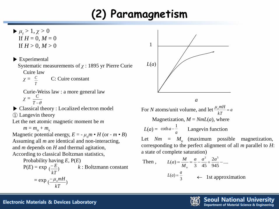
▶ μr > 1, χ > 0
If H = 0, M = 0
If H > 0, M > 0
▶ Experimental
Systematic measurements of χ : 1895 yr Pierre Curie
Cuire law
χ = C: Cuire constant
Curie-Weiss law : a more general law
χ =
▶ Classical theory : Localized electron model
① Langevin theory
Let the net atomic magnetic moment be m
m = mo + ms
Magnetic potential energy, E = - μom • H (or ‐ m • B)
Assuming all m are identical and non-interacting,
and m depends on H and thermal agitation,
According to classical Boltzman statistics,
Probability having E, P(E)
P(E) = exp k : Boltzmann constant
= exp
1
L(a)
a
For N atoms/unit volume, and let
Magnetization, M = NmL(a), where
L(a) = Langevin function
Let Nm = Mo (maximum possible magnetization,
corresponding to the perfect alignment of all m parallel to H:
a state of complete saturation)
Then ,
1st approximation
T
C
T
C
)(kT
E
)(kT
mHo
aa
1coth
akT
mHo
....945
2
453)(
52
aaa
M
MaL
o
3)(
aaL
(2) Paramagnetism

Electronic Materials & Devices Laboratory Seoul National University Department of Material Science & Engineering
② Weiss theory
Assuming the moments interact each other,
an interacting field He (called, molecular field or
exchange field)
He = αM : Weiss assumption
α is the molecular field constant
Htot = H + He
= H + αM
Since from Curie law
Htot =
Then,
θ = αC : measure of the strength of the interaction
→ leading to Curie-Weiss law
▶ Quantum theory
Localized electron model
Non-localized electron model : Pauli paramagnetism
(2) Paramagnetism (continued)
Remember the following;
Net atomic moment, m m = gμBJ
where, |J| = ħ
g(Lande splitting factor), 1 ≤ g ≤ 2 : empirical values
In general, Lande equation
If L = 0, J = S → g = 2 (only spin contribution)
If S = 0, J = L → g = 1 (only orbital contribution)
If J = ∞ : random orientation (classical)
T
C
H
M
tot
C
MT
T
C
MC
MT
M
MH
M
H
M
tot
)1( JJ
)1(2
)1()1()1(1
JJ
LLSSJJg
Electronic Materials & Devices Laboratory Seoul National University Department of Material Science & Engineering
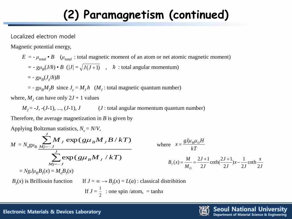
(2) Paramagnetism (continued)
Localized electron model
Magnetic potential energy,
E = ‐ μtotal • B (μtotal : total magnetic moment of an atom or net atomic magnetic moment)
= ‐ gμB(J/ħ) • B (|J| = , ħ : total angular momentum)
= ‐ gμB(Jz/ħ)B
= ‐ gμBMJB since Jz = MJ ħ (MJ : total magnetic quantum number)
where, MJ can have only 2J + 1 values
MJ = -J, -(J-1), ..., (J-1), J (J : total angular momentum quantum number)
Therefore, the average magnetization in B is given by
Applying Boltzman statistics, Nv = N/V,
M = NvgμB where
= NgJμBBJ(x) = MoBJ(x)
BJ(x) is Brilliouin function If J = ∞ → BJ(x) = L(a) : classical distribition
If J = : one spin /atom, = tanhx
kT
HgJx OB
J
x
Jx
J
J
J
J
M
MxB
O
J2
coth2
1)
2
12coth(
2
12)(
2
1
)1( JJ
J
JMj
JB
J
JMj
JBJ
kTMg
kTBMgM
)/exp(
)/exp(
Electronic Materials & Devices Laboratory Seoul National University Department of Material Science & Engineering
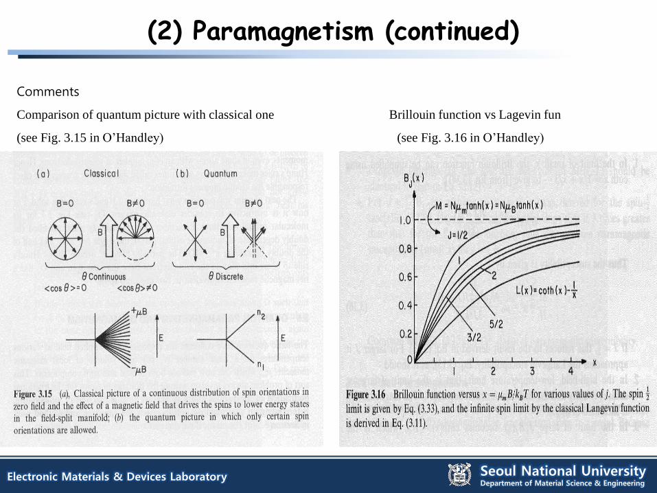
(2) Paramagnetism (continued)
Comments
Comparison of quantum picture with classical one Brillouin function vs Lagevin fun
(see Fig. 3.15 in O’Handley) (see Fig. 3.16 in O’Handley)
Electronic Materials & Devices Laboratory Seoul National University Department of Material Science & Engineering
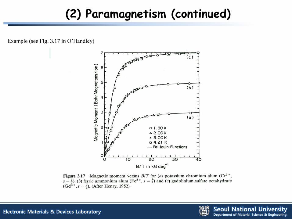
Example (see Fig. 3.17 in O’Handley)
(2) Paramagnetism (continued)
Electronic Materials & Devices Laboratory Seoul National University Department of Material Science & Engineering
(2) Paramagnetism (continued)
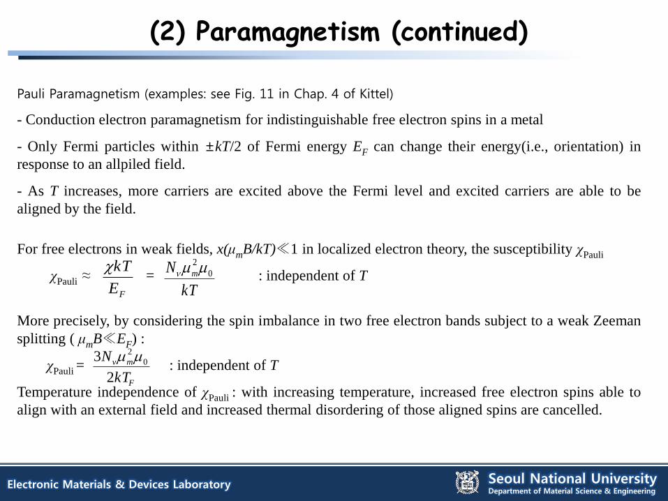
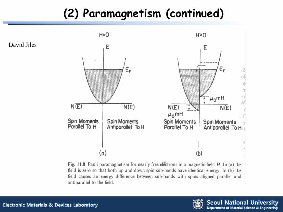
Pauli Paramagnetism (examples: see Fig. 11 in Chap. 4 of Kittel)
- Conduction electron paramagnetism for indistinguishable free electron spins in a metal
- Only Fermi particles within ±kT/2 of Fermi energy EF can change their energy(i.e., orientation) in
response to an allpiled field.
- As T increases, more carriers are excited above the Fermi level and excited carriers are able to be
aligned by the field.
For free electrons in weak fields, x(μmB/kT)≪1 in localized electron theory, the susceptibility χPauli
χPauli ≈ = : independent of T
More precisely, by considering the spin imbalance in two free electron bands subject to a weak Zeeman
splitting ( μmB≪EF) :
χPauli = : independent of T
Temperature independence of χPauli : with increasing temperature, increased free electron spins able to
align with an external field and increased thermal disordering of those aligned spins are cancelled.
FE
kT
kT
N m 0
2
F
mv
kT
N
2
3 0
2
Electronic Materials & Devices Laboratory Seoul National University Department of Material Science & Engineering
(2) Paramagnetism (continued)
David Jiles