I. II. ψ and probability - Viện Vật lý · Quantum Mechanics I Sally Seidel Primary textbook:...
101
Quantum Mechanics I Sally Seidel Primary textbook: “Quantum Mechanics” by Amit Goswami Please read Chapter 1, Sections 4-9 Outline I. What you should recall from previous courses II. Motivation for the Schroedinger Equation III. The relationship between wavefunction ψ and probability IV. Normalization V. Expectation values VI. Phases in the wavefunction 1
-
Upload
hoanghuong -
Category
Documents
-
view
215 -
download
0
Transcript of I. II. ψ and probability - Viện Vật lý · Quantum Mechanics I Sally Seidel Primary textbook:...
Quantum Mechanics I Sally Seidel Primary textbook: “Quantum Mechanics” by Amit Goswami
Please read Chapter 1, Sections 4-9
Outline I. What you should recall from previous courses II. Motivation for the Schroedinger Equation III. The relationship between wavefunction ψ and probability IV. Normalization V. Expectation values VI. Phases in the wavefunction
1
2
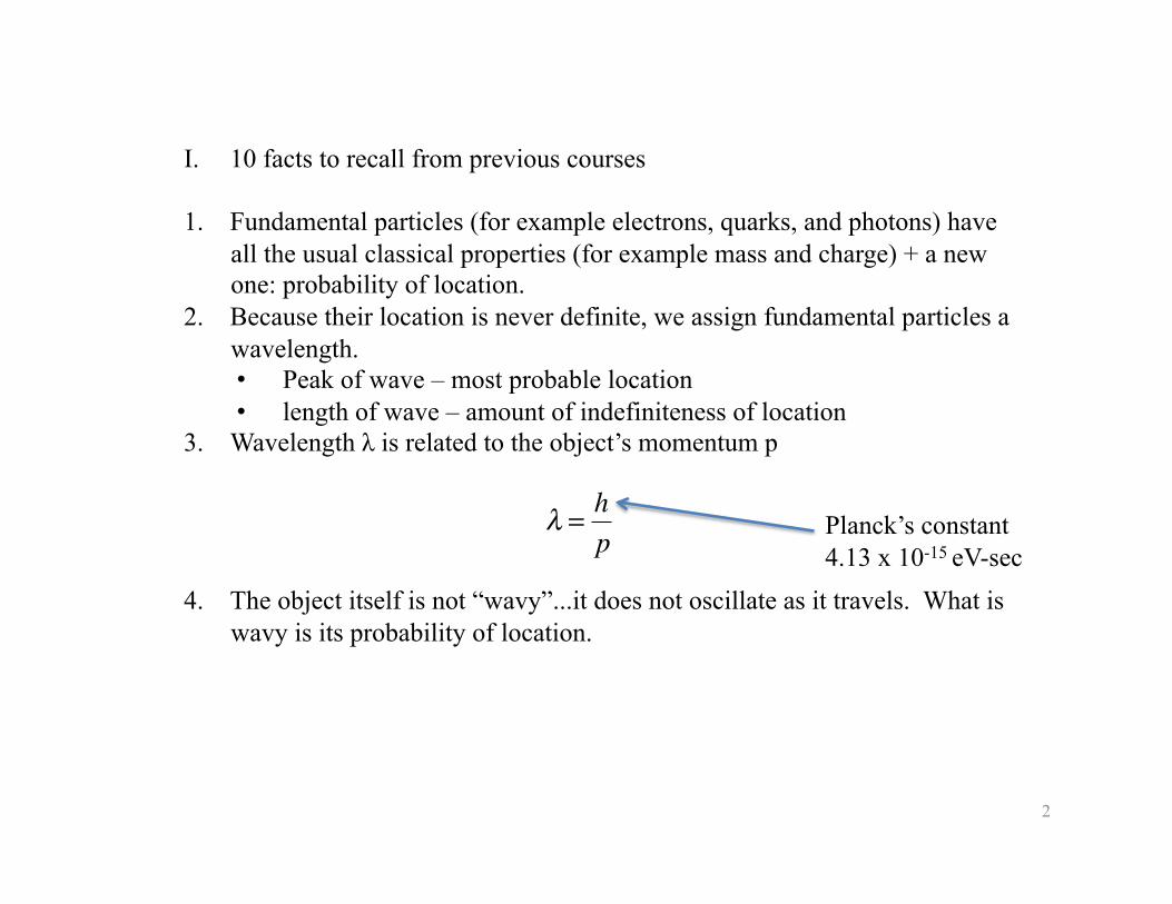
I. 10 facts to recall from previous courses
1. Fundamental particles (for example electrons, quarks, and photons) have all the usual classical properties (for example mass and charge) + a new one: probability of location.
2. Because their location is never definite, we assign fundamental particles a wavelength. • Peak of wave – most probable location • length of wave – amount of indefiniteness of location
3. Wavelength λ is related to the object’s momentum p
4. The object itself is not “wavy”...it does not oscillate as it travels. What is wavy is its probability of location.
�
λ = hp Planck’s constant
4.13 x 10⁻¹⁵ eV-sec
3
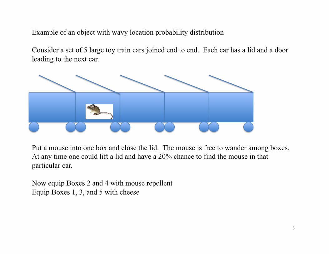
Example of an object with wavy location probability distribution
Consider a set of 5 large toy train cars joined end to end. Each car has a lid and a door leading to the next car.
Put a mouse into one box and close the lid. The mouse is free to wander among boxes. At any time one could lift a lid and have a 20% chance to find the mouse in that particular car.
Now equip Boxes 2 and 4 with mouse repellent Equip Boxes 1, 3, and 5 with cheese
4
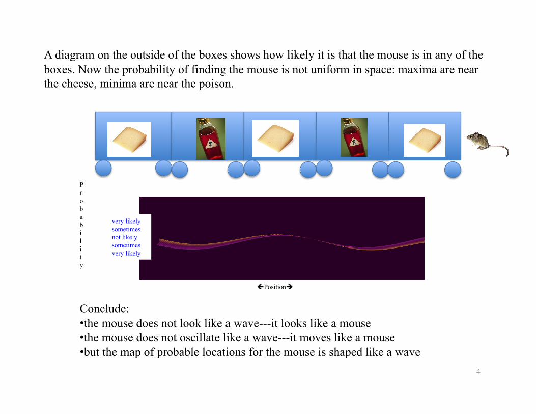
A diagram on the outside of the boxes shows how likely it is that the mouse is in any of the boxes. Now the probability of finding the mouse is not uniform in space: maxima are near the cheese, minima are near the poison.
very likely sometimes not likely sometimes very likely
Probability
Position
Conclude: • the mouse does not look like a wave---it looks like a mouse • the mouse does not oscillate like a wave---it moves like a mouse • but the map of probable locations for the mouse is shaped like a wave
5
The situation for the electron or photon is almost the same, except • for the mouse example, Probability = Amplitude • for the electron (or any quantum mechanical object,
Probability = (Amplitude)*(Amplitude)
5. As with all waves, wavelength λ is related to frequency υ:
λυ = velocity of wave 6. QM says that the λ ( or υ) is also related to the energy:
E=hυ $
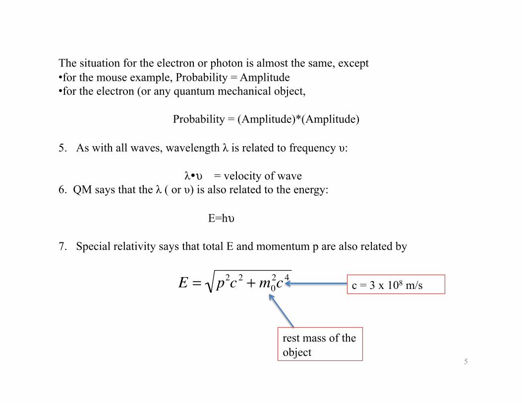
7. Special relativity says that total E and momentum p are also related by
�
E = p2c 2 + m02c 4
rest mass of the object
c = 3 x 10⁸ m/s
6
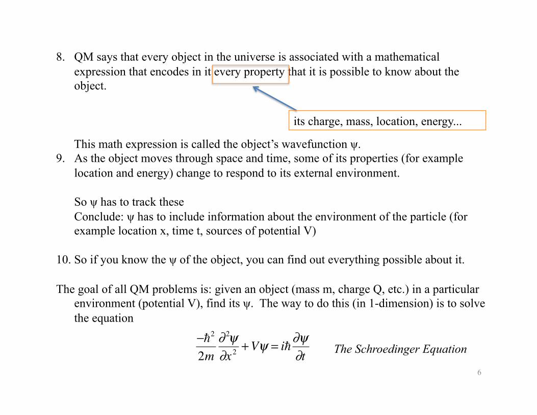
8. QM says that every object in the universe is associated with a mathematical expression that encodes in it every property that it is possible to know about the object.
This math expression is called the object’s wavefunction ψ. 9. As the object moves through space and time, some of its properties (for example
location and energy) change to respond to its external environment.
So ψ has to track these Conclude: ψ has to include information about the environment of the particle (for example location x, time t, sources of potential V)
10. So if you know the ψ of the object, you can find out everything possible about it.
The goal of all QM problems is: given an object (mass m, charge Q, etc.) in a particular environment (potential V), find its ψ. The way to do this (in 1-dimension) is to solve the equation
its charge, mass, location, energy...
�
−2
2m∂ 2ψ∂x 2
+Vψ = i∂ψ∂t The Schroedinger Equation
7
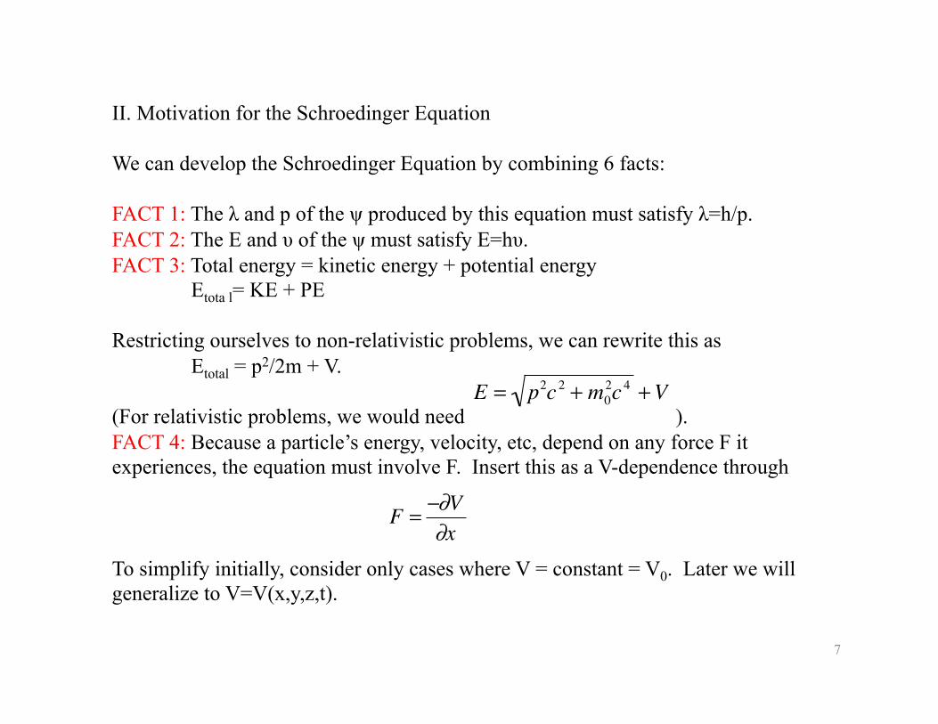
II. Motivation for the Schroedinger Equation
We can develop the Schroedinger Equation by combining 6 facts:
FACT 1: The λ and p of the ψ produced by this equation must satisfy λ=h/p. FACT 2: The E and υ of the ψ must satisfy E=hυ. FACT 3: Total energy = kinetic energy + potential energy
Etota l= KE + PE
Restricting ourselves to non-relativistic problems, we can rewrite this as Etotal = p2/2m + V.
(For relativistic problems, we would need ). FACT 4: Because a particle’s energy, velocity, etc, depend on any force F it experiences, the equation must involve F. Insert this as a V-dependence through
To simplify initially, consider only cases where V = constant = V0. Later we will generalize to V=V(x,y,z,t).
�
E = p2c 2 + m02c 4 +V
�
F = −∂V∂x
8
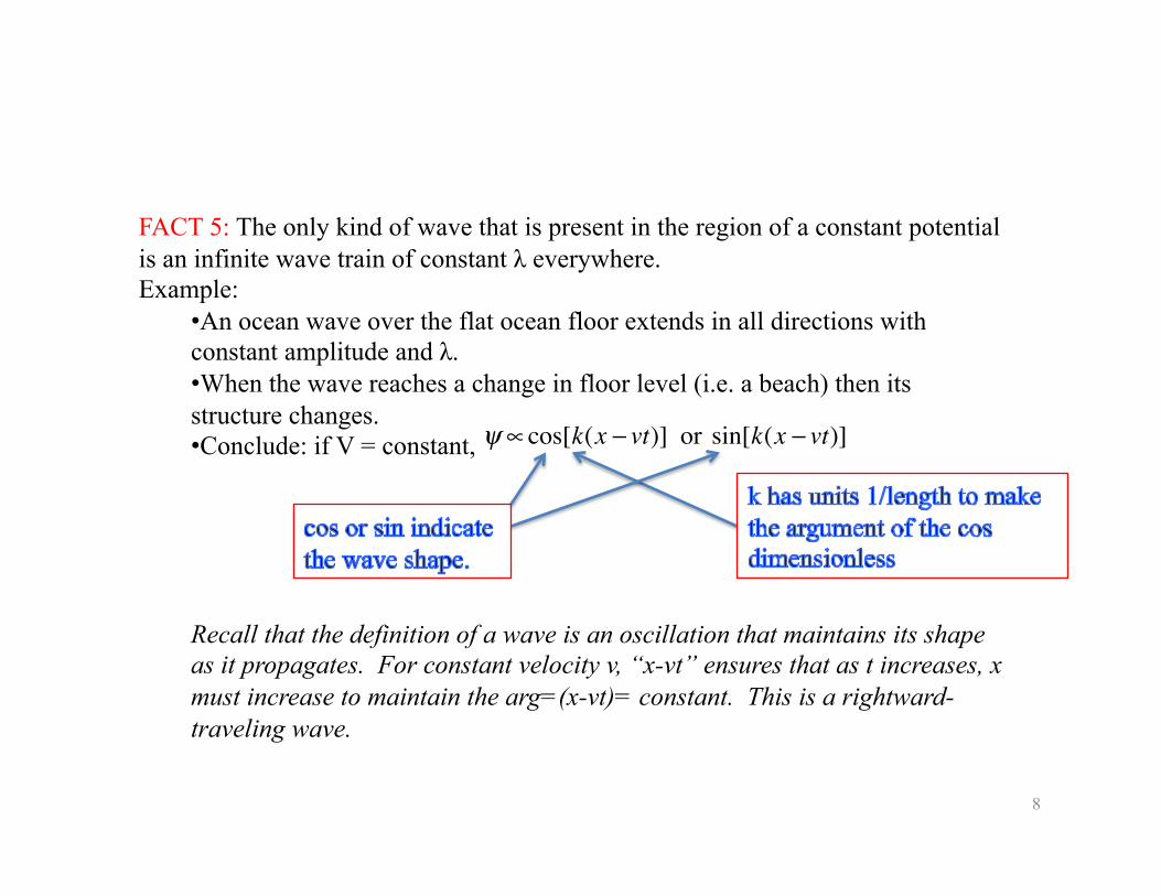
FACT 5: The only kind of wave that is present in the region of a constant potential is an infinite wave train of constant λ everywhere. Example:
• An ocean wave over the flat ocean floor extends in all directions with constant amplitude and λ. • When the wave reaches a change in floor level (i.e. a beach) then its structure changes. • Conclude: if V = constant,
Recall that the definition of a wave is an oscillation that maintains its shape as it propagates. For constant velocity v, “x-vt” ensures that as t increases, x must increase to maintain the arg=(x-vt)= constant. This is a rightward-traveling wave.
�
ψ ∝cos[k(x − vt)] or sin[k(x − vt)]
9
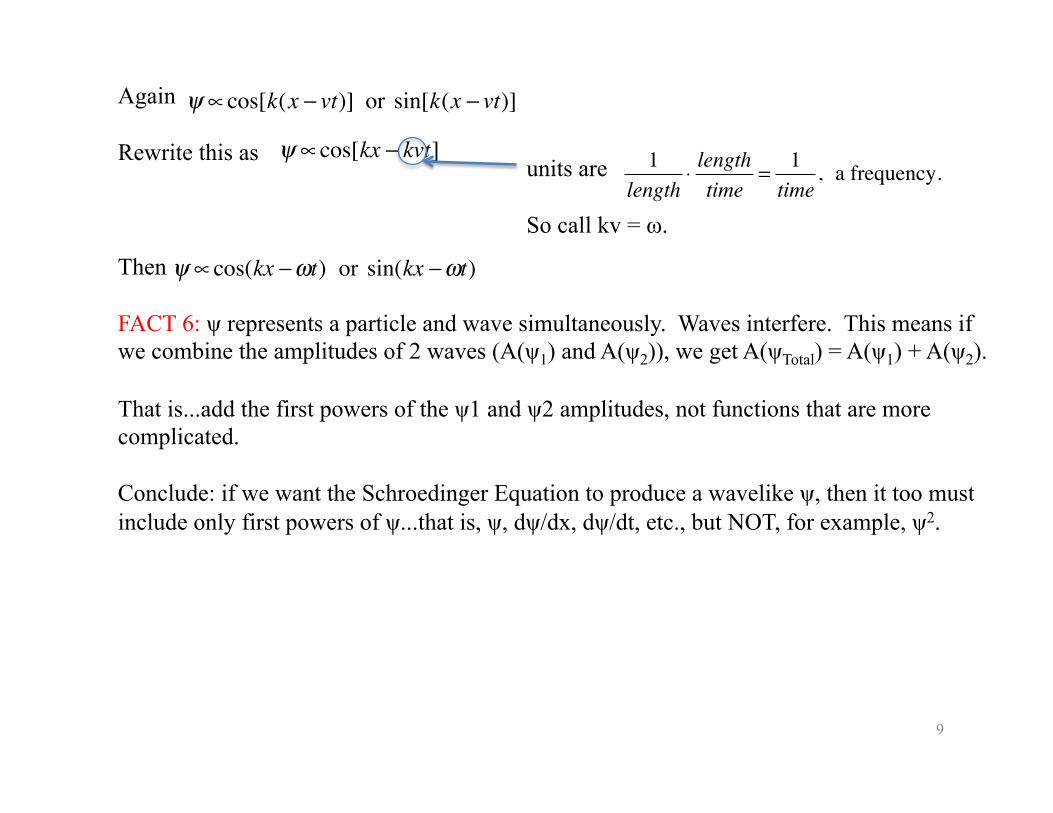
Again
Rewrite this as
Then
FACT 6: ψ represents a particle and wave simultaneously. Waves interfere. This means if we combine the amplitudes of 2 waves (A(ψ1) and A(ψ2)), we get A(ψTotal) = A(ψ1) + A(ψ2).
That is...add the first powers of the ψ1 and ψ2 amplitudes, not functions that are more complicated.
Conclude: if we want the Schroedinger Equation to produce a wavelike ψ, then it too must include only first powers of ψ...that is, ψ, dψ/dx, dψ/dt, etc., but NOT, for example, ψ2.
�
ψ ∝cos[k(x − vt)] or sin[k(x − vt)]
�
ψ ∝cos[kx − kvt] units are
So call kv = ω.
�
1length
⋅ lengthtime
= 1time
, a frequency.
�
ψ ∝cos(kx −ωt) or sin(kx −ωt)
10
�
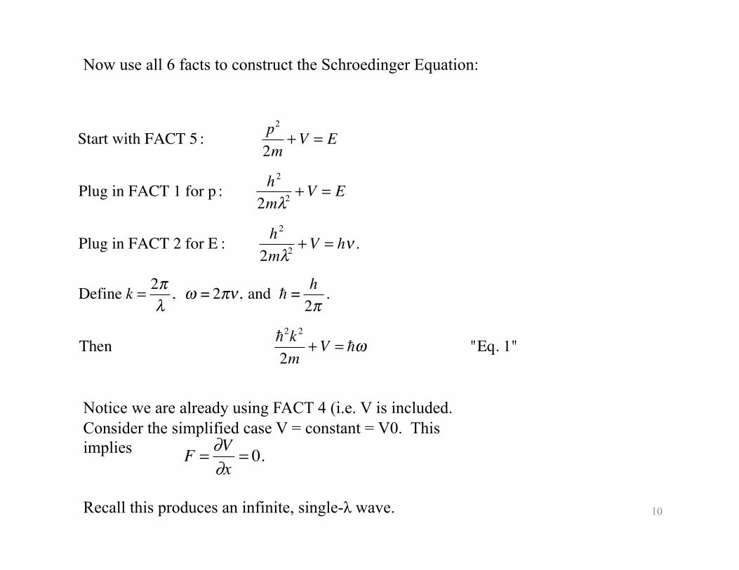
Start with FACT 5 : p2
2m+V = E
Plug in FACT 1 for p : h2
2mλ2 +V = E
Plug in FACT 2 for E : h2
2mλ2 +V = hν .
Define k = 2πλ
, ω = 2πν, and = h2π
.
Then 2k 2
2m+V = ω "Eq. 1"
Now use all 6 facts to construct the Schroedinger Equation:
Notice we are already using FACT 4 (i.e. V is included. Consider the simplified case V = constant = V0. This implies
Recall this produces an infinite, single-λ wave.
�
F = ∂V∂x
= 0.
11
�
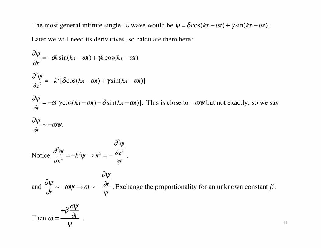
The most general infinite single -υ wave would be ψ = δcos(kx −ωt) + γ sin(kx −ωt).
Later we will need its derivatives, so calculate them here :
∂ψ∂x
= −δk sin(kx −ωt) + γk cos(kx −ωt)
∂ 2ψ∂x 2 = −k 2[δcos(kx −ωt) + γ sin(kx −ωt)]
∂ψ∂t
= −ω[γ cos(kx −ωt) −δ sin(kx −ωt)]. This is close to -ωψ but not exactly, so we say
∂ψ∂t
~ −ωψ.
Notice ∂2ψ
∂x 2 = −k 2ψ → k 2 = −
∂ 2ψ∂x 2
ψ.
and ∂ψ∂t
~ −ωψ →ω ~ −
∂ψ∂tψ
. Exchange the proportionality for an unknown constant β .
Then ω =+β ∂ψ
∂tψ
.
12
�
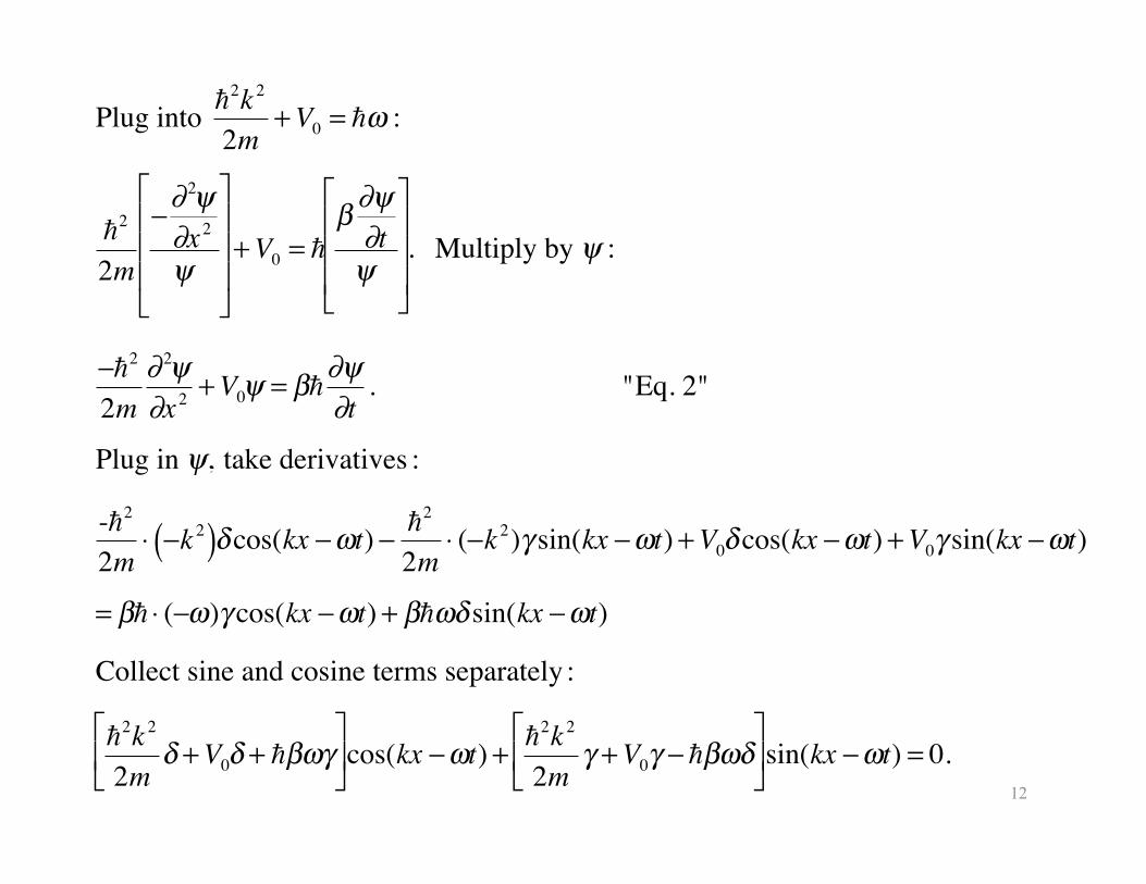
Plug into 2k 2
2m+V0 = ω :
2
2m
−∂2ψ
∂x 2
ψ
⎡
⎣
⎢ ⎢ ⎢
⎤
⎦
⎥ ⎥ ⎥
+V0 = β ∂ψ∂tψ
⎡
⎣
⎢ ⎢ ⎢
⎤
⎦
⎥ ⎥ ⎥ . Multiply by ψ :
−2
2m∂ 2ψ∂x 2 +V0ψ = β∂ψ
∂t. "Eq. 2"
Plug in ψ, take derivatives :
-2
2m⋅ −k 2( )δcos(kx −ωt) −
2
2m⋅ (−k 2)γ sin(kx −ωt) +V0δcos(kx −ωt) +V0γ sin(kx −ωt)
= β ⋅ (−ω)γ cos(kx −ωt) + βωδ sin(kx −ωt)
Collect sine and cosine terms separately :
2k 2
2mδ +V0δ + βωγ
⎡
⎣ ⎢
⎤
⎦ ⎥ cos(kx −ωt) +
2k 2
2mγ +V0γ − βωδ
⎡
⎣ ⎢
⎤
⎦ ⎥ sin(kx −ωt) = 0.
13
�
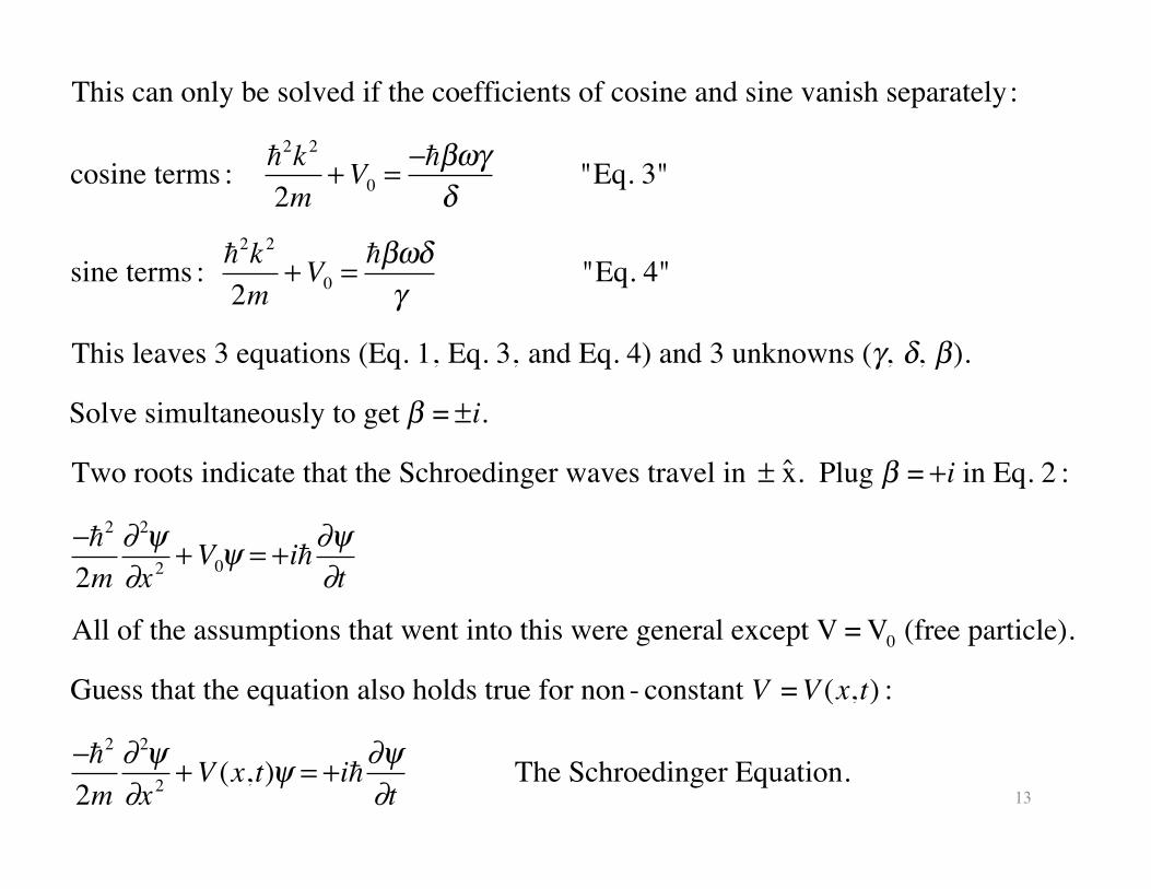
This can only be solved if the coefficients of cosine and sine vanish separately:
cosine terms : 2k 2
2m+V0 = −βωγ
δ "Eq. 3"
sine terms : 2k 2
2m+V0 = βωδ
γ "Eq. 4"
This leaves 3 equations (Eq. 1, Eq. 3, and Eq. 4) and 3 unknowns (γ, δ, β).
Solve simultaneously to get β = ±i.
Two roots indicate that the Schroedinger waves travel in ± ˆ x . Plug β = +i in Eq. 2 :
−2
2m∂ 2ψ∂x 2 +V0ψ = +i∂ψ
∂t
All of the assumptions that went into this were general except V = V0 (free particle).
Guess that the equation also holds true for non - constant V =V (x, t) :
−2
2m∂ 2ψ∂x 2 +V (x,t)ψ = +i∂ψ
∂t The Schroedinger Equation.
14
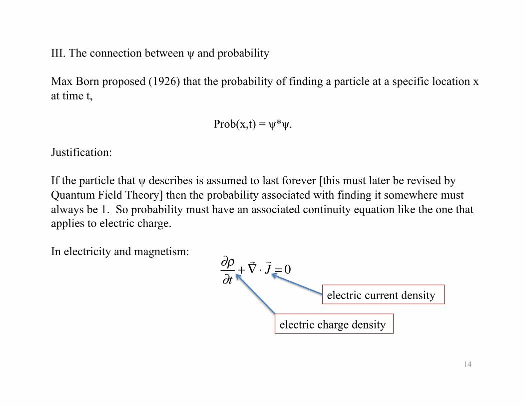
III. The connection between ψ and probability
Max Born proposed (1926) that the probability of finding a particle at a specific location x at time t,
Prob(x,t) = ψ*ψ.
Justification:
If the particle that ψ describes is assumed to last forever [this must later be revised by Quantum Field Theory] then the probability associated with finding it somewhere must always be 1. So probability must have an associated continuity equation like the one that applies to electric charge.
In electricity and magnetism:
�
∂ρ∂t
+ ∇ ⋅ J = 0
electric current density
electric charge density
15
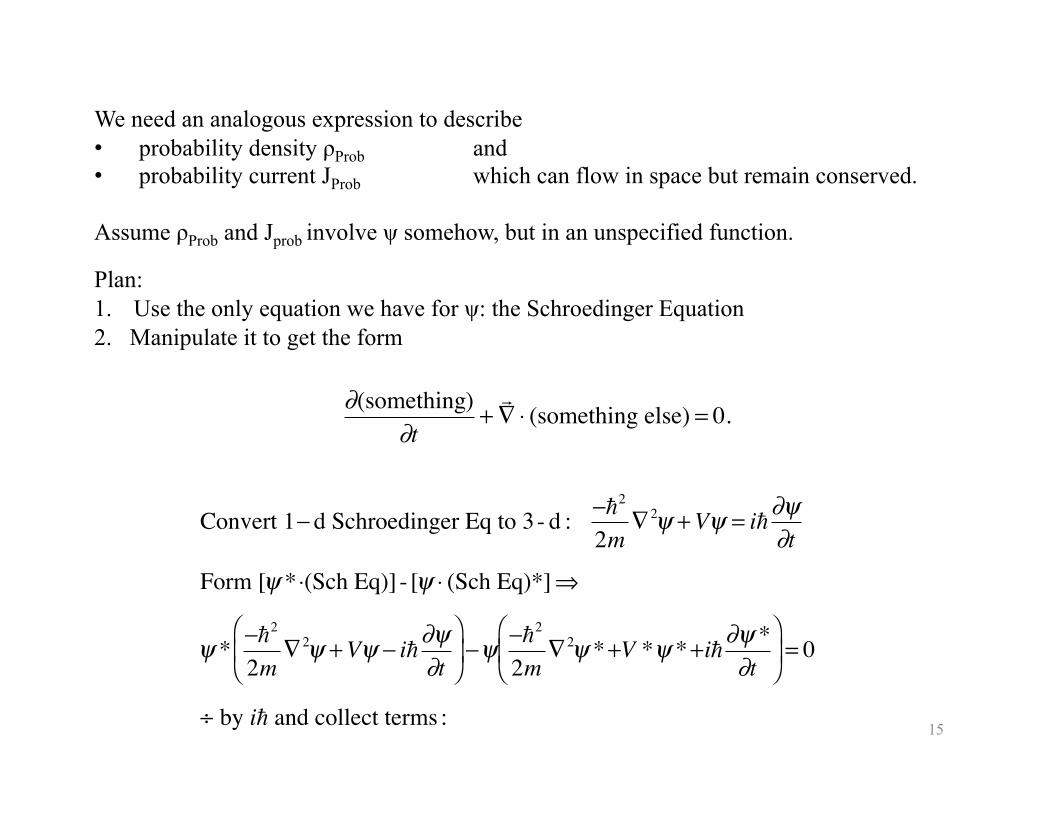
We need an analogous expression to describe • probability density ρProb and • probability current JProb which can flow in space but remain conserved.
Assume ρProb and Jprob involve ψ somehow, but in an unspecified function.
Plan: 1. Use the only equation we have for ψ: the Schroedinger Equation 2. Manipulate it to get the form
�
∂(something)∂t
+ ∇ ⋅ (something else) = 0.
�
Convert 1− d Schroedinger Eq to 3 - d : −2
2m∇2ψ +Vψ = i∂ψ
∂t
Form [ψ * ⋅(Sch Eq)] - [ψ ⋅ (Sch Eq)*]⇒
ψ * −2
2m∇2ψ +Vψ − i∂ψ
∂t⎛
⎝ ⎜
⎞
⎠ ⎟ −ψ
−2
2m∇2ψ * +V *ψ * +i∂ψ *
∂t⎛
⎝ ⎜
⎞
⎠ ⎟ = 0
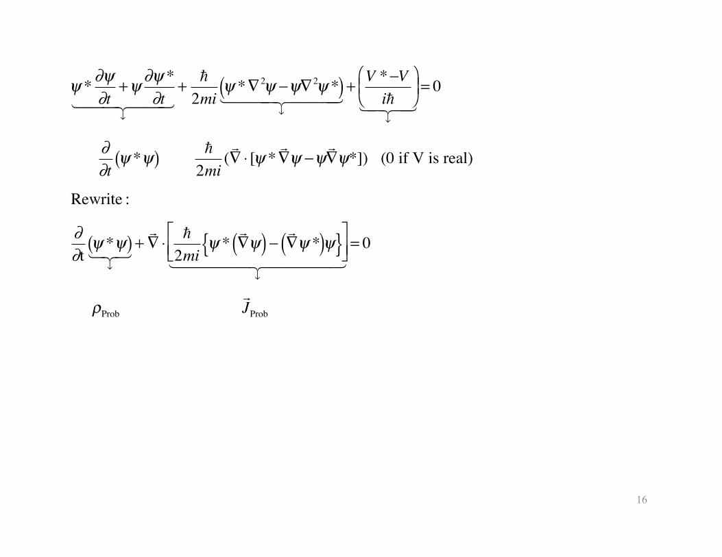
÷ by i and collect terms :
16
�
ψ * ∂ψ∂t
+ψ ∂ψ *∂t
↓
+
2miψ *∇2ψ −ψ∇2ψ *( )
↓
+ V *−Vi
⎛ ⎝ ⎜
⎞ ⎠ ⎟
↓
= 0
∂∂t
ψ *ψ( ) 2mi
( ∇ ⋅ [ψ *
∇ ψ −ψ
∇ ψ*]) (0 if V is real)
Rewrite :
∂∂t
ψ *ψ( )↓
+ ∇ ⋅
2miψ * ∇ ψ( ) − ∇ ψ *( )ψ{ }⎡
⎣ ⎢ ⎤ ⎦ ⎥
↓
= 0
ρProb J Prob
17
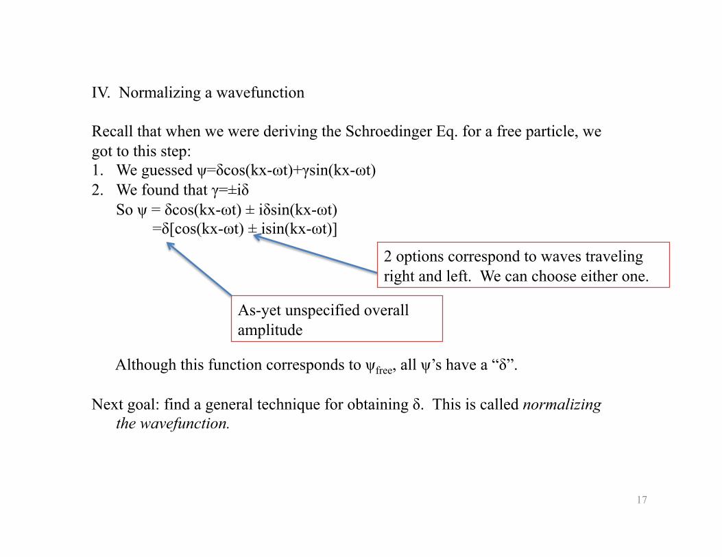
IV. Normalizing a wavefunction
Recall that when we were deriving the Schroedinger Eq. for a free particle, we got to this step: 1. We guessed ψ=δcos(kx-ωt)+γsin(kx-ωt) 2. We found that γ=±iδ
So ψ = δcos(kx-ωt) ± iδsin(kx-ωt) =δ[cos(kx-ωt) ± isin(kx-ωt)]
Although this function corresponds to ψfree, all ψ’s have a “δ”.
Next goal: find a general technique for obtaining δ. This is called normalizing the wavefunction.
2 options correspond to waves traveling right and left. We can choose either one.
As-yet unspecified overall amplitude
18
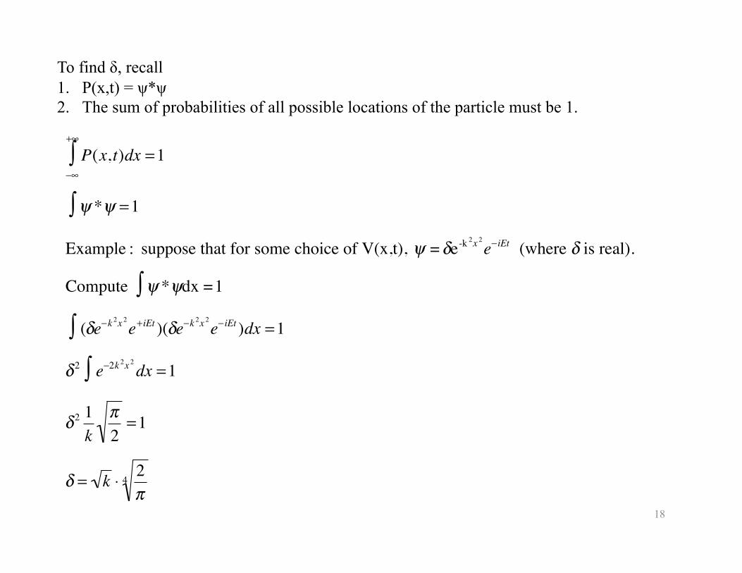
To find δ, recall 1. P(x,t) = ψ*ψ 2. The sum of probabilities of all possible locations of the particle must be 1.
�
P(x, t)dx = 1−∞
+∞
∫
ψ *ψ = 1∫Example : suppose that for some choice of V(x,t), ψ =δe-k 2x 2
e−iEt (where δ is real).
Compute ψ *ψdx =1∫(δe−k
2x 2
e+iEt )(δe−k2x 2
e− iEt )dx = 1∫δ 2 e−2k 2x 2
dx = 1∫
δ 2 1k
π2
= 1
δ = k ⋅ 2π
4
19
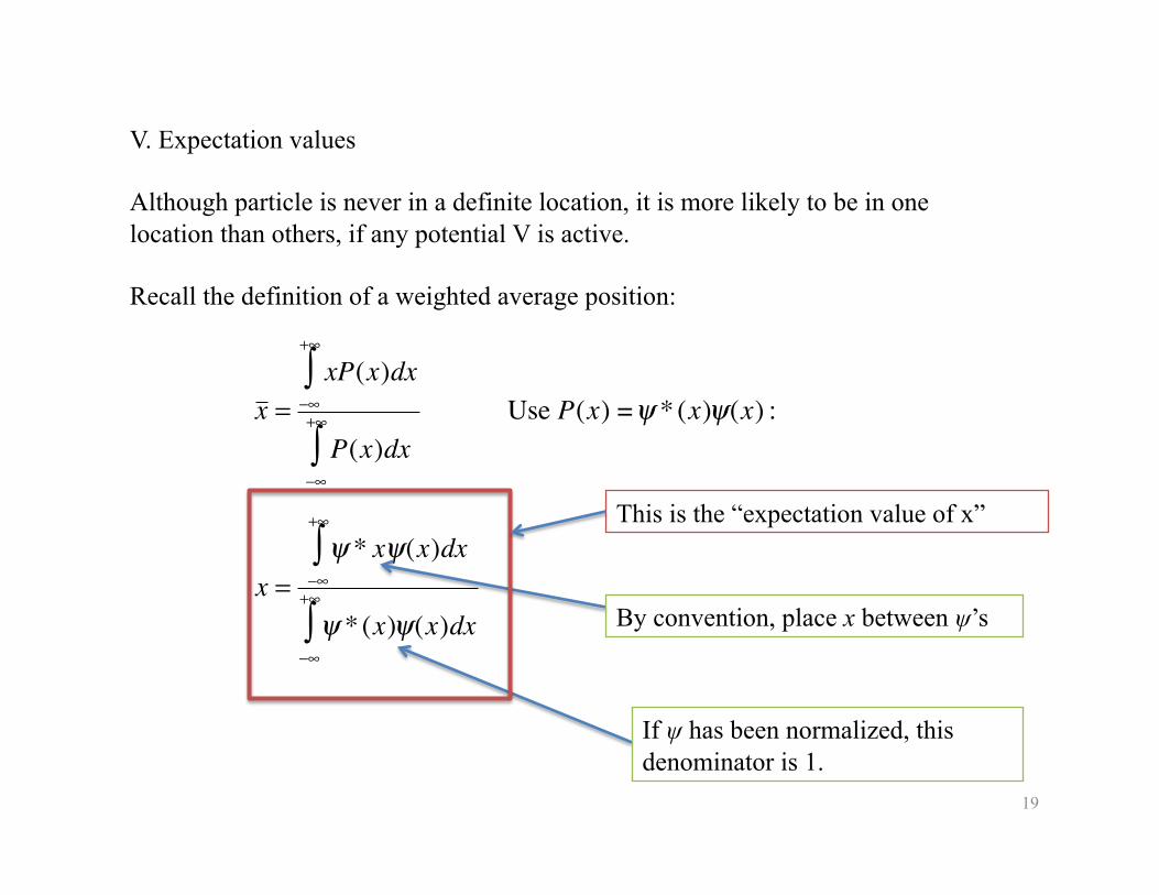
V. Expectation values
Although particle is never in a definite location, it is more likely to be in one location than others, if any potential V is active.
Recall the definition of a weighted average position:
�
x =xP(x)dx
−∞
+∞
∫
P(x)dx−∞
+∞
∫ Use P(x) =ψ * (x)ψ(x) :
x =ψ * xψ(x)dx
−∞
+∞
∫
ψ * (x)ψ(x)dx−∞
+∞
∫ By convention, place x between ψ’s
If ψ has been normalized, this denominator is 1.
This is the “expectation value of x”
20
�
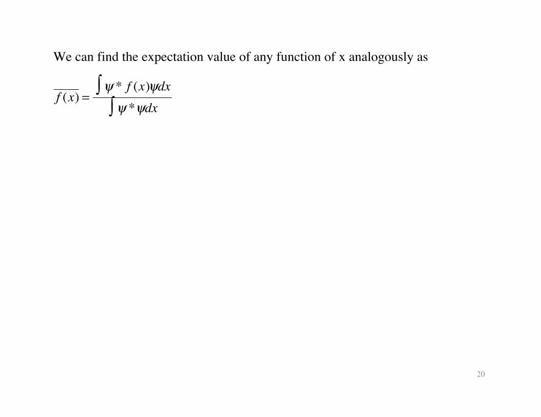
We can find the expectation value of any function of x analogously as
f (x) =ψ * f (x)ψdx∫ψ *ψdx∫
21
Please read Goswami Chapter 2.
Outline I. Normalizing a free particle wavefunction II. Acceptable mathematical forms of ψ III. The phase of the wavefunction IV. The effect of a potential on a wave V. Wave packets VI. The Uncertainty Principle
22
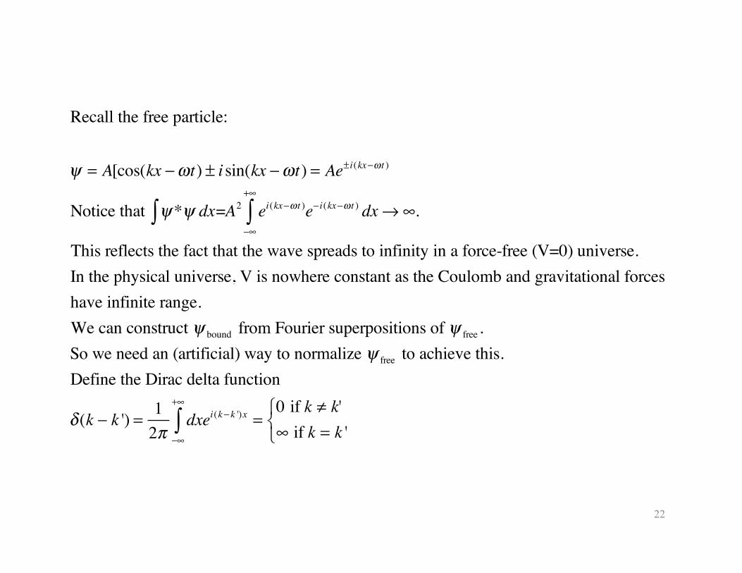
Recall the free particle:
ψ = A[cos(kx −ωt) ± i sin(kx −ωt) = Ae± i(kx−ω t )
Notice that ψ*ψ dx=∫ A2 ei(kx−ω t )e− i(kx−ω t ) dx→∞.−∞
+∞
∫This reflects the fact that the wave spreads to infinity in a force-free (V=0) universe.In the physical universe, V is nowhere constant as the Coulomb and gravitational forces have infinite range. We can construct ψ bound from Fourier superpositions of ψ free .So we need an (artificial) way to normalize ψ free to achieve this.Define the Dirac delta function
δ (k − k ') = 12π
dxei(k− k ')x =0 if k ≠ k'∞ if k = k '
⎧⎨⎩−∞
+∞
∫
23
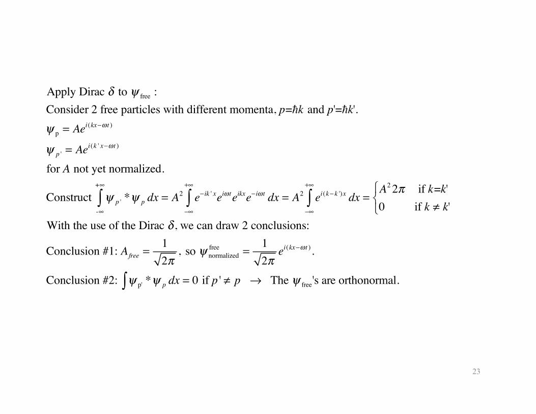
Apply Dirac δ to ψ free :Consider 2 free particles with different momenta, p=k and p'=k'.ψ p = Ae
i(kx−ω t )
ψ p ' = Aei(k ' x−ω t )
for A not yet normalized.
Construct ψ p ' *ψ p dx = A2 e− ik ' xeiω teikxe− iω t dx = A2 ei(k− k ')x dx
−∞
+∞
∫−∞
+∞
∫-∞
+∞
∫ =A2 2π if k=k'0 if k ≠ k'
⎧⎨⎩
With the use of the Dirac δ , we can draw 2 conclusions:
Conclusion #1: Afree =12π
, so ψ normalizedfree =
12π
ei(kx−ω t ).
Conclusion #2: ψ p' *ψ p dx = 0 if p ' ≠ p → The ψ free's are orthonormal.∫
24
II Acceptable mathematical forms of wavefunctions
ψ must be normalizable, so must be a convergent integral-
i.e., at minimum, require
A ψ that satisfies this is called “square integrable.”
�
ψ *ψdx−∞
+∞
∫
�
ψ *ψdx−∞
+∞
∫ < ∞
25
III The phase of the wavefunction
FACT 1: We cannot observe ψ itself; we only observe ψ*ψ. So overall phase is physically irrelevant.
FACT 2: The relative phase of two ψ’s in the same region affects the probability distribution, which is measurement, through superposition:
Suppose ψ1 = Aeiα and ψ2 = Beiβ, where A and B are real. ψtot = Aeiα + Beiβ = eiα[A+Bei(β-α)], so Prob=ψ*ψ=[A+Bei(β-α)][A+Be-i(β-α)]=A2+B2+AB[ei(β-α)+e-i(β-α)]= A2 + B2 + 2ABcos(β-α)
FACT 3: The flow of probability depends on both the amplitude and the phase: Consider ψ=Aeiα where A can be complex.
26
�
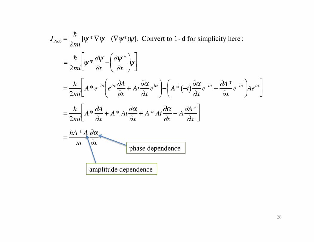
JProb =
2mi[ψ *∇ψ − (∇ψ*)ψ]. Convert to 1- d for simplicity here :
=
2miψ * ∂ψ
∂x− ∂ψ *
∂x⎛ ⎝ ⎜
⎞ ⎠ ⎟ ψ
⎡ ⎣ ⎢
⎤ ⎦ ⎥
=
2miA*e− iα eiα ∂A
∂x+ Ai∂α
∂xeiα
⎛ ⎝ ⎜
⎞ ⎠ ⎟ − A* −i( )∂α
∂xe− iα + ∂A*
∂xe− iα
⎛ ⎝ ⎜
⎞ ⎠ ⎟ Aeiα
⎡ ⎣ ⎢
⎤ ⎦ ⎥
=
2miA* ∂A
∂x+ A* Ai∂α
∂x+ A* Ai∂α
∂x− A∂A*
∂x⎡ ⎣ ⎢
⎤ ⎦ ⎥
= A* Am
∂α∂x
phase dependence
amplitude dependence
27
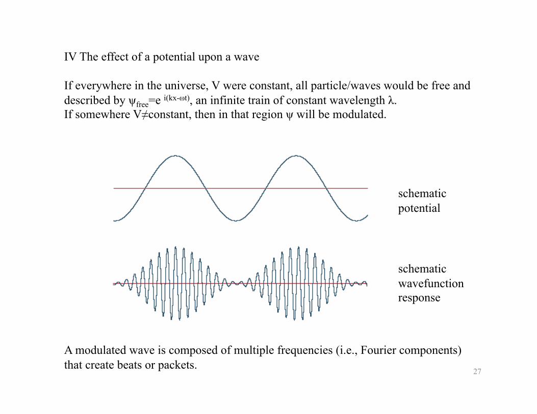
IV The effect of a potential upon a wave
If everywhere in the universe, V were constant, all particle/waves would be free and described by ψfree=e i(kx-ωt), an infinite train of constant wavelength λ. If somewhere V≠constant, then in that region ψ will be modulated.
schematic potential
schematic wavefunction response
A modulated wave is composed of multiple frequencies (i.e., Fourier components) that create beats or packets.
28
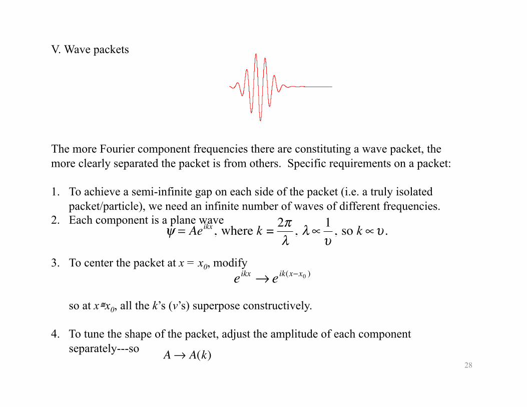
V. Wave packets
The more Fourier component frequencies there are constituting a wave packet, the more clearly separated the packet is from others. Specific requirements on a packet:
1. To achieve a semi-infinite gap on each side of the packet (i.e. a truly isolated packet/particle), we need an infinite number of waves of different frequencies.
2. Each component is a plane wave
3. To center the packet at x = x0, modify
so at x≅x0, all the k’s (ν’s) superpose constructively.
4. To tune the shape of the packet, adjust the amplitude of each component separately---so
�
ψ = Aeikx, where k = 2πλ
, λ ∝ 1υ
, so k ∝υ .
�
eikx → eik(x−x0 )
�
A→ A(k)
29
�
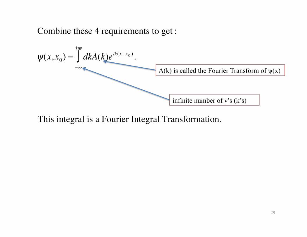
Combine these 4 requirements to get :
ψ(x,x0) = dkA(k)eik(x−x0 ).−∞
+∞
∫
This integral is a Fourier Integral Transformation.
A(k) is called the Fourier Transform of ψ(x)
infinite number of ν’s (k’s)
30
VI. The Uncertainty Principle
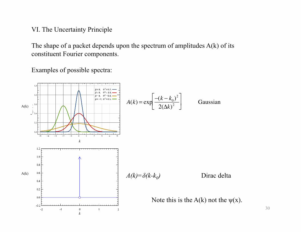
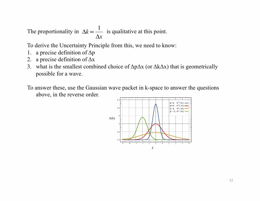
The shape of a packet depends upon the spectrum of amplitudes A(k) of its constituent Fourier components.
Examples of possible spectra:
Note this is the A(k) not the ψ(x).
k
A(k)
�
A(k) = exp −(k − k0)2
2(Δk)2
⎡
⎣ ⎢
⎤
⎦ ⎥ Gaussian
k
A(k) A(k)=δ(k-k0) Dirac delta
31
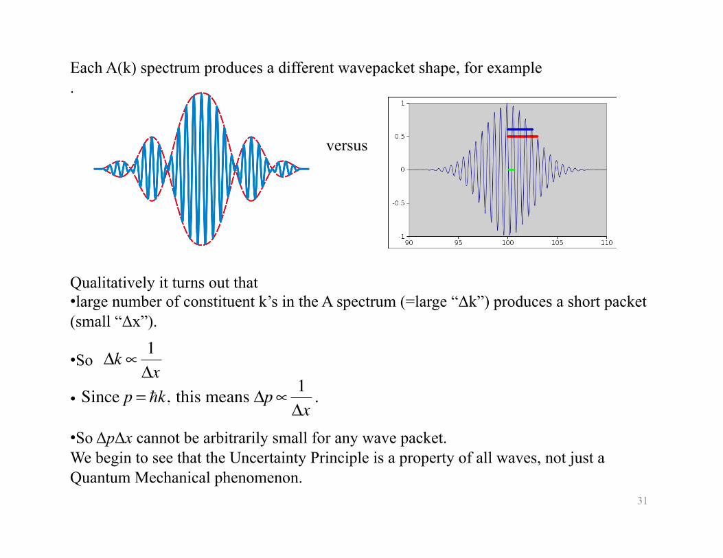
Each A(k) spectrum produces a different wavepacket shape, for example .
versus
Qualitatively it turns out that • large number of constituent k’s in the A spectrum (=large “Δk”) produces a short packet (small “Δx”).
• So
•
• So ΔpΔx cannot be arbitrarily small for any wave packet. We begin to see that the Uncertainty Principle is a property of all waves, not just a Quantum Mechanical phenomenon.
�
Δk ∝ 1Δx
�
Since p = k, this means Δp∝ 1Δx
.
32
The proportionality in is qualitative at this point.
To derive the Uncertainty Principle from this, we need to know: 1. a precise definition of Δp 2. a precise definition of Δx 3. what is the smallest combined choice of ΔpΔx (or ΔkΔx) that is geometrically
possible for a wave.
To answer these, use the Gaussian wave packet in k-space to answer the questions above, in the reverse order.
�
Δk ∝ 1Δx
k
A(k)
33
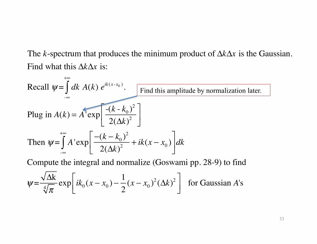
The k-spectrum that produces the minimum product of ΔkΔx is the Gaussian. Find what this ΔkΔx is:
Recall ψ = dk A(k) eik (x-x0 ).-∞
+∞
∫
Plug in A(k) = A 'exp -(k - k0 )2
2(Δk)2
⎡
⎣⎢
⎤
⎦⎥
Then ψ = A '-∞
+∞
∫ exp −(k − k0 )2
2(Δk)2 + ik(x − x0 )⎡
⎣⎢
⎤
⎦⎥dk
Compute the integral and normalize (Goswami pp. 28-9) to find
ψ = Δkπ4
exp ik0 (x − x0 ) − 12
(x − x0 )2 (Δk)2⎡⎣⎢
⎤⎦⎥
for Gaussian A's
Find this amplitude by normalization later.
34
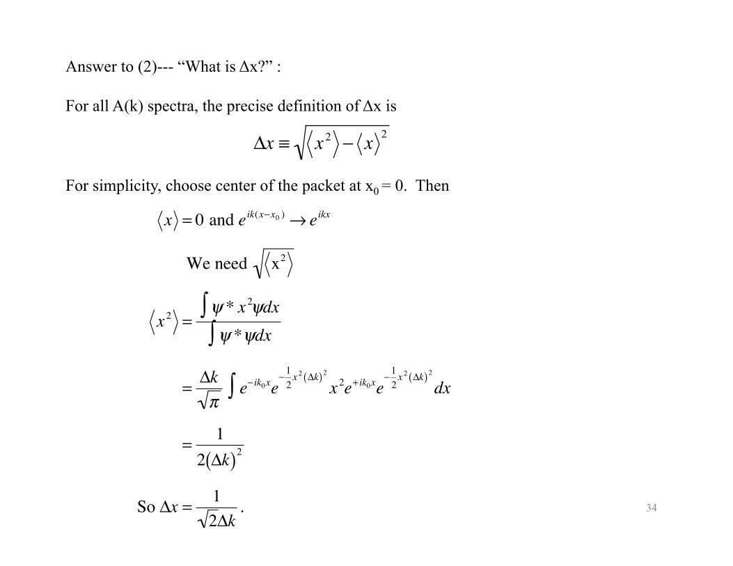
Answer to (2)--- “What is Δx?” :
For all A(k) spectra, the precise definition of Δx is
For simplicity, choose center of the packet at x0 = 0. Then
�
Δx ≡ x 2 − x 2
�
x = 0 and eik(x−x0 ) → eikx
We need x2
x 2 =ψ * x 2ψdx∫ψ *ψdx∫
= Δkπ
e− ik0xe−1
2x 2 Δk( ) 2
∫ x 2e+ ik0xe−1
2x 2 Δk( ) 2
dx
= 12 Δk( )2
So Δx = 12Δk
.
35
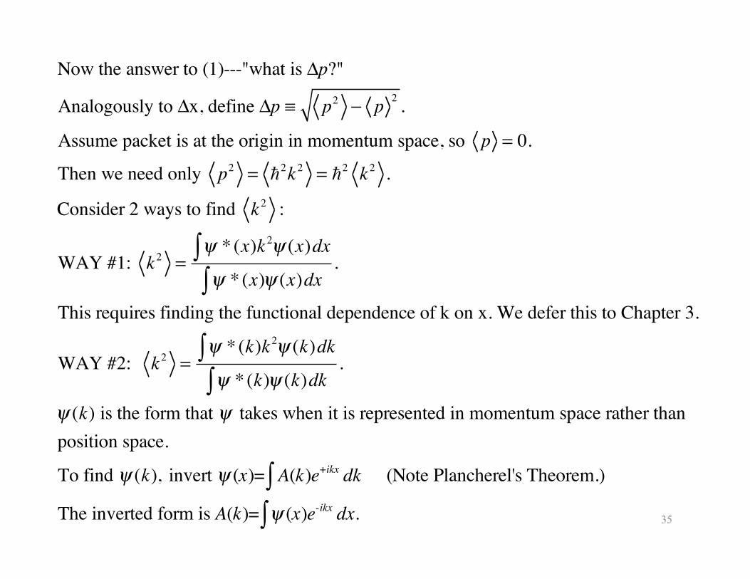
Now the answer to (1)---"what is Δp?"
Analogously to Δx, define Δp ≡ p2 − p 2 .
Assume packet is at the origin in momentum space, so p = 0.
Then we need only p2 = 2k2 = 2 k2 .
Consider 2 ways to find k2 :
WAY #1: k2 =ψ * (x)k2ψ (x)dx∫ψ * (x)ψ (x)dx∫
.
This requires finding the functional dependence of k on x. We defer this to Chapter 3.
WAY #2: k2 =ψ * (k)k2ψ (k)dk∫ψ * (k)ψ (k)dk∫
.
ψ (k) is the form that ψ takes when it is represented in momentum space rather thanposition space.
To find ψ (k), invert ψ (x)= A(k)e+ikx dk∫ (Note Plancherel's Theorem.)
The inverted form is A(k)= ψ (x)e-ikx dx.∫
36
So A(k) IS ψ (k), the k-dependent form of ψ .
So we need k2 =A*(k)k2A(k)dk
−∞
+∞
∫
A * (k)A(k)dk−∞
+∞
∫=
Δk( )2
2
So p2 = 2 k2 =
2 Δk( )2
2.
Then Δp= p2 − p 2 =
2 Δk( )2
2− 0 =
Δk2
.
Combine: ΔxΔp = 12Δk
⋅Δk
2=
2 for a Gaussian amplitude distribution.
For all other amplitude distributions, the value is > 2
, so for ANY packet,
ΔxΔp ≥
2.
We will cover the alternate uncertainty principle, ΔEΔt ≥ 2
, after Chapter 6.
37
Please read Goswami Chapter 3.
Outline I. Phase velocity and group velocity II. Wave packets spread in time III. A longer look at Fourier transforms, momentum conservation, and packet dispersion. IV. Operators V. Commutators VI. Probing the meaning of the Schroedinger Equation
38
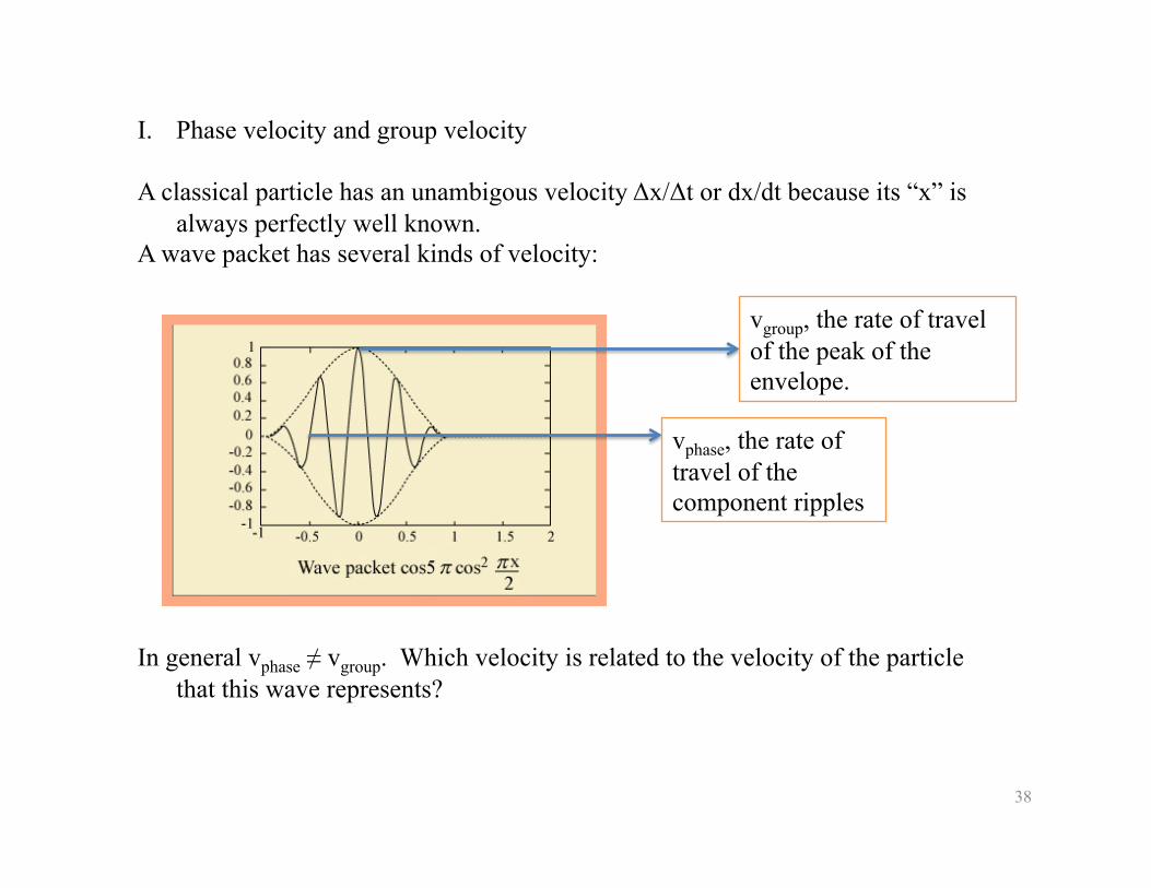
I. Phase velocity and group velocity
A classical particle has an unambigous velocity Δx/Δt or dx/dt because its “x” is always perfectly well known.
A wave packet has several kinds of velocity:
In general vphase ≠ vgroup. Which velocity is related to the velocity of the particle that this wave represents?
vgroup, the rate of travel of the peak of the envelope.
vphase, the rate of travel of the component ripples
39
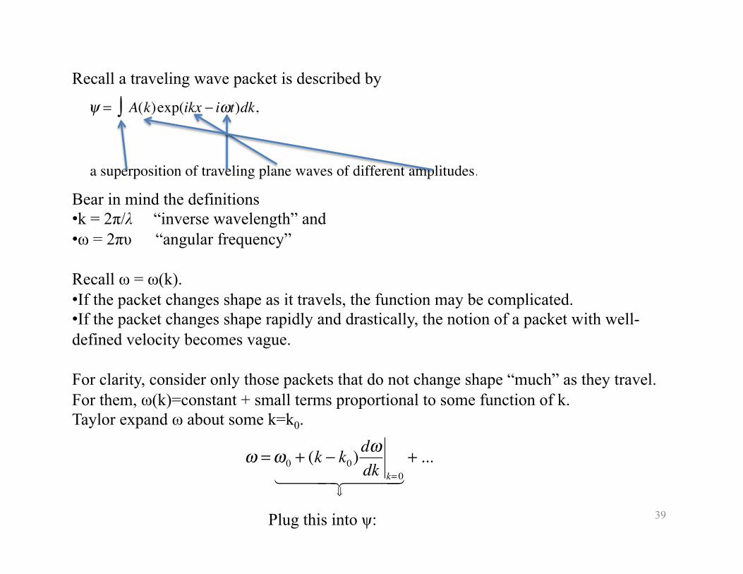
Recall a traveling wave packet is described by
Bear in mind the definitions • k = 2π/λ “inverse wavelength” and • ω = 2πυ “angular frequency”
Recall ω = ω(k). • If the packet changes shape as it travels, the function may be complicated. • If the packet changes shape rapidly and drastically, the notion of a packet with well-defined velocity becomes vague.
For clarity, consider only those packets that do not change shape “much” as they travel. For them, ω(k)=constant + small terms proportional to some function of k. Taylor expand ω about some k=k0.
Plug this into ψ:
�
ψ = A(k)exp(ikx − iωt)dk∫ ,
a superposition of traveling plane waves of different amplitudes.
�
ω = ω0 + (k − k0)dωdk k= 0
⇓
+ ...
40
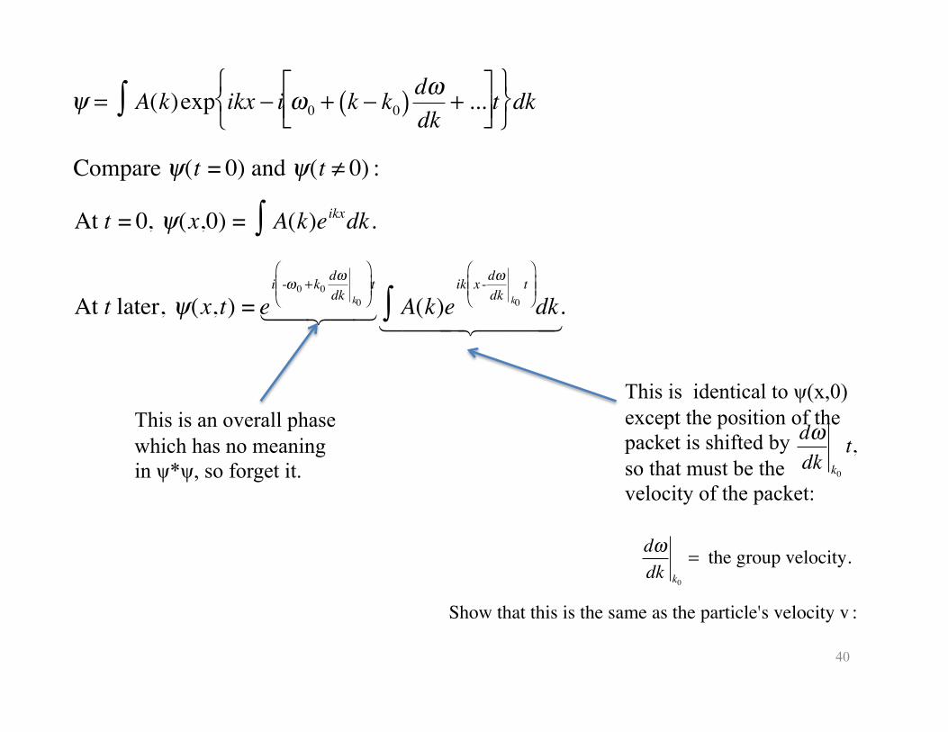
�
ψ = A(k)exp ikx − i ω0 + k − k0( ) dωdk
+ ...⎡ ⎣ ⎢
⎤ ⎦ ⎥ t
⎧ ⎨ ⎩
⎫ ⎬ ⎭ dk∫
Compare ψ(t = 0) and ψ(t ≠ 0) :
At t = 0, ψ(x,0) = A(k)eikxdk.∫
At t later, ψ(x, t) = ei -ω0 +k0
dωdk k0
⎛
⎝ ⎜ ⎜
⎞
⎠ ⎟ ⎟ t
A(k)eik x -dω
dk k0
t⎛
⎝ ⎜ ⎜
⎞
⎠ ⎟ ⎟ dk.∫
This is an overall phase which has no meaning in ψ*ψ, so forget it.
This is identical to ψ(x,0) except the position of the packet is shifted by so that must be the velocity of the packet:
�
dωdk k0
t,
�
dωdk k0
= the group velocity.
Show that this is the same as the particle's velocity v :
41
�
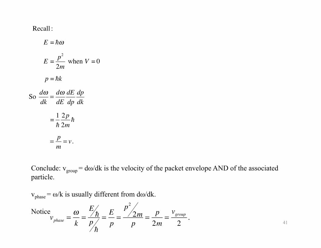
Recall :
E = ω
E = p2
2m when V = 0
p = k
So dωdk
= dωdE
dEdp
dpdk
= 1
2p2m
= pm
= v.
Conclude: vgroup = dω/dk is the velocity of the packet envelope AND of the associated particle.
vphase = ω/k is usually different from dω/dk.
Notice
vphase =ωk=E
p
=Ep=p22mp
=p2m
=vgroup2.
42
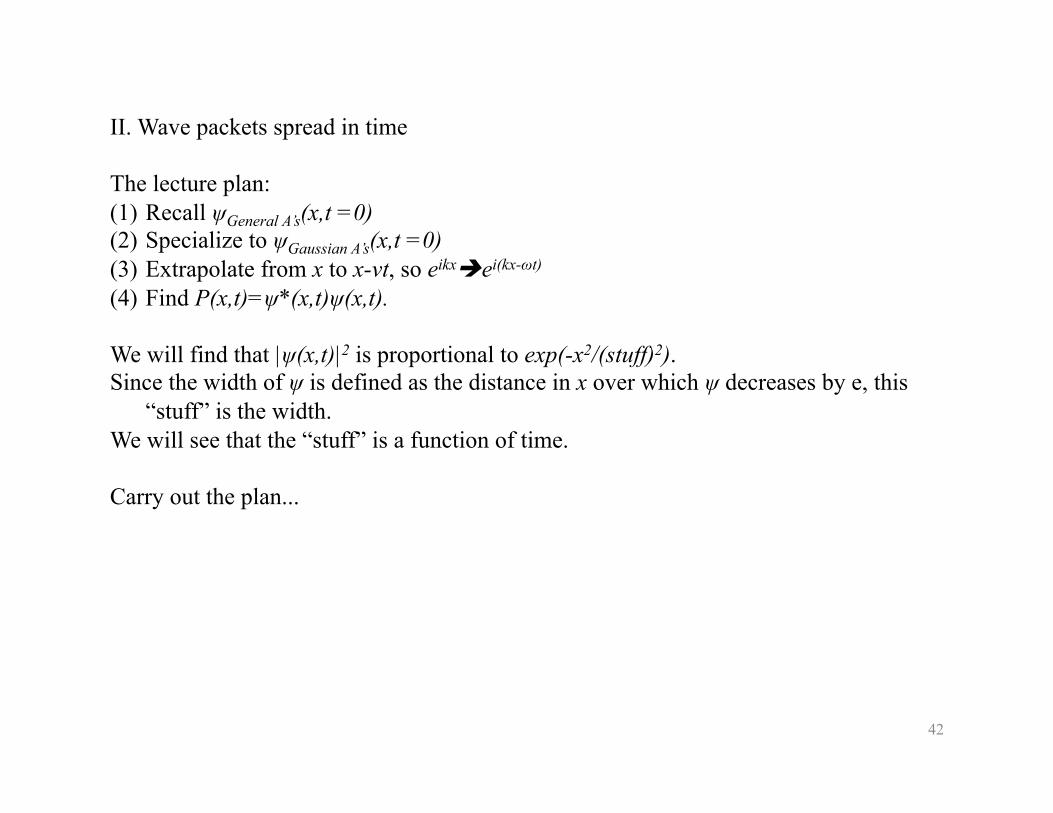
II. Wave packets spread in time
The lecture plan: (1) Recall ψGeneral A’s(x,t =0) (2) Specialize to ψGaussian A’s(x,t =0) (3) Extrapolate from x to x-vt, so eikxei(kx-ωt)
(4) Find P(x,t)=ψ*(x,t)ψ(x,t).
We will find that |ψ(x,t)|2 is proportional to exp(-x2/(stuff)2). Since the width of ψ is defined as the distance in x over which ψ decreases by e, this
“stuff” is the width. We will see that the “stuff” is a function of time.
Carry out the plan...
43
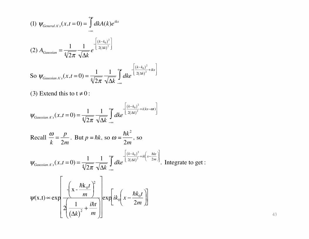
�
(1) ψGeneral A 's(x,t = 0) = dkA(k)eikx−∞
+∞
∫
(2) AGaussian = 12π4
1Δk
e−
k−k0( ) 2
2 Δk( ) 2
⎡
⎣ ⎢ ⎢
⎤
⎦ ⎥ ⎥
So ψGaussian A 's(x,t = 0) = 12π4
1Δk
dk−∞
+∞
∫ e−
k−k0( ) 2
2 Δk( ) 2 + ikx⎡
⎣ ⎢ ⎢
⎤
⎦ ⎥ ⎥
(3) Extend this to t ≠ 0 :
ψGaussian A 's(x,t = 0) = 12π4
1Δk
dk−∞
+∞
∫ e−
k−k0( ) 2
2 Δk( ) 2 + i(kx−ωt )⎡
⎣ ⎢ ⎢
⎤
⎦ ⎥ ⎥
Recall ωk
= p2m
. But p = k, so ω = k2
2m, so
ψGaussian A 's(x,t = 0) = 12π4
1Δk
dk−∞
+∞
∫ e−
k−k0( ) 2
2 Δk( ) 2 + ik x− kt2m
⎛ ⎝ ⎜
⎞ ⎠ ⎟
⎡
⎣ ⎢ ⎢
⎤
⎦ ⎥ ⎥ . Integrate to get :
ψ(x,t)∝exp- x - k0t
m⎛ ⎝ ⎜
⎞ ⎠ ⎟
2
2 1Δk( )2 + it
m
⎛
⎝ ⎜ ⎜
⎞
⎠ ⎟ ⎟
⎡
⎣
⎢ ⎢ ⎢ ⎢ ⎢
⎤
⎦
⎥ ⎥ ⎥ ⎥ ⎥
exp ik0 x − k0t2m
⎛ ⎝ ⎜
⎞ ⎠ ⎟
⎡ ⎣ ⎢
⎤ ⎦ ⎥
44
(4) ψ *ψ ∝ exp- x- k0t
m⎛⎝⎜
⎞⎠⎟
2
2 1Δk( )2 + it
m⎛
⎝⎜⎞
⎠⎟
⎡
⎣
⎢⎢⎢⎢⎢
⎤
⎦
⎥⎥⎥⎥⎥
exp- x- k0t
m⎛⎝⎜
⎞⎠⎟
2
2 1Δk( )2 − it
m⎛
⎝⎜⎞
⎠⎟
⎡
⎣
⎢⎢⎢⎢⎢
⎤
⎦
⎥⎥⎥⎥⎥
∝ exp −1Δk( )2
x − k0tm
⎛⎝⎜
⎞⎠⎟
1Δk( )4 +
2t 2
m2
⎡
⎣
⎢⎢⎢⎢
⎤
⎦
⎥⎥⎥⎥
⎧
⎨⎪⎪
⎩⎪⎪
⎫
⎬⎪⎪
⎭⎪⎪
.
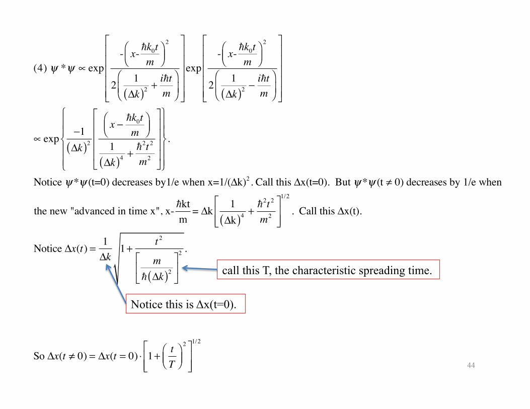
Notice ψ*ψ (t=0) decreases by1/e when x=1/(Δk)2. Call this Δx(t=0). But ψ*ψ (t ≠ 0) decreases by 1/e when
the new "advanced in time x", x- ktm
= Δk 1Δk( )4 +
2t 2
m2
⎡
⎣⎢⎢
⎤
⎦⎥⎥
1/2
. Call this Δx(t).
Notice Δx(t) = 1Δk
1+ t 2
m Δk( )2
⎡
⎣⎢
⎤
⎦⎥
2 .
So Δx(t ≠ 0) = Δx(t = 0) ⋅ 1+ tT
⎛⎝⎜
⎞⎠⎟
2⎡
⎣⎢⎢
⎤
⎦⎥⎥
1/2
call this T, the characteristic spreading time.
Notice this is Δx(t=0).
45
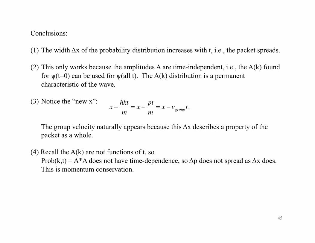
Conclusions:
(1) The width Δx of the probability distribution increases with t, i.e., the packet spreads.
(2) This only works because the amplitudes A are time-independent, i.e., the A(k) found for ψ(t=0) can be used for ψ(all t). The A(k) distribution is a permanent characteristic of the wave.
(3) Notice the “new x”:
The group velocity naturally appears because this Δx describes a property of the packet as a whole.
(4) Recall the A(k) are not functions of t, so Prob(k,t) = A*A does not have time-dependence, so Δp does not spread as Δx does. This is momentum conservation.
�
x − ktm
= x − ptm
= x − vgroup t.
46
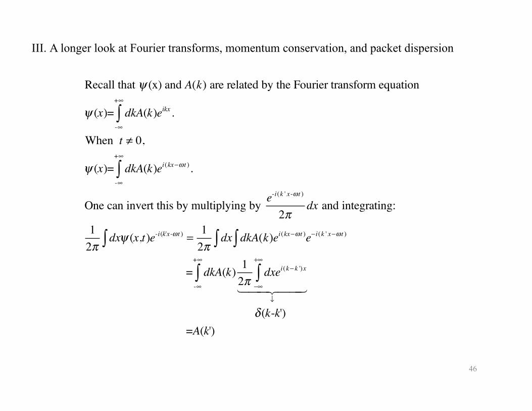
III. A longer look at Fourier transforms, momentum conservation, and packet dispersion
Recall that ψ (x) and A(k) are related by the Fourier transform equation
ψ (x)= dkA(k)eikx .-∞
+∞
∫When t ≠ 0,
ψ (x)= dkA(k)ei(kx−ω t ).-∞
+∞
∫
One can invert this by multiplying by e-i(k ' x-ω t )
2πdx and integrating:
12π
dxψ (x,t)e-i(k'x-ω t ) =1
2πdx dkA(k)ei(kx−ω t )e− i(k ' x−ω t )∫∫∫
= dkA(k) 12π
dxei(k− k ')x
−∞
+∞
∫↓
-∞
+∞
∫
δ (k-k') =A(k')
47
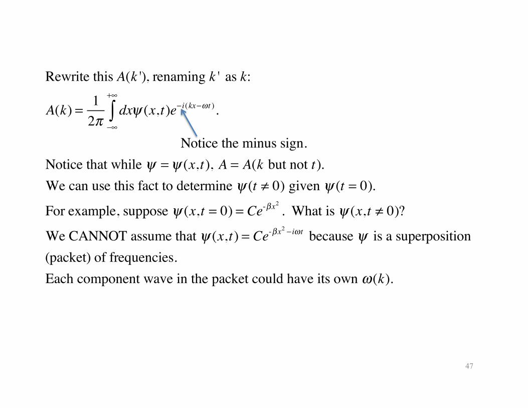
Rewrite this A(k '), renaming k ' as k:
A(k) = 12π
dxψ (x,t)e− i(kx−ω t ).−∞
+∞
∫ Notice the minus sign.Notice that while ψ =ψ (x,t), A = A(k but not t).We can use this fact to determine ψ (t ≠ 0) given ψ (t = 0).
For example, suppose ψ (x,t = 0) = Ce-βx2
. What is ψ (x,t ≠ 0)?
We CANNOT assume that ψ (x,t) = Ce-βx2 − iω t because ψ is a superposition (packet) of frequencies.Each component wave in the packet could have its own ω (k).
48
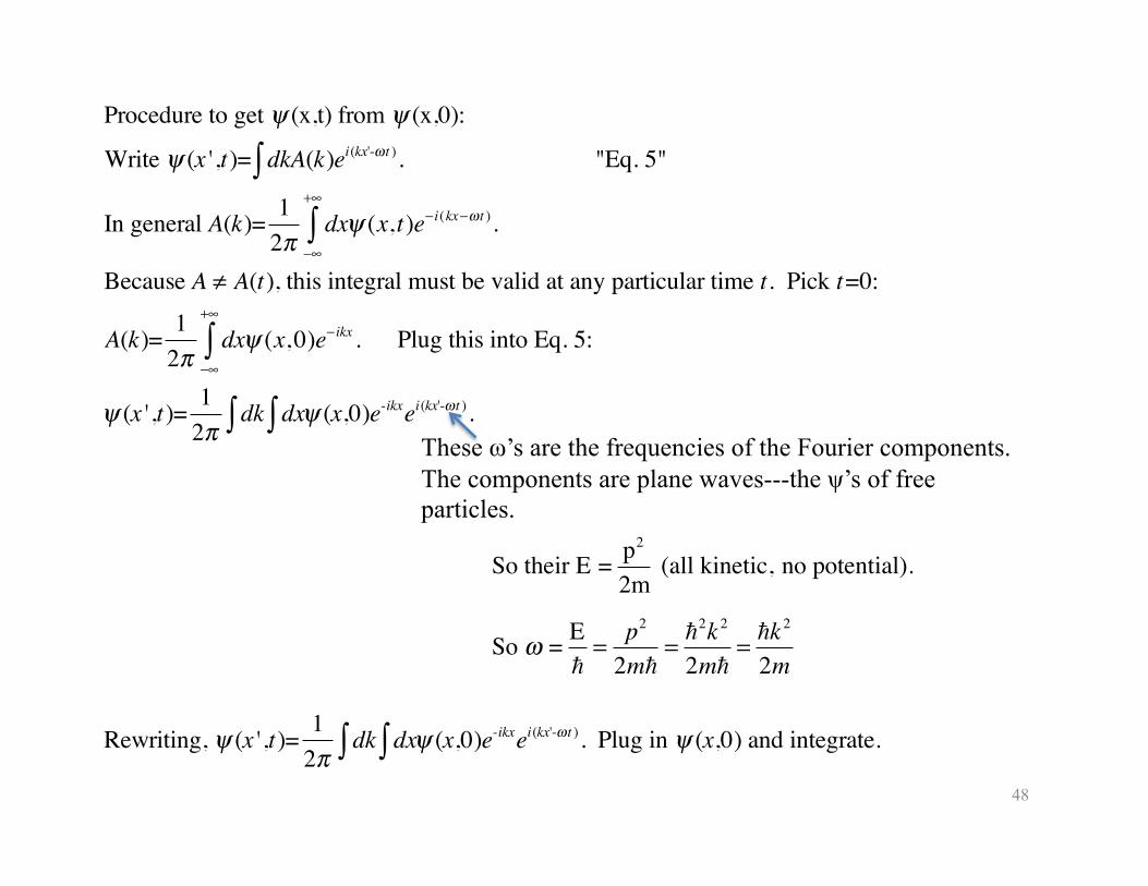
Procedure to get ψ (x,t) from ψ (x,0):
Write ψ (x ',t)= dkA(k)ei(kx'-ω t ).∫ "Eq. 5"
In general A(k)= 12π
dxψ (x,t)e− i(kx−ω t ).−∞
+∞
∫Because A ≠ A(t), this integral must be valid at any particular time t. Pick t=0:
A(k)= 12π
dxψ (x,0)e− ikx .−∞
+∞
∫ Plug this into Eq. 5:
ψ (x ',t)= 12π
dk dx∫ ψ (x,0)e-ikxei(kx'-ω t ).∫
Rewriting, ψ (x ',t)= 12π
dk dx∫ ψ (x,0)e-ikxei(kx'-ω t ).∫ Plug in ψ (x,0) and integrate.
These ω’s are the frequencies of the Fourier components. The components are plane waves---the ψ’s of free particles.
�
So their E = p2
2m (all kinetic, no potential).
So ω = E
= p2
2m=
2k 2
2m= k
2
2m
49
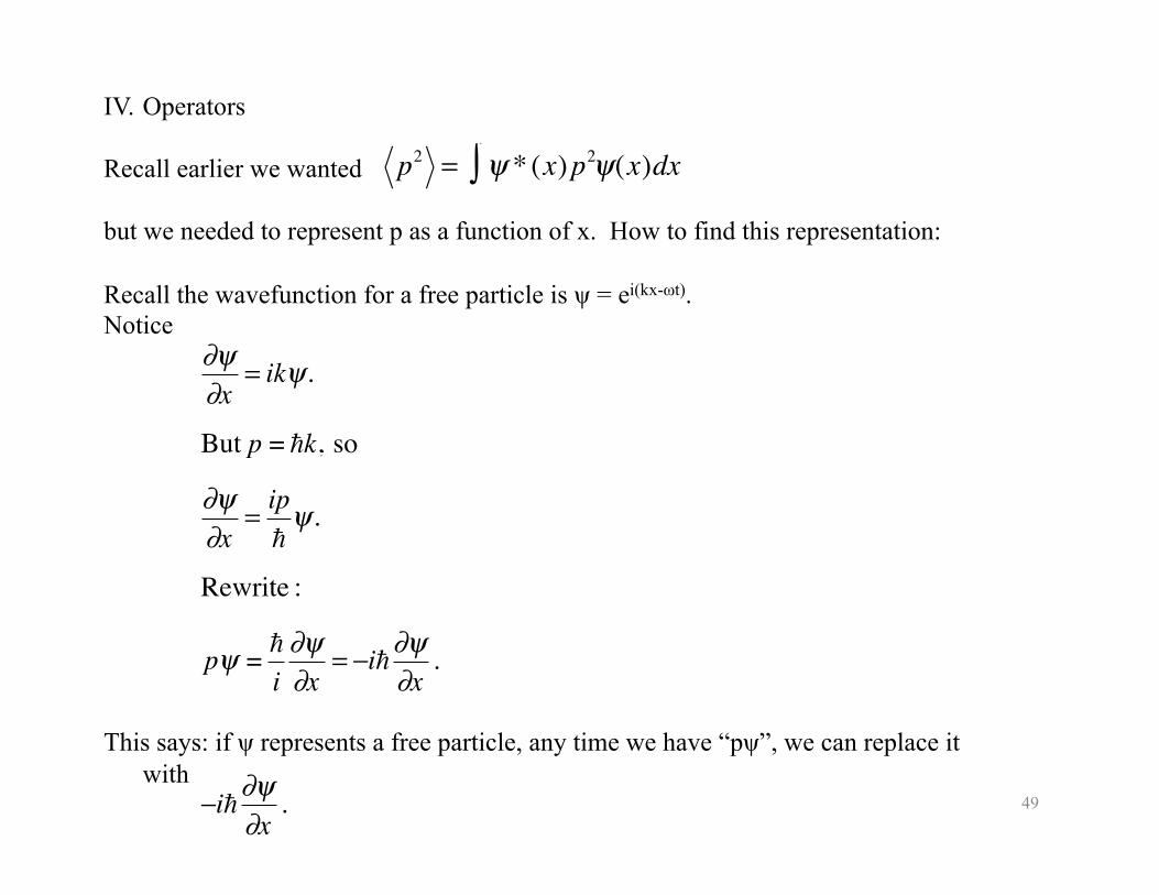
IV. Operators
Recall earlier we wanted
but we needed to represent p as a function of x. How to find this representation:
Recall the wavefunction for a free particle is ψ = ei(kx-ωt). Notice
This says: if ψ represents a free particle, any time we have “pψ”, we can replace it with
�
p2 = ψ * (x)p2ψ(x)dx∫
�
∂ψ∂x
= ikψ.
But p = k, so
∂ψ∂x
= ipψ.
Rewrite :
pψ = i∂ψ∂x
= −i∂ψ∂x
.
−i∂ψ∂x
.
50
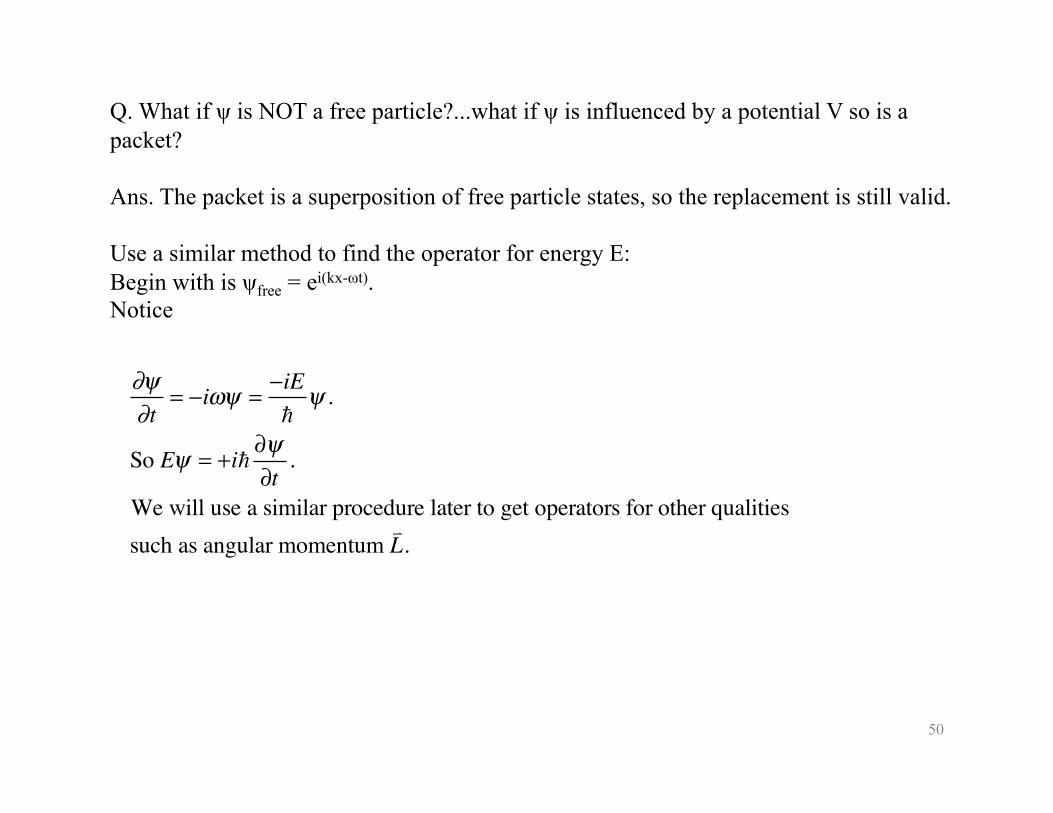
Q. What if ψ is NOT a free particle?...what if ψ is influenced by a potential V so is a packet?
Ans. The packet is a superposition of free particle states, so the replacement is still valid.
Use a similar method to find the operator for energy E: Begin with is ψfree = ei(kx-ωt). Notice
∂ψ∂t
= −iωψ =−iE
ψ .
So Eψ = +i∂ψ∂t
.
We will use a similar procedure later to get operators for other qualities such as angular momentum
L.
51
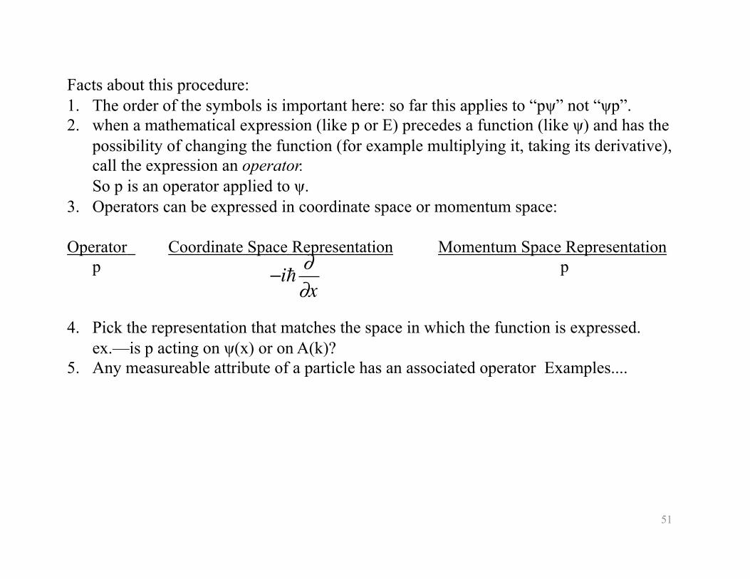
Facts about this procedure: 1. The order of the symbols is important here: so far this applies to “pψ” not “ψp”. 2. when a mathematical expression (like p or E) precedes a function (like ψ) and has the
possibility of changing the function (for example multiplying it, taking its derivative), call the expression an operator. So p is an operator applied to ψ.
3. Operators can be expressed in coordinate space or momentum space:
Operator Coordinate Space Representation Momentum Space Representation p p
4. Pick the representation that matches the space in which the function is expressed. ex.—is p acting on ψ(x) or on A(k)?
5. Any measureable attribute of a particle has an associated operator Examples....
�
−i ∂∂x
52
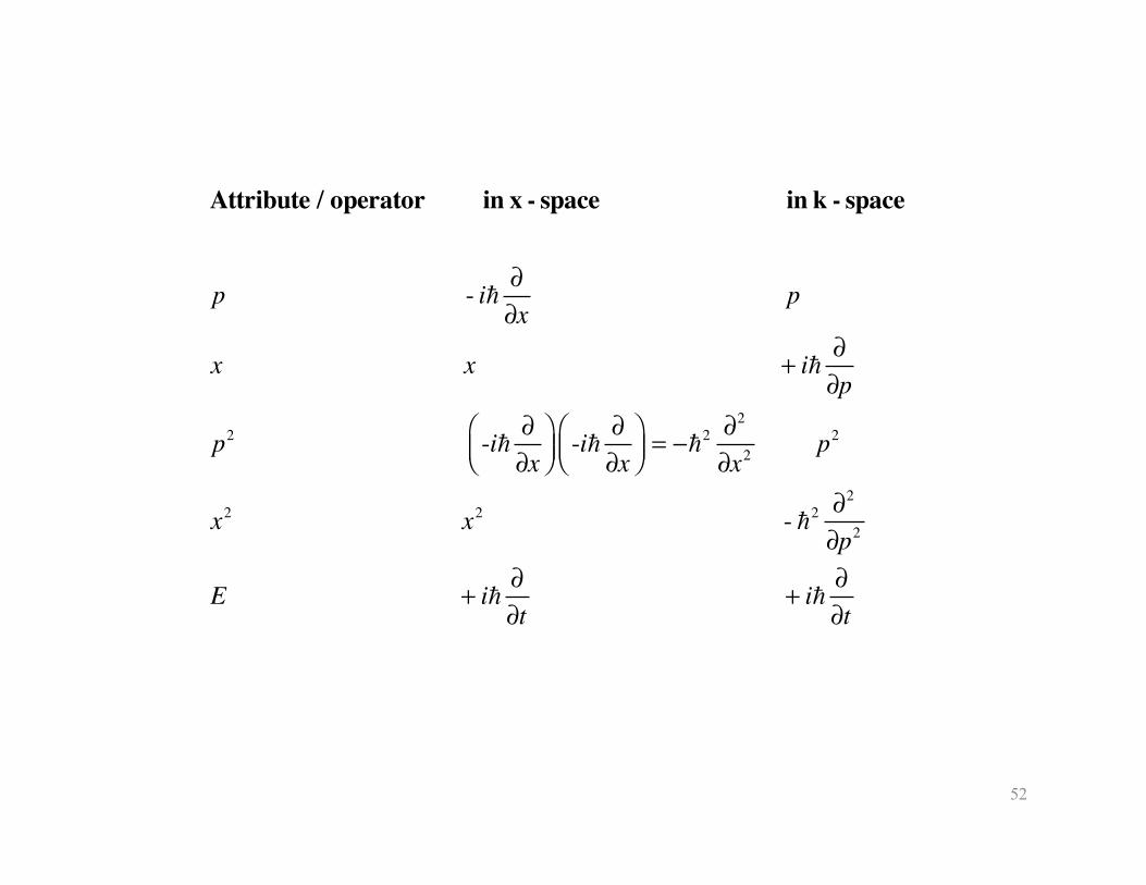
Attribute / operator in x - space in k - space
p - i ∂∂x
p
x x + i ∂∂p
p2 -i ∂∂x
⎛⎝⎜
⎞⎠⎟
-i ∂∂x
⎛⎝⎜
⎞⎠⎟= −2 ∂2
∂x2 p2
x2 x2 - 2 ∂2
∂p2
E + i ∂∂t
+ i ∂∂t
53
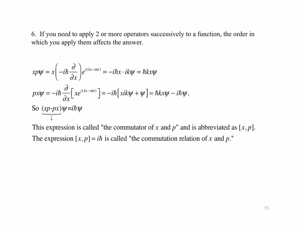
6. If you need to apply 2 or more operators successively to a function, the order in which you apply them affects the answer.
xpψ = x −i∂∂x
⎛⎝⎜
⎞⎠⎟ei(kx−ω t ) = −ix ⋅ ikψ = kxψ
pxψ = −i∂∂x
xei(kx−ω t )⎡⎣ ⎤⎦ = −i xikψ +ψ[ ] = kxψ − iψ .
So (xp-px)↓
ψ =iψ
This expression is called "the commutator of x and p" and is abbreviated as [x, p].The expression [x, p] = i is called "the commutation relation of x and p."
54
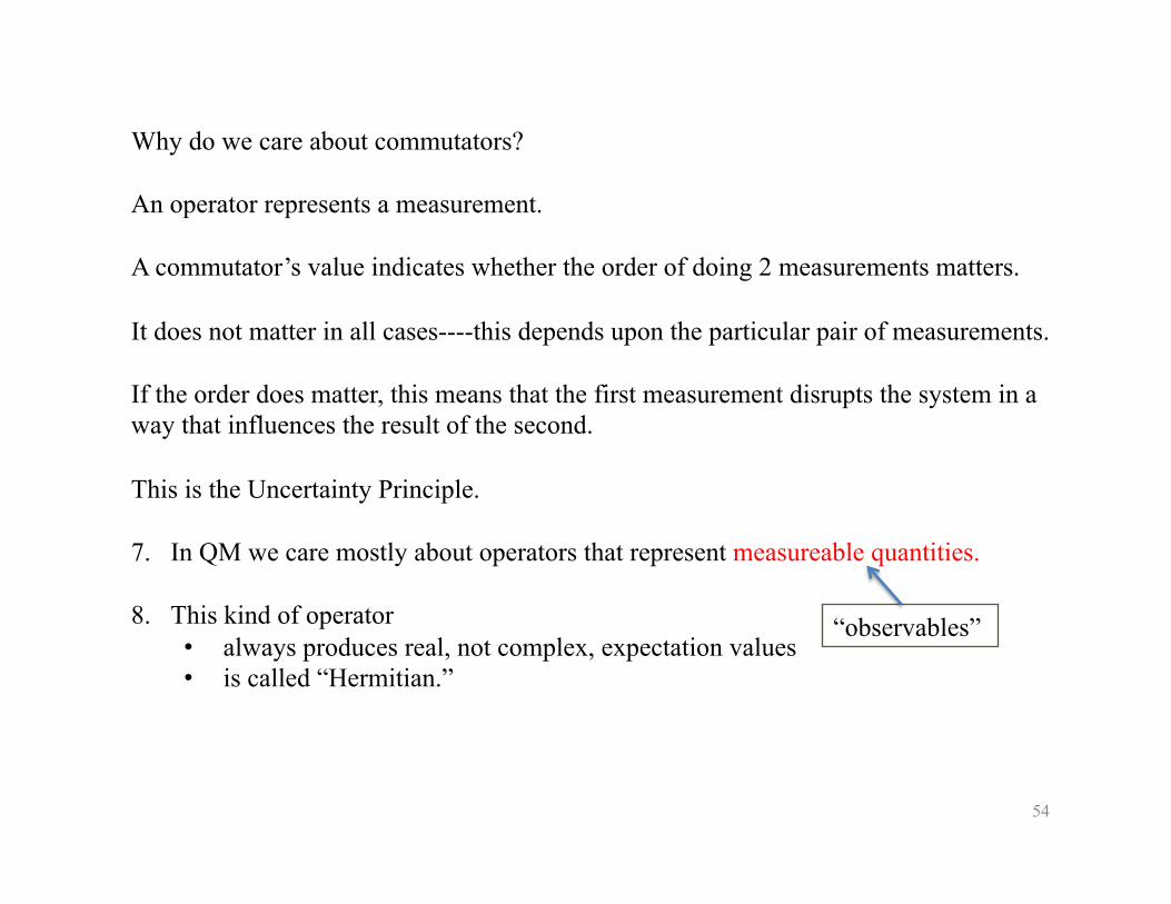
Why do we care about commutators?
An operator represents a measurement.
A commutator’s value indicates whether the order of doing 2 measurements matters.
It does not matter in all cases----this depends upon the particular pair of measurements.
If the order does matter, this means that the first measurement disrupts the system in a way that influences the result of the second.
This is the Uncertainty Principle.
7. In QM we care mostly about operators that represent measureable quantities.
8. This kind of operator • always produces real, not complex, expectation values • is called “Hermitian.”
“observables”
55
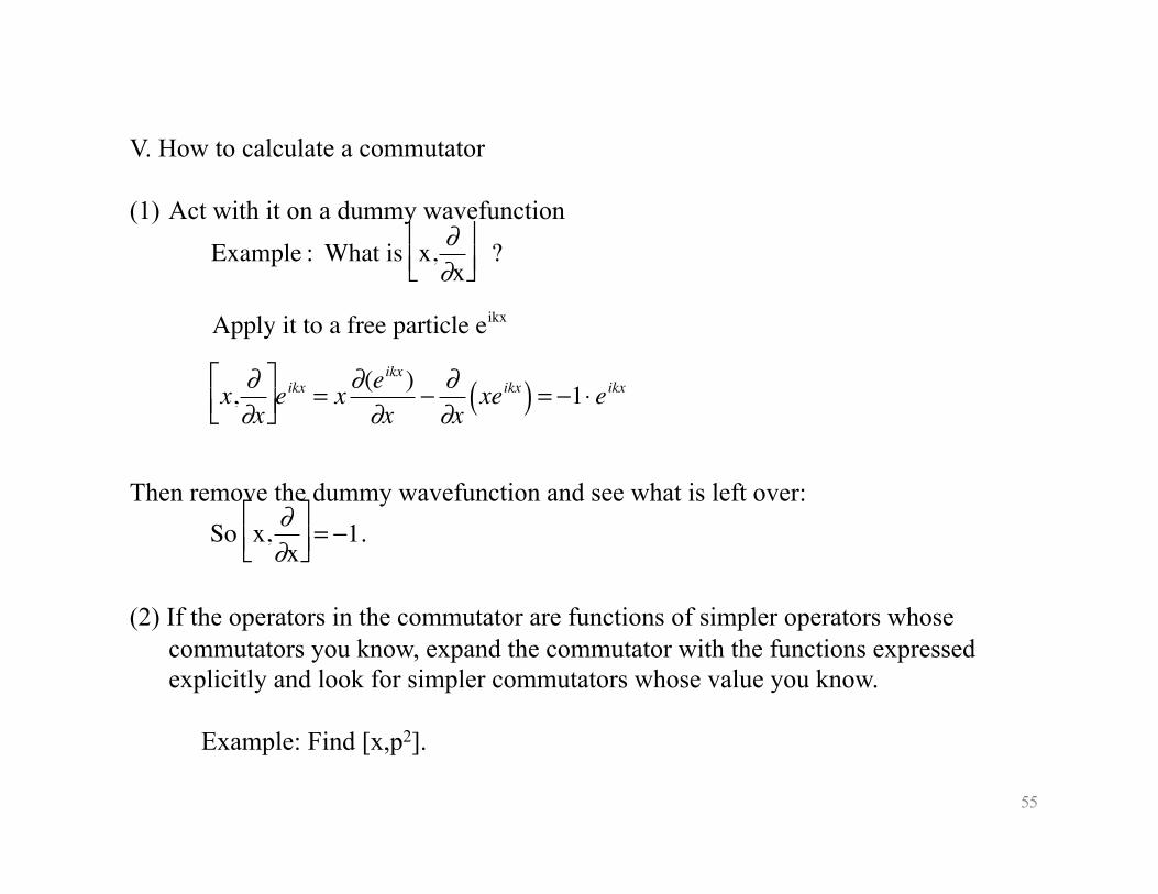
V. How to calculate a commutator
(1) Act with it on a dummy wavefunction
Then remove the dummy wavefunction and see what is left over:
(2) If the operators in the commutator are functions of simpler operators whose commutators you know, expand the commutator with the functions expressed explicitly and look for simpler commutators whose value you know.
Example: Find [x,p2].
�
Example : What is x, ∂∂x
⎡ ⎣ ⎢
⎤ ⎦ ⎥ ?
Apply it to a free particle eikx
x, ∂∂x
⎡ ⎣ ⎢
⎤ ⎦ ⎥ e
ikx = x ∂(eikx )∂x
− ∂∂x
xeikx( ) = −1⋅ eikx
So x, ∂∂x
⎡ ⎣ ⎢
⎤ ⎦ ⎥ = −1.
56
�
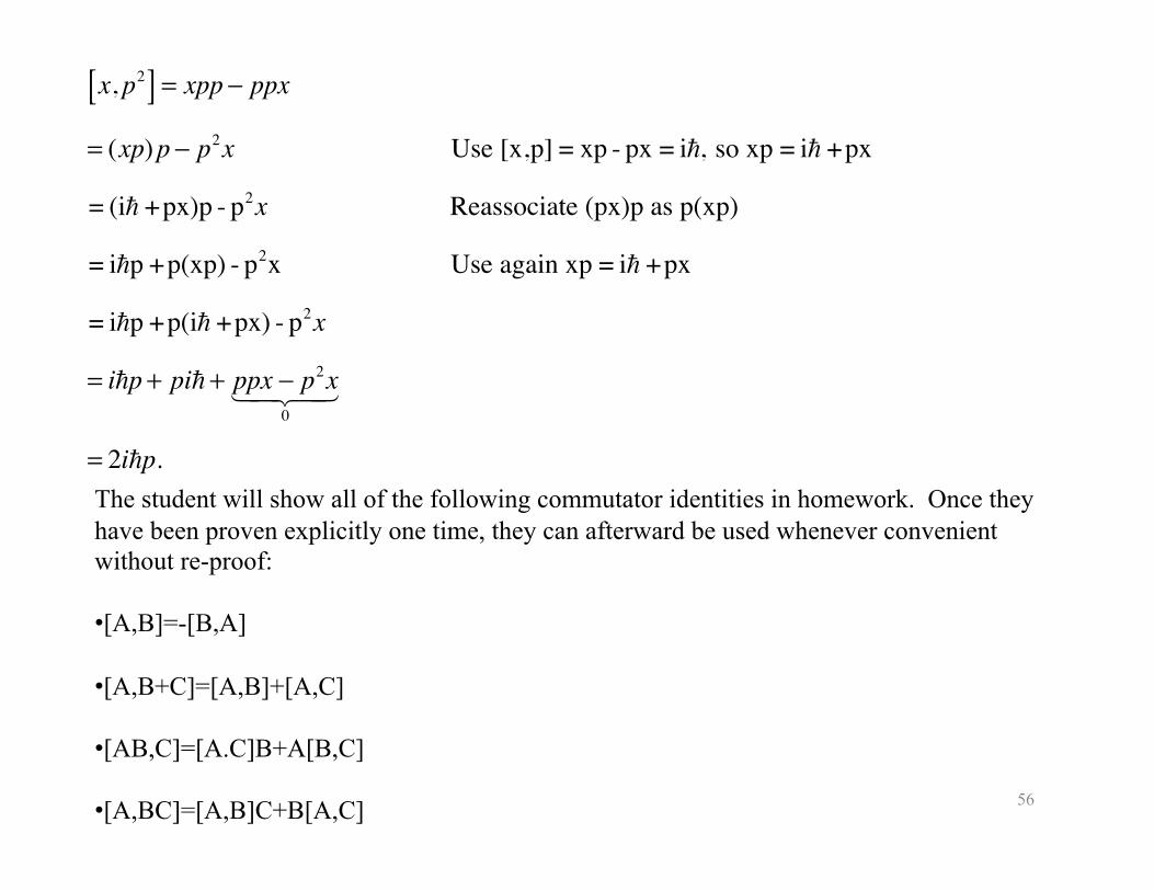
x, p2[ ] = xpp − ppx
= (xp)p − p2x Use [x,p] = xp - px = i, so xp = i +px
= (i +px)p - p2x Reassociate (px)p as p(xp)
= ip +p(xp) - p2x Use again xp = i +px
= ip +p(i +px) - p2x
= ip + pi + ppx − p2x0
= 2ip.The student will show all of the following commutator identities in homework. Once they have been proven explicitly one time, they can afterward be used whenever convenient without re-proof:
• [A,B]=-[B,A]
• [A,B+C]=[A,B]+[A,C]
• [AB,C]=[A.C]B+A[B,C]
• [A,BC]=[A,B]C+B[A,C]
57
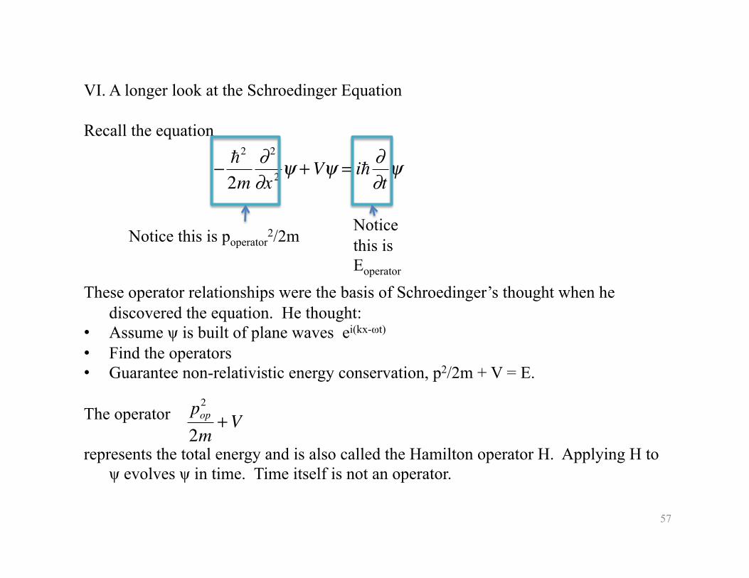
VI. A longer look at the Schroedinger Equation
Recall the equation
These operator relationships were the basis of Schroedinger’s thought when he discovered the equation. He thought:
• Assume ψ is built of plane waves ei(kx-ωt)
• Find the operators • Guarantee non-relativistic energy conservation, p2/2m + V = E.
The operator
represents the total energy and is also called the Hamilton operator H. Applying H to ψ evolves ψ in time. Time itself is not an operator.
�
− 2
2m∂ 2
∂x 2ψ +Vψ = i ∂
∂tψ
Notice this is poperator2/2m Notice
this is Eoperator
�
pop2
2m+V
58
Please read Goswami Chapter 4
Outline I. How to solve the Schroedinger Equation II. Why do we concentrate on ψ’s that are separable? III. Why E is real if ψ=u(x)T(t)
59
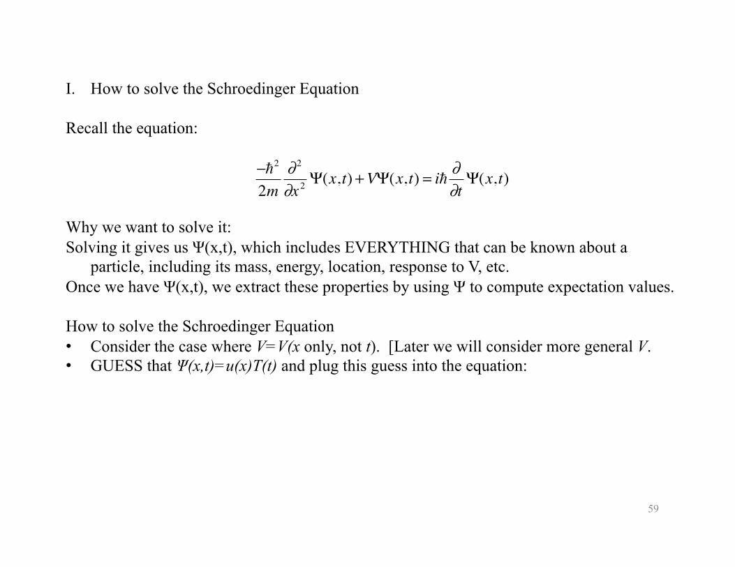
I. How to solve the Schroedinger Equation
Recall the equation:
Why we want to solve it: Solving it gives us Ψ(x,t), which includes EVERYTHING that can be known about a
particle, including its mass, energy, location, response to V, etc. Once we have Ψ(x,t), we extract these properties by using Ψ to compute expectation values.
How to solve the Schroedinger Equation • Consider the case where V=V(x only, not t). [Later we will consider more general V. • GUESS that Ψ(x,t)=u(x)T(t) and plug this guess into the equation:
�
−2
2m∂ 2
∂x 2Ψ(x,t) +VΨ(x, t) = i ∂
∂tΨ(x, t)
60
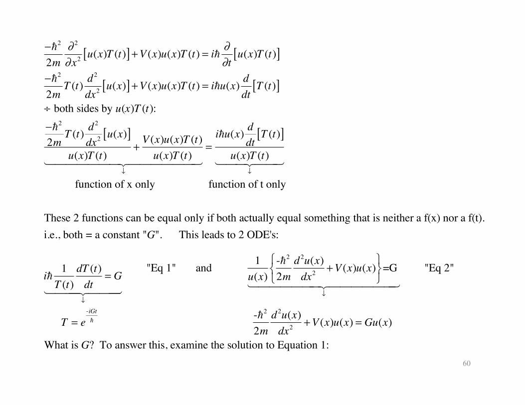
−2
2m∂ 2
∂x2 u(x)T (t)[ ] +V (x)u(x)T (t) = i ∂∂t
u(x)T (t)[ ]−2
2mT (t) d
2
dx2 u(x)[ ] +V (x)u(x)T (t) = iu(x) ddt
T (t)[ ]÷ both sides by u(x)T (t):−2
2mT (t) d
2
dx2 u(x)[ ]u(x)T (t)
+V (x)u(x)T (t)u(x)T (t)
↓
=iu(x) d
dtT (t)[ ]
u(x)T (t)↓
function of x only function of t only
These 2 functions can be equal only if both actually equal something that is neither a f(x) nor a f(t).i.e., both = a constant "G". This leads to 2 ODE's:
i1
T (t)dT (t)dt
= G
↓
"Eq 1" and 1u(x)
-2
2md 2u(x)dx2 +V (x)u(x)
⎧⎨⎩
⎫⎬⎭
=G
↓
"Eq 2"
T = e-iGt -2
2md 2u(x)dx2 +V (x)u(x) = Gu(x)
What is G? To answer this, examine the solution to Equation 1:
61
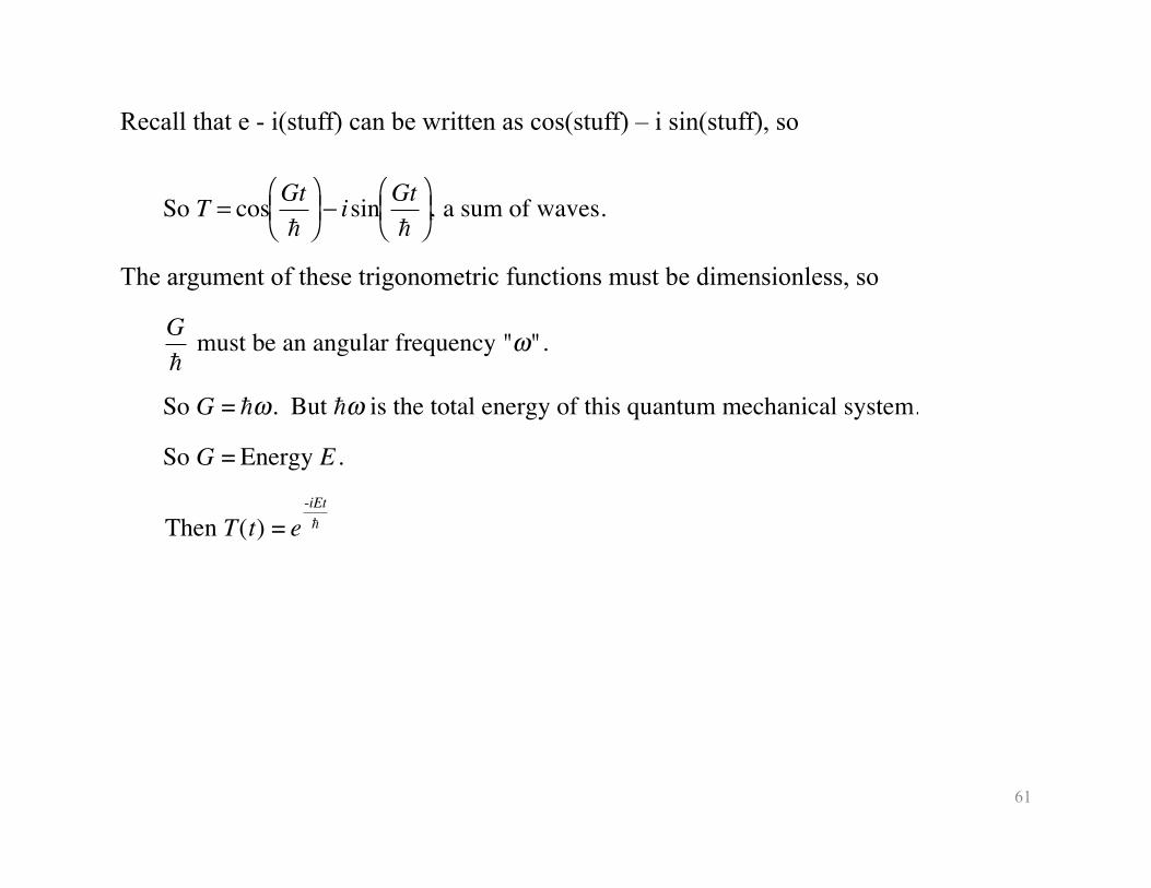
Recall that e - i(stuff) can be written as cos(stuff) – i sin(stuff), so
The argument of these trigonometric functions must be dimensionless, so
�
So T = cos Gt
⎛ ⎝ ⎜
⎞ ⎠ ⎟ − isin Gt
⎛ ⎝ ⎜
⎞ ⎠ ⎟ , a sum of waves.
G
must be an angular frequency "ω".
So G = ω. But ω is the total energy of this quantum mechanical system.
So G = Energy E .
Then T(t) = e-iEt
62
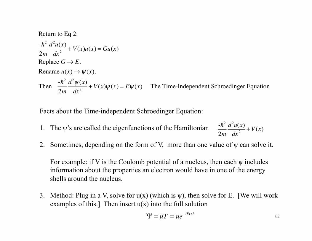
Return to Eq 2:-2
2md 2u(x)dx2 +V (x)u(x) = Gu(x)
Replace G→ E.Rename u(x)→ψ (x).
Then -2
2md 2ψ (x)dx2 +V (x)ψ (x) = Eψ (x) The Time-Independent Schroedinger Equation
Facts about the Time-independent Schroedinger Equation:
1. The ψ’s are called the eigenfunctions of the Hamiltonian
2. Sometimes, depending on the form of V, more than one value of ψ can solve it.
For example: if V is the Coulomb potential of a nucleus, then each ψ includes information about the properties an electron would have in one of the energy shells around the nucleus.
3. Method: Plug in a V, solve for u(x) (which is ψ), then solve for E. [We will work examples of this.] Then insert u(x) into the full solution
�
-2
2md2u(x)dx 2
+V (x)
Ψ = uT = ue− iEt /
63
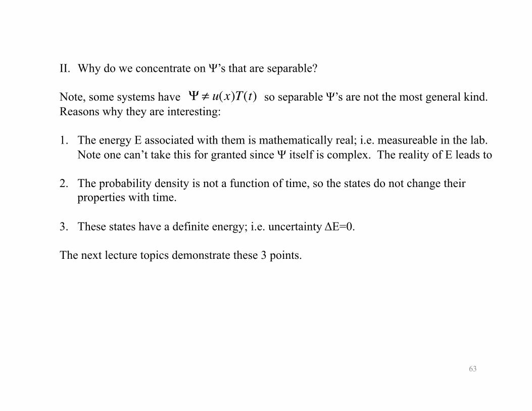
II. Why do we concentrate on Ψ’s that are separable?
Note, some systems have so separable Ψ’s are not the most general kind. Reasons why they are interesting:
1. The energy E associated with them is mathematically real; i.e. measureable in the lab. Note one can’t take this for granted since Ψ itself is complex. The reality of E leads to
2. The probability density is not a function of time, so the states do not change their properties with time.
3. These states have a definite energy; i.e. uncertainty ΔE=0.
The next lecture topics demonstrate these 3 points.
�
Ψ ≠ u(x)T(t)
64
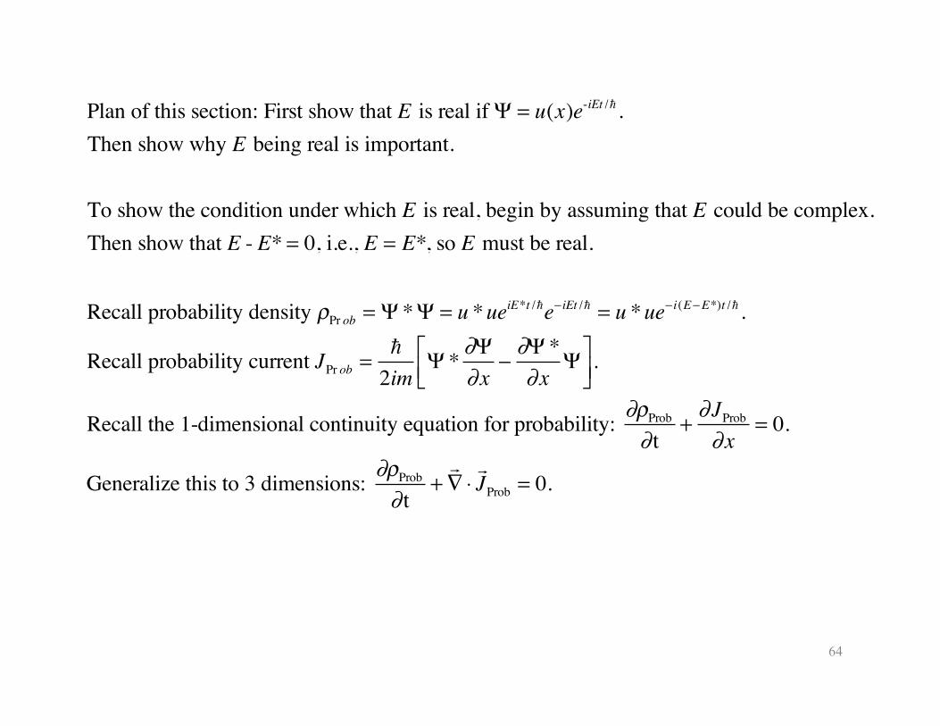
Plan of this section: First show that E is real if Ψ = u(x)e-iEt / . Then show why E being real is important.
To show the condition under which E is real, begin by assuming that E could be complex.Then show that E - E* = 0, i.e., E = E*, so E must be real.
Recall probability density ρPr ob = Ψ *Ψ = u *ueiE*t /e− iEt / = u *ue− i(E−E*)t / .
Recall probability current JPr ob =
2imΨ * ∂Ψ
∂x−∂Ψ *∂x
Ψ⎡⎣⎢
⎤⎦⎥.
Recall the 1-dimensional continuity equation for probability: ∂ρProb
∂ t+∂JProb
∂x= 0.
Generalize this to 3 dimensions: ∂ρProb
∂ t+∇ ⋅JProb = 0.
65
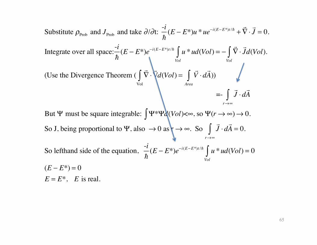
Substitute ρProb and JProb and take ∂ /∂ t: -i
(E − E*)u *ue− i(E−E*)t / +∇ ⋅J = 0.
Integrate over all space:-i
(E − E*)e− i(E−E*)t / u *uVol∫ d(Vol) = −
∇ ⋅J
Vol∫ d(Vol).
(Use the Divergence Theorem (∇ ⋅V
Vol∫ d(Vol) =
V ⋅dA
Area∫ ))
=-J ⋅dA
r→∞∫
But Ψ must be square integrable: Ψ*Ψd(Vol)<∞, so Ψ(r→∞)→ 0.∫So J, being proportional to Ψ, also → 0 as r →∞. So
J ⋅dA
r→∞∫ = 0.
So lefthand side of the equation, -i
(E − E*)e− i(E−E*)t / u *uVol∫ d(Vol) = 0
(E − E*) = 0E = E*, E is real.
66
Outline
I. Stationary States II. If Ψ is a stationary state, its ΔE=0. III. Degeneracy IV. Required properties of eigenfunctions V. Solving the time-independent Schroedinger Equation when V=0$VI. Solving the time-independent Schroedinger Equation for a Barrier Potential

67
I. Stationary States
Recall that Ψ is separable as u(x)T(t), thenΨ = u(x)e-iEt / .
If E were complex (E = ER + iEI ), then we would haveΨ = u(x)e-i(ER + iEI )t / .Then Ψ*Ψ would be u *u e-2tEI /
.
i.e., Probability of locating the particle would be time-dependent.
Expectation values f (x) =Ψ * f (x)Ψdx∫Ψ *Ψdx∫
of all the properties of Ψ would involve e-2tEI / too.
But since E is real when Ψ = u(x)T (t), Probability, expectation values ≠ f (t).So once we know something about the state, it remains true for ever.These are called stationary states.
68
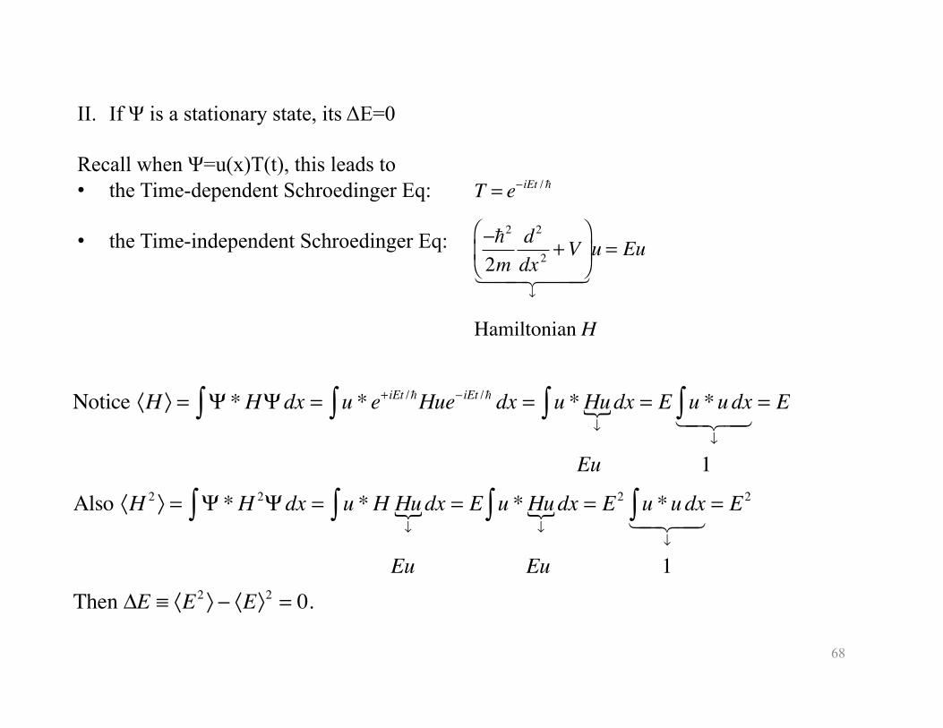
II. If Ψ is a stationary state, its ΔΕ=0
Recall when Ψ=u(x)T(t), this leads to • the Time-dependent Schroedinger Eq:
• the Time-independent Schroedinger Eq:
�
T = e−iEt /
−2
2md2
dx 2 +V⎛
⎝ ⎜
⎞
⎠ ⎟
↓
u = Eu
Hamiltonian H
Notice 〈H 〉 = Ψ *HΨdx = u * e+ iEt /Hue− iEt / dx∫∫ = u *Hu↓dx∫ = E u *udx∫
↓
= E
Eu 1
Also 〈H 2 〉 = Ψ *H 2Ψdx = u *H Hu↓dx∫∫ = E u *Hu
↓dx∫ = E2 u *udx∫
↓
= E2
Eu Eu 1Then ΔE ≡ 〈E2 〉 − 〈E〉2 = 0.
69
III. Degeneracy
If 2 states of the same system have the same energy, we call them degenerate. Example: the rightward and leftward traveling components of the free particle Ψ:
Ψ = δ cos kx ±ωt( ) ± i sin kx ±ωt( )⎡⎣ ⎤⎦ ⇒δe± i kx±ω t( )
δe+ i kx−ω t( ) : traveling rightward
δe− i kx+ω t( ) : traveling leftward
70
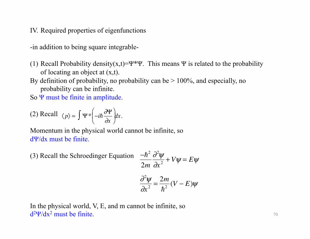
IV. Required properties of eigenfunctions
-in addition to being square integrable-
(1) Recall Probability density(x,t)=Ψ*Ψ. This means Ψ is related to the probability of locating an object at (x,t).
By definition of probability, no probability can be > 100%, and especially, no probability can be infinite.
So Ψ must be finite in amplitude.
(2) Recall
Momentum in the physical world cannot be infinite, so dΨ/dx must be finite.
(3) Recall the Schroedinger Equation
In the physical world, V, E, and m cannot be infinite, so d2Ψ/dx2 must be finite.
�
〈 p〉 = Ψ* −i∂Ψ∂x
⎛ ⎝ ⎜
⎞ ⎠ ⎟ ∫ dx.
�
−2
2m∂ 2ψ∂x 2
+Vψ = Eψ
∂ 2ψ∂x 2
= 2m2 (V − E)ψ
71
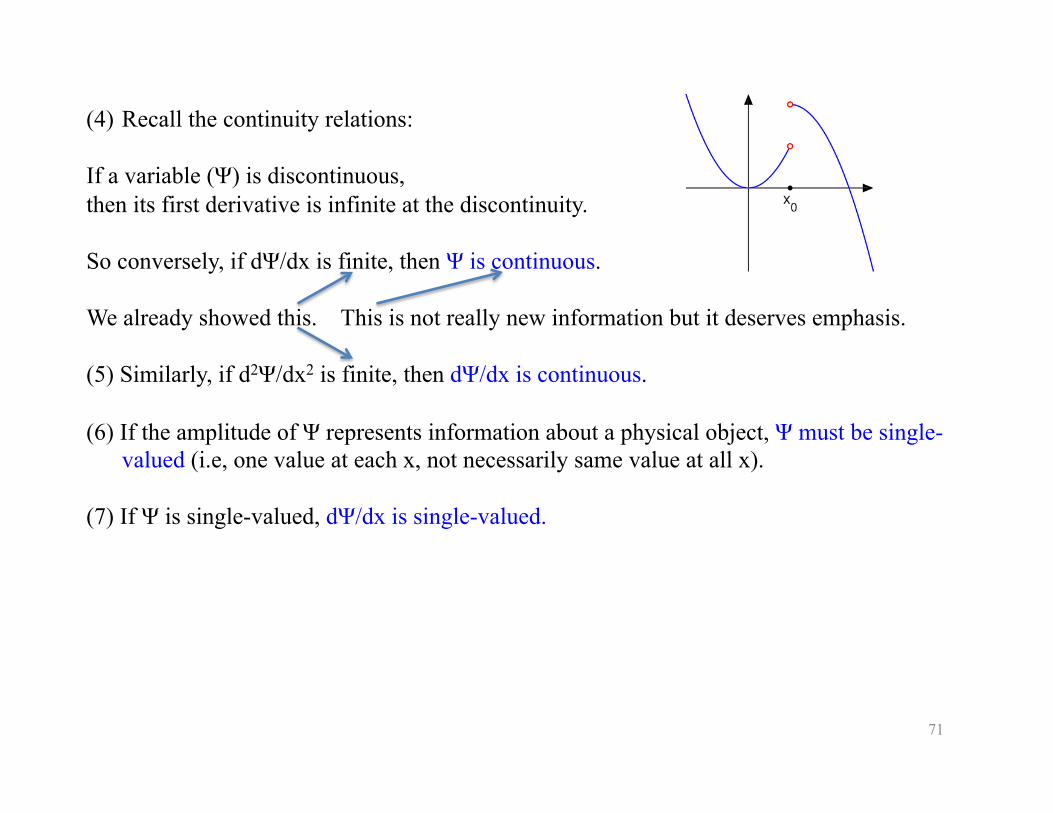
(4) Recall the continuity relations:
If a variable (Ψ) is discontinuous, then its first derivative is infinite at the discontinuity.
So conversely, if dΨ/dx is finite, then Ψ is continuous.
We already showed this. This is not really new information but it deserves emphasis.
(5) Similarly, if d2Ψ/dx2 is finite, then dΨ/dx is continuous.
(6) If the amplitude of Ψ represents information about a physical object, Ψ must be single-valued (i.e, one value at each x, not necessarily same value at all x).
(7) If Ψ is single-valued, dΨ/dx is single-valued.
72
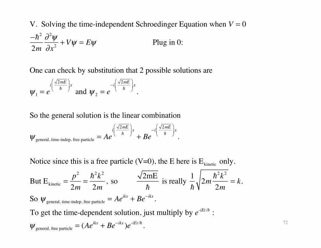
V. Solving the time-independent Schroedinger Equation when V = 0−2
2m∂ 2ψ∂x2 +Vψ = Eψ Plug in 0:
One can check by substitution that 2 possible solutions are
ψ 1 = ei 2mE
⎛
⎝⎜⎞
⎠⎟x
and ψ 2 = e− i 2mE
⎛
⎝⎜⎞
⎠⎟x
.
So the general solution is the linear combination
ψ general, time-indep, free particle = Aei 2mE
⎛
⎝⎜⎞
⎠⎟x
+ Be− i 2mE
⎛
⎝⎜⎞
⎠⎟x
.
Notice since this is a free particle (V=0), the E here is Ekinetic only.
But Ekinetic =p2
2m=
2k2
2m, so 2mE
is really 1
2m
2k2
2m= k.
So ψ general, time-indep, free particle = Aeikx + Be− ikx .
To get the time-dependent solution, just multiply by e-iEt / :ψ general, free particle = (Aeikx + Be− ikx )e-iEt / .
73
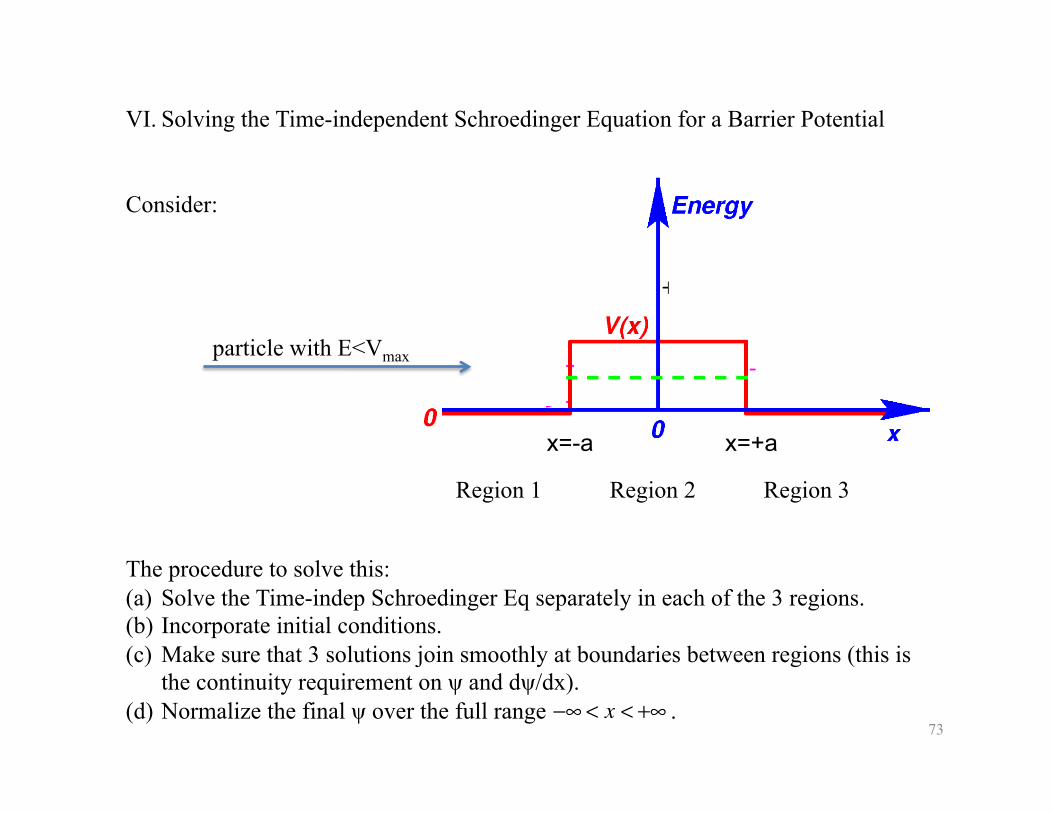
VI. Solving the Time-independent Schroedinger Equation for a Barrier Potential
Consider:
Region 1 Region 2 Region 3
The procedure to solve this: (a) Solve the Time-indep Schroedinger Eq separately in each of the 3 regions. (b) Incorporate initial conditions. (c) Make sure that 3 solutions join smoothly at boundaries between regions (this is
the continuity requirement on ψ and dψ/dx). (d) Normalize the final ψ over the full range .
�
−∞ < x < +∞
particle with E<Vmax
x=-a x=+a
74
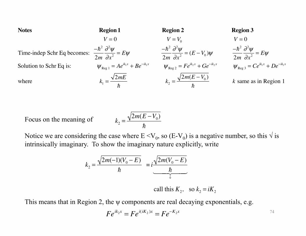
Notes Region 1 Region 2 Region 3 V = 0 V = V0 V = 0
Time-indep Schr Eq becomes: −2
2m∂ 2ψ∂x2 = Eψ −
2
2m∂ 2ψ∂x2 = (E −V0 )ψ −
2
2m∂ 2ψ∂x2 = Eψ
Solution to Schr Eq is: ψ Reg 1 = Aeik1x + Be− ik1x ψ Reg 2 = Fe
ik2 x +Ge− ik2 x ψ Reg 3 = Ceik1x + De− ik1x
where k1 =2mE
k2 =2m(E −V0 )
k same as in Region 1
Focus on the meaning of
Notice we are considering the case where E <V0, so (E-V0) is a negative number, so this √ is intrinsically imaginary. To show the imaginary nature explicitly, write
This means that in Region 2, the ψ components are real decaying exponentials, e.g.
�
k2 =2m(E −V0)
�
k2 =2m(−1)(V0 − E)
= i
2m(V0 − E)↓
call this K2, so k2 = iK2
�
Feik2x = Fei( iK2 )x = Fe−K2x
75
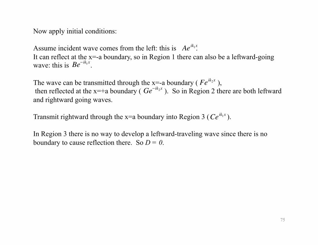
Now apply initial conditions:
Assume incident wave comes from the left: this is . It can reflect at the x=-a boundary, so in Region 1 there can also be a leftward-going wave: this is .
The wave can be transmitted through the x=-a boundary ( ), then reflected at the x=+a boundary ( ). So in Region 2 there are both leftward and rightward going waves.
Transmit rightward through the x=a boundary into Region 3 ( ).
In Region 3 there is no way to develop a leftward-traveling wave since there is no boundary to cause reflection there. So D = 0.
�
Aeik1x
�
Be− ik1x
�
Feik2x
�
Ge−ik2x
�
Ceik1x
76
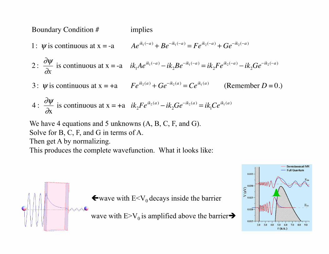
�
Boundary Condition # implies
1: ψ is continuous at x = -a Aeik1 (−a ) + Be−ik1 (−a ) = Feik2 (−a ) + Ge−ik2 (−a )
2 : ∂ψ∂x
is continuous at x = -a ik1Aeik1 (−a ) − ik2Be
−ik1 (−a ) = ik2Feik2 (−a ) − ik2Ge
− ik2 (−a )
3 : ψ is continuous at x = +a Feik2 (a ) + Ge− ik2 (a ) = Ceik1 (a ) (Remember D = 0.)
4 : ∂ψ∂x
is continuous at x = +a ik2Feik2 (a ) − ik2Ge
− ik2 (a ) = ik1Ceik1 (a )
We have 4 equations and 5 unknowns (A, B, C, F, and G). Solve for B, C, F, and G in terms of A. Then get A by normalizing. This produces the complete wavefunction. What it looks like:
wave with E<V0 decays inside the barrier
wave with E>V0 is amplified above the barrier
77
Outline
I. Reflection and Transmission Coefficients II. The response of a particle to being trapped in a square well potential III. Energy of a particle trapped in a square well
78
I. Reflection and transmission coefficients
Consider 2 questions:
1. What is the probability that the original particle is transmitted past any particular boundary?
2. What is the probability that it is reflected at any particular boundary?
Recall probability density ρ(x,t) = ψ*ψ. This is the probability per location x and time t; i.e., the probability that the particle is
located AT point x if one tries to observe it at time t. Now suppose the particle has velocity v, and you want to know its
“probability flux”: probability density PER SECOND that the particle crosses location x, heading in a particular direction.
79
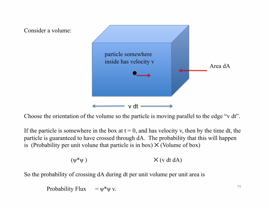
Consider a volume:
Area dA
v dt
particle somewhere inside has velocity v
Choose the orientation of the volume so the particle is moving parallel to the edge “v dt”.
If the particle is somewhere in the box at t = 0, and has velocity v, then by the time dt, the particle is guaranteed to have crossed through dA. The probability that this will happen is (Probability per unit volune that particle is in box) ✕ (Volume of box)
(ψ*ψ ) ✕ (v dt dA)
So the probability of crossing dA during dt per unit volume per unit area is
Probability Flux = ψ*ψ v.
80
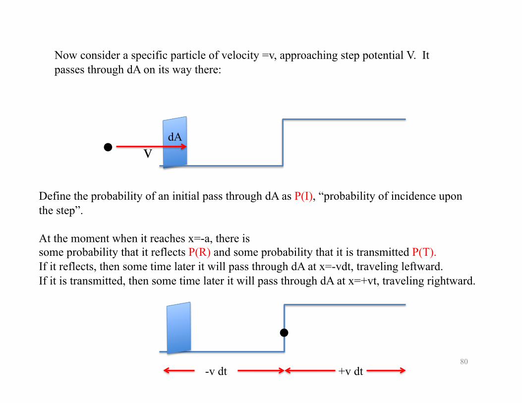
Now consider a specific particle of velocity =v, approaching step potential V. It passes through dA on its way there:
v dA
Define the probability of an initial pass through dA as P(I), “probability of incidence upon the step”.
At the moment when it reaches x=-a, there is some probability that it reflects P(R) and some probability that it is transmitted P(T). If it reflects, then some time later it will pass through dA at x=-vdt, traveling leftward. If it is transmitted, then some time later it will pass through dA at x=+vt, traveling rightward.
-v dt +v dt
81
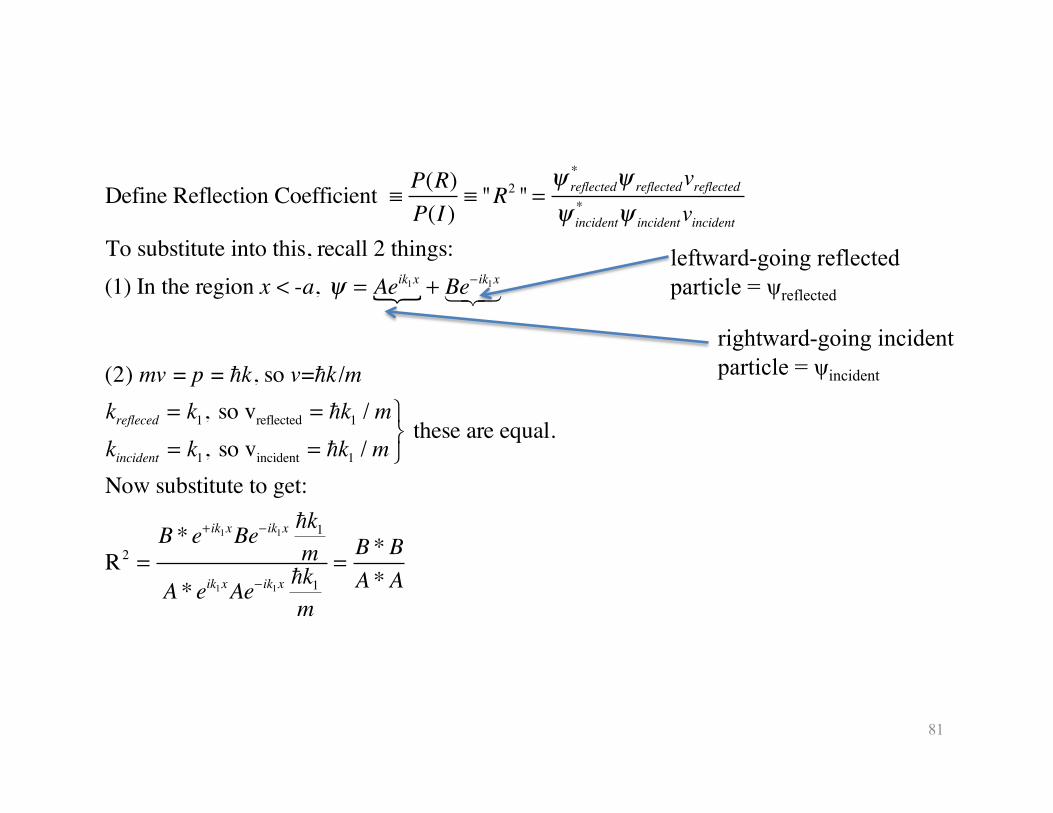
Define Reflection Coefficient ≡ P(R)P(I )
≡ "R2 " =ψ reflected
* ψ reflectedvreflectedψ incident
* ψ incidentvincidentTo substitute into this, recall 2 things:(1) In the region x < -a, ψ = Aeik1x
+ Be− ik1x
(2) mv = p = k, so v=k /mkrefleced = k1, so vreflected = k1 / mkincident = k1, so vincident = k1 / m
⎫⎬⎭
these are equal.
Now substitute to get:
R2 =B * e+ ik1xBe− ik1x k1
mA * eik1xAe− ik1x k1
m
=B * BA * A
leftward-going reflected particle = ψreflected
rightward-going incident particle = ψincident
82
�
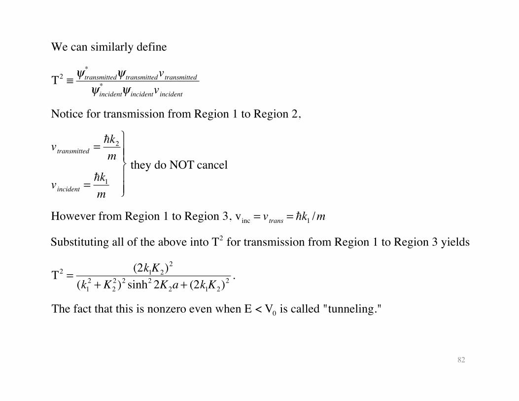
We can similarly define
T2 ≡ ψtransmitted* ψ transmittedvtransmittedψincident
* ψ incidentvincident
Notice for transmission from Region 1 to Region 2,
vtransmitted = k2
m
vincident = k1
m
⎫
⎬ ⎪ ⎪
⎭ ⎪ ⎪
they do NOT cancel
However from Region 1 to Region 3, vinc = vtrans = k1 /m
Substituting all of the above into T2 for transmission from Region 1 to Region 3 yields
T2 = (2k1K2)2
(k12 + K2
2)2 sinh2 2K2a + (2k1K2)2 .
The fact that this is nonzero even when E < V0 is called "tunneling."
83
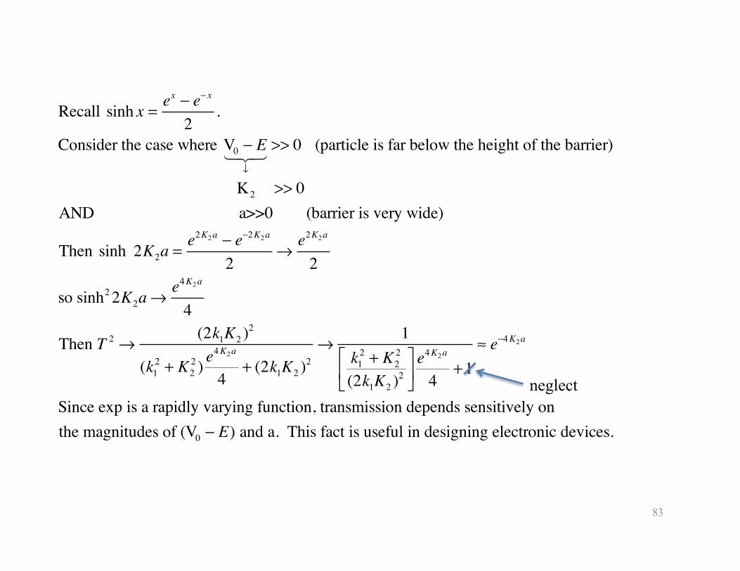
Recall sinh x = ex − e− x
2.
Consider the case where V0 − E↓
>> 0 (particle is far below the height of the barrier)
K2 >> 0AND a>>0 (barrier is very wide)
Then sinh 2K2a =e2K2a − e−2K2a
2→
e2K2a
2
so sinh2 2K2a→e4K2a
4
Then T 2 →(2k1K2 )2
(k12 + K2
2 ) e4K2a
4+ (2k1K2 )2
→1
k12 + K2
2
(2k1K2 )2
⎡
⎣⎢
⎤
⎦⎥e4K2a
4+1
≈ e−4K2a
Since exp is a rapidly varying function, transmission depends sensitively on the magnitudes of (V0 − E) and a. This fact is useful in designing electronic devices.
neglect
84
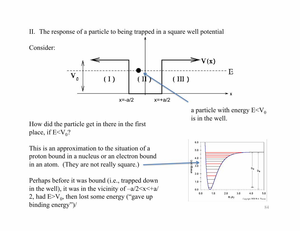
II. The response of a particle to being trapped in a square well potential
Consider:
x=-a/2 x=+a/2
a particle with energy E<V0 is in the well.
How did the particle get in there in the first place, if E<V0?
This is an approximation to the situation of a proton bound in a nucleus or an electron bound in an atom. (They are not really square.)
Perhaps before it was bound (i.e., trapped down in the well), it was in the vicinity of –a/2<x<+a/2, had E>V0, then lost some energy (“gave up binding energy”)/
85
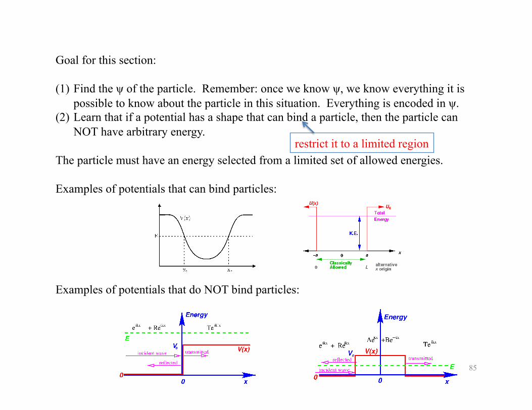
Goal for this section:
(1) Find the ψ of the particle. Remember: once we know ψ, we know everything it is possible to know about the particle in this situation. Everything is encoded in ψ.
(2) Learn that if a potential has a shape that can bind a particle, then the particle can NOT have arbitrary energy.
The particle must have an energy selected from a limited set of allowed energies.
Examples of potentials that can bind particles:
Examples of potentials that do NOT bind particles:
restrict it to a limited region
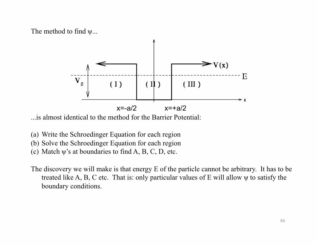
The method to find ψ...
...is almost identical to the method for the Barrier Potential:
(a) Write the Schroedinger Equation for each region (b) Solve the Schroedinger Equation for each region (c) Match ψ’s at boundaries to find A, B, C, D, etc.
The discovery we will make is that energy E of the particle cannot be arbitrary. It has to be treated like A, B, C etc. That is: only particular values of E will allow ψ to satisfy the boundary conditions.
86
x=-a/2 x=+a/2
87
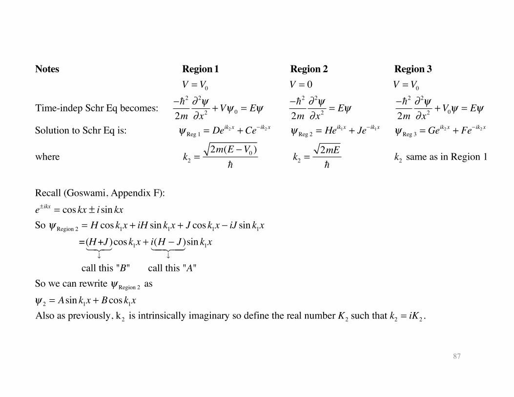
Notes Region 1 Region 2 Region 3 V = V0 V = 0 V = V0
Time-indep Schr Eq becomes: −2
2m∂ 2ψ∂x2 +Vψ 0 = Eψ −
2
2m∂ 2ψ∂x2 = Eψ −
2
2m∂ 2ψ∂x2 +V0ψ = Eψ
Solution to Schr Eq is: ψ Reg 1 = Deik2 x + Ce− ik2 x ψ Reg 2 = He
ik1x + Je− ik1x ψ Reg 3 = Geik2 x + Fe− ik2 x
where k2 =2m(E −V0 )
k2 =2mE
k2 same as in Region 1
Recall (Goswami, Appendix F):e± ikx = coskx ± i sin kxSo ψ Region 2 = H cosk1x + iH sin k1x + J cosk1x − iJ sin k1x =(H+J )
↓
cosk1x + i(H − J )↓
sin k1x
call this "B" call this "A"So we can rewrite ψ Region 2 asψ 2 = Asin k1x + Bcosk1xAlso as previously, k2 is intrinsically imaginary so define the real number K2 such that k2 = iK2 .
88
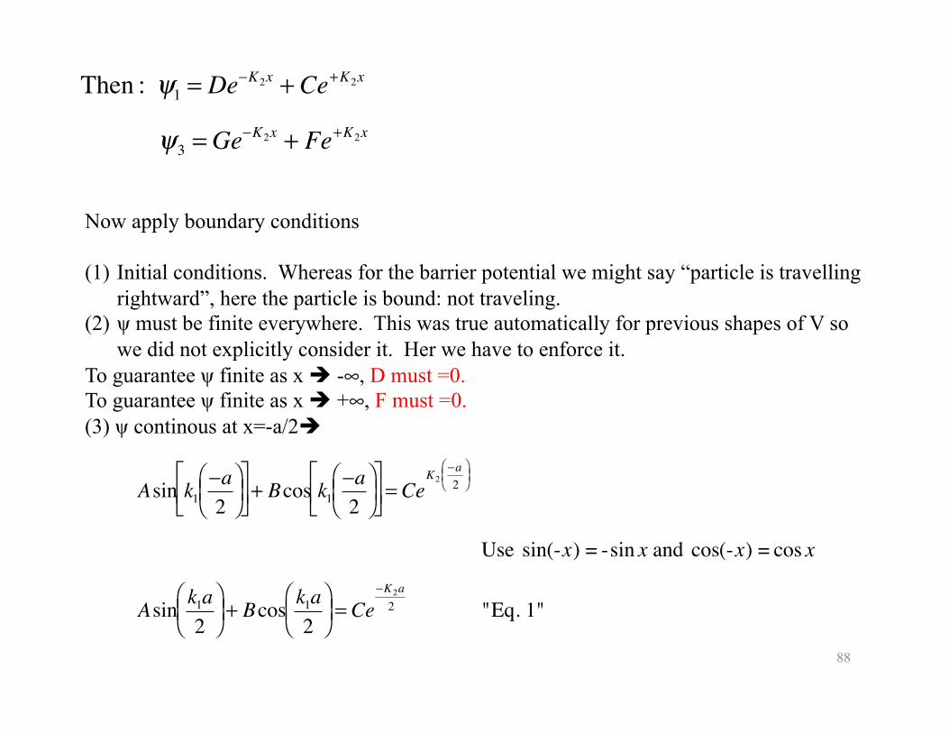
�
Then : ψ1 = De−K2x + Ce+K2x
ψ3 = Ge−K2x + Fe+K2x
Now apply boundary conditions
(1) Initial conditions. Whereas for the barrier potential we might say “particle is travelling rightward”, here the particle is bound: not traveling.
(2) ψ must be finite everywhere. This was true automatically for previous shapes of V so we did not explicitly consider it. Her we have to enforce it.
To guarantee ψ finite as x -∞, D must =0. To guarantee ψ finite as x +∞, F must =0. (3) ψ continous at x=-a/2
�
Asin k1−a2
⎛ ⎝ ⎜
⎞ ⎠ ⎟
⎡ ⎣ ⎢
⎤ ⎦ ⎥ + Bcos k1
−a2
⎛ ⎝ ⎜
⎞ ⎠ ⎟
⎡ ⎣ ⎢
⎤ ⎦ ⎥ = Ce
K2−a2
⎛ ⎝ ⎜
⎞ ⎠ ⎟
Use sin(-x) = -sin x and cos(-x) = cos x
Asin k1a2
⎛ ⎝ ⎜
⎞ ⎠ ⎟ + Bcos k1a
2⎛ ⎝ ⎜
⎞ ⎠ ⎟ = Ce
−K2a2 "Eq. 1"
89
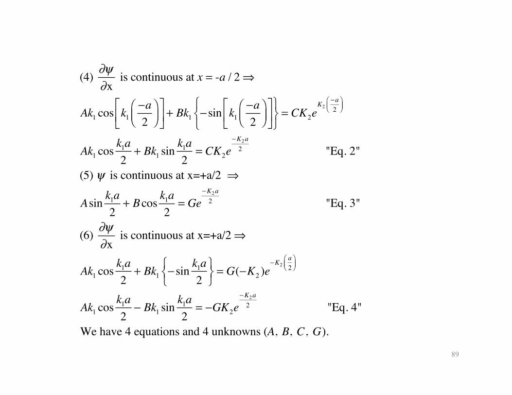
(4) ∂ψ∂x
is continuous at x = -a / 2 ⇒
Ak1 cos k1−a2
⎛⎝⎜
⎞⎠⎟
⎡⎣⎢
⎤⎦⎥+ Bk1 − sin k1
−a2
⎛⎝⎜
⎞⎠⎟
⎡⎣⎢
⎤⎦⎥
⎧⎨⎩
⎫⎬⎭= CK2e
K2−a2
⎛⎝⎜
⎞⎠⎟
Ak1 cos k1a2
+ Bk1 sin k1a2
= CK2e−K2a
2 "Eq. 2"
(5) ψ is continuous at x=+a/2 ⇒
Asin k1a2
+ Bcos k1a2
= Ge−K2a
2 "Eq. 3"
(6) ∂ψ∂x
is continuous at x=+a/2 ⇒
Ak1 cos k1a2
+ Bk1 − sin k1a2
⎧⎨⎩
⎫⎬⎭= G(−K2 )e
−K2a2
⎛⎝⎜
⎞⎠⎟
Ak1 cos k1a2
− Bk1 sin k1a2
= −GK2e−K2a
2 "Eq. 4"
We have 4 equations and 4 unknowns (A, B, C, G).
90
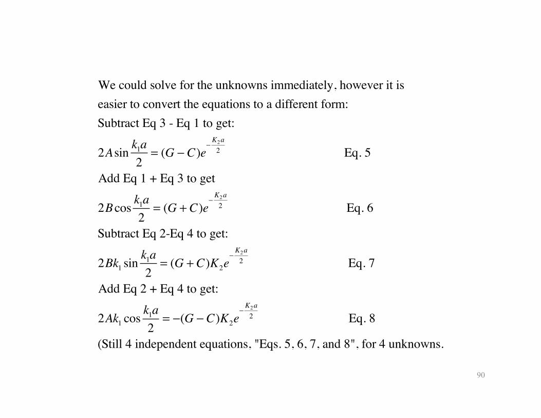
We could solve for the unknowns immediately, however it iseasier to convert the equations to a different form:Subtract Eq 3 - Eq 1 to get:
2Asin k1a2
= (G − C)e−K2a
2 Eq. 5
Add Eq 1 + Eq 3 to get
2Bcos k1a2
= (G + C)e−K2a
2 Eq. 6
Subtract Eq 2-Eq 4 to get:
2Bk1 sin k1a2
= (G + C)K2e−K2a
2 Eq. 7
Add Eq 2 + Eq 4 to get:
2Ak1 cos k1a2
= −(G − C)K2e−K2a
2 Eq. 8
(Still 4 independent equations, "Eqs. 5, 6, 7, and 8", for 4 unknowns.
91
�
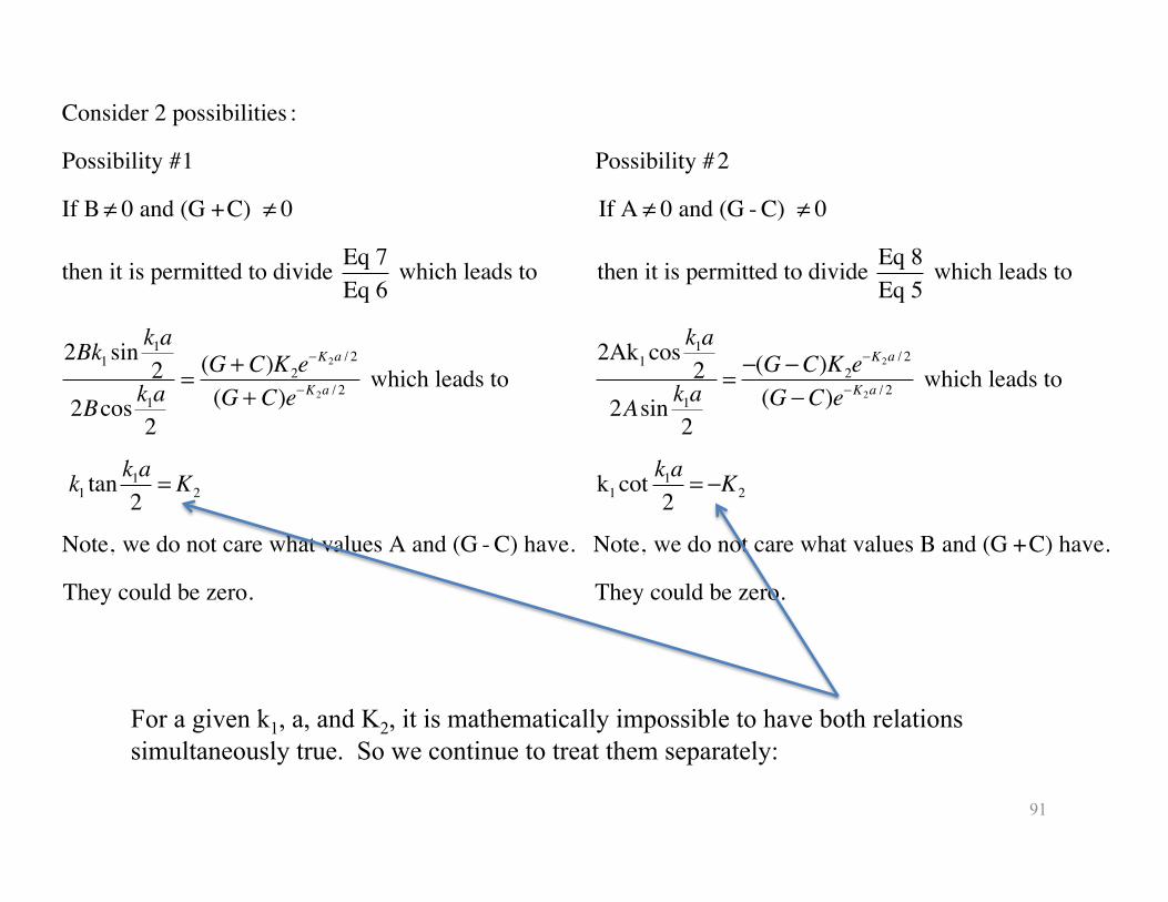
Consider 2 possibilities :
Possibility #1 Possibility #2
If B≠ 0 and (G +C) ≠ 0 If A ≠ 0 and (G - C) ≠ 0
then it is permitted to divide Eq 7Eq 6
which leads to then it is permitted to divide Eq 8Eq 5
which leads to
2Bk1 sin k1a2
2Bcos k1a2
= (G + C)K2e−K2a / 2
(G + C)e−K2a / 2 which leads to 2Ak1 cos k1a
22Asin k1a
2
= −(G −C)K2e−K2a / 2
(G −C)e−K2a / 2 which leads to
k1 tan k1a2
= K2 k1 cot k1a2
= −K2
Note, we do not care what values A and (G - C) have. Note, we do not care what values B and (G +C) have.
They could be zero. They could be zero.
For a given k1, a, and K2, it is mathematically impossible to have both relations simultaneously true. So we continue to treat them separately:
92
�
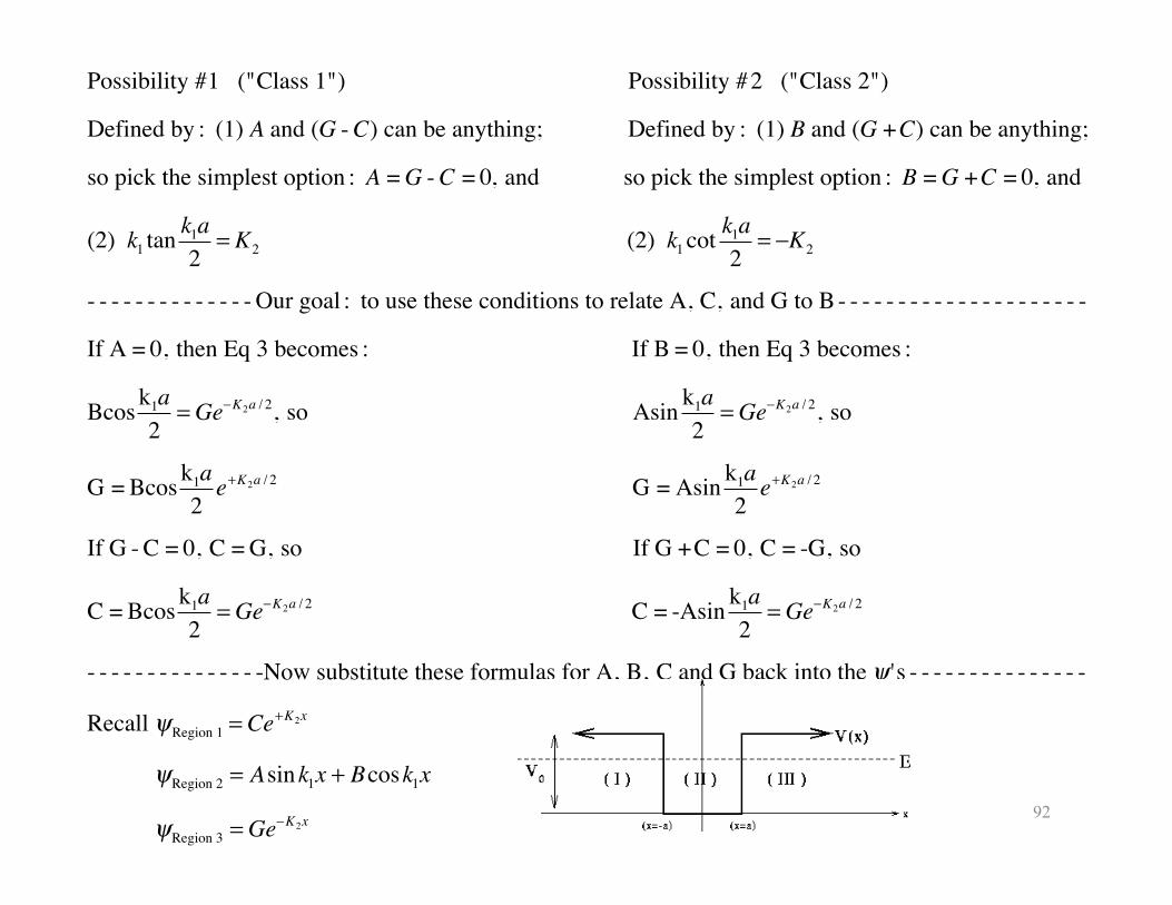
Possibility #1 ("Class 1") Possibility #2 ("Class 2")
Defined by : (1) A and (G -C) can be anything; Defined by : (1) B and (G +C) can be anything;
so pick the simplest option : A =G -C = 0, and so pick the simplest option : B =G +C = 0, and
(2) k1 tan k1a2
= K2 (2) k1 cot k1a2
= −K2
- - - - - - - - - - - - - - Our goal : to use these conditions to relate A, C, and G to B - - - - - - - - - - - - - - - - - - - - -
If A = 0, then Eq 3 becomes : If B = 0, then Eq 3 becomes :
Bcos k1a2
= Ge−K2a / 2, so Asin k1a2
= Ge−K2a / 2, so
G = Bcos k1a2e+K2a / 2 G = Asin k1a
2e+K2a / 2
If G - C = 0, C = G, so If G +C = 0, C = -G, so
C = Bcos k1a2
= Ge−K2a / 2 C = -Asin k1a2
= Ge−K2a / 2
- - - - - - - - - - - - - - -Now substitute these formulas for A, B, C and G back into the ψ 's - - - - - - - - - - - - - - -
Recall ψRegion 1 = Ce+K2x
ψRegion 2 = Asink1x + Bcosk1x
ψRegion 3 = Ge−K2x
93
�
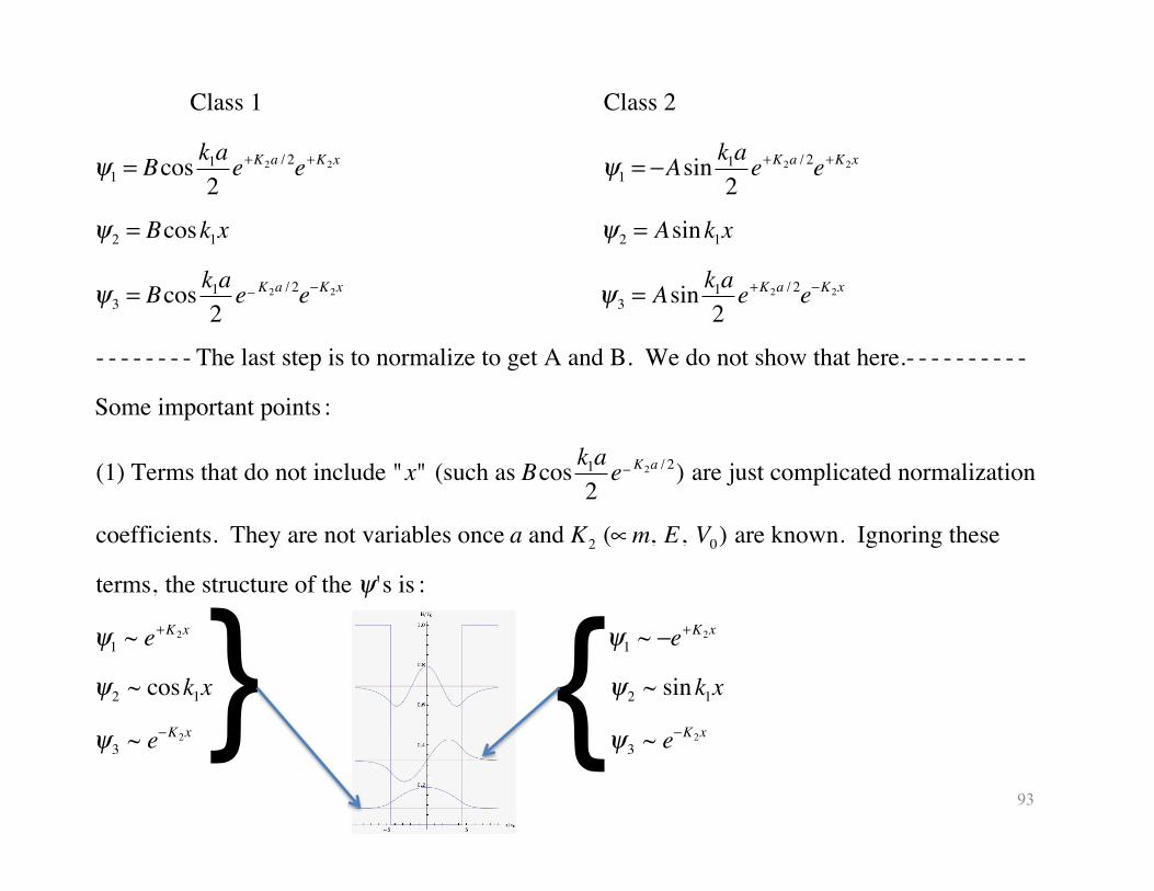
Class 1 Class 2
ψ1 = Bcos k1a2e+K2a / 2e+K2x ψ1 = −Asin k1a
2e+K2a / 2e+K2x
ψ2 = Bcosk1x ψ2 = Asink1x
ψ3 = Bcos k1a2e_ K2a / 2e−K2x ψ3 = Asin k1a
2e+K2a / 2e−K2x
- - - - - - - - The last step is to normalize to get A and B. We do not show that here.- - - - - - - - - -
Some important points :
(1) Terms that do not include "x" (such as Bcos k1a2e_ K2a / 2) are just complicated normalization
coefficients. They are not variables once a and K2 (∝m, E, V0) are known. Ignoring these
terms, the structure of the ψ's is :
ψ1 ~ e+K2x ψ1 ~ −e+K2x
ψ2 ~ cosk1x ψ2 ~ sink1x
ψ3 ~ e−K2x ψ3 ~ e−K2x} {
94
�
(2) The exponentials in Regions 1 and 3 are like those in the barrier potential.
(3) In Region 2, the ψ can be either cos or sine. So the full time - dependent wave functions are
Class 1 Class 2
Ψ2 ~ cos(k1x)e−iEt / Ψ2 ~ sin(k1x)e−iEt /
Notice : as t changes, x does not need to change to preserve the cosine or sine waveform- - -
so both cases are standing waves : the particle is trapped in the well, not traveling.
95
III. Energy of a particle trapped in a square well
The message of this section is:
A particle in a well cannot have any arbitrary energy. To satisfy all the boundary conditions, only certain energies are allowed.
How to find the allowed energies:
Recall that there are 2 classes of wavefunctions ψ supported by the square well. Each has its own relationship between k1 and K2:
�
Class 1 Class 2
k1 tan k1a2
= K2 k1 cot k1a2
= −K2
where :
k1 ≡2mE
and K2 ≡2m(V0 − E)
.
Substitute for k1 and K2 and solve for E :
96
�
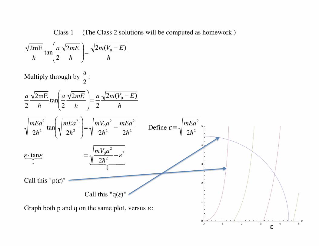
Class 1 (The Class 2 solutions will be computed as homework.)
2mE
tan a2
2mE
⎛
⎝ ⎜
⎞
⎠ ⎟ =
2m(V0 − E)
Multiply through by a2
:
a2
2mE
tan a2
2mE
⎛
⎝ ⎜
⎞
⎠ ⎟ = a
22m(V0 − E)
mEa2
22 tan mEa2
22
⎛
⎝ ⎜ ⎜
⎞
⎠ ⎟ ⎟ = mV0a
2
22 − mEa2
22 Define ε ≡ mEa2
22 . Then,
ε ⋅ tanε↓
= mV0a2
22 −ε2
↓
Call this "p(ε)"
Call this "q(ε)"
Graph both p and q on the same plot, versus ε :
ε
97
�
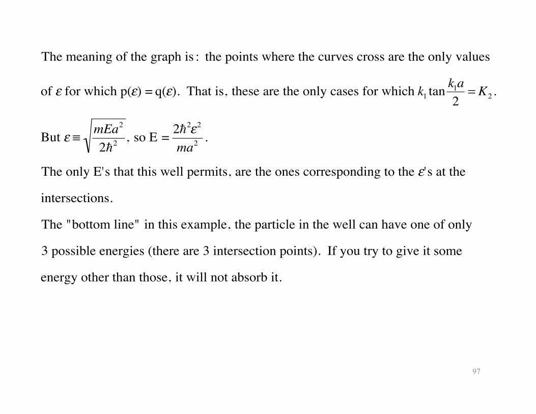
The meaning of the graph is : the points where the curves cross are the only values
of ε for which p(ε) = q(ε). That is, these are the only cases for which k1 tan k1a2
= K2 .
But ε ≡ mEa2
22 , so E = 22ε2
ma2 .
The only E's that this well permits, are the ones corresponding to the ε's at the
intersections.
The "bottom line" in this example, the particle in the well can have one of only
3 possible energies (there are 3 intersection points). If you try to give it some
energy other than those, it will not absorb it.
98
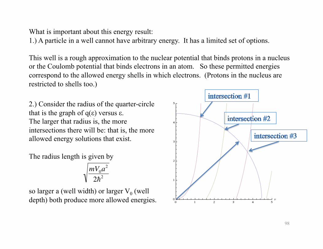
What is important about this energy result: 1.) A particle in a well cannot have arbitrary energy. It has a limited set of options.
This well is a rough approximation to the nuclear potential that binds protons in a nucleus or the Coulomb potential that binds electrons in an atom. So these permitted energies correspond to the allowed energy shells in which electrons. (Protons in the nucleus are restricted to shells too.)
2.) Consider the radius of the quarter-circle that is the graph of q(ε) versus ε. The larger that radius is, the more intersections there will be: that is, the more allowed energy solutions that exist.
The radius length is given by
so larger a (well width) or larger V0 (well depth) both produce more allowed energies.
�
mV0a2
22
99
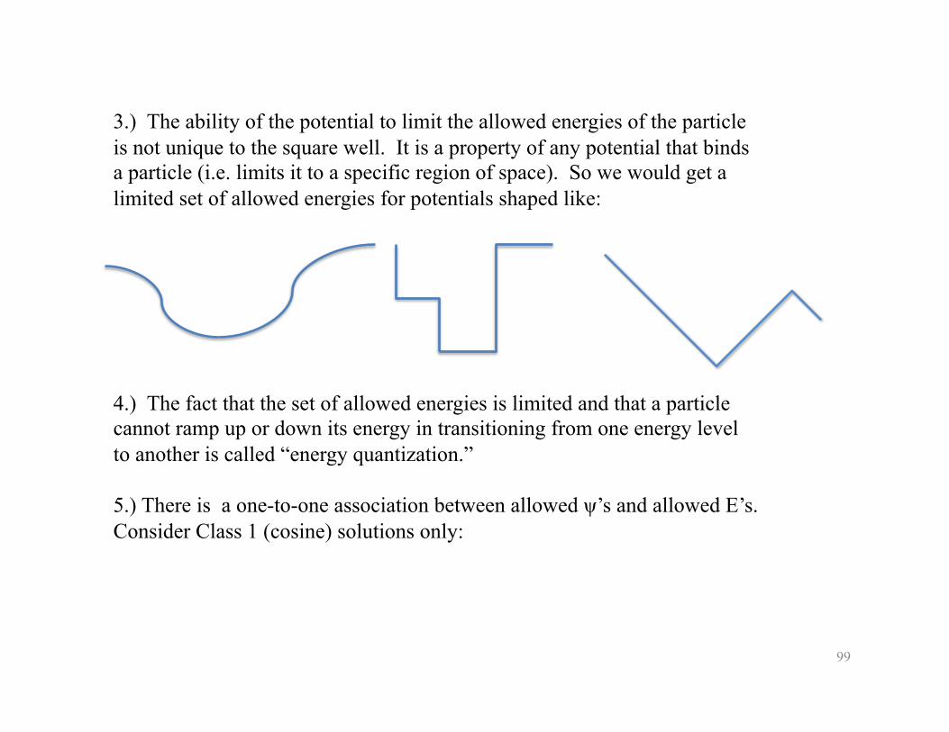
3.) The ability of the potential to limit the allowed energies of the particle is not unique to the square well. It is a property of any potential that binds a particle (i.e. limits it to a specific region of space). So we would get a limited set of allowed energies for potentials shaped like:
4.) The fact that the set of allowed energies is limited and that a particle cannot ramp up or down its energy in transitioning from one energy level to another is called “energy quantization.”
5.) There is a one-to-one association between allowed ψ’s and allowed E’s. Consider Class 1 (cosine) solutions only:
100
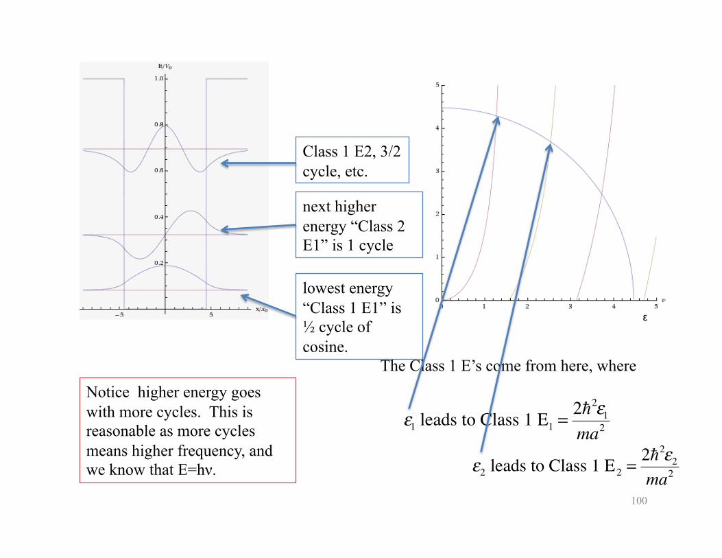
lowest energy “Class 1 E1” is ½ cycle of cosine.
next higher energy “Class 2 E1” is 1 cycle
Class 1 E2, 3/2 cycle, etc.
The Class 1 E’s come from here, where
�
ε1 leads to Class 1 E1 = 22ε1
ma2
�
ε2 leads to Class 1 E2 = 22ε2
ma2
ε
Notice higher energy goes with more cycles. This is reasonable as more cycles means higher frequency, and we know that E=hν.
101
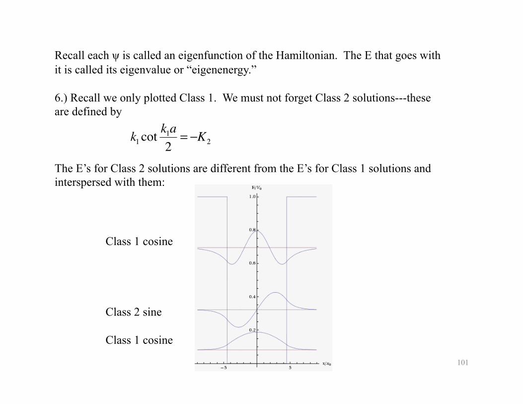
Recall each ψ is called an eigenfunction of the Hamiltonian. The E that goes with it is called its eigenvalue or “eigenenergy.”
6.) Recall we only plotted Class 1. We must not forget Class 2 solutions---these are defined by
The E’s for Class 2 solutions are different from the E’s for Class 1 solutions and interspersed with them:
�
k1 cotk1a2
= −K2
Class 1 cosine
Class 2 sine
Class 1 cosine