Hypothesis
77
Tests of Hypothesis Hypothesis
-
Upload
nilanjan-bhaumik -
Category
Data & Analytics
-
view
110 -
download
1
Transcript of Hypothesis
Tests of HypothesisHypothesis
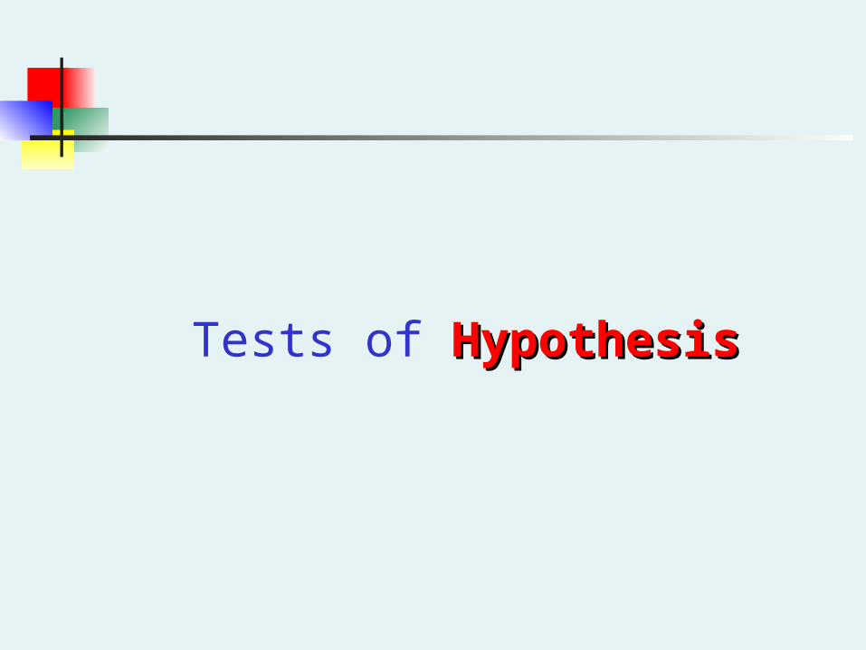
What is a Hypothesis?
A hypothesis is a claim (assumption) about a population parameter:
population mean
population proportion
Example: The mean monthly cell phone bill in this city is μ = $42
Example: The proportion of adults in this city with cell phones is π = 0.68
The Null Hypothesis, H0
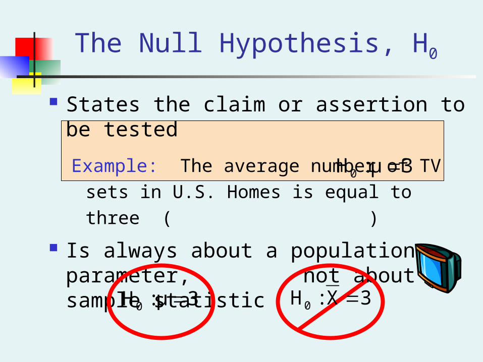
States the claim or assertion to be tested
Example: The average number of TV sets in
U.S. Homes is equal to three ( )
Is always about a population parameter, not about a sample statistic
3μ:H0
3μ:H0 3X:H0
The Null Hypothesis, H0
Begin with the assumption that the null hypothesis is true Similar to the notion of innocent until
proven guilty
Refers to the status quo or historical value Always contains “=” , “≤” or “” sign May or may not be rejected
(continued)
The Alternative Hypothesis, H1
Is the opposite of the null hypothesis e.g., The average number of TV sets in U.S.
homes is not equal to 3 ( H1: μ ≠ 3 )
Challenges the status quo May or may not be proven Is generally the hypothesis that the
researcher is trying to prove
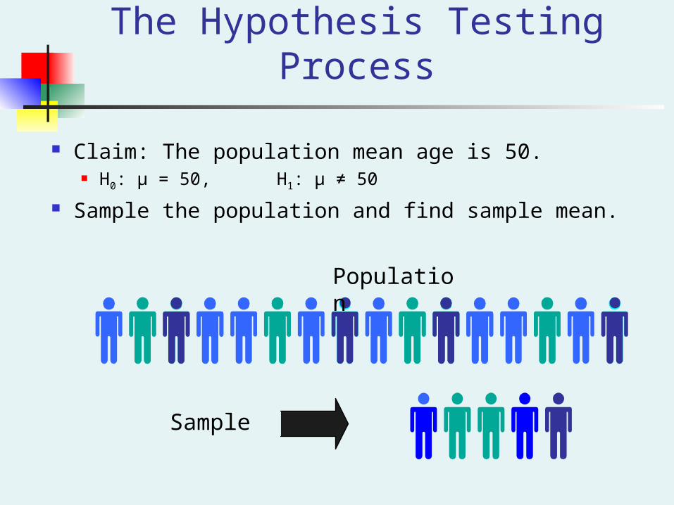
The Hypothesis Testing Process
Claim: The population mean age is 50. H0: μ = 50, H1: μ ≠ 50
Sample the population and find sample mean.
Population
Sample
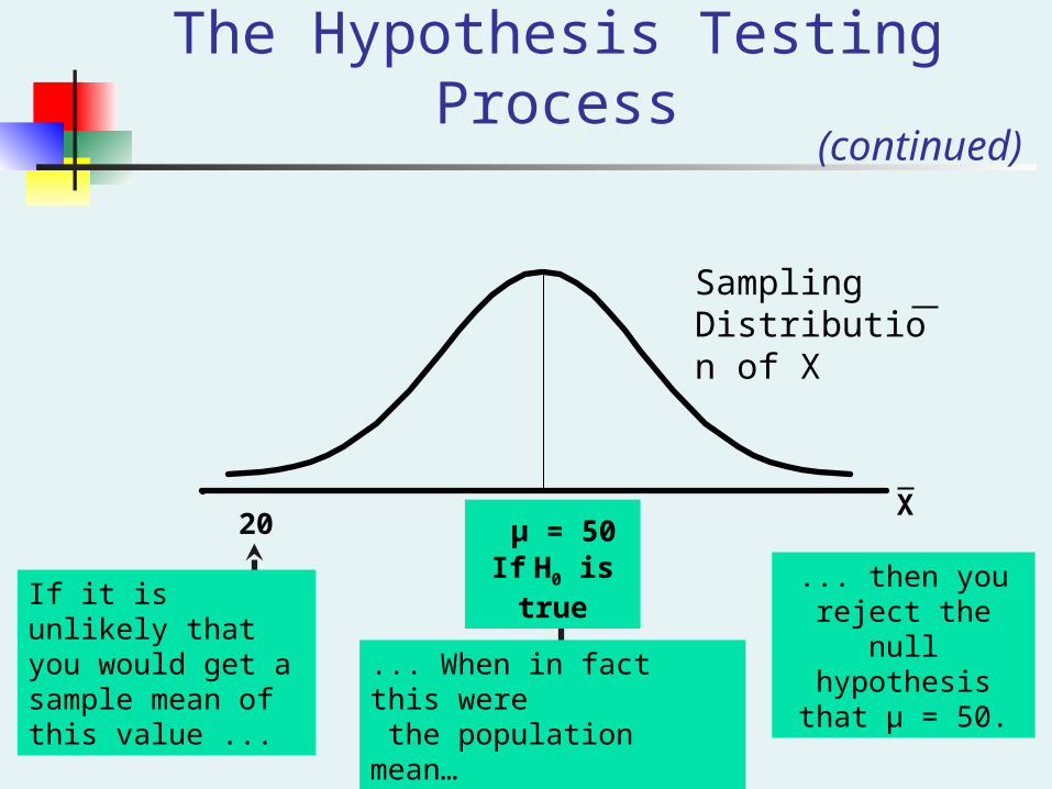
The Hypothesis Testing Process
Sampling Distribution of X
μ = 50If H0 is true
If it is unlikely that you would get a sample mean of this value ...
... then you reject the null hypothesis
that μ = 50.
20
... When in fact this were the population mean…
X
(continued)
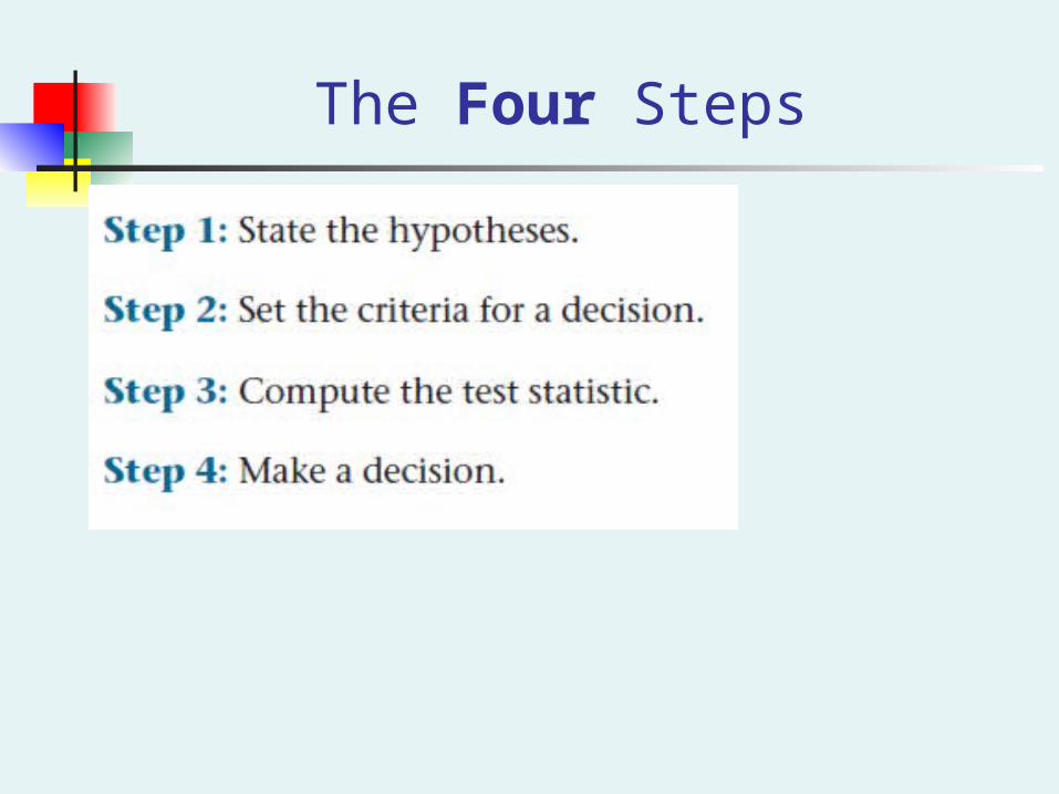
The Four Steps
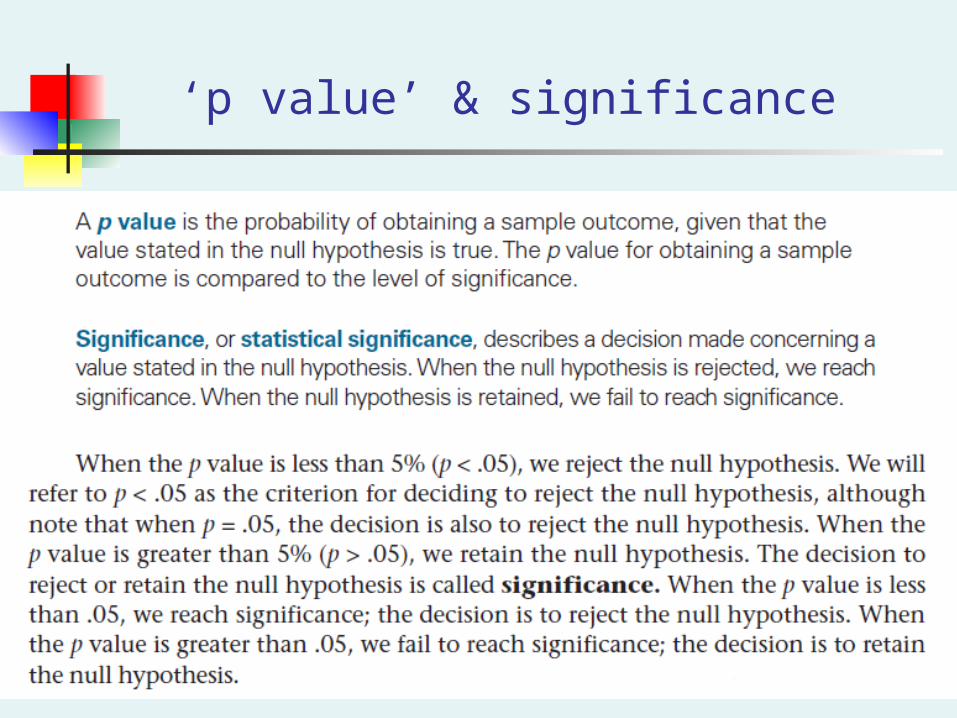
‘p value’ & significance
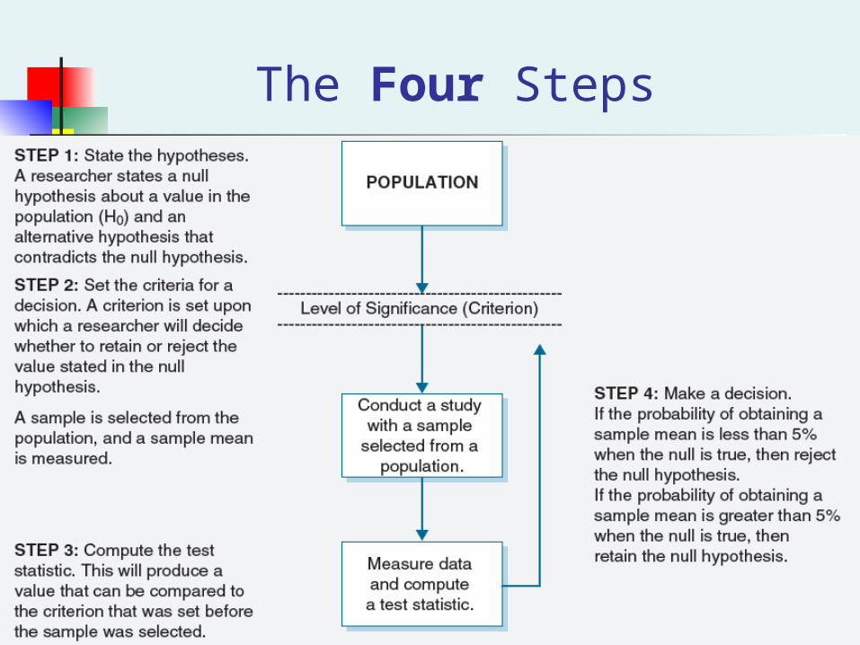
The Four Steps
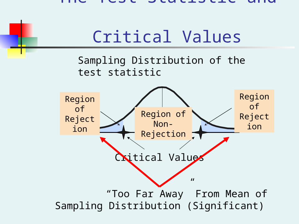
The Test Statistic and Critical Values
Critical Values
“Too Far Away” From Mean of Sampling Distribution (Significant)
Sampling Distribution of the test statistic
Region of Rejection
Region of Rejection
Region ofNon-Rejection
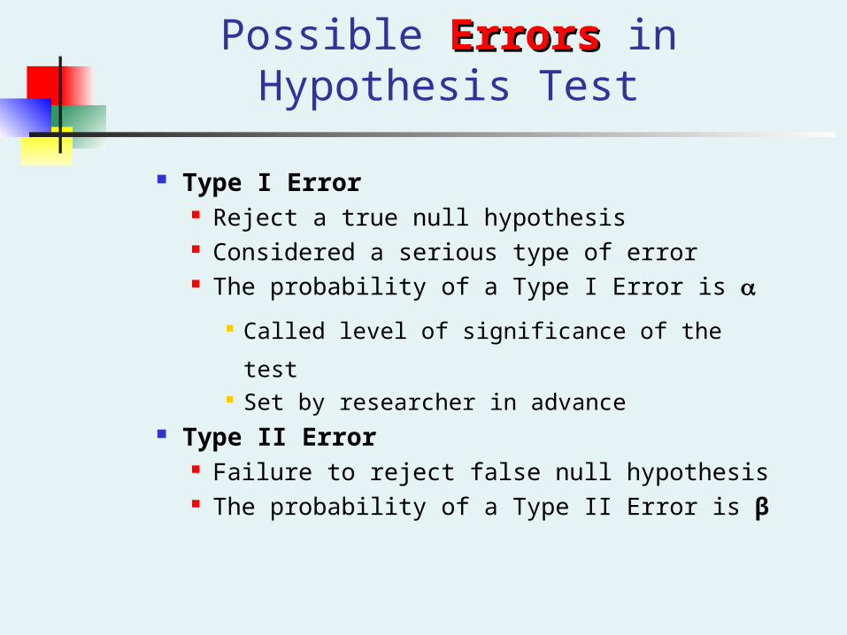
Possible ErrorsErrors in Hypothesis Test
Type I Error Reject a true null hypothesis Considered a serious type of error The probability of a Type I Error is
Called level of significance of the test Set by researcher in advance
Type II Error Failure to reject false null hypothesis The probability of a Type II Error is β
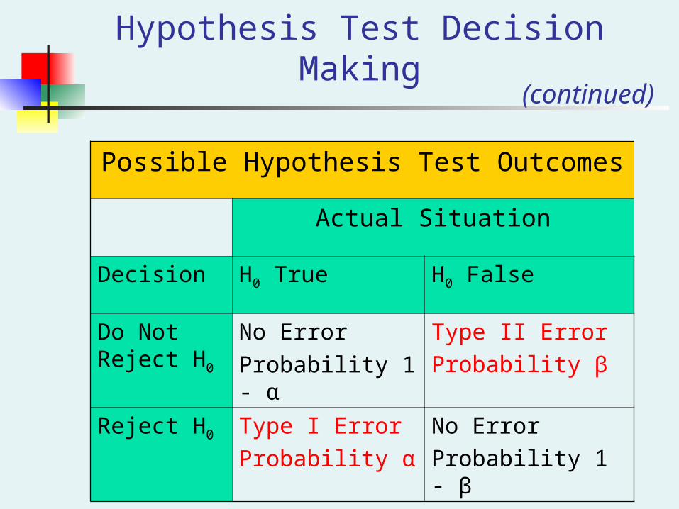
Possible Errors in Hypothesis Test Decision Making
Possible Hypothesis Test Outcomes
Actual Situation
Decision H0 True H0 False
Do Not Reject H0
No Error
Probability 1 - α
Type II Error
Probability β
Reject H0 Type I Error
Probability α
No Error
Probability 1 - β
(continued)
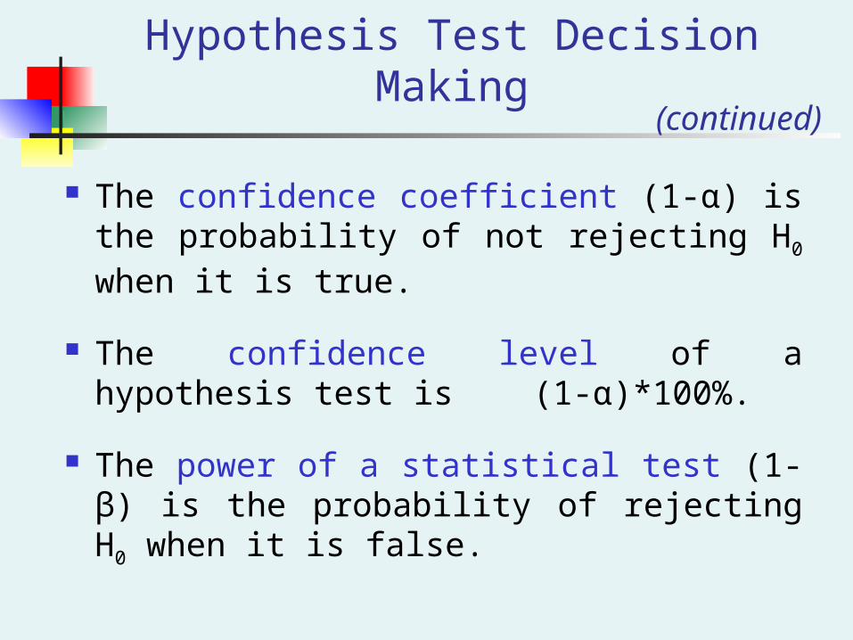
Possible Errors in Hypothesis Test Decision Making
The confidence coefficient (1-α) is the probability of not rejecting H0 when it is true.
The confidence level of a hypothesis test is (1-α)*100%.
The power of a statistical test (1-β) is the probability of rejecting H0 when it is false.
(continued)
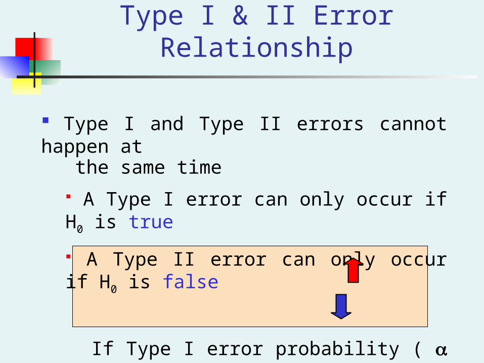
Type I & II Error Relationship
Type I and Type II errors cannot happen at the same time
A Type I error can only occur if H0 is true
A Type II error can only occur if H0 is false
If Type I error probability ( ) , then
Type II error probability ( β )
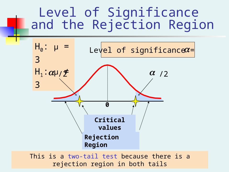
Level of Significance and the Rejection Region
Level of significance =
This is a two-tail test because there is a rejection region in both tails
H0: μ = 3
H1: μ ≠
3
Critical values
Rejection Region
/2
0
/2
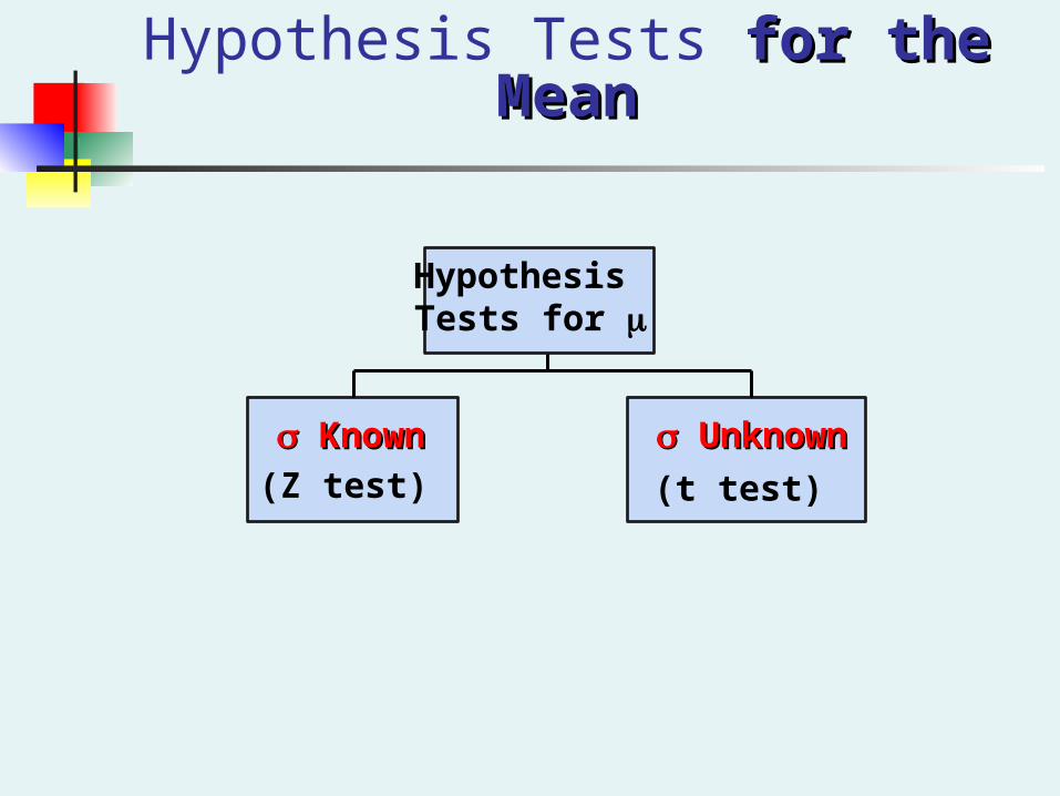
Hypothesis Tests for the Meanfor the Mean
KnownKnown UnknownUnknown
Hypothesis Tests for
(Z test) (t test)
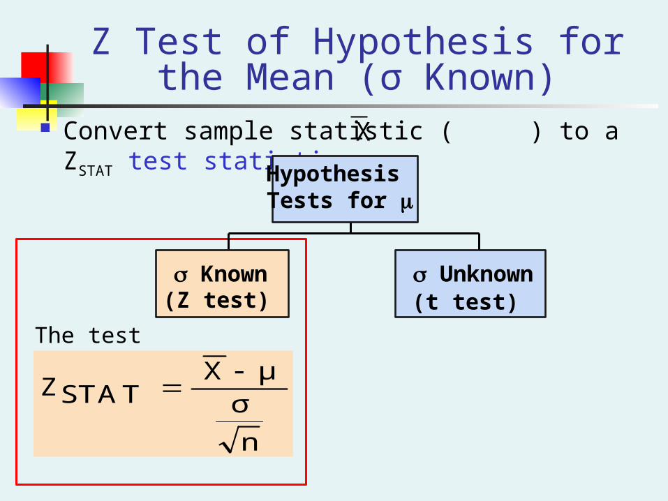
Z Test of Hypothesis for the Mean (σ Known)
Convert sample statistic ( ) to a ZSTAT test statistic X
The test statistic is:
n
σμX
STATZ
σ Known σ Unknown
Hypothesis Tests for
Known Unknown(Z test) (t test)
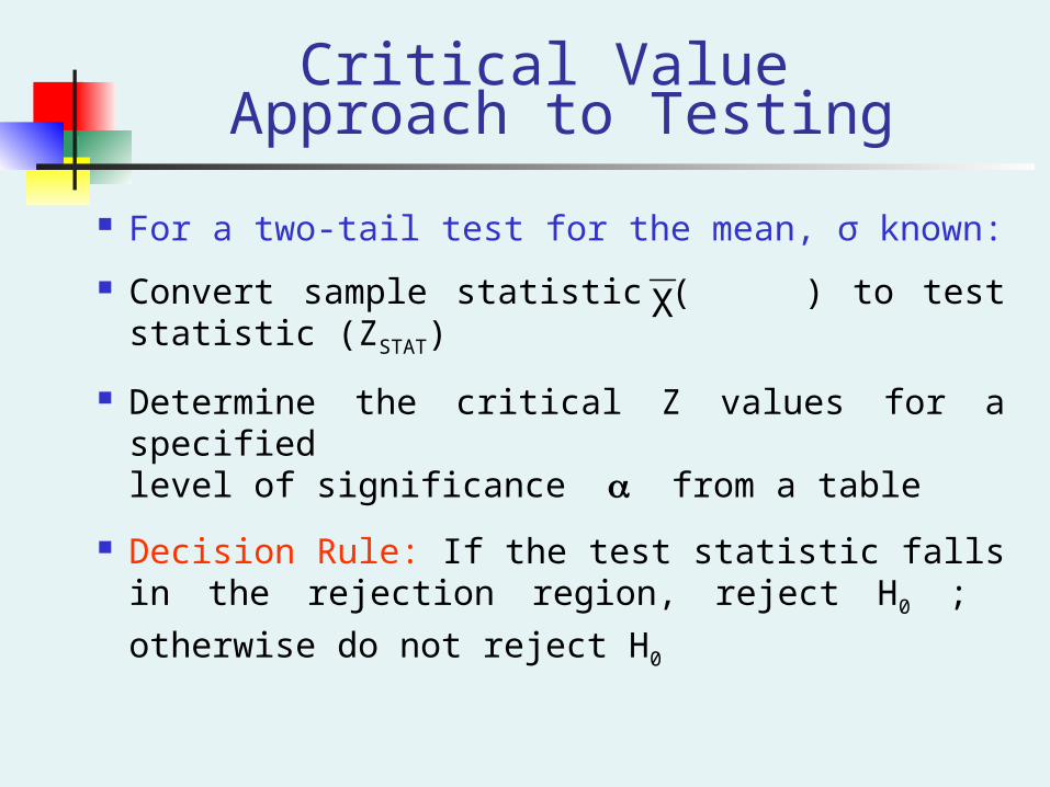
Critical Value Approach to Testing
For a two-tail test for the mean, σ known:
Convert sample statistic ( ) to test statistic (ZSTAT)
Determine the critical Z values for a specifiedlevel of significance from a table
Decision Rule: If the test statistic falls in the rejection region, reject H0 ; otherwise do not
reject H0
X
Do not reject H0 Reject H0Reject H0
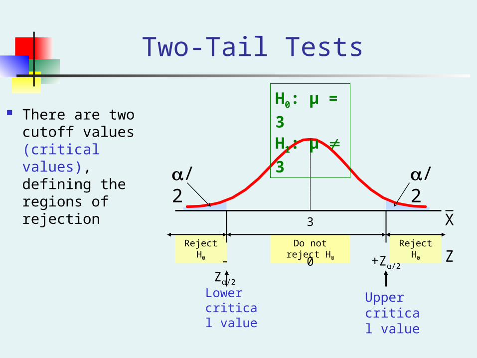
There are two cutoff values (critical values), defining the regions of rejection
Two-Tail Tests
/2
-Zα/2 0
H0: μ = 3
H1: μ
3
+Zα/2
/2
Lower critical value
Upper critical value
3
Z
X
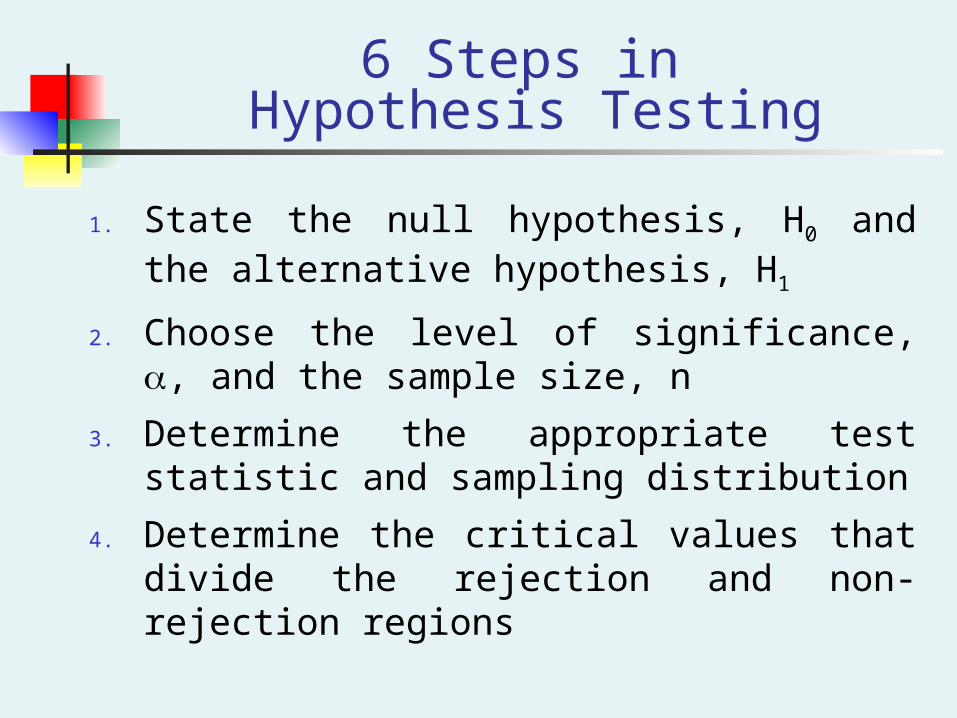
6 Steps in Hypothesis Testing
1. State the null hypothesis, H0 and the alternative hypothesis, H1
2. Choose the level of significance, , and the sample size, n
3. Determine the appropriate test statistic and sampling distribution
4. Determine the critical values that divide the rejection and non-rejection regions
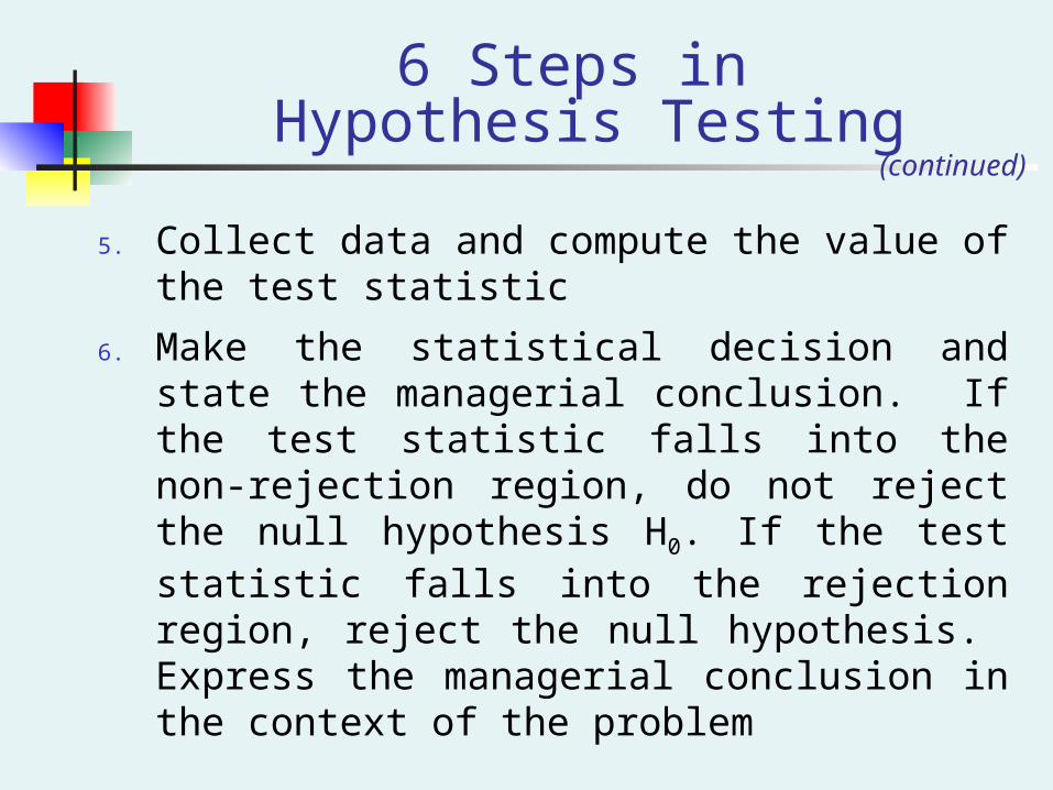
6 Steps in Hypothesis Testing
5. Collect data and compute the value of the test statistic
6. Make the statistical decision and state the managerial conclusion. If the test statistic falls into the non-rejection region, do not reject the null hypothesis H0. If the test statistic falls into the rejection region, reject the null hypothesis. Express the managerial conclusion in the context of the problem
(continued)
Hypothesis Testing Example
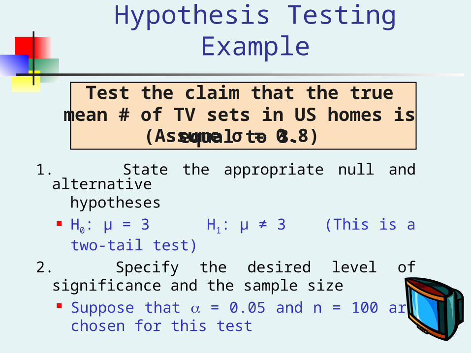
Test the claim that the true mean # of TV sets in US homes is equal to 3.
(Assume σ = 0.8)
1. State the appropriate null and alternative hypotheses
H0: μ = 3 H1: μ ≠ 3 (This is a two-tail test)
2. Specify the desired level of significance and the sample size Suppose that = 0.05 and n = 100 are chosen
for this test
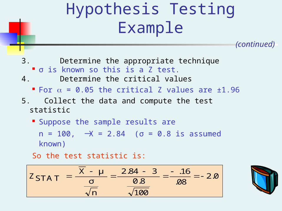
2.0.08
.16
100
0.832.84
n
σμX
STATZ
Hypothesis Testing Example
3. Determine the appropriate technique σ is known so this is a Z test.
4. Determine the critical values For = 0.05 the critical Z values are ±1.96
5. Collect the data and compute the test statistic Suppose the sample results are
n = 100, X = 2.84 (σ = 0.8 is assumed known)
So the test statistic is:
(continued)
Reject H0 Do not reject H0
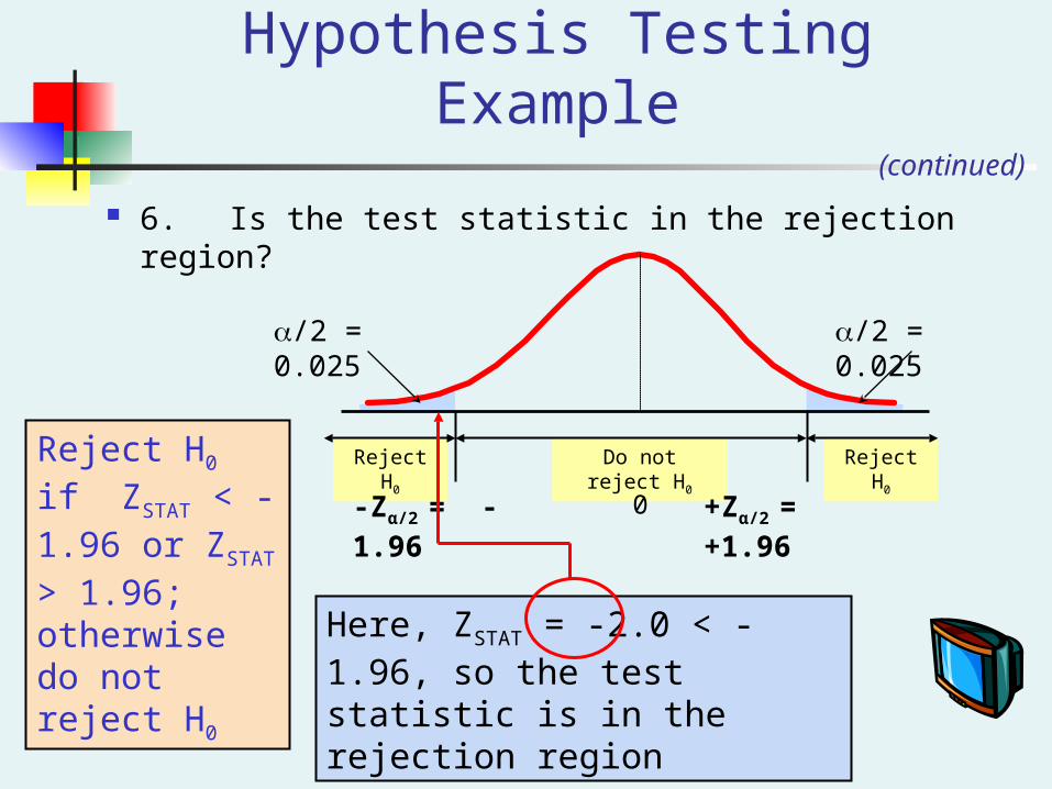
6. Is the test statistic in the rejection region?
/2 = 0.025
-Zα/2 = -1.96 0
Reject H0 if ZSTAT < -1.96 or ZSTAT > 1.96; otherwise do not reject H0
Hypothesis Testing Example(continued)
/2 = 0.025
Reject H0
+Zα/2 = +1.96
Here, ZSTAT = -2.0 < -1.96, so the test statistic is in the rejection region
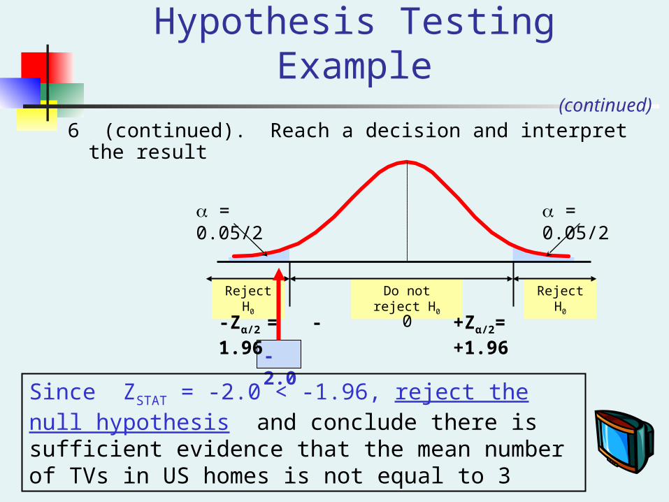
6 (continued). Reach a decision and interpret the result
-2.0
Since ZSTAT = -2.0 < -1.96, reject the null hypothesis and conclude there is sufficient evidence that the mean number of TVs in US homes is not equal to 3
Hypothesis Testing Example(continued)
Reject H0 Do not reject H0
= 0.05/2
-Zα/2 = -1.96 0
= 0.05/2
Reject H0
+Zα/2= +1.96
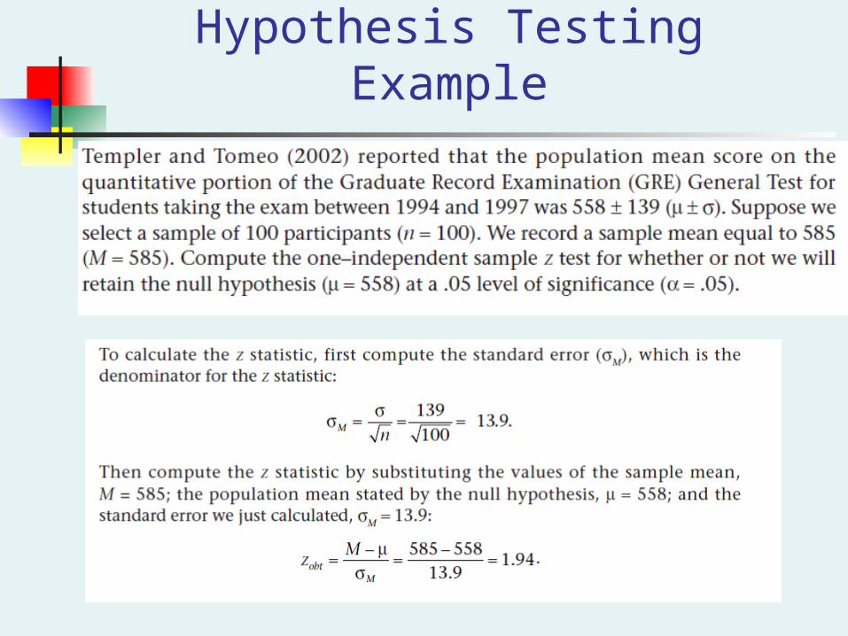
Hypothesis Testing Example
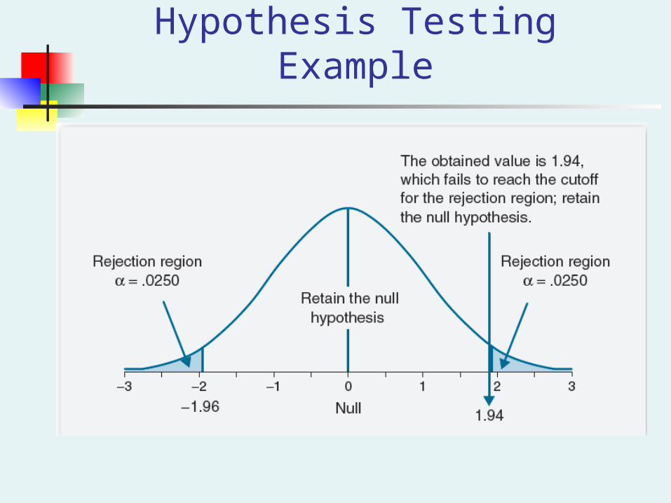
Hypothesis Testing Example
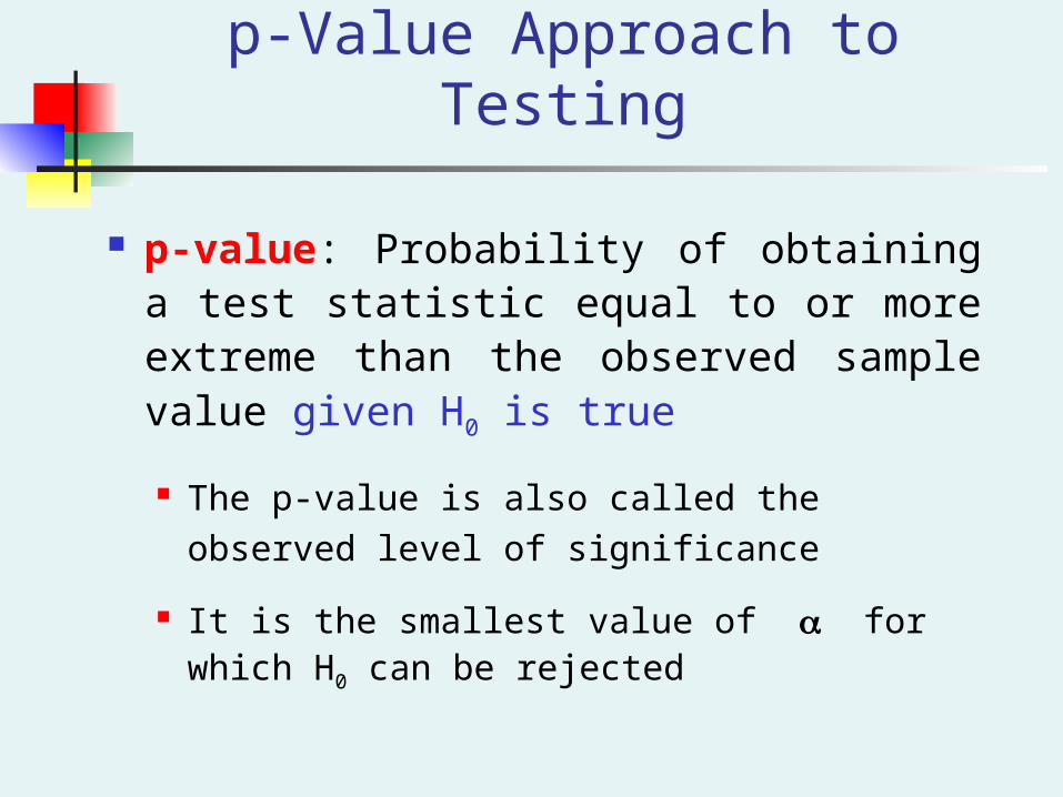
p-Value Approach to Testing
p-value: Probability of obtaining a test statistic equal to or more extreme than the observed sample value given H0 is true
The p-value is also called the observed level of
significance
It is the smallest value of for which H0 can be
rejected
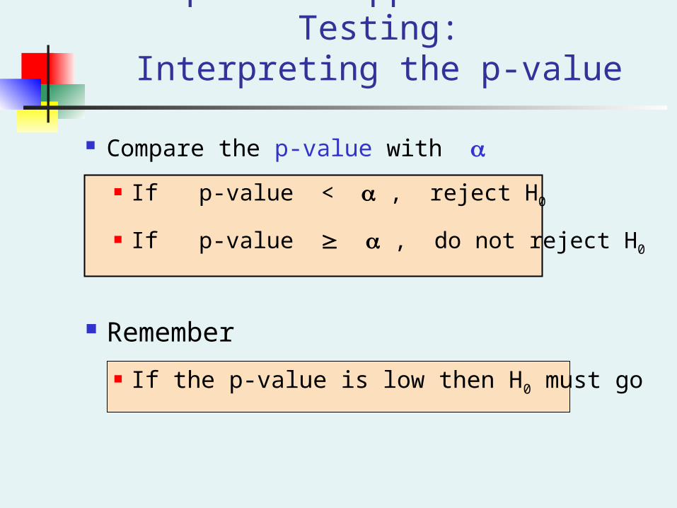
p-Value Approach to Testing:Interpreting the p-value
Compare the p-value with
If p-value < , reject H0
If p-value , do not reject H0
Remember
If the p-value is low then H0 must go
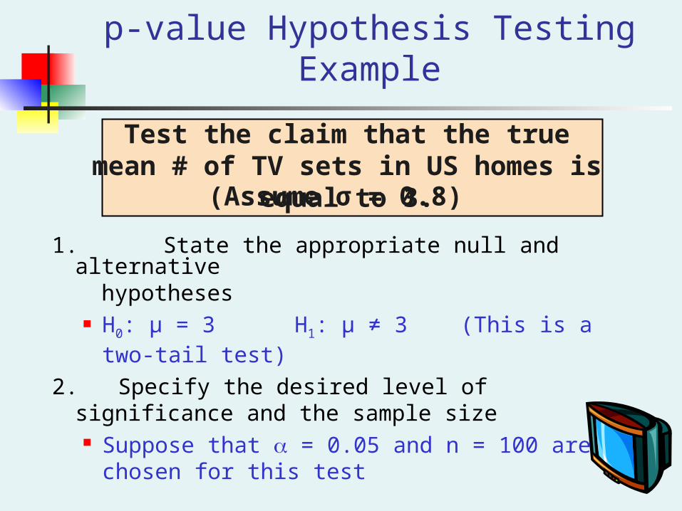
p-value Hypothesis Testing Example
Test the claim that the true mean # of TV sets in US homes is equal to 3.
(Assume σ = 0.8)
1. State the appropriate null and alternative hypotheses
H0: μ = 3 H1: μ ≠ 3 (This is a two-tail test)
2. Specify the desired level of significance and the sample size Suppose that = 0.05 and n = 100 are chosen
for this test
2.0.08
.16
100
0.832.84
n
σμX
STATZ
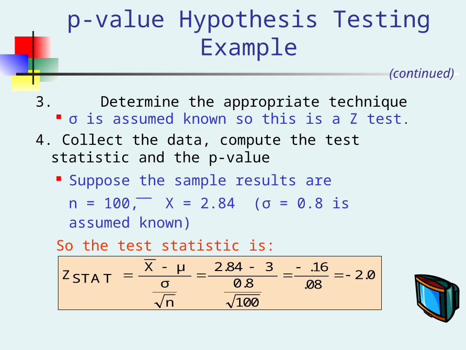
p-value Hypothesis Testing Example
3. Determine the appropriate technique σ is assumed known so this is a Z test.
4. Collect the data, compute the test statistic and the p-value Suppose the sample results are
n = 100, X = 2.84 (σ = 0.8 is assumed known)
So the test statistic is:
(continued)
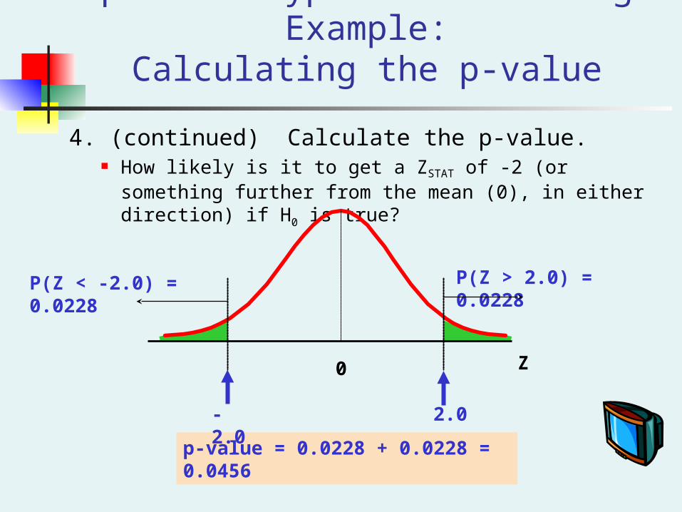
p-Value Hypothesis Testing Example:Calculating the p-value
4. (continued) Calculate the p-value. How likely is it to get a ZSTAT of -2 (or something further from the
mean (0), in either direction) if H0 is true?
p-value = 0.0228 + 0.0228 = 0.0456
P(Z < -2.0) = 0.0228
0
-2.0
Z
2.0
P(Z > 2.0) = 0.0228
5. Is the p-value < α? Since p-value = 0.0456 < α = 0.05 Reject H0
5. (continued) State the managerial conclusion in the context of the situation.
There is sufficient evidence to conclude the average number of TVs in US homes is not equal to 3.
p-value Hypothesis Testing Example
(continued)
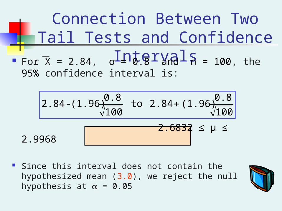
Connection Between Two Tail Tests and Confidence Intervals
For X = 2.84, σ = 0.8 and n = 100, the 95% confidence interval is:
2.6832 ≤ μ ≤ 2.9968
Since this interval does not contain the hypothesized mean (3.0), we reject the null hypothesis at = 0.05
100
0.8 (1.96) 2.84 to
100
0.8 (1.96) - 2.84
Hypothesis Testing: σ Unknown
If the population standard deviation is unknown, you instead use the sample standard deviation S.
Because of this change, you use the t distribution instead of the Z distribution to test the null hypothesis about the mean.
When using the t distribution you must assume the population you are sampling from follows a normal distribution.
All other steps, concepts, and conclusions are the same.

t Test of Hypothesis for the Mean (σ Unknown)
The test statistic is:
n
SμX
STATt
Hypothesis Tests for
σ Known σ Unknown Known Unknown(Z test) (t test)
t Test of Hypothesis for the Mean (σ Unknown)
Convert sample statistic ( ) to a tSTAT test statistic
The test statistic is:
n
SμX
STATt
Hypothesis Tests for
σ Known σ Unknown Known Unknown(Z test) (t test)
X
The test statistic is:
n
SμX
STATt
Hypothesis Tests for
σ Known σ Unknown Known Unknown(Z test) (t test)
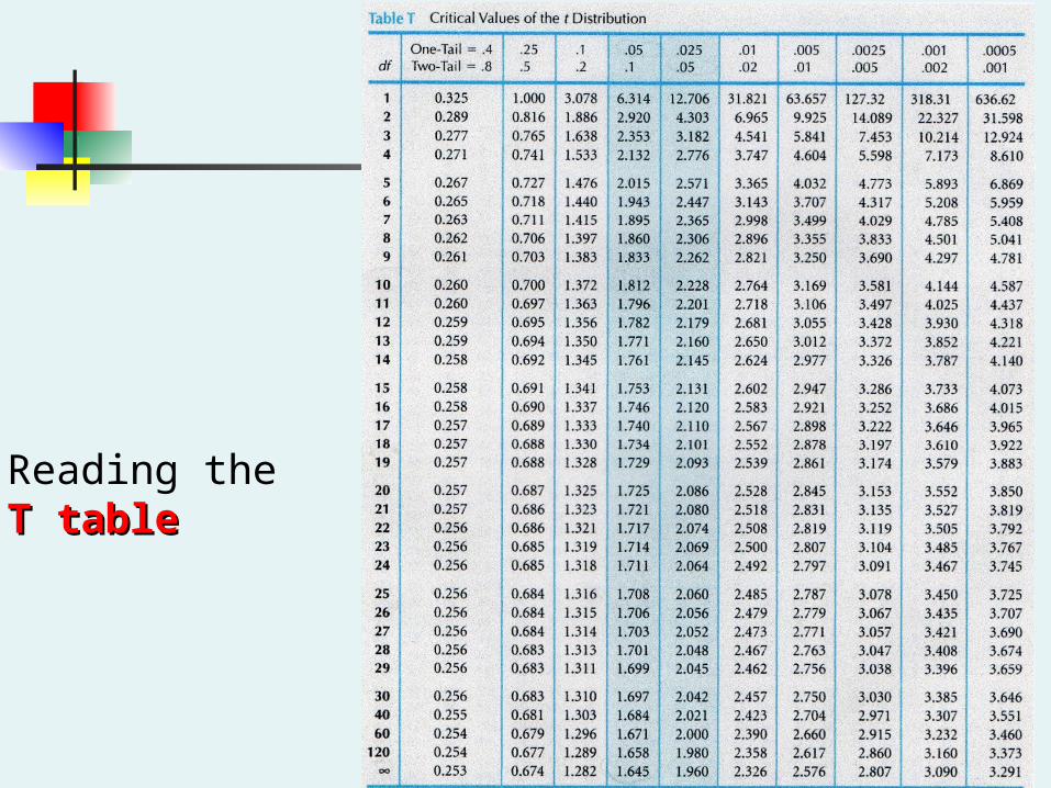
Reading the T tableT table
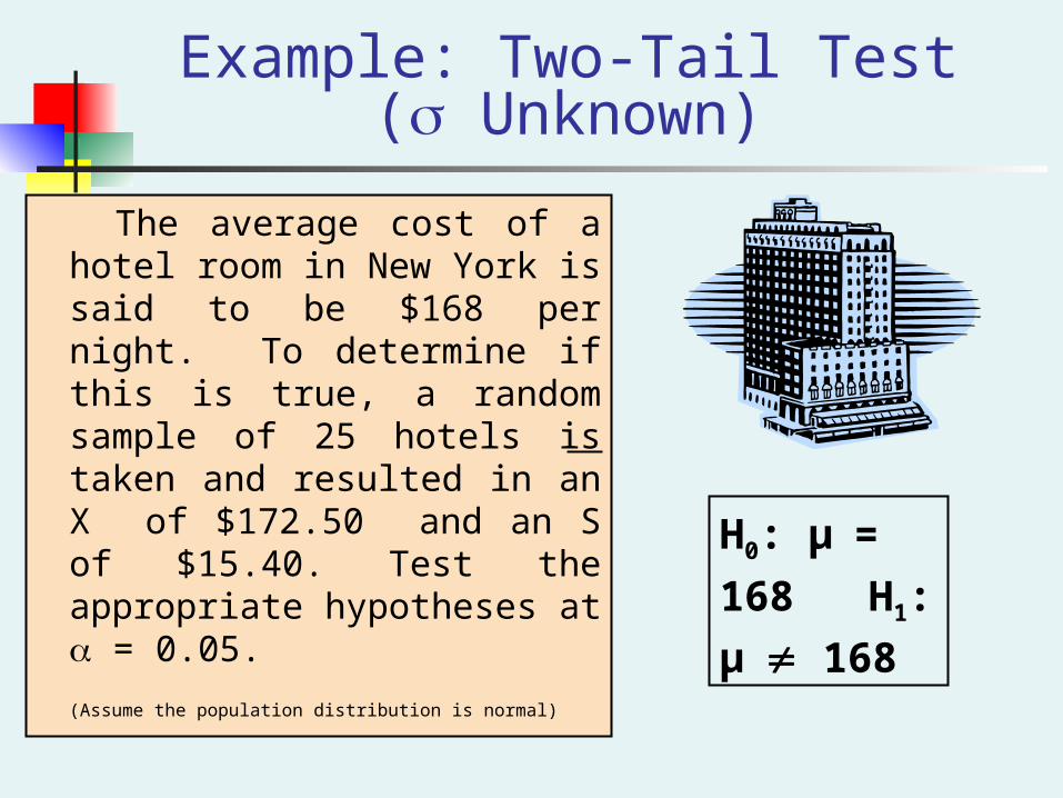
Example: Two-Tail Test( Unknown)
The average cost of a hotel room in New York is said to be $168 per night. To determine if this is true, a random sample of 25 hotels is taken and resulted in an X of $172.50 and an S of $15.40. Test the appropriate hypotheses at = 0.05.
(Assume the population distribution is normal)
H0: μ=
168 H1:
μ 168
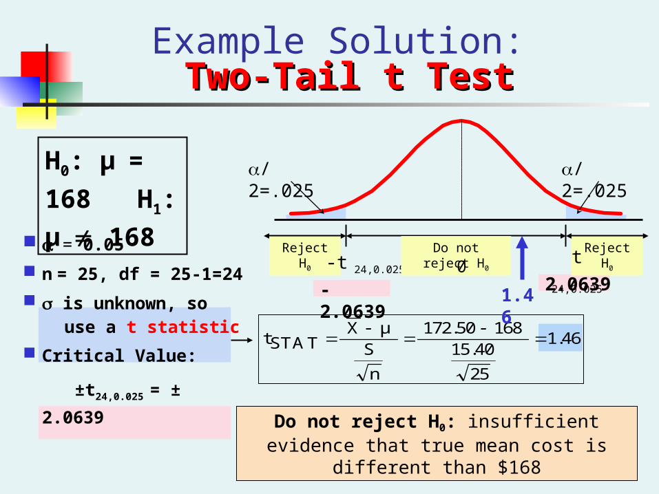
= 0.05
n = 25, df = 25-1=24
is unknown, so use a t statistic
Critical Value:
±t24,0.025 = ± 2.0639
Example Solution: Two-Tail t TestTwo-Tail t Test
Do not reject H0: insufficient evidence that true mean cost is different than $168
Reject H0Reject H0
/2=.025
-t 24,0.025
Do not reject H0
0
/2=.025
-2.0639 2.0639
1.46
25
15.40168172.50
n
SμX
STATt
1.46
H0: μ=
168 H1:
μ 168t 24,0.025
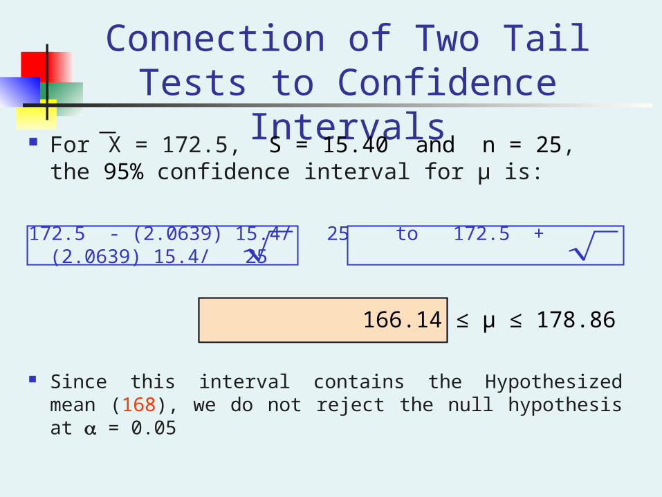
Connection of Two Tail Tests to Confidence Intervals
For X = 172.5, S = 15.40 and n = 25, the 95% confidence interval for µ is:
172.5 - (2.0639) 15.4/ 25 to 172.5 + (2.0639) 15.4/ 25
166.14 ≤ μ ≤ 178.86
Since this interval contains the Hypothesized mean (168), we do not reject the null hypothesis at = 0.05
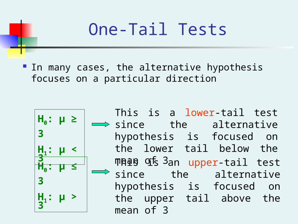
One-Tail Tests
In many cases, the alternative hypothesis focuses on a particular direction
H0: μ ≥ 3
H1: μ < 3
H0: μ ≤ 3
H1: μ > 3
This is a lower-tail test since the alternative hypothesis is focused on the lower tail below the mean of 3
This is an upper-tail test since the alternative hypothesis is focused on the upper tail above the mean of 3
Reject H0 Do not reject H0
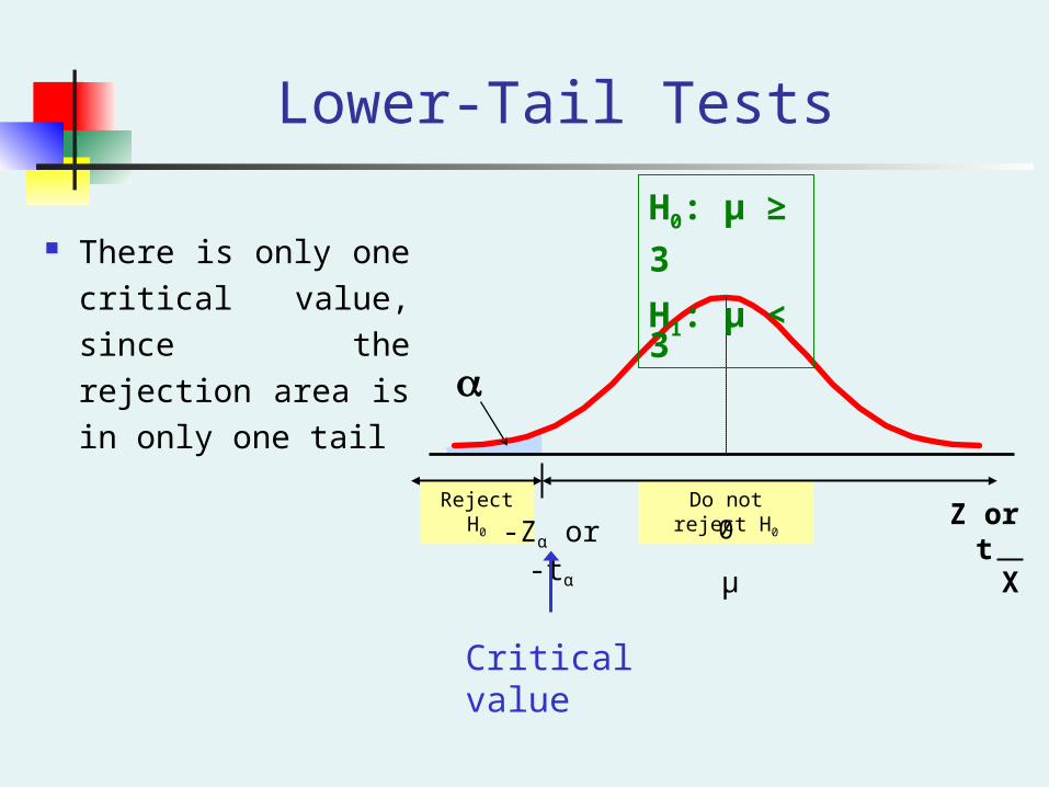
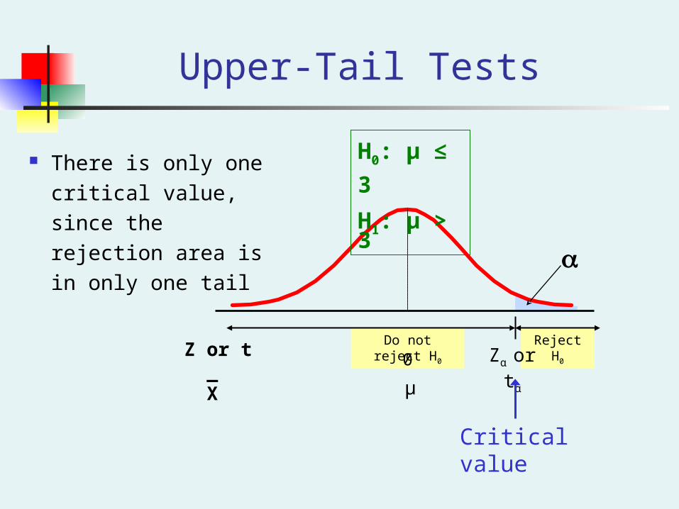
There is only one
critical value, since
the rejection area is
in only one tail
Lower-Tail Tests
-Zα or -tα 0
μ
H0: μ ≥ 3
H1: μ < 3
Z or t
X
Critical value
Reject H0Do not reject H0
Upper-Tail Tests
Zα or tα0
μ
H0: μ ≤ 3
H1: μ > 3
There is only one
critical value, since
the rejection area is
in only one tail
Critical value
Z or t
X_
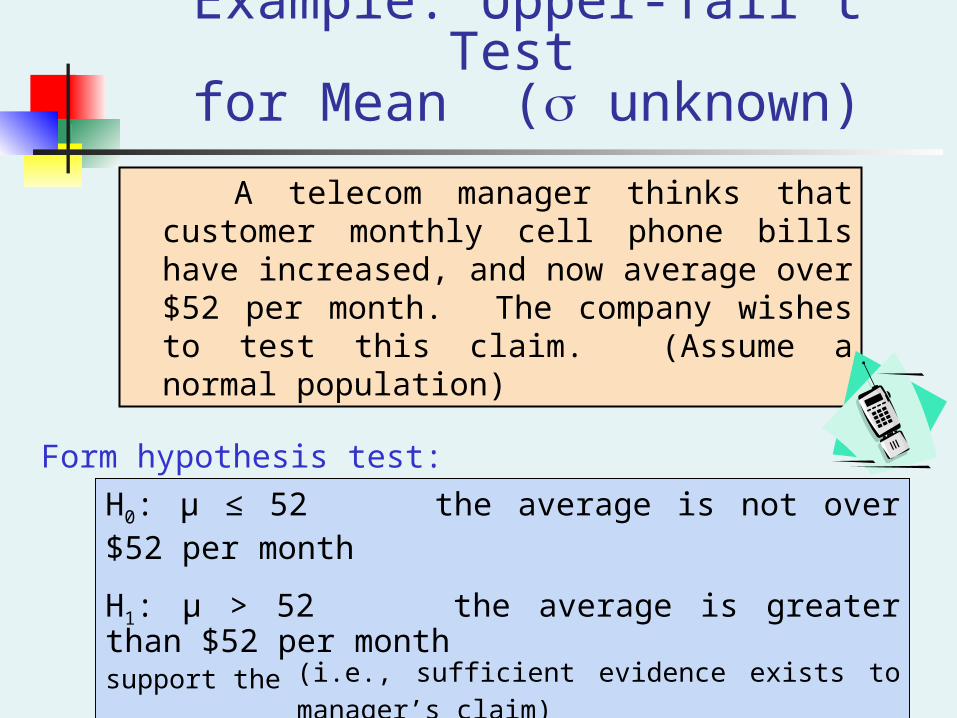
Example: Upper-Tail t Test for Mean ( unknown)
A telecom manager thinks that customer monthly cell phone bills have increased, and now average over $52 per month. The company wishes to test this claim. (Assume a normal population)
H0: μ ≤ 52 the average is not over $52 per month
H1: μ > 52 the average is greater than $52 per month(i.e., sufficient evidence exists to support the manager’s claim)
Form hypothesis test:
Reject H0Do not reject H0
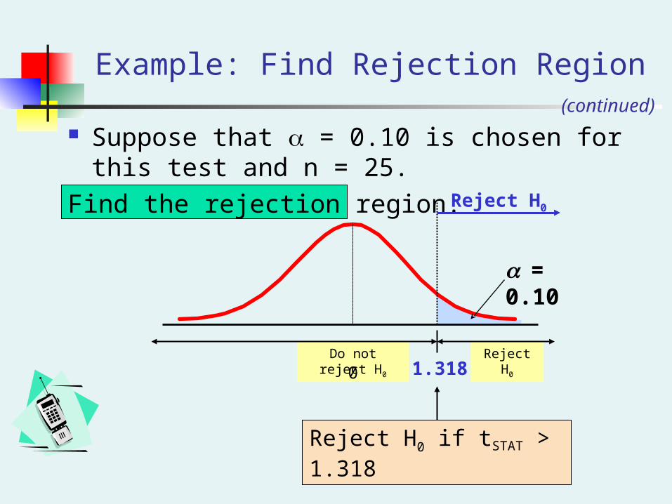
Suppose that = 0.10 is chosen for this test and n = 25.
Find the rejection region:
= 0.10
1.3180
Reject H0
Reject H0 if tSTAT > 1.318
Example: Find Rejection Region(continued)

Obtain sample and compute the test statistic
Suppose a sample is taken with the following results: n = 25, X = 53.1, and S = 10
Then the test statistic is:
0.55
25
105253.1
n
SμX
tSTAT
Example: Test Statistic(continued)
Reject H0Do not reject H0
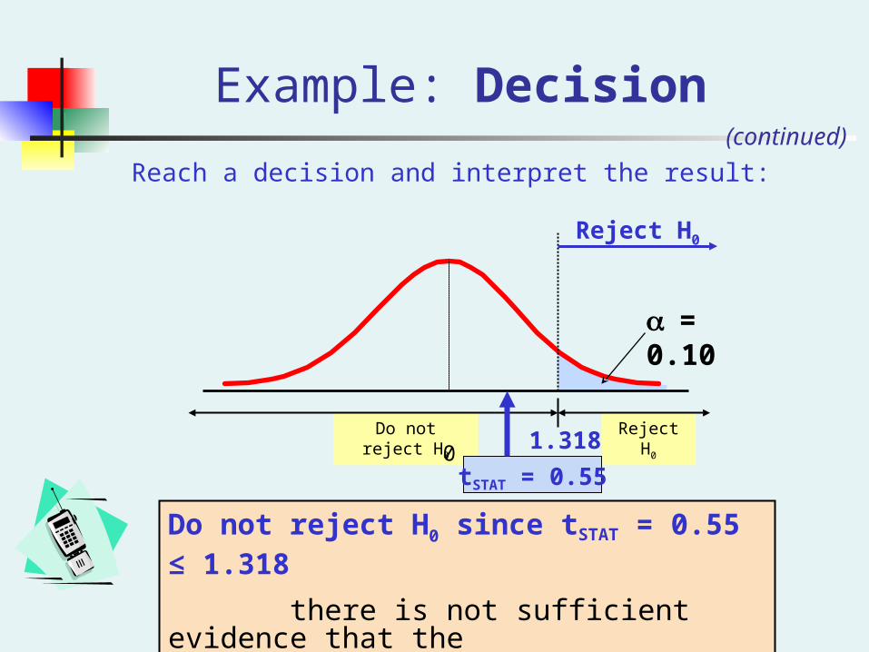
Example: Decision
= 0.10
1.3180
Reject H0
Do not reject H0 since tSTAT = 0.55 ≤ 1.318
there is not sufficient evidence that the mean bill is over $52
tSTAT = 0.55
Reach a decision and interpret the result:(continued)
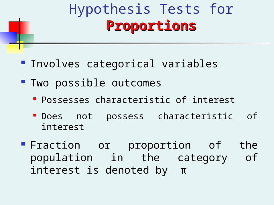
Hypothesis Tests for ProportionsProportions
Involves categorical variables
Two possible outcomes Possesses characteristic of interest
Does not possess characteristic of interest
Fraction or proportion of the population in the category of interest is denoted by π
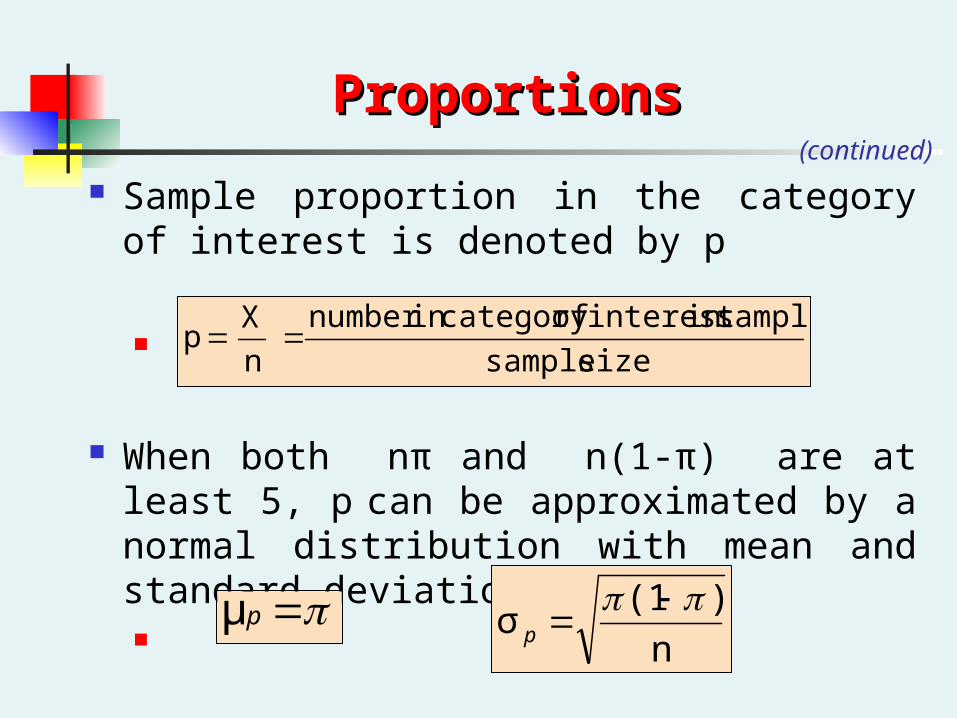
ProportionsProportions
Sample proportion in the category of interest is denoted by p
When both nπ and n(1-π) are at least 5, p can be approximated by a normal distribution with mean and standard deviation
sizesample
sampleininterest ofcategory in number
n
Xp
pμn
)(1σ
p
(continued)
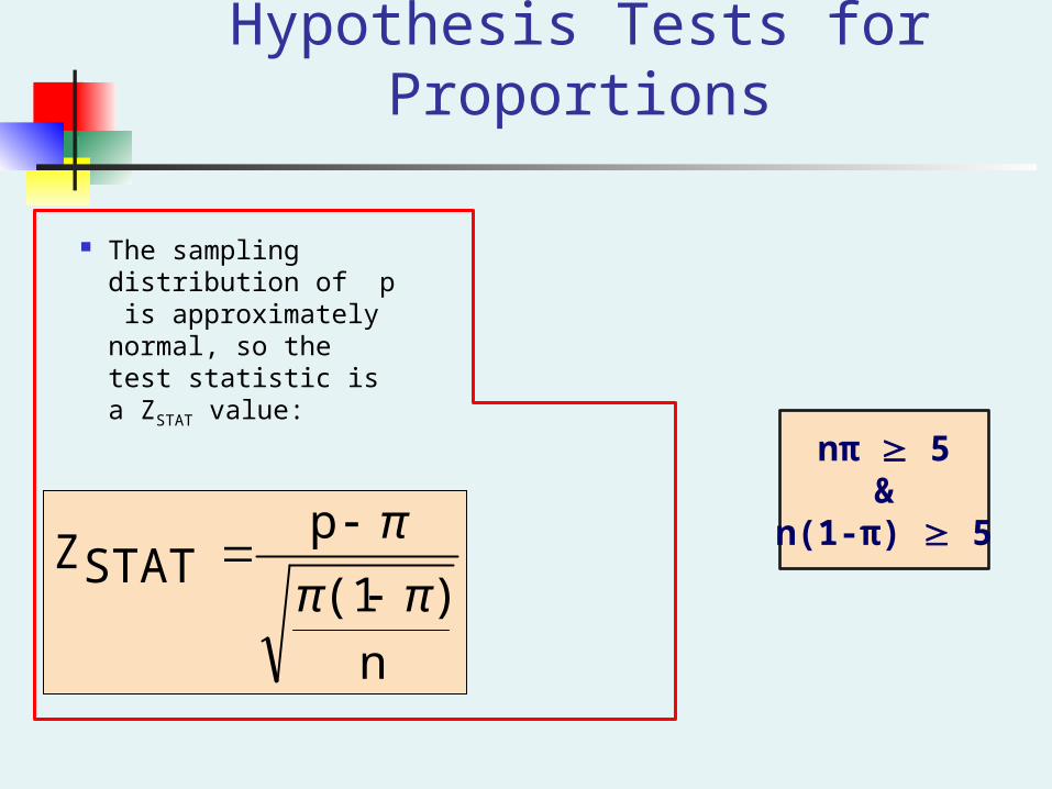
The sampling distribution of p is approximately normal, so the test statistic is a ZSTAT value:
Hypothesis Tests for Proportions
n
)(1
pSTATZ
ππ
π
nπ 5&
n(1-π) 5
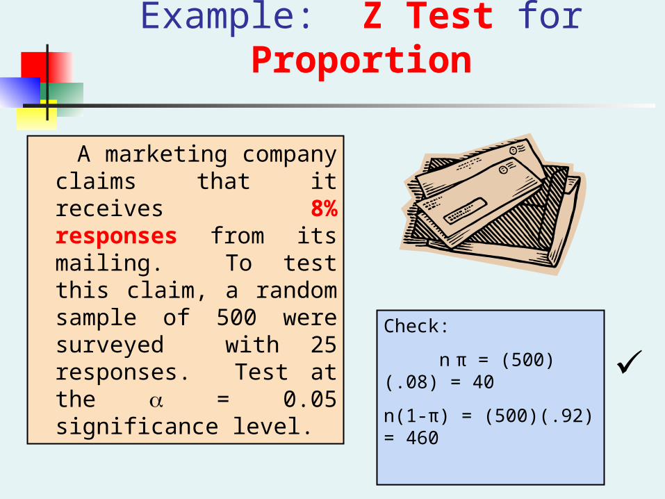
Example: Z Test for Proportion
A marketing company claims that it receives 8% responses from its mailing. To test this claim, a random sample of 500 were surveyed with 25 responses. Test at the = 0.05 significance level.
Check:
n π = (500)(.08) = 40
n(1-π) = (500)(.92) = 460
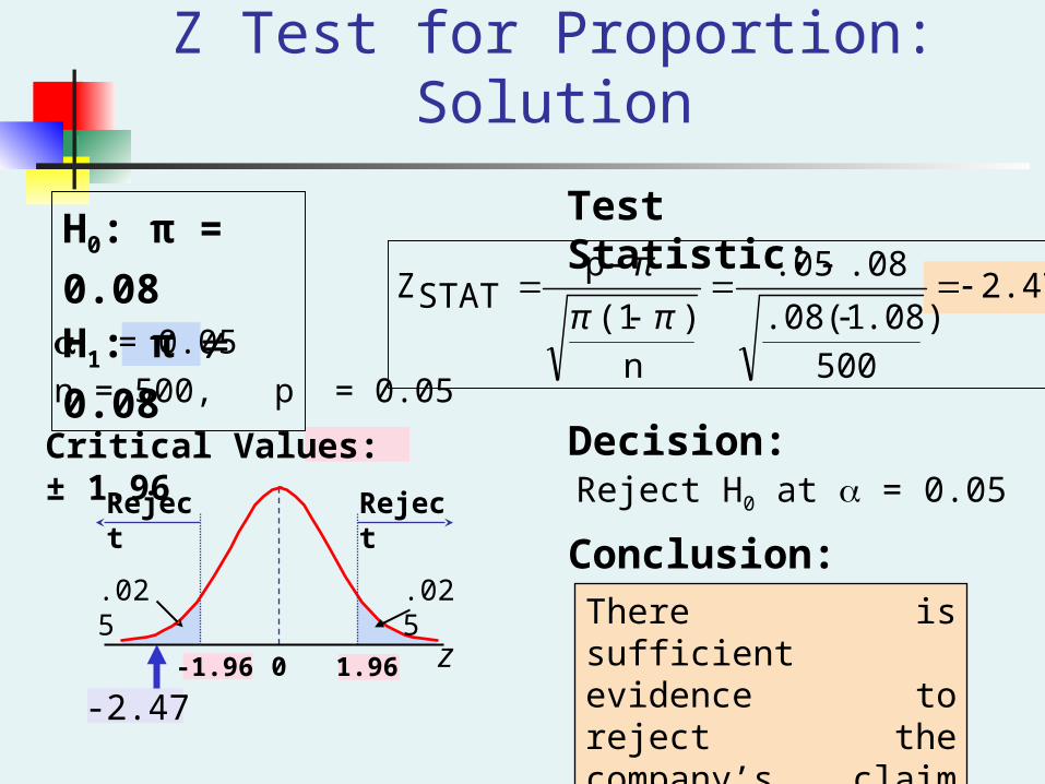
Z Test for Proportion: Solution
= 0.05
n = 500, p = 0.05
Reject H0 at = 0.05
H0: π = 0.08
H1: π
0.08
Critical Values: ± 1.96
Test Statistic:
Decision:
Conclusion:
z0
Reject Reject
.025.025
1.96
-2.47
There is sufficient evidence to reject the company’s claim of 8% response rate.
2.47
500
.08).08(1
.08.05
n
)(1
pSTATZ
ππ
π
-1.96
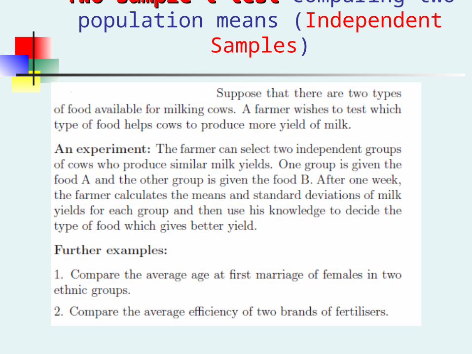
Two-sample t-test Two-sample t-test comparing two population means (Independent Samples)
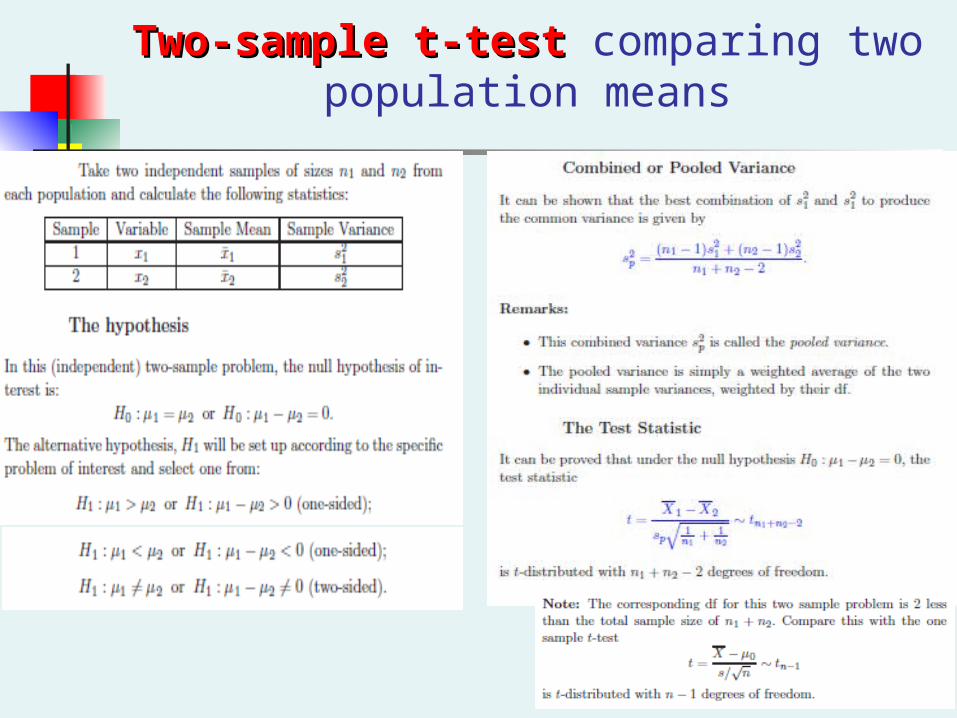
Two-sample t-test Two-sample t-test comparing two population means
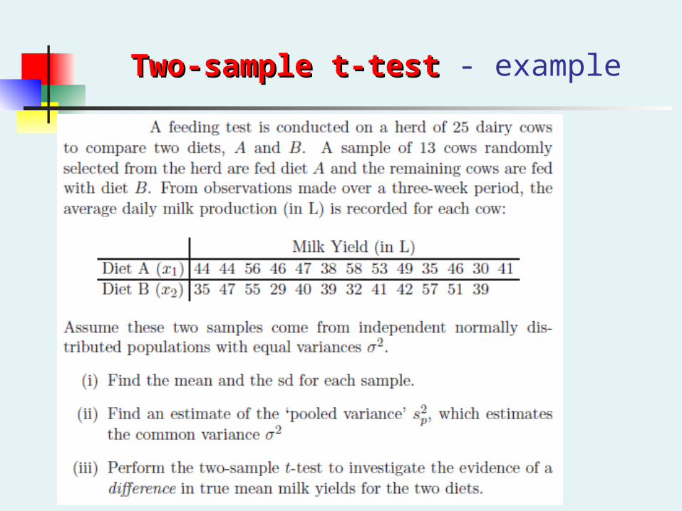
Two-sample t-test Two-sample t-test - example
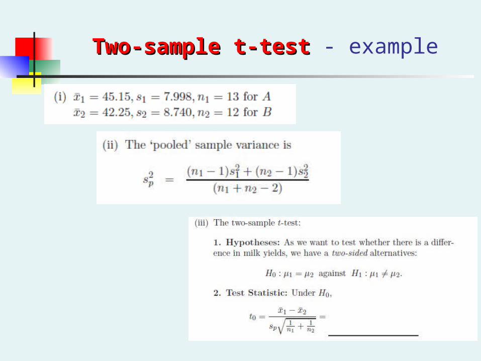
Two-sample t-test Two-sample t-test - example
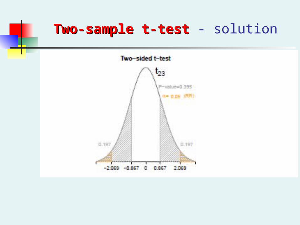
Two-sample t-test Two-sample t-test - solution
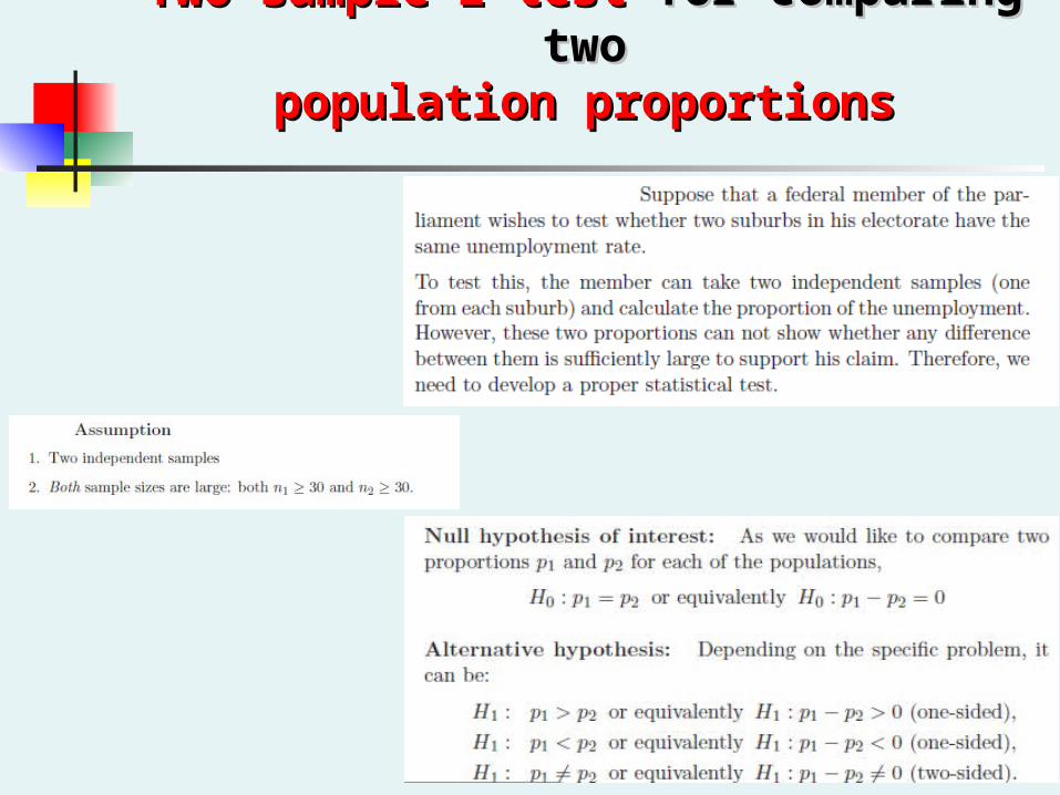
Two-sample z-test Two-sample z-test for comparing twofor comparing twopopulation proportionspopulation proportions
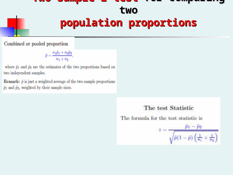
Two-sample z-test Two-sample z-test for comparing twofor comparing twopopulation proportionspopulation proportions

Practice ProblemPractice Problem
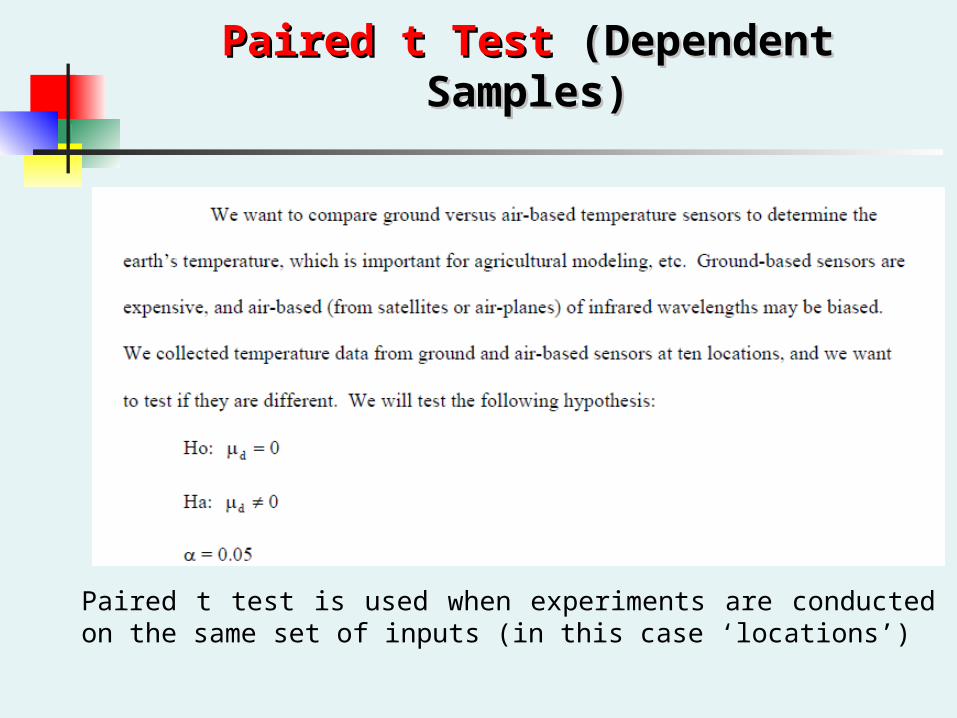
Paired t Test Paired t Test (Dependent Samples)(Dependent Samples)
Paired t test is used when experiments are conducted on the same set of inputs (in this case ‘locations’)
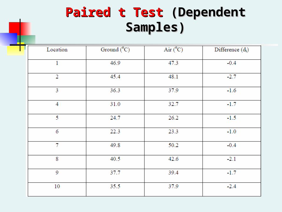
Paired t Test Paired t Test (Dependent Samples)(Dependent Samples)
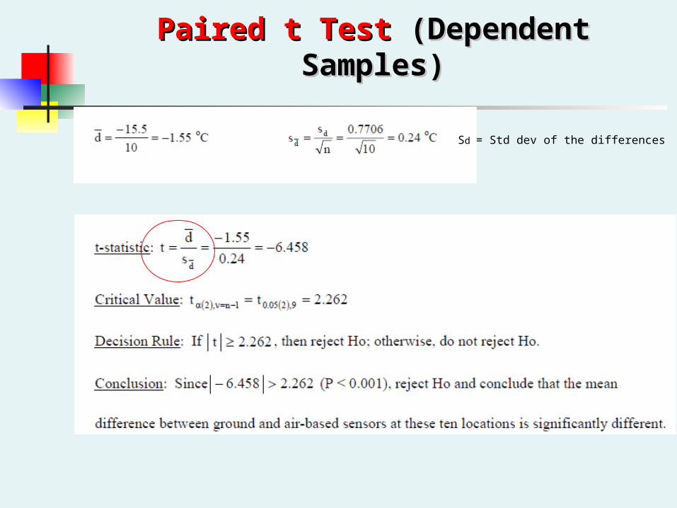
Paired t Test Paired t Test (Dependent Samples)(Dependent Samples)
Sd = Std dev of the differences

Tests for Variances Tests for Variances -Chi-squaredChi-squared-F-testF-test

Chi-squared Chi-squared distributiondistribution
The chi-squared distribution (also chi-square or χ²-distribution) with k (or sometimes ‘df’) degrees of freedom is the distribution of a sum of the squares of k independent standard normal random variables.
If Z1, ..., Zk are independent, standard normal random variables, then the sum of their squares,
is distributed according to the chi-squared distribution with k degrees of freedom. This is usually denoted as
Use: It helps us understand the relationship between categorical variables like age, sex, year etc.
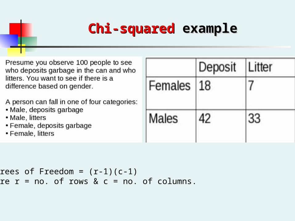
Chi-squared Chi-squared exampleexample
Degrees of Freedom = (r-1)(c-1)Where r = no. of rows & c = no. of columns.
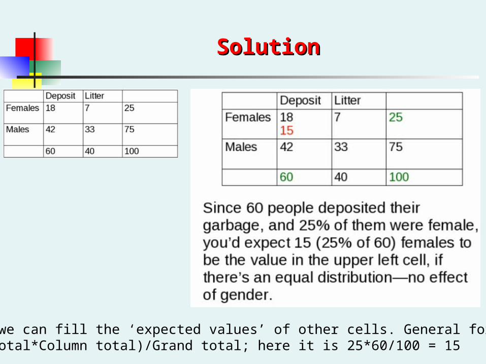
SolutionSolution
Similarly, we can fill the ‘expected values’ of other cells. General formula isEV = (Row Total*Column total)/Grand total; here it is 25*60/100 = 15
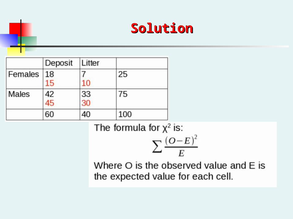
SolutionSolution
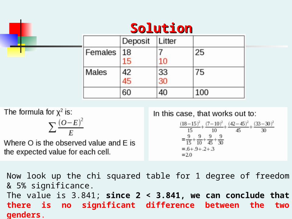
SolutionSolution
Now look up the chi squared table for 1 degree of freedom & 5% significance. The value is 3.841; since 2 < 3.841, we can conclude that there is no significant difference between the two genders.
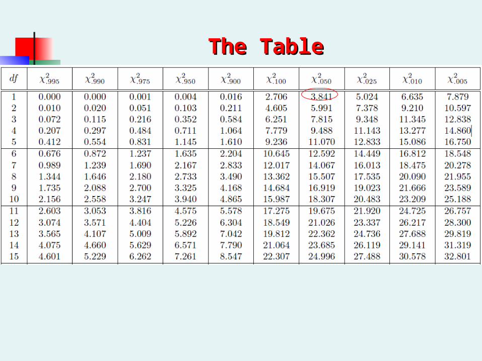
The TableThe Table
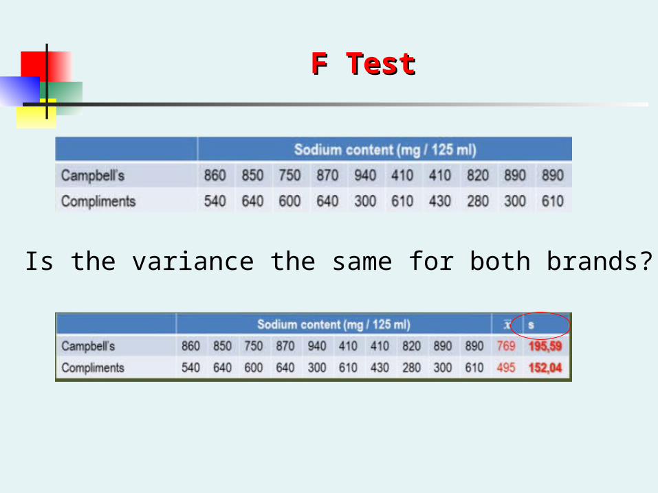
F TestF Test
Is the variance the same for both brands?
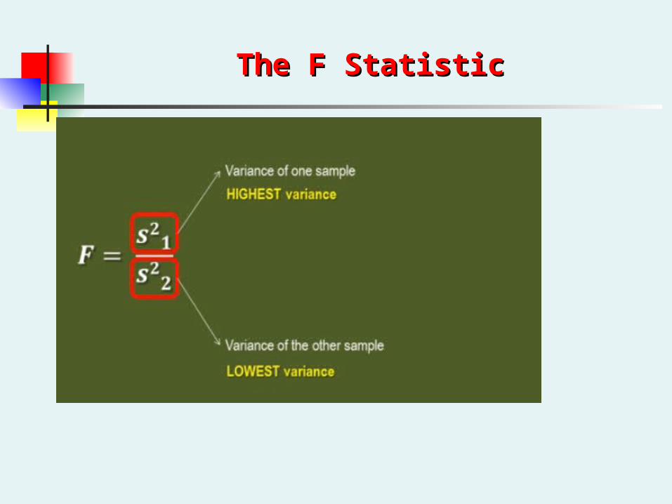
The F StatisticThe F Statistic

The F TableThe F Table
There is one table for each level of significance!DF in Numerator (n-1)
DF in Denominator(n-1)
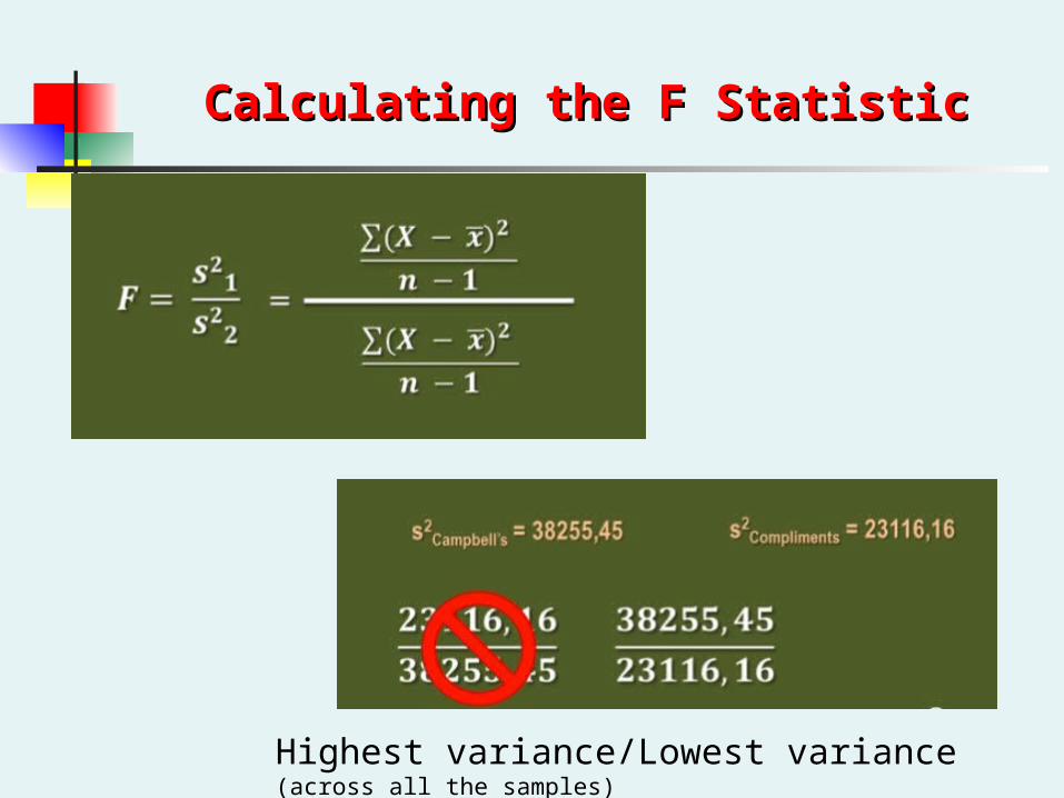
Calculating the F StatisticCalculating the F Statistic
Highest variance/Lowest variance(across all the samples)
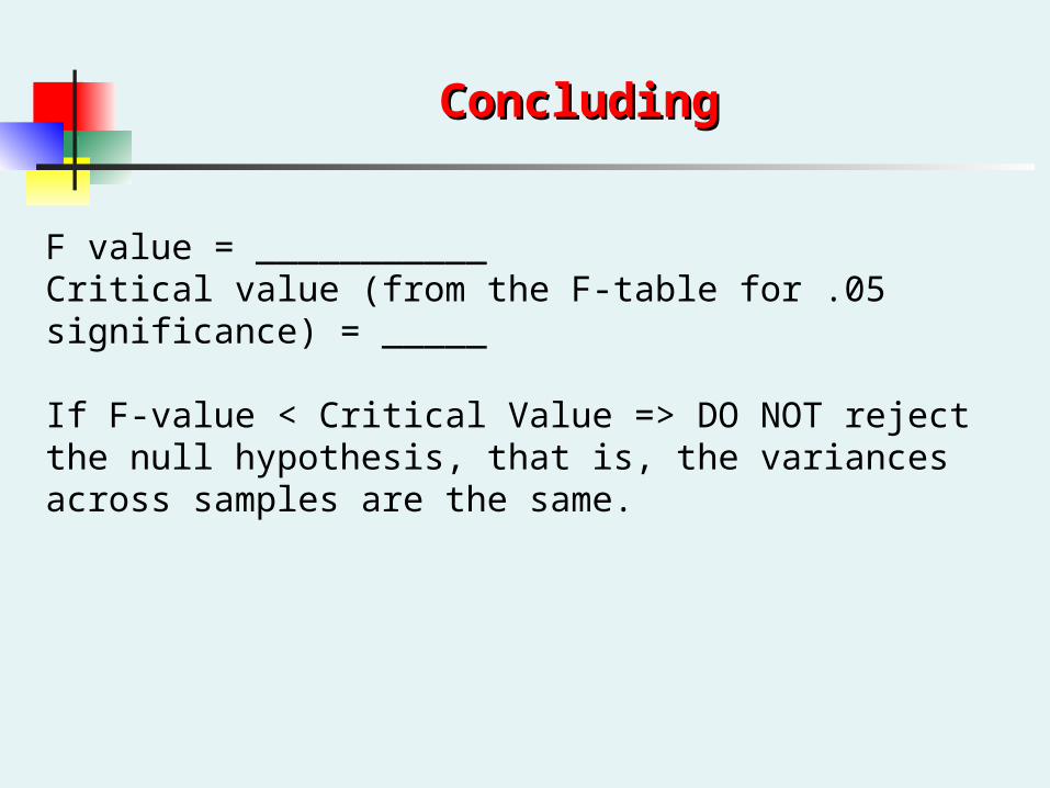
ConcludingConcluding
F value = ___________Critical value (from the F-table for .05 significance) = _____
If F-value < Critical Value => DO NOT reject the null hypothesis, that is, the variances across samples are the same.

Thank Thank youyou!!