1

Hunting for Snarks in Quantum Mechanics

David Hestenesa

aPhysics Department, Arizona State University, Tempe, Arizona 85287.

Abstract. A long-standing debate over the interpretation of quantum mechanics has centered on the meaning of Schroedinger’s wave function ψ for an electron. Broadly speaking, there are two major opposing schools. On the one side, the Copenhagen school (led by Bohr, Heisenberg and Pauli) holds that ψ provides a complete description of a single electron state; hence the probability interpretation of ψψ* expresses an irreducible uncertainty in electron behavior that is intrinsic in nature. On the other side, the realist school (led by Einstein, de Broglie, Bohm and Jaynes) holds that ψ represents a statistical ensemble of possible electron states; hence it is an incomplete description of a single electron state. I contend that the debaters have overlooked crucial facts about the electron revealed by Dirac theory. In particular, analysis of electron zitterbewegung (first noticed by Schroedinger) opens a window to particle substructure in quantum mechanics that explains the physical significance of the complex phase factor in ψ. This led to a testable model for particle substructure with surprising support by recent experimental evidence. If the explanation is upheld by further research, it will resolve the debate in favor of the realist school. I give details. The perils of research on the foundations of quantum mechanics have been foreseen by Lewis Carroll in The Hunting of the Snark!

Keywords: EPR, spacetime algebra, zitterbewegung, Dirac equation, Bohm, Jaynes. PACS: 03.65.-w

1. INTRODUCTION TO SNARK HUNTING

Snark hunting is a danger to your scientific career. A snark hunt is a high stakes search for a hypothesized but yet undiscovered entity or process –– a snark! The hunt is long and demanding; the outcome uncertain and stark. If the hunter succeeds in bagging a real snark, the reward is scientific fame, even a Nobel prize! But beware! The snark may turn out to be a boojum, whereupon the hunter sinks into scientific oblivion or even scorn!

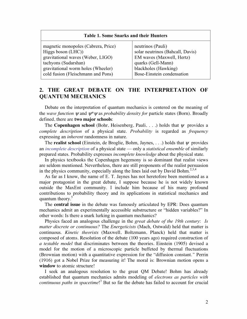
Table 1 lists some famous snarks and their hunters. All the hunts have been strenuous and long, typically consuming decades. I reckon about half the outcomes are boojums, but I leave that for others to decide. Some readers might like to see string theory on the list, but it doesn’t pass the Pauli snark test for a plausible scientific conjecture: “Why it isn’t even wrong!”

Einstein was the greatest snark hunter of all, with several successful hunts under his belt. When queried about his success at sniffing out a snark he explained: “I have a good nose!” His sniffs of quantum mechanics suggested “something is rotten in Denmark.” Whereupon, in the landmark EPR paper,1 he inaugurated what may be the most audacious (some would say “futile”) snark hunt in history. This paper is a report on recent developments.

2

Table 1. Some Snarks and their Hunters

magnetic monopoles (Cabrera, Price) Higgs boson (LHC)) gravitational waves (Weber, LIGO) tachyons (Sudarshan) gravitational worm holes (Wheeler) cold fusion (Fleischmann and Pons)

neutrinos (Pauli) solar neutrinos (Bahcall, Davis) EM waves (Maxwell, Hertz) quarks (Gell-Mann) blackholes (Hawking) Bose-Einstein condensation

2. THE GREAT DEBATE ON THE INTERPRETATION OF QUANTUM MECHANICS

Debate on the interpretation of quantum mechanics is centered on the meaning of the wave function ψ and ψ*ψ as probability density for particle states (Born). Broadly defined, there are two major schools:

The Copenhagen school (Bohr, Heisenberg, Pauli, . . .) holds that ψ provides a complete description of a physical state. Probability is regarded as frequency expressing an inherent randomness in nature.

The realist school (Einstein, de Broglie, Bohm, Jaynes, . . .) holds that ψ provides an incomplete description of a physical state –– only a statistical ensemble of similarly prepared states. Probability expresses incomplete knowledge about the physical state.

In physics textbooks the Copenhagen hegemony is so dominant that realist views are seldom mentioned. Nevertheless, there are still proponents of the realist persuasion in the physics community, especially along the lines laid out by David Bohm.2,3,4

As far as I know, the name of E. T. Jaynes has not heretofore been mentioned as a major protagonist in the great debate, I suppose because he is not widely known outside the MaxEnt community. I include him because of his many profound contributions to probability theory and its applications in statistical mechanics and quantum theory.5

The central issue in the debate was famously articulated by EPR: Does quantum mechanics admit an experimentally accessible substructure or “hidden variables?” In other words: Is there a snark lurking in quantum mechanics?

Physics faced an analogous challenge in the great debate of the 19th century: Is matter discrete or continuous? The Energeticists (Mach, Ostwald) held that matter is continuous. Kinetic theorists (Maxwell, Boltzmann, Planck) held that matter is composed of atoms. Resolution of the debate (100 years ago) required construction of a testable model that discriminates between the theories. Einstein (1905) devised a model for the motion of a microscopic particle buffeted by thermal fluctuations (Brownian motion) with a quantitative expression for the “diffusion constant.” Perrin (1916) got a Nobel Prize for measuring it! The moral is: Brownian motion opens a window to atomic structure!

I seek an analogous resolution to the great QM Debate! Bohm has already established that quantum mechanics admits modeling of electrons as particles with continuous paths in spacetime!3 But so far the debate has failed to account for crucial

3

facts about spin and zitterbewegung in Dirac electron theory! I claim that spin and zitterbewegung provide a window to particle substructure in quantum mechanics. My purpose here is to open that window with a particle model of the substructure that has new experimental implications.

3. SPACETIME ALGEBRA

Spacetime Algebra (STA) is an essential tool for explicating the geometric structure of spin and complex numbers in the Dirac Equation. It has been explained and applied at length elsewhere,6,7 so only a brief review is needed here. STA can be generated by an orthonormal basis of vectors !µ satisfying the product rule:

!

0

2= 1, !

k

2= "1 (k = 1,2,3) . (1)

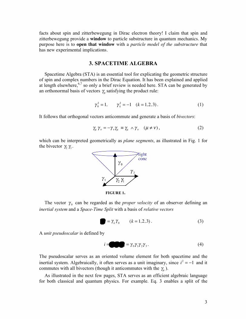
It follows that orthogonal vectors anticommute and generate a basis of bivectors: !µ ! " = #! "!µ $ !µ % ! " (µ & ") , (2) which can be interpreted geometrically as plane segments, as illustrated in Fig. 1 for the bivector !

2!1.

The vector !0 can be regarded as the proper velocity of an observer defining an

inertial system and a Space-Time Split with a basis of relative vectors !

k= "

k"0

(k = 1,2,3) . (3) A unit pseudoscalar is defined by i = !

1!2!3= "

0"1"2"3. (4)

The pseudoscalar serves as an oriented volume element for both spacetime and the inertial system. Algebraically, it often serves as a unit imaginary, since i2 = !1 and it commutes with all bivectors (though it anticommutes with the !µ ).

As illustrated in the next few pages, STA serves as an efficient algebraic language for both classical and quantum physics. For example. Eq. 3 enables a split of the

FIGURE 1.

4

electromagnetic field F, which is a bivector quantity, into electric and magnetic fields (units c = 1): F = 1

2F

!µ"µ# "! = F0k$k + 1

2F

jk$k $ j = E + iB . (5)

The algebraic convenience of representing the complete electromagnetic field as a complex vector has been noted many times, but here the unit imaginary is the unit pseudoscalar so it has a geometric meaning (which, by the way, explains why B is an axial vector, while E is a polar vector in standard vector algebra)6.

Of course, the notation !µ has been chosen to emphasize isomorphism with the Dirac matrices. Thus, the Dirac algebra (over the reals) is a matrix representation of STA, and hence of spacetime geometry; so it has no special significance for spin and quantum mechanics. Matrix representation is simply irrelevant to the geometric function of STA.

Likewise, the !k

are isomorphic to the “Pauli spin matrices,” but they have no special relation to spin, and representation by matrices is irrelevant.

Lorentz rotations without matrices

Any Lorentz rotation can be generated by a rotor R:

! µ " eµ = R! µ

!R . (6) The rotor is called a spin representation and defined by

R !R = 1, Ri = iR, whence R = e

12 B

, !R = e! 12 B , (7)

where B is a bivector.

The rotation can be decomposed into a boost and a spatial rotation by a multiplicative Space-Time Split R = LU, where the boost is given by

e0= R!

0!R = L!

0!L = L

2!0, whence L = (e

0!0)1/2 , (8)

and

U!

0

!U = !0determines the spatial rotation given by

ek!U"

k!U =U#

k#0

!U =U#k!U#

0= !L e

ke0L . (9)

These rotor-generated rotations are readily related to the usual matrix representations, but that is not necessary for applications.

5

Rotor particle mechanics

Let x = x(! ) be the spacetime history of a particle with proper time τ. The particle’s proper velocity

!x = v(! ) is then a unit vector so, according to Eq. 6, its time

evolution can be expressed as a Lorentz rotation v = R!

0

!R , where the rotor R = R(! ) satisfies an equation of motion of the form

dR

d!= !R =

1

2"R . (10)

Differentiating Eq. 7, we find that

! = 2 !R "R = "2R "

!R = " "! , which implies that Ω is a

bivector, so we can regard it as a rotational velocity. Accordingly, the particle acceleration is given by

dv

d!= !v = !R"

0"R + R"

0"!R =

12(#v + v#) = #$ v . (11)

What does the rotor equation of motion buy us? First note that for a particle with

mass m and charge q we can write

! =qm F " m !v = qF # v , (12)

which will be recognized as the classical Lorentz force equation. Thus, the electromagnetic bivector F acts as a rotational velocity for a charged particle. As a practical matter, the rotor equation can be easier to solve than the Lorentz force equation.6

There is more! Identifying the particle velocity with e0= R!

0

!R = v = "x in Eq. 6, we can regard the eµ = eµ (! ) as a comoving frame defined on the particle history. Its equation of motion is then given by

eµ = R!µ

!R " "eµ = #$ eµ . (13) The rotating frame can be regarded as a spinning body with precession determined by Ω. In particular, if we define a spin vector s by

s =!

2e3=!

2R!

3

"R , (14)

then Eq. 12 implies the equation of motion

6

!s =qm F ! s . (15)

This describes spin precession for a magnetic moment with g-factor 2, in agreement with the Dirac equation. In fact, it can be derived as a classical limit of the Dirac equation.6 This gives insight into the origin of the g-factor that helps guide the design of particle models in quantum mechanics below.

As we see next, rotors are spinors, but without the complex numbers of a matrix representation. We conclude, therefore, that real spinors are natural and useful in both classical and quantum theory!

4. REAL QUANTUM MECHANICS WITH STA

When the Dirac equation is translated into STA it takes the form

! µ("µ

# !2!1! $ qAµ

# ) = me#!

0. (16)

I call this the real Dirac equation, because the superfluous complex numbers in the Dirac matrix algebra have been eliminated in favor of objects with geometric meaning. This raises the question of the physical significance of the newly recognized geometric objects. The answer provides an important clue in the snark hunt for deeper meaning in quantum mechanics.

The real wave function in Eq. 16 can be written in the canonical form

! = ("ei# )1

2 R =! (x) , (17) where, as before, R = R(x) is a rotor-valued function, but now it is a rotor field on spacetime. As R defines a Lorentz rotation at each spacetime point x, it follows from Eq. 7 that it is a 6-parameter function –– an insight that is totally missed in the matrix version of the Dirac wave function.

The remaining two parameters in the wave function are the scalars ! = !(x) , usually interpreted as a probability density, and ! = !(x) , for which the physical interpretation is problematic.6 Fortunately, β will not play a role in our considerations here.

It is immediately obvious in Eq. 16 that the role of the unit imaginary in the matrix Dirac equation has been replaced by the bivector i ! "

2"1= i#

3. (18)

In has the property i2 = (!

2!1)2= "1 required for the generator of phase rotations in

the wave function, but, as illustrated in Fig. 1, it is associated with a spacelike plane, so it is the generator of rotations in that plane. This tells us that imaginary numbers in

7

the wave functions of quantum mechanics have a geometric meaning! –– Do we smell a snark?

To make the invariance of the Dirac equation explicit, we express spacetime position as a vector x = !µ x

µ that is independent of the coordinate choice xµ= x ! " µ .

Similarly, we use coordinate derivatives to define the invariant vector derivative with respect to that point by ! = "

x= # µ"µ . Then we can write Eq. 16 in the coordinate

invariant form

!" i! # qA" = me

" $0. (19)

The vector !

0 on the right side of this equation is an arbitrary timelike vector in the

forward light cone not necessarily related to coordinates, though that may be convenient, as we see in examining observables.

Local observables

In the present formulation, the usual Dirac current is defined by

! "

0!! = #v, where v = R"

0!R = e

0(x) . (20)

From Eq. 19 we derive the well known conservation law

! " (# $

0!# ) = ! " (%v) = 0 , (21)

which allows one to interpret the Dirac current as a probability current or proportional to a charge current.

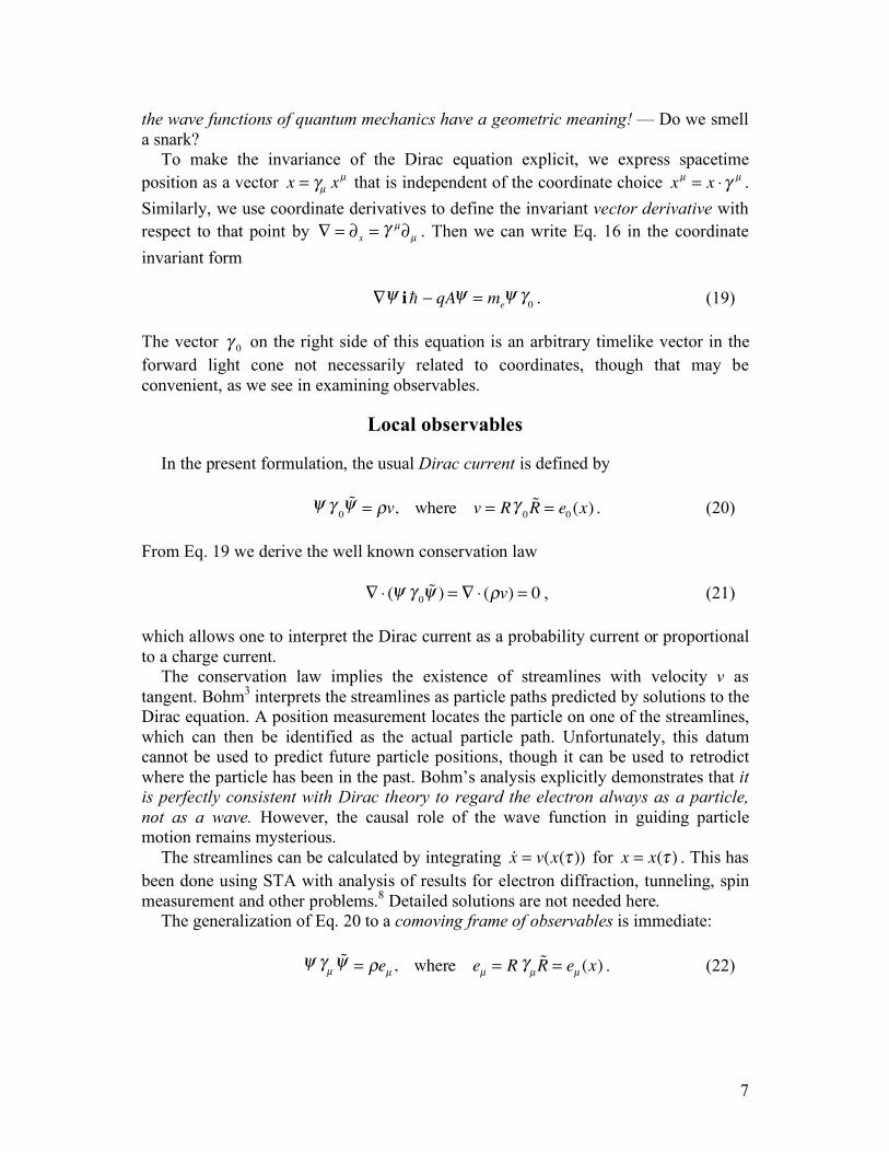
The conservation law implies the existence of streamlines with velocity v as tangent. Bohm3 interprets the streamlines as particle paths predicted by solutions to the Dirac equation. A position measurement locates the particle on one of the streamlines, which can then be identified as the actual particle path. Unfortunately, this datum cannot be used to predict future particle positions, though it can be used to retrodict where the particle has been in the past. Bohm’s analysis explicitly demonstrates that it is perfectly consistent with Dirac theory to regard the electron always as a particle, not as a wave. However, the causal role of the wave function in guiding particle motion remains mysterious.

The streamlines can be calculated by integrating !x = v(x(! )) for x = x(! ) . This has

been done using STA with analysis of results for electron diffraction, tunneling, spin measurement and other problems.8 Detailed solutions are not needed here.

The generalization of Eq. 20 to a comoving frame of observables is immediate:

! "µ!! = #eµ , where eµ = R "

µ!R = eµ (x) . (22)

8

The spin vector s defined by Eq. 14 can be identified as a physical observable in this frame. However, angular momentum is a bivector quantity, so a more appropriate representation of spin is the spin bivector:

S = isv =!

2ie3e0=!

2e2e1=!

2R!

2!1"R =

12R(i!) "R . (23)

This establishes an explicit relation between spin and the generator of phase rotations in the Dirac equation (Eq. 18). The unshakable conclusion is that spin and complex numbers are inseparably related in Dirac theory, hence in all of quantum mechanics! The scent of snark grows stronger!

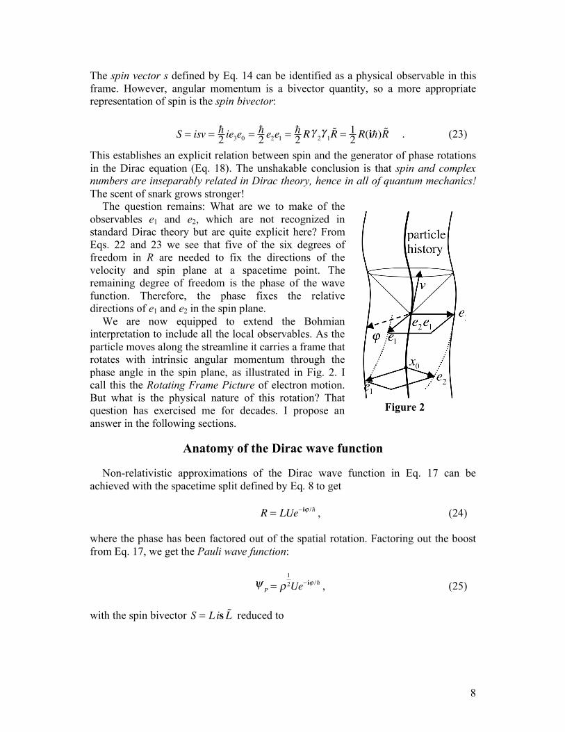
The question remains: What are we to make of the observables e1 and e2, which are not recognized in standard Dirac theory but are quite explicit here? From Eqs. 22 and 23 we see that five of the six degrees of freedom in R are needed to fix the directions of the velocity and spin plane at a spacetime point. The remaining degree of freedom is the phase of the wave function. Therefore, the phase fixes the relative directions of e1 and e2 in the spin plane.

We are now equipped to extend the Bohmian interpretation to include all the local observables. As the particle moves along the streamline it carries a frame that rotates with intrinsic angular momentum through the phase angle in the spin plane, as illustrated in Fig. 2. I call this the Rotating Frame Picture of electron motion. But what is the physical nature of this rotation? That question has exercised me for decades. I propose an answer in the following sections.

Anatomy of the Dirac wave function

Non-relativistic approximations of the Dirac wave function in Eq. 17 can be achieved with the spacetime split defined by Eq. 8 to get R = LUe

! i" /! , (24) where the phase has been factored out of the spatial rotation. Factoring out the boost from Eq. 17, we get the Pauli wave function:

!

P= "

1

2Ue# i$ /! , (25)

with the spin bivector

S = L is !L reduced to

Figure 2

9

is =1

2U i!

3! "U = i

!

2U !

3

"U . (26)

Finally, the U is factored out to get the Schroedinger wave function:

!

S= "

1

2e# i$ /! , (27)

with the unit imaginary given by Eq. 18. This demonstrates explicitly that, when derived as an approximation of the Dirac equation, the Schroedinger equation describes a particle with spin in a fixed direction.

This is a good place to summarize lessons learned from Real Dirac Theory:

• Complex numbers are inseparably related to spin in Dirac theory. Hence spin is essential to interpretation of quantum mechanics even in Schroedinger theory.

• Bilinear observables are geometric consequences of rotational kinematics. Hence, they are as natural in classical mechanics as in quantum mechanics.

• Spin and phase are inseparable kinematic properties of electron motion. Wave function phase is a measure of rotation in the spin plane.

5. MODELING ELECTRON SPIN AND ZITTER

One serious problem remains for interpreting the Dirac equation. If the electron is really a structureless point particle, how does it generate a magnetic moment proportional to its spin? I call this the zitterbewegung problem, after Schroedinger’s original attempt to address it.9 The idea has been clearly articulated by Huang:10

“The well-known Zitterbewegung may be looked upon as a circular motion about the direction of the electron spin with radius equal to the Compton wavelength × 1/2π of the electron. The intrinsic spin of the electron may be looked upon as the orbital angular momentum of this motion. The current produced by the Zitterbewegung is seen to give rise to the intrinsic magnetic moment of the electron.”

Dirac approved the idea soon thereafter,11 so on his authority it has been duly reiterated in textbooks on relativistic quantum mechanics to this day. However, nothing has been made of its staggering theoretical implications:

• Quantum mechanics has a circulating particle substructure that generates the electron’s magnetic moment.

• Wave function phase describes circulating substructure motion. • This motion generates a fluctuating electric field.

If these claims are real physical effects, so that zitterbewegung is more than a colorful metaphor, then we need a testable particle model of the electron with spin and zitterbewegung to explain them.

10

As Einstein advised, our model should be as simple as possible –– but not simpler! The spinning frame picture of observables in Dirac theory tells us what geometric features must be incorporated in the model for consistency with Dirac theory. Let me describe a model that was recently developed to meet these criteria.12 I call it the Zitter Particle Model (ZPM) of the electron. I have adopted the term zitter because zitterbewegung is such a mouthful and the model modifies Schroedinger’s original concept.

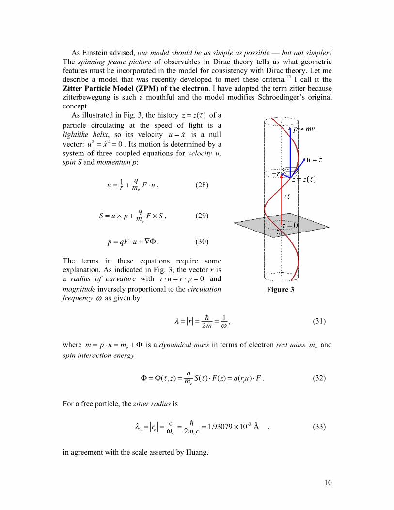
As illustrated in Fig. 3, the history z = z(! ) of a particle circulating at the speed of light is a lightlike helix, so its velocity u = !x is a null vector: u2 = !x2 = 0 . Its motion is determined by a system of three coupled equations for velocity u, spin S and momentum p:

!u = 1r +qme

F !u , (28)

!S = u ! p +qme

F " S , (29)

!p = qF !u +"# . (30)

The terms in these equations require some explanation. As indicated in Fig. 3, the vector r is a radius of curvature with r !u = r ! p = 0 and magnitude inversely proportional to the circulation frequency ! as given by

! = r =!

2m=1

", (31)

where m = p !u = m

e+" is a dynamical mass in terms of electron rest mass m

e and

spin interaction energy

! = !(" , z) =qme

S(" ) #F(z) = q(reu) #F . (32)

For a free particle, the zitter radius is

!e = re=c" e

= !

2mec=1.93079 #10-3 Å , (33)

in agreement with the scale asserted by Huang.

Figure 3

11

A noteworthy feature of the ZPM is the fact that the zitter spin must be a null bivector S = m

ereu = r

e! (m

eu) . (34)

It took me a long time to realize this fact as I expected a spacelike spin as in the Dirac theory. However, the relation to Dirac is more subtle, as we see below.

Rotor version of the ZPM

In a now familiar way, the three equations of motion for the ZPM can be reduced to the single rotor Eq. 10 by introducing a comoving frame

eµ = R!µ

!R . The frame is related to the observables by

u = e

0+ e

2= R(!

0+ !

2) !R , (35)

S =!

2ue

1=!

2(e0e1+ e

2e1) , (36)

p = m

eu ! me

2= m

ee0! "e

21. (37)

The dynamics is encoded in the rotational velocity

! =qm

eF +"e

2e1+ au . (38)

We have already seen that the first term on the right generates the Lorentz force and spin precession consistent with Dirac theory. The second term shows the zitter frequency

! = !" as an “internal” rotation rate in the e

2e1 plane in close analogy to

Dirac theory, so its integral ! is analogous to the quantum mechanical phase, and the zitter energy of this internal motion has the suggestive form

!

2! = m = m

e+" . (39)

The last term determines the flow of energy in and out of the zitter. The explicit form of the vector a is a bit complicated, but it will not be needed here.

To separate the zitter circulation from the motion of its center, we define the average particle velocity over a zitter period by v = u = e

0. (40)

12

This vector is the analog of the Dirac current velocity, and it defines an instantaneous rest system for the zitter electron wherein the point charge can be pictured as circulating about a fixed point.

Now we can get insight into the physical significance of the null spin by performing a spacetime split with respect to v exactly as defined in Section 3. The split can be enacted by S = v2S = v(v !S + v " S) . From Eq. 36 we obtain

v ! S =!

2e0e2e1" is , (41)

where s is identical to the spin vector defined by Eq. 14. Likewise, from Eq. 36 with radius vector r

e! "#

ee1we find

v(v !S) =!

2ve1= m

ev!

2me

e1= "m

evr

e# m

ere=!

2r̂ . (42)

These last two equations combine to give us an explicit expression for the spin split: S = m

evr + S = m

ere+ is , (43)

where the mean spin over a zitter period is S ! v(v " S) = isv ! is . The relative vector rerotates with zitter frequency, so its mean is zero. With a rest frame split of the electromagnetic field F = v(v !F + v " F) = E + iB ,

we can express the spin interaction energy in the physically perspicuous form

! =qme

S "F =qme

(mere + is)(E + iB = qre "E #qmes "B . (44)

The last term is immediately recognized as the correct Zeeman interaction energy, and its gradient is a Stern-Gerlach force in Eq. 30. The next to last term is an electric dipole interaction. Since the dipole rotates with the ultra high zitter frequency, this interaction will not be directly observable except under resonance conditions when the electric field has a comparable frequency. This is where the ZPM diverges most clearly from the Dirac equation, so it tells us where to look for experimental confirmation of the ZPM.

6. READING THE ELECTRON CLOCK

While I was polishing up the ZPM, nearly half way around the world another snark hunter, Michel Gouanère, was conducting an experimental search for de Broglie’s electron clock. It is little known today that, in his 1924 doctoral thesis,13 Louis de Broglie first proposed that the electron possesses an internal clock. As two pillars of quantum mechanics, he accepted Planck’s Law:

13

E = !! (energy is frequency!), (45) and Einstein’s Law: E = mc

2 (mass is energy!). (46) Applying these laws jointly to the electron (with rest mass me) he proposed

!B=m

ec2

!= 0.77634 "10

21s-1 (mass is frequency!) (47)

for the frequency of the electron clock.

De Broglie went further to propose that a wave of the same frequency was associated with the motion of an electron. As everyone knows, this wave hypothesis was immediately extended by Schroedinger to create his famous wave equation that has become a paradigm of quantum mechanics. Ironically, de Broglie’s clock hypothesis has been ignored or forgotten in the physics literature since. Besides, how could one read time on a clock with a period of 10!21 seconds?

Many decades passed before French experimental physicist Michel Gouanère resolved to search for the electron clock. I suppose it had to be a French experimentalist to take the clock hypothesis seriously, because de Broglie’s views on quantum mechanics were dismissed or disparaged by most theoreticians, except for a small band of (mainly French) devotees.

As he related it to me, Gouanère discussed various experimental alternatives with his colleague M. Spighel until they seized on electron channeling as a feasible possibility. In a channeling experiment, electrons in a beam aligned close to a crystal axis are trapped in orbits spiraling around a single atomic row, so scattering is reduced and transmission through the crystal is greatly enhanced. Gouanère argued that if the electron clock is physically real, channeled electrons should interact resonantly with the crystal periodicity at some energy to produce a dip in transmission rate.

A prediction for the resonant energy is easily calculated. As de Broglie had already noted, the clock frequency observed in the laboratory ωL at laboratory time t is related to the intrinsic clock frequency by !

B" =!

Lt , so

!L=!

B

"=2#

TL

, where ! = (1" v2/ c

2)1/2 , (48)

is the relativistic time dilation factor and v is the electron lab velocity parallel to the crystal axis. Therefore the distance traversed in a clock period is given by

d = TL | v |=2!h

mec2"me | v |

me

=hp

(mec)2

. (49)

14

Along the <110> axis of a silicon crystal the atomic spacing is d = 3.84 Å , so the predicted resonance energy is

cp = me! | v |=d(mec

2 )2

hc=3.84Å(0.511034MeV)2

0.01239852MeV-Å= 80.87MeV (50)

This is easily within the accessible energy range for a channeling experiment.

They knew that funding for such an offbeat experiment would be impossible to secure, so they organized a research team and wrote a proposal to study “Kumakhov radiation” in the 54–110-MeV region on the linear accelerator at Saclay. It was not until the project was up and running that they informed other members of the team about what they really wanted to do. One day of accelerator time was diverted to the clock experiment, but publication was delayed for many years until analysis of the data was completed!

The experiment involved searching for a transmission resonance in the channeled electron beam by scanning an energy window centered at the predicted resonance momentum. They found an 8% dip in transmission centered at pexp = 81.1MeV/c . The 0.28% difference between predicted and measured values fell within the estimated calibration error of ± 0.3%, though Gouanère confessed to me that he thought the experiment was more accurate than that.

Their results were published in Annales de la Fondation Louis de Broglie in 2005. Predictably, the impact was nil, as that journal attracts few readers. To get more visibility, Gouanère submitted a slightly modified account to Physical Review Letters. It was rejected in January 2007. The majority of reviewers regarded the reported results as physically implausible! Their response reminds me of Eddington’s ironic remark, “I won’t believe the experiment until it is confirmed by theory!” However, one reviewer suggested that the effect might be explained by Schroedinger’s zitterbewegung. Gouanère had never heard of zitterbewegung, so he Googled it and found an article of mine,14 which argues that zitterbewegung is fundamental for interpretation of the Dirac equation and à fortiori for interpretation of quantum mechanics.

We met in Paris in May 2007. Gouanère supplied me with more details about his experiment and convinced me that the results should be taken seriously. I saw immediately that his experiment offered a direct test of the ZPM, so I jumped at the chance to explain his data quantitatively. The results could not be more satisfactory:

• The equations of motion (given in Section 5) apply without modification, though some approximations are in order.

• The clock interaction mechanism is explained as a resonance of the periodic crystal lattice with a rotating electric dipole moment of the electron.

• A series of resonant energies is predicted and the puzzling factor of two difference between zitterbewegung and de Broglie frequencies is explained.

• The calculated width of the lowest resonance agrees with the data. • The discrepancy between predicted and measured resonance energies is

15

explained as an apparent shift in the maximum due to an unresolved doublet. • Measurement of predicted spin effects will require higher resolution.

Details of the theoretical analysis are available,12 and Gouanère’s account of the experiment has been published at last.15 The main experimental uncertainty is due to the constrained conditions under which the experiment was performed. The observed resonance was not predicted nor, I believe, can it be explained by standard quantum mechanics. Though zitterbewegung is indeed inherent in the Dirac equation, that cannot explain the resonance without some theoretical modification as described below. Surely Gouanère’s pioneering experiment should be refined and repeated to confirm results and test new predictions! I have heard that is likely to happen.

7. RECONCILING THE ZPM WITH QUANTUM MECHANICS

If the zitter channeling resonance is confirmed there is likely to be some truth to the ZPM. The problem then is to reconcile the ZPM with standard quantum mechanics. There are two possibilities:

ZPM as an approximation

In quantum field theory the zitterbewegung is explained qualitatively as a consequence of pair creation and annihilation. If this can be elevated to a real calculation, then it might be able to explain the channeling resonance, and the ZPM might be derived as a convenient approximation for applications.

Alternatively, the zitter can be incorporated directly into the Dirac equation so the Dirac current

!v =" #

0!!" is replaced by the null current

!u = " (#

0+ #

2) !" = 2"

+#0!"+

. (51) where

!+"! 1

2(1+ #

2#0) =! 1

2(1+ $

2) . (52)

This can be done by altering the Dirac equation to12

!"

+i#

3! $ qA"

+#3= me

"+%0. (53)

It follows then that the null current is conserved. Moreover, the spin bivector takes on precisely the null form of Eq. 43, including the zitter dipole.

It remains to be seen whether either of these approaches can produce satisfactory results.

16

ZPM as a Snark

If, however, the ZPM is a real snark, then it is more fundamental than the Dirac equation, and the challenge is to extend and apply it to the whole domain of quantum mechanics. Here are some issues that must be addressed.

There is already reason to believe that the ZPM can explain quantized states as zitter resonances with orbital motion.12 In other words, the requirement of single-valued wave functions for stationary states in quantum mechanics will be replaced by periodic solutions of the ZPM. The classic test case will be to derive the energy levels of hydrogen from the ZPM. I have reason to believe this can be achieved within the next year.

To consolidate contact with standard quantum mechanics, the Dirac equation (or some modification of it like Eq. 53) must be derived from an ensemble of zitter particle states. This would seem to require an information theoretic interpretation of the wave function, as has been so strongly advocated by E. T. Jaynes.

It is not clear whether the ZPM need differ from standard quantum mechanics in the treatment of multiparticle correlations and entanglement. But here is something to think about. John Bell has famously proved that at least one class of classical hidden variables is incapable of explaining the two-particle correlations predicted by quantum mechanics. However, no one seems to have asked whether quantum mechanics itself has hidden variables in multiparticle states –– I refer specifically to spin and phase (or zitter if you will) of each particle. For example, the wave function for a two-particle singlet state has a single phase. What happened to the phases of the individual particles? Evidently, the particles are phase-locked in the singlet state. This cries out for a physical mechanism to produce the phase locking. I submit zitter resonance as a candidate mechanism. If that works out it should be possible to explain the Pauli principle as a consequence of spin-dependent resonant phase-locking.

Finally, there is major unfinished business to address before the ZPM can be regarded as a fundamental model of the electron: development of zitter field theory. Let me say a few words about what that would entail. The ZPM described above is a test charge in the sense that the effects of its own electromagnetic field have been neglected. However, since the electron spin generates an observable magnetic moment, we should conclude that electron zitter generates an observable electric dipole field fluctuating with the zitter frequency. Evidently the classical coupling of the electron source to its field must be modified so the energy in the dipole field is not radiated away. That aside, the consequences of such a field can be investigated. Evidently it would have implications across all of quantum mechanics, including electron diffraction, tunneling, Lamb shift, vacuum fluctuations, van der Waals and Casimir forces. Of course, what works for electrons is likely to be relevant to models of all fermions.

The poet has explained how to snare a snark:

“You boil it in sawdust: you salt it with glue: You condense it with locusts and tape:

Still keeping one principal object in view –– To preserve its symmetrical shape.”

17

ACKNOWLEDGMENT

I fancy Lewis Carroll would approve my reading “The Hunting of the Snark” as a parody (or parable) of scientific research, exemplified in mathematics by efforts to “square the circle” or solve “the four color problem.” The project leader (the Bellman) organizes a scientific team and defines the research objective: To discover a Snark! The poem personifies the excitement and perils of scientific search and discovery with the frightening prospect that the Snark might turn out to be a Boojum! whereupon the hunter “softly and silently vanishes away” into scientific oblivion!

REFERENCES

1. A. Einstein, B. Podolsky, and N. Rosen, Can Quantum-Mechanical Description of Reality Be Considered Complete? Phys. Rev. 47: 777-780 (1935).

2. Bohmian enclave: http://www.bohmian-mechanics.net/ 3. S. Goldstein, Bohmian Mechanics, http://plato.stanford.edu/entries/qm-bohm/ 4. J. Cushing, Quantum Mechanics, Chicago: University of Chicago Press (1994). 5. E. T. Jaynes, bibliography, http://bayes.wustl.edu/etj/node1.html 6. D. Hestenes, Spacetime Physics with Geometric Algebra, Am. J. Phys. 71: 691-704 (2003). 7. C. Doran and A. Lasenby, Geometric Algebra for Physicists, Cambridge: The University Press

(2002). 8. C. Doran, A. Lasenby, S. Gull, S. Somaroo and A. Challinor, Spacetime Algebra and Electron

Physics, Adv. Imag. & Elect. Phys. 95: 271-365 (1998). 9. E. Schroedinger Uber die Kraftfreie Bewegung in der Relativistischen Quantenmechanik, Sitzungb.

Preuss. Akad. Wiss. Phys.-Math. Kl. 24: 418 (1930). 10. K. Huang, On the zitterbewegung of the electron, Am. J. Phys. 20: 479 (1949). 11. P. A. M. Dirac, The Principles of Quantum Mechanics, Oxford: Oxford University Press, 4th

edition, 1957, pp. 261-267. 12. D. Hestenes, Zitterbewegung in Quantum Mechanics, (submitted to Foundations of Physics, 2009). 13. L. de Broglie, Ondes et Quanta, Comptes Rendus 177: 507-510 (1923). 14. D. Hestenes, The Zitterbewegung Interpretation of Quantum Mechanics, Foundations of Physics 20:

1213-1232 (1990). 15. M. Gouanère et. al., A Search for the de Broglie Particle Internal Clock by Means of Electron

Channeling, Foundations of Physics 38: 659-664 (2008).