Online Companion for

“Production Control Policies in Supply Chains with Selective-information Sharing”

Operations Research Volume 53, Number 4

July-August 2005

Boray Biller Northwestern University

and

Seyed M. R. Iravani

Northwestern University

©2005

ON-LINE APPENDIX A

Proofs of the Analytical Results

Proof of Proposition 1(a):

For any υ ∈ Υ, since Dyυ(y + 1, x1, t2) ≥ Dyυ(y, x1, t2) by V2, then we will have

DyTφυ(y, x1, t2) = Dyh(y)δt+Dyυ(y, x1, t2) + min{0, µδtDyυ(y + 1, x1, t2)}−min{0, µδtDyυ(y, x1, t2)}

= Dyh(y)δt+

µδtDyυ(y + 1, x1, t2) ; if 0 ≥ Dyυ(y + 1, x1, t2) ≥ Dyυ(y, x1, t2)+ (1− µδt)Dyυ(y, x1, t2)

(1− µδt)Dyυ(y, x1, t2) ; if Dyυ(y + 1, x1, t2) ≥ 0 ≥ Dyυ(y, x1, t2)Dyυ(y, x1, t2) ; if Dyυ(y + 1, x1, t2) ≥ Dyυ(y, x1, t2) ≥ 0

(1)

To prove that V1 to V6 are preserved by the operator Tφ, we Þrst show V1 holds for Tφυ(y, x1, t2). Thenwe derive a general inequality to prove V2 to V6.

Since υ ∈ Υ, then υ(y, x1, t2) is always equal to, or greater than −p. Thus, V1 immediately holds forTφυ(y, x1, t2) from (1). This is because all the Dyυ terms on the right hand side of (1) are equal to, or greaterthen −p.To prove V2 through V6, we Þrst show that if the following set of conditions hold,

Dyh(y0) ≥ Dyh(y

00)Dyυ(y

0, x01, t02) ≥ Dyυ(y00, x001 , t002 )

Dyυ(y0 + 1, x01, t

02) ≥ Dyυ(y

00 + 1, x001 , t002),

(2)

then DyTφυ(y0, x01, t02) ≥ DyTφυ(y

00, x001 , t002). Proofs for V2 to V6 can then be directly obtained by replaingstates (y0, x01, t

02) and (y

00, x001 , t002) with the corresponding states in V2 to V6.

If states (y0, x01, t02) and (y

00, x001 , t002 ) satisfy conditions (2), and υ ∈ Υ, then cosnidering the fact that V2 holds,

there are 10 possible relations in terms of reßexive partial ordering �≥� among Dyυ(y0, x01, t

02), Dyυ(y

00, x001 , t002 ),

Dyυ(y0+1, x01, t

02),Dyυ(y

00+1, x001 , t002) and 0. It is tedious but easy to verify that, in all 10 cases,DyTφυ(y

0, x01, t02)

−DyTφυ(y00, x001 , t

002 ) ≥ 0, which implies DyTφυ(y

0, x01, t02) ≥ DyTφυ(y

00, x001 , t002). For example, for one of

those cases where Dyh(y0) ≥ Dyh(y

00), Dyυ(y0 + 1, x01, t02) ≥ 0 ≥ Dyυ(y

00 + 1, x001 , t002) ≥ Dyυ(y0, x01, t02) ≥

Dyυ(y00, x001 , t

002), we will have

DyTφυ(y0, x01, t

02)−DyTφυ(y

00, x001 , t002)

= [Dyh(y0)−Dyh(y

00)]δt+ (1− µδt)Dyυ(y0, x01, t

02)− µδtDyυ(y

00 + 1, x001 , t002)− (1− µδt)Dyυ(y

00, x001 , t002)

= [Dyh(y0)−Dyh(y

00)]δt+ (1− µδt) [Dyυ(y0, x01, t

02)−Dyυ(y

00, x001 , t002)]− µδtDyυ(y

00 + 1, x001 , t002)

≥ 0

Now, properties V2 through V6 can be proven for DyTφυ by replaicing states (y0, x01, t02) and (y00, x001 , t002 ) by

corresponding states in those properties. For example, to prove V5 holds for Tφυ(y, x1, t2), let (y0, x01, t

02) =

(y + Q1, 1, t2) and (y00, x001 , t

002) = (y,Q1, t2). Now we need to show that conditions (2) hold for states (y +

Q1, 1, t2) and (y,Q1, t2). The Þrst condition, i.e., Dyh(y) ≤ Dyh(y + Q) holds dut to the convexity of h(y).The second and the third conditions, i.e., Dyυ(y,Q1, t2) ≤ Dyυ(y + Q1, 1, t2) and Dyυ(y + 1, Q1, t2) ≤Dyυ(y + Q1 + 1, 1, t2) hold due to the fact that V5 holds for υ ∈ Υ. As a result, DyTφυ(y,Q1, t2) =DyTφυ(y

00, x001 , t002) ≤ DyTφυ(y

0, x01, t02) = DyTφυ(y+Q1, 1, t2). This completes the proof of Proposition 1(a).

Proof of Proposition 1(b):

Before starting to prove Proposition 1(b), we deÞne the following four functions:

ω10(y, x1, t2) = ξω([y − 11Q1]+, x1 − 1+ 11Q1, t2 + 1) + p[11Q1 − y]+

ω01(y, x1, t2) = ξω([y −Q2]+, x1, 0) + p[Q2 − y]+ω11(y, x1, t2) = ξω([y − 11Q1 −Q2]+, x1 − 1+ 11Q1, 0) + p[11Q1 +Q2 − y]+ω00(y, x1, t2) = ξω(y, x1, t2 + 1).

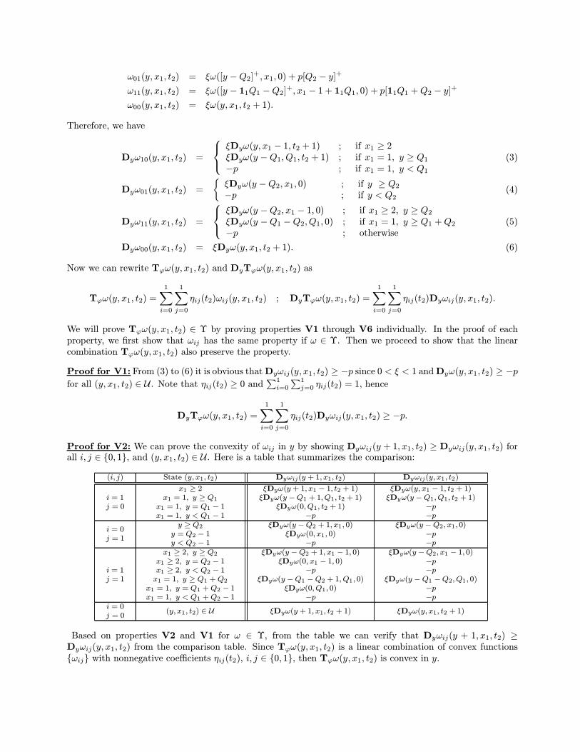
Therefore, we have

Dyω10(y, x1, t2) =

ξDyω(y, x1 − 1, t2 + 1) ; if x1 ≥ 2ξDyω(y −Q1, Q1, t2 + 1) ; if x1 = 1, y ≥ Q1−p ; if x1 = 1, y < Q1

(3)

Dyω01(y, x1, t2) =

½ξDyω(y −Q2, x1, 0) ; if y ≥ Q2−p ; if y < Q2

(4)

Dyω11(y, x1, t2) =

ξDyω(y −Q2, x1 − 1, 0) ; if x1 ≥ 2, y ≥ Q2ξDyω(y −Q1 −Q2, Q1, 0) ; if x1 = 1, y ≥ Q1 +Q2−p ; otherwise

(5)

Dyω00(y, x1, t2) = ξDyω(y, x1, t2 + 1). (6)

Now we can rewrite Tϕω(y, x1, t2) and DyTϕω(y, x1, t2) as

Tϕω(y, x1, t2) =

1Xi=0

1Xj=0

ηij(t2)ωij(y, x1, t2) ; DyTϕω(y, x1, t2) =

1Xi=0

1Xj=0

ηij(t2)Dyωij(y, x1, t2).

We will prove Tϕω(y, x1, t2) ∈ Υ by proving properties V1 through V6 individually. In the proof of eachproperty, we Þrst show that ωij has the same property if ω ∈ Υ. Then we proceed to show that the linearcombination Tϕω(y, x1, t2) also preserve the property.

Proof for V1: From (3) to (6) it is obvious thatDyωij(y, x1, t2) ≥ −p since 0 < ξ < 1 andDyω(y, x1, t2) ≥ −pfor all (y, x1, t2) ∈ U . Note that ηij(t2) ≥ 0 and

P1i=0

P1j=0 ηij(t2) = 1, hence

DyTϕω(y, x1, t2) =

1Xi=0

1Xj=0

ηij(t2)Dyωij(y, x1, t2) ≥ −p.

Proof for V2: We can prove the convexity of ωij in y by showing Dyωij(y + 1, x1, t2) ≥ Dyωij(y, x1, t2) forall i, j ∈ {0, 1}, and (y, x1, t2) ∈ U . Here is a table that summarizes the comparison:

(i, j) State (y, x1, t2) Dyωij(y + 1, x1, t2) Dyωij(y, x1, t2)

i = 1j = 0

x1 ≥ 2x1 = 1, y ≥ Q1

x1 = 1, y = Q1 − 1x1 = 1, y < Q1 − 1

ξDyω(y + 1, x1 − 1, t2 + 1)ξDyω(y −Q1 + 1,Q1, t2 + 1)

ξDyω(0,Q1, t2 + 1)−p

ξDyω(y, x1 − 1, t2 + 1)ξDyω(y −Q1,Q1, t2 + 1)

−p−p

i = 0j = 1

y ≥ Q2y = Q2 − 1y < Q2 − 1

ξDyω(y −Q2 + 1, x1, 0)ξDyω(0, x1, 0)

−p

ξDyω(y −Q2, x1, 0)−p−p

i = 1j = 1

x1 ≥ 2, y ≥ Q2x1 ≥ 2, y = Q2 − 1x1 ≥ 2, y < Q2 − 1x1 = 1, y ≥ Q1 +Q2

x1 = 1, y = Q1 +Q2 − 1x1 = 1, y < Q1 +Q2 − 1

ξDyω(y −Q2 + 1, x1 − 1, 0)ξDyω(0, x1 − 1, 0)

−pξDyω(y −Q1 −Q2 + 1, Q1, 0)

ξDyω(0,Q1, 0)−p

ξDyω(y −Q2, x1 − 1, 0)−p−p

ξDyω(y −Q1 −Q2, Q1, 0)−p−p

i = 0j = 0

(y, x1, t2) ∈ U ξDyω(y + 1, x1, t2 + 1) ξDyω(y, x1, t2 + 1)

Based on properties V2 and V1 for ω ∈ Υ, from the table we can verify that Dyωij(y + 1, x1, t2) ≥Dyωij(y, x1, t2) from the comparison table. Since Tϕω(y, x1, t2) is a linear combination of convex functions{ωij} with nonnegative coefficients ηij(t2), i, j ∈ {0, 1}, then Tϕω(y, x1, t2) is convex in y.

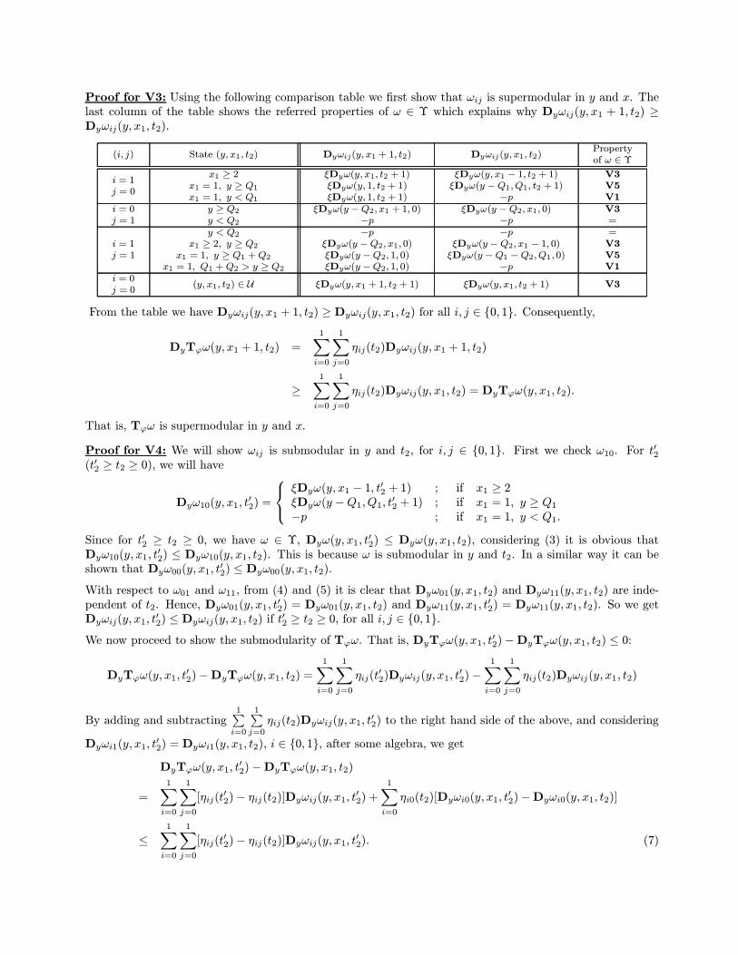
Proof for V3: Using the following comparison table we Þrst show that ωij is supermodular in y and x. Thelast column of the table shows the referred properties of ω ∈ Υ which explains why Dyωij(y, x1 + 1, t2) ≥Dyωij(y, x1, t2).

(i, j) State (y, x1, t2) Dyωij(y, x1 + 1, t2) Dyωij(y, x1, t2)Propertyof ω ∈ Υ

i = 1j = 0

x1 ≥ 2x1 = 1, y ≥ Q1x1 = 1, y < Q1

ξDyω(y, x1, t2 + 1)ξDyω(y, 1, t2 + 1)ξDyω(y, 1, t2 + 1)

ξDyω(y, x1 − 1, t2 + 1)ξDyω(y −Q1,Q1, t2 + 1)

−p

V3V5V1

i = 0j = 1

y ≥ Q2y < Q2

ξDyω(y −Q2, x1 + 1, 0)−p

ξDyω(y −Q2, x1, 0)−p

V3=

i = 1j = 1

y < Q2x1 ≥ 2, y ≥ Q2

x1 = 1, y ≥ Q1 +Q2x1 = 1, Q1 +Q2 > y ≥ Q2

−pξDyω(y −Q2, x1, 0)ξDyω(y −Q2, 1, 0)ξDyω(y −Q2, 1, 0)

−pξDyω(y −Q2, x1 − 1, 0)ξDyω(y −Q1 −Q2,Q1, 0)

−p

=V3V5V1

i = 0j = 0

(y, x1, t2) ∈ U ξDyω(y, x1 + 1, t2 + 1) ξDyω(y, x1, t2 + 1) V3

From the table we have Dyωij(y, x1 + 1, t2) ≥ Dyωij(y, x1, t2) for all i, j ∈ {0, 1}. Consequently,

DyTϕω(y, x1 + 1, t2) =

1Xi=0

1Xj=0

ηij(t2)Dyωij(y, x1 + 1, t2)

≥1Xi=0

1Xj=0

ηij(t2)Dyωij(y, x1, t2) = DyTϕω(y, x1, t2).

That is, Tϕω is supermodular in y and x.

Proof for V4: We will show ωij is submodular in y and t2, for i, j ∈ {0, 1}. First we check ω10. For t02(t02 ≥ t2 ≥ 0), we will have

Dyω10(y, x1, t02) =

ξDyω(y, x1 − 1, t02 + 1) ; if x1 ≥ 2ξDyω(y −Q1, Q1, t02 + 1) ; if x1 = 1, y ≥ Q1−p ; if x1 = 1, y < Q1.

Since for t02 ≥ t2 ≥ 0, we have ω ∈ Υ, Dyω(y, x1, t02) ≤ Dyω(y, x1, t2), considering (3) it is obvious that

Dyω10(y, x1, t02) ≤ Dyω10(y, x1, t2). This is because ω is submodular in y and t2. In a similar way it can be

shown that Dyω00(y, x1, t02) ≤ Dyω00(y, x1, t2).

With respect to ω01 and ω11, from (4) and (5) it is clear that Dyω01(y, x1, t2) and Dyω11(y, x1, t2) are inde-pendent of t2. Hence, Dyω01(y, x1, t

02) = Dyω01(y, x1, t2) and Dyω11(y, x1, t

02) = Dyω11(y, x1, t2). So we get

Dyωij(y, x1, t02) ≤ Dyωij(y, x1, t2) if t

02 ≥ t2 ≥ 0, for all i, j ∈ {0, 1}.

We now proceed to show the submodularity of Tϕω. That is, DyTϕω(y, x1, t02)−DyTϕω(y, x1, t2) ≤ 0:

DyTϕω(y, x1, t02)−DyTϕω(y, x1, t2) =

1Xi=0

1Xj=0

ηij(t02)Dyωij(y, x1, t

02)−

1Xi=0

1Xj=0

ηij(t2)Dyωij(y, x1, t2)

By adding and subtracting1Pi=0

1Pj=0

ηij(t2)Dyωij(y, x1, t02) to the right hand side of the above, and considering

Dyωi1(y, x1, t02) = Dyωi1(y, x1, t2), i ∈ {0, 1}, after some algebra, we getDyTϕω(y, x1, t

02)−DyTϕω(y, x1, t2)

=

1Xi=0

1Xj=0

[ηij(t02)− ηij(t2)]Dyωij(y, x1, t

02) +

1Xi=0

ηi0(t2)[Dyωi0(y, x1, t02)−Dyωi0(y, x1, t2)]

≤1Xi=0

1Xj=0

[ηij(t02)− ηij(t2)]Dyωij(y, x1, t

02). (7)

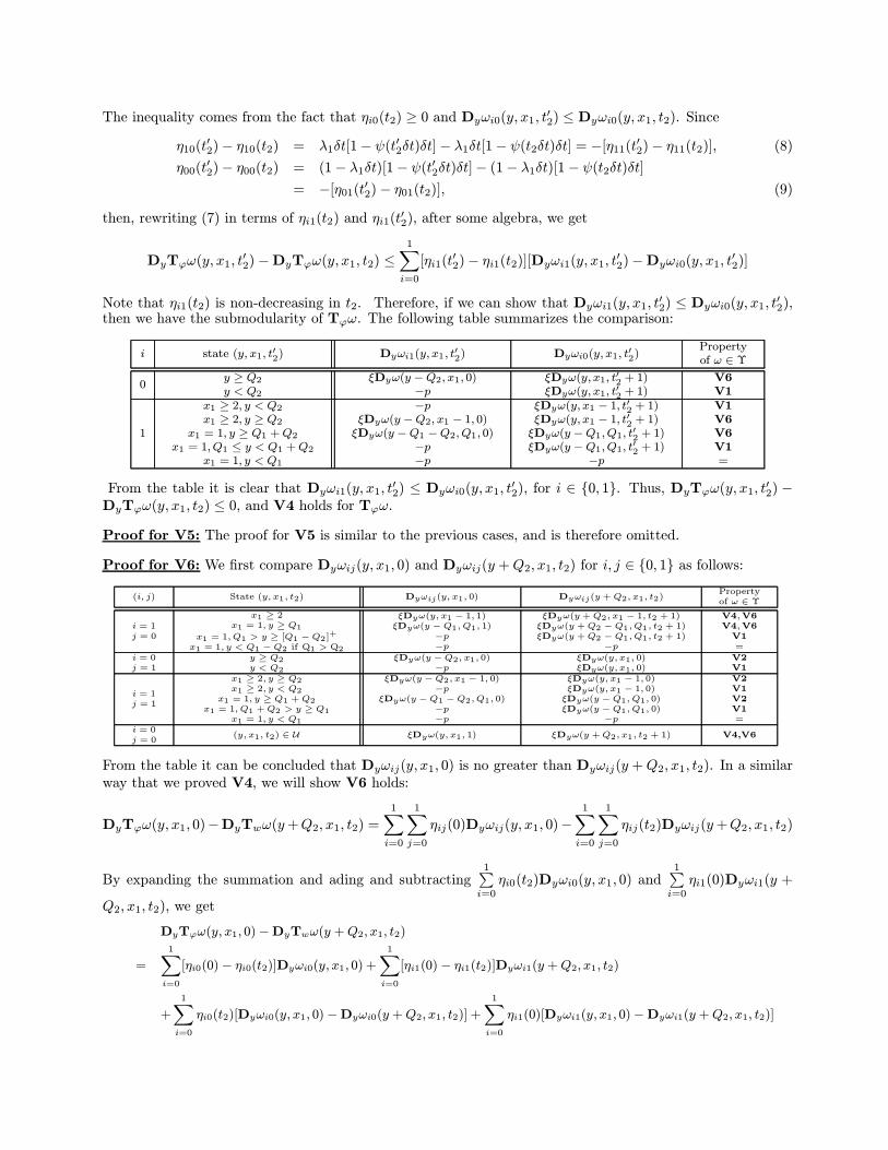
The inequality comes from the fact that ηi0(t2) ≥ 0 and Dyωi0(y, x1, t02) ≤ Dyωi0(y, x1, t2). Since

η10(t02)− η10(t2) = λ1δt[1− ψ(t02δt)δt]− λ1δt[1− ψ(t2δt)δt] = −[η11(t02)− η11(t2)], (8)

η00(t02)− η00(t2) = (1− λ1δt)[1− ψ(t02δt)δt]− (1− λ1δt)[1− ψ(t2δt)δt]

= −[η01(t02)− η01(t2)], (9)

then, rewriting (7) in terms of ηi1(t2) and ηi1(t02), after some algebra, we get

DyTϕω(y, x1, t02)−DyTϕω(y, x1, t2) ≤

1Xi=0

[ηi1(t02)− ηi1(t2)][Dyωi1(y, x1, t

02)−Dyωi0(y, x1, t

02)]

Note that ηi1(t2) is non-decreasing in t2. Therefore, if we can show that Dyωi1(y, x1, t02) ≤ Dyωi0(y, x1, t

02),

then we have the submodularity of Tϕω. The following table summarizes the comparison:

i state (y, x1, t02) Dyωi1(y, x1, t02) Dyωi0(y, x1, t

02)

Propertyof ω ∈ Υ

0y ≥ Q2y < Q2

ξDyω(y −Q2, x1, 0)−p

ξDyω(y, x1, t02 + 1)ξDyω(y, x1, t02 + 1)

V6V1

1

x1 ≥ 2, y < Q2x1 ≥ 2, y ≥ Q2

x1 = 1, y ≥ Q1 +Q2x1 = 1,Q1 ≤ y < Q1 +Q2

x1 = 1, y < Q1

−pξDyω(y −Q2, x1 − 1, 0)ξDyω(y −Q1 −Q2, Q1, 0)

−p−p

ξDyω(y, x1 − 1, t02 + 1)ξDyω(y, x1 − 1, t02 + 1)ξDyω(y −Q1,Q1, t02 + 1)ξDyω(y −Q1,Q1, t02 + 1)−p

V1V6V6V1=

From the table it is clear that Dyωi1(y, x1, t02) ≤ Dyωi0(y, x1, t

02), for i ∈ {0, 1}. Thus, DyTϕω(y, x1, t

02) −

DyTϕω(y, x1, t2) ≤ 0, and V4 holds for Tϕω.Proof for V5: The proof for V5 is similar to the previous cases, and is therefore omitted.

Proof for V6: We Þrst compare Dyωij(y, x1, 0) and Dyωij(y +Q2, x1, t2) for i, j ∈ {0, 1} as follows:(i, j) State (y, x1, t2) Dyωij(y, x1, 0) Dyωij(y +Q2, x1, t2)

Propertyof ω ∈ Υ

i = 1j = 0

x1 ≥ 2x1 = 1, y ≥ Q1

x1 = 1,Q1 > y ≥ [Q1 −Q2]+

x1 = 1, y < Q1 −Q2 if Q1 > Q2

ξDyω(y, x1 − 1, 1)ξDyω(y −Q1, Q1, 1)

−p−p

ξDyω(y +Q2, x1 − 1, t2 + 1)ξDyω(y +Q2 −Q1,Q1, t2 + 1)ξDyω(y +Q2 −Q1,Q1, t2 + 1)

−p

V4,V6V4,V6V1=

i = 0j = 1

y ≥ Q2y < Q2

ξDyω(y −Q2, x1, 0)−p

ξDyω(y, x1, 0)ξDyω(y, x1, 0)

V2V1

i = 1j = 1

x1 ≥ 2, y ≥ Q2x1 ≥ 2, y < Q2

x1 = 1, y ≥ Q1 +Q2x1 = 1, Q1 +Q2 > y ≥ Q1

x1 = 1, y < Q1

ξDyω(y −Q2, x1 − 1, 0)−p

ξDyω(y −Q1 −Q2,Q1, 0)−p−p

ξDyω(y, x1 − 1, 0)ξDyω(y, x1 − 1, 0)ξDyω(y −Q1, Q1, 0)ξDyω(y −Q1, Q1, 0)

−p

V2V1V2V1=

i = 0j = 0

(y, x1, t2) ∈ U ξDyω(y, x1, 1) ξDyω(y +Q2, x1, t2 + 1) V4,V6

From the table it can be concluded that Dyωij(y, x1, 0) is no greater than Dyωij(y +Q2, x1, t2). In a similarway that we proved V4, we will show V6 holds:

DyTϕω(y, x1, 0)−DyTwω(y+Q2, x1, t2) =

1Xi=0

1Xj=0

ηij(0)Dyωij(y, x1, 0)−1Xi=0

1Xj=0

ηij(t2)Dyωij(y+Q2, x1, t2)

By expanding the summation and ading and subtracting1Pi=0

ηi0(t2)Dyωi0(y, x1, 0) and1Pi=0

ηi1(0)Dyωi1(y +

Q2, x1, t2), we get

DyTϕω(y, x1, 0)−DyTwω(y +Q2, x1, t2)

=

1Xi=0

[ηi0(0)− ηi0(t2)]Dyωi0(y, x1, 0) +

1Xi=0

[ηi1(0)− ηi1(t2)]Dyωi1(y +Q2, x1, t2)

+

1Xi=0

ηi0(t2)[Dyωi0(y, x1, 0)−Dyωi0(y +Q2, x1, t2)] +

1Xi=0

ηi1(0)[Dyωi1(y, x1, 0)−Dyωi1(y +Q2, x1, t2)]

≤1Xi=0

[ηi0(0)− ηi0(t2)]Dyωi0(y, x1, 0) +

1Xi=0

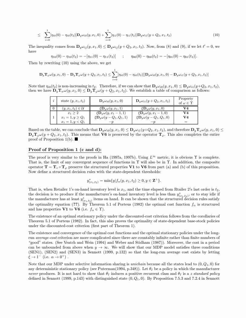
[ηi1(0)− ηi1(t2)]Dyωi1(y +Q2, x1, t2) (10)

The inequality comes from Dyωij(y, x1, 0) ≤ Dyωij(y+Q2, x1, t2). Now, from (8) and (9), if we let t0 = 0, wehave

η10(0)− η10(t2) = −[η11(0)− η11(t2)] ; η00(0)− η00(t2) = −[η01(0)− η01(t2)].Then by rewriting (10) using the above, we get

DyTϕω(y, x1, 0)−DyTϕω(y +Q2, x1, t2) ≤1Xi=0

[ηi0(0)− ηi0(t2)][Dyωi0(y, x1, 0)−Dyωi1(y +Q2, x1, t2)]

Note that ηi0(t2) is non-increasing in t2. Therefore, if we can show thatDyωi0(y, x1, 0) ≤ Dyωi1(y+Q2, x1, t2),then we have DyTwω(y, x1, 0) ≤ DyTϕω(y +Q2, x1, t2). We establish a table of comparison as follows:

i state (y, x1, t2) Dyωi0(y, x1, 0) Dyωi1(y +Q2, x1, t2)Propertyof ω ∈ Υ

0 (y, x1, t2) ∈ U ξDyω(y, x1, 1) ξDyω(y, x1, 0) V4

1x1 ≥ 2

x1 = 1, y ≥ Q1

x1 = 1, y < Q1

ξDyω(y, x1 − 1, 1)ξDyω(y −Q1, Q1, 1)

−p

ξDyω(y, x1 − 1, 0)ξDyω(y −Q1, Q1, 0)

−p

V4V4=

Based on the table, we can conclude thatDyωi0(y, x1, 0) ≤ Dyωi1(y+Q2, x1, t2), and thereforeDyTϕω(y, x1, 0) ≤DyTϕω(y +Q2, x1, t2). This means that V6 is preserved by the operator Tϕ. This also completes the entireproof of Proposition 1(b).

Proof of Proposition 1 (c and d):

The proof is very similar to the proofs in Ha (1997a, 1997b). Using L∞ metric, it is obvious Υ is complete.That is, the limit of any convergent sequence of functions in Υ will also be in Υ. In addition, the compositeoperator T = Tv ◦Tϕ preserve the structured properties V1 to V6 from part (a) and (b) of this proposition.Now deÞne a structured decision rules with the state-dependent thresholds:

y∗(x1,t2) = min{y|fα(y, x1, t2) ≥ 0, y ∈ Z+}.

That is, when Retailer 1�s on-hand inventory level is x1, and the time elapsed from Rtailer 2�s last order is t2,the decision is to produce if the manufacturer�s on-hand inventory level is less than y∗(x1,t2), or to stay idle ifthe manufacturer has at least y∗(x1,t2) items on hand. It can be shown that the structured decision rules satisfythe optimality equation (??). By Theorem 5.1 of Porteus (1982) the optimal cost function fα is structuredand has properties V1 to V6 (i.e. fα ∈ Υ).The existence of an optimal stationary policy under the discounted-cost criterion follows from the corollaries ofTheorem 5.1 of Porteus (1982). In fact, this also proves the optimality of state-dependent base-stock policiesunder the discounted-cost criterion (Þrst part of Theorem 1).

The existence and convergence of the optimal cost functions and the optimal stationary policies under the long-run average-cost criterion are more complicated since there are countably inÞnite rather than Þnite numbers of�good� states. (See Veatch and Wein (1994) and Weber and Stidham (1987)). Moreover, the cost in a periodcan be unbounded from above when y → ∞. We will show that our MDP model satisÞes three conditions(SEN1), (SEN2) and (SEN3) in Sennott (1999, p.132) so that the long-run average cost exists by lettingξ → 1− (i.e. α→ 0+) .

Note that our MDP under selective information sharing is unichain because all the states lead to (0, Q1, 0) forany deterministic stationary policy (see Puterman(1994, p.348)). Let θI be a policy in which the manufacturernever produces. It is not hard to show that θI induces a positive recurrent class and θI is a z standard policydeÞned in Sennott (1999, p.143) with distinguished state (0, Q1, 0). By Proposition 7.5.3 and 7.2.4 in Sennott

(1999), (SEN1) and (SEN2) hold for every state in U . Now we can Þnd the one-step expected cost function(i.e., expected cots during δt) under θI :

CθI (y, x1, t2) = h(y)δt+ p¡η10(t2)[11Q1 − y]+

+η01(t2)[Q2 − y]+ + η11(t2)[11Q1 +Q2 − y]+¢.

It can be shown that 0 ≤ CθI (y, x1, t2) ≤ h(y)δt + (Q1 + Q2)p. As a result, the total discounted-cost underthe optimal policy starting at state (y, x1, t2) has a lower bound and an upper bound:

0 ≤ fα(y, x1, t2) ≤ 1

1− ξ [h(y)δt+ (Q1 +Q2)p].

Now, we let M be the optimal total discounted-cost associated with the distinguished state (0, Q1, 0), then weget

fα(y, x1, t2)− fα(0, Q1, 0) ≥ 0− fα(0, Q1, 0) = −Mfor all (y, x1, t2) ∈ U . Thus, (SEN3) holds and the long-run average cost exists by Theorem 7.2.3 in Sennott(1999). By the same theorem, any limit point of the optimal stationary policies under total discount-costcriterion is average-cost optimal. The limit point can be obtained by appropriately choosing a sequence{ξn}→ 1−.

Proof of Theorem 1

Under discounted-cost criterion, the optimality of state-dependent base-stock policies have been shown in theproof of Proposition 1(c)(d). Because fα and mξ are convex in y (note that mξ = Tϕfα), from V2 and Lemma1 we can conclude that, for any state ( ·, x1, t2), there exists an inventory level y∗(x1,t2) ≥ 0 such that, for ally < y∗(x1,t2), the optimal decision at (y, x1, t2) is production. On the other hand, for all y ≥ y∗(x1,t2), the optimaldecision at (y, x1, t2) is idleness. In addition, by Theorem 7.2.3 in Sennott (1999) state-dependent base-stockpolicies are also average-cost optimal as it is the limit point of optimal policies under the discounted-costcriterion.

Proof of Theorem 2

The proof of Theorem 2 also comes directly from the convexity, supermodularity and submodularity ofmξ(y, x1, t2) (i.e., properties V2, V3 and V4) and Lemma 1. For example, if the base stock level at (y, x1, t2)is y∗(x1,t2), then from V2, V4 and Lemma 1, we get

Dymξ(y, x1, t02) < 0 ; for all y < y∗(x1,t2) and t02 ≥ t2.

This implies that, when t02 ≤ t2, the optimal base-stock level y∗(x1,t02)

at state ( ·, x1, t02) is not lower thany∗(x1,t2). In other words, the optimal base-stock level is non-decreasing in t2. A similar approach can be usedto show that the optimal base-stock levels are non-increasing in x1. The same properties hold in average-costoptimal policies by letting α→ 0+, as shown in the proofs of Proposition 1(c and d) and Theorem 1.

Proof of Theorem 3

The proof of Theorem 3 also comes directly from the properties of function mξ(y, x1, t2) (i.e., properties V2,V5, and V6) and Lemma 1. The same properties hold in average-cost optimal policies by letting α→ 0+, asshown in the proofs of Proposition 1(c and d) and Theorem 1.

ON-LINE APPENDIX B

Details of the Numerical Study

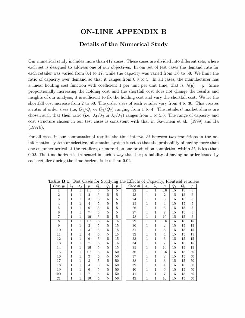
Our numerical study includes more than 417 cases. These cases are divided into different sets, where

each set is designed to address one of our objectives. In our set of test cases the demand rate for

each retailer was varied from 0.4 to 17, while the capacity was varied from 1.6 to 50. We limit the

ratio of capacity over demand so that it ranges from 0.8 to 5. In all cases, the manufacturer has

a linear holding cost function with coefficient 1 per unit per unit time, that is, h(y) = y. Since

proportionally increasing the holding cost and the shortfall cost does not change the results and

insights of our analysis, it is sufficient to Þx the holding cost and vary the shortfall cost. We let the

shortfall cost increase from 2 to 50. The order sizes of each retailer vary from 4 to 30. This creates

a ratio of order sizes (i.e, Q1/Q2 or Q2/Q2) ranging from 1 to 4. The retailers� market shares are

chosen such that their ratio (i.e., λ1/λ2 or λ2/λ2) ranges from 1 to 5.6. The range of capacity and

cost structure chosen in our test cases is consistent with that in Gavirneni et al. (1999) and Ha

(1997b).

For all cases in our computational results, the time interval δt between two transitions in the no-

information system or selective-information system is set so that the probability of having more than

one customer arrival at the retailers, or more than one production completion within δt, is less than

0.02. The time horizon is truncated in such a way that the probability of having no order issued by

each retailer during the time horizon is less than 0.02.

Table B.1. Test Cases for Studying the Effects of Capacity, Identical retailersCase # λ1 λ2 µ Q1 Q1 p Case # λ1 λ2 µ Q1 Q1 p1 1 1 1.6 5 5 5 22 1 1 1.6 15 15 52 1 1 2 5 5 5 23 1 1 2 15 15 53 1 1 3 5 5 5 24 1 1 3 15 15 54 1 1 4 5 5 5 25 1 1 4 15 15 55 1 1 6 5 5 5 26 1 1 6 15 15 56 1 1 7 5 5 5 27 1 1 7 15 15 57 1 1 10 5 5 5 28 1 1 10 15 15 58 1 1 1.6 5 5 15 29 1 1 1.6 15 15 159 1 1 2 5 5 15 30 1 1 2 15 15 1510 1 1 3 5 5 15 31 1 1 3 15 15 1511 1 1 4 5 5 15 32 1 1 4 15 15 1512 1 1 6 5 5 15 33 1 1 6 15 15 1513 1 1 7 5 5 15 34 1 1 7 15 15 1514 1 1 10 5 5 15 35 1 1 10 15 15 1515 1 1 1.6 5 5 50 36 1 1 1.6 15 15 5016 1 1 2 5 5 50 37 1 1 2 15 15 5017 1 1 3 5 5 50 38 1 1 3 15 15 5018 1 1 4 5 5 50 39 1 1 4 15 15 5019 1 1 6 5 5 50 40 1 1 6 15 15 5020 1 1 7 5 5 50 41 1 1 7 15 15 5021 1 1 10 5 5 50 42 1 1 10 15 15 50

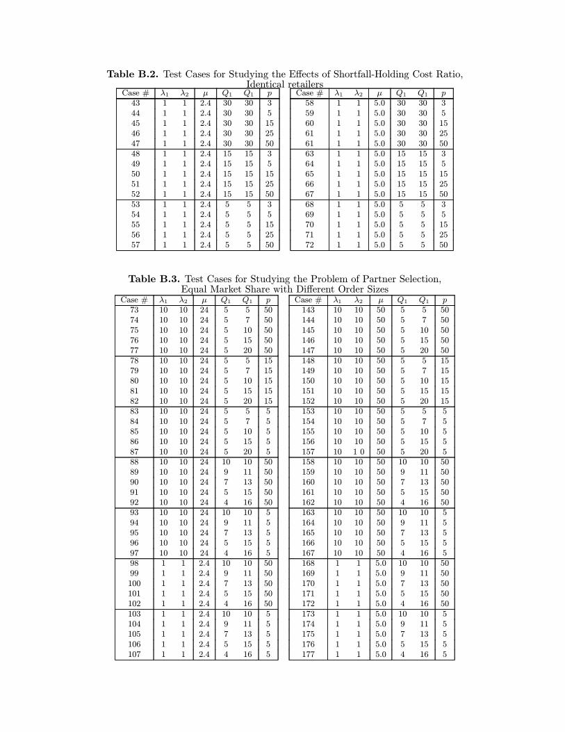
Table B.2. Test Cases for Studying the Effects of Shortfall-Holding Cost Ratio,Identical retailers

Case # λ1 λ2 µ Q1 Q1 p Case # λ1 λ2 µ Q1 Q1 p43 1 1 2.4 30 30 3 58 1 1 5.0 30 30 344 1 1 2.4 30 30 5 59 1 1 5.0 30 30 545 1 1 2.4 30 30 15 60 1 1 5.0 30 30 1546 1 1 2.4 30 30 25 61 1 1 5.0 30 30 2547 1 1 2.4 30 30 50 61 1 1 5.0 30 30 5048 1 1 2.4 15 15 3 63 1 1 5.0 15 15 349 1 1 2.4 15 15 5 64 1 1 5.0 15 15 550 1 1 2.4 15 15 15 65 1 1 5.0 15 15 1551 1 1 2.4 15 15 25 66 1 1 5.0 15 15 2552 1 1 2.4 15 15 50 67 1 1 5.0 15 15 5053 1 1 2.4 5 5 3 68 1 1 5.0 5 5 354 1 1 2.4 5 5 5 69 1 1 5.0 5 5 555 1 1 2.4 5 5 15 70 1 1 5.0 5 5 1556 1 1 2.4 5 5 25 71 1 1 5.0 5 5 2557 1 1 2.4 5 5 50 72 1 1 5.0 5 5 50

Table B.3. Test Cases for Studying the Problem of Partner Selection,Equal Market Share with Different Order Sizes

Case # λ1 λ2 µ Q1 Q1 p Case # λ1 λ2 µ Q1 Q1 p73 10 10 24 5 5 50 143 10 10 50 5 5 5074 10 10 24 5 7 50 144 10 10 50 5 7 5075 10 10 24 5 10 50 145 10 10 50 5 10 5076 10 10 24 5 15 50 146 10 10 50 5 15 5077 10 10 24 5 20 50 147 10 10 50 5 20 5078 10 10 24 5 5 15 148 10 10 50 5 5 1579 10 10 24 5 7 15 149 10 10 50 5 7 1580 10 10 24 5 10 15 150 10 10 50 5 10 1581 10 10 24 5 15 15 151 10 10 50 5 15 1582 10 10 24 5 20 15 152 10 10 50 5 20 1583 10 10 24 5 5 5 153 10 10 50 5 5 584 10 10 24 5 7 5 154 10 10 50 5 7 585 10 10 24 5 10 5 155 10 10 50 5 10 586 10 10 24 5 15 5 156 10 10 50 5 15 587 10 10 24 5 20 5 157 10 1 0 50 5 20 588 10 10 24 10 10 50 158 10 10 50 10 10 5089 10 10 24 9 11 50 159 10 10 50 9 11 5090 10 10 24 7 13 50 160 10 10 50 7 13 5091 10 10 24 5 15 50 161 10 10 50 5 15 5092 10 10 24 4 16 50 162 10 10 50 4 16 5093 10 10 24 10 10 5 163 10 10 50 10 10 594 10 10 24 9 11 5 164 10 10 50 9 11 595 10 10 24 7 13 5 165 10 10 50 7 13 596 10 10 24 5 15 5 166 10 10 50 5 15 597 10 10 24 4 16 5 167 10 10 50 4 16 598 1 1 2.4 10 10 50 168 1 1 5.0 10 10 5099 1 1 2.4 9 11 50 169 1 1 5.0 9 11 50100 1 1 2.4 7 13 50 170 1 1 5.0 7 13 50101 1 1 2.4 5 15 50 171 1 1 5.0 5 15 50102 1 1 2.4 4 16 50 172 1 1 5.0 4 16 50103 1 1 2.4 10 10 5 173 1 1 5.0 10 10 5104 1 1 2.4 9 11 5 174 1 1 5.0 9 11 5105 1 1 2.4 7 13 5 175 1 1 5.0 7 13 5106 1 1 2.4 5 15 5 176 1 1 5.0 5 15 5107 1 1 2.4 4 16 5 177 1 1 5.0 4 16 5

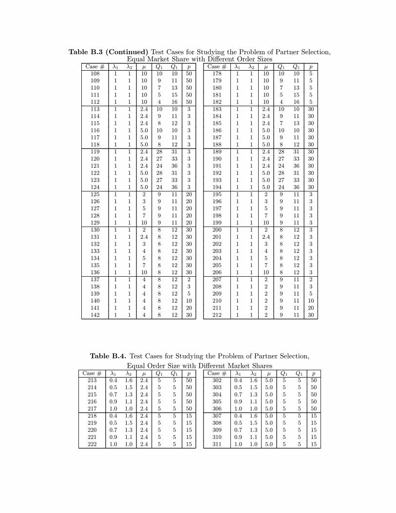
Table B.3 (Continued) Test Cases for Studying the Problem of Partner Selection,Equal Market Share with Different Order Sizes

Case # λ1 λ2 µ Q1 Q1 p Case # λ1 λ2 µ Q1 Q1 p108 1 1 10 10 10 50 178 1 1 10 10 10 5109 1 1 10 9 11 50 179 1 1 10 9 11 5110 1 1 10 7 13 50 180 1 1 10 7 13 5111 1 1 10 5 15 50 181 1 1 10 5 15 5112 1 1 10 4 16 50 182 1 1 10 4 16 5113 1 1 2.4 10 10 3 183 1 1 2.4 10 10 30114 1 1 2.4 9 11 3 184 1 1 2.4 9 11 30115 1 1 2.4 8 12 3 185 1 1 2.4 7 13 30116 1 1 5.0 10 10 3 186 1 1 5.0 10 10 30117 1 1 5.0 9 11 3 187 1 1 5.0 9 11 30118 1 1 5.0 8 12 3 188 1 1 5.0 8 12 30119 1 1 2.4 28 31 3 189 1 1 2.4 28 31 30120 1 1 2.4 27 33 3 190 1 1 2.4 27 33 30121 1 1 2.4 24 36 3 191 1 1 2.4 24 36 30122 1 1 5.0 28 31 3 192 1 1 5.0 28 31 30123 1 1 5.0 27 33 3 193 1 1 5.0 27 33 30124 1 1 5.0 24 36 3 194 1 1 5.0 24 36 30125 1 1 2 9 11 20 195 1 1 2 9 11 3126 1 1 3 9 11 20 196 1 1 3 9 11 3127 1 1 5 9 11 20 197 1 1 5 9 11 3128 1 1 7 9 11 20 198 1 1 7 9 11 3129 1 1 10 9 11 20 199 1 1 10 9 11 3130 1 1 2 8 12 30 200 1 1 2 8 12 3131 1 1 2.4 8 12 30 201 1 1 2.4 8 12 3132 1 1 3 8 12 30 202 1 1 3 8 12 3133 1 1 4 8 12 30 203 1 1 4 8 12 3134 1 1 5 8 12 30 204 1 1 5 8 12 3135 1 1 7 8 12 30 205 1 1 7 8 12 3136 1 1 10 8 12 30 206 1 1 10 8 12 3137 1 1 4 8 12 2 207 1 1 2 9 11 2138 1 1 4 8 12 3 208 1 1 2 9 11 3139 1 1 4 8 12 5 209 1 1 2 9 11 5140 1 1 4 8 12 10 210 1 1 2 9 11 10141 1 1 4 8 12 20 211 1 1 2 9 11 20142 1 1 4 8 12 30 212 1 1 2 9 11 30

Table B.4. Test Cases for Studying the Problem of Partner Selection,

Equal Order Size with Different Market SharesCase # λ1 λ2 µ Q1 Q1 p Case # λ1 λ2 µ Q1 Q1 p213 0.4 1.6 2.4 5 5 50 302 0.4 1.6 5.0 5 5 50214 0.5 1.5 2.4 5 5 50 303 0.5 1.5 5.0 5 5 50215 0.7 1.3 2.4 5 5 50 304 0.7 1.3 5.0 5 5 50216 0.9 1.1 2.4 5 5 50 305 0.9 1.1 5.0 5 5 50217 1.0 1.0 2.4 5 5 50 306 1.0 1.0 5.0 5 5 50218 0.4 1.6 2.4 5 5 15 307 0.4 1.6 5.0 5 5 15219 0.5 1.5 2.4 5 5 15 308 0.5 1.5 5.0 5 5 15220 0.7 1.3 2.4 5 5 15 309 0.7 1.3 5.0 5 5 15221 0.9 1.1 2.4 5 5 15 310 0.9 1.1 5.0 5 5 15222 1.0 1.0 2.4 5 5 15 311 1.0 1.0 5.0 5 5 15

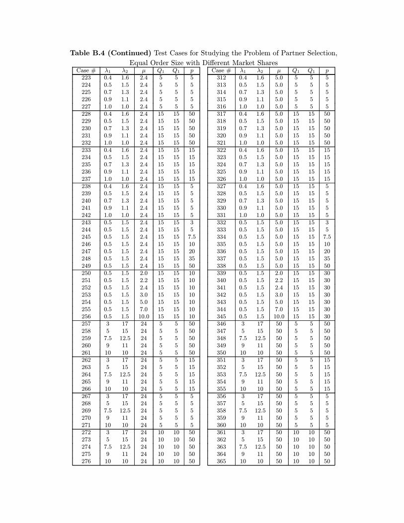
Table B.4 (Continued) Test Cases for Studying the Problem of Partner Selection,

Equal Order Size with Different Market SharesCase # λ1 λ2 µ Q1 Q1 p Case # λ1 λ2 µ Q1 Q1 p223 0.4 1.6 2.4 5 5 5 312 0.4 1.6 5.0 5 5 5224 0.5 1.5 2.4 5 5 5 313 0.5 1.5 5.0 5 5 5225 0.7 1.3 2.4 5 5 5 314 0.7 1.3 5.0 5 5 5226 0.9 1.1 2.4 5 5 5 315 0.9 1.1 5.0 5 5 5227 1.0 1.0 2.4 5 5 5 316 1.0 1.0 5.0 5 5 5228 0.4 1.6 2.4 15 15 50 317 0.4 1.6 5.0 15 15 50229 0.5 1.5 2.4 15 15 50 318 0.5 1.5 5.0 15 15 50230 0.7 1.3 2.4 15 15 50 319 0.7 1.3 5.0 15 15 50231 0.9 1.1 2.4 15 15 50 320 0.9 1.1 5.0 15 15 50232 1.0 1.0 2.4 15 15 50 321 1.0 1.0 5.0 15 15 50233 0.4 1.6 2.4 15 15 15 322 0.4 1.6 5.0 15 15 15234 0.5 1.5 2.4 15 15 15 323 0.5 1.5 5.0 15 15 15235 0.7 1.3 2.4 15 15 15 324 0.7 1.3 5.0 15 15 15236 0.9 1.1 2.4 15 15 15 325 0.9 1.1 5.0 15 15 15237 1.0 1.0 2.4 15 15 15 326 1.0 1.0 5.0 15 15 15238 0.4 1.6 2.4 15 15 5 327 0.4 1.6 5.0 15 15 5239 0.5 1.5 2.4 15 15 5 328 0.5 1.5 5.0 15 15 5240 0.7 1.3 2.4 15 15 5 329 0.7 1.3 5.0 15 15 5241 0.9 1.1 2.4 15 15 5 330 0.9 1.1 5.0 15 15 5242 1.0 1.0 2.4 15 15 5 331 1.0 1.0 5.0 15 15 5243 0.5 1.5 2.4 15 15 3 332 0.5 1.5 5.0 15 15 3244 0.5 1.5 2.4 15 15 5 333 0.5 1.5 5.0 15 15 5245 0.5 1.5 2.4 15 15 7.5 334 0.5 1.5 5.0 15 15 7.5246 0.5 1.5 2.4 15 15 10 335 0.5 1.5 5.0 15 15 10247 0.5 1.5 2.4 15 15 20 336 0.5 1.5 5.0 15 15 20248 0.5 1.5 2.4 15 15 35 337 0.5 1.5 5.0 15 15 35249 0.5 1.5 2.4 15 15 50 338 0.5 1.5 5.0 15 15 50250 0.5 1.5 2.0 15 15 10 339 0.5 1.5 2.0 15 15 30251 0.5 1.5 2.2 15 15 10 340 0.5 1.5 2.2 15 15 30252 0.5 1.5 2.4 15 15 10 341 0.5 1.5 2.4 15 15 30253 0.5 1.5 3.0 15 15 10 342 0.5 1.5 3.0 15 15 30254 0.5 1.5 5.0 15 15 10 343 0.5 1.5 5.0 15 15 30255 0.5 1.5 7.0 15 15 10 344 0.5 1.5 7.0 15 15 30256 0.5 1.5 10.0 15 15 10 345 0.5 1.5 10.0 15 15 30257 3 17 24 5 5 50 346 3 17 50 5 5 50258 5 15 24 5 5 50 347 5 15 50 5 5 50259 7.5 12.5 24 5 5 50 348 7.5 12.5 50 5 5 50260 9 11 24 5 5 50 349 9 11 50 5 5 50261 10 10 24 5 5 50 350 10 10 50 5 5 50262 3 17 24 5 5 15 351 3 17 50 5 5 15263 5 15 24 5 5 15 352 5 15 50 5 5 15264 7.5 12.5 24 5 5 15 353 7.5 12.5 50 5 5 15265 9 11 24 5 5 15 354 9 11 50 5 5 15266 10 10 24 5 5 15 355 10 10 50 5 5 15267 3 17 24 5 5 5 356 3 17 50 5 5 5268 5 15 24 5 5 5 357 5 15 50 5 5 5269 7.5 12.5 24 5 5 5 358 7.5 12.5 50 5 5 5270 9 11 24 5 5 5 359 9 11 50 5 5 5271 10 10 24 5 5 5 360 10 10 50 5 5 5272 3 17 24 10 10 50 361 3 17 50 10 10 50273 5 15 24 10 10 50 362 5 15 50 10 10 50274 7.5 12.5 24 10 10 50 363 7.5 12.5 50 10 10 50275 9 11 24 10 10 50 364 9 11 50 10 10 50276 10 10 24 10 10 50 365 10 10 50 10 10 50

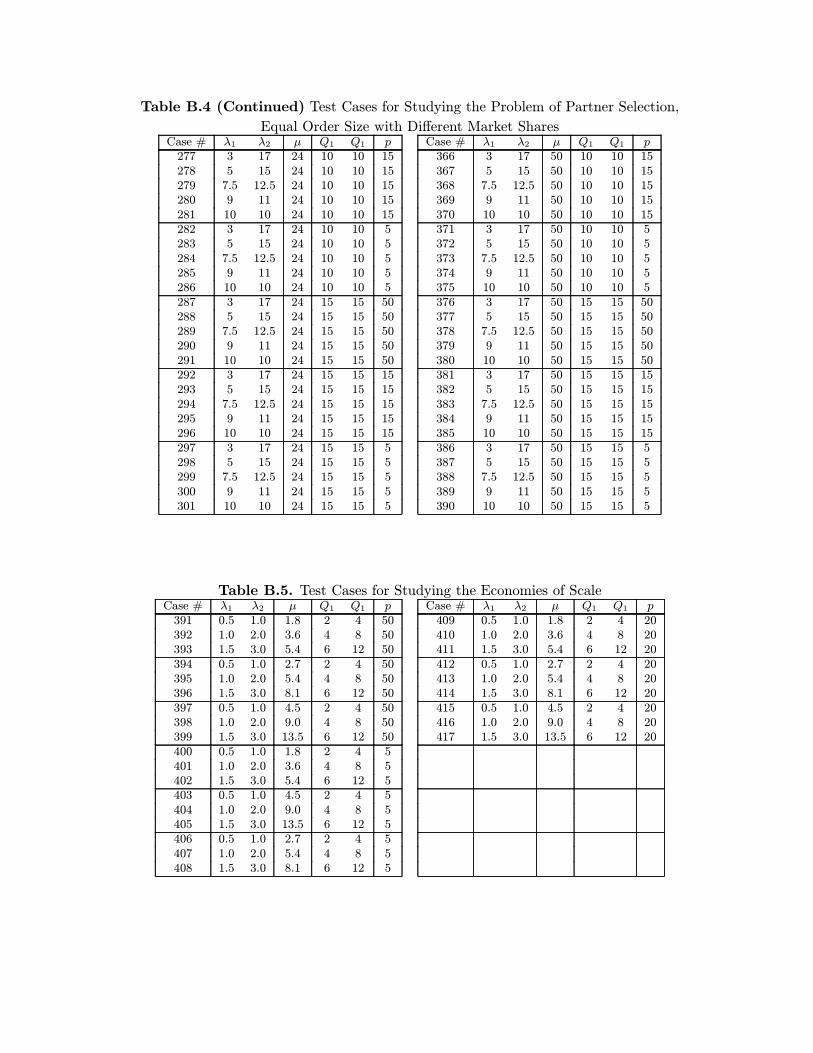
Table B.4 (Continued) Test Cases for Studying the Problem of Partner Selection,

Equal Order Size with Different Market SharesCase # λ1 λ2 µ Q1 Q1 p Case # λ1 λ2 µ Q1 Q1 p277 3 17 24 10 10 15 366 3 17 50 10 10 15278 5 15 24 10 10 15 367 5 15 50 10 10 15279 7.5 12.5 24 10 10 15 368 7.5 12.5 50 10 10 15280 9 11 24 10 10 15 369 9 11 50 10 10 15281 10 10 24 10 10 15 370 10 10 50 10 10 15282 3 17 24 10 10 5 371 3 17 50 10 10 5283 5 15 24 10 10 5 372 5 15 50 10 10 5284 7.5 12.5 24 10 10 5 373 7.5 12.5 50 10 10 5285 9 11 24 10 10 5 374 9 11 50 10 10 5286 10 10 24 10 10 5 375 10 10 50 10 10 5287 3 17 24 15 15 50 376 3 17 50 15 15 50288 5 15 24 15 15 50 377 5 15 50 15 15 50289 7.5 12.5 24 15 15 50 378 7.5 12.5 50 15 15 50290 9 11 24 15 15 50 379 9 11 50 15 15 50291 10 10 24 15 15 50 380 10 10 50 15 15 50292 3 17 24 15 15 15 381 3 17 50 15 15 15293 5 15 24 15 15 15 382 5 15 50 15 15 15294 7.5 12.5 24 15 15 15 383 7.5 12.5 50 15 15 15295 9 11 24 15 15 15 384 9 11 50 15 15 15296 10 10 24 15 15 15 385 10 10 50 15 15 15297 3 17 24 15 15 5 386 3 17 50 15 15 5298 5 15 24 15 15 5 387 5 15 50 15 15 5299 7.5 12.5 24 15 15 5 388 7.5 12.5 50 15 15 5300 9 11 24 15 15 5 389 9 11 50 15 15 5301 10 10 24 15 15 5 390 10 10 50 15 15 5

Table B.5. Test Cases for Studying the Economies of ScaleCase # λ1 λ2 µ Q1 Q1 p Case # λ1 λ2 µ Q1 Q1 p391 0.5 1.0 1.8 2 4 50 409 0.5 1.0 1.8 2 4 20392 1.0 2.0 3.6 4 8 50 410 1.0 2.0 3.6 4 8 20393 1.5 3.0 5.4 6 12 50 411 1.5 3.0 5.4 6 12 20394 0.5 1.0 2.7 2 4 50 412 0.5 1.0 2.7 2 4 20395 1.0 2.0 5.4 4 8 50 413 1.0 2.0 5.4 4 8 20396 1.5 3.0 8.1 6 12 50 414 1.5 3.0 8.1 6 12 20397 0.5 1.0 4.5 2 4 50 415 0.5 1.0 4.5 2 4 20398 1.0 2.0 9.0 4 8 50 416 1.0 2.0 9.0 4 8 20399 1.5 3.0 13.5 6 12 50 417 1.5 3.0 13.5 6 12 20400 0.5 1.0 1.8 2 4 5401 1.0 2.0 3.6 4 8 5402 1.5 3.0 5.4 6 12 5403 0.5 1.0 4.5 2 4 5404 1.0 2.0 9.0 4 8 5405 1.5 3.0 13.5 6 12 5406 0.5 1.0 2.7 2 4 5407 1.0 2.0 5.4 4 8 5408 1.5 3.0 8.1 6 12 5