Homework set 2 1 Hartree product - Purdue Universitywang838/notes/HW/chem_HW.pdf · Homework set 2...
70
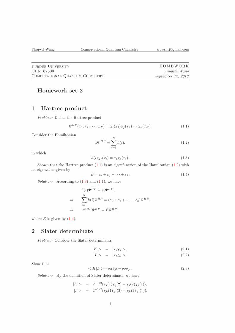
Yingwei Wang Computational Quantum Chemistry [email protected] Purdue University CHM 67300 Computational Quantum Chemistry HOMEWORK Yingwei Wang September 12, 2013 Homework set 2 1 Hartree product Problem: Define the Hartree product Ψ HP (x 1 ,x 2 , ··· ,x N )= χ i (x 1 )χ j (x 2 ) ··· χ k (x N ). (1.1) Consider the Hamiltonian H HP = N i=1 h(i), (1.2) in which h(i)χ j (x i )= ε j χ j (x i ). (1.3) Shown that the Hartree product (1.1) is an eigenfunction of the Hamiltonian (1.2) with an eigenvalue given by E = ε i + ε j + ··· + ε k . (1.4) Solution: According to (1.3) and (1.1), we have h(i)Ψ HP = ε i Ψ HP , ⇒ N i=1 h(i)Ψ HP =(ε i + ε j + ··· + ε k )Ψ HP , ⇒ H HP Ψ HP = EΨ HP , where E is given by (1.4). 2 Slater determinate Problem: Consider the Slater determinants |K> = |χ i χ j >, (2.1) |L> = |χ k χ l >. (2.2) Show that <K|L>= δ ik δ jl − δ il δ jk . (2.3) Solution: By the definition of Slater determinate, we have |K> = 2 -1/2 (χ i (1)χ j (2) − χ i (2)χ j (1)), |L> = 2 -1/2 (χ k (1)χ l (2) − χ k (2)χ l (1)). 1
Transcript of Homework set 2 1 Hartree product - Purdue Universitywang838/notes/HW/chem_HW.pdf · Homework set 2...
Yingwei Wang Computational Quantum Chemistry [email protected]
Purdue University
CHM 67300
Computational Quantum Chemistry
HOMEWORK
Yingwei Wang
September 12, 2013
Homework set 2
1 Hartree product
Problem: Define the Hartree product
ΨHP (x1, x2, · · · , xN ) = χi(x1)χj(x2) · · ·χk(xN ). (1.1)
Consider the Hamiltonian
HHP =
N∑
i=1
h(i), (1.2)
in whichh(i)χj(xi) = εjχj(xi). (1.3)
Shown that the Hartree product (1.1) is an eigenfunction of the Hamiltonian (1.2) withan eigenvalue given by
E = εi + εj + · · ·+ εk. (1.4)
Solution: According to (1.3) and (1.1), we have
h(i)ΨHP = εiΨHP ,
⇒
N∑
i=1
h(i)ΨHP = (εi + εj + · · ·+ εk)ΨHP ,
⇒ HHPΨHP = EΨHP ,
where E is given by (1.4).
2 Slater determinate
Problem: Consider the Slater determinants
|K > = |χiχj >, (2.1)
|L > = |χkχl > . (2.2)
Show that< K|L >= δikδjl − δilδjk. (2.3)
Solution: By the definition of Slater determinate, we have
|K > = 2−1/2(χi(1)χj(2)− χi(2)χj(1)),
|L > = 2−1/2(χk(1)χl(2)− χk(2)χl(1)).
1
Yingwei Wang Computational Quantum Chemistry [email protected]
It follows that
< K|L > = 1/2 [< χi(1)χk(1) >< χj(2)χl(2) > + < χi(2)χk(2) >< χj(1)χl(1) >
− < χi(1)χl(1) >< χj(2)χk(2) > − < χj(1)χk(1) >< χi(2)χl(2) >] ,
= 1/2 [δikδjl + δjlδik − δilδjk − δjkδil] ,
= δikδjl − δilδjk.
Now we verify the (2.3).
3 Self-consistent procedure
Nonlinear Hartree-Fock equations
F (C)C = SCE (3.1)
can be solved by a self-consistent procedure, as follows
1. An initial guess orbitals (matrix C0) are generated;
2. Fock operator is calculated for this set of orbitals (F 0 = F (C0));
3. Fock operator is diagonalized, F 0C1 = SC1E1, and new orbitals C1 replace the orbitalsC0 from previous step;
4. Steps 2-3 are repeated until the difference between orbitals from step n and step n+1is below certain (user-specified) threshold.
Problem: As an example of a non-linear problem, consider the equation
5x2 − 3x− 2 = 0. (3.2)
We can try to find it solution (x = −2/5, 1) by a self-consistent procedure.We can rewrite the equation (3.2) as
x ∗A(x) = 2, A(x) := 5x− 3, (3.3)
where A(x) is a nonlinear coefficient, an analogue of the Fock operator.Solution: The iteration scheme associated with (3.3) is shown in Algorithm 1.
Algorithm 1 Self consistent procedure with (3.3)
1: Initial guess x0.2: for k = 0, 1, 2, · · · do3: Solve xk+1 from the equation
xk+1 =2
5xk − 3. (3.4)
4: Compute the ∆x = xk+1 − xk. If |∆x| < ǫ, then stop.5: end for
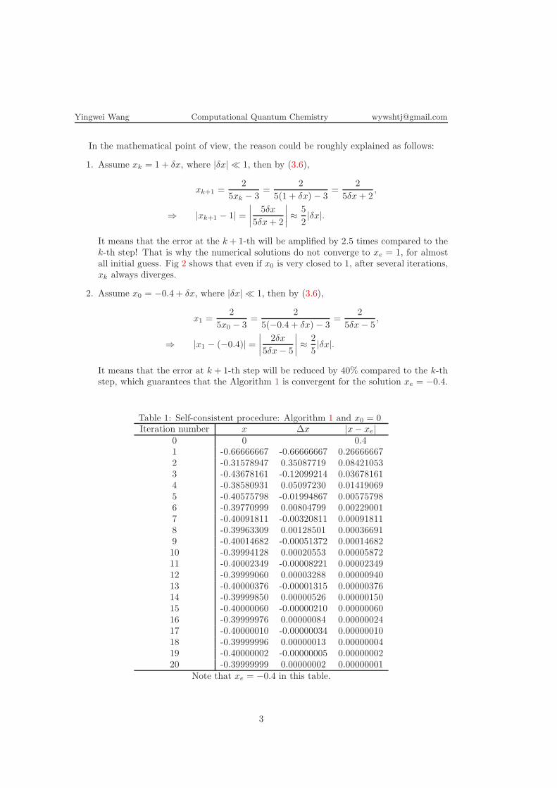
The numerical results for Algorithm 1 with x0 = 0 is shown in Table 1 and Fig.1.Besides, for other initial guess x0, it is highly possible that the numerical solution obtainedby Algorithm 1 converges to x = −0.4 instead of x = 1.
2
Yingwei Wang Computational Quantum Chemistry [email protected]
In the mathematical point of view, the reason could be roughly explained as follows:
1. Assume xk = 1 + δx, where |δx| ≪ 1, then by (3.6),
xk+1 =2
5xk − 3=
2
5(1 + δx) − 3=
2
5δx+ 2,
⇒ |xk+1 − 1| =
∣
∣
∣
∣
5δx
5δx+ 2
∣
∣
∣
∣
≈5
2|δx|.
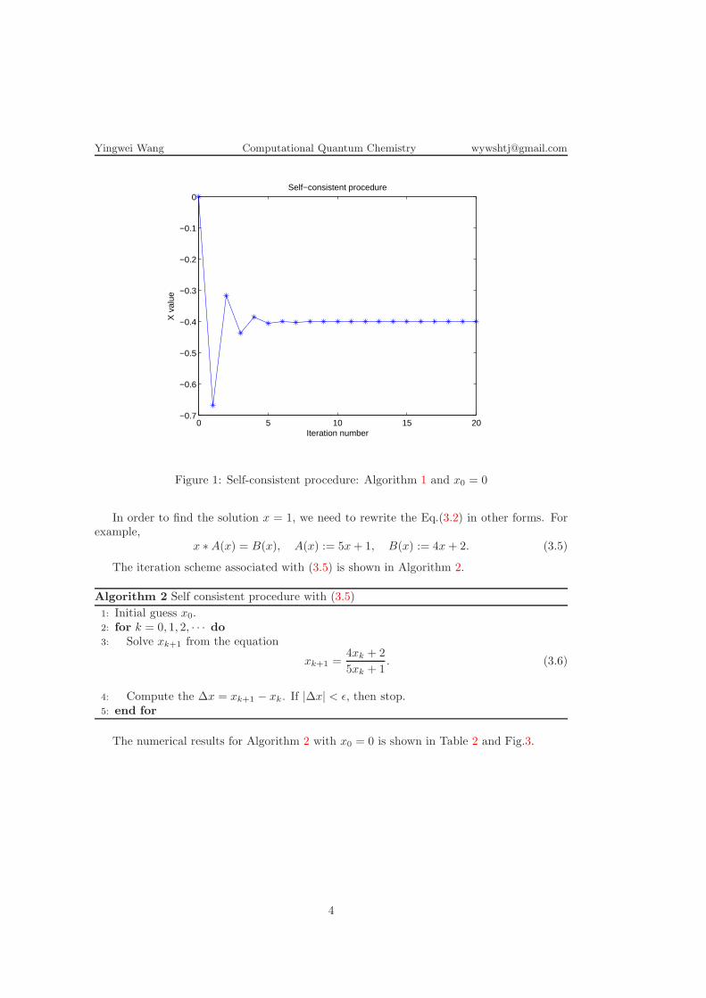
It means that the error at the k+ 1-th will be amplified by 2.5 times compared to thek-th step! That is why the numerical solutions do not converge to xe = 1, for almostall initial guess. Fig 2 shows that even if x0 is very closed to 1, after several iterations,xk always diverges.
2. Assume x0 = −0.4 + δx, where |δx| ≪ 1, then by (3.6),
x1 =2
5x0 − 3=
2
5(−0.4 + δx) − 3=
2
5δx− 5,
⇒ |x1 − (−0.4)| =
∣
∣
∣
∣
2δx
5δx− 5
∣
∣
∣
∣
≈2
5|δx|.
It means that the error at k + 1-th step will be reduced by 40% compared to the k-thstep, which guarantees that the Algorithm 1 is convergent for the solution xe = −0.4.
Table 1: Self-consistent procedure: Algorithm 1 and x0 = 0Iteration number x ∆x |x− xe|
0 0 0.41 -0.66666667 -0.66666667 0.266666672 -0.31578947 0.35087719 0.084210533 -0.43678161 -0.12099214 0.036781614 -0.38580931 0.05097230 0.014190695 -0.40575798 -0.01994867 0.005757986 -0.39770999 0.00804799 0.002290017 -0.40091811 -0.00320811 0.000918118 -0.39963309 0.00128501 0.000366919 -0.40014682 -0.00051372 0.0001468210 -0.39994128 0.00020553 0.0000587211 -0.40002349 -0.00008221 0.0000234912 -0.39999060 0.00003288 0.0000094013 -0.40000376 -0.00001315 0.0000037614 -0.39999850 0.00000526 0.0000015015 -0.40000060 -0.00000210 0.0000006016 -0.39999976 0.00000084 0.0000002417 -0.40000010 -0.00000034 0.0000001018 -0.39999996 0.00000013 0.0000000419 -0.40000002 -0.00000005 0.0000000220 -0.39999999 0.00000002 0.00000001
Note that xe = −0.4 in this table.
3
Yingwei Wang Computational Quantum Chemistry [email protected]
0 5 10 15 20−0.7
−0.6
−0.5
−0.4
−0.3
−0.2
−0.1
0Self−consistent procedure
Iteration number
X v
alue
Figure 1: Self-consistent procedure: Algorithm 1 and x0 = 0
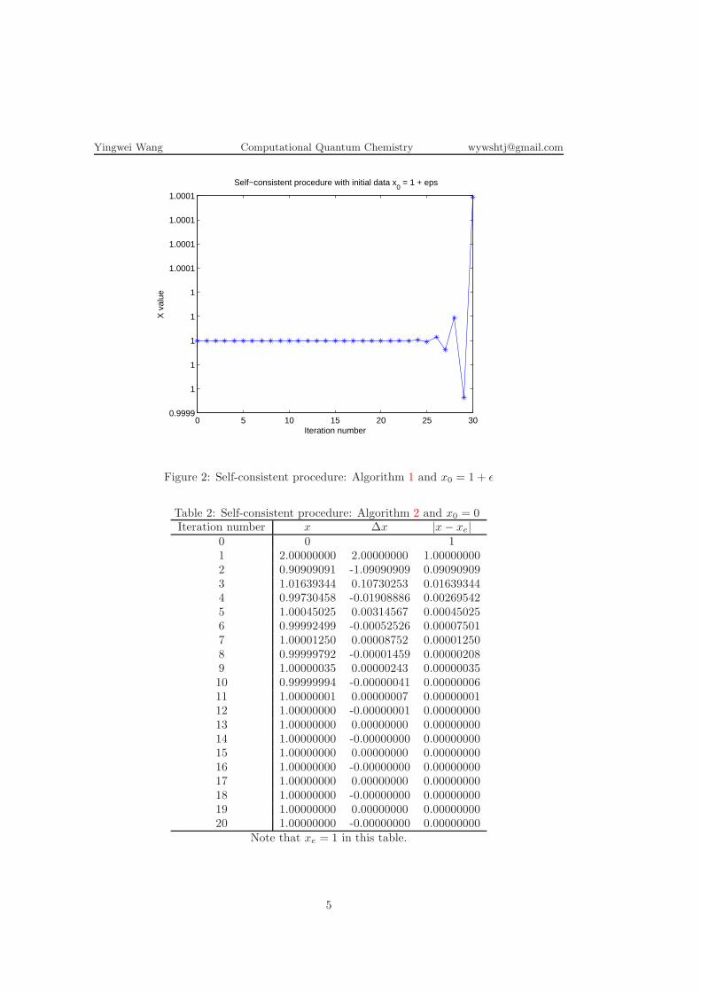
In order to find the solution x = 1, we need to rewrite the Eq.(3.2) in other forms. Forexample,
x ∗A(x) = B(x), A(x) := 5x+ 1, B(x) := 4x+ 2. (3.5)
The iteration scheme associated with (3.5) is shown in Algorithm 2.
Algorithm 2 Self consistent procedure with (3.5)
1: Initial guess x0.2: for k = 0, 1, 2, · · · do3: Solve xk+1 from the equation
xk+1 =4xk + 2
5xk + 1. (3.6)
4: Compute the ∆x = xk+1 − xk. If |∆x| < ǫ, then stop.5: end for
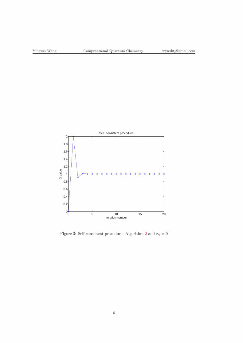
The numerical results for Algorithm 2 with x0 = 0 is shown in Table 2 and Fig.3.
4
Yingwei Wang Computational Quantum Chemistry [email protected]
0 5 10 15 20 25 300.9999
1
1
1
1
1
1.0001
1.0001
1.0001
1.0001
Self−consistent procedure with initial data x0 = 1 + eps
Iteration number
X v
alue
Figure 2: Self-consistent procedure: Algorithm 1 and x0 = 1 + ǫ
Table 2: Self-consistent procedure: Algorithm 2 and x0 = 0Iteration number x ∆x |x− xe|
0 0 11 2.00000000 2.00000000 1.000000002 0.90909091 -1.09090909 0.090909093 1.01639344 0.10730253 0.016393444 0.99730458 -0.01908886 0.002695425 1.00045025 0.00314567 0.000450256 0.99992499 -0.00052526 0.000075017 1.00001250 0.00008752 0.000012508 0.99999792 -0.00001459 0.000002089 1.00000035 0.00000243 0.0000003510 0.99999994 -0.00000041 0.0000000611 1.00000001 0.00000007 0.0000000112 1.00000000 -0.00000001 0.0000000013 1.00000000 0.00000000 0.0000000014 1.00000000 -0.00000000 0.0000000015 1.00000000 0.00000000 0.0000000016 1.00000000 -0.00000000 0.0000000017 1.00000000 0.00000000 0.0000000018 1.00000000 -0.00000000 0.0000000019 1.00000000 0.00000000 0.0000000020 1.00000000 -0.00000000 0.00000000
Note that xe = 1 in this table.
5
Yingwei Wang Computational Quantum Chemistry [email protected]
0 5 10 15 200
0.2
0.4
0.6
0.8
1
1.2
1.4
1.6
1.8
2Self−consistent procedure
Iteration number
X v
alue
Figure 3: Self-consistent procedure: Algorithm 2 and x0 = 0
6
Yingwei Wang Computational Quantum Chemistry [email protected]
Purdue University
CHM 67300
Computational Quantum Chemistry
HOMEWORK
Yingwei Wang
September 13, 2013
Homework set 3
Notations
(ij|kl) =
∫dr1dr2ψ
∗
i (r1)ψj(r1)r−1
12ψ∗
k(r2)ψl(r2), (0.1)
〈ij|kl〉 =
∫dr1dr2ψ
∗
i (r1)ψ∗
j (r2)r−1
12ψk(r1)ψl(r2), (0.2)
Jij = (ii|jj) = 〈ij|ij〉, called ’coulomb integral’ (0.3)
Kij = (ij|ji) = 〈ij|ji〉, called ’exchange integral’. (0.4)
1 Coulomb and exchange integrals
Problem: Prove the following properties of coulomb and exchange integrals:
Jii = Kii, (1.1)
J∗
ij = Jij , (1.2)
K∗
ij = Kij , (1.3)
Jij = Jji, (1.4)
Kij = Kji. (1.5)
Proof. According to the notations (0.1)-(0.4), it is easy to know the following.
Jii = (ii|ii) = Kii;
J∗
ij = (ii|jj) = Jij ;
K∗
ij = (ji|ij),
=
∫dr1dr2ψ
∗
j (r1)ψi(r1)r−1
12ψ∗
i (r2)ψj(r2),
=
∫dr1dr2ψ
∗
j (r2)ψi(r2)r−1
12ψ∗
i (r1)ψj(r1),
=
∫dr1dr2ψ
∗
i (r1)ψj(r1)r−1
12ψ∗
j (r2)ψi(r2),
= (ij|ji) = Kij;
1
Yingwei Wang Computational Quantum Chemistry [email protected]
Jij = (ii|jj),
=
∫dr1dr2ψ
∗
i (r1)ψi(r1)r−1
12ψ∗
j (r2)ψj(r2),
=
∫dr1dr2ψ
∗
i (r2)ψi(r2)r−1
12ψ∗
j (r1)ψj(r1),
=
∫dr1dr2ψ
∗
j (r1)ψj(r1)r−1
12ψ∗
i (r2)ψi(r2),
= (jj|ii) = Jji;
Kij = (ij|ji),
=
∫dr1dr2ψ
∗
i (r1)ψj(r1)r−1
12ψ∗
j (r2)ψi(r2),
=
∫dr1dr2ψ
∗
i (r2)ψj(r2)r−1
12ψ∗
j (r1)ψi(r1),
=
∫dr1dr2ψ
∗
j (r1)ψi(r1)r−1
12ψ∗
i (r2)ψj(r2),
= (ji|ij) = Kji.
2 Real spatial orbitals
Problem: Show that for real spatial obitals,
Kij = (ij|ij) = (ji|ji) = 〈ii|jj〉 = 〈jj|ii〉. (2.1)
Proof. For real spatial obitals, we have
Kij =
∫dr1dr2ψi(r1)ψj(r1)r
−1
12ψj(r2)ψi(r2),
=
∫dr1dr2ψi(r1)ψj(r1)r
−1
12ψi(r2)ψj(r2) = (ij|ij),
=
∫dr1dr2ψj(r1)ψi(r1)r
−1
12ψj(r2)ψi(r2) = (ji|ji),
=
∫dr1dr2ψi(r1)ψi(r2)r
−1
12ψj(r1)ψj(r2) = 〈ii|jj〉,
=
∫dr1dr2ψj(r1)ψj(r2)r
−1
12ψi(r1)ψi(r2) = 〈jj|ii〉.
2
Yingwei Wang Computational Quantum Chemistry [email protected]
3 Energy determinants
Problem: Verify the energies of the determinants shown in Fig.1 by inspection.
a. h11 + h22 + J12 −K12,
b. h11 + h22 + J12,
c. 2h11 + J11,
d. 2h2 + J22,
e. 2h11 + h22 + J11 + 2J12 −K12,
f. 2h22 + h11 + J22 + 2J12 −K12,
g. 2h11 + 2h22 + J11 + J22 + 4J12 − 2K12.
Figure 1: Energy determinants
Solution: Please see Table 1.
Table 1: Interpretation of determinantal energiesNumber one-electron Coulomb Exchange
a h11 + h22 J12 −K12
b h11 + h22 J12 0c 2h11 J11 0d 2h2 J22 0e 2h11 + h22 J11 + 2J12 −K12
f 2h22 + h11 J22 + 2J12 −K12
g 2h11 + 2h22 J11 + J22 + 4J12 −2K12
3
Yingwei Wang Computational Quantum Chemistry [email protected]
Purdue University
CHM 67300
Computational Quantum Chemistry
HOMEWORK
Yingwei Wang
October 4, 2013
Homework set 4
1 Basis sets
Question: Determine the total number of basis functions and primitive basis functionsfor STO-3G, 6-31G, 6-31G**, and 6-311(+,+)G** calculations of methane (CH4). Writethe contraction scheme in general notations for each basis (Szabo & Ostlund, chapter 3.6).Assume that pure angular momentum (5d,7f etc functions) polarization functions are used.
Answer:
1. The STO-3G basis set for methane consists of one 1s orbital on each H atom and a1s, 2s, and set of three 2p orbitals on C. See Tables 1-3 for details. The contractionscheme in general notations is (6s3p/3s)[2s1p/1s].
Table 1: STO-3G: Carbon atom1s 2s 2p(3) Total
No. Basis Functions 1 1 3 5No. Gaussians for each orbital 3 3 3
No. Primitives 3 3 9 15
Table 2: STO-3G: Hydrogen atom1s Total
No. Basis Functions 1 1No. Gaussians for each orbital 3
No. Primitives 3 3
Table 3: STO-3G: Methane moleculeNo. Basis Functions 5 + 1× 4 = 9
No. Primitives 15 + 3× 4 = 27
2. The 6-31G basis set is a split valence double zeta basis set. For hydrogen atom, a splitvalence double zeta basis consists of two 1s orbitals, denoted 1s and 1s’. Note that forthe H atom, because the 1s electron is considered the valence shell a double zeta basisset is used. For the carbon atom, a split valence double zeta basis set consists of asingle 1s orbital, along with two 2s and two each of 2px, 2py, and 2pz orbitals, denotedas 1s, 2s, 2s’, 2p(3) and 2p’(3). See Tables 4-6 for details. The contraction scheme ingeneral notations is (10s4p/4s)[3s2p/2s].
1
Yingwei Wang Computational Quantum Chemistry [email protected]
Table 4: 6-31G: Carbon atom1s 2s 2s’ 2p(3) 2p’(3) Total
No. Basis Functions 1 1 1 3 3 9No. Gaussians for each orbital 6 3 1 3 1
No. Primitives 6 3 1 9 3 22
Table 5: 6-31G: Hydrogen atom1s 1s’ Total
No. Basis Functions 1 1 2No. Gaussians for each orbital 3 1
No. Primitives 3 1 4
Table 6: 6-31G: Methane moleculeNo. Basis Functions 9 + 2× 4 = 17
No. Primitives 22 + 4× 4 = 38
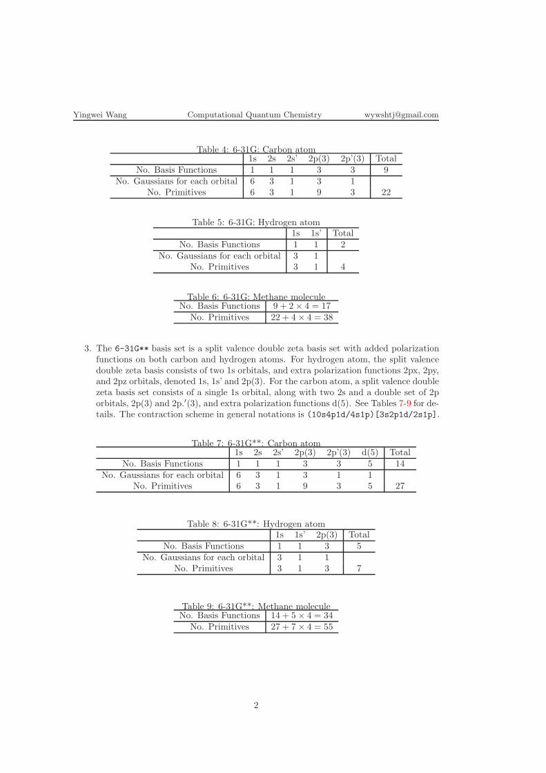
3. The 6-31G** basis set is a split valence double zeta basis set with added polarizationfunctions on both carbon and hydrogen atoms. For hydrogen atom, the split valencedouble zeta basis consists of two 1s orbitals, and extra polarization functions 2px, 2py,and 2pz orbitals, denoted 1s, 1s’ and 2p(3). For the carbon atom, a split valence doublezeta basis set consists of a single 1s orbital, along with two 2s and a double set of 2porbitals, 2p(3) and 2p.′(3), and extra polarization functions d(5). See Tables 7-9 for de-tails. The contraction scheme in general notations is (10s4p1d/4s1p)[3s2p1d/2s1p].
Table 7: 6-31G**: Carbon atom1s 2s 2s’ 2p(3) 2p’(3) d(5) Total
No. Basis Functions 1 1 1 3 3 5 14No. Gaussians for each orbital 6 3 1 3 1 1
No. Primitives 6 3 1 9 3 5 27
Table 8: 6-31G**: Hydrogen atom1s 1s’ 2p(3) Total
No. Basis Functions 1 1 3 5No. Gaussians for each orbital 3 1 1
No. Primitives 3 1 3 7
Table 9: 6-31G**: Methane moleculeNo. Basis Functions 14 + 5× 4 = 34
No. Primitives 27 + 7× 4 = 55
2
Yingwei Wang Computational Quantum Chemistry [email protected]
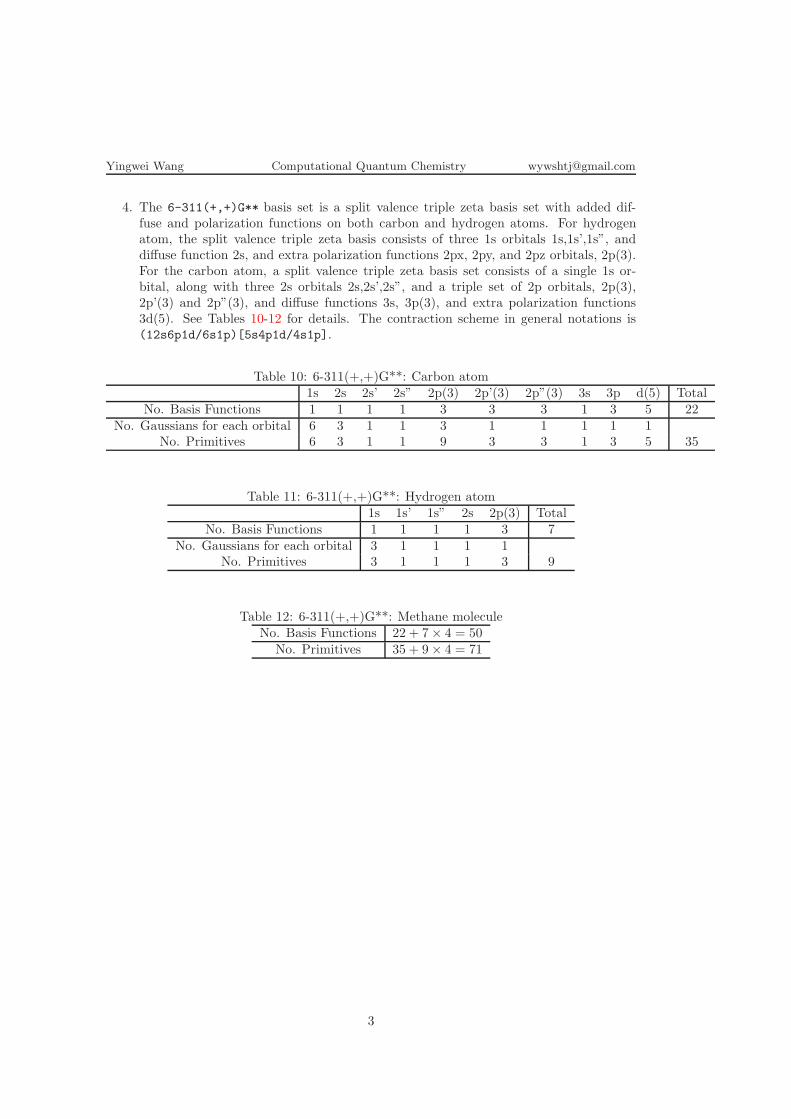
4. The 6-311(+,+)G** basis set is a split valence triple zeta basis set with added dif-fuse and polarization functions on both carbon and hydrogen atoms. For hydrogenatom, the split valence triple zeta basis consists of three 1s orbitals 1s,1s’,1s”, anddiffuse function 2s, and extra polarization functions 2px, 2py, and 2pz orbitals, 2p(3).For the carbon atom, a split valence triple zeta basis set consists of a single 1s or-bital, along with three 2s orbitals 2s,2s’,2s”, and a triple set of 2p orbitals, 2p(3),2p’(3) and 2p”(3), and diffuse functions 3s, 3p(3), and extra polarization functions3d(5). See Tables 10-12 for details. The contraction scheme in general notations is(12s6p1d/6s1p)[5s4p1d/4s1p].
Table 10: 6-311(+,+)G**: Carbon atom1s 2s 2s’ 2s” 2p(3) 2p’(3) 2p”(3) 3s 3p d(5) Total
No. Basis Functions 1 1 1 1 3 3 3 1 3 5 22No. Gaussians for each orbital 6 3 1 1 3 1 1 1 1 1
No. Primitives 6 3 1 1 9 3 3 1 3 5 35
Table 11: 6-311(+,+)G**: Hydrogen atom1s 1s’ 1s” 2s 2p(3) Total
No. Basis Functions 1 1 1 1 3 7No. Gaussians for each orbital 3 1 1 1 1
No. Primitives 3 1 1 1 3 9
Table 12: 6-311(+,+)G**: Methane moleculeNo. Basis Functions 22 + 7× 4 = 50
No. Primitives 35 + 9× 4 = 71
3
Yingwei Wang Computational Quantum Chemistry [email protected]
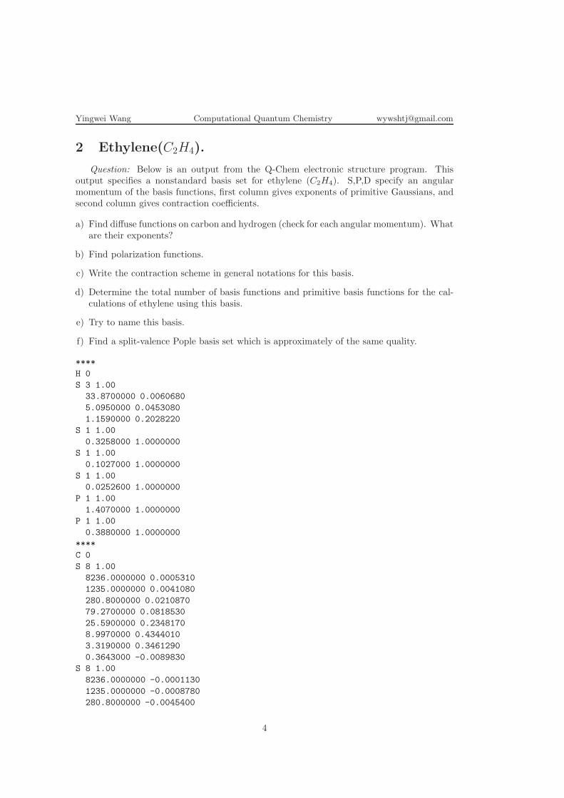
2 Ethylene(C2H4).
Question: Below is an output from the Q-Chem electronic structure program. Thisoutput specifies a nonstandard basis set for ethylene (C2H4). S,P,D specify an angularmomentum of the basis functions, first column gives exponents of primitive Gaussians, andsecond column gives contraction coefficients.
a) Find diffuse functions on carbon and hydrogen (check for each angular momentum). Whatare their exponents?
b) Find polarization functions.
c) Write the contraction scheme in general notations for this basis.
d) Determine the total number of basis functions and primitive basis functions for the cal-culations of ethylene using this basis.
e) Try to name this basis.
f) Find a split-valence Pople basis set which is approximately of the same quality.
****
H 0
S 3 1.00
33.8700000 0.0060680
5.0950000 0.0453080
1.1590000 0.2028220
S 1 1.00
0.3258000 1.0000000
S 1 1.00
0.1027000 1.0000000
S 1 1.00
0.0252600 1.0000000
P 1 1.00
1.4070000 1.0000000
P 1 1.00
0.3880000 1.0000000
****
C 0
S 8 1.00
8236.0000000 0.0005310
1235.0000000 0.0041080
280.8000000 0.0210870
79.2700000 0.0818530
25.5900000 0.2348170
8.9970000 0.4344010
3.3190000 0.3461290
0.3643000 -0.0089830
S 8 1.00
8236.0000000 -0.0001130
1235.0000000 -0.0008780
280.8000000 -0.0045400
4
Yingwei Wang Computational Quantum Chemistry [email protected]
79.2700000 -0.0181330
25.5900000 -0.0557600
8.9970000 -0.1268950
3.3190000 -0.1703520
0.3643000 0.5986840
S 1 1.00
0.9059000 1.0000000
S 1 1.00
0.1285000 1.0000000
S 1 1.00
0.0440200 1.0000000
P 3 1.00
18.7100000 0.0140310
4.1330000 0.0868660
1.2000000 0.2902160
P 1 1.00
0.3827000 1.0000000
P 1 1.00
0.1209000 1.0000000
P 1 1.00
0.0356900 1.0000000
D 1 1.00
1.0970000 1.0000000
D 1 1.00
0.3180000 1.0000000
****
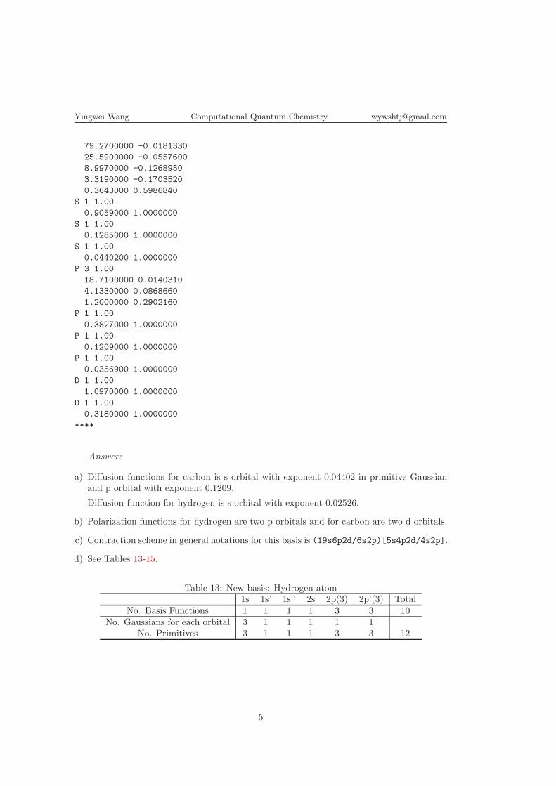
Answer:
a) Diffusion functions for carbon is s orbital with exponent 0.04402 in primitive Gaussianand p orbital with exponent 0.1209.
Diffusion function for hydrogen is s orbital with exponent 0.02526.
b) Polarization functions for hydrogen are two p orbitals and for carbon are two d orbitals.
c) Contraction scheme in general notations for this basis is (19s6p2d/6s2p)[5s4p2d/4s2p].
d) See Tables 13-15.
Table 13: New basis: Hydrogen atom1s 1s’ 1s” 2s 2p(3) 2p’(3) Total
No. Basis Functions 1 1 1 1 3 3 10No. Gaussians for each orbital 3 1 1 1 1 1
No. Primitives 3 1 1 1 3 3 12
5
Yingwei Wang Computational Quantum Chemistry [email protected]
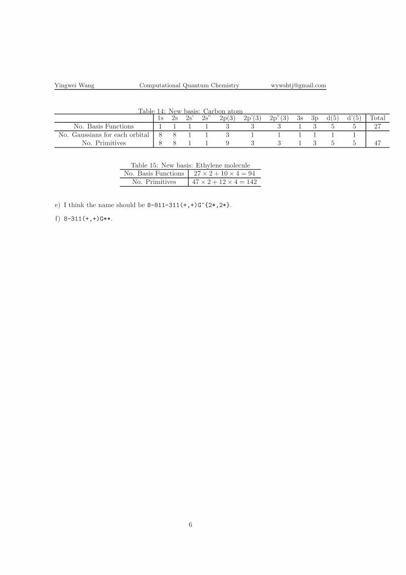
Table 14: New basis: Carbon atom1s 2s 2s’ 2s” 2p(3) 2p’(3) 2p”(3) 3s 3p d(5) d’(5) Total
No. Basis Functions 1 1 1 1 3 3 3 1 3 5 5 27No. Gaussians for each orbital 8 8 1 1 3 1 1 1 1 1 1
No. Primitives 8 8 1 1 9 3 3 1 3 5 5 47
Table 15: New basis: Ethylene moleculeNo. Basis Functions 27× 2 + 10× 4 = 94
No. Primitives 47× 2 + 12× 4 = 142
e) I think the name should be 8-811-311(+,+)G^{2*,2*}.
f) 8-311(+,+)G**.
6
Yingwei Wang Computational Quantum Chemistry [email protected]
Purdue University
CHM 67300
Computational Quantum Chemistry
LAB REPOROT
Yingwei Wang
October 15, 2013
Lab 1
1 Summarize the results you obtained for your (neutral)molecule
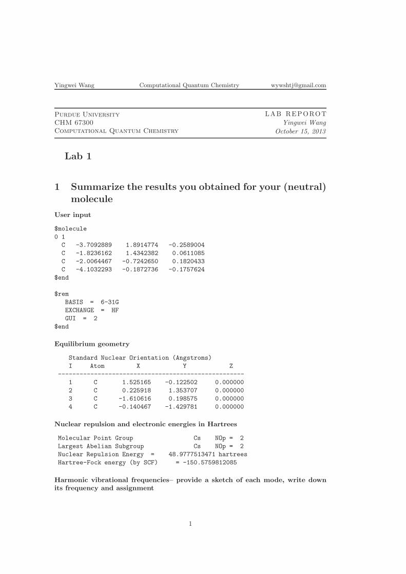
User input
$molecule
0 1
C -3.7092889 1.8914774 -0.2589004
C -1.8236162 1.4342382 0.0611085
C -2.0064467 -0.7242650 0.1820433
C -4.1032293 -0.1872736 -0.1757624
$end
$rem
BASIS = 6-31G
EXCHANGE = HF
GUI = 2
$end
Equilibrium geometry
Standard Nuclear Orientation (Angstroms)
I Atom X Y Z
----------------------------------------------------
1 C 1.525165 -0.122502 0.000000
2 C 0.225918 1.353707 0.000000
3 C -1.610616 0.198575 0.000000
4 C -0.140467 -1.429781 0.000000
Nuclear repulsion and electronic energies in Hartrees
Molecular Point Group Cs NOp = 2
Largest Abelian Subgroup Cs NOp = 2
Nuclear Repulsion Energy = 48.9777513471 hartrees
Hartree-Fock energy (by SCF) = -150.5759812085
Harmonic vibrational frequencies– provide a sketch of each mode, write downits frequency and assignment
1
Yingwei Wang Computational Quantum Chemistry [email protected]
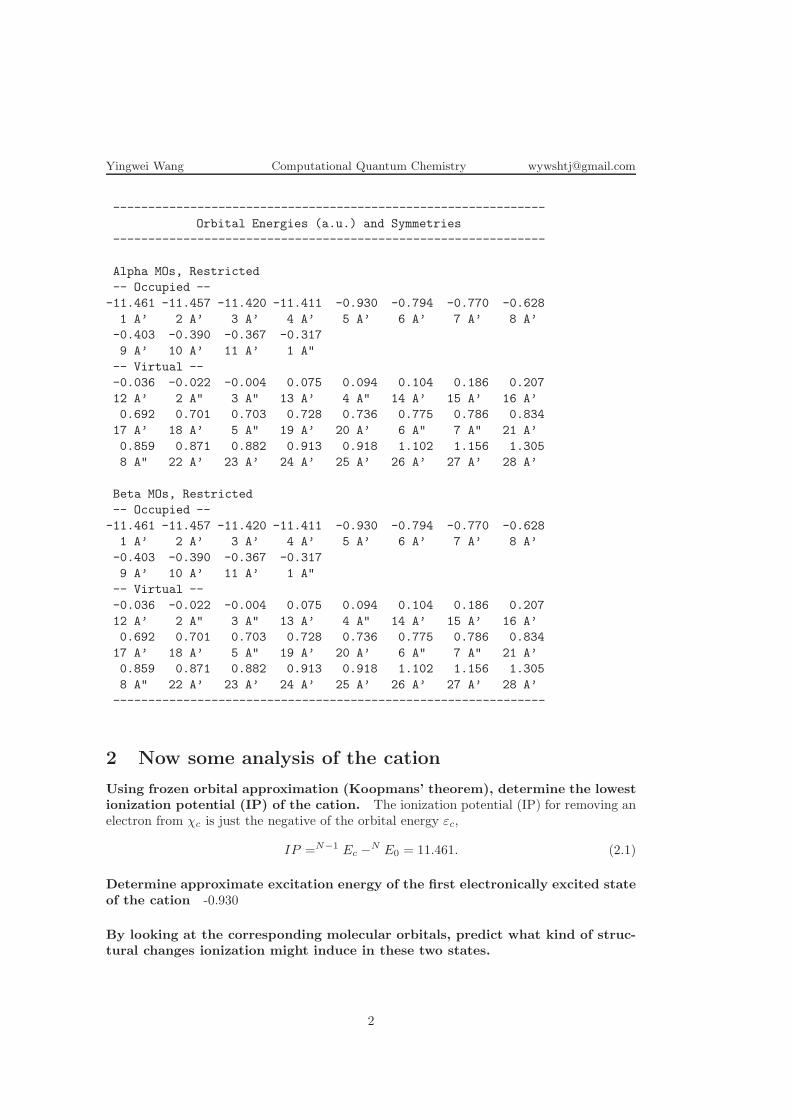
--------------------------------------------------------------
Orbital Energies (a.u.) and Symmetries
--------------------------------------------------------------
Alpha MOs, Restricted
-- Occupied --
-11.461 -11.457 -11.420 -11.411 -0.930 -0.794 -0.770 -0.628
1 A’ 2 A’ 3 A’ 4 A’ 5 A’ 6 A’ 7 A’ 8 A’
-0.403 -0.390 -0.367 -0.317
9 A’ 10 A’ 11 A’ 1 A"
-- Virtual --
-0.036 -0.022 -0.004 0.075 0.094 0.104 0.186 0.207
12 A’ 2 A" 3 A" 13 A’ 4 A" 14 A’ 15 A’ 16 A’
0.692 0.701 0.703 0.728 0.736 0.775 0.786 0.834
17 A’ 18 A’ 5 A" 19 A’ 20 A’ 6 A" 7 A" 21 A’
0.859 0.871 0.882 0.913 0.918 1.102 1.156 1.305
8 A" 22 A’ 23 A’ 24 A’ 25 A’ 26 A’ 27 A’ 28 A’
Beta MOs, Restricted
-- Occupied --
-11.461 -11.457 -11.420 -11.411 -0.930 -0.794 -0.770 -0.628
1 A’ 2 A’ 3 A’ 4 A’ 5 A’ 6 A’ 7 A’ 8 A’
-0.403 -0.390 -0.367 -0.317
9 A’ 10 A’ 11 A’ 1 A"
-- Virtual --
-0.036 -0.022 -0.004 0.075 0.094 0.104 0.186 0.207
12 A’ 2 A" 3 A" 13 A’ 4 A" 14 A’ 15 A’ 16 A’
0.692 0.701 0.703 0.728 0.736 0.775 0.786 0.834
17 A’ 18 A’ 5 A" 19 A’ 20 A’ 6 A" 7 A" 21 A’
0.859 0.871 0.882 0.913 0.918 1.102 1.156 1.305
8 A" 22 A’ 23 A’ 24 A’ 25 A’ 26 A’ 27 A’ 28 A’
--------------------------------------------------------------
2 Now some analysis of the cation
Using frozen orbital approximation (Koopmans’ theorem), determine the lowestionization potential (IP) of the cation. The ionization potential (IP) for removing anelectron from χc is just the negative of the orbital energy εc,
IP =N−1 Ec −N E0 = 11.461. (2.1)
Determine approximate excitation energy of the first electronically excited stateof the cation -0.930
By looking at the corresponding molecular orbitals, predict what kind of struc-tural changes ionization might induce in these two states.
2

Yingwei Wang Computational Quantum Chemistry [email protected]
Calculate the lowest IP as the Hartree–Fock energy difference between the neu-tral and the cation. Compare this so-called ∆EIP with Koopmans IP. Explainthe difference
3
Yingwei Wang Computational Quantum Chemistry [email protected]
Purdue University
CHM 67300
Computational Quantum Chemistry
LAB REPOROT
Yingwei Wang
October 29, 2013
Lab 2: Bond-breaking in H2
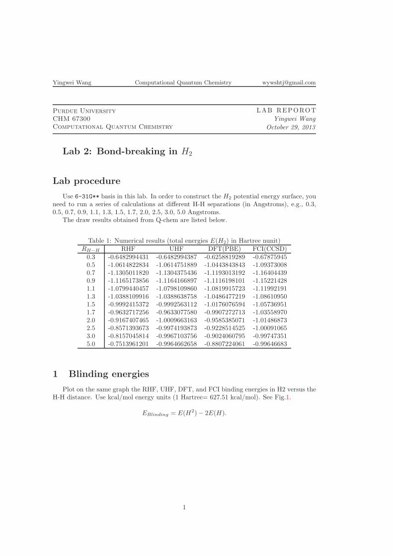
Lab procedure
Use 6-31G** basis in this lab. In order to construct the H2 potential energy surface, youneed to run a series of calculations at different H-H separations (in Angstroms), e.g., 0.3,0.5, 0.7, 0.9, 1.1, 1.3, 1.5, 1.7, 2.0, 2.5, 3.0, 5.0 Angstroms.
The draw results obtained from Q-chem are listed below.
Table 1: Numerical results (total energies E(H2) in Hartree nunit)RH−H RHF UHF DFT(PBE) FCI(CCSD)0.3 -0.6482994431 -0.6482994387 -0.6258819289 -0.678759450.5 -1.0614822834 -1.0614751889 -1.0443843843 -1.093730080.7 -1.1305011820 -1.1304375436 -1.1193013192 -1.164044390.9 -1.1165173856 -1.1164166897 -1.1116198101 -1.152214281.1 -1.0799440457 -1.0798109860 -1.0819915723 -1.119921911.3 -1.0388109916 -1.0388638758 -1.0486477219 -1.086109501.5 -0.9992415372 -0.9992563112 -1.0176076594 -1.057369511.7 -0.9632717256 -0.9633077580 -0.9907272713 -1.035589702.0 -0.9167407465 -1.0009663163 -0.9585385071 -1.014868732.5 -0.8571393673 -0.9974193873 -0.9228514525 -1.000910653.0 -0.8157045814 -0.9967103756 -0.9024060795 -0.997473515.0 -0.7513961201 -0.9964662658 -0.8807224061 -0.99646683
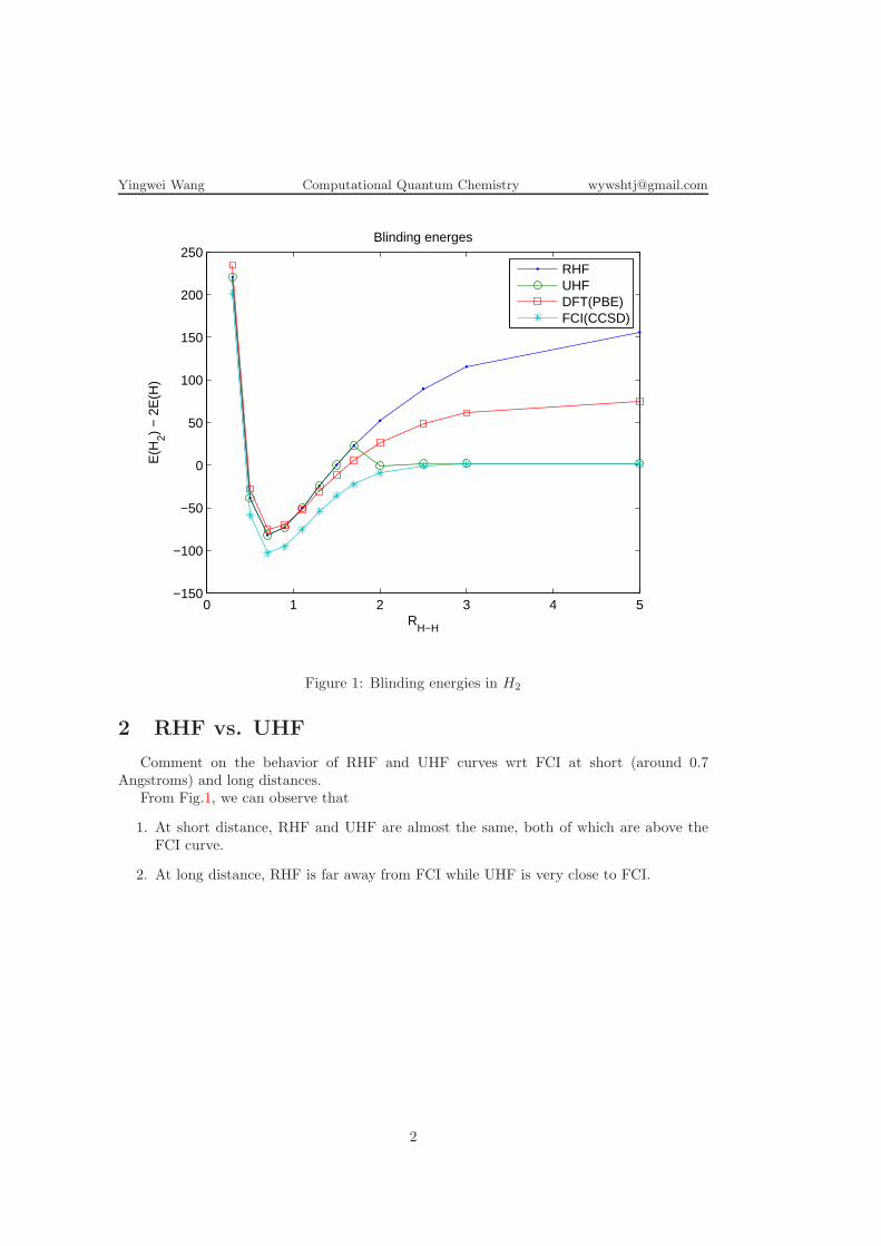
1 Blinding energies
Plot on the same graph the RHF, UHF, DFT, and FCI binding energies in H2 versus theH-H distance. Use kcal/mol energy units (1 Hartree= 627.51 kcal/mol). See Fig.1.
EBlinding = E(H2)− 2E(H).
1
Yingwei Wang Computational Quantum Chemistry [email protected]
0 1 2 3 4 5−150
−100
−50
0
50
100
150
200
250Blinding energes
RH−H
E(H
2) −
2E
(H)
RHFUHFDFT(PBE)FCI(CCSD)
Figure 1: Blinding energies in H2
2 RHF vs. UHF
Comment on the behavior of RHF and UHF curves wrt FCI at short (around 0.7Angstroms) and long distances.
From Fig.1, we can observe that
1. At short distance, RHF and UHF are almost the same, both of which are above theFCI curve.
2. At long distance, RHF is far away from FCI while UHF is very close to FCI.
2
Yingwei Wang Computational Quantum Chemistry [email protected]
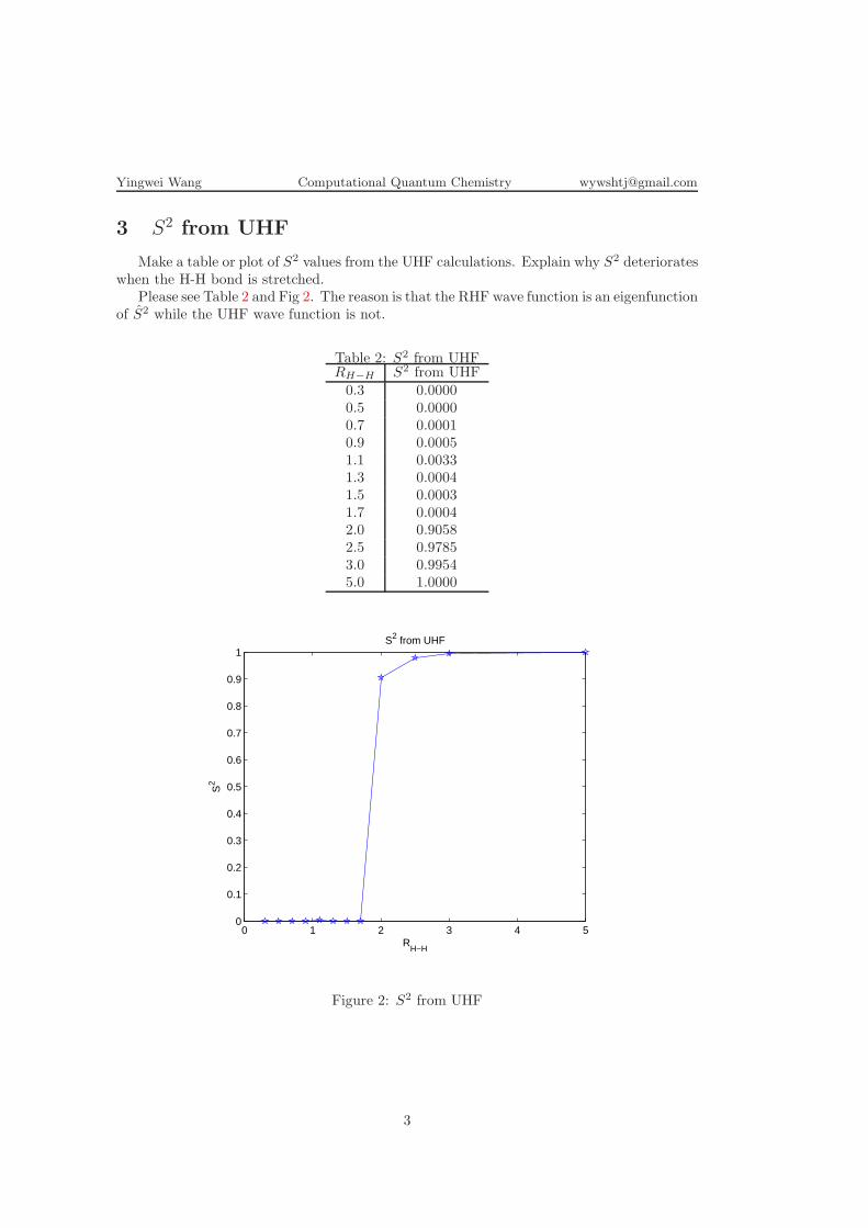
3 S2 from UHF
Make a table or plot of S2 values from the UHF calculations. Explain why S2 deteriorateswhen the H-H bond is stretched.
Please see Table 2 and Fig 2. The reason is that the RHF wave function is an eigenfunctionof S2 while the UHF wave function is not.
Table 2: S2 from UHFRH−H S2 from UHF0.3 0.00000.5 0.00000.7 0.00010.9 0.00051.1 0.00331.3 0.00041.5 0.00031.7 0.00042.0 0.90582.5 0.97853.0 0.99545.0 1.0000
0 1 2 3 4 50
0.1
0.2
0.3
0.4
0.5
0.6
0.7
0.8
0.9
1S2 from UHF
RH−H
S2
Figure 2: S2 from UHF
3
Yingwei Wang Computational Quantum Chemistry [email protected]
4 HOMO and LUMO
Make a sketch of the first two H2 molecular orbitals (HOMO and LUMO) from yourRHF and UHF calculations at the equilibrium (0.7 Angstroms), 1.3, and 5.0 Angstroms.Comment on qualitative changes in the shape of the orbitals.
I do not know which part of the output is related to this problem.
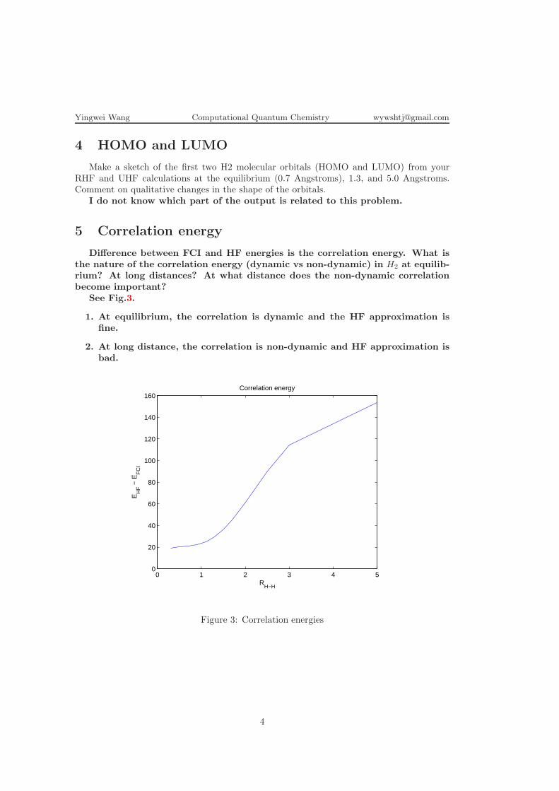
5 Correlation energy
Difference between FCI and HF energies is the correlation energy. What isthe nature of the correlation energy (dynamic vs non-dynamic) in H2 at equilib-rium? At long distances? At what distance does the non-dynamic correlationbecome important?
See Fig.3.
1. At equilibrium, the correlation is dynamic and the HF approximation isfine.
2. At long distance, the correlation is non-dynamic and HF approximation isbad.
0 1 2 3 4 50
20
40
60
80
100
120
140
160Correlation energy
RH−H
EH
F −
EF
CI
Figure 3: Correlation energies
4

Yingwei Wang Computational Quantum Chemistry [email protected]
6 DFT
Comment on the behavior of DFT at equilibrium and long distances. Whatis a reason of DFT failure for bond-breaking?
1. At equilibrium, the DFT is better than RHF and UHF.
2. At long distance, the DFT is worse than UHF but better than RHF.
5
Yingwei Wang Computational Quantum Chemistry [email protected]
Purdue University
CHM 67300
Computational Quantum Chemistry
LAB REPOROT
Yingwei Wang
November 21, 2013
Lab 3: Extrapolation techniques foraccurate thermochemistry
Contents
0 Lab procedure 20.1 Geometry optimization . . . . . . . . . . . . . . . . . . . . . . . . . . . 20.2 Energies calculation . . . . . . . . . . . . . . . . . . . . . . . . . . . . . 3
1 HF energies 7
2 Correlation and total energies 8
3 Bond dissociation energies 10
4 Further discussion 114.1 Convergence rates . . . . . . . . . . . . . . . . . . . . . . . . . . . . . . 114.2 MP2 CBS extrapolations . . . . . . . . . . . . . . . . . . . . . . . . . . 114.3 Accuracy and reliability . . . . . . . . . . . . . . . . . . . . . . . . . . 114.4 Energy additivity scheme . . . . . . . . . . . . . . . . . . . . . . . . . . 124.5 New CCSD(T) BDE values . . . . . . . . . . . . . . . . . . . . . . . . 124.6 Efficiency . . . . . . . . . . . . . . . . . . . . . . . . . . . . . . . . . . 12
1
Yingwei Wang Computational Quantum Chemistry [email protected]
0 Lab procedure
0.1 Geometry optimization
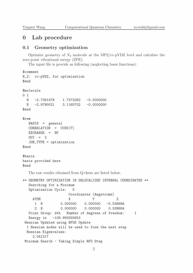
Optimize geometry of N2 molecule at the MP2/cc-pVDZ level and calculate thezero-point vibrational energy (ZPE).
The input file is provide as following (neglecting basis functions):
$comment
N_2: cc-pVDZ, for optimization
$end
$molecule
0 1
N -2.7391478 1.7372082 -0.0000000
N -2.9790021 3.1165702 -0.0000000
$end
$rem
BASIS = general
CORRELATION = CCSD(T)
EXCHANGE = HF
GUI = 2
JOB_TYPE = optimization
$end
$basis
basis provided here
$end
The raw results obtained from Q-chem are listed below.
** GEOMETRY OPTIMIZATION IN DELOCALIZED INTERNAL COORDINATES **
Searching for a Minimum
Optimization Cycle: 5
Coordinates (Angstroms)
ATOM X Y Z
1 N 0.000000 0.000000 -0.538684
2 N 0.000000 0.000000 0.538684
Point Group: d*h Number of degrees of freedom: 1
Energy is -108.955555653
Hessian Updated using BFGS Update
1 Hessian modes will be used to form the next step
Hessian Eigenvalues:
2.041217
Minimum Search - Taking Simple RFO Step
2
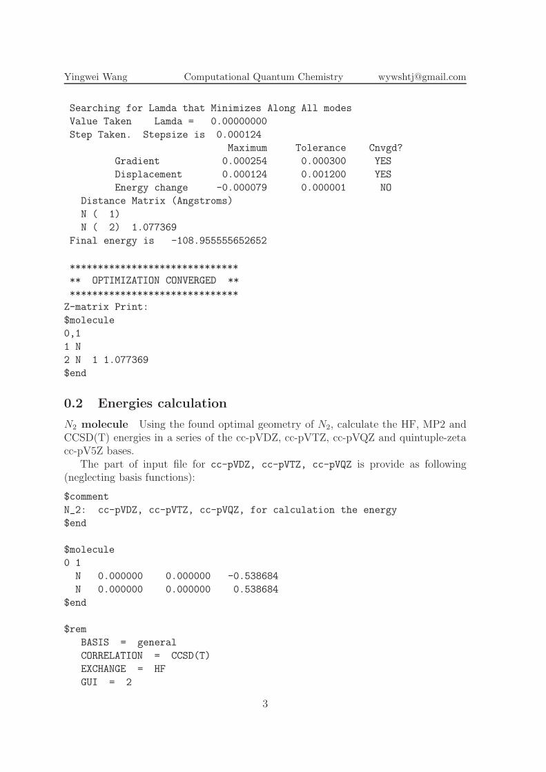
Yingwei Wang Computational Quantum Chemistry [email protected]
Searching for Lamda that Minimizes Along All modes
Value Taken Lamda = 0.00000000
Step Taken. Stepsize is 0.000124
Maximum Tolerance Cnvgd?
Gradient 0.000254 0.000300 YES
Displacement 0.000124 0.001200 YES
Energy change -0.000079 0.000001 NO
Distance Matrix (Angstroms)
N ( 1)
N ( 2) 1.077369
Final energy is -108.955555652652
******************************
** OPTIMIZATION CONVERGED **
******************************
Z-matrix Print:
$molecule
0,1
1 N
2 N 1 1.077369
$end
0.2 Energies calculation
N2 molecule Using the found optimal geometry of N2, calculate the HF, MP2 andCCSD(T) energies in a series of the cc-pVDZ, cc-pVTZ, cc-pVQZ and quintuple-zetacc-pV5Z bases.
The part of input file for cc-pVDZ, cc-pVTZ, cc-pVQZ is provide as following(neglecting basis functions):
$comment
N_2: cc-pVDZ, cc-pVTZ, cc-pVQZ, for calculation the energy
$end
$molecule
0 1
N 0.000000 0.000000 -0.538684
N 0.000000 0.000000 0.538684
$end
$rem
BASIS = general
CORRELATION = CCSD(T)
EXCHANGE = HF
GUI = 2
3
Yingwei Wang Computational Quantum Chemistry [email protected]
$end
$basis
****
$end
@@@
...
The input file for cc-pV5Z is provide as following (neglecting basis functions):
$comment
N_2: cc-pV5Z,MP2, for calculation the energy
$end
$molecule
0 1
N 0.000000 0.000000 -0.538684
N 0.000000 0.000000 0.538684
$end
$rem
BASIS = general
CORRELATION = MP2
EXCHANGE = HF
JOB_TYPE = sp
mem_static = 200
$end
$basis
****
$end
Note that the basis sets cc-pVDZ, cc-pVTZ, cc-pVQZ and cc-pV5Z are down-loaded from the online basis set library [1] (choose Gaussian94 format).
The raw results obtained from Q-chem are listed below.
cc-pVDZ:
SCF energy = -108.95555877
MP2 energy = -109.26018891
CCSD correlation energy = -0.30860003
CCSD total energy = -109.26415880
CCSD(T) correlation energy = -0.01131523
CCSD(T) total energy = -109.27547403
CCSD T1^2 = 0.0025 T2^2 = 0.1094.
4
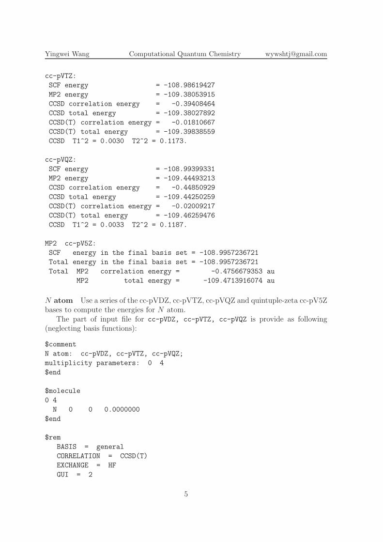
Yingwei Wang Computational Quantum Chemistry [email protected]
cc-pVTZ:
SCF energy = -108.98619427
MP2 energy = -109.38053915
CCSD correlation energy = -0.39408464
CCSD total energy = -109.38027892
CCSD(T) correlation energy = -0.01810667
CCSD(T) total energy = -109.39838559
CCSD T1^2 = 0.0030 T2^2 = 0.1173.
cc-pVQZ:
SCF energy = -108.99399331
MP2 energy = -109.44493213
CCSD correlation energy = -0.44850929
CCSD total energy = -109.44250259
CCSD(T) correlation energy = -0.02009217
CCSD(T) total energy = -109.46259476
CCSD T1^2 = 0.0033 T2^2 = 0.1187.
MP2 cc-pV5Z:
SCF energy in the final basis set = -108.9957236721
Total energy in the final basis set = -108.9957236721
Total MP2 correlation energy = -0.4756679353 au
MP2 total energy = -109.4713916074 au
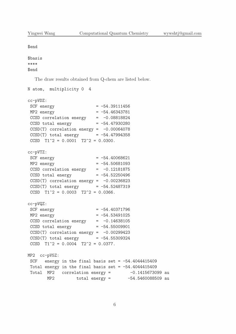
N atom Use a series of the cc-pVDZ, cc-pVTZ, cc-pVQZ and quintuple-zeta cc-pV5Zbases to compute the energies for N atom.
The part of input file for cc-pVDZ, cc-pVTZ, cc-pVQZ is provide as following(neglecting basis functions):
$comment
N atom: cc-pVDZ, cc-pVTZ, cc-pVQZ;
multiplicity parameters: 0 4
$end
$molecule
0 4
N 0 0 0.0000000
$end
$rem
BASIS = general
CORRELATION = CCSD(T)
EXCHANGE = HF
GUI = 2
5
Yingwei Wang Computational Quantum Chemistry [email protected]
$end
$basis
****
$end
The draw results obtained from Q-chem are listed below.
N atom, multiplicity 0 4
cc-pVDZ:
SCF energy = -54.39111456
MP2 energy = -54.46343781
CCSD correlation energy = -0.08818824
CCSD total energy = -54.47930280
CCSD(T) correlation energy = -0.00064078
CCSD(T) total energy = -54.47994358
CCSD T1^2 = 0.0001 T2^2 = 0.0300.
cc-pVTZ:
SCF energy = -54.40068621
MP2 energy = -54.50681093
CCSD correlation energy = -0.12181875
CCSD total energy = -54.52250496
CCSD(T) correlation energy = -0.00236823
CCSD(T) total energy = -54.52487319
CCSD T1^2 = 0.0003 T2^2 = 0.0366.
cc-pVQZ:
SCF energy = -54.40371796
MP2 energy = -54.53491025
CCSD correlation energy = -0.14638105
CCSD total energy = -54.55009901
CCSD(T) correlation energy = -0.00299423
CCSD(T) total energy = -54.55309324
CCSD T1^2 = 0.0004 T2^2 = 0.0377.
MP2 cc-pV5Z:
SCF energy in the final basis set = -54.4044415409
Total energy in the final basis set = -54.4044415409
Total MP2 correlation energy = -0.1415673099 au
MP2 total energy = -54.5460088509 au
6
Yingwei Wang Computational Quantum Chemistry [email protected]
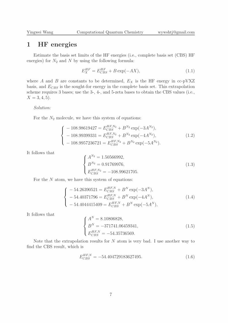
1 HF energies
Estimate the basis set limits of the HF energies (i.e., complete basis set (CBS) HFenergies) for N2 and N by using the following formula:
EHFX = EHF
CBS +B exp(−AX), (1.1)
where A and B are constants to be determined, EX is the HF energy in cc-pVXZbasis, and ECBS is the sought-for energy in the complete basis set. This extrapolationscheme requires 3 bases; use the 3-, 4-, and 5-zeta bases to obtain the CBS values (i.e.,X = 3, 4, 5).
Solution:
For the N2 molecule, we have this system of equations:
− 108.98619427 = EHF,N2
CBS +BN2 exp(−3AN2),
− 108.99399331 = EHF,N2
CBS +BN2 exp(−4AN2),
− 108.9957236721 = EHF,N2
CBS +BN2 exp(−5AN2).
(1.2)
It follows that
AN2 = 1.50566992,
BN2 = 0.91769976,
EHF,N2
CBS = −108.99621705.
(1.3)
For the N atom, we have this system of equations:
− 54.26390521 = EHF,NCBS +BN exp(−3AN ),
− 54.40371796 = EHF,NCBS +BN exp(−4AN ),
− 54.4044415409 = EHF,NCBS +BN exp(−5AN),
(1.4)
It follows that
AN = 8.10806828,
BN = −371741.06459341,
EHF,NCBS = −54.35736569.
(1.5)
Note that the extrapolation results for N atom is very bad. I use another way tofind the CBS result, which is
EHF,NCBS = −54.404729183627495. (1.6)
7
Yingwei Wang Computational Quantum Chemistry [email protected]
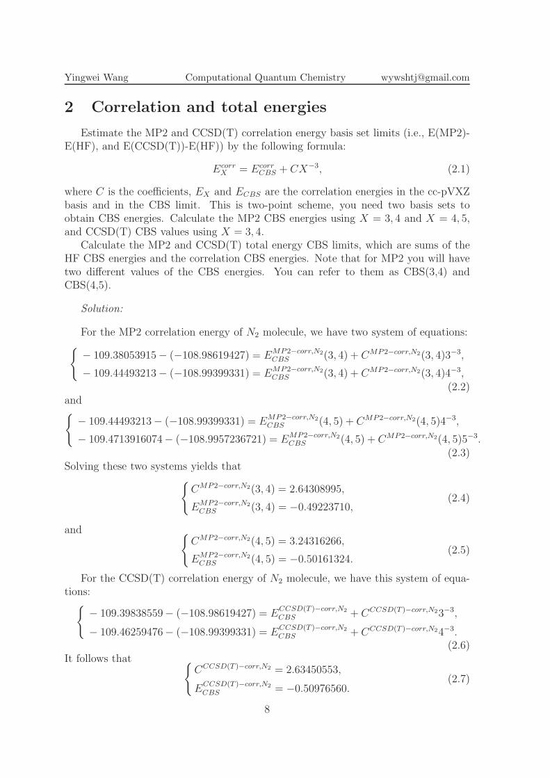
2 Correlation and total energies
Estimate the MP2 and CCSD(T) correlation energy basis set limits (i.e., E(MP2)-E(HF), and E(CCSD(T))-E(HF)) by the following formula:
EcorrX = Ecorr
CBS + CX−3, (2.1)
where C is the coefficients, EX and ECBS are the correlation energies in the cc-pVXZbasis and in the CBS limit. This is two-point scheme, you need two basis sets toobtain CBS energies. Calculate the MP2 CBS energies using X = 3, 4 and X = 4, 5,and CCSD(T) CBS values using X = 3, 4.
Calculate the MP2 and CCSD(T) total energy CBS limits, which are sums of theHF CBS energies and the correlation CBS energies. Note that for MP2 you will havetwo different values of the CBS energies. You can refer to them as CBS(3,4) andCBS(4,5).
Solution:
For the MP2 correlation energy of N2 molecule, we have two system of equations:{
− 109.38053915− (−108.98619427) = EMP2−corr,N2
CBS (3, 4) + CMP2−corr,N2(3, 4)3−3,
− 109.44493213− (−108.99399331) = EMP2−corr,N2
CBS (3, 4) + CMP2−corr,N2(3, 4)4−3,(2.2)
and{
− 109.44493213− (−108.99399331) = EMP2−corr,N2
CBS (4, 5) + CMP2−corr,N2(4, 5)4−3,
− 109.4713916074− (−108.9957236721) = EMP2−corr,N2
CBS (4, 5) + CMP2−corr,N2(4, 5)5−3.(2.3)
Solving these two systems yields that{
CMP2−corr,N2(3, 4) = 2.64308995,
EMP2−corr,N2
CBS (3, 4) = −0.49223710,(2.4)
and{
CMP2−corr,N2(4, 5) = 3.24316266,
EMP2−corr,N2
CBS (4, 5) = −0.50161324.(2.5)
For the CCSD(T) correlation energy of N2 molecule, we have this system of equa-tions:
{
− 109.39838559− (−108.98619427) = ECCSD(T )−corr,N2
CBS + CCCSD(T )−corr,N23−3,
− 109.46259476− (−108.99399331) = ECCSD(T )−corr,N2
CBS + CCCSD(T )−corr,N24−3.(2.6)
It follows that{
CCCSD(T )−corr,N2 = 2.63450553,
ECCSD(T )−corr,N2
CBS = −0.50976560.(2.7)
8
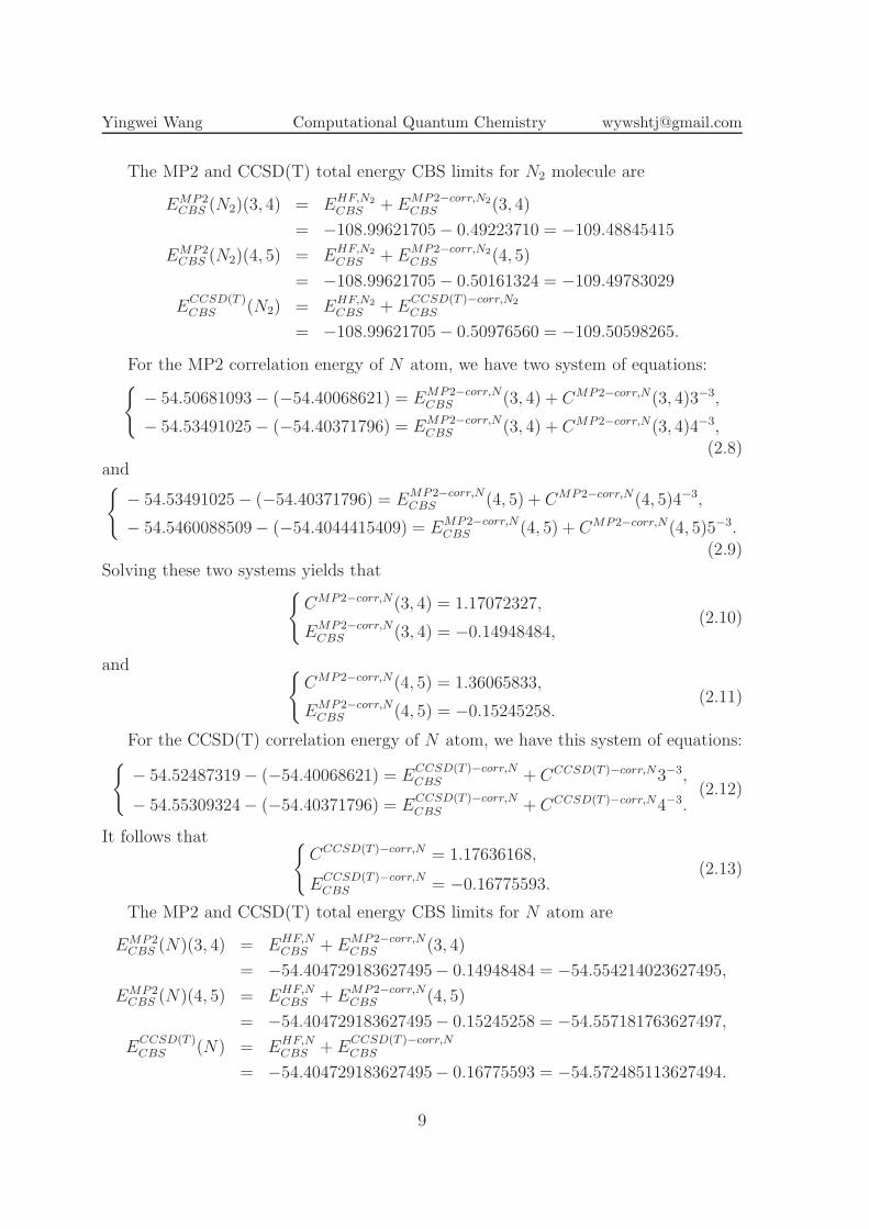
Yingwei Wang Computational Quantum Chemistry [email protected]
The MP2 and CCSD(T) total energy CBS limits for N2 molecule are
EMP2CBS (N2)(3, 4) = EHF,N2
CBS + EMP2−corr,N2
CBS (3, 4)
= −108.99621705− 0.49223710 = −109.48845415
EMP2CBS (N2)(4, 5) = EHF,N2
CBS + EMP2−corr,N2
CBS (4, 5)
= −108.99621705− 0.50161324 = −109.49783029
ECCSD(T )CBS (N2) = EHF,N2
CBS + ECCSD(T )−corr,N2
CBS
= −108.99621705− 0.50976560 = −109.50598265.
For the MP2 correlation energy of N atom, we have two system of equations:{
− 54.50681093− (−54.40068621) = EMP2−corr,NCBS (3, 4) + CMP2−corr,N(3, 4)3−3,
− 54.53491025− (−54.40371796) = EMP2−corr,NCBS (3, 4) + CMP2−corr,N(3, 4)4−3,
(2.8)and{
− 54.53491025− (−54.40371796) = EMP2−corr,NCBS (4, 5) + CMP2−corr,N(4, 5)4−3,
− 54.5460088509− (−54.4044415409) = EMP2−corr,NCBS (4, 5) + CMP2−corr,N(4, 5)5−3.
(2.9)Solving these two systems yields that
{
CMP2−corr,N(3, 4) = 1.17072327,
EMP2−corr,NCBS (3, 4) = −0.14948484,
(2.10)
and{
CMP2−corr,N(4, 5) = 1.36065833,
EMP2−corr,NCBS (4, 5) = −0.15245258.
(2.11)
For the CCSD(T) correlation energy of N atom, we have this system of equations:{
− 54.52487319− (−54.40068621) = ECCSD(T )−corr,N
CBS + CCCSD(T )−corr,N3−3,
− 54.55309324− (−54.40371796) = ECCSD(T )−corr,N
CBS + CCCSD(T )−corr,N4−3.(2.12)
It follows that{
CCCSD(T )−corr,N = 1.17636168,
ECCSD(T )−corr,N
CBS = −0.16775593.(2.13)
The MP2 and CCSD(T) total energy CBS limits for N atom are
EMP2CBS (N)(3, 4) = EHF,N
CBS + EMP2−corr,NCBS (3, 4)
= −54.404729183627495− 0.14948484 = −54.554214023627495,
EMP2CBS (N)(4, 5) = EHF,N
CBS + EMP2−corr,NCBS (4, 5)
= −54.404729183627495− 0.15245258 = −54.557181763627497,
ECCSD(T )CBS (N) = EHF,N
CBS + ECCSD(T )−corr,N
CBS
= −54.404729183627495− 0.16775593 = −54.572485113627494.
9
Yingwei Wang Computational Quantum Chemistry [email protected]
3 Bond dissociation energies
Calculate the bond dissociation energies (Ediss = E(N2)−2E(N)) by HF, MP2, andCCSD(T) in different basis sets. Calculate CBS-estimated bond dissociation energiesas a difference between CBS energies of N2 and N :
ECBSdiss = ECBS(N2)− 2ECBS((N). (3.1)
Use kcal/mol units for reporting bond dissociation energies. Note that 1Hatree =627.51kcal/mol.
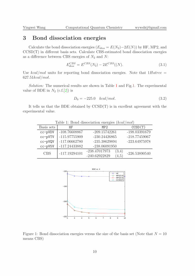
Solution: The numerical results are shown in Table 1 and Fig.1. The experimentalvalue of BDE in N2 (c.f.[2]) is
D0 = −225.0 kcal/mol. (3.2)
It tells us that the BDE obtained by CCSD(T) is in excellent agreement with theexperimental value.
Table 1: Bond dissociation energies (kcal/mol)Basis sets HF MP2 CCSD(T)
cc-pVDV -108.76608867 -209.15742261 -198.03391679cc-pVTV -115.97755909 -230.24426865 -218.77459067cc-pVQV -117.06662780 -235.38629894 -223.64975978cc-pV5V -117.24433882 -238.06091950
CBS -117.19294101-238.47017973 (3,4)
-226.53890540-240.62922829 (4,5)
2 3 4 5 6 7 8 9 10−250
−200
−150
−100BDE vs. X
HFMP2(3,4)MP2(4,5)CCSD(T)
Figure 1: Bond dissociation energies versus the size of the basis set (Note that N = 10means CBS)
10
Yingwei Wang Computational Quantum Chemistry [email protected]
4 Further discussion
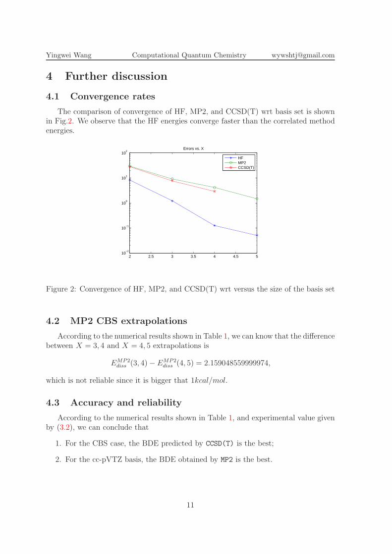
4.1 Convergence rates
The comparison of convergence of HF, MP2, and CCSD(T) wrt basis set is shownin Fig.2. We observe that the HF energies converge faster than the correlated methodenergies.
2 2.5 3 3.5 4 4.5 510
−2
10−1
100
101
102
Errors vs. X
HFMP2CCSD(T)
Figure 2: Convergence of HF, MP2, and CCSD(T) wrt versus the size of the basis set
4.2 MP2 CBS extrapolations
According to the numerical results shown in Table 1, we can know that the differencebetween X = 3, 4 and X = 4, 5 extrapolations is
EMP2diss (3, 4)− EMP2
diss (4, 5) = 2.159048559999974,
which is not reliable since it is bigger that 1kcal/mol.
4.3 Accuracy and reliability
According to the numerical results shown in Table 1, and experimental value givenby (3.2), we can conclude that
1. For the CBS case, the BDE predicted by CCSD(T) is the best;
2. For the cc-pVTZ basis, the BDE obtained by MP2 is the best.
11
Yingwei Wang Computational Quantum Chemistry [email protected]
4.4 Energy additivity scheme
Use the energy additivity scheme for MP2 and CCSD(T) energies:
Ebig(CCSD(T )) = Esmall(CCSD(T )) + [Ebig(MP2)−Esmall(MP2)] . (4.1)
Use cc-pVTZ and cc-pVQZ bases in formula (4.1), we can get
EN2
pV QZ(CCSD(T )) = EN2
pV TZ(CCSD(T )) +[
EN2
pV QZ(MP2)− EN2
pV TZ(MP2)]
,
= −109.39838559 + [−109.44493213− (−109.38053915)],
= −109.46277857.
ENpV QZ(CCSD(T )) = EN
pV TZ(CCSD(T )) +[
ENpV QZ(MP2)− EN
pV TZ(MP2)]
,
= −54.52487319 + [−54.53491025− (−54.50681093)],
= −54.55297251.
The errors between exact CCSD(T)/cc-pVQZ energies and EpV QZ(CCSD(T )) ob-tained by the formula (4.1) are
∆EN2
pV QZ(CCSD(T )) = −109.46277857− (−109.46259476) = −1.83809999996e− 04
∆ENpV QZ(CCSD(T )) = −54.55297251− (−54.55309324) = 1.20730000006e− 04.
It implies that the error are relatively small.The BDE obtained by EN2
pV QZ(CCSD(T )) and ENpV QZ(CCSD(T )) is
BDEcc−pV QZ = (EN2
pV QZ(CCSD(T ))− ENpV QZ(CCSD(T )))× 627.51
= −223.9166209605029 kcal/mol,
which is a very good result compared to the experimental value given by (3.2).
4.5 New CCSD(T) BDE values
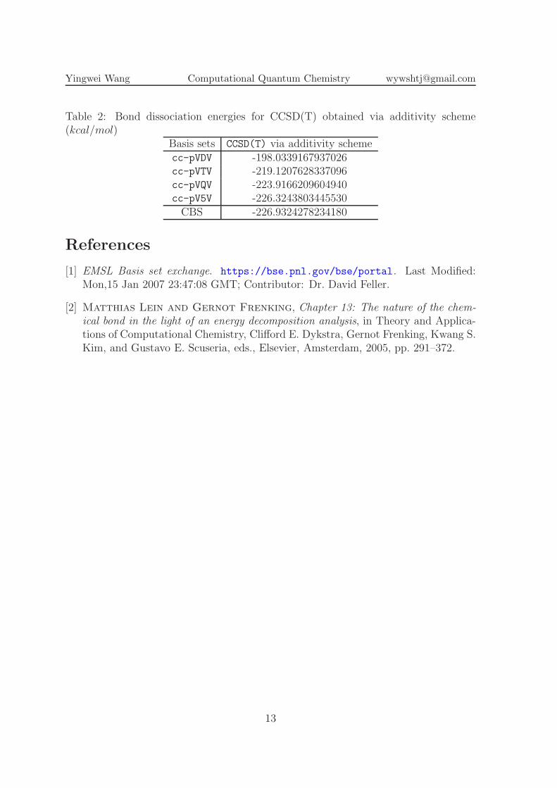
If the CCSD(T) energies for each basis set are computed via the formula (4.1), thenthe BDE values are shown in Table 2. We obverse that the CCSD(T) CBS BDE valueis a very good result compared to the experimental value given by (3.2).
4.6 Efficiency
Based on the results shown above, the computationally cheapest way to achievethe targeted accuracy (i.e., 1kcal/mol) in predicting BDE of N2 is that
1. first, calculating the energies by MP2;
2. second, obtaining CCSD(T) energies via additivity scheme (4.1);
3. third, computing the CBS values by extrapolation on HF energies and correlationenergies respectively;
4. fourth, getting the BDE from (3.1).
12
Yingwei Wang Computational Quantum Chemistry [email protected]
Table 2: Bond dissociation energies for CCSD(T) obtained via additivity scheme(kcal/mol)
Basis sets CCSD(T) via additivity schemecc-pVDV -198.0339167937026cc-pVTV -219.1207628337096cc-pVQV -223.9166209604940cc-pV5V -226.3243803445530CBS -226.9324278234180
References
[1] EMSL Basis set exchange. https://bse.pnl.gov/bse/portal. Last Modified:Mon,15 Jan 2007 23:47:08 GMT; Contributor: Dr. David Feller.
[2] Matthias Lein and Gernot Frenking, Chapter 13: The nature of the chem-
ical bond in the light of an energy decomposition analysis, in Theory and Applica-tions of Computational Chemistry, Clifford E. Dykstra, Gernot Frenking, Kwang S.Kim, and Gustavo E. Scuseria, eds., Elsevier, Amsterdam, 2005, pp. 291–372.
13
Yingwei Wang Computational Quantum Chemistry [email protected]
Purdue University
CHM 67300
Computational Quantum Chemistry
LAB REPOROT
Yingwei Wang
December 12, 2013
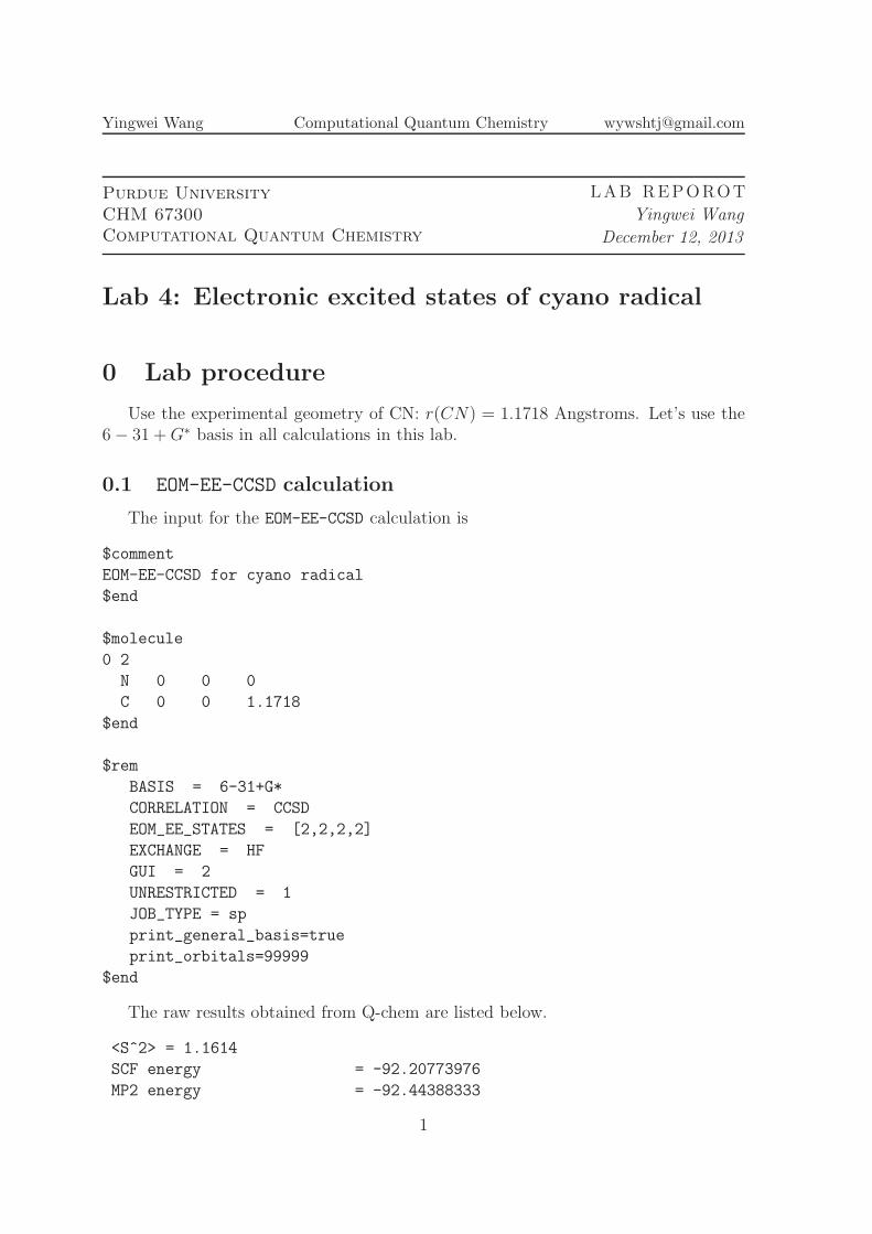
Lab 4: Electronic excited states of cyano radical
0 Lab procedure
Use the experimental geometry of CN: r(CN) = 1.1718 Angstroms. Let’s use the6− 31 +G∗ basis in all calculations in this lab.
0.1 EOM-EE-CCSD calculation
The input for the EOM-EE-CCSD calculation is
$comment
EOM-EE-CCSD for cyano radical
$end
$molecule
0 2
N 0 0 0
C 0 0 1.1718
$end
$rem
BASIS = 6-31+G*
CORRELATION = CCSD
EOM_EE_STATES = [2,2,2,2]
EXCHANGE = HF
GUI = 2
UNRESTRICTED = 1
JOB_TYPE = sp
print_general_basis=true
print_orbitals=99999
$end
The raw results obtained from Q-chem are listed below.
<S^2> = 1.1614
SCF energy = -92.20773976
MP2 energy = -92.44388333
1
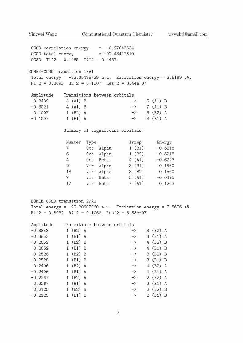
Yingwei Wang Computational Quantum Chemistry [email protected]
CCSD correlation energy = -0.27643634
CCSD total energy = -92.48417610
CCSD T1^2 = 0.1465 T2^2 = 0.1457.
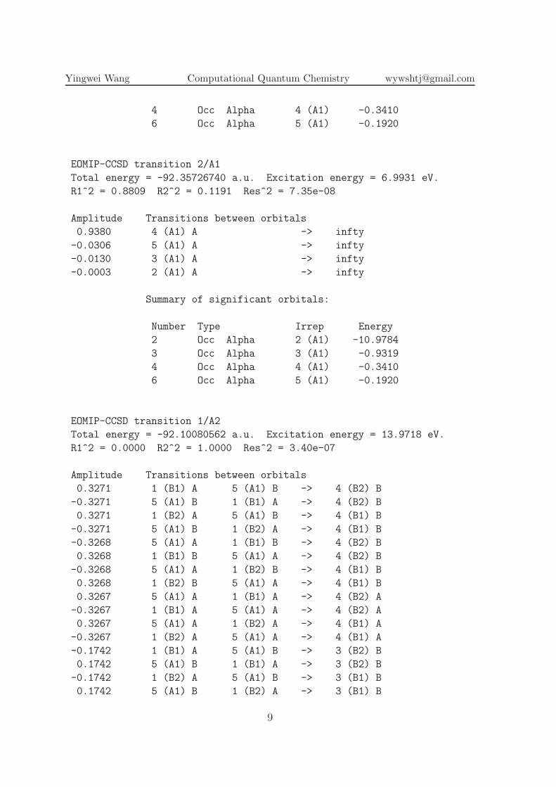
EOMEE-CCSD transition 1/A1
Total energy = -92.35485729 a.u. Excitation energy = 3.5189 eV.
R1^2 = 0.8693 R2^2 = 0.1307 Res^2 = 3.44e-07
Amplitude Transitions between orbitals
0.8439 4 (A1) B -> 5 (A1) B
-0.3021 4 (A1) B -> 7 (A1) B
0.1007 1 (B2) A -> 3 (B2) A
-0.1007 1 (B1) A -> 3 (B1) A
Summary of significant orbitals:
Number Type Irrep Energy
7 Occ Alpha 1 (B1) -0.5218
6 Occ Alpha 1 (B2) -0.5218
4 Occ Beta 4 (A1) -0.6223
21 Vir Alpha 3 (B1) 0.1560
18 Vir Alpha 3 (B2) 0.1560
7 Vir Beta 5 (A1) -0.0395
17 Vir Beta 7 (A1) 0.1263
EOMEE-CCSD transition 2/A1
Total energy = -92.20607060 a.u. Excitation energy = 7.5676 eV.
R1^2 = 0.8932 R2^2 = 0.1068 Res^2 = 6.58e-07
Amplitude Transitions between orbitals
-0.3853 1 (B2) A -> 3 (B2) A
-0.3853 1 (B1) A -> 3 (B1) A
-0.2659 1 (B2) B -> 4 (B2) B
0.2659 1 (B1) B -> 4 (B1) B
0.2528 1 (B2) B -> 3 (B2) B
-0.2528 1 (B1) B -> 3 (B1) B
0.2406 1 (B2) A -> 4 (B2) A
-0.2406 1 (B1) A -> 4 (B1) A
-0.2267 1 (B2) A -> 2 (B2) A
0.2267 1 (B1) A -> 2 (B1) A
0.2125 1 (B2) B -> 2 (B2) B
-0.2125 1 (B1) B -> 2 (B1) B
2
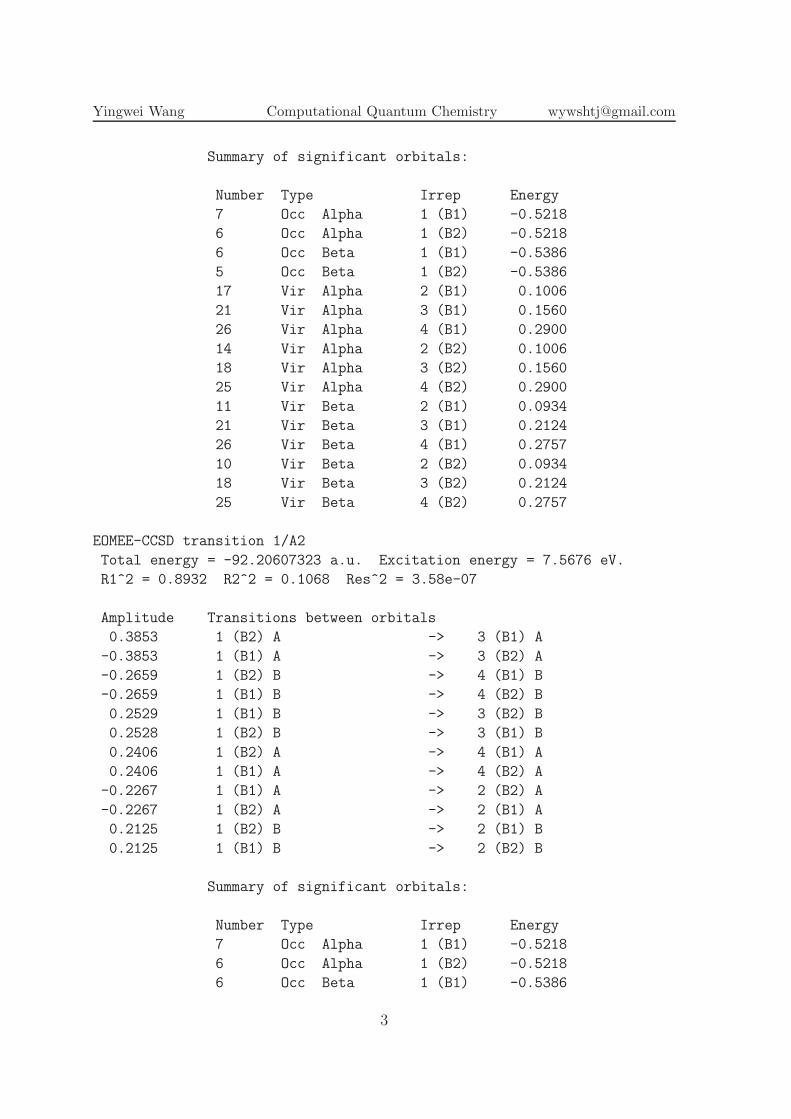
Yingwei Wang Computational Quantum Chemistry [email protected]
Summary of significant orbitals:
Number Type Irrep Energy
7 Occ Alpha 1 (B1) -0.5218
6 Occ Alpha 1 (B2) -0.5218
6 Occ Beta 1 (B1) -0.5386
5 Occ Beta 1 (B2) -0.5386
17 Vir Alpha 2 (B1) 0.1006
21 Vir Alpha 3 (B1) 0.1560
26 Vir Alpha 4 (B1) 0.2900
14 Vir Alpha 2 (B2) 0.1006
18 Vir Alpha 3 (B2) 0.1560
25 Vir Alpha 4 (B2) 0.2900
11 Vir Beta 2 (B1) 0.0934
21 Vir Beta 3 (B1) 0.2124
26 Vir Beta 4 (B1) 0.2757
10 Vir Beta 2 (B2) 0.0934
18 Vir Beta 3 (B2) 0.2124
25 Vir Beta 4 (B2) 0.2757
EOMEE-CCSD transition 1/A2
Total energy = -92.20607323 a.u. Excitation energy = 7.5676 eV.
R1^2 = 0.8932 R2^2 = 0.1068 Res^2 = 3.58e-07
Amplitude Transitions between orbitals
0.3853 1 (B2) A -> 3 (B1) A
-0.3853 1 (B1) A -> 3 (B2) A
-0.2659 1 (B2) B -> 4 (B1) B
-0.2659 1 (B1) B -> 4 (B2) B
0.2529 1 (B1) B -> 3 (B2) B
0.2528 1 (B2) B -> 3 (B1) B
0.2406 1 (B2) A -> 4 (B1) A
0.2406 1 (B1) A -> 4 (B2) A
-0.2267 1 (B1) A -> 2 (B2) A
-0.2267 1 (B2) A -> 2 (B1) A
0.2125 1 (B2) B -> 2 (B1) B
0.2125 1 (B1) B -> 2 (B2) B
Summary of significant orbitals:
Number Type Irrep Energy
7 Occ Alpha 1 (B1) -0.5218
6 Occ Alpha 1 (B2) -0.5218
6 Occ Beta 1 (B1) -0.5386
3
Yingwei Wang Computational Quantum Chemistry [email protected]
5 Occ Beta 1 (B2) -0.5386
17 Vir Alpha 2 (B1) 0.1006
21 Vir Alpha 3 (B1) 0.1560
26 Vir Alpha 4 (B1) 0.2900
14 Vir Alpha 2 (B2) 0.1006
18 Vir Alpha 3 (B2) 0.1560
25 Vir Alpha 4 (B2) 0.2900
11 Vir Beta 2 (B1) 0.0934
21 Vir Beta 3 (B1) 0.2124
26 Vir Beta 4 (B1) 0.2757
10 Vir Beta 2 (B2) 0.0934
18 Vir Beta 3 (B2) 0.2124
25 Vir Beta 4 (B2) 0.2757
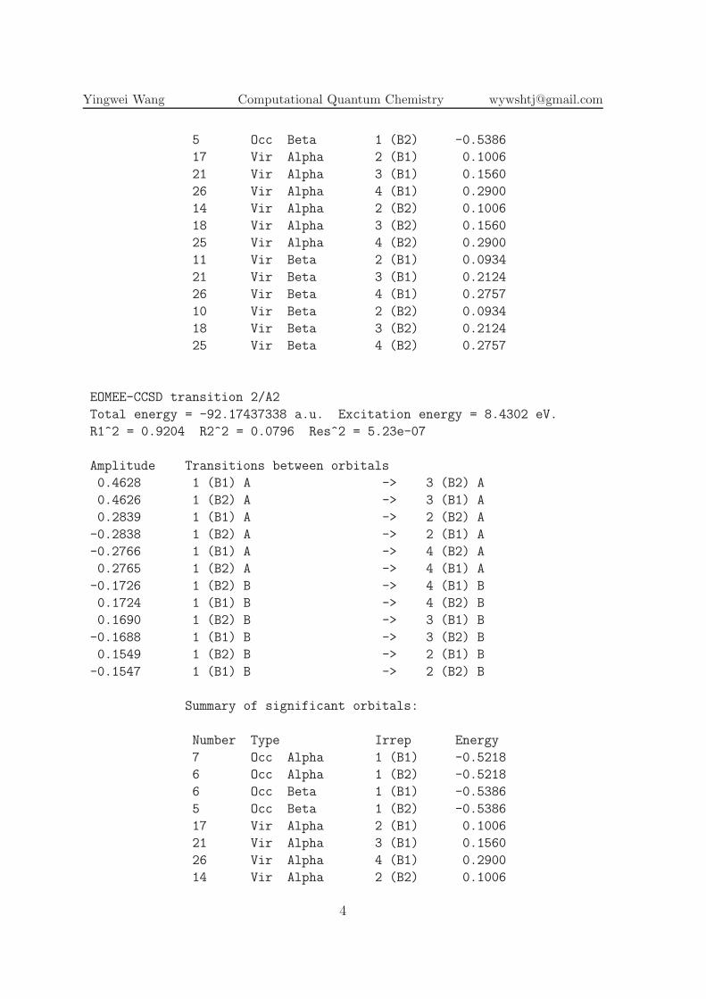
EOMEE-CCSD transition 2/A2
Total energy = -92.17437338 a.u. Excitation energy = 8.4302 eV.
R1^2 = 0.9204 R2^2 = 0.0796 Res^2 = 5.23e-07
Amplitude Transitions between orbitals
0.4628 1 (B1) A -> 3 (B2) A
0.4626 1 (B2) A -> 3 (B1) A
0.2839 1 (B1) A -> 2 (B2) A
-0.2838 1 (B2) A -> 2 (B1) A
-0.2766 1 (B1) A -> 4 (B2) A
0.2765 1 (B2) A -> 4 (B1) A
-0.1726 1 (B2) B -> 4 (B1) B
0.1724 1 (B1) B -> 4 (B2) B
0.1690 1 (B2) B -> 3 (B1) B
-0.1688 1 (B1) B -> 3 (B2) B
0.1549 1 (B2) B -> 2 (B1) B
-0.1547 1 (B1) B -> 2 (B2) B
Summary of significant orbitals:
Number Type Irrep Energy
7 Occ Alpha 1 (B1) -0.5218
6 Occ Alpha 1 (B2) -0.5218
6 Occ Beta 1 (B1) -0.5386
5 Occ Beta 1 (B2) -0.5386
17 Vir Alpha 2 (B1) 0.1006
21 Vir Alpha 3 (B1) 0.1560
26 Vir Alpha 4 (B1) 0.2900
14 Vir Alpha 2 (B2) 0.1006
4
Yingwei Wang Computational Quantum Chemistry [email protected]
18 Vir Alpha 3 (B2) 0.1560
25 Vir Alpha 4 (B2) 0.2900
11 Vir Beta 2 (B1) 0.0934
21 Vir Beta 3 (B1) 0.2124
26 Vir Beta 4 (B1) 0.2757
10 Vir Beta 2 (B2) 0.0934
18 Vir Beta 3 (B2) 0.2124
25 Vir Beta 4 (B2) 0.2757
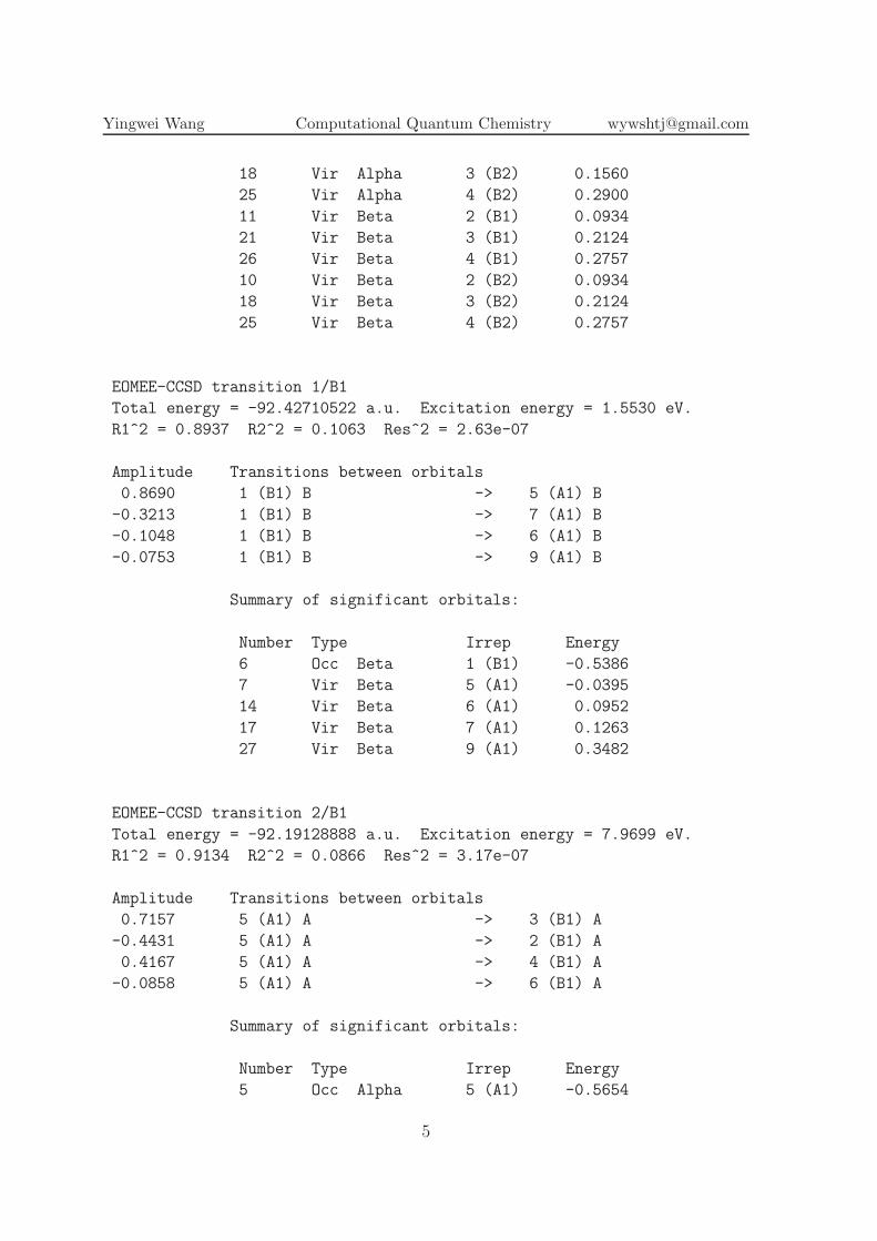
EOMEE-CCSD transition 1/B1
Total energy = -92.42710522 a.u. Excitation energy = 1.5530 eV.
R1^2 = 0.8937 R2^2 = 0.1063 Res^2 = 2.63e-07
Amplitude Transitions between orbitals
0.8690 1 (B1) B -> 5 (A1) B
-0.3213 1 (B1) B -> 7 (A1) B
-0.1048 1 (B1) B -> 6 (A1) B
-0.0753 1 (B1) B -> 9 (A1) B
Summary of significant orbitals:
Number Type Irrep Energy
6 Occ Beta 1 (B1) -0.5386
7 Vir Beta 5 (A1) -0.0395
14 Vir Beta 6 (A1) 0.0952
17 Vir Beta 7 (A1) 0.1263
27 Vir Beta 9 (A1) 0.3482
EOMEE-CCSD transition 2/B1
Total energy = -92.19128888 a.u. Excitation energy = 7.9699 eV.
R1^2 = 0.9134 R2^2 = 0.0866 Res^2 = 3.17e-07
Amplitude Transitions between orbitals
0.7157 5 (A1) A -> 3 (B1) A
-0.4431 5 (A1) A -> 2 (B1) A
0.4167 5 (A1) A -> 4 (B1) A
-0.0858 5 (A1) A -> 6 (B1) A
Summary of significant orbitals:
Number Type Irrep Energy
5 Occ Alpha 5 (A1) -0.5654
5
Yingwei Wang Computational Quantum Chemistry [email protected]
17 Vir Alpha 2 (B1) 0.1006
21 Vir Alpha 3 (B1) 0.1560
26 Vir Alpha 4 (B1) 0.2900
32 Vir Alpha 6 (B1) 1.2184
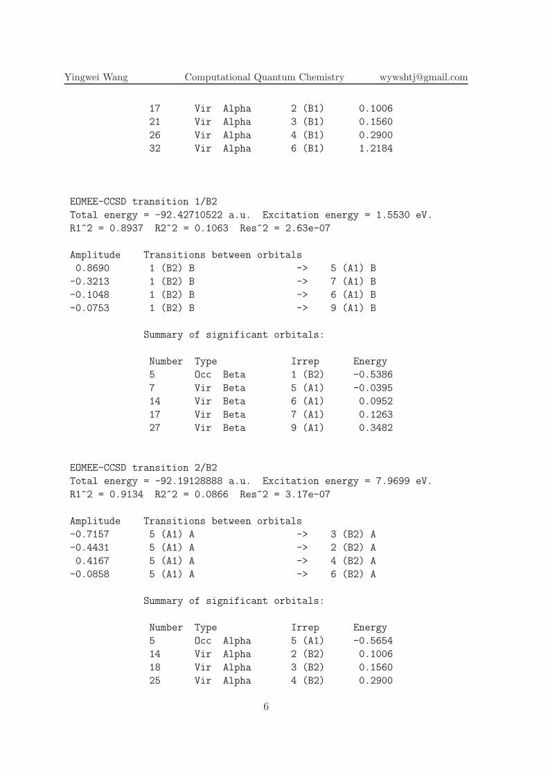
EOMEE-CCSD transition 1/B2
Total energy = -92.42710522 a.u. Excitation energy = 1.5530 eV.
R1^2 = 0.8937 R2^2 = 0.1063 Res^2 = 2.63e-07
Amplitude Transitions between orbitals
0.8690 1 (B2) B -> 5 (A1) B
-0.3213 1 (B2) B -> 7 (A1) B
-0.1048 1 (B2) B -> 6 (A1) B
-0.0753 1 (B2) B -> 9 (A1) B
Summary of significant orbitals:
Number Type Irrep Energy
5 Occ Beta 1 (B2) -0.5386
7 Vir Beta 5 (A1) -0.0395
14 Vir Beta 6 (A1) 0.0952
17 Vir Beta 7 (A1) 0.1263
27 Vir Beta 9 (A1) 0.3482
EOMEE-CCSD transition 2/B2
Total energy = -92.19128888 a.u. Excitation energy = 7.9699 eV.
R1^2 = 0.9134 R2^2 = 0.0866 Res^2 = 3.17e-07
Amplitude Transitions between orbitals
-0.7157 5 (A1) A -> 3 (B2) A
-0.4431 5 (A1) A -> 2 (B2) A
0.4167 5 (A1) A -> 4 (B2) A
-0.0858 5 (A1) A -> 6 (B2) A
Summary of significant orbitals:
Number Type Irrep Energy
5 Occ Alpha 5 (A1) -0.5654
14 Vir Alpha 2 (B2) 0.1006
18 Vir Alpha 3 (B2) 0.1560
25 Vir Alpha 4 (B2) 0.2900
6
Yingwei Wang Computational Quantum Chemistry [email protected]
28 Vir Alpha 6 (B2) 1.2184
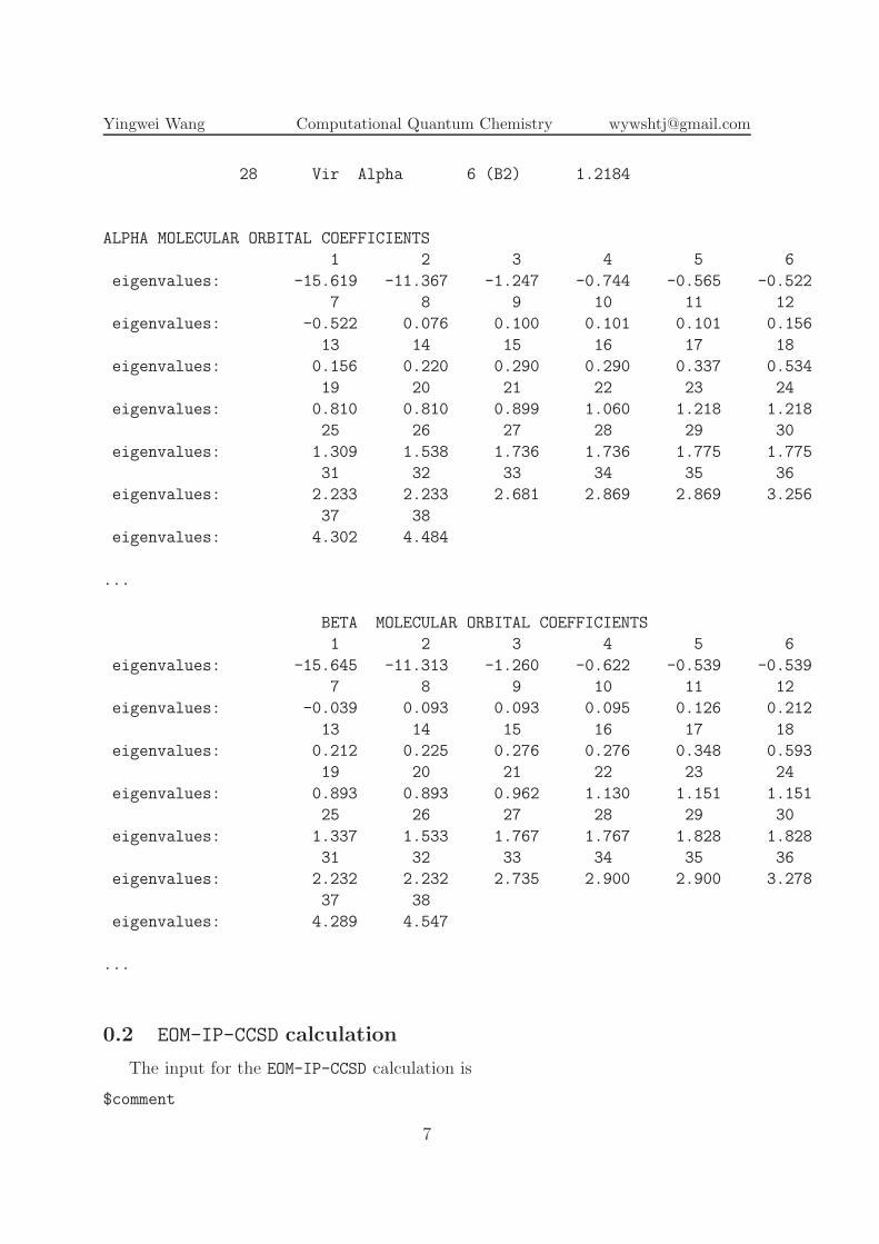
ALPHA MOLECULAR ORBITAL COEFFICIENTS
1 2 3 4 5 6
eigenvalues: -15.619 -11.367 -1.247 -0.744 -0.565 -0.522
7 8 9 10 11 12
eigenvalues: -0.522 0.076 0.100 0.101 0.101 0.156
13 14 15 16 17 18
eigenvalues: 0.156 0.220 0.290 0.290 0.337 0.534
19 20 21 22 23 24
eigenvalues: 0.810 0.810 0.899 1.060 1.218 1.218
25 26 27 28 29 30
eigenvalues: 1.309 1.538 1.736 1.736 1.775 1.775
31 32 33 34 35 36
eigenvalues: 2.233 2.233 2.681 2.869 2.869 3.256
37 38
eigenvalues: 4.302 4.484
...
BETA MOLECULAR ORBITAL COEFFICIENTS
1 2 3 4 5 6
eigenvalues: -15.645 -11.313 -1.260 -0.622 -0.539 -0.539
7 8 9 10 11 12
eigenvalues: -0.039 0.093 0.093 0.095 0.126 0.212
13 14 15 16 17 18
eigenvalues: 0.212 0.225 0.276 0.276 0.348 0.593
19 20 21 22 23 24
eigenvalues: 0.893 0.893 0.962 1.130 1.151 1.151
25 26 27 28 29 30
eigenvalues: 1.337 1.533 1.767 1.767 1.828 1.828
31 32 33 34 35 36
eigenvalues: 2.232 2.232 2.735 2.900 2.900 3.278
37 38
eigenvalues: 4.289 4.547
...
0.2 EOM-IP-CCSD calculation
The input for the EOM-IP-CCSD calculation is
$comment
7
Yingwei Wang Computational Quantum Chemistry [email protected]
EOM-IP-CCSD for cyano radical
$end
$molecule
-1 1
N 0 0 0
C 0 0 1.1718
$end
$rem
BASIS = 6-31+G*
CORRELATION = CCSD
EOM_IP_STATES = [2,2,2,2]
EXCHANGE = HF
GUI = 2
UNRESTRICTED = 1
JOB_TYPE = sp
print_general_basis=true
print_orbitals=99999
$end
The raw results obtained from Q-chem are listed below.
<S^2> = 0.0000
SCF energy = -92.31462822
MP2 energy = -92.60987126
CCSD correlation energy = -0.29963068
CCSD total energy = -92.61425890
CCSD T1^2 = 0.0080 T2^2 = 0.1235.
EOMIP-CCSD transition 1/A1
Total energy = -92.47751457 a.u. Excitation energy = 3.7210 eV.
R1^2 = 0.9158 R2^2 = 0.0842 Res^2 = 9.73e-08
Amplitude Transitions between orbitals
-0.9561 5 (A1) A -> infty
-0.0386 4 (A1) A -> infty
0.0135 3 (A1) A -> infty
-0.0003 2 (A1) A -> infty
Summary of significant orbitals:
Number Type Irrep Energy
2 Occ Alpha 2 (A1) -10.9784
3 Occ Alpha 3 (A1) -0.9319
8
Yingwei Wang Computational Quantum Chemistry [email protected]
4 Occ Alpha 4 (A1) -0.3410
6 Occ Alpha 5 (A1) -0.1920
EOMIP-CCSD transition 2/A1
Total energy = -92.35726740 a.u. Excitation energy = 6.9931 eV.
R1^2 = 0.8809 R2^2 = 0.1191 Res^2 = 7.35e-08
Amplitude Transitions between orbitals
0.9380 4 (A1) A -> infty
-0.0306 5 (A1) A -> infty
-0.0130 3 (A1) A -> infty
-0.0003 2 (A1) A -> infty
Summary of significant orbitals:
Number Type Irrep Energy
2 Occ Alpha 2 (A1) -10.9784
3 Occ Alpha 3 (A1) -0.9319
4 Occ Alpha 4 (A1) -0.3410
6 Occ Alpha 5 (A1) -0.1920
EOMIP-CCSD transition 1/A2
Total energy = -92.10080562 a.u. Excitation energy = 13.9718 eV.
R1^2 = 0.0000 R2^2 = 1.0000 Res^2 = 3.40e-07
Amplitude Transitions between orbitals
0.3271 1 (B1) A 5 (A1) B -> 4 (B2) B
-0.3271 5 (A1) B 1 (B1) A -> 4 (B2) B
0.3271 1 (B2) A 5 (A1) B -> 4 (B1) B
-0.3271 5 (A1) B 1 (B2) A -> 4 (B1) B
-0.3268 5 (A1) A 1 (B1) B -> 4 (B2) B
0.3268 1 (B1) B 5 (A1) A -> 4 (B2) B
-0.3268 5 (A1) A 1 (B2) B -> 4 (B1) B
0.3268 1 (B2) B 5 (A1) A -> 4 (B1) B
0.3267 5 (A1) A 1 (B1) A -> 4 (B2) A
-0.3267 1 (B1) A 5 (A1) A -> 4 (B2) A
0.3267 5 (A1) A 1 (B2) A -> 4 (B1) A
-0.3267 1 (B2) A 5 (A1) A -> 4 (B1) A
-0.1742 1 (B1) A 5 (A1) B -> 3 (B2) B
0.1742 5 (A1) B 1 (B1) A -> 3 (B2) B
-0.1742 1 (B2) A 5 (A1) B -> 3 (B1) B
0.1742 5 (A1) B 1 (B2) A -> 3 (B1) B
9
Yingwei Wang Computational Quantum Chemistry [email protected]
0.1740 5 (A1) A 1 (B1) B -> 3 (B2) B
-0.1740 1 (B1) B 5 (A1) A -> 3 (B2) B
0.1740 5 (A1) A 1 (B2) B -> 3 (B1) B
-0.1740 1 (B2) B 5 (A1) A -> 3 (B1) B
-0.1740 5 (A1) A 1 (B1) A -> 3 (B2) A
0.1740 1 (B1) A 5 (A1) A -> 3 (B2) A
-0.1740 5 (A1) A 1 (B2) A -> 3 (B1) A
0.1740 1 (B2) A 5 (A1) A -> 3 (B1) A
-0.1089 1 (B1) A 5 (A1) B -> 2 (B2) B
0.1089 5 (A1) B 1 (B1) A -> 2 (B2) B
-0.1089 1 (B2) A 5 (A1) B -> 2 (B1) B
0.1089 5 (A1) B 1 (B2) A -> 2 (B1) B
0.1087 5 (A1) A 1 (B1) B -> 2 (B2) B
-0.1087 1 (B1) B 5 (A1) A -> 2 (B2) B
0.1087 5 (A1) A 1 (B2) B -> 2 (B1) B
-0.1087 1 (B2) B 5 (A1) A -> 2 (B1) B
-0.1087 5 (A1) A 1 (B1) A -> 2 (B2) A
0.1087 1 (B1) A 5 (A1) A -> 2 (B2) A
-0.1087 5 (A1) A 1 (B2) A -> 2 (B1) A
0.1087 1 (B2) A 5 (A1) A -> 2 (B1) A
Summary of significant orbitals:
Number Type Irrep Energy
6 Occ Alpha 5 (A1) -0.1920
5 Occ Alpha 1 (B1) -0.1947
7 Occ Alpha 1 (B2) -0.1947
6 Occ Beta 5 (A1) -0.1920
5 Occ Beta 1 (B1) -0.1947
7 Occ Beta 1 (B2) -0.1947
12 Vir Alpha 2 (B1) 0.2754
22 Vir Alpha 3 (B1) 0.4071
26 Vir Alpha 4 (B1) 0.5312
11 Vir Alpha 2 (B2) 0.2754
21 Vir Alpha 3 (B2) 0.4071
25 Vir Alpha 4 (B2) 0.5312
12 Vir Beta 2 (B1) 0.2754
22 Vir Beta 3 (B1) 0.4071
26 Vir Beta 4 (B1) 0.5312
11 Vir Beta 2 (B2) 0.2754
21 Vir Beta 3 (B2) 0.4071
25 Vir Beta 4 (B2) 0.5312
10
Yingwei Wang Computational Quantum Chemistry [email protected]
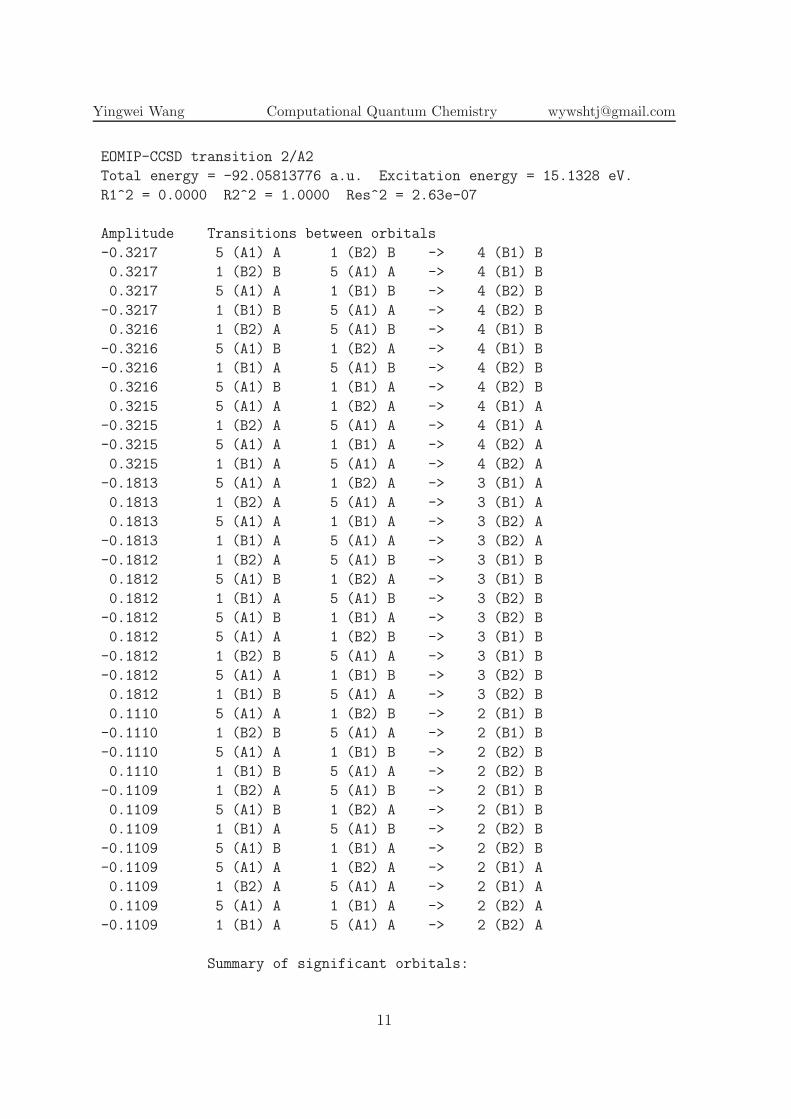
EOMIP-CCSD transition 2/A2
Total energy = -92.05813776 a.u. Excitation energy = 15.1328 eV.
R1^2 = 0.0000 R2^2 = 1.0000 Res^2 = 2.63e-07
Amplitude Transitions between orbitals
-0.3217 5 (A1) A 1 (B2) B -> 4 (B1) B
0.3217 1 (B2) B 5 (A1) A -> 4 (B1) B
0.3217 5 (A1) A 1 (B1) B -> 4 (B2) B
-0.3217 1 (B1) B 5 (A1) A -> 4 (B2) B
0.3216 1 (B2) A 5 (A1) B -> 4 (B1) B
-0.3216 5 (A1) B 1 (B2) A -> 4 (B1) B
-0.3216 1 (B1) A 5 (A1) B -> 4 (B2) B
0.3216 5 (A1) B 1 (B1) A -> 4 (B2) B
0.3215 5 (A1) A 1 (B2) A -> 4 (B1) A
-0.3215 1 (B2) A 5 (A1) A -> 4 (B1) A
-0.3215 5 (A1) A 1 (B1) A -> 4 (B2) A
0.3215 1 (B1) A 5 (A1) A -> 4 (B2) A
-0.1813 5 (A1) A 1 (B2) A -> 3 (B1) A
0.1813 1 (B2) A 5 (A1) A -> 3 (B1) A
0.1813 5 (A1) A 1 (B1) A -> 3 (B2) A
-0.1813 1 (B1) A 5 (A1) A -> 3 (B2) A
-0.1812 1 (B2) A 5 (A1) B -> 3 (B1) B
0.1812 5 (A1) B 1 (B2) A -> 3 (B1) B
0.1812 1 (B1) A 5 (A1) B -> 3 (B2) B
-0.1812 5 (A1) B 1 (B1) A -> 3 (B2) B
0.1812 5 (A1) A 1 (B2) B -> 3 (B1) B
-0.1812 1 (B2) B 5 (A1) A -> 3 (B1) B
-0.1812 5 (A1) A 1 (B1) B -> 3 (B2) B
0.1812 1 (B1) B 5 (A1) A -> 3 (B2) B
0.1110 5 (A1) A 1 (B2) B -> 2 (B1) B
-0.1110 1 (B2) B 5 (A1) A -> 2 (B1) B
-0.1110 5 (A1) A 1 (B1) B -> 2 (B2) B
0.1110 1 (B1) B 5 (A1) A -> 2 (B2) B
-0.1109 1 (B2) A 5 (A1) B -> 2 (B1) B
0.1109 5 (A1) B 1 (B2) A -> 2 (B1) B
0.1109 1 (B1) A 5 (A1) B -> 2 (B2) B
-0.1109 5 (A1) B 1 (B1) A -> 2 (B2) B
-0.1109 5 (A1) A 1 (B2) A -> 2 (B1) A
0.1109 1 (B2) A 5 (A1) A -> 2 (B1) A
0.1109 5 (A1) A 1 (B1) A -> 2 (B2) A
-0.1109 1 (B1) A 5 (A1) A -> 2 (B2) A
Summary of significant orbitals:
11
Yingwei Wang Computational Quantum Chemistry [email protected]
Number Type Irrep Energy
6 Occ Alpha 5 (A1) -0.1920
5 Occ Alpha 1 (B1) -0.1947
7 Occ Alpha 1 (B2) -0.1947
6 Occ Beta 5 (A1) -0.1920
5 Occ Beta 1 (B1) -0.1947
7 Occ Beta 1 (B2) -0.1947
12 Vir Alpha 2 (B1) 0.2754
22 Vir Alpha 3 (B1) 0.4071
26 Vir Alpha 4 (B1) 0.5312
11 Vir Alpha 2 (B2) 0.2754
21 Vir Alpha 3 (B2) 0.4071
25 Vir Alpha 4 (B2) 0.5312
12 Vir Beta 2 (B1) 0.2754
22 Vir Beta 3 (B1) 0.4071
26 Vir Beta 4 (B1) 0.5312
11 Vir Beta 2 (B2) 0.2754
21 Vir Beta 3 (B2) 0.4071
25 Vir Beta 4 (B2) 0.5312
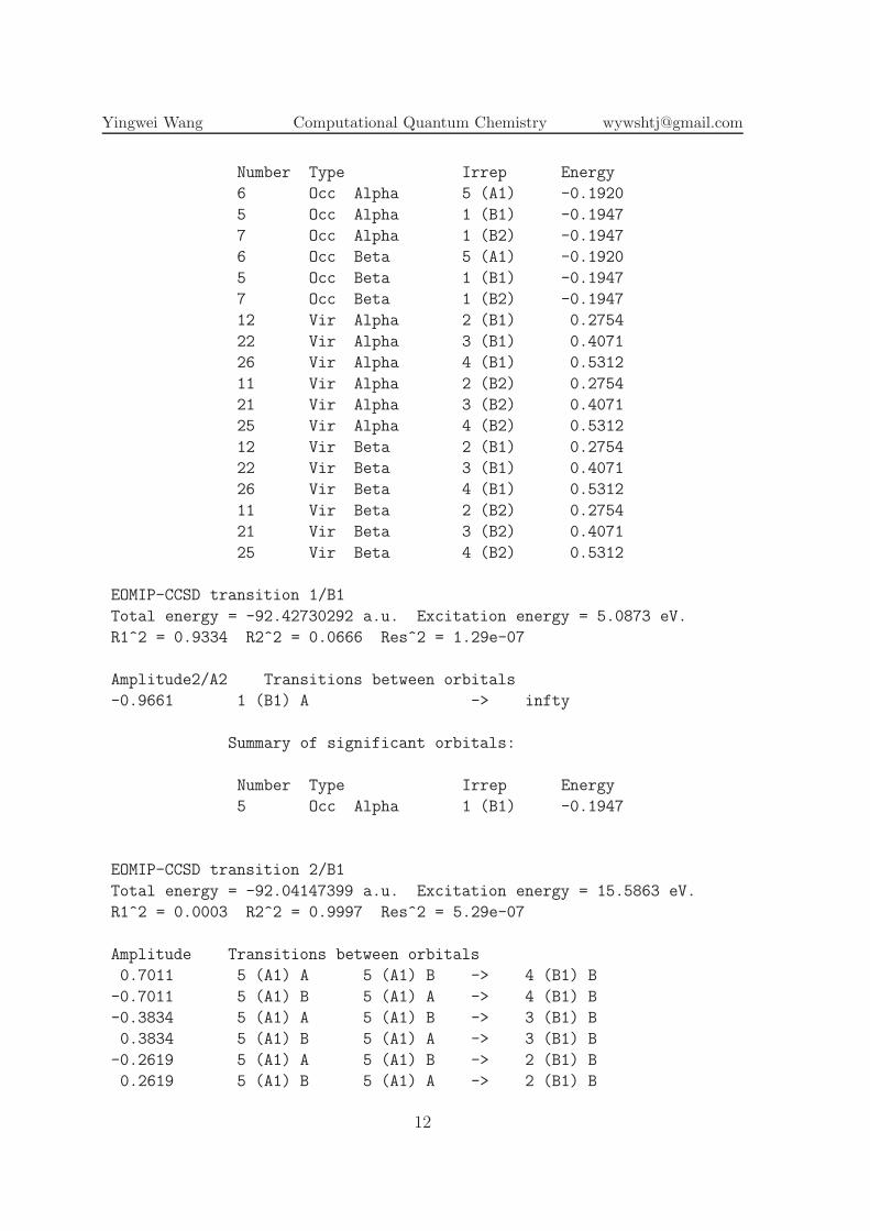
EOMIP-CCSD transition 1/B1
Total energy = -92.42730292 a.u. Excitation energy = 5.0873 eV.
R1^2 = 0.9334 R2^2 = 0.0666 Res^2 = 1.29e-07
Amplitude2/A2 Transitions between orbitals
-0.9661 1 (B1) A -> infty
Summary of significant orbitals:
Number Type Irrep Energy
5 Occ Alpha 1 (B1) -0.1947
EOMIP-CCSD transition 2/B1
Total energy = -92.04147399 a.u. Excitation energy = 15.5863 eV.
R1^2 = 0.0003 R2^2 = 0.9997 Res^2 = 5.29e-07
Amplitude Transitions between orbitals
0.7011 5 (A1) A 5 (A1) B -> 4 (B1) B
-0.7011 5 (A1) B 5 (A1) A -> 4 (B1) B
-0.3834 5 (A1) A 5 (A1) B -> 3 (B1) B
0.3834 5 (A1) B 5 (A1) A -> 3 (B1) B
-0.2619 5 (A1) A 5 (A1) B -> 2 (B1) B
0.2619 5 (A1) B 5 (A1) A -> 2 (B1) B
12
Yingwei Wang Computational Quantum Chemistry [email protected]
0.2585 5 (A1) A 4 (A1) B -> 4 (B1) B
-0.2585 4 (A1) B 5 (A1) A -> 4 (B1) B
-0.2543 4 (A1) A 4 (A1) B -> 4 (B1) B
0.2543 4 (A1) B 4 (A1) A -> 4 (B1) B
0.1790 4 (A1) A 5 (A1) B -> 4 (B1) B
-0.1790 5 (A1) B 4 (A1) A -> 4 (B1) B
-0.1566 5 (A1) A 5 (A1) B -> 5 (B1) B
0.1566 5 (A1) B 5 (A1) A -> 5 (B1) B
0.1374 4 (A1) A 4 (A1) B -> 3 (B1) B
-0.1374 4 (A1) B 4 (A1) A -> 3 (B1) B
-0.1268 5 (A1) A 4 (A1) B -> 3 (B1) B
0.1268 4 (A1) B 5 (A1) A -> 3 (B1) B
-0.1046 5 (A1) A 4 (A1) B -> 2 (B1) B
0.1046 4 (A1) B 5 (A1) A -> 2 (B1) B
0.1016 4 (A1) A 4 (A1) B -> 2 (B1) B
-0.1016 4 (A1) B 4 (A1) A -> 2 (B1) B
Summary of significant orbitals:
Number Type Irrep Energy
4 Occ Alpha 4 (A1) -0.3410
6 Occ Alpha 5 (A1) -0.1920
4 Occ Beta 4 (A1) -0.3410
6 Occ Beta 5 (A1) -0.1920
12 Vir Beta 2 (B1) 0.2754
22 Vir Beta 3 (B1) 0.4071
26 Vir Beta 4 (B1) 0.5312
36 Vir Beta 5 (B1) 1.1622
EOMIP-CCSD transition 1/B2
Total energy = -92.42730292 a.u. Excitation energy = 5.0873 eV.
R1^2 = 0.9334 R2^2 = 0.0666 Res^2 = 1.29e-07
Amplitude Transitions between orbitals
-0.9661 1 (B2) A -> infty
Summary of significant orbitals:
Number Type Irrep Energy
7 Occ Alpha 1 (B2) -0.1947
EOMIP-CCSD transition 2/B2
Total energy = -92.04147468 a.u. Excitation energy = 15.5863 eV.
13
Yingwei Wang Computational Quantum Chemistry [email protected]
R1^2 = 0.0003 R2^2 = 0.9997 Res^2 = 5.39e-07
Amplitude Transitions between orbitals
0.7011 5 (A1) A 5 (A1) B -> 4 (B2) B
-0.7011 5 (A1) B 5 (A1) A -> 4 (B2) B
-0.3834 5 (A1) A 5 (A1) B -> 3 (B2) B
0.3834 5 (A1) B 5 (A1) A -> 3 (B2) B
-0.2619 5 (A1) A 5 (A1) B -> 2 (B2) B
0.2619 5 (A1) B 5 (A1) A -> 2 (B2) B
0.2584 5 (A1) A 4 (A1) B -> 4 (B2) B
-0.2584 4 (A1) B 5 (A1) A -> 4 (B2) B
-0.2543 4 (A1) A 4 (A1) B -> 4 (B2) B
0.2543 4 (A1) B 4 (A1) A -> 4 (B2) B
0.1791 4 (A1) A 5 (A1) B -> 4 (B2) B
-0.1791 5 (A1) B 4 (A1) A -> 4 (B2) B
0.1566 5 (A1) A 5 (A1) B -> 5 (B2) B
-0.1566 5 (A1) B 5 (A1) A -> 5 (B2) B
0.1374 4 (A1) A 4 (A1) B -> 3 (B2) B
-0.1374 4 (A1) B 4 (A1) A -> 3 (B2) B
-0.1267 5 (A1) A 4 (A1) B -> 3 (B2) B
0.1267 4 (A1) B 5 (A1) A -> 3 (B2) B
-0.1045 5 (A1) A 4 (A1) B -> 2 (B2) B
0.1045 4 (A1) B 5 (A1) A -> 2 (B2) B
0.1016 4 (A1) A 4 (A1) B -> 2 (B2) B
-0.1016 4 (A1) B 4 (A1) A -> 2 (B2) B
Summary of significant orbitals:
Number Type Irrep Energy
4 Occ Alpha 4 (A1) -0.3410
6 Occ Alpha 5 (A1) -0.1920
4 Occ Beta 4 (A1) -0.3410
6 Occ Beta 5 (A1) -0.1920
11 Vir Beta 2 (B2) 0.2754
21 Vir Beta 3 (B2) 0.4071
25 Vir Beta 4 (B2) 0.5312
33 Vir Beta 5 (B2) 1.1622
ALPHA MOLECULAR ORBITAL COEFFICIENTS
ALPHA MOLECULAR ORBITAL COEFFICIENTS
1 2 3 4 5 6
eigenvalues: -15.301 -10.978 -0.932 -0.341 -0.195 -0.195
14
Yingwei Wang Computational Quantum Chemistry [email protected]
7 8 9 10 11 12
eigenvalues: -0.192 0.248 0.275 0.275 0.289 0.405
13 14 15 16 17 18
eigenvalues: 0.407 0.407 0.531 0.531 0.553 0.850
19 20 21 22 23 24
eigenvalues: 1.162 1.162 1.224 1.383 1.461 1.461
25 26 27 28 29 30
eigenvalues: 1.618 1.818 2.084 2.084 2.136 2.136
31 32 33 34 35 36
eigenvalues: 2.551 2.551 3.045 3.217 3.217 3.592
37 38
eigenvalues: 4.599 4.866
...
BETA MOLECULAR ORBITAL COEFFICIENTS
1 2 3 4 5 6
eigenvalues: -15.301 -10.978 -0.932 -0.341 -0.195 -0.195
7 8 9 10 11 12
eigenvalues: -0.192 0.248 0.275 0.275 0.289 0.405
13 14 15 16 17 18
eigenvalues: 0.407 0.407 0.531 0.531 0.553 0.850
19 20 21 22 23 24
eigenvalues: 1.162 1.162 1.224 1.383 1.461 1.461
25 26 27 28 29 30
eigenvalues: 1.618 1.818 2.084 2.084 2.136 2.136
31 32 33 34 35 36
eigenvalues: 2.551 2.551 3.045 3.217 3.217 3.592
37 38
eigenvalues: 4.599 4.866
...
15
Yingwei Wang Computational Quantum Chemistry [email protected]
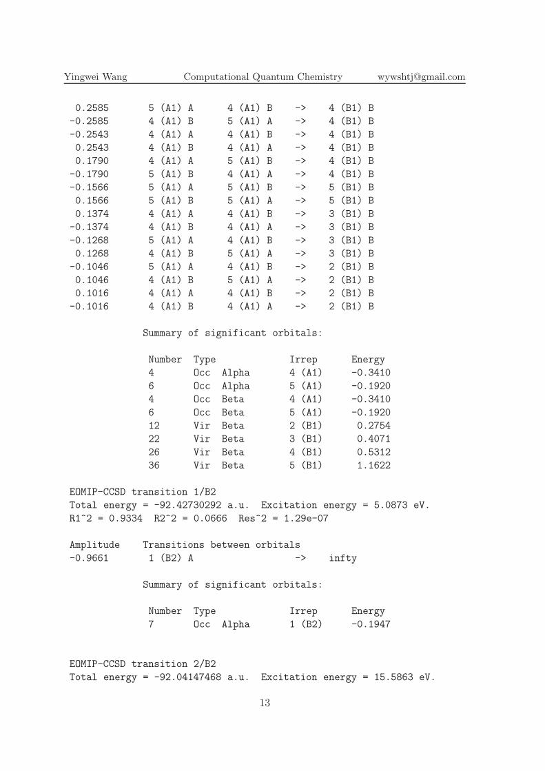
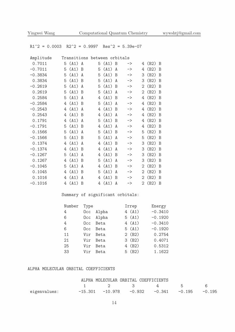
1 MO
Draw molecular orbitals of CN.
Figure 1: Molecular orbital from EOM-EE-CCSD
Figure 2: Molecular orbital from EOM-IP-CCSD
16

Yingwei Wang Computational Quantum Chemistry [email protected]
2 Analyze EOM-EE-CCSD output
Figure 3: Surface: Alpha 1 (EOM-EE-CCSD)
Figure 4: Surface: Alpha 2 (EOM-EE-CCSD)
17
Yingwei Wang Computational Quantum Chemistry [email protected]
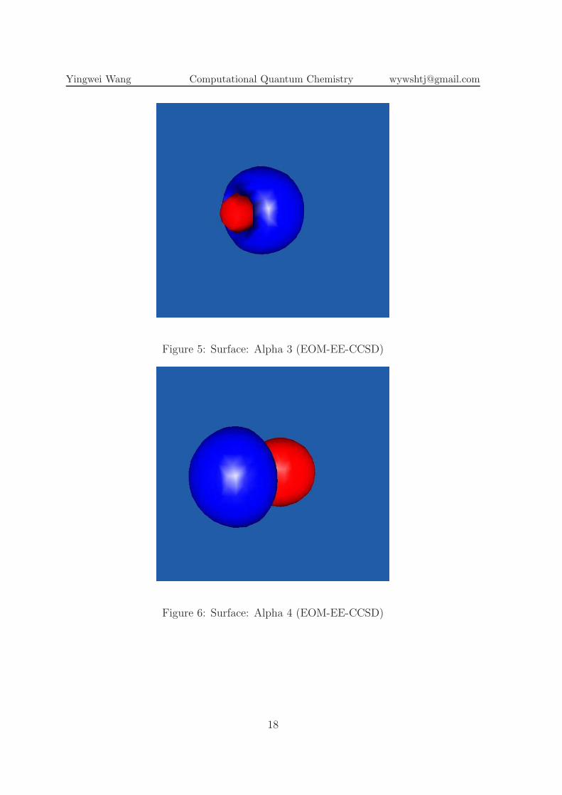
Figure 5: Surface: Alpha 3 (EOM-EE-CCSD)
Figure 6: Surface: Alpha 4 (EOM-EE-CCSD)
18
Yingwei Wang Computational Quantum Chemistry [email protected]
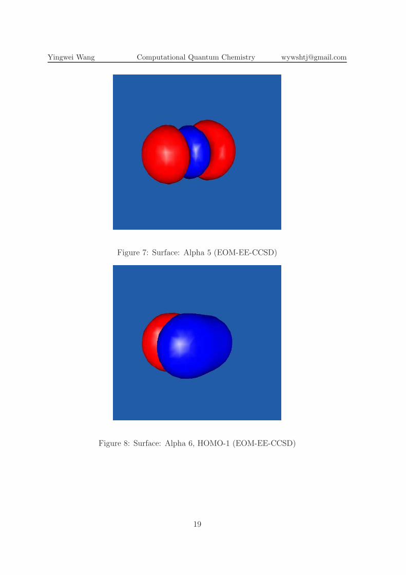
Figure 7: Surface: Alpha 5 (EOM-EE-CCSD)
Figure 8: Surface: Alpha 6, HOMO-1 (EOM-EE-CCSD)
19
Yingwei Wang Computational Quantum Chemistry [email protected]
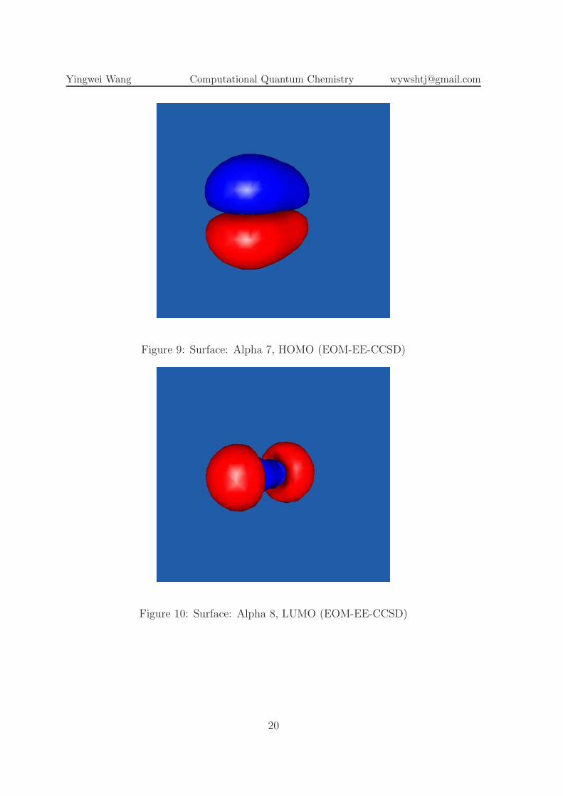
Figure 9: Surface: Alpha 7, HOMO (EOM-EE-CCSD)
Figure 10: Surface: Alpha 8, LUMO (EOM-EE-CCSD)
20
Yingwei Wang Computational Quantum Chemistry [email protected]
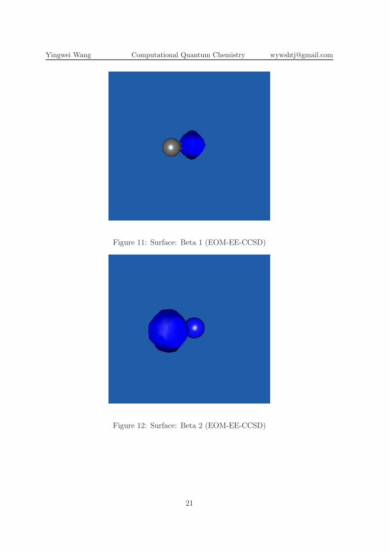
Figure 11: Surface: Beta 1 (EOM-EE-CCSD)
Figure 12: Surface: Beta 2 (EOM-EE-CCSD)
21
Yingwei Wang Computational Quantum Chemistry [email protected]
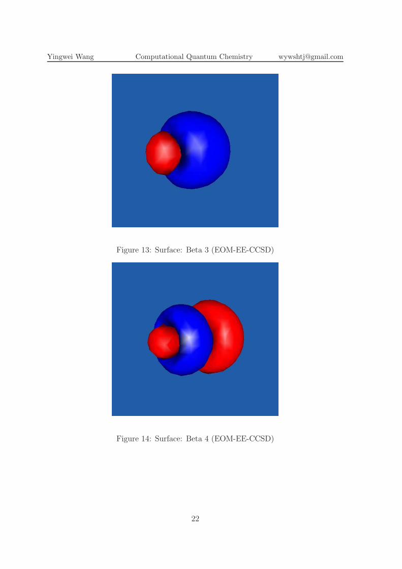
Figure 13: Surface: Beta 3 (EOM-EE-CCSD)
Figure 14: Surface: Beta 4 (EOM-EE-CCSD)
22
Yingwei Wang Computational Quantum Chemistry [email protected]
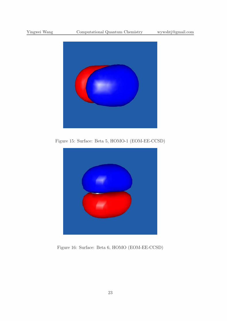
Figure 15: Surface: Beta 5, HOMO-1 (EOM-EE-CCSD)
Figure 16: Surface: Beta 6, HOMO (EOM-EE-CCSD)
23
Yingwei Wang Computational Quantum Chemistry [email protected]
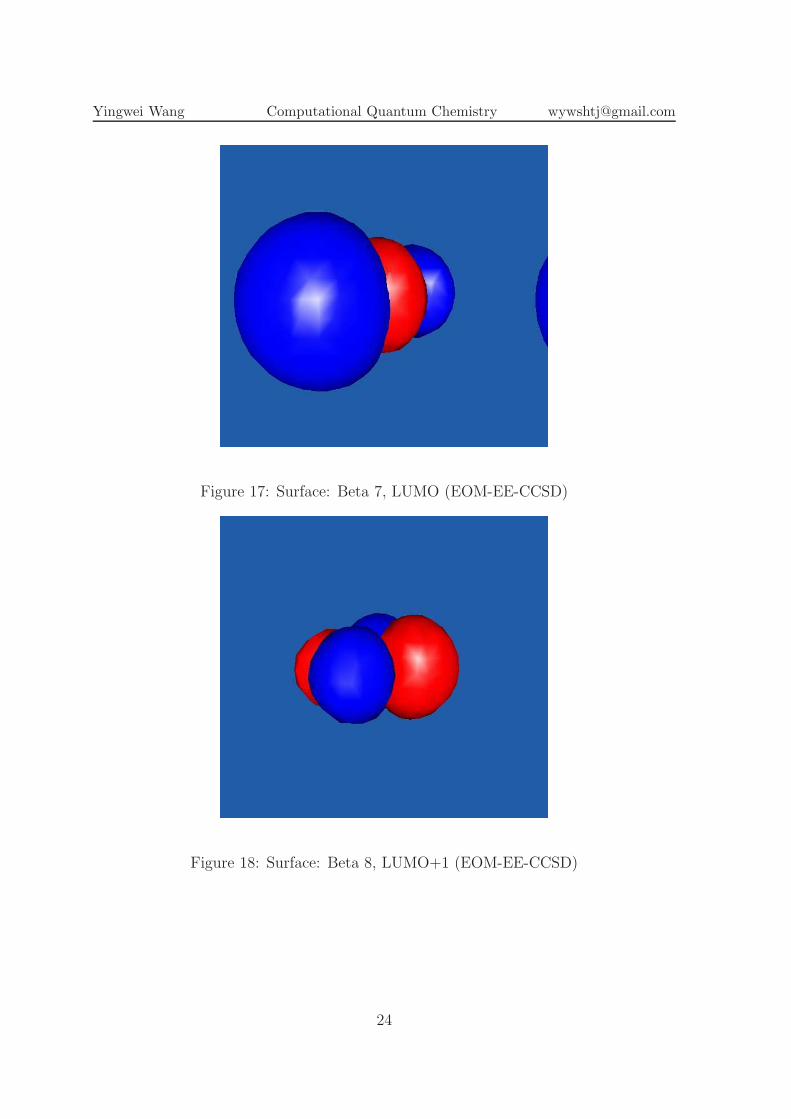
Figure 17: Surface: Beta 7, LUMO (EOM-EE-CCSD)
Figure 18: Surface: Beta 8, LUMO+1 (EOM-EE-CCSD)
24
Yingwei Wang Computational Quantum Chemistry [email protected]
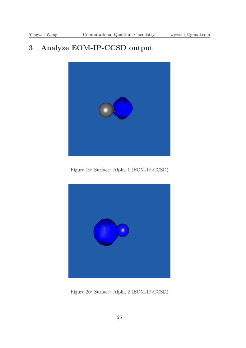
3 Analyze EOM-IP-CCSD output
Figure 19: Surface: Alpha 1 (EOM-IP-CCSD)
Figure 20: Surface: Alpha 2 (EOM-IP-CCSD)
25

Yingwei Wang Computational Quantum Chemistry [email protected]
Figure 21: Surface: Alpha 3 (EOM-IP-CCSD)
Figure 22: Surface: Alpha 4 (EOM-IP-CCSD)
26
Yingwei Wang Computational Quantum Chemistry [email protected]
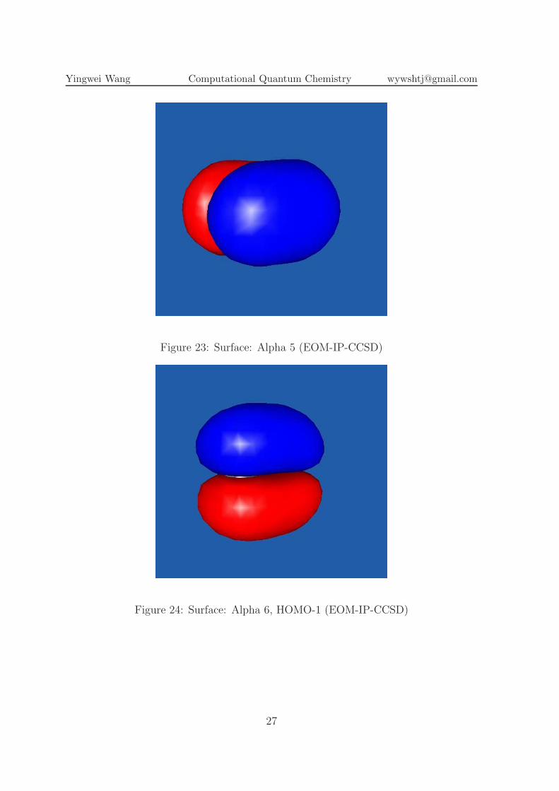
Figure 23: Surface: Alpha 5 (EOM-IP-CCSD)
Figure 24: Surface: Alpha 6, HOMO-1 (EOM-IP-CCSD)
27

Yingwei Wang Computational Quantum Chemistry [email protected]
Figure 25: Surface: Alpha 7, HOMO (EOM-IP-CCSD)
Figure 26: Surface: Alpha 8, LUMO (EOM-IP-CCSD)
28
Yingwei Wang Computational Quantum Chemistry [email protected]
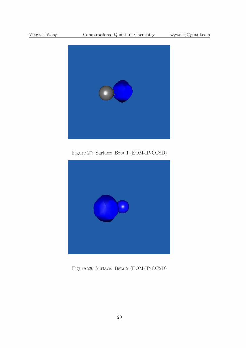
Figure 27: Surface: Beta 1 (EOM-IP-CCSD)
Figure 28: Surface: Beta 2 (EOM-IP-CCSD)
29
Yingwei Wang Computational Quantum Chemistry [email protected]
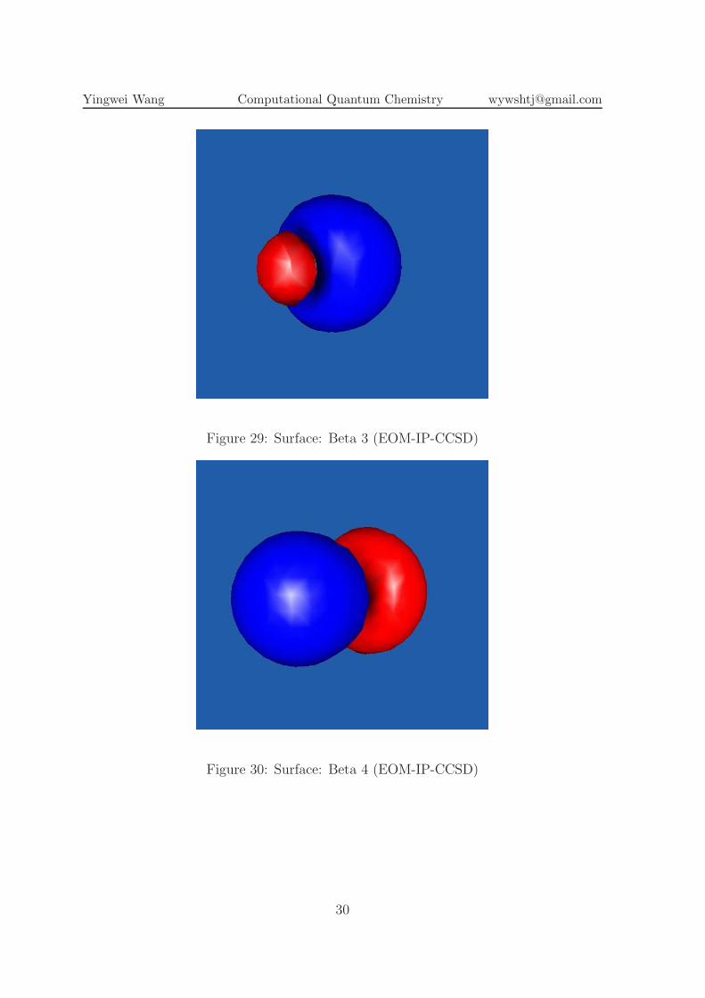
Figure 29: Surface: Beta 3 (EOM-IP-CCSD)
Figure 30: Surface: Beta 4 (EOM-IP-CCSD)
30

Yingwei Wang Computational Quantum Chemistry [email protected]
Figure 31: Surface: Beta 5 (EOM-IP-CCSD)
Figure 32: Surface: Beta 6, HOMO-1 (EOM-IP-CCSD)
31
Yingwei Wang Computational Quantum Chemistry [email protected]
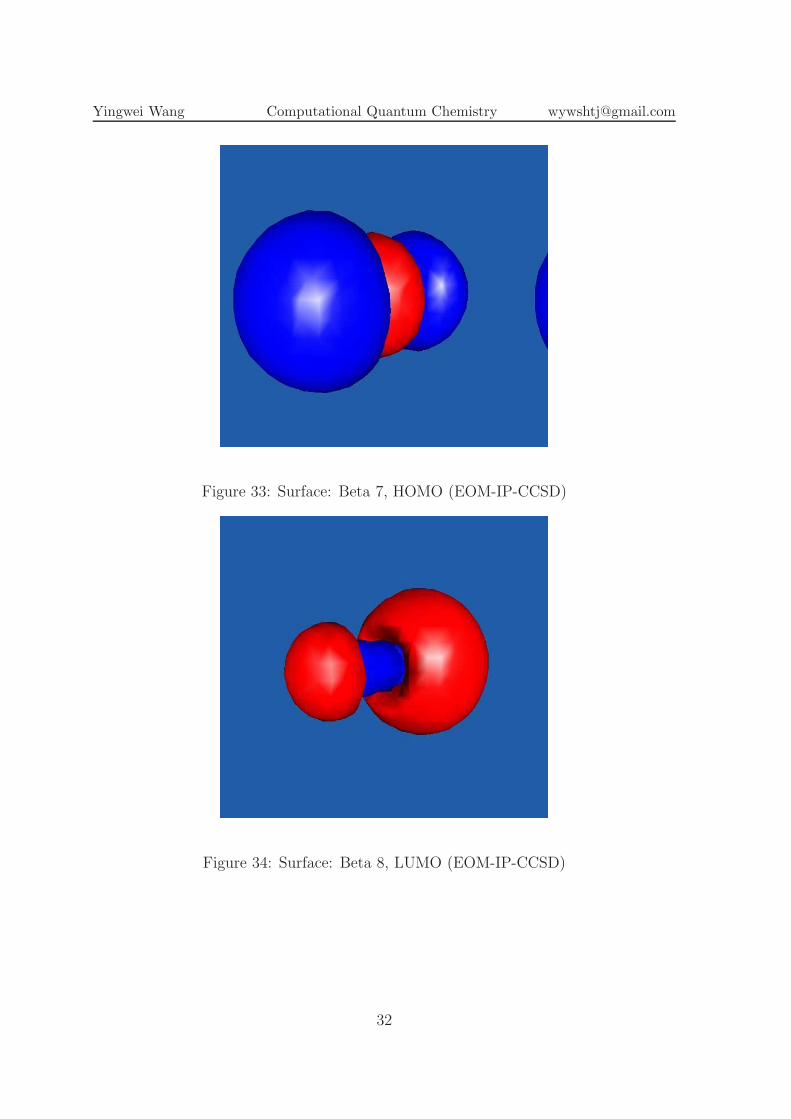
Figure 33: Surface: Beta 7, HOMO (EOM-IP-CCSD)
Figure 34: Surface: Beta 8, LUMO (EOM-IP-CCSD)
32
Yingwei Wang Computational Quantum Chemistry [email protected]
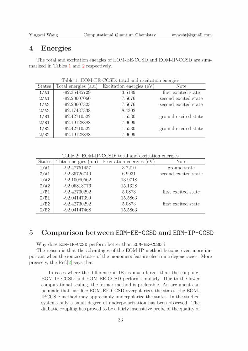
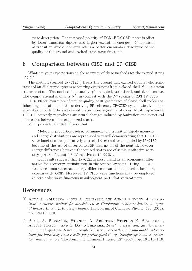
4 Energies
The total and excitation energies of EOM-EE-CCSD and EOM-IP-CCSD are sum-marized in Tables 1 and 2 respectively.
Table 1: EOM-EE-CCSD: total and excitation energiesStates Total energies (a.u) Excitation energies (eV) Note1/A1 -92.35485729 3.5189 first excited state2/A1 -92.20607060 7.5676 second excited state1/A2 -92.20607323 7.5676 second excited state2/A2 -92.17437338 8.43021/B1 -92.42710522 1.5530 ground excited state2/B1 -92.19128888 7.96991/B2 -92.42710522 1.5530 ground excited state2/B2 -92.19128888 7.9699
Table 2: EOM-IP-CCSD: total and excitation energiesStates Total energies (a.u) Excitation energies (eV) Note1/A1 -92.47751457 3.7210 ground state2/A1 -92.35726740 6.9931 second excited state1/A2 -92.10080562 13.97182/A2 -92.05813776 15.13281/B1 -92.42730292 5.0873 first excited state2/B1 -92.04147399 15.58631/B2 -92.42730292 5.0873 first excited state2/B2 -92.04147468 15.5863
5 Comparison between EOM-EE-CCSD and EOM-IP-CCSD
Why does EOM-IP-CCSD perform better than EOM-EE-CCSD ?The reason is that the advantages of the EOM-IP method become even more im-
portant when the ionized states of the monomers feature electronic degeneracies. Moreprecisely, the Ref.[2] says that
In cases where the difference in IEs is much larger than the coupling,EOM-IP-CCSD and EOM-EE-CCSD perform similarly. Due to the lowercomputational scaling, the former method is preferable. An argument canbe made that just like EOM-EE-CCSD overpolarizes the states, the EOM-IPCCSD method may appreciably underpolarize the states. In the studiedsystems only a small degree of underpolarization has been observed. Thediabatic coupling has proved to be a fairly insensitive probe of the quality of
33
Yingwei Wang Computational Quantum Chemistry [email protected]
state description. The increased polarity of EOM-EE-CCSD states is offsetby lower transition dipoles and higher excitation energies. Comparisonof transition dipole moments offers a better onenumber descriptor of thequality of the ground and excited state wave functions.
6 Comparison between CISD and IP-CISD
What are your expectations on the accuracy of these methods for the excited statesof CN?
The method (termed IP-CISD ) treats the ground and excited doublet electronicstates of an N -electron system as ionizing excitations from a closed-shell N+1-electronreference state. The method is naturally spin adapted, variational, and size intensive.The computational scaling is N5, in contrast with the N6 scaling of EOM-IP-CCSD.
IP-CISD structures are of similar quality as HF geometries of closed-shell molecules.Inheriting limitations of the underlying HF reference, IP-CISD systematically under-estimates bond lengths and overestimates interfragment distances. Most importantly,IP-CISD correctly reproduces structural changes induced by ionization and structuraldifferences between different ionized states.
More precisely, the Ref.[1] says that
Molecular properties such as permanent and transition dipole momentsand charge distributions are reproduced very well demonstrating that IP-CISDwave functions are qualitatively correct. IEs cannot be computed by IP-CISDbecause of the use of uncorrelated HF description of the neutral, however,energy differences between the ionized states are of semiquantitative accu-racy (errors of about 0.3 eV relative to IP-CCSD).
Our results suggest that IP-CISD is most useful as an economical alter-native for geometry optimization in the ionized systems. Using IP-CISD
structures, more accurate energy differences can be computed using moreexpensive IP-CCSD. Moreover, IP-CISD wave functions may be employedas zero-order wave functions in subsequent perturbative treatment.
References
[1] Anna A. Golubeva, Piotr A. Pieniazek, and Anna I. Krylov, A new elec-
tronic structure method for doublet states: Configuration interaction in the space
of ionized 1h and 2h1p determinants, The Journal of Chemical Physics, 130 (2009),pp. 124113–1,10.
[2] Piotr A. Pieniazek, Stephen A. Arnstein, Stephen E. Bradforth,
Anna I. Krylov, and C. David Sherrill, Benchmark full configuration inter-
action and equation-of-motion coupled-cluster model with single and double substitu-
tions for ionized systems results for prototypical charge transfer systems: Noncova-
lent ionized dimers, The Journal of Chemical Physics, 127 (2007), pp. 164110–1,19.
34