Homework 8 Solutions

Chapter 14

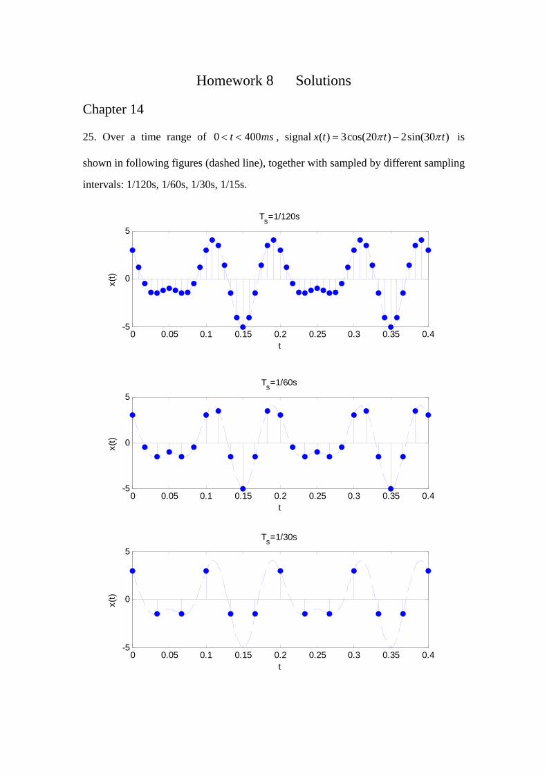
25. Over a time range of 0 400t ms< < , signal ( ) 3cos(20 ) 2sin(30 )x t t tπ π= − is

shown in following figures (dashed line), together with sampled by different sampling

intervals: 1/120s, 1/60s, 1/30s, 1/15s.

0 0.05 0.1 0.15 0.2 0.25 0.3 0.35 0.4-5

0

5

t

x(t)

Ts=1/120s

1/60

0 0.05 0.1 0.15 0.2 0.25 0.3 0.35 0.4-5

0

5

t

x(t)

Ts=1/60s

0 0.05 0.1 0.15 0.2 0.25 0.3 0.35 0.4-5

0

5

t

x(t)

Ts=1/30s

T 1/1

0 0.05 0.1 0.15 0.2 0.25 0.3 0.35 0.4-5

0

5

t

x(t)

Ts=1/15s

From four figures shown above, this signal can be reconstructed when sampled by

1/120sT s= , 1/ 60sT s= and cannot be reconstructed for 1/ 30sT s= , 1/15sT s= .

Analytically, we can determine if the signal can be reconstructed by finding its Nyquist rate.

( ) 3cos(20 ) 2sin(30 )x t t tπ π= −

↔3[ ] [ ( 10) ( 10)] [ ( 15) ( 15)]2

X f f f j f fδ δ δ δ= − + + + − − +

So, 15Hzmf = , 2 30HzNyq mf f= = . In order to reconstruct the signal, sampling

frequency should satisfy: 30Hzs Nyqf f> = ⇒ 1/ 30sT s<

CODE: clear all; t = 0:1e-3:400e-3; y0 = 3*cos(20*pi*t)-2*sin(30*pi*t); figure(1), subplot(2,1,1),plot(t,y0,'--'); xlabel('t');ylabel('x(t)'),hold on subplot(2,1,2),plot(t,y0,'--'); xlabel('t');ylabel('x(t)'),hold on figure(2), subplot(2,1,1),plot(t,y0,'--'); xlabel('t');ylabel('x(t)'),hold on subplot(2,1,2),plot(t,y0,'--'); xlabel('t');ylabel('x(t)'),hold on t1 = 0:1/120:400e-3; % (a) Ts = 1/120s; y1 = 3*cos(20*pi*t1)-2*sin(30*pi*t1); figure(1) subplot(2,1,1),stem(t1,y1,'fill'); title('T_s=1/120s'),hold off t2 = 0:1/60:400e-3; % (b) Ts = 1/60s;

y2 = 3*cos(20*pi*t2)-2*sin(30*pi*t2); figure(1) subplot(2,1,2),stem(t2,y2,'fill'); title('T_s=1/60s'),hold off t3 = 0:1/30:400e-3; % (c) Ts = 1/30s; y3 = 3*cos(20*pi*t3)-2*sin(30*pi*t3); figure(2) subplot(2,1,1),stem(t3,y3,'fill'); title('T_s=1/30s'),hold off t4 = 0:1/15:400e-3; % (d) Ts = 1/15s; y4 = 3*cos(20*pi*t4)-2*sin(30*pi*t4); figure(2) subplot(2,1,2),stem(t4,y4,'fill'); title('T_s=1/15s'),hold off

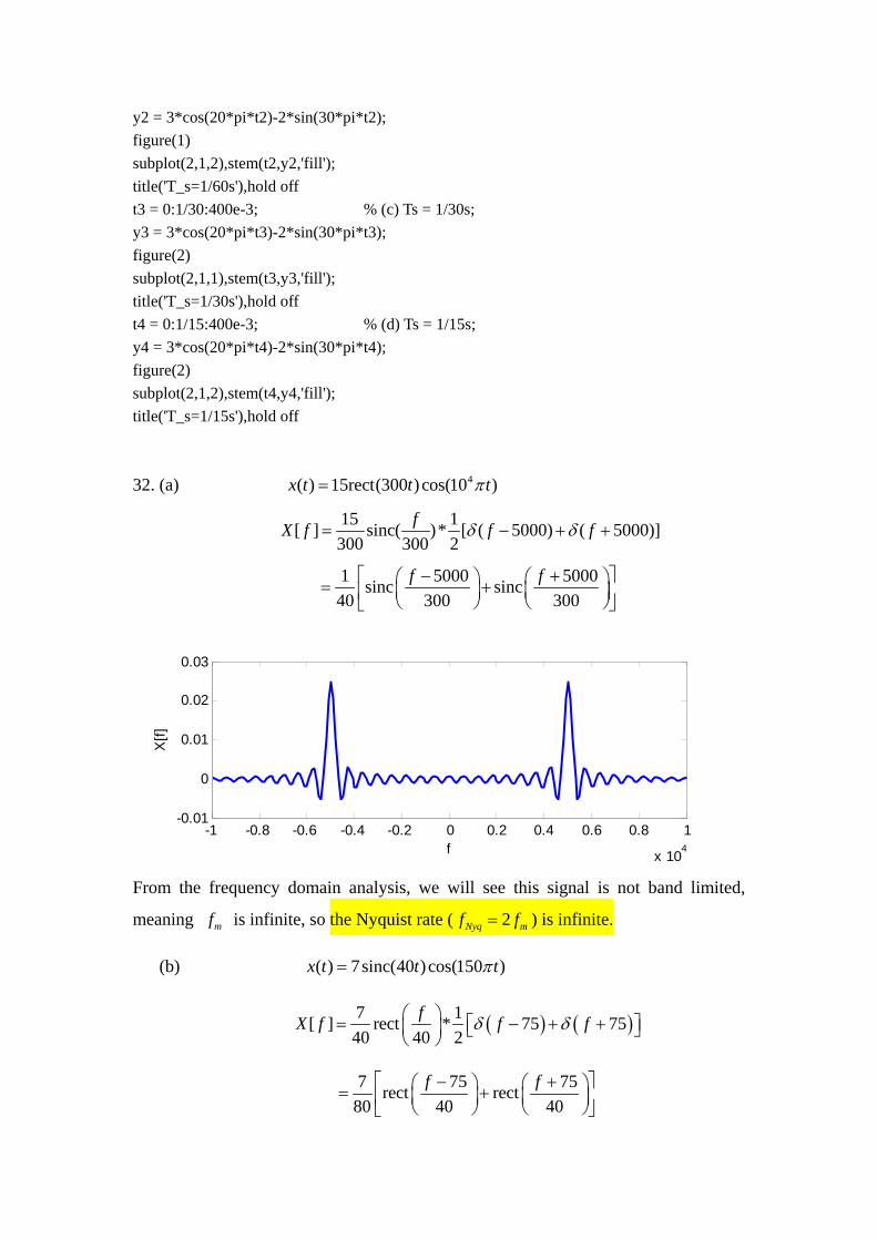
32. (a) 4( ) 15rect(300 )cos(10 )x t t tπ=

15 1[ ] sinc( )* [ ( 5000) ( 5000)]300 300 2

fX f f fδ δ= − + +

1 5000 5000sinc sinc40 300 300

f f⎡ − + ⎤⎛ ⎞ ⎛ ⎞= +⎜ ⎟ ⎜ ⎟⎢ ⎥⎝ ⎠ ⎝ ⎠⎣ ⎦

-1 -0.8 -0.6 -0.4 -0.2 0 0.2 0.4 0.6 0.8 1

x 104

-0.01

0

0.01

0.02

0.03

f

X[f]

From the frequency domain analysis, we will see this signal is not band limited,

meaning mf is infinite, so the Nyquist rate ( 2Nyq mf f= ) is infinite.

(b) ( ) 7sinc(40 )cos(150 )x t t tπ=

( ) ( )7 1[ ] rect * 75 7540 40 2

fX f f fδ δ⎛ ⎞= − + +⎡ ⎤⎜ ⎟ ⎣ ⎦⎝ ⎠

7 75 75rect rect80 40 40

f f⎡ − + ⎤⎛ ⎞ ⎛ ⎞= +⎜ ⎟ ⎜ ⎟⎢ ⎥⎝ ⎠ ⎝ ⎠⎣ ⎦

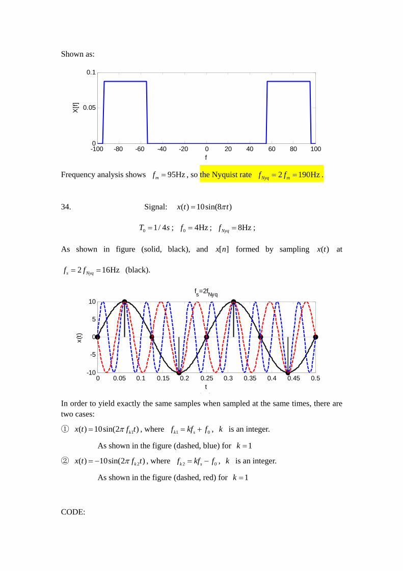
Shown as:

-100 -80 -60 -40 -20 0 20 40 60 80 1000

0.05

0.1

f

X[f]

Frequency analysis shows 95Hzmf = , so the Nyquist rate 2 190HzNyq mf f= = .

34. Signal: ( ) 10sin(8 )x t tπ=

0 1/ 4T s= ; 0 4Hzf = ; 8HzNyqf = ;

As shown in figure (solid, black), and [ ]x n formed by sampling ( )x t at

2 16Hzs Nyqf f= = (black).

0 0.05 0.1 0.15 0.2 0.25 0.3 0.35 0.4 0.45 0.5-10

-5

0

5

10

t

x(t)

fs=2fNyq

f f

In order to yield exactly the same samples when sampled at the same times, there are two cases:

① 1( ) 10sin(2 )kx t f tπ= , where 1 0k sf kf f= + , k is an integer.

As shown in the figure (dashed, blue) for 1k =

② 2( ) 10sin(2 )kx t f tπ= − , where 2 0k sf kf f= − , k is an integer.

As shown in the figure (dashed, red) for 1k =

CODE:

clear all, t = 0:0.001:0.5; y0 = 10*sin(8*pi*t); figure(1),subplot(2,1,1),plot(t,y0,'-k') xlabel('t'),ylabel('x(t)'),hold on t1 = 0:1/16:0.5; y1 = 10*sin(8*pi*t1); %Sample at twice Nyquist rate figure(1),subplot(2,1,1),stem(t1,y1,'fill','k'); title('f_s=2f_{Nyq}'), y1_1 = 10*sin(40*pi*t); %T1=1/20, yields the same sample as original one figure(1),subplot(2,1,1),plot(t,y1_1,'--b'); y1_2 = -10*sin(24*pi*t); %T1=1/12, yields the same sample as original one figure(1),subplot(2,1,1),plot(t,y1_2,'--r'); hold off

39. (a) ( ) 8 3cos(8 ) 9sin(4 )x t t tπ π= + +

The period of this signal should be the least common multiple of 14

(the period of

cos(8 )tπ ) and 12

(the period of sin(4 )tπ ), which yields 012

T s= . By frequency analysis,

we can find 4Hzmf = , so 2 8HzNyq mf f= = . In order to exactly describe the signal,

sampling frequency sf should larger than Nyquist rate Nyqf . Within a period of 12

s ,

sample values should larger than 01 8 42NyqT f = ⋅ = and must be a integer, which

yields to 5. So we need 5 samples within one period of 0T and 05 / 10Hzsf T= = .

(b) ( ) 8 3cos(7 ) 9sin(4 )x t t tπ π= + +

Similar to the part (a), The period 0T is the least common multiple of 27

(the period of

cos(7 )tπ ) and 12

(the period of sin(4 )tπ ), which yields 0 2T s= . By frequency analysis,

we can find 3.5Hzmf = , so 2 7HzNyq mf f= = . In order to exactly describe the signal,

sampling frequency sf should larger than Nyquist rate Nyqf . Within a period of 2s ,

sample values should larger than 0 2 7 14NyqT f = ⋅ = and must be a integer, which

yields to 15. So we need 15 samples within one period of 2s and

015 / 7.5Hzsf T= = .

44. ( ) 15cos(300 ) 40sin(200 )x t t tπ π= +

The period of the signal is: 01 1 1LCM ,

150 100 50T s⎧ ⎫= =⎨ ⎬

⎩ ⎭

150Hzmf = , 2 300HzNyq mf f= =

(a) 300Hzs Nyqf f= =

Number of samples within one period is: 0 01 300 650sN T f= = ⋅ =

So, sampling ( )x t at 00 300

n nt TN

= = , 0,1,2,3,4,5n = , as shown in the figure.

[ ]x n : [15, 19.64, -19.64, -15, 49.64, -49.64]

DFT: 0

0

21

0[ ] [ ]

nkN jN

DFTn

X k x n eπ− −

=

= ∑

⇒ [ ]DFTX k : [0, 0, -j120, 90, j120, 0]

This can also be calculated in Matlab by commend “fft(x_n)”

CTFS: 0

[ ][ ] DFTCTFS

X kX kN

=

Note that calculate [ ]CTFSX k for k from 0 / 2N− to 0 / 2N , while [ ]DFTX k is for

k from 0 to 0 1N − , so periodicity of [ ]DFTX k is used here. The starting point at

0 / 2N− and ending point at 0 / 2N are actually repeated, which means the last point

in one period of 0N will overlap the first point in the next period. We need to ensure

value after such overlap still fix at 0

0

[ / 2]DFTX NN

, so

0 0 0

0

[ / 2]2 2 2

DFTCTFS CTFS

N N X NX XN

⎡ ⎤ ⎡ ⎤− = =⎢ ⎥ ⎢ ⎥⎣ ⎦ ⎣ ⎦

⇒ [ ]CTFSX k : [7.5, j20, 0, 0, 0, -j20, 7.5]

The CTFS representation of the signal is:

00

0

/2 32 ( ) 100

/2 3

( ) [ ] [ ]N

j kf t j ktCTFS CTFS

k N k

x t X k e X k eπ π

=− =−

= =∑ ∑

As shown in the figure, the CTFS representation of the signal looks same as the original signal.

0 0.002 0.004 0.006 0.008 0.01 0.012 0.014 0.016 0.018 0.02-100

-50

0

50

100fs=fNyq

t

x(t)

and

x(n)

0 0.002 0.004 0.006 0.008 0.01 0.012 0.014 0.016 0.018 0.02-100

-50

0

50

100

t

x(t)

from

CTF

S

CODE: clear all, N0 = 6; % 6 samples within one period n = 0:1/50/N0:1/50-1/50/N0; x_n = 15*cos(300*pi*n)+40*sin(200*pi*n), x_DFT = fft(x_n), % get DFT of the samples x_CTFS = 1/N0*[x_DFT(4)/2,x_DFT(5:6),x_DFT(1),x_DFT(2:3),x_DFT(4)/2], % get CTFS of the samples t = 0:1/50/100:1/50; x_t1 = 15*cos(300*pi*t)+40*sin(200*pi*t); x_t2 = 0; for nn = -N0/2:N0/2; x_t2 = x_t2+x_CTFS(nn+N0/2+1)*exp(j*(nn)*2*pi*50*t); end figure(1),subplot(2,1,1),plot(t,x_t1) %original x(t) title('f_s=f_{Nyq}'),xlabel('t'),ylabel('x(t) and x(n)'), hold on subplot(2,1,1),stem(n,x_n,'fill'),hold off %samples x(n)

figure(1),subplot(2,1,2),plot(t,x_t2) %CTFS representation of the signal xlabel('t'),ylabel('x(t) from CTFS'),

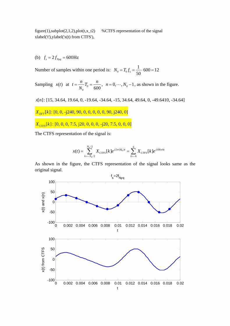
(b) 2 600Hzs Nyqf f= =

Number of samples within one period is: 0 01 600 1250sN T f= = ⋅ =

Sampling ( )x t at 00 600

n nt TN

= = , 00, , 1n N= −L , as shown in the figure.

[ ]x n : [15, 34.64, 19.64, 0, -19.64, -34.64, -15, 34.64, 49.64, 0, -49.6410, -34.64]

[ ]DFTX k : [0, 0, -j240, 90, 0, 0, 0, 0, 0, 90, j240, 0]

[ ]CTFSX k : [0, 0, 0, 7.5, j20, 0, 0, 0, -j20, 7.5, 0, 0, 0]

The CTFS representation of the signal is:

00

0

/2 62 ( ) 100

/2 6

( ) [ ] [ ]N

j kf t j ktCTFS CTFS

k N k

x t X k e X k eπ π

=− =−

= =∑ ∑

As shown in the figure, the CTFS representation of the signal looks same as the original signal.

0 0.002 0.004 0.006 0.008 0.01 0.012 0.014 0.016 0.018 0.02-100

-50

0

50

100fs=2fNyq

t

x(t)

and

x(n)

0 0.002 0.004 0.006 0.008 0.01 0.012 0.014 0.016 0.018 0.02-100

-50

0

50

100

t

x(t)

from

CTF

S

CODE: clear all, N0 = 12; % 12 samples within one period n = 0:1/50/N0:1/50-1/50/N0; x_n = 15*cos(300*pi*n)+40*sin(200*pi*n), x_DFT = fft(x_n), % get DFT of the samples x_CTFS = 1/N0*[x_DFT(7)/2,x_DFT(8:12),x_DFT(1),x_DFT(2:6),x_DFT(7)/2], % get CTFS of the samples t = 0:1/50/100:1/50; x_t1 = 15*cos(300*pi*t)+40*sin(200*pi*t); x_t2 = 0; for nn = -N0/2:N0/2; x_t2 = x_t2+x_CTFS(nn+N0/2+1)*exp(j*(nn)*2*pi*50*t); end figure(2),subplot(2,1,1),plot(t,x_t1) %original x(t) title('f_s=2f_{Nyq}'),xlabel('t'),ylabel('x(t) and x(n)'), hold on subplot(2,1,1),stem(n,x_n,'fill'),hold off %samples x(n) figure(2),subplot(2,1,2),plot(t,x_t2) %CTFS representation of the signal xlabel('t'),ylabel('x(t) from CTFS'),