Homework 1 solutions

Joe Neeman

September 10, 2010

1. To check that {Xt} is white noise, we need to compute its means andcovariances. For the means, EXt = EWt(1 − Wt−1)Zt = (EWt)(1 −EWt−1)(EZt) = 0. For the covariances,

γ(s, t) = E(

Ws(1 − Ws−1)ZsWt(1 − Wt−1)Zt

)

= E(

Ws(1 − Ws−1)Wt(1 − Wt−1))

· EZsZt.

If s 6= t then the last term is EZsZt = EZs · EZt = 0. Therefore {Xt} isuncorrelated. If s = t then EZsZt = EZ2

t = 1 and so

γ(t, t) = EW 2t(1 − Wt−1)

2 =1

4.

Thus, {Xt} has constant variance. Hence it is white noise.

To show that {Xt} is not i.i.d, note that Xt−1 = 1 implies that Wt−1 = 1,which implies that Xt = 0. Therefore

P (Xt−1 = 1, Xt = 1) = 0.

Since this is not equal to P (Xt−1 = 1)P (Xt = 1) = 1/64, Xt and Xt−1

are not independent.

2. (a) Xt = Wt − Wt−3 is a stationary process: EXt = EWt − EWt−3 = 0and

γ(s, t) = EXsXt = EWsWt + EWsWt−3 + EWs−3Wt + EWs−3Wt−3

= 1{s=t} + ·1{s=t−3} + ·1{s−3=t} + ·1{s−3=t−3}

= 2 · 1{|s−t|=0} + 1{|s−t|=3},

which is a function of |s − t|.

(b) Xt = W3 is a stationary process because EXt = EW3 = 0 andEXsXt = EW 2

3 = 1.

(c) Xt = W3 + t is not a stationary process because its mean is notconstant: EXt = t.

1

Homework 1 solutions, Fall 2010 Joe Neeman

(d) Xt = W 2t

is a stationary process: EXt = EW 2t

= 1 and

EXsXt = EW 2sW 2

t=

{

3 if s = t

1 if s 6= t.

(e) Xt = WtWt−2 is a stationary process: EXt = EWtEWt−2 = 0 andγ(s, t) = EWsWs−2WtWt−2 = 1{s=t}.

3. If Xt = Wt−1 + 2Wt + Wt+1, then

γ(t, t) = E(Wt−1 + 2Wt + Wt+1)2 = EW 2

t−1 + 4EW 2t + EW 2

t+1 = 6σ2w

γ(t, t + 1) = E(Wt−1 + 2Wt + Wt+1)(Wt + 2Wt+1 + Wt+2)

= 2EW 2t

+ 2EW 2t+1 = 4σ2

w

γ(t, t + 2) = E(Wt−1 + 2Wt + Wt+1)(Wt+1 + 2Wt+2 + Wt+3)

= EW 2t+1 = σ2

w

and γ(t, t + h) = 0 for h ≥ 3. By symmetry, γ(t, t − h) = γ(t, t + h).

For the autocorrelation function, we saw above that γ(t, t) = 6σ2w for all

t. Therefore,

ρ(h) =γ(t, t + h)

γ(t, t)

and so ρ(0) = 1, ρ(1) = 2/3, ρ(2) = 1/6 and ρ(h) = 0 for h ≥ 3.

The plots of the autocorrelation and autocovariance are shown in Figure 1

4. (a) If we differentiate with respect to A, we obtain

d

dAMSE(A) =

d

dA(EX2

t+ℓ+ A2

EX2t− 2AEXtXt+ℓ)

= 2AEX2t− 2EXtXt+ℓ

= 2Aγ(0) − 2γ(ℓ).

Setting this to zero, we see that the minimum is obtained at A =γ(ℓ)/γ(0) = ρ(ℓ).

(b) Plugging A = ρ(ℓ) back into the expression for MSE, we have

MSE(A) = γ(0) + ρ2(ℓ)γ(0) − 2ρ(ℓ)γ(ℓ) = γ(0)(1 − ρ2(ℓ))

since γ(ℓ) = ρ(ℓ)γ(0).

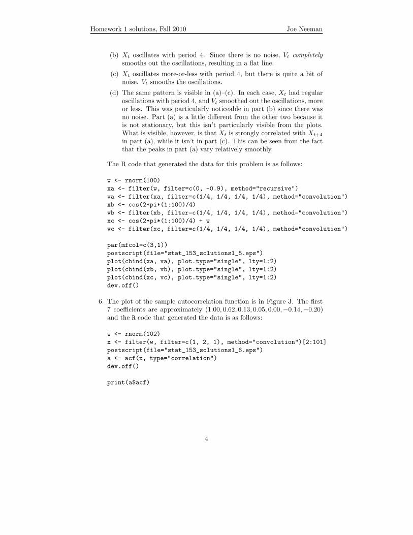
5. The plots for this problem are shown in Figure 2

(a) Xt oscillates regularly, with period about 4. This is to be expectedbecause Xt is strongly negatively correlated with Xt−2. In Vt, theoscillations are smoothed out.

2

Homework 1 solutions, Fall 2010 Joe Neeman

1 2 3 4 5

01

23

45

6

Autocovariance

lag

times

sig

ma_

w^2

1 2 3 4 5

0.0

0.2

0.4

0.6

0.8

1.0

Autocorrelation

lag

corr

elat

ion

Figure 1: Autocorrelation and autocovariance plots for Problem 3.

0 20 40 60 80 100

−4

−2

02

4

Time

0 20 40 60 80 100

−1.

0−

0.5

0.0

0.5

1.0

Time

0 20 40 60 80 100

−3

−2

−1

01

2

Time

Figure 2: Plots for Problem 5.

3

Homework 1 solutions, Fall 2010 Joe Neeman

(b) Xt oscillates with period 4. Since there is no noise, Vt completely

smooths out the oscillations, resulting in a flat line.

(c) Xt oscillates more-or-less with period 4, but there is quite a bit ofnoise. Vt smooths the oscillations.

(d) The same pattern is visible in (a)–(c). In each case, Xt had regularoscillations with period 4, and Vt smoothed out the oscillations, moreor less. This was particularly noticeable in part (b) since there wasno noise. Part (a) is a little different from the other two because itis not stationary, but this isn’t particularly visible from the plots.What is visible, however, is that Xt is strongly correlated with Xt+4

in part (a), while it isn’t in part (c). This can be seen from the factthat the peaks in part (a) vary relatively smoothly.

The R code that generated the data for this problem is as follows:

w <- rnorm(100)

xa <- filter(w, filter=c(0, -0.9), method="recursive")

va <- filter(xa, filter=c(1/4, 1/4, 1/4, 1/4), method="convolution")

xb <- cos(2*pi*(1:100)/4)

vb <- filter(xb, filter=c(1/4, 1/4, 1/4, 1/4), method="convolution")

xc <- cos(2*pi*(1:100)/4) + w

vc <- filter(xc, filter=c(1/4, 1/4, 1/4, 1/4), method="convolution")

par(mfcol=c(3,1))

postscript(file="stat_153_solutions1_5.eps")

plot(cbind(xa, va), plot.type="single", lty=1:2)

plot(cbind(xb, vb), plot.type="single", lty=1:2)

plot(cbind(xc, vc), plot.type="single", lty=1:2)

dev.off()

6. The plot of the sample autocorrelation function is in Figure 3. The first7 coefficients are approximately (1.00, 0.62, 0.13, 0.05, 0.00,−0.14,−0.20)and the R code that generated the data is as follows:

w <- rnorm(102)

x <- filter(w, filter=c(1, 2, 1), method="convolution")[2:101]

postscript(file="stat_153_solutions1_6.eps")

a <- acf(x, type="correlation")

dev.off()

print(a$acf)

4

Homework 1 solutions, Fall 2010 Joe Neeman

0 5 10 15 20

−0.

20.

00.

20.

40.

60.

81.

0

Lag

AC

F

Series x

Figure 3: Sample autocorrelation function for Problem 6.

5