Holomorphic symplectic geometry - math.unice.frbeauvill/conf/Lisbon.pdf · Holomorphic symplectic...
136
Holomorphic symplectic geometry Arnaud Beauville Universit´ e de Nice Lisbon, March 2011 Arnaud Beauville Holomorphic symplectic geometry
Transcript of Holomorphic symplectic geometry - math.unice.frbeauvill/conf/Lisbon.pdf · Holomorphic symplectic...
Holomorphic symplectic geometry
Arnaud Beauville
Universite de Nice
Lisbon, March 2011
Arnaud Beauville Holomorphic symplectic geometry
I. Symplectic structure
Definition
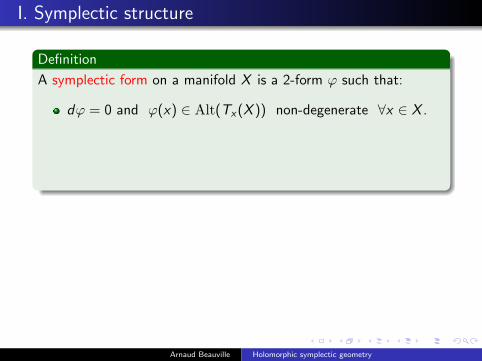
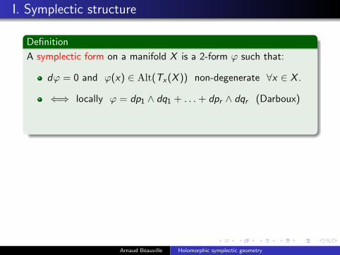
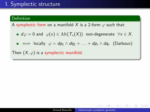
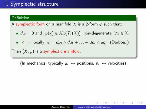
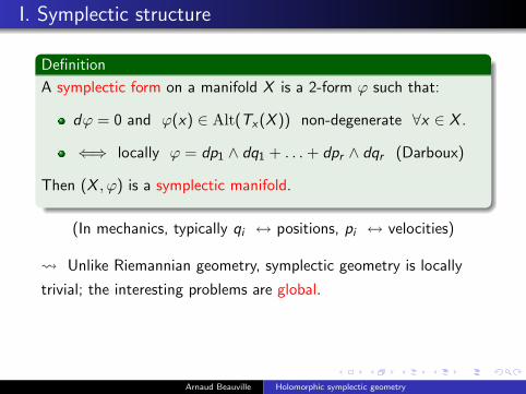
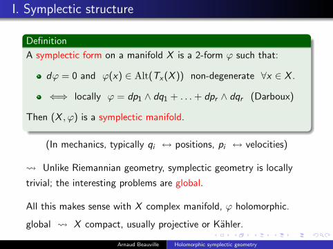
A symplectic form on a manifold X is a 2-form ϕ such that:
dϕ = 0 and ϕ(x) ∈ Alt(Tx(X )) non-degenerate ∀x ∈ X .
⇐⇒ locally ϕ = dp1 ∧ dq1 + . . .+ dpr ∧ dqr (Darboux)
Then (X , ϕ) is a symplectic manifold.
(In mechanics, typically qi ↔ positions, pi ↔ velocities)
Unlike Riemannian geometry, symplectic geometry is locally
trivial; the interesting problems are global.
All this makes sense with X complex manifold, ϕ holomorphic.
global X compact, usually projective or Kahler.
Arnaud Beauville Holomorphic symplectic geometry
I. Symplectic structure
Definition
A symplectic form on a manifold X is a 2-form ϕ such that:
dϕ = 0 and ϕ(x) ∈ Alt(Tx(X )) non-degenerate ∀x ∈ X .
⇐⇒ locally ϕ = dp1 ∧ dq1 + . . .+ dpr ∧ dqr (Darboux)
Then (X , ϕ) is a symplectic manifold.
(In mechanics, typically qi ↔ positions, pi ↔ velocities)
Unlike Riemannian geometry, symplectic geometry is locally
trivial; the interesting problems are global.
All this makes sense with X complex manifold, ϕ holomorphic.
global X compact, usually projective or Kahler.
Arnaud Beauville Holomorphic symplectic geometry
Holomorphic symplectic manifolds
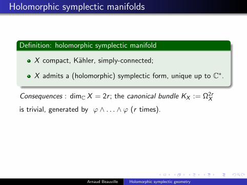
Definition: holomorphic symplectic manifold
X compact, Kahler, simply-connected;
X admits a (holomorphic) symplectic form, unique up to C∗.
Consequences : dimC X = 2r ; the canonical bundle KX := Ω2rX
is trivial, generated by ϕ ∧ . . . ∧ ϕ (r times).
(Note : on X compact Kahler, holomorphic forms are closed)
Why is it interesting?
Arnaud Beauville Holomorphic symplectic geometry
Holomorphic symplectic manifolds
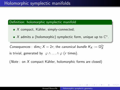
Definition: holomorphic symplectic manifold
X compact, Kahler, simply-connected;
X admits a (holomorphic) symplectic form, unique up to C∗.
Consequences : dimC X = 2r ; the canonical bundle KX := Ω2rX
is trivial, generated by ϕ ∧ . . . ∧ ϕ (r times).
(Note : on X compact Kahler, holomorphic forms are closed)
Why is it interesting?
Arnaud Beauville Holomorphic symplectic geometry
Holomorphic symplectic manifolds
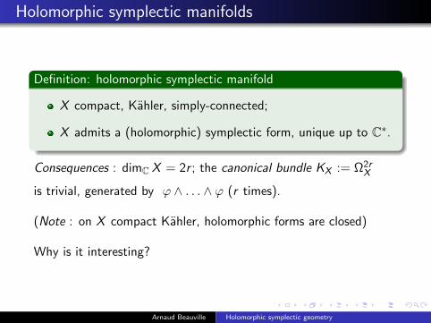
Definition: holomorphic symplectic manifold
X compact, Kahler, simply-connected;
X admits a (holomorphic) symplectic form, unique up to C∗.
Consequences : dimC X = 2r ; the canonical bundle KX := Ω2rX
is trivial, generated by ϕ ∧ . . . ∧ ϕ (r times).
(Note : on X compact Kahler, holomorphic forms are closed)
Why is it interesting?
Arnaud Beauville Holomorphic symplectic geometry
Holomorphic symplectic manifolds
Definition: holomorphic symplectic manifold
X compact, Kahler, simply-connected;
X admits a (holomorphic) symplectic form, unique up to C∗.
Consequences : dimC X = 2r ;
the canonical bundle KX := Ω2rX
is trivial, generated by ϕ ∧ . . . ∧ ϕ (r times).
(Note : on X compact Kahler, holomorphic forms are closed)
Why is it interesting?
Arnaud Beauville Holomorphic symplectic geometry
Holomorphic symplectic manifolds
Definition: holomorphic symplectic manifold
X compact, Kahler, simply-connected;
X admits a (holomorphic) symplectic form, unique up to C∗.
Consequences : dimC X = 2r ; the canonical bundle KX := Ω2rX
is trivial, generated by ϕ ∧ . . . ∧ ϕ (r times).
(Note : on X compact Kahler, holomorphic forms are closed)
Why is it interesting?
Arnaud Beauville Holomorphic symplectic geometry
Holomorphic symplectic manifolds
Definition: holomorphic symplectic manifold
X compact, Kahler, simply-connected;
X admits a (holomorphic) symplectic form, unique up to C∗.
Consequences : dimC X = 2r ; the canonical bundle KX := Ω2rX
is trivial, generated by ϕ ∧ . . . ∧ ϕ (r times).
(Note : on X compact Kahler, holomorphic forms are closed)
Why is it interesting?
Arnaud Beauville Holomorphic symplectic geometry
The Decomposition theorem
Decomposition theorem
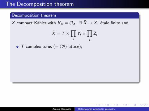
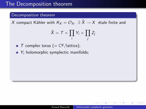
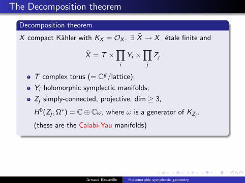
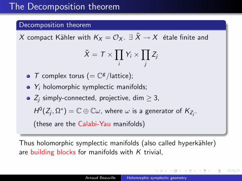
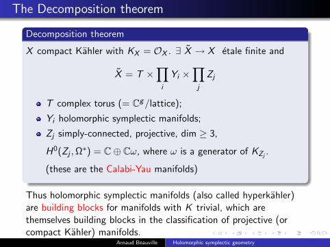
X compact Kahler with KX = OX . ∃ X → X etale finite and
X = T ×∏i
Yi ×∏j
Zj
T complex torus (= Cg/lattice);
Yi holomorphic symplectic manifolds;
Zj simply-connected, projective, dim ≥ 3,
H0(Zj ,Ω∗) = C⊕ Cω, where ω is a generator of KZj
.
(these are the Calabi-Yau manifolds)
Thus holomorphic symplectic manifolds (also called hyperkahler)are building blocks for manifolds with K trivial, which arethemselves building blocks in the classification of projective (orcompact Kahler) manifolds.
Arnaud Beauville Holomorphic symplectic geometry

The Decomposition theorem
Decomposition theorem
X compact Kahler with KX = OX . ∃ X → X etale finite and
X = T ×∏i
Yi ×∏j
Zj
T complex torus (= Cg/lattice);
Yi holomorphic symplectic manifolds;
Zj simply-connected, projective, dim ≥ 3,
H0(Zj ,Ω∗) = C⊕ Cω, where ω is a generator of KZj
.
(these are the Calabi-Yau manifolds)
Thus holomorphic symplectic manifolds (also called hyperkahler)are building blocks for manifolds with K trivial, which arethemselves building blocks in the classification of projective (orcompact Kahler) manifolds.
Arnaud Beauville Holomorphic symplectic geometry
The Decomposition theorem
Decomposition theorem
X compact Kahler with KX = OX . ∃ X → X etale finite and
X = T ×∏i
Yi ×∏j
Zj
T complex torus (= Cg/lattice);
Yi holomorphic symplectic manifolds;
Zj simply-connected, projective, dim ≥ 3,
H0(Zj ,Ω∗) = C⊕ Cω, where ω is a generator of KZj
.
(these are the Calabi-Yau manifolds)
Thus holomorphic symplectic manifolds (also called hyperkahler)are building blocks for manifolds with K trivial,
which arethemselves building blocks in the classification of projective (orcompact Kahler) manifolds.
Arnaud Beauville Holomorphic symplectic geometry
The Decomposition theorem
Decomposition theorem
X compact Kahler with KX = OX . ∃ X → X etale finite and
X = T ×∏i
Yi ×∏j
Zj
T complex torus (= Cg/lattice);
Yi holomorphic symplectic manifolds;
Zj simply-connected, projective, dim ≥ 3,
H0(Zj ,Ω∗) = C⊕ Cω, where ω is a generator of KZj
.
(these are the Calabi-Yau manifolds)
Thus holomorphic symplectic manifolds (also called hyperkahler)are building blocks for manifolds with K trivial, which arethemselves building blocks in the classification of projective (orcompact Kahler) manifolds.
Arnaud Beauville Holomorphic symplectic geometry
Examples?
Many examples of Calabi-Yau manifolds, very few of holomorphic
symplectic.
dim 2: X simply-connected, KX = OXdef⇐⇒ X K3 surface.
(Example: X ⊂ P3 of degree 4, etc.)
dim > 2? Idea: take S r for S K3. Many symplectic forms:
ϕ = λ1 p∗1ϕS + . . .+ λr p∗r ϕS , with λ1, . . . , λr ∈ C∗ .
Try to get unicity by imposing λ1 = . . . = λr , i.e.
ϕ invariant under Sr , i.e. ϕ comes from S (r) := S r/Sr =
subsets of r points of S , counted with multiplicities
S (r) is singular, but admits a natural desingularization S [r ] :=
finite analytic subspaces of S of length r (Hilbert scheme)
Arnaud Beauville Holomorphic symplectic geometry
Examples?
Many examples of Calabi-Yau manifolds,
very few of holomorphic
symplectic.
dim 2: X simply-connected, KX = OXdef⇐⇒ X K3 surface.
(Example: X ⊂ P3 of degree 4, etc.)
dim > 2? Idea: take S r for S K3. Many symplectic forms:
ϕ = λ1 p∗1ϕS + . . .+ λr p∗r ϕS , with λ1, . . . , λr ∈ C∗ .
Try to get unicity by imposing λ1 = . . . = λr , i.e.
ϕ invariant under Sr , i.e. ϕ comes from S (r) := S r/Sr =
subsets of r points of S , counted with multiplicities
S (r) is singular, but admits a natural desingularization S [r ] :=
finite analytic subspaces of S of length r (Hilbert scheme)
Arnaud Beauville Holomorphic symplectic geometry
Examples?
Many examples of Calabi-Yau manifolds, very few of holomorphic
symplectic.
dim 2: X simply-connected, KX = OXdef⇐⇒ X K3 surface.
(Example: X ⊂ P3 of degree 4, etc.)
dim > 2? Idea: take S r for S K3. Many symplectic forms:
ϕ = λ1 p∗1ϕS + . . .+ λr p∗r ϕS , with λ1, . . . , λr ∈ C∗ .
Try to get unicity by imposing λ1 = . . . = λr , i.e.
ϕ invariant under Sr , i.e. ϕ comes from S (r) := S r/Sr =
subsets of r points of S , counted with multiplicities
S (r) is singular, but admits a natural desingularization S [r ] :=
finite analytic subspaces of S of length r (Hilbert scheme)
Arnaud Beauville Holomorphic symplectic geometry
Examples?
Many examples of Calabi-Yau manifolds, very few of holomorphic
symplectic.
dim 2: X simply-connected, KX = OXdef⇐⇒ X K3 surface.
(Example: X ⊂ P3 of degree 4, etc.)
dim > 2? Idea: take S r for S K3. Many symplectic forms:
ϕ = λ1 p∗1ϕS + . . .+ λr p∗r ϕS , with λ1, . . . , λr ∈ C∗ .
Try to get unicity by imposing λ1 = . . . = λr , i.e.
ϕ invariant under Sr , i.e. ϕ comes from S (r) := S r/Sr =
subsets of r points of S , counted with multiplicities
S (r) is singular, but admits a natural desingularization S [r ] :=
finite analytic subspaces of S of length r (Hilbert scheme)
Arnaud Beauville Holomorphic symplectic geometry
Examples?
Many examples of Calabi-Yau manifolds, very few of holomorphic
symplectic.
dim 2: X simply-connected, KX = OXdef⇐⇒ X K3 surface.
(Example: X ⊂ P3 of degree 4, etc.)
dim > 2? Idea: take S r for S K3. Many symplectic forms:
ϕ = λ1 p∗1ϕS + . . .+ λr p∗r ϕS , with λ1, . . . , λr ∈ C∗ .
Try to get unicity by imposing λ1 = . . . = λr ,
i.e.
ϕ invariant under Sr , i.e. ϕ comes from S (r) := S r/Sr =
subsets of r points of S , counted with multiplicities
S (r) is singular, but admits a natural desingularization S [r ] :=
finite analytic subspaces of S of length r (Hilbert scheme)
Arnaud Beauville Holomorphic symplectic geometry
Examples?
Many examples of Calabi-Yau manifolds, very few of holomorphic
symplectic.
dim 2: X simply-connected, KX = OXdef⇐⇒ X K3 surface.
(Example: X ⊂ P3 of degree 4, etc.)
dim > 2? Idea: take S r for S K3. Many symplectic forms:
ϕ = λ1 p∗1ϕS + . . .+ λr p∗r ϕS , with λ1, . . . , λr ∈ C∗ .
Try to get unicity by imposing λ1 = . . . = λr , i.e.
ϕ invariant under Sr ,
i.e. ϕ comes from S (r) := S r/Sr =
subsets of r points of S , counted with multiplicities
S (r) is singular, but admits a natural desingularization S [r ] :=
finite analytic subspaces of S of length r (Hilbert scheme)
Arnaud Beauville Holomorphic symplectic geometry
Examples?
Many examples of Calabi-Yau manifolds, very few of holomorphic
symplectic.
dim 2: X simply-connected, KX = OXdef⇐⇒ X K3 surface.
(Example: X ⊂ P3 of degree 4, etc.)
dim > 2? Idea: take S r for S K3. Many symplectic forms:
ϕ = λ1 p∗1ϕS + . . .+ λr p∗r ϕS , with λ1, . . . , λr ∈ C∗ .
Try to get unicity by imposing λ1 = . . . = λr , i.e.
ϕ invariant under Sr , i.e. ϕ comes from S (r) := S r/Sr =
subsets of r points of S , counted with multiplicities
S (r) is singular, but admits a natural desingularization S [r ] :=
finite analytic subspaces of S of length r (Hilbert scheme)
Arnaud Beauville Holomorphic symplectic geometry
Examples?
Many examples of Calabi-Yau manifolds, very few of holomorphic
symplectic.
dim 2: X simply-connected, KX = OXdef⇐⇒ X K3 surface.
(Example: X ⊂ P3 of degree 4, etc.)
dim > 2? Idea: take S r for S K3. Many symplectic forms:
ϕ = λ1 p∗1ϕS + . . .+ λr p∗r ϕS , with λ1, . . . , λr ∈ C∗ .
Try to get unicity by imposing λ1 = . . . = λr , i.e.
ϕ invariant under Sr , i.e. ϕ comes from S (r) := S r/Sr =
subsets of r points of S , counted with multiplicities
S (r) is singular, but admits a natural desingularization S [r ] :=
finite analytic subspaces of S of length r (Hilbert scheme)
Arnaud Beauville Holomorphic symplectic geometry

Examples
Theorem
For S K3, S [r ] is holomorphic symplectic, of dimension 2r .
Other examples
1 Analogous construction with S = complex torus (dim. 2);
gives generalized Kummer manifold Kr of dimension 2r .
2 Two isolated examples by O’Grady, of dimension 6 and 10.
All other known examples belong to one of the above families!
Example: V ⊂ P5 cubic fourfold. F (V ) := lines contained in V is holomorphic symplectic, deformation of S [2] with S K3.
Arnaud Beauville Holomorphic symplectic geometry
The period map
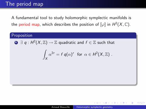
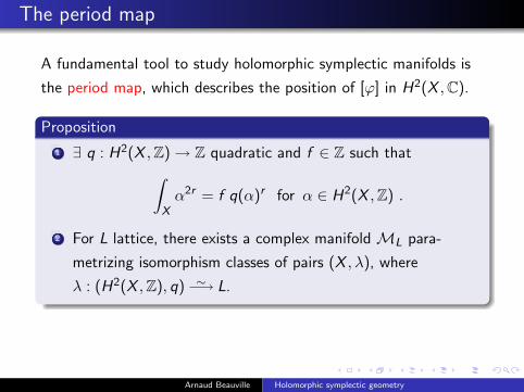
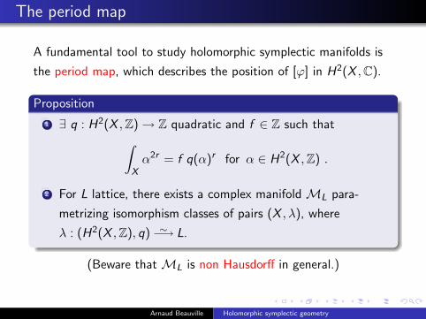
A fundamental tool to study holomorphic symplectic manifolds is
the period map, which describes the position of [ϕ] in H2(X ,C).
Proposition
1 ∃ q : H2(X ,Z)→ Z quadratic and f ∈ Z such that∫Xα2r = f q(α)r for α ∈ H2(X ,Z) .
2 For L lattice, there exists a complex manifold ML para-
metrizing isomorphism classes of pairs (X , λ), where
λ : (H2(X ,Z), q) ∼−→ L.
(Beware that ML is non Hausdorff in general.)
Arnaud Beauville Holomorphic symplectic geometry
The period map
A fundamental tool to study holomorphic symplectic manifolds is
the period map, which describes the position of [ϕ] in H2(X ,C).
Proposition
1 ∃ q : H2(X ,Z)→ Z quadratic and f ∈ Z such that∫Xα2r = f q(α)r for α ∈ H2(X ,Z) .
2 For L lattice, there exists a complex manifold ML para-
metrizing isomorphism classes of pairs (X , λ), where
λ : (H2(X ,Z), q) ∼−→ L.
(Beware that ML is non Hausdorff in general.)
Arnaud Beauville Holomorphic symplectic geometry
The period package
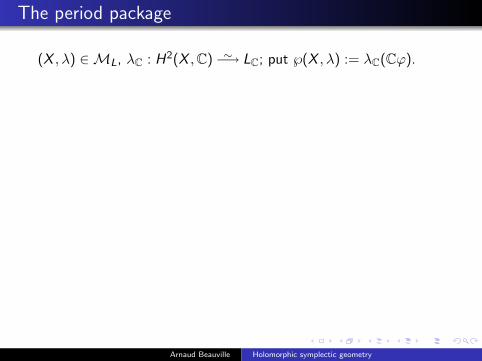
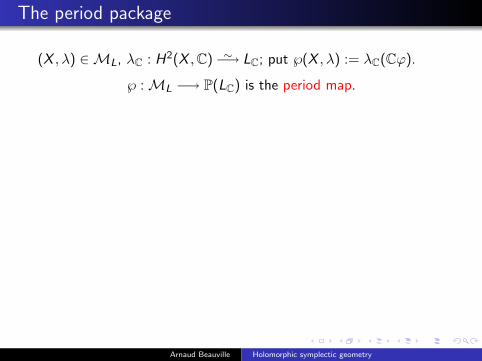
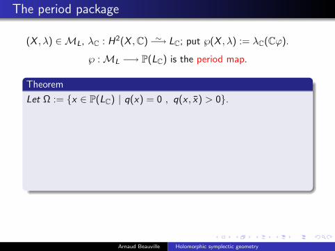
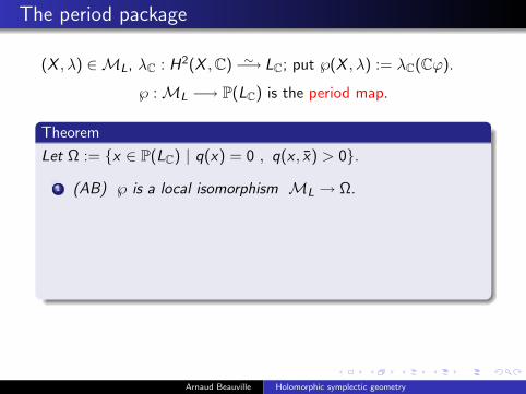
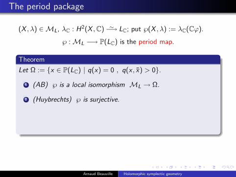
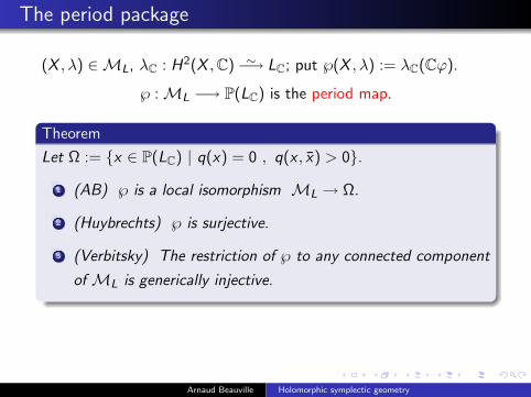
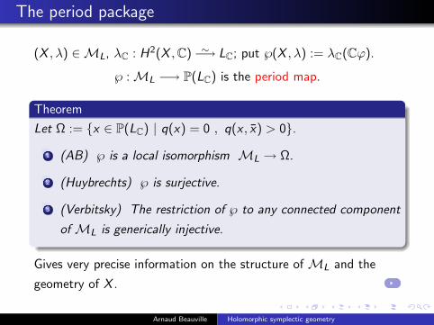
(X , λ) ∈ML, λC : H2(X ,C) ∼−→ LC; put ℘(X , λ) := λC(Cϕ).
℘ :ML −→ P(LC) is the period map.
Theorem
Let Ω := x ∈ P(LC) | q(x) = 0 , q(x , x) > 0.
1 (AB) ℘ is a local isomorphism ML → Ω.
2 (Huybrechts) ℘ is surjective.
3 (Verbitsky) The restriction of ℘ to any connected component
of ML is generically injective.
Gives very precise information on the structure of ML and the
geometry of X .
Arnaud Beauville Holomorphic symplectic geometry
The period package
(X , λ) ∈ML, λC : H2(X ,C) ∼−→ LC; put ℘(X , λ) := λC(Cϕ).
℘ :ML −→ P(LC) is the period map.
Theorem
Let Ω := x ∈ P(LC) | q(x) = 0 , q(x , x) > 0.
1 (AB) ℘ is a local isomorphism ML → Ω.
2 (Huybrechts) ℘ is surjective.
3 (Verbitsky) The restriction of ℘ to any connected component
of ML is generically injective.
Gives very precise information on the structure of ML and the
geometry of X .
Arnaud Beauville Holomorphic symplectic geometry
Completely integrable systems
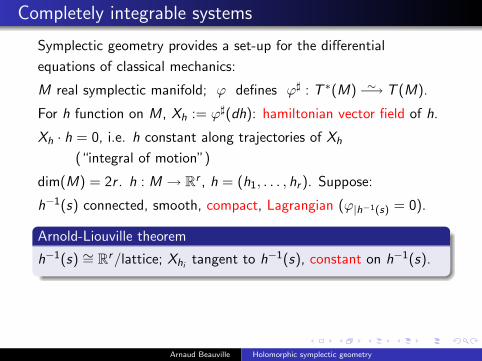
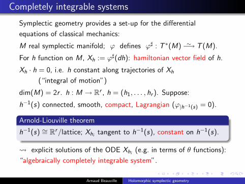
Symplectic geometry provides a set-up for the differential
equations of classical mechanics:
M real symplectic manifold; ϕ defines ϕ] : T ∗(M) ∼−→ T (M).
For h function on M, Xh := ϕ](dh): hamiltonian vector field of h.
Xh · h = 0, i.e. h constant along trajectories of Xh
(“integral of motion”)
dim(M) = 2r . h : M → Rr , h = (h1, . . . , hr ). Suppose:
h−1(s) connected, smooth, compact, Lagrangian (ϕ|h−1(s) = 0).
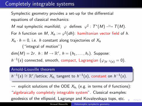
Arnold-Liouville theorem
h−1(s) ∼= Rr/lattice; Xhitangent to h−1(s), constant on h−1(s).
explicit solutions of the ODE Xhi(e.g. in terms of θ functions):
“algebraically completely integrable system”. Classical examples:
geodesics of the ellipsoid, Lagrange and Kovalevskaya tops, etc.
Arnaud Beauville Holomorphic symplectic geometry
Completely integrable systems
Symplectic geometry provides a set-up for the differential
equations of classical mechanics:
M real symplectic manifold; ϕ defines ϕ] : T ∗(M) ∼−→ T (M).
For h function on M, Xh := ϕ](dh): hamiltonian vector field of h.
Xh · h = 0, i.e. h constant along trajectories of Xh
(“integral of motion”)
dim(M) = 2r . h : M → Rr , h = (h1, . . . , hr ). Suppose:
h−1(s) connected, smooth, compact, Lagrangian (ϕ|h−1(s) = 0).
Arnold-Liouville theorem
h−1(s) ∼= Rr/lattice; Xhitangent to h−1(s), constant on h−1(s).
explicit solutions of the ODE Xhi(e.g. in terms of θ functions):
“algebraically completely integrable system”.
Classical examples:
geodesics of the ellipsoid, Lagrange and Kovalevskaya tops, etc.
Arnaud Beauville Holomorphic symplectic geometry
Completely integrable systems
Symplectic geometry provides a set-up for the differential
equations of classical mechanics:
M real symplectic manifold; ϕ defines ϕ] : T ∗(M) ∼−→ T (M).
For h function on M, Xh := ϕ](dh): hamiltonian vector field of h.
Xh · h = 0, i.e. h constant along trajectories of Xh
(“integral of motion”)
dim(M) = 2r . h : M → Rr , h = (h1, . . . , hr ). Suppose:
h−1(s) connected, smooth, compact, Lagrangian (ϕ|h−1(s) = 0).
Arnold-Liouville theorem
h−1(s) ∼= Rr/lattice; Xhitangent to h−1(s), constant on h−1(s).
explicit solutions of the ODE Xhi(e.g. in terms of θ functions):
“algebraically completely integrable system”. Classical examples:
geodesics of the ellipsoid, Lagrange and Kovalevskaya tops, etc.Arnaud Beauville Holomorphic symplectic geometry
Holomorphic set-up
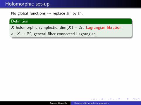
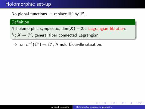
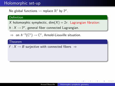
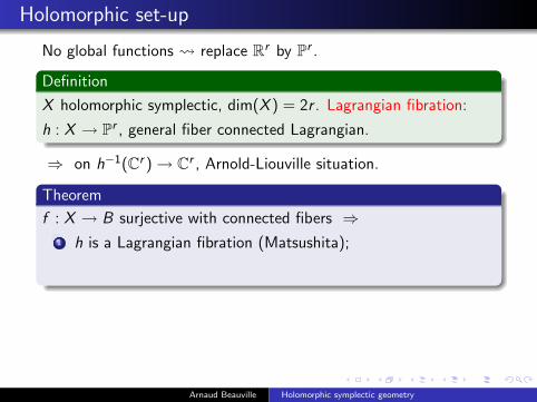
No global functions replace Rr by Pr .
Definition
X holomorphic symplectic, dim(X ) = 2r . Lagrangian fibration:
h : X → Pr , general fiber connected Lagrangian.
⇒ on h−1(Cr )→ Cr , Arnold-Liouville situation.
Theorem
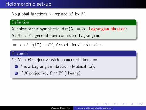
f : X → B surjective with connected fibers ⇒
1 h is a Lagrangian fibration (Matsushita);
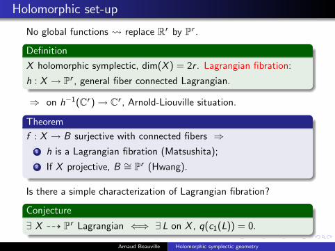
2 If X projective, B ∼= Pr (Hwang).
Is there a simple characterization of Lagrangian fibration?
Conjecture
∃ X 99K Pr Lagrangian ⇐⇒ ∃ L on X , q(c1(L)) = 0.
Arnaud Beauville Holomorphic symplectic geometry
Holomorphic set-up
No global functions replace Rr by Pr .
Definition
X holomorphic symplectic, dim(X ) = 2r . Lagrangian fibration:
h : X → Pr , general fiber connected Lagrangian.
⇒ on h−1(Cr )→ Cr , Arnold-Liouville situation.
Theorem
f : X → B surjective with connected fibers ⇒
1 h is a Lagrangian fibration (Matsushita);
2 If X projective, B ∼= Pr (Hwang).
Is there a simple characterization of Lagrangian fibration?
Conjecture
∃ X 99K Pr Lagrangian ⇐⇒ ∃ L on X , q(c1(L)) = 0.
Arnaud Beauville Holomorphic symplectic geometry
Holomorphic set-up
No global functions replace Rr by Pr .
Definition
X holomorphic symplectic, dim(X ) = 2r . Lagrangian fibration:
h : X → Pr , general fiber connected Lagrangian.
⇒ on h−1(Cr )→ Cr , Arnold-Liouville situation.
Theorem
f : X → B surjective with connected fibers ⇒1 h is a Lagrangian fibration (Matsushita);
2 If X projective, B ∼= Pr (Hwang).
Is there a simple characterization of Lagrangian fibration?
Conjecture
∃ X 99K Pr Lagrangian ⇐⇒ ∃ L on X , q(c1(L)) = 0.
Arnaud Beauville Holomorphic symplectic geometry
An example
Many examples of such systems. Here is one:
S ⊂ P5 given by P = Q = R = 0, P,Q,R quadratic ⇒ S K3.
Π = quadrics ⊃ S = λP + µQ + νR ∼= P2
Π∗ = dual projective plane = pencils of quadrics ⊃ S .
h : S [2] → Π∗ : h(x , y) = quadrics of Π ⊃ 〈x , y〉 .
By the theorem, h Lagrangian fibration ⇒
h−1(〈P,Q〉) = lines ⊂ P = Q = 0 ⊂ P5 ∼= 2-dim’l complex torus ,
a classical result of Kummer.
Arnaud Beauville Holomorphic symplectic geometry

II. Contact geometry
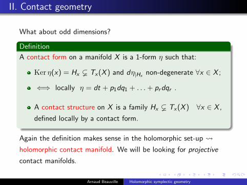
What about odd dimensions?
Definition
A contact form on a manifold X is a 1-form η such that:
Ker η(x) = Hx Tx(X ) and dη|Hxnon-degenerate ∀x ∈ X ;
⇐⇒ locally η = dt + p1dq1 + . . .+ prdqr .
A contact structure on X is a family Hx Tx(X ) ∀x ∈ X ,
defined locally by a contact form.
Again the definition makes sense in the holomorphic set-up
holomorphic contact manifold. We will be looking for projective
contact manifolds.
Arnaud Beauville Holomorphic symplectic geometry
II. Contact geometry
What about odd dimensions?
Definition
A contact form on a manifold X is a 1-form η such that:
Ker η(x) = Hx Tx(X ) and dη|Hxnon-degenerate ∀x ∈ X ;
⇐⇒ locally η = dt + p1dq1 + . . .+ prdqr .
A contact structure on X is a family Hx Tx(X ) ∀x ∈ X ,
defined locally by a contact form.
Again the definition makes sense in the holomorphic set-up
holomorphic contact manifold. We will be looking for projective
contact manifolds.
Arnaud Beauville Holomorphic symplectic geometry

Examples
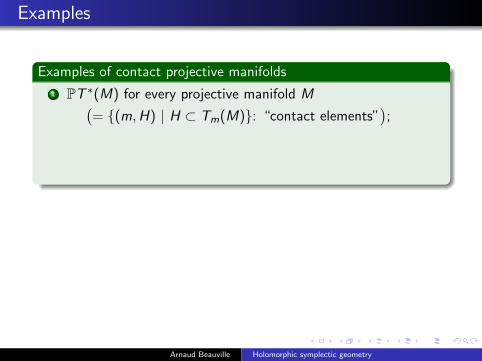
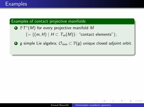
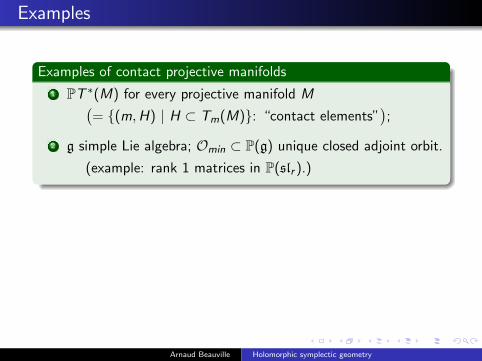
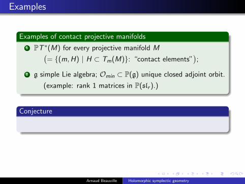
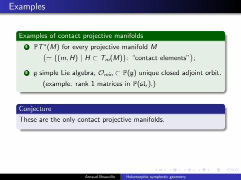
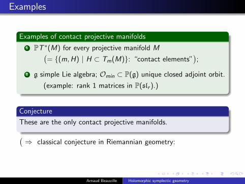
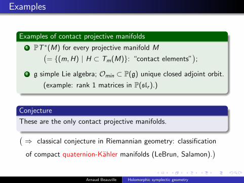
Examples of contact projective manifolds
1 PT ∗(M) for every projective manifold M(= (m,H) | H ⊂ Tm(M): “contact elements”
);
2 g simple Lie algebra; Omin ⊂ P(g) unique closed adjoint orbit.
(example: rank 1 matrices in P(slr ).)
Conjecture
These are the only contact projective manifolds.(⇒ classical conjecture in Riemannian geometry: classification
of compact quaternion-Kahler manifolds (LeBrun, Salamon).)
Arnaud Beauville Holomorphic symplectic geometry
Examples
Examples of contact projective manifolds
1 PT ∗(M) for every projective manifold M
(= (m,H) | H ⊂ Tm(M): “contact elements”
);
2 g simple Lie algebra; Omin ⊂ P(g) unique closed adjoint orbit.
(example: rank 1 matrices in P(slr ).)
Conjecture
These are the only contact projective manifolds.(⇒ classical conjecture in Riemannian geometry: classification
of compact quaternion-Kahler manifolds (LeBrun, Salamon).)
Arnaud Beauville Holomorphic symplectic geometry
Examples
Examples of contact projective manifolds
1 PT ∗(M) for every projective manifold M(= (m,H) | H ⊂ Tm(M): “contact elements”
);
2 g simple Lie algebra; Omin ⊂ P(g) unique closed adjoint orbit.
(example: rank 1 matrices in P(slr ).)
Conjecture
These are the only contact projective manifolds.(⇒ classical conjecture in Riemannian geometry: classification
of compact quaternion-Kahler manifolds (LeBrun, Salamon).)
Arnaud Beauville Holomorphic symplectic geometry
Examples
Examples of contact projective manifolds
1 PT ∗(M) for every projective manifold M(= (m,H) | H ⊂ Tm(M): “contact elements”
);
2 g simple Lie algebra; Omin ⊂ P(g) unique closed adjoint orbit.
(example: rank 1 matrices in P(slr ).)
Conjecture
These are the only contact projective manifolds.
(⇒ classical conjecture in Riemannian geometry: classification
of compact quaternion-Kahler manifolds (LeBrun, Salamon).)
Arnaud Beauville Holomorphic symplectic geometry
Examples
Examples of contact projective manifolds
1 PT ∗(M) for every projective manifold M(= (m,H) | H ⊂ Tm(M): “contact elements”
);
2 g simple Lie algebra; Omin ⊂ P(g) unique closed adjoint orbit.
(example: rank 1 matrices in P(slr ).)
Conjecture
These are the only contact projective manifolds.(⇒ classical conjecture in Riemannian geometry:
classification
of compact quaternion-Kahler manifolds (LeBrun, Salamon).)
Arnaud Beauville Holomorphic symplectic geometry
Examples
Examples of contact projective manifolds
1 PT ∗(M) for every projective manifold M(= (m,H) | H ⊂ Tm(M): “contact elements”
);
2 g simple Lie algebra; Omin ⊂ P(g) unique closed adjoint orbit.
(example: rank 1 matrices in P(slr ).)
Conjecture
These are the only contact projective manifolds.(⇒ classical conjecture in Riemannian geometry: classification
of compact quaternion-Kahler manifolds (LeBrun, Salamon).)
Arnaud Beauville Holomorphic symplectic geometry
Partial results
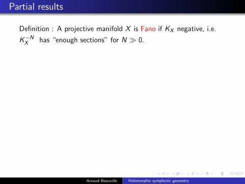
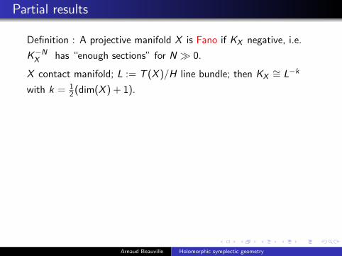
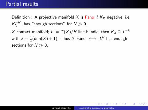
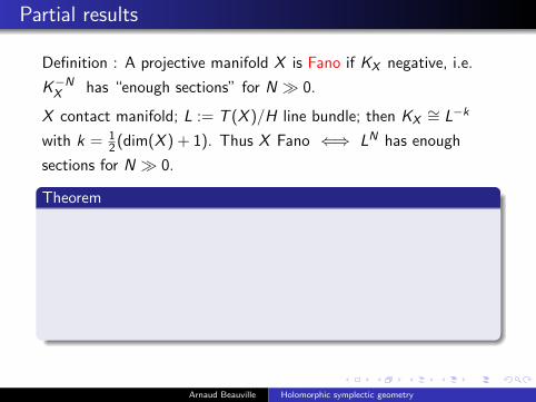
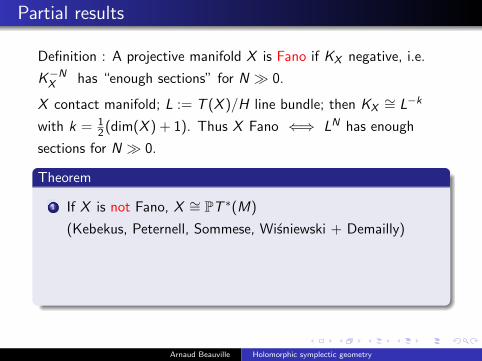
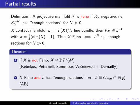
Definition : A projective manifold X is Fano if KX negative, i.e.
K−NX has “enough sections” for N 0.
X contact manifold; L := T (X )/H line bundle; then KX∼= L−k
with k = 12 (dim(X ) + 1). Thus X Fano ⇐⇒ LN has enough
sections for N 0.
Theorem
1 If X is not Fano, X ∼= PT ∗(M)
(Kebekus, Peternell, Sommese, Wisniewski + Demailly)
2 X Fano and L has “enough sections” ⇒ Z ∼= Omin ⊂ P(g)
(AB)
Arnaud Beauville Holomorphic symplectic geometry
Partial results
Definition : A projective manifold X is Fano if KX negative, i.e.
K−NX has “enough sections” for N 0.
X contact manifold; L := T (X )/H line bundle; then KX∼= L−k
with k = 12 (dim(X ) + 1).
Thus X Fano ⇐⇒ LN has enough
sections for N 0.
Theorem
1 If X is not Fano, X ∼= PT ∗(M)
(Kebekus, Peternell, Sommese, Wisniewski + Demailly)
2 X Fano and L has “enough sections” ⇒ Z ∼= Omin ⊂ P(g)
(AB)
Arnaud Beauville Holomorphic symplectic geometry
Partial results
Definition : A projective manifold X is Fano if KX negative, i.e.
K−NX has “enough sections” for N 0.
X contact manifold; L := T (X )/H line bundle; then KX∼= L−k
with k = 12 (dim(X ) + 1). Thus X Fano ⇐⇒ LN has enough
sections for N 0.
Theorem
1 If X is not Fano, X ∼= PT ∗(M)
(Kebekus, Peternell, Sommese, Wisniewski + Demailly)
2 X Fano and L has “enough sections” ⇒ Z ∼= Omin ⊂ P(g)
(AB)
Arnaud Beauville Holomorphic symplectic geometry
Partial results
Definition : A projective manifold X is Fano if KX negative, i.e.
K−NX has “enough sections” for N 0.
X contact manifold; L := T (X )/H line bundle; then KX∼= L−k
with k = 12 (dim(X ) + 1). Thus X Fano ⇐⇒ LN has enough
sections for N 0.
Theorem
1 If X is not Fano, X ∼= PT ∗(M)
(Kebekus, Peternell, Sommese, Wisniewski + Demailly)
2 X Fano and L has “enough sections” ⇒ Z ∼= Omin ⊂ P(g)
(AB)
Arnaud Beauville Holomorphic symplectic geometry
III. Poisson manifolds
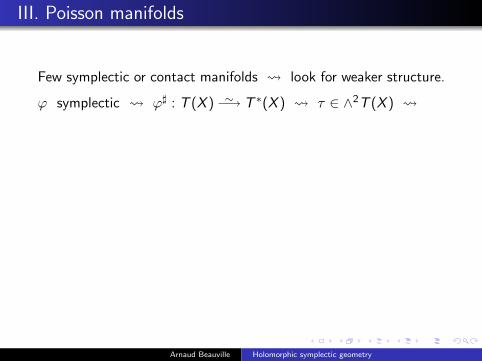
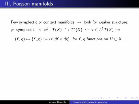
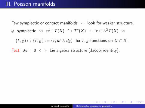
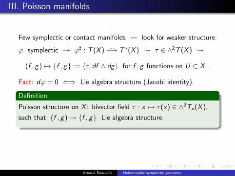
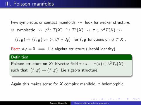
Few symplectic or contact manifolds look for weaker structure.
ϕ symplectic ϕ] : T (X ) ∼−→ T ∗(X ) τ ∈ ∧2T (X )
(f , g) 7→ f , g := 〈τ, df ∧ dg〉 for f , g functions on U ⊂ X .
Fact: dϕ = 0 ⇐⇒ Lie algebra structure (Jacobi identity).
Definition
Poisson structure on X : bivector field τ : x 7→ τ(x) ∈ ∧2Tx(X ),
such that (f , g) 7→ f , g Lie algebra structure.
Again this makes sense for X complex manifold, τ holomorphic.
Arnaud Beauville Holomorphic symplectic geometry
III. Poisson manifolds
Few symplectic or contact manifolds look for weaker structure.
ϕ symplectic ϕ] : T (X ) ∼−→ T ∗(X ) τ ∈ ∧2T (X )
(f , g) 7→ f , g := 〈τ, df ∧ dg〉 for f , g functions on U ⊂ X .
Fact: dϕ = 0 ⇐⇒ Lie algebra structure (Jacobi identity).
Definition
Poisson structure on X : bivector field τ : x 7→ τ(x) ∈ ∧2Tx(X ),
such that (f , g) 7→ f , g Lie algebra structure.
Again this makes sense for X complex manifold, τ holomorphic.
Arnaud Beauville Holomorphic symplectic geometry

Examples
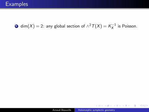
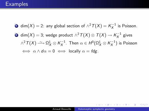
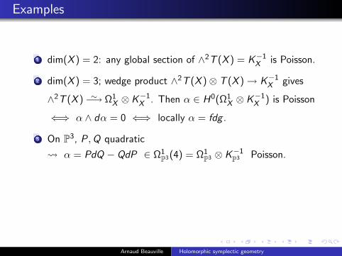
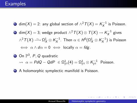
1 dim(X ) = 2: any global section of ∧2T (X ) = K−1X is Poisson.
2 dim(X ) = 3; wedge product ∧2T (X )⊗ T (X )→ K−1X gives
∧2T (X ) ∼−→ Ω1X ⊗ K−1
X . Then α ∈ H0(Ω1X ⊗ K−1
X ) is Poisson
⇐⇒ α ∧ dα = 0 ⇐⇒ locally α = fdg .
3 On P3, P,Q quadratic
α = PdQ − QdP ∈ Ω1P3(4) = Ω1
P3 ⊗ K−1P3 Poisson.
4 A holomorphic symplectic manifold is Poisson.
5 If X is Poisson, any X × Y is Poisson.
Arnaud Beauville Holomorphic symplectic geometry

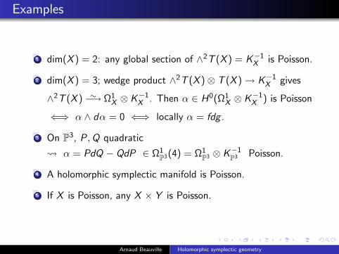
Examples
1 dim(X ) = 2: any global section of ∧2T (X ) = K−1X is Poisson.
2 dim(X ) = 3; wedge product ∧2T (X )⊗ T (X )→ K−1X gives
∧2T (X ) ∼−→ Ω1X ⊗ K−1
X . Then α ∈ H0(Ω1X ⊗ K−1
X ) is Poisson
⇐⇒ α ∧ dα = 0 ⇐⇒ locally α = fdg .
3 On P3, P,Q quadratic
α = PdQ − QdP ∈ Ω1P3(4) = Ω1
P3 ⊗ K−1P3 Poisson.
4 A holomorphic symplectic manifold is Poisson.
5 If X is Poisson, any X × Y is Poisson.
Arnaud Beauville Holomorphic symplectic geometry
The Bondal conjecture
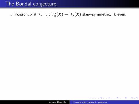
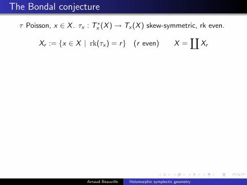
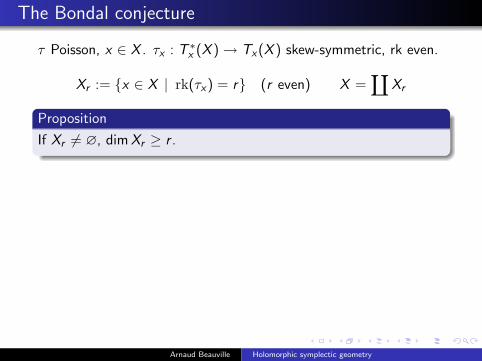
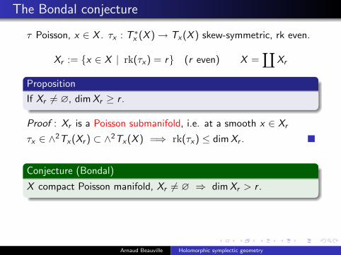
τ Poisson, x ∈ X . τx : T ∗x (X )→ Tx(X ) skew-symmetric, rk even.
Xr := x ∈ X | rk(τx) = r (r even) X =∐
Xr
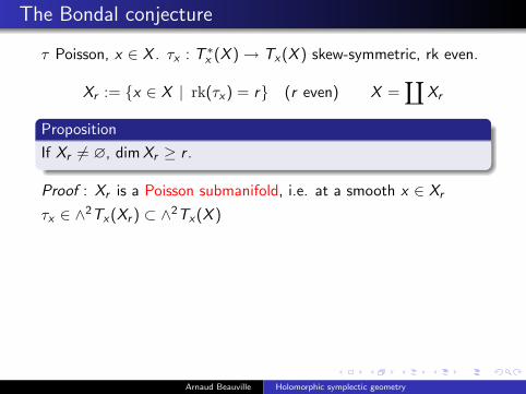
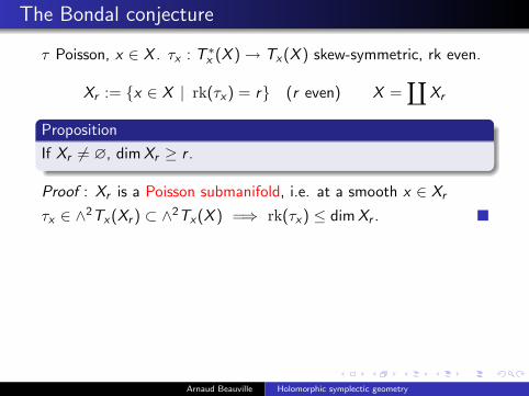
Proposition
If Xr 6= ∅, dim Xr ≥ r .
Proof : Xr is a Poisson submanifold, i.e. at a smooth x ∈ Xr
τx ∈ ∧2Tx(Xr ) ⊂ ∧2Tx(X ) =⇒ rk(τx) ≤ dim Xr .
Conjecture (Bondal)
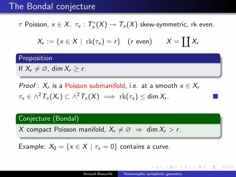
X compact Poisson manifold, Xr 6= ∅ ⇒ dim Xr > r .
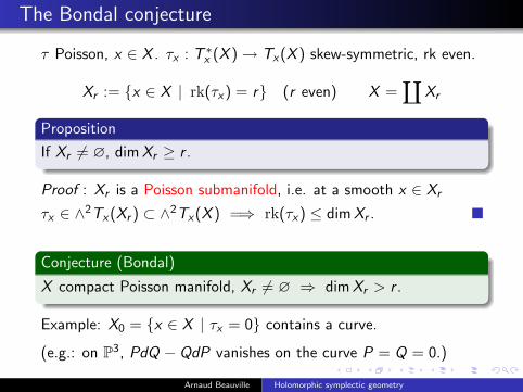
Example: X0 = x ∈ X | τx = 0 contains a curve.
(e.g.: on P3, PdQ − QdP vanishes on the curve P = Q = 0.)
Arnaud Beauville Holomorphic symplectic geometry
The Bondal conjecture
τ Poisson, x ∈ X . τx : T ∗x (X )→ Tx(X ) skew-symmetric, rk even.
Xr := x ∈ X | rk(τx) = r (r even) X =∐
Xr
Proposition
If Xr 6= ∅, dim Xr ≥ r .
Proof : Xr is a Poisson submanifold, i.e. at a smooth x ∈ Xr
τx ∈ ∧2Tx(Xr ) ⊂ ∧2Tx(X ) =⇒ rk(τx) ≤ dim Xr .
Conjecture (Bondal)
X compact Poisson manifold, Xr 6= ∅ ⇒ dim Xr > r .
Example: X0 = x ∈ X | τx = 0 contains a curve.
(e.g.: on P3, PdQ − QdP vanishes on the curve P = Q = 0.)
Arnaud Beauville Holomorphic symplectic geometry
The Bondal conjecture
τ Poisson, x ∈ X . τx : T ∗x (X )→ Tx(X ) skew-symmetric, rk even.
Xr := x ∈ X | rk(τx) = r (r even) X =∐
Xr
Proposition
If Xr 6= ∅, dim Xr ≥ r .
Proof : Xr is a Poisson submanifold, i.e. at a smooth x ∈ Xr
τx ∈ ∧2Tx(Xr ) ⊂ ∧2Tx(X )
=⇒ rk(τx) ≤ dim Xr .
Conjecture (Bondal)
X compact Poisson manifold, Xr 6= ∅ ⇒ dim Xr > r .
Example: X0 = x ∈ X | τx = 0 contains a curve.
(e.g.: on P3, PdQ − QdP vanishes on the curve P = Q = 0.)
Arnaud Beauville Holomorphic symplectic geometry
The Bondal conjecture
τ Poisson, x ∈ X . τx : T ∗x (X )→ Tx(X ) skew-symmetric, rk even.
Xr := x ∈ X | rk(τx) = r (r even) X =∐
Xr
Proposition
If Xr 6= ∅, dim Xr ≥ r .
Proof : Xr is a Poisson submanifold, i.e. at a smooth x ∈ Xr
τx ∈ ∧2Tx(Xr ) ⊂ ∧2Tx(X ) =⇒ rk(τx) ≤ dim Xr .
Conjecture (Bondal)
X compact Poisson manifold, Xr 6= ∅ ⇒ dim Xr > r .
Example: X0 = x ∈ X | τx = 0 contains a curve.
(e.g.: on P3, PdQ − QdP vanishes on the curve P = Q = 0.)
Arnaud Beauville Holomorphic symplectic geometry
The Bondal conjecture
τ Poisson, x ∈ X . τx : T ∗x (X )→ Tx(X ) skew-symmetric, rk even.
Xr := x ∈ X | rk(τx) = r (r even) X =∐
Xr
Proposition
If Xr 6= ∅, dim Xr ≥ r .
Proof : Xr is a Poisson submanifold, i.e. at a smooth x ∈ Xr
τx ∈ ∧2Tx(Xr ) ⊂ ∧2Tx(X ) =⇒ rk(τx) ≤ dim Xr .
Conjecture (Bondal)
X compact Poisson manifold, Xr 6= ∅ ⇒ dim Xr > r .
Example: X0 = x ∈ X | τx = 0 contains a curve.
(e.g.: on P3, PdQ − QdP vanishes on the curve P = Q = 0.)
Arnaud Beauville Holomorphic symplectic geometry
The Bondal conjecture 2
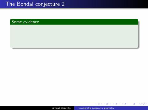
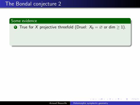
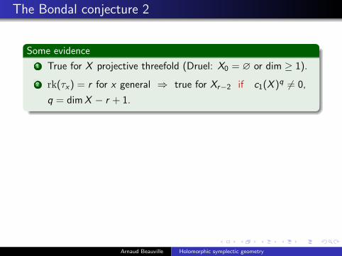
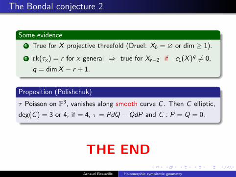
Some evidence
1 True for X projective threefold (Druel: X0 = ∅ or dim ≥ 1).
2 rk(τx) = r for x general ⇒ true for Xr−2 if c1(X )q 6= 0,
q = dim X − r + 1.
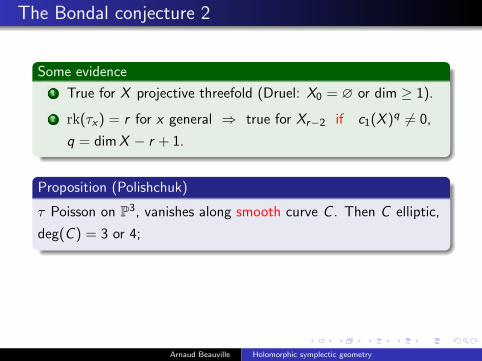
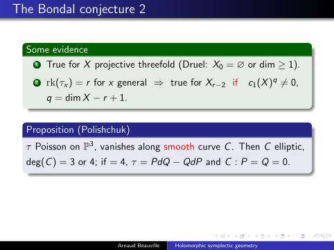
Proposition (Polishchuk)
τ Poisson on P3, vanishes along smooth curve C . Then C elliptic,
deg(C ) = 3 or 4; if = 4, τ = PdQ − QdP and C : P = Q = 0.
THE END
Arnaud Beauville Holomorphic symplectic geometry
The Bondal conjecture 2
Some evidence
1 True for X projective threefold (Druel: X0 = ∅ or dim ≥ 1).
2 rk(τx) = r for x general ⇒ true for Xr−2 if c1(X )q 6= 0,
q = dim X − r + 1.
Proposition (Polishchuk)
τ Poisson on P3, vanishes along smooth curve C . Then C elliptic,
deg(C ) = 3 or 4;
if = 4, τ = PdQ − QdP and C : P = Q = 0.
THE END
Arnaud Beauville Holomorphic symplectic geometry
The Bondal conjecture 2
Some evidence
1 True for X projective threefold (Druel: X0 = ∅ or dim ≥ 1).
2 rk(τx) = r for x general ⇒ true for Xr−2 if c1(X )q 6= 0,
q = dim X − r + 1.
Proposition (Polishchuk)
τ Poisson on P3, vanishes along smooth curve C . Then C elliptic,
deg(C ) = 3 or 4; if = 4, τ = PdQ − QdP and C : P = Q = 0.
THE END
Arnaud Beauville Holomorphic symplectic geometry
The Bondal conjecture 2
Some evidence
1 True for X projective threefold (Druel: X0 = ∅ or dim ≥ 1).
2 rk(τx) = r for x general ⇒ true for Xr−2 if c1(X )q 6= 0,
q = dim X − r + 1.
Proposition (Polishchuk)
τ Poisson on P3, vanishes along smooth curve C . Then C elliptic,
deg(C ) = 3 or 4; if = 4, τ = PdQ − QdP and C : P = Q = 0.
THE END
Arnaud Beauville Holomorphic symplectic geometry

![Nongeneric J-holomorphic curves and singular inflationopshtein/fichiers/nongen.pdfis regular in the usual sense for J-holomorphic curves; cf. [MS04, Chapter 3]. On the other hand,](https://static.fdocument.org/doc/165x107/60d7d746313b5e520851b38b/nongeneric-j-holomorphic-curves-and-singular-iniation-opshteinfichiersnongenpdf.jpg)
![arXiv:1506.08365v2 [math.CV] 4 Mar 2016 - …arXiv:1506.08365v2 [math.CV] 4 Mar 2016 TOPOLOGICAL INVARIANTS FOR SEMIGROUPS OF HOLOMORPHIC SELF-MAPS OF THE UNIT DISC FILIPPO BRACCI†,](https://static.fdocument.org/doc/165x107/5fdf8d2855bcae1548165a47/arxiv150608365v2-mathcv-4-mar-2016-arxiv150608365v2-mathcv-4-mar-2016.jpg)